Molecular Modelling - Lecture 2 Techniques for Conformational Sampling Uses CHARMM force field Written in C++

Molecular Modelling - Lecture 2 Techniques for Conformational Sampling Uses CHARMM force field Written in C++
Dec 13, 2015
Welcome message from author
This document is posted to help you gain knowledge. Please leave a comment to let me know what you think about it! Share it to your friends and learn new things together.
Transcript

Molecular Modelling - Lecture 2
Techniques for Conformational Sampling
Uses CHARMM force field
Written in C++

Protein example
QuickTime™ and aTIFF (LZW) decompressor
are needed to see this picture.
QuickTime™ and aTIFF (LZW) decompressor
are needed to see this picture.

Monte Carlo Simulations
Technique used to perform first computer simulation of a molecular system
“Monte Carlo” = some kind of random sampling

Monte Carlo Methods
Basis of Monte Carlo methods is the use of random selections in calculations that lead to the solution of numerical and physical problems e.g. brownian motion molecular modelling designing nuclear reactors predicting the evolution of stars forecasting the stock market
Each calculation is independent of the others and hence amenable to embarrassingly parallel methods

Monte Carlo Integration : finding value of πMonte Carlo integration
Compute r by generating random points in a square of side 2 and counting how many of them are in the circle with radius 1 (x2+y2<1; π=4*ratio) .
Area= π2
2
Area of square=4

Monte Carlo Simulations
Configurations are generated by making random changes to the positions of the atoms
Importance sampling Samples from 3N dimensional space of positions of
molecules

Monte Carlo Simulations
QuickTime™ and aTIFF (LZW) decompressor
are needed to see this picture.
QuickTime™ and aTIFF (LZW) decompressor
are needed to see this picture.
Z= Configurational integral

Metropolis Monte Carlo
Biases generation of configurations towards those that make the most significant contributions to the integral Low energy states for most thermodynamic
properties Generates states with probability
exp(xand counts them equally (simple Monte Carlo would generate them with equal
probability and then weight them by exp(x

QuickTime™ and aTIFF (LZW) decompressor
are needed to see this picture.
Markov chain of states

Monte Carlo Advantages/DisadvantagesAdvantages:
Does not require a continuous energy function (as in MD)
Number of particles can easily vary (very hard in MD)
Disadvantages Highly correlated motions hard to simulate
Poor sampling of large-scale changes

Molecular Dynamics
Newton’s equations of motions are integrated to propagate the structure through time
€
dx idt
= v i
dv idt
=Fim
Fi =∇ iE
Molecular Dynamics
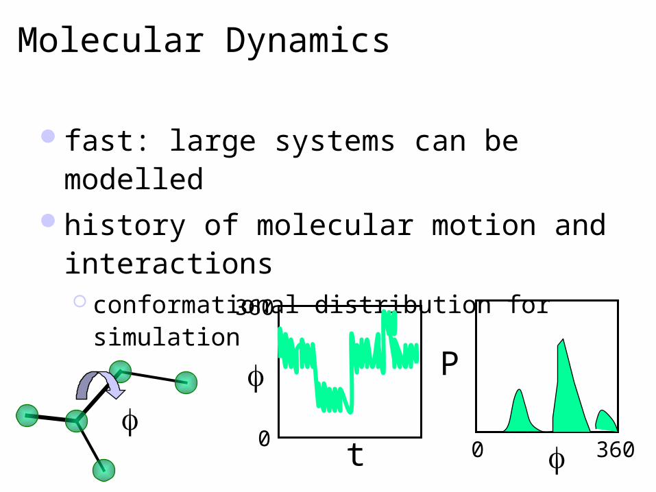
fast: large systems can be modelledhistory of molecular motion and
interactions conformational distribution for simulation
t
360
0
P
3600

Molecular Dynamics - Integration methodsFinite difference methods
Used to generate molecular dynamics trajectories with continuous potentials
Integration broken into stages separated by time t Total force on each particle at time t is calculated as a
vector sum of all the interactions with other particles From force can determine accelerations
Combined with positions and velocities at time t to calculate positions and velocities at time t + t
Force assumed to be constant during time step

Molecular Dynamics - Integration methodsMany algorithms:
Verlet Leap frog method Predictor-corrector Velocity-Verlet

Molecular Dynamics - Verlet Integration Method
QuickTime™ and aTIFF (LZW) decompressor
are needed to see this picture.
Most widely used method

Timescale Limitations
QuickTime™ and aTIFF (LZW) decompressor
are needed to see this picture.

MD Production Run Protocol
QuickTime™ and aTIFF (LZW) decompressor
are needed to see this picture.
Initial coords obtained from experimental data or theoretical model
Can be done by randomly selecting from a Maxwell-Boltzmann distribution at the temperature of interest

QuickTime™ and aTIFF (LZW) decompressor
are needed to see this picture.

QuickTime™ and aTIFF (LZW) decompressor
are needed to see this picture.

QuickTime™ and aTIFF (LZW) decompressor
are needed to see this picture.

Truncating Long-Range forces and the minimum image conventionNon-bonded interactions most time-
consuming part of a simulation N2
Minimum image convention: Interaction for a molecule i are only counted
between it and it’s closest image
Truncation of potential creates problems with consistent potential and force

Truncating Long-Range forces and the minimum image conventionUse smoothing functions to smoothly
switch off the interaction between a “cut-on” and a “cut-off” distance.
QuickTime™ and aTIFF (Uncompressed) decompressor
are needed to see this picture.

QuickTime™ and aTIFF (LZW) decompressor
are needed to see this picture.

Simulated Annealing
special case of either MD (`quenched' MD) or MC simulation, in which the temperature is gradually reduced during the simulation.
Often, the system is first heated and then cooled the system is given the opportunity to surmount
energetic barriers in a search for conformations with energies lower than the local-minimum energy found by energy minimization. can lead to more realistic simulations of dynamics at low
temperature more expensive than energy minimization.
Related Documents