NASA Contractor Report 4497 Planetary Biology and Microbial Ecology: Molecular Ecology and the Global Nitrogen Cycle Edited by Molly Stone Nealson and Kenneth H. Nealson Center for Great Lakes Studies Milwaukee, Wiscon.4n Prepared for NASA Office of Space 4cience and Applications under Grant NAGW-2136 National Aeronautics arid Space Administration Office of Management Scientific and Technic _1 Information Program 1993

Welcome message from author
This document is posted to help you gain knowledge. Please leave a comment to let me know what you think about it! Share it to your friends and learn new things together.
Transcript

NASA Contractor Report 4497
Planetary Biology and Microbial
Ecology: Molecular Ecology and
the Global Nitrogen Cycle
Edited by
Molly Stone Nealson and Kenneth H. Nealson
Center for Great Lakes Studies
Milwaukee, Wiscon.4n
Prepared for
NASA Office of Space 4cience and Applications
under Grant NAGW-2136
National Aeronautics aridSpace Administration
Office of Management
Scientific and Technic _1Information Program
1993


Table of Contents
Introduction vi
Schedule of Lectures arid Labs viii
Faculty, Lecturer and S:udent Addresses xviProtocols --
Molecular Techniques for the Identification and Study of
Luminous Bacteria
Quick Genomic DNA Isolation from Bacterial Colonies 2
Restriction Digest of Bacterial DNA 3Southern Blots 5
Prehybridization of Southern Blots 7
Hybridizati,_n of Southern Blots 8
Washing a-_d Exposing Southern Blcts 9
Colony Hybridization 13
The Polymerase Chain Reaction (PCR) 15
Cloning PCR Products into Single-st:anded Bacteriophage 16
Preparatior_ of M13 Sequencing Templates 23
DNA Sequ,._ncing 24
Classification of Bacteria Using 16S rRNA 33
cDNA Cloning Protocols
Extraction of Total RNA and Poly-(A)+-RNA 37
Construction of cDNA Library 43
Preparing High Specific Activity Sin!lie-Stranded 51cDNA Probes
Transfer ot Nucleic Acids to Nylon Membrane 53
and Conditions for Hybridization
DNA Sequencing with T7 DNA Polymerase (Sequenase) 56
Polymeras,_ Chain Reaction Assay Conditions 61
Preparatior= of Single-Stranded cDNA Synthesis for PCR 64
Cloning of DNA from PCR Amplification 64
Strategies lor Cloning and Characterizing cDNA 66
Appendix I" RACE 86
Appendix ;__:Screening a cDNA Clone by 89Immunochemical Methods
Appendix 3: Amplification of the Lambda Zap-II Library 91
Appendix 4: Extraction of High Molecular Weight DNA 92
Molecular Approaches to the Analysis of Population
Polymorphisms and Enzyme ExpressionRNA Isolation 94
Restriction Enzyme Digest 96In Vitro- Produced mRNA and cRNA 97
RNA Gel 98
Northern Blot 98
ooo
IIIPRE_EEH_tG P,_H3E BLANK NOT FILMED

Fragment Purification: Agarose 99
Random Priming 100mRNA to cDNA 101
Southern Blot 102
Hybridizations: RNA or DNA 103RNA Dot Blot 104
T4 DNA Polymerase 105
Media for Bacteria 106
Preservation of Animal Tissue at Room Temperature for 107
DNA AnalysesGeneclean: the Wonders of Glass and DNA 108
Boiling Minipreps for Plasmid DNA 109
iv

Lecturers' Abstracts and References
Edward DeLong Fluorescent Labeling of Amino-Oligonucleotides 111
Application of Molecular Genetic Techniques to 117
Microbial Ecology
Ann Giblin Overview of the Importance of Subtidal Sediments 122
to Nitrogen Cycling in Coastal Ecosystems]-he Importance of Benthic Macrofauna to Decom- 123
position and Nitrogen Cycting in Sediments
Heterocyst Differentiation and Nitrogen Fixation in 125
Cyanobacteria
Enzymes of Nitrification and Denitrification: Parts of 128
the Global NitrogenCycle
Use of Bulk Stable Isotopes for Environmental 133
Studies: Stable Isotopes at the Molecular Level
Energy Metabolism During Larval Development 138and Animal/Chemical Interactions in the Sea
Stable Isotopes and Their Use in Biogeochemical 139
Studies
Molecular Mechanisms Controlling Settlement and 141
Metamorphosis of Marine Invertebrate Larvae
Ecology of Luminous Bacteria 143Molecular Methods for the Identification and 146
Analysis of Phylogenedc Relationships Among
Subsurface Microorganisms
Gene Expression in Symbiotically Associated and 147
Free-Living Cyanobacteria
David L. Peterson Remote Sensing of Ecosystems and Simulation of 148
Ecosystem Processes
Thomas Schmidt Molecular Phylogenies and Microbial Evolution 159
Identification and Quantilication of Microorganisms 160
in Natural Habitats Using rRNA-Based Probes
Simon Silver Transport Across the Cell Surface: Good 163
Substrates and Bad
Biochemistry and Molecular Biology of Bacterial 164
Resistances to Toxic Heavy Metals
Metallothioneins: Small Cadmium-Binding Proteins 165
from Horses, Plants and Bacteria
Mitchell L. Sogin Recent Developments in Phylogeny of Eukaryotes 1 67
Ivan Valiela An Overview of Nitrogen Cycling in Marine and 169
Aquatic SystemsAbbreviations 170
Robert Haselkorn
Thomas Hollocher
Stephen Macko
Donal Manahan
Joseph Montoya
Daniel E. Morse
Kenneth H. Nealson
Sandra Nierzwicki-
Bauer
Appendix:
V

Introduction
In the summer of 1991, the NASA Planetary Biology and Molecular
Ecology (PBME) program was conducted at the Marine Biological Laboratory
(MBL) in Woods Hole, Massachusetts. The program used the facilities of
the MBL, including the laboratories, dormitories, cafeteria, and laboratory
support system. This was the fifth course in a series of PBME programs,
and was only the second to be conducted at a site remote from the NASAAmes Research Center.
The goals of this intensive summer program were twofold: (1) to
examine, via lectures and discussions, several aspects of the
biogeochemistry of the nitrogen cycle; and (2) to teach the application of
modern methods of molecular genetics to field studies. In this sense, this
year's program differed from some of the previous PBME courses, which
centered more on microbiology. Here we focused on teaching modern
approaches to environmental studies of organisms, including not only
microbes, but also phylogenetically more advanced forms.
To accomplish the first goal, a distinguished group of scientists was
invited to lecture on various aspects of biogeochemistry, specifically the
biogeochemistry of nitrogen. The lectures covered many areas, including
the biogeochemical cycling of nitrogen in freshwater, estuarine, marine, and
terrestrial ecosystems. The lecturers included ecologists, physiologists,
biochemists, molecular biologists, and ecosystems scientists. Abstracts ofand references for the individual talks are presented in this document.
Of particular note for the goals of the course was the series of
lectures given by Dr. David Peterson of the NASA Ames Research Center.
These lectures, in combination with those involving stable isotope
geochemistry and general biogeochemistry, form a basis for analysis of the
nitrogen cycle, and how to relate many of the methods taught here to more
broadly based problems.
To accomplish the second goal, both lectures and laboratory
exercises were utilized. Three laboratory modules were run consecutively,
each an intensive training session of two weeks. These modules were
originated and supervised by Dr. Charles Wimpee, Dr. Thomas Chen, and
Dr. Dennis Powers, and dealt with molecular biology of bacteria, fish, and
mitochondria, respectively. A list of those faculty members and their
teaching assistants, directly involved in the laboratory teaching, is included
below. Laboratory education consisted of extensive lecture periods
discussing both techniques and approaches, coupled with "hands-on"
laboratory exercises.
vi

Wimpee Module: Mol_cular Biology of Bioluminescent Bacteria
Dr. Charles Wimpee, Univ. of Wisconsin-Milwaukee
Assisted by Dr. Daad Saffarini
Assisted by Denise Garvin
Chen Module: cDNA Cloning
Dr. Thomas Chen, Center of Marine Biotechnology, Univ. Maryland
Assisted by Dr. Chun-Mean Lin
Assisted by Michael Shamblott
Assisted by Bih-Ying Yang
Powers Module: Population Polymorphisms and Enzyme Expression
Dr. Douglas Crawford, Univ. of Chicago
Dr. Simona Ba_tl, Hopkins Marine Station, Stanford Univ.
Assisted by Stephanie Clendennen
Detailed descriptions of the laboratory projects and protocols for each
of the three modules are contained in this report. Through this
presentation, we have attempted to bring the material to others who mightfind it valuable.
Previous NASA PBME courses have used somewhat different
approaches. They a(e described in NASA Technical Memorandum #86043
(Carbon Cycling), NASA Technical Memorandum #87570 (Sulfur Cycling),
and NASA Contractor Report #4295 (Metal Cycling). Because of the
different goals of the laboratory work in this course, the format was quite
different than used in previous years. As with the previous courses,
however, the experience proved to be exceptionally valuable for the transfer
of information and techniques between ecologists, geochemists, and NASA
personnel.
vii
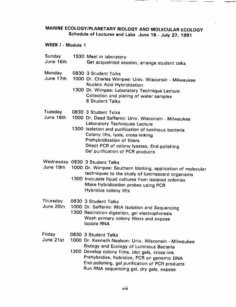
MARINE ECOLOGY/PLANETARY BIOLOGY AND MOLECULAR ECOLOGY
Schedule of Lectures and Labs June 16 - July 27, 1991
WEEK I - Module 1
SundayJune 16th
1930 Meet in laboratory
Get acquainted session, arrange student talks
Monday 0830June 17th 1000
1300
3 Student Talks
Dr. Charles Wimpee: Univ. Wisconsin - Milwaukee
Nucleic Acid Hybridization
Dr. Wimpee: Laboratory Technique Lecture
Collection and plating of water samples6 Student Talks
Tuesday 0830June 18th 1000
1300
3 Student Talks
Dr. Daad Saffarini: Univ. Wisconsin - Milwaukee
Laboratory Techniques Lecture
Isolation and purification of luminous bacteria
Colony lifts, lysis, cross-linking
Prehybridization of filters
Direct PCR of colony lysates, End-polishing
Gel purification of PCR products
Wednesday 0830June 19th 1000
1300
3 Student Talks
Dr. Wimpee: Southern blotting, application of molecular
techniques to the study of luminescent organisms
Inoculate liquid cultures from isolated colonies
Make hybridization probes using PCR
Hybridize colony lifts
Thursday 0830June 20th 1000
1300
3 Student Talks
Dr. Saffarini: RNA Isolation and Sequencing
Restriction digestion, gel electrophoresis
Wash primary colony filters and exposeIsolate RNA
Friday 0830June 21st 1000
1300
3 Student Talks
Dr. Kenneth Nealson: Univ. Wisconsin - Milwaukee
Biology and Ecology of Luminous Bacteria
Develop colony films, blot gels, cross-link
Prehybridize, hybridize, PCR on genomic DNA
End-polishing, gel purification of PCR products
Run RNA sequencing gel, dry gels, expose
viii
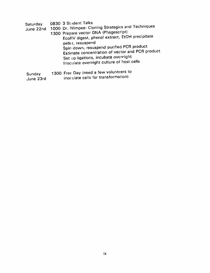
SaturdayJune 22nd
083010001300
3 St_._dentTalksDr. Wimpee: Cloning Strategi_.,sand TechniquesPrepare vector DNA (Phagescript)EcoRV digest, phenol extract, EtOH precipitatepell_t, resuspendSpin down, resuspend purified PCR productEstimate concentration of vector and PCR productSet up ligations, incubate overnightInoculate overnight culture o! host cells
SundayJune 23rd
1300 FreE.Day (need a few voluntE;erstoinoculate cells for transformation)
ix
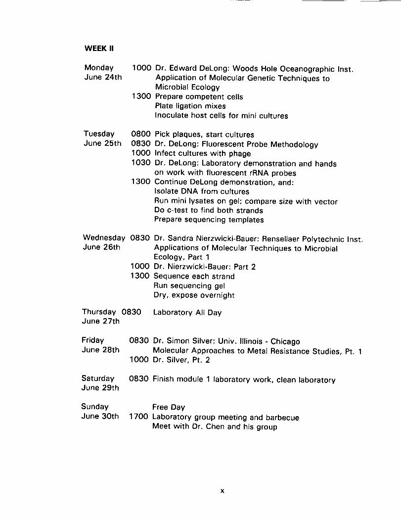
WEEK II
Monday 1000June 24th
1300
Dr. Edward DeLong: Woods Hole Oceanographic Inst.
Application of Molecular Genetic Techniques to
Microbial Ecology
Prepare competent cells
Plate ligation mixes
Inoculate host cells for mini cultures
Tuesday 0800June 25th 0830
1000
1030
1300
Pick plaques, start cultures
Dr. DeLong: Fluorescent Probe Methodology
Infect cultures with phage
Dr. DeLong: Laboratory demonstration and hands
on work with fluorescent rRNA probes
Continue DeLong demonstration, and:Isolate DNA from cultures
Run mini lysates on gel; compare size with vectorDo c-test to find both strands
Prepare sequencing templates
Wednesday 0830June 26th
1000
1300
Dr. Sandra Nierzwicki-Bauer: Rensellaer Polytechnic Inst.
Applications of Molecular Techniques to Microbial
Ecology, Part 1Dr. Nierzwicki-Bauer: Part 2
Sequence each strand
Run sequencing gel
Dry, expose overnight
Thursday 0830June 27th
Laboratory All Day
FridayJune 28th
0830 Dr. Simon Silver: Univ. Illinois - Chicago
Molecular Approaches to Metal Resistance Studies, Pt. 11000 Dr. Silver, Pt. 2
SaturdayJune 29th
0830 Finish module 1 laboratory work, clean laboratory
SundayJune 30th
Free Day
1700 Laboratory group meeting and barbecue
Meet with Dr. Chen and his group
X

WEEK III - Module 2
Monday 0830
July 1st1000
Dr. David Peterson: NASA Arnes Research Center
Remote Sensing of Forest EcosystemsIsolation of total RNA
Tuesday 0830
July 2nd 1000
Dr. Peterson: Remote Sensin!] and the Nitrogen Cycle
Isol_]tion of poly(A)+-RNA arid agarose gel
electrophoresis
Wednesday 0830
July 3rd
1000
1300
2000
Dr. Thomas Chen: Center of Marine Biotechnology,
University of Maryland
I. Structure, Evolution and R_._gulation of Fish GrowthHormone Genes
II. "_ransgenic Fish Approaches to Marine Systems
SyrTthesis of 1st and 2nd strand cDNA, RACE synthesis
of _;DNA and precipitation o! cDNA
Dr. Wimpee: Non-photosynthetic Parasitic Plants
Thursday 0830
July 4th 1000
1800
Laboratory Lecture - Dr. Chen
Ca!culation of cDNA synthe.';ized, methylation, linker I
ligation and isolation of genomic DNA from red cellsVolleyball, fireworks at Nob:{ka Point
Friday
July 5th
0830
1000
1300
Dr Thomas Schmidt: Miami University, Ohio
I. Molecular Phylogenies and Microbial Evolution
I1. Identification Without Cultivation: Using rRNA's to
StJdy Marine Picoplankton
Tr mming of excess linkers, precipitation of cDNA
Ligation of cDNA to lada Zap vector
Saturday
July 6th
0830 In vitro packagingTi_er estimation
Sunday
July 7th
Free Day (plating out for screening)
xi
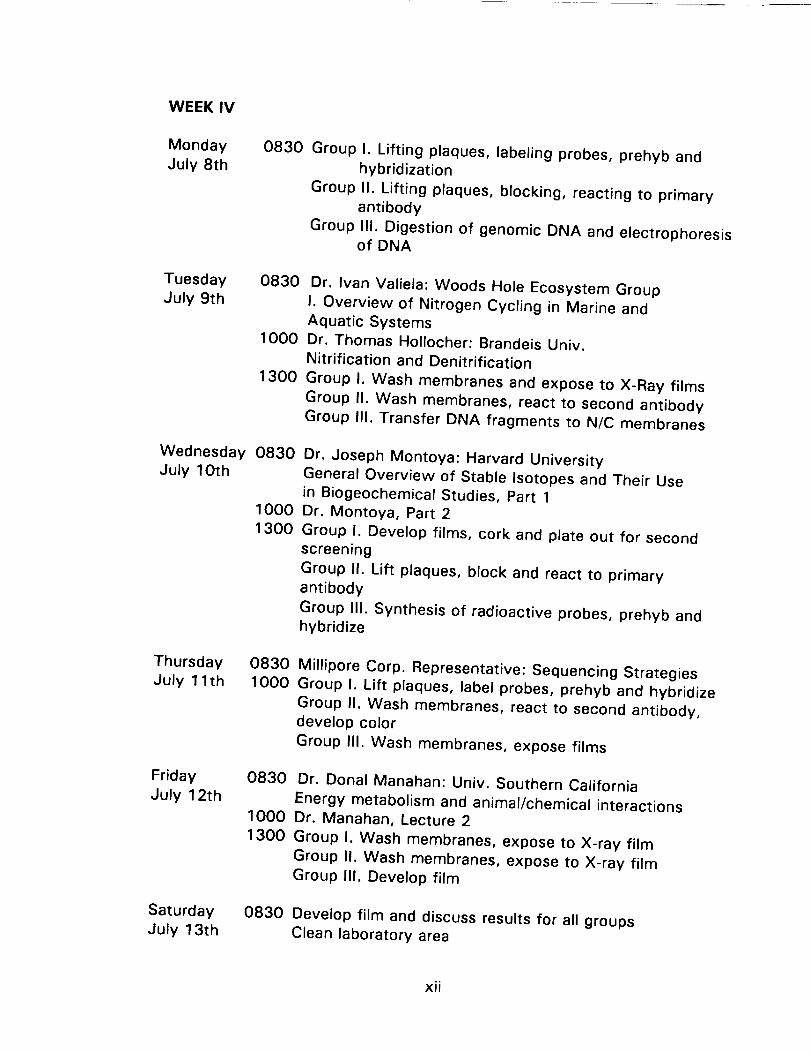
WEEK IV
Monday
July 8th
0830 Group I. Lifting plaques, labeling probes, prehyb and
hybridization
Group I1. Lifting plaques, blocking, reacting to primary
antibody
Group III. Digestion of genomic DNA and electrophoresisof DNA
Tuesday 0830
July 9th
1000
1300
Dr. Ivan Valiela: Woods Hole Ecosystem Group
I. Overview of Nitrogen Cycling in Marine and
Aquatic SystemsDr. Thomas Hollocher: Brandeis Univ.
Nitrification and Denitrification
Group I. Wash membranes and expose to X-Ray films
Group I1. Wash membranes, react to second antibody
Group III. Transfer DNA fragments to N/C membranes
Wednesday 0830
July lOth
1000
1300
Dr. Joseph Montoya: Harvard University
General Overview of Stable Isotopes and Their Use
in Biogeochemical Studies, Part 1
Dr. Montoya, Part 2
Group I. Develop films, cork and plate out for second
screening
Group I1. Lift plaques, block and react to primary
antibody
Group II1. Synthesis of radioactive probes, prehyb and
hybridize
Thursday 0830
July 1 lth 1000
Millipore Corp. Representative: Sequencing Strategies
Group I. Lift plaques, label probes, prehyb and hybridize
Group II. Wash membranes, react to second antibody,
develop color
Group II1. Wash membranes, expose films
Friday 0830
July 12th1000
1300
Dr. Donal Manahan: Univ. Southern California
Energy metabolism and animal/chemical interactions
Dr. Manahan, Lecture 2
Group I. Wash membranes, expose to X-ray film
Group II. Wash membranes, expose to X-ray film
Group III. Develop film
Saturday
July 13th
0830 Develop film and discuss results for all groups
Clean laboratory area
xii

WEEK V - Module 3
Monday 0830
July 15th
1000
1300
Dr. De_lnis Powers: Hopkins Marine Stn, Stanford Univ.
Overview of Genetic and Biochemical Approaches to
the Study of Marine systems, Part 1Dr. Powers: Part 2
Laboratory Lecture: population markers, PCR primers
Get animals, begin genomic DNA prep
Discuss designing primers, finish DNA prep
Tuesday 0830
July 16th
Determine DNA yields and analyze on gel
Go over primer design, examine gels
Set up PCR experiments, digest cloning vehicles
Prepare next round of PCR samplesStart second round of PCRs
Wednesday 0700
July 17th 08000900
Load gels with PCR samples and digested vectorsBreaklast
Examiqe gels, clean up PCR products
Digesl PCR products for cloning
Clean up digested vectors, run on low-melt agarose
Purify fragments from gel
Precipitate PCR products and vector together
Set up ligations
Transform competent bacteria, plate bacteria
Thursday 0830
July 18th1300
Dr. Daniel Morse: Univ. California - Santa Barbara
Ecology and Biology of Larval Settlement
Clean up additional PCR products
Digest: PCR products for population polymorphism study
Start oacterial cultures for ssDNA prep.
Gel ar_alyze PCR product polymorphisms
Pour .';equencing gels for tomorrow
Friday 0830
July 19th
1300
Dr. Stephen Macko: Univ. Virginia
Use of Bulk Stable Isotopes for Environmental Studies
Stable Isotopes at the Molecular Level
ssDNA preps, sequencing reactions, sequencing gels
Seco_d loading, soak and dry !]el, put down for autorad
Saturday
July 20th
0830 Read sequencing gels and analyze data
Finish any loose ends, discuss data, clean lab areas
Sunday
July 21 st
Free Day
xiii

WEEK VI
Monday 0830
July 22nd
1000
1300
Tuesday 0830
July 23rd
Wednesday 0700
July 24th 0830
1300
Thursday 0830
July 25th
Dr. Ann Giblin: Woods Hole Ecosystem Center
Nitrogen Cycling in Atlantic Coastal Ecosystems
Involvement of Eucaryotic Organisms in the N-Cycle
mRNA isolation, prep for centrifugation
Sp6 plasmid digest, pour gel for RNA analysis
Finish RNA prep from centrifuge
Determine yield, gel analyses
Set up Northern, medium, digest p440
Electrophoresis of p440, low melt
Gel purification of p440
Synthesize cRNA from Sp6 vector
Determine cRNA yieldsDot blots
Prehyb. dot blot and northern of LDH probe
Mitochondrial DNA prep
Digest mitochondrial DNA
Dr. Robert Haselkorn: Univ. Chicago
Regulation of Heterocyst Differentiation in Cyanobacteria
Molecular Biology of Cyanobacteria
Gel electrophoresis of mitochondrial DNA
Random prime p440 fragment (2X)
Add label fragment to dot blot, northern
Pressure blot mtc DNA, prehybridize mtc blot
Random prime mtc DNAAdd labeled mtc DNA to Southern
RNA to cDNA
PCR LDH-B cDNA
Digest with restriction enzymes
Acrylamide gel electrophoresis of cDNAElectroblot
Prehybridize LDH-B cDNA blot
Wash dot blot and mtc DNA blot
Put filters onto film
Add labeled p440 to cDNA blot
xiv
FridayJuly 26th
SaturdayJuly 27th
0830 Dr. Mitchell Sogin: Marine Biological Labs
Recent Developments in the Phylogeny of Eucaryotes
1300 Cut up dot blot, count activityWash [DH-B cDNA blot
Put on film
Develoo mtc and cDNA blots
Analyze.' data
0830 Review results
Clean up loose ends, clean up lab areas
XM

FACULTY, LECTURER, AND STUDENT ADDRESSES
University/Institution Home/Permanent
Barnhisel, Rae
Dept. of Biological Sciences
Michigan Technological Univ.
Houghton, MI 49931
(906) 487-2275 (2025 message)
311 Harris Ave.
Hancock, MI
49930
(906) 482-0744
Bartl, Simona
Hopkins Marine Station
Pacific Grove, CA 93950-3094
(408) 655-6218 (408) 655-2908
Bennison, Brenda
Dept. of Biological SciencesFlorida State Univ.
Tallahassee, FL 32306
(904) 644-0720
1318 Circle Dr.
Tallahassee, FL
32301
(904) 878-3547
Bernhard, JoanWadsworth Center for Labs & Rsrch
New York State Dept. of Health
PO Box 509, Empire State Plaza
Albany, NY 12201-0509
(518) 473-3779 or 3856
4870 Schurr Rd.
Clarence, NY
14031
(716) 759-6733
Blakemore, Richard
Dept. of Microbiology
Univ. of New Hampshire
Durham, NH 03824
(603) 862-2211
4 Davis Ave.
Durham, NH
03824
Booth, Cheryl
Univ. of Wisconsin
624 Langdon #104
Madison, WI 53703
65 Grasmere Dr.
Falmouth, MA
02540
Buchholz, LorieCenter for Great Lakes Studies
600 E. Greenfield Ave.
Milwaukee, Wl 53204
(414) 382-1727
xvi

Calderon, FranciscoDept. of Crop & Soil Sci.
Michigan State Univ.
East Lansing, MI 48824-1325
0-53 Ave. Park Gardens
Rio Piedras, Puerto Rico00926
(809) 761-7917
Campbell, Douglas
Physiologie Microbienne
Dept. B.G.M., Institut Pasteur
28, rue du Dr.Roux75724 Paris
CEDEX 15
Chen, Thomas
Center of Marine Biote_:hnology
Univ. of Maryland600 E. Lombard St.
Baltimore, MD 21202
(301) 783-4830 or 4806
Clendennen, Stephanie
Hopkins Marine Statior}
Pacific Grove, CA 93950-3094
(408) 373-0464
Collins, Amy L. Tsui
Finnegan, Henderson, Farabow, Garrett & Dunner
1300 I Street, N.W.
Washington, DC 20005-3315
(202) 408-4000
Crawford, Douglas
Dept. Organismal Bio & Anatomy
Univ. of Chicago1025 E. 57th St.
Chicago, IL 60637(312) 702-8097
DeLong, Edward
Dept. of BiologyUniv. of California - Santa Barbara
Santa Barbara, CA 93106
(805) 893-7245
xvii

Dutcher, Julie
Center for Marine Science Research
7205 Wrightsville Ave.
Wilmington, NC 28403
(919) 256-3721 or 350-4038
Garvin, Denise
PO Box 413, Biology Dept.Univ. WI-Milwaukee
Milwaukee, WI 53201
(414) 229-6881
Giblin, Ann
Woods Hole Ecosystem Center
Woods Hole, MA 02543
(508) 548-3705 ext. 488
Haselkorn, Robert
Dept. of Cellular & Molecular Biology
University of Chicago
Chicago, IL 60637(312) 702-1069
Henderson, Phyllis
Science Dept.
Truckee Meadows Community College7000 Dandir_i Blvd.
Reno, NV 89502
(702) 673-7023
Holland, Brenden
Dept. of OceanographyTexas A&M Univ.
College Station, TX 77843(409) 845-6896 or 8217
Hollocher, Thomas
Dept. of BiochemistryBrandeis Univ.
Waltham, MA
(617) 736-2345
PO Box 146
Wrightsville Beach, NC28480
(919) 256-6434
1695 Auburn Way
Reno, NV89502
(702) 329-3776
28 Roble Rd.
Berkeley, CA94705
(415) 841-0556
xviii

Juinio, Annette R.Marine Science Inst.UPPO Box 1Univ. of the PhilippinesDiliman, Quezon City 1101Philippines
Kemp, Paul F.Ocean. & Atmos. Sci. Division
Brookhaven National Labc_ratory
Upton, NY 11973
(516) 282-7697
(516) 282-2060
Ladner, Bob
U. of Medicine & DentistTy of NJ
School of Osteopathic Mt,_dicine401 South Central Plaza
Stratford, NJ 08084
(609) 782-6043
Lin, Chun-Mean
COMB, U. of MD600 E. Lombard St.
Baltimore, MD 21202
(301) 783-4831
Macko, Steven
Dept. Environmental Sci{,nces
Univ. of Virginia
Charlottesville, VA 22903
(804) 982-2967
Manahan, Donal
Univ. of Southern California
Dept. of Biological Sciences
Los Angeles, CA 90089-0371
(213) 740-5793
Miller, Daniel
Cornell University
Microbiology, 112 Wing Hall
Ithaca, NY 14850
(607) 255-3088
25 P. Burgos St.
Pasig, Metro Manila
Philippines
(63) 2-682-2515
86 Cedar St.
Stony Brook, NY11790
(516) 689-2829
703 Greenman Rd.
Haddonfield, NJ
08033
(609) 428-3376
804 Cayuga Hgts. Rd.
Ithaca, NY 14850
xix

Miller, Kathy Ann
Biology Dept.
Univ. of Puget SoundTacoma, WA 98416
(206) 756-3132
704 N. Cushman
Tacoma, WA98403
(206) 627-724
Montoya, Joseph
Harvard University
179 Biological Labs
16 Divinity Ave.
Cambridge, MA 02138(617) 496-8537
Morse, AileenMarine Science Institute
UC Santa Barbara
Santa Barbara, CA 93106
(805) 893-3416
Morse, Daniel
Marine Science Institute
UC Santa Barbara
Santa Barbara, CA 93106
(805) 893-3416
Nealson, Ken
Center for Great Lakes Studies
600 E. Greenfield Ave.
Milwaukee, Wl 53204
(414) 382-1706
4448 S. Lawler Ave.
Cudahy, Wl53111
(414) 769-8030
Nierzwicki-Bauer, Sandra
Dept. of Biology
Rensellaer Polytechnical Institute
Troy, NY 12181(518) 276-2699
Peterson, David
NASA Ames Res. Center, Mail-Stop 242-4
Moffett Field, CA 94022
(415) 604-5899
XX
Powers, Dennis
Hopkins Marine Station, Stanford Univ.
Pacific Grove, CA 93950
(408) 373-0674
Rawson, Paul
Dept. Biological SciencesUniv. of South Carolina
Columbia, SC 29208
(803) 777-6629
Rohatgi, Raj
Harvard College
Cambridge, MA 021:38
Saffarini, DaadCenter for Great Lakes Studies
600 E. Greenfield Ave.
Milwaukee, Wl 53204
(414) 382-1712
Sanger, Joseph
Dept. of Anatomy
U. Penn, School of Medicine36th & Hamilton Walk
Philadelphia, Pa 19104-6085
(215) 898-6919
Schulte, Trish
Hopkins Marine Station
Pacific Grove, CA 93950
(408) 373-0464
Schmidt, Thomas
Dept. of Biology
Miami University
Oxford, OH 45056
(513) 529-1694
Schwartz, David
Calhoun College Dean's Office245-A Yale Station
New Haven, CT 06520
(203) 432-0744
2812 Grace St.
Columbia, SC29201
(803) 779-8732
4759 N. Marlborough Dr.
Whitefish Bay, Wl 53211
601 Parrish Rd
Swarthmore, PA19081
(203) 432-0737
xxi

Shamblott, MikeCOMB 600 E. Lombard St.
Baltimore, MD 21202
(301) 783-4831
Silver, Simon
Dept. Microbiology & Immunology (M/C 790)
Univ. Illinois-Chicago, College of Medicine
Chicago, IL 60680
(312) 996-9608
Sogin, Mitchell
Marine Biological Laboratory
Woods Hole, MA 02543
(508) 548-3705
Swanson, Willie
c/o Vacquier Lab
Scripps Inst. OceanographyUCSD 9500 Gilman Dr.
La Jolla, Ca 92093-0202
(619) 534-2146
3 Harvey Ct.
Irvine, CA92715
(714) 725-0643
Toolan, Tara
MCZ Labs 504, Harvard Univ.
26 Oxford St.
Cambridge, MA 02138
(617) 495-5627
(617) 495-0506 FAX
Tosques, Ivan
School of Oceanography WB-10
Univ. of Washington
Seattle, WA 98195
(206) 543-0147 or 5336
4210 Brooklyn Ave. NE #1
Seattle, WA
98105
(206) 632-0612
Valiela, Ivan
Woods Hole Ecosystems Center
Woods Hole, MA 02543
(508) 548-3705 ext.515
Van Alstyne, Kathy
Dept. of Biology
Kenyon College
Gambier, OH 43022
PO Box 1919
Gambier, OH43022
xxii
Wimpee, BarbCenter for Great Lakes Sludies600 E. Greenfield Ave.
Milwaukee, WI 53204
(414) 382-1735
934 W. Theresa Ln.
Glendale, Wl53209
(414) 352-0452
Wimpee, Charles
PO Box 413, Biology Dept.Univ. of WI-Milwaukee
Milwaukee, Wl 53201
(414) 229-6881
Yang, Bih-Ying
COMB - Univ. of Marylard
600 E. Lombard St
Baltimore, MD 21202
(301) 783-4831
,oo
XXIII


Molecular Techniques for the Identification
and Study of Luminous Bacteria
Prepared by: Charles Wimpee, Univ. of Wisconsin-Milwaukee
and Daad Saffarini, Center for Great Lakes Studies, U. WI-Milw.
Contents:
Quick Genomic DNA Isolation from Bacterial Colonies
Restriction Digest of Bacterial DNASouthern Blots
Prehybridization of SoL=them Blots
Hybridization of Southern Blots
Washing and Exposing Southern Blots
Colony Hybridization
The Polymerase Chain Reaction (PCR)
Cloning PCR Products into Single-stranded Bacteriophage
Preparation of M13 Sequencing Templates
DNA Sequencing
Classification of Bacteda Using 16S rRNA
2
3
5
7
8
9
13
15
16
23
24
33

Quick Genomic DNA Isolation from Bacterial Colonies
Ideally, you should start with a plate which has been streaked with a pureculture of bacteria and grown up until the colonies are 1-2 ram.
1. Use an inoculating loop to scrape off a few colonies. Resuspend in 500 #1
of TE buffer, pH 7.5 or 8.
2. Add 20/_1 of lysozyme (10 mg/ml) and 2 #1 of Proteinase K (10 mg/ml).
3. Incubate at 37o for 45 minutes, then add 45/_1 of 20% SDS.
4. Incubate at 60o for 10 minutes.
5. Add one volume of phenol; mix gently. Get rid of protein (layer between
aqueous DNA/RNA and phenol).
6. Centrifuge at full speed for 2 minutes in the microfuge. Remove the
upper (aqueous) phase to another tube. If aqueous phase is white (dirty),
reextract with phenol chloroform (1:1 ).
7. Extract the aqueous phase with an equal volume of chloroform isoamyl
alcohol (24:1). Centrifuge for 1 minute at full speed in the microfuge.
Remove the upper phase to another tube.
8. [Optional: add 1/10 volume 3 M KOAc]Add 2 volumes of cold ethanol. Incubate at -80o for 30 minutes.
9. Centrifuge at 4o for 10 minutes to pellet the nucleic acids.
10. Resuspend the pellet in 200/_1 of TE and add 4 #1 of RNase A (10
mg/ml). Incubate for 15 minutes at 37o.
11. Extract with one volume of phenol/chloroform (1:1). Centrifuge for 1
minute at full speed in the microfuge.
12. Remove the upper phase to another tube, and precipitate the DNA with2 volumes of cold ethanol.
13. Centrifuge at 40 for 10 minutes to pellet the DNA. Wash the pellet in
70% ethanol, spin again, and dry the pellet briefly.
14. Resuspend the DNA in 40 #1 of TE. Check the yield by running 5 #1 on
a minigel to determine how much to use for restriction digests.
2

R_striction Digest of Bacterial DNA
Generally, a 10X buffe_ is supplied with restriction enzymes purchased from
major manufacturers. A typical reaction mixture consists of:
IOX buffer: 2 /_1
DNA + water 17 #1
enzyme 1 #1
total volume 20 #1
Incubate at least 1 hour at the specified temperature. Most restriction
enzymes work well at 37o, but consult the manufacturer's instructions (or a
good lab manual) for the optimum temperature for a particular enzyme.
At the end of an hour, 0.1 volume of gel Ioadirig dye can be added to each
sample, and they can be loaded directly on the gel.
Agarose gel electrophoresis
The percentage of agarose used in gel electrophoresis depends on your
purposes. In general, the larger the fragments to be separated, the lower
the percentage. In o_Jr case, we will separate our digested bacterial DNA on
1% gels.
Add the following to a 250 ml Erlenmeyer flask:
1 g agarose100 ml TAE b.=ffer (0.04 M Tris-acetate, 0.001 M EDTA)
(TAE buffer is usually made up as a 50X stock from which the 1X workingsolution can be diluted).
Heat the gel mix to ooiling until all of the agarose has melted. (If you use a
125 ml Erlenmeyer !or this volume, it is likely to boil over.) This can be
done in a microwave oven, in a pan of boiling water, or (if you're a bit more
daring) over an opea flame. After all the agarose has melted, it is
worthwhile to check the volume to make sure you haven't lost a lot during
boiling. The graduations on the side of a typical Erlenmeyer flask are
accurate enough. It is advisable to cool the agarose to 55-60o C before
pouring the gel onto the plate. Many gel plates are made of plastic, and will
warp if the agarose is too hot. After cooling the gel, add 10 #1 of a 10
mg/ml solution of ethidium bromide. Swirl to mix, then pour onto the plate.
Ethidium bromide i,,_an intercalating dye that fluoresces under UV light,
allowing visualization of the DNA. It is a mutagen, so wear gloves while
handling it. The s_me goes for handling the gel later on. Adding ethidium
3

bromide to the gel before running it is a common practice, but an alternativeis to stain the gel after running it by soaking it for 20-30 minutes in a
solution of O.5-1 /_g/ml ethidium bromide. Yet another alternative is to add
ethidium bromide to the loading dye. Ethidium bromide slightly alters the
migration of DNA. In most cases, however, this effect is unimportant. In
those cases where it is important, it will be necessary to run the gel withoutethidium bromide, and stain it later.
Loading and running the
Once the gel has solidified completely, the comb can be carefully pulled out.
Pour enough TAE buffer over the gel to fill both reservoirs and submerge the
gel under 1-2 mm. It is now ready to load. Suck up the sample (with gel
dye added to it) in a micropipettor. Put the pipet tip at the top of a slot and
gently push the plunger. The glycerol in the dye will cause the sample to
sink to the bottom of the slot. After the gel has been completely loaded,
put the top on the gel box, plug in the leads (negative on the end with the
slots, positive on the other end). Just remember that DNA is negatively
charged, and will migrate toward the positive. If you want to look at the gel
the same day, it can be run for a few hours at IOOV. If you want to run it
overnight, do it at 2OV. (These times and voltages apply to a "full size" gel
"15 cm long. "Minigels" run a lot faster.) The gel is usually run until the
bromophenol blue is at or near the positive end of the gel. However, if the
fragments you are interested in are very small (a few hundred base pairs, for
example), you should not run the bromophenol blue all the way to the
bottom. After running, the gel is visualized on a UV light box and
photographed. Wear goggles.
4

Southern Blots
The "Southern" blot is nz]med after a guy named Southern. It's a way of
transferring the DNA frorn a gel to a piece of filter membrane, so you can
hybridize it with a specific molecular probe. There are lots of variations of
the technique, but the ore described here is very typical. (By the way,
"northerns" and "westerns" are RNA and protein (.}el blots, respectively.)
Solutions
Depurination solution:0.25 N HCI
Denaturing solution:0.5 N NaOH
1.5 M NaCI
Neutralizing solution:
1 M Tris-HCI, pH 7.51.5 M NaCI
Procedure:
1. Put the gel in a shallow container (a baking dish or a Rubbermaid
container, for example) and pour enough depurination solution in to cover
the gel. Soak the gel for I0 minutes, with gentle agitation. (Either put it on
a slow shaker or rock it every few minutes). This step is optional, actually.
When followed by step 2, it helps break very large DNA fragments into
smaller pieces so that they will leave the gel more easily. On small DNA, it
isn't necessary, and can actually be detrimental, because the fragments gettoo small and the bands diffuse.
2. Pour off the depurination solution, and rinse the gel briefly with distilled
water. Then pour in enough denaturing solution to cover the gel. Soak for
30 minutes with gentle agitation.
3. Pour off the denaturing solution, rinse briefly, and then pour in enough
neutralizing solution to cover the gel. Soak for 15-20 minutes as before,
then pour off the solution and add more. Soak another 15-20 minutes.
During this time, start setting up the blotting apparatus as described in step
4. That way, when step 3 is finished, you'll be ready to immediately
proceed with the blotting.
4. A simple blotting apparatus can be made by putting a sheet of glass or
plastic a little bigger than the gelacross a shallow container (again, a baking
5

dish or Rubbermaid container), which acts as a reservoir. Cut a piece of
filter paper (e.g., 3MM) as wide as the gel and long enough to reach over
the edges of the platform to the bottom of the reservoir. Fill the reservoir
with 20X SSC. The filter paper acts as a wick, and the SSC will creep up
and across the platform by capillary action. Alternatively, you can wet the
filter with SSC using a pipet.
5. Put on a pair of gloves, and cut a piece of filter membrane (such as
nitrocellulose, Nytran) the size of the gel. Oil from your fingers will inhibit
the wetting of the filter and subsequent binding of the DNA. Wet the filter
by laying it in a container of distilled water. Once it is completely wet, pour
off the water and pour in enough 20X SSC to cover the filter. The filter is
now ready for blotting.
6. When step 3 is finished, the gel can be transferred directly to the blotting
platform. Be careful handling the gel. If you break it, simply piece it back
together on the platform. A break is unlikely to show on the final
autoradiogram if you're careful about fitting the pieces back together. Any
areas of the filter paper wick that are not covered by the gel should be
covered with plastic wrap or Parafilm to prevent "short circuiting" of theSSC flow.
7. Next, lay the filter membrane over the gel. Look for bubbles under the
filter. If you see any, run a gloved finger over the surface to chase the
bubbles to the edge.
8. I usually soak a piece of 3MM paper in 20X SSC and lay it over the
membrane at this stage, but the step is probably optional. Next, put a stack
of paper towels 3-4 inches high on the assemblage.
9. Lastly, put a weight on the stack of paper towels to assure good contact
with the membrane. A container with a few hundred mls of water is heavy
enough.
10. The blot can be left for several hours to overnight. During this time,
the 20X SSC will seep up through the gel and filter and into the stack of
paper towels. In the process, the DNA leaves the gel and is bound to the
filter, resulting in a replica of the DNA migration pattern.
11. When the blot is finished (after the SSC has soaked 2-3 inches into the
stack of paper towels), take off the stack of paper towels (and the extra
piece of 3MM, if you used it), but leave the filter membrane on the 9el while
you mark the positions of the sample wells. You should be able to see the
outline of the sample wells through the membrane. They can be marked
with a dull pencil. Don't push too hard, or you'll poke holes in the filter.
6

Marking the wells is essential for measuring the position of the hybridizingbands on the autoradiogam.
12. After the wells are n_arked, carefully remove 1he membrane and rinse itbriefly by sloshing it in a shallow container of 5X SSC.
13. Allow the filter membrane to air dry, then fix the DNA to it by UVcrosslinking (nylon filter,,.) or baking at 800 for 2 hours in a vacuum oven(nitrocellulose). After this step, the filter is ready for prehybridization andhybridization.
Prehybridization of Southern Blots
After the gel has been biotted, the DNA must be fixed to the membrane and
the membrane must be prehybridized. With nitro¢:ellulose membranes,
fixation is done by baking the filter at 800 for 2 hours in a vacuum oven.
Nylon filters (e.g., Nytraq) can be fixed the same way, although the vacuum
is not required, since nyion doesn't burn up the way nitrocellulose does.
Nytran filters can even be fixed on a gel dryer at 80o. The other way of
fixing nylon filters is to ¢:rosslink the DNA to the membrane using UV light.
The latter has the advantage of being very rapid (about 30 seconds instead
of 2 hours). In our case, we will UV crosslink.
After crosslinking, the fiJters are prehybridized. Prehybridization can be
thought of as tying up all the non-specific binding sites on the membrane so
that our radioactive probe won't stick to the whole filter. The
prehybridization solution that we will use is:
50% formamide
5X SSC
l OX Denhardt's solu_:ion
200 #g/ml yeast RNA
The prehybridization sol_Jtion is made up from stock solutions in the
following manner:
For 100 ml:
50 ml formamide
25 ml 20X SSC
20 ml 50X Denhardt s solution
2 ml 10 mg/ml yeast RNA
3 ml H20
7

Stock Sqlutions:
50X Denhardt's:
1% bovine serum albumin
1% Ficoll
1% PVP-40 (polyvinylpyrrolidone, avg.mol, wt. 40,000)
20X SSC:
3 M sodium chloride
0.3 M sodium citrate
There are endless variations of this prehybridization mixture, including
mixtures that substitute nonfat dry milk, coffee creamer (e.g. "Cremora"), oreven Bailey's Irish Creme for the Denhardt's. There are also some
commercial mixes which reputedly produce ultra-rapid results, but I haven't
tried them yet. Most people in this field seem to arrive at some mix that
produces clean results, and then stick with it.
Prehybridization procedure:
Put the membrane into a sealable plastic bag (i.e., a "seal-a-meal"). At this
point, some people pre-wet the filter with water, then pour it off before
adding the prehybridization mix. I add the mix directly to the filter without
prewetting. It doesn't seem to make any difference. The amount to add is
less than you think. A few ml is enough for an average size filter. I usually
use 5 to 10 ml for a membrane the size of a full gel (depends on the gel
apparatus; mine are about 13 cmx 15 cm). After adding the
prehybridization mix, seal the bag and leave it at room temperature for a
few hours or overnight. Some people put the bag at the hybridization
temperature to prehybridize it, but it is not necessary.
Hybridization of Southern Blots
The hybridization mix is the same as the prehybridization mix, with theaddition of 0.2 volumes of 50% dextran sulfate. This is a shortcut which
approximates 10% dextran sulfate, and the change in the salt and
formamide concentrations does not significantly alter the hybridization
conditions. The purpose of the dextran sulfate is to speed up thehybridization, through an excluded volume effect. (A lot of water molecules
are tied up with the dextran, so the probe thinks it's in a higherconcentration than it really is.)
As often as not, hybridizations are done without the dextran sulfate. With
dextran sulfate, I do hybridizations overnight. Without it, I let it go as long
as 48 hours, although on occasion I have been in a hurry and have gotten
perfectly good signals after 24 hours. If you do not use dextran sulfate, the
8
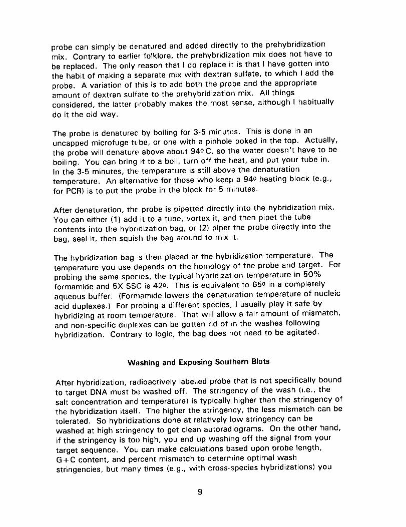
probe can simply be denatured and added directly to the prehybridizationmix. Contrary to earlier folklore, the prehybridization mix does not have tobe replaced. The only reason that I do replace it is that I have gotten intothe habit of making a separate mix with dextran sulfate, to which I add theprobe. A variation of this is to add both the probe and the appropriateamount of dextran sulfate to the prehybridization mix. All thingsconsidered, the latter probably makes the most sense, although I habituallydo it the old way.
The probe is denaturec by boiling for 3-5 minutes. This is done in an
uncapped microfuge tlbe, or one with a pinhole poked in the top. Actually,
the probe will denature above about 94o C, so the water doesn't have to be
boiling. You can bring it to a boil, turn off the heat, and put your tube in.
In the 3-5 minutes, the temperature is still above the denaturation
temperature. An alterv_ative for those who keep a 94o heating block (e.g.,
for PCR) is to put the probe in the block for 5 minutes.
After denaturation, the probe is pipetted directly into the hybridization mix.
You can either (1) add it to a tube, vortex it, and then pipet the tube
contents into the hybridization bag, or (2) pipet the probe directly into the
bag, seal it, then squish the bag around to mix it.
The hybridization bag s then placed at the hybridization temperature. The
temperature you use depends on the homology of the probe and target. For
probing the same species, the typical hybridization temperature in 50%
formamide and 5X SSC is 42o. This is equivalent to 65o in a completely
aqueous buffer. (Formamide lowers the denaturation temperature of nucleic
acid duplexes.) For probing a different species, I usually play it safe by
hybridizing at room temperature. That will allow a fair amount of mismatch,
and non-specific duplE-xes can be gotten rid of in the washes following
hybridization. Contrary to logic, the bag does not need to be agitated.
Washing and Exposing Southern Blots
After hybridization, radioactively labelled probe that is not specifically bound
to target DNA must be washed off. The stringency of the wash (i.e., the
salt concentration and temperature) is typically higher than the stringency of
the hybridization itselt. The higher the stringency, the less mismatch can be
tolerated. So hybridizations done at relatively low stringency can be
washed at high stringency to get clean autoradiograms. On the other hand,
if the stringency is too high, you end up washing off the signal from your
target sequence. You can make calculations based upon probe length,
G+C content, and percent mismatch to determine optimal wash
stringencies, but manv times (e.g., with cross-species hybridizations) you
9

don't have all the information (especially about mismatch). For that reason,many investigators determine optimal wash stringencies empirically, usingsome broad guidelines. In general, an example of a "low" stringency wouldbe lX SSC, 0.1% SDS at room temperature. A "high" stringency would be0.1X SSC, 0.1% SDS at 65o. These are the two extremes that I typicallyuse, although it is certainly possible to go lower or higher. Washes done atstringencies between these extremes will show varying levels of signalstrength and "noise" level. The washes can be done in the following way:
1. Make up your wash buffer and pour about 100-200 ml into a containersuch as a glass baking dish or a plastic container like Tupperware orRubbermaid. An alternative is to do the washes in the same bag or inanother bag. A lot of people do this, but I think it's easier to work with anopen container instead of cutting open a bag several times. There is anapparatus on the market which uses a reusable bag in which both thehybridization and washes are done. I haven't used it, so I have no opinionabout its merits. (I can say that it is expensive, however.)
2. Open the hybridization bag, squeeze out the hybridization mix, andtransfer the filter to the dish with the wash buffer. (By the way, you cansave the hybridization mix. Contrary to folklore, it can be reused. In thiskind of hybridization, very little probe has actually hybridized to your target,and very little has renatured. So you can put it in the freezer and use it onthe next filter, as long as you don't wait so long that the radioactivity hasdwindled to an unusable level.)
3. Slosh the filter gently in the container for a few seconds to get most ofthe residual hybridization mix off. Pour off the wash buffer into the liquidwaste container, and pour in another 100-200 ml. (You have just gotten ridof most of the unbound counts. Remaining washes will have very fewcounts/ml, and after the second change, are usually within the legal limit tobe put down the drain.)
4. Put the wash container on a slow shaker at the wash temperature. Thisis usually done in a shaking water bath, because the heat transfer is rapid.If you do it in a dry shaker, it's advisable to preheat the wash buffer to thedesired temperature. Of course, if your wash is being done at roomtemperature, you can just put it on an orbital shaker on the bench top. Theshaker should oscillate just fast enough to gently slosh the filter back andforth in the buffer. It's debatable how necessary the agitation is, but itcertainly doesn't hurt.
5. Generally two or three wash buffer changes, shaking about 20 minutesfor each change, is sufficient. It doesn't seem to hurt anything to overwashthe filter. I have frequently left the thing shaking all afternoon.
10

6. After the final wash the filter can be taken out, blotted on a paper towel,and sandwiched in Saran Wrap. If you intend to wash the same filter at ahigher stringency after the first film exposure, or strip the filter later andhybridize it with some other probe, it is not advisable to let the filter dry out.No filter that I know ot can be efficiently rewashed after it is dry, and sometypes of filters (e.g., Nytran) are very difficult to strip after they are dry.That's why I put it in ,(;aranWrap immediately. There are a lot of caseswhere you may want !o step up the wash stringency on the same filter,checking the signal at each stringency. So as _Jgeneral rule, don't let thefilter dry.
7. The filter can now 3e exposed to X-Ray film. I do this by mounting thefilter to some sort of backing (a piece of cardboard, an old piece of X-Rayfilm, etc.) that is the ,,_amesize as the film, so it won't move around insidethe exposure envelope. Usually, you should put some sort of marker on thefilter that will expose the film at that spot, allowing you to orient yourselfwhen you look at the developed autoradiogram. Some people useradioactive ink (a litth; 32p mixed with India ink) or fluorescent ink (whichyou can buy) and put a little mark at the top of the filter. I use little
fluorescent stickers (look in a toy store, or the children's section in a
drugstore or card shop. You can also use fluorescent star charts). Expose
the sticker to light to charge it up, then stick it to your filter. I use clear
tape to do this, so I can reuse the stickers. The fluorescent stickers are
much better than radioactive ink, because the_/give you the same signal, no
matter how long or short you do the exposure (the fluorescence dies down
after a few minutes) Besides, the less radioactivity you have to keep
around the lab, the _,etter. After the filter and its fluorescent marker are
ready, put it in an e>posure envelope and go into the darkroom. Be careful
about the kind of safelight you're using. Be sure it's rated for X-Ray film, or
you'll fog your film. If in doubt, do a trial exposure of the safe light on
blank film to see if it fogs. Alternatively, it's perfectly possible to do the
whole thing in total darkness. Open up the envelope and lay it in front of
you. Open the film box, slide out a sheet of film, and put it directly over the
filter. Before you d_ anything else, close the. film box. Almost everyone at
one time or another forgets to do this before turning the lights on. The
result is that the en,Js of the film get exposed to light, and all of them will
lose an inch or two of usable exposure area. (And the film is expensive).
Next (if you are usi_g one), put an intensifyir_g screen over the film.
(Intensifying screens are optional. They speed up the exposure time.) Close
up the envelope an.:] turn on the lights so you can find the doorknob.
8. The exposure can be done at room temperature, but it's faster at -70o,
because of reciprocity. In any event, it's usually a good idea to squish the
envelope together _ightly so the exposure is sharp. If there is any space
between the filter and film, the signal comes out fuzzy. This can be done
11
with a heavy weight like a lead brick or a phone book or some such thing.Alternatively, you can sandwich the envelope between two thick pieces ofglass or lucite and clamp them together with large binder clamps (obtainableat a stationery store). A more expensive alternative is to abandon exposureenvelopes completely and instead use metal exposure cassettes, which havetheir own clamps. (Unfortunately, they are currently about $100 apiece, asopposed to just a few dollars for cardboard exposure envelopes.) Theexposure time depends entirely upon how hot the filter is. Some exposurescan be done in less than a half hour, while others may go for a week ortwo. Your best bet if you are unsure is to let it expose overnight. If it'stotally overexposed when you develop it the next day, try it again for just afew hours. If you don't see much of a signal, let it go a few days. A weaksignal won't be much better unless you substantially increase the exposuretime. Doubling the time doesn't necessarily help that much, so I usually atleast quadruple the time.
To develo0 X-Ray Film
1) Slide or clip film into hanger (depends on the hanger)
2) Submerge in developer for 3 to 4 minutes3) Lift out and drain for 5 to 10 seconds
4) Submerge in stop bath for 10 to 20 seconds
5) Lift out, drain 5 to 10 seconds
6) Submerge in fixer for 3 to 4 minutes
7) Lift out, drain 5-10 seconds, run under water in tank for 5-10 minutes
8) Hang up to dry
12
Colony Hybridization
There are several ways of processing membrane filters containing bacterial
colonies or phage plaques. The following is probably the most popular. It
was developed by Hanahan, and can be found in the Maniatis book.
I find that the proced,Jre of "lifting" the colonies from the plate works better
if the plate is cold. 30-60 minutes at 40 is long enough. (If the plate is
warm, the colonies h,]ve a greater tendency to smear.} Using a gloved hand
or a pair of forceps, lay the membrane filter on the plate containing the
colonies, making contact with the entire surfac-e and allowing it to wet
completely. Nytran wrinkles more easily than nitrocellulose, so try to be
careful to either lay (_own the filter slowly from one edge, or bend it in such
a way that the middle of the filter makes contact with the agar first, after
which you let the edges go. If the filter wrinkles, don't try to fix it. It isn't
a serious problem, arid trying to straighten the wrinkle is likely to smear the
colonies. However, it's OK to gently run your gloved finger around the
surface of the filter to get rid of any bubbles. After it is completely wet
(usually 15-30 secords), lift the filter off of the plate with a pair of forceps.
At this stage, you c_n immediately lyse the colonies and proceed with the
prehybridization. Allernatively, you can amplify the colonies by laying the
filters, colony side u__, on new plates, allowing them to incubate for a few
hours. The latter m_.,thod gives stronger hybridization signals because there
is more cell material on the filter after amplifying them.
Colony lysis:
1. Lay out a piece of plastic wrap (e.g., Saran Wrap or Handiwrap).
2. Make a 0.75 ml puddle of 0.5 M NaOH on the plastic wrap, and carefully
lay the filter, colony side up, on the puddle. The filter will wet, and the
NaOH will lyse the colonies. Leave the filter for 2-3 minutes.
3. Lay the filter on =] paper towel to blot it dry (10-20 seconds; it doesn't
have to be d__LY_;you just need to get rid of the excess NaOH)). Don't touch
the colony side, or you'll smear the lysed colonies.
4. Next, lay the filter on a 0.75 ml puddle of 1 M Tris-HCI (pH 7.4). Thisneutralizes the filter after the NaOH treatment. Leave the filter for 2-3
minutes.
5. Blot the filter dry as before on a paper towel.
6. Lay the filter on a 0.75 ml puddle of 0.5 M Tris-HCI (pH 7.4), 1.5 M
NaCI. Leave for 2-3 minutes.
13

7. Rinse the filter by immersing it briefly (a few seconds is enough) in asolution of 5X SSC.
8. Blot the filter on a paper towel as before, and then let it air drycompletely (30-60 minutes).
9. At this stage, the filter can be processed in exactly the same manner as a
gel blot (baking or UV crosslinking, prehybridization, and hybridization).
14

The Polymerase Chain Reaction (PCR)
This procedure is one of several variations on the basic techniques
described by the Perkin-Elmer Cetus Corporation in their kit. There is
nothing wrong with b_ying their kit, but we find that it is cheaper to buy the
enzyme and make up our own 1OX buffer and dNTP solutions.
This procedure is writlen with the assumption that the template DNA is
present in a concentration of approximately 100 ng/#l. A fairly wide range
of template concentrations will result in about the same amplification, but
this is a case where more is not necessarily better. You can sometimes
improve the quality or the yield of a PCR amplification by decreasing the
amount of template DNA.
1. Mix together in a C.5 ml microtube:
H20 68.5 /_1
IOX buffer 10 #1
primer #1 2 #1
primer #2 2 /_1
template DNA 1 /_1
2. Mix by flicking the tube with your finger, then spin for a few seconds in
the microfuge to bring all the solution to the bottom.
3. Float the tube in a ,_an of boiling water for 5 minutes.
4. Remove from the boiling water and let cool for 2 minutes at room
temperature.
. While the tube cools, mix together:
16 /_1 of dNTP solution
0.5 #1 of Taq Po ymerase (2.25 units)
6. Add 16.5/_1 of dNTP/Taq Polymerase to the cooled tube. Flick to mix,
and spin briefly in the rnicrofuge to bring the solution to the bottom.
7. Add 3 drops of mineral oil ('100/_1) with a transfer pipette.
8. Put the tube in the thermal cycler and proceed with the first primer
extension (2 minutes a_: 72o).
. Continue the cycles as follows:
1.25 minutes at 940
2 minutes al 370
2 minutes at 720
15

Do this for 28 cycles (for a total of 29 primer extensions). On the 30th
primer extension, increase the time to 7 minutes. This is a ridiculously long
time, since the polymerase travels at a rate of a least 750 nucleotides per
minute. However, it assures that the last primer extension is absolutely
complete.
When the 30 th cycle is finished, the products can be checked on a minigel.
The simplest thing to do at this stage is to put a pipet tip through the oil
layer into the aqueous layer, and suck up 5 #1. Put this drop on a piece of
Parafilm, add 1 #1 of gel loading dye, mix by sucking up and down a few
times, and load onto a minigel. Alternatively, you can pipet off the oil layeror extract with chloroform to remove the oil. (Remember that chloroform is
heavier than wate_when you remove the layer.)
Cloning PCR Products into Single-stranded Bacteriophage
There are several ways of getting PCR products into a form that can be
sequenced. Direct sequencing is the fastest, and can be done after either
symmetrical or asymmetrical amplification. However, although some people
have great success with direct sequencing, it can be tricky, and often
seems to be template-, primer-, or even strand-specific. We elect to clone
the PCR products, which allows us to use universally workable sequencing
protocols. The additional time spent cloning (not very long, as you will see)
pays off later with the high quality of sequencing reactions that result. In
addition, cloning of the PCR products gives you a "hard copy" of the
amplified DNA that can be stored and grown up later if you need it.
Although it is just as easy to clone into double-stranded vectors, we clone
directly into the single-stranded bacteriophage M13 (which can also beisolated in its double-stranded form), because the sequencing reactions we
generate are consistently less artifact-ridden. However, it is worthwhile to
experience double-stranded sequencing, either of plasmids or PCR products,
and to make your own choice, particularly if you foresee doing a lot of
sequencing.
When cloning PCR products, the main problem is giving the amplified DNA
ligatable ends. This may seem surprising, because we envision the PCR
reaction giving nice blunt-ended double-stranded products that, logically,
should be easily ligated into a linearized cloning vector. The problem is that
apparently only a small percentage of the PCR products in a mixture are
truly blunt-ended. There are basically three ways to deal with this:
1. Engineer restriction sites into the primer sequences, so that the PCR
products can be digested, generating ends that will ligate to the
appropriately digested cloning vector. The trick here is to add some extra
16

"junk" nucleotides (usually 4 or more) to the 5' ends of the primers. Mostrestriction enzymes need a little extra DNA outside the actual recognition
site to hang onto in order to cut efficiently. This procedure has a lower
efficiency than you would logically expect, but we used it for a couple of
years with reasonable ,'mccess, so it's worth considering.
2. The Invitrogen company recently came out with a procedure they call
"TA cloning." The ragged ends generated during the PCR reaction are a
property of thermostable polymerases, which often add an extra A on the
end of the sequence, invitrogen has taken advantage of this by making a
vector with an extra T at the ends, complimentary to the extra A on the
amplified DNA. According to their procedure, you simply add your amplified
DNA to the already-prepared vector with its T overhang, ligate it, and
transform the cells they supply. We tried this out of curiosity and had
reasonable success. However, we found that il is almost always necessary
to gel-purify the PCR product in order to prevent cloning of shorter and
longer "background" products which, although often invisible on a gel,
show up with surprising frequency in the resulting clone bank. Another
drawback is that the cloning efficiency (by comparison with the procedure
we now use) is pretty low. There is a high background of non-recombinant
clones, but you can live with the background since the non-recombinants
have beta-galactosidase activity which is easily assayed. The kit (which
supplies everything you need) is expensive, bu_ it works.
3. "Polish" the ragged ends with a DNA polymerase, which creates good
blunt ends that can be easily ligated to a blunt-ended vector. This is the
procedure we currently use. The traditional polymerase to use is the
Klenow fragment of DNA Polymerase I. However, it has been found
(Biotechniques 9:710 [1990]) that T4 DNA Polymerase works much better
for this procedure. The advantages of the end-polishing procedure are that
it is relatively rapid, I_,as (in our hands, at least) .much higher cloning
efficiency than other techniques we have used, and allows you to clone
directly into a vector that produces single-strands if you choose. We use a
strain of phage M13 called Phagescript (sold by Stratagene). Although Smal
is a very common enzyme to use for creating blunt ends in the vector, we
find that we get higher efficiency if we use the EcoRV site that Phagescript
has in its polylinker.
17

Procedures:
End-polishing and gel purification:
1. After PCR amplification, add 15 units of T4 DNA (about 6/_1) Polymerase
directly to the reaction mix (100 #1).
2. Incubate 20 minutes at 37o.
3. To gel purify the end-polished PCR product, we use SeaKem agarose
(FMC Corporation). The type of agarose you use does make a difference in
ligation efficiency. SeaKem is made especially for this purpose. Make a 1%
SeaKem agarose gel with 0.5 #g/ml ethidium bromide. If available, a
preparative comb is nice to use. Otherwise, use a standard comb and loadseveral wells.
4. Add 1/10 volume of loading dye (10 #1) to the PCR mix.
5. Load the whole sample, avoiding the overlaid mineral oil as much as
possible.
6. Run the gel at 100V until the PCR product is clearly separated. This will
depend on the size of the product and the presence or absence of multiple
bands.
7. Cut the band out of the gel with a razor blade, scalpel, plastic gel knife,
or even a plastic ruler. Be careful not to cut the gel on a plastic gel plate, if
you're using a metal knife. You'll scratch the plate.
8. Rinse previously prepared dialysis tubing with TAE buffer and squeeze
out excess.
9. Clamp one end of the tubing (or tie it, which is less convenient) and slide
the gel slice into the open end.
10. With a Pasteur pipet or other small pipet, add enough TAE buffer to
immerse the slice (usually a few hundred microliters) and squeeze out any
bubbles. Clamp the other end of the tubing (or tie it).
11. Put the tubing into the gel apparatus, perpendicular to the current flow
(i.e., cross-wise, not length-wise).
12. Turn power supply on at 100V. The elution time depends on the size of
the DNA. For small fragments (a few hundred base pairs), 20 minutes is
more than enough. Large fragments (kilobases) are slower. Run it for 45
18

minutes to an hour, and check it on a UV box. Very large fragments don't
elute efficiently, so you might lose half of your sample. So try to start with
a lot of DNA. Small fragments elute quite efficiently, and we usually don'tlose much.
13. At the end of the elution, reverse the currenl for 45-60 seconds. This
pulls the DNA off the wall of the dialysis tubing.
14. Check the elution on a UV light box. If DNA is still in the gel, elute for
10 more minutes on the, original direction and check it again.
15. Use a Pasteur pipe1 to remove the buffer from the tubing and transfer it
to a microfuge tube. R_nse the tubing with an extra 100-200/_1 of TAE toremove residual DNA, _nd transfer it to the sam_, _ tube.
16. Measure the volume (this can be done easil_ by weighing the tube and
comparing the weight lo an empty tube).
17. Extract the eluted !_)NA with an equal volume of phenol/chloroform.
(FMC says that this st_.p is unnecessary with their agarose. They're
probably right, but we do it anyway to make sure.)
18. Precipitate the DNA with 1/10 volume of 3 M sodium acetate and 2
volumes of ethanol. We do this at -80o for 15 minutes. This reputedly
makes the DNA precipitate more thoroughly.
19. Spin in a cold microfuge for 20 minutes at 10,000 rpm. Wash the pellet
with 70% ethanol, then spin in cold microfuge for 5 minutes at 10,000 rpm.
20. Dry the pellet and resuspend in 30 #1 of sterile distilled water.
21. Run 1 /_1 of the eluted DNA on a gel along with known amounts of DNAmarkers in order to determine the concentration of the DNA (4/_1 SDW, 1 /_1
XC).
Ligation of polished PCR product to vector:
1. We want a 50:1 m.:_lar ratio of insert:vector. The vector (in our case) is
M13 Phagescript DNA digested with EcoRV. Cut a known amount of vector
DNA with EcoRV, the_ phenol/chloroform extract, ethanol precipitate, spin,
wash pellet, spin, dry. and resuspend. Check _.he recovery on a gel and
adjust the concentration, if necessary. We resuspend the vector at a
concentration of 20 ng/#l, and the protocol below is written for that
concentration. For olher concentrations, make appropriate adjustments. By
knowing the mass anLount and the size of both the vector DNA and the
19

insert DNA, we can calculate the molar ratio. For example, M13 is around
7.2 kilobases. The lu.__xxAfragment we are amplifying is 0.745 kilobases.
That's around a ten-fold difference in size (it's safe to approximate these
things). To get a 50 fold molar excess of insert (i.e., the amplified lu___xA
fragment), we need a 5 fold mass excess of lu____xADNA to M13 DNA.
2. Ligation mixes:
PCR ligation
insert DNA + H20 10.5 /_1
vector DNA (20 ng/#l) 2.5 #1 [=50 ng]
5X ligase buffer 4 /_1
10 mM ATP 1 #1
T4 DNA Ligase 2 /_1
Control ligation
H20 10.5 /_1
vector DNA (20 ng/#l) 2.5 #1
5X ligase buffer 4 #1
10 mM ATP 1 /_1
T4 DNA Ligase 2 /_1
3. Incubate overnight at 15o.
[stop -- hold at 4o]
4. Run 1 /_1 of each ligation mix on a minigel to check ligation.
5. Dilute the ligation reactions to 80 #1 with water. Reasons: (1) cells begin
to saturate with 10-15 ng of DNA, and (2) something in ligation reactionsinhibits transformations if not diluted.
Preperation of competent cells:
Have ready:
- YT plates, YT top agar, and YT broth.
- sterile 50 mM CaCI2.
- small sterile culture tubes (e.g., falcon tubes or 100 mm glass culture
tubes with caps),
- 2 heating blocks: one at 42o, one at 50o.
- the night before, inoculate 1 ml of YT with DH5a cells and shake
overnight at 37o.
- the day they will be used (unless they're warm already), take the YT plates
out of the refrigerator and put them in a 370 incubator to warm them up.
This is optional. We think it helps keep the top agar from gelling before you
2O

get a chance to swirl it _,round. It's debatable whether warm plates make
any difference to the cells themselves.
1. Inoculate 50 ml of YT with 1 ml of DH5a overnight culture. Shake "2
hours at 370 until O.D.sco = 0.3 to 0.4.
2. While the cells are growing, chill as many 50 ml sterile centrifuge tubes
(e.g., "blue caps," "orarge caps," or sterile Oakridge tubes with caps) as
you need (one per transformation), and 50 ml of .';terile 50 mM CaCI2 on ice.
3. Also while cells are growing, melt the top agar and cool it to 500. We
divide top agar into 3 m aliquots in 100 mm glass culture tubes when we
make it up. That way, (in the day of the transformation, we melt as many
as we need in a beaker ,_f boiling water, then put them in a 50o heating
block until they are used. An alternative is to have the top agar in one flask
at 50o and pipet it into 1he transformation mixes (3 ml each) before pouring
onto the plates.
4. When the cells are grown up, put them on ice for 20 minutes.
5. Pellet the cells at 5000 x g for 5 minutes in a cold centrifuge (4o).
6. Pour off the supernalant and drain as well as possible, then resuspend in
50 mM CaCI2, 1/2 origi_}al volume. Gently swirl to resuspend; the cells are
fragile in this solution.
7. Let the resuspended cells sit on ice 20 minutes.
8. Pellet the cells again 5000 x g, 5 minutes. Decant as before.
9. Resuspend the cells n 50 mM CaCI2, 1/20 of original volume, again with
gentle swirling. The cells are now competent for transformation.
10. For each transformation, add 300 #1 of competent cells to a chilledsterile culture tube.
Transformation:
Label as many chilled tubes of competent cells as you need. Also, make
sure you label all of your plates appropriately, either before or during the
transformation, so the_ will be ready when the transformation is complete.
1. We will transform with 3 different amounts of each ligation mix: 0.1 /_1, 1
/_1, and 10/_1. We are likely to get the plaque density we want on one of
21

the lower two dilutions. It's not easy to pipet 0.1 #1,so take 1 #1of ligationmix and dilute it (in SDW or TE) to 10/_1 so that you can pipet 1 /_1 of it.
2. To chilled tubes containing 300 #1 of competent cells, pipet:
1 /_1 of 1/10 diluted ligation mix
1 #1 of ligation mix
10#1 of ligation mix
Swirl the tubes gently to mix.
3. Return the tubes to ice for 30 minutes.
4. After 30 minutes, heat shock the cells at 42o for 2 minutes. (This is
done by moving the tubes to the 42o heating block for 2 minutes.)
5. To each tube, add:
50/_1 2% X-Gal in dimethylformamide
10#1 100 mM IPTG
IPTG is an inducer and X-Gal is an indicator for beta-galactosidase activity.
We are cloning into a site that interrupts the beta-galactosidase gene and
therefore knocks out its activity. X-Gal turns blue if beta-galactosidase is
active; therefore, we are looking for colorless plaques as an indication that
our insert DNA is present.
6. Pour 3 ml of 50o top agar into a tube, swirl briefly to mix, then pour onto
a YT plate. Gently swirl the plate to spread the top agar. Repeat for all
samples.
7. Let the top agar solidify ('10 minutes should be enough), then invert the
plates in a 37o incubator and leave them overnight.
8. In anticipation of growing up the clones on the following day, inoculate 1
ml of DH5a cells and shake overnight at 37o.
9. Using sterile Pasteur pipet, pull out isolated plaques (about 10 plaques, 1
per tube). Can store plug in TE at 40.
10. Blow out into 1.5 ml of DH5a cells in a culture tube. (They were diluted
1/50 from overnight culture.)
11. Shake at 37o for 6 hours.
22

Preparation of M13 Sequencing Templates
1) Use a sterile Pasteur pipet to pull an agar plug containing a single
isolated colorless plaque from the plate. Transfer the plug to a 1.5 ml
miniculture containing _ 1:50 dilution of the overnight culture of host cells
(inoculated the night before).
2) Shake for 6 hours at 37o.
3) Transfer the miniculture to a 1.5 ml microfuge tube and spin out cells for
5 minutes at full speed.
4) Carefully (i.e., withuut stirring up the pellet) lransfer 1.2 ml of the
supernatant to a fresh l ube. Save the pellet and the residual supernatant in
the original tube to use as a future inoculum. It can be stored at 40.
5) The supernatant contains the single-stranded M13 phage particles from
which you will isolate DNA. Add 300/_1 of 20% PEG (polyethylene
glycol)/2.5 M NaCI, vortex briefly, then let sit for 15 minutes at room
temperature.
6) Spin 15 minutes at full speed in the microfuge. The pellet contains the
precipitated phage.
7) Carefully pour off the supernatant. The pellet is unstable, and you don't
want to lose it. Spin tl_e pellet again briefly and use a pipet to remove any
remaining supernatant.
8) Resuspend the pellet in 100/_1 of TES by vortexing.
9) Extract with 75/_1 phenol/chloroform. Vortex 15-30 seconds, then spin
for 2 minutes in the microfuge at full speed. This strips the coat protein
from the phage, leaving the single-stranded DNA.
10) Pull off the top (aqueous) layer and transfer it to a new tube. Extract it
with 75 #1 of chloroform, then spin 2 for minutes at full speed in the
microfuge.
11) Pull off the supern_tant and transfer it to a new tube. Precipitate the
DNA with 9 p.I of 3 M _odium acetate plus 200 _1 of ethanol.
12) Spin for 20 minutes at 40.
13) Carefully pour off [he ethanol supernatant, wash briefly with 300/_1 of
70% ethanol, then spi-_ again for 5 minutes at 40.
23

14) Carefully pour off the 70% ethanol and dry the pellet (either air dry orvacuum dry until no visible ethanol is left).
15) Resuspend the pellet in 10 #1of distilled water. Check the yield byrunning 1 #1on a minigel (1 #1DNA, 4 #1water, 1 #1 loading dye).
16) The DNA is now ready to sequence.
DNA Sequencing
How to Pour a Sequencing Gel:
This is by no means the only way to pour a sequencing gel. Regardless of
which variation you use, however, it is best to pour the gel before you do
the sequencing reactions, so that it is ready when your sequencing is done.
As you will see, the actual sequencing reactions don't take very long, and
you want to make sure you have a good gel ready before you start.
All of the sequencing apparatuses that I know of have a small plate and a
large plate. The small plate is a couple of centimeters shorter than the largeplate, but the same width. The small plate goes on the inside (i.e., next to
the apparatus) when you mount the plate assembly on the gel apparatus.
That way, the running buffer from the top reservoir can reach the gel,
allowing current to flow. It's obvious when you look at the apparatus.
Before you get involved with assembling the gel plates, it's a good idea to
get the gel mix started. It takes a while to go into solution, so it can be
stirring while you work on the plates.
Stock solutions:
10X TBE buffer: 0.89 M Tris, pH 80.89 M boric acid
20 mM EDTA
40% acrylamide/bisacrylamide (29:1 )
10% ammonium persulfate (This should be fresh. Some people make it upevery day, others every week.)
24

A standard 8% gel mi<:37.5 g Urea (ultra pure)7.5 ml 10X -rBE15 ml 40% _crylamide/bisacrylamide22.5 ml H20Final volume = 75 ml
Stir the gel mix on a p._agneticstirring plate. It will go into solution morequickly if you warm it (not hot, just warm).
Now for the gel plates
1. Good gels start wit_clean plates. Dirty plates result in bubbles in the gelas the liquid acrylamice is poured between the plates. To clean the plates,use a sponge and some detergent like Alconox or Palmolive. Wash themthoroughly, and rinse excessively to get rid of detergent.
2. Allow the plates to drip dry.
3. At this stage, you r_eedto "waterproof" one of the plates. Specifically,you want to waterproaf the inside of the small plate. There are people whowill tell you that you don't need to waterproof, but I can guarantee you thatyou will have fewer gels sticking to plates (disz,strous if half the gel sticks toone plate and the oth_.,rhalf to the other) if yob waterproof. The "old" wayto waterproof is to siliconize the plate using silane. It's expensive and youhave to use it in the hood. A cheap alternative is to use "Pam" (the stuffyou use to keep food from sticking to frying pans). By far the best choiceof all is "Rain-X," which you get at an auto supply store for waterproofingyour windshield. It's as good as silane, with none of the disadvantages.Procedure: Squirt eth_tnol on the small plate and wipe it down. Let it dry.Soak a Kimwipe with Rain-X and completely coat one side of the plate(make sure that this becomes the inside of the plate in the finished gelassembly). A hazy fil_-nwill form, which clears away with longer rubbing.
4. After waterproofing wash both the large and small plates thoroughly withethanol. Allow the etr_anol to evaporate after washing, then repeat about 3times for each plate (just to be thorough).
5. Wash and ethanol ,;lean the spacers and gel comb.
6. Lay the large plate on a raised surface like a styrofoam box, so you haveaccess to the entire perimeter of it.
25

7. Place the spacers along the edges and bottom of the large plate. Placethe small plate (waterproof side down) on the large plate, align the edges,and adjust the spacer if necessary to make a good seal. Clamp the platestogether using binder clips (obtained at an office supply store); 5 small clipsalong the bottom and 4 large clips along each side works well. Note: Analternative to this is to use only side spacers and to tape the gel plates
together using very thin plastic tape. Some people think this is the best
technique, but it can be tricky to tape it in such a way that the assemblydoesn't leak.
8. When the plate assembly is ready, add 450/_1 of 10% ammonium
persulfate to the acrylamide/urea mix.
9. Add 20 #1 of TEMED and immediately pour the gel mix between the
plates. The actual pouring can be done using a lar_Eg_syringe, a squirt bottle
(e.g., a laboratory wash bottle), or even a small plastic beaker. If you use a
beaker, make sure it has a sharp spout on it so that the acrylamide doesn't
dribble down the side. Tilt the plate assembly at an angle (-30-45 degrees)
and up on one bottom corner, so that the acrylamide flows down to one
corner when it is added, and slowly fills up the plate assembly. Pour
slowly, watching for bubbles. If a bubble appears, tilt the plate to the other
side and pound it out with the side of your hand. If the bubble persists, and
it is small, leave it and avoid using that lane when you load the gel. Just
circle it with a felt pen on the outside of the plate to remind yourself where
it is. If it is disastrously large, try your best to get rid of it. The problem
here is that the acrylamide will begin to polymerize in a few minutes, so youdon't have a lot of time.
10. Lean the plate back against something so that it is nearly flat, then
insert the comb. If you are using a standard comb, push it in until the
acrylamide almost reaches the tops of the teeth. If you are using a "shark
tooth" comb, insert the comb upside down (i.e., with the teeth up_) until the
teeth are 1-2 mm above the edge of the larger plate.
11. Clip in 2 places on the top of the gel to press the plates against the
comb with no air gaps. (This is a precaution against slightly warped plates,which are not uncommon.)
12. Immediately rinse out the syringe or wash bottle (if you are using one)for future use.
13. When the remaining few milliliters of gel in the bottom of the original
container have polymerized (-30 minutes or so), the gel is ready to mount inthe apparatus.
26
14. Gently pull out thc, bottom spacer (unless you taped the gel plates, inwhich case there is n¢.bottom spacer). Then pull out the comb. A standardcomb can be gently eased out of the gel, after which the wells can berinsed with lX TBE bL.ffer and straightened out. if necessary. (Sometimesthe wiggly little pieces of polyacrylamide in between the wells get bent outof shape. Be careful straightening them, because they will break.) Asharktooth comb can be ge,_tly pulled out and reinse:'ted right side up after thegel is mounted in the apparatus. You might need to clean off bits of driedacrylamide on the out;;ide of the plate, or small bits of polymerizedacrylamide from the s_mple wells.
15. Different apparatuses have different ways of attaching the plate
assembly, but most inJolve some sort of clamplng mechanism. After
attaching the plate as,,;embly to the apparatus, fill the reservoirs with 1X
TBE. After the plate assembly is mounted on tt_e apparatus and the upper
and lower reservoirs are filled, you will need to blow out the air space
created by the (now removed) bottom spacer. (Again, this is unnecessary if
you have used taped plates, because there is no spacer at the bottom.)
This procedure can be mildly exasperating, but once you get the knack of it,
it is quite easy. It can be done with a Pasteur pipet which has been bent
intoa U shape using a bunsen burner. Fill the pipet with lXTBEand
position the end so th_ht it is aimed up between the plates on the bottom.
Then squirt the 1X TB- out into the space, blowing the bubble toward one
side or the other. Keep doing this until you have chased all the air out of
the space. The gel is -low ready.
Sequencing of Single-,(;tranded M13 Clones Using "Sequenase" (Modified T7
DNA Polymerase):
Sequencing DNA usin(j the dideoxy chain termination method is
conceptually identical to sequencing RNA, although it differs in certain
details of the procedure. [NOTE: RNAsequencing is described by Dr.
Saffarini in the followin_g section of this publicalion.] A specific primer is
annealed to the temple, re, then the primer is extended with a DNA
polymerase, and the g_owing chains are terminated by addition of
dideoxyribonucleotide,,., resulting in a populatiorl of molecules of lengths
differing by a single nL;cleotide. The population of terminated chains can
then be separated on _J polyacrylamide gel, resulting in a sequencing
"ladder" from which tP_e DNA sequence can be read. There are numerous
variations on the protocol which follows. This protocol is derived from the
one that U.S. Biochemical Corporation provides with its "Sequenase" kit.
The procedure involve:_: (1) primer/template annealing in one tube, (2) a
labelling reaction (in tee same tube) using only deoxyribonucleotides
(including P-labelled dATP) in which primers are allowed to extend for a
while before terminatir_g, (3) division of the labelling reaction into 4 separate
27
tubes (A,C,G,T), (4) addition of the appropriate dideoxyribonucleotide toeach tube to begin terminating chains, and (5) stopping the reactions,followed by denaturation and loading on the gel. The details are as follows:
1. In one micro tube, add:template DNA ('1 /_g) + H20 7 ml
5X Reaction Buffer 2 ml
0.5 pMole primer (3 ng M13 primer) 1 ml
Mix by gently pipetting up and down a few times.
2. Put tube in 65o heating block for 2 minutes (to denature any interfering
secondary structure). To anneal the primer, remove the block itself from the
heating element and set it on the bench top to cool to approximately room
temperature. (An alternative to this procedure is to put the microtube in a
test tube of 650 water, put it in a 65o water bath for 2-3 minutes, then
remove the test tube containing the microtube, and let it cool.)
3. While the annealing is taking place:
A. Label
another C,To the
To the
To the
To the
(These are
4 micro tubes for the termination reactions.
another G, another T.
A tube, add 2.5 #1 ddATP
C tube, add 2.5 #1 ddCTP
G tube, add 2.5/_1 ddGTP
T tube, add 2.5 #1 ddTTP
the tubes that will be used in step 5.
Label one A,
Put aside until then.)
B. Make labelling mix dilution in a micro tube. Note: The Sequenase kit
comes with a dGTP labelling mix and a dlTP labelling mix. The dlTP mix is
used occasionally to help read through regions of compression (when strings
of C's and G's pile up on the sequencing gel). For the usual sequencingreaction, the dGTP labelling mix is used. Both mixes contain dCTP and
dTTP. The only difference between the two is that one contains dlTP
instead of dGTP. The dATP is added as the labelled deoxyribonucleotide.
To read the "normal" range (30-300 nucleotides):
1 /_1 5X dGTP mix
4 #1 H20
To read close to the primer (under "30 nucleotides):
1 #1 5X dGTP mix
14/_1 H20
28

C. Just before you'.re going to use it in step 4, dilute the enzyme
(Sequenase) 1:8 in ice-cold enzyme dilution buffer, and put it on ice.
Sequenase will last for about 60 minutes on ice after this dilution is made,
so don't do this step until you're ready to set up the labelling reaction.
4. Labelling reaction: Note: this is done in the same tube that the annealing
was done in. (i.e., there is only one tube so far). They get divided up into
separate A, C, G, and T tubes in the next step.
To the 10 #1 of annealed template/primer, add:
0.01 M DTT (dithi_)threitol) 1.0 #1
labelling mix (diluted in step 3B) 2.0 #1
32P-dATP or 35S-dATP (5/zCi) 0.5/_1
Lastly, add the diluted enzyme: 2.0 #1
Incubate the labelling mix at 20-25o for 5 minutes. Unless your lab is
unusually cold or hot, this is room temperature.
5. Transfer 3.5 #1 of the now-labelled reaction mix to each of the 4 labelled
tubes (A, C, G, T) containing the termination mixes (the ddNTP's). Heat 5minutes at 42o.
6. Stop each reaction with 4/_1 of stop solution. The samples can now be
denatured and loaded on the gel.
7. To denature (this separates the labelled ddNTP-terminated strands from
the unlabeled template strands): heat the samples to 75-95o for 2 minutes
and immediately load on the gel.
8. Loading the gel: you need to blow out the urea which has diffused into
the sample wells before loading. Otherwise, the sample will not sink into
the well. This is done most easily with a syringe with a small needle, or a
Pasteur pipet. Just squirt lX TBE from the top reservoir into the wells
(avoid creating bubbles) to blow out the wells.
9. Run the gel at 2000 volts for the appropriate time depending on your
purposes. We routinely run it 2-2.5 hours, turn off the current, load another
set of lanes, then run for another 2-2.5 hours before taking the gel off to
expose it. That way you get a "short run," allowing you to read near the
primer, and a "long run," allowing you to read far into the sequence. If it's
a good set of reactions, you can carry this to extremes by running for 8
hours or so. You can get more sequence that way, but not proportionately
more sequence, since the migration of the fragments is a logarithmic
relationship to fragment length. After a certain length, you can't resolve the
fragments no matter how long you run them.
29

Taking the Gel Off:
This is the most harrowing part of sequencing.
at this point, if you're not careful.
You can lose a perfect gel
1. Turn off the power and unplug the leads.
2. Unclamp the gel plates from the apparatus and lay the assembly down,
small plate up, on the lab bench (preferably on a sheet of benchcoat).
3. Carefully pull out the spacers.
4. Using a thin spatula or other such tool, gently pry the plates apart. If the
waterproofing has worked properly, the small plate should come free of the
large plate.
5. What you do at this point depends on whether you are exposing the gel
wet (an option only if you are using 32p) or dry. The easiest way to deal
with a wet gel is to lay a used piece of X-Ray film on top of the gel, make
sure it makes good contact with the whole gel surface, and then carefully
pick it back up. The gel should come with it. You then lay Saran Wrap
over the gel, smooth it out, and take it in the dark room and expose it. If
you are going to dry the gel, lay a large piece of filter paper (e.g., 3MM)
over the gel and smooth it out. Slowly pick it up from one end, checking
underneath to make sure the gel is coming up with it. If it isn't, lay it back
down and try again. When you have successfully lifted the gel off the
plate, put it on the gel dryer, cover it with Saran Wrap, lay the rubber sheet
over it, and turn on the vacuum. It might take both hands (and sometimes
more) to hold the rubber sheet down until the vacuum grabs. We use a
large piece of plexiglass cut to the size of the gel dryer to hold it down.
When the vacuum takes hold, turn the heater to 60-80o and let it dry for a
couple of hours. (You can let it go overnight if you don't mind running your
vacuum pump that long.) After it's dry, take it in the dark room and expose
it. Popular mythology says that you can't expose a 3sS gel with Saran Wrap
on it. Untrue. Although Saran Wrap decreases the signal from 35S
somewhat, it is not a big problem. We use Saran Wrap and easily read
them the next morning. The advantage to Saran Wrap is that the film
doesn't stick to the gel, which sometimes happens in humid weather.
Another popular myth is that you must "fix" gels by soaking them for 10
minutes in 10% methanol, 10% acetic acid before drying them. Here's the
real story: Fixing the gel gets rid of the urea. That makes the gel less
sticky, so the problem of film sticking in humid weather is lessened. It also
makes it easier to get the gel off the plate with 3MM. It is not true that
urea kills the 3sS signal. Like Saran Wrap, it may lower the signal a bit, but
it's not a big problem. We routinely leave the urea in 35S gels. Since we
also "break the rules" by leaving the Saran Wrap on, sticking is no problem.
30
More Comments:
Dideoxy sequencing is generally easier than the alternative (chemical
sequencing, also known as "Maxam-Gilbert" sequencing), so it is by far the
most popular method. The two techniques have their own set of potential
artifacts, so it is hard to say which is "better" overall, although some labs
routinely use chemical sequencing for very shc}rt fragments that must be
read with absolute at'curacy. Dideoxy sequencing is best for reading long
sequences. Because several primers can be used on the same template
(although not at the ,.same time, unless you're using a method that allows
you to distinguish between superimposed sequencing ladders), you generally
need only one or a few relatively large templates to sequence an entire
gene. With the availability of small "consumer-scale" automated
synthesizers, the ideal scenario is to sequence a large template until you
can't read any farther (about 250-400 nucleotides in an average reaction),
then back up about 50 nucleotides and design a new sequencing primer
based on the sequen('e you've just read. The new primer can then be used
to read the next 250-400 nucleotides, etc. If you're sequencing cloned
templates in any of the commercial plasmid or M13 vectors, the
manufacturer can seil you a "universal" sequencing primer which will anneal
just outside the polytinker (i.e., the cloning site). Custom internal primers
can be made afterw_rd based on the sequence read from the universal
primer. If you're sequencing PCR products, you can start with the PCR
primers themselves, each in a separate reaction. (Of course, if'you're
sequencing PCR products which have been cloned into M13, only one PCR
pr;mer will work on _ given clone, since they're single-stranded.) A
cautionary note is that uncloned PCR product._ are notoriously difficult to
sequence and should be meticulously free of the original PCR primers, so
that you don't end up priming sequencing reactions in opposite directions atthe same time.
Many (but not all) of the artifacts associated with dideoxy sequencing can
be attributed to secc, ndary structure in the template or the products.
Sequencing artifacts are frequently dealt with by:
1. Using alternative _ieoxy analogs like dlTP or 7-deaza-dGTP, which help
prevent compressior,.
2. Using a different _nzyme and/or reaction temperature. Originally, Klenow
was the most frequently used enzyme, but Sequenase has gained popularity
because it generally reads slightly better. Reverse transcriptase (used at 42-
50o) can be used equally well on RNA or DNA templates. It can read
through certain regions better partly because of the elevated temperature.
More recently, Taq polymerase has been used to help straighten out
secondary structure Because Taq polymerase has an optimum of 72o, most
template secondary structure is eliminated. laq polymerase has also been
31
used in a "cycling" sequencing reaction which results in linear amplificationof the products. The reaction is reminiscent of PCR, but with only oneprimer.
3. Often, starting with a different primer that still allows you to cover the
same region can help read through difficult spots. Better still, reading the
other strand (an option available only with DNA) usually takes care of the
problem, since opposite strands almost never form the same type of
secondary structure. Some journals (for example, Nucleic Acids Research)
require sequencing of both strands of DNA.
The use of 32p has the advantage of giving you red-hot sequencing ladders
that can be exposed and read in a very short time (sometimes 2 hours or
less). The gel can be exposed wet, although the bands are correspondingly
fuzzier because of the increased distance the beta particle travels before
hitting the film. 32p-labelled sequencing products must be loaded on the gel
right away (i.e., the same day), because their quality rapidly declines if they
are stored. They are noticeably less distinct after as little as one night at -
20o. 3sS generally gives more readable gels because it yields sharper bands.
In addition, the sequencing products can be stored at -200 for days without
loss of quality in the bands. This can be a real advantage, since the gels are
fragile and occasionally you wreck them in one way or another. When that
happens, it's nice to be able to make a new gel the next day and run the
samples again. The disadvantage of 35S is that its lower energy requires a
dry gel and a longer exposure time than 32p.
In general, the sequencing of single-stranded DNA yields more readable gels
than double-stranded DNA. In turn, double-stranded DNA templates
generally yield more readable sequences than RNA. PCR products are
variable. You may run into people who are able to get gorgeous sequences
from double-stranded templates, PCR products, or even RNA, comparable to
the quality of single-stranded DNA. But such cases are in the minority, and
they are often very sequence-dependent. Some genes just work better thanothers.
Sequencing technology is advancing at a rapid pace, and I suspect that in
10 years or so, even "small-time" labs will be able to send their templates to
"centers" to have them done in automated sequencers. We are almost
certainly the only generation who will do this manually. For the present,
however, this is what we do. If you foresee doing a lot of sequencing, keep
your eyes and ears open for new variations. All of the biotech companies
that sell sequencing supplies send out periodical newsletters describing their
latest improvements. Some are of dubious worth, but you might run across
one that improves the quality or rapidity of your sequencing.
32

Clas._,ification of Bacteria Using 16S rRNA
For the classification of bacteria, sequences of either 5S or 16S rRNA
can be used. However, 16S rRNA is longer than the 5S rRNA molecule, and
therefore provides moJe information. Two major methods are currently used
for RNA sequences. 1he first involves the use of 16S PCR products, and
the other involves dire3t sequencing using the reverse transcriptase, which
is the protocol that w_ are going to use.
1- Sequencing RNA using PCR. Two primers are used to generate an
almost full length 16S rRNA product. The fragrnents can then be sequenced
either directly or by subcloning into M13. This method is useful when you
are trying to identify organisms that cannot be cultured in the lab.
2- Sequencing using =everse transcriptase. Total RNA is extracted and the
16S rRNA is sequenced using primers that are ,,;paced approximately 300
bases apart on the RNA strand. The reverse transcriptase will synthesize a
DNA strand that is cofnplementary to the RNA, in a reaction similar to that
used in cDNA synthesis. Several primers are u.';ed that are approximately
350 bases apart. The sequencing protocol that we are using is the dideoxy
sequencing procedure (Sanger and Coulson).
RNA extraction:
- Grow a 50 ml culture: overnight.
- Centrifuge the cells at 6000 rpm for 25 minutes. Resuspend the cells in 1
ml of Tris/Mg acetate.1 mM Tris-HCI
10 mM Mg actuate
pH 7.4- Vortex
- Add an equal volume, of 70% phenol (70% phenol, 30% distilled water) todenature the RNase.
- Shake cells vigorousiy for 10 minutes.
- Centrifuge at 6000 rpm for 10 mins. Aqueous phase (top) contains RNA.
- Transfer top phase t a clean tube, and extract once with one volume of TE-
saturated phenol/chloroform (1:1). Centrifuge.- Transfer top phase to a clean tube and extract once with an equal volume
of chloroform. Centrifuge.
- To top phase add 1/10 volume 3 M KOAc pH 6.0 and 2 volumes of
ethanol. Shake. Keep at -20oC for 1/2 to 1 hour.
- Centrifuge RNA at 8000 rpm for 10 minutes.
- Resuspend in 100/_1 DEPC-treated water. Keep at -200.
33

Quick Gel:
0.4 g 1% agarose40 ml TEA buffer
cool to 55o
3 #1 EtBr (Ethidium Bromide)
40 /_1 Proteinase K (10 mg/ml)Use Hind marker; should see three distinct bands 23, 16, and 5.
RNA sequencing:
We are using one primer for sequencing, 1392r. The numbers of the
primers correspond to the positions of the primers on the E. coli 16S rRNA.
1. Anneal RNA to primer:
to an RNase free eppendorf tube (0.5 ml) add:
5-7 #g RNA
1.4 #1 reverse transcriptase hybridization buffer
1 #1 primer (100 ng)
Heat at 85oC for 5 minutes, then transfer immediately to 48oC.45 minutes.
Incubate for
2. Prepare reaction tubes. Label four 0.5 ml eppendorf tubes G, A, T, C.
Add 2.5 #1 of the appropriate mix to each tube.
3. To annealing tube add:
3.5 /_1 5X RT buffer
2.5 #1 32-P-dATP (400 Ci/mMole)
4 /_1 RT (diluted 1:5 in RT dilution buffer)
Mix and add 3 #1 to each of the reaction tubes in step 2.
4. Incubate at 50oC for 15 minutes.
5. Add 1 #1 chase mix (2 mM of the 4 deoxys; change ratio of
dideoxy:deoxy, thus making it longer) to each tube and incubate further for15 minutes.
6. Stop reaction by adding 5/_1 of stop buffer. Can hold at -200. [NOTE: P-
32 products degrade after 2 days, S-35 after 1 week]
7. Heat samples at 90oC for 2 minutes to denature, before loading on gel.Nucleotide Mix:
250 #M dCTP
250 FM dGTP
250 #M dTTP
62 #M dATP5X RT buffer to a final concentration of lX.
34
Prepare 4 tubes of the above mix and label A, G, T, C.to A tube add: 50 #M ddATP
to C tube add: 60/_M ddCTP
to G tube add: 60 #M ddGTP
to T tube add: 60 #M ddTTP
RT hybridization buf'er (5X):
0.25M Tris-HCI pH 8.30.1 M KCI
RT buffer (5X):
0.25 M Tris-t4CI pH 8.50.05 M DTT
0.05 M MgC2
RT dilution buffer:
50 mM Tris-HCI pH 8.32 mM D'I-T
50% glycerol
I OX TBE buffer:
1 M Tris-b,_se
1 M boric acid
20 mM EDTApH 8
Acrylamide/Bisacrylamide:
38 g acrylamide
2 g his-act ylamide
up to 100 ml water
8% sequencing gel
36 g urea7.5 ml IOX 1BE
15 ml acrylamide
Heat at 500 until melted, then cool at 40 for 15 minutes.
up to 75 ml with distilled water.
450 #1 10% ammonium persulfate
20 #1 TEMED
[NOTE: on 8% gel: bromphenol blue migrates as if about 20 bases, xylene
cyanol -80 bases. On a 6% gel: migration of bromphenol blue "40 bases,
with xylene cyanol approximately 100 bases.]
Stop Buffer:45% formar-_ide
20 mM EDT/k pH 8.00.05% BP Blue
0.05% Xylene cyanol
35

cDNA Cloning Protocols
Prepared by: Thomas T. Chen and Chun-Mean Lin
Center of Marine Biotechnology, Univ. of Maryland
Contents:
Extraction of Total _,NA and Poly-(A) +-RNA
Construction of cDNA Library
Preparing High Specific Activity Single-Stranded cDNA Probes
Transfer of Nucleic Acids to Nylon Membrane
and Conditions for Hybridization
DNA Sequencing with T7 DNA Polyrnerase (Sequenase)
Polyrnerase Chain Reaction Assay Conditions
Preparation of Single-Stranded cDNA Synthesis for PCRCloning of DNA from PCR Amplification
Strategies for Cloning and Characterizing cDNA
Appendix 1: RACE
Appendix 2: Screening a cDNA Clone by Irnnrnunochernical Methods
Appendix 3: Amplification of the Larnbda Zap-II Library
Appendix 4: Extraction of High Molecular Weight DNA
37
43
51
53
56
61
64
64
66
86
89
91
92
36

I. EXTRACTION OF TOTAL RNA AND POLY-(A) +-RNA
Ao METHOD I: EXTRACTION OF RNA FROM PITUITARIES AND
LIVERS OF RAINBOW TROUT BY PHENOL-CHLOROFORM-SDS
• Mix the following in a RNase-free tube:
lX extracticn buffer* 10 ml
10% RNase free SDS 1 ml
Vanadyl Ribonucleosides Complexes 0.5 ml
Polyvinyl SL_lfate (25 mg/ml) 20 pl
Spermine (35 mg/ml) 20 pl
/3-mercapto(_thanol (100%) 500 pl
2. Add 1 gram tissue to the above solution. Homogenize the
mixture in an H202 treated tissumizer.
3. Add 10 ml of phenol saturated with 1x extraction buffer to the
tube and sha<e vigorously for 10 min.4. Add 10 ml of chloroform and shake for another 10 min at room
temperature•
5. Centrifuge at 4000 rpm for 10 min in a table top centrifuge to
separate the .;Jqueous and organic phases.
6. Pipet out the organic phase carefully and do not remove the
interphase.
aqueous layer (DNA andRNA)
interphase
phenol-chloroform layer
.
8.
9.
10.
Repeat steps 4-6 several times until tP,e interphase becomes
minimal (or does not change volume anymore).
Add 1/10 vol. of 3 M NaOAc (pH 5•2) and 2.5 vol. of ETOH to
the tube. Leave the tube at -20oC for 2 hrs (or overnight).
Centrifuge at 10,000 rpm for 10 min at 4oC.
Discard supernatant and resuspend the pellet in 10 ml of 3 M
NaOAc (pH 5.2)• This precipitates the RNA, and the high
molecular w(_ight DNA remains in the aqueous phase.
37

11.
12.
13.
14.15.16.
17.
Repeat steps 9-10 several times (depending on the amount ofglycogen in the sample).
After final centrifugation, dissolve the pellet in 5 ml of 20 mMEDTA (pH 8.0) and leave it at room temperature for 10 min.Extract with phenol, then chloroform and precipitate the RNA
with ETOH.Rinse with 70% ETOH and dry in the speed vacuum.Resuspend pellet in an appropriate volume of RNase-free H20.Make a 1/100 dilution of the RNA solution and determine theconcentration in the spectrophotometer. One unit of A26 o =
40 pg of RNA.
Determine the purity of the RNA by running a gel with boratebuffer.
NOTE:
*IX RNA extraction buffer:
100 mM NaOAc (pH 5.0)25 mM NaCI
35 mM MgCI2
25 mM EGTA
38

g. METHOD I1: GUANIDINIUM THIOCYANATE METHOD FOR RNA
EXTRACTION
(a) Reagents:
(1) GT bfffer (pH 7.6); the solution must be filtered.
gL_anidinium thiocyanate 4 MTris 20 mM
_-mercaptoethanol 1 M(NOTE: Add /_-mercaptoethanol just before use)
(2) GC buffer (pH 7.0); the solution must be filtered.
Guanidinium hydrochloride
Sodium acetate
Na-EDTA
8M
20 mM
20 mM
(3) 4 M sodium acetate or potass,um acetate (pH 5.2)
(b) RNA extraction:
1. 1 gram c_f animal tissue in liquid r4trogen powder form is
vigorously homogenized in a blender with 10 ml of GT
buffer for 2-3 min. The homogenate is centrifuged at
10,000 -pm for 10 min at 4oC. "[he supernatant is
collected in a separate tube.
2. Adjust the supernatant to pH 5.2 with a few drops ofconcentrated acetic acid. Add 0.5 vol. of 95% ETOH
and leave it at -20oC for 30 min.
3. Collect the precipitates by centrif,Jgation at 12,000 rpm
for 20 rain. Dissolve the pellets i_l GC buffer (5 ml GC/1
gm fresth tissue).4. Add 0.5 vol. of ETOH and leave the mixture at -20oC for
30 min.
5. Repeat ,,_teps 3 and 4 at least twice.6. Dissolve the pellets in 20 mM EDFA (2 ml/1 gm tissue)
and vorlex to resuspend the pellet (you will not get a
clear solution at this step). Add 3 vol. of 4 M sodium (or
potassium) acetate to the solution (to make the finalconcentration of the mixture 3 M). The mixture is left at
-20oC f(,r 30 min. This step replaces guanidinium salt
with sodium or potassium salt in the RNA, and also
washes away DNA and tRNA from the RNA sample.
Collect 1he RNA pellet by centrifugation at 12,000 rpm
39
for 20 rain. Repeat this step several times.7. Dissolve the pellet in RNase-free H20. Centrifuge the
sample at 8000 rpm for 10 min to remove theundissolved material. The RNA is recovered from thesolution by precipitation with 2.5 vol. of cold ETOH and1/10 vol. of 3 M sodium acetate.
8. Recover the RNA by centrifugation. Wash the pellet in70% cold ETOH. After drying down the pellet, dissolvethe RNA in appropriate volume of RNase-free H20.Determine the concentration by spectrophotometer.
40

C. ISOLATION OF POLY-(A)+RNA BY OLIGO-d(T) COLUMN
CHROMATOGRAPHY
(a) Buffers:
(1) 1X bir_ding buffer:
10 mM
0.SM
1 "nM
0.1%
HEPES (pH 7.5;LiCI
EDTA
SDS
(2) Elutiorl buffer:
10 mM
1-nMHEPES (pH 7.5',EDTA
(b) Procedures:
1. Swell .Jp oligo-d(T) cellulose in 1X binding buffer
(1 g/30 ml) at 4oC overnight.
2. Plug tl_e tip of a 1 ml pipette tip with siliconized glass
wool, then pipette in about 0.6 ml of oligo-d(T)cellulose.
3. Wash the column with 5 ml of 0.5 N NaOH.
4. Wash the column with 1X binding buffer extensively
until tt_e pH of effluent become:{ 7.5.
5. Add 1 vol. of 2X binding buffer to the RNA solution,heata_ 65oC for 10 min. Allow the RNA solution to
cool down.
6. Add tl'e RNA solution onto the column. Collect the
effluert. Wash the column with 1 mlof 1X bindingbuffer. Collect the effluent and combine both
effluertstogether. Heat at 65oC for 10 minandreload onto the column.
7. Collecl the effluent and precipitate RNA with ETOH.
This fraction would be poly-(A)-RNA.
8. Wash the column with 5 ml of 1X binding buffer and
allow the column to drain dry.9. Elute the column with 2 ml of elution buffer to
recover poly-(A)+RNA. Collect 0.5 ml fractions.
10. Add 1/10 vol. of 3 M NaOAc (pH 5.6), 10/1g t-RNA,
and 1 ml of ETOH to precipitate the RNA.
41
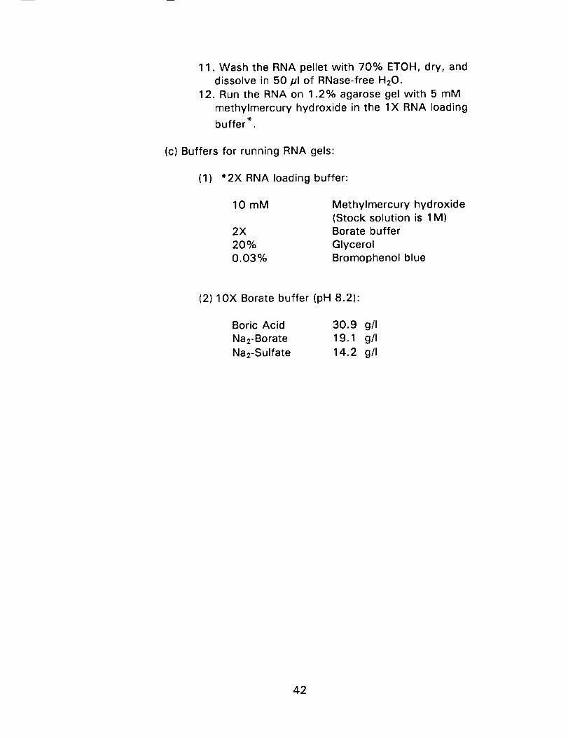
11. Wash the RNA pellet with 70% ETOH, dry, anddissolve in 50 pl of RNase-free H20.
12. Run the RNA on 1.2% agarose gel with 5 mM
methylmercury hydroxide in the 1X RNA loading
buffer*.
(c) Buffers for running RNA gels:
(1) *2X RNA loading buffer:
10 mM
2X
20%
0.03%
Methylmercury hydroxide
(Stock solution is 1M)
Borate buffer
Glycerol
Bromophenol blue
(2) 10X Borate buffer (pH 8.2):
Boric Acid 30.9 g/I
Na2-Borate 19.1 g/I
Na2-Sulfate 14.2 g/I
42

II. CONSTRUCTIOIXJ OF cDNA LIBRARY
(A) Reagents and Buffers:
a) 5X Reverse transcriptase buffer (RT buffer):
_'_50 mM Tris-HCI (pH 8.3)
50 mM MgCI2
b) 10X dXTP:
"i2.5 mM dATP
12.5 mM dTTP
12.5 mM dGTP
5 mM dCTP
c) 5X E coli DNA poll - RNase H buffer:
50 mM HEPES (pH 7.0)
25 mM MgCI2
500 mM KCI
2.00/JM each of dATP, dCTP, dGTP, and dTTP.
d) l OK Ligation buffer:
500 mM Tris-HCI (pH 7.8)
100 mM MgCI2
e) 10X Methylation buffer:
100 mM Tris-HCI (pH 7.5)2 mM EDTA
f) 5X T4 polynucleotide kinase buffer:
300 mM Tris-HCI (pH 7.8)
50 mM MgCI2
60 mM /3-mercaptoethanol (/3-ME)
g) 1C,X Core buffer:
100 mM Tris-HCI (pH 7.5)
100 mM MgCI2
500 mM KCI
100/lg/ml nuclease free BSA
h) Dilution fluid:
10 mM Tris-HCI (pH 7.4)
10 mM MgCI2100 mM NaCI
43
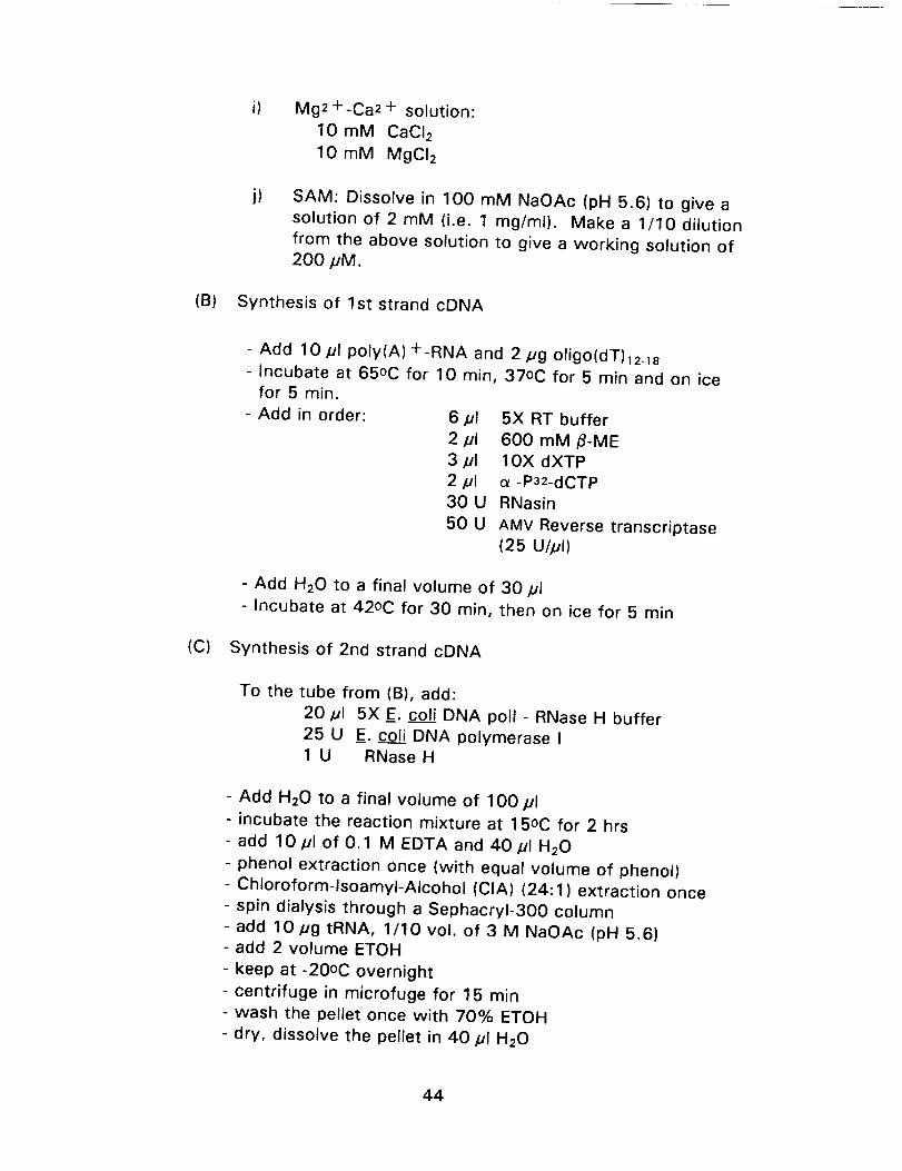
i) Mg2+-Ca2+ solution:
10 mM CaCI2
10 mM MgCI2
j) SAM: Dissolve in 100 mM NaOAc (pH 5.6) to give a
solution of 2 mM (i.e. 1 mg/ml). Makea 1/10 dilution
from the above solution to give a working solution of
200 pM.
(B) Synthesis of 1st strand cDNA
- Add 10 pl poly(A)+-RNA and 2 pg oligo(dT)12_18
- Incubate at 65oC for 10 min, 37oC for 5 min and on icefor 5 min.
- Add in order: 6 pl 5X RT buffer
2pl 600 mM/_-ME
3 pl IOX dXTP
2 pl e -P32-dCTP30 U RNasin
50 U AMV Reverse transcriptase
(25 U/pl)
- Add H20 to a final volume of 30 pl
- Incubate at 42oC for 30 min, then on ice for 5 rain
(C) Synthesis of 2nd strand cDNA
To the tube from (B), add:
20 pl 5X E. coli DNA poll - RNase H buffer
25 U E. coli DNA polymerase I1 U RNase H
- Add H20 to a final volume of 100 pl
- incubate the reaction mixture at 15oC for 2 hrs
- add 10 pl of 0.1 M EDTA and 40 pl H20
- phenol extraction once (with equal volume of phenol)
- Chloroform-lsoamyI-Alcohol (CIA) (24:1) extraction once
- spin dialysis through a Sephacryl-300 column
- add 10 pg tRNA, 1/10 vol. of 3 M NaOAc (pH 5.6)- add 2 volume ETOH
- keep at -20oC overnight
- centrifuge in microfuge for 15 min
- wash the pellet once with 70% ETOH
- dry, dissolve the pellet in 40 #1 H20
44
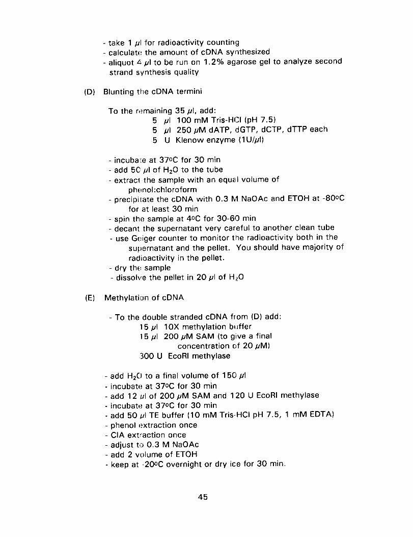
- take 1 pl for radioactivity counting
- calculate the amount of cDNA synthesized
- aliquot zz pl to be run on 1.2% agarose gel to analyze second
strand synthesis quality
(D) Blunting the cDNA termini
To the r,_.maining 35/_1, add:5 /11 100 mM Tris-HCI (pH 7.5)
5 pl 250/JM dATP, dGTP, dCTP, dTTP each
5 U Klenow enzyme (1U/pl)
- incubate at 37oC for 30 min
- add 5C/Jl of H20 to the tube
- extracl the sample with an equal volume of
phenol :chloroform
- precipi[ate the cDNA with 0.3 M NaOAc and ETOH at -80oCfor at least 30 min
- spin the sample at 4oC for 30-60 min
- decant the supernatant very careful to another clean tube
- use Geiger counter to monitor the radioactivity both in the
supernatant and the pellet. You should have majority of
radioactivity in the pellet.
- dry the sample
- dissolve the pellet in 20 pl of HzO
(E) Methylation of cDNA
- To the double stranded cDNA from (D) add:
15 #1 I OX methylation buffer
15#1 200pM SAM (to give a final
concentration of 20 pM)
300 U EcoRI methylase
- add H2() to a final volume of 150 #1
- incubate at 37oC for 30 min
- add 12 ul of 200 #M SAM and 120 U EcoRI methylase
- incubate at 37oC for 30 min
- add 50 ul TE buffer (10 mM Tris-HCI pH 7.5, 1 mM EDTA)
- phenol q_.xtraction once- CIA extraction once
- adjust t=3 0.3 M NaOAc- add 2 volume of ETOH
- keep at -20oC overnight or dry ice for 30 min.
45

- wash the pellet with 70% ETOH- dry the pellets and dissolve it in 20 #1 H20
(F) Ligation of linkers
- Add:
20 pl
5 #1
4#1
5/115U
5/11
double stranded cDNA
10X ligation buffer
EcoRI linkers (phosphorylated)
(* 100X excess of linkers)
/3-ME (600 mM)
T4 ligase10 mM ATP (pH 7.0)
- add H20 to a final volume of 50/Jl
- incubate at 15oC overnight
(G) Trimming of excess linkers
- Add:
50 #1
6 #1
-- pl
(from ligation reaction in F)10X core buffer
EcoRI (50 - 100 U)
add H20 to a final volume of 60/11
incubate at 37oC for 2 hr
heat at 65oC for 10 min
- add 40 pl TE buffer
- phenol extraction once
- spin dialysis through a Sephacryl-300 column
- adjusted to 0.3 M NaOAc, precipitate with ETOH (2 volume)
- on dry ice for 30 min
- centrifuge in microfuge for 15 min
- wash pellet with 70% ETOH, dry
- dissolve cDNA in 5 #1 H20
- aliquot 1 pl for radioactivity counting to reestimate the
quantity of ds-cDNA
46

(I)
(J)
(H) Ligation of cDNA to lambda vector's arms
- set up 2X ligation mix:
2 pl 10 mM ATP
2 pl 10X ligation buffer
2/11 600 mM fl-ME
10 U T4 ligase
pl H20 to a final volume of 20 pl
- set up ligation reaction:
1.5 pl
1.0 pl
2.5 pl
cDNA (to give an equal molar ratio with
vector arms)
vector arms (1 pg/pl)
2X ligation mix
- add H20 to a final volume of 5 pl
- incuba[e at 15oC overnight
In vitro packaging
- thaw out the Freeze/Thaw extract (red tube) between two
fingers, return the extract to ice- thaw out the Sonic extract (yellow tube) between two
fingers and return to ice- add the Freeze/Thaw extract to the ligated DNA solution,
and keep the tube on ice
- transfer 15 pl of Sonic extract to DNA-Freeze/Thawmi_:ture
- mix the contents well, incubate at 22oC for 2 hours
(Do Not Vortex)
- ado 0.5 ml of lambda phage dilution fluid and 20/11
chloroform
Titration
To estimate the titer of the in vitro packaged recombinant
phage, E. coli C600 hfl- is used as indicator cells. For
amplification of the library, the same host cells are used aswell.
47

- grow E. coli C600 hfl- and C600 in L-broth containing 0.2%maltose overnight
- collect the cells by centrifugation- resuspend the cells in 1/10 of original volume of 10 mM
MgS04 solution (this is called plating cells)- dilute the phage with lambda dilution fluid to 1/100- set up the following tubes:
a) 0.1 ml plating cellsb) 0.1 ml plating cellsc) 0.1 ml plating cellsd) 0.1 ml plating cellse) 0.1 ml plating cellsphagef) 0.1 ml plating cellsg) 0.1 ml plating cellsphageh) 0.1 ml plating cellsphage
(C-600) + 0.1 ml diluted phage(C-600) + 0.1 ml diluted phage(C-600) + 0.01 ml diluted phage(C-600) + 0.01 ml diluted phage(C-600 hfl-) + 0.1 ml diluted
(C-600 hfl-) + 0.1 diluted phage(C-600 hfl-) + 0.01 ml diluted
(C-600 hfl-) + 0.01 ml diluted
- incubate at 37oC for 15 min
- add 3 ml of 0.7% soft agar to each tube, overlay the
mixture on LB-plate
- incubate at 37oC overnight
(K) Amplification of cDNA Library- to be discussed in class
(L) - A brief description of plaque hybridization by blotting
Preparation of plating cells:
- incubate overnight at 37oC, 1 Ioopful of E. coli C600 hfl-
culture to 200 ml L-broth containing 0.2% maltose
- centrifuge down the cells at 6000 rpm for 10 min
- resuspend the cells in 20 ml of 10 mM MgSO4. The plating
cells are good for up to 3 weeks at 4oC.
Plating out the Library:
- LB-plates should be very dry so that the soft agar (0.7%
agarose in L-broth) adheres well to the top of the plates.
48

L-broth:Ba,:totrypton 10gYeast extract 10gNaCI lOg
add H20 to 1000 ml
- you nee¢ to plate out 30 large plates (150 ram). Each platecontains about 3 x 10⁴ PFU (total 1 x 10⁶ PFU)
- to each tube, add:0.:? ml plating cellsap_)ropriate volume of diluted phage
- incubate at 37oC for 15 min- add 10 ml soft agarose (0.7% in L-broth), overlay on plate- incubate the plate at 37oC overnight
Blotting:
- keep the plates at 4oC for at least one hour
- lay down a 137 mm nylon disc membrane on the
plate for 30 seconds to 1 rnin. At this time, use a
syringe needle to punch three holes through the
membrane in order to align the orientation.
- c_ach phage containing N/C filter is then treated asfollows:
- lay down membranes with phage side facing up on a
slack of 3MM papers saturated with 0.5 N NaOH -
1_5 M solution for 1 min. Repeat once.
- rleutralize in 0.5 M Tris-HCI - 1.5 M NaCI (pH 7.5) for
5 min (make sure filter is well neutralized)
- ,,_oak in 6X SSC for 5 min
- blot dry, UV cross-linked
- hybridization: under standard conditions
49

CALCULATION OF AMOUNT OF ds-cDNA SYNTHESIZED
1) Amount of cold dCTP used per reaction:
5 mMx3pl + 0.2 mMx 20pl = 19nmole
2) Amount of _-P32-dCTP used per reaction:
0.0033/Jmole/ml x 2/11 = 6.6 (pmole)
3) Dilution factor = 19,000 + 6.6 = 28796.6
4) Specific activity of _-p32-dCTP (undiluted)
3000 Ci/mmole = 3 pCi/pmole
lpCi = 2.2X 10⁶ CPM
2.2x 106 CPM x 3pCi/pmole = 6.6x 10⁸
CPM/pmole
After dilution:
6.6x 10⁶ CPM = 2292cpm/pmole2879
5) Amount of ds cDNA synthesized
TotaICPM x 4 x 330 = pg2292
50

III. PREPARING HI(3H SPECIFIC ACTIVITY SINGLE-STRANDED cDNA
PROBES
A. Stock solutions: (all solutions must be RNase-free)
1. dATP, dGTP, dTTP 4 mM each
2. Tris-HCI (pH 8.3) 1 M3. DTT 0.2 M
4. KCI 1 M
5. ol_go-d(T) 1 mg/ml
6. A('tinomycin D 1 mg/ml (in ETOH)
7. MgCI2 160 mM8. N_OH 1 M
9. HCI 1 M
10. EDTA (pH 8.0) 100 mM
B. Preparation of 2X reaction mixture:
Volume Final concentration
Actino'nycin D 36 pl dry in speed vac.
dATP 50 pl 200 pM
dGTP 50/Jl 200 pM
dTTP 50/zl 200 pM
Tris-HCI 50 pl 50 mM
DIT 100 pl 20 mM
KCI 100 pl 96 mM
MgCI2 38 pl 6 mM
oligo-c (T) 4 pl 5 pg
H20 58 pl
Total 500 pl
C. Setting up reactions:
1. Io each tube, add:
50 pl 2X reaction mixture
10 pl poly-(A)+ RNA (one pass through oligo-d(T)
column)
10 pl ol-32p dCTP (specific activity 3000 Ci/mmole)
27 pl RNase-free H20
1 pl RNasin (30 units/pl)
2 pl Reverse transcriptase (25 units/pl)
- add F;20 to a final volume of 100 pl
51

NOTE:
.
3.
4.
5.
6.
.
Incubate at 42oC for 1 hour.
After incubation, add 10/11 of 100 mM EDTA to stop thereaction.
Add 10/11 of 1 N NaOH to the tube and incubate at 65oC
for another 20 min.
Add 10/11 of HCI to the reaction tube.
Pass the reaction mix through a G-50 spin column.
Aliquot 1 /11 for scintillation counting to determine the
specific activity of the probe.
Boil the probe for 2 min immediately before adding to the
hybridization solution.
If lower than 30% of the total radioactivity added to the
reaction is incorporated into cDNA, the resulting cDNA will
not be a good probe.
52
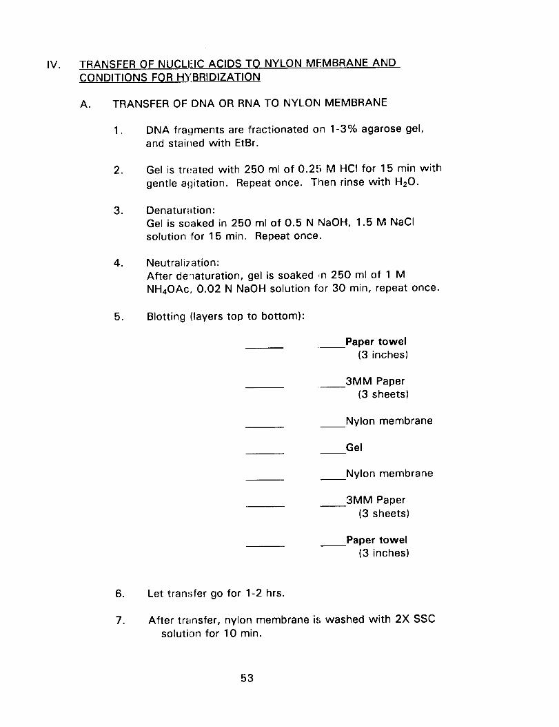
IV. TRANSFER OF NUCLI-IC ACIDS TO NYLON MEMBRANE AND
CONDITIONS FOR HYBRIDIZATION
TRANSFER OF DNA OR RNA TO NYLON MEMBRANE
°
.
.
.
A.
DNA fragments are fractionated on 1-3% agarose gel,
and stair_ed with EtBr.
Gel is treated with 250 ml of 0.25 M HCI for 15 min with
gentle a(jitation. Repeat once. Then rinse with H20.
Denaturation:
Gel is soaked in 250 ml of 0.5 N NaOH, 1.5 M NaCI
solution for 15 min. Repeat once.
Neutrali_ation:
After denaturation, gel is soaked _n 250 ml of 1 M
NH4OAc, 0.02 N NaOH solution for 30 min, repeat once.
5. Blotting (layers top to bottom):
Paper towel
(3 inches)
3MM Paper
(3 sheets)
Nylon membrane
Gel
Nylon membrane
3MM Paper
(3 sheets)
Paper towel
(3 inches)
.
7.
Let tran:_fer go for 1-2 hrs.
After tr{_nsfer, nylon membrane is washed with 2X SSC
solution for 10 min.
53
. Place the membrane into the Stratalinker UV crosslinker
while the membrane is still damp, but not dripping wet.
. Use auto crosslink mode to UV cross-link nucleic acids
onto the membrane.
10. Wrap with aluminum foil and store in dry place.
Reference:
G.E. Smith, and M.D. Summers (1980). Thebidirectional transfer of DNA and RNA to nitrocellulose
or diazobenzyloxymethyl paper. Analytical
Biochemistry 109:123-129.
54

B. HYBRIDIZATION CONDITIONS
(A) Conditions of nucleic acid hybridization depend on thetype of probes being used:
• DNA fiagment probes prepared from nick-translation or
random priming method:6X SSC
50% Formamide
5X Denhardt's
0.1% SDS
100 pg/ml denatured calf lhymus DNA3,_P-labeled DNA (at least 2 x 10⁶ cpm/ml)
Incub_,te at 42oC overnight
, Probe.,; prepared from end-labeled oligomers:6X SSC
5X Denhardt's
C. 1% SDS
0.05% Na-pyrophosphate
End-labeled oligonucleotide
Hybricization temperature is 5-7oC below md (dissociation
temperature), which is estimated by the following
equation:
Td = 4X (G + C) + 2x (A + T)
(B) Washing Conditions:
1.Wa.._h filters at room temperature with 4 changes of
solution of 2X SSC and 0.1% SDS, 5 min each.
2. Wash filters at 42oC with 2 changes of 1X SSC and
0.1% SDS, 30 min each.
3. Blol dry and expose to X-ray film.
55

V. DNA SEQUENCING WITH T7 DNA POLYMERASE (SEQUENASE)
° Annealing mixture:
ssDNA(O.O5pg/pl) 5 pl
H20 3 pl
10X buffer 1 pl
primer(0.5 pmole/pl) 1 pl
total 10pl
Anneal by heating at 80oC for 2 min and cool slowly at 37oCfor 30 min.
. While cooling, label four tubes as G, A, T, and C and fill each
tube with 2.5 /zl of each termination mixture ddG, ddA, ddT,
and ddC, respectively.
. Dilute enough T7 DNA polymerase (Sequenase) (1:8) for all
templates in icy cold TE buffer.
. Labeling reaction:
following:0.1 MDTT
lX labeling mixS3s or p32 dATP
diluted Sequenase
To annealed DNA mixture (step 1), add the
1 pl
2 pl
1 pl
2 pl
Mix and incubate at room temperature for 5-10 min.
. Transfer 3.5 pl of labeling reaction mix (step 4) into each
termination tube (step 2), mix and incubate at 37oC for 5 min.
o Stop the reaction by adding 5 pl of stop solution (0.03%
bromophenol blue; 0.03% xylene cyanol FF in 100%
formamide).
. Heat samples to 80oC for 2 min and immediately load into the
6% sequencing gel.
56

NOTE:(A)
(B)
For sequencing double-stranded plasmid DNA, please
follow this protocol
• Denaturation:
DNA 5 pl (1-2 pg)
2 N NaOH + 2rnM EDTA 2 pl
H20 15 pl
Total 22 pl
Mix and incubate at room temperature for 5 min.
. Neutralization:
Add 8 pl 1 M Tris-HCI (pH 4.5)
3 pl 3 M NaOAc (pH 5.6)
75 pl ETOH
Leave it at -80oC for 10 min, and spin down DNA.
• Dry down DNA sample and resuspend it in 7 pl of
water. Add 1 pl of primer and 2 pl of 5X buffer,
and incubate at 37oC for 15 min.
4. Then, continue from step 2 of previous section•
Sequencing of single stranded DNA templates prepared
by Asymmetric PCR amplification
0 Design amplification primers at least 200 base
pairs 5' to the site of sequencing primer.
° Carry out PCR amplification using 1:50 ratio of
amplification primers.
. After PCR amplification, add 10 pl of 3 M NaOAc
(pH 5.2) and 200 pl i.,,opropanol to each sample.
The samples are mixed and allowed to sit for 30
min at room temperature, then pelleted by
centrifuge for 30 rain at room temperature,washed once with 0.5 ml 70% ETOH and dried.THIS IS CRITICAL IN ORDER TO REMOVE EXCESS
•
AMOUNTS OF AMPLIFICATION PRIMERS.
Resuspend the DNA in 40 pl of TE buffer and be
ready for sequencing.
57
(C) Sequencing of double stranded DNA templates prepared
by Symmetric PCR amplification
• After PCR amplification, clean up products by
GENE CLEAN kit if you have a single DNA band on
the gel. Otherwise, run an agarose gel and slice
out the band you are interested in and purify it
through GENE CLEAN kit.
. Boil the DNA sample with primer in the lX
sequencing buffer for 5 min, then leave the tube in
either liquid nitrogen or ETOH-dry ice bath for 3min.
o Keep the frozen tube in the -20oC heat block insertand leave it there until the insert returns to the
room temperature.
, The tube is now ready for sequencing reaction
using the Sequenase kit.
58

(D) Reagent._ of Sequenase kit:
• 5X Sequenase buffer:
200 mM Tris-HCI (pH 7.5)
100 mM MgCI2
250 mM NaCI
. 5X Labeling Mix:
7.5 #M dGTP
7.5 #M dCTP
7.5 #M dTTP
3. Termination Mix:
ddG ddA ddT ddC
dGTP 80#M 80pM 80#M 80#M
dATP 80#M 80pM 80#M 80#M
dTTP 80#M 80pM 80#M 80pM
dCTP 80#M 80pM 80#M 80 #M
ddGTP
ddATP
ddTTP
ddCTP
8 #M
8 #M
8 #M
8 pM
NaCI 50mM 50mM 50mM 50mM
. Stop Solution:95% Formamide
20 mM EDTA
0.05% Brompheflol Blue
0.05% Xylene Cyanol FF
= 6%
42 g10 ml
0.3 ml
25 pl-- ml
1O0 ml
Sequencing Gel:
20 ml 30% Acrylamide Solution
(29:1 Acrylamide:Bis-Acrylamide)
Urea (final concentration is 7 M)
IOX TBE buffer (0.89 M Tris-HCI,
0.89 M Boric Acid, 2 mM EDTA,
pH 8.3)10% Ammonium PersulfateTEMED
H20final volume
59

(E) Conditions of running Gel (used with 0.4 mm wedge spacers):
o
2.
.
.
Pre-run sequencing gel at 1200 volts (constant voltage)for 1/2 to 1 hour.
Run samples at 1450 volts for 2 hours and 45 rain for
the first loading. The xylene cyano FF dye should be 27cm down from the wells.
Run the second loading for another 1 hour and 45 min
and stop the gel. You should be able to read the veryfirst base of the sequence.
In order to resolve 600 to 800 bases from the
sequencing reactions using M13 single stranded DNA as
templates, please use the following modifications toobtain the best results:
(a) Run a 6% sequencing gel at 1200 volts (constant
voltage) for 16 to 18 hours. Be sure gel is not
leaking!
(b) Run an 8% sequencing gel at 1200 volts for 8
hours, 4 hours per loading.
6O

VI. POLYMERASE CHAIN REACTION ASSAY CONDITIONS
1. Recommendec working dilutions:
Note: Use .,;terile, siliconized microfuge tubes.
Ao dNTPs Mix: Prepare a mix of dNTPs, 1.25 mM (in
each dNTP) final concentration.
Example:
125 /Jl
125 #1
125 #1
125 /11
500 pl
1000/_1
dATP 10 mM
dCTP 10 mM
dGTP 10 mM
dTTP 10 mM
Double-distilled, sterile water
dNTPs mix, 1.25 mM (in each dNTP) final
concentration
g. Control template: Prepare lO-fold serial dilutions of the
cont'ol template in 10 mM Tris-HCI pH 8.0, 1 mM EDTA
pH 8.0, 10 mM NaCI. (Do at least a 10-1 dilution).
C, Dep{.,nding on the sample DNA preparation procedure,
the ._uggested concentration of Mg+ + may not be
optimal for an efficient amplification. It may be advisable
to initially conduct a Mg+ + titration experiment in the
presence of an excess amount of _ Polymerase (i.e., 4
unit,,, of enzyme/sample). Once the optimum Mg+ +
concentration for a given DNA sample is determined, it is
recommended to carry out a _ Polymerase titration in
order to optimize the amount of enzyme required for a
max mum amplification efficiency.
Note: Brielly (about 2 seconds) vortex, then spin down (quick
spin with the tabletop microcentrifuge) the enzyme
before pipetting. Use extreme caution and proceed
slowly with the pipetting. The enzyme storage buffer
contains 50% glycerol and errors can be easily
introduced by hasty pipetting. If possible, use a positive
disp acement pipetting device.
61

2. Reaction Mix (per assay):
.
Note: Use sterile, siliconized microfuge tubes. This is the
standard protocol for the control template. Overlay the
samples (100 pl in 0.5 capped polypropylene tubes) with
100 pl of mineral oil (such as Sigma Cat. No. 400-5 or
M-3516) to prevent evaporation. The oil layer will not
interfere when withdrawing aliquots from the sample for
analysis. If the whole sample (100 pl) needs to be
recovered, extract the sample with 100 pl of chloroform
(high purity grade). The aqueous phase, containing thesample, will form a micelle near the meniscus. It will
then be easier to collect the sample by withdrawing itwith an Eppendorf pipette. Larger master mixes can be
prepared and aliquoted before adding the template and
the _ Polymerase. If you suspect that your template is
contaminated with proteases (as may be the case with
genomic DNA), add the _ Polymerase after the initial
denaturation step. The high temperature incubation
should inactivate proteases and prevent degradation ofthe Taa Polymerase.
Experimental Protocol:
Note: Performance of the PCR technique with the GeneAmpTM
DNA Amplification Reagent Kit, including Taa
Polymerase, can be automated with the PERKIN ELMER
CETUS DNA Thermal Cycler. The instrument enhances
the user's ability to control and optimize the PCR
technique to achieve maximum amplification efficiency.
Operating instructions and protocol recommendations for
use with the DNA Thermal Cycler are contained in the
Operator Manual. The following manual procedure is
recommended for those using heat blocks or water
baths. Use heat blocks or water baths (one each)
adjusted to the following temperatures: 37oC, 72oC, and
94oC. Initial template denaturation step: 1 rain. 30 sec.
at 94oC. Afterwards, a typical cycle profile will be:
2 minutes at 37oC (annealing)3 minutes at 72oC (extension)
1 minute at 94oC (denaturation)
Repeat for a total of 24 additional cycles. At the end of
the 25th cycle, OMIT the heat denaturation step andextend the extension step by an additional 7 minutes.
62

Foliowing the termination of the assay, let the samplescome back down to room temperature. The samples can
be kept at +4oC overnight, pending further analysis.
Note: A. The size of the target sequence in your sample DNA
will directly impact the minimum time required for
proper extension (72oC incubation step). An
optimization of the temperature cycling profile should
be performed for each template, in order to obtain
rnaximum amplification efficiency.
a. Be aware that there is a significant lag time (30seconds to 1 minute) between the time tubes are
transferred from one temperature to another and the
time the samples actually reach the new set
temperature. The lag time will be a function of the
type of heat source and tubes used, the sample
volume and the temperature differential between
incubation steps. Adjust the length of the incubation
steps to compensate for this lag time. (Microfugetubes from Robbins Scientific of Mountain View, CA,
(,at. No. 1048, appear to provide the most satisfactory
performance.)
REFERENCES:
• Saiki, R.K., S. Scharf, F. Faloona, K.B. Mullis, G.T. Horn, H.A.
Erlich, and N. Arnheim (1985) Enzymatic amplification of/3-
globin genomic sequences and restriction site analysis for
diagnosis of sickle cell anemia. Science 230:1250-1354.
. Scharf, S J., G.T. Horn, and H.A. Erlich (1986) Direct cloning
and sequence analysis of enzymatically amplified genomic
sequences. Science 233:1076-1078.
1 Chien, A., D.B. Edgar, and J.M. Trela (1976) Deoxyribonucleic
Acid Polymerase from the extreme thermophile Thermus
aauaticus. J. BacterioL 127(3):1550-1557.
63

VII. PREPARATION OF SINGLE-STRANDED CDNA SYSNTHESIS FOR PCR
Synthesis of 1st strand cDNA:
- Add 10pl poly(A) +- RNA and 2 pg oligo(dT)12_18
- Incubate at 65oC for 10 min, 37oC for 5 min and on icefor 5 min.
- Add in order: 6pl 5X RT buffer
2 pl 600 mM/3-ME
3pl IOXdXTP30 U RNasin
20 U AMV Reverse transcriptase
- Add H20 to a final volume of 30 pl
- Incubate at 37oC for 1 hour, then on ice for 5 rain.
- Do ETOH precipitation as usual, ie, add 1/10 vol. of 3 M
NaOAc (pH 5.6) and 2.5 vol. of ETOH to the tube and keep itin -80oC for 15 rain.
- Spin in microfuge for 15 min, dry the pellet and resuspend it
in 100 pl sterile H20
- Aliquot 1 pl for PCR amplifications
VIII.
,
.
.
4.
.
6.
7.
8.
9.
CLONING OF DNA FROM PCR AMPLIFICATION
After PCR amplifications, run a 1.2% agarose gel to examine theproducts. If there is only one band with the expected size DNA, then
transfer whole reaction mixture to a clean 1.5 ml eppendorf tube and
proceed to step 2. If there are multiple bands on the gel, then run a
preparative gel, slice out the fragment you are interested in, and
continue with the following:
Add 3 vol. of Nal solution (from GENECLEAN kit) and 30 pl of
glassmilk (from GENECLEAN kit) to the tube, mix well and keep it on icefor 10 min.
Spin in microfuge for 30 seconds. Discard the supernatant.
Add 400 pl of NEWWASH solution to the tube and resuspend it well by
vortexing.
Quick spin in the microfuge and decant the supernatant.
Repeat steps 4 and 5 twice.
Add 50 pl of H20 to the tube and incubate at 50oC for 5 min.
Spin in the microfuge for 1 min and save the supernatant.
Aliquot 10 pl of DNA from step 8, and add 13 pl H20, 3 pl of IOX
Kinase buffer, 3 pl of 10 mM ATP (pH = 7.0), and 1 pl of T4 kinase
(10 uints/pl ) to a final volume of 30 pl . Incubate at 37oC for 1 hour.
64
Add 3/A of :3 M NaOAc (pH = 5.6) and 75 pl of ETOH to precipitateDNA.
Resuspend DNA in 11 pl of H20, and set up the following for filling in
and ligations
3NA (in H20) 1 1 /11
I Ox ligase buffer 2/A:<lenow (2 units/pl ) 1 /A
JNTPs (from PCR) 2/A
12.
Incubate at 1 5oC for 1 hour. Then, add 1 /JI of blunt-end vector DNA
(0.1 /Jg), 2/.,I of 10 mM ATP (pH =7.0) and 1 /JI of T4 ligase
(1 unit//A) to the same tube and continue incubation overnight.
Carry out tra ]sformation as usual.
65
STRATEGIES FOR CLONING AND CHARACTERIZING cDNA
I..Introduction
(i). Difference_ between cDNA and genomic genes
Complementary DNA (cDNA) is synthesized in vitro from mature
mRNA by reverse transcription. Hence, the sequence of a cDNA is
complementary to that of its corresponding mRNA. In other words, the
cDNA sequence of an mRNA contains only sequence of the 5' untranslated
region, the translated region, and the 3' untranslated regions of the mRNAmolecule.
A genomic gene contains the 5' control region, the transcribed
region, and 3' flanking regions of a gene. In the transcribed region there areexons and introns. Therefore, the main difference between a cDNA
sequence and its corresponding genomic gene is that the cDNA sequence
contains neither introns nor the 5' and 3' flanking regions of the gene.
(ii). Purooses of cloning cDNA and genomic genes
(a). A cDNA can be used for the following studies:
-serving as a probe for the isolation of a genomic gene
-serving as a probe for studying the expression of a gene
-studying the primary sequence of a protein
-for large scale production of biosynthetic proteins in microorganisms
(b). A genomic gene is routinely used in the following studies:
-studying the structure and evolution of a gene
-elucidating the regulation of expression of a gene at the molecularlevel
-for gene transfer studies
II. Messenger RNA Population in Eukaryotic Cells
(i). There are numerous species of mRNA molecules present in any
eukaryotic cell. Some of these mRNA species are present in high
abundance, while others are present in very low frequency. For instance:
66
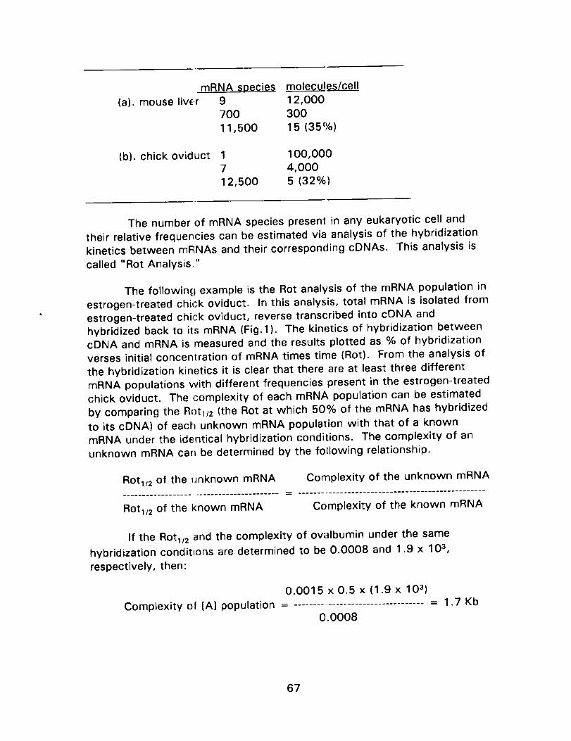
(a). mouse livc,r
(b). chick oviduct
mRNA species molecules/cell9 12,000
700 300
11,500 15 (35%)
1 100,000
7 4,000
12,500 5 (32%)
The number of mRNA species present in any eukaryotic cell and
their relative frequencies can be estimated via analysis of the hybridization
kinetics between mF_NAs and their corresponding cDNAs. This analysis is
called "Rot Analysis"
The following example is the Rot analysis of the mRNA population in
estrogen-treated chick oviduct. In this analysis, total mRNA is isolated from
estrogen-treated chick oviduct, reverse transcribed into cDNA and
hybridized back to its mRNA (Fig.l). The kinetics of hybridization between
cDNA and mRNA is measured and the results plotted as % of hybridization
verses initial concentration of mRNA times time (Rot). From the analysis of
the hybridization kinetics it is clear that there are at least three different
mRNA populations with different frequencies present in the estrogen-treated
chick oviduct. The complexity of each mRNA population can be estimated
by comparing the Rot1/2 (the Rot at which 50% of the mRNA has hybridized
to its cDNA) of each unknown mRNA population with that of a known
mRNA under the identical hybridization conditions. The complexity of an
unknown mRNA ca[_ be determined by the following relationship.
Rot1/2 of the unknown mRNA Complexity of the unknown mRNA
Rot1/2 of the known mRNA Complexity of the known mRNA
If the Rot_ 2 and the complexity of ovalbumin under the same
hybridization conditions are determined to be 0.0008 and 1.9 x 10³ ,
respectively, then:
0.0015 x 0.5 x (1.9 x 103 )
Complexity of [A] population .................................... = 1.7 Kb0.0008
67

' First l Seconcl
comoonent I component50% at 15% at
Rot_ 00015 Rot_/..0.04
I Finalcomoonem
35% atRd!,_.30
751
' ,} -Y7
eOl_
-: ?.r.
25
/
10-'_ 10 -s 10 -_' 10 -I 1 10 10 2
Rot
Hybridization between excew mlINA and cDNA idenlifies
several components in oviduct cells, each characterized by the
Rot,,_ of reaction.
Fig.l
68

0.04 x 0.15 x (1.9 x 103 )
Complexity of [B] population ................................... 14 Kb0.0008
30 x 0.35 x (1.9 x 103)
Complexity of [C] population ................................ 25000 Kb0.0008
If the average size of the mRNA in any population is about 2 Kb, then
there are 7 (14 Kb/2 Kb) different mRNA species in class [B] population, and
12500 (25000 Kb/2 Kb) .:lifferent mRNA species in class [C] population.
The average number of molecules of each mRNA per cell is called
abundance or representalion. It can be calculated quite simply if the total
mass of RNA in a cell is known, since for each component, total mass =
abundance x complexity, so that:
gm of mRNA in cell x fraction in component x (6 x 10²³ )Abundance ............................................................................
Complexity of component in daltons
In the example above, tht_,re are 0.275 pg mRNA per cell. This corresponds
to 100,000 copies of the first component mRNA, 4,000 copies of each of 7-
8 mRNAs in the second component, and about 5 copies of the 12,500
mRNAs in the third component.
(ii). cDNA library: a collection of cDNA clones that gives a fair
representation of all mRNA sequences present in a cell. In constructing a
cDNA library, effort is made to prepare sufficient amount of cDNA
molecules to will give a fi]ir representation of all the mRNA species.
The following equation is used to estimate the minimum number of
cDNA clones required for a complete cDNA library
In (1 -P)
N _ .................
h_ (1-1/n)
Where P is the probability, n is the fraction of the mRNA species under
consideration and N is tht,_ minimum number of the cDNA clones required in
the library. For practical consideration, P is usually 99%. Based on this
consideration, at least 200,000 recombinant cDNA clones are required to
cover all of the mRNA species present in a eukaryotic cell.
69

III. General Steps of Cloning cDNA Molecules
There are four general steps involved in cloning cDNA molecules:
(i) preparation of ds-cDNA molecules, (ii) construction of cDNA-vector
chimera, (iii) amplification of cDNA-vector chimera, and (iv) screening and
characterization. Depending on the frequency of mRNA under consideration
and the availability of probes for detecting the desired cDNA clone, the
actual strategy for constructing a library will vary. In this section I will
attempt to discuss all these issues.
(1). Preparation of ds-cDNA molecules for cloning
(a). Preparation of glassware and reagents for RNA extraction:
All glassware used in RNA extraction should be washed with
detergent and baked at 150oC for at least 6 hr. All plasticware can be
treated with 0.1% diethylpyrocarbonate (DEPC) or 10% H202. Reagents
that do not react with DEPC can be made RNase free by treatment with
DEPC (made 0.1% final concentration) and followed by autoclaving to
remove the excess amount of DEPC. RNase free water can be prepared bythe same method.
DEPC cannot be used as an RNase inhibitor for those solutions
whose active components are reactive to DEPC. In these cases, the
reagents are prepared in RNase free water.
(b). Preparation of total and poly(A)+-RNA:
Complete control of RNase activity during the course of RNA
extraction is the key to the successful isolation of undegraded RNA from
any source. In this regard, vanadyl ribonucleoside complex (VRC) has beenshown to be an efficient RNase inhibitor. Therefore, VRC is routinely
incorporated in the phenol-chloroform extraction method. Other potent
RNase inhibitors are guanidine thiocyanate and guanidine hydrochloride
because these two compounds are strong denaturation agents. Methods
have also been developed for RNA extraction by the use of guanidine
thiocyanate and guanidine hydrochloride buffer. In both methods, the ratio
of tissue to extraction is very important. For the liver tissue, 1-2 g of tissue
is routinely homogenized in 10 ml of the extraction buffer.
Another important factor leading to the success of RNA extraction is
deproteinization. This is commonly achieved by repeat extraction of the
tissue homogenate with phenol, phenol-chloroform and chloroform,
70

respectively. The RNA is recovered by precipitation with 2.5 volumes of
ice-cold ethyl alcohol.
There are several different methods developed for extraction of
undegraded RNA from different types of tissues based on the above
consideration. Detailed protocols for preparation of undegraded RNA atmini and maxi scales will be discussed in lectures.
Poly(A)÷-RNA is isolated from total RNA by affinity column
chromatography on oligo-(dT) cellulose. For routine reverse transcription
purposes, RNA isolated by one pass through an oligo-(dT) column is
required. The detailed protocols for RNA extraction and poly(A)+-RNA
isolation are described elsewhere in this publication.
(c). Synthesis of 1st and 2nd cDNA:
The first strand cDNA can be synthesized in vitro by reverse
transcription of poly(A)+-RNA, using oligo-(dT) as a primer and catalyzed by
reverse transcriptase isolated from avian myolocytomatosis virus. Generally
speaking, successful cDNA synthesis depends primarily upon total control of
RNase activity during the reaction. To achieve this goal, a potent RNase
inhibitor, RNasin, is routinely used. Since ethanol is a potent inhibitor for
reverse transcriptase, it should be removed from the RNA samples
completely. The standard conditions for the synthesis of the first strandcDNA is summarized below:
Tris-HCl(pH 8.3) 50 mM
MgCI2 10 mM
/3-mercaptoethanol 40 mMdXTP-dCTP 1.25 mM
dCTP 0.5 mM (a small amount of
RNasin
Reverse transcriptase
Poly(A) +-RNA
_-32[P]-dCTP is included in the
reaction in order to estimate
amount of cDNA synthesized)3O U
50 U
1 ug
Incubate at 42oC for 30 min.
In addition to the integrity and the secondary structure of mRNA, the
concentrations of Mg =' ion, reverse transcriptase, and dXTP will affect the
length as well as the yield of cDNA synthesized in vitro. Therefore, in order
to increase the length and the yield of cDNA, it is advisable to vary these
conditions sequentially in the course of cDNA synthesis.
71
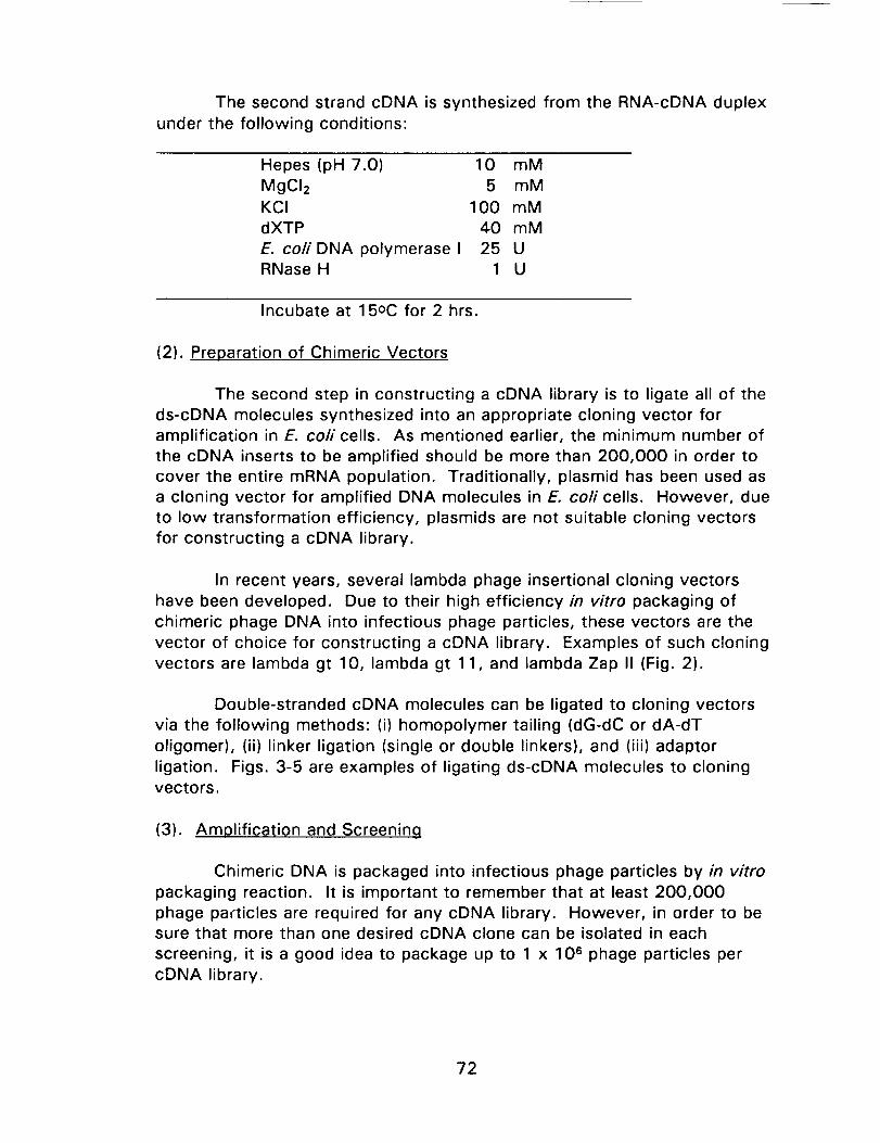
The second strand cDNA is synthesized from the RNA-cDNA duplexunder the following conditions:
Hepes (pH 7.0) 10 mMMgCI2 5 mMKCI 100 mMdXTP 40 mME. coil DNA polymerase I 25 URNase H 1 U
Incubate at 15oC for 2 hrs.
(2). Preparation of Chimeric Vectors
The second step in constructing a cDNA library is to ligate all of the
ds-cDNA molecules synthesized into an appropriate cloning vector for
amplification in E. coil cells. As mentioned earlier, the minimum number of
the cDNA inserts to be amplified should be more than 200,000 in order to
cover the entire mRNA population. Traditionally, plasmid has been used as
a cloning vector for amplified DNA molecules in E. coil cells. However, due
to low transformation efficiency, plasmids are not suitable cloning vectors
for constructing a cDNA library.
In recent years, several lambda phage insertional cloning vectors
have been developed. Due to their high efficiency in vitro packaging of
chimeric phage DNA into infectious phage particles, these vectors are the
vector of choice for constructing a cDNA library. Examples of such cloning
vectors are lambda gt 10, lambda gt 11, and lambda Zap II (Fig. 2).
Double-stranded cDNA molecules can be ligated to cloning vectors
via the following methods: (i) homopolymer tailing (dG-dC or dA-dT
oligomer), (ii) linker ligation (single or double linkers), and (iii) adaptor
ligation. Figs. 3-5 are examples of ligating ds-cDNA molecules to cloningvectors.
(3). Amplification and Screening
Chimeric DNA is packaged into infectious phage particles by in vitro
packaging reaction. It is important to remember that at least 200,000
phage particles are required for any cDNA library. However, in order to besure that more than one desired cDNA clone can be isolated in each
screening, it is a good idea to package up to 1 x 10⁶ phage particles per
cDNA library.
72
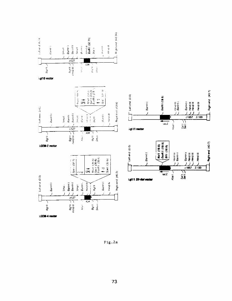
Z
kOtlO vector
0527
_--q ::
: /J
_.GEM-2 veclor
5E
I
_,_ _ __ _ _
/ /
o
E
kGEM-.,4
z_- _ _ -=T_ _: -= _
_ "'_ _s_ _ _,
o
- E
..4
v
-- --r- T ---- -- --
_ac Z
X_tll W
o
Fig.2a
73

I
IT_'rmln.iiof [nIIlalOf
clS_-
I. ConsU"u_ DNA Ubrary.
2. lso_te positive clone.
Clon¢_ DNA Insert
4--
f
J p_I- I cl8_'_
T_nllln]lor [nl[_ltor
co___.s
r
3. Excite _ pBlueK'ril_t' pl','mid
conUU_nt _.lae cloned DNA _ I_r
V co-_n with helpe_-plute.
T(wml_lK
pBlue_ript SK-
_.r3A
Flg.2b
74
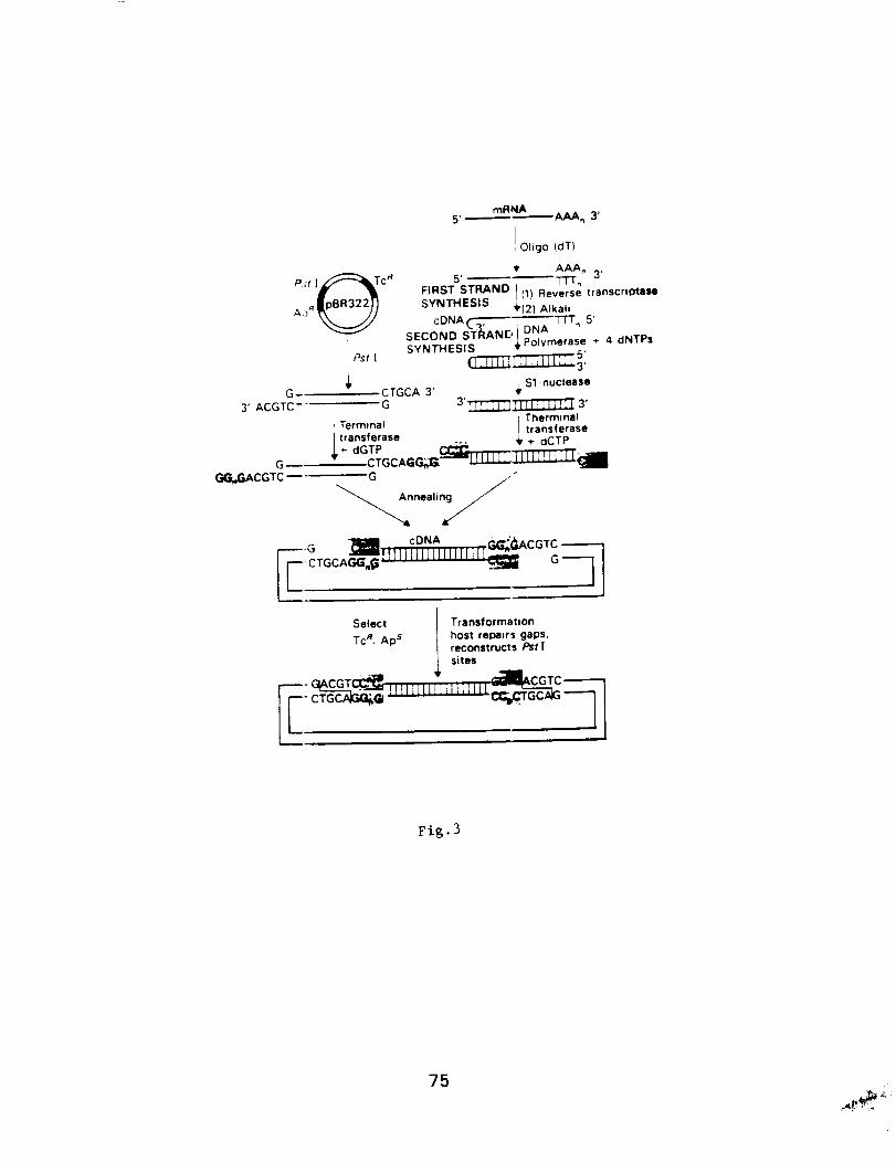
mRNA5' " AAA,_ 3'
Oligo (dT)AAA_
Pit I_cA 5' TTI'_ 3'
FIRST STRAND I(1) Reverse transcr,Dtase
A)n_,v.,___ll SYNTHESIS t(2) Alkali
cDNA(, DNA _114 5'SECONDST: ANDi] SYNTHESIS _ Polymerase _- 4 dNTPs
CTGCA 3' ; Sl-nuctease
G 3'_ ]1 ',[lii]I[I i III lII 3'
Terminal I Thermmal
I transferase ... _/transferase+dCTP
G
Annealing
G
3'ACGTC
G
C_.=,,_ACGTC --
Select Transformation
Tc R, ApS host fee)airs gaps,reconstructs ,°st [
sites
Fig. 3
75
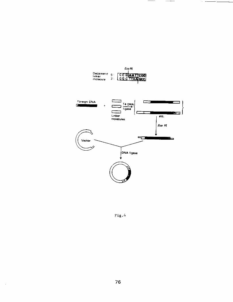
Oecamenclinkermolecule
Eco RI
Forefgn ONA
T4 DNA
ligase
Linker
molecules
r_
A ligase
0
etc.
Eco RI
Fig .4
76
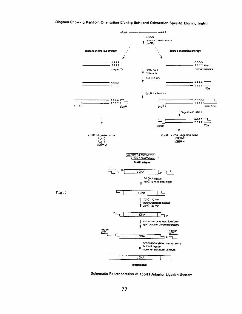
Diagram Showir, g Random Orientation Cloning (left) and Orientation Specific Cloning (right)
mRNA
,/
randomonem._ s_teW
/_AAA
rrTr
e.qo(aT_
• AAAA
TTTT
EcoQ
TTTT
EcoR
EcoR I ingested arms
_gtl0kgt_ I
kGEM-2
AAAA
I primer, ,everse lranscnotase
3NTPs
DNA DOIIRNase H
T4 ONA ool
I EcoF__adamo(s
T
EcoR I
detiMd nmatiea tm.lllr
AAAA
TTTTxDa
onmer-actaD_of
AAAA [_TTTT
Xba
AAAA_TTTT
×ha EcoF
i Digest w_tr_ Xba I.
tAAAA
TTTTXDa I
EcoR I I
EcoR I ÷ XDa I a_gesteO arms;LGEM-2
_.GEM-4
L._'crC CC T TGC TG TCGLGGCA_CAGCpP
E_R I _aitet
C:_]_p pJ oN, LPPC=
I T40NA _gase15=C. 6 hr to ov_rn_nt
Fig. 5
70_C, 10 n'_npownuc_ kmase37"C. 30 mm
I exvact',on oher, o_cNorotormspin column cnrornatogr_:)ny
veCtOr veCtO¢arm arm
deor',osonorylate_l vector armsT4 DNA Iigaseroom temoerature, 3 hours
Schematic Representation of EcoR I Adaptor Ligation System
77

Before a library is screened for any desired cDNA clone, it isroutinely amplified once by infecting every phage particle to E. coil cells. It
is important to note that every library can be amplified only once or the slow
growing recombinant phage particles will be eliminated in the subsequent
round of amplification.
Depending on the availability of probes, a cDNA clone can be
isolated from the cDNA library by any of the following three methods:
(i) Nucleic acid hybridization with a cDNA, genomic DNA, or
oligonucleotide probe.
(ii) Immunochemical screening with an antibody probe.
(iii) Screening based on the biological activity of the protein
encoded by the cDNA clone.
(Examples of each screening method were discussed in detail during thelectures. )
IV. Various Basic Strategies of Cloning cDNA Molecules
There are two basic factors that determine a particular strategy to be
adopted for cloning a cDNA sequence. These two factors are:
(i). The kind of probe available for the isolation of a cDNA clone of
interest from a cDNA library.
(ii). The relative abundance of an mRNA species of interest.
These two factors will dictate the actual cloning strategy that one should
follow in order to isolate the cDNA sequence of interest. In the following
section, several examples of cDNA cloning strategies will be discussed.
(1). Strategy of cloning a cDNA sequence when its mRNA is present under
a particular condition
In the event that you do not have a known nucleic acid or antibody
probe for the cDNA sequence that you intend to clone, you can still isolate
such a cDNA sequence if the corresponding mRNA can be induced by a
specific hormone, or if it is present in a specific cell type or a specific
developmental stage. There are several examples like this in the literature.
78

_oo I
E4O_2,_ _ Q r
20 ; ._
.Lo(j Rot
The effect of estra_ol tre.itment on mRNA sequencecomplexity. Jn the maletrout liver. [ )H]cDNA transcribed from
the tom/liver RNA of esu'adiol-ueat_ male fish was hylmdizedwith the total liver RNA of contsol and hormone-treated fish at68°C to the Rol values indicated. The extent of hybridizanonwas deterrmned by S_ nuclease digestion of the reactionmixture. O, total cDNA to total hver RNA of the esn, adiol-treated male fish; O, total cDNA to total liver RNA of thecontrol male fish.
a b
Northern blot hybridization of trout liver RNA witheDNA. "Iotal liver RNA of control and estradmi-Ueated
fish were electrophoresed on agarose gels in the lmmmm dmethylmercuric hydroxide and then u-ansferred to morozet.lukne filter. 32P-label|ed cDNA (sp.act.. 1 x 10_ c[_/_41
DNA) was prepared by reverse transcription using total fiverRNA of hormone-ureated male fish as a template. The
hybridization of cDNA to high frequency class hocmmm-specific mRNA was detected by exposure of the x-ray film tothe filter for 12 h at -70°C. (a) Twenty. micrograms of totalliver RNA of conu'ol male fish; (/7) 20 _.g o[ total liver RNA ofesu'adiol-ceated male fish.
Fig.6
79
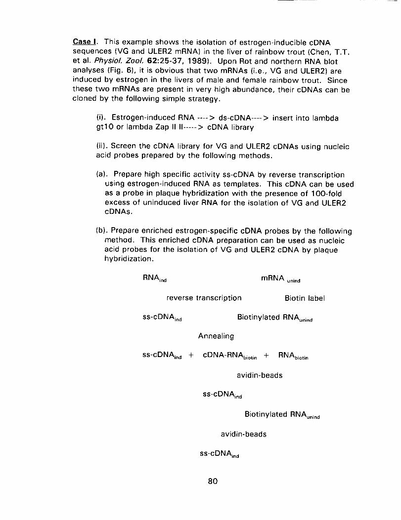
Case I. This example shows the isolation of estrogen-inducible cDNA
sequences (VG and ULER2 mRNA) in the liver of rainbow trout (Chen, T.T.
et al. Physiol. ZooL 62:25-37, 1989). Upon Rot and northern RNA blot
analyses (Fig. 6), it is obvious that two mRNAs (i.e., VG and ULER2) are
induced by estrogen in the livers of male and female rainbow trout. Since
these two mRNAs are present in very high abundance, their cDNAs can be
cloned by the following simple strategy.
(i). Estrogen-induced RNA .... > ds-cDNA .... > insert into lambda
gtlO or lambda Zap II II ..... > cDNA library
(ii). Screen the cDNA library for VG and ULER2 cDNAs using nucleic
acid probes prepared by the following methods.
(a). Prepare high specific activity ss-cDNA by reverse transcription
using estrogen-induced RNA as templates. This cDNA can be used
as a probe in plaque hybridization with the presence of l O0-foldexcess of uninduced liver RNA for the isolation of VG and ULER2cDNAs.
(b). Prepare enriched estrogen-specific cDNA probes by the following
method. This enriched cDNA preparation can be used as nucleic
acid probes for the isolation of VG and ULER2 cDNA by plaque
hybridization.
RNAin d mRNA unind
reverse transcription Biotin label
Ss-cDNAin d Biotinylated RNAunin d
Annealing
Ss-cDNAin d + cDNA-RNAbiotin + RNAbiotin
avidin-beads
Ss-cDNAin d
Biotinylated RNAunin d
avidin-beads
Ss-cDNAin d
8O

The above ss-cDNA is highly enriched with estrogen-responsive
cDNA sequence, and hence can be used as a probe for the isolation of
estrogen-induced cDNA sequences after it is radio-labelled by kinasereaction. Alternatively, this ss-cDNA can be used as templates for the
construction of a cDNA library by strategies to be discussed in the next
section.
Case II. If the mRNA in Case I is present in 1race quantity, the following
strategy can be followed.In this case, the enriched estrogen-responsive cDNA can be amplified
by PCR and then cloned into an appropriate cloning vector, e.g., lambda
Zap I1. The cloning strategy is described below:
............................ TTT-[ T 5'
Terminal trarlsferase to add "Cs"
CCC CC ........................... "1"-[TTT5'
use oligo(dG)-R1 and oligo(dT)-R1 as
primers in PCR to amplify the entire cDNA
population
R 1-CCCCC .......................... TTTTT- R 1
R1 -GGGGG ......................... AAAAA-R1
Methylation,
Digestion with restriction enzyme EcoR1,
Pass through Sephacryl 300 column
Ligate to lambda gtlO or lambda Zap II
in vitro packaging and amplification inE. coil cells
A PARTIAL cDNA LIBRARY
Screen the library with the enriched
estrogen-responsive cDNA as a probe
CLONES .......... ready for further characterization
81

Note: These two strategies are very useful in cloning cDNAsequences whose corresponding mRNAs are present under one condition
and absent in another condition. Examples are tissue specific mRNA,
developmental stage specific mRNA, and hormone or other agent induciblemRNA.
2. Strategy for cloning a cDNA sequence when portions of the
corresponding peptide sequence are known
(i). If the amino acid sequences of several portions of a polypeptide
are known, their corresponding nucleotide sequences can be derived by
referring to the genetic codes. Synthetic oligonucleotides can be made from
this information and used as probes for the isolation of the correspondingcDNA.
example:
peptide:Nucleotide
Cys Ilu Met Ala Glu Gly His Arg Asp CysUGU AUU ATG GCN GAA GGN CAU CGN GAU UGU
C C G CC A C C
A G
A mixed oligonucleotide of any length (17 to 27 mer) can be
synthesized based on the sequence shown above. One point worth notingis that the length of the oligomer should be long enough to preserve the
specificity. However, it can not be too long or the sequence combination
will be too high, and consequently the concentration of the correct oligomer
will be too low. More details about the design and use of the oligomer werediscussed in lecture.
(ii). If several oligonucleotides can be derived from different portions
of the polypeptide, these oligonucleotides can be used as primers for direct
PCR amplification of a portion of the cDNA sequence. After
characterization, the amplified cDNA fragment can be used as a probe for
the isolation of the full-length cDNA from a cDNA library. The strategy ofthe PCR amplification is described below:
N ............................................................... polypeptide
P1 P2 P3
amino acid sequence
oligonucleotide
82

Strategy of PCRampl fication:
Poly (A) +-RNA
reverse transcription
.......................................... cDNA
P1 and P3 as primersPCRamplification
Blunt end the amplified DNA moleculesClone into plasmid or M13Isolate positive clones by hybridization with P2
Positive Clones
confirm the result by nucleotide sequencedetermination
Clones are ready to serve as a probe
fo isolation of the desired (;DNA clone.
(iii). Assume you have some amino acid sequence information on the
cDNA that you are in_:erested in, but the amount of tissue that you can use
for RNA extraction is very limited. Obviously you can not prepare a
conventional cDNA library for the isolation of the desired cDNA clone. In
this case, the followit_g strategy can be tried. This is called a RACE method
to prepare a cDNA library. The strategy is outlined below:
N .................................................... polypeptide
...................... amino acid sequence
R1 ...................... R1 oligonucleotide
Poly(A) + -RNA
reverse transcliption
............................................ TTTTT 5'
addition of pol_(G) by terminal transferase
83
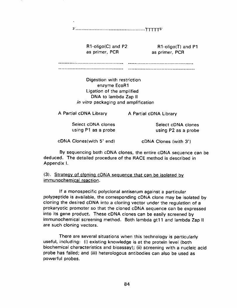
3'_........................................... TTTTTs'
Rl-oligo(C) and P2
as primer, PCRRl-oligo(T) and P1
as primer, PCR
Digestion with restriction
enzyme EcoR1
Ligation of the amplified
DNA to lambda Zap II
in vitro packaging and amplification
A Partial cDNA Library A Partial cDNA Library
Select cDNA clones
using P1 as a probe
Select cDNA clones
using P2 as a probe
cDNA Clones(with 5' end) cDNA Clones (with 3')
By sequencing both cDNA clones, the entire cDNA sequence can be
deduced. The detailed procedure of the RACE method is described in
Appendix I.
(3). Strategy of cloning cDNA sequence that can be isolated byimmunochemical reaction.
If a monospecific polyclonal antiserum against a particular
polypeptide is available, the corresponding cDNA clone may be isolated by
cloning the desired cDNA into a cloning vector under the regulation of a
prokaryotic promoter so that the cloned cDNA sequence can be expressed
into its gene product. These cDNA clones can be easily screened by
immunochemical screening method. Both lambda gt11 and lambda Zap II
are such cloning vectors.
There are several situations when this technology is particularlyuseful, including: (i) existing knowledge is at the protein level (both
biochemical characteristics and bioassay); (ii) screening with a nucleic acid
probe has failed; and (iii) heterologous antibodies can also be used as
powerful probes.
84

However, there are a few limitations about this approach.
(i). The protein must be purified or isolated
(ii). A large (1-2mg) amount of protein must be available
(iii). Some proteins are not suitable
(iv). Screening ('an be relatively tedious
(v). Success relies strongly on the nature of an unpredictable
immunological response
(vi). Immune response is slow (months).
These are:
More detailed information regarding this technique is provided in
Appendix II. If the biological activity of the gene product is known, a
bioassay of the gene product can also be developed for the isolation of the
corresponding cDNA sequence. Examples will be given in lecture to explain
such a screening strategy.
85

Appendix I: RACE
1. Prepare RNA using a protocol that yields high quality RNA. If micro scale
preparation of RNA from small tissues is required, the 4 hr prep (also calledacid phenol) or other easily scaled down methods are advisable. In small
scale preps, add 2/_g 5s E. coli ribosomal RNA (NOT yeast tRNA).
2. Dissolve the final RNA pellet in 10#1 dH20 if using a small scale prep. For
larger preps, only 10#g RNA is required, mRNA enrichment is not necessary
in this method, and in the micro scale preps it is also unadvisable sincesubstantial loss is possible.
. USE RNase FREE PRACTICES UNTIL NOTIFIED OTHERWISE
a. use gloves
b. all reagents should be made in DEPC treated dH20
c. pipet tips and all tubes used should be autoclaved before use
4. First strand reaction
a. Add:
10 #1 RNA
2 #1 oligo-dT12.18 (2 #g)
b. Heat to 65oC for10 min.; 37oC for 5 min.; then chill onice for 5 min.
c. Add in order:
6/_1 5X RT buffer
2 #1 600 mM/3-ME
3#1 10XdXTP
2 #1 e-P3=-dCTP30 U RNasin
50 U Reverase transcriptase
add water to a final volume of 30 #1.d. Incubate at 42oC 1 hr., then 52oC for 30 min.
5. Add 0.70/_1of 1XTE.
6. Heat the reaction to 99oC for 5 min.
7. Spin cDNA through a Saphacryl-300 column, and precipitate the cDNA
with 2.5 volumes of EtOH (add 5/_g 5S rRNA as the carrier). Incubate the
mixture at -80oC for one hour. Spin down the pp't in an Eppendorf
centrifuge at the top speed for 30 rain in the cold. Wash the pp't in 70%
EtOH, dry and resuspend in 12/_1 of water. Take one #1 for radioactivity
determination (in order to calculate the amount of cDNA made). Take
another #1 for size determination by electrophoresis on 1.5% agarose gels.
86

8. Tailing reactiona. Add:
10 #1cENA1 #14 mM dGTP4 /_1 5_( tailing buffer (supplied with the terminal transferase)
2 /_1 t_.rminal transferase (30-60U)
3 #1 CoCI2 (not required with some enzymes, supplied with
enzyme if required. Substitute: dH20 if not required)
b. Incubate the reaction at 37oC for 30 rain.
c. Heat the reaction mixture at 65oC for 5 min.
d. Precipitate the cDNA by adding 2.5 volumes of EtOH, collect the
pp't, wash in 70% EtOH, dry, and dissolve the cDNA in 20/_1
of water.
AT THIS POINT YOU NO LONGER NEED TO MAINTAIN AN RNase FREE
ENVIRONMENT
9. PCR
a. Add:
10
2
1
1
#1 1(iX TAQ polymerase buffer (supplied with the enzyme)
#1 each of the dNTP (usually at 10 mM stock conc.)
#1 primer 1 (1 /_g//_l)
/_1 primer 2 (1 /_g/#l)b. Add entire cDNA volume
c. Add enough JH20 so that the reaction volume is now 99.5 /_1
d. Heat at 95oC for 5 min.; cool to 72oC
e. Add 0.5/zl TAQ polymerase (2.5 U)f. Add mineral oil
g. Cycle 95oC 1 min.; 55oC 1 min.; 72oC 3 min. for 40 cycles
h. This is a higl _ stringency guideline, actual conditions may be
empirically determineci. Extend at 72oC for 15 min.
11. Remove the mineral oil
12. Digest PCR product with EcoR1
a. digest setup
89 /_1 P(,'R product
10 /_1 IOX EcoR1 buffer (supplied with enzyme)
1 #1 EcoR1 (10 U)b. incubate at 37oC for 1 hr, stop digesl with 5 /_1 .5 M EDTA and
heat to 65oC for 10 rr, in.
c. Run the PCR product digest over a spin column (Sephacryl-300)
87

14. Quantitate spin column effluent with spectrophotometry or fluorometry
15. Resuspend aliquote of the PCRproduct to 50 ng//_l
16. The ligation
a. If a low amount of cDNA is present add:
2.5 #1 DNA (the entire PCR product)
0.5 #1 10 mM ATP (store on ice <20 min. or at -20oC)
0.5/_1 IOX ligation buffer (store on ice)
0.5 M TRIS pH 8.0
70 mM MgCI2
1.0/_1 phage arms(1 #g) (store ONLY at -20oC)
0.5 #1 HIGH CONCENTRATION LIGASE (store ONLY at -20oC)
b. If a high amount of cDNA is present set up 2 reactions
A B
DNA 1 #1 (50 ng) 2.5 #1 (125 ng)10 mM ATP 0.5 0.5
IOX lig. buf. 0.5 0.5
arms 1.0 1 .O
dH20 1.5 0.0
HIGH
CONCENTRATION
LIGASE 0.5 0.5
c. Mix ligations GENTLY but sufficiently to homogenize
d. Spin 5 sec. in the microfuge
e. Ligate 4oC overnight
Comments about RACE
1. With RACE, only one area of nucleotide homology is required.
2. The area of homology can either be 3' within the gene (as in this
protocol) or 5', as would be obtained by N terminal amino acid sequencing.
3. If a 5' region is used, the poly A tail of mRNA is used rather than addinga poly G tail.
4. Both PCR primers MUST have restriction sites built onto them, so that
they will be clonable into the phage vector.
88
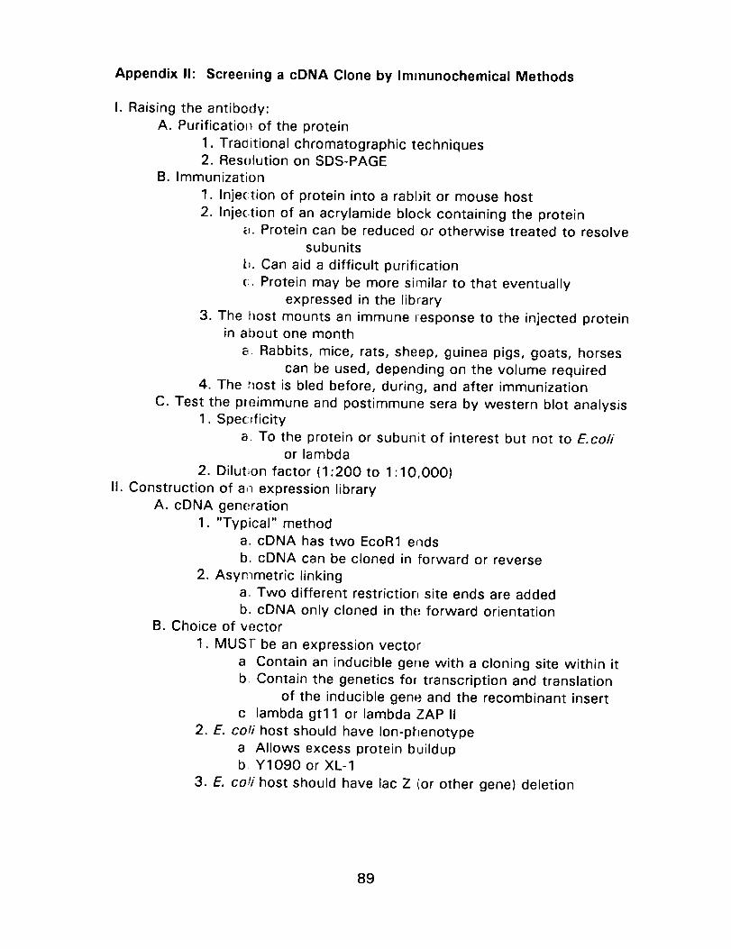
Appendix I1: Screening a cDNA Clone by Immunochemical Methods
I. Raising the antibody:
A. Purification of the protein
1. Traoitional chromatographic techniques2. Resolution on SDS-PAGE
B. Immunization
1. Injection of protein into a rabbit or mouse host
2. Inje(tion of an acrylamide block containing the proteinz_. Protein can be reduced or otherwise treated to resolve
subunits
b. Can aid a difficult purification
(. Protein may be more similar to that eventually
expressed in the library
3. The host mounts an immune response to the injected proteinin about one month
_. Rabbits, mice, rats, sheep, guinea pigs, goats, horses
can be used, depending on the volume required
4. The r_ost is bled before, during, and after immunization
C. Test the preimmune and postimmune sera by western blot analysis
1. Specificity
a. To the protein or subunit of interest but not to E.colior lambda
2. Dilution factor (1:200 to 1:10,000)
II. Construction of a,_ expression library
A. cDNA generation
1. "Typical" methoda. cDNA has two EcoR1 ends
b. cDNA can be cloned in forward or reverse
2. Asymmetric linkinga. Two different restriction site ends are added
b. cDNA only cloned in thE; forward orientationB. Choice of vector
1. MUST- be an expression vector
a. Contain an inducible gene with a cloning site within it
b, Contain the genetics for transcription and translation
of the inducible gene and the recombinant insert
c lambda gt11 or lambda ZAP II
2. E. coti host should have Ion-phenotype
a Allows excess protein buildupb Y1090 or XL-1
3. E. coti host should have lac Z (or other gene) deletion
89

II1. Basic Screening Procedures
A. Preparation of blots1. Grow infected bacteria 4 hrs. at 42oC
2. Soak NITROCELLULOSE filters in 10 mM
3. Overlay plates with filters
4. Grow 4 hrs to overnight at 37oC or room temperature
5. Expressed proteins adhere to nitrocellulose when filters are
lifted off the plates
B. Incubation with the primary antiserum
1. Reabsorb the primary antiserum with E. coil extract to render
specific to the antigen of interest2. Filters are first blocked with 1%BSA, 20% BCS, or milk
3. Primary antisera incubation is 30 min at room temperature
or overnight at 4oC
C. Incubation with the secondary antibody
1. Secondary antisera is goat anti-rabbit fused to alkaline
phosphatase or horseradish peroxidase
2. Filters are incubated with the secondary antibody (1-1000
dil.) for 30 to 60 min at room temperature
3. Wash the filters with blocking solution
D. Color development
1. Alkaline phosphatase or horseradish peroxidase activity isassayed for any phage plaque. The correctly expressed
fusion protein will have the rabbit primary antibody bound to
the nitrocellulose in a corresponding position.
90

Appendix II1: Amplification of the Lambda Zap-II Library
It is usually desirable to amplify libraries constructed in lambda
vectors in order to obtain a large quantity of high titer and stable stock.
However, more than one round of amplification is not recommended since
slow growing recombinant clones may be significantly reduced in the
process of amplification. In some cases, the cDNA library is screened
without prior amplification. The host cell strain used to amplify or plate
lambda Zap-II clones is E. coil XL-blue, which grows well in L-broth.
1. Preparation of Host Cells
E. coil XL-blue strain is used as host cells for the amplification or
plating out of the library for screening. The plating host cells should be
started from a single colony. Bacterial cells from a single colony are
inoculated to 100 ml of L broth supplemented with 0.2% maltose and 10
mM MgSO4, and grown overnight at 30oC under vigorous shaking. Cells are
collected by centrifugation at approximately 6,000 rpm and resuspended in
0.5 volumes in 10 mM MgSO4. These cells are called plating cells, which
are good for up to lwo weeks at 4oC.
2. Amplification
(a). Dilute plating ct;lls with 10 mM MgSO4 so that 600/_1 of the diluted
cells will give O.D.6oo = 0.5.
(b). Mix aliquots of the packaged lambda clones (about 50,000 recombinant
clones) with 600/_1 of the diluted plating cells in Falcon tubes.
(c). Incubate tubes containing phage and host cells for 15 rain at 37oC.
(d). Mix 8 ml of melted (48oC) top agar (NZCYM broth containing 0.7%
agarose) with each aliquot of infected bacteria and pour evenly onto the
150 mm NZCYM plate (NZCYM broth containing 1.5% agar).
(e). Incubate plates at 37oC for 5-8 hrs. Do not allow the plaques to get too
large.
(f). Flood each plate with 10 ml of SM buffer (containing 5.8 g of NaCI,
2.0 g of MgSO,, 50 ml of 1 M Tris-HCI (pH 7.5), and 5 ml of 2% gelatin).
Incubate the plates at 4oC overnight with gentle shaking or rocking.
(g). Recover the bacteriophage suspension from each plate and pool into asterile tube. Add chloroform to 5% and invert to mix.
91

(h). Remove cell debris by centrifugation for 5 min at 6,000 rpm.
(i). Collect the supernatant, pool and store in a glass or polypropylene
bottle. Add chloroform to 0.3% and store in aliquots at 4oC.
(j). Determine the titer of the library.
Appendix IV: EXTRACTION OF HIGH MOLECULAR WEIGHT DNA
(a). Resuspend 2 ml of red blood cell pellet in 5 ml 1X SSC.
(b). Add 5 ml of TNE buffer (100 mM Tris-HCI, pH 7.5; 100 mM NaCI; 10
mM EDTA; 1% sarkosyl), and mix gently by rotating the tube for 2-3 min tolyse the cells. (DO NOT SHAKE THE TUBE OR YOUR DNA WILL BE
SHEARED INTO PIECES). Add freshly prepared proteinase K to 100 #g/mlfinal concentration.
(c). Incubate the tube at 55oC for 2 hr. Then add 10 ml TNE buffer.
(d). Extract the sample, one time each, with equal volumes (20 ml) of
freshly saturated phenol, phenol-chloroform (1:1 v/v), and then chloroform-
isoamyl alcohol (24:1 v/v). The organic phase is separated by centrifugation
at 3,500 rpm for 10 rain. In each extraction, the aqueous phase is
transferred to a clean tube with a pipette whose entire tip is cut off in order
to avoid (i) shearing the DNA molecules and (ii) pulling the interphase intothe DNA solution.
(d). Transfer the aqueous phase into a dialysis tube and dialyze the aqueous
phase against 4 liters of TE buffer (10 mM Tris-HCI, pH 7.5, 1 mM EDTA)
for 24 hr. with several changes of the buffer.
(e). Estimate the DNA concentration in each sample by electrophoresis of
DNA samples on a 0.4% agarose gel (mini gel).
92

Molecular Approaches to the Analysis of
Population Polymorphisms and Enzyme Expression
Prepared by: Douglas Crawford, University of Chicago
and Simona Bartl, Hopkins Marine Station, Stanford Univ.
Contents:
RNA Isolation
Restriction Enzyme Digest
In Vitro-produced mRNA and cRNA
RNA gelNorthern Blot
Fragment Purification: Agarose
Random PrimingmRNA to cDNA
Southern Blot
Hybridizations: RNA or DNA
RNA Dot Blot
T4 DNA Polymera,,;eMedia for Bacteria
Preservation of Animal Tissue at Room Temperature
for DNA An,_lysesGeneclean: the Wonders of Glass and DNA
Boiling Minipreps for Plasmid DNA
94
96
97
98
98
99
100
101
102
103
104
105
106
107
108
109
93

RNA ISOLATION
Chaos Buffer for RNA isolation
4.5M
2%
50 mM
25 mM
0.1M
0.2%
Guanidinium thiocyanate
N-lauroylsarcosine (sarcosyl)EDTA
Tris-HCI, pH 7.5
/3-mercaptoethanol
For 100 mls:
53.2 g
2.0g10mlsofO.5 M
2.5 mlsof 1 M
700 #1
antifoam A (Sigma)
5.7 M CsCI cushion
FINAL VOLUME
5.7 M "Baked" CsCI
0.1 M EDTA
100 ml
95.8 g20 mls of 0.5 M
Use DEPC treated water and baked glassware. This solution, absolutely,
positively must be RNase free. RNase is everywhere[ Wear gloves and
use only baked glassware or virgin plastic. DEPC treat your water and
buffers (except Tris). Be very careful.
2
3
4
4A
4B
5
6
7
8
9
Weigh animal.
Remove organ (liver) and weigh. (One of the superior attributes of
cDNA is you reduce the gene complexity by choosing an organ that
expresses only a single locus of a multilocus enzyme.)
Homogenize tissue rapidly in "Chaos" buffer (9 mls).
Spin homogenant at 10 KG to remove insoluble material.
While homogenant is spinning:
Weigh out 1.8 g of CsCI (0.2g/ml) per sample.
In the ultra-centrifuge tube ("quick-seal") add 3.5 mls of 5.7 M CsCI
"cushion." This layer must be RNase free. You will centrifuge your
RNA through this layer and any contamination will cause significantloss.
Remove supernant, put into fresh tube, and add 1.8 g CsCI.
Carefully add homogenant on top of the CsCI cushion. This is most
readily accomplished by using a lOcc syringe and long needle. Place
needle/syringe into quick-seal tube, and add tissue homogenant to the
syringe. Homogenant will slowly trickle into Q-S tube, floating on topof the cushion.
Carefully balance matched pairs of centrifuge tube (+/-0.005 g).
Seal tubes, place matched tubes opposite of each other, and cap with
red aluminum tops.
Centrifuge 50,000 rpms, 5.5 hrs, 20oC.
94
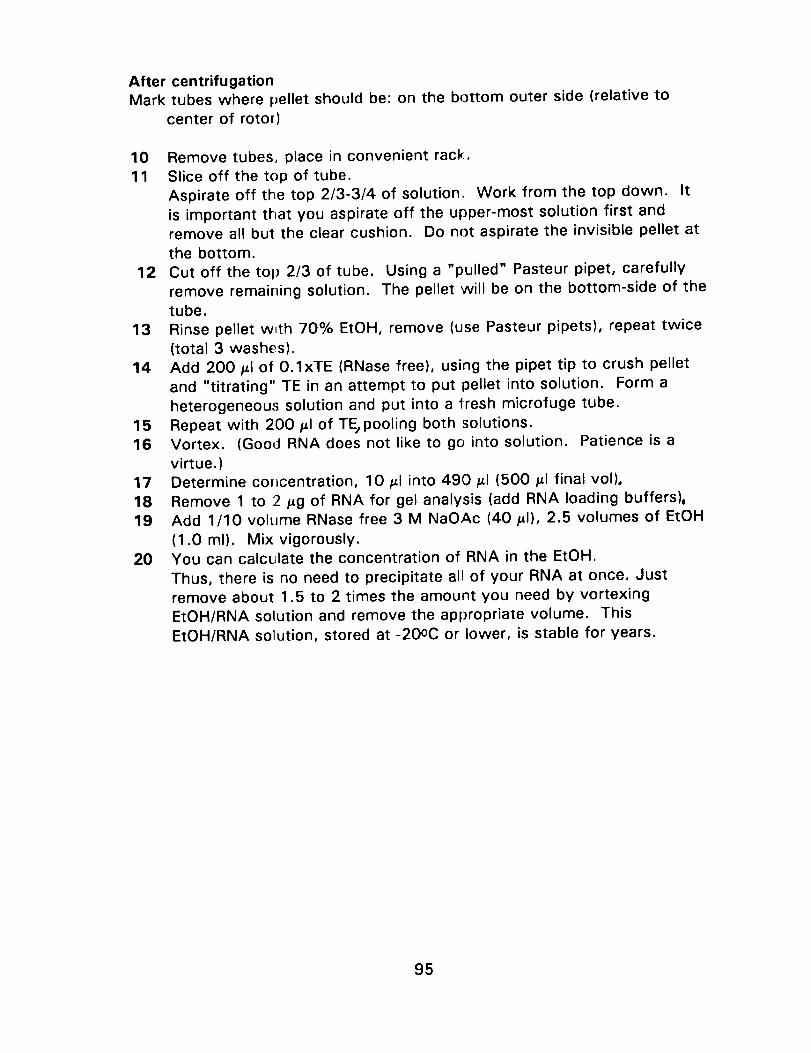
After centrifugationMark tubes where pellet should be: on the bottom outer side (relative to
center of rotor)
10 Remove tubes, place in convenient rack.
11 Slice off the top of tube.
Aspirate off the top 2/3-3/4 of solution. Work from the top down. It
is important that you aspirate off the upper-most solution first andremove all but the clear cushion. Do not aspirate the invisible pellet at
the bottom.
12 Cut off the top 2/3 of tube. Using a "pulled" Pasteur pipet, carefully
remove remaining solution. The pellet will be on the bottom-side of the
tube.
13 Rinse pellet with 70% EtOH, remove (use Pasteur pipets), repeat twice
(total 3 washes).
14 Add 200/_1 of 0.1xTE (RNase free), using the pipet tip to crush pellet
and "titrating" TE in an attempt to put pellet into solution. Form a
heterogeneous solution and put into a fresh microfuge tube.
15 Repeat with 200 #1 of TEj pooling both solutions.16 Vortex. (Good RNA does not like to go into solution. Patience is a
virtue.)17 Determine cm_centration, 10/_1 into 490/_1 (500/_1 final vol),
18 Remove 1 to 2/_g of RNA for gel analysis (add RNA loading buffers),
19 Add 1/10 volume RNase free 3 M NaOAc (40/_1), 2.5 volumes of EtOH
(1.0 ml). Mix vigorously.20 You can calculate the concentration of RNA in the EtOH.
Thus, there is no need to precipitate all of your RNA at once. Justremove about 1.5 to 2 times the amount you need by vortexing
EtOH/RNA solution and remove the appropriate volume. This
EtOH/RNA solution, stored at -20oC or lower, is stable for years.
95

While RNA is centrifugating,1 Digest pSP6LDHB with BamHI, so we can use this linearized DNA to
produce cRNA.
2 Pour RNA gel.
RESTRICTION ENZYME DIGEST
10g of pSP6LDHB
5 #1 Restriction buffer (medium)
34 #1 dH20
1#1 Bam HI37oC for 2+ hrs.
Normal DNA digest with restriction enzymes is in a total volume of 50 #1
(microliters, 10-6 liters, or X). You can do the digest in a smaller volume if,
for example, you are only going to run it on a "minigel." In general you
digest 0.25 to 2 #g (micrograms, 10-6 grams, -),) per digest. Why 0.25 to 2
#g? Because you can visualize approximately .05 #g (50 ng, 50 nanograms)
per band on a gel -- this depen_on the length of the DNA (the longer thepiece (band) the easier it is to see).
Recipe
"X" #1 DNA
5 #1 10x buffer
49 #1-"X"#1 dH20
1 #1 ENZYME
.25 to 1
Use the correct buffer (see chart)
Final volume equals 50 #1
1#1 of restriction enzyme always is
greater than ! unit. It is usually 10 to
20 units. What's a unit? 1 unit is
enough enzyme to digest 1 #g DNA.
Thus, even if you were to digest 10
#g of DNA you would have enough
enzyme. Enzymes are expensive.
Incubate 37oC for 1 to 3 hours.
Sometimes you need to add Mg+ + to the reaction (in the form of MgCI)
because you add a large volume of DNA. That is, if "X" is large (> 20 X)you need to add Mg. Why? DNA is usually stored in a buffer with EDTA.
EDTA binds 4 moles of Mg for every mole of EDTA. Thus, DNA in a 1 mM
(millimolar) solution of EDTA will bind 4 mM of Mg. A good rule of thumb is
for every 20 X of DNA add 1 X of 10 mM MgCI.
Note: Enzymes should always be kept cold. Always keep them on ice andminimize the time you have them out of the freezer.
96

IA' VITRO-PRODUCED MRNA AND CRNA
ALL REAGENTS MUS1 BE RNase FREE!!!!!
SP6 RNA Polymerase 10X buffer
for 1 ml
400 mM Tris-HCI pl" 7.5 400 #1
60 mM MgCI2 100 /_1 of 1 M
20 mM Spremidine 20 /_1 of 1 M
100 mM NaCI 20 #lof5 M
100 mM DTT 400 #1 of 1 M
AT ROOM TEMPERATURE, ADD IN ORDER
10 ;k 5x Trans¢ription Buffer5 ;k 1O0 mM DTT
5 ;k 10 mM rNTP (10 mM @ of rATP, rCTP, rGTP, rUTP)
2-5 3' Linearizec plasmid
30-50 units of SP6 or T7 RNA polymerase
final volume 50 X, DEPC dH20
90 minutes, 37oC .
Add 1 unit "RNase fre,,," DNase 1 u/3"
20 min 37oC ,
50 #1 10x TE
100 X phenol, vortex, 68oC 5 min. vortex
spin, remove superna,_t into new tube,
phenol:chloroform exti actchloroform extract
1/10 vol. 3 M NaOAc, 2.5 vol EtOH
OPTION:
To determine the exact yields, add 25 #Ci of 3H-UTP. Use 3H-UTP so
that when you use cRNA as a positive control for 32p assay, you can count
the cRNA in low energy window and 32p in a high energy window (i.e.,
when using a liquid scintillation counter).
97

RNA GEL
To verify the integrity of your RNA you should do a "Northern" analysis. In
order to accomplish this you must run a denaturing gel.
for 100 mls
1.2 % Agarose 1.2 glx E buffer 2 mls of 50X
dH20 82 mls
Heat, put agarose in solutions, let cool to 60oC
add 16 ml of Formaldehyde
pour gel, in hood if possible
Running Buffer, 1 XE, 3% formaldehyde (1/12.5 of vol, because
formaldehyde is 37%)
Heat 2 #gs of RNA at 85oC, quick cool
add 2.5 vol of RNA Denaturing Reagent1/10 vol Loading Dyes
RNA Denaturing Reagents
for 400/_180% Formamide-deionized 300 #1
3.7% Formaldehyde 40 /_1
lX 50X E buffer 8 /_1
NORTHERN BLOT
(1)
(2)
(3)
(4)
(5)
(6)
(7)
(8)
(9)
(10)
(11)
(12)
Rinse gel with dH20.
Set up capillary blotting (just like a Southern).
After blotting, air dry.
Wrap filter in plastic wrap, UV irradiate, 3.5 mins.Wash in 2X SSPE 0.1% SDS 10 mins.
Wash in hot (85-95oC) 2X SSPE, 0.1% SDS, 1 min.
Pre-hybridize 37oC in 5X SSPE, 50% foramide, 5X Denharts,
100 #g/ml CTDNA, 50 #g/ml yeast RNA.
Minimum of 6 hours pre-hybridization.
Add labeled probe, hybridize (12- 48 hrs).
After hybridization, wash filter at 65oC, 2 min, 2X SSPE.
Second wash 65oC in 2X SSPE, 0.1% SDS, 10 min.Third wash, same as the second.
Fourth wash room temperature in 0.2X SPPE, 0.1% SDS.
98

FRAGMENT PURIFICATION: AGAROSE
Run DNA on "Low melt" agarose gel: 1% -- 600bp to 5kb; 2% -- 300 to
700bp. Smaller? use 2% "Nusieve" + 1% "Low melt".
After bands have s,_parated, visualize bands on UV box (minimize exposureof DNA to UV,, cut bands out (do not scratch filter on box).
Add 100 X of TE (10 mM Tris-HCI pH 7.6, 1 mM EDTA) to band, crush,
heat to 65oC 1or approx. 5 rain, add 200 X of phenol, vortex, heat
65oC 3 rain, vortex.
Microfuge 5 rains, -emove supemant.
Add 100 X of TE t(, phenol, vortex, heat 65oC 3 rain, vortex.
Microfuge, pool su;_ernants.
Chloroform extract (approx. 400 X), microfuge 3 rains.
EtOH precipitate, 1/10 vol. 3 M Na0Ac, 2.5 vol. EtOH.
-20o, 1-2 + hrs.
99
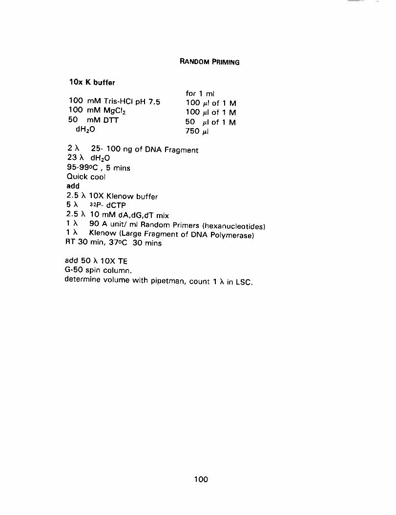
RANDOMPRIMING
l Ox K buffer
100 mM Tris-HCI pH 7.5
100 mM MgCI250 mM DTT
dH20
for 1 ml
100 FI of 1 M
lO0/_lof 1 M
50 /_1 of 1 M
750 #1
2 ;k 25- 100 ng of DNA Fragment
23 k dH20
95-99oC, 5 mins
Quick cool
add
2.5 ;k IOX Klenow buffer
5 ;k 32p_ dCTP
2.5 k 10 mM dA,dG,dT mix
1 X 90 A unit/ ml Random Primers (hexanucleotides)
1 X Klenow (Large Fragment of DNA Polymerase)
RT 30 min, 37oC 30 rains
add 50 ;k 1OX TE
G-50 spin column.
determine volume with pipetman, count 1 X in LSC.
100
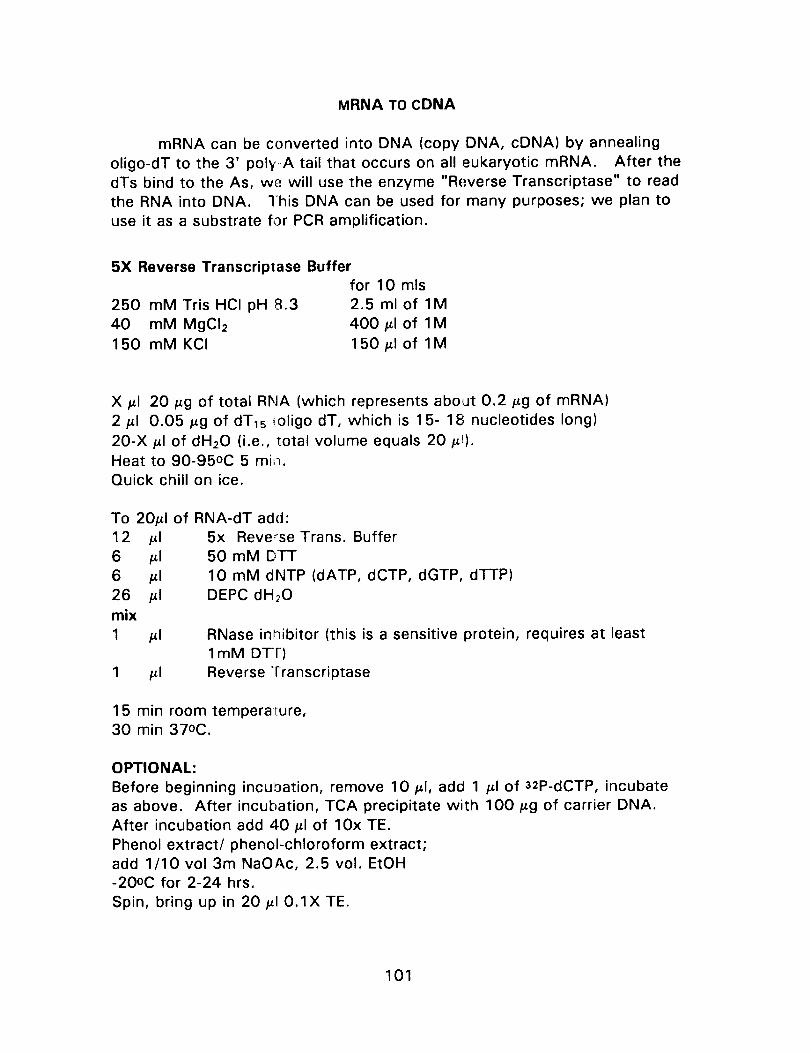
MRNA TO CDNA
mRNA can be converted into DNA (copy DNA, cDNA) by annealing
oligo-dT to the 3' poly-A tail that occurs on all eukaryotic mRNA. After the
dTs bind to the As, we will use the enzyme "Reverse Transcriptase" to read
the RNA into DNA. "lhis DNA can be used for many purposes; we plan to
use it as a substrate for PCR amplification.
5X Reverse Transcriptase Bufferfor 10 mls
250 mM Tris HCI pH 8.3 2.5 ml of 1M
40 mM MgCI2 400 #1 of 1M
150 mM KCI 150#1of 1M
X #1 20 #g of total RNA (which represents about 0.2 #g of mRNA)
2 #1 0.05 #g of dT15 _oligo dT, which is 15- 18 nucleotides long)
20-X #1 of dH20 (i.e., total volume equals 20 #t).Heat to 90-95oC 5 min.
Quick chill on ice.
To 20#1 of RNA-dT add:12
6
6
26
mix
1
#1
#1
#1
#1
5x Reve'se Trans. Buffer
50 mM DTT
10 mM dNTP (dATP, dCTP, dGTP, dTTP)
DEPC dH20
#1
#1
RNase inhibitor (this is a sensitive protein, requires at least
I mM DTF)
Reverse Transcriptase
15 min room temperature,
30 min 37oC.
OPTIONAL:
Before beginning incuoation, remove 10 #1, add 1 #1 of 32P-dCTP, incubate
as above. After incubation, TCA precipitate with 100 #g of carrier DNA.
After incubation add 40 #1 of 10x TE.
Phenol extract/phenol-chloroform extract;
add 1/10 vol 3m NaOAc, 2.5 vol. EtOH-20oC for 2-24 hrs.
Spin, bring up in 20 #1 0.1X TE.
101
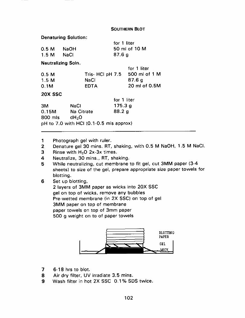
Denaturing Solution:
0.5 M NaOH
1.5 M NaCI
Neutralizing Soln.
0.5M
1.5M
0.1M
20X SSC
SOUTHERN BLOT
for 1 liter
50 ml of 10 M
87.6 g
Tris- HCI pH 7.5NaCI
EDTA
3M NaCI
0.15M Na Citrate
800 mls dH20
for 1 liter
500 ml of 1 M
87.6 g20 ml of 0.5M
for 1 liter
175.3 g
88.2 g
pH to 7.0 with HCI (0.1-0.5 mls approx)
1
2
3
4
5
6
Photograph gel with ruler.
Denature gel 30 mins. RT, shaking, with 0.5 M NaOH, 1.5 M NaCI.
Rinse with H20 2x-3x times.
Neutralize, 30 mins., RT, shaking.
While neutralizing, cut membrane to fit gel, cut 3MM paper (3-4
sheets) to size of the gel, prepare appropriate size paper towels for
blotting.
Set up blotting,
2 layers of 3MM paper as wicks into 20X SSC
gel on top of wicks, remove any bubblesPre-wetted membrane (in 2X SSC) on top of gel
3MM paper on top of membrane
paper towels on top of 3mm paper
500 g weight on to of paper towels
7
8
9
6-18 hrs to blot.
Air dry filter, UV irradiate 3.5 mins.Wash filter in hot 2X SSC 0.1% SDS twice.
102
HYBRIDIZATIONS: RNA OR DNA
2X Hybridization soln.
10X SSPE
lOX Denharts
0.2 %SDS
Denhardt's soln.
Ficoll
polyvinylpyrrolidone
BSA (fraction V)
20X SSPE
3.6 M NaCI
0.2 MPhosphate pH 7020 mM EDTA
Phosphate Buffer pH 7.0
Na H2PO4 (monobasic)
Na2 H PO4 (dibasic)
Hybridization soln. (HB)
for 100 ml
50 ml of 20X
20 ml of 50X
2 mJ of 10%
for 100 ml
lg
lg
lg
for 500 ml
105.2 g100 ml of 1 M
20mlof 0.5 M
for 500 ml
140 ml of 1 M
360 ml of 1 M
Make fresh when needed. Denature DNA by boiling 5 rainsDeionize foramide with mix bed resin (Biorad AG-501-XS)
10 mls of 2x
10 mls of foramide
1 mg of sonicated denatured DNA (calf thymus, salmon sperm)for Northerns
500/_g of clean (Prot. Kase, Phenol) yeast RNA.
Use HB, to pre-hybridi;,e 6 to 12 hrs; less if lots of target DNA.
Add probe directly to HB soln. Hybridize 12 to 36 hours depending on
amount of probe, qualitative vs. quantitative results and amount of target.
After hybridization,
Empty hot soln. into waste container, rinse with minimum vol of 2X SSPE
0.1% SDS, twice, putting rinse into waste.
(You want to minimize the amount of hot waste you produce.)Wash 2X SSPE 0.1% $DS, 65oC 15 min twice
Wash0.2XSSPE0.2% SDSRT 15 min
103

RNA DOT BLOT
1
2
3
4
5
6
7
8
9
Prewet 2 sheets of 3MM and 1 sheet of nylon membrane, cut to thesize of dot blotter.
Place paper and membrane into dot blotter, membrane on top.
Low negative pressure add 0.1% solution of India ink to upper rightcorner.
Sample prep: heat 2 -10 #g of total RNA to 65oC, 10 min, quick cool,
add 2.5 vol DNA denaturing reagents. Add 1-2 #1 of 1% loading dyes
(dyes make it easier to tell if you have loaded a sample successfully).Include some yeast DNA as a negative control.
cRNA: prepare sample as above using a serial dilution from 200 pg to 2
pg (dilute in a solution of yeast RNA so total nucleic acid is constant).
Load sample onto blotter, be sure there is not an air lock (use pipetmanto remove air).
After blotting, air dry, wash in 5X SSC 0.5% SDS, RT 10 mins.UV irradiate 3.5 rains.
Wash in hot 2X SSC 0.1% SDS, twice.
Prehybridize 12+ hours, hybridize 24 + hours.
10 Wash as before for Northern/southerns.
11 Autoradiograph 12 hours.
After
12
13
14
15
16
17
Autoradiography,
Label 3 ml scintillation tubes for samples.
Add 400/_1 of 0.1 N NaOH to tubes.
Carefully add equal size cut out dots to tubes, plus some negativecontrols.
Incubate 37oC 15 mins, cool, add 2.5 mls of LSC fluid, mix well.Let sit for 30 minutes.
Count for four minutes, twice (repeat counts after all samples have
been counted, greater than 1 hour between first and second). Are thecounts for each sample the same?
104

T4 DNA Polymerase
To be sure you hav_ a blunt end (e.g., on PCR product) or to convert 3' and
5' overhangs to blunt ends, use T4 DNA polymerase with 0.5 mM dNTP.
l OX T4 buffer
0.5 M l-ris-HCI pH 8.0
50 mM Mg CI250 mM OTT
100/_g/ml i-3SA
for 10 ml
5 ml of 1 M
500/_1of 1 M
500/_1of 1 M
100/_1 of mg/ml
Reaction:
up to 2 #g !_)NA
4/_1 I OX T4 buffer
2/_1 10 mM dNTP
dH20 up to 39 #1
1 /_1to T4 DNA polymeraseincubate 30 minute_ 37oC
Note: read page 3.5.11-12 in "Red Book" for more details
up to 2/zg
105

Media for Bacteria
LB:
for 1 liter
10 g Tryptone
5 g yeast extract
5 g NaCI
100/_1 10 N NaOH
Superbroth:for 1 liter
20 g Tryptone
10 g yeast extract
5 g NaCI
500 #1 10 N NaOH
Additives:
final stock
Ampicillin 100 #g/ml 50 mg/ml
Kanamycin 70 #g/ml 35 mg/ml
Tetracycline 15 #g/ml 15 mg/ml
add
2/_l/ml
2/_l/ml
light sensitive in 70% EtOH
(Do not use with media containing MG)
X-Gal 25/_g/ml 25 mg/mlIPTG O. 1 mM 100 mM
1 #l/ml
1 #l/ml
1 #l/ml
Plates:
15 g/liter for agar plates.
Add additives only when media cools to approximately 50 to 55oC.
Most all plasmids have AMP resistant genes, and so need to be grown in
media with ampicillan.
XL-1 has a special episome with Tet resistance for blue-white selection and
for the production of single-stranded DNA; therefore, use tetracycline when
growing up XL-I.
When plating a recombinant plasmid (one in which you hope to have cloned
a piece of DNA into the polylinker) you will disrupt the _-Iac gene and thus
the bacteria (DH-5 a, or L1-1) cannot turn X-Gal blue. Therefore, whitecolonies should be recombinants.
106

Preservation of Animal Tissue at Room Temperaturefor DNA Analyses
(from Seutin, et al., Can. J. ZooL 69:82, 1991)
This protocol has worke¢ well for finely minced tissues and cell suspensionsfrom fish and invertebrat,_s.
DMSO-salt solution:
20% DMSO
0.25 M sodium-EDTA
NaCI to saturation
pH to 7.5 with HCI or NaOH
1. Cut up tissue to rice-size pieces or grind up soft tissues between two
frosted slides to make a cell suspension.
2. Immerse in DMSO-salt solution (at approx. 1 g tissue per 3 ml). Leave at
room temperature, up to 24 weeks.
3. Remove excess superr, atant (tissue and cells will be pelleted by gravity).
Grind up in liquid nitroger_. Add DNA lysis buffer and follow DNA isolationprotocol.
107

Geneclean: the Wonders of Glass and DNA
1. Excise band from agarose from gel, estimate vol. and put into labeled
microfuge tube. Note: minimize the amount of agarose gel.
2. Add 3 vol. of Nal stock (incubate 5 rain. at 50oC). Make sure the gel
slice is dissolved.
3. Add 5/_1 of Glassmilk, incubate for 5 rain. at room temperature.
Glassmilk is a solution of very fine (small) glass particles that bind DNA.
4. Spin solutions for 5 seconds to pellet glass particles with DNA bound to
glass. Note: if you spin too long you will not get your DNA back.
5. Remove supernatant, put into separate tube (most likely will not use the
supernatant).
6. Resuspend pellet in "New Wash" by vortexing.
7. Spin again for 5 seconds.
8. Remove supernatant.
9. Repeat steps 6-8 two more times.
10. After last wash, remove all of wash solutions. To be sure you remove
all of wash solutions, spin for 2 seconds and remove any remaining liquid.
11. To elute DNA from Glassmilk, add 10/_1 of dH20, vortex to resuspend,
incubate at 55oC for 10 min.
12. Pellet the Glassmilk by microfuging for 30 seconds (you want a firm
pellet).
13. Remove supernatant, which has the DNA in it, and put into fresh tube.
14. Repeat steps 11-12 and combine eluent in one tube for a total volume
of 20/_1.
Assume 80% yield when estimating DNA concentrations.
108

STET:8% sucrose0.5% Triton X-lO050 mM EDTA50 mM Tris-CI pH 8.0
Boiling Minipreps for Plasmid DNA
RNase
Lysozyme
IsopropanolTE
1. Take pellet from 1.5 mls of overnight culture and resuspend in 300 #1
STET with 200/zg of lysozyme. Vortex well.
2. Place on ice for 30 sec. - 10 min.
3. Place in boiling water bath for 1-2 min.
4. Spin for 15-3(3 min. Pull out pellet with toothpick and throw away.
5. Add 1 volume of isopropanol, leave at -2OOC for 15-30 min.
6. Spin for 5 mir_. Remove supernatant and dry briefly.
7. Resuspend in 50 #1 of TE. Digest 5/zl with appropriate restriction
enzymes and 1 # of 10 mg/ml RNase.
109

Lecturers' Abstracts and References
Edward DeLong
Ann Giblin
Robert Haselkorn
Thomas Hollocher
Stephen Macko
Donal Manahan
Joseph Montoya
Daniel E. Morse
Kenneth H. Nealson
Sandra Nierzwicki-
Bauer
David L. Peterson
Thomas Schmidt
Simon Silver
Mitchell L. SoginIvan Valiela
Appendix:
Fluorescent Labeling of Amino-Oligonucleotides
Application of Molecular Genetic Techniques to
Microbial Ecology
Overview of the Importance of Subtidal Sediments
to Nitrogen Cycling in Coastal Environments
The Importance of Benthic Macrofauna to Decom-
position and Nitrogen Cycling in Sediments
Heterocyst Differentiation and Nitrogen Fixation
in Cyanobacteria
Enzymes of Nitrification and Denitrification:
Parts of the Global Nitrogen Cycle
Use of Bulk Stable Isotopes for Environmental
Studies: Stable Isotopes at the Molecular Level
Energy Metabolism During Larval Developmentand Animal/Chemical Interactions in the Sea
Stable Isotopes and Their Use in BiogeochemicalStudies
Molecular Mechanisms Controlling Settlement and
Metamorphosis of Marine Invertebrate Larvae
Ecology of Luminous BacteriaMolecular Methods for the Identification and
Analysis of Phylogenetic Relationships Among
Subsurface Microorganisms
Gene Expression in Symbiotically Associated and
Free-Living Cyanobacteria
Remote Sensing of Ecosystems and Simulation of
Ecosystem Processes
Molecular Phylogenies and Microbial Evolution
Identification and Quantification of Microorganisms
in Natural Habitats Using rRNA-Based Probes
Transport Across the Cell Surface: GoodSubstrates and Bad
Biochemistry and Molecular Biology of Bacterial
Resistances to Toxic Heavy Metals
Metallothioneins: Small Cadmium-Binding Proteins
from Horses, Plants and Bacteria
Recent Developments in Phylogeny of Eukaryotes
An Overview of Nitrogen Cycling in Marine and
Aquatic SystemsAbbreviations
111
117
122
123
125
128
133
138
139
141
143
146
147
148
159
160
163
164
165
167
169
170
110
Edward DeLongUniv. of California-Santa Barbara
Fluorescent Labeling of Amino-Oligonucleotides
Oligonucleotides that have a free amino group at their 5' ends are
readily synthesized on automated DNA synthesis machines, using
commercially available amino modifying reagents (Aminolink I and II, Applied
Biosystems). These amino-oligonucleotides can then be further labeled with
a fluorophore, biotin, or other reagent via the free amino group. The
following protocol is useful for labeling oligonucleotides with isothiocyanate
(Fluorescein-ITC) or sulfonyl chloride (Texas Red) dyes, for use in in situ_
hybridizations.
[Editor's Note: Dr. Ed DeLong was an active participant
in the laboratory part of our course. He presented lab
demonstrations of the use of hybridization probes for the study
of environmental biology. In addition, he presented a short
lecture outlining some of the uses of these new techniques,
and some of the questions that can and cannot be answered
using these approaches. The students requested that Dr.
DeLong's laboratory protocols, as well as the overhead
projections from his lectures, be included in this document.
These are in a slightly different format from the lecture
abstracts, but they do present in outline form what was
discussed in the lecture part of this laboratory session.]
Labeling Reaction
1) Dry 100/_g of gel purified amino-oligonucleotide. Purify the aminolink
oligo on a nondenaturing 20% acrylamide preparative gel. An 18met runs
between the xylene cyanol and bromphenol blue. After electrophoresis,
locate the oligo by its UV shadow (cast on a fluorescent TLC plate or
intensifying screen). Excise the band from the gel and place it in a small
vial. Add 1-2 ml sterile dH20 and elute (with rotation or agitation)
overnight. Remove the eluate and filter through a 0.2 vm filter. Measure
the A260 to quanti_ate the recovery.
2) Add 200 #1 of 50 mM Borate Buffer pH =9.2 (or 50 mM Carbonate
Buffer). Check the pH of the reaction with pH paper. It's important that the
pH is greater than 9.0.
Borate Buffe_ pH = 9.2
Solution A = 0.1 M H3BO3
Solution B = 0.1 M NaOH
For 50 mM Borate Buffer: mix 50 ml Solution A and 26.4 ml Solution B.
Bring volume to 100 ml with dH20 and check pH.
111
3) Add 40 #1 of Stock Dye (Stock Dye = 10 mg dye dissolved in 1 ml
dimethylformamide). Make dye fresh each time. Molecular Probes (Eugene,
Oregon) sells 1 and 10 mg ampules of dye, which are opened, dissolved in
DMF, used once, and discarded.
4) Place reaction in dark, overnight. In the subsequent handling of the fluor
labeled oligonucleotide, avoid excessive exposure to light.
5) Prepare Sephadex G-25 by hydrating it in 10 mM Tris HCI, pH=7.5. Let
the Sephadex hydrate overnight.
Removing Unincorporated Dye
6) Set up one column of Sephadex G-25 for each reaction. (Plastic 10 ml
disposable pipettes, plugged with glass wool, work well.) A bed volume of
5-7 ml provides good separation of oligo from unincorporated dye. Collect
about 4 drop fractions in a microtiter plate or in epi-tubes. The labeled
oligonucleotide is visible as a colored band, and should elute in the void
volume, well separated from the intensely fluorescent trailing band, which is
the unincorporated fluor.
7) Examine the collected fractions under a long wave UV lamp. The first
fluorescent peak is the labeled oligonucleotide. Pool these fractions.
8) Lyophilize the pooled product in a Speed-vac or the equivalent.
Resuspend in 8 M urea, or 80% formamide, to increase the density for gel
loading.
Separating the Labeled from Unlabeled Oligonucleotide
9) Load the product onto a preparative, 20% (5% x-link) nondenaturing
acrylamide gel. A gel thickness of 2 mm is appropriate for purifying the 100
#g reactions. An oligomer 18 nucleotides in length will run approximately
halfway between the xylene cyanol and bromphenol blue in this gel system.
Load some xylene cyanol and bromphenol blue into an empty lane to serve
as markers. It's a good idea to also run some labeling dye (e.g., FITC,
Texas Red) to see where unincorporated dye runs. Electrophorese at 25W
constant power for about 4 hours.
10) Visualize the unlabeled oligomer by the shadow it casts when it is
placed on a fluor-impregnated TLC plate (covered with Saran Wrap) and
illuminated with UV light (can also use an intensifying screen as a backing
to locate the UV shadow). The labeled product should be slightly above the
"shadow" band -- the fluor retards the migration of the oligomer by
approximately 1 nucleotide. Excise the fluorescently labeled product, and
112
place the gel slice in aboul 1 ml ddH20. Allow the product to elute from the
gel overnight, preferably with agitation. Remove the eluate, and filter out
the acrylamide (0.22 #m acrodiscs or similar disposable filters work well).
Measure the A26o and the Area, of the fluor (495 nm for fluorescein).
A26o/Aflourm_x is about 3.0-3.5. Yields are usually about 20-30 #g of pure,
labeled oligonucleotide. Store the purified, labeled oligo frozen at -20oC, in
small aliquots of one to a few micrograms.
in Situ Hybridization with
rRNA-Targeted Fluorescent Oligodeoxynucleotides
MATERIALS
50 ml Falcon tubes
staining jarsslide racks
teflon coated slides (Cell I.ine Associates, Newfield, N J)
pipetmen p-20, p-200, p-1000
water bath and dry incubator
coverslips
Citifluor mountant (or gly,;erol:PBS [9:1])immersion oil
epifluorescence microsco_)e
Gelatin Subbed Slides:
Soak clean slides for 2 minutes in a filtered 65oC solution of:
0.1% gelatin
0.01% CrK(SO4)2 (chrom alum)
Air dry
REAGENTS
1X phosphate buffered sl]line (PBS) (pH =7.6)methanol
37% formaldehyde (or fr._,shly prepared 8% paraformaldehyde in lX PBS)
2 M Tris, pH =7.8
2% BSA (fraction V)25X SET:
3.75 M NaCI
25 mM EDTA
0.5 M Tris, pH =7 810% SDS
distilled H20
rRNA targeted, fluor-labeled oJigodeoxynucieotide probes
113
PROTOCOL
1) Cell Preparation
Centrifuge cell sample, and resuspend in PBS (1/2 X artificial
seawater, if of marine origin). Cells can then be fixed by adding 1/10
volume of 37% formaldehyde, followed by storage for 4-16 hours at 4oC.
Cells may then be resuspended in 1X PBS buffer and stored at 4oC for up to8 weeks.
Alternatively, freshly grown or collected cells may be spotted directly
onto "subbed" slides. These can be fixed (as described in step two), dried,
and stored indefinitely.
A good concentration for cell suspensions to be smeared is
approximately 1X10⁷ cells/ml. Again, one can use cells previously fixed in
3.7% formaldehyde/IX PBS. Spot 10 _1 of the well-mixed cell suspension
directly onto the slide. Use the backside of a 200 #1 pipette tip to spread
the cells. Let the smear air dry.
2) Post-Fixation
Place slides in a slide rack. Set in a staining jar containing a mixtureof methanol:formaldehyde, 9:1. (Final concentration of formaldehyde is
3.7%). Incubate at room temperature 20 minutes. Remove slides and dip
briefly in H20 to rinse. Air dry.
3) Hybridization Buffer (make fresh, as follows:)
Stock reagent Volume to add
dH20 2.76 ml
25X SET 800 /_1
2% BSA (optional) 400 #1
10% SDS 40 #1
Final Conc.
5X SET
0.2% BSA
0.1% SDS
4) Hybridization
Lyophilize enough fluor-labeled oligodeoxynucleotide probe for 50 ng
probe/smear. Resuspend the probe in Hybridization Buffer (above) to a final
concentration of 5.0 ng probe/_l in Hybridization Mix (from above). 10/_1 of this
probe dilution is used per smear, for a total of 50 ng probe/smear. Mix probe
and hybridization mix gently by tapping the tube lightly -- try to avoid vigorousagitation and bubble formation.
Add 10/_1 of the appropriate probe onto each of the smears, directly on
top of the cell smear. Next the slides are carefully placed in an airtight
chamber containing a tissue soaked in Hybridization Buffer, to prevent drying
of the probe-hybridization mixture. For single slides, 50 ml Falcon tubes
make convenient hybridization chambers. Place the slide in a 45oC dry type
incubator, and hybridize from 2 hours to overnight. (The hybridization and
wash temperatures are determined empirically for each different probe.)
114

5) Washes (Can be dora; after 2-16 hours of hybridization.)
Set up a staining jar in the 45oC waterbath (the wash temperature will
depend on the particular probe being used) and fill it with pre-equilibrated
0.2X SET. Place the hybridization slides in the O.2X SET. Note the time;
after 10 minutes, pour off the 0.2X SET and replace with fresh 0.2X SET.
Wash for 10 more minutes, and again replace with fresh O.2X SET. After a
final 10 minutes, remove slides and allow to air dry in subdued light. When
slides are dry, place a small drop of mountant directly on the smear, cover
with a coverslip; view _ia epifluorescence microscopy.
References:
Amann, R.I., L. Krumholz, and D.A. Stahl (19901 Fluorescent-
oligodeoxynucleotide probing of whole cells for determinative, phylogenetic
and environmental studies in microbiology. J. BacterioL 172:762-770.
Amann, R.I., B.B. Binder, R.J. Olson, S.W. Chisholm, R. Devereux, and D.A.
Stahl (1990) Combination of 16S rRNA-targeted oligonucleotide probes with
flow cytometry for analyzing mixed microbial populations. AppL Environ.MicrobioL 56:1919-1925.
Amann, R.I., N. Springer, L. Ludwig, H. Gortz, and K.H. Schleifer (1991)
Identification in situ and phylogeny of uncultured bacterial endosymbionts.Nature 351:161-164.
DeLong, E.F., G.S. Wi(;kham, and N.R. Pace (1989) Phylogenetic stains:
Ribosomal RNA-based [)robes for the identification of single cells. Science243:1360-1363.
DeLong, E.F., and J. Shah (1990) Fluorescent ribosomal RNA probes for
clinical application: a research review. Diagnos, Clinc. Test, 28:41-44.
Distel, D.L., E.F. DeLong, and J.B. Waterbury (1991) Phylogenetic
characterization and it. situ localization of the bacterial symbiont of
shipworms (Teredinid_e Bivalvia) using 16S rRNA sequence analysis and
oligodeoxynucleotide probe hybridization. AppL Environ. MicrobioL57:2376.
Giovannoni, S.J., E.F. DeLong, G.J. Olsen, and N.R. Pace (1988)
Phylogenetic group-specific oligodeoxynucleotide probes for identification of
single microbial cells. J. BacterioL 170:720-726.
115

Lane, D.J., S.J. Giovannoni, and N.R. Pace (1986) Microbial ecology and
evolution: A ribosomal RNA approach. Ann. Rev. MicrobioL 40:337-355.
Stahl, D.A., and R.I. Amann (1991) Development and application of nucleic
acid probes. In: Nucleic Acid Technique_ in Bacterial Systematics. E.
Stackebrandt, and M. Goodfellow (eds.) J.W. Wiley and Sons, New York,
pp.205-248.
Tsien, H.C., B.J. Bratina, K. Tsuji, and R.S. Hanson (1990) Use of
oligodeoxynucleotide signature probes for identification of physiological
groups of methylotrophic bacteria. AppL Environ. MicrobioL 56:2858-2865.
116

Edward DeLong
Application of Molecular Genetic Techniques
to Microbial Ecology
[overheads from lecture]
BIODIVERSITY & COMMUNITY STRUCTURE:
WHO'S OUT THERE???
POPULATION STABILITY & DYNAMICS:
HOW DO POPULATIONS CHANGE,
& WHAT FACTORS CONTROL VARIABILITY?
ORGANISMS to PROCESSES:
WHO'S DOING WHAT (AND HOW)?
ORGANISMAL ADAPTATIONS/INTERACTIONS
117

BIODIVERSlTY/COMMUNITY STRUCTURE:
WHO'S OUT THERE?
SPECIFIC QUESTIONS:
What is the species composition of specific microbial populations?
Do we ignore a significant fraction of extant microbial diversity?
On what spatial scale are communities appropriately defined?
POTENTIALLY USEFUL MOLECULAR APPROACHES:
Cloning and sequencing of phylogenetically informative genes
from mixed, microbial assemblages
Identification of species or groups with nucleic acid probes
Identification of species or groups with immunological probes
118

POPULATION STABILITY & DYNAMICS:
HOW DO POPULATIONS CHANGE, &
WHAT FACTORS CONTROL VARIABILITY?
SPECIFIC QUESTIONS:
How do individual species vary in time and space?
What are the major factors controlling this variability?
PhysicalTemperature
Light
Pressure
ChemicalNutrients
Anthropogenics
Redox
BiologicalPredation
Viral infection
Syntrophy/symbiosis
What is the extent and role of intraspecific variability?
POTENTIALLY USEFUL MOLECULAR APPROACHES:
Identification and enumeration using nucleic acid probes
Identification and enumeration using immunological probes
Molecular analyses of acclimation and stress responses
RFLP analysis of intraspecific genetic variability
Nucleic acid sequence analyses of genetic variability
119

ORGANISMS to PROCESSES:
WHO'S DOING WHAT?
SPECIFIC QUESTIONS:
Can functional roles be inferred from phylogenetic affiliations?
Can organism variability be correlated with process variability?
Can we monitor the expression and regulation of functional genesin the environment?
Regarding regulation of specific processes in the environment,what are the relative roles of:
1) Major changes in community structure
2) Intraspecies variability and selection of genetic variants
3) Intracellular regulatory circuits
POTENTIALLY USEFUL MOLECULAR APPROACHES:
Monitoring species variability with probes (& correlations withenvironmental activities)
Measure environmental gene expression with mRNA specific or
immunological probes
Follow induction of reporter genes in genetically engineered
organisms
Molecular analyses of intracellular regulatory circuits
120

ORGANISMAL ADAPTATIONS/INTERACTIONS
SPECIFIC QUESTIONS:
What specific adaptations are required, at the genetic and
molecular level, for optimal function in unique marine
habitats?
What is the role of gene regulation in acclimation/adaptive
responses?
What molecular mechanisms are responsible for recognition,
communication, and maintenance of host/symbiont
relationships?
POTENTIALLY USEFUL MOLECULAR APPROACHES:
Structure/function comparison of nucleic acid and protein
sequences
Gene fusion experiments for monitoring gene regulation
Genetic analysis of mutants/variants in host/symbiont studies
Use of molecular probes to follow symbiont transmission to host
progeny
121
Ann GiblinWoods Hole Ecosystems Center
An Overview of the Importance of Subtidal Sediments to Nitrogen Cycling
in Coastal Ecosystems
A variety of evidence has shown that the primary production of most
nearshore coastal ecosystems is limited by nitrogen. For example, there is a
strong relationship between nitrogen loading and primary production in
estuarine ecosystems (Boynton et aL, 1982; Nixon and Pilson, 1983). In
contrast, phosphorous appears to be the most limiting element for primary
production in freshwaters. A variety of reasons for the differences between
freshwater and marine systems have been proposed. Howarth et aL (1988)
have suggested that the greater importance of planktonic nitrogen fixation in
freshwater may explain why freshwaters are more likely to be P limited.
The sediments play an important role in recycling nitrogen in coastal
ecosystems. Nitrogen is deposited onto the sediments as particulatedetritus where it is mineralized to ammonium and diffuses into the water
column, then becoming available for uptake by plankton. The amount of
recycling varies considerably among systems (Boynton et aL, 1982; Kelly, in
press), but in most estuaries and coastal systems nitrogen is used several
times before it is lost by flushing, burial, or conversion of N2.
Burial of nitrogen in sediments is fairly low; usually less than 10% of
the annual nitrogen input to the sediments is buried. In contrast, losses by
denitrification have been reported to be high. Seitzinger (1988) has
estimated that 20-70% of the nitrogen input to the sediments may be lostvia denitrification.
To predict the magnitude and seasonal cycle of primary productivity it
is necessary to understand the controls on nitrogen release from sediments.
A seasonal study at one site in Buzzards Bay showed that most of the
variation in nitrogen release from the sediments could be explained by
temperature and phaeopigment concentration (Banta, 1991). In contrast,
much of the difference between sites can be explained by differences in
input to the sediments and the amount of denitrification (Banta, 1991; Kelly,
in press).
There are two mechanisms by which denitrification takes place in
sediments. In some sediments nitrate is taken up by the overlying waterand denitrified. The controls on this mechanism of denitrification are the
nitrate concentration of the overlying water and organic matter availability
of the sediments. The more important mode of denitrification is couplednitrification/denitrification. In this case, mineralized ammonium is nitrified in
the oxic portions of the sediments. A portion of this nitrate diffuses into the
anoxic areas of the sediments where it is subsequently denitrified. (See
Vanderborght et aL,1977 for a model of this process.) Controls on this
process are complex and include the depth of the oxic layer, the irrigation
122

rate of the sediment, arid the availability of organic matter below the oxiclayer.
A gradient from 1he sewage outfall in Boston Harbor toMassachusetts Bay illustrates how the importance of these two modes ofdenitrification change with organic matter loading (Giblin et a1.,1990). In
Boston Harbor, sedimm_ts are anoxic to the surface and take up nitrate from
the overlying water. In Massachusetts Bay the sediments have a well
developed and bioturbated oxic layer. These sediments release both nitrate
and ammonium. The ratio of oxygen consumed to nitrogen released
suggests that a substar_tial amount of the N mineralized in these sediments
is lost via denitrificatior_.
The Importance of Benthic Macrofauna to Decomposition and
Nitrogen Cycling in Sediments
Benthic macrofauna have the potential to change the decomposition
and cycling rates in sediments through their activities (Aller, 1982). By
building irrigation burrows animals change the availability of oxygen in the
sediments and remove potentially inhibitory end-products. Macrofauna
redistribute particles, break them up, and repackage them into fecal pellets.
It has been proposed that by grazing senescent bacteria from particles,
macrofauna increase decomposition rates by keeping microbes in log-phase
growth. Animal activities also change sediment surface characteristics and
alter resuspension. In !aboratory experiments, adding macrofauna to
decomposing detritus _sually increases decomposition rates (Aller, 1982).
Recent experiments by Banta (1991) have indicated that the role of
macrofauna in altering decomposition rates may be more complicated than
previously believed. When macrofaunal populatuons were manipulated insediment taken from Buzzards Bay in the summer, the presence of benthic
animals increased decomposition by magnitudes of 2 to 3; however, whensediments were taken from the field in the fall, the macrofauna had no
effect on decomposition. Macrofauna did change porewater irrigation in
both experiments. To test whether the substrate quality in sediments
explained the difference between the two experiments, Banta (1991)
manipulated both orgarfic matter and macrofauna numbers. When organic
matter quality was very low or very high macrofauna did not alter
decomposition rates. Macrofaunal stimulation of decomposition did occur
when organic matter was of intermediate quality.
123

References:
Aller, R.C. (1982) The effects of macrobenthos on chemical properties ofmarine sediment and overlying water. In: Animal-Sediment Relations. The
Biogenic Alteration of Sediments. P.L. McCall, and M.J.S. Tevesz (eds.)pp.53-102.
Banta, G.T. (1991) Decomposition and nitrogen cycling in coastal marine
sediments: Controls by temperature, organic matter inputs, and benthic
macrofauna. Ph.D. dissertation, Boston University.
Boynton, W.R., W.M. Kemp, and C.W. Keefe (1982) A comparative analysis
of nutrients and other factors influencing estuarine phytoplankton
production. In: Estuarine Comparisons. V.S. Kennedy (ed.) pp.69-90.
Giblin, A.E., J.Tucker, and C. Hopkinson (1991) Sediment oxygen demand
and nitrogen flux in Massachusetts Bay. Massachusetts Water Resources
Authority, Final Report, June, 1991.
Howarth, R.W., R. Marino, J. Lane, and J.J. Cole (1988) Nitrogen fixation in
freshwater, estuarine, and marine ecosystems. 1. Rates and importance.LimnoL Oceanog. 44:669-687.
Kelly, J.R. (in press) Paradigms of benthic-pelagic coupling of carbon andnutrients in coastal ecosystems as derived from annual field studies. J.Mar. Res.
Nixon, S.W., and M.E.Q. Pilson (1983) Remineralization and nutrient cycling
in coastal marine ecosystems. In: Nitrogen and the Marine Environment.
B.J. Neilson, and L.E. Cronin (eds.) pp.565-648.
Vanderborght, J.P., P. Wollast, and G. Billen (1977) Kinetic models of
diagenesis in disturbed sediments. 2. Nitrogen diagenesis. LimnoLOceanog. 22: 794-803.
124

Robert HaselkornUniversity of Chicago
Heterocyst Differentiation and Nitrogen Fixation in Cyanobacteria
Cyanobacteria are ubiquitous prokaryotes that cover Earth, inhabiting
the oceans, streams, ponds, soil and rock surfaces. They carry out green
plant photosynthesis, liberating oxygen in the light. Many species also
convert atmospheric nitrogen to ammonia, enabling them to live and
reproduce in environments that provide little more than phosphate, sulfate,
and a few metal ions. Most nitrogen fixing cyanobacteria grow in long
filaments of more than 100 cells. When nitrate or ammonia are abundant,
all the cells look the same. When these sources of nitrogen are limiting,
cells specialized for nitrogen fixation differentiate at regular intervals alongthe filament. In our strain of Anabaena, approximately every tenth celldifferentiates.
Anabaena vegetative cells contain 10-20 copies of a circular
chromosome of 6.4 Mb. We estimate, on the basis of RNA hybridization
studies, that 20-25% of the chromosome, corresponding to 1200-1600
genes, is required for the processes of heterocyst differentiation and
nitrogen fixation.
To characterize these genes we haw,, taken three approaches: cloning
and analysis of genes known to be differentially regulated; isolation of
developmental mutants and the genes that complement those mutations;
and the brute force description of clones in stage-specific cDNA libraries
prepared from mRNA populations. Each approach has yielded some
unexpected results; one example of each will be described.
Nitrogen fixation is accomplished by the enzyme complex called
nitrogenase, which contains three different polypeptides, several iron-sulfur
clusters, and cofactors of iron, sulfur, and molybdenum. The nitrogenase
polypeptides are encoded by three genes called ni._!fH, ni__!fD,and nifK which,
in most diazotrophs, are co-transcribed in the order ni___fHDK. This operon is
not transcribed in cells growing on ammonia or in the presence of oxygen,
due to a requirement of the ni__fHpromoter for activation by a DNA-binding
protein (NifA) that is not present or not functional except under nitrogen
starvation, anaerobic conditions. One of the reasons for heterocyst
differentiation is to provide a locally anaerobic environment for both ni_ffgene
expression and nitrogenase function. When we originally cloned and
sequenced the ni.__ffH,D, and K genes from the DNA of Anabaena vegetative
cells, we were surprised to find an 11-kb element interrupting the coding
sequence of the nifD gene. The presence of this element would make it
impossible to transcibe the ni__[fKgene and therefore impossible to fixnitrogen. Subsequently, it was discovered that the 11-kb element is excised
from the chromosome during heterocyst differentiation by site-specific
recombination between directly repeated sequences at the ends of the
125

element. The excision reaction results in the formation of a non-replicating
11-kb circular DNA molecule and a fused chromosome, in which the nifHDK
operon is restored with an intact ni._!D reading frame. The restored operon is
the template for synthesis of nifHDK messenger RNA.
The excision reaction is catalyzed by a recombinase enzyme encoded
within the 11-kb element itself. Mutation of the xi___ssAgene prevents excision
and results in a Nif-phenotype. The 11-kb element is widely distributed in
free-living Anabaena, having been identified in newly isolated strains from
India, Costa Rica, and the U.S. Since the element must be excised for the
strain to survive nitrogen starvation, there must be another function it
encodes that provides a selective advantage to cells carrying it. That
function is still unknown, although it has been guessed to be a phage
immunity substance, a restriction activity, or a DNA repair activity.
Since nitrogen fixation requires the anaerobic milieu and other
properties of the heterocyst, Anabaena mutants affected in heterocyst
development are unable to grow on N2 as nitrogen source in air. It has
therefore been possible to design a penicillin-selection scheme, based on the
Nif-phenotype, to select mutants defective in heterocyst differentiation.
There are many morphological classes of mutants, including one that makes
too many heterocysts, one that makes too few (only at the ends offilaments) and one that makes none. To illustrate this approach, the latter
will be described further.
Mutant 216 grows perfectly well on nitrate or ammonia as nitrogen
source. Starved of nitrogen, it turns yellow and dies. It does not initiate
heterocyst differentiation. A single gene called hetR, transferred from a
library of wildtype DNA fragments by conjugation, complements the
mutation in mutant 216. The he__!Ropen reading frame has no similar
counterpart in any current database of protein sequences and has no known
protein motifs. The gene is transcribed early during heterocyst
differentiation and is not required for vegetative growth. When extra copies
of the wildtype herR gene are introduced into wildtype cells, too many
heterocysts differentiate and the culture dies. We believe that the gene
product participates in a regulatory cascade that triggers differentiation,
perhaps by binding a diffusible inhibitor of differentiation. We hope thatother elements of the cascade can be identified by the characterization of
pseudorevertants of the lethal extra-copy phenotype just described.
The last approach starts with the isolation of libraries of cDNA
fragments representing the genes expressed uniquely during particular
stages of heterocyst development (Christopher Bauer, personal
communication). This has been accomplished by the preparation of total
RNA from cells, say, early after the initiation of differentiation as well as
from cells growing on nitrate or ammonia medium. Single strand cDNA is
made from the first RNA by reverse transcription, using oligonucleotide
primers. The single stranded cDNA is then saturated with an excess of RNA
126

prepared from the (:ontrol cells. Finally, the few uncovered cDNAs are
made double-stranded by oligo priming again, this time using DNA
polymerase. The final double-stranded cDNAs are cloned into a plasmid
vector. The resulting mini-libraries contain copies of the genes transcribed
at specific stages of heterocyst development. So far, more than 200 uniqueclones have been characterized.
The cDNA to be described in detail was found to be similar in
sequence to the nifJ gene of Klebsiella, which encodes a 120-kD iron-sulfur
protein that transfers electrons from pyruva_e to flavodoxin en route to
nitrogenase. The eDNA was used to clone _he entire ni__!fJgene from a
cosmid library of Anabaena DNA. The Anabaena nifJ sequence is very
similar over its entire length (3.3 kb) to Klebsiella nifJ, except that it
contains an insert of five tandem repeats of a heptamer, resulting in an
extra loop of 12 amino acids in the Anabaena nifJ gene product. Multiple
copies of the heptamer repeat occur in the Anabaena chromosome, but all
of the other known occurrences are at the ends of genes. At present there
is no sure explanalion for these short tandemly repeated elements
throughout the Anabaena chromosome. One possibility is that they are the
fossil footprints of a transposable element that once traveled through the
chromosome.
In summary, the study of cellular differentiation in a simple two-
component prokaryotic system has produced three unanticipated results:
developmentally regulated rearrangement of genes involving excision of
interrupting elements; short tandemly repeated elements inserted into the
body of at least or_e gene; and a complex regulatory cascade linking cellulardifferentiation to environmental cues.
References:
Buikema, W.J., and R. Haselkorn (1991) Isolation and complementation of
nitrogen fixation mutants of the cyanobacterium Anabaena sp. strain PCC7120. J. Bacteriol. 173:1879-1885.
Buikema, W.J., ar, d R. Haselkorn (1991) Characterization of a gene
controlling heterocyst differentiation in the cyanobacterium Anabaena 7120.
Genes and Development 5:321-330.
Golden, J.W., S.J. Robinson, and R. Haselkorn (1985) Rearrangement of
nitrogen fixation genes during heterocyst differentiation in the
cyanobacterium Anabaena. Nature 314:419-423.
Rice, D., B.J. Mazur, and R. Haselkorn (1982) Isolation and physical
mapping of nitrogen fixation genes from the cyanobacterium Anabaena7120. J. BioL Chem. 257:13157-13163.
127

Thomas HollocherBrandeis University
Enzymes of Nitrification and Denitrification:
Parts of the Global Nitrogen Cycle
Within the nitrogen cycle, autotrophic nitrification is carried out
aerobically by only about 5 genera of bacteria, each having only a few (or
one) species. The ammonia oxidizers, exemplified by Nitrosomonas,produce nitrite (NO2-) as a final product. The oxidation of nitrite to nitrate
(NO3-) is promoted by one genus, Nitrobacter. Denitrification, the stepwise
reduction of nitrate to N2, is carried out anaerobically by a large number of
genera (twenty-some) of facultative aerobic and photosynthetic bacteria.
Ammonia oxidizers can also function as denitrifiers under conditions of 02deficiency.
The nitrifiers convert NH3 to NO3- with use of three critical enzymes:
ammonia monooxygenase and hydroxylamine oxidase (dehydrogenase,
actually) within the ammonia oxidizers, and nitrite dehydrogenase within
Nitrobacter. Denitrification depends on four induced enzymes: nitrate
reductase, nitrite reductase, nitric oxide (NO) reductase, and nitrous oxide(N20) reductase.
Ammonia monooxygenase -- This enzyme is an, as yet, poorlycharacterized membrane-bound enzyme that uses 02 in a reaction that
inserts one O-atom into NH3 to make hydroxylamine (NH2OH) and reduces
the other O-atom to water. The reducing agent for the reductive reaction is
in fact NH2OH, the product of the O-insertion reaction. N2H, can substitute
for NH2OH as reductant. The reaction can be written as: 1/2 NH2OH + NH3
+ 1802 + 1/2 H20 .... > H2180 + NH218OH +1/2 NO2- + 1/2 H+.
Ammonia monooxygenase is not specific for NH3 and in fact can insert O
into a variety of other compounds, including CH3, CO, benzene, and
cyclohexane. It is inhibited by nitrapyrin (2-chloro-5-trichloromethylpyridine)
and by Cu chelators. This latter property, and bleaching at 350-400 nm
under UV light, provides indirect evidence that the metal center is a Cu2
pair, as is found in tyrosinase. But the existence of an Fe2 center, as found
in methane monooxygenase, cannot be entirely ruled out. The electrophilic
hydroxylating species would be Cu(ll)=O, a cupric oxene donor. This
species can be thought of as a Cu-stabilized O-atom and is analogous to theferryl oxene, Fe(lll)=O, intermediate in P-450 hydroxylations.
Hydroxylamine dehydrogenase -- The reaction of this periplasmic
enzyme can be written as: NH2OH +H20 .... > NO2- + 4e- + 5H+,
in which the second atom of O in nitrite is derived from water, not 02.
Nitrogen undergoes a 4-electron oxidation, and one of the clever features of
the enzyme is that oxidation occurs without release of intermediates. The
enzyme has an cx3 structure. Each subunit contains 7 covalently bound
128

heme c groups of widely different redox potentials and about three residues
of a heme-like Fe-macrocycle (P-460). The latter centers would appear to
bind NH2OH and carry out the primary oxidation, with the hemes c receiving
electrons from P-460 and donating them through cytochrome c-554 to
ammonia monooxygenase and cytochrome _c_oxidase (cytochrome a___a3).
Although the mecl-,anism of oxidation of NH2OH is unknown, the ease of
oxidation of NH20- and its carbanion-like character make it likely that the Fe
of P-460 coordinates NH2OH, which is then activated by proton abstraction.
Nitrite dehydrogenase -- This membrane-bound enzyme of Nitrobacter
oxidizes nitrite to nitrate. This is a tough way to make a living!
NO2- + H20 .... > NO3- + 2e- + 2H+. The enzyme contains Mo and has
been shown by 180, 15N-isotope experiments to catalyze the reversible
interconversion between nitrite and nitrate by way of an O-atom (2-electron)transfer mechanism. The relevant redox states of Mo in this reaction are
probably (IV) and (VI), with Mo(VI)=O as the oxene carrier. The Mo-oxene
allows transfer of ._n O-atom from nitrate to nitrite as well as the protons.
Nitrate reductase -- This dissimilatory enzyme is membrane-bound,
contains Mo and Fe4S, centers and has an (_/_ structure. Sometimes a third
peptide (cytochrorqe b-containing) is found to be associated with the
enzyme. The active site is the Mo center, and the Fe4S4 and cytochrome b
serve a role in electron transfer to and from the Mo center. The Mo atom is
coordinated by a pterin. Redox cycling involves Mo(IV) and (VI). In
addition, Mo(V) can often be detected by EPR. The redox mechanism is
unknown, but may well involve O-atom transfer by analogy with nitrite
dehydrogenase. In addition to the reduction of nitrate to nitrite, the enzymecan also reduce chlorate and bromate to Cl- and Br-, respectively, and nitrite
to NO. The latter is a slow reaction involving a 1-electron (not 2) reduction.
Nitrite reductase -- Denitrifiers produce two different kinds of NO-
producing dissimilatory nitrite reductases. One is a cytochrome ccll. Each
subunit of this dirneric enzyme contains one covalently bound heine c and
one noncovalently associated Fe-dioxoacryloisobacteriochlorin (heme d_).
This enzyme can also function as an oxidase. The site of binding O2 and
nitrite is the heine c11. The other type is a Cu-containing enzyme. The Cu-
enzyme from Achtomobacl;er cycloclastes has been crystalized and a high
resolution structure calculated. The enzyme has an e3 sturcture with 2 Cu-
atoms per subunit. One Cu-atom is coordinated to 2-histidine N, 1-cysteine
S, and 1 (distant) methionine S. The secor, d Cu-atom, where nitrite binds,
is coordinated to 3-histidine N and 1-solvent O. There is considerable
evidence that the redox cycle of both of these types of nitrite reductase
involves an electrophilic species of NO (e.g., HNO2 or H2NO2+). The
enzyme can catalyze the nitrosation (nitrosyl, NO +, transfer) of
nucleophiles, such as NH2OH and N3, and the exchange of O between nitrite
and water. Increasing the electrophilicity of the NO group of nitrite by
protonation or metal coordination at the second O is a rational strategy for
129

activation of nitrite for reduction, inasmuch as it simultaneously decreases
the basicity of the leaving O-atom and lowers the electrostatic barrier for
injection of an electron or hydride. Both kinds of nitrite reductase are found
in the periplasmic space of Gram negative denitrifying bacteria.
Nitric oxide reductase -- This membrane-bound enzyme is a
cytochrome b, c complex composed of two different peptides. It may
contain some non-heme iron as well. The complex reduces NO by 1
electron to N20. Although the mechanism is not established, one simple
and attractive mechanism involves reduction of NO to NO- (nitroxyl or
nitrosyl hydride), which is known to spontaneously and rapidly protonate,
dimerize, and dehydrate to form N20.
Nitrous oxide reductase -- This periplasmic enzyme is generally a
dimer and contains 4 Cu-atoms per subunit. Two of these exist as a Cu(I)-
Cu(ll) pair in the oxidized enzyme. The involvement of Cu in this enzyme is
curious due to the extreme unreactivity of N20. Although N20 is reduced
by Co(I) and Zn(I), there is no precedence for reduction of N20 by Cu(I). In
addition, the only stable metaI-N20 complex is [Ru(NH3)s N20]2+. The
mechanism of the enzyme is not only unknown but may well involve
precedence-breaking chemistry. It was suggested in the lecture that the
Cu(I)-Cu(ll) pair in the enzyme may function as a poor man's ruthenium.
The Cu(I) is hypothesized to _r-complex N20 at the N2 end, and this
interaction is reinforced by coordination of Cu(ll) with the O-atom at the
negative dipole end of N20. This latter coordination would also serve to
stabilize the O-radical anion generated following 1-electron reduction of N20
and N-O bond breaking.
References:
Andersson, K.K., T.A. Kent, J.D. Lipscomb, A.B. Hooper, and E. Munck
(1984) Mossbauer, EPR, and optical studies of the P-460 center of
hydroxylamine oxidoreductase from Nitrosomonas. J. BioL Chem.259:6833-6840.
Arciero, D.M., and A.B. Hooper (1988) Hydroxylamine oxidoreductase is
multimer of a 7-heme cytochrome. J. Cell BioL 107:619A.
Bedard, C., and R. Knowles (1989) Physiology, biochemistry, and specificinhibitors of CH4, NH, ÷, and CO oxidation by methanotrophs and nitrifiers.
MicrobioL Rev. 53:68-84.
Chang, C.K., R. Timkovich, and W. Wu (1986) Evidence that heme dl is a
1,3-Porphyrindione. Biochemistry 25:8447-8453.
130

Coyle, C.L., W.G. Zumft, P.M.H. Kroneck, H Korner, and W. Jakob (1985)Nitrous oxide reductase from denitrifying Pseudomonas perfectomarina.
Purification and properties of a novel, multicopper enzyme. Eur. J.Biochem. 153:459-¢67.
Dermastia, M., T. Turk, and T.C. Hollocher (1991) Nitric oxide reductase.J. BioL Chem. 266:10899-905.
DiSpirito, A.A., and A.B. Hooper (1986) Ox_,gen exchange between nitrate
molecules during nitrite oxidation by Nitrobacter. J. BioL Chem.:)61:10534-10537.
Friedman, S.H., W. Massefski, and T.C. Hollocher (1986) Catalysis of
intermolecular oxy(jen atom transfer by nitrite dehydrogenase of Nitrobacter
_. J. BioL Chem. 261:10538-10543.
Godden, J.W., S. I urley, D.C. Teller, E.T. Adman, M.-Y. Liu, W.J. Payne,
and J. LeGall (1991) The 2.3 angstrom X-ray structure of nitrite reductase
from Achromobacter cycloclastes. Science 253:438-442.
Heiss, B., K. Frunzke, and W.G. Zumft (1989) Formation of the N-N bond
from nitric oxide by a membrane-bound cytochrome bc complex of nitrate-
respiring (denitrifyi.lg) Pseudomonas stutzeri. J. BacterioL 171:3288-3297.
Hollocher,T.C., M.E. Tate, and D.J. Nicholas (1981) Oxidation of ammonia
by Nitr0somonas euroDaea. Definitive 180-tracer evidence that
hydroxylamine formation involves a monooxygenase. J. BioL Chem.256:10834-10836.
Kim, C.-H., and T.C. Hollocher (1984) Catalysis of nitrosyl transfer reactions
by a dissimilatory nitrite reductase (cytochrome c, dl). J. BioL Chem.
259:2092-2099.
Prince, R.C., and A.B. Hooper (1987) Resolution of the hemes of
hydroxylamine oxidoreductase by redox potentiometry and electron spin
resonance spectroscopy. Biochemistry 26:970-974.
SooHoo, C.K., T.C. Hollocher, A.F. Kolodziej, W.H. Orme-Johnson, G.
Bunker (1991) Extended X-ray absorption fine structure and electron
paramagnetic resonance of nitrous oxide reductase from Pse. udomonas
aeruginosa strain P2. J. BioL Chem. 266:2210-2218.
131

Stewart, V. (1988) Nitrate respiration in relation to facultative metabolism inenterobacteria. Microb. Rev. 52:190-232.
Teraguchi, T., and T.C. Hollocher (1989) Purification and some
characteristics of a cytochrome c-containing nitrous oxide reductase from
Wolinella succinogenes. J. BioL Chem. 264:1972-1979.
132

Stephen MackoUniv. of Virginia
Use of Bulk Stable Isotopes for Environmental Studies:
Stable Isotopes at the Molecular Level
Stable isotope compositions of organic substances are exceedingly
powerful tools in the assessment of the origin, fate, and history of a
material. By determining the isotopic compositions of organisms and their
potential diets, quantitative assessment of foodweb relationships and trophic
positions can be made. This assessment is achievable primarily through the
understanding that an enrichment of approximately 3 parts per thousand
occurs in nitrogen isotopes with each trophic level. Differences are also
resolvable between organisms that derive nutrition from either C3 or C4
types of plants as a result of highly discernable associated fractionations of
the carbon isotopes by those plants in the primary incorporation of carbon.
Bulk measurements of natural or anthropogenic pollutants can also be
assessed as to source through carbon isotope signatures (in oil spills, for
example) or nitrogen isotope compositions (in nitrate contamination of
ground waters by fertilizers).
Bulk materials are really mixtures of hundreds to thousands of
chemical components, each having its own isotopic composition. The
relative contribution of each of these signatures to that of the bulk material
is quantifiable through mass balance or isotopic proportionation equations.
Over the years, numerous attempts have been made to isolate individual
molecular components using liquid or gas chromatographic techniques in
order to better interpret or trace an organic material's history or source.
The possibility of comparative biochemistry in modern or fossil organisms
has been suggested through assessing isotopic differences between
compounds of a family of components. Such differences are the result of
enzymatic fractionation effects during synthesis or metabolism of the
compound; an example of such an effect has been clearly seen using the
enzyme transaminase, with nitrogen isotope fractionations observed in
acetyl-glucosamine and in the amino acids ASP and GLU (and others) in
both cultured and natural populations of organisms. Isotopic compositions
of individual hydrocarbons have the potential for establishing bacterialsources for the materials, and have been useful in correlation techniques
both in the petroleum industry and in pollution assessment. Individual
carbohydrate isotope compositions also show great potential in metabolic
and diagenetic studies. Depletions in the carbon isotopes of reaction
products allow for calcuJations that quantify use and production of new
organic materials and that resolve them from native materials, even though
the chemical compositions of the substances are identical. Through recent
technological advancements, gas chromatographic (GC) effluents can be
pyrolyzed and the resulting carbon dioxide directly introduced into the stable
133
isotope ratio mass spectrometer (IRMS). This modification, GC/IRMS,allows for rapid analysis of the carbon isotopes on components in a mixture,and with increased sensitivity, on the order of 0.5 nM, of each compound.
References:
Abelson, P.H., and T.C. Hoering (1961) Carbon isotope fractionation in
formation of amino acids by photosynthetic organisms. Proc. Natl. Acad.
ScL USA 47:623-632.
Bidigare, R.R., M.C. Kennicutt, W.L. Keeney-Kennicutt, and S.A. Macko
(1990) Isolation and purification of chlorophylls a and b for the
determination of stable carbon and nitrogen isotope compositions. AnalChem. 63:130-133.
DeNiro, M.J., and S. Epstein (1978) Influence of diet on the distribution of
carbon isotopes in animals. Geochim. Cosmochim. Acta 42:341-351.
DeNiro, M.J., and S. Epstein (1981) Influence of diet on the distribution of
nitrogen isotopes in animals. Geochim. Cosmochim. Acta 45:341-351.
Des Marais D.J., J.M. Mitchell, W.G. Meinschein, and J.M. Hayes (1980)
The carbon isotopic biogeochemistry of individual hydrocarbons in bat
guano and the ecology of insectivorous bats in the region of Carlsbad, NewMexico. Geochim. Cosmochim. Acta 44:2075-2086.
Engel, M.H., and S.A. Macko (1984) Separation of amino acid enantiomers
for stable nitrogen and carbon isotopic analyses. Anal Chem. 56:2598-2600.
Engel, M.H., and S.A. Macko (1986) Stable isotope evaluation of the originsof amino acids in fossils. Nature 323:531-533.
Engel, M.H., S.A. Macko, and J.A. Silfer (1990) Carbon isotope compositionof individual amino acids in the Murchison meteorite. Nature 348:47-49.
Franchi, I.A., R.A. Exley, I. Gilmour, and C.T. Pillinger (1989) Stable isotopeand abundance measurements of solvent extractable compounds in
Murchison. 14th Symposium on Antarctic meteorites. June, 1989. Natl.
Inst. Polar Research, Tokyo.
Freedman, P.A., E.C.P. Gillyon, and E.J. Jumeau (1988) Design and
application of a new instrument for GC-isotope ratio MS. Amer. Lab.June: 114-119.
134

Freeman, K.H., J.M. Ha_.es, J-M. Trendel, and P. Albrecht (1990) Evidence
from carbon isotope measurements for diverse origins of sedimentary
hydrocarbons. Nature 343:254-256.
Gilmour, I., P.K. Swart, ,}nd C.T. Pillinger (1984)The isotopic composition
of individual petroleum lipids. Org. Geochem. 6:665-670.
Hare, P.E., M.L. Fogel, "I.W. Stafford, A.D. Mitchell, and T.C. Hoering
(1991) The isotopic composition of carbon and nitrogen in individual amino
acids isolated from modern and fossil proteins. Jour. Arch. ScL 18:277-292.
Harrigan, P., J.C. Ziema_, and S.A. Macko (1989) The base of nutritional
support for the gray snapper Lutjanus griseus: an evaluation based on a
combined stomach content and stable isotope analysis. Bull. Mar. Science44:65-77.
Harrigan-Ostrom, P., S.A. Macko, M.H. Engel, J.A. Silfer, and D. Russell
(1990) Geochemical characterization of high molecular weight material
isolated from Late Creta('eous fossils. Org. Geochem. 16:1139-1144.
Hayes, J.M., R. Takigiku, R. Ocampo, H.J. Callot, and P. Albrecht (1987)
Isotopic compositions a_d probable origins of organic molecules in theEocene Messel shale. Nature 329:48-51.
Hayes, J.M., K.H. Freeman, B.N. Popp, and C.H. Hoham (1990) Compound-
specific isotope analysis: a novel tool for reconstruction of ancient
biogeochemical processes. Org. Geochem. 16:1115-1128.
Kennicutt, M.C., and J.M. Brooks (1990) Unusual normal alkane
distributions in offshore New Zealand sediments. Org. Geochem. 15:193-197.
Kennicutt, M.C., S.A. Macko, H.R. Harvey, and R.R. Bidigare (in press)
Preservation of sargassum under anoxic conditions: isotopic and molecular
evidence. In: Productivity Accumulation and Preservation of Organic
Matter: Recent and Ancient Sediments. J.K. Whelan, and J.W. Farrington,(eds.) Columbia Univ. Press.
Kreitler, C.W. (1975) Determining the source of nitrate in ground water by
nitrogen isotope studies. Rep. 83, Bur. Econ. Geol., Univ. Texas -- Austin.
57pp.
135

Macko, S.A., P.L. Parker, and A.V. Botello (1981) Persistence of spilled oilin a Texas salt marsh. Environ. Poll. B 2:119-128.
Macko, S.A., and P.L. Parker (1983) Stable nitrogen and carbon isotoperatios of beach tars on south Texas barrier islands. Mar. Env. Res. 10:93-103.
Macko, S.A., M.F. Estep, M.H. Engel, and P.E. Hare (1986) Kinetic
fractionation of stable nitrogen isotopes during amino acid transamination.Geochim. Cosmochim. Acta 50:2143-2146.
Macko, S.A., M.F. Estep, P.E. Hare, and T.C. Hoering (1987) Isotopic
fractionation of nitrogen and carbon in the synthesis of amino acids bymicroorganisms. Isotope Geoscience 65:79-92.
Macko, S.A., R. Helleur, G. Hartley, and P. Jackman (1990) Diagenesis of
organic matter -- a study using stable isotopes of individual carbohydrates.Org. Geochem. 16:1129-1137.
Macko, S.A., and M.H. Engel (1991) Assessment of indigeneity in fossil
organic matter: amino acids and stable isotopes. Phil. Trans. Roy. Soc.Lond. Part B 333:367-374.
Macko, S.A., M.H. Engel, G. Hartley, P. Hatcher, R. Helleur, P. Jackman,
and J. Silfer (in press) Isotopic compositions of individual carbohydrates as
indicators of early diagenesis of organic mater. Chem. GeoL
Serban, A., M.H. Engel, and S.A. Macko (1988) The distribution,
stereochemistry and stable isotopic composition of amino acid constituents
of fossil and modern mollusk shells. Org. Geochem. 13:1123-1129.
Shimmelmann, A., and M.J. DeNiro (1986) Stable isotopic studies on chitin.
II. The 13C/12C and 15N/14N ratios in arthropod chitin. Contrib. Mar. ScL29:113-130.
Shimmelmann, A., M.J. DeNiro, M. Poulicek, A. Voss-Foucart, G. Goffinet,
and C. Jeuniaux (1986) Stable isotopic composition of chitin from
arthropods recovered in archaeological contexts as paleoenvironmentalindicators. J. Arch. ScL 13:553-566.
Silfer, J.A., M.H. Engel, S.A. Macko, and E.J. Jumeau (1991) Stable carbon
isotope analysis of amino acid enantiomers by conventional isotope ratio
mass spectrometry and combined gas chromatography-isotope ratio massspectrometry. Anal Chem. 63:370-374.
136

Welte, D.H. (1969) Determination of C13/C12 _sotope ratios of individual
higher n-paraffins from different petroleums. In: Advances in Organic
Geochemistry 1968. F'.A. Schenck, and I. Havenaar (eds.) Pergamon Press,
Oxford, pp. 269-277.
137

Donal Manahan
Univ. of Southern California
Energy Metabolism During Larval Development andAnimal/Chemical Interactions in the Sea
Animals that live in seawater are in a medium that contains organic
carbon and nitrogen in dilute solution. Larval forms of soft-bodied marine
invertebrates are adapted to take advantage of the fact that most of the
organic nutrients in their environment are in solution as dissolved organic
material (DOM). Evidence for the importance of DOM to metazoans was
presented by showing that larval forms can increase in biomass, even in the
absence of particulate foods. The physiological basis for using DOM as an
energy source is dependent upon an increased transport capacity for DOM
as growth proceeds. Mass coefficients and exponents were determined for
1) alanine transport rates, and 2) metabolic rates, and these coefficients
were not statistically different when determined over the life span of a larva.
Thus, as growth proceeds, larvae increase their ability to obtain a potential
supply of metabolic fuel (DOM) in direct proportion to the increase in their
metabolic demand. The percent of this increased transport capacity that
larvae could actually utilize in nature will depend upon the substrateconcentrations in their environment. Current views on what these
concentrations are in seawater may be altered as more attention is given to
the fine scale distributions of organic chemicals in the ocean.
References:
Manahan, D.T., S.H. Wright, G.C. Stephens, and M.A. Rice (1982)
Transport of dissolved amino acids by the mussel Mytilus edulis:
Demonstration of net uptake from natural seawater. Science 215:1253-1255.
Manahan, D.T., and K. Richardson (1983) Competition studies on the
uptake of dissolved organic nutrients from seawater by marine bacteria and
bivalve larvae (Mytilus edulis). Marine Biology 75:214-247.
Manahan, D.T. (1990) Adaptations by invertebrate larvae for nutrient
acquisition from seawater. American Zoologist 30(1 ): 147-160.
Welborn, J.R., and D.T. Manahan (1990) Direct measurements of sugar
uptake from seawater into molluscan larvae. Mar. EcoL Prog. Ser. 65:233-239.
138
Joseph MontoyaHarvard University
Stable Isotopes and Their Use in Biogeochemical Studies
The natural abundance of 15N ($1SN) (:an provide insights into the
nitrogen cycle in planktonic ecosystems on temporal and spatial scales that
are difficult to study using traditional experimental approaches. On average,
the natural abundance of IsN is approximately 0.368% by atoms, though
significant deviations from this mean value characterize many of the
biologically active pools of nitrogen in marine systems. These differences in$1sN are the result of the isotopic discrimination associated with many
biologically mediated transformations of nitrogen. An understanding of the
degree and pattern of isotopic fractionation associated with specific
reactions is essenlial to the use of (_15N data in studying natural systems,
and can provide insights into the mechanisrns that underlie that
fractionation. For example, measurements of isotopic fractionation during
NO3- uptake by six phytoplankton species grown in continuous culture
revealed no significant intraspecific variation, though diatoms consistently
exhibited higher fractionation factors than flagellates. These results suggest
that phytoplanktorl communities dominated by diatoms may have
significantly different isotopic signatures than communities dominated by
flagellates. In addition, these results suggest that isotopic fractionation
occurs primarily during transport of NO3- across the plasmalemma.
Samples collected during a field study of the nitrogen cycle in the
Chesapeake Bay revealed no consistent bay-wide pattern in the _sN of
planktonic and dissolved nitrogen during the spring and fall of 1984, though
the (_15N of plankton generally increased with trophic level. In the spring,
the $15N of NO3- Jill the surface layer of the bay showed significant spatial
variations related [o the nonconservative b_;havior of NO3- as a result of
biological activity. The relationship between the _5N and the net deficit of
NO3- within the surface layer implied that the consumption of NO3- was
accompanied by a fractionation factor of ca. 7%. This fractionation factor
is within the range of values measured for NO3- uptake by phytoplankton,
but is much lower than the fractionation that accompanies denitrification.
Significant changes in the _sN of the dissolved and planktonic pools
occurred in the fall after an intense storm promoted vertical mixing and the
injection of NH4 ÷ into the surface layer of the bay. The magnitude of these
changes reflected both isotopic fractionation and the biological turnover
time of nitrogen within the plankton.
139
References:
Horrigan, S.G., J.P. Montoya, J.L. Nevins, and J.J. McCarthy (1990)Natural isotopic composition of dissolved inorganic nitrogen in theChesapeake Bay. Est. Coast. Shelf ScL 30:393-410.
Horrigan, S.G., J.P. Montoya, J.L. Nevins, J.J. McCarthy, H.W. Ducklow,
R. Goericke, and T. Malone (1990) Nitrogenous nutrient transformations in
the spring and fall in the Chesapeake Bay. Est. Coast. Shelf ScL 30:369-391.
Montoya, J.P., S.G. Horrigan, and J.J. McCarthy (1990) Natural abundance
of _sN in particulate nitrogen and zooplankton in the Chesapeake Bay. Mar.
Ecol. Prog. Set. 65:35-61.
Montoya, J.P., S.G. Horrigan, and J.J. McCarthy (1991) Rapid, storm-
induced changes in the natural abundance of 15N in a planktonic ecosystem,
Chesapeake Bay, USA. Geochim. Cosmochim. Acta. 55:3627-3638.
Montoya, J.P., and J.J. McCarthy (in prep) Nitrogen isotope fractionation
during nitrate uptake by marine phytoplankton in continuous culture.
Montoya, J.P., P.H. Wiebe, and J.J. McCarthy (in press,1990) Natural
abundance of _sN in particulate nitrogen and zooplankton in the Gulf Stream
region and Warm-Core Ring 86A. Deep-Sea Research.
140

Daniel E. MorseUniv. of California-Santa Barbara
Molecular Mechanisms Controlling Settlement and Metamorphosisof Marine Invertebrate Larvae
Planktonic larv,_e of many benthic speci,,,s require a specific chemical
"signal" from the environment to induce settlement and metamorphosis. In
larvae from representatives of three phyla, the molecular signals and
mechanisms controlling substratum-specific recruitment from the plankton
are similar to (or cross-react with) those controlling behavior and
development in other animals, including humans. The inducer recognized by
Haliotis rufescens (red abalone; mollusc) larvae is a GABA-mimetic peptide
produced by the crustose red algae on which the larvae settle; this peptide
also binds strongly arid specifically to GABA receptors from mammalian
brain. Enzymatic "fingerprinting" shows that the inducer recognized by
Agaricia humilis (coral) larvae is a sulfated glycosaminoglycan
(polysaccharide) found in the cell walls of the crustose red algae on which
these larvae settle; this molecule is mitogenic for mammalian lymphocytes.
The inducer recognized by the larvae of Phragrnatopoma californica, a reef-
building polychaete, _.ppears related to DOPA and thyroxine. This inducer is
found in the DOPA-protein adhesive used by the adult worms to form their
tubes; contact-dependent recognition of this substance triggers "gregarious"
recruitment of the larvae, leading to the formalion of massive aggregations
and reefs. Experiments in the field show that larval recognition of these
inductive signal molecules is responsible, in part, for the spatial patterns of
recruitment of these three species in the natural environment.
Site-specific settlement, metamorphosis, and the activation of
differential gene expression in abalone larvae are controlled by two
convergent chemosersory pathways, responsive to two different classes of
chemical signals from the environment, by a mechanism similar to long-term
potentiation in mammalian brain. Both the inductive algal peptide and GABA
bind to externally accessible chemosensory receptors controlling the
"morphogenetic pathway." Activation of these receptors is apparently then
transduced by intracellular changes in cAMP, Ca+ +, and PKA activity,
leading to an efflux ol CI- across the chemosensory membrane. The
resulting excitatory depolarization is thought to transduce the
morphogenetic chemical signal from the environment to an electrochemical
signal propagated by _he larval nervous system. Sensitivity of this
morphogenetic pathway can be amplified lO0-fold by low concentrations of
lysine dissolved in se_;water, perhaps enhancing settlement in favorableareas.
The "amplifier pathway" includes transmembrane lysine receptors
reciprocally coupled t_) a G protein-diacylglyceroI-PKC cascade. These
components retain their function in vitro, in chemosensory cilia partially
141
purified from the larval epithelium. These cilia also contain mRNA;
conversion to cDNA, amplification by PCR, cloning, and sequence analysis
reveal that this mRNA codes for a signal transducing G protein with
sequence homology to the Gq recently found in mammalian brain. Linkage
of these pathways to the activation of specific gene transcription during
metamorphosis is under investigation. These studies required the
development of improvements in the procedures for purification and
characterization of nucleic acids from marine species. Practical applications
have helped make abalone aquaculture profitable in California, and are
improving cultivation of other valuable species. Potential applications to
medicine are under investigation.
References:
Baxter, G., and D.E. Morse (1987) G protein and diacylglycerol regulate
metamorphosis of planktonic molluscan larvae. Proc. Natl. Acad. ScL USA84:1867-1870.
Groppe, J., and D.E. Morse (1989) Cloning and sequence analysis of novel
serine protease cDNAs from the abalone, Haliotis rufescens. In: Current
Topics in Marine Biotechnology. S. Miyachi, et aL (eds.) Tokyo, pp.285-288.
Jensen, R.A., and D.E. Morse (1990) Chemically induced metamorphosis of
polychaete larvae in both the laboratory and the ocean environment. J.Chem. EcoL 16:911-930.
Morse, A.N.C. (1991) How do planktonic larvae know where to settle?American Scientist 79:154-167.
Morse, D.E., and A.N.C. Morse (1991) Enzymatic characterization of the
morphogen recognized by Agaricia humilis (scleractinian coral) larvae. BioLBull. 181:104-122.
Roell, M.K., and D.E. Morse (1991) Fractionation of nuclear, chloroplast and
mitochondrial DNA from Polysiphonia boldii (Rhodophyta) using a rapid and
simple method for the simultaneous isolation of RNA and DNA. J. PhycoL27:2999-3055.
Wodicka, L.M., and D.E. Morse (1991) cDNA sequences reveal mRNAs for
two Ca signal transducing proteins from larval cilia. BioL Bull. 180:318-327.
142

Kenneth H. NealsonUniversity of Wisconsin-Milwaukee
Ecology of Luminous Bacteria
The luminous bacteria are a widely distributed group of Gram-negative
eubacteria united by one element -- the abilily to emit visible light. As far as
is known, all of these bacteria utilize the same mechanism for light emission,
which is a mixed function oxidase type reaction catalyzed by the enzyme
bacterial luciferase. Bacterial luciferase is an alpha beta dimer of
approximately 80,000 molecular weight, which catalyzes the reaction
shown below, in which flavin mononucleotide and a long chain fatty
aldehyde are both oxidized by molecular oxygen, giving sufficient energy for
emission of blue-green light (Baldwin & ZeigJer, 1992). This enzyme is
uniquely bacterial, except in those cases in which the luminous bacteria are
symbiotically associated with eukaryotes (N_.,alson & Hastings, 1991).
(luciferase)
FMNH2 + 02 + RC;H20 .................... > FMN + H20 + CH2OOH + light
The genes that code for the alpha and beta subunits of luciferasehave been termed iuxA and luxB, and have been cloned and sequenced from
several different strains of luminous bacteria. Sequence analysis has shown
that the two subunits are of similar origin, and that all bacterial luciferases
so far analyzed are structurally related to each other. Three other structural
genes, luxC-E, code for proteins involved with the supply of long chain
aldehyde. These genes are also found in all strains of luminous bacteria
examined genetically. The five structural genes also share a similar gene
arrangement, CDABE, although in various strains and species some other
open reading frames of unknown function are known (Meighen, 1988 &
1991).
Several species of luminous bacteria are found in the genera Vibrio,Photobacterium, Shewanella, and Xenorhabdus (Akhurst & Boemare, 1990).
All are closely related species, clustered into a small region of the gamma
subgroup of the proteobacteria. The absence of luminescence (and
apparently of luciferase) in other eubacteria suggests that this process is a
rather recent evolutionary event. With the exception of Xenorhabdus,
which is a group of bacteria symbiotic with nematodes, almost all luminous
bacteria are marine in their distribution, a fact that is not understood
ecologically, but which is thought by many to be related to the widespread
use of bioluminescence by marine eukaryotic organisms, with which the
luminous bacteria are often associated symbiotically.
While luminescent bacteria can be found planktonically throughout
the world's oceans as freeliving or planktonic forms, the numbers are
usually quite low, only a few per ml of seawater (Nealson & Hastings,
1991). Other niches include saprophytic, parasitic, gut symbiotic, and light
143

organ symbiotic, where cell populations can reach 109 ml-1 or higher. Theplanktonic populations of most species of luminous bacteria are thought tobe strongly impacted by their participation in these other niches (Nealson &Hastings, 1991). Many of the light organ symbionts are non-culturable --apparently highly adapted symbionts that are not capable of living outsidethe host light organ (Haygood et aL,1986, 1990, & 1992).
Molecular methods for the study of the ecology of the luminous
bacteria have only recently been applied, but they have already had a strong
impact. Ribosomal RNA sequencing has been done for almost all of the
luminous species and has strongly supported the notion that this group is a
recently evolved group of eubacteria in the gamma purple subgroup of the
proteobacteria (Distel et al., unpublished). The non-culturable light organ
symbionts, while not identical species to the culturable forms, are closely
related forms, which can be phylogenetically placed by rRNA sequence
analysis (Haygood et aL,1986, 1990, & 1992). While 16S rRNA probes
have not yet been used to study the distribution and abundance of the
luminous bacteria, enough sequence data are now available that these
approaches should be applicable soon.
Using conserved portions of the luxA gene, Wimpee et al. (1991)
showed that it was possible to amplify a 745 base-pair region from all
species of luminous bacteria attempted. Furthermore, this 745 bp fragment,
when labelled and used as a hybridization probe, was useful for
identification of luminous bacteria. At low stringencies, such probes can be
used to identify most lux-containing bacteria, while at high stringencies,
they are species specific, hybridizing to only the species from which they
were obtained. These have been used successfully for both laboratory and
field identifications, and their application should greatly enhance the ability
to study the distribution and abundance of the luminous bacteria, the first
necessary step in understanding the ecology of this group.
References:
Akhurst, R.J., and N.E. Boemare (1990) Biology and taxonomy of
Xenorhabdus. In: Entomopathogenic Nematodes in Biological Control. R.
Gaugler, and H. Kaya (eds.} CRC Press, Boca Raton, pp.75-87.
Baldwin, T.O., and M. Zeigler (1992) The biochemistry and molecular
biology of bacterial bioluminescence. In: Chemistry and Biochemistry of
Flavoenzymes. F. Mueller (ed.) CRC Press, Boca Raton, pp.467-530.
Hastings, J.W., and K.H. Nealson (1981) The symbiotic luminous bacteria.
In: The Prokaryotes. A Handbook on Habitats, Isolation, and Identification of
Bacteria. M.P. Starr, J.Stolp, H.G. Trueper, A. Balows, and H.G. Schlegel
(eds.) Springer-Verlag, Berlin, pp.1322-1345.
144

Haygood, M.G. (1990) Relationship of the luminous bacterial symbiont of
the Caribbean flashlight fish, Kryptophanaron alfredj (family Anomalopidae)
to other luminous bacteria based on bacterial luciferase (luxA) genes. Arch.MicrobioL 154:496-503.
Haygood, M.G., and D.H. Cohn (1986) Luciferase genes cloned from theunculturable luminous bacteroid symbiont of the Caribbean flashlight fish,
Kryptophanaron alfredi. Gene 45:203-209.
Haygood, M.G., Di,_tel, D., and P.J. Herring (1992) Polymerase chain
reaction and 16S rRNA gene sequences from the luminous bacterial
symbionts of two ¢ieep sea anglerfishes. J. Mar. Biol. U.K. 72:139-153.
Meighen, E.A. (19_{8) Enzymes and genes from the lux operons ofbioluminescent bacteria. Ann. Rev. MicrobioL 42:151-176.
Meighen, E.A. (19(31) Molecular biology of bacterial bioluminescence.MicrobioL Rev. 55:123-142.
Nealson, K.H. (19_9) Alternative strategies of symbiosis of marine luminous
fishes harboring light-emitting bacteria. Trends Biochem. ScL 4:105-110.
Nealson, K.H., D. (_ohn, G. Leisman, and B. Tebo (1981) Coevolution of
luminous bacteria and their eukaryotic hosts. Annals N. Y. Acad. ScL361:76-91.
Nealson, K.H., and J.W. Hastings (1991) The luminous bacteria. In: The
Prokaryotes. Seco_d Edition. Vol. 1. A. Balows, H.G. Trueper, M. Dworkin,
W. Harder, and K-H. Schleifer (eds.) Springer-Verlag, NY, pp.625-639.
Wimpee, C., T-L. Nadeau, and K.H. Nealsort (1991) Development of species-
specific hybridization probes for marine luminous bacteria by using in vitro
DNA amplification. AppL Environ. MicrobioL 57:1319-1324.
145

Sandra Nierzwicki-BauerRensellaer Polytechnical Inst.
Molecular Methods for the Identification and Analysis of
Phylogenetic Relationships Among Subsurface Microorganisms
We are developing group-specific 16S ribosomal RNA-targeted
oligonucleotide hybridization probes for the rapid detection of specific types
of subsurface microorganisms (e.g., groups of microbes that share certain
physiological traits) (Balkwill et al.). Because portions of the 16S rRNA
molecule are unique to particular organisms or groups, these unique
sequences can serve as targets for hybridization probes with varied
specificity (Olsen et al.). Target sequences for selected microbial groups
can be identified by analysis of the available rRNA sequence data for
microbes. Hybridization probes for these target sequences can be
produced, and their effectiveness and specificity tested, with RNA dot blot
and in situ. hybridization (Giovannoni et al.). Selected probes are being used
to study phylogenetic relationships among subsurface microbes and to
classify these organisms into specific groups. Of particular interest is the
relatedness of microbes residing in different geologic formations from an
individual site and of microbes from different sites. The probes we are
developing are also being used with in situ hybridizations to detect selected
microbial groups in freshly collected subsurface sediments. An important
advantage of in situ hybridization technology is that it permits detection of
selected microbial types without the necessity of isolating and culturing
them in the laboratory.
References:
Balkwill, D.L., J.K. Fredrickson, and J.M. Thomas (1989) Vertical and
horizontal variations in the physiological diversity of the aerobic
chemoheterotrophic bacterial microflora in deep Southeast coastal plain
subsurface sediments. AppL Environ. MicrobioL 55:1058.
Giovannoni, S.J., E.F. DeLong, G.J. Olsen, and N.R. Pace (1988)
Phylogenetic group-specific oligodeoxynucleotide probes for identification of
single microbial cells. J. BacterioL 170:720.
Olsen, G.J., D.J. Lane, S.J. Giovannoni, and N.R. Pace (1986) Microbial
ecology and evolution: A ribosomal RNA approach. Ann. Rev. MicrobioL40:337.
146

Sandra Nierzwicki-Bauer
Gene Expression in Symbiotically Associated and
Free-Living Cyanobacteria
We are interested in obtaining a more complete understanding, at the
molecular level, of interactions between the eukaryotic water fern Azolla
and its prokaryotic endosymbionts -- the filamentous cyanobacterium
Anabaena, and a varie_:y of eubacteria. This association has gained
considerable attention because of its ability to serve as a live nitrogen
fertilizer in agriculture. To study patterns of gene expression for the
symbiotic cyanobacter a we have utilized immunoelectron microscopy and in
situ hybridization techniques. More specifically, we have adapted an in situ
hybridization procedure., developed for plant tissue to localize mRNA
transcripts of key enzymes and proteins involved with nitrogen and carbon
fixation (encoded by n_f, gJ_nA, rb__ccLS,and sLbA genes) within
cyanobacterial cells isolated from the Azolla-Anabaena association. The use
of this in situ hybridization procedure has recently been extended for
transcript localization i_ free-living filamentous cyanobacteria and should
prove valuable for other prokaryotes.
References:
Braun-Howland, E.B., I). Lindblad, S.A. Nierzwicki-Bauer, and B. Bergman
(1988) Dinitrogenase reductase (Fe-protein)in the cyanobacterial symbionts
of three Azolla species: localization and sequen('e of appearance during
heterocyst differentiation. Planta 176:319.
Braun-Howland, E., and S.A. Nierzwicki-Bauer (1990) Biochemistry,
Physiology, Ultrastructure and Molecular Biology of the Azolla-Anabaena
Symbiosis. In: Handbook of Symbiotic Cyanobacteria. A.N. Rai (ed.) CRC
Press Inc., Boca Raton, pp.65-117.
Braun-Howland, E.B., and S.A. Nierzwicki-Bauer (1990) Localization of the
32 kDa QB protein in vegetative cells, heterocysts and akinetes of the Azolla
caroliniana endosymbiont. Planta 180:361.
Meyerowitz, E.M. (1987) In situ hybridization to RNA in plant tissue. Plant
MoL BioL Reporter 5:242.
Nierzwicki-Bauer, S.A., and R. Haselkorn (1986) Differences in mRNA levels
in Anabaena living freshly or in symbiotic association with Azolla. EMBO J.5:29.
147
David L. PetersonNASA-Ames
Remote Sensing of Ecosystems and Simulation of Ecosystem Processes
Very often we want to relate our understanding at one level of study
(e.g., at the molecular level or microscopic level) to larger levels such asecosystems or even global systems. To do this we have a number of
options: 1) we can search for generalizations that permit us to identify keyrelationships and the variables that most describe them; 2) we can conduct
sampling strategies that permit us to explain the natural variance and other
statistical properties in the phenomenon being studied; 3) we can organize
our understanding into simulation models using mathematical abstractionsthat are correlative or mechanistic; and 4) we can use other sources of
related information, particularly spatial information, to help predict processes
over larger regions of study. The latter option brings us to any form of
remote sensing, the field of study defined simply to be the acquisition of
information about an object without coming into direct contact with the
object. This is as true for microscopic as it is for satellite observations,
each of which can use the principles of the interaction of electromagnetic
radiation with materials. In many studies of biogeochemical cycling in
aquatic and in terrestrial ecosystems, we will use all of these options
together, particularly as we attempt to build a predictive understanding of
how ecosystems function and how to describe these functions over verylarge areas.
Remote Sensing
There are two main forms of remote sensing: so-called passive forms
in which the source of radiation originates from an independent source such
as the sun, and active forms such as radar in which the sensing systemitself generates the radiation. In the laboratory, the source of radiation is
almost always active, for example a monochromator in a spectrophotometric
instrument. The source can also be the object itself, as emitted radiation in
the thermal region of the spectrum. Remote sensing in the field and across
large geographic regions involves either ground-based instruments, aircraft-
borne sensing systems, or satellites. Satellite sensors often represent the
culmination of years of development of sensors based upon extensive
radiative transfer research beginning initially in the laboratory and passing
through various levels of experimentation in the field and from prototype
aircraft sensors. Biologists have a wide choice in remote sensing
instruments from both aircraft and spacecraft. Table 1 shows the sensors
planned for the Earth Observing System (EOS) and other sensors that can
operate from aircraft.
148

Comparison of BIOME with planned EOS and existing aircraft sensors
Bands
Spectral range
Spectralresolution
Spectral samplingintervals
GIFOV (m)
Signal: Noise visir
Global coverage
(days)Tilt
Swath
Dynamic
range (bits)
HIF{IS MERIS MODIS-N MODIS-T
192 15 40 32
400-2450 400-1050 413-14235 410-890
"It 5-10 10-35 vis 15
20-50 ir
- 1:) contig, discon, discon. - 15 contig.30 250-1000 428-856 1100
300:1 1000:1 1200:1 red 800:1 blue
12,,3:1 110-310:1
"1 _J 2-3 Daily > 90%2 days
+ -45 cross nadir nadir + -45
52 fore across
30 aft track24 + -40.8 + -55 of 35.22
1500 nadir (1500) in track
n._ n.a. n.a. 1 2
BIOME AVIRIS ASAS GERIS CASI
Bands 400 224 32 63 366
Spectral range 1100-2400 400-2450 465-871 500-2500 430-870
Spectral res. "8 9-11 15 var. "3
Spec. sampling -2 in 4 9-11 contig. 15 contig, centered -3intervals contig. 4 grat. features contig.
GIFOV (m) 200 17 4.25 3.3 mrad 2-10@20K AGL
Signal: Noise vis > 1000:1 up to 100:1 100: flat 1500:1 200-400:1
Global coverage 30 100 km n.a. nadir 2 modes
(days) along path spatialspectral
Tilt ne:essary nadir + -45 @ 15 nadir nadir
deg. fore/aftSwath 50 10.5 0.45 n.a. 1-5
(@5K AGL)
Dynamic range 12-16 10 12-15 n.a. 12
Table 1" Comparison of proposed sensor (BIOME) with planned sensors for
Earth Observing Systems (upper) and operating airborne sensors (lower) that
have high spectral resolution capabilities. Not included are broadband sensors
such as Landsat TM, AVHRR, and AOCI.
149
This list is by no means all-inclusive, but it shows the variety ofhigher spectral resolution capabilities. Some of these systems, such as theCompact Airborne Spectrographic Imager (CASI), which takes upwellingradiance measurements from water bodies in the visible range at a very highspectral resolution1are well suited for marine biological studies. CASl is agood choice for studying the largely unknown and highly variable upwellingradiance of freshwater bodies.
There are generally four attributes of ecosystems that are subject tostudy by remote sensing: spectral, spatial, angular and radiometric. Utilizingthese four attributes, research has been done or continues to be underwayto retrieve the ecosystem parameters shown in Table 2. These parametershave been put into five main groups: categorical or descriptive, biophysical,biochemical, environmental, and edaphic/topographic. For the remainder ofthis discussion, I will focus on two main parameters: biophysical andbiochemical.
Biophysical:The interaction of radiation from the sun with plant materials involves
three processes: specular reflection from the waxy cuticle of the surface of
leaves, volume scattering from inside the leaves, and absorption by various
biochemicals. These three interactions are sketched in Figure l(a). Once
radiation passes through the cuticular layer, radiation encountersdiscontinuities in the index of refraction that are most acute at the cell wall-
air interfaces of the cells, parenchyma and spongy mesophyll. The bending
and reflection of radiation at these discontinuities produce diffuse scattering
which may be further enhanced by smaller organelles within the cells. The
radiation is attenuated as it passes through the leaves due to absorption. In
the visible region of the spectrum, chlorophyll and its accessory pigments
strongly absorb the photosynthetically active radiation (PAR). In the infrared
region from 700 to 2500 nm, radiation absorption is weaker except near the
absorption peaks of liquid water. These vibrational phenomena occur most
strongly at 1900 nm, 1450 nm, and shorter wavelengths. Between 700
and 1100 nm, absorption is weakest in leaves and scattering of radiation
dominates leaf optical properties. Radiation scattered back towards the
source produces bulk leaf reflectance, while that scattered forward
produces transmittance. Leaves are relatively transparent in this region so
that as one stacks leaves on top of one another, the apparent reflectance of
the stack continues to increase up to a depth of about 6-7 leaves.
Electronic transitions in chlorophyll in the red region, on the other hand,
attenuate most of the red radiation in just the parenchyma cells (Vogelmann,1990). Thus, the ratio of the infrared reflectance to the red reflectance is
proportional to the number of leaves stacked (see G. Asrar's book: Theory
and Application of Optical Remote Sensing, John Wiley and Sons, NewYork).
150

REQUIREMENTS FOR VEGETATION, BIOLOGICAL, AND
ECOSYSTEM SCIENCES
Categorical
Community type
Understory conditiorls
Understory phenology
Overstory phenology
Architecture
Successional
composition
Species types
Biophysical
Foliar biomass
Foliar water content
Leaf area index
Leaf shape/size
Photosynthetic capacity
Absorbed PAR
Biochemical
Chlorophyll content
Accessory pigments
Nitrogen/protein content
Lignin concentration
Carbohydrates
Celluloses
Standing biomass, density
(conducting/non-cond.;
above�below groutld)
Environmental
Surface moisture in rooting zone
Leaf and canopy ter_perature
Surface air temperature
Soil temperature
Wind speed and direction
Aerodynamic roughness
Solar insolation (direct vs. diffuse)
Surface absolute and relative humidity
In Situ Measurements
Trace gas fluxes
Stream discharge arid chemistry
Edaphic/TopoQraDhic
Soil texture
Water holding capacity
Elevation, slope and aspect
Drainage network and divides
Parent material
Mineral/organic composition
Table 2: Variables potentially sensible by the use of remotely sensed data
that are useful in biological and ecosystem sludies.
151

When considering leaves arranged into plant canopies as sensed byremote sensing instruments, other factors come into play. However, thephysical basis of the ratio described above leads to methods to estimate theleaf area index of plant canopies. Leaf area index (LAI) is the total one-sided (projected) leaf surface area of all plants above a unit of groundsurface. Two satellites provide consistent radiance measurements in thenear infrared and red regions that have been related to the LAI of plantcanopies. These are the Advanced Very High Resolution Radiometer(AVHRR) operated by NOAA and the Landsat system with two sensors, theMultispectral Scanner Subsystem (MSS) and the Thematic Mapper (TM).The ground spatial resolution of the AVHRR is one kilometer, but theresolution is often degraded to "four" kilometers by averaging the first fourspatial elements, called picture elements or pixels, for each 3X5 group ofpixels. These latter data were used by the Geosphere Project to producethe "first picture of Earth" commonly seen as a poster. The Landsatsensors have a spatial resolution of 60 and 30 meters, respectively, as wellas additional bands and radiometric dynamic range. For purposes ofestimating either the LAI or the absorbed PAR (APAR) of plant canopiesfrom these data, researchers have concentrated on two indices, the simpleratio (SR) of the near infrared to red reflected radiance, or itstransformation, called the normalized difference vegetation index (NDVl).These two are related by:
SR = NIR/RED NDVI = NIR-RED = (NIR/RED)- 1 = SR-1
NIR + RED (NIR/RED) + 1 SR +1
The theory of Sellers (see Asrar's book) indicates that LAI should be
proportional to the SR, but it becomes asymptotic with NDVl at LAI values
of about 4-5. On the other hand, APAR is exponentially related to the SR
but is nearly linear with NDVI. This is the reason for transforming a variable
to obtain a more linear response to a desired quantity. For research using
TM data in conifer forests, we found that LAI indeed increased nearly
linearly with NIR radiance when the canopies were closed (>89% crown
closure) and decreased exponentially with the RED as expected, while LAI
was directly proportional to the SR (see Figure 2 for Oregon and western
U.S. conifer forests; Peterson and Running in Asrar's book). However, as
the canopies became more open, variations in background (vegetation ofmore reflective surface understory plants, bare soils/litter and rocks)
degraded these relationships (Spanner et aL, 1990). When using the coarser
spatial resolution data of the AVHRR, the influence of the background is
reduced and similar relationships are produced. Further, the AVHRR passes
over each point on the Earth two times daily while TM occurs only every 16
days. Thus, a time series of AVHRR data (being much less expensive than
TM ($100 versus $4500 per scene) and covering much larger areas (1500
km versus 100X100 nautical miles) is possible. We and many others have
152
examined these tim,,_series, even globally (Tucker, 1986; Spanner et al.,
1990), to follow thc_ phenology of plant communities in terms of a key
biophysical parameter, APAR, as related to NDVI. You have probably seen
many published examples of these time series on NOVA and in the scientific
and popular press.
Atmospheric effect,,:
Between the sensor and the target is the Earth's atmosphere, a
rapidly varying atm¢_sphere that alters the radiance signal originating from
the target. The atmosphere also alters the properties of the solar radiation
reaching the target. The atmosphere scatters radiation as a function of
wavelength, e.g., the scattered blue radiation responsible for the sky's
color, and also absorbs radiation. The effects of the atmosphere on sensing
from high altitudes are summarized in Figure l(b). Radiation is scattered as
it passes through tl_e atmosphere, resulting in a direct beam and an indirect,
diffuse irradiance upon surface targets. The radiation is also attenuated
through absorption by various gaseous conslituents, e.g., ozone, CO2, and
water. Water vapo" absorption is so strong in the infrared region that
virtually all of the s_)lar radiation near 1450 r_m, 1900 nm, and beyond 2500
nm is absorbed and never reaches the surface. The semi-transparent
regions between tht,_se absorption bands are the "windows" through which
optical remotesens,ng instruments make their measurements. Techniquesare available to remove or reduce the contribution of the atmosphere on
surface reflectance .';ignals; most of them are,. dependent upon some
independent measu-ement of atmospheric optical depth for accuracy. One
must account for atmospheric effects when Targets are located at different
elevations, or when they are observed on different days or times of day or
at various view angles, all of which will produce different path lengths or
optical depths throL_gh the atmosphere. For more information on this, see
Wrigley et aL (1990), Kaufman (1989, Asrar's book), and many othersources, including the atmospheric effects code developed by the Air Force
Geophysical Laboratory (Kneisyz, 1983). The contribution of the
atmosphere is more pronounced depending upon the reflectance of the
target. For dark targets like water bodies and conifer forests, the
atmospheric contril_tJtion to the upwelling radiance sensed can dominate the
signal. For water s[udies, this contribution can make spatial variations in
the atmosphere appear to be circulation patterns in the water. And, the
absorption properties of the atmosphere can produce absorption features in
the signal that can 3e confused with surface absorption features, e.g.,
atmospheric water vapor versus liquid water in plants (Gao and Goetz,
1990).
153

Fig. 1A
diffuse
0 odo °o o0,
Z
specular
R _1o
transmitted diffuse
100%
chl. &
acc. pig.
(e-)
single
scat.
solar beam
(_ + _)
sensor
additive /
l_ +_ - /
plant //1_" _ /
• \'_ diffuse -" x
1 11adjacency __//_1 direct
weak _z watermuir. bioch. 2nd
Fig. 1B atmospheric effects
Figure 1. (a) Schematic drawing of a leaf cross-section and the interactions
of light-rays with cell walls, and, sketch of typical reflectance (R),
transmittance (T) and absorption (A) of a leaf with the primary leaf
characteristics which determine leaf optical properties. (b) The effects of
scattering and absorption of solar radiation by the atmosphere and
contributions to the overall signal received by the sensor.
154

Biochemical characteristics:
Until 1983, the conventional wisdom about what properties
accounted for plan! reflectance were those described above: cell wall-air
interfaces caused scattering, chlorophyll and the accessory pigments
absorbed visible radiation, and water conterlt absorbed in the infrared.
Independent research in the near infrared by the U.S. Dept. of Agriculture
produced convincing evidence that the other biochemical compounds inleaves also can absorb radiation (Barton and Windham, 1988 and 1990; and
many other referer_ces). The biochemicals c-onsist of those involving
nitrogen such as the proteins, the labile carbohydrates such as starch and
sugars, the refractory carbon compounds such as lignin and cellulose, etc.
Most of that work was based upon plant materials, such as forages, which
had been dried (all the free water removed) and ground to a uniform
powder. The principle involved here is that the organic bonds between the
light atoms C, N, O, and H absorb radiation at fundamental vibrational
stretching frequencies (but most of these a_e not within the atmospheric
windows). However, the overtones and combination bands of these
absorption bands do occur within the near infrared (100-2500 nm) and in
the ultraviolet (producing wings of the absorption in the visible) ranges. The
absorptions occur mainly as functional groups, e.g., C-H 2nd overtonesaround 1200-1250 nm, which are commonty found in all organic molecules.
The absorption fe_tures thus share these functional groups with closely
spaced and overlapped absorption peaks, resulting in broadened composite
absorption features. Thus, spectral measurements at any one wavelength
will include some _:ontribution from many biochemical compounds in leaves
in approximate proportion to the concentralion of that biochemical within
the leaf. To sort (Jut all this, one must use multiple measurements, even
spectrally continuous spectrophotometric measurements, to determine the
biochemical concentration from the composite spectral reflectance. While
this is possible in _he laboratory, where one can establish large sample sizes
and a good calibration equation, it is only within the past 8 years that
similar capability has existed from remote sensing platforms. The Jet
Propulsion Lab developed the first spectrographic sensors with the Airborne
Imaging Spectrometer, which produced spectrally continuous images with a
spectral resolution of 10 nm. The spectral range was from 1200-2400 nm,
i.e., 128 bands. They have since replaced this with the Airborne Visible
Infrared Imaging Spectrometer (AVlRIS), which operates from Ames' ER-2
high altitude aircraft, acquiring data across the range of 400-2400 nm in
about 228 spectr_,l bands (Peterson et aL, 1988; Curran, 1989; Wessman et
aL, 1988). These data have been used to estimate the concentration of
lignin and nitrogen in forest canopies (Wes:_man et aL, 1988; Peterson and
Running, 1989) arid are being tested in sites throughout the United States
and in Europe. The lignin concentration of the northern hardwood forests ofWisconsin's Blackhawk Island and Arboretum have been estimated using
AIS data and ligniq concentration has been mapped across the entire island
155

(about 1 Km2). A strong inverse relationship between lignin content ofleaves and the annual rate of nitrogen mineralization was then used to mapN-rain over the island. N-min is key soil property related to ecosystemproductivity, nitrogen turnover, and nitrogen losses as trace gases or insolution in these forests (Aber et aL, 1990).
Table 1 lists some of the "high" spectral resolution sensors planned
for satellite operation during the Earth Observing System era. Much more
research is needed to determine the precise measurement requirements and
techniques and to develop a body of radiative transfer theory to support the
systematic estimation of the biochemical content of plant canopies.
Simulation of Ecosystem Processes
As we continue to advance the state of the art in remote sensing, we
can begin to use the variables estimated in models to predict ecosystem
process rates. Since none of the process rates we would want to measure
are directly sensible by remote sensing, we must use simulation models to
predict them. A number of such models have recently been developed to do
this. For example, we have developed a suite of integrated models that
describe the ecosystem processes of carbon, nitrogen, and water cycling
and routing, and the interactions between these cycles, to predict processes
such as photosynthesis, respiration, nitrogen mineralization, nitrogen
turnover, decomposition, evapotranspiration, and water yield. These models
are mechanistic even though the remotely sensed variables are spatially
variable (Peterson and Running, 1989). In this way, prediction of
ecosystem processes that have in the past been restricted to smaller areas
or extended statistically or in a highly aggregated way can now be predicted
in a continuous fashion over very large regional landscapes (Running et al.,1989).
The spatial variance must be considered carefully, however, since
variations can be due to reflectance properties having little to do with the
processes being predicted (i.e., variation in canopy coverage allowing
background reflected radiation to introduce variance into remote sensing
relationships such as LAI). One of the ways we have dealt with this is to
look for scaling principles that are scale independent. This is opposed to
taking a statistical sample and producing an estimation model of a process
over a large region. We have used digital terrain data from the USGS to
extract the stream network and associated drainage divides of all hillslopes
in a mountainous landscape in an automated fashion. This system allows us
to specify any stream order and generate irregular partitions of the
landscape into various sized polygons. These polygons describe some of
the larger scale environmental patterns which organize the landscape into
more homogeneous units (Band et aL, 1991). Our initial tests with this
system indicate that our predictions of ecosystem processes, such as annual
amounts of evapotranspiration or net photosynthesis, are scale independent
156
on both structural (Lathrop and Peterson, 1991) and functional levels. Ourresearch is continuiqg to investigate such scaling concepts and the potentialfor scaling laws of ,,{imilarity that permit us to reliably relate when a smallwatershed (typically studied by ecologists) can tell us something about amuch larger watershed and how to apply these principles.
Selected reading lis :
Aber, J.D., C.A. Wessman, D.L. Peterson, J.M. Melillo, and J.H. Fownes(1990) Remote sen,,;ingof litter and soil organic matter decomposition inforest ecosystems. In: Remote Sensing of Biosphere Functioning. R.J.
Hobbs, and H.A. Mooney (eds.) Springer-Verlag, NY, pp.87-101.
Asrar, G. (ed.) (1989) Theory and Applications of Optical Remote Sensing.
John Wiley and Sops, New York, NY. The following chapters are cited:
Kaufman, Y.j. The atmospheric effect of remote sensing and its
correction. Chapter 9:336-428.
Peterson, D.L., and S.W. Running. Applications in forest science and
management. Chapter 10:429-473.
Sellers, P.J. Vegetation-canopy spectral reflectance and biophysical
processes. Chapter 8:297-335.
Band, L.E., D.L. Peterson, S.W. Running, J. Dungan, J. Coughlan, and R.
Lammers (1991) Fo_'est ecosystem processes at the watershed scale: Basis
for distributed simulation. Ecological Modelling, (in press).
Barton, F.E. II, and G.W. Windham (1988) Determination of acid-detergent
fiber and crude protein in forages by Near-Infrared Reflectance
Spectroscopy: Collaborative Study. J. Assoc'. Off. Anal. Chem.71(6):1162-1167.
Barton, F.E. II, and G.W. Windham (1990) Near Infrared Reflectance
Spectroscopy: I. Calibration techniques for forage quality. J. Assoc. Off.
Anal Chem. 73(2):312-317.
Curran, P.J. (1989) Remote sensing of foliar chemistry. Review. Remote
Sensing of Environment 30:271-278.
Gao, B-C., and A.F.H. Goetz (1990) Column atmospheric water vapor and
vegetation liquid water retrieval from airborne imaging spectrometer data.
Geophy. Res. 95(D4):3549-3564.
J.
157

Kneizys, F.X., E.P. Shettle, W.O. Gallexy, J.H. Chetwynd, L.W. Abreu,
J.E.A. Selby, S.A. Clough, and R.W. Fenn (1983) Atmospheric
Transmittance/Radiance: Computer Code LOWTRAN 6. Air Force
Geophysical Laboratory, Hanscom AFB, MA.
Lathrop, R.G., and D.L. Peterson (1991) Identifying structural self-similarityin mountainous landscapes. Landscape Ecology (in press).
Peterson, D.L., J.D. Aber, P.A. Matson, D.H. Card, N. Swanberg, C.
Wessman, and M. Spanner (1988) Remote sensing of forest canopy and leafbiochemical contents. 24:85-108.
Running, S.W., R.R. Namani, D.L.Peterson, L.E. Band, D.F. Potts, L.L.
Pierce, and M.A. Spanner (1989) Mapping regional forest evapotranspiration
and photosynthesis by coupling satellite data with ecosystem simulation.
Ecology 70:1090-1101.
Spanner, M.A., L.L. Pierce, D.L. Peterson, and S.W. Running (1990) Remote
sensing of temperate coniferous forest leaf area index: Influence of canopyclosure, understory vegetation and background reflectance. International J.
of Remote Sensing 111:95-111.
Tucker, C.J., I.Y. Fung, C.D. Keeling, and R.H. Gammon (1986) Relationship
between atmospheric CO2 variations and a satellite-derived vegetation
index. Nature 319:195-199.
Wessman, C.A., J.D. Aber, D.L. Peterson, and J.M. Melillo (1988) Remote
sensing of canopy chemistry and nitrogen cycling in temperate forest
ecosystems. Nature 335:154-156.
Wrigley, R.C., M.A. Spanner, R.E. Slye, R.F. Pueschel, and J.M. Livingston
(1990) Optical depth measurements and atmospheric corrections of
remotely sensed data for FIFE. Proc. Amer. Meteorological Society Meeting,
Anaheim, CA, pp.127-134.
Vogelmann, T.C. (1989) Penetration of light into plants: Yearly Review.Photochem. PhotobioL 50(6):895-902.
158
Thomas SchmidtMiami University
Molecular Phylogenies and Microbial Evolution
Phylogenies are often based on morphological analysis, but
morphologies do not permit a universal phylogeny of life and are in general
not useful for describing the evolutionary re.latedness of microorganisms.
Microbial diversity is perhaps best defined in terms of evolutionary
relatedness, one measure of which results from the comparison of
homologous gene or protein sequences. In addition to being homologous,
an ideal molecule for a molecular phylogeny: 1) lacks lateral transfer; 2)
provides an adequate number of nucleotides or amino acids to be
statistically significant; and 3) is readily obtained and sequenced. Once
sequences are delermined, they are aligned so that each position along the
molecule is compared to its homolog in other molecules. Relationship
between any two organisms is calculated from the percent similarity
between sequences. A matrix of similarities is then used to construct a
phylogenetic tree that best fits the similarities between sequences.Several molecules that have been used for universal molecular
phylogenies are the ribosomal RNAs, elongation factors Tu and G, and the
Fo and F' subunit:; of ATPase. The general picture that emerges from these
analyses is that there are three primary lines of evolutionary descent, the
archae, the bacteria, and the eucarya. It is also clear that the last universal
ancestor of life was a fairly sophisticated organism, with a translational
apparatus in place including ribosomal RNAs and proteins, elongation
factors, and a prototype ATPase. In fact, one can begin to reconstruct the
last universal ancestor by the comparative analysis reasoning that if a gene
or gene product exists in each of the major lines of evolutionary descent, it
must have been present in the last universal ancestor (barring lateral
transfer). Iwabe et aL (1989) made significant advances in rooting a
universal tree of life. By comparing genes that appear to have duplicated in
the last universal ancestor, they arrived at a rooted phylogenetic tree
showing that the archae and eucarya share a common ancestor after the
divergence of the bacteria.
159

Thomas Schmidt
Identification and Quantification of Microorganisms
in Natural Habitats Using rRNA-Based Probes
The identification of microorganisms in natural samples generally
requires pure cultivation before conducting standard biochemical tests. This
requirement has hampered studies of natural populations because of our
inability to culture the majority of microorganisms present in any given
environment. Additionally, varying efficiencies of cultivation of different
organisms introduce uncertainties in the enumeration of microorganisms in
environmental samples. To address these difficulties, molecular methods
are being developed to identify and quantitate microorganisms in natural
samples without the need for cultivation (Fig. 1). The methods utilize
ribosomal RNA (rRNA) sequences for the identification of organisms and for
the construction of nucleic acid probes for quantitative analysis.
The diversity of organisms in an environment can be determined by
extracting total DNA from a sample, cloning size-fractionated DNA into
phage lambda, and selecting recombinants containing rRNA genes. The
rRNA inserts are then sequenced, and the sequence compared to a data
base of known rRNA sequences to produce a tree of phylogenetic
relationships.
Probes of several hundred nucleotides in length can then be
transcribed from cloned and PCR-amplified rRNA genes, and hybridized to
bulk DNA extracted from the environment. The hybridized probes are
digested with nuclease $1, so that any probes lacking complementarity with
the target are digested. Following $1 digestion, the full length probe is
quantitated after electrophoretic separation. The remaining, intact probe is
a representation of a particular rRNA gene (and so a particular organism) in
the sample. In a second approach, flourescently or isotopically labeled
oligodeoxynucleotide probes are used for direct visualization of single cells.
Ideally, the combination of these techniques permits the identification of
microorganisms, the visualization of single cells, and a quantitative
assessment of the abundance of specific microorganisms, all without the
need for laboratory cultivation of the organisms.
160

Fig 1. Strategies for Obtaining rRNASequences from Natural Populations
I Natural Microbial Population ]
Electrophoretic Separa _on Reverse Transcription PCR Amplificationof 5S rRNAs ol rRNAs ol rDNAs
Purified cDNA Clone PCR Clone
5S rRNAe Library Library
Sequence Determiner,onof 5S rRNAs Usin[;,
Base-Specifc Cleavage
Sequence Oeterrr'mationof 16S rDNAs Usin_Univenl_ Primers
_'_"_ I Population MembersI Phylogenetlc Anilyele of
Construction o! Organism- andGroup-Specific Probes
Measurement of Relative Abundances
of Unique rDNAs and rRN/_ inMicrobial Population
Re_tndion andSize Fractionation
Random Clone
Llbrary
Identification of 16S rRNA Clones
Using Mixed-Kingdom Probe
161

References:
Button, D.K. (1991) Biochemical basis for whole-cell uptake kinetics:
Specific affinity, oligotrophic capacity, and the meaning of the Michaelis
constant. AppL Environ. MicrobioL 57:2033-2038.
Giovannoni, S.J., T.B. Britschgi, C.L. Moyer, and K.G. Field (1990) Genetic
diversity in Sargasso Sea bacterioplankton. Nature 345:60-63.
Iwabe, N., K. Kuma, M. Hasegawa, S. Osawa, and T. Miyata (1989)
Evolutionary relationship of archaebacteria, eubacteria, and eukaryotes
inferred from phylogenetic trees of duplicated genes. PNAS 86:9355-9359.
Olsen, G.J. (1988) Phylogenetic analysis using ribosomal RNA sequences.
Meth. EnzymoL 164:793-812.
Schmidt, T.M., E.F. DeLong, and N.R. Pace (1991) Analysis of a marine
picoplankton community using 16S rRNA gene cloning and sequencing.BacterioL 173:4371-4378.
J.
Ward, D.M., M.M. Bateson, R. Weller, and A.L. Ruff (1991) Ribosomal RNA
analysis of microorganisms as they occur in nature. Adv. Microbial EcoL (in
press).
Woese, C.R., O. Kandler, and M.L. Wheelis (1990) Towards a natural
system of organisms: Proposal for the domains Archaea, Bacteria and
Eucarya. PNAS 87:4576-4579.
162

Simon SilverUniv. Illinois-Chicago
Transport Across the Coil Surface:Good Substrates and Bad
All materials igases, growth substrates, antibiotics, and toxins) that
find their way to the cellular cytoplasm must cross cell surface barriers,
which in Pseudomonads consist of the outer membrane, an intermembrane
periplasmic space, and the inner membrane. For antibiotics, Pseudomonads
are well known for having effective outer membrane permeability barriers,
leading to a high general level of antibiotic resistance. Antibiotics frequently
cross the outer membrane through specific porin proteins, which also
provide pathways for nutrient molecules smaller than 1,000 Daltons. The
porins have limited substrate specificity but the outer membrane
nonspecifically excludes larger molecules. Some antibiotics such as/3-
lactams function in the periplasmic space by associating with specific
penicillin-binding proteins (PBP). Other antibiotics must cross the inner
membrane, generaliy by poorly understood pathways thought to be
designed for nutrient uptake. However, it is a general conclusion that most
antibiotics are takea up by energy-dependent transport via specific transport
proteins in the inner membrane. The inner membrane barrier is a "tight"
membrane consisting of a phospholipid bilayer with numerous embedded
transport proteins. The transport systems for different substrates (sugars,
amino acids, vitamins, inorganic cations, and anions) are highly specific.
Although Pseudomonads do not differ in principle from other Gram negative
bacteria, we will survey what is known about the range of inner membrane
transport systems, the functions of outer membrane porins, the uptake and
barrier to uptake of clinically-important antibiotics, and the existence of
membrane efflux systems that excrete (generally in an energy-dependent
manner) metabolic waste products, antibiotics, and inorganic ions.
References:
Cervantes, C., and S. Silver (1990) Inorganic cation and anion transport
systems of Pseudomona,_. In: Pseudomonas: Biotransformations,
Pathogenesis and Evolving Biotechnology. S. Silver, A.M. Chakrabarty, B.Iglewski, and S. Kaplan (eds.) Amer. Soc. for Microbiol., Wash., D.C.,
pp.359-372.
Quinn, J.P., A.E. Studemeister, C.A. DiVincenzo, and S.A. Lerner (1988)
Resistance to imipenen in Pseudomonas aeruginosa: clinical experience andbiochemical mechanisms. Rev. Infectious Dis. 10:892-898.
163

Simon Silver
Biochemistry and Molecular Biology of
Bacterial Resistances to Toxic Heavy Metals
Bacterial plasmids contain specific genetically-determined resistances
to a wide range of toxic heavy metals including Hg2 +, Cd2 +, Zn2 +, AsO2-,
AsO43-, CrO42-, Cu2 +, Co2+, Pb2 +, and other metals. Recombinant DNA
analysis has been applied to cadmium, zinc, cobalt, nickel, arsenic, mercury,
chromate, tellurium, and copper resistance systems. The first sequenced
Cd2 + (and Zn2 +) resistance determinant governs a membrane efflux ATPasethat assures a low level of cellular Cd2+. The ATPase is one of the E1E2
class enzymes that include other bacterial membrane ATPases and those
from animals and plants. It consists of two polypeptides and its synthesis is
regulated by toxic cations. The second sequenced cadmium resistance
system also confers resistances to zinc and cobalt, via a complex effluxpump determined by four polypeptides. The two cadmium resistance
systems are not related at the sequence level. Still another ATPase governs
arsenic resistance by maintaining low intracellular As(Ill) and As(V) levels.
This complex is not related to the cadmium ATPase and consists of three
polypeptides in E. coli, while only two have been identified in
Staphylococcus. For chromate also, the first two sequenced systems are
responsible for reduced cellular uptake but other bacterial systems exist that
convert more toxic Cr(Vl) to less toxic Cr(lll). Eight mercury resistance
systems have been sequenced. All contain genes for mercuric reductase,
the enzyme that converts toxic Hg2+ to volatile and less toxic metallic Hgo.Four of these mercuric resistance systems also determine the enzyme
organomercurial lyase, which cuts the Hg-C bond in methylmercury and
phenylmercury, again converting more toxic into less toxic compounds. For
each toxic heavy metal (with few exceptions) the resistances are specific.
Understanding of the genetic and biochemical bases for these resistances is
the first step toward the potential of using genetically engineered microbesfor pollution control.
Reference:
Silver, S., and T.K. Misra (1988) Plasmid-mediated heavy metal resistances.Ann. Rev. MicrobioL 42:717-743.
164
Simon Silver
Metallothioneins: Small Cadmium-Binding Proteins
from Horses, Plants, and Bacteria
Metallothioneir_s are small (60 to75 amino acids), high cysteine (up to
20-30% Cys residue.';) polypeptides, first isolated from animal sources 30
years ago and thought to be responsible for zinc storage and/or cadmium
and copper resistances. Similar but evolutionarily independentmetallothioneins were found in some yeast, and more recently in several
higher plants and apparently in bacteria. The successful fishing for a
metallothionein gene from a cyanobacterium (Robinson et aL, 1990) will be
described in detail. Phytochelatins are not proteins; they are effectively
poly-glutathione (7-glutamyl-cysteinyl)n-glycine, with n = 2 to 11.
Phytochelatins have oeen studied extensively from plant materials during the
last 5 years, and mote recently from some yeast as well. There are no
bacterial reports of phytochelatins, but the techniques used to seek these
would not distinguish them from metallothionein.
References:
Butt, T.R., and D.J. Ecker (1987) Yeast metaliothionein and applications in
biotechnology. Micr,_bioL Rev. 51:351-364.
Culotta, V.C.,T. HsL, S. Hu, P. Furst, and D. Hamer (1989) Copper and
the ACE1 regulatory protein reversibly induce yeast metallothionein gene
transcription in a moJse extract. Proc. Natl. Acad. ScL USA 86:8377-
8381.
de Miranda, J.R., M./k. Thomas, D.A. Thurman, and A.B. Tomsett (1990)
Metallothionein genes from the flowering plant Mimulus guttatus. FEBSLetters 260:277-280
Grill, E., E. Loffler, E -L. Winnacker, and M.H. Zenk (1989) Phytochelatins,
the heavy-metal-binding peptides of plants, are synthesized from
glutathionine by a specific -y-glutamylcysteine dipeptide transpeptidase
(phytochelatin synth_]se). Proc. Natl. Acad. ScL USA 86:6838-6842.
Hamer, D.H. (1988) Metallothionein. Ann. Rev. Biochem. 55:913-951.
Higham, D.P., P.J. Sadler, and M.D. Scawen _1984) Cadmium resistant
Pseudomonas putida synthesizes novel cadmium proteins. Science225:1043-1046.
165

Huibregtse, J.M., D.R. Engelke, and D.J. Thiele (1989) Copper-induced
binding of cellular factors to yeast metallothionein upstream activation
sequences. Proc. Natl. Acad. ScL USA 86:65-69.
Kagi, J.H.R., and A.Y. Kojima (eds.) (1988) Metallothionein II. Birkhauser
Verlag, Basel.
Kagi, J.H.R., and A. Schaffer (1988) Biochemistry of metallothionein.
Biochemistry 27:8509-8515.
Olafson, R.W., W.D. McCubbin, and C.M. Kay (1988) Primary- and
secondary-structural analysis of a unique prokaryotic metallothionein from a
Synechococcus sp. cyanobacterium. Biochem. J. 251:691-699.
Rauser, W.E. (1990) Phytochelatins. Ann. Rev. Biochem. 59:61-86.
Reese, R.N., R.K. Mehra, E.B. Tarbet, and D.R. Winge (1988) Studies on the
gamma-glutamyl Cu-binding peptide from Saccharomyces pombe. J. BioLChem. 263:4186-4192.
Robinson, N.J., A. Gupta, A.P. Fordham-Skelton, R.R.D. Croy, B.A.
Whitton, and J.W. Huckle (1990) Prokaryotic metallothionein gene
characterization and expression: chromosome crawling by ligation-mediated
PCR. Proc. Roy. Soc. Lond. series B 242:241-247.
166

Mitchell L. SoginMarine Biological Laboratories
Recent Developments in Phylogeny of Eukaryotes
The widesprf_d application of contemporary techniques for
characterizing and manipulating DNA has revolutionized our understanding
of macromolecular structures and evolutionary biology. Molecular
approaches can now be applied to studies of ecology and population
biology. Techniques are available for estimating biological diversity,
studying population structure and measuring 1he flow of individual genes in
interbreeding popular.ions. The Molecular Evolution Center at the Marine
Biological Laboratory offered two lectures to the Marine Ecology course and
provided students the opportunity to use state of the art computer facilities
and software for analysis of ribosomal RNA sequences. Dr. Mitchell Sogin
offered a three hour lecture describing recent revelations about eukaryote
evolution afforded bv studies of ribosomal RNAs, as well as a demonstration
of computer facilities for the analysis of molecular data. Multiple sequence
alignment editors, phylogenetic analysis software, and access to theRibosomal RNA Data Base in Urbana were demonstrated. The students
were offered the opportunity to analyze unknown rRNA sequences isolated
from naturally occurring populations. These sequences were compared to
the aligned rRNA data base in order to identify their closest living relatives.
References:
Elwood, H.J., G.J. Olsen, and M.L. Sogin (1985) The small-subunit
ribosomal RNA gene sequences from the hypotrichous ciliates Oxytricha
nova and Stylonychia pustulata. MoL BioL EvoL 2(5):399-410.
Gunderson, J.H., T.F. McCutchan, and M.L. Sogin (1986) Sequence of the
small subunit ribosomal RNA gene expressed in the bloodstream stages of
Plasmodium berghei: evolutionary implications. J. ProtozooL 33(4).
Gunderson, J.H., and M.L. Sogin (1986) Length variation in eukaryotic
rRNAs: small subunit rRNAs from the protists Acanthamoeba castellanii and
Euglena gracilis. Gene 36.
Sogin, M.L., and H.J. Elwood (1986) Primary stucture of the Paramecium
tetraurelia small-subunit rRNa coding region: phylogenetic relationships
within the ciliophora. J. MoL EvoL 23:53-60.
167

Sogin, M.L., H.J. Elwood, and J.H. Gunderson (1986) Evolutionary diversityof eukaryotic small-subunit rRNA genes. Proc. Natl. Acad. ScL USA83:1383-1387.
Sogin, M.L., and M.T. Swanton, J.H. Gunderson, and H.J. Elwood (1986)
Sequence of the small subunit ribosomal RNA gene from the hypotrichous
ciliate Euplotes aediculatus. J. Protozool. 33(1):26-29.
ORIGINAL FAGE IS
OF POOR QUALITY
168
Ivan ValielaWoods Hole Ecosystem Group
An Overview of Nitrogen Cycling in Marine and Aquatic Systems
The first objective was to identify the most relevant nitrogen
transformation processes and mechanisms. Among these were nitrogen
fixation, denitrification, nitrification, and a large suite of other
transformations. The second objective was to put the specific mechanisms
and processes into the larger context of how they fit together into marine
ecosystems. This was done using some case studies of coastal and deeper
water marine environments. The third objective was to point out some of
the most important applied implications of the above, and how knowledge
of the nitrogen cycle is necessary for the management of coastal
environments and water quality.
References:
Carpenter, E.J., and D.G. Capone (eds.) (1983) Nitrogen in the Marine
Environmenl;. Academic Press, N.Y.
Nixon, S.W., and M.E.Q. Pilson (1983) Remineralization and nutrient cycling
in coastal marine ecosystems. In: Nitrogen end the Marine Environment.
B.J. Neilson, and L.E. Cronin (eds.) pp.565-648.
Valiela, I. (1984) Chap. 11. In: Marine Ecological Processes. Springer
Verlag, N.Y.
169

/3-MEBB
Ci
CIA
conc.DEPC
dil.
DMF
DOM
EPR
GC
HB
IRMS
ITC
kb
kD
LAI
Mb
#g
#1M
mM
ml
mgN
ngnm
nM
nmole
PBS
pp'tRT
rpmsoln.
Td
U
UV
V
W
Appendix: Abbreviations
beta mercaptoethanol
bromphenal bluecuries
chloroform isoamyl alcoholconcentration
diethylpyrocarbonatedilution
dimethyl formamide
dissolved organic material
electron paramagnetic resonance
gas chromatography
hybridization solution
isotope ratio mass spectrometer
isothiocyanatekilobase
kiloDalton
leaf area index
megabase
microgram 10-6 gramsmicroliter 10-6 liters
molar
milimolar 10-8 molar
mililiter 10-3 liters
miligram 10-3 gramsnormal
nanogramnanometer
nanomolar
nanomole
phosphate buffered saline
precipitate
reverse transcriptaserevolutions/minute
solution
dissociation temperature
units
ultra-violet lightvolt
watt
170

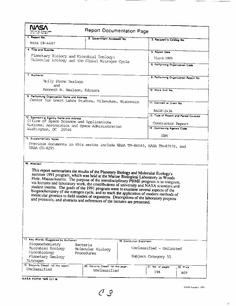
Report Documentation Page
I. RIDOrt NO, 2, Government Acces.i,)n No, 3. Reclpbenl's Cat,1)log No.
NASA CR-4497
5. Report Oate
March 1993
4, Tale and Sub0tke
Planetary Biology and _crobial Ecology:
_.blecular Ecology and the Global Nitrogen Cycle
7 Author(s)
_blly Stone Nealson
and
Kenneth H. Nealson, Editors
9. Performing Orgamzauon Narr_ and Address
Center for Great Lakes Studies, Milwaukee, Wisconsin
12 Sponsoring Agency Name and Addre_
Office of Space Science and Applications
National Aeronautics and Space Administration
Washington, 13(i 20546
6. Psdormmg O_'gen_zat.m"_ Code
8. Perform,ng O,gan,zat_on Repofl No
10. Work Unit No.
11, Contract or Grant NO.
NAGW-2436
13. Type of Report ,_nd Per,Od Covered
Contractor Report
•14. Sponsorin_ Agency Co¢_
SE_
15 Supp(ementa_ Notes
Previous documents
NASA CR-4295
in this series include NASA TM-86043, NASA TM-87570, and
16. Abstract
This report summarizes the results of the Planetary Biology and Molecular Ecology'ssummer 1991 program, which was held at the Marine Biological Laboratory in WoodsHole, Massachusetts. The purpose of the interdisciplinary PBME program is to integrate,via lectures and laboratory work, the contributions of university and NASA scientists andstudent interns. The goals of the 1991 program were to examine several aspects of thebiogeochemistry of the nitrogen cycle, and to teach the application of modem methods ofmolecular genetics to field studies of organisms. Descriptions of the laboratory projectsand protocols, and abstracts and references of the lectures are presented.
17. Key Words (Suggested by Authorls)l 18 Distr,but,on Statement
Biogeochemi stry BacteriaUnclassified - Unlimited
Microbial Ecology Molecular Biology
t.iicrobiology Procedures Subject Category 55Planetary Geology
Nitrogen
19 SecuriTy Classif (of ih_s reporlt 20. Secu,,ly Classd. (of th,s paget ] 21 No of pages
Unclassified Unclassified I 196
22 P.ce
A09
NASA FORM 16.26 OCT _6
N ASA-Langh'y. I993

"T
Z
J
T
=
%
s
&
uJnleN lo N oG (tenuev_ leiSO d8gL uo!;3es) alqeJaA!lapuR JI :N3Z£V_NISOd
tg9 ON it_Uqd
VSVN
GtVd $339 R qgviSOd
3iVH SSVqO-HiHn04 qvtOBdS
VSVN
ss_qo HJ.Un09 00£$ 'esfl ele^pd Jol ,_ll_Ue=lllleulsnl_ IB!o!I40
9_£0_ OO uol6u!qse_
lip epoouo!leJls!u!uuPV coeds
pue soBneuoJev leuoBeN
Related Documents


![REVISED Terrestrial Ecology Agenda 8:30 AM Welcome – Logistics, Agenda [Peter Griffith, NASA GSFC/Sigma; Diane Wickland, NASA HQ] 8:40 AM Terrestrial Ecology.](https://static.cupdf.com/doc/110x72/56649d605503460f94a41d22/revised-terrestrial-ecology-agenda-830-am-welcome-logistics-agenda-peter.jpg)