Molecular Dynamics: an outlook Giovanni Ciccotti IAC “Mauro Picone” - CNR Roma and Università di Roma “La Sapienza” and School of Physics UCD Dublin

Welcome message from author
This document is posted to help you gain knowledge. Please leave a comment to let me know what you think about it! Share it to your friends and learn new things together.
Transcript

Molecular Dynamics: an outlook
Giovanni Ciccotti IAC “Mauro Picone” - CNR Roma
and
Università di Roma “La Sapienza” and
School of Physics UCD Dublin

Molecular Dynamics: an outlook
• Where from MD simulations?
• What is MD?
• MD(or, for that, MC) as Equilibrium Statistical Mechanics
• A challenging case: Rare Events and Free Energies
• MD as Non-Equilibrium StatMech ( ➔ multiscale etc)
• Hydrodynamics from an atomistic viewpoint
if time permits
• Holonomic constraints and Blue Moon
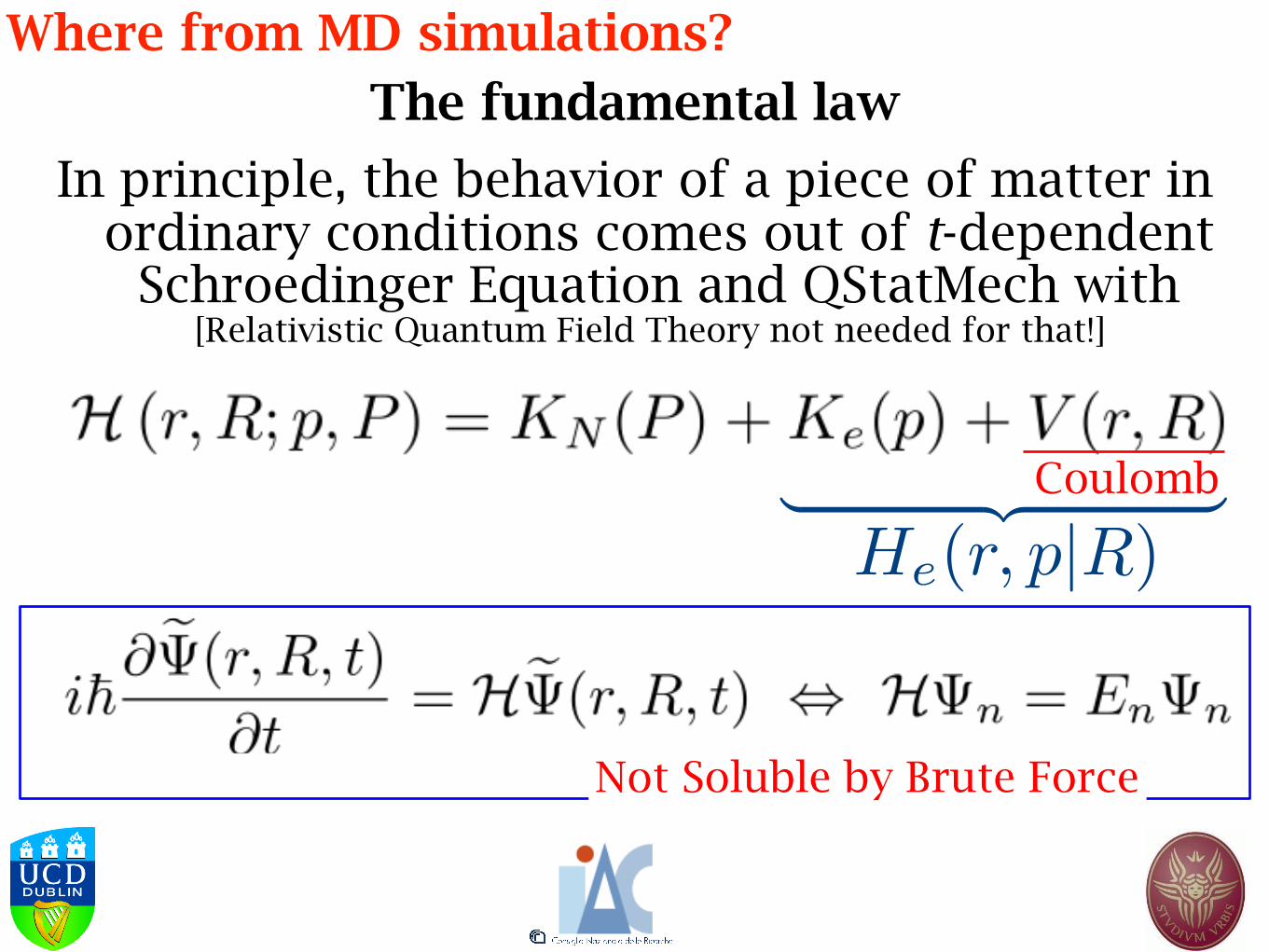
The fundamental lawWhere from MD simulations?
In principle, the behavior of a piece of matter in ordinary conditions comes out of t-dependent
Schroedinger Equation and QStatMech with
Coulomb
[Relativistic Quantum Field Theory not needed for that!]
| {z }
Not Soluble by Brute Force
He(r, p|R)
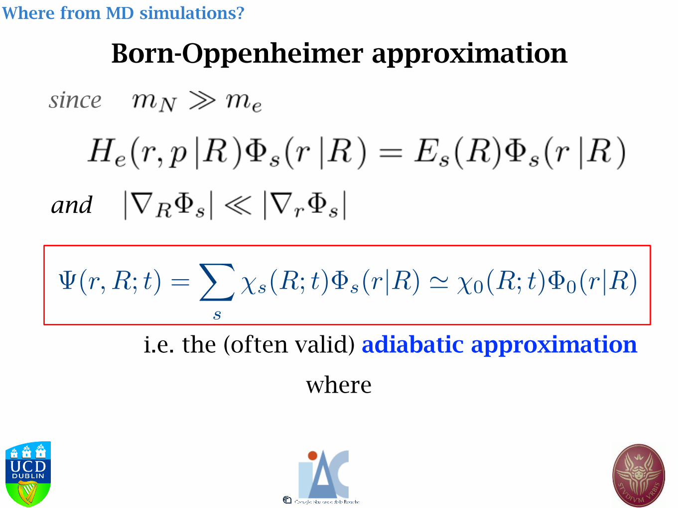
Where from MD simulations?
Born-Oppenheimer approximation
since
i.e. the (often valid) adiabatic approximation
and
(r,R; t) =X
s
�s(R; t)�s(r|R) ' �0(R; t)�0(r|R)
where

the dynamics of the nuclei, apparently independent from the electrons, is driven by E0(R) as interaction potential
(a mean field, modelizable, no more Coulomb!)
Where from MD simulations?
�0(R; t) is given by
ı~ @
@t�0(R; t) = HN (R,P )�0(R; t)
⌘ [KN (P ) + E0(R)]�0(R; t)
the strict adiabatic approximation (no electronic jumps allowed)

Dynamics, no more quantum, is Newton:
rTkm
h
BN
arinternucle<<=Λ
Where from MD simulations?
nuclei are heavy enough
temperature is high enough so that {when
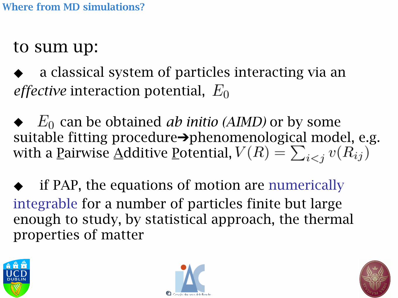
to sum up:
⬥ a classical system of particles interacting via an effective interaction potential,
⬥ can be obtained ab initio (AIMD) or by some suitable fitting procedure➔phenomenological model, e.g. with a Pairwise Additive Potential,
⬥ if PAP, the equations of motion are numerically integrable for a number of particles finite but large enough to study, by statistical approach, the thermal properties of matter
Where from MD simulations?
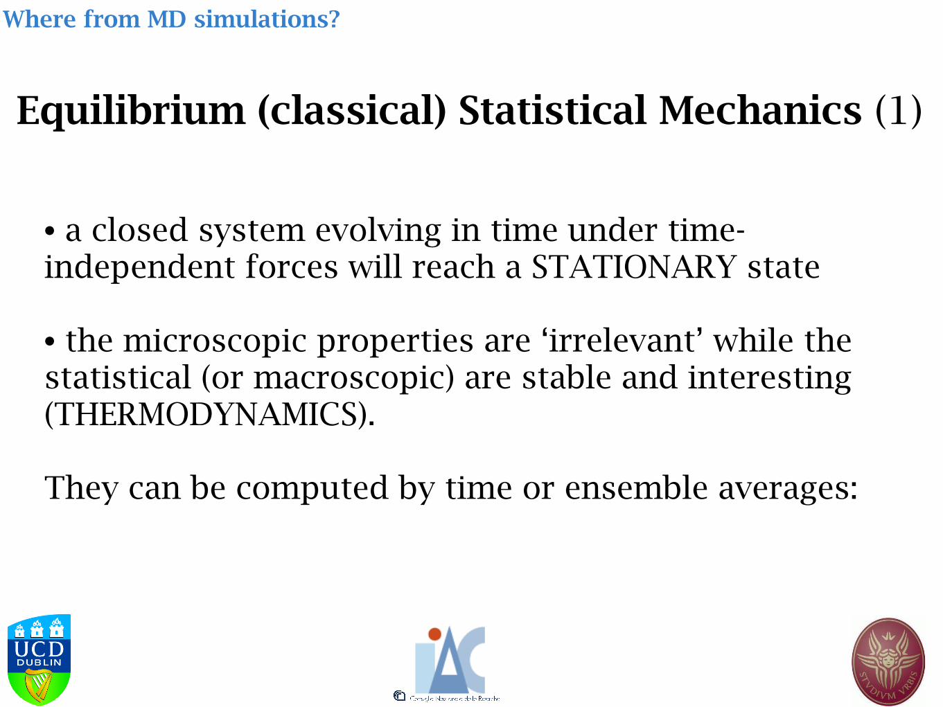
Equilibrium (classical) Statistical Mechanics (1)
• a closed system evolving in time under time-independent forces will reach a STATIONARY state
• the microscopic properties are ‘irrelevant’ while the statistical (or macroscopic) are stable and interesting (THERMODYNAMICS).
They can be computed by time or ensemble averages:
Where from MD simulations?
Where from MD simulations?
hO(R,P )i
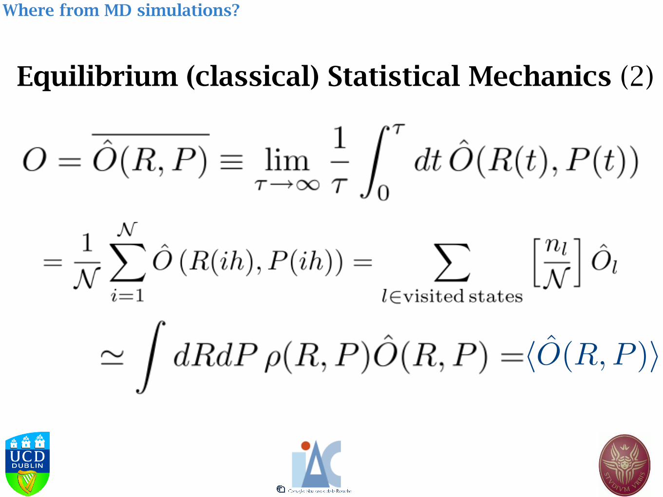
Equilibrium (classical) Statistical Mechanics (2)

ObservableBoltzmann
νl probability of state l
Ensemble or probability density
⬥ properties coming from an observable ➔ mechanical (e.g., pressure)
⬥ properties coming from or , i.e. probability ➔ thermal (e.g., free energy)
Gibbs
Where from MD simulations?
Equilibrium (classical) Statistical Mechanics (3)
⇢nl

(BO originated) Classical Stat. Mech. Model
• atoms / molecules point particles (p.p.), / connected sets of p.p., Interactions between p.p.,
• Boundary Conditions (compulsory, no BC’s no equilibrium)
• Initial Conditions (necessary to start although irrelevant for macroscopic behavior. However, they can be a headache!)
• Evolution laws: Newton equations and Laplace deterministic dream,
What is MD?
{r(t; r0, p0), p(t; r0, p0)}t2(0,⌧!1)
Theoretically:

Computationally:
What is MD?
simple pairwise additive ; short range (MIC)
extensions: ➔ long range (Coulomb) by Ewald sums
Extensions: ➔ n-body potentials but glue potential
Extensions: ➔ stiff intramolecular potentials: Constraints: : SHAKE Multiple Time-Step (Martyna,Tuckerman, Berne) : RESPA
:
for thermodynamic limit: min(S/V) effect
N ⇠ 32÷ 10
6(10
9), n =
N
VBoundary Conditions : Periodic (PBC)
Initial Conditions: positions, regular lattice; velocities, maxwellian
Integration Algorithms: robust, time reversible, symplectic e.g. velocity Verlet Various ensembles (thermostats, barostats … ): extended variables simulations (Andersen, Nosé, Hoover,…
How?
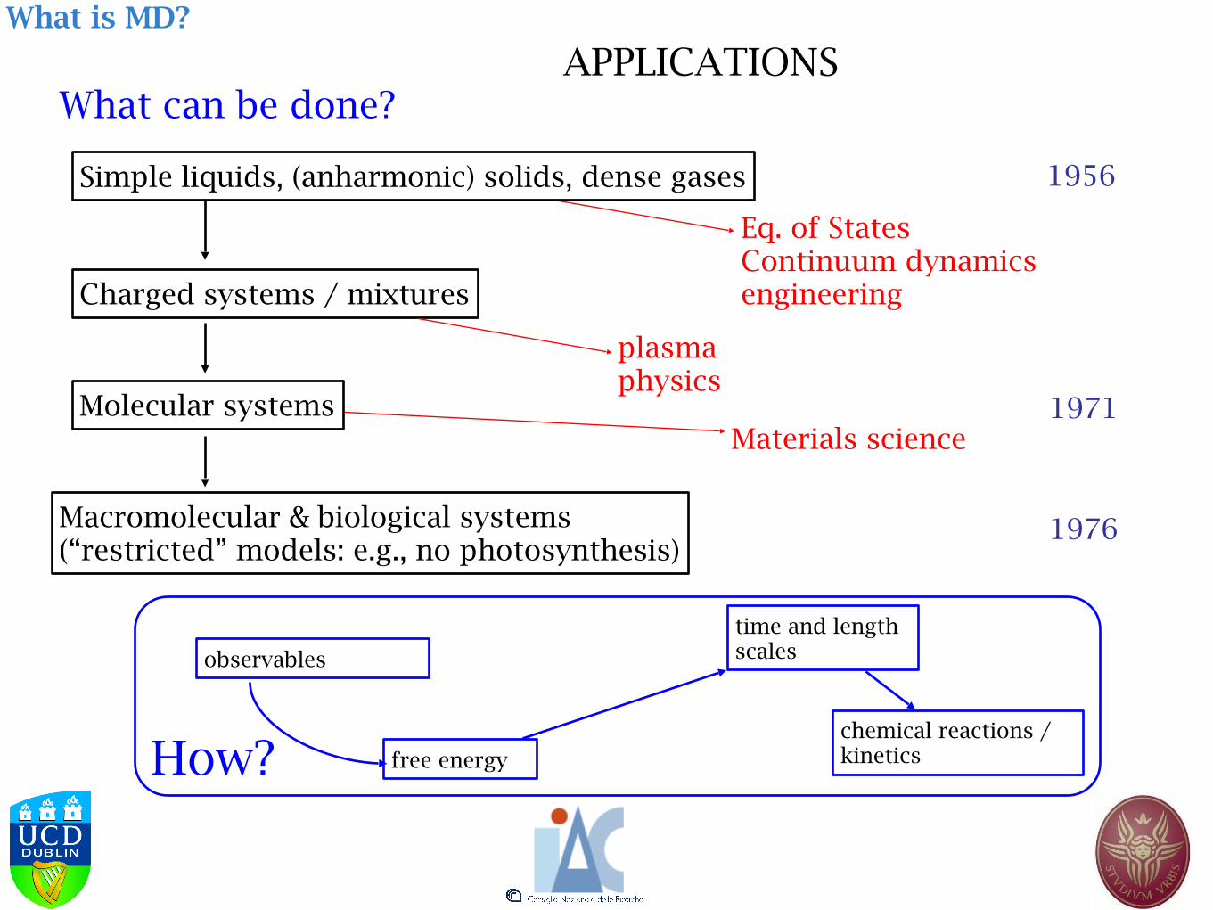
What can be done?
Simple liquids, (anharmonic) solids, dense gases
Charged systems / mixtures
Molecular systems
Macromolecular & biological systems (“restricted” models: e.g., no photosynthesis)
1956
1971
1976
Eq. of States Continuum dynamics engineering
plasma physics
Materials science
observables
free energy
time and length scales
chemical reactions / kinetics
What is MD?
APPLICATIONS

Probabilistic interpretation of the thermal properties
• Entropy (Boltzmann)
• Similarly in general ensembles
where is the probability density function of the given ensemble
Free energies for rare events

Mechanical vs thermal properties
Mechanical property
Thermal property
Free energies for rare events

Free energy of collective variables
• Given a collective variable (i.e. a function of the configuration space) , the free energy associated with its probability density function is
Free energies for rare events
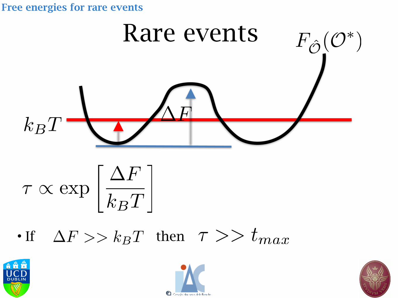
Rare events
• If then
Free energies for rare events
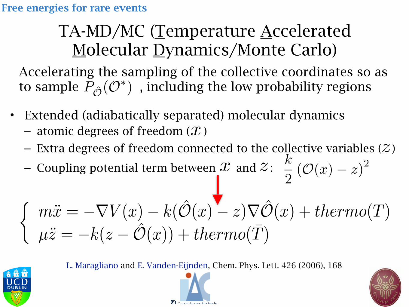
TA-MD/MC (Temperature Accelerated Molecular Dynamics/Monte Carlo)
Accelerating the sampling of the collective coordinates so as to sample , including the low probability regions
Free energies for rare events
• Extended (adiabatically separated) molecular dynamics – atomic degrees of freedom ( )
– Extra degrees of freedom connected to the collective variables ( )
– Coupling potential term between and :
L. Maragliano and E. Vanden-Eijnden, Chem. Phys. Lett. 426 (2006), 168

TAMD: adiabaticity
• are much faster than moves according to the effective force
(we have assumed that, apart for the , the remaining degrees of freedom of the system are ergodic)
Free energies for rare events

TAMD: the strong coupling limit
• Interpretation of the effective force as mean force
Free energies for rare events

TAMD: collective variable at high temperature
Suitable interpolation algorithms (e.g. Single Sweep) can be used to reconstruct from these data the free energy surface
Free energies for rare events

TAMC: the problem of non-analytical Collective Variables
• In TAMD nuclei evolve under the action of:
• TAMD (but also Metadynamics, Adiabatic Dynamics, …) can be used only if the collective variable is an explicit-analytic function of the atomic positions
• In TAMC nuclei are evolved by MC instead than by MD according to the accelerated probability density function while the ’s are still evolved by MD. The adiabaticity conditions are easy to generalise so that we have a more powerful tool
Free energies for rare events

Where is TAMC extension important?
• Classical cases
– Nucleation – Rigorous collective variable to localize vacancies in
solids
• Quantum cases: let the observable be the quantum average then therefore for TAMD, and similar techniques, we need
Free energies for rare events

TAMC: application to the nucleation of a moderately undercooled L-J liquid
Targets • Get the free energy as a
function of the number of atoms of a given crystalline nucleus
• Critical size of the nucleus • Mechanism of growth of
the nucleus (hopefully)
Typical free energy as function of the number of atoms in the crystalline nucleus
Free energies for rare events

Collective variable for nucleation
• Nucleus Size (NS): – Number of atoms in the largest cluster of (i) connected, (ii) crystal-like atoms (i) Two atoms with are connected when their are almost
parallel1
(ii) Crystal-like atoms: atoms with 7 or more connected atoms1
• To identify the largest cluster one has to use methods of graph theory (e.g. the “Deep First search” which we used)
The NS is mathematically well defined but non analytical
1) P. R. ten Wolde, M. J. Ruiz-Montero and D. Frenkel, J. Chem. Phys. 104 (1996) 9932
Free energies for rare events

Results: timeline MD vs TAMC
Free energies for rare events

Results: free energy vs
0 100 200 300 400 500N
0
10
20
30
40
-ln P
(N) N*~ 230
G. Ciccotti and S. Meloni, “Temperature Accelerated Monte Carlo (TAMC): a method for sampling the free energy surface of non-analytical collective coordinates” PCCP, 13, 5952 (2011)
Free energies for rare events

Results: nucleus configurations
3-layers thick cut through a post-critical nucleus of colloids (by 3D imaging1)
1) U. Gasser, E. R. Weeks, A. Schofield, P. N. Pusey, D. A. Weitz, Science 292 (2001), 258
3-layers thick cut through a post-critical nucleus in our simulations
an under-critical nucleus in our simulations
Free energies for rare events

Hydrodynamic limit of
In books, after the derivation of the Navier-Stokes Eq.s (i.e. conservation laws (exact) + constitutive relations & local equilibrium hypothesis (phenomenological and approximate)) we are given
– i.e an explicit form for
Then, is said, multiplying by and taking an “ensemble average”, we get
BUT is a macroscopic quantity, there is no ensemble over which to average. What kind of average is ?
Non-Equilibrium MD (Dynamical-NEMD)
nk(t) = f(k, t) nk(t)n�k(0)
Fk(t) = 1/N << nk(t)n�k(0) >>
nk(t)

Hydrodynamic limit of
The question is: what is the meaning of the macroscopic in Stat. Mech. and within the given approximations? Well,
i.e. is a standard conditional average over a suitable ensemble.
Multiplying by the condition and averaging over its probability distribution we get the : puzzle solved! The question of this talk is: can we compute hydrodynamic fields, included , by some rigorous D-NEMD approach?
Hydrodynamics from Dynamical Non-Equilibrium Molecular Dynamics
nk(t)
nk(t) = hnk (�(t)) |n�k(�) = n�k(0)i
Pn�k (n�k(0))
nk(t)

Relation between microscopic and macroscopic fields
How is defined the microscopic field associated to the macroscopic field ?
is the microscopic property associated to the field,
e.g. : , , …
The macroscopic field is related to the corresponding microscopic field via a suitable average, conditional to the values of a set of scalar/field observables at t=0, ( ) :
Hydrodynamics from Dynamical Non-Equilibrium Molecular Dynamics
~p(~x, t) ! Oi(�) = ~pi
O(~x, t) = hO(~x,�(t)icond
n(~x, t) ! Oi(�) = mi
C(~x,�) = C(~x, t = 0)
ˆ
ˆ ˆ
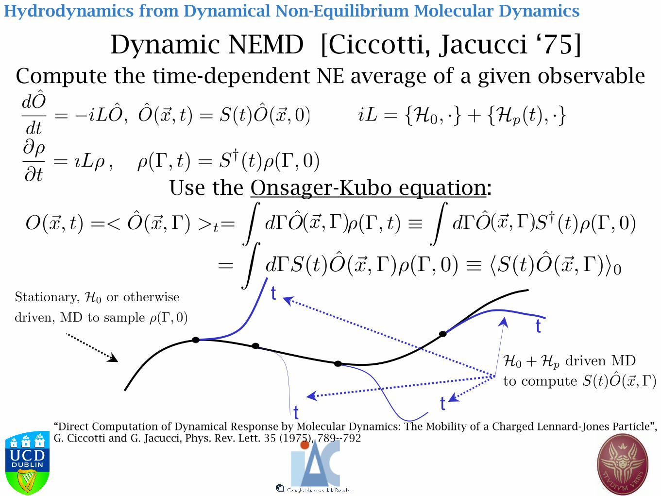
Compute the time-dependent NE average of a given observable
Use the Onsager-Kubo equation:
Dynamic NEMD [Ciccotti, Jacucci ‘75]
t
tt
t
“Direct Computation of Dynamical Response by Molecular Dynamics: The Mobility of a Charged Lennard-Jones Particle”, G. Ciccotti and G. Jacucci, Phys. Rev. Lett. 35 (1975), 789--792
Hydrodynamics from Dynamical Non-Equilibrium Molecular Dynamics
@⇢
@t= ıL⇢ , ⇢(�, t) = S†(t)⇢(�, 0)
=
Zd�S(t)O(~x,�)⇢(�, 0) ⌘ hS(t)O(~x,�)i0
Stationary, H0 or otherwise
driven, MD to sample ⇢(�, 0)
O(~x, t) =< O(~x,�) >t=
Zd�O(~x, t)⇢(�, t) ⌘
Zd�O(~x, t)S†(t)⇢(�, 0)(~x,�) (~x,�)
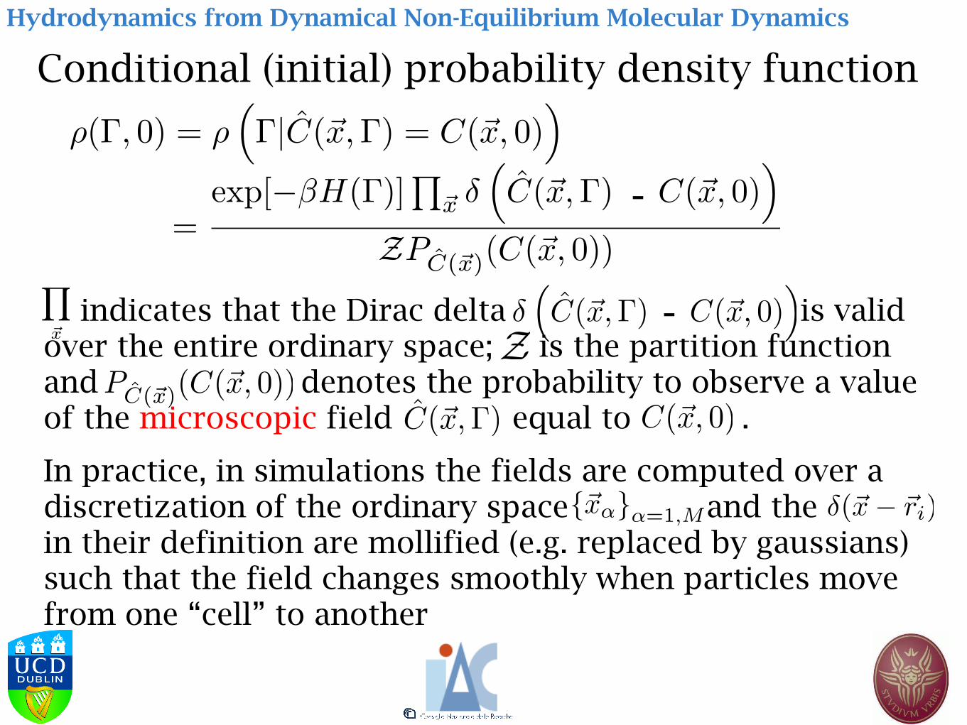
Conditional (initial) probability density function
indicates that the Dirac delta is valid over the entire ordinary space; is the partition function and denotes the probability to observe a value of the microscopic field equal to .
In practice, in simulations the fields are computed over a discretization of the ordinary space and the in their definition are mollified (e.g. replaced by gaussians) such that the field changes smoothly when particles move from one “cell” to another
Hydrodynamics from Dynamical Non-Equilibrium Molecular Dynamics
⇢(�, 0) = ⇢
⇣�|C(~x,�) = C(~x, 0)
⌘
-
-

• The sampling of the conditional ensemble can be performed by restrained MD
where: €
Conditional averages by restrained MD
Hydrodynamics from Dynamical Non-Equilibrium Molecular Dynamics
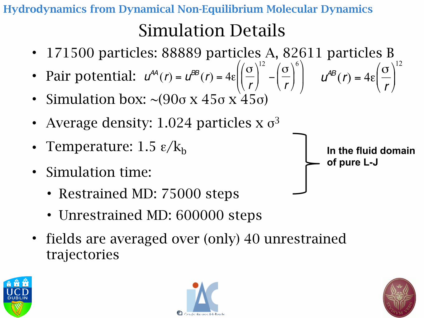
• 171500 particles: 88889 particles A, 82611 particles B
• Pair potential:
• Simulation box: ~(90σ x 45σ x 45σ)
• Average density: 1.024 particles x σ3
• Temperature: 1.5 ε/kb
• Simulation time:
• Restrained MD: 75000 steps
• Unrestrained MD: 600000 steps
• fields are averaged over (only) 40 unrestrained trajectories
€
Simulation Details
€
uAA (r) = uBB (r) = 4εσr
⎛
⎝ ⎜
⎞
⎠ ⎟ 12
−σr
⎛
⎝ ⎜
⎞
⎠ ⎟ 6⎛
⎝ ⎜
⎞
⎠ ⎟
€
uAB (r) = 4εσr
⎛
⎝ ⎜
⎞
⎠ ⎟ 12
In the fluid domain of pure L-J
Hydrodynamics from Dynamical Non-Equilibrium Molecular Dynamics

Hydrodynamic evolution of an interface by restrained- and NE-MD
PBC
"Hydrodynamics from statistical mechanics: combined dynamical-NEMD and conditional sampling to relax an interface between two immiscible liquids.", S. Orlandini, S. Meloni, G. Ciccotti, Phys. Chem. Chem. Phys. 13, 13177 (2011)
Hydrodynamics from Dynamical Non-Equilibrium Molecular Dynamics
�n(~x↵,�) = n
A(~x↵,�)� n
B(~x↵,�) = 0 , ~x↵ 2 S

Hydrodynamics from Dynamical Non-Equilibrium Molecular Dynamics
�n(~x↵, t) = 0

t
t
Hydrodynamics from Dynamical Non-Equilibrium Molecular Dynamics
�n(~x↵, t) = 0
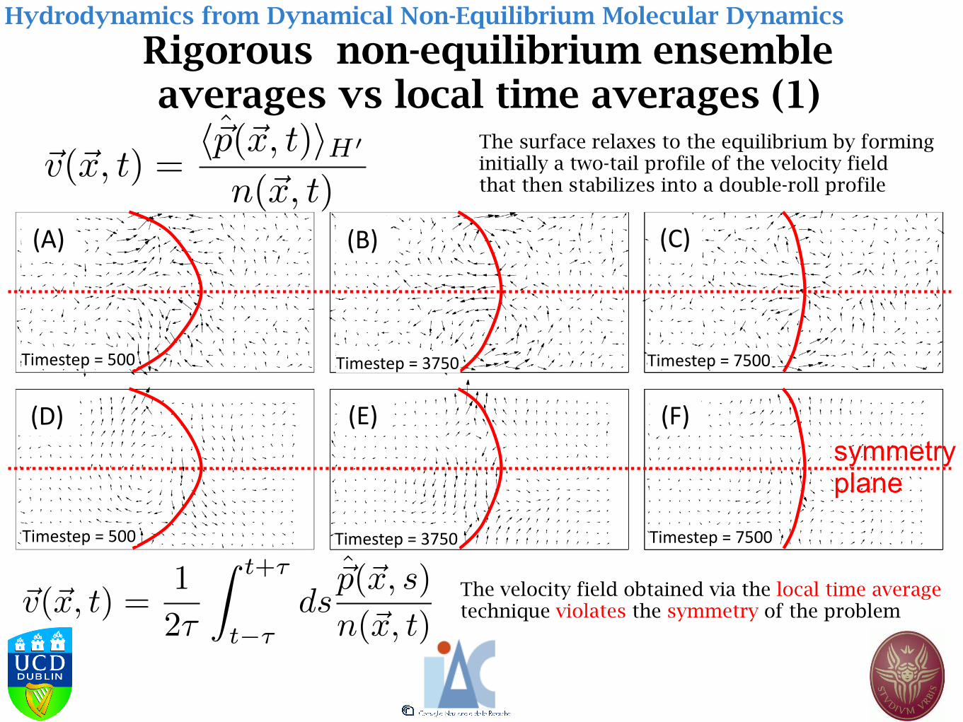
Rigorous non-equilibrium ensemble averages vs local time averages (1)
!"#$
%&'()*(+$,$-..$
!/#$
%&'()*(+$,$01-.$
!2#$
%&'()*(+$,$1-..$
!3#$
%&'()*(+$,$-..$
!4#$
%&'()*(+$,$01-.$
!5#$
%&'()*(+$,$1-..$
Hydrodynamics from Dynamical Non-Equilibrium Molecular Dynamics
symmetry plane
The surface relaxes to the equilibrium by forming initially a two-tail profile of the velocity field that then stabilizes into a double-roll profile
The velocity field obtained via the local time average technique violates the symmetry of the problem
~v(~x, t) =h~p(~x, t)iH0
n(~x, t)
~v(~x, t) =1
2⌧
Z t+⌧
t�⌧ds
~p(~x, s)
n(~x, t)
Conclusions� Molecular Dynamics Simulations (MS) are a regular
chapter of Theoretical Physics BUT they are amenable to real applications both for the analysis of experiments and for engineering
� New algorithms have been, and continue to be, introduced to circumvent practical limitations of the MS, i.e. problems which cannot be solved by brute force. A good example has been TAMD/TAMC
� Also NonEquilibrium situations can be confronted by a proper use of Onsager-Kubo relationship. This opens the way to represent directly transport but also to atomistic simulations (without constitutive hypotheses) of hydrodynamical phenomena.
Molecular Dynamics: an outlook

Dynamical systems with (holonomic) constraints
To keep the trajectories satisfying the constraints
we must have also
# molecules
# atoms in molecule i
plus �k ({r}) = 0 , k = 1, f # constraints
i = 1, N
↵ = 1, ni
e.g. � ({r}) = (ri↵ � ri�)2 � d2i,↵� = 0
{
(� ({r(t)}) = 0 , 8t )( � = r ·rr� ({r(t)}) = 0 , 8t )
Moreover, if the constraint forces do not do work (i.e. conserve energy)
where the intensity of the constraint force has to be determined
r · G ({r}) = 0 , Gi↵ = �fX
k=1
�kri↵�k ⌘ �� ·ri↵�
�
L ({r, r}) = 12
X
i,↵
mi↵ri↵ � U ({r})2

SHAKE (1)
By differentiating two times the constraint relations ’s we find
from which the useless solution of the linear system (✳✳✳)
due to the problem of the algorithmic error, destroying the model.
�
�k = r ·rr�k + (rr) · (rrrr)�k = 0
and from i.e. (✳✳)d
dt
@L@r
� @L@r
= G mr = F� � · (rr�)
(✳)
� = 1m (F� (�rr) · �) ·rr� + (rr ·rrrr)� = 0 (✳✳✳)
� = Z�1 [(F ·rr)� + (rr ·rrrr)�] , Zk` = rr�k ·rr�`

SHAKE (2)
E.g.
where, plugging e.g. (+) in (++) one gets values which satisfy exactly the constraints at timestep (t+h) without increasing the algorithmic error
(++) can be solved by any efficient algorithm. E.g. the Newton-Raphson method
exact at all timesteps will destroy in time the conservation of constraints
(+)
(++)
G(t)
Instead, exploiting the “freedom” to choose the to satisfy the constraints one can write the set of equations
�
�k ({r(t+ h)}) = 0 , k = 1, . . . , f
r(t+ h) = r(t) + hr+ h2
2m [F(t) + G(t)] +O(h3)
�

SMwC (1)
NOW: instead of assuming the constraints satisfied, let us take the constraint functions as f generalized coordinates. THEN
In analytical mechanics, in presence of constraints
The constrained system will be obtained putting back
Statistical Mechanics of systems with constraints in cartesian coordinates
r �! r(q) r : 3N ;q : 3N � f
r = q ·rqr
L0 (r, r) �! L0 (q, q) =) H (q,pq)⇣pq = @L
@q
⌘
and, for Statistical Mechanics
Q =
Zdqdpqe��H(q,pq)
�(r) = 0 , �(r, r) = 0
pu = Mur ! ((q, �) ⌘ u) pr ! (pu ⌘ (pq, p�)) with

SMwC (2)
we have that
corresponds to
Considering that
i.e. to not zero, for , but equal to
and
L(r, r) = K(r)� V(r) = L(u, u) = 12 u
TMu� V 0(u)
� = 0
� = ETpq + Zp� = 0
i.e. u =
✓q�
◆= M�1pu =
✓� EET Z
◆✓pq
p�
◆
pu =
✓pq
p�
◆=
@L0
@u= Mu =
✓A BBT �
◆✓q�
◆
p� � = 0 p� = Z�1ETpq
p� + p� = Z�1�

SMwC (3)
so
Now our result is at hand, since
where since the transformation is canonical and the Jacobian is = 1
Moreover
L0(u, u) ! H0(pu,u)
Hc(pq,q) = H0(pq,p� = Z�1ETpq , q,� = 0)
Q =
Zdqdpqe��Hc =
Zdudpue��H0(pu,u)� (�) � (p� � p�)
=
Zdrdpre��H(pr,r)� (�(r)) �
�Z�1�(r,pr)
�
dudpu = drdpr
%(r,pr) = 1Qe��H(pr,r)� (�(r)) �
�Z�1�(r,pr)
�

ASBM (1)
We assume a metastabi l i ty in conf igurat ional space and the existence of at least one configurational function (a lso often improper ly ca l led a react ion coordinate ) such that its values going from A to B grow monotonically from to and can then be used to characterise the STATE of the system at and between the two metastable states. The system spends the majority of its time in A or B and very little in between. The transitional region has almost zero probability to be visited and MD is unable to sample the full space
Accelerated (but rigorous) Sampling: Blue Moon Ensemble
�A �B > �A
� = �1 � = �2� = �T

ASBM (2)
1. using as a constraint we can sample by MD any chosen region
2. By knowing the probability in presence of a constraint (as shown before) we can demonstrate that (✕) where the second term is virtually impossible to sample while the third is obtained with full statistics.
3. the integral of (✕) [THERMODYNAMICAL INTEGRATION] provides a direct measure of the strength of the metastability
We would l ike to know for a l l possible va lues (probable and improbable) of .
P� (�0)
�0
� ({r})
d lnP⌅(⇠0)
d⇠
0 / hF⇠
0icond
=hcorrF
⇠
0iconstrained
hcorriconstrained
Related Documents