Molecular distributions in gene regulatory dynamics

HAL Id: hal-00651585https://hal.archives-ouvertes.fr/hal-00651585

Submitted on 18 Dec 2014

HAL is a multi-disciplinary open accessarchive for the deposit and dissemination of sci-entific research documents, whether they are pub-lished or not. The documents may come fromteaching and research institutions in France orabroad, or from public or private research centers.

L’archive ouverte pluridisciplinaire HAL, estdestinée au dépôt et à la diffusion de documentsscientifiques de niveau recherche, publiés ou non,émanant des établissements d’enseignement et derecherche français ou étrangers, des laboratoirespublics ou privés.

Molecular distributions in gene regulatory dynamicsMichael C. Mackey, Marta Tyran-Kamińska, Romain yvinec

To cite this version:Michael C. Mackey, Marta Tyran-Kamińska, Romain yvinec. Molecular distributions in generegulatory dynamics. Journal of Theoretical Biology, Elsevier, 2011, 274 (1), pp.84–96.�10.1016/j.jtbi.2011.01.020�. �hal-00651585�

arX

iv:1

009.

5810

v1 [

q-bi

o.M

N]

29 S

ep 2

010

Molecular Distributions in Gene Regulatory Dynamics

Michael C. Mackey

Departments of Physiology, Physics&Mathematics and Centre for Nonlinear Dynamics, McGill University, 3655 Promenade Sir William Osler, Montreal, QC,

CANADA, H3G 1Y6

Marta Tyran-Kaminska

Institute of Mathematics, University of Silesia, Bankowa 14, 40-007 Katowice, POLAND

Romain Yvinec∗

Universite de Lyon CNRS Universite Lyon 1 , Bat Braconnier 43 bd du 11 nov. 1918 F-69622 Villeurbanne Cedex France

Abstract

We show how one may analytically compute the stationary density of the distribution of molecular constituents in populations ofcells in the presence of noise arising from either bursting transcription or translation, or noise in degradation ratesarising from lownumbers of molecules. We have compared our results with an analysis of the same model systems (either inducible or repressibleoperons) in the absence of any stochastic effects, and shown the correspondence between behaviour in thedeterministic system andthe stochastic analogs. We have identified key dimensionless parameters that control the appearance of one or two steadystates inthe deterministic case, or unimodal and bimodal densities in the stochastic systems, and detailed the analytic requirements for theoccurrence of different behaviours. This approach provides, in some situations, an alternative to computationally intensive stochas-tic simulations. Our results indicate that, within the context of the simple models we have examined, bursting and degradation noisecannot be distinguished analytically when present alone.

Keywords: Stochastic modelling, inducible/repressible operon.

1. Introduction

In neurobiology, when it became clear that some of the fluc-tuations seen in whole nerve recording, and later in single cellrecordings, were not simply measurement noise but actual fluc-tuations in the system being studied, researchers very quicklystarted wondering to what extent these fluctuations actuallyplayed a role in the operation of the nervous system.

Much the same pattern of development has occurred in cel-lular and molecular biology as experimental techniques haveallowed investigators to probe temporal behaviour at ever finerlevels, even to the level of individual molecules. Experimental-ists and theoreticians alike who are interested in the regulationof gene networks are increasingly focussed on trying to accessthe role of various types of fluctuations on the operation andfidelity of both simple and complex gene regulatory systems.Recent reviews (Kaern et al., 2005; Raj and van Oudenaarden,2008; Shahrezaei and Swain, 2008b) give an interesting per-spective on some of the issues confronting both experimental-ists and modelers.

∗Corresponding authorEmail addresses:[email protected] (Michael C. Mackey),

[email protected] (Marta Tyran-Kaminska),[email protected] (Romain Yvinec)

Typically, the discussion seems to focus on whether fluc-tuations can be considered as extrinsic to the system underconsideration (Shahrezaei et al., 2008; Ochab-Marcinek, 2008,2010), or whether they are an intrinsic part of the fundamen-tal processes they are affecting (e.g. bursting, see below).The dichotomy is rarely so sharp however, but Elowitz et al.(2002) have used an elegant experimental technique to dis-tinguish between the two, see also Raser and O’Shea (2004),while Swain et al. (2002) and Scott et al. (2006) have laid thegroundwork for a theoretical consideration of this question.One issue that is raised persistently in considerations of therole of fluctuations or noise in the operation of gene regulatorynetworks is whether or not they are “beneficial” (Blake et al.,2006) or “detrimental” (Fraser et al., 2004) to the operation ofthe system under consideration. This is, of course, a questionof definition and not one that we will be further concerned withhere.

Here, we consider in detail the density of the moleculardistributions in generic bacterial operons in the presenceof‘bursting’ (commonly known as intrinsic noise in the bio-logical literature) as well as inherent (extrinsic) noise usingan analytical approach. Our work is motivated by the welldocumented production of mRNA and/or protein in stochas-tic bursts in both prokaryotes and eukaryotes (Blake et al.,2003; Cai et al., 2006; Chubb et al., 2006; Golding et al., 2005;

Preprint submitted to Elsevier September 30, 2010

Raj et al., 2006; Sigal et al., 2006; Yu et al., 2006), and fol-lows other contributions by, for example, Kepler and Elston(2001), Friedman et al. (2006), Bobrowski et al. (2007) andShahrezaei and Swain (2008a).

In Section 2 we develop the concept of the operon and treatsimple models of the classic inducible and repressible operon.Section 4 considers the effects of bursting alone in an ensembleof single cells. Section 5 then examines the situation in whichthere are continuous white noise fluctuations in the dominantspecies degradation rate in the absence of bursting.

2. Generic operons

2.1. The operon concept

The so-called ‘central dogma’ of molecular biology is sim-ple to state in principle, but complicated in its detail. Namelythrough the process oftranscriptionof DNA, messenger RNA(mRNA, M) is produced and, in turn, through the process oftranslation of the mRNA proteins (intermediates,I ) are pro-duced. There is often feedback in the sense that molecules (en-zymes,E) whose production is controlled by these proteins canmodulate the translation and/or transcription processes. In whatfollows we will refer to these molecules aseffectors. We nowconsider both the transcription and translation process inmoredetail.

In the transcription process an amino acid sequence in theDNA is copied by the enzyme RNA polymerase (RNAP) toproduce a complementary copy of the DNA segment encodedin the resulting RNA. Thus this is the first step in the transferof the information encoded in the DNA. The process by whichthis occurs is as follows.

When the DNA is in a double stranded configuration, theRNAP is able to recognize and bind to the promoter region ofthe DNA. (The RNAP/double stranded DNA complex is knownas the closed complex.) Through the action of the RNAP, theDNA is unwound in the vicinity of the RNAP/DNA promotersite, and becomes single stranded. (The RNAP/single strandedDNA is called the open complex.) Once in the single strandedconfiguration, the transcription of the DNA into mRNA com-mences.

In prokaryotes, translation of the newly formed mRNA com-mences with the binding of a ribosome to the mRNA. Thefunction of the ribosome is to ‘read’ the mRNA in triplets ofnucleotide sequences (codons). Then through a complex se-quence of events, initiation and elongation factors bring transferRNA (tRNA) into contact with the ribosome-mRNA complex tomatch the codon in the mRNA to the anti-codon in the tRNA.The elongating peptide chain consists of these linked aminoacids, and it starts folding into its final conformation. This fold-ing continues until the process is complete and the polypeptidechain that results is the mature protein.

The lactose (lac) operon in bacteria is the paradigmatic ex-ample of this concept and this much studied system consists ofthree structural genes namedlacZ, lacY, andlacA. These threegenes contain the code for the ultimate production, throughthetranslation of mRNA, of the intermediatesβ-galactosidase,lac

permease, and thiogalactoside transacetylase respectively. Theenzymeβ-galactosidase is active in the conversion of lactoseinto allolactose and then the conversion of allolactose into glu-cose. Thelac permease is a membrane protein responsible forthe transport of extracellular lactose to the interior of the cell.(Only the transacetylase plays no apparent role in the regula-tion of this system.) The regulatory genelacI, which is part ofa different operon, codes for thelac repressor, which is trans-formed to an inactive form when bound with allolactose, so inthis system allolactose functions as the effector molecule.

2.2. The transcription rate function

In this section we examine the molecular dynamics of boththe classical inducible and repressible operon to derive expres-sions for the dependence of the transcription rate on effectorlevels. (When the transcription rate is constant and indepen-dent of the effector levels we will refer to this as the no controlsituation.)

2.2.1. Inducible regulationFor a typical inducible regulatory situation (such as thelac

operon), in thepresenceof the effector molecule the repressoris inactive (is unable to bind to the operator region precedingthe structural genes), and thus DNA transcription can proceed.Let R denote the repressor,E the effector molecule, andO theoperator. The effector is known to bind with the active formRof the repressor. We assume that this reaction is of the form

R+ nEK1⇋ REn K1 =

REn

R · En, (1)

wheren is the effective number of molecules of effector re-quired to inactivate the repressorR. Furthermore, the operatorO and repressorR are assumed to interact according to

O+ RK2⇋ OR K2 =

ORO · R

.

Let the total operator beOtot:

Otot = O+OR= O+ K2O · R= O(1+ K2R),

and the total level of repressor beRtot:

Rtot = R+ K1R · En + K2O · R.

The fraction of operators not bound by repressor (and thereforefree to synthesize mRNA) is given by

f (E) =O

Otot=

11+ K2R

.

If the amount of repressorR bound to the operatorO is small

Rtot ≃ R+ K1R · En = R(1+ K1En)

so

R=Rtot

1+ K1En,

2

and consequently

f (E) =1+ K1En

1+ K2Rtot + K1En=

1+ K1En

K + K1En, (2)

whereK = 1+ K2Rtot. There will be maximal repression whenE = 0 but even then there will still be a basal level of mRNAproduction proportional toK−1 (which we call the fractionalleakage).

If the maximal DNA transcription rate is ¯ϕm (in units of in-verse time) then, under the assumption that the rate of transcrip-tion ϕ in the entire population is proportional to the fractionfof unbound operators, the variationϕ of the DNA transcriptionrate with the effector level is given byϕ = ϕm f , or

ϕ(E) = ϕm1+ K1En

K + K1En. (3)

2.2.2. Repressible regulationIn the classic example of a repressible system (such as thetrp

operon) in thepresenceof the effector molecule the repressor isactive(able to bind to the operator region), and thus block DNAtranscription. We use the same notation as before, but now notethat the effector binds with the inactive formR of the repressorso it becomes active. We assume that this reaction is of the sameform as in Equation 1. The difference now is that the operatorO and repressorRare assumed to interact according to

O+ R · En K2⇋ OREn K2 =

OREn

O · R · En.

The total operator is now given by

Otot = O+OREn = O+ K2O · R · En = O(1+ K2R · En),

so the fraction of operators not bound by repressor is given by

f (E) =O

Otot=

11+ K2R · En

.

Again assuming that the amount of repressorR bound to theoperatorO is small we have

f (E) =1+ K1En

1+ (K1 + K2Rtot)En=

1+ K1En

1+ KEn,

whereK = K1 + K2Rtot. Now there will be maximal repressionwhenE is large, but even at maximal repression there will stillbe a basal level of mRNA production proportional toK1K−1 <

1. The variation of the DNA transcription rate with effectorlevel is given byϕ = ϕm f or

ϕ(E) = ϕm1+ K1En

1+ KEn. (4)

Both (3) and (4) are special cases of the function

ϕ(E) = ϕm1+ K1En

A+ BEn= ϕm f (E). (5)

whereA, B ≥ 0 are given in Table 1.

parameter inducible repressible

A K = 1+ K2Rtot 1

B K1 K = K1 + K2Rtot

BA

K1

KK

Λ = A K 1

∆ = BK−11 1 KK−1

1

θ =κd

n∆

(

1− ∆Λ

)

κd

n· K − 1

K> 0

κd

n· K1 − K

K< 0

Table 1: Definitions of the parametersA, B,Λ,∆ andθ. See the text and Section2.2 for more detail.

2.3. Deterministic operon dynamics in a population of cells

The reader may wish to consult Polynikis et al. (2009) for aninteresting survey of techniques applicable to this approach.

We first consider a large population of cells, each of whichcontains one copy of a particular operon, and let (M, I ,E) de-note mRNA, intermediate protein, and effector levels respec-tively in the population. Then for a generic operon with a max-imal level of transcriptionbd (in concentration units), we havedynamics described by the system (Griffith, 1968a,b; Othmer,1976; Selgrade, 1979)

dMdt= bdϕm f (E) − γM M, (6)

dIdt= βI M − γI I , (7)

dEdt= βEI − γEE. (8)

Here we assume that the rate of mRNA production is propor-tional to the fraction of time the operator region is active,andthat the rates of intermediate and enzyme production are simplyproportional to the amount of mRNA and intermediate respec-tively. All three of the components (M, I ,E) are subject to ran-dom loss. The functionf is calculated in the previous section.

It will greatly simplify matters to rewrite Equations 6-8 bydefining dimensionless concentrations. To this end we firstrewrite Equation 5 in the form

ϕ(e) = ϕm f (e), (9)

whereϕm (dimensionless) is defined by

ϕm =ϕmβEβI

γMγEγIand f (e) =

1+ en

Λ + ∆en, (10)

Λ and∆ are defined in Table 1, and we have defined a dimen-sionless effector concentration (e) through

E = ηe with η =1

n√

K1.

3

Further defining dimensionless intermediate (i) and mRNAconcentrations (m) through

I = iηγE

βEand M = mη

γEγI

βEβI,

Equations 6-8 can be written in the equivalent form

dmdt= γM[κd f (e) −m],

didt= γI (m− i),

dedt= γE(i − e),

where

κd = bdϕm and bd =bd

η(11)

are dimensionless constants.For notational simplicity, henceforth we denote dimension-

less concentrations by (m, i, e) = (x1, x2, x3), and subscripts(M, I ,E) = (1, 2, 3). Thus we have

dx1

dt= γ1[κd f (x3) − x1], (12)

dx2

dt= γ2(x1 − x2), (13)

dx3

dt= γ3(x2 − x3). (14)

In each equation,γi for i = 1, 2, 3 denotes a net loss rate (unitsof inverse time), and thus Equations 12-14 are not in dimen-sionless form.

The dynamics of this classic operon model can be fully ana-lyzed. LetX = (x1, x2, x3) and denote bySt(X) the flow gener-ated by the system (12)-(14). For both inducible and repressibleoperons, for all initial conditionsX0 = (x0

1, x02, x

03) ∈ R+3 the flow

St(X0) ∈ R+3 for t > 0.Steady states of the system (12)-(14) are in a one to one cor-

respondence with solutions of the equation

xκd= f (x) (15)

and for each solutionx∗ of Equation 15 there is a steady stateX∗ = (x∗1, x

∗2, x∗3) of (12)-(14) given by

x∗1 = x∗2 = x∗3 = x∗.

Whether there is a single steady stateX∗ or there are multiplesteady states will depend on whether we are considering a re-pressible or inducible operon.

2.3.1. No control

In this case,f (x) ≡ 1, and there is a single steady statex∗ =κd that is globally asymptotically stable.

0 1 2 3 4 5 6 70

0.1

0.2

0.3

0.4

0.5

0.6

0.7

0.8

0.9

1

1.1

x

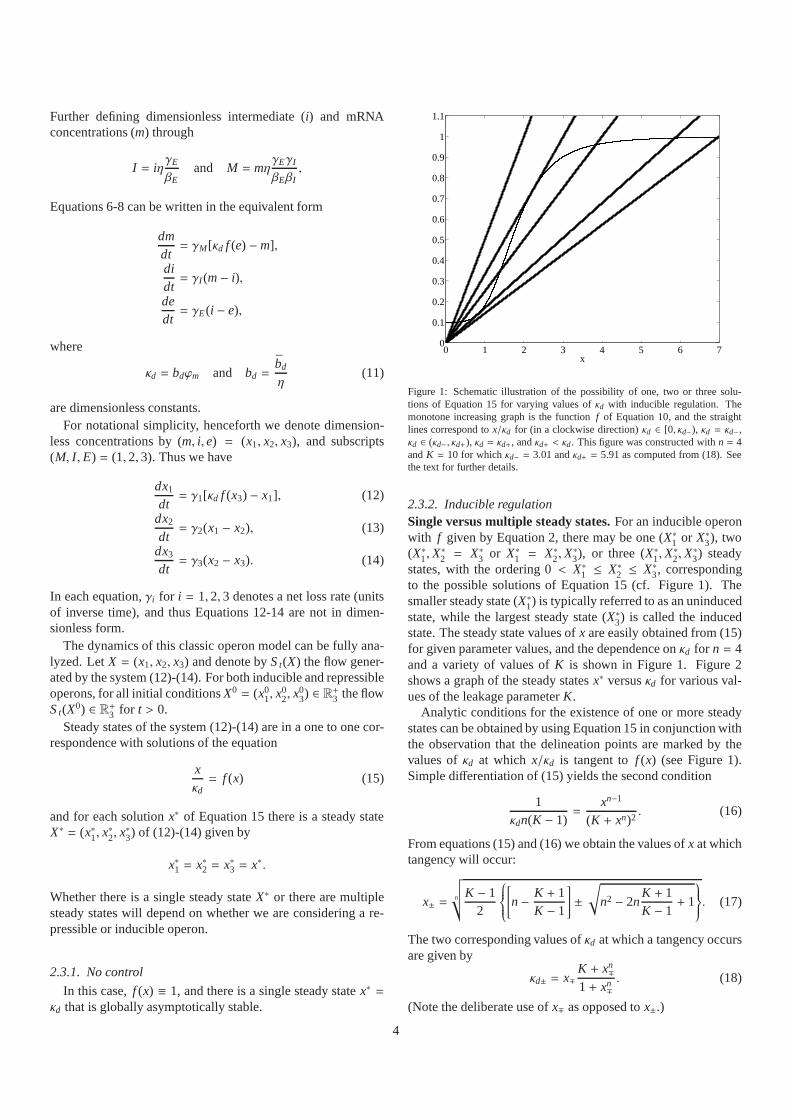
Figure 1: Schematic illustration of the possibility of one,two or three solu-tions of Equation 15 for varying values ofκd with inducible regulation. Themonotone increasing graph is the functionf of Equation 10, and the straightlines correspond tox/κd for (in a clockwise direction)κd ∈ [0, κd−), κd = κd−,κd ∈ (κd−, κd+), κd = κd+, andκd+ < κd. This figure was constructed withn = 4andK = 10 for whichκd− = 3.01 andκd+ = 5.91 as computed from (18). Seethe text for further details.

2.3.2. Inducible regulationSingle versus multiple steady states.For an inducible operonwith f given by Equation 2, there may be one (X∗1 or X∗3), two(X∗1,X

∗2 = X∗3 or X∗1 = X∗2,X

∗3), or three (X∗1,X

∗2,X

∗3) steady

states, with the ordering 0< X∗1 ≤ X∗2 ≤ X∗3, correspondingto the possible solutions of Equation 15 (cf. Figure 1). Thesmaller steady state (X∗1) is typically referred to as an uninducedstate, while the largest steady state (X∗3) is called the inducedstate. The steady state values ofx are easily obtained from (15)for given parameter values, and the dependence onκd for n = 4and a variety of values ofK is shown in Figure 1. Figure 2shows a graph of the steady statesx∗ versusκd for various val-ues of the leakage parameterK.

Analytic conditions for the existence of one or more steadystates can be obtained by using Equation 15 in conjunction withthe observation that the delineation points are marked by thevalues ofκd at which x/κd is tangent tof (x) (see Figure 1).Simple differentiation of (15) yields the second condition

1κdn(K − 1)

=xn−1

(K + xn)2. (16)

From equations (15) and (16) we obtain the values ofx at whichtangency will occur:

x± =n

√

√

K − 12

[

n− K + 1K − 1

]

±√

n2 − 2nK + 1K − 1

+ 1

. (17)

The two corresponding values ofκd at which a tangency occursare given by

κd± = x∓K + xn

∓1+ xn

∓. (18)

(Note the deliberate use ofx∓ as opposed tox±.)

4

1 2 3 4 5 6 7 8 9 10

1

2

3

4

0.5

κd

x*

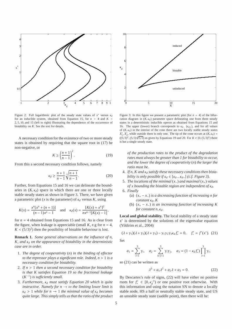
Figure 2: Full logarithmic plot of the steady state values ofx∗ versusκdfor an inducible system, obtained from Equation 15, forn = 4 and K =

2, 5, 10, and 15 (left to right) illustrating the dependence of the occurrence ofbistability onK. See the text for details.

A necessary condition for the existence of two or more steadystates is obtained by requiring that the square root in (17) benon-negative, or

K ≥(

n+ 1n− 1

)2

. (19)

From this a second necessary condition follows, namely

κd ≥n+ 1n− 1

n

√

n+ 1n− 1

. (20)

Further, from Equations 15 and 16 we can delineate the bound-aries in (K, κd) space in which there are one or three locallystable steady states as shown in Figure 3. There, we have givena parametric plot (x is the parameter) ofκd versusK, using

K(x) =xn[xn + (n+ 1)](n− 1)xn − 1

and κd(x) =[K(x) + xn]2

nxn−1[K(x) − 1],

for n = 4 obtained from Equations 15 and 16. As is clear fromthe figure, when leakage is appreciable (smallK, e.g forn = 4,K < (5/3)2) then the possibility of bistable behaviour is lost.

Remark 1. Some general observations on the influence of n,K, andκd on the appearance of bistability in the deterministiccase are in order.

1. The degree of cooperativity(n) in the binding of effectorto the repressor plays a significant role. Indeed, n> 1 is anecessary condition for bistability.

2. If n > 1 then a second necessary condition for bistabilityis that K satisfies Equation 19 so the fractional leakage(K−1) is sufficiently small.

3. Furthermore,κd must satisfy Equation 20 which is quiteinstructive. Namely for n→ ∞ the limiting lower limit isκd > 1 while for n→ 1 the minimal value ofκd becomesquite large. This simply tells us that the ratio of the product

0 5 10 15 200

2

4

6

8

10

K

κd

uninduced

bistable

induced

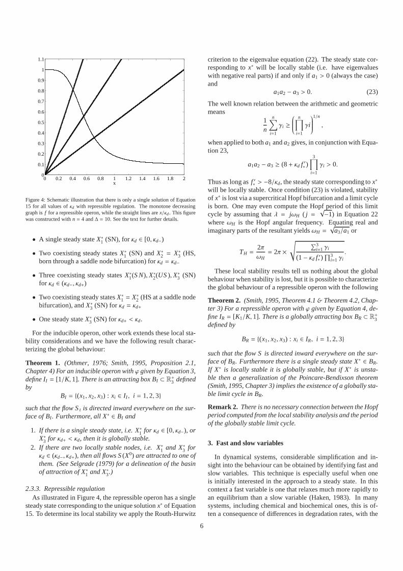
Figure 3: In this figure we present a parametric plot (forn = 4) of the bifur-cation diagram in (K, κd) parameter space delineating one from three steadystates in a deterministic inducible operon as obtained fromEquations 15 and16. The upper (lower) branch corresponds toκd− (κd+), and for all valuesof (K, κd) in the interior of the cone there are two locally stable steady statesX∗1,X

∗3, while outside there is only one. The tip of the cone occurs at(K, κd) =

((5/3)2, (5/3) 4√5/3) as given by Equations 19 and 20. ForK ∈ [0, (5/3)2) thereis but a single steady state.

of the production rates to the product of the degradationrates must always be greater than 1 for bistability to occur,and the lower the degree of cooperativity(n) the larger theratio must be.

4. If n, K andκd satisfy these necessary conditions then bista-bility is only possible ifκd ∈ [κd−, κd+] (c.f. Figure 3).

5. The locations of the minimal(x−) and maximal(x+) valuesof x bounding the bistable region are independent ofκd.

6. Finally(a) (x+ − x−) is a decreasing function of increasing n for

constantκd,K(b) (x+ − x−) is an increasing function of increasing K

for constant n, κd.

Local and global stability. The local stability of a steady statex∗ is determined by the solutions of the eigenvalue equation(Yildirim et al., 2004)

(λ+ γ1)(λ+ γ2)(λ+ γ3)− γ1γ2γ3κd f ′∗ = 0, f ′∗ = f ′(x∗). (21)

Set

a1 =

3∑

i=1

γi , a2 =

3∑

i, j=1

γiγ j , a3 = (1− κd f ′∗ )3

∏

i=1

γi ,

so (21) can be written as

λ3 + a1λ2 + a2λ + a3 = 0. (22)

By Descartes’s rule of signs, (22) will have either no positiveroots for f ′∗ ∈ [0, κ−1

d ) or one positive root otherwise. Withthis information and using the notation SN to denote a locallystable node, HS a half or neutrally stable steady state, and USan unstable steady state (saddle point), then there will be:

5

0 0.2 0.4 0.6 0.8 1 1.2 1.4 1.6 1.8 20

0.1

0.2

0.3

0.4

0.5

0.6

0.7

0.8

0.9

1

1.1

x

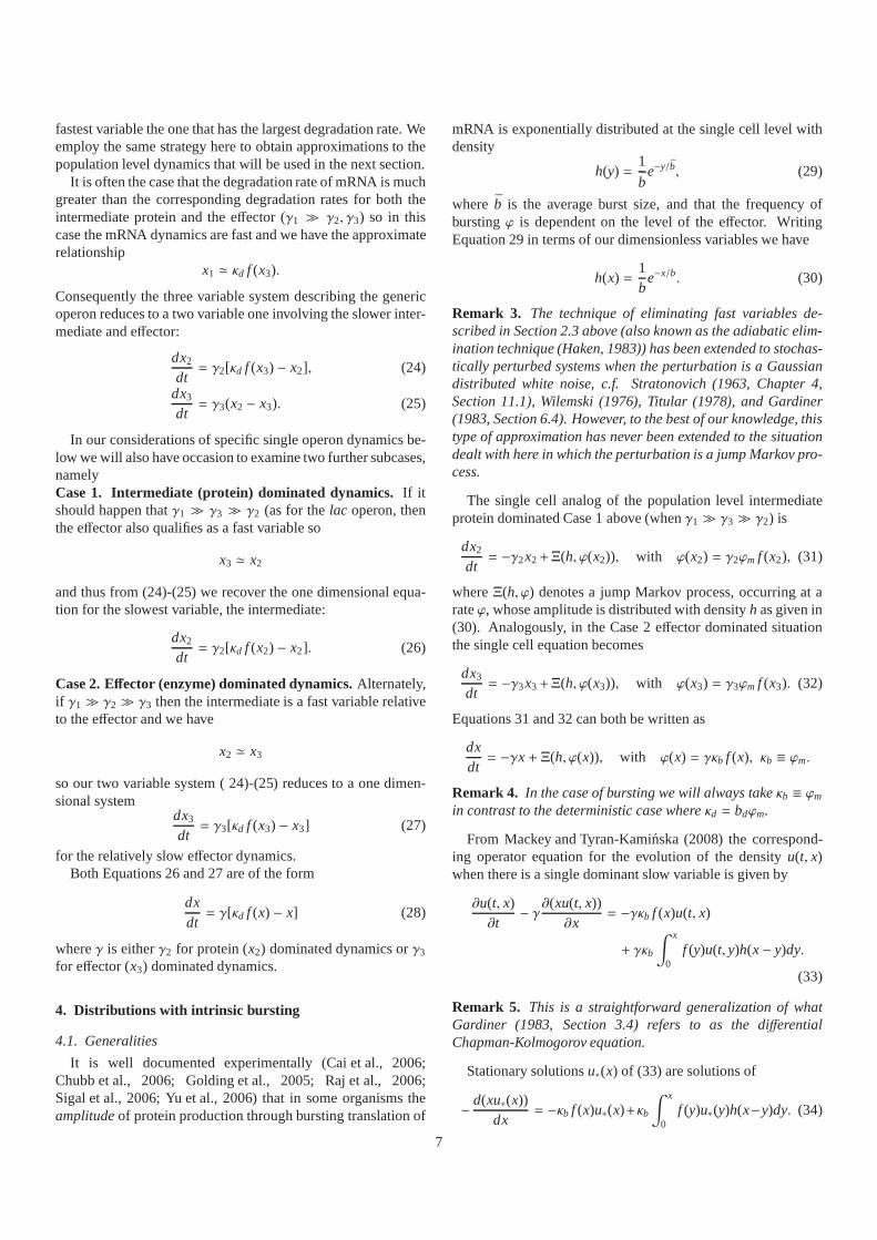
Figure 4: Schematic illustration that there is only a singlesolution of Equation15 for all values ofκd with repressible regulation. The monotone decreasinggraph isf for a repressible operon, while the straight lines arex/κd. This figurewas constructed withn = 4 and∆ = 10. See the text for further details.

• A single steady stateX∗1 (SN), forκd ∈ [0, κd−)

• Two coexisting steady statesX∗1 (SN) andX∗2 = X∗3 (HS,born through a saddle node bifurcation) forκd = κd−

• Three coexisting steady statesX∗1(S N),X∗2(US),X∗3 (SN)for κd ∈ (κd−, κd+)

• Two coexisting steady statesX∗1 = X∗2 (HS at a saddle nodebifurcation), andX∗3 (SN) for κd = κd+

• One steady stateX∗3 (SN) for κd+ < κd.

For the inducible operon, other work extends these local sta-bility considerations and we have the following result charac-terizing the global behaviour:

Theorem 1. (Othmer, 1976; Smith, 1995, Proposition 2.1,Chapter 4) For an inducible operon withϕ given by Equation 3,define II = [1/K, 1]. There is an attracting box BI ⊂ R

+3 defined

byBI = {(x1, x2, x3) : xi ∈ I I , i = 1, 2, 3}

such that the flow St is directed inward everywhere on the sur-face of BI . Furthermore, all X∗ ∈ BI and

1. If there is a single steady state, i.e. X∗1 for κd ∈ [0, κd−), orX∗3 for κd+ < κd, then it is globally stable.

2. If there are two locally stable nodes, i.e. X∗1 and X∗3 forκd ∈ (κd−, κd+), then all flows S(X0) are attracted to one ofthem. (See Selgrade (1979) for a delineation of the basinof attraction of X∗1 and X∗3.)

2.3.3. Repressible regulationAs illustrated in Figure 4, the repressible operon has a single

steady state corresponding to the unique solutionx∗ of Equation15. To determine its local stability we apply the Routh-Hurwitz

criterion to the eigenvalue equation (22). The steady statecor-responding tox∗ will be locally stable (i.e. have eigenvalueswith negative real parts) if and only ifa1 > 0 (always the case)and

a1a2 − a3 > 0. (23)

The well known relation between the arithmetic and geometricmeans

1n

n∑

i=1

γi ≥

n∏

i=1

γi

1/n

,

when applied to botha1 anda2 gives, in conjunction with Equa-tion 23,

a1a2 − a3 ≥ (8+ κd f ′∗ )3

∏

i=1

γi > 0.

Thus as long asf ′∗ > −8/κd, the steady state corresponding tox∗

will be locally stable. Once condition (23) is violated, stabilityof x∗ is lost via a supercritical Hopf bifurcation and a limit cycleis born. One may even compute the Hopf period of this limitcycle by assuming thatλ = jωH ( j =

√−1) in Equation 22

whereωH is the Hopf angular frequency. Equating real andimaginary parts of the resultant yieldsωH =

√a3/a1 or

TH =2πωH= 2π ×

√

∑3i=1 γi

(1− κd f ′∗ )∏3

i=1 γi

.

These local stability results tell us nothing about the globalbehaviour when stability is lost, but it is possible to characterizethe global behaviour of a repressible operon with the following

Theorem 2. (Smith, 1995, Theorem 4.1& Theorem 4.2, Chap-ter 3) For a repressible operon withϕ given by Equation 4, de-fine IR = [K1/K, 1]. There is a globally attracting box BR ⊂ R

+3

defined by

BR = {(x1, x2, x3) : xi ∈ IR, i = 1, 2, 3}

such that the flow S is directed inward everywhere on the sur-face of BR. Furthermore there is a single steady state X∗ ∈ BR.If X∗ is locally stable it is globally stable, but if X∗ is unsta-ble then a generalization of the Poincare-Bendixson theorem(Smith, 1995, Chapter 3) implies the existence of a globallysta-ble limit cycle in BR.

Remark 2. There is no necessary connection between the Hopfperiod computed from the local stability analysis and the periodof the globally stable limit cycle.

3. Fast and slow variables

In dynamical systems, considerable simplification and in-sight into the behaviour can be obtained by identifying fastandslow variables. This technique is especially useful when oneis initially interested in the approach to a steady state. Inthiscontext a fast variable is one that relaxes much more rapidlytoan equilibrium than a slow variable (Haken, 1983). In manysystems, including chemical and biochemical ones, this is of-ten a consequence of differences in degradation rates, with the

6

fastest variable the one that has the largest degradation rate. Weemploy the same strategy here to obtain approximations to thepopulation level dynamics that will be used in the next section.

It is often the case that the degradation rate of mRNA is muchgreater than the corresponding degradation rates for both theintermediate protein and the effector (γ1 ≫ γ2, γ3) so in thiscase the mRNA dynamics are fast and we have the approximaterelationship

x1 ≃ κd f (x3).

Consequently the three variable system describing the genericoperon reduces to a two variable one involving the slower inter-mediate and effector:

dx2

dt= γ2[κd f (x3) − x2], (24)

dx3

dt= γ3(x2 − x3). (25)

In our considerations of specific single operon dynamics be-low we will also have occasion to examine two further subcases,namelyCase 1. Intermediate (protein) dominated dynamics.If itshould happen thatγ1 ≫ γ3 ≫ γ2 (as for thelac operon, thenthe effector also qualifies as a fast variable so

x3 ≃ x2

and thus from (24)-(25) we recover the one dimensional equa-tion for the slowest variable, the intermediate:

dx2

dt= γ2[κd f (x2) − x2]. (26)

Case 2. Effector (enzyme) dominated dynamics.Alternately,if γ1 ≫ γ2 ≫ γ3 then the intermediate is a fast variable relativeto the effector and we have

x2 ≃ x3

so our two variable system ( 24)-(25) reduces to a one dimen-sional system

dx3

dt= γ3[κd f (x3) − x3] (27)

for the relatively slow effector dynamics.Both Equations 26 and 27 are of the form

dxdt= γ[κd f (x) − x] (28)

whereγ is eitherγ2 for protein (x2) dominated dynamics orγ3

for effector (x3) dominated dynamics.

4. Distributions with intrinsic bursting

4.1. Generalities

It is well documented experimentally (Cai et al., 2006;Chubb et al., 2006; Golding et al., 2005; Raj et al., 2006;Sigal et al., 2006; Yu et al., 2006) that in some organisms theamplitudeof protein production through bursting translation of

mRNA is exponentially distributed at the single cell level withdensity

h(y) =1

be−y/b, (29)

where b is the average burst size, and that the frequency ofburstingϕ is dependent on the level of the effector. WritingEquation 29 in terms of our dimensionless variables we have

h(x) =1b

e−x/b. (30)

Remark 3. The technique of eliminating fast variables de-scribed in Section 2.3 above (also known as the adiabatic elim-ination technique (Haken, 1983)) has been extended to stochas-tically perturbed systems when the perturbation is a Gaussiandistributed white noise, c.f. Stratonovich (1963, Chapter4,Section 11.1), Wilemski (1976), Titular (1978), and Gardiner(1983, Section 6.4). However, to the best of our knowledge, thistype of approximation has never been extended to the situationdealt with here in which the perturbation is a jump Markov pro-cess.

The single cell analog of the population level intermediateprotein dominated Case 1 above (whenγ1 ≫ γ3 ≫ γ2) is

dx2

dt= −γ2x2+Ξ(h, ϕ(x2)), with ϕ(x2) = γ2ϕm f (x2), (31)

whereΞ(h, ϕ) denotes a jump Markov process, occurring at arateϕ, whose amplitude is distributed with densityh as given in(30). Analogously, in the Case 2 effector dominated situationthe single cell equation becomes

dx3

dt= −γ3x3+Ξ(h, ϕ(x3)), with ϕ(x3) = γ3ϕm f (x3). (32)

Equations 31 and 32 can both be written as

dxdt= −γx+ Ξ(h, ϕ(x)), with ϕ(x) = γκb f (x), κb ≡ ϕm.

Remark 4. In the case of bursting we will always takeκb ≡ ϕm

in contrast to the deterministic case whereκd = bdϕm.

From Mackey and Tyran-Kaminska (2008) the correspond-ing operator equation for the evolution of the densityu(t, x)when there is a single dominant slow variable is given by

∂u(t, x)∂t

− γ∂(xu(t, x))∂x

= −γκb f (x)u(t, x)

+ γκb

∫ x

0f (y)u(t, y)h(x− y)dy.

(33)

Remark 5. This is a straightforward generalization of whatGardiner (1983, Section 3.4) refers to as the differentialChapman-Kolmogorov equation.

Stationary solutionsu∗(x) of (33) are solutions of

− d(xu∗(x))dx

= −κb f (x)u∗(x)+κb

∫ x

0f (y)u∗(y)h(x−y)dy. (34)

7

If there is a unique stationary density, then the solutionu(t, x) of Equation 33 is said to be asymptotically stable(Lasota and Mackey, 1994) in the sense that

limt→∞

∫ ∞

0|u(t, x) − u∗(x)|dx= 0

for all initial densitiesu(0, x).

Theorem 3. (Mackey and Tyran-Kaminska, 2008, Theorem 7).The unique stationary density of Equation 34, with f given byEquation 9 and h given by (29), is

u∗(x) =Cx

e−x/b exp

[

κb

∫ x f (y)y

dy

]

, (35)

whereC is a normalizing constant such that∫ ∞0

u∗(x)dx = 1.Further, u(t, x) is asymptotically stable.

Remark 6. The stationary density (35) is found by rewritingEquation 34 in the form

dy(x)dx+

y(x)b− κb

f (x)x

y(x) = 0, y(x) ≡ xu∗(x)

using Laplace transforms and solving by quadratures. Notealso that we can represent u∗ as

u∗(x) = C exp∫ x (κb f (y)

y− 1

b− 1

y

)

dy,

whereC is a normalizing constant.

4.2. Distributions in the presence of bursting

4.2.1. Protein distribution in the absence of controlIf the burst frequencyϕ = γκb f is independent of the level

of all of the participating molecular species, then the solutiongiven in Equation 35 is the density of the gamma distribution:

u∗(x) =1

bκbΓ(κb)xκb−1e−x/b,

whereΓ(·) denotes the gamma function. Forκb ∈ (0, 1),u∗(0) =∞ andu∗ is decreasing while forκb > 1, u∗(0) = 0 and there isa maximum atx = b(κb − 1).

4.2.2. Controlled burstingWe next consider the situation in which the burst frequencyϕ is dependent on the level ofx, c.f. Equation 5. This requiresthat we evaluate

κb

∫ x f (y)y

dy=∫ x κb

y

[

1+ yn

Λ + ∆yn

]

dy= ln{

xκbΛ−1

(Λ + ∆xn)θ}

,

whereΛ,∆ are enumerated in Table 1 for both the inducible andrepressible operons treated in Section 2.2 and

θ =κb

n∆

(

1− ∆Λ

)

.

Consequently, the steady state density (35) explicitly becomes

u∗(x) = Ce−x/bxκbΛ−1−1(Λ + ∆xn)θ. (36)

0 1 2 3 4 5 6 70

0.1

0.2

0.3

0.4

0.5

0.6

0.7

0.8

0.9

1

1.1

x

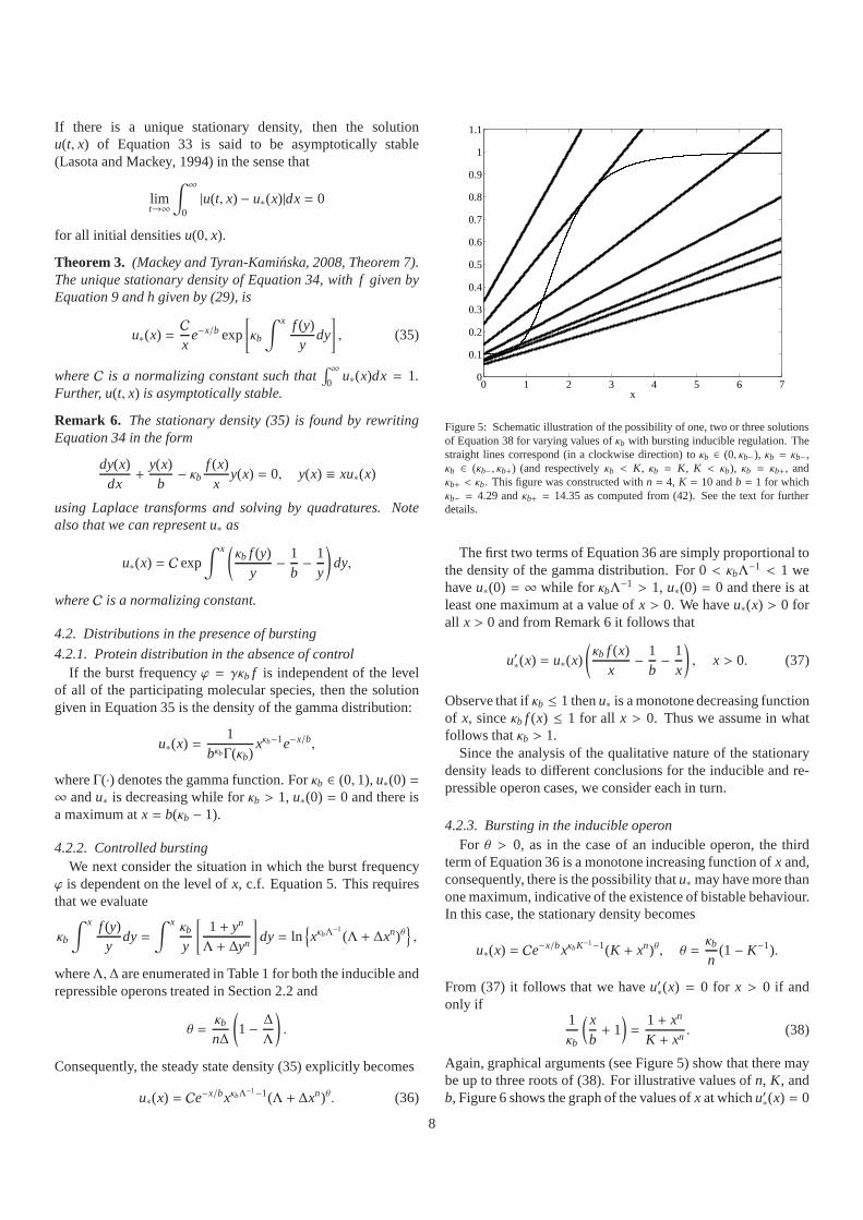
Figure 5: Schematic illustration of the possibility of one,two or three solutionsof Equation 38 for varying values ofκb with bursting inducible regulation. Thestraight lines correspond (in a clockwise direction) toκb ∈ (0, κb−), κb = κb−,κb ∈ (κb−, κb+) (and respectivelyκb < K, κb = K, K < κb), κb = κb+, andκb+ < κb. This figure was constructed withn = 4, K = 10 andb = 1 for whichκb− = 4.29 andκb+ = 14.35 as computed from (42). See the text for furtherdetails.

The first two terms of Equation 36 are simply proportional tothe density of the gamma distribution. For 0< κbΛ−1 < 1 wehaveu∗(0) = ∞ while for κbΛ−1 > 1, u∗(0) = 0 and there is atleast one maximum at a value ofx > 0. We haveu∗(x) > 0 forall x > 0 and from Remark 6 it follows that

u′∗(x) = u∗(x)

(

κb f (x)x− 1

b− 1

x

)

, x > 0. (37)

Observe that ifκb ≤ 1 thenu∗ is a monotone decreasing functionof x, sinceκb f (x) ≤ 1 for all x > 0. Thus we assume in whatfollows thatκb > 1.

Since the analysis of the qualitative nature of the stationarydensity leads to different conclusions for the inducible and re-pressible operon cases, we consider each in turn.

4.2.3. Bursting in the inducible operonFor θ > 0, as in the case of an inducible operon, the third

term of Equation 36 is a monotone increasing function ofx and,consequently, there is the possibility thatu∗ may have more thanone maximum, indicative of the existence of bistable behaviour.In this case, the stationary density becomes

u∗(x) = Ce−x/bxκbK−1−1(K + xn)θ, θ =κb

n(1− K−1).

From (37) it follows that we haveu′∗(x) = 0 for x > 0 if andonly if

1κb

( xb+ 1

)

=1+ xn

K + xn. (38)

Again, graphical arguments (see Figure 5) show that there maybe up to three roots of (38). For illustrative values ofn, K, andb, Figure 6 shows the graph of the values ofx at whichu′∗(x) = 0

8

as a function ofκb. When there are three roots of (38), we labelthem as ˜x1 < x2 < x3.

Generally we cannot determine when there are three roots.However, we can determine when there are only two roots ˜x1 <

x3 from the argument of Section 2.3.2. At ˜x1 andx3 we will notonly have Equation 38 satisfied but the graph of the right handside of (38) will be tangent to the graph of the left hand side atone of them so the slopes will be equal. Differentiation of (38)yields the second condition

nxn−1

(K + xn)2=

1κbb(K − 1)

(39)

We first show that there is an open set of parameters (b,K, κb)for which the stationary densityu∗ is bimodal. From Equations38 and 39 it follows that the value ofx± at which tangency willoccur is given by

x± = b(κb − 1)z±

andz± are positive solutions of equation

zn= 1− z− β(1− z)2, where β =

K(κb − 1)(K − 1)κb

.

We explicitly have

z± =1

2βn

(

2βn− (n+ 1) ±√

(n+ 1)2 − 4βn

)

provided that(n+ 1)2

4n≥ β = K(κb − 1)

(K − 1)κb. (40)

Equation 40 is always satisfied whenκb < K or whenκb > KandK is as in the deterministic case (19). Observe also that wehavez+ > 0 > z− for κb < K andz+ > z− > 0 for κb > K. Thetwo corresponding values ofb at which a tangency occurs aregiven by

b± =1

(κb − 1)z±n

√

Kβ(1− z±)

− K and z± > 0.

If κb < K then u∗(0) = ∞ andu∗ is decreasing forb ≤ b+,while for b > b+ there is a local maximum atx > 0. If κb > Kthenu∗(0) = 0 andu∗ has one or two local maximum. As aconsequence, forn > 1 we have a bimodal steady state densityu∗ if and only if the parametersκb andK satisfy (40),κb > K,andb ∈ (b+, b−).

We now want to find the analogy between the bistable be-havior in the deterministic system and the existence of bimodalstationary densityu∗. To this end we fix the parametersb > 0andK > 1 and varyκb as in Figure 5. Equations 38 and 39 canalso be combined to give an implicit equation for the value ofx± at which tangency will occur

x2n − (K − 1)

[

n−K + 1K − 1

]

xn − nb(K − 1)xn−1 + K = 0 (41)

and the corresponding values ofκb± are given by

κb± =

(

x∓ + bb

) (

K + xn∓

1+ xn∓

)

. (42)

There are two cases to distinguish.Case 1.0 < κb < K. In this case,u∗(0) = ∞. Further, the samegraphical considerations as in the deterministic case showthatthere can be none, one, or two positive solutions to Equation38. If κb < κb−, there are no positive solutions,u∗ is a monotonedecreasing function ofx. If κb > κb−, there are two positivesolutions ( ˜x2 and x3 in our previous notation, ˜x1 has becomenegative and not of importance) and there will be a maximumin u∗ at x3 with a minimum inu∗ at x2.Case 2. 0 < K < κb. Now, u∗(0) = 0 and there may be one,two, or three positive roots of Equation 38. We are interested inknowing when there are three which we label as ˜x1 < x2 < x3

as x1, x3 will correspond to the location of maxima inu∗ whilex2 will be the location of the minimum between them and thecondition for the existence of three roots isκb− < κb < κb+.

We see then that the different possibilities depend on the re-spective values ofK, κb−, κb+, andκb. To summarize, we maycharacterize the stationary densityu∗ for an inducible operon inthe following way:

1. Unimodal type 1: u∗(0) = ∞ and u∗ is decreasing for0 < κb < κb− and 0< κb < K

2. Unimodal type 2: u∗(0) = 0 andu∗ has a single maxi-mum at

(a) x1 > 0 for K < κb < κb− or(b) at x3 > 0 for κb+ < κb andK < κb

3. Bimodal type 1: u∗(0) = ∞ andu∗ has a single maximumat x3 > 0 for κb− < κb < K

4. Bimodal type 2: u∗(0) = 0 andu∗ has two maxima atx1, x3, 0< x1 < x3 for κb− < κb < κb+ andK < κb

Remark 7. Remember that the case n= 1 cannot display bista-bility in the deterministic case. However, in the case of burstingin the inducible system when n= 1, if K

b + 1 < κb < K andb > K

K−1 , then u∗(0) = ∞ and u∗ also has a maximum atx3 > 0.Thus in this case one can have a Bimodal type 1 stationary den-sity.

We now choose to see how the average burst sizeb affectsbistability in the densityu∗ by looking at the parametric plot ofκb(x) versusK(x). Define

F(x, b) =xn + 1

nxn−1(x+ b). (43)

Then

K(x, b) =1+ xnF(x, b)1− F(x, b)

and κb(x, b) = [K(x, b)+xn]x+ b

b(xn + 1).

(44)The bifurcation diagram obtained from a parametric plot ofKversusκb (with x as the parameter) is illustrated in Figure 7for n = 4 and two values ofb. Note that it is necessary for0 < K < κb in order to obtain Bimodal type 2 behaviour.

For bursting behaviour in an inducible situation, there aretwodifferent bifurcation patterns that are possible. The two differ-ent cases are delineated by the respective values ofK andκb,as shown in Figure 6 and Figure 7. Both bifurcation scenariosshare the property that while increasing the bifurcation param-eter κb from 0 to∞, the stationary densityu∗ passes from a

9

1 10 1005 500.001

0.01

0.1

1

10

40

κb

x

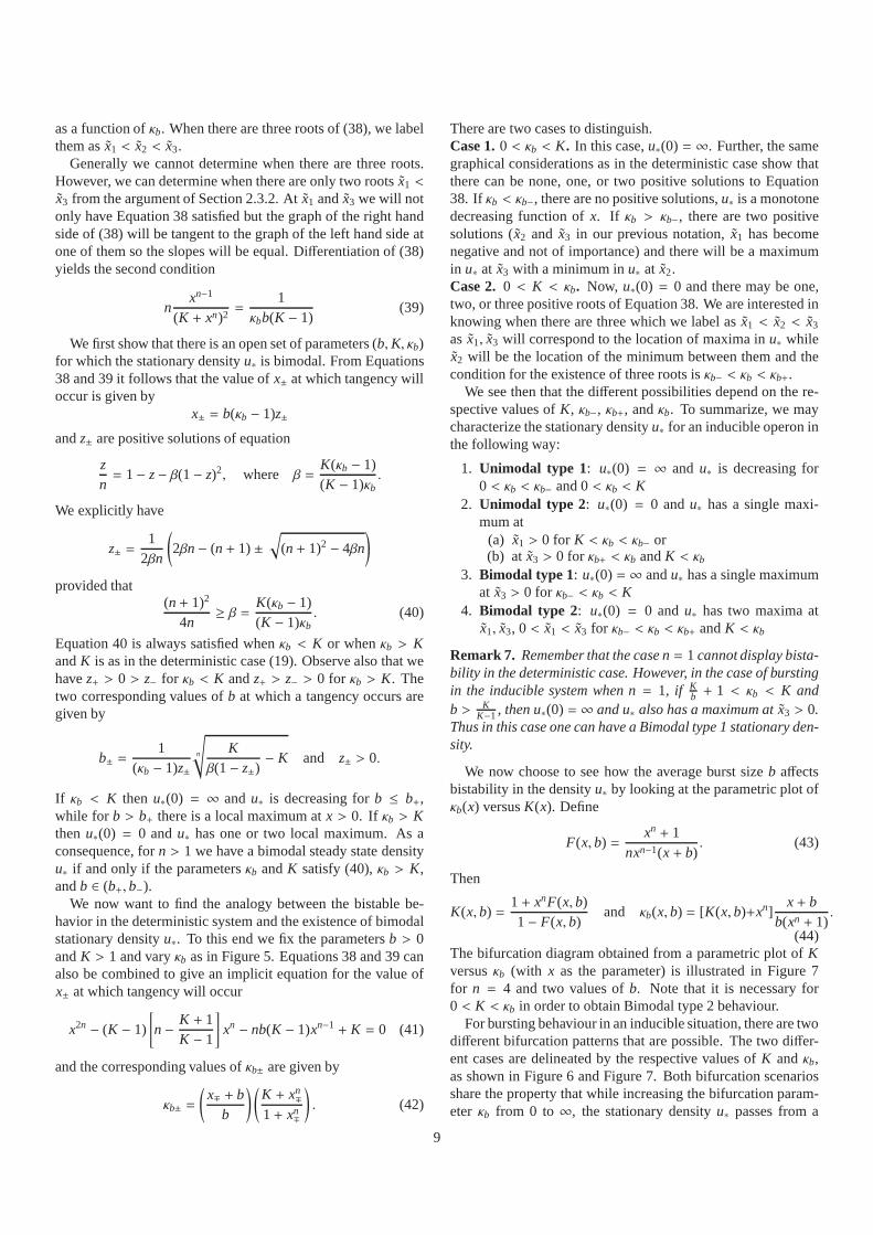
Figure 6: Full logarithmic plot of the values ofx at whichu′∗(x) = 0 versus theparameterκb, obtained from Equation 38, forn = 4, K = 10, and (left to right)b = 5, 1 andb = 1

10. Though somewhat obscured by the logarithmic scale forx,the graphs always intersect theκb axis atκb = K. Additionally, it is importantto note thatu′∗(0) = 0 for K < κb, and that there is always a maximum at 0 for0 < κb < K. See the text for further details.

0 5 10 150

10

20

30

40

50

60

70

K

κb

Figure 7: In this figure we present two bifurcation diagrams (for n = 4) in(K, κb) parameter space delineating unimodal from bimodal stationary densitiesu∗ in an inducible operon with bursting as obtained from Equations 44 with 43.The upper cone-shaped plot is forb = 1

10 while the bottom one is forb = 1. Inboth cone shaped regions, for any situation in which the lower branch is abovethe lineκb = K (lower straight line) then bimodal behaviour in the stationarysolutionu∗(x) will be observed with maxima inu∗ at positive values ofx, x1and x3.

1.5 2 2.5 3 3.5 4

4.44

3.293

2

3.5

5.9

4

K

κb

Figure 8: This figure presents an enlarged portion of Figure 7for b = 1. Thevarious horizontal lines mark specific values ofκb referred to in Figures 9 and10.

unimodal density with a peak at a low value (either 0 or ˜x1) toa bimodal density and then back to a unimodal density with apeak at a high value ( ˜x3).

In what will be referred asBifurcation type 1, the maximumat x = 0 disappears when there is a second peak atx = x3. Thesequence of densities encountered for increasing values ofκb isthen: Unimodal type 1 to a Bimodal type 1 to a Bimodal type 2and finally to a Unimodal type 2 density.

In theBifurcation type 2 situation, the sequence of densitytypes for increasing values ofκb is: Unimodal type 1 to a Uni-modal type 2 and then a Bimodal type 2 ending in a Unimodaltype 2 density.

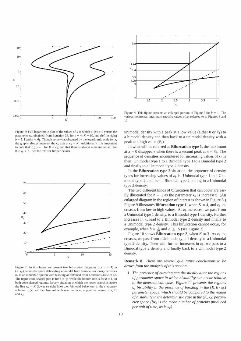
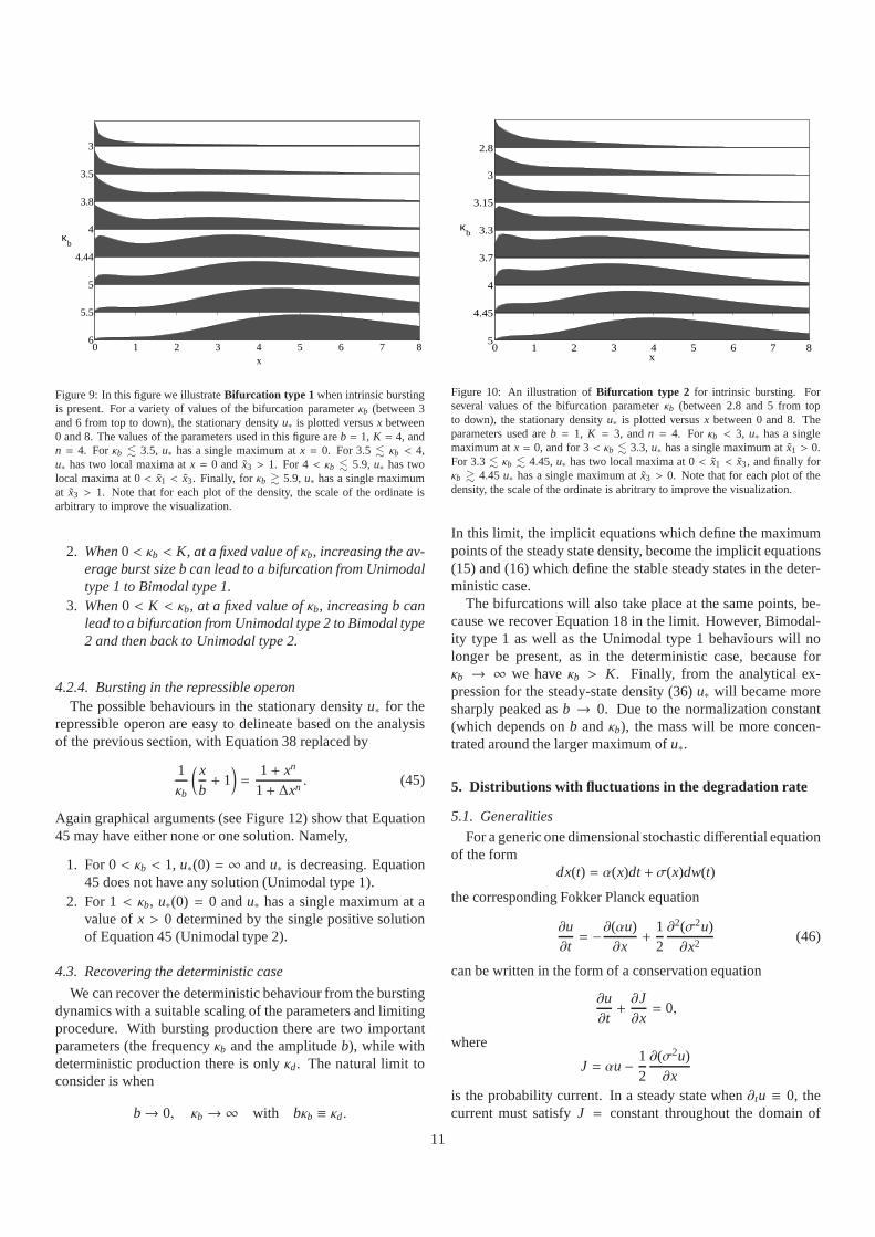
The two different kinds of bifurcation that can occur are eas-ily illustrated forb = 1 as the parameterκb is increased. (Anenlarged diagram in the region of interest is shown in Figure8.)Figure 9 illustratesBifurcation type 1, whenK = 4, andκb in-creases from low to high values. Asκb increases, we pass froma Unimodal type 1 density, to a Bimodal type 1 density. Furtherincreases inκb lead to a Bimodal type 2 density and finally toa Unimodal type 2 density. This bifurcation cannot occur, forexample, whenb = 1

10 andK ≤ 15 (see Figure 7).Figure 10 showsBifurcation type 2, whenK = 3. Asκb in-

creases, we pass from a Unimodal type 1 density, to a Unimodaltype 2 density. Then with further increases inκb, we pass to aBimodal type 2 density and finally back to a Unimodal type 2density.

Remark 8. There are several qualitative conclusions to bedrawn from the analysis of this section.

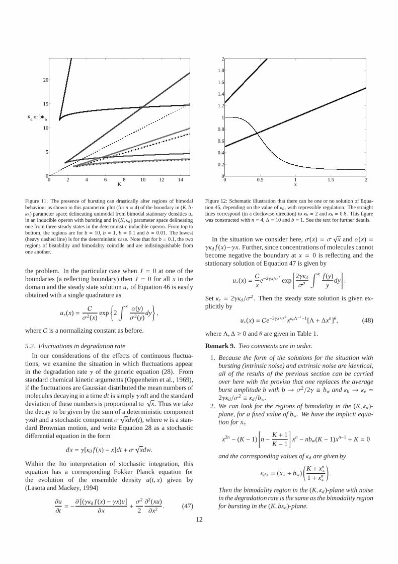
1. The presence of bursting can drastically alter the regionsof parameter space in which bistability can occur relativeto the deterministic case. Figure 11 presents the regionsof bistability in the presence of bursting in the(K, b · κb)parameter space, which should be compared to the regionof bistability in the deterministic case in the(K, κd) param-eter space (bκb is the mean number of proteins producedper unit of time, as isκd)

10

3

3.5

3.8

4

4.44

5

5.5

0 1 2 3 4 5 6 7 86

x

κb

Figure 9: In this figure we illustrateBifurcation type 1 when intrinsic burstingis present. For a variety of values of the bifurcation parameter κb (between 3and 6 from top to down), the stationary densityu∗ is plotted versusx between0 and 8. The values of the parameters used in this figure areb = 1, K = 4, andn = 4. Forκb . 3.5, u∗ has a single maximum atx = 0. For 3.5 . κb < 4,u∗ has two local maxima atx = 0 and x3 > 1. For 4< κb . 5.9, u∗ has twolocal maxima at 0< x1 < x3. Finally, for κb & 5.9, u∗ has a single maximumat x3 > 1. Note that for each plot of the density, the scale of the ordinate isarbitrary to improve the visualization.

2. When0 < κb < K, at a fixed value ofκb, increasing the av-erage burst size b can lead to a bifurcation from Unimodaltype 1 to Bimodal type 1.

3. When0 < K < κb, at a fixed value ofκb, increasing b canlead to a bifurcation from Unimodal type 2 to Bimodal type2 and then back to Unimodal type 2.

4.2.4. Bursting in the repressible operonThe possible behaviours in the stationary densityu∗ for the

repressible operon are easy to delineate based on the analysisof the previous section, with Equation 38 replaced by

1κb

( xb+ 1

)

=1+ xn

1+ ∆xn. (45)

Again graphical arguments (see Figure 12) show that Equation45 may have either none or one solution. Namely,

1. For 0< κb < 1, u∗(0) = ∞ andu∗ is decreasing. Equation45 does not have any solution (Unimodal type 1).

2. For 1< κb, u∗(0) = 0 andu∗ has a single maximum at avalue ofx > 0 determined by the single positive solutionof Equation 45 (Unimodal type 2).

4.3. Recovering the deterministic case

We can recover the deterministic behaviour from the burstingdynamics with a suitable scaling of the parameters and limitingprocedure. With bursting production there are two importantparameters (the frequencyκb and the amplitudeb), while withdeterministic production there is onlyκd. The natural limit toconsider is when

b→ 0, κb → ∞ with bκb ≡ κd.

2.8

3

3.15

3.3

3.7

4

4.45

0 1 2 3 4 5 6 7 85

x

κb

Figure 10: An illustration ofBifurcation type 2 for intrinsic bursting. Forseveral values of the bifurcation parameterκb (between 2.8 and 5 from topto down), the stationary densityu∗ is plotted versusx between 0 and 8. Theparameters used areb = 1, K = 3, andn = 4. For κb < 3, u∗ has a singlemaximum atx = 0, and for 3< κb . 3.3, u∗ has a single maximum at ˜x1 > 0.For 3.3 . κb . 4.45, u∗ has two local maxima at 0< x1 < x3, and finally forκb & 4.45 u∗ has a single maximum at ˜x3 > 0. Note that for each plot of thedensity, the scale of the ordinate is abritrary to improve the visualization.

In this limit, the implicit equations which define the maximumpoints of the steady state density, become the implicit equations(15) and (16) which define the stable steady states in the deter-ministic case.

The bifurcations will also take place at the same points, be-cause we recover Equation 18 in the limit. However, Bimodal-ity type 1 as well as the Unimodal type 1 behaviours will nolonger be present, as in the deterministic case, because forκb → ∞ we haveκb > K. Finally, from the analytical ex-pression for the steady-state density (36)u∗ will became moresharply peaked asb → 0. Due to the normalization constant(which depends onb andκb), the mass will be more concen-trated around the larger maximum ofu∗.

5. Distributions with fluctuations in the degradation rate

5.1. Generalities

For a generic one dimensional stochastic differential equationof the form

dx(t) = α(x)dt+ σ(x)dw(t)

the corresponding Fokker Planck equation

∂u∂t= −∂(αu)

∂x+

12∂2(σ2u)∂x2

(46)

can be written in the form of a conservation equation

∂u∂t+∂J∂x= 0,

where

J = αu−12∂(σ2u)∂x

is the probability current. In a steady state when∂tu ≡ 0, thecurrent must satisfyJ = constant throughout the domain of

11

0 2 4 6 8 10 12 140

5

10

15

20

K

κd or bκ

b

Figure 11: The presence of bursting can drastically alter regions of bimodalbehaviour as shown in this parametric plot (forn = 4) of the boundary in (K, b ·κb) parameter space delineating unimodal from bimodal stationary densitiesu∗in an inducible operon with bursting and in (K, κd) parameter space delineatingone from three steady states in the deterministic inducibleoperon. From top tobottom, the regions are forb = 10, b = 1, b = 0.1 andb = 0.01. The lowest(heavy dashed line) is for the deterministic case. Note thatfor b = 0.1, the tworegions of bistability and bimodality coincide and are indistinguishable fromone another.

the problem. In the particular case whenJ = 0 at one of theboundaries (a reflecting boundary) thenJ = 0 for all x in thedomain and the steady state solutionu∗ of Equation 46 is easilyobtained with a single quadrature as

u∗(x) =Cσ2(x)

exp

{

2∫ x α(y)σ2(y)

dy

}

,

whereC is a normalizing constant as before.

5.2. Fluctuations in degradation rate

In our considerations of the effects of continuous fluctua-tions, we examine the situation in which fluctuations appearin the degradation rateγ of the generic equation (28). Fromstandard chemical kinetic arguments (Oppenheim et al., 1969),if the fluctuations are Gaussian distributed the mean numbers ofmolecules decaying in a timedt is simplyγxdtand the standarddeviation of these numbers is proportional to

√x. Thus we take

the decay to be given by the sum of a deterministic componentγxdt and a stochastic componentσ

√xdw(t), wherew is a stan-

dard Brownian motion, and write Equation 28 as a stochasticdifferential equation in the form

dx= γ[κd f (x) − x]dt+ σ√

xdw.

Within the Ito interpretation of stochastic integration, thisequation has a corresponding Fokker Planck equation forthe evolution of the ensemble densityu(t, x) given by(Lasota and Mackey, 1994)

∂u∂t= −∂

[

(γκd f (x) − γx)u]

∂x+σ2

2∂2(xu)∂x2

. (47)

0 0.5 1 1.5 20

0.2

0.4

0.6

0.8

1

1.2

1.4

1.6

1.8

2

x

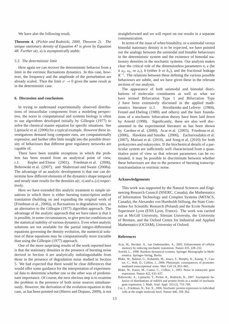
Figure 12: Schematic illustration that there can be one or nosolution of Equa-tion 45, depending on the value ofκb, with repressible regulation. The straightlines correspond (in a clockwise direction) toκb = 2 andκb = 0.8. This figurewas constructed withn = 4,∆ = 10 andb = 1. See the text for further details.

In the situation we consider here,σ(x) = σ√

x andα(x) =γκd f (x)−γx. Further, since concentrations of molecules cannotbecome negative the boundary atx = 0 is reflecting and thestationary solution of Equation 47 is given by

u∗(x) =Cx

e−2γx/σ2exp

[

2γκdσ2

∫ x f (y)y

dy

]

.

Setκe = 2γκd/σ2. Then the steady state solution is given ex-plicitly by

u∗(x) = Ce−2γx/σ2xκeΛ

−1−1[Λ + ∆xn]θ, (48)

whereΛ,∆ ≥ 0 andθ are given in Table 1.

Remark 9. Two comments are in order.

1. Because the form of the solutions for the situation withbursting (intrinsic noise) and extrinsic noise are identical,all of the results of the previous section can be carriedover here with the proviso that one replaces the averageburst amplitude b with b→ σ2/2γ ≡ bw andκb → κe =2γκd/σ2 ≡ κd/bw.

2. We can look for the regions of bimodality in the(K, κd)-plane, for a fixed value of bw. We have the implicit equa-tion for x±

x2n − (K − 1)

[

n− K + 1K − 1

]

xn − nbw(K − 1)xn−1 + K = 0

and the corresponding values ofκd are given by

κd± = (x∓ + bw)

(

K + xn∓

1+ xn∓

)

.

Then the bimodality region in the(K, κd)-plane with noisein the degradation rate is the same as the bimodality regionfor bursting in the(K, bκb)-plane.

12

We have also the following result.

Theorem 4. (Pichor and Rudnicki, 2000, Theorem 2). Theunique stationary density of Equation 47 is given by Equation48. Further u(t, x) is asymptotically stable.

5.3. The deterministic limit

Here again we can recover the deterministic behavior from alimit in the extrinsic fluctuations dynamics. In this case, how-ever, the frequency and the amplitude of the perturbation arealready scaled. Then the limitσ → 0 gives the same result asin the deterministic case.

6. Discussion and conclusions

In trying to understand experimentally observed distribu-tions of intracellular components from a modeling perspec-tive, the norm in computational and systems biology is oftento use algorithms developed initially by Gillespie (1977) tosolve the chemical master equation for specific situations.SeeLipniacki et al. (2006) for a typical example. However thesein-vestigations demand long computer runs, are computationallyexpensive, and further offer little insight into the possible diver-sity of behaviours that different gene regulatory networks arecapable of.

There have been notable exceptions in which the prob-lem has been treated from an analytical point of view,c.f. Kepler and Elston (2001), Friedman et al. (2006),Bobrowski et al. (2007), and Shahrezaei and Swain (2008a).The advantage of an analytic development is that one can de-termine how different elements of the dynamics shape temporaland steady state results for the densitiesu(t, x) andu∗(x) respec-tively.

Here we have extended this analytic treatment to simple sit-uations in which there is either bursting transcription and/ortranslation (building on and expanding the original work of(Friedman et al., 2006)), or fluctuations in degradation rates, asan alternative to the Gillespie (1977) algorithm approach.Theadvantage of the analytic approach that we have taken is thatitis possible, in some circumstances, to give precise conditions onthe statistical stability of various dynamics. Even when analyticsolutions are not available for the partial integro-differentialequations governing the density evolution, the numerical solu-tion of these equations may be computationally more tractablethan using the Gillespie (1977) approach.

One of the more surprising results of the work reported hereis that the stationary densities in the presence of burstingnoisederived in Section 4 are analytically indistinguishable fromthose in the presence of degradation noise studied in Section5. We had expected that there would be clear differences thatwould offer some guidance for the interpretation of experimen-tal data to determine whether one or the other was of predomi-nant importance. Of course, the next obvious step is to examinethe problem in the presence of both noise sources simultane-ously. However, the derivation of the evolution equation inthiscase, as has been pointed out (Hierro and Dopazo, 2009), is not

straightforward and we will report on our results in a separatecommunication.

In terms of the issue of when bistability, or a unimodal versusbimodal stationary density is to be expected, we have pointedout the analogy between the unimodal and bistable behavioursin the deterministic system and the existence of bimodal sta-tionary densities in the stochastic systems. Our analysis makesclear the critical role of the dimensionless parametersn, κ (beit κd, κb, or κe), b (eitherb or bw), and the fractional leakageK−1. The relations between these defining the various possiblebehaviours are subtle, and we have given these in the relevantsections of our analysis.

The appearance of both unimodal and bimodal distri-butions of molecular constituents as well as what wehave termed Bifurcation Type 1 and Bifurcation Type2 have been extensively discussed in the applied math-ematics literature (c.f. Horsthemke and Lefever (1984),Feistel and Ebeling (1989) and others) and the bare founda-tions of a stochastic bifurcation theory have been laid downby Arnold (1998). Significantly, these are also well doc-umented in the experimental literature as has been shownby Gardner et al. (2000), Acar et al. (2005), Friedman et al.(2006), Hawkins and Smolke (2006), Zacharioudakis et al.(2007), Mariani et al. (2010), and Song et al. (2010) for bothprokaryotes and eukaryotes. If the biochemical details of apar-ticular system are sufficiently well characterized from a quan-titative point of view so that relevant parameters can be es-timated, it may be possible to discriminate between whetherthese behaviours are due to the presence of bursting transcrip-tion/translation or extrinsic noise.

Acknowledgements

This work was supported by the Natural Sciences and Engi-neering Research Council (NSERC, Canada), the Mathematicsof Information Technology and Complex Systems (MITACS,Canada), the Alexander von Humboldt Stiftung, the State Com-mittee for Scientific Research (Poland) and the Ecole NormaleSuperieure Lyon (ENS Lyon, France). The work was carriedout at McGill University, Silesian University, the Universityof Bremen, and the Oxford Centre for Industrial and AppliedMathematics (OCIAM), University of Oxford.

References

Acar, M., Becskei, A., van Oudenaarden, A., 2005. Enhancement of cellularmemory by reducing stochastic transitions. Nature 435, 228–232.

Arnold, L., 1998. Random dynamical systems. Springer Monographs in Math-ematics. Springer-Verlag, Berlin.

Blake, W., Balazsi, G., Kohanski, M., Issacs, F., Murphy, K., Kuang, Y., Can-tor, C., Walt, D., Collins, J., 2006. Phenotypic consequences of promoter-mediated transcriptional noise. Mol. Cell 24, 853–865.

Blake, W., Kaern, M., Cantor, C., Collins, J., 2003. Noise ineukaryotic geneexpression. Nature 422, 633–637.

Bobrowski, A., Lipniacki, T., Pichor, K., Rudnicki, R., 2007. Asymptotic be-havior of distributions of mRNA and protein levels in a modelof stochasticgene expression. J. Math. Anal. Appl. 333 (2), 753–769.

Cai, L., Friedman, N., Xie, X., 2006. Stochastic protein expression in individualcells at the single molecule level. Nature 440, 358–362.

13

Chubb, J., Trcek, T., Shenoy, S., Singer, R., 2006. Transcriptional pulsing of adevelopmental gene. Curr. Biol. 16, 1018–1025.

Elowitz, M., Levine, A., Siggia, E., Swain, P., 2002. Stochastic gene expressionin a single cell. Science 297, 1183–1186.

Feistel, R., Ebeling, W., 1989. Evolution of Complex Systems. VEB DeutscherVerlag der Wissenschaften, Berlin.

Fraser, H., Hirsh, A., Glaever, G., J.Kumm, Eisen, M., 2004.Noise minimiza-tion in eukaryotic gene expression. PLoS Biology 2, 8343–838.

Friedman, N., Cai, L., Xie, X. S., 2006. Linking stochastic dynamics to popu-lation distribution: An analytical framework of gene expression. Phys. Rev.Lett. 97, 168302–1–4.

Gardiner, C., 1983. Handbook of Stochastic Methods. Springer Verlag, Berlin,Heidelberg.

Gardner, T., Cantor, C., Collins, J., 2000. Construction ofa genetic toggleswitch in Escherichia coli. Nature 403, 339–342.

Gillespie, D., 1977. Exact stochastic simulation of coupled chemical reactions.J. Phys. Chem. 81, 2340–2361.

Golding, I., Paulsson, J., Zawilski, S., Cox, E., 2005. Real-time kinetics of geneactivity in individual bacteria. Cell 123, 1025–1036.

Griffith, J., 1968a. Mathematics of cellular control processes. I. Negative feed-back to one gene. J. Theor. Biol. 20, 202–208.

Griffith, J., 1968b. Mathematics of cellular control processes. II. Positive feed-back to one gene. J. Theor. Biol. 20, 209–216.

Haken, H., 1983. Synergetics: An introduction, 3rd Edition. Vol. 1 of SpringerSeries in Synergetics. Springer-Verlag, Berlin.

Hawkins, K., Smolke, C., 2006. The regulatory roles of the galactose permeaseand kinase in the induction response of the GAL network in Saccharomycescerevisiae. J. Biol. Chem. 281, 13485–13492.

Hierro, J., Dopazo, C., 2009. Singular boundaries in the forward Chapman-Kolmogorov differential equation. J. Stat. phys. 137, 305–329.

Horsthemke, W., Lefever, R., 1984. Noise Induced Transitions: Theory andApplications in Physics, Chemistry, and Biology. Springer-Verlag, Berlin,New York, Heidelberg.

Kaern, M., Elston, T., Blake, W., Collins, J., 2005. Stochasticity in gene expres-sion: From theories to phenotypes. Nature Reviews Genetics6, 451–464.

Kepler, T., Elston, T., 2001. Stochasticity in transcriptional regulation: Origins,consequences, and mathematical representations. Biophy.J. 81, 3116–3136.

Lasota, A., Mackey, M., 1994. Chaos, fractals, and noise. Vol. 97 of AppliedMathematical Sciences. Springer-Verlag, New York.

Lipniacki, T., Paszek, P., Marciniak-Czochra, A., Brasier, A., Kimmel, M.,2006. Transcriptional stochasticity in gene expression. J. Theoret. Biol.238 (2), 348–367.

Mackey, M. C., Tyran-Kaminska, M., 2008. Dynamics and density evolution inpiecewise deterministic growth processes. Ann. Polon. Math. 94, 111–129.

Mariani, L., Schulz, E., Lexberg, M., Helmstetter, C., Radbruch, A., Lohning,M., Hofer, T., 2010. Short-term memory in gene induction reveals the regu-latory principle behind stochastic IL-4 expression. Mol. Sys. Biol. 6, 359.

Ochab-Marcinek, A., 2008. Predicting the asymmetric response of a geneticswitch to noise. J. Theor. Biol. 254, 37–44.

Ochab-Marcinek, A., 2010. Extrinsic noise passing througha Michaelis-Menten reaction: A universal response of a genetic switch. J. Theor. Biol.263, 510–520.

Oppenheim, I., Schuler, K., Weiss, G., 1969. Stochastic anddeterministic for-mulation of chemical rate equations. J. Chem. Phys. 50, 460–466.

Othmer, H., 1976. The qualitative dynamics of a class of biochemical controlcircuits. J. Math. Biol. 3, 53–78.

Pichor, K., Rudnicki, R., 2000. Continuous Markov semigroups and stability oftransport equations. J. Math. Anal. Appl. 249, 668–685.

Polynikis, A., Hogan, S., di Bernardo, M., 2009. Comparing differeent ODEmodelling approaches for gene regulatory networks. J. Theor. Biol. 261,511–530.

Raj, A., Peskin, C., Tranchina, D., Vargas, D., Tyagi, S., 2006. StochasticmRNA synthesis in mammalian cells. PLoS Biol. 4, 1707–1719.

Raj, A., van Oudenaarden, A., 2008. Nature, nurture, or chance: Stochasticgene expression and its consequences. Cell 135, 216–226.

Raser, J., O’Shea, E., 2004. Control of stochasticity in eukaryotic gene expres-sion. Science 304, 1811–1814.

Scott, M., Ingallls, B., Kærn, M., 2006. Estimations of intrinsic and extrinsicnoise in models of nonlinear genetic networks. Chaos 16, 026107–1–15.

Selgrade, J., 1979. Mathematical analysis of a cellular control process withpositive feedback. SIAM J. Appl. Math. 36, 219–229.

Shahrezaei, V., Ollivier, J., Swain, P., 2008. Colored extrinsic fluctuations andstochastic gene expression. Mol. Syst. Biol. 4, 196–205.

Shahrezaei, V., Swain, P., 2008a. Analytic distributions for stochastic gene ex-pression. Proc. Nat. Acad. Sci 105, 17256–17261.

Shahrezaei, V., Swain, P., 2008b. The stochastic nature of biochemical net-works. Cur Opinion Biotech 19, 369–374.

Sigal, A., Milo, R., Cohen, A., Geva-Zatorsky, N., Klein, Y., Liron, Y., Rosen-feld, N., Danon, T., Perzov, N., Alon, U., 2006. Variabilityand memory ofprotein levels in human cells. Nature 444, 643–646.

Smith, H., 1995. Monotone Dynamical Systems. Vol. 41 of Mathematical Sur-veys and Monographs. American Mathematical Society, Providence, RI.

Song, C., Phenix, H., Abedi, V., Scott, M., Ingalls4, B., Perkins, M. K. T.,2010. Estimating the stochastic bifurcation structure of cellular networks.PLos Comp. Biol. 6, e1000699/1–11.

Stratonovich, R. L., 1963. Topics in the theory of random noise. Vol. I: Gen-eral theory of random processes. Nonlinear transformations of signals andnoise. Revised English edition. Translated from the Russian by Richard A.Silverman. Gordon and Breach Science Publishers, New York.

Swain, P., Elowitz, M., Siggia, E., 2002. Intrinsic and extrinsic contributions tostochasticity in gene expression. Proc Nat Acad Sci 99, 12795–12800.

Titular, U., 1978. A systematic solution procedure for the Fokker-Planck equa-tion of a Brownian particle in the high-friction case. Physica 91A, 321–344.

Wilemski, G., 1976. On the derivation of Smoluchowski equations with correc-tions in the classical theory of Brownian motion. J. Stat. Phys. 14, 153–169.

Yildirim, N., Santillan, M., Horike, D., Mackey, M. C., 2004. Dynamics andbistability in a reduced model of thelac operon. Chaos 14, 279–292.

Yu, J., Xiao, J., Ren, X., Lao, K., Xie, X., 2006. Probing geneexpression inlive cells, one protein molecule at a time. Science 311, 1600–1603.

Zacharioudakis, I., Gligoris, T., Tzamarias, D., 2007. A yeast catabolic enzymecontrols transcriptional memory. Current Biology 17, 2041–2046.

14