Diploma Thesis Structural Mechanics SAMUEL BLUMER MOISTURE INDUCED STRESSES AND DEFORMATIONS IN PARQUET FLOORS - An Experimental and Numerical Study

Welcome message from author
This document is posted to help you gain knowledge. Please leave a comment to let me know what you think about it! Share it to your friends and learn new things together.
Transcript
Diploma ThesisStructural
Mechanics
SAMUEL BLUMER
MOISTURE INDUCED STRESSESAND DEFORMATIONS IN PARQUETFLOORS - An Experimental andNumerical Study

Detta är en tom sida!
Copyright © 2006 by Structural Mechanics, LTH, Sweden.Printed by KFS I Lund AB, Lund, Sweden, March 2006.
For information, address:
Division of Structural Mechanics, LTH, Lund University, Box 118, SE-221 00 Lund, Sweden.Homepage: http://www.byggmek.lth.se
Structural MechanicsDepartment of Construction Sciences
Diploma Thesis by
SAMUEL BLUMER
Supervisors:
Dr. Erik Serrano and Prof. Per Johan Gustafsson,Div. of Structural Mechanics
MOISTURE INDUCED STRESSES AND
DEFORMATIONS IN PARQUET FLOORS
- An Experimental and Numerical Study
ISRN LUTVDG/TVSM--06/5143--SE (1-94)ISSN 0281-6679
Prof. Peter Niemz,Institute for Building Materials, Wood Physics,
ETH-Hönggerberg, Zürich, Switzerland

i
Abstract
The indoor climate conditions in buildings have changed in the last decade due to more efficient climatic systems, floor heating systems and larger open floor areas with more natural light. These factors all give increased annual variations in the humidity and the temperature in parquet floors. Such variations can result in troublesome deformations, glue line delamination and development of cracks in the parquet flooring boards. In this master’s dissertation, the possibility of using the finite element method for deformation and failure prediction of parquet floors under changing climatic conditions was investigated. Several finite element models and also a simple beam model were created and applied. In addition, several experimental tests were made to study the deformation performance of parquet boards and to determine material parameters and to get information for calibration and validation of the theoretical model. After calibration and validation of the calculation method, parameter studies on the influence of material properties, geometry of the parquet floors and the long-term behaviour of the wood and glue line were performed in order to increase the understanding of the behaviour of parquet floors under changing climate. The results showed that the deformations and the stresses are strongly affected by the properties of the materials and by the geometrical design of the parquet boards. The deformations that are strongly affected include the gap opening. The stresses found may result in delamination of the surface layer. A parameter study of the long time behaviour of the parquet planks resulted in better understanding of the influence of creeping on the aforesaid deformations and failure modes. Keywords: parquet floor, finite element method, moisture, temperature, stress distribution,

ii
iii
Acknowledgements
This diploma thesis was carried out during the winter of 2005/2006 at the Division of Structural Mechanics at Lund University in corporation with the Institute of Building Materials at the Swiss Federal Institute of Technology in Zurich and Tarkett AB in Hanaskog. I would especially like to thank my supervisors Prof. Peter Niemz, Prof. Per Johan Gustafsson and Dr. Erik Serrano for their expert guidance and support. I wish to thank Anna-Lena Gull from Tarkett AB for providing the project with test material and technical information. I am also grateful to Thord Lundgren for construction of the testing installation, Eva Frühwald from the Division of Structural Engineering for the use of the climatic chamber, Walter Sonderegger for his guidance and support of the experimental part provided in Zurich and all the staff from the Division of Structural Mechanics in Lund and Building Materials in Zurich who assisted me in many ways during the work. A special thank to my sister Claudia for reviewing the thesis English. Lund, 3 February 2006 Samuel Blumer

iv
v
Zusammenfassung
Seit den siebziger Jahren ist der Anteil an Parkettböden in Wohn- und Industriebauten stetig gestiegen. Klimaanlagen und Bodenheizsysteme aber auch die Zeitströmung zu immer grösseren Räumen haben die Amplitude der saisonal bedingten Schwankungen der Luftfeuchte ansteigen lassen. Vor allem bei trockener Winterluft gekoppelt mit dem Wärmeeintrag einer Bodenheizung sinkt der Feuchtegehalt im Holz auf absolute Tiefwerte. Das führt zu Fugenöffnung, Wölbungen und zum Ablösen der Deckschicht. Die Dimensionierung und konstruktive Ausbildung der Parkettelemente erfolgte bisher über Laborversuche und Freilanderfahrungen. Oft werden auch die Konzepte der Konkurrenzprodukte kopiert und deren Schwächen übernommen. In dieser Diplomarbeit wird mit der Methode der Finiten Elemente ein neues Werkzeug für die Dimensionierung und für die konstruktive Ausformung der Parkette und deren Verbindungen untereinander vorgestellt. Verschiedene Berechnungsverfahren mit Variation der Annahmen wurden untersucht um das Wölben der Elemente, das Öffnen und Schliessen der Fugen sowie den Spannungsaufbau in den Leimfugen modellieren zu können. Begonnen wurde mit einem Modell, das auf Messungen aufgebaut wurde. Dieses diente der eigentlichen Kalibrierung über das Anpassen von Annahmen und Berechnungsmethoden. Für die Versuche wurden Produkte der Firma Tarkett AB eingesetzt. Die geprüften Probekörper hatten einen Aufbau von unten nach oben beginnend mit einem 2 mm starken Furnierschichtholz (Pinus sylvestris L.), danach mit der Mittellage âus 8.6 mm Föhreleisten (Pinus sylvestris L.) und mit einer 3.6 mm dicken Deckschicht aus Eichenbrettchen (Quercus robur L.). Die einzelnen Schichten werden mit Harnstoffharz in einer Hochfrequenzpresse bei einer Temperatur bis zu 90° rechtwinklig zu einander verleimt. Aus den Versuchen mit dem Grundmaterial konnten die wichtigsten Materialparameter wie der E-Modul in Längsrichtung und die Schwind- und Quellfaktoren ermittelt werden. Die Resultate aus den Berechnungen über Finite Elemente wurden mit den Verformungsmessungen an 15x15 cm grossen Platten verglichen und kalibriert. Der Einfluss der Jahringstellung auf das Verformungsverhalten war beträchtlich. Anders formuliert war es dieser Parameter, welcher bei Kurzzeitbelastung die grösste Auswirkung auf das Verformungsverhalten hatte. Da Schäden in Parkettböden vor allem in trockenen Wintern auftraten, wurde bei den Annahmen von einem eigenspannungsfreien Parket von 7.5% Feuchtegehalt ausgegangen, das ist die Feuchte welche die Parkette am Ende der Produktion aufweisen. Die Modelle wurden anschliessend auf ein Niveau von 5% Feuchtegehalt heruntergerechnet und die Verformungen und Spannungen ermittelt. Für das Abschätzen des Ausmasses des Feuchtigkeitstransportes wurde ein Diffusionskoeffizient mit zu Hilfenahme der Versuchsresulate bestimmt. Der Einfluss der Leimfugen auf den Feuchtetransport konnte nicht ermittelt werden. Die Leimfugen sind für das Verformungsverhalten aber von grosser Bedeutung. Wirkt die Leimschicht als Feuchtigkeitsbremse, dann nehmen die Wölbverformungen um 25% zu. Das heisst das
vi ein grosser Teil der Feuchte in der Decklage durch die darunter liegende Leimschicht blockiert ist. Um Verformungen schnell berechnen zu können, wurde ein Balkenmodell zu Hilfe genommen, welches erlaubte, die Berechnungen mit Finiten Elementen und den Versuchsresultaten zu vergleichen und realitätsbezogene Verformungsabschätzungen zu bekommen. Um das Verhalten der Parkettböden besser verstehen zu können und die Spannungszustände zu erfassen, wurden die Eingabedaten wie die Materialkonstanten, die Geometrie, die Winkel der Jahrringe und die Kriechfaktoren variiert. Bei der Spannungsanalyse konnten die Steigungen der Kurven verglichen werden. Eine Bruchanalyse habe ich im Rahmen der Diplomarbeit nicht durchgeführt, sie wäre aber sehr hilfreich um die Ablösung der Deckschicht besser erklären zu können. Ein Versuch mit dem Modellieren eines plastischen Verhaltens der Leimfuge brachte keinen großen Einfluss auf die Spannungsverteilungen. Das Harnstoffharz ist wahrscheinlich weniger hygroskopisch als das angrenzende Holz.
vii
Sammanfattning
Andelen trägolv i nybyggnation har under det senaste decenniet ökat kraftigt. Samtidigt som andelen trägolv i våra bostäder och industribyggnader ökat, har en ökad användning av golvvärmesystem och tendensen till större och ljusare rum medfört ökade fuktamplituder i inomhusluften under året. Detta tillsammans med väl isolerade hus har medfört ett gradvis torrare inomhusklimat. Fuktighet i de olika träskikten i trägolv minskar vilket påverkar risken för skador som öppning av fogar, kupning av golvplank och delaminering av täckskiktet. Dimensionering av golvvärmesystem i kombination med parkettgolv och lösandet av konstruktiva detaljer har i huvudsak gjorts med hjälp av laboratorieförsök och baserat på erfarenhet. I föreliggande examensarbete används finita elementmetoden (FEM) som ett nytt verktyg för att genomföra dimensionering och konstruktiv utforming av parkettgolv och fogen mellan parkettgolvets olika skikt. Numerisk modellering av olika material, variabel geometri och träets egenskaper under långtidsbelastning har genomförts i 2 och 3 dimensioner. De olika parametrarna inverkar på fogöppning, kupning och delaminering av täckskiktet. Inledningsvis användes en FE-modell med samma geometri som de provkroppar som använts vid laboratorieförsök. Deformations- och fuktkvotsmätningar på provbitarna användes för kalibrering av FE-modellen och beräkningsmetoden. Provbitarna var tagna ur en treskikts parkettbräda tillverkad av Tarkett AB, Hansakog. Parketprädorna består underifrån av ett 2mm tjockt furuskikt (Pinus sylvestris L.), ett 8.6mm tjockt furumellanskikt (Pinus sylvestris L.) och ett 3.6mm tjock ektäckskikt (Quercus robur L). De olika skikten är rätvinkligt sammanlimmade med ett urea formaldehyd lim (UF). Materialparametrarna för de olika skiktens grundmaterial, furu och ek, bestämdes. Elasticitetsmodulen, hygroexpansionskoefficienten och materialets vikt vid olika fuktinnehåll mättes. FE-beräkningar jämfördes med och kalibrerats mot de 15x15cm stora parkettplattor som användes vid provningarna. Inverkan av täckskiktets årsringsorientering på nedböjning och horisontell deformation var mycket stor. Denna parameter var den enskilt viktigaste för korttidsdeformationen. Flest skador uppkommer i parkettgolv i det torrare vinterklimatet. Därför har beräkningar på parkettplank inklusive klickfog genomförts på sänkning av träets fuktinnehåll från 7.5% ner till 5%. Förskjutningar och spänningar har därför beräknats efter en teoretisk sänkning av fuktkvoten på 2.5%. En effektiv fukttransportkoefficient har beräknats och jämförts med mätningarna av träets fuktinnehåll. Inverkan av limfogen på fukttransporten har inte bestämts separat. Limfogen har stor betydelse för förskjutnings- och nedböjningsbeteendet. Limfogen, vilken verkar som en barriär för fukttransport, ökar böjdeformationerna hos plattorna med ungefär 25%. Detta eftersom uttorkningen påverkar i första hand täckskiktet och fukttransporten endast sker fram till första limfogen.
viii En beräkningsmodell baserad på balkteori har utvecklas för att uppskatta deformationer och jämföra med FE-beräkningar. Spänningar i limfogen och i parkettbrädan har beräknats med olika material- geometri- och krypningsparametrar för att få en ökad förståelse av parkettens beteende. Resultatkurvorna från beräkningar med olika indata har jämförts med varandra för att se inverkan på spänningsfördelningar och deformationer. En optimering av parameterar kan därmed göras med målet att få bättre beständighet hos produkterna. En försök att införa krypning i limfogen har inte påverkat spänningsfördelningen på ett avgörande sätt. Formaldehydlim har kanske ett mindre hygroskopisk beteende än det intilliggande träet.
ix
Contents
1. Introduction ...................................................................................................... 1
1.1 Background ..................................................................................................... 1 1.2 Objective ......................................................................................................... 2 1.3 Limitations ...................................................................................................... 2 1.4 Outline of the thesis......................................................................................... 3
2. Theoretical background ...................................................................................... 5
2.1 Introduction .................................................................................................... 5 2.2 Wood and its properties................................................................................... 5 2.2.1 Structure of wood ...................................................................................... 5 2.2.2 The orthotropic nature of wood................................................................. 6 2.2.3 Mass density and moisture content ............................................................ 6 2.2.4 Mechanical properties of wood ................................................................ 10 2.2.5 The formation of the total strain.............................................................. 11
2.3 Parquet floors ................................................................................................ 13 2.3 Beam theory .................................................................................................. 14 2.4 Modelling of moisture movement in wood .................................................... 16 2.5.1 Formulation............................................................................................. 16 2.5.2 Similarity of the moisture transport to a temperature field ....................... 18
3. Experimental tests ............................................................................................ 19
3.1 Introduction .................................................................................................. 19 3.2 Tests on basic material ................................................................................... 19 3.2.1 Sorptional behaviour and density ............................................................. 19 3.2.2 E-Modulus............................................................................................... 22 3.2.3 Hygroexpansion....................................................................................... 23
3.3 Tests on 150x150mm parquet squares ........................................................... 26 3.3.1 Matherial and methods ............................................................................ 26 3.3.2 Results and discussion.............................................................................. 29 3.3.3 Failures modes after oven drying.............................................................. 30
4. Calibration and validation ................................................................................ 33
4.1 Introduction .................................................................................................. 33 4.2 Calibration of the moisture transport............................................................. 33 4.2.1 Methods and material .............................................................................. 34 4.2.2 Results and discussion.............................................................................. 37
4.3 Modelling of the test square samples .............................................................. 38 4.3.1 Methods and material .............................................................................. 38 4.3.2 Results and discussion.............................................................................. 41
4.4 Conclusion .................................................................................................... 45
x 5. Modelling of a single parquet plank .................................................................. 47
5.1 Introduction .................................................................................................. 47 5.2 Methods and material .................................................................................... 47 5.2.1 Numerical model in ABAQUS ................................................................ 47 5.2.2 Parameter study ....................................................................................... 48
5.3 Results and discussion.................................................................................... 51 5.3.1 Influence of the coefficients of diffusion .................................................. 51 5.3.2 Creeping in the layers and the glue line.................................................... 52 5.3.3 Design criterion: cupping of the planks.................................................... 53
5.4 Conclusions ................................................................................................... 54 6. Modelling of a parquet floor system .................................................................. 55
6.1 Introduction .................................................................................................. 55 6.2 Methods and material .................................................................................... 55 6.2.1 Numerical model in ABAQUS ................................................................ 55 6.2.2 Parameter study ....................................................................................... 56
6.3 Results and discussion.................................................................................... 58 6.3.3 Design criterion: Middle gap opening...................................................... 58 6.3.4 Stress analysis........................................................................................... 61
6.4 Conclusions ................................................................................................... 66 7. Concluding remarks ......................................................................................... 67
7.1 Conclusions ................................................................................................... 67 7.2 Proposal for future work ................................................................................ 68
Bibliography ........................................................................................................ 69 Appendix A: Beam Theory.................................................................................... 71 Appendix B: Experimental results ......................................................................... 77
B.1 Tests on basic material: Sorption behaviour ................................................... 77 B.2 Tests on basic material: Hygroexpansion........................................................ 79 B.3 Tests on basic material: 3 point bending ........................................................ 81 B.4 Tests on 150x150 parquet squares: Failures ................................................... 82 B.5 Tests on 150x150 parquet squares: Bending .................................................. 83
1
Chapter 1
Introduction
1.1 Background During the last decade the use of wood flooring systems in Sweden and Europe has increased dramatically. In Sweden the proportion of wood flooring rose steadily from 30 % in the seventies its current 80 %. This rapid growth has resulted in development of new products, enabling the industry to maintain and increase its market share. Due to the high capital costs, the development of wood flooring systems is generally dependant on in-house equipment. Sometimes, design is also inspired by other products on the market. In this case unfortunately, design errors can be transmitted and reproduced. More efficient heating and climate control systems are now available on the market. More efficient ventilation systems and endeavouring to reach a more pleasant indoor climate has resulted in a higher indoor relative humidity (RH) range at the service limit state. The Swedish dry winter climate and higher relative humidity leads to an indoor relative humidity range between 20 and 80%, e.g. Kjellberg [10]. The higher relative humidity range, more efficient heating systems and the harsher climate, causes deformations and stresses to occur in the planks. Also the planning of residential areas has changed from smaller rooms and closed spaces to large open living areas with large windows to improve lighting. All this has resulted in the prerequisite for wooden flooring being changed. Warmer floors, drier indoor climate and larger open floor areas have lead to an increased number of problems related to deformations, cracking and delaminating. The introduction of click joints in recent years has been important. This has led to simpler installation of parquet planks; however the click joints have lower strength and stiffness, which means that deformation is higher compared to glued joints, e.g. Tüfekcioglu [21]. Gaps can occur on the surface after long drying periods. Sometimes there is only deterioration of the appearance but the durability of the parquet and the flooring system can also be reduced. Many laboratory tests have to be done before reaching an optimal design of the parquet elements. Due to the high costs, other supplementary research methods should be tested and evaluated. The finite element method (FEM), an approximate method for solving systems of differential equations, has been adopted in the context of this diploma thesis. It should enable a clearer understanding of the behaviour of wood flooring systems under changing climates and the resulting damages. Each situation desired, considerable exaggerated material properties for example, and its influences on parquet products can be simulated. However, the use of finite element models provides options for design purposes of wood flooring systems.
2 CHAPTER 1. INTRODUCTION
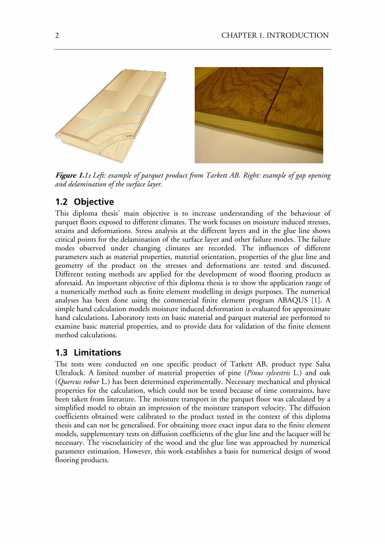
Figure 1.1: Left: example of parquet product from Tarkett AB. Right: example of gap opening and delamination of the surface layer.
1.2 Objective This diploma thesis’ main objective is to increase understanding of the behaviour of parquet floors exposed to different climates. The work focuses on moisture induced stresses, strains and deformations. Stress analysis at the different layers and in the glue line shows critical points for the delamination of the surface layer and other failure modes. The failure modes observed under changing climates are recorded. The influences of different parameters such as material properties, material orientation, properties of the glue line and geometry of the product on the stresses and deformations are tested and discussed. Different testing methods are applied for the development of wood flooring products as aforesaid. An important objective of this diploma thesis is to show the application range of a numerically method such as finite element modelling in design purposes. The numerical analyses has been done using the commercial finite element program ABAQUS [1]. A simple hand calculation models moisture induced deformation is evaluated for approximate hand calculations. Laboratory tests on basic material and parquet material are performed to examine basic material properties, and to provide data for validation of the finite element method calculations.
1.3 Limitations The tests were conducted on one specific product of Tarkett AB, product type Salsa Ultralock. A limited number of material properties of pine (Pinus sylvestris L.) and oak (Quercus robur L.) has been determined experimentally. Necessary mechanical and physical properties for the calculation, which could not be tested because of time constraints, have been taken from literature. The moisture transport in the parquet floor was calculated by a simplified model to obtain an impression of the moisture transport velocity. The diffusion coefficients obtained were calibrated to the product tested in the context of this diploma thesis and can not be generalised. For obtaining more exact input data to the finite element models, supplementary tests on diffusion coefficients of the glue line and the lacquer will be necessary. The viscoelasticity of the wood and the glue line was approached by numerical parameter estimation. However, this work establishes a basis for numerical design of wood flooring products.
CHAPTER 1. INTRODUCTION 3 1.4 Outline of the thesis In the present work, finite element simulations of the deformation and stress in layered parquet planks during moisture variation were performed. The diploma thesis consists of the following chapters: In chapter 2, an introduction to the material properties of wood and composite products like wooden parquet flooring is provided. Chapter 3 consists of experimental tests performed at the Swiss Federal Institute of Technology in Zurich and at Lund University. The material, methods and results are presented and discussed in this chapter. Detailed experimental results are reported in appendix B. Validation of the finite element model is of considerable importance and discussed in chapter 4. Parameter estimation concerning material properties and moisture transport is also considered. A design example of a tested product is checked in terms of distortional effects in chapter 5. In chapter 6, the use of finite elements for specific design purposes of wood flooring systems including click joint is demonstrated. Parameter study of geometry material and glue line completes the chapter. In chapter 7, some concluding remarks are made and various ideas on future research are outlined.

4 CHAPTER 1. INTRODUCTION
5
Chapter 2
Theoretical background
2.1 Introduction The aim of this chapter is to give a brief overview of wood and composite wood products. The main subject of this thesis concerns with wood flooring products such as parquet elements based on solid and veneer timber. Dimensional stability is of high importance in its use and a thorough knowledge of material properties is required. Parquet is comprised of different layers: backing layer, core layer and surface layer. Each layer has its own specific mechanical and physical properties which will be looked at later in this chapter. The layers are glued together with urea formaldehyde resin (UF resin). Under the hardening of the glue in the gluing processes, a composite wood-resin product is built. The properties of these new layers are difficult to determine and have to be estimated. A discussion about the UF resin and its composites is essential. Different calculation methods have been used in the scope of this diploma thesis. An evaluation of a hand calculation model and the comparison to finite element method is given in the second part of the chapter.
2.2 Wood and its properties Wood is one of the oldest structural materials and has been used in many construction fields. It is a renewable resource that requires a small amount of energy to produce; it is available in nearly every part of the world and saves transport energy. Information on the structure of wood is mainly based on the wood handbook [22] and Bodig and Jayne [5]. More detailed information can be found in these textbooks.
2.2.1 Structure of wood Timber is classified into two main groups: conifers also called softwoods and deciduous also called hardwoods. Hardwoods differ between the arrangements of the pores in the cross section: diffuse porous, semi-ring and ring porous. In the context of this thesis the most commonly used terminology of softwoods and hardwoods is used. The most accurate distinction between them is based on anatomical characteristics, e.g. Bodig and Jayne [5]. Factors like the climatic conditions, exposition of the tree, soil composition and climatic conditions have a considerable influence on the material properties of wood and its behaviour. Thus, hard- and softwood differs from one tree to another even within the same species. The variability was also observed in the experimental section of this diploma thesis, c.f. chapter 3. Each species includes a number of functional structures which are different between hard- and softwood. Softwoods are composed of tracheids and parenchyma cells. In
6 CHAPTER 2. THEORETICAL BACKGROUND
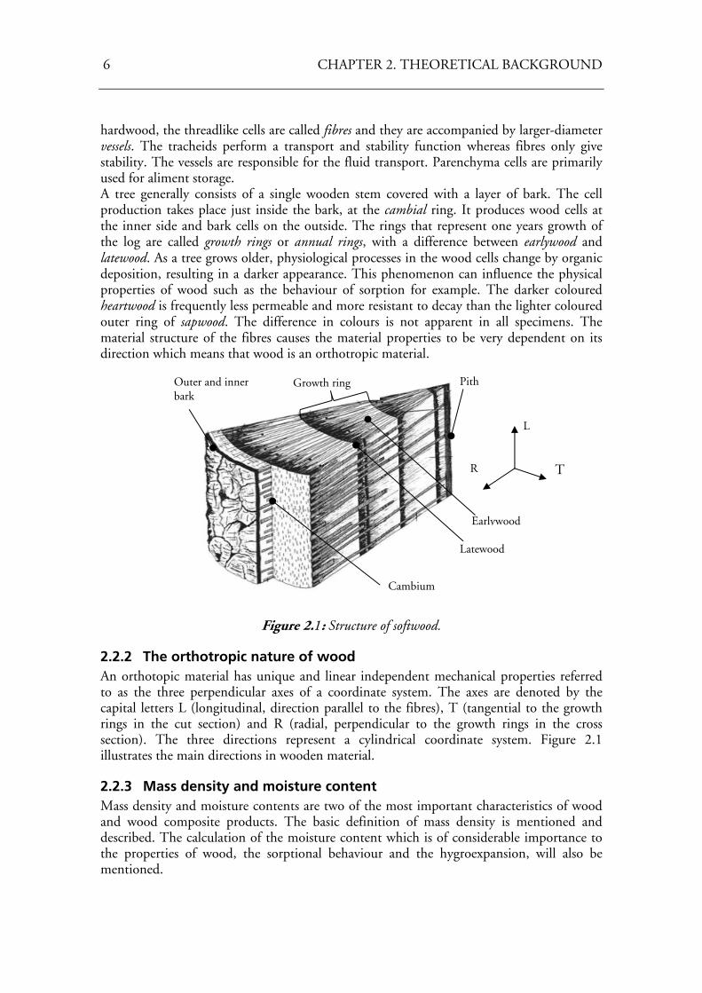
hardwood, the threadlike cells are called fibres and they are accompanied by larger-diameter vessels. The tracheids perform a transport and stability function whereas fibres only give stability. The vessels are responsible for the fluid transport. Parenchyma cells are primarily used for aliment storage. A tree generally consists of a single wooden stem covered with a layer of bark. The cell production takes place just inside the bark, at the cambial ring. It produces wood cells at the inner side and bark cells on the outside. The rings that represent one years growth of the log are called growth rings or annual rings, with a difference between earlywood and latewood. As a tree grows older, physiological processes in the wood cells change by organic deposition, resulting in a darker appearance. This phenomenon can influence the physical properties of wood such as the behaviour of sorption for example. The darker coloured heartwood is frequently less permeable and more resistant to decay than the lighter coloured outer ring of sapwood. The difference in colours is not apparent in all specimens. The material structure of the fibres causes the material properties to be very dependent on its direction which means that wood is an orthotropic material.
Figure 2.1: Structure of softwood.
2.2.2 The orthotropic nature of wood An orthotopic material has unique and linear independent mechanical properties referred to as the three perpendicular axes of a coordinate system. The axes are denoted by the capital letters L (longitudinal, direction parallel to the fibres), T (tangential to the growth rings in the cut section) and R (radial, perpendicular to the growth rings in the cross section). The three directions represent a cylindrical coordinate system. Figure 2.1 illustrates the main directions in wooden material.
2.2.3 Mass density and moisture content Mass density and moisture contents are two of the most important characteristics of wood and wood composite products. The basic definition of mass density is mentioned and described. The calculation of the moisture content which is of considerable importance to the properties of wood, the sorptional behaviour and the hygroexpansion, will also be mentioned.
Outer and inner bark
Cambium
PithGrowth ring
Latewood
Earlywood
R
L
T
CHAPTER 2. THEORETICAL BACKGROUND 7
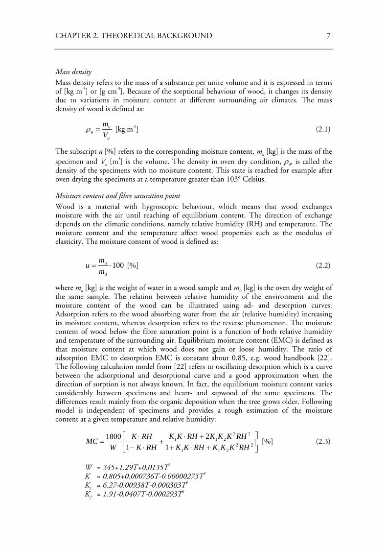
Mass density Mass density refers to the mass of a substance per unite volume and it is expressed in terms of [kg m-3] or [g cm-3]. Because of the sorptional behaviour of wood, it changes its density due to variations in moisture content at different surrounding air climates. The mass density of wood is defined as:
u
uu V
m=ρ [kg m-3] (2.1)
The subscript u [%] refers to the corresponding moisture content, mu [kg] is the mass of the specimen and Vu [m
3] is the volume. The density in oven dry condition, ρ0, is called the density of the specimens with no moisture content. This state is reached for example after oven drying the specimens at a temperature greater than 103° Celsius.
Moisture content and fibre saturation point Wood is a material with hygroscopic behaviour, which means that wood exchanges moisture with the air until reaching of equilibrium content. The direction of exchange depends on the climatic conditions, namely relative humidity (RH) and temperature. The moisture content and the temperature affect wood properties such as the modulus of elasticity. The moisture content of wood is defined as:
1000
⋅=mm
u u [%] (2.2)
where mu [kg] is the weight of water in a wood sample and m0 [kg] is the oven dry weight of the same sample. The relation between relative humidity of the environment and the moisture content of the wood can be illustrated using ad- and desorption curves. Adsorption refers to the wood absorbing water from the air (relative humidity) increasing its moisture content, whereas desorption refers to the reverse phenomenon. The moisture content of wood below the fibre saturation point is a function of both relative humidity and temperature of the surrounding air. Equilibrium moisture content (EMC) is defined as that moisture content at which wood does not gain or loose humidity. The ratio of adsorption EMC to desorption EMC is constant about 0.85, e.g. wood handbook [22]. The following calculation model from [22] refers to oscillating desorption which is a curve between the adsorptional and desorptional curve and a good approximation when the direction of sorption is not always known. In fact, the equilibrium moisture content varies considerably between specimens and heart- and sapwood of the same specimens. The differences result mainly from the organic deposition when the tree grows older. Following model is independent of specimens and provides a rough estimation of the moisture content at a given temperature and relative humidity:
⎥⎦
⎤⎢⎣
⎡+⋅+
+⋅+
⋅−⋅
= 22211
22211
12
11800
RHKKKRHKKRHKKKRHKK
RHKRHK
WMC [%] (2.3)
W = 345+1.29T+0.0135T2
K = 0.805+0.000736T-0.00000273T2
K1 = 6.27-0.00938T-0.000303T2 K2 = 1.91-0.0407T-0.000293T2
8 CHAPTER 2. THEORETICAL BACKGROUND
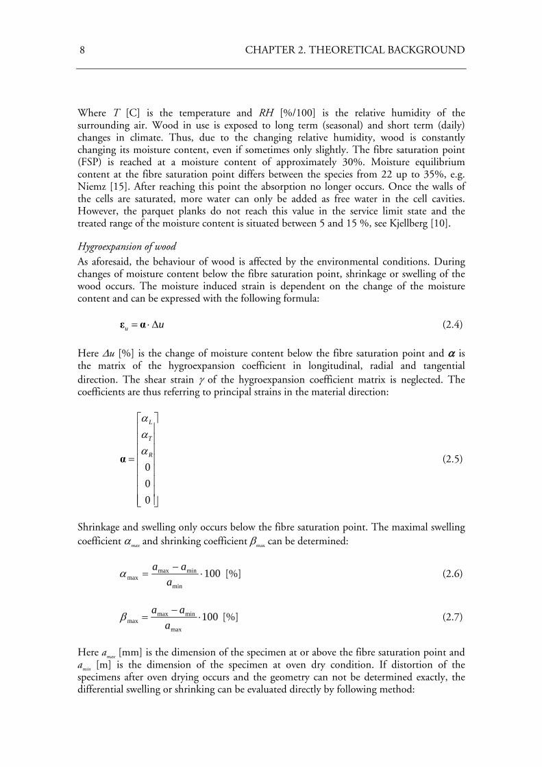
Where T [C] is the temperature and RH [%/100] is the relative humidity of the surrounding air. Wood in use is exposed to long term (seasonal) and short term (daily) changes in climate. Thus, due to the changing relative humidity, wood is constantly changing its moisture content, even if sometimes only slightly. The fibre saturation point (FSP) is reached at a moisture content of approximately 30%. Moisture equilibrium content at the fibre saturation point differs between the species from 22 up to 35%, e.g. Niemz [15]. After reaching this point the absorption no longer occurs. Once the walls of the cells are saturated, more water can only be added as free water in the cell cavities. However, the parquet planks do not reach this value in the service limit state and the treated range of the moisture content is situated between 5 and 15 %, see Kjellberg [10].
Hygroexpansion of wood As aforesaid, the behaviour of wood is affected by the environmental conditions. During changes of moisture content below the fibre saturation point, shrinkage or swelling of the wood occurs. The moisture induced strain is dependent on the change of the moisture content and can be expressed with the following formula: uu Δ⋅= αε (2.4) Here Δu [%] is the change of moisture content below the fibre saturation point and α is the matrix of the hygroexpansion coefficient in longitudinal, radial and tangential direction. The shear strain γ of the hygroexpansion coefficient matrix is neglected. The coefficients are thus referring to principal strains in the material direction:
⎥⎥⎥⎥⎥⎥⎥⎥
⎦
⎤
⎢⎢⎢⎢⎢⎢⎢⎢
⎣
⎡
=
000
R
T
L
ααα
α (2.5)
Shrinkage and swelling only occurs below the fibre saturation point. The maximal swelling coefficient αmax and shrinking coefficient βmax can be determined:
100min
minmaxmax ⋅
−=
aaaα [%] (2.6)
100max
minmaxmax ⋅
−=
aaaβ [%] (2.7)
Here amax [mm] is the dimension of the specimen at or above the fibre saturation point and amin [m] is the dimension of the specimen at oven dry condition. If distortion of the specimens after oven drying occurs and the geometry can not be determined exactly, the differential swelling or shrinking can be evaluated directly by following method:
CHAPTER 2. THEORETICAL BACKGROUND 9
ua
aa
u
uu
Δ⋅
−=
100
1
12α [%/%] (2.8)
ua
aa
u
uu
Δ⋅
−=
100
1
21β [%/%] (2.9)
where au2 [m] and au1 [m] are the dimensions of the specimen at the specific moisture contents and Δu [%] is the difference in moisture content. The shrinkage and swelling coefficients are different in the three principal direction of wood (longitudinal, radial and tangential). In tangential direction, the coefficient is about twice the radial direction. In the longitudinal direction, it is much smaller compared to the perpendicular directions.
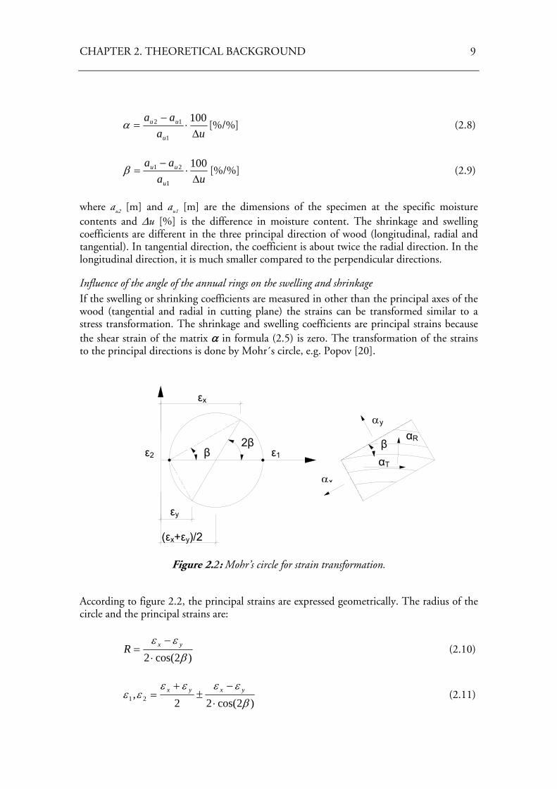
Influence of the angle of the annual rings on the swelling and shrinkage If the swelling or shrinking coefficients are measured in other than the principal axes of the wood (tangential and radial in cutting plane) the strains can be transformed similar to a stress transformation. The shrinkage and swelling coefficients are principal strains because the shear strain of the matrix α in formula (2.5) is zero. The transformation of the strains to the principal directions is done by Mohr´s circle, e.g. Popov [20].
Figure 2.2: Mohr’s circle for strain transformation.
According to figure 2.2, the principal strains are expressed geometrically. The radius of the circle and the principal strains are:
)2cos(2 β
εε⋅
−= yxR (2.10)
)2cos(22
, 21 βεεεε
εε⋅
−±
+= yxyx (2.11)
εx
2β β
βαT
ε1 ε2
(εx+εy)/2
εy
αR
αx
αy
10 CHAPTER 2. THEORETICAL BACKGROUND
The substitution of the strain by the swelling or shrinkage coefficient, respectively, results in the following relations:
)2cos(22 β
ααααα
⋅
−−
+= yxyx
R (2.12)
)2cos(22 β
ααααα
⋅
−+
+= yxyx
T (2.13)
Where αx is the measured strain on the axis closer to the tangential direction and αy the measured strain on the axis perpendicular to α,, see figure 2.2. The chosen sign convention in formula (2.12) and (2.13) is valid if β is in an interval of [-45°;45°].
2.2.4 Mechanical properties of wood
Elastic properties of wood Nine independent constants are needed for the description of the elastic behaviour of an orthotropic material such as wood. These are three moduli of elasticity (EL, ER and ET), three shear moduli (GLT, GLR and GRT) and three Poisson’s ratio (νLR, νLT and νTR). Three dependent constants can else be evaluated from the symmetry condition using the relation between the Poisson’s ratio and the Young’s modulus:
i
ji
j
ij
EEνν
= (2.14)
Hooke’s law For an elastic material, the generalisation of Hooke’s law is described as a law which relates all total strains to the corresponding stress components. Either the strain (ε) can be read as a linear function of the stress (σ) and the inverse of the elastics constants (S) or the stress (σ) as a linear function of the strain (ε) and the elastic constants (C). Thus, the Hooke’s law can be applied to the wood in two forms, e.g. Bodig and Jayne [5]: klijklij S σε ⋅= (2.15)
klijklij C εσ ⋅= (2.16)
The full constants matrix referred to the specific coordinate system of wood (L,T and R) appears as follows for the evaluation of the strain:
CHAPTER 2. THEORETICAL BACKGROUND 11
⎥⎥⎥⎥⎥⎥⎥⎥
⎦
⎤
⎢⎢⎢⎢⎢⎢⎢⎢
⎣
⎡
⋅
⎥⎥⎥⎥⎥⎥⎥⎥⎥⎥⎥⎥⎥⎥⎥
⎦
⎤
⎢⎢⎢⎢⎢⎢⎢⎢⎢⎢⎢⎢⎢⎢⎢
⎣
⎡
−−
−−
−−
=
⎥⎥⎥⎥⎥⎥⎥⎥
⎦
⎤
⎢⎢⎢⎢⎢⎢⎢⎢
⎣
⎡
RT
LT
LR
T
R
L
RT
LT
LR
TR
RT
L
LT
T
TR
RL
LR
T
TL
R
RL
L
RT
LT
LR
T
R
L
G
G
G
EEE
EEE
EEE
τττσσσ
νν
νν
νν
γγγεεε
100000
010000
001000
0001
0001
0001
(2.17)
Where EL, ER and ET [MPa] are the modulus of elasticity in longitudinal, radial and tangential direction, GLR, GLT and GRT [MPa] are the shear moduli, νLT, νLR, νTR, νTL, νRL and νTR are the Poisson’s ratio. The first letter of the subscript refers to direction of applied stress and the second letter to direction of lateral deformation.
Moisture influence on the material properties E moduli, shear moduli and Poisson’s ratios vary within and between species and are affected by moisture content and temperature; see e.g. Ormarsson [16]. If the moisture is higher than the fibre saturation point, FSP, the moisture content is assumed to have no influence on the moduli. However, in the present study, the temperature is assumed to be a constant and the moisture content changes only slightly in the drying and wetting periods. These effects were neglected.
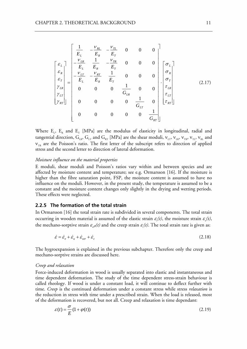
2.2.5 The formation of the total strain In Ormarsson [16] the total strain rate is subdivided in several components. The total strain occurring in wooden material is assumed of the elastic strain εe(t), the moisture strain εu(t), the mechano-sorptive strain εuσ(t) and the creep strain εc(t). The total strain rate is given as: cuue εεεεε σ &&&&& +++= (2.18) The hygroexpansion is explained in the previous subchapter. Therefore only the creep and mechano-sorptive strains are discussed here.
Creep and relaxation Force-induced deformation in wood is usually separated into elastic and instantaneous and time dependent deformation. The study of the time dependent stress-strain behaviour is called rheology. If wood is under a constant load, it will continue to deflect further with time. Creep is the continued deformation under a constant stress while stress relaxation is the reduction in stress with time under a prescribed strain. When the load is released, most of the deformation is recovered, but not all. Creep and relaxation is time dependant:
))(1()( tE
t ϕσε += (2.19)
12 CHAPTER 2. THEORETICAL BACKGROUND
))(1(
)(t
Etϕεσ
+= (2.20)
Were ϕ [-] is the time dependant creep factor in formula (2.19) and the factor of relaxation in formula (2.20). The magnitude of the creep in wood depends on the direction (longitudinal, radial or tangential) and influenced considerably by moistures content, temperature and stress levels. After loading a specimen and the immediate elastic response, the deformation increases with a constant loading. This delayed deformation can in rheological terms be classified as viscoelastic and viscoplastic deformation depending on if these are recoverable after releasing the load, or not. The instantaneous application of load F at time t0 to a wood composite produces an instantaneous elastic deformation ue as shown in figure 2.3. Continuing loading the specimen results in additional deformation called u1 at time t1. After reloading, the elastic part of the deformation ue is recovered directly. A delayed elastic part of the deformation, ude recovers during the flow of the material. The viscoplastic part of the deformation uv does not recover at all and it is permanent.
Forc
e F
Timet t
Defo
rmat
ion u
t t
F
Time
creep recovery
Time
t Time
creep recovery
10
10
flow
permanentinst.eu
u e
u de
vu
u 1
Figure 2.3: Creep curve, load-time and deformation-time function.
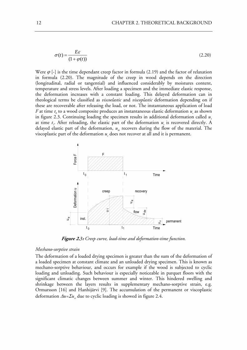
Mechano-sorptive strain The deformation of a loaded drying specimen is greater than the sum of the deformation of a loaded specimen at constant climate and an unloaded drying specimen. This is known as mechano-sorptive behaviour, and occurs for example if the wood is subjected to cyclic loading and unloading. Such behaviour is especially noticeable in parquet floors with the significant climatic changes between summer and winter. This hindered swelling and shrinkage between the layers results in supplementary mechano-sorptive strain, e.g. Ormarsson [16] and Hanhijärvi [9]. The accumulation of the permanent or viscoplastic deformation Δu=Σuvi due to cyclic loading is showed in figure 2.4.
CHAPTER 2. THEORETICAL BACKGROUND 13
1 2 3
u e1
u 1 2u 3u
u e1 u e2 u e3
u
F
t
u
Figure 2.4: Increasing of viscoplastic deformation under cyclic loading.
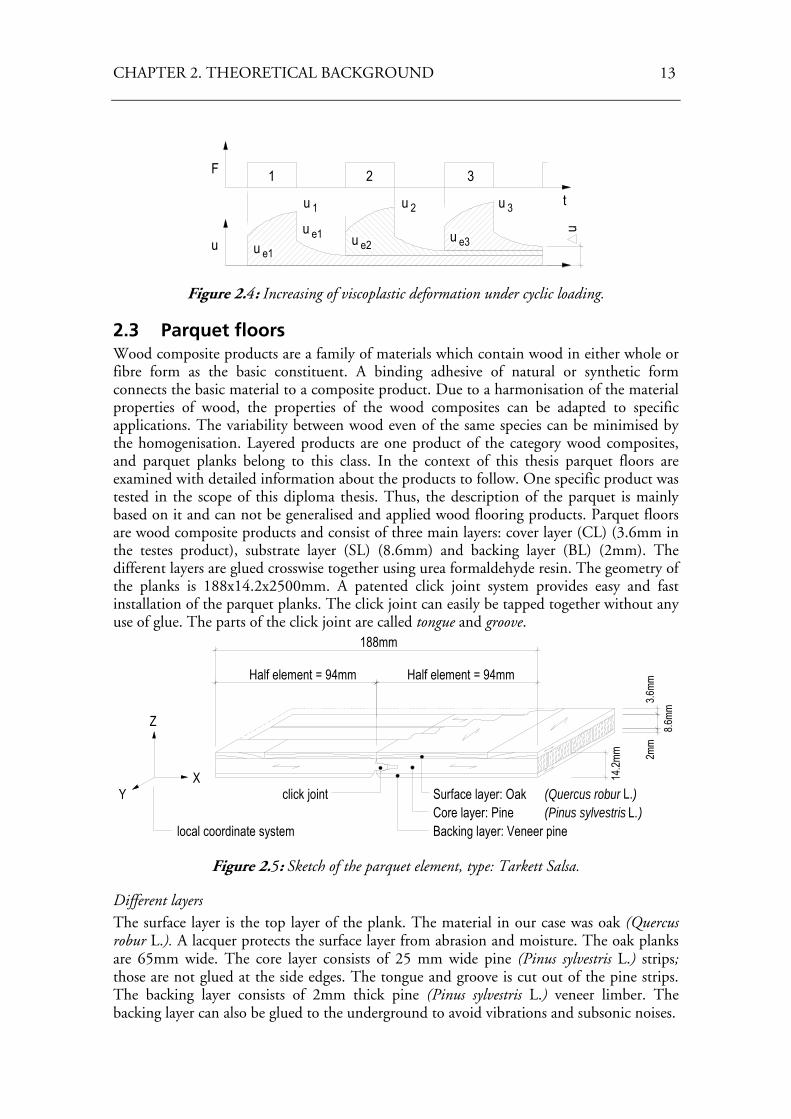
2.3 Parquet floors Wood composite products are a family of materials which contain wood in either whole or fibre form as the basic constituent. A binding adhesive of natural or synthetic form connects the basic material to a composite product. Due to a harmonisation of the material properties of wood, the properties of the wood composites can be adapted to specific applications. The variability between wood even of the same species can be minimised by the homogenisation. Layered products are one product of the category wood composites, and parquet planks belong to this class. In the context of this thesis parquet floors are examined with detailed information about the products to follow. One specific product was tested in the scope of this diploma thesis. Thus, the description of the parquet is mainly based on it and can not be generalised and applied wood flooring products. Parquet floors are wood composite products and consist of three main layers: cover layer (CL) (3.6mm in the testes product), substrate layer (SL) (8.6mm) and backing layer (BL) (2mm). The different layers are glued crosswise together using urea formaldehyde resin. The geometry of the planks is 188x14.2x2500mm. A patented click joint system provides easy and fast installation of the parquet planks. The click joint can easily be tapped together without any use of glue. The parts of the click joint are called tongue and groove.
Half element = 94mm Half element = 94mm
click joint Surface layer: OakCore layer: PineBacking layer: Veneer pine
14.2
mm
(Quercus robur )(Pinus sylvestris )
188mm
X
Z
Y
local coordinate system L.
L.
2mm
8.6m
m3.
6mm
Figure 2.5: Sketch of the parquet element, type: Tarkett Salsa.
Different layers The surface layer is the top layer of the plank. The material in our case was oak (Quercus robur L.). A lacquer protects the surface layer from abrasion and moisture. The oak planks are 65mm wide. The core layer consists of 25 mm wide pine (Pinus sylvestris L.) strips; those are not glued at the side edges. The tongue and groove is cut out of the pine strips. The backing layer consists of 2mm thick pine (Pinus sylvestris L.) veneer limber. The backing layer can also be glued to the underground to avoid vibrations and subsonic noises.
14 CHAPTER 2. THEORETICAL BACKGROUND
UF resin Glues are widely used in joints in wood composite products. Mechanical properties, stability and long term durability are key issues for glued and coated wood. The understanding of the properties and behaviour of the glue line and the wood-glue composite formed at the interface between glue and wood is of considerable importance. The adhesive used for the production of the parquet planks is urea formaldehyde. The temperature of gluing grows up to 90 degrees in a high frequency press. UF resin is mainly used in indoor application because damages in the glue line in a higher humidity range of 90-95% can occur. UF resin is hygroscopic as it contains different flowers, but it is not as hygroscopic as wood, e.g. Blanchet [4]. The exactly composition of the glue is not known. According to Blanchet’s results and the limited knowledge about material properties, the composites glue-wood has been admitted as an elastic interface layer in the model. A parameter study on the long term behaviour of the glue line has been performed in chapter 5 and 6. Residual stresses in parquet planks If the initial moisture content of the basic material before the gluing process differs between the layers and species, residual stresses in the product occur. To minimise the residual stresses the moisture content of each layer in the whole manufacturing process of the planks is strictly controlled by the producer. The guaranteed initial moisture content of the parquet planks until packaging content is in the range of 6.5-7.5%. In the context of this thesis, the residual stresses had not been measured. Thus, those are entered to zero for the calculations. Initial stresses can be measured by slitting up the planks, e.g. Jönsson [14] for example.
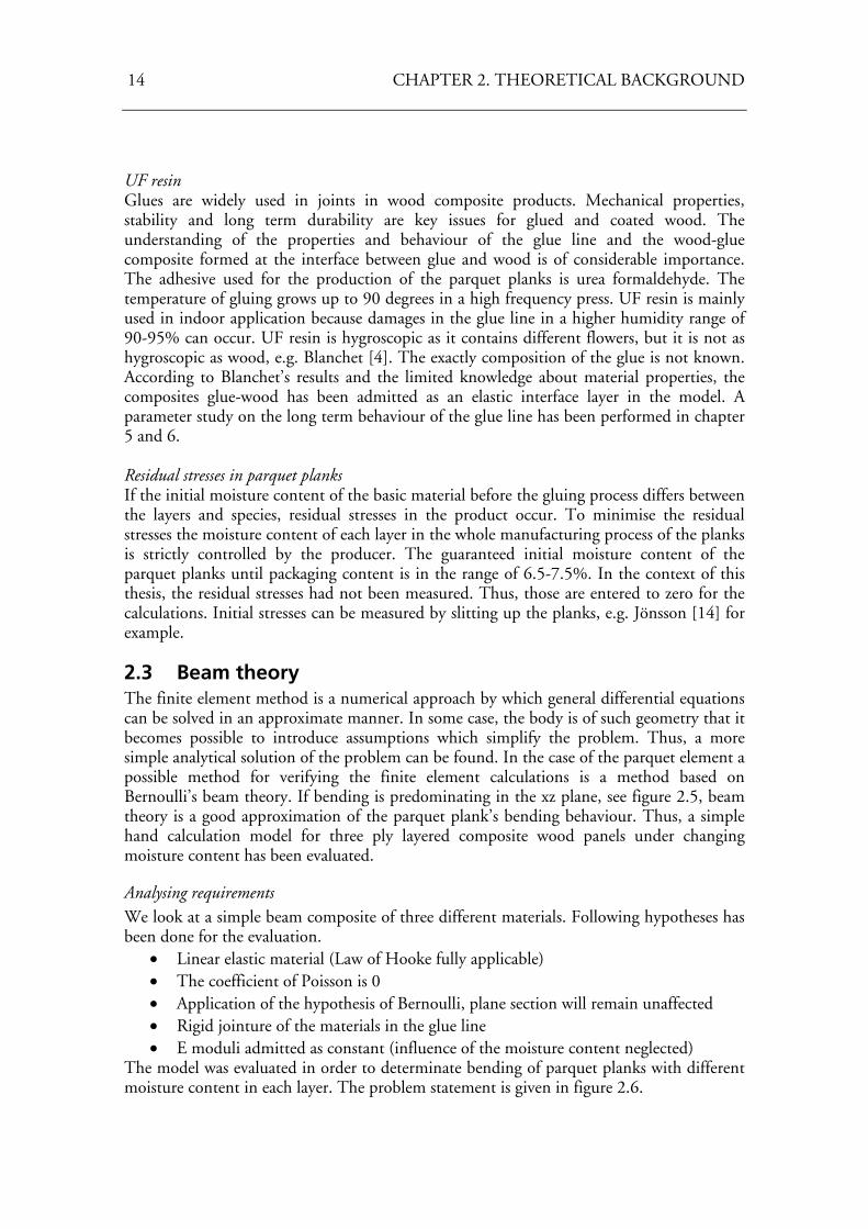
2.3 Beam theory The finite element method is a numerical approach by which general differential equations can be solved in an approximate manner. In some case, the body is of such geometry that it becomes possible to introduce assumptions which simplify the problem. Thus, a more simple analytical solution of the problem can be found. In the case of the parquet element a possible method for verifying the finite element calculations is a method based on Bernoulli’s beam theory. If bending is predominating in the xz plane, see figure 2.5, beam theory is a good approximation of the parquet plank’s bending behaviour. Thus, a simple hand calculation model for three ply layered composite wood panels under changing moisture content has been evaluated.
Analysing requirements We look at a simple beam composite of three different materials. Following hypotheses has been done for the evaluation.
• Linear elastic material (Law of Hooke fully applicable) • The coefficient of Poisson is 0 • Application of the hypothesis of Bernoulli, plane section will remain unaffected • Rigid jointure of the materials in the glue line • E moduli admitted as constant (influence of the moisture content neglected)
The model was evaluated in order to determinate bending of parquet planks with different moisture content in each layer. The problem statement is given in figure 2.6.
CHAPTER 2. THEORETICAL BACKGROUND 15
E
uu
= +
u
uu
u
uu
L
33
3223
2112
11
3
2
1
3
2
1
3 α3d 3
E2 α2
E1 α1
d 2
d 1
Δ
ΔΔ
uuu
u
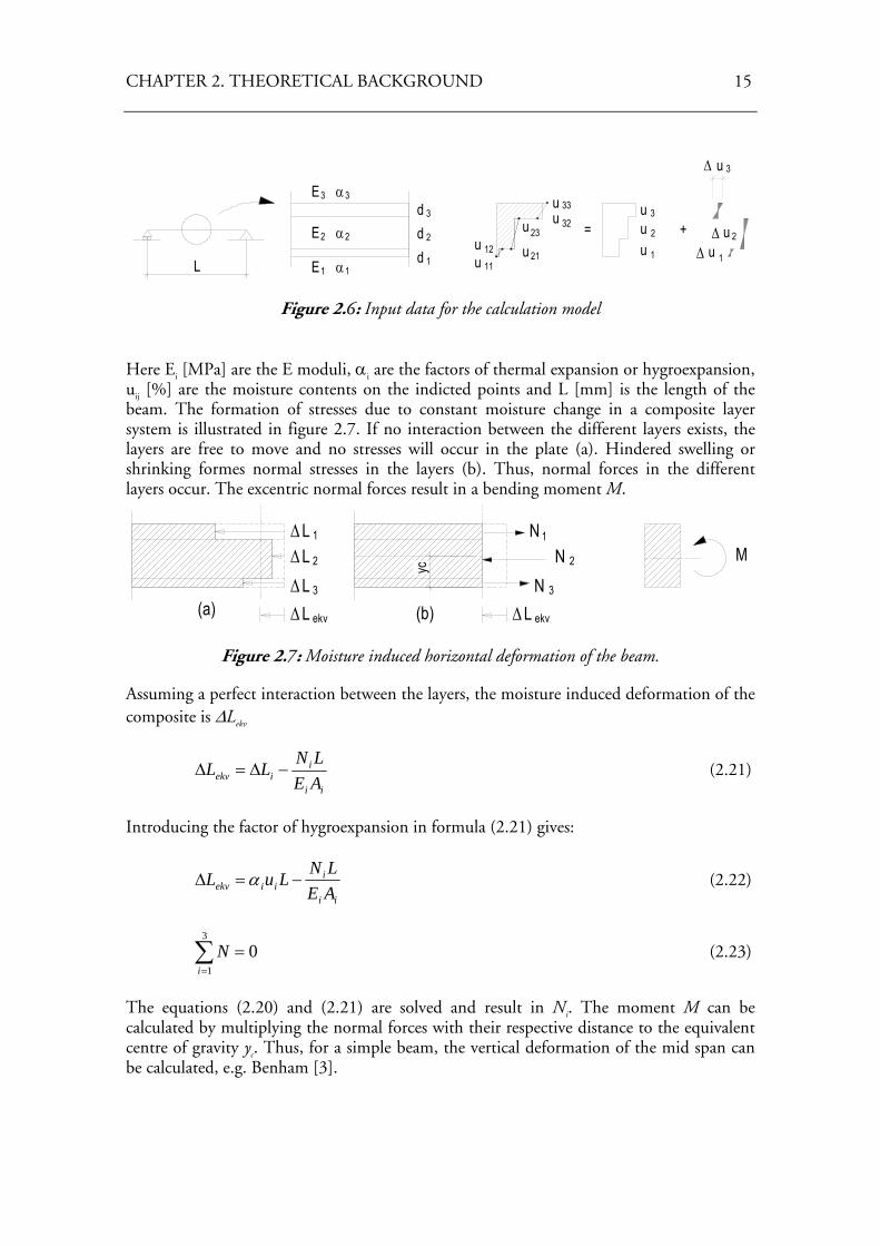
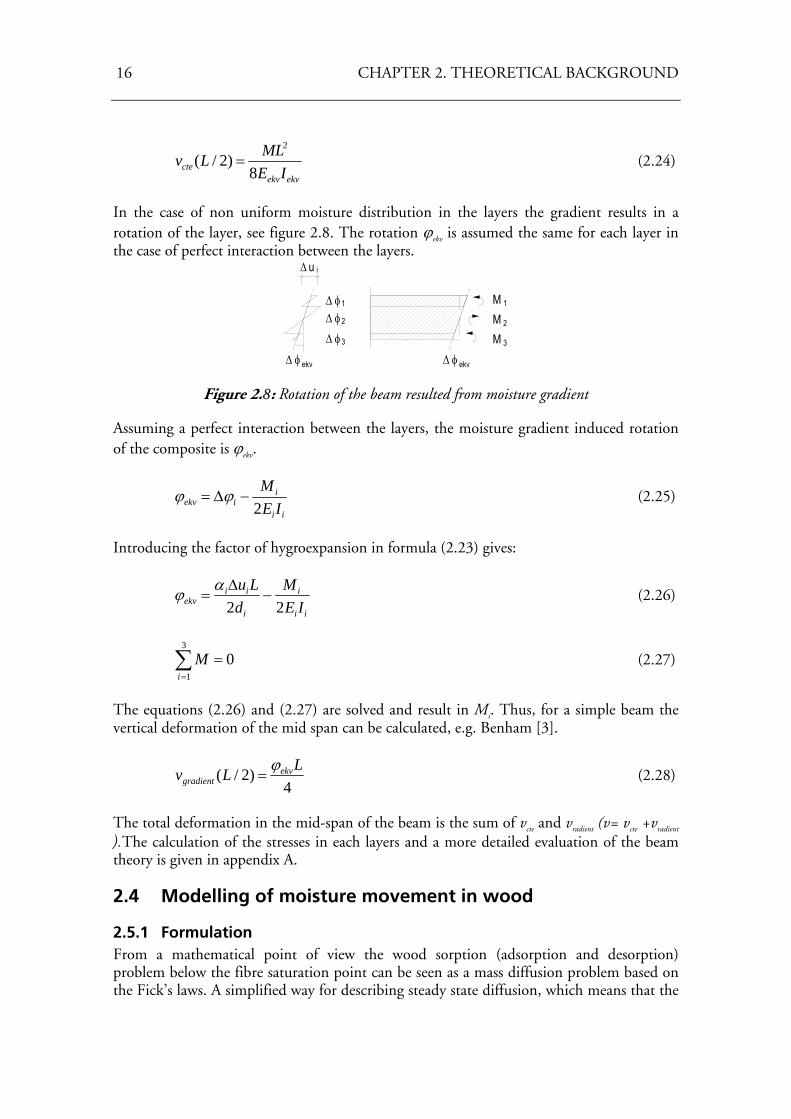
Figure 2.6: Input data for the calculation model
Here Ei [MPa] are the E moduli, αi are the factors of thermal expansion or hygroexpansion, uij [%] are the moisture contents on the indicted points and L [mm] is the length of the beam. The formation of stresses due to constant moisture change in a composite layer system is illustrated in figure 2.7. If no interaction between the different layers exists, the layers are free to move and no stresses will occur in the plate (a). Hindered swelling or shrinking formes normal stresses in the layers (b). Thus, normal forces in the different layers occur. The excentric normal forces result in a bending moment M.
L 1ΔL 2Δ
L 3ΔL ekvΔ
NN 2
N 3
L ekvΔ
M
yc
1
(a) (b)
Figure 2.7: Moisture induced horizontal deformation of the beam.
Assuming a perfect interaction between the layers, the moisture induced deformation of the composite is ΔLekv
ii
iiekv AE
LNLL −Δ=Δ (2.21)
Introducing the factor of hygroexpansion in formula (2.21) gives:
ii
iiiekv AE
LNLuL −=Δ α (2.22)
∑=
=3
10
iN (2.23)
The equations (2.20) and (2.21) are solved and result in Ni. The moment M can be calculated by multiplying the normal forces with their respective distance to the equivalent centre of gravity yc. Thus, for a simple beam, the vertical deformation of the mid span can be calculated, e.g. Benham [3].
16 CHAPTER 2. THEORETICAL BACKGROUND
ekvekv
cte IEMLLv
8)2/(
2
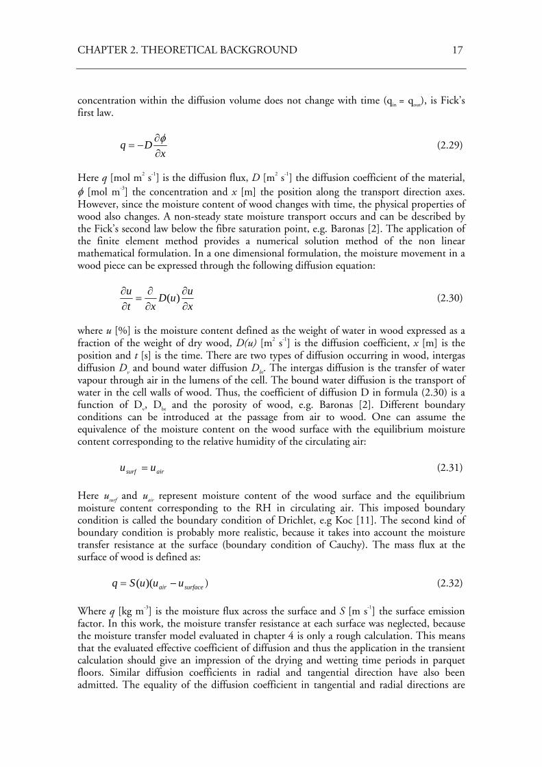
= (2.24)
In the case of non uniform moisture distribution in the layers the gradient results in a rotation of the layer, see figure 2.8. The rotation ϕekv is assumed the same for each layer in the case of perfect interaction between the layers.
1Δ φ2Δ φ
3Δ φ
Δ φ ekv
u iΔ
Δ φ ekv
M 1
M 2
M 3
Figure 2.8: Rotation of the beam resulted from moisture gradient
Assuming a perfect interaction between the layers, the moisture gradient induced rotation of the composite is ϕekv.
ii
iiekv IE
M2
−Δ= ϕϕ (2.25)
Introducing the factor of hygroexpansion in formula (2.23) gives:
ii
i
i
iiekv IE
Md
Lu22
−Δ
=αϕ (2.26)
∑=
=3
1
0i
M (2.27)
The equations (2.26) and (2.27) are solved and result in Mi. Thus, for a simple beam the vertical deformation of the mid span can be calculated, e.g. Benham [3].
4
)2/( LLv ekvgradient
ϕ= (2.28)
The total deformation in the mid-span of the beam is the sum of vcte and vradient (v= vcte +vradient
).The calculation of the stresses in each layers and a more detailed evaluation of the beam theory is given in appendix A.
2.4 Modelling of moisture movement in wood
2.5.1 Formulation From a mathematical point of view the wood sorption (adsorption and desorption) problem below the fibre saturation point can be seen as a mass diffusion problem based on the Fick’s laws. A simplified way for describing steady state diffusion, which means that the
CHAPTER 2. THEORETICAL BACKGROUND 17
concentration within the diffusion volume does not change with time (qin = qout), is Fick’s first law.
x
Dq∂∂
−=φ
(2.29)
Here q [mol m2 s-1] is the diffusion flux, D [m2 s-1] the diffusion coefficient of the material, φ [mol m-3] the concentration and x [m] the position along the transport direction axes. However, since the moisture content of wood changes with time, the physical properties of wood also changes. A non-steady state moisture transport occurs and can be described by the Fick’s second law below the fibre saturation point, e.g. Baronas [2]. The application of the finite element method provides a numerical solution method of the non linear mathematical formulation. In a one dimensional formulation, the moisture movement in a wood piece can be expressed through the following diffusion equation:
xuuD
xtu
∂∂
∂∂
=∂∂ )( (2.30)
where u [%] is the moisture content defined as the weight of water in wood expressed as a fraction of the weight of dry wood, D(u) [m2 s-1] is the diffusion coefficient, x [m] is the position and t [s] is the time. There are two types of diffusion occurring in wood, intergas diffusion Dv and bound water diffusion Dbt. The intergas diffusion is the transfer of water vapour through air in the lumens of the cell. The bound water diffusion is the transport of water in the cell walls of wood. Thus, the coefficient of diffusion D in formula (2.30) is a function of Dv, Dbt and the porosity of wood, e.g. Baronas [2]. Different boundary conditions can be introduced at the passage from air to wood. One can assume the equivalence of the moisture content on the wood surface with the equilibrium moisture content corresponding to the relative humidity of the circulating air: airsurf uu = (2.31)
Here usurf and uair represent moisture content of the wood surface and the equilibrium moisture content corresponding to the RH in circulating air. This imposed boundary condition is called the boundary condition of Drichlet, e.g Koc [11]. The second kind of boundary condition is probably more realistic, because it takes into account the moisture transfer resistance at the surface (boundary condition of Cauchy). The mass flux at the surface of wood is defined as:
surfaceair uuuSq −= )(( ) (2.32)
Where q [kg m-3] is the moisture flux across the surface and S [m s-1] the surface emission factor. In this work, the moisture transfer resistance at each surface was neglected, because the moisture transfer model evaluated in chapter 4 is only a rough calculation. This means that the evaluated effective coefficient of diffusion and thus the application in the transient calculation should give an impression of the drying and wetting time periods in parquet floors. Similar diffusion coefficients in radial and tangential direction have also been admitted. The equality of the diffusion coefficient in tangential and radial directions are
18 CHAPTER 2. THEORETICAL BACKGROUND
satisfied until 15% moisture content see Jönsson [14] and Koponen [11]. The diffusion coefficient in the longitudinal direction is larger than in tangential and radial directions. However the moisture distribution has been calculated in one dimension and the diffusion coefficient in the longitudinal (direction of the grain) has not been used in the scope of this diploma thesis.
2.5.2 Similarity of the moisture transport to a temperature field The moisture content for each step of the calculation has been calculated using the analogy of a temperature field to a mass transport field. A temperature field and the deformation can be easily coupled together in ABAQUS. The differential equation describes a one dimensional temperature field:
⎟⎠⎞
⎜⎝⎛
∂∂
∂∂
=∂∂
xTT
xtTc )(λρ (2.33)
Here T [deg] is the temperature, c [J kg-1K-1] is the specific heat, ρ [kg/m3] is the density and λ is the thermal conductivity [J s-1m-1K-1]. Dividing the equation by c and ρ results in the expression as follows:
⎟⎟⎠
⎞⎜⎜⎝
⎛∂∂
∂∂
=∂∂
xT
cT
xtT
ρλ )(
(2.34)
The moisture transport can be simulated by substitution of the variables from the temperature field. The diffusion coefficient of wood Dw [m
2 s-1] replaces the specific heat, density and thermal conductivity of the temperature field in formula (2.34). The new formula describes the one dimensional moisture transport in a solid material:
⎟⎠⎞
⎜⎝⎛
∂∂
∂∂
=∂∂
xuuD
xtu
W )( (2.35)
The formula is similar to formula (2.30) where u [%] is the moisture content of wood dependant on time and position and Dw [m
2 s-1] is the effective coefficient of diffusion. The setting of the density and the specific heat to 1 in ABAQUS allows calculation of the moisture induced deformation at each time t. The method of calculation has been tested and compared to the analytical solution for a semi infinitive body, e.g. Carslaw [6]:
002),( uu
tDxerfxtu
w
+⎟⎟⎠
⎞⎜⎜⎝
⎛= (2.36)
Here erf(x) is the error function, u0 [%] is the moisture of the expanded surface at time t and x [m] is the distance of the calculated moisture content to the expanded surface.
19
Chapter 3
Experimental tests
3.1 Introduction The aim of this chapter is to present the experimental results including the measurements performed at the Swiss Federal Institute of Technology in Zurich (autumn 2005) and at Lund University (winter 2005-2006). The following subdivision of the test series has been done. The first part concerned experiments on basic materials, used for the production of the parquet planks type Tarkett Salsa. Two different species, namely pine (Pinus sylvestris L.) and oak wood (Quercus robur L.), were tested in the context of this diploma thesis. The measurements included sorptional behaviour, hygroexpansion under changing climate and the determination of the static E-modulus parallel to the grain direction by standardised three point bending test. The second part of the experiments dealt with measurements of the deformational behaviour of parquet elements under different climatic conditions. The results should provide data for calibrating the finite element model in the following chapters. Additional measurements in alternating conditions have been conducted for simulating the mechano-sorptional behaviour of wood composite products.
3.2 Tests on basic material
3.2.1 Sorptional behaviour and density
Materials and methods Pine (Pinus sylvestris L.) and oak (Querqus robur L.) samples were cut from the delivered material with the geometry according to table 3.1. First, the samples from each species were conditioned in a climatic chamber of 20° degrees and 35% relative humidity (RH) until they reached equilibrium moisture content (EMC). The behaviour of sorption has been measured after changing climate going from 35% to over 50% and up to 85% relative humidity, all at a temperature of 20° Celsius. The climate was changed after the specimens reached moisture equilibrium content with the surrounding air. In addition to the weight, the density has been determined and recorded by measuring the dimensions at the standard climate of 20°/65%. These tests were performed at the Swiss Federal Institute of Technology in Zurich in autumn 2005. Because a more powerful climatic chamber was available in Lund, a second test series with different samples of the same specimens and consignment were performed at the Lund University winter 2005/2006. Refining the sorptional curve was the main reason for providing a second test series. The specimens were conditioned at a climate of 20°/25% relative humidity. The weight was measured after the
20 CHAPTER 3. EXPERIMENTAL TESTS
test specimens reached equilibrium moisture content in climates of 25% and 95% relative humidity respectively, all at a temperature of 20°C. This supplementary tests series provided more values for fitting the adsorption curve. Detailed results of the measurements are listed in the appendix B, table B1.
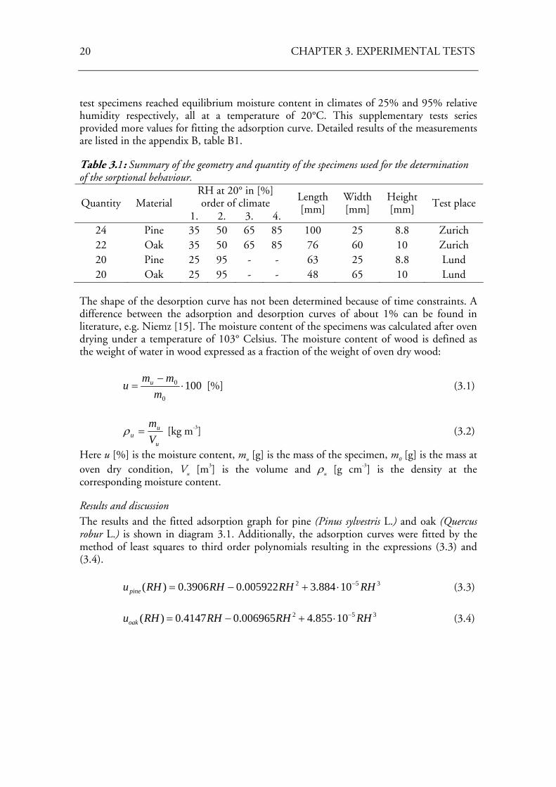
Table 3.1: Summary of the geometry and quantity of the specimens used for the determination of the sorptional behaviour.
RH at 20° in [%] order of climate Quantity Material
1. 2. 3. 4.
Length [mm]
Width [mm]
Height [mm] Test place
24 Pine 35 50 65 85 100 25 8.8 Zurich 22 Oak 35 50 65 85 76 60 10 Zurich 20 Pine 25 95 - - 63 25 8.8 Lund 20 Oak 25 95 - - 48 65 10 Lund
The shape of the desorption curve has not been determined because of time constraints. A difference between the adsorption and desorption curves of about 1% can be found in literature, e.g. Niemz [15]. The moisture content of the specimens was calculated after oven drying under a temperature of 103° Celsius. The moisture content of wood is defined as the weight of water in wood expressed as a fraction of the weight of oven dry wood:
1000
0 ⋅−
=m
mmu u [%] (3.1)
u
uu V
m=ρ [kg m-3] (3.2)
Here u [%] is the moisture content, mu [g] is the mass of the specimen, m0 [g] is the mass at oven dry condition, Vu [m3] is the volume and ρu [g cm-3] is the density at the corresponding moisture content.
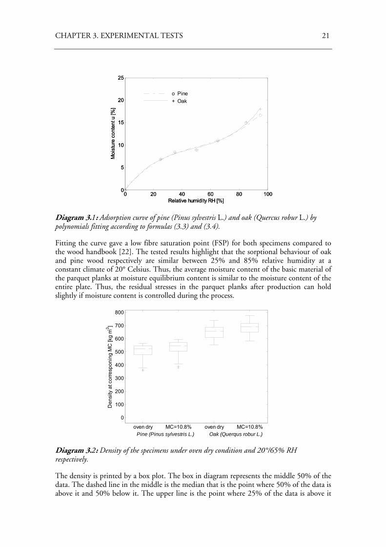
Results and discussion The results and the fitted adsorption graph for pine (Pinus sylvestris L.) and oak (Quercus robur L.) is shown in diagram 3.1. Additionally, the adsorption curves were fitted by the method of least squares to third order polynomials resulting in the expressions (3.3) and (3.4). 352 10884.3005922.03906.0)( RHRHRHRHupine
−⋅+−= (3.3)
352 10855.4006965.04147.0)( RHRHRHRHuoak
−⋅+−= (3.4)
CHAPTER 3. EXPERIMENTAL TESTS 21
0 20 40 60 80 1000
5
10
15
20
25
Relative humidity RH [%]
Moi
stur
e co
nten
t u [%
]
o Pine + Oak
0 20 40 60 80 1000
5
10
15
20
25
Relative humidity RH [%]
Moi
stur
e co
nten
t u [%
]
o Pine + Oak
Diagram 3.1: Adsorption curve of pine (Pinus sylvestris L.) and oak (Quercus robur L.) by polynomials fitting according to formulas (3.3) and (3.4).
Fitting the curve gave a low fibre saturation point (FSP) for both specimens compared to the wood handbook [22]. The tested results highlight that the sorptional behaviour of oak and pine wood respectively are similar between 25% and 85% relative humidity at a constant climate of 20° Celsius. Thus, the average moisture content of the basic material of the parquet planks at moisture equilibrium content is similar to the moisture content of the entire plate. Thus, the residual stresses in the parquet planks after production can hold slightly if moisture content is controlled during the process.
oven dry MC=10.8% oven dry MC=10.8%
0
100
200
300
400
500
600
700
800
Den
sity
at c
orre
spon
ing
MC
[kg
m-3]
Pine (Pinus sylvestris L.) Oak (Querqus robur L.)
Diagram 3.2: Density of the specimens under oven dry condition and 20°/65% RH respectively.
The density is printed by a box plot. The box in diagram represents the middle 50% of the data. The dashed line in the middle is the median that is the point where 50% of the data is above it and 50% below it. The upper line is the point where 25% of the data is above it
22 CHAPTER 3. EXPERIMENTAL TESTS
and the lower edge of the box where 25% of the data fall below it. The mean values for pine wood where ρ0 = 495 [kg m-3] and ρ10.8 = 522 [kg m-3] and for oak ρ0 = 660 [kg m-3] and ρ10.8 = 694 [kg m-3]. The obtained values are similar to literature values, e.g. Niemz [15].
3.2.2 E-Modulus
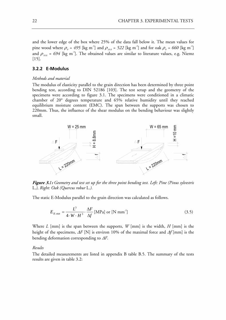
Methods and material The modulus of elasticity parallel to the grain direction has been determined by three point bending test, according to DIN 52186 [103]. The test setup and the geometry of the specimens were according to figure 3.1. The specimens were conditioned in a climatic chamber of 20° degrees temperature and 65% relative humidity until they reached equilibrium moisture content (EMC). The span between the supports was chosen to 220mm. Thus, the influence of the shear modulus on the bending behaviour was slightly small.
L = 220mm
f
W = 25 mm
F
H =
8.8m
m
F H =1
0 mm
L = 220mm
f
W = 65 mm
Figure 3.1: Geometry and test set up for the three point bending test. Left: Pine (Pinus sylvestris L.), Right: Oak (Quercus robur L.).
The static E-Modulus parallel to the grain direction was calculated as follows.
fF
HWLE statII Δ
Δ⋅
⋅⋅= 3
3
. 4[MPa] or [N mm-2] (3.5)
Where L [mm] is the span between the supports, W [mm] is the width, H [mm] is the height of the specimens, ΔF [N] is environ 10% of the maximal force and Δf [mm] is the bending deformation corresponding to ΔF.
Results The detailed measurements are listed in appendix B table B.5. The summary of the tests results are given in table 3.2:
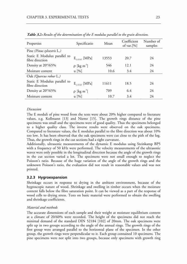
CHAPTER 3. EXPERIMENTAL TESTS 23
Table 3.2: Results of the determination of the E modulus parallel to the grain direction.
Properties Specificatio Mean Coefficient of var.[%]
Number of samples
Pine (Pinus sylvestris L.) Static E Modulus parallel to fibre direction EL.STAT [MPa] 13553 20.7 24
Density at 20°/65% ρ [kg m-3] 546 12.1 24
Moisture content u [%] 10.6 3.4 24 Oak (Quercus robur L.) Static E Modulus parallel to fibre direction EL.STAT [MPa] 11611 18.5 24
Density at 20°/65% ρ [kg m-3] 709 6.4 24
Moisture content u [%] 10.7 3.4 24
Discussion The E moduli of pine wood from the tests were about 20% higher compared to literature values, e.g. Kollmann [13] and Niemz [15]. The growth rings distance of the pine specimens was small and the specimens were of good quality. Thus the specimens belonged to a higher quality class. The inverse results were observed on the oak specimens. Compared to literature values, the E modulus parallel to the fibre direction was about 10% too low. It has been observed that the oak specimens were cut close to the pith of the log. Thus, the growth rings in the cut sections had a tight curvature. Additionally, ultrasonic measurements of the dynamic E modulus using Steinkamp BP5 with a frequency of 50 kHz were performed. The velocity measurements of the ultrasonic waves were only possible in the longitudinal direction because the angle of the growth rings in the cut section varied a lot. The specimens were not small enough to neglect the Poisson’s ratio. Because of the huge variation of the angle of the growth rings and the unknown Poisson’s ratio, the evaluation did not result in reasonable values and was not printed.
3.2.3 Hygroexpansion Shrinkage occurs in response to drying in the ambient environment, because of the hygroscopic nature of wood. Shrinkage and swelling in timber occurs when the moisture content falls below the fibre saturation point. It can be viewed as a part of the response of wood cells to drying stress. Tests on basic material were performed to obtain the swelling and shrinkage coefficients.
Material and methods The accurate dimensions of each sample and their weight at moisture equilibrium content at a climate of 20/60% were recorded. The height of the specimens did not reach the minimal demand of the standard DIN 52184 [102] of 20mm. The oak specimens were split up in two groups according to the angle of the annual rings. The growth rings of the first group were arranged parallel to the horizontal plane of the specimen. In the other group, the growth rings were perpendicular to it. Each group contained 10 specimens. The pine specimens were not split into two groups, because only specimens with growth ring
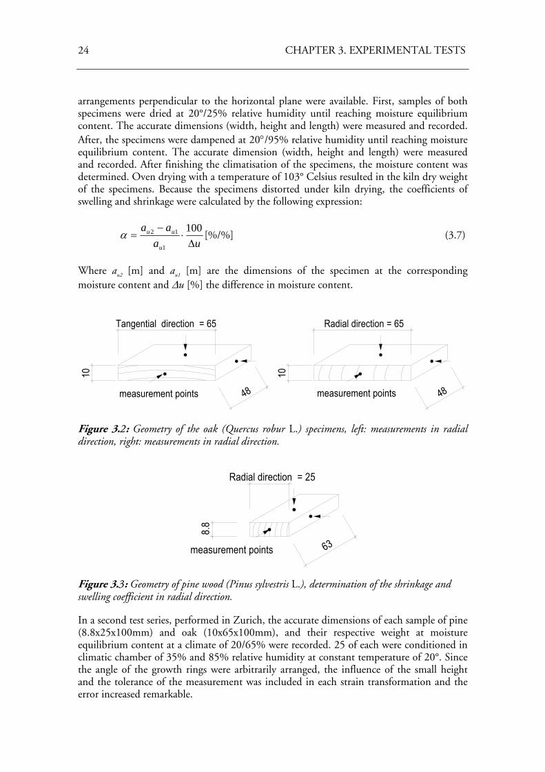
24 CHAPTER 3. EXPERIMENTAL TESTS
arrangements perpendicular to the horizontal plane were available. First, samples of both specimens were dried at 20°/25% relative humidity until reaching moisture equilibrium content. The accurate dimensions (width, height and length) were measured and recorded. After, the specimens were dampened at 20°/95% relative humidity until reaching moisture equilibrium content. The accurate dimension (width, height and length) were measured and recorded. After finishing the climatisation of the specimens, the moisture content was determined. Oven drying with a temperature of 103° Celsius resulted in the kiln dry weight of the specimens. Because the specimens distorted under kiln drying, the coefficients of swelling and shrinkage were calculated by the following expression:
ua
aa
u
uu
Δ⋅
−=
100
1
12α [%/%] (3.7)
Where au2 [m] and au1 [m] are the dimensions of the specimen at the corresponding moisture content and Δu [%] the difference in moisture content.
10
Tangential direction = 65
48
10
Radial direction = 65
48measurement points measurement points
Figure 3.2: Geometry of the oak (Quercus robur L.) specimens, left: measurements in radial direction, right: measurements in radial direction.
measurement points
8.8
Radial direction = 25
63
Figure 3.3: Geometry of pine wood (Pinus sylvestris L.), determination of the shrinkage and swelling coefficient in radial direction.
In a second test series, performed in Zurich, the accurate dimensions of each sample of pine (8.8x25x100mm) and oak (10x65x100mm), and their respective weight at moisture equilibrium content at a climate of 20/65% were recorded. 25 of each were conditioned in climatic chamber of 35% and 85% relative humidity at constant temperature of 20°. Since the angle of the growth rings were arbitrarily arranged, the influence of the small height and the tolerance of the measurement was included in each strain transformation and the error increased remarkable.
CHAPTER 3. EXPERIMENTAL TESTS 25
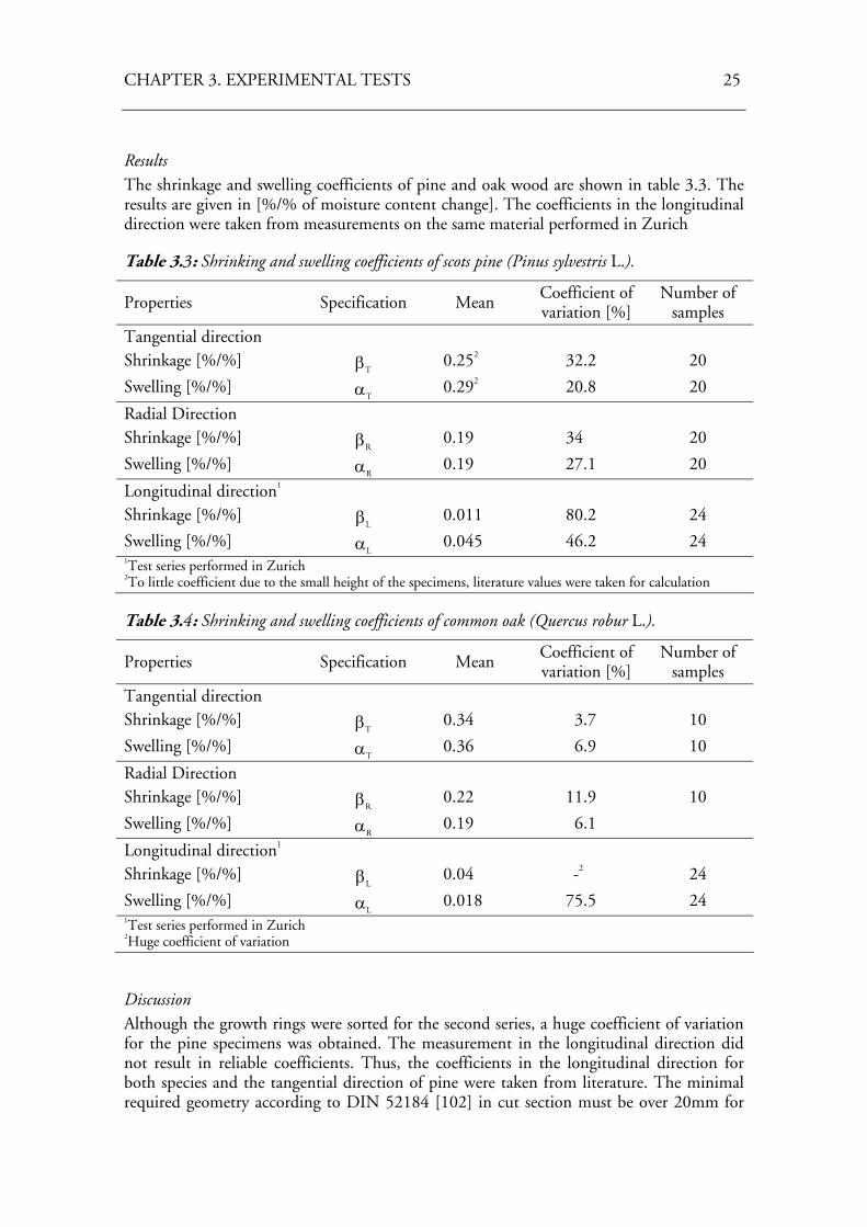
Results The shrinkage and swelling coefficients of pine and oak wood are shown in table 3.3. The results are given in [%/% of moisture content change]. The coefficients in the longitudinal direction were taken from measurements on the same material performed in Zurich
Table 3.3: Shrinking and swelling coefficients of scots pine (Pinus sylvestris L.).
Properties Specification Mean Coefficient of variation [%]
Number of samples
Tangential direction Shrinkage [%/%] βT
0.252 32.2 20
Swelling [%/%] αT 0.292 20.8 20
Radial Direction Shrinkage [%/%] βR
0.19 34 20
Swelling [%/%] αR 0.19 27.1 20
Longitudinal direction1 Shrinkage [%/%] βL
0.011 80.2 24
Swelling [%/%] αL 0.045 46.2 24 1Test series performed in Zurich 2To little coefficient due to the small height of the specimens, literature values were taken for calculation
Table 3.4: Shrinking and swelling coefficients of common oak (Quercus robur L.).
Properties Specification Mean Coefficient of variation [%]
Number of samples
Tangential direction Shrinkage [%/%] βT
0.34 3.7 10
Swelling [%/%] αT 0.36 6.9 10
Radial Direction Shrinkage [%/%] βR
0.22 11.9 10
Swelling [%/%] αR 0.19 6.1
Longitudinal direction1 Shrinkage [%/%] βL
0.04 -2 24
Swelling [%/%] αL 0.018 75.5 24 1Test series performed in Zurich 2Huge coefficient of variation
Discussion Although the growth rings were sorted for the second series, a huge coefficient of variation for the pine specimens was obtained. The measurement in the longitudinal direction did not result in reliable coefficients. Thus, the coefficients in the longitudinal direction for both species and the tangential direction of pine were taken from literature. The minimal required geometry according to DIN 52184 [102] in cut section must be over 20mm for
26 CHAPTER 3. EXPERIMENTAL TESTS
obtaining better results. In longitudinal direction, 100mm was also insufficient for getting reliable results. The problem with longer specimens is the time required for acclimatisation.
3.3 Tests on 150x150mm parquet squares The calibration of the finite element model in the following chapters, tests on wood composites products (parquet planks in our case) have been conducted in Zurich and Lund.
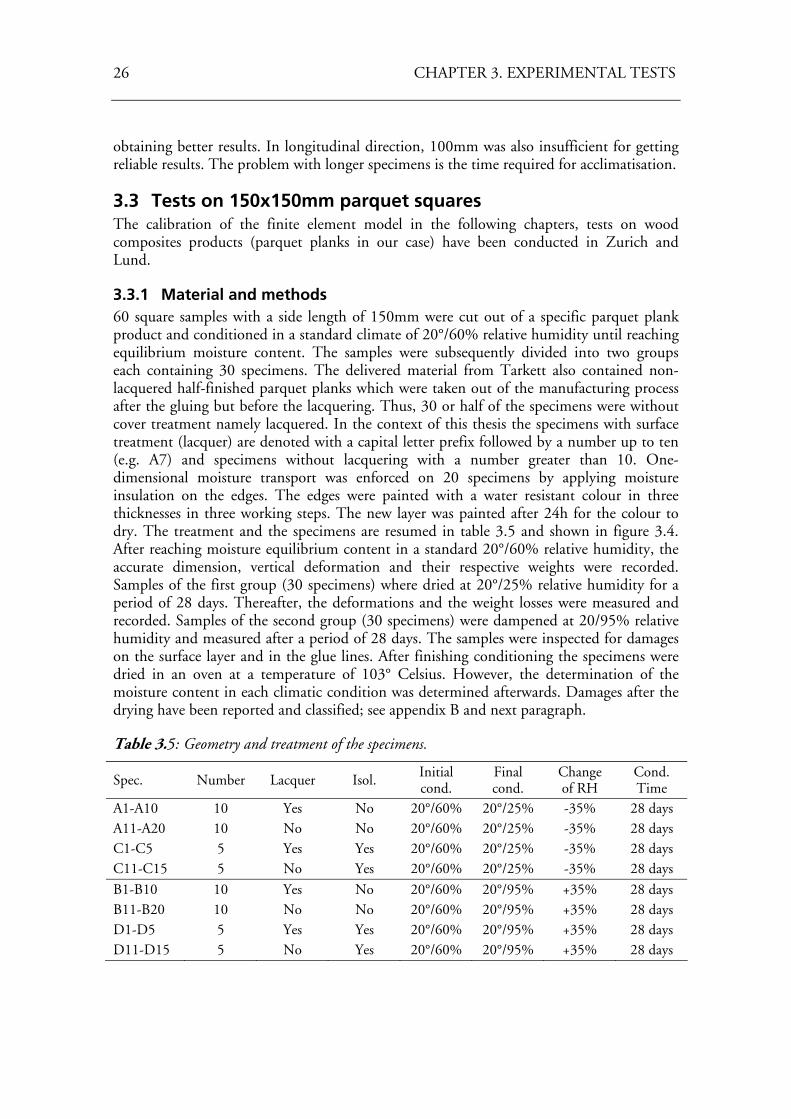
3.3.1 Material and methods 60 square samples with a side length of 150mm were cut out of a specific parquet plank product and conditioned in a standard climate of 20°/60% relative humidity until reaching equilibrium moisture content. The samples were subsequently divided into two groups each containing 30 specimens. The delivered material from Tarkett also contained non-lacquered half-finished parquet planks which were taken out of the manufacturing process after the gluing but before the lacquering. Thus, 30 or half of the specimens were without cover treatment namely lacquered. In the context of this thesis the specimens with surface treatment (lacquer) are denoted with a capital letter prefix followed by a number up to ten (e.g. A7) and specimens without lacquering with a number greater than 10. One-dimensional moisture transport was enforced on 20 specimens by applying moisture insulation on the edges. The edges were painted with a water resistant colour in three thicknesses in three working steps. The new layer was painted after 24h for the colour to dry. The treatment and the specimens are resumed in table 3.5 and shown in figure 3.4. After reaching moisture equilibrium content in a standard 20°/60% relative humidity, the accurate dimension, vertical deformation and their respective weights were recorded. Samples of the first group (30 specimens) where dried at 20°/25% relative humidity for a period of 28 days. Thereafter, the deformations and the weight losses were measured and recorded. Samples of the second group (30 specimens) were dampened at 20/95% relative humidity and measured after a period of 28 days. The samples were inspected for damages on the surface layer and in the glue lines. After finishing conditioning the specimens were dried in an oven at a temperature of 103° Celsius. However, the determination of the moisture content in each climatic condition was determined afterwards. Damages after the drying have been reported and classified; see appendix B and next paragraph.
Table 3.5: Geometry and treatment of the specimens.
Spec. Number Lacquer Isol. Initial cond.
Final cond.
Change of RH
Cond. Time
A1-A10 10 Yes No 20°/60% 20°/25% -35% 28 days A11-A20 10 No No 20°/60% 20°/25% -35% 28 days C1-C5 5 Yes Yes 20°/60% 20°/25% -35% 28 days C11-C15 5 No Yes 20°/60% 20°/25% -35% 28 days
B1-B10 10 Yes No 20°/60% 20°/95% +35% 28 days B11-B20 10 No No 20°/60% 20°/95% +35% 28 days D1-D5 5 Yes Yes 20°/60% 20°/95% +35% 28 days D11-D15 5 No Yes 20°/60% 20°/95% +35% 28 days
CHAPTER 3. EXPERIMENTAL TESTS 27
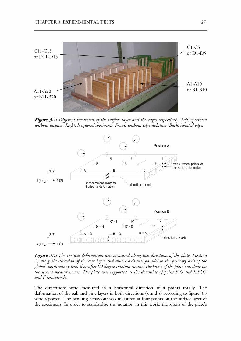
Figure 3.4: Different treatment of the surface layer and the edges respectively. Left: specimen without lacquer. Right: lacquered specimens. Front: without edge isolation. Back: isolated edges.
3 (Y) 1 (X)
2 (Z)
A' = G B' = D C' = A
D' = H E' = E F' = BH'G' = I I'=C
3 (X) 1 (Y)
2 (Z)
A B C
D E FHG I
Position B
Position A
measurement points for horizontal deformation
horizontal deformationmeasurement points for direction of x axis
direction of x axis
Figure 3.5: The vertical deformation was measured along two directions of the plate, Position A, the grain direction of the core layer and thus x axis was parallel to the primary axis of the global coordinate system, thereafter 90 degree rotation counter clockwise of the plate was done for the second measurements. The plate was supported at the downside of point B,G and I.,B’,G’ and I’ respectively.
The dimensions were measured in a horizontal direction at 4 points totally. The deformation of the oak and pine layers in both directions (x and z) according to figure 3.5 were reported. The bending behaviour was measured at four points on the surface layer of the specimens. In order to standardise the notation in this work, the x axis of the plate’s
C1-C5or D1-D5
A1-A10or B1-B10
C11-C15 or D11-D15
A11-A20 or B11-B20
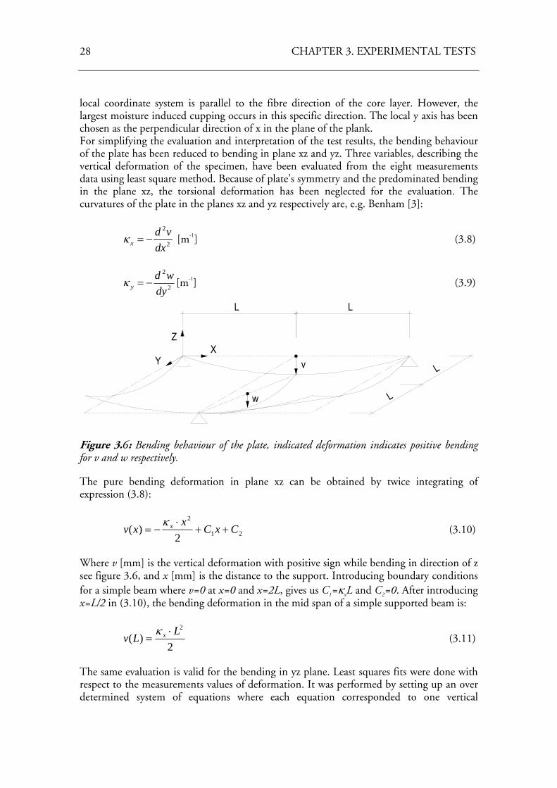
28 CHAPTER 3. EXPERIMENTAL TESTS
local coordinate system is parallel to the fibre direction of the core layer. However, the largest moisture induced cupping occurs in this specific direction. The local y axis has been chosen as the perpendicular direction of x in the plane of the plank. For simplifying the evaluation and interpretation of the test results, the bending behaviour of the plate has been reduced to bending in plane xz and yz. Three variables, describing the vertical deformation of the specimen, have been evaluated from the eight measurements data using least square method. Because of plate’s symmetry and the predominated bending in the plane xz, the torsional deformation has been neglected for the evaluation. The curvatures of the plate in the planes xz and yz respectively are, e.g. Benham [3]:
2
2
dxvd
x −=κ [m-1] (3.8)
2
2
dywd
y −=κ [m-1] (3.9)
w
YX
Z
L L
L
Lv
Figure 3.6: Bending behaviour of the plate, indicated deformation indicates positive bending for v and w respectively.
The pure bending deformation in plane xz can be obtained by twice integrating of expression (3.8):
21
2
2)( CxC
xxv x ++
⋅−=
κ (3.10)
Where v [mm] is the vertical deformation with positive sign while bending in direction of z see figure 3.6, and x [mm] is the distance to the support. Introducing boundary conditions for a simple beam where v=0 at x=0 and x=2L, gives us C1=κxL and C2=0. After introducing x=L/2 in (3.10), the bending deformation in the mid span of a simple supported beam is:
2
)(2LLv x ⋅
=κ
(3.11)
The same evaluation is valid for the bending in yz plane. Least squares fits were done with respect to the measurements values of deformation. It was performed by setting up an over determined system of equations where each equation corresponded to one vertical
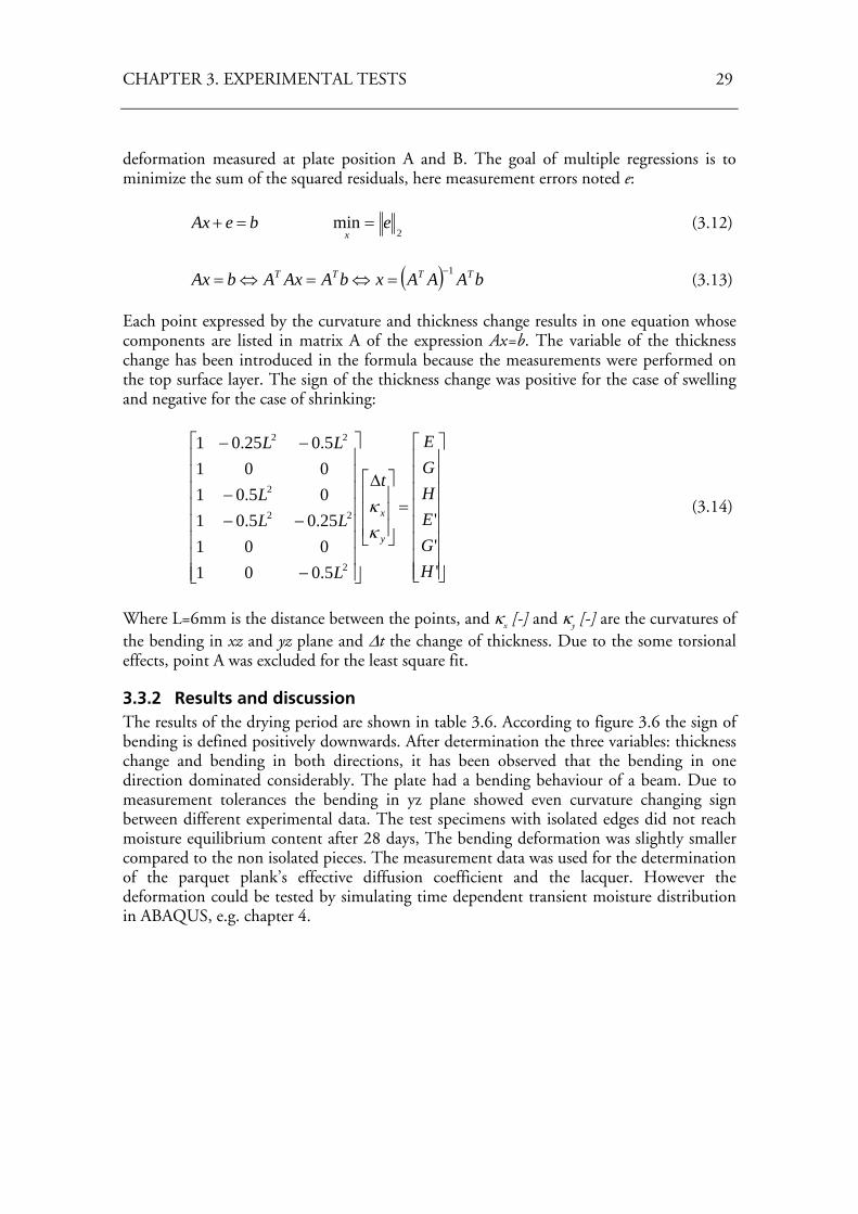
CHAPTER 3. EXPERIMENTAL TESTS 29
deformation measured at plate position A and B. The goal of multiple regressions is to minimize the sum of the squared residuals, here measurement errors noted e:
beAx =+ 2
min ex
= (3.12)
( ) bAAAxbAAxAbAx TTTT 1−=⇔=⇔= (3.13)
Each point expressed by the curvature and thickness change results in one equation whose components are listed in matrix A of the expression Ax=b. The variable of the thickness change has been introduced in the formula because the measurements were performed on the top surface layer. The sign of the thickness change was positive for the case of swelling and negative for the case of shrinking:
⎥⎥⎥⎥⎥⎥⎥⎥
⎦
⎤
⎢⎢⎢⎢⎢⎢⎢⎢
⎣
⎡
=⎥⎥⎥
⎦
⎤
⎢⎢⎢
⎣
⎡Δ
⎥⎥⎥⎥⎥⎥⎥⎥
⎦
⎤
⎢⎢⎢⎢⎢⎢⎢⎢
⎣
⎡
−
−−−
−−
'''
5.00100125.05.0105.010015.025.01
2
22
2
22
HGEHGE
t
L
LLL
LL
y
x
κκ (3.14)
Where L=6mm is the distance between the points, and κx [-] and κy [-] are the curvatures of the bending in xz and yz plane and Δt the change of thickness. Due to the some torsional effects, point A was excluded for the least square fit.
3.3.2 Results and discussion The results of the drying period are shown in table 3.6. According to figure 3.6 the sign of bending is defined positively downwards. After determination the three variables: thickness change and bending in both directions, it has been observed that the bending in one direction dominated considerably. The plate had a bending behaviour of a beam. Due to measurement tolerances the bending in yz plane showed even curvature changing sign between different experimental data. The test specimens with isolated edges did not reach moisture equilibrium content after 28 days, The bending deformation was slightly smaller compared to the non isolated pieces. The measurement data was used for the determination of the parquet plank’s effective diffusion coefficient and the lacquer. However the deformation could be tested by simulating time dependent transient moisture distribution in ABAQUS, e.g. chapter 4.
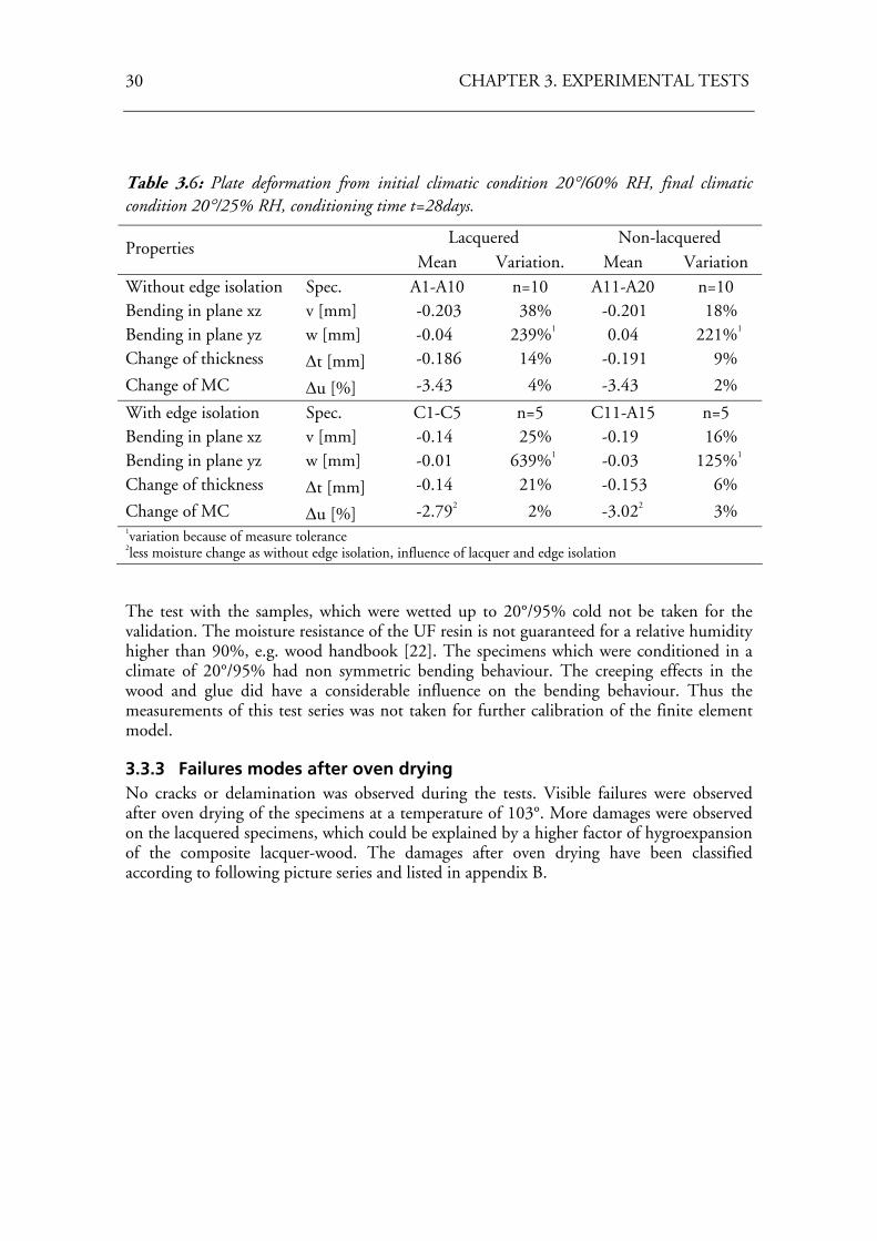
30 CHAPTER 3. EXPERIMENTAL TESTS
Table 3.6: Plate deformation from initial climatic condition 20°/60% RH, final climatic condition 20°/25% RH, conditioning time t=28days.
Lacquered Non-lacquered Properties
Mean Variation. Mean Variation Without edge isolation Spec. A1-A10 n=10 A11-A20 n=10 Bending in plane xz v [mm] -0.203 38% -0.201 18% Bending in plane yz w [mm] -0.04 239%1 0.04 221%1
Change of thickness Δt [mm] -0.186 14% -0.191 9%
Change of MC Δu [%] -3.43 4% -3.43 2%
With edge isolation Spec. C1-C5 n=5 C11-A15 n=5 Bending in plane xz v [mm] -0.14 25% -0.19 16% Bending in plane yz w [mm] -0.01 639%1 -0.03 125%1
Change of thickness Δt [mm] -0.14 21% -0.153 6%
Change of MC Δu [%] -2.792 2% -3.022 3% 1variation because of measure tolerance 2less moisture change as without edge isolation, influence of lacquer and edge isolation
The test with the samples, which were wetted up to 20°/95% cold not be taken for the validation. The moisture resistance of the UF resin is not guaranteed for a relative humidity higher than 90%, e.g. wood handbook [22]. The specimens which were conditioned in a climate of 20°/95% had non symmetric bending behaviour. The creeping effects in the wood and glue did have a considerable influence on the bending behaviour. Thus the measurements of this test series was not taken for further calibration of the finite element model.
3.3.3 Failures modes after oven drying No cracks or delamination was observed during the tests. Visible failures were observed after oven drying of the specimens at a temperature of 103°. More damages were observed on the lacquered specimens, which could be explained by a higher factor of hygroexpansion of the composite lacquer-wood. The damages after oven drying have been classified according to following picture series and listed in appendix B.
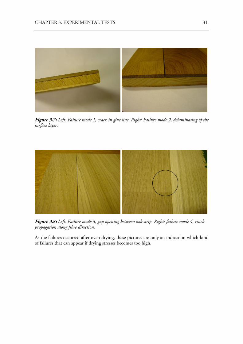
CHAPTER 3. EXPERIMENTAL TESTS 31
Figure 3.7: Left: Failure mode 1, crack in glue line. Right: Failure mode 2, delaminating of the surface layer.
Figure 3.8: Left: Failure mode 3, gap opening between oak strip. Right: failure mode 4, crack propagation along fibre direction.
As the failures occurred after oven drying, these pictures are only an indication which kind of failures that can appear if drying stresses becomes too high.

32 CHAPTER 3. EXPERIMENTAL TESTS
33
Chapter 4
Calibration and validation
4.1 Introduction Numerical methods such as the finite element method (FEM) are used for solving differential equations. The application of the finite element method can be used for the design of wood flooring products, for example. Computer data entry of physical and material specific properties needs to be done carefully. Therefore, each model and its behaviour under different load cases has to be tested for its validity. A good modelling of the reality demands knowledge about material properties, calculation methods and correct interpretation of the results. The literature available on parquet flooring systems is limited, because much of the research in this sector has been done in-house by industry. This means that much of the knowledge is held by these companies. Some tests have been performed in the context of this diploma thesis, see chapter 3, because of the absence of wood flooring specific data. This chapter treats the calibration and validation of finite element models based on the simulation of moisture transport and its induced deformations. The influence of the glue line (UF resin) and the lacquer to the moisture transport and the moisture induced deformations are studied closely in this chapter. The rheological behaviour of the composite resin – wood has an important influence on the stress distribution in wood composites products. The chapter is divided in two main sections, one regarding the modelling of the moisture transport and the second regarding the calibration and validation of the model and comparing it to test results, which were described in chapter 3.
4.2 Calibration of the moisture transport The finite element modelling of moisture transport in wood flooring systems was performed using the software ABAQUS [1]. The velocity of the moisture transport through the parquet planks depends on the induced boundary conditions, the diffusion coefficients of the different layers, the influence of the glue line and the treatment of the covering layer. For the calibration model, one dimensional moisture transport with moisture exchanging surface on the top and bottom surface was assumed. Thus results were compared to tests specimens with moisture isolated edges, e.g. chapter 3.
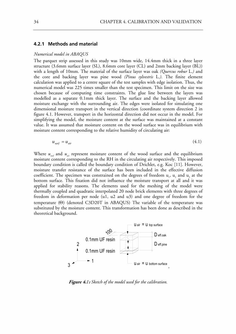
34 CHAPTER 4. CALIBRATION AND VALIDATION
4.2.1 Methods and material
Numerical model in ABAQUS The parquet strip assessed in this study was 10mm wide, 14.4mm thick in a three layer structure (3.6mm surface layer (SL), 8.6mm core layer (CL) and 2mm backing layer (BL)) with a length of 10mm. The material of the surface layer was oak (Quercus robur L.) and the core and backing layer was pine wood (Pinus sylvestris L.). The finite element calculation was applied to a centre square of the test samples with edge isolation. Thus, the numerical model was 225 times smaller than the test specimen. This limit on the size was chosen because of computing time constraints. The glue line between the layers was modelled as a separate 0.1mm thick layer. The surface and the backing layer allowed moisture exchange with the surrounding air. The edges were isolated for simulating one dimensional moisture transport in the vertical direction (coordinate system direction 2 in figure 4.1. However, transport in the horizontal direction did not occur in the model. For simplifying the model, the moisture content at the surface was maintained at a constant value. It was assumed that moisture content on the wood surface was in equilibrium with moisture content corresponding to the relative humidity of circulating air: airsurf uu = (4.1)
Where usurf and uair represent moisture content of the wood surface and the equilibrium moisture content corresponding to the RH in the circulating air respectively. This imposed boundary condition is called the boundary condition of Drichlet, e.g. Koc [11]. However, moisture transfer resistance of the surface has been included in the effective diffusion coefficient. The specimen was constrained on the degrees of freedom u1, u2 and u3 at the bottom surface. This fixation did not influence the moisture transport at all and it was applied for stability reasons. The elements used for the meshing of the model were thermally coupled and quadratic interpolated 20 node brick elements with three degrees of freedom in deformation per node (u1, u2 and u3) and one degree of freedom for the temperature (Θ) (denoted C3D20T in ABAQUS) The variable of the temperature was substituted by the moisture content. This transformation has been done as described in the theoretical background.
2
31
D
D
eff.oak
eff.pine
u air = u top surface
u air bottom surface= u
1000.1mm UF resin
0.1mm UF resin
,
Figure 4.1: Sketch of the model used for the calibration.
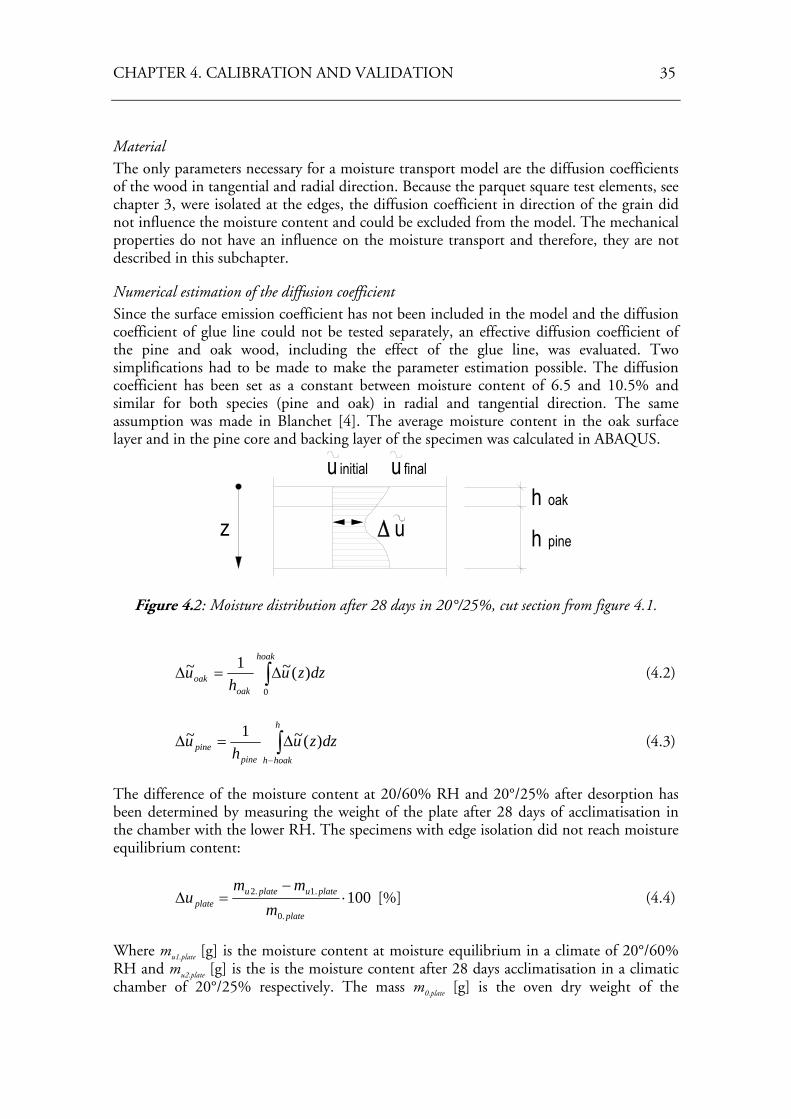
CHAPTER 4. CALIBRATION AND VALIDATION 35
Material The only parameters necessary for a moisture transport model are the diffusion coefficients of the wood in tangential and radial direction. Because the parquet square test elements, see chapter 3, were isolated at the edges, the diffusion coefficient in direction of the grain did not influence the moisture content and could be excluded from the model. The mechanical properties do not have an influence on the moisture transport and therefore, they are not described in this subchapter.
Numerical estimation of the diffusion coefficient Since the surface emission coefficient has not been included in the model and the diffusion coefficient of glue line could not be tested separately, an effective diffusion coefficient of the pine and oak wood, including the effect of the glue line, was evaluated. Two simplifications had to be made to make the parameter estimation possible. The diffusion coefficient has been set as a constant between moisture content of 6.5 and 10.5% and similar for both species (pine and oak) in radial and tangential direction. The same assumption was made in Blanchet [4]. The average moisture content in the oak surface layer and in the pine core and backing layer of the specimen was calculated in ABAQUS.
u initial u final
Δ uzh
h
oak
pine
Figure 4.2: Moisture distribution after 28 days in 20°/25%, cut section from figure 4.1.
∫ Δ=Δhoak
oakoak dzzu
hu
0
)(~1~ (4.2)
∫−
Δ=Δh
hoakhpinepine dzzu
hu )(~1~ (4.3)
The difference of the moisture content at 20/60% RH and 20°/25% after desorption has been determined by measuring the weight of the plate after 28 days of acclimatisation in the chamber with the lower RH. The specimens with edge isolation did not reach moisture equilibrium content:
100.0
.1.2 ⋅−
=Δplate
plateuplateuplate m
mmu [%] (4.4)
Where mu1.plate [g] is the moisture content at moisture equilibrium in a climate of 20°/60% RH and mu2.plate [g] is the is the moisture content after 28 days acclimatisation in a climatic chamber of 20°/25% respectively. The mass m0.plate [g] is the oven dry weight of the
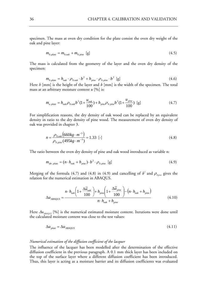
36 CHAPTER 4. CALIBRATION AND VALIDATION
specimen. The mass at oven dry condition for the plate consist the oven dry weight of the oak and pine layer: pineoakplate mmm .0.0.0 += [g] (4.5)
The mass is calculated from the geometry of the layer and the oven dry density of the specimen: 2
.02
.0.0 bhbhm pinepineoakoakplate ⋅⋅+⋅⋅= ρρ [g] (4.6)
Here h [mm] is the height of the layer and b [mm] is the width of the specimen. The total mass at an arbitrary moisture content u [%] is:
)100
1()100
1( 2.0
2.0.
pinepinepine
oakoakoakplateu
ubhubhm +++= ρρ [g] (4.7)
For simplification reasons, the dry density of oak wood can be replaced by an equivalent density in ratio to the dry density of pine wood. The measurement of oven dry density of oak was provided in chapter 3.
( )
33.1)495(
6603
.0
3.0 =
⋅⋅
= −
−
mkgmkg
npine
oak
ρρ
[-] (4.8)
The ratio between the oven dry density of pine and oak wood introduced as variable n: pinepineoakplatedtr bhhnm .0
2. )( ρ⋅⋅+⋅= [g] (4.9)
Merging of the formula (4.7) and (4.8) in (4.9) and cancelling of b2 and ρ0.pine gives the relation for the numerical estimation in ABAQUS.
( )
pineoak
pineoakpine
pineoak
oak
ABAQUS hhn
hhnu
huhnu
+⋅
+⋅−⎟⎟⎠
⎞⎜⎜⎝
⎛ Δ++⎟
⎠⎞
⎜⎝⎛ Δ
+⋅=Δ
100
~1
100
~1
(4.10)
Here ΔuABAQUS [%] is the numerical estimated moisture content. Iterations were done until the calculated moisture content was close to the test values: ABAQUSplate uu Δ=Δ (4.11)
Numerical estimation of the diffusion coefficient of the lacquer The influence of the lacquer has been modelled after the determination of the effective diffusion coefficient in the previous paragraph. A 0.1 mm thick layer has been included on the top of the surface layer where a different diffusion coefficient has been introduced. Thus, this layer is acting as a moisture barrier and its diffusion coefficients was evaluated
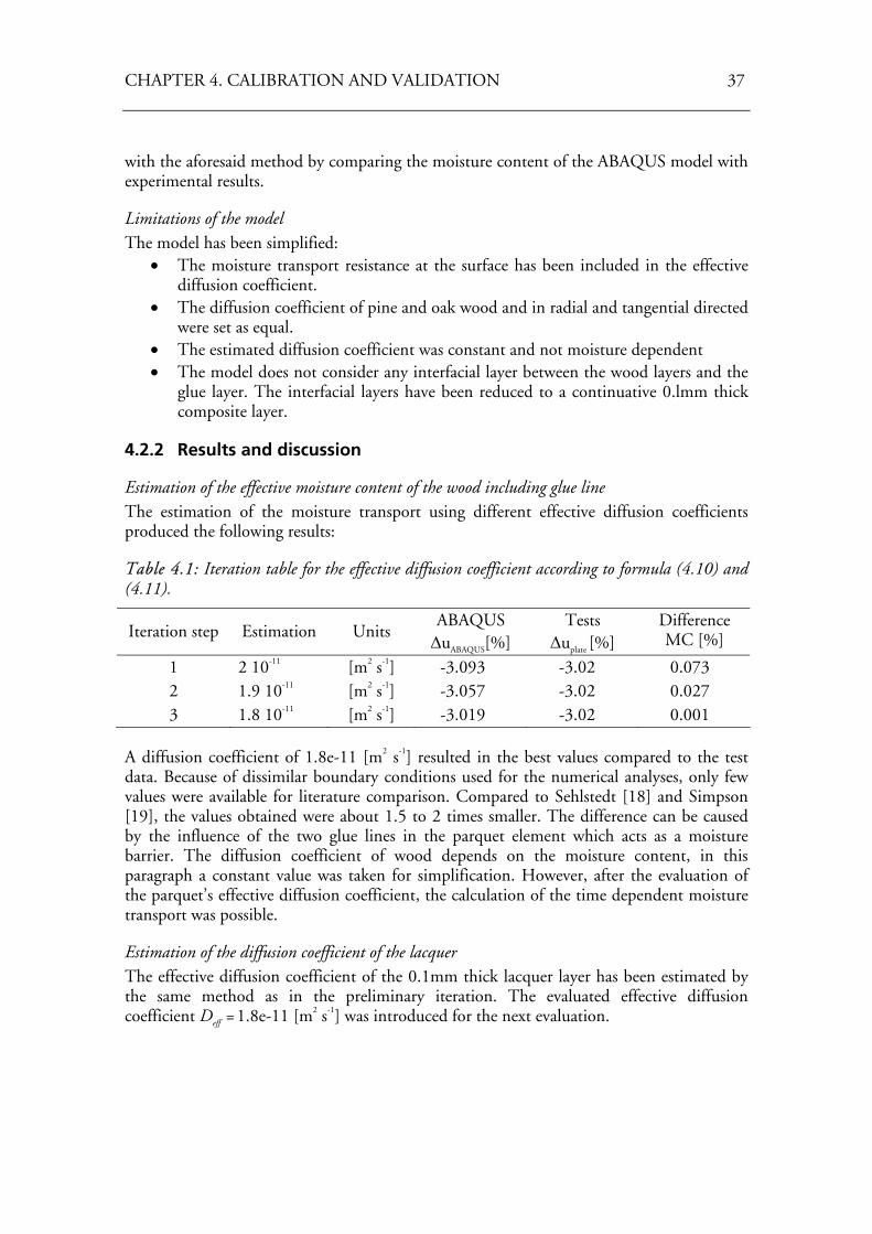
CHAPTER 4. CALIBRATION AND VALIDATION 37
with the aforesaid method by comparing the moisture content of the ABAQUS model with experimental results.
Limitations of the model The model has been simplified:
• The moisture transport resistance at the surface has been included in the effective diffusion coefficient.
• The diffusion coefficient of pine and oak wood and in radial and tangential directed were set as equal.
• The estimated diffusion coefficient was constant and not moisture dependent • The model does not consider any interfacial layer between the wood layers and the
glue layer. The interfacial layers have been reduced to a continuative 0.lmm thick composite layer.
4.2.2 Results and discussion
Estimation of the effective moisture content of the wood including glue line The estimation of the moisture transport using different effective diffusion coefficients produced the following results:
Table 4.1: Iteration table for the effective diffusion coefficient according to formula (4.10) and (4.11).
Iteration step Estimation Units ABAQUS
ΔuABAQUS[%] Tests
Δuplate [%] Difference MC [%]
1 2 10-11 [m2 s-1] -3.093 -3.02 0.073 2 1.9 10-11 [m2 s-1] -3.057 -3.02 0.027 3 1.8 10-11 [m2 s-1] -3.019 -3.02 0.001
A diffusion coefficient of 1.8e-11 [m2 s-1] resulted in the best values compared to the test data. Because of dissimilar boundary conditions used for the numerical analyses, only few values were available for literature comparison. Compared to Sehlstedt [18] and Simpson [19], the values obtained were about 1.5 to 2 times smaller. The difference can be caused by the influence of the two glue lines in the parquet element which acts as a moisture barrier. The diffusion coefficient of wood depends on the moisture content, in this paragraph a constant value was taken for simplification. However, after the evaluation of the parquet’s effective diffusion coefficient, the calculation of the time dependent moisture transport was possible.
Estimation of the diffusion coefficient of the lacquer The effective diffusion coefficient of the 0.1mm thick lacquer layer has been estimated by the same method as in the preliminary iteration. The evaluated effective diffusion coefficient Deff = 1.8e-11 [m2 s-1] was introduced for the next evaluation.
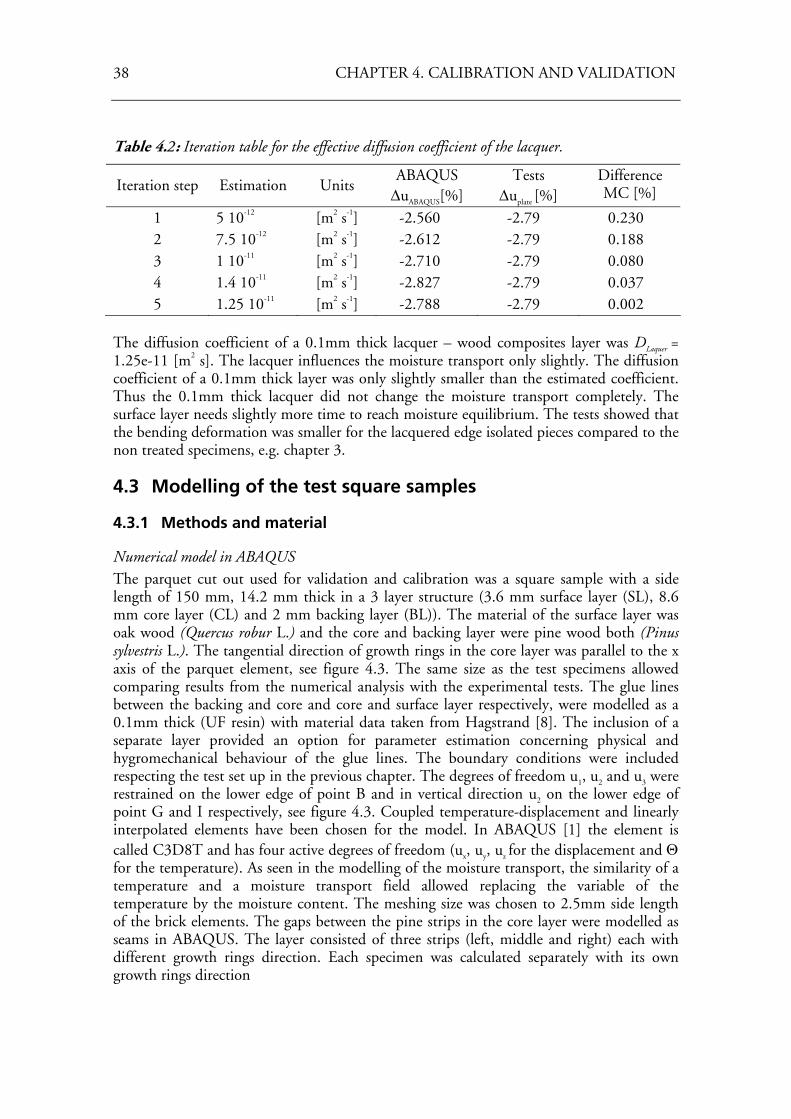
38 CHAPTER 4. CALIBRATION AND VALIDATION
Table 4.2: Iteration table for the effective diffusion coefficient of the lacquer.
Iteration step Estimation Units ABAQUS
ΔuABAQUS[%] Tests
Δuplate [%] Difference MC [%]
1 5 10-12 [m2 s-1] -2.560 -2.79 0.230 2 7.5 10-12 [m2 s-1] -2.612 -2.79 0.188 3 1 10-11 [m2 s-1] -2.710 -2.79 0.080 4 1.4 10-11 [m2 s-1] -2.827 -2.79 0.037 5 1.25 10-11 [m2 s-1] -2.788 -2.79 0.002
The diffusion coefficient of a 0.1mm thick lacquer – wood composites layer was DLaquer = 1.25e-11 [m2 s]. The lacquer influences the moisture transport only slightly. The diffusion coefficient of a 0.1mm thick layer was only slightly smaller than the estimated coefficient. Thus the 0.1mm thick lacquer did not change the moisture transport completely. The surface layer needs slightly more time to reach moisture equilibrium. The tests showed that the bending deformation was smaller for the lacquered edge isolated pieces compared to the non treated specimens, e.g. chapter 3.
4.3 Modelling of the test square samples
4.3.1 Methods and material
Numerical model in ABAQUS The parquet cut out used for validation and calibration was a square sample with a side length of 150 mm, 14.2 mm thick in a 3 layer structure (3.6 mm surface layer (SL), 8.6 mm core layer (CL) and 2 mm backing layer (BL)). The material of the surface layer was oak wood (Quercus robur L.) and the core and backing layer were pine wood both (Pinus sylvestris L.). The tangential direction of growth rings in the core layer was parallel to the x axis of the parquet element, see figure 4.3. The same size as the test specimens allowed comparing results from the numerical analysis with the experimental tests. The glue lines between the backing and core and core and surface layer respectively, were modelled as a 0.1mm thick (UF resin) with material data taken from Hagstrand [8]. The inclusion of a separate layer provided an option for parameter estimation concerning physical and hygromechanical behaviour of the glue lines. The boundary conditions were included respecting the test set up in the previous chapter. The degrees of freedom u1, u2 and u3 were restrained on the lower edge of point B and in vertical direction u2 on the lower edge of point G and I respectively, see figure 4.3. Coupled temperature-displacement and linearly interpolated elements have been chosen for the model. In ABAQUS [1] the element is called C3D8T and has four active degrees of freedom (ux, uy, uz for the displacement and Θ for the temperature). As seen in the modelling of the moisture transport, the similarity of a temperature and a moisture transport field allowed replacing the variable of the temperature by the moisture content. The meshing size was chosen to 2.5mm side length of the brick elements. The gaps between the pine strips in the core layer were modelled as seams in ABAQUS. The layer consisted of three strips (left, middle and right) each with different growth rings direction. Each specimen was calculated separately with its own growth rings direction
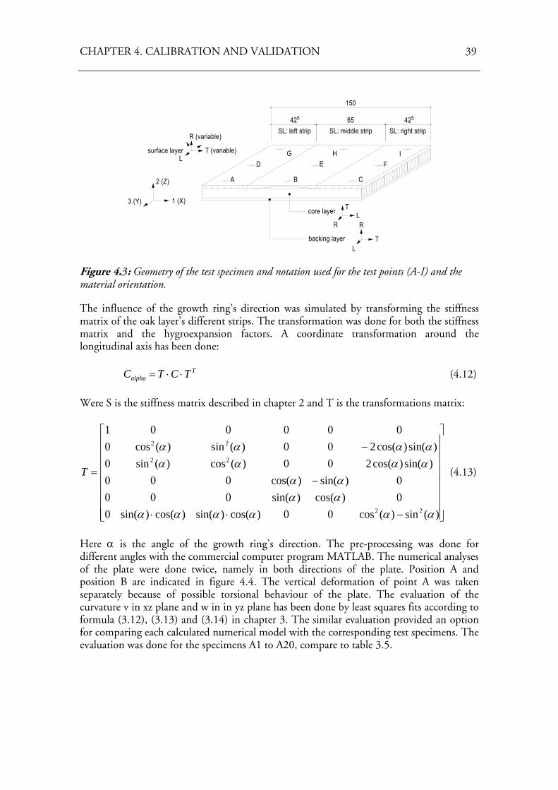
CHAPTER 4. CALIBRATION AND VALIDATION 39
3 (Y) 1 (X)
2 (Z) A B C
D E FHG IT (variable)
R (variable)
surface layer
core layer TL
backing layer
R
T
L
425 65 425
150
R
L
SL: left strip SL: middle strip SL: right strip
Figure 4.3: Geometry of the test specimen and notation used for the test points (A-I) and the material orientation.
The influence of the growth ring’s direction was simulated by transforming the stiffness matrix of the oak layer’s different strips. The transformation was done for both the stiffness matrix and the hygroexpansion factors. A coordinate transformation around the longitudinal axis has been done: T
alpha TCTC ⋅⋅= (4.12)
Were S is the stiffness matrix described in chapter 2 and T is the transformations matrix:
⎥⎥⎥⎥⎥⎥⎥⎥
⎦
⎤
⎢⎢⎢⎢⎢⎢⎢⎢
⎣
⎡
−⋅⋅
−
−
=
)(sin)(cos00)cos()sin()cos()sin(00)cos()sin(0000)sin()cos(000
)sin()cos(200)(cos)(sin0)sin()cos(200)(sin)(cos0
000001
22
22
22
αααααααααα
αααααααα
T (4.13)
Here α is the angle of the growth ring’s direction. The pre-processing was done for different angles with the commercial computer program MATLAB. The numerical analyses of the plate were done twice, namely in both directions of the plate. Position A and position B are indicated in figure 4.4. The vertical deformation of point A was taken separately because of possible torsional behaviour of the plate. The evaluation of the curvature v in xz plane and w in in yz plane has been done by least squares fits according to formula (3.12), (3.13) and (3.14) in chapter 3. The similar evaluation provided an option for comparing each calculated numerical model with the corresponding test specimens. The evaluation was done for the specimens A1 to A20, compare to table 3.5.
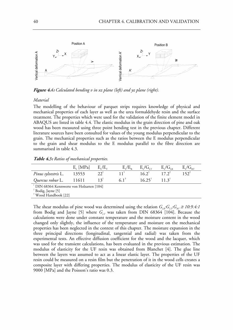
40 CHAPTER 4. CALIBRATION AND VALIDATION
YX
Z
Verti
cal d
efor
mat
ion A
v
A
Position A
XY
Z
A'
Position B
Verri
cal d
efor
mat
ion A
'
w
Figure 4.4: Calculated bending v in xz plane (left) and yz plane (right).
Material The modelling of the behaviour of parquet strips requires knowledge of physical and mechanical properties of each layer as well as the urea formaldehyde resin and the surface treatment. The properties which were used for the validation of the finite element model in ABAQUS are listed in table 4.4. The elastic modulus in the grain direction of pine and oak wood has been measured using three point bending test in the previous chapter. Different literature sources have been consulted for values of the young modulus perpendicular to the grain. The mechanical properties such as the ratios between the E modulus perpendicular to the grain and shear modulus to the E modulus parallel to the fibre direction are summarised in table 4.3.
Table 4.3: Ratios of mechanical properties.
EL [MPa] EL/ET EL/ER EL/GLT EL/GLR EL/GRT
Pinus sylvestris L. 13553 221 111 16.21 17.22 1522
Quercus robur L. 11611 131 6.13 16.251 11.31 1 DIN 68364 Kennwerte von Holzarten [104] 2 Bodig, Jayne [5] 3 Wood Handbook [22] The shear modulus of pine wood was determined using the relation GLR:GLT:GRT ≅ 10:9.4:1 from Bodig and Jayne [5] where GLT was taken from DIN 68364 [104]. Because the calculations were done under constant temperature and the moisture content in the wood changed only slightly, the influence of the temperature and moisture on the mechanical properties has been neglected in the context of this chapter. The moisture expansion in the three principal directions (longitudinal, tangential and radial) was taken from the experimental tests. An effective diffusion coefficient for the wood and the lacquer, which was used for the transient calculations, has been evaluated in the previous estimation. The modulus of elasticity for the UF resin was obtained from Blanchet [4]. The glue line between the layers was assumed to act as a linear elastic layer. The properties of the UF resin could be measured on a resin film but the penetration of it in the wood cells creates a composite layer with differing properties. The modulus of elasticity of the UF resin was 9000 [MPa] and the Poisson’s ratio was 0.3.
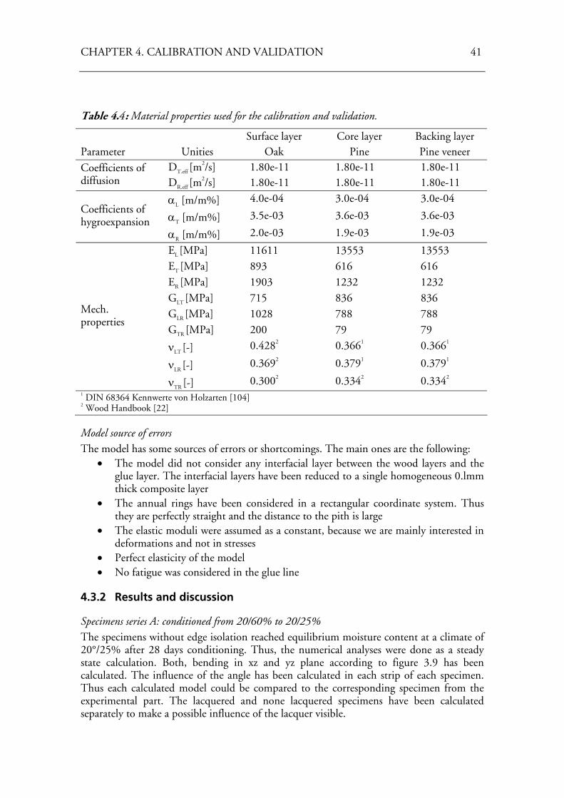
CHAPTER 4. CALIBRATION AND VALIDATION 41
Table 4.4: Material properties used for the calibration and validation.
Surface layer Core layer Backing layer Parameter Unities Oak Pine Pine veneer
DT.eff [m2/s] 1.80e-11 1.80e-11 1.80e-11 Coefficients of
diffusion DR.eff [m2/s] 1.80e-11 1.80e-11 1.80e-11
αL [m/m%] 4.0e-04 3.0e-04 3.0e-04
αT [m/m%] 3.5e-03 3.6e-03 3.6e-03 Coefficients of hygroexpansion
αR [m/m%] 2.0e-03 1.9e-03 1.9e-03
EL [MPa] 11611 13553 13553 ET [MPa] 893 616 616 ER [MPa] 1903 1232 1232 GLT [MPa] 715 836 836 GLR [MPa] 1028 788 788 GTR [MPa] 200 79 79
νLT [-] 0.4282 0.3661 0.3661
νLR [-] 0.3692 0.3791 0.3791
Mech. properties
νTR [-] 0.3002 0.3342 0.3342 1 DIN 68364 Kennwerte von Holzarten [104] 2 Wood Handbook [22]
Model source of errors The model has some sources of errors or shortcomings. The main ones are the following:
• The model did not consider any interfacial layer between the wood layers and the glue layer. The interfacial layers have been reduced to a single homogeneous 0.lmm thick composite layer
• The annual rings have been considered in a rectangular coordinate system. Thus they are perfectly straight and the distance to the pith is large
• The elastic moduli were assumed as a constant, because we are mainly interested in deformations and not in stresses
• Perfect elasticity of the model • No fatigue was considered in the glue line
4.3.2 Results and discussion
Specimens series A: conditioned from 20/60% to 20/25% The specimens without edge isolation reached equilibrium moisture content at a climate of 20°/25% after 28 days conditioning. Thus, the numerical analyses were done as a steady state calculation. Both, bending in xz and yz plane according to figure 3.9 has been calculated. The influence of the angle has been calculated in each strip of each specimen. Thus each calculated model could be compared to the corresponding specimen from the experimental part. The lacquered and none lacquered specimens have been calculated separately to make a possible influence of the lacquer visible.
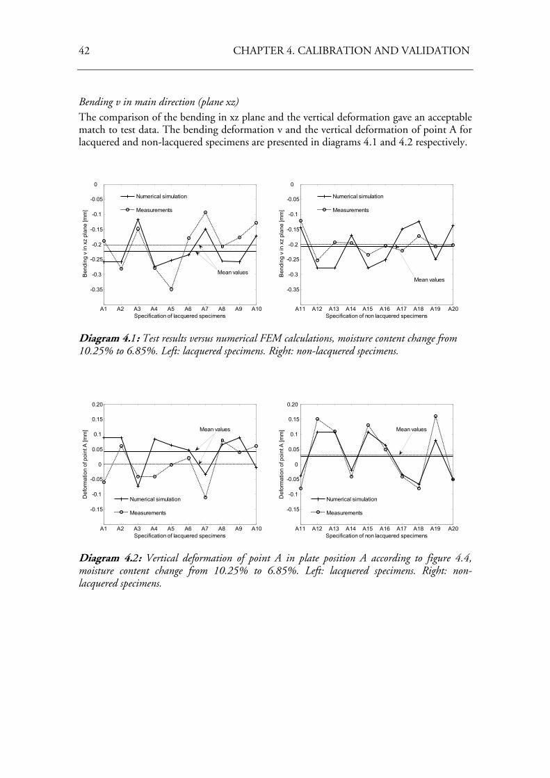
42 CHAPTER 4. CALIBRATION AND VALIDATION
Bending v in main direction (plane xz) The comparison of the bending in xz plane and the vertical deformation gave an acceptable match to test data. The bending deformation v and the vertical deformation of point A for lacquered and non-lacquered specimens are presented in diagrams 4.1 and 4.2 respectively.
A1 A2 A3 A4 A5 A6 A7 A8 A9 A10
-0.35
-0.3
-0.25
-0.2
-0.15
-0.1
-0.05
0
Specification of lacquered specimens
Ben
ding
v in
xz
plan
e [m
m]
Numerical simulation
Measurements
Mean values
A11 A12 A13 A14 A15 A16 A17 A18 A19 A20
-0.35
-0.3
-0.25
-0.2
-0.15
-0.1
-0.05
0
Specification of non lacquered specimens
Ben
ding
v in
xz
plan
e [m
m]
Numerical simulation
Measurements
Mean values
Diagram 4.1: Test results versus numerical FEM calculations, moisture content change from 10.25% to 6.85%. Left: lacquered specimens. Right: non-lacquered specimens.
A1 A2 A3 A4 A5 A6 A7 A8 A9 A10
-0.15
-0.1
-0.05
0
0.05
0.1
0.15
0.20
Specification of lacquered specimens
Def
orm
atio
n of
poi
nt A
[mm
]
Numerical simulation
Measurements
Mean values
A11 A12 A13 A14 A15 A16 A17 A18 A19 A20
-0.15
-0.1
-0.05
0
0.05
0.1
0.15
0.20
Specification of non lacquered specimens
Def
orm
atio
n of
poi
nt A
[mm
]
Numerical simulation
Measurements
Mean values
Diagram 4.2: Vertical deformation of point A in plate position A according to figure 4.4, moisture content change from 10.25% to 6.85%. Left: lacquered specimens. Right: non-lacquered specimens.
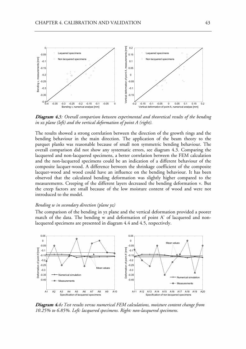
CHAPTER 4. CALIBRATION AND VALIDATION 43
-0.4 -0.35 -0.3 -0.25 -0.2 -0.15 -0.1 -0.05 0-0.4
-0.35
-0.3
-0.25
-0.2
-0.15
-0.1
-0.05
0
Bending v, numerical analyse [mm]
Ben
ding
v, m
easu
rem
ents
[mm
]
Laquered specimens
Non lacquered specimens
-0.2 -0.15 -0.1 -0.05 0 0.05 0.1 0.15 0.2
-0.15
-0.1
-0.05
0
0.05
0.1
0.15
0.2
Vertical deformation of point A, numerical analyse [mm]
Ver
tical
def
orm
atio
n of
poi
nt A
, mea
sure
men
ts [m
m]
Laquered specimens
Non lacquered specimens
Diagram 4.3: Overall comparison between experimental and theoretical results of the bending in xz plane (left) and the vertical deformation of point A (right).
The results showed a strong correlation between the direction of the growth rings and the bending behaviour in the main direction. The application of the beam theory to the parquet planks was reasonable because of small non symmetric bending behaviour. The overall comparison did not show any systematic errors, see diagram 4.3. Comparing the lacquered and non-lacquered specimens, a better correlation between the FEM calculation and the non-lacquered specimens could be an indication of a different behaviour of the composite lacquer-wood. A difference between the shrinkage coefficient of the composite lacquer-wood and wood could have an influence on the bending behaviour. It has been observed that the calculated bending deformation was slightly higher compared to the measurements. Creeping of the different layers decreased the bending deformation v. But the creep factors are small because of the low moisture content of wood and were not introduced to the model.
Bending w in secondary direction (plane yz) The comparison of the bending in yz plane and the vertical deformation provided a poorer match of the data. The bending w and deformation of point A’ of lacquered and non-lacquered specimens are presented in diagram 4.4 and 4.5, respectively.
A1 A2 A3 A4 A5 A6 A7 A8 A9 A10
-0.40
-0.35
-0.3
-0.25
-0.2
-0.15
-0.1
-0.05
0
0.05
Specification of lacquered specimens
Def
orm
atio
n of
poi
nt A
'[mm
]
Numerical simulation
Measurements
Mean values
A11 A12 A13 A14 A15 A16 A17 A18 A19 A20
-0.40
-0.35
-0.3
-0.25
-0.2
-0.15
-0.1
-0.05
0
0.05
Specification of non lacquered specimens
Def
orm
atio
n of
poi
nt A
' [m
m]
Numerical simulation
Measurements
Mean values
Diagram 4.4: Test results versus numerical FEM calculations, moisture content change from 10.25% to 6.85%. Left: lacquered specimens. Right: non-lacquered specimens.
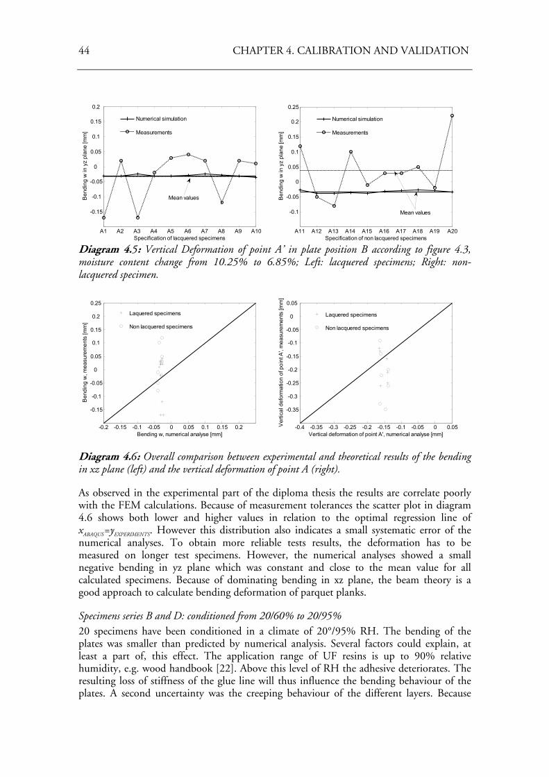
44 CHAPTER 4. CALIBRATION AND VALIDATION
A1 A2 A3 A4 A5 A6 A7 A8 A9 A10
-0.15
-0.1
-0.05
0
0.05
0.1
0.15
0.2
Specification of lacquered specimens
Ben
ding
w in
yz
plan
e [m
m]
Numerical simulation
Measurements
Mean values
A11 A12 A13 A14 A15 A16 A17 A18 A19 A20
-0.1
-0.05
0
0.05
0.1
0.15
0.2
0.25
Specification of non lacquered specimens
Ben
ding
w in
yz
plan
e [m
m]
Numerical simulation
Measurements
Mean values
Diagram 4.5: Vertical Deformation of point A’ in plate position B according to figure 4.3, moisture content change from 10.25% to 6.85%; Left: lacquered specimens; Right: non-lacquered specimen.
-0.2 -0.15 -0.1 -0.05 0 0.05 0.1 0.15 0.2
-0.15
-0.1
-0.05
0
0.05
0.1
0.15
0.2
0.25
Bending w, numerical analyse [mm]
Ben
ding
w, m
easu
rem
ents
[mm
]
Laquered specimens
Non lacquered specimens
-0.4 -0.35 -0.3 -0.25 -0.2 -0.15 -0.1 -0.05 0 0.05
-0.35
-0.3
-0.25
-0.2
-0.15
-0.1
-0.05
0
0.05
Vertical deformation of point A', numerical analyse [mm]
Ver
tical
def
orm
atio
n of
poi
nt A
', m
easu
rem
ents
[mm
]
Laquered specimens
Non lacquered specimens
Diagram 4.6: Overall comparison between experimental and theoretical results of the bending in xz plane (left) and the vertical deformation of point A (right).
As observed in the experimental part of the diploma thesis the results are correlate poorly with the FEM calculations. Because of measurement tolerances the scatter plot in diagram 4.6 shows both lower and higher values in relation to the optimal regression line of xABAQUS=yEXPERIMENTS. However this distribution also indicates a small systematic error of the numerical analyses. To obtain more reliable tests results, the deformation has to be measured on longer test specimens. However, the numerical analyses showed a small negative bending in yz plane which was constant and close to the mean value for all calculated specimens. Because of dominating bending in xz plane, the beam theory is a good approach to calculate bending deformation of parquet planks.
Specimens series B and D: conditioned from 20/60% to 20/95% 20 specimens have been conditioned in a climate of 20°/95% RH. The bending of the plates was smaller than predicted by numerical analysis. Several factors could explain, at least a part of, this effect. The application range of UF resins is up to 90% relative humidity, e.g. wood handbook [22]. Above this level of RH the adhesive deteriorates. The resulting loss of stiffness of the glue line will thus influence the bending behaviour of the plates. A second uncertainty was the creeping behaviour of the different layers. Because
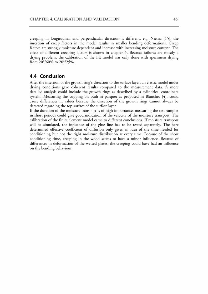
CHAPTER 4. CALIBRATION AND VALIDATION 45
creeping in longitudinal and perpendicular direction is different, e.g. Niemz [15], the insertion of creep factors in the model results in smaller bending deformations. Creep factors are strongly moisture dependent and increase with increasing moisture content. The effect of different creeping factors is shown in chapter 5. Because failures are mostly a drying problem, the calibration of the FE model was only done with specimens drying from 20°/60% to 20°/25%.
4.4 Conclusion After the insertion of the growth ring’s direction to the surface layer, an elastic model under drying conditions gave coherent results compared to the measurement data. A more detailed analysis could include the growth rings as described by a cylindrical coordinate system. Measuring the cupping on built-in parquet as proposed in Blanchet [4], could cause differences in values because the direction of the growth rings cannot always be detected regarding the top surface of the surface layer. If the duration of the moisture transport is of high importance, measuring the test samples in short periods could give good indication of the velocity of the moisture transport. The calibration of the finite element model came to different conclusions. If moisture transport will be simulated, the influence of the glue line has to be tested separately. The here determined effective coefficient of diffusion only gives an idea of the time needed for conditioning but not the right moisture distribution at every time. Because of the short conditioning time, creeping in the wood seems to have a minor influence. Because of differences in deformation of the wetted plates, the creeping could have had an influence on the bending behaviour.

46 CHAPTER 4. CALIBRATION AND VALIDATION
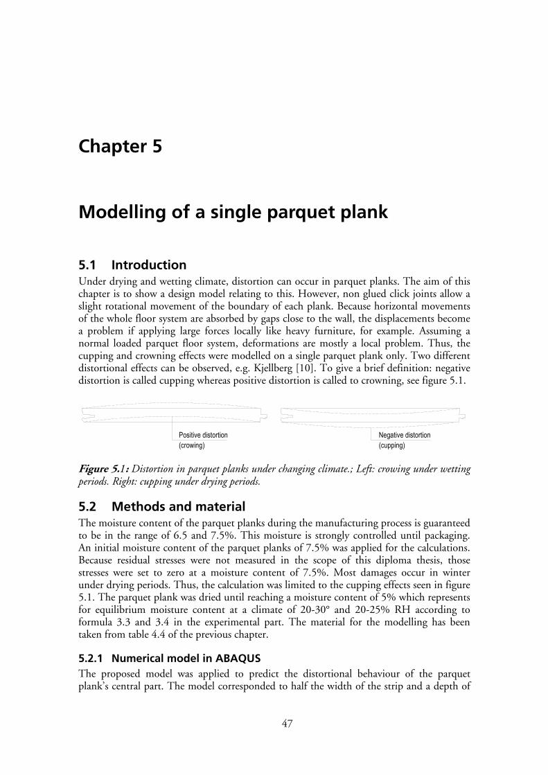
47
Chapter 5
Modelling of a single parquet plank
5.1 Introduction Under drying and wetting climate, distortion can occur in parquet planks. The aim of this chapter is to show a design model relating to this. However, non glued click joints allow a slight rotational movement of the boundary of each plank. Because horizontal movements of the whole floor system are absorbed by gaps close to the wall, the displacements become a problem if applying large forces locally like heavy furniture, for example. Assuming a normal loaded parquet floor system, deformations are mostly a local problem. Thus, the cupping and crowning effects were modelled on a single parquet plank only. Two different distortional effects can be observed, e.g. Kjellberg [10]. To give a brief definition: negative distortion is called cupping whereas positive distortion is called to crowning, see figure 5.1.
Positive distortion(crowing)
Negative distortion(cupping)
Figure 5.1: Distortion in parquet planks under changing climate.; Left: crowing under wetting periods. Right: cupping under drying periods.
5.2 Methods and material The moisture content of the parquet planks during the manufacturing process is guaranteed to be in the range of 6.5 and 7.5%. This moisture is strongly controlled until packaging. An initial moisture content of the parquet planks of 7.5% was applied for the calculations. Because residual stresses were not measured in the scope of this diploma thesis, those stresses were set to zero at a moisture content of 7.5%. Most damages occur in winter under drying periods. Thus, the calculation was limited to the cupping effects seen in figure 5.1. The parquet plank was dried until reaching a moisture content of 5% which represents for equilibrium moisture content at a climate of 20-30° and 20-25% RH according to formula 3.3 and 3.4 in the experimental part. The material for the modelling has been taken from table 4.4 of the previous chapter.
5.2.1 Numerical model in ABAQUS The proposed model was applied to predict the distortional behaviour of the parquet plank’s central part. The model corresponded to half the width of the strip and a depth of
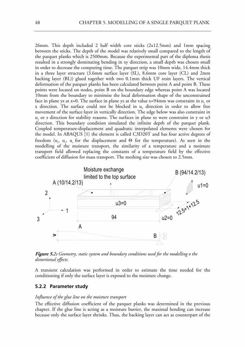
48 CHAPTER 5. MODELLING OF A SINGLE PARQUET PLANK
26mm. This depth included 2 half width core sticks (2x12.5mm) and 1mm spacing between the sticks. The depth of the model was relatively small compared to the length of the parquet planks which is 2500mm. Because the experimental part of the diploma thesis resulted in a strongly dominating bending in xy direction, a small depth was chosen small in order to decrease the computing time. The parquet strip was 10mm wide, 14.4mm thick in a three layer structure (3.6mm surface layer (SL), 8.6mm core layer (CL) and 2mm backing layer (BL)) glued together with two 0.1mm thick UF resin layers. The vertical deformation of the parquet planks has been calculated between point A and point B. These points were located on nodes, point B on the boundary edge whereas point A was located 10mm from the boundary to minimise the local deformation shape of the unconstrained face in plane yz at x=0. The surface in plane yz at the value x=94mm was constraint in u1 or x direction. The surface could not be blocked in u2 direction in order to allow free movement of the surface layer in vertically direction. The edge below was also constraint in u2 or z direction for stability reasons. The surfaces in plane xz were constraint in y or u3 direction. This boundary condition simulated the infinite depth of the parquet plank. Coupled temperature-displacement and quadratic interpolated elements were chosen for the model. In ABAQUS [1] the element is called C3D20T and has four active degrees of freedom (ux, uy, uz for the displacement and Θ for the temperature). As seen in the modelling of the moisture transport, the similarity of a temperature and a moisture transport field allowed replacing the constants of a temperature field by the effective coefficient of diffusion for mass transport. The meshing size was chosen to 2.5mm.
2
3 1 12.5+1+12.5
u2=0
u1=0A (10/14.2/13)
B (94/14.2/13)
u3=0
v BA
Moisture exchangelimited to the top surface
94
Figure 5.2: Geometry, static system and boundary conditions used for the modelling o the distortional effects.
A transient calculation was performed in order to estimate the time needed for the conditioning if only the surface layer is exposed to the moisture change.
5.2.2 Parameter study
Influence of the glue line on the moisture transport The effective diffusion coefficient of the parquet planks was determined in the previous chapter. If the glue line is acting as a moisture barrier, the maximal bending can increase because only the surface layer shrinks. Thus, the backing layer can act as counterpart of the
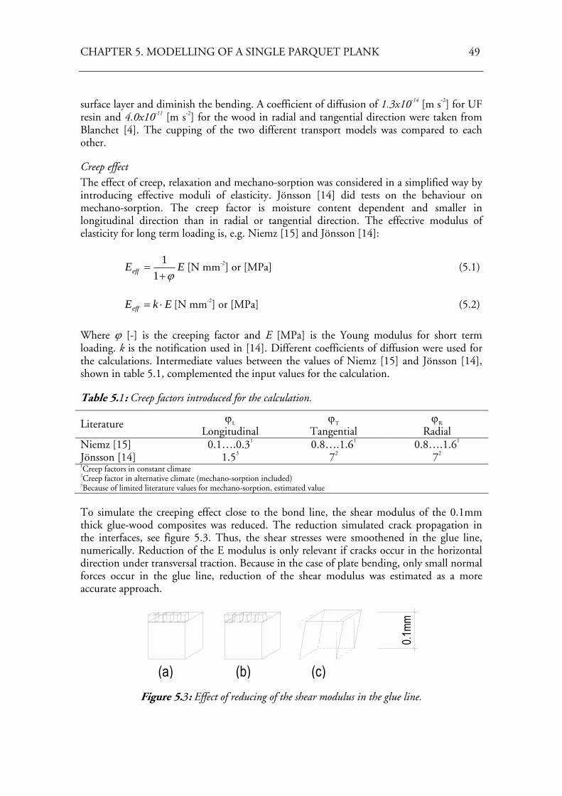
CHAPTER 5. MODELLING OF A SINGLE PARQUET PLANK 49
surface layer and diminish the bending. A coefficient of diffusion of 1.3x10⁻¹⁴ [m s-2] for UF resin and 4.0x10⁻¹¹ [m s-2] for the wood in radial and tangential direction were taken from Blanchet [4]. The cupping of the two different transport models was compared to each other.
Creep effect The effect of creep, relaxation and mechano-sorption was considered in a simplified way by introducing effective moduli of elasticity. Jönsson [14] did tests on the behaviour on mechano-sorption. The creep factor is moisture content dependent and smaller in longitudinal direction than in radial or tangential direction. The effective modulus of elasticity for long term loading is, e.g. Niemz [15] and Jönsson [14]:
EEeff ϕ+=
11
[N mm-2] or [MPa] (5.1)
EkEeff ⋅= [N mm-2] or [MPa] (5.2)
Where ϕ [-] is the creeping factor and E [MPa] is the Young modulus for short term loading. k is the notification used in [14]. Different coefficients of diffusion were used for the calculations. Intermediate values between the values of Niemz [15] and Jönsson [14], shown in table 5.1, complemented the input values for the calculation.
Table 5.1: Creep factors introduced for the calculation.
Literature ϕL
Longitudinal ϕT
Tangential ϕR
Radial Niemz [15] 0.1….0.31 0.8….1.61 0.8….1.61
Jönsson [14] 1.53 72 72
1Creep factors in constant climate 2Creep factor in alternative climate (mechano-sorption included) 3Because of limited literature values for mechano-sorption, estimated value
To simulate the creeping effect close to the bond line, the shear modulus of the 0.1mm thick glue-wood composites was reduced. The reduction simulated crack propagation in the interfaces, see figure 5.3. Thus, the shear stresses were smoothened in the glue line, numerically. Reduction of the E modulus is only relevant if cracks occur in the horizontal direction under transversal traction. Because in the case of plate bending, only small normal forces occur in the glue line, reduction of the shear modulus was estimated as a more accurate approach.
0.1m
m
(a) (b) (c)
Figure 5.3: Effect of reducing of the shear modulus in the glue line.
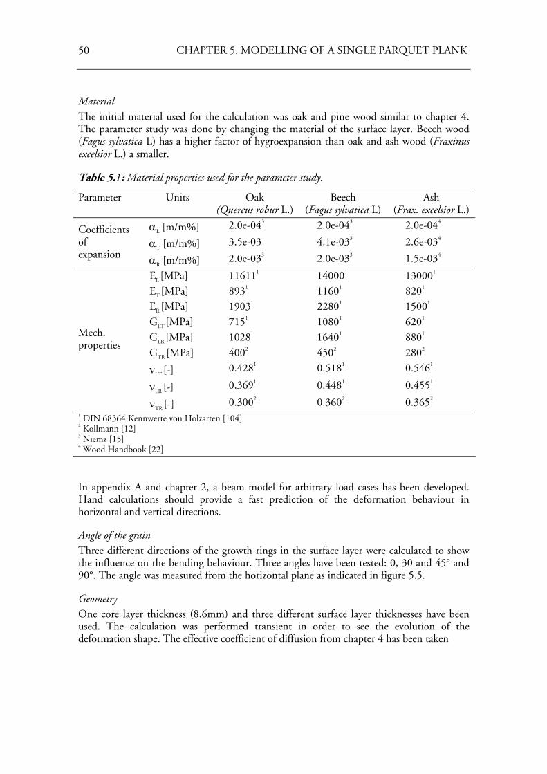
50 CHAPTER 5. MODELLING OF A SINGLE PARQUET PLANK
Material The initial material used for the calculation was oak and pine wood similar to chapter 4. The parameter study was done by changing the material of the surface layer. Beech wood (Fagus sylvatica L) has a higher factor of hygroexpansion than oak and ash wood (Fraxinus excelsior L.) a smaller.
Table 5.1: Material properties used for the parameter study.
Parameter Units Oak (Quercus robur L.)
Beech (Fagus sylvatica L)
Ash (Frax. excelsior L.)
αL [m/m%] 2.0e-043 2.0e-043 2.0e-044
αT [m/m%] 3.5e-03 4.1e-033 2.6e-034 Coefficients of expansion αR [m/m%] 2.0e-033 2.0e-033 1.5e-034
EL [MPa] 116111 140001 130001
ET [MPa] 8931 11601 8201
ER [MPa] 19031 22801 15001
GLT [MPa] 7151 10801 6201
GLR [MPa] 10281 16401 8801
GTR [MPa] 4002 4502 2802
νLT [-] 0.4281 0.5181 0.5461
νLR [-] 0.3691 0.4481 0.4551
Mech. properties
νTR [-] 0.3002 0.3602 0.3652 1 DIN 68364 Kennwerte von Holzarten [104] 2 Kollmann [12] 3 Niemz [15] 4 Wood Handbook [22]
In appendix A and chapter 2, a beam model for arbitrary load cases has been developed. Hand calculations should provide a fast prediction of the deformation behaviour in horizontal and vertical directions.
Angle of the grain Three different directions of the growth rings in the surface layer were calculated to show the influence on the bending behaviour. Three angles have been tested: 0, 30 and 45° and 90°. The angle was measured from the horizontal plane as indicated in figure 5.5.
Geometry One core layer thickness (8.6mm) and three different surface layer thicknesses have been used. The calculation was performed transient in order to see the evolution of the deformation shape. The effective coefficient of diffusion from chapter 4 has been taken
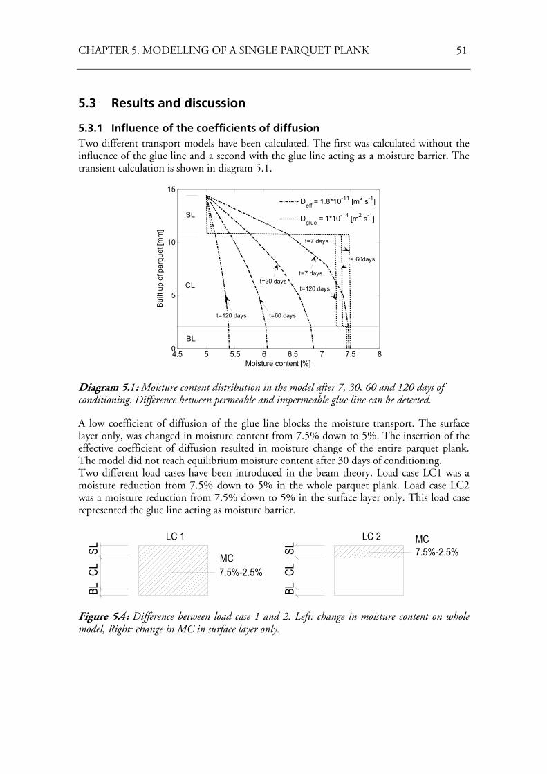
CHAPTER 5. MODELLING OF A SINGLE PARQUET PLANK 51
5.3 Results and discussion
5.3.1 Influence of the coefficients of diffusion Two different transport models have been calculated. The first was calculated without the influence of the glue line and a second with the glue line acting as a moisture barrier. The transient calculation is shown in diagram 5.1.
4.5 5 5.5 6 6.5 7 7.5 80
5
10
15
Moisture content [%]
Bui
lt up
of p
arqu
et [m
m]
Deff = 1.8*10-11 [m2 s-1]
Dglue = 1*10-14 [m2 s-1]
t=120 days t=60 days
t=30 dayst=7 days
SL
CL
BL
t=7 days
t= 60days
t=120 days
Diagram 5.1: Moisture content distribution in the model after 7, 30, 60 and 120 days of conditioning. Difference between permeable and impermeable glue line can be detected.
A low coefficient of diffusion of the glue line blocks the moisture transport. The surface layer only, was changed in moisture content from 7.5% down to 5%. The insertion of the effective coefficient of diffusion resulted in moisture change of the entire parquet plank. The model did not reach equilibrium moisture content after 30 days of conditioning. Two different load cases have been introduced in the beam theory. Load case LC1 was a moisture reduction from 7.5% down to 5% in the whole parquet plank. Load case LC2 was a moisture reduction from 7.5% down to 5% in the surface layer only. This load case represented the glue line acting as moisture barrier.
7.5%-2.5%
BLCL
SL
LC 17.5%-2.5%
LC 2
BLCL
SL
MC
MC
Figure 5.4: Difference between load case 1 and 2. Left: change in moisture content on whole model, Right: change in MC in surface layer only.
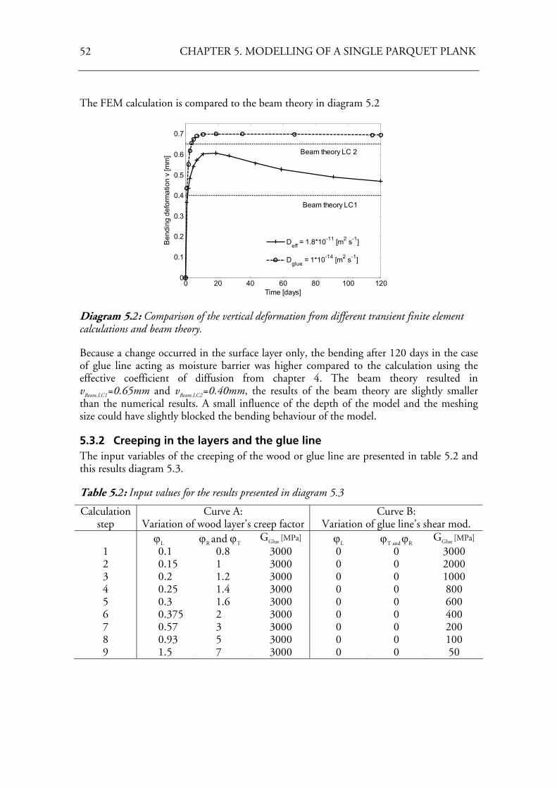
52 CHAPTER 5. MODELLING OF A SINGLE PARQUET PLANK
The FEM calculation is compared to the beam theory in diagram 5.2
0 20 40 60 80 100 1200
0.1
0.2
0.3
0.4
0.5
0.6
0.7
Time [days]
Ben
ding
def
orm
atio
n v
[mm
]
Deff = 1.8*10-11 [m2 s-1]
Dglue = 1*10-14 [m2 s-1]
Beam theory LC1
Beam theory LC 2
Diagram 5.2: Comparison of the vertical deformation from different transient finite element calculations and beam theory.
Because a change occurred in the surface layer only, the bending after 120 days in the case of glue line acting as moisture barrier was higher compared to the calculation using the effective coefficient of diffusion from chapter 4. The beam theory resulted in vBeam.LC1=0.65mm and vBeam.LC2=0.40mm, the results of the beam theory are slightly smaller than the numerical results. A small influence of the depth of the model and the meshing size could have slightly blocked the bending behaviour of the model.
5.3.2 Creeping in the layers and the glue line The input variables of the creeping of the wood or glue line are presented in table 5.2 and this results diagram 5.3.
Table 5.2: Input values for the results presented in diagram 5.3
Calculation step
Curve A: Variation of wood layer’s creep factor
Curve B: Variation of glue line’s shear mod.
ϕL ϕR and ϕT GGlue [MPa] ϕL ϕT and ϕR GGlue [MPa] 1 0.1 0.8 3000 0 0 3000 2 0.15 1 3000 0 0 2000 3 0.2 1.2 3000 0 0 1000 4 0.25 1.4 3000 0 0 800 5 0.3 1.6 3000 0 0 600 6 0.375 2 3000 0 0 400 7 0.57 3 3000 0 0 200 8 0.93 5 3000 0 0 100 9 1.5 7 3000 0 0 50
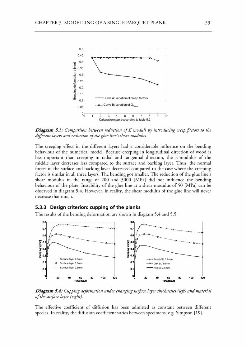
CHAPTER 5. MODELLING OF A SINGLE PARQUET PLANK 53
0 1 2 3 4 5 6 7 8 9 100
0.05
0.1
0.15
0.2
0.25
0.3
0.35
0.4
0.45
0.5
Calculation step acccording to table 5.2
Ben
ding
def
orm
atio
n v
[mm
]
Curve A: variation of creep factors
Curve B: variation of GGlue
Diagram 5.3: Comparison between reduction of E moduli by introducing creep factors to the different layers and reduction of the glue line’s shear modulus.
The creeping effect in the different layers had a considerable influence on the bending behaviour of the numerical model. Because creeping in longitudinal direction of wood is less important than creeping in radial and tangential direction, the E-modulus of the middle layer decreases less compared to the surface and backing layer. Thus, the normal forces in the surface and backing layer decreased compared to the case where the creeping factor is similar in all three layers. The bending got smaller. The reduction of the glue line’s shear modulus in the range of 200 and 3000 [MPa] did not influence the bending behaviour of the plate. Instability of the glue line at a shear modulus of 50 [MPa] can be observed in diagram 5.4. However, in reality, the shear modulus of the glue line will never decrease that much.
5.3.3 Design criterion: cupping of the planks The results of the bending deformation are shown in diagram 5.4 and 5.5.
0 20 40 60 80 100 1200
0.1
0.2
0.3
0.4
0.5
0.6
0.7
0.8
Time [days]
Cup
ping
v [m
m]
Surface layer 2.6mm
Surface layer 3.6mm
Surface layer 4.8mm
0 20 40 60 80 100 1200
0.1
0.2
0.3
0.4
0.5
0.6
0.7
0.8
Time [days]
Cup
ping
v [m
m]
Surface layer 4.8mm
Surface layer 3.6mm
Surface layer 2.6mm
0 20 40 60 80 100 1200
0.1
0.2
0.3
0.4
0.5
0.6
0.7
0.8
Time [days]
Cup
ping
v [m
m]
Surface layer 2.6mm
Surface layer 3.6mm
Surface layer 4.8mm
0 20 40 60 80 100 1200
0.1
0.2
0.3
0.4
0.5
0.6
0.7
0.8
Time [days]
Cup
ping
v [m
m]
Surface layer 4.8mm
Surface layer 3.6mm
Surface layer 2.6mm
0 20 40 60 80 100 1200
0.1
0.2
0.3
0.4
0.5
0.6
0.7
0.8
Time [days]
Cup
ping
v [m
m]
Beech
Oak
Ash
0 20 40 60 80 100 1200
0.1
0.2
0.3
0.4
0.5
0.6
0.7
0.8
Time [days]
Cup
ping
v [m
m]
Beech
Oak
Ash
0 20 40 60 80 100 1200
0.1
0.2
0.3
0.4
0.5
0.6
0.7
0.8
Time [days]
Cup
ping
v [m
m]
Beech
Oak
Ash
0 20 40 60 80 100 1200
0.1
0.2
0.3
0.4
0.5
0.6
0.7
0.8
Time [days]
Cup
ping
v [m
m]
Beech
Oak
Ash
0 20 40 60 80 100 1200
0.1
0.2
0.3
0.4
0.5
0.6
0.7
0.8
Time [days]
Cup
ping
v [m
m]
Beech SL 3.6mm
Oak SL 3.6mm
Ash SL 3.6mm
Diagram 5.4: Cupping deformation under changing surface layer thicknesses (left) and material of the surface layer (right).
The effective coefficient of diffusion has been admitted as constant between different species. In reality, the diffusion coefficient varies between specimens, e.g. Simpson [19].
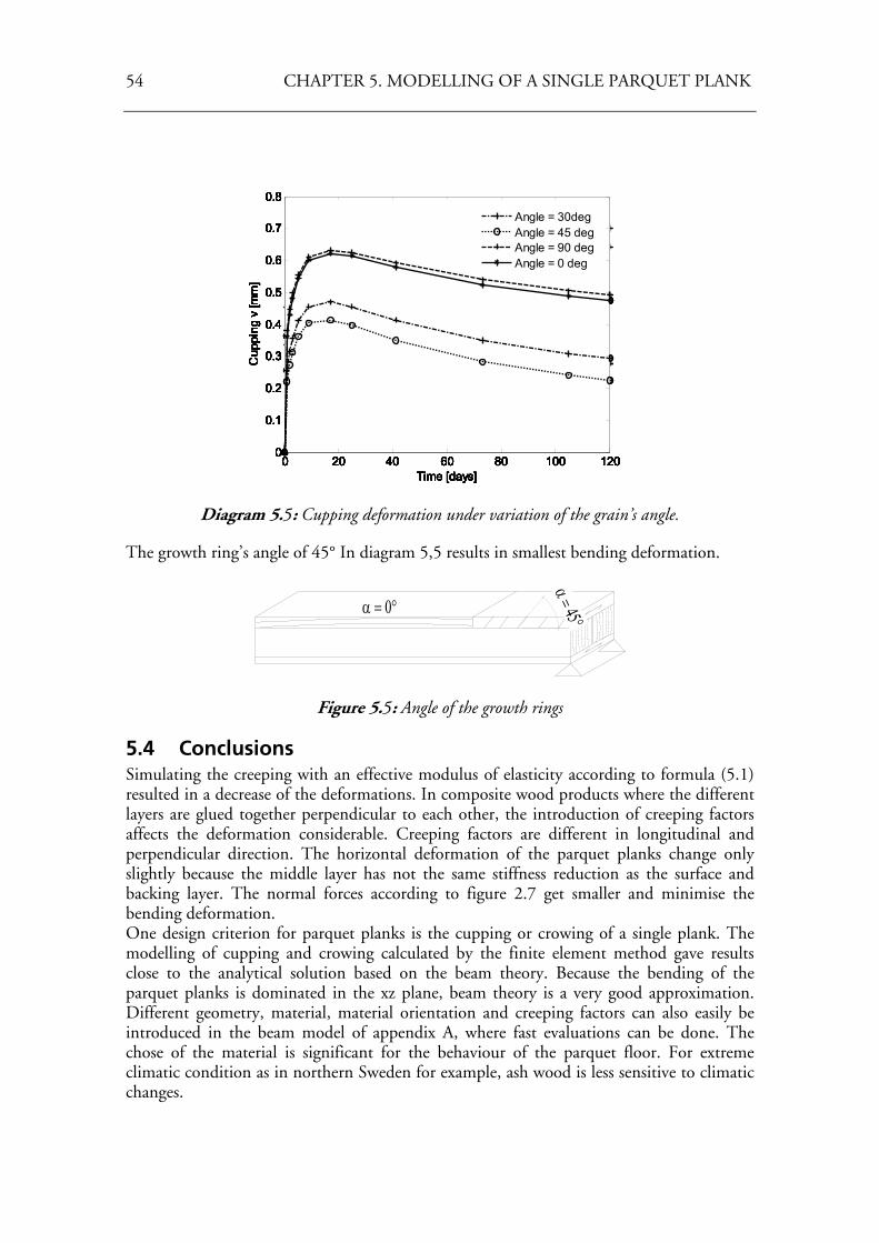
54 CHAPTER 5. MODELLING OF A SINGLE PARQUET PLANK
0 20 40 60 80 100 1200
0.1
0.2
0.3
0.4
0.5
0.6
0.7
0.8
Time [days]
Cup
ping
v [m
m]
Beech
Oak
Ash
0 20 40 60 80 100 1200
0.1
0.2
0.3
0.4
0.5
0.6
0.7
0.8
Time [days]
Cup
ping
v [m
m]
Beech
Oak
Ash
0 20 40 60 80 100 1200
0.1
0.2
0.3
0.4
0.5
0.6
0.7
0.8
Time [days]
Cup
ping
v [m
m]
Beech
Oak
Ash
0 20 40 60 80 100 1200
0.1
0.2
0.3
0.4
0.5
0.6
0.7
0.8
Time [days]
Cup
ping
v [m
m]
Beech
Oak
Ash
0 20 40 60 80 100 1200
0.1
0.2
0.3
0.4
0.5
0.6
0.7
0.8
Time [days]
Cup
ping
v [m
m]
Beech SL 3.6mm
Oak SL 3.6mm
Ash SL 3.6mm
0 20 40 60 80 100 1200
0.1
0.2
0.3
0.4
0.5
0.6
0.7
0.8
Time [days]
Cup
ping
v [m
m]
Angle = 30degAngle = 45 degAngle = 0 degAngle = 90 deg
0 20 40 60 80 100 1200
0.1
0.2
0.3
0.4
0.5
0.6
0.7
0.8
Time [days]
Cup
ping
v [m
m]
Angle = 30degAngle = 45 degAngle = 0 degAngle = 90 deg
0 20 40 60 80 100 1200
0.1
0.2
0.3
0.4
0.5
0.6
0.7
0.8
Time [days]
Cup
ping
v [m
m]
Angle = 30degAngle = 45 degAngle = 90 degAngle = 0 deg
0 20 40 60 80 100 1200
0.1
0.2
0.3
0.4
0.5
0.6
0.7
0.8
Time [days]
Cup
ping
v [m
m]
0 20 40 60 80 100 1200
0.1
0.2
0.3
0.4
0.5
0.6
0.7
0.8
Time [days]
Cup
ping
v [m
m]
Angle = 30degAngle = 45 degAngle = 90 degAngle = 0 deg
Diagram 5.5: Cupping deformation under variation of the grain’s angle.
The growth ring’s angle of 45° In diagram 5,5 results in smallest bending deformation.
α = 45°α = 0°
Figure 5.5: Angle of the growth rings
5.4 Conclusions Simulating the creeping with an effective modulus of elasticity according to formula (5.1) resulted in a decrease of the deformations. In composite wood products where the different layers are glued together perpendicular to each other, the introduction of creeping factors affects the deformation considerable. Creeping factors are different in longitudinal and perpendicular direction. The horizontal deformation of the parquet planks change only slightly because the middle layer has not the same stiffness reduction as the surface and backing layer. The normal forces according to figure 2.7 get smaller and minimise the bending deformation. One design criterion for parquet planks is the cupping or crowing of a single plank. The modelling of cupping and crowing calculated by the finite element method gave results close to the analytical solution based on the beam theory. Because the bending of the parquet planks is dominated in the xz plane, beam theory is a very good approximation. Different geometry, material, material orientation and creeping factors can also easily be introduced in the beam model of appendix A, where fast evaluations can be done. The chose of the material is significant for the behaviour of the parquet floor. For extreme climatic condition as in northern Sweden for example, ash wood is less sensitive to climatic changes.
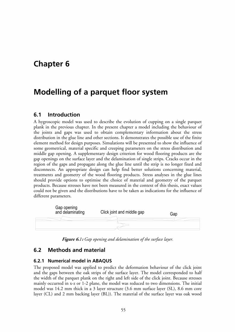
55
Chapter 6
Modelling of a parquet floor system
6.1 Introduction A hygroscopic model was used to describe the evolution of cupping on a single parquet plank in the previous chapter. In the present chapter a model including the behaviour of the joints and gaps was used to obtain complementary information about the stress distribution in the glue line and other sections. It demonstrates the possible use of the finite element method for design purposes. Simulations will be presented to show the influence of some geometrical, material specific and creeping parameters on the stress distribution and middle gap opening. A supplementary design criterion for wood flooring products are the gap openings on the surface layer and the delamination of single strips. Cracks occur in the region of the gaps and propagate along the glue line until the strip is no longer fixed and disconnects. An appropriate design can help find better solutions concerning material, treatments and geometry of the wood flooring products. Stress analyses in the glue lines should provide options to optimise the choice of material and geometry of the parquet products. Because stresses have not been measured in the context of this thesis, exact values could not be given and the distributions have to be taken as indications for the influence of different parameters.
GapClick joint and middle gapGap openingand delaminating
Figure 6.1: Gap opening and delamination of the surface layer.
6.2 Methods and material
6.2.1 Numerical model in ABAQUS The proposed model was applied to predict the deformation behaviour of the click joint and the gaps between the oak strips of the surface layer. The model corresponded to half the width of the parquet plank on the right and left side of the click joint. Because stresses mainly occurred in x-z or 1-2 plane, the model was reduced to two dimensions. The initial model was 14.2 mm thick in a 3 layer structure (3.6 mm surface layer (SL), 8.6 mm core layer (CL) and 2 mm backing layer (BL)). The material of the surface layer was oak wood
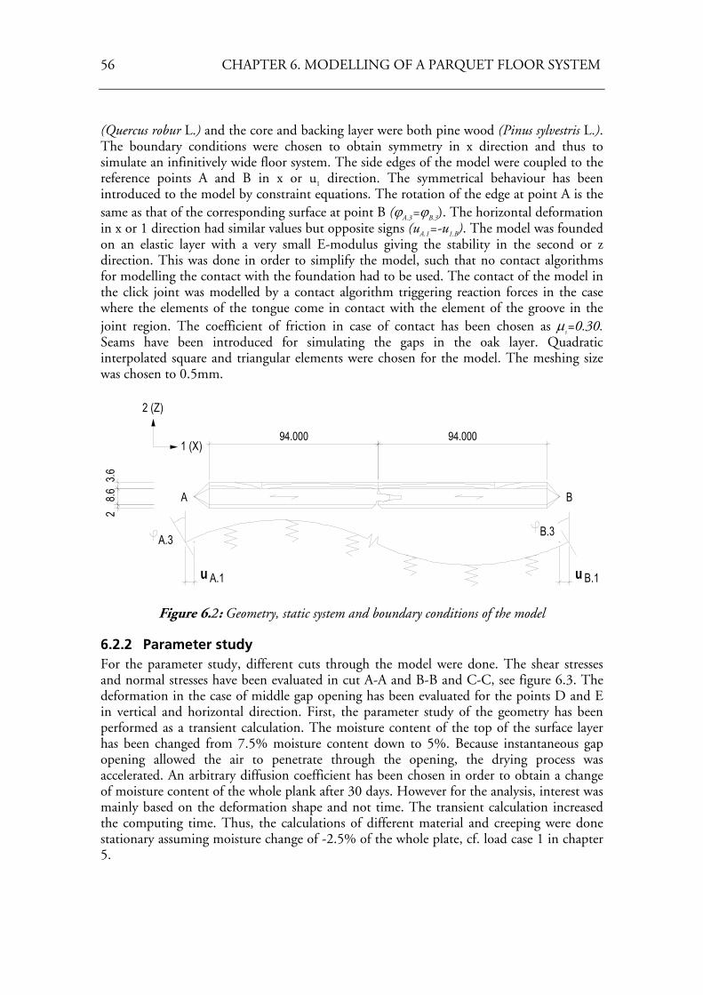
56 CHAPTER 6. MODELLING OF A PARQUET FLOOR SYSTEM
(Quercus robur L.) and the core and backing layer were both pine wood (Pinus sylvestris L.). The boundary conditions were chosen to obtain symmetry in x direction and thus to simulate an infinitively wide floor system. The side edges of the model were coupled to the reference points A and B in x or u1 direction. The symmetrical behaviour has been introduced to the model by constraint equations. The rotation of the edge at point A is the same as that of the corresponding surface at point B (ϕA.3=ϕB.3). The horizontal deformation in x or 1 direction had similar values but opposite signs (uA.1=-u1.B). The model was founded on an elastic layer with a very small E-modulus giving the stability in the second or z direction. This was done in order to simplify the model, such that no contact algorithms for modelling the contact with the foundation had to be used. The contact of the model in the click joint was modelled by a contact algorithm triggering reaction forces in the case where the elements of the tongue come in contact with the element of the groove in the joint region. The coefficient of friction in case of contact has been chosen as μs=0.30. Seams have been introduced for simulating the gaps in the oak layer. Quadratic interpolated square and triangular elements were chosen for the model. The meshing size was chosen to 0.5mm.
94.000 94.000
28.
63.
6
A B
u B.1A.1u
B.3A.3
1 (X)
2 (Z)
Figure 6.2: Geometry, static system and boundary conditions of the model
6.2.2 Parameter study For the parameter study, different cuts through the model were done. The shear stresses and normal stresses have been evaluated in cut A-A and B-B and C-C, see figure 6.3. The deformation in the case of middle gap opening has been evaluated for the points D and E in vertical and horizontal direction. First, the parameter study of the geometry has been performed as a transient calculation. The moisture content of the top of the surface layer has been changed from 7.5% moisture content down to 5%. Because instantaneous gap opening allowed the air to penetrate through the opening, the drying process was accelerated. An arbitrary diffusion coefficient has been chosen in order to obtain a change of moisture content of the whole plank after 30 days. However for the analysis, interest was mainly based on the deformation shape and not time. The transient calculation increased the computing time. Thus, the calculations of different material and creeping were done stationary assuming moisture change of -2.5% of the whole plate, cf. load case 1 in chapter 5.
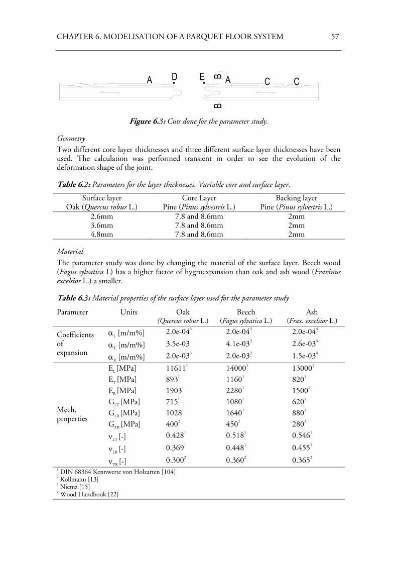
CHAPTER 6. MODELISATION OF A PARQUET FLOOR SYSTEM 57
A ABD
B
E CC
Figure 6.3: Cuts done for the parameter study.
Geometry Two different core layer thicknesses and three different surface layer thicknesses have been used. The calculation was performed transient in order to see the evolution of the deformation shape of the joint.
Table 6.2: Parameters for the layer thicknesses. Variable core and surface layer.
Surface layer Oak (Quercus robur L.)
Core Layer Pine (Pinus sylvestris L.)
Backing layer Pine (Pinus sylvestris L.)
2.6mm 7.8 and 8.6mm 2mm 3.6mm 7.8 and 8.6mm 2mm 4.8mm 7.8 and 8.6mm 2mm
Material The parameter study was done by changing the material of the surface layer. Beech wood (Fagus sylvatica L) has a higher factor of hygroexpansion than oak and ash wood (Fraxinus excelsior L.) a smaller.
Table 6.3: Material properties of the surface layer used for the parameter study
Parameter Units Oak (Quercus robur L.)
Beech (Fagus sylvatica L.)
Ash (Frax. excelsior L.)
αL [m/m%] 2.0e-043 2.0e-043 2.0e-044
αT [m/m%] 3.5e-03 4.1e-033 2.6e-034 Coefficients of expansion αR [m/m%] 2.0e-033 2.0e-033 1.5e-034
EL [MPa] 116111 140001 130001
ET [MPa] 8931 11601 8201
ER [MPa] 19031 22801 15001
GLT [MPa] 7151 10801 6201
GLR [MPa] 10281 16401 8801
GTR [MPa] 4002 4502 2802
νLT [-] 0.4281 0.5181 0.5461
νLR [-] 0.3691 0.4481 0.4551
Mech. properties
νTR [-] 0.3002 0.3602 0.3652 1 DIN 68364 Kennwerte von Holzarten [104] 2 Kollmann [13] 3 Niemz [15] 4 Wood Handbook [22]
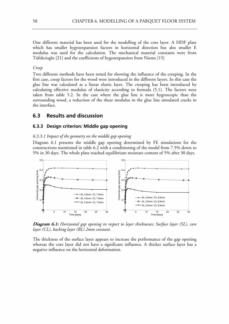
58 CHAPTER 6. MODELLING OF A PARQUET FLOOR SYSTEM
One different material has been used for the modelling of the core layer. A HDF plate which has smaller hygroexpansion factors in horizontal direction but also smaller E modulus was used for the calculation. The mechanical material constants were from Tüfekcioglu [21] and the coefficients of hygroexpansion from Niemz [15]
Creep Two different methods have been tested for showing the influence of the creeping. In the first case, creep factors for the wood were introduced in the different layers. In this case the glue line was calculated as a linear elastic layer. The creeping has been introduced by calculating effective modulus of elasticity according to formula (5.1). The factors were taken from table 5.2. In the case where the glue line is more hygroscopic than the surrounding wood, a reduction of the shear modulus in the glue line simulated cracks in the interface.
6.3 Results and discussion
6.3.3 Design criterion: Middle gap opening
6.3.3.1 Impact of the geometry on the middle gap opening Diagram 6.1 presents the middle gap opening determined by FE simulations for the constructions mentioned in table 6.2 with a conditioning of the model from 7.5% down to 5% in 30 days. The whole plate reached equilibrium moisture content of 5% after 30 days.
0 5 10 15 20 25 300
0.1
0.2
0.3
0.4
0.5
Time [days]
Hor
izon
tal g
ap o
peni
ng [m
m]
SL 4.8mm / CL 7.8mm
SL 3.6mm / CL 7.8mm
SL 2.6mm / CL 7.8mm
0 5 10 15 20 25 300
0.1
0.2
0.3
0.4
0.5
Time [days]
Hor
izon
tal g
ap o
peni
ng [m
m]
SL 4.8mm / CL 8.6mm
SL 3.6mm / CL 8.6mm
SL 2.6mm / CL 8.6mm
Diagram 6.1: Horizontal gap opening in respect to layer thicknesses; Surface layer (SL), core layer (CL), backing layer (BL) 2mm constant.
The thickness of the surface layer appears to increase the performance of the gap opening whereas the core layer did not have a significant influence. A thicker surface layer has a negative influence on the horizontal deformation.
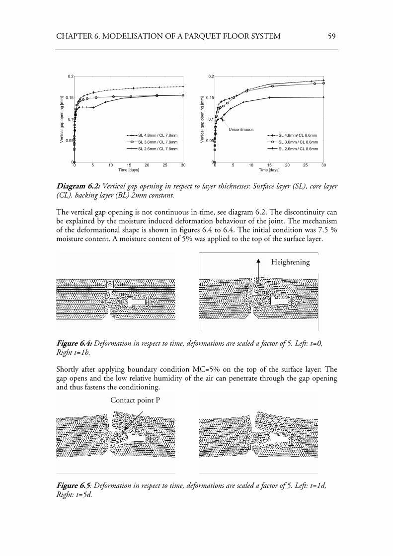
CHAPTER 6. MODELISATION OF A PARQUET FLOOR SYSTEM 59
0 5 10 15 20 25 300
0.05
0.1
0.15
0.2
Time [days]
Ver
tical
gap
ope
ning
[mm
]
SL 4.8mm / CL 7.8mm
SL 3.6mm / CL 7.8mm
SL 2.6mm / CL 7.8mm
0 5 10 15 20 25 300
0.05
0.1
0.15
0.2
Time [days]
Ver
tical
gap
ope
ning
[mm
]
SL 4.8mm/ CL 8.6mm
SL 3.6mm / CL 8.6mm
SL 2.6mm / CL 8.6mm
Uncontinuous
Diagram 6.2: Vertical gap opening in respect to layer thicknesses; Surface layer (SL), core layer (CL), backing layer (BL) 2mm constant.
The vertical gap opening is not continuous in time, see diagram 6.2. The discontinuity can be explained by the moisture induced deformation behaviour of the joint. The mechanism of the deformational shape is shown in figures 6.4 to 6.4. The initial condition was 7.5 % moisture content. A moisture content of 5% was applied to the top of the surface layer.
Figure 6.4: Deformation in respect to time, deformations are scaled a factor of 5. Left: t=0, Right t=1h.
Shortly after applying boundary condition MC=5% on the top of the surface layer: The gap opens and the low relative humidity of the air can penetrate through the gap opening and thus fastens the conditioning.
Figure 6.5: Deformation in respect to time, deformations are scaled a factor of 5. Left: t=1d, Right: t=5d.
Contact point P
Heightening
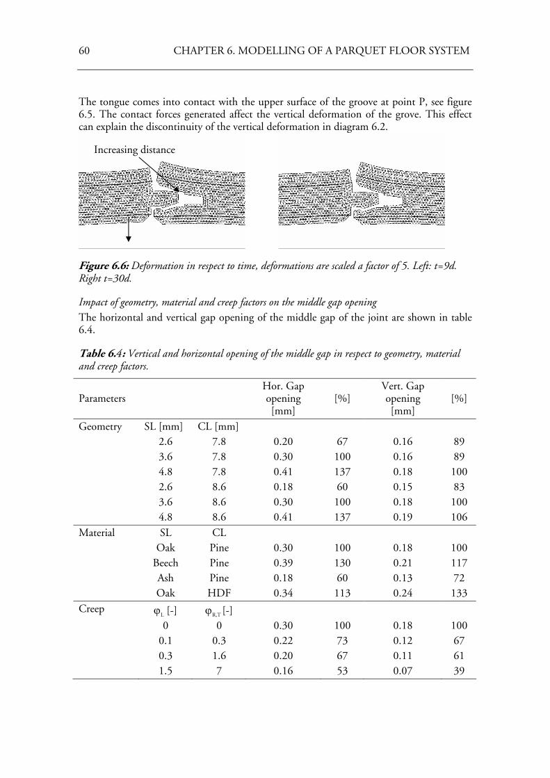
60 CHAPTER 6. MODELLING OF A PARQUET FLOOR SYSTEM
The tongue comes into contact with the upper surface of the groove at point P, see figure 6.5. The contact forces generated affect the vertical deformation of the grove. This effect can explain the discontinuity of the vertical deformation in diagram 6.2.
Figure 6.6: Deformation in respect to time, deformations are scaled a factor of 5. Left: t=9d. Right t=30d.
Impact of geometry, material and creep factors on the middle gap opening The horizontal and vertical gap opening of the middle gap of the joint are shown in table 6.4.
Table 6.4: Vertical and horizontal opening of the middle gap in respect to geometry, material and creep factors.
Parameters Hor. Gap opening [mm]
[%] Vert. Gap opening [mm]
[%]
Geometry SL [mm] CL [mm] 2.6 7.8 0.20 67 0.16 89 3.6 7.8 0.30 100 0.16 89 4.8 7.8 0.41 137 0.18 100 2.6 8.6 0.18 60 0.15 83 3.6 8.6 0.30 100 0.18 100 4.8 8.6 0.41 137 0.19 106
Material SL CL Oak Pine 0.30 100 0.18 100 Beech Pine 0.39 130 0.21 117 Ash Pine 0.18 60 0.13 72 Oak HDF 0.34 113 0.24 133
Creep ϕL [-] ϕR,T [-]
0 0 0.30 100 0.18 100 0.1 0.3 0.22 73 0.12 67 0.3 1.6 0.20 67 0.11 61 1.5 7 0.16 53 0.07 39
Increasing distance
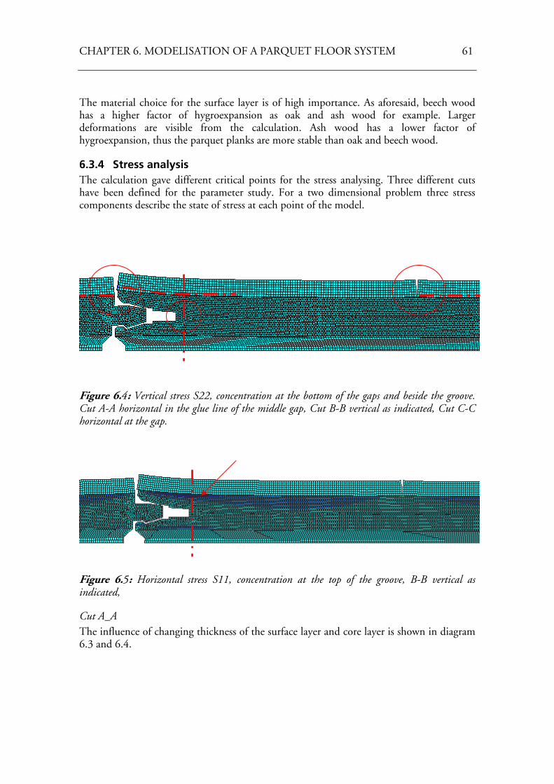
CHAPTER 6. MODELISATION OF A PARQUET FLOOR SYSTEM 61
The material choice for the surface layer is of high importance. As aforesaid, beech wood has a higher factor of hygroexpansion as oak and ash wood for example. Larger deformations are visible from the calculation. Ash wood has a lower factor of hygroexpansion, thus the parquet planks are more stable than oak and beech wood.
6.3.4 Stress analysis The calculation gave different critical points for the stress analysing. Three different cuts have been defined for the parameter study. For a two dimensional problem three stress components describe the state of stress at each point of the model.
Figure 6.4: Vertical stress S22, concentration at the bottom of the gaps and beside the groove. Cut A-A horizontal in the glue line of the middle gap, Cut B-B vertical as indicated, Cut C-C horizontal at the gap.
Figure 6.5: Horizontal stress S11, concentration at the top of the groove, B-B vertical as indicated,
Cut A_A The influence of changing thickness of the surface layer and core layer is shown in diagram 6.3 and 6.4.
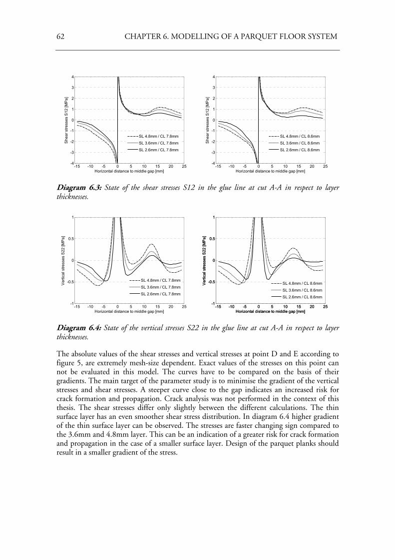
62 CHAPTER 6. MODELLING OF A PARQUET FLOOR SYSTEM
-15 -10 -5 0 5 10 15 20 25-4
-3
-2
-1
0
1
2
3
4
Horizontal distance to middle gap [mm]
She
ar s
tress
es S
12 [M
Pa]
SL 4.8mm / CL 7.8mm
SL 3.6mm / CL 7.8mm
SL 2.6mm / CL 7.8mm
-15 -10 -5 0 5 10 15 20 25-4
-3
-2
-1
0
1
2
3
4
Horizontal distance to middle gap [mm]
She
ar s
tress
es S
12 [M
Pa]
SL 4.8mm / CL 8.6mm
SL 3.6mm / CL 8.6mm
SL 2.6mm / CL 8.6mm
Diagram 6.3: State of the shear stresses S12 in the glue line at cut A-A in respect to layer thicknesses.
-15 -10 -5 0 5 10 15 20 25-1
-0.5
0
0.5
1
Horizontal distance to middle gap [mm]
Ver
tical
stre
sses
S22
[MP
a]
SL 4.8mm / CL 7.8mm
SL 3.6mm / CL 7.8mm
SL 2.6mm / CL 7.8mm
-15 -10 -5 0 5 10 15 20 25-1
-0.5
0
0.5
1
Horizontal distance to middle gap [mm]
Ver
tical
stre
sses
S22
[MP
a]
SL 4.8mm / CL 7.8mm
SL 3.6mm / CL 7.8mm
SL 2.6mm / CL 7.8mm
-15 -10 -5 0 5 10 15 20 25-1
-0.5
0
0.5
1
Horizontal distance to middle gap [mm]
Ver
tical
stre
sses
S22
[MP
a]
SL 4.8mm / CL 8.6mm
SL 3.6mm / CL 8.6mm
SL 2.6mm / CL 8.6mm
Diagram 6.4: State of the vertical stresses S22 in the glue line at cut A-A in respect to layer thicknesses.
The absolute values of the shear stresses and vertical stresses at point D and E according to figure 5, are extremely mesh-size dependent. Exact values of the stresses on this point can not be evaluated in this model. The curves have to be compared on the basis of their gradients. The main target of the parameter study is to minimise the gradient of the vertical stresses and shear stresses. A steeper curve close to the gap indicates an increased risk for crack formation and propagation. Crack analysis was not performed in the context of this thesis. The shear stresses differ only slightly between the different calculations. The thin surface layer has an even smoother shear stress distribution. In diagram 6.4 higher gradient of the thin surface layer can be observed. The stresses are faster changing sign compared to the 3.6mm and 4.8mm layer. This can be an indication of a greater risk for crack formation and propagation in the case of a smaller surface layer. Design of the parquet planks should result in a smaller gradient of the stress.
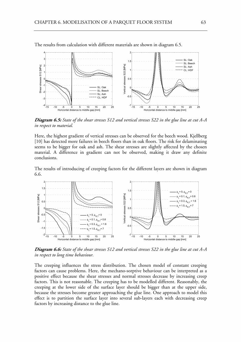
CHAPTER 6. MODELISATION OF A PARQUET FLOOR SYSTEM 63
The results from calculation with different materials are shown in diagram 6.5.
-15 -10 -5 0 5 10 15 20 25-4
-3
-2
-1
0
1
2
3
4
Horizontal distance to middle gap [mm]
She
ar s
tress
es S
12 [M
Pa]
SL: OakSL: BeechSL: AshCL: HDF
-15 -10 -5 0 5 10 15 20 25-1
-0.5
0
0.5
1
1.5
2
Horizontal distance to middle gap [mm]
Ver
tical
stre
sses
S22
[MP
a]
SL: OakSL: BeechSL: AshCL: HDF
Diagram 6.5: State of the shear stresses S12 and vertical stresses S22 in the glue line at cut A-A in respect to material.
Here, the highest gradient of vertical stresses can be observed for the beech wood. Kjellberg [10] has detected more failures in beech floors than in oak floors. The risk for delaminating seems to be bigger for oak and ash. The shear stresses are slightly affected by the chosen material. A difference in gradient can not be observed, making it draw any definite conclusions. The results of introducing of creeping factors for the different layers are shown in diagram 6.6.
-15 -10 -5 0 5 10 15 20 25-2
-1.5
-1
-0.5
0
0.5
1
1.5
2
Horizontal distance to middle gap [mm]
She
ar s
tress
es S
12 [M
Pa]
φL= 0, φR,T
= 0
φL= 0.1, φR,T
= 0.8
φL= 0.3, φR,T
= 1.6
φL= 1.5, φR,T
= 7
-15 -10 -5 0 5 10 15 20 25-1
-0.5
0
0.5
1
1.5
2
Horizontal distance to middle gap [mm]
Ver
tical
stre
sses
S22
[MP
a]
φL= 0, φR,T
= 0
φL= 0.1, φR,T
= 0.8
φL= 0.3, φR,T
= 1.6
φL= 1.5, φR,T
= 7
Diagram 6.6: State of the shear stresses S12 and vertical stresses S22 in the glue line at cut A-A in respect to long time behaviour.
The creeping influences the stress distribution. The chosen model of constant creeping factors can cause problems. Here, the mechano-sorptive behaviour can be interpreted as a positive effect because the shear stresses and normal stresses decrease by increasing creep factors. This is not reasonable. The creeping has to be modelled different. Reasonably, the creeping at the lower side of the surface layer should be bigger than at the upper side, because the stresses become greater approaching the glue line. One approach to model this effect is to partition the surface layer into several sub-layers each with decreasing creep factors by increasing distance to the glue line.
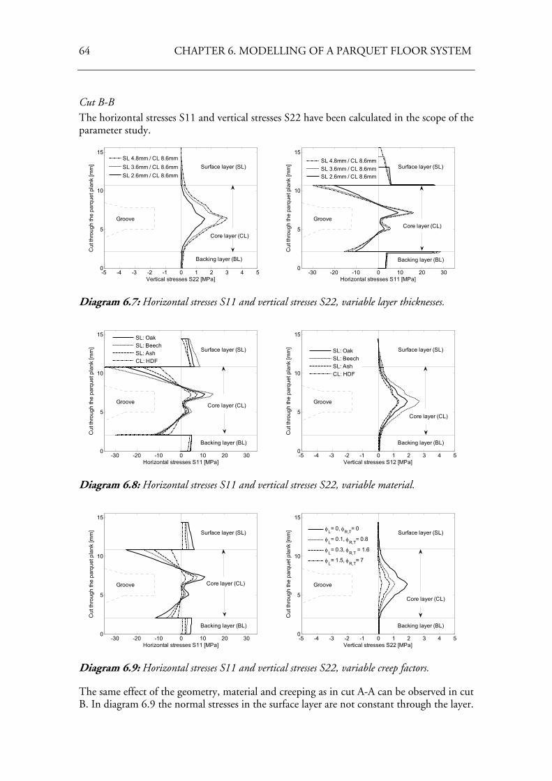
64 CHAPTER 6. MODELLING OF A PARQUET FLOOR SYSTEM
Cut B-B The horizontal stresses S11 and vertical stresses S22 have been calculated in the scope of the parameter study.
-5 -4 -3 -2 -1 0 1 2 3 4 50
5
10
15
Vertical stresses S22 [MPa]
Cut
thro
ugh
the
parq
uet p
lank
[mm
]
SL 4.8mm / CL 8.6mmSL 3.6mm / CL 8.6mmSL 2.6mm / CL 8.6mm
Surface layer (SL)
Core layer (CL)
Backing layer (BL)
Groove
-30 -20 -10 0 10 20 300
5
10
15
Horizontal stresses S11 [MPa]C
ut th
roug
h th
e pa
rque
t pla
nk [m
m] SL 4.8mm / CL 8.6mm
SL 3.6mm / CL 8.6mmSL 2.6mm / CL 8.6mm
Surface layer (SL)
Core layer (CL)
Backing layer (BL)
Groove
Diagram 6.7: Horizontal stresses S11 and vertical stresses S22, variable layer thicknesses.
-30 -20 -10 0 10 20 300
5
10
15
Horizontal stresses S11 [MPa]
Cut
thro
ugh
the
parq
uet p
lank
[mm
]
SL: OakSL: BeechSL: AshCL: HDF
Surface layer (SL)
Core layer (CL)
Backing layer (BL)
Groove
-5 -4 -3 -2 -1 0 1 2 3 4 50
5
10
15
Vertical stresses S12 [MPa]
Cut
thro
ugh
the
parq
uet p
lank
[mm
] SL: OakSL: BeechSL: AshCL: HDF
Surface layer (SL)
Core layer (CL)
Backing layer (BL)
Groove
Diagram 6.8: Horizontal stresses S11 and vertical stresses S22, variable material.
-30 -20 -10 0 10 20 300
5
10
15
Horizontal stresses S11 [MPa]
Cut
thro
ugh
the
parq
uet p
lank
[mm
] Surface layer (SL)
Core layer (CL)
Backing layer (BL)
Groove
-5 -4 -3 -2 -1 0 1 2 3 4 50
5
10
15
Vertical stresses S22 [MPa]
Cut
thro
ugh
the
parq
uet p
lank
[mm
] φL= 0, φR,T
= 0
φL= 0.1, φR,T
= 0.8
φL= 0.3, φR,T
= 1.6
φL= 1.5, φR,T
= 7
Surface layer (SL)
Core layer (CL)
Backing layer (BL)
Groove
Diagram 6.9: Horizontal stresses S11 and vertical stresses S22, variable creep factors.
The same effect of the geometry, material and creeping as in cut A-A can be observed in cut B. In diagram 6.9 the normal stresses in the surface layer are not constant through the layer.
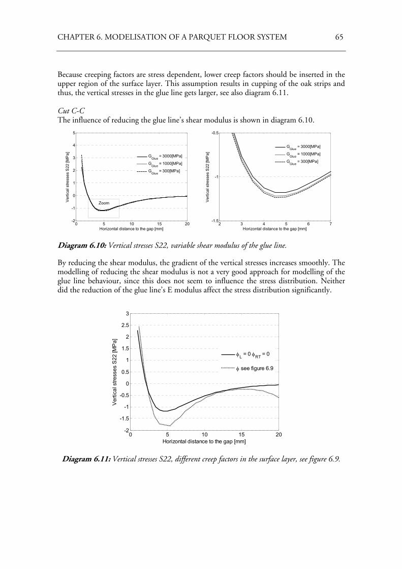
CHAPTER 6. MODELISATION OF A PARQUET FLOOR SYSTEM 65
Because creeping factors are stress dependent, lower creep factors should be inserted in the upper region of the surface layer. This assumption results in cupping of the oak strips and thus, the vertical stresses in the glue line gets larger, see also diagram 6.11. Cut C-C The influence of reducing the glue line’s shear modulus is shown in diagram 6.10.
0 5 10 15 20-2
-1
0
1
2
3
4
5
Horizontal distance to the gap [mm]
Ver
tical
stre
sses
S22
[MP
a] GGlue
= 3000[MPa]
GGlue
= 1000[MPa]
GGlue
= 300[MPa]
Zoom
2 3 4 5 6 7-1.5
-1
-0.5
Horizontal distance to the gap [mm]
Ver
tical
stre
sses
S22
[MP
a]
GGlue
= 3000[MPa]
GGlue
= 1000[MPa]
GGlue
= 300[MPa]
Diagram 6.10: Vertical stresses S22, variable shear modulus of the glue line.
By reducing the shear modulus, the gradient of the vertical stresses increases smoothly. The modelling of reducing the shear modulus is not a very good approach for modelling of the glue line behaviour, since this does not seem to influence the stress distribution. Neither did the reduction of the glue line’s E modulus affect the stress distribution significantly.
0 5 10 15 20-2
-1.5
-1
-0.5
0
0.5
1
1.5
2
2.5
3
Horizontal distance to the gap [mm]
Ver
tical
stre
sses
S22
[MP
a]
φL = 0 φRT = 0
φ see figure 6.9
Diagram 6.11: Vertical stresses S22, different creep factors in the surface layer, see figure 6.9.
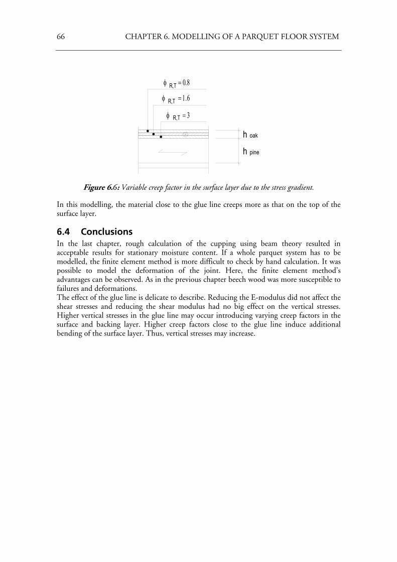
66 CHAPTER 6. MODELLING OF A PARQUET FLOOR SYSTEM
h
h
oak
pine
φ = 0.8R,T
φ = 1.6R,T
φ = 3R,T
Figure 6.6: Variable creep factor in the surface layer due to the stress gradient.
In this modelling, the material close to the glue line creeps more as that on the top of the surface layer.
6.4 Conclusions In the last chapter, rough calculation of the cupping using beam theory resulted in acceptable results for stationary moisture content. If a whole parquet system has to be modelled, the finite element method is more difficult to check by hand calculation. It was possible to model the deformation of the joint. Here, the finite element method’s advantages can be observed. As in the previous chapter beech wood was more susceptible to failures and deformations. The effect of the glue line is delicate to describe. Reducing the E-modulus did not affect the shear stresses and reducing the shear modulus had no big effect on the vertical stresses. Higher vertical stresses in the glue line may occur introducing varying creep factors in the surface and backing layer. Higher creep factors close to the glue line induce additional bending of the surface layer. Thus, vertical stresses may increase.
67
Chapter 7
Concluding remarks
7.1 Conclusions The work presented in this diploma thesis has resulted in many conclusions, which can be found in the corresponding sections and subsections. The aim of this chapter is to give a short overview of some general conclusions drawn. The finite element modelling has been tested for predicting different phenomena, which could be used for the design of wood flooring systems. The first such design criterion for parquet planks treated in the scope of this diploma thesis was the distortion of the planks. The finite element model used gave results similar to the analytical solution based on beam theory. However, in the case of including ductility in the glue layer and time dependent deformations, the beam model has some limitations and has to be complemented by finite element calculations. The relaxation of the different layers influences the bending deformation of the plate. For creeping as for relaxation, creeping factors are different in longitudinal or perpendicular direction. Thus, not only stresses but also deformations are affected by reducing the moduli of elasticity. In the case of long -term loading, the cupping and crowing effects are minimized by relaxation of the different layers. From the design perspective, results based on calculations with elastic properties without introducing creeping factors are on the safe side, i.e. larger deformations than experienced in practice are predicted. The growth ring orientation has a considerable influence on the deformation of the plate. An angle of 45° (between tangential direction and horizontal plane) in the surface layer minimized the cupping deformation. As expected, the bending of the parquet planks increase with increasing factor of hygroexpansion of the surface layer. Thus, parquet planks consisting of e.g. beech wood in the surface layer, are more sensitive than those consisting of ash wood for example, due to the fact that beech wood has a higher factor of hygroexpansion than ash wood. Design with a model of a whole parquet system helps finding optimal solutions in terms of stresses in the glue line and gap opening of the surface layer. Here, the finite element modelling has several advantages compared to traditionally testing. The time needed for calculation is much smaller compared to laboratory tests, although the results of the calculations must be validated by experiments. Other advantages include the possibility to optimize the geometry of the joint and the lay-up of the planks in a rather straightforward manner. The design process of wood flooring systems should include basic material testing, finite element analyses and, finally, testing of the developed product. It is also important to add that this design process ideally should be made iterative so that design issues, aesthetical
68 CHAPTER 7. CONCLUDING REMARKS
issues, production technology issues etc can be taken into account in a concurrent design approach. Being a sensitive part of the parquet system, the click joint has been tested extensively. The current investigation has shown that also the main factor of hygroexpansion has a considerable importance on the deformation shape and stress distribution. The material properties of the glue line and lacquer are difficult to determine, although the finite element method can be used for parameter estimation. Parameter studies help to better understand the behaviour of the glue-wood composite. The long time behaviour of the glue line did not considerably influence the deformation and stress distribution. It seems to be a good approach in terms of modelling to assign the UF resin layer properties making it less hygroscopic than wood and acting as a linear elastic layer. A hygroscopic material model may make more sense for the wood material than for the glue line. .
7.2 Proposal for future work Several material properties have been tested and used in the scope of this diploma thesis. The most important input factors are the factor of hygroexpansion and E-modulus in longitudinal, radial and tangential direction. The shear modulus and Poisson’s ratio do not have equally important influence on the deformational behaviour. The diffusion coefficients of the basic material were tested in the scope of this thesis. If the conditioning time of parquet planks is important, accurate modelling of the parquet’s time dependent deformation should be performed, and thus coefficients of diffusion in both horizontal and perpendicular directions are needed. Cyclic acclimatisation increases the relaxation in the different layers. Testing in cyclic climates can be performed to get more information about the long-term behaviour of the parquet planks. The samples need to be conditioned until equilibrium moisture content to ensure that a final stage has been reached. The residual stresses was set to zero for the finite element calculations, and measuring of residual stresses could thus provide more accurate initial conditions for the modelling. Additional tests on the parquet planks consisting of the determination of the coefficient of diffusion and hygroexpansion of the glue line and lacquer would help refining the moisture transport modelling. The model of a parquet floor system was not calibrated in the scope of this diploma thesis. Measuring and recording of gap openings close to the joint and between surface layer planks provides additional information for refining and calibrating the model. The stress comparison of the parameter study was based on gradients of the stress fields. The delaminating problem of the surface layer should be examined by introducing crack analyses in the glue line. Here, an approach based on fracture mechanics could be of interest.
69
Bibliography [1] ABAQUS: Analysis user’s manual.- ABAQUS, Inc., 2003 [2] Baronas R.; Ivanauskas F.; Juodeikienè I.; Kajalavicius A.: Modelling of moisture
movement in wood during outdoor storage. – In: Nonlinear Analysis: Modelling and control – v.6, no 2 (2001) – Pages 3-14
[3] Benham, P.P.; Crawford, R.J.; Armstrong, C.G.: Mechanics of engineering materials. – Longman, Harlow 1987
[4] Blanchet, P: Caractérisation du comportement des lames de planchet d’ingénierie. – Doctoral thesis, Université de Laval, Laval 2004
[5] Bodig, J.; Jane, A.: Mechanics of wood and wood composites. – Van Nostrand Reinhold, New York 1982
[6] Carslaw, H.S.; Jaeger J.C.: Conduction of Heat in Solids. – Oxford University Press, London 1959
[7] Eriksson, J.: Moisture transport and moisture induced distortions in timber. – Doctoral Thesis, Departement of Applied Mechanics, Chalmers University of Technology, Göteborg 2005
[8] Hagstrand P-O.; Mechanical analysis of melamine-formaldehyde composites - Doctoral Thesis, Departement of Polymeric Materials, Chalmers University of Technology, Göteborg 1999
[9] Hanhijärvi, A.: Modelling of creep deformation mechanisms in wood. – Dissertation, Technical Research Centre of Finland, Espoo 1995
[10] Kjellberg, A.: Lamellparkett på golvwärme. – Examansarbete, Kungl Tekniska Högskolan Stockholm 2005
[11] Koponen, H.: Dependences of moisture diffusion coefficients of wood and wooden panels on moisture content and wood properties. – In: Paperi ja Puu-Papper och trä (1984) – P. 740-745.
[12] Koc, P.; Houska M.: Characterisation of the sorptive properties of spruce wood by the inverse identification Method. – In: Holz als Roh und Werkstoff. – Berlin 60 (2002) – P.265-S.270
[13] Kollmann, F.: Technologie des Holzes und der Holzwerkstoffe 2.Auflage – Springer Verlag, Berlin, Heidelberg, New York, 1982
[14] Jönsson, J.: Moisture induced stresses in timber structures. – Doctoral Thesis, Report TVBK-1031, Division of Structural Engineering, Lund University 2005
[15] Niemz, P.: Physik des Holzes und der Holzwerkstoffe – DRW-Verlag Weinbrenner GmbH & Co., Leinfelden-Echterdingen 1993
[16] Ormarsson, S.: Numerical Analysis of Moisture-Related Distorsions in sawn timber. – Doctoral Thesis, Departement of Structural Mechanics, Chalmers University of Technology, Göteborg 1999
[17] Ottosen, N.; Petersson, H.: Introduction to the finite element method. – Prentice Hall Europe, Harlow 1992
[18] Sehlstedt, M.: Properties of solid wood responsing to drying and heat treatment. – Doctoral Thesis, Lulea University of Technology 2005
70 BIBLIOGRAPHY
[19] Simpson, W.T.: Determination and use of moisture diffusion coefficient to characterize drying of northern red oak (Quercus rubra) – In: Wood science and technology. – Springer 27 (1993) – P. 409-420
[20] Popov, E.: Mechanics of materials 2nd edition – Pretience-Hall International editions
[21] Tüfekcioglu Z.: Mechanical properties of laminate floor joints. – Master’s Dissertation, Report TVSM 5122, Division of Structural Mechanics, Lund University 2006
[22] Wood handbook: Wood as an engineering material. – USDA Forest Products Laboratory, Forest Laboratory, Wisconsin, USA, 1999
Standards [101] DIN 52182 (1976)
Prüfungen von Holz; Bestimmung der Rohdichte [102] DIN 52184 (1979)
Prüfungen von Holz; Bestimmung der Quellung und Schwindung [103] DIN 52186 (1978)
Prüfungen von Holz; Biegeversuch [104] DIN 68364 (1979) Kennwerte von Holzarten: Festigkeit, Elastizität, Resistenz
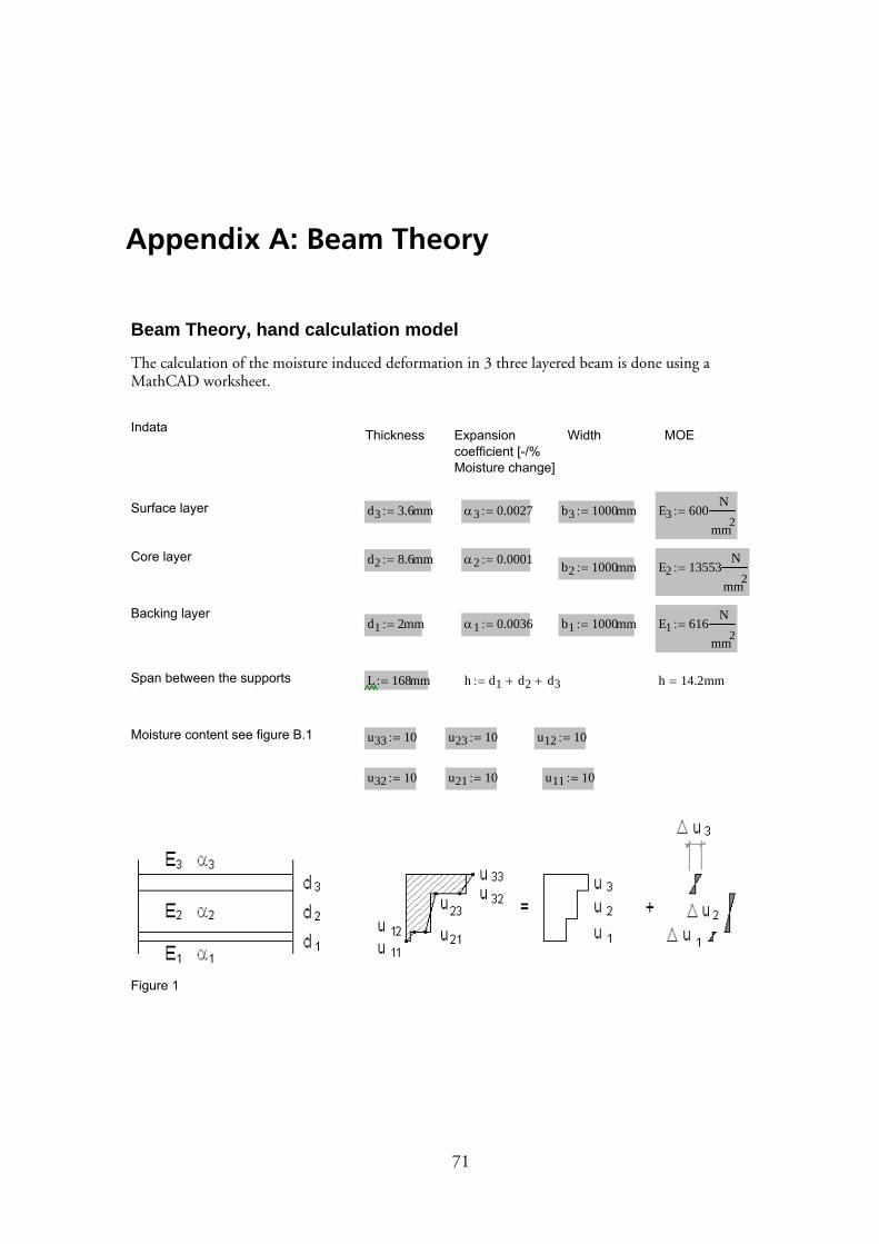
71
Appendix A: Beam Theory
Beam Theory, hand calculation model
The calculation of the moisture induced deformation in 3 three layered beam is done using aMathCAD worksheet.
Indata Thickness Expansioncoefficient [-/%Moisture change]
Width MOE
Surface layer d3 3.6mm:= α3 0.0027:= b3 1000mm:= E3 600
N
mm2:=
Core layer d2 8.6mm:= α2 0.0001:= b2 1000mm:= E2 13553N
mm2:=
Backing layerd1 2mm:= α1 0.0036:= b1 1000mm:= E1 616
N
mm2:=
Span between the supports L 168mm:= h d1 d2+ d3+:= h 14.2mm=
Moisture content see figure B.1 u33 10:= u23 10:= u12 10:=
u32 10:= u21 10:= u11 10:=
Figure 1
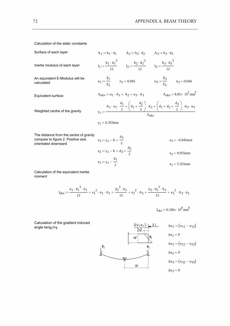
72 APPENDIX A. BEAM THEORY
Calculation of the static constants
Surface of each layer A1 b1 d1⋅:= A2 b2 d2⋅:= A3 b3 d3⋅:=
Inertie modulus of each layer I1b1 d1
3⋅
12:= I2
b2 d23
⋅
12:= I3
b3 d33
⋅
12:=
An equivalent E-Modulus will becalculated n1
E1
E2:= n1 0.045= n3
E3
E2:= n3 0.044=
Aekv n1 A1⋅ A2+ n3 A3⋅+:= Aekv 8.85 103× mm2
=Equivalent surface
Weighted centre of the gravity yc
A1 n1⋅d1
2⋅ d1
d2
2+
⎛⎜⎝
⎞⎟⎠
A2⋅+ d1 d2+d3
2+
⎛⎜⎝
⎞⎟⎠
A3⋅ n3⋅+
Aekv:=
yc 6.355mm=
The distance from the centre of gravity compare to figure 2. Positive axisorientated downward
e3 yc h−d3
2+:= e3 6.045− mm=
e2 yc h− d3+d2
2+:= e2 0.055mm=
e1 ycd1
2−:= e1 5.355mm=
Calculation of the equivalent inertiemoment
Iekvn1 d1
3⋅ b1⋅
12e1
2 n1⋅ A1⋅+d2
3 b2⋅
12+ e2
2 A2⋅+n3 d3
3⋅ b3⋅
12+ e3
2 A3⋅ n3⋅+:=
Iekv 6.166 104× mm4=
Calculation of the gradient inducedangle tan(φ)=φ Δu1 u11 u12−( ):=
Δu1 0=
Δu2 u21 u23−( ):=
Δu2 0=
Δu3 u32 u33−( ):=
Δu3 0=
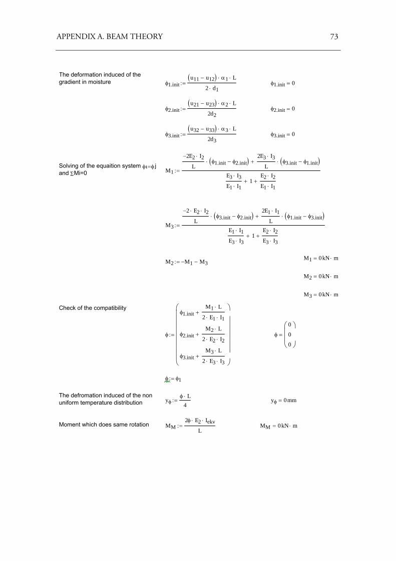
APPENDIX A. BEAM THEORY 73
The deformation induced of the gradient in moisture φ1.init
u11 u12−( ) α1⋅ L⋅
2 d1⋅:= φ1.init 0=
φ2.initu21 u23−( ) α2⋅ L⋅
2d2:= φ2.init 0=
φ3.initu32 u33−( ) α3⋅ L⋅
2d3:= φ3.init 0=
Solving of the equaition system φι=φ jand ΣMi=0 M1
2− E2 I2⋅
Lφ1.init φ2.init−( )⋅
2E3 I3⋅
Lφ3.init φ1.init−( )⋅+
E3 I3⋅
E1 I1⋅1+
E2 I2⋅
E1 I1⋅+
:=
M3
2− E2⋅ I2⋅
Lφ3.init φ2.init−( )⋅
2E1 I1⋅
Lφ1.init φ3.init−( )⋅+
E1 I1⋅
E3 I3⋅1+
E2 I2⋅
E3 I3⋅+
:=
M1 0kN m⋅=M2 M1− M3−:=
M2 0kN m⋅=
M3 0kN m⋅=
Check of the compatibility
φ
φ1.initM1 L⋅
2 E1⋅ I1⋅+
φ2.initM2 L⋅
2 E2⋅ I2⋅+
φ3.initM3 L⋅
2 E3⋅ I3⋅+
⎛⎜⎜⎜⎜⎜⎜⎜⎝
⎞⎟⎟⎟⎟⎟⎟⎟⎠
:= φ
0
0
0
⎛⎜⎜⎝
⎞⎟⎟⎠
=
φ φ1:=
The defromation induced of the nonuniform temperature distribution yφ
φ L⋅
4:= yφ 0mm=
Moment which does same rotation MM2φ E2⋅ Iekv⋅
L:= MM 0kN m⋅=
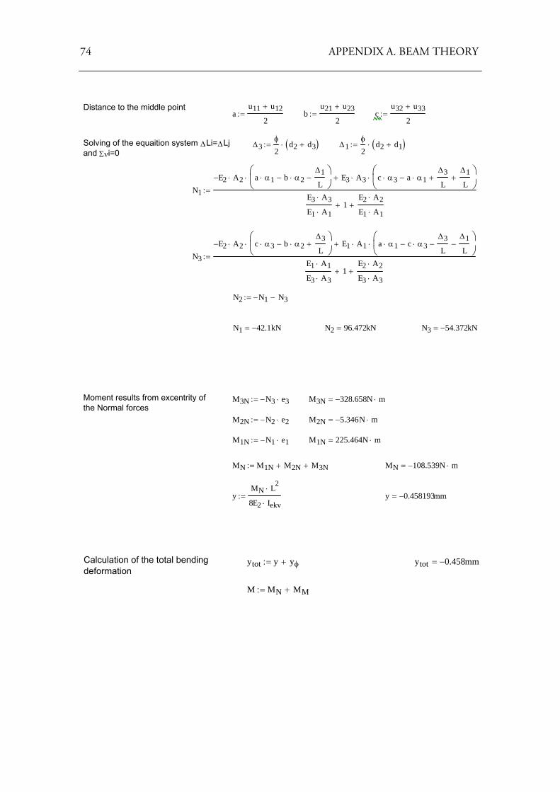
74 APPENDIX A. BEAM THEORY
Distance to the middle pointa
u11 u12+
2:= b
u21 u23+
2:= c
u32 u33+
2:=
Solving of the equaition system ΔLi=ΔLjand Σνi=0
Δ3φ
2d2 d3+( )⋅:= Δ1
φ
2d2 d1+( )⋅:=
N1
E2− A2⋅ a α1⋅ b α2⋅−Δ1
L−
⎛⎜⎝
⎞⎟⎠
⋅ E3 A3⋅ c α3⋅ a α1⋅−Δ3
L+
Δ1
L+
⎛⎜⎝
⎞⎟⎠
⋅+
E3 A3⋅
E1 A1⋅1+
E2 A2⋅
E1 A1⋅+
:=
N3
E2− A2⋅ c α3⋅ b α2⋅−Δ3
L+
⎛⎜⎝
⎞⎟⎠
⋅ E1 A1⋅ a α1⋅ c α3⋅−Δ3
L−
Δ1
L−
⎛⎜⎝
⎞⎟⎠
⋅+
E1 A1⋅
E3 A3⋅1+
E2 A2⋅
E3 A3⋅+
:=
N2 N1− N3−:=
N1 42.1− kN= N2 96.472kN= N3 54.372− kN=
Moment results from excentrity ofthe Normal forces
M3N N3− e3⋅:= M3N 328.658− N m⋅=
M2N N2− e2⋅:= M2N 5.346− N m⋅=
M1N N1− e1⋅:= M1N 225.464N m⋅=
MN M1N M2N+ M3N+:= MN 108.539− N m⋅=
yMN L2
⋅
8E2 Iekv⋅:= y 0.458193− mm=
Calculation of the total bendingdeformation
ytot y yφ+:= ytot 0.458− mm=
M MN MM+:=
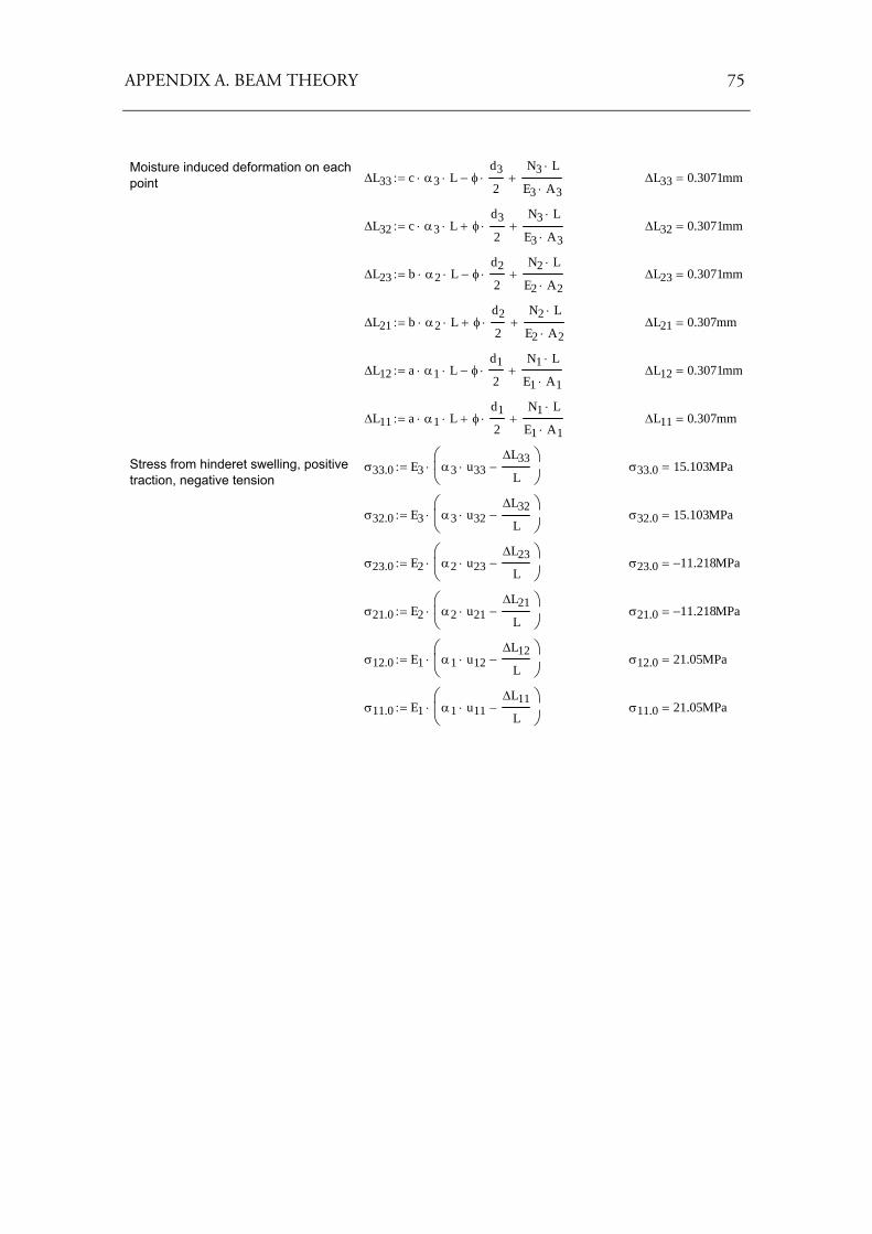
APPENDIX A. BEAM THEORY 75
Moisture induced deformation on eachpoint ΔL33 c α3⋅ L⋅ φ
d3
2⋅−
N3 L⋅
E3 A3⋅+:= ΔL33 0.3071mm=
ΔL32 c α3⋅ L⋅ φd3
2⋅+
N3 L⋅
E3 A3⋅+:= ΔL32 0.3071mm=
ΔL23 b α2⋅ L⋅ φd2
2⋅−
N2 L⋅
E2 A2⋅+:= ΔL23 0.3071mm=
ΔL21 b α2⋅ L⋅ φd2
2⋅+
N2 L⋅
E2 A2⋅+:= ΔL21 0.307mm=
ΔL12 a α1⋅ L⋅ φd1
2⋅−
N1 L⋅
E1 A1⋅+:= ΔL12 0.3071mm=
ΔL11 a α1⋅ L⋅ φd1
2⋅+
N1 L⋅
E1 A1⋅+:= ΔL11 0.307mm=
Stress from hinderet swelling, positivetraction, negative tension
σ33.0 E3 α3 u33⋅ΔL33
L−
⎛⎜⎝
⎞⎟⎠
⋅:= σ33.0 15.103MPa=
σ32.0 E3 α3 u32⋅ΔL32
L−
⎛⎜⎝
⎞⎟⎠
⋅:= σ32.0 15.103MPa=
σ23.0 E2 α2 u23⋅ΔL23
L−
⎛⎜⎝
⎞⎟⎠
⋅:= σ23.0 11.218− MPa=
σ21.0 E2 α2 u21⋅ΔL21
L−
⎛⎜⎝
⎞⎟⎠
⋅:= σ21.0 11.218− MPa=
σ12.0 E1 α1 u12⋅ΔL12
L−
⎛⎜⎝
⎞⎟⎠
⋅:= σ12.0 21.05MPa=
σ11.0 E1 α1 u11⋅ΔL11
L−
⎛⎜⎝
⎞⎟⎠
⋅:= σ11.0 21.05MPa=
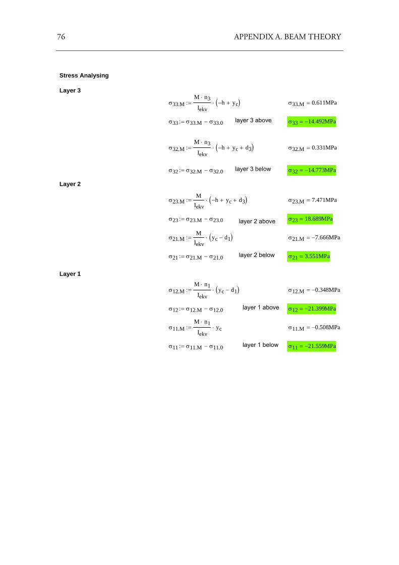
76 APPENDIX A. BEAM THEORY
Stress Analysing
Layer 3
σ33.MM n3⋅
Iekvh− yc+( )⋅:= σ33.M 0.611MPa=
σ33 σ33.M σ33.0−:= layer 3 above σ33 14.492− MPa=
σ32.MM n3⋅
Iekvh− yc+ d3+( )⋅:= σ32.M 0.331MPa=
σ32 σ32.M σ32.0−:= layer 3 below σ32 14.773− MPa=
Layer 2
σ23.MM
Iekvh− yc+ d3+( )⋅:= σ23.M 7.471MPa=
σ23 σ23.M σ23.0−:= σ23 18.689MPa=layer 2 above
σ21.MM
Iekvyc d1−( )⋅:= σ21.M 7.666− MPa=
σ21 σ21.M σ21.0−:= layer 2 below σ21 3.551MPa=
Layer 1
σ12.MM n1⋅
Iekvyc d1−( )⋅:= σ12.M 0.348− MPa=
σ12 σ12.M σ12.0−:= layer 1 above σ12 21.399− MPa=
σ11.MM n1⋅
Iekvyc⋅:= σ11.M 0.508− MPa=
σ11 σ11.M σ11.0−:= layer 1 below σ11 21.559− MPa=
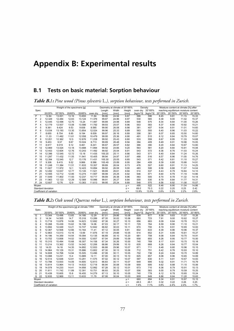
77
Appendix B: Experimental results
B.1 Tests on basic material: Sorption behaviour
Table B.1: Pine wood (Pinus sylvestris L.), sorption behaviour, tests performed in Zurich.
Length Width Height oven dry 20°/65%20/35% 20°/50% 20/65% 20/85% oven dry [mm] [mm] [mm] [kg/m^3] [kg/m^3] 20°/35% 20°/50% 20°/65% 20°/85%
P 1 12.84 13.001 13.16 13.655 11.84 99.86 24.94 8.87 566 596 8.45 9.81 11.15 15.33P 2 12.329 12.484 12.63 13.124 11.376 99.87 24.96 8.97 530 565 8.38 9.00 11.02 15.37P 3 12.445 12.598 12.75 13.24 11.487 99.89 24.98 8.89 548 575 8.34 8.84 11.00 15.26P 4 12.779 12.937 13.08 13.586 11.792 99.93 25.07 8.96 553 583 8.37 8.90 10.92 15.21P 5 9.361 9.424 9.53 9.838 8.585 99.90 26.08 8.98 381 407 9.04 8.91 11.01 14.60P 6 13.034 13.193 13.35 13.854 12.024 99.96 25.33 8.89 563 593 8.40 8.96 11.03 15.22P 7 8.655 8.754 8.85 9.194 8.009 99.97 26.16 8.89 358 381 8.07 8.85 10.50 14.80P 8 11.33 11.462 11.61 12.058 10.479 99.95 25.36 8.90 491 515 8.12 8.84 10.79 15.07P 9 12.201 12.362 12.5 12.876 11.228 99.92 25.43 8.80 533 559 8.67 8.95 11.33 14.68P 10 9.453 9.57 9.67 10.024 8.713 99.89 26.48 8.94 384 409 8.49 8.91 10.98 15.05P 11 8.917 9.019 9.12 9.461 8.241 99.87 26.57 8.82 366 390 8.20 8.84 10.67 14.80P 12 12.869 13.024 13.18 13.688 11.894 99.92 24.66 9.20 563 581 8.20 8.80 10.81 15.08P 13 12.453 12.604 12.76 13.243 11.492 99.92 25.04 8.91 543 572 8.36 8.76 11.03 15.24P 14 12.396 12.545 12.72 13.18 11.435 100.20 25.11 8.86 543 571 8.40 8.84 11.24 15.26P 15 11.297 11.432 11.55 11.941 10.405 99.94 24.97 8.97 488 516 8.57 8.96 11.00 14.76P 16 12.394 12.545 12.7 13.176 11.431 100.30 25.05 8.85 543 571 8.42 8.81 11.10 15.27P 17 9.306 9.415 9.52 9.866 8.586 100.49 25.89 8.95 384 409 8.39 8.80 10.88 14.91P 18 11.248 11.384 11.51 11.833 10.357 99.89 26.04 8.73 476 507 8.60 8.91 11.13 14.25P 19 11.827 11.972 12.1 12.423 10.894 99.92 26.59 9.00 483 506 8.56 8.88 11.07 14.04P 20 12.492 12.637 12.77 13.145 11.521 99.89 26.61 8.94 514 537 8.43 8.79 10.84 14.10P 21 12.555 12.712 12.85 13.274 11.557 99.99 25.25 8.92 546 571 8.64 8.79 11.19 14.86P 22 11.649 11.802 11.93 12.237 10.717 99.89 26.38 8.96 483 505 8.70 8.78 11.32 14.18P 23 11.963 12.123 12.29 12.569 10.996 99.91 26.27 8.84 500 530 8.79 8.84 11.77 14.31P 24 12.607 12.76 12.9 13.363 11.613 99.95 25.24 8.89 548 575 8.56 8.92 11.08 15.07
Moyen μ = 495 522 8.46 8.90 11.04 14.86Standard deviation σ = 69.0 70.3 0.22 0.20 0.25 0.42Coefficient of variation ν = 13.9% 13.5% 2.6% 2.3% 2.2% 2.8%
Density Moisture content at climate [%] after reaching equilibrium moisture contentSpec.
Weight of the specimens [g] Geometry at climate of 20°/65%
Table B.2: Oak wood (Quercus robur L.), sorption behaviour, tests performed in Zurich.
Length Width Height oven dry 20°/65%20/35% 20°/50% 20/65% 20/85% oven dry [mm] [mm] [mm] [kg/m^3] [kg/m^3] 20°/35% 20°/50% 20°/65% 20°/85%
Q 1 13.344 13.498 13.65 14.166 12.29 67.01 29.86 10.08 639 677 8.58 9.83 11.07 15.26Q 2 14.34 14.505 14.7 15.318 13.289 67.35 30.02 10.06 693 723 7.91 9.00 10.62 15.27Q 3 13.719 13.878 14.06 14.623 12.692 67.38 30.27 10.10 656 683 8.09 8.84 10.78 15.21Q 4 15.268 15.439 15.62 16.198 14.06 67.03 30.17 10.11 729 764 8.59 8.90 11.10 15.21Q 5 13.894 14.049 14.21 14.747 12.842 66.82 30.03 10.11 674 700 8.19 8.91 10.65 14.83Q 6 12.367 12.508 12.66 13.164 11.41 67.12 30.05 9.91 602 633 8.39 8.96 10.96 15.37Q 7 12.863 13.013 13.16 13.69 11.876 67.19 29.88 10.05 614 652 8.31 8.85 10.81 15.27Q 8 14.196 14.359 14.54 15.094 13.135 66.89 30.10 10.20 681 708 8.08 8.84 10.70 14.91Q 9 13.702 13.858 14.02 14.555 12.657 67.04 29.89 10.09 658 693 8.26 8.95 10.77 15.00Q 10 15.315 15.494 15.68 16.307 14.158 67.34 30.26 10.00 740 769 8.17 8.91 10.75 15.18Q 11 13.214 13.362 13.52 14.042 12.206 66.86 29.99 10.10 635 668 8.26 8.84 10.77 15.04Q 12 14.03 14.18 14.35 14.892 12.933 66.88 29.96 10.07 671 711 8.48 8.80 10.96 15.15Q 13 14.964 15.129 15.31 15.886 13.802 67.30 30.13 10.06 712 751 8.42 8.76 10.93 15.10Q 14 14.608 14.768 14.94 15.505 13.496 67.08 30.11 10.05 702 736 8.24 8.84 10.70 14.89Q 15 13.088 13.231 13.4 13.889 12.11 67.00 30.13 10.10 625 657 8.08 8.96 10.65 14.69Q 16 12.514 12.648 12.81 13.291 11.575 67.02 30.12 10.07 597 630 8.11 8.81 10.67 14.83Q 17 13.788 13.933 14.09 14.605 12.613 66.83 30.11 10.07 649 695 9.32 8.91 11.71 15.79Q 18 13.814 13.964 14.13 14.633 12.718 66.94 30.08 10.09 659 695 8.62 8.88 11.10 15.06Q 19 14.078 14.233 14.41 14.958 12.992 67.28 30.12 10.01 673 710 8.36 8.79 10.91 15.13Q 20 11.611 11.742 11.89 12.391 10.751 66.93 30.25 10.07 556 583 8.00 8.79 10.59 15.25Q 21 15.439 15.605 15.8 16.455 14.279 67.13 30.10 10.05 740 778 8.12 8.78 10.65 15.24Q 22 12.835 12.969 13.11 13.633 11.79 67.08 30.04 10.03 609 649 8.86 8.84 11.20 15.63
Moyen μ = 660 694 8.34 8.91 10.87 15.15Standard deviation σ = 48.5 49.1 0.32 0.22 0.26 0.25Coefficient of variation ν = 7.4% 7.1% 3.8% 2.4% 2.4% 1.7%
Spec.Weight of the specimens [g] at climate T/RH Geometry at climate of 20°/65% Density Moisture content at climate [%] after
reaching equilibrium moisture content
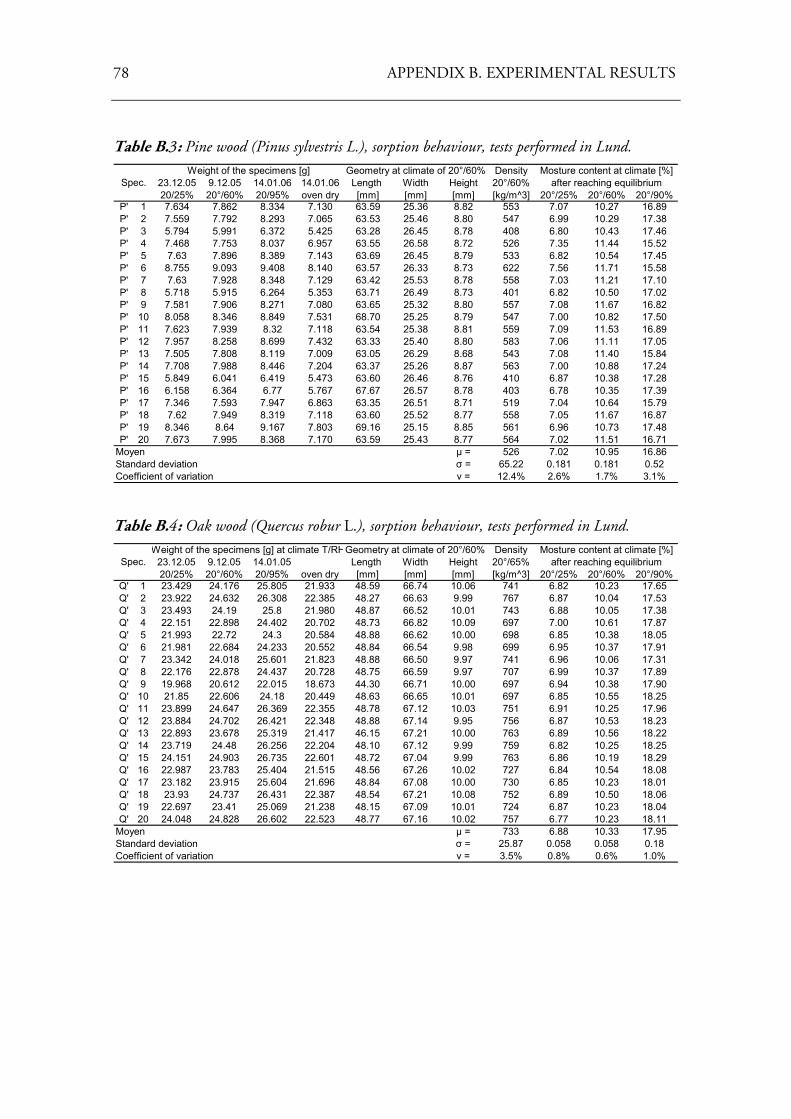
78 APPENDIX B. EXPERIMENTAL RESULTS
Table B.3: Pine wood (Pinus sylvestris L.), sorption behaviour, tests performed in Lund. Density
23.12.05 9.12.05 14.01.06 14.01.06 Length Width Height 20°/60%20/25% 20°/60% 20/95% oven dry [mm] [mm] [mm] [kg/m^3] 20°/25% 20°/60% 20°/90%
P' 1 7.634 7.862 8.334 7.130 63.59 25.36 8.82 553 7.07 10.27 16.89P' 2 7.559 7.792 8.293 7.065 63.53 25.46 8.80 547 6.99 10.29 17.38P' 3 5.794 5.991 6.372 5.425 63.28 26.45 8.78 408 6.80 10.43 17.46P' 4 7.468 7.753 8.037 6.957 63.55 26.58 8.72 526 7.35 11.44 15.52P' 5 7.63 7.896 8.389 7.143 63.69 26.45 8.79 533 6.82 10.54 17.45P' 6 8.755 9.093 9.408 8.140 63.57 26.33 8.73 622 7.56 11.71 15.58P' 7 7.63 7.928 8.348 7.129 63.42 25.53 8.78 558 7.03 11.21 17.10P' 8 5.718 5.915 6.264 5.353 63.71 26.49 8.73 401 6.82 10.50 17.02P' 9 7.581 7.906 8.271 7.080 63.65 25.32 8.80 557 7.08 11.67 16.82P' 10 8.058 8.346 8.849 7.531 68.70 25.25 8.79 547 7.00 10.82 17.50P' 11 7.623 7.939 8.32 7.118 63.54 25.38 8.81 559 7.09 11.53 16.89P' 12 7.957 8.258 8.699 7.432 63.33 25.40 8.80 583 7.06 11.11 17.05P' 13 7.505 7.808 8.119 7.009 63.05 26.29 8.68 543 7.08 11.40 15.84P' 14 7.708 7.988 8.446 7.204 63.37 25.26 8.87 563 7.00 10.88 17.24P' 15 5.849 6.041 6.419 5.473 63.60 26.46 8.76 410 6.87 10.38 17.28P' 16 6.158 6.364 6.77 5.767 67.67 26.57 8.78 403 6.78 10.35 17.39P' 17 7.346 7.593 7.947 6.863 63.35 26.51 8.71 519 7.04 10.64 15.79P' 18 7.62 7.949 8.319 7.118 63.60 25.52 8.77 558 7.05 11.67 16.87P' 19 8.346 8.64 9.167 7.803 69.16 25.15 8.85 561 6.96 10.73 17.48P' 20 7.673 7.995 8.368 7.170 63.59 25.43 8.77 564 7.02 11.51 16.71
Moyen μ = 526 7.02 10.95 16.86Standard deviation σ = 65.22 0.181 0.181 0.52Coefficient of variation ν = 12.4% 2.6% 1.7% 3.1%
Weight of the specimens [g] Mosture content at climate [%] after reaching equilibrium Spec.
Geometry at climate of 20°/60%
Table B.4: Oak wood (Quercus robur L.), sorption behaviour, tests performed in Lund. Geometry at climate of 20°/60% Density
23.12.05 9.12.05 14.01.05 Length Width Height 20°/65%20/25% 20°/60% 20/95% oven dry [mm] [mm] [mm] [kg/m^3] 20°/25% 20°/60% 20°/90%
Q' 1 23.429 24.176 25.805 21.933 48.59 66.74 10.06 741 6.82 10.23 17.65Q' 2 23.922 24.632 26.308 22.385 48.27 66.63 9.99 767 6.87 10.04 17.53Q' 3 23.493 24.19 25.8 21.980 48.87 66.52 10.01 743 6.88 10.05 17.38Q' 4 22.151 22.898 24.402 20.702 48.73 66.82 10.09 697 7.00 10.61 17.87Q' 5 21.993 22.72 24.3 20.584 48.88 66.62 10.00 698 6.85 10.38 18.05Q' 6 21.981 22.684 24.233 20.552 48.84 66.54 9.98 699 6.95 10.37 17.91Q' 7 23.342 24.018 25.601 21.823 48.88 66.50 9.97 741 6.96 10.06 17.31Q' 8 22.176 22.878 24.437 20.728 48.75 66.59 9.97 707 6.99 10.37 17.89Q' 9 19.968 20.612 22.015 18.673 44.30 66.71 10.00 697 6.94 10.38 17.90Q' 10 21.85 22.606 24.18 20.449 48.63 66.65 10.01 697 6.85 10.55 18.25Q' 11 23.899 24.647 26.369 22.355 48.78 67.12 10.03 751 6.91 10.25 17.96Q' 12 23.884 24.702 26.421 22.348 48.88 67.14 9.95 756 6.87 10.53 18.23Q' 13 22.893 23.678 25.319 21.417 46.15 67.21 10.00 763 6.89 10.56 18.22Q' 14 23.719 24.48 26.256 22.204 48.10 67.12 9.99 759 6.82 10.25 18.25Q' 15 24.151 24.903 26.735 22.601 48.72 67.04 9.99 763 6.86 10.19 18.29Q' 16 22.987 23.783 25.404 21.515 48.56 67.26 10.02 727 6.84 10.54 18.08Q' 17 23.182 23.915 25.604 21.696 48.84 67.08 10.00 730 6.85 10.23 18.01Q' 18 23.93 24.737 26.431 22.387 48.54 67.21 10.08 752 6.89 10.50 18.06Q' 19 22.697 23.41 25.069 21.238 48.15 67.09 10.01 724 6.87 10.23 18.04Q' 20 24.048 24.828 26.602 22.523 48.77 67.16 10.02 757 6.77 10.23 18.11
Moyen μ = 733 6.88 10.33 17.95Standard deviation σ = 25.87 0.058 0.058 0.18Coefficient of variation ν = 3.5% 0.8% 0.6% 1.0%
Spec.Weight of the specimens [g] at climate T/RH Mosture content at climate [%]
after reaching equilibrium
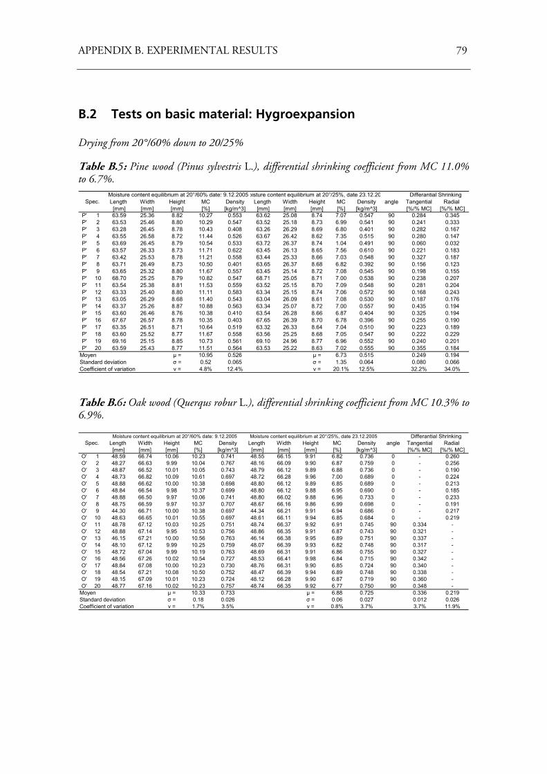
APPENDIX B. EXPERIMENTAL RESULTS 79
B.2 Tests on basic material: Hygroexpansion Drying from 20°/60% down to 20/25%
Table B.5: Pine wood (Pinus sylvestris L.), differential shrinking coefficient from MC 11.0% to 6.7%.
Length Width Height MC Density Length Width Height MC Density angle Tangential Radial [mm] [mm] [mm] [%] [kg/m^3] [mm] [mm] [mm] [%] [kg/m^3] [%/% MC] [%/% MC]
P' 1 63.59 25.36 8.82 10.27 0.553 63.62 25.08 8.74 7.07 0.547 90 0.284 0.345P' 2 63.53 25.46 8.80 10.29 0.547 63.52 25.18 8.73 6.99 0.541 90 0.241 0.333P' 3 63.28 26.45 8.78 10.43 0.408 63.26 26.29 8.69 6.80 0.401 90 0.282 0.167P' 4 63.55 26.58 8.72 11.44 0.526 63.67 26.42 8.62 7.35 0.515 90 0.280 0.147P' 5 63.69 26.45 8.79 10.54 0.533 63.72 26.37 8.74 1.04 0.491 90 0.060 0.032P' 6 63.57 26.33 8.73 11.71 0.622 63.45 26.13 8.65 7.56 0.610 90 0.221 0.183P' 7 63.42 25.53 8.78 11.21 0.558 63.44 25.33 8.66 7.03 0.548 90 0.327 0.187P' 8 63.71 26.49 8.73 10.50 0.401 63.65 26.37 8.68 6.82 0.392 90 0.156 0.123P' 9 63.65 25.32 8.80 11.67 0.557 63.45 25.14 8.72 7.08 0.545 90 0.198 0.155P' 10 68.70 25.25 8.79 10.82 0.547 68.71 25.05 8.71 7.00 0.538 90 0.238 0.207P' 11 63.54 25.38 8.81 11.53 0.559 63.52 25.15 8.70 7.09 0.548 90 0.281 0.204P' 12 63.33 25.40 8.80 11.11 0.583 63.34 25.15 8.74 7.06 0.572 90 0.168 0.243P' 13 63.05 26.29 8.68 11.40 0.543 63.04 26.09 8.61 7.08 0.530 90 0.187 0.176P' 14 63.37 25.26 8.87 10.88 0.563 63.34 25.07 8.72 7.00 0.557 90 0.435 0.194P' 15 63.60 26.46 8.76 10.38 0.410 63.54 26.28 8.66 6.87 0.404 90 0.325 0.194P' 16 67.67 26.57 8.78 10.35 0.403 67.65 26.39 8.70 6.78 0.396 90 0.255 0.190P' 17 63.35 26.51 8.71 10.64 0.519 63.32 26.33 8.64 7.04 0.510 90 0.223 0.189P' 18 63.60 25.52 8.77 11.67 0.558 63.56 25.25 8.68 7.05 0.547 90 0.222 0.229P' 19 69.16 25.15 8.85 10.73 0.561 69.10 24.96 8.77 6.96 0.552 90 0.240 0.201P' 20 63.59 25.43 8.77 11.51 0.564 63.53 25.22 8.63 7.02 0.555 90 0.355 0.184
Moyen μ = 10.95 0.526 μ = 6.73 0.515 0.249 0.194Standard deviation σ = 0.52 0.065 σ = 1.35 0.064 0.080 0.066Coefficient of variation ν = 4.8% 12.4% ν = 20.1% 12.5% 32.2% 34.0%
Spec.Moisture content equilibrium at 20°/60% date: 9.12.2005oisture content equilibrium at 20°/25%, date 23.12.20 Differantial Shrinking
Table B.6: Oak wood (Querqus robur L.), differential shrinking coefficient from MC 10.3% to 6.9%.
Length Width Height MC Density Length Width Height MC Density angle Tangential Radial [mm] [mm] [mm] [%] [kg/m^3] [mm] [mm] [mm] [%] [kg/m^3] [%/% MC] [%/% MC]
O' 1 48.59 66.74 10.06 10.23 0.741 48.55 66.15 9.91 6.82 0.736 0 - 0.260O' 2 48.27 66.63 9.99 10.04 0.767 48.16 66.09 9.90 6.87 0.759 0 - 0.256O' 3 48.87 66.52 10.01 10.05 0.743 48.79 66.12 9.89 6.88 0.736 0 - 0.190O' 4 48.73 66.82 10.09 10.61 0.697 48.72 66.28 9.96 7.00 0.689 0 - 0.224O' 5 48.88 66.62 10.00 10.38 0.698 48.80 66.12 9.89 6.85 0.689 0 - 0.213O' 6 48.84 66.54 9.98 10.37 0.699 48.80 66.12 9.88 6.95 0.690 0 - 0.185O' 7 48.88 66.50 9.97 10.06 0.741 48.80 66.02 9.88 6.96 0.733 0 - 0.233O' 8 48.75 66.59 9.97 10.37 0.707 48.67 66.16 9.86 6.99 0.698 0 - 0.191O' 9 44.30 66.71 10.00 10.38 0.697 44.34 66.21 9.91 6.94 0.686 0 - 0.217O' 10 48.63 66.65 10.01 10.55 0.697 48.61 66.11 9.94 6.85 0.684 0 - 0.219O' 11 48.78 67.12 10.03 10.25 0.751 48.74 66.37 9.92 6.91 0.745 90 0.334 -O' 12 48.88 67.14 9.95 10.53 0.756 48.86 66.35 9.91 6.87 0.743 90 0.321 -O' 13 46.15 67.21 10.00 10.56 0.763 46.14 66.38 9.95 6.89 0.751 90 0.337 -O' 14 48.10 67.12 9.99 10.25 0.759 48.07 66.39 9.93 6.82 0.748 90 0.317 -O' 15 48.72 67.04 9.99 10.19 0.763 48.69 66.31 9.91 6.86 0.755 90 0.327 -O' 16 48.56 67.26 10.02 10.54 0.727 48.53 66.41 9.98 6.84 0.715 90 0.342 -O' 17 48.84 67.08 10.00 10.23 0.730 48.76 66.31 9.90 6.85 0.724 90 0.340 -O' 18 48.54 67.21 10.08 10.50 0.752 48.47 66.39 9.94 6.89 0.748 90 0.338 -O' 19 48.15 67.09 10.01 10.23 0.724 48.12 66.28 9.90 6.87 0.719 90 0.360 -O' 20 48.77 67.16 10.02 10.23 0.757 48.74 66.35 9.92 6.77 0.750 90 0.348 -
Moyen μ = 10.33 0.733 μ = 6.88 0.725 0.336 0.219Standard deviation σ = 0.18 0.026 σ = 0.06 0.027 0.012 0.026Coefficient of variation ν = 1.7% 3.5% ν = 0.8% 3.7% 3.7% 11.9%
Spec.Moisture content equilibrium at 20°/60% date: 9.12.2005 Moisture content equilibrium at 20°/25%, date 23.12.2005 Differantial Shrinking
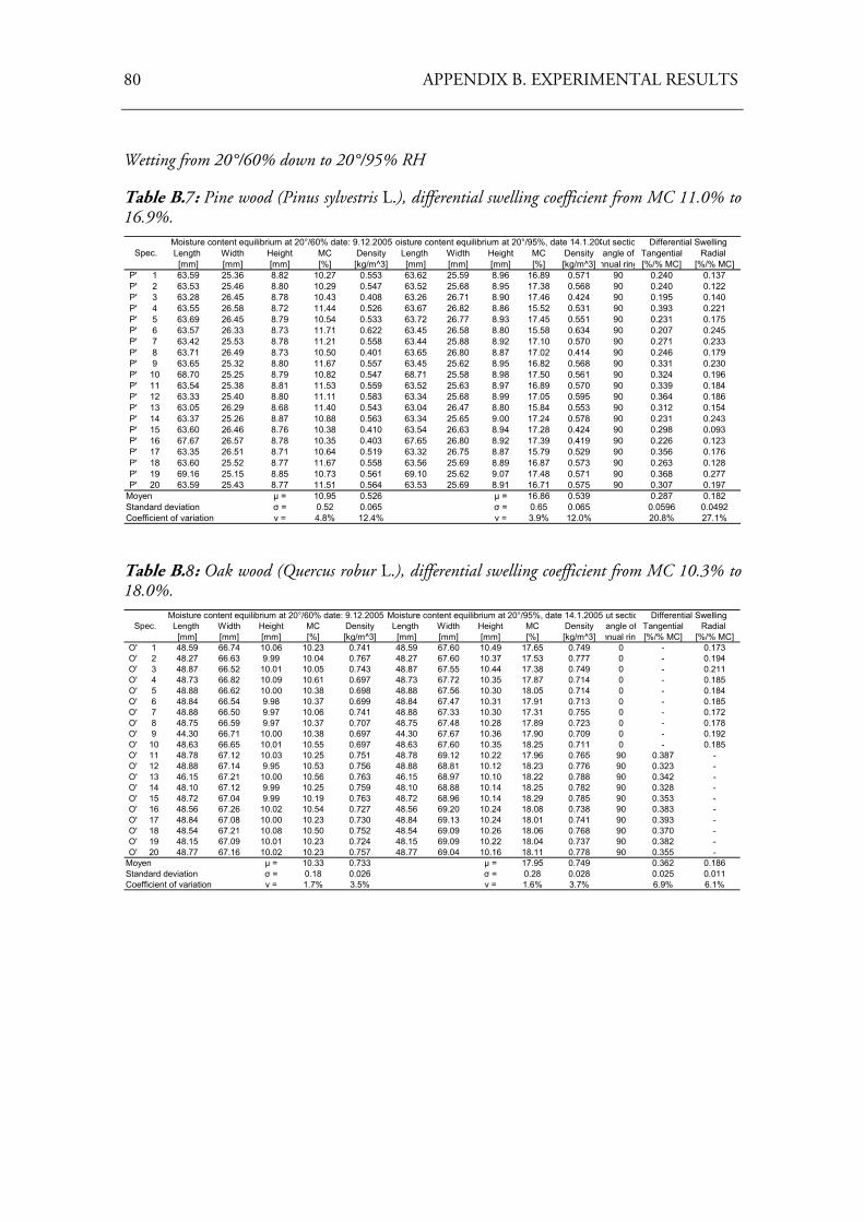
80 APPENDIX B. EXPERIMENTAL RESULTS
Wetting from 20°/60% down to 20°/95% RH
Table B.7: Pine wood (Pinus sylvestris L.), differential swelling coefficient from MC 11.0% to 16.9%.
Cut sectioLength Width Height MC Density Length Width Height MC Density angle of Tangential Radial [mm] [mm] [mm] [%] [kg/m^3] [mm] [mm] [mm] [%] [kg/m^3] nnual ring [%/% MC] [%/% MC]
P' 1 63.59 25.36 8.82 10.27 0.553 63.62 25.59 8.96 16.89 0.571 90 0.240 0.137P' 2 63.53 25.46 8.80 10.29 0.547 63.52 25.68 8.95 17.38 0.568 90 0.240 0.122P' 3 63.28 26.45 8.78 10.43 0.408 63.26 26.71 8.90 17.46 0.424 90 0.195 0.140P' 4 63.55 26.58 8.72 11.44 0.526 63.67 26.82 8.86 15.52 0.531 90 0.393 0.221P' 5 63.69 26.45 8.79 10.54 0.533 63.72 26.77 8.93 17.45 0.551 90 0.231 0.175P' 6 63.57 26.33 8.73 11.71 0.622 63.45 26.58 8.80 15.58 0.634 90 0.207 0.245P' 7 63.42 25.53 8.78 11.21 0.558 63.44 25.88 8.92 17.10 0.570 90 0.271 0.233P' 8 63.71 26.49 8.73 10.50 0.401 63.65 26.80 8.87 17.02 0.414 90 0.246 0.179P' 9 63.65 25.32 8.80 11.67 0.557 63.45 25.62 8.95 16.82 0.568 90 0.331 0.230P' 10 68.70 25.25 8.79 10.82 0.547 68.71 25.58 8.98 17.50 0.561 90 0.324 0.196P' 11 63.54 25.38 8.81 11.53 0.559 63.52 25.63 8.97 16.89 0.570 90 0.339 0.184P' 12 63.33 25.40 8.80 11.11 0.583 63.34 25.68 8.99 17.05 0.595 90 0.364 0.186P' 13 63.05 26.29 8.68 11.40 0.543 63.04 26.47 8.80 15.84 0.553 90 0.312 0.154P' 14 63.37 25.26 8.87 10.88 0.563 63.34 25.65 9.00 17.24 0.578 90 0.231 0.243P' 15 63.60 26.46 8.76 10.38 0.410 63.54 26.63 8.94 17.28 0.424 90 0.298 0.093P' 16 67.67 26.57 8.78 10.35 0.403 67.65 26.80 8.92 17.39 0.419 90 0.226 0.123P' 17 63.35 26.51 8.71 10.64 0.519 63.32 26.75 8.87 15.79 0.529 90 0.356 0.176P' 18 63.60 25.52 8.77 11.67 0.558 63.56 25.69 8.89 16.87 0.573 90 0.263 0.128P' 19 69.16 25.15 8.85 10.73 0.561 69.10 25.62 9.07 17.48 0.571 90 0.368 0.277P' 20 63.59 25.43 8.77 11.51 0.564 63.53 25.69 8.91 16.71 0.575 90 0.307 0.197
Moyen μ = 10.95 0.526 μ = 16.86 0.539 0.287 0.182Standard deviation σ = 0.52 0.065 σ = 0.65 0.065 0.0596 0.0492Coefficient of variation ν = 4.8% 12.4% ν = 3.9% 12.0% 20.8% 27.1%
Differential SwellingSpec.
Moisture content equilibrium at 20°/60% date: 9.12.2005 oisture content equilibrium at 20°/95%, date 14.1.200
Table B.8: Oak wood (Quercus robur L.), differential swelling coefficient from MC 10.3% to 18.0%.
Cut sectioLength Width Height MC Density Length Width Height MC Density angle of Tangential Radial [mm] [mm] [mm] [%] [kg/m^3] [mm] [mm] [mm] [%] [kg/m^3] nnual ring [%/% MC] [%/% MC]
O' 1 48.59 66.74 10.06 10.23 0.741 48.59 67.60 10.49 17.65 0.749 0 - 0.173O' 2 48.27 66.63 9.99 10.04 0.767 48.27 67.60 10.37 17.53 0.777 0 - 0.194O' 3 48.87 66.52 10.01 10.05 0.743 48.87 67.55 10.44 17.38 0.749 0 - 0.211O' 4 48.73 66.82 10.09 10.61 0.697 48.73 67.72 10.35 17.87 0.714 0 - 0.185O' 5 48.88 66.62 10.00 10.38 0.698 48.88 67.56 10.30 18.05 0.714 0 - 0.184O' 6 48.84 66.54 9.98 10.37 0.699 48.84 67.47 10.31 17.91 0.713 0 - 0.185O' 7 48.88 66.50 9.97 10.06 0.741 48.88 67.33 10.30 17.31 0.755 0 - 0.172O' 8 48.75 66.59 9.97 10.37 0.707 48.75 67.48 10.28 17.89 0.723 0 - 0.178O' 9 44.30 66.71 10.00 10.38 0.697 44.30 67.67 10.36 17.90 0.709 0 - 0.192O' 10 48.63 66.65 10.01 10.55 0.697 48.63 67.60 10.35 18.25 0.711 0 - 0.185O' 11 48.78 67.12 10.03 10.25 0.751 48.78 69.12 10.22 17.96 0.765 90 0.387 -O' 12 48.88 67.14 9.95 10.53 0.756 48.88 68.81 10.12 18.23 0.776 90 0.323 -O' 13 46.15 67.21 10.00 10.56 0.763 46.15 68.97 10.10 18.22 0.788 90 0.342 -O' 14 48.10 67.12 9.99 10.25 0.759 48.10 68.88 10.14 18.25 0.782 90 0.328 -O' 15 48.72 67.04 9.99 10.19 0.763 48.72 68.96 10.14 18.29 0.785 90 0.353 -O' 16 48.56 67.26 10.02 10.54 0.727 48.56 69.20 10.24 18.08 0.738 90 0.383 -O' 17 48.84 67.08 10.00 10.23 0.730 48.84 69.13 10.24 18.01 0.741 90 0.393 -O' 18 48.54 67.21 10.08 10.50 0.752 48.54 69.09 10.26 18.06 0.768 90 0.370 -O' 19 48.15 67.09 10.01 10.23 0.724 48.15 69.09 10.22 18.04 0.737 90 0.382 -O' 20 48.77 67.16 10.02 10.23 0.757 48.77 69.04 10.16 18.11 0.778 90 0.355 -
Moyen μ = 10.33 0.733 μ = 17.95 0.749 0.362 0.186Standard deviation σ = 0.18 0.026 σ = 0.28 0.028 0.025 0.011Coefficient of variation ν = 1.7% 3.5% ν = 1.6% 3.7% 6.9% 6.1%
Differential SwellingSpec.
Moisture content equilibrium at 20°/60% date: 9.12.2005 Moisture content equilibrium at 20°/95%, date 14.1.2005
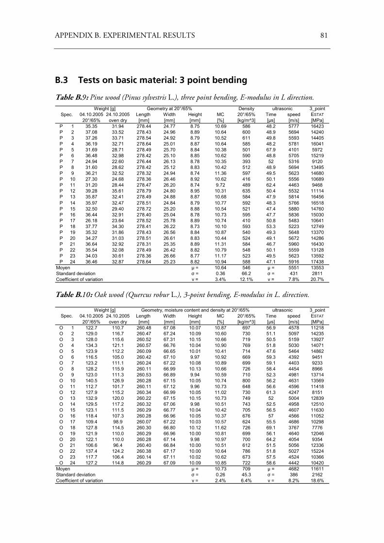
APPENDIX B. EXPERIMENTAL RESULTS 81
B.3 Tests on basic material: 3 point bending
Table B.9: Pine wood (Pinus sylvestris L.), three point bending, E-modulus in L direction. Density 3_point
04.10.2005 24.10.2005 Length Width Height MC 20°/65% Time speed ESTAT20°/65% oven dry [mm] [mm] [mm] [%] [kg/m^3] [μs] [m/s] [MPa]
P 1 35.35 31.94 278.44 24.77 8.75 10.69 586 48.2 5777 16423P 2 37.08 33.52 278.43 24.96 8.89 10.64 600 48.9 5694 14240P 3 37.26 33.71 278.54 24.92 8.79 10.52 611 49.8 5593 14405P 4 36.19 32.71 278.64 25.01 8.87 10.64 585 48.2 5781 16041P 5 31.69 28.71 278.49 25.70 8.84 10.38 501 67.9 4101 5972P 6 36.48 32.98 278.42 25.10 8.85 10.62 590 48.8 5705 15219P 7 24.94 22.60 276.44 26.13 8.78 10.35 393 52 5316 9120P 8 31.60 28.62 278.42 25.12 8.83 10.42 512 48.9 5694 13495P 9 36.21 32.52 278.32 24.94 8.74 11.36 597 49.5 5623 14680P 10 27.30 24.68 278.36 26.46 8.92 10.62 416 50.1 5556 10689P 11 31.20 28.44 278.47 26.20 8.74 9.72 489 62.4 4463 9468P 12 39.28 35.61 278.79 24.80 8.95 10.31 635 50.4 5532 11114P 13 35.87 32.41 278.49 24.88 8.87 10.68 584 47.9 5814 16456P 14 35.97 32.47 278.51 24.84 8.79 10.77 592 48.3 5766 16518P 15 32.50 29.40 278.72 25.20 8.88 10.54 521 47.4 5880 14760P 16 36.44 32.91 278.40 25.04 8.78 10.73 595 47.7 5836 15030P 17 26.18 23.64 278.52 25.78 8.89 10.74 410 50.8 5483 10641P 18 37.77 34.30 278.41 26.22 8.73 10.10 593 53.3 5223 12749P 19 35.32 31.86 278.43 26.56 8.84 10.87 540 49.3 5648 13370P 20 34.27 31.03 278.51 26.61 8.83 10.44 524 49.1 5672 14286P 21 36.64 32.92 278.31 25.35 8.89 11.31 584 46.7 5960 16430P 22 35.54 32.08 278.49 26.42 8.82 10.79 548 50.1 5559 13128P 23 34.03 30.61 278.36 26.66 8.77 11.17 523 49.5 5623 13592P 24 36.46 32.87 278.64 25.23 8.82 10.94 588 47.1 5916 17438
Moyen μ = 10.64 546 μ = 5551 13553Standard deviation σ = 0.36 66.2 σ = 431 2811Coefficient of variation ν = 3.4% 12.1% ν = 7.8% 20.7%
Geometry at 20°/65% ultrasonicWeight [g]Spec.
Table B.10: Oak wood (Quercus robur L.), 3-point bending, E-modulus in L. direction.
3_point04.10.2005 24.10.2005 Length Width Height MC 20°/65% Time speed ESTAT
20°/65% oven dry [mm] [mm] [mm] [%] [kg/m^3] [μs] [m/s] [MPa]O 1 122.7 110.7 260.48 67.08 10.07 10.87 697 56.9 4578 11218O 2 129.0 116.7 260.47 67.24 10.09 10.60 730 51.1 5097 14235O 3 128.0 115.6 260.52 67.31 10.15 10.66 719 50.5 5159 13927O 4 134.3 121.1 260.57 66.76 10.04 10.90 769 51.8 5030 14071O 5 123.9 112.2 260.09 66.65 10.01 10.41 714 47.6 5464 14862O 6 116.5 105.0 260.42 67.10 9.97 10.92 669 59.3 4392 9451O 7 123.2 111.1 260.24 67.22 10.08 10.89 699 59.1 4403 9233O 8 128.2 115.9 260.11 66.99 10.13 10.66 726 58.4 4454 8966O 9 123.0 111.3 260.53 66.89 9.94 10.59 710 52.3 4981 13714O 10 140.5 126.9 260.28 67.15 10.05 10.74 800 56.2 4631 13569O 11 112.7 101.7 260.11 67.12 9.96 10.73 648 56.6 4596 11418O 12 127.9 115.2 260.34 66.99 10.05 11.02 730 61.3 4247 8151O 13 132.9 120.0 260.22 67.15 10.15 10.73 749 52 5004 12839O 14 129.5 117.2 260.32 67.06 9.98 10.51 743 52.5 4958 12510O 15 123.1 111.5 260.29 66.77 10.04 10.42 705 56.5 4607 11630O 16 118.4 107.3 260.28 66.96 10.05 10.37 676 57 4566 11052O 17 109.4 98.9 260.07 67.22 10.03 10.57 624 55.5 4686 10298O 18 127.8 114.5 260.30 66.80 10.12 11.62 726 69.1 3767 7776O 19 121.9 110.0 260.29 66.96 10.00 10.81 699 56.1 4640 12046O 20 122.1 110.0 260.28 67.14 9.98 10.97 700 64.2 4054 9354O 21 106.6 96.4 260.40 66.84 10.00 10.51 612 51.5 5056 12336O 22 137.4 124.2 260.38 67.17 10.00 10.64 786 51.8 5027 15224O 23 117.7 106.4 260.14 67.11 10.02 10.62 673 57.5 4524 10366O 24 127.2 114.8 260.29 67.09 10.09 10.85 722 58.6 4442 10420
Moyen μ = 10.73 709 μ = 4682 11611Standard deviation σ = 0.26 45.3 σ = 386 2162Coefficient of variation ν = 2.4% 6.4% ν = 8.2% 18.6%
Spec.Weight [g] ultrasonicGeometry, moisture content and density at 20°/65%
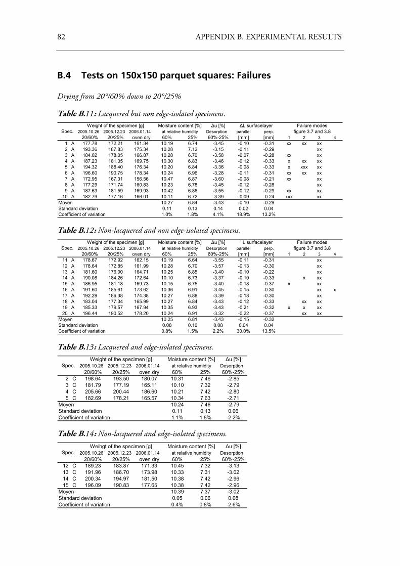
82 APPENDIX B. EXPERIMENTAL RESULTS
B.4 Tests on 150x150 parquet squares: Failures Drying from 20°/60% down to 20°/25%
Table B.11: Lacquered but non edge-isolated specimens. Δu [%]
2005.10.26 2005.12.23 2006.01.14 Desorption parallel perp.20/60% 20/25% oven dry 60% 25% 60%-25% [mm] [mm] 1 2 3 4
1 A 177.78 172.21 161.34 10.19 6.74 -3.45 -0.10 -0.31 xx xx xx2 A 193.36 187.83 175.34 10.28 7.12 -3.15 -0.11 -0.29 xx3 A 184.02 178.05 166.87 10.28 6.70 -3.58 -0.07 -0.28 xx xx4 A 187.23 181.35 169.75 10.30 6.83 -3.46 -0.12 -0.33 x xx xx5 A 194.32 188.40 176.34 10.20 6.84 -3.36 -0.08 -0.33 x xxx xx6 A 196.60 190.75 178.34 10.24 6.96 -3.28 -0.11 -0.31 xx xx xx7 A 172.95 167.31 156.56 10.47 6.87 -3.60 -0.08 -0.21 xx xx8 A 177.29 171.74 160.83 10.23 6.78 -3.45 -0.12 -0.28 xx9 A 187.63 181.59 169.93 10.42 6.86 -3.55 -0.12 -0.29 xx xx
10 A 182.79 177.16 166.01 10.11 6.72 -3.39 -0.09 -0.24 xxx xxMoyen 10.27 6.84 -3.43 -0.10 -0.29Standard deviation 0.11 0.13 0.14 0.02 0.04Coefficient of variation 1.0% 1.8% 4.1% 18.9% 13.2%
at relative humidityFailure modes
figure 3.7 and 3.8ΔL surfacelayerWeight of the specimen [g] Moisture content [%]
Spec.
Table B.12: Non-lacquered and non edge-isolated specimens. Δu [%]
2005.10.26 2005.12.23 2006.01.14 Desorption parallel perp.20/60% 20/25% oven dry 60% 25% 60%-25% [mm] [mm] 1 2 3 4
11 A 178.67 172.92 162.15 10.19 6.64 -3.55 -0.11 -0.31 xx12 A 178.64 172.85 161.99 10.28 6.70 -3.57 -0.13 -0.30 xx13 A 181.60 176.00 164.71 10.25 6.85 -3.40 -0.10 -0.22 xx14 A 190.08 184.26 172.64 10.10 6.73 -3.37 -0.10 -0.33 x xx15 A 186.95 181.18 169.73 10.15 6.75 -3.40 -0.18 -0.37 x xx16 A 191.60 185.61 173.62 10.36 6.91 -3.45 -0.15 -0.30 xx x17 A 192.29 186.38 174.38 10.27 6.88 -3.39 -0.18 -0.30 xx18 A 183.04 177.34 165.99 10.27 6.84 -3.43 -0.12 -0.33 xx xx19 A 185.33 179.57 167.94 10.35 6.93 -3.43 -0.21 -0.32 x x xx20 A 196.44 190.52 178.20 10.24 6.91 -3.32 -0.22 -0.37 xx xx
Moyen 10.25 6.81 -3.43 -0.15 -0.32Standard deviation 0.08 0.10 0.08 0.04 0.04Coefficient of variation 0.8% 1.5% 2.2% 30.0% 13.5%
Failure modesat relative humidity figure 3.7 and 3.8
° L surfacelayerMoisture content [%]Weight of the specimen [g]Spec.
Table B.13: Lacquered and edge-isolated specimens.
Δu [%]2005.10.26 2005.12.23 2006.01.14 Desorption
20/60% 20/25% oven dry 60% 25% 60%-25%2 C 198.64 193.50 180.07 10.31 7.46 -2.853 C 181.79 177.19 165.11 10.10 7.32 -2.794 C 205.66 200.44 186.60 10.21 7.42 -2.805 C 182.69 178.21 165.57 10.34 7.63 -2.71
Moyen 10.24 7.46 -2.79Standard deviation 0.11 0.13 0.06Coefficient of variation 1.1% 1.8% -2.2%
at relative humidityWeight of the specimen [g] Moisture content [%]
Spec.
Table B.14: Non-lacquered and edge-isolated specimens.
Δu [%]2005.10.26 2005.12.23 2006.01.14 Desorption
20/60% 20/25% oven dry 60% 25% 60%-25%12 C 189.23 183.87 171.33 10.45 7.32 -3.1313 C 191.96 186.70 173.98 10.33 7.31 -3.0214 C 200.34 194.97 181.50 10.38 7.42 -2.9615 C 196.09 190.83 177.65 10.38 7.42 -2.96
Moyen 10.39 7.37 -3.02Standard deviation 0.05 0.06 0.08Coefficient of variation 0.4% 0.8% -2.6%
at relative humidityWeihgt of the specimen [g] Moisture content [%]
Spec.
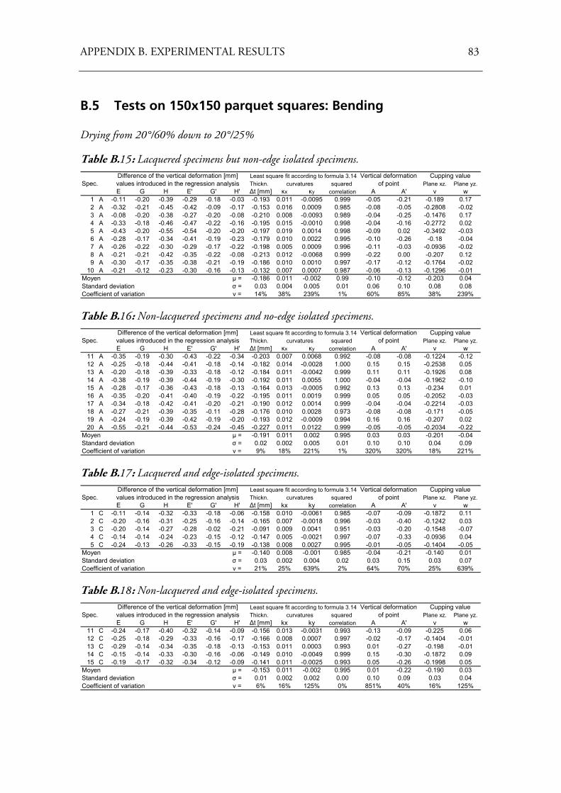
APPENDIX B. EXPERIMENTAL RESULTS 83
B.5 Tests on 150x150 parquet squares: Bending Drying from 20°/60% down to 20°/25%
Table B.15: Lacquered specimens but non-edge isolated specimens.
Spec. Thickn. squared Plane xz. Plane yz.E G H E' G' H' Δt [mm] κx κy correlation A A' v w
1 A -0.11 -0.20 -0.39 -0.29 -0.18 -0.03 -0.193 0.011 -0.0095 0.999 -0.05 -0.21 -0.189 0.172 A -0.32 -0.21 -0.45 -0.42 -0.09 -0.17 -0.153 0.016 0.0009 0.985 -0.08 -0.05 -0.2808 -0.023 A -0.08 -0.20 -0.38 -0.27 -0.20 -0.08 -0.210 0.008 -0.0093 0.989 -0.04 -0.25 -0.1476 0.174 A -0.33 -0.18 -0.46 -0.47 -0.22 -0.16 -0.195 0.015 -0.0010 0.998 -0.04 -0.16 -0.2772 0.025 A -0.43 -0.20 -0.55 -0.54 -0.20 -0.20 -0.197 0.019 0.0014 0.998 -0.09 0.02 -0.3492 -0.036 A -0.28 -0.17 -0.34 -0.41 -0.19 -0.23 -0.179 0.010 0.0022 0.995 -0.10 -0.26 -0.18 -0.047 A -0.26 -0.22 -0.30 -0.29 -0.17 -0.22 -0.198 0.005 0.0009 0.996 -0.11 -0.03 -0.0936 -0.028 A -0.21 -0.21 -0.42 -0.35 -0.22 -0.08 -0.213 0.012 -0.0068 0.999 -0.22 0.00 -0.207 0.129 A -0.30 -0.17 -0.35 -0.38 -0.21 -0.19 -0.186 0.010 0.0010 0.997 -0.17 -0.12 -0.1764 -0.02
10 A -0.21 -0.12 -0.23 -0.30 -0.16 -0.13 -0.132 0.007 0.0007 0.987 -0.06 -0.13 -0.1296 -0.01Moyen μ = -0.186 0.011 -0.002 0.99 -0.10 -0.12 -0.203 0.04Standard deviation σ = 0.03 0.004 0.005 0.01 0.06 0.10 0.08 0.08Coefficient of variation ν = 14% 38% 239% 1% 60% 85% 38% 239%
Cupping valueDifference of the vertical deformation [mm] values introduced in the regression analysis curvatures
Least square fit according to formula 3.14 Vertical deformation of point
Table B.16: Non-lacquered specimens and no-edge isolated specimens.
Spec. Thickn. squared Plane xz. Plane yz.E G H E' G' H' Δt [mm] κx κy correlation A A' v w
11 A -0.35 -0.19 -0.30 -0.43 -0.22 -0.34 -0.203 0.007 0.0068 0.992 -0.08 -0.08 -0.1224 -0.1212 A -0.25 -0.18 -0.44 -0.41 -0.18 -0.14 -0.182 0.014 -0.0028 1.000 0.15 0.15 -0.2538 0.0513 A -0.20 -0.18 -0.39 -0.33 -0.18 -0.12 -0.184 0.011 -0.0042 0.999 0.11 0.11 -0.1926 0.0814 A -0.38 -0.19 -0.39 -0.44 -0.19 -0.30 -0.192 0.011 0.0055 1.000 -0.04 -0.04 -0.1962 -0.1015 A -0.28 -0.17 -0.36 -0.43 -0.18 -0.13 -0.164 0.013 -0.0005 0.992 0.13 0.13 -0.234 0.0116 A -0.35 -0.20 -0.41 -0.40 -0.19 -0.22 -0.195 0.011 0.0019 0.999 0.05 0.05 -0.2052 -0.0317 A -0.34 -0.18 -0.42 -0.41 -0.20 -0.21 -0.190 0.012 0.0014 0.999 -0.04 -0.04 -0.2214 -0.0318 A -0.27 -0.21 -0.39 -0.35 -0.11 -0.28 -0.176 0.010 0.0028 0.973 -0.08 -0.08 -0.171 -0.0519 A -0.24 -0.19 -0.39 -0.42 -0.19 -0.20 -0.193 0.012 -0.0009 0.994 0.16 0.16 -0.207 0.0220 A -0.55 -0.21 -0.44 -0.53 -0.24 -0.45 -0.227 0.011 0.0122 0.999 -0.05 -0.05 -0.2034 -0.22
Moyen μ = -0.191 0.011 0.002 0.995 0.03 0.03 -0.201 -0.04Standard deviation σ = 0.02 0.002 0.005 0.01 0.10 0.10 0.04 0.09Coefficient of variation ν = 9% 18% 221% 1% 320% 320% 18% 221%
Difference of the vertical deformation [mm] values introduced in the regression analysis
Least square fit according to formula 3.14 Vertical deformation of point
Cupping valuecurvatures
Table B.17: Lacquered and edge-isolated specimens.
Spec. Thickn. squared Plane xz. Plane yz.E G H E' G' H' Δt [mm] kx ky correlation A A' v w
1 C -0.11 -0.14 -0.32 -0.33 -0.18 -0.06 -0.158 0.010 -0.0061 0.985 -0.07 -0.09 -0.1872 0.112 C -0.20 -0.16 -0.31 -0.25 -0.16 -0.14 -0.165 0.007 -0.0018 0.996 -0.03 -0.40 -0.1242 0.033 C -0.20 -0.14 -0.27 -0.28 -0.02 -0.21 -0.091 0.009 0.0041 0.951 -0.03 -0.20 -0.1548 -0.074 C -0.14 -0.14 -0.24 -0.23 -0.15 -0.12 -0.147 0.005 -0.0021 0.997 -0.07 -0.33 -0.0936 0.045 C -0.24 -0.13 -0.26 -0.33 -0.15 -0.19 -0.138 0.008 0.0027 0.995 -0.01 -0.05 -0.1404 -0.05
Moyen μ = -0.140 0.008 -0.001 0.985 -0.04 -0.21 -0.140 0.01Standard deviation σ = 0.03 0.002 0.004 0.02 0.03 0.15 0.03 0.07Coefficient of variation ν = 21% 25% 639% 2% 64% 70% 25% 639%
Difference of the vertical deformation [mm] values introduced in the regression analysis
Least square fit according to formula 3.14 Vertical deformation of point
Cupping valuecurvatures
Table B.18: Non-lacquered and edge-isolated specimens.
Spec. Thickn. squared Plane xz. Plane yz.E G H E' G' H' Δt [mm] kx ky correlation A A' v w
11 C -0.24 -0.17 -0.40 -0.32 -0.14 -0.09 -0.156 0.013 -0.0031 0.993 -0.13 -0.09 -0.225 0.0612 C -0.25 -0.18 -0.29 -0.33 -0.16 -0.17 -0.166 0.008 0.0007 0.997 -0.02 -0.17 -0.1404 -0.0113 C -0.29 -0.14 -0.34 -0.35 -0.18 -0.13 -0.153 0.011 0.0003 0.993 0.01 -0.27 -0.198 -0.0114 C -0.15 -0.14 -0.33 -0.30 -0.16 -0.06 -0.149 0.010 -0.0049 0.999 0.15 -0.30 -0.1872 0.0915 C -0.19 -0.17 -0.32 -0.34 -0.12 -0.09 -0.141 0.011 -0.0025 0.993 0.05 -0.26 -0.1998 0.05
Moyen μ = -0.153 0.011 -0.002 0.995 0.01 -0.22 -0.190 0.03Standard deviation σ = 0.01 0.002 0.002 0.00 0.10 0.09 0.03 0.04Coefficient of variation ν = 6% 16% 125% 0% 851% 40% 16% 125%
Vertical deformation of point
Cupping valuecurvatures
Difference of the vertical deformation [mm] values introduced in the regression analysis
Least square fit according to formula 3.14

84 APPENDIX B. EXPERIMENTAL RESULTS
Related Documents