Moist Adiabatic Lapse Rate in the Atmosphere and the Lifted ...

PhD – Environmental Fluid Mechanics – Physics of the AtmosphereUniversity of Trieste – International Center for Theoretical Physics

Moist Adiabatic Lapse Rate in the Atmosphereand the Lifted Parcel Theory (simplest version)

by Dario B. Giaiotti and Fulvio Stel (1)

Regional Meteorological Observatory, via Oberdan, 18/A I-33040 Visco (UD) – ITALY

AbstractThe dry adiabatic lapse rate is a useful conceptual and analytical model for the comprehension and forecast, but it fails on some layers of the Earth's atmosphere. For this reason new conceptual and analytic models have to be developed. What is here done, remaining in the realm of adiabatic processes (ascent or descent) is to derive the vertical thermal gradient for Earth's atmosphere when moisture and condensation is introduced into the lifted (shrunk) parcel. The results show a good agreement between observational data and the analytical model. In any case a right reproduction of the moist adiabatic lapse rate can be obtained only via numerical integration of the equation that describes the process.

The moist adiabatic lapse rateThe dry adiabatic lapse was obtained with the aid of the first principle of thermodynamics. The same should be done to derive the moista diabatic lapse rate. The conceptual model applied in solving this problem is that of the adiabatic ascent (descent) keeping into account the contribution coming from the water vapour into the ascending (descending) volume of air (i.e., parcel). Being adiabatic the entropy of the system must be conserved, then we can assume that

dSdz

=0

We can split the total system entropy into the three components coming from the water vapor, dry air and liquid water, then

dSdz

= ddz

M v svddz

M d sd ddz

M w sw =0

Being the process assumed as adiabatic, condensed water should remain inside the ascending (descending) parcel 1, moreover the total water mass M vM w=M water as well as the total dry air mass M d should be conserve, then

ddz

M v=−ddz

M w and ddz

M d=0

Substituting all these assumptions into the conservation of entropy we will have

1We will see later a process which is not strictly adiabatic because condensed water is withdrawn from the parcel during the ascent. This process is called “pseudo-adiabatic”.

dSdz

=svddz

M v M vddz

sv M dddz

sd swddz

M w M wddz

sw =0

then

dSdz

=svddz

M v M vddz

sv M dddz

sd−swddz

M vM wddz

sw=0

collecting the same vertical derivative of the vapour mass we obtaine

dSdz

= sv−swddz

M vM vddz

svM dddz

sdM wddz

sw =0

Remembering that the entropy difference is related to the latent heat of condensation (see previous

lectures) with the law sv−sw =l v

Twe obtain

dSdz

=l v

Tddz

M vM vddz

sv M dddz

sd M wddz

sw=0

Remembering the form of entropy for liquid water, dry air and water vapor (assuming the last two as ideal gases), we have respectively

dsw

dz=

cw

TdTdz

liquid water ,

dsd

dz=

c pd

TdTdz

−Rd

pd

dpd

dz dry air

and

dsv

dz=

c pv

TdTdz

−Rv

ededz

water vapour

Now we can simplify the above water vapour entropy vertical derivative assuming that the parcel has already reached saturation, then we can substitute the pressure e with the saturation vapour pressure es T , which depends only from temperature (for pure water), then we can write

dsv

dz=

c pv

TdTdz

−Rv

es

des

dTdTdz

This formula is in a much more "easy to use" form, in fact we have the tools to manage the vertical derivative of the saturation vapor pressure (Clausius-Clapeyron equation de s/dT ) and the vertical derivative of dry pressure (hydrostatic assumption dp /dz when pressure depends only from z). Substituting the entropy derivatives in the total entropy derivative we obtain

dSdz

=l v

Tddz

M vM v c pvM w cwM d c pd 1T

dTdz

−M v Rv

e s

des

dTdTdz

−M d Rd

pd

dpd

dz=0

at this point we introduce a new quantity, that is the total water mass (sum of liquid water and water vapour in the parcel) M=M wM v . We can use this new variable to substitute the mass of liquid water in the entropy vertical derivative, that is

dSdz

=l v

Tddz

M vM v c pvM−M vcwM d c pd 1T

dTdz

−M v Rv

es

des

dTdTdz

−M d Rd

pd

dpd

dz=0

then

dSdz

=l v

Tddz

M vM v c pv−cw M cvM d c pd 1T

dTdz

−M v Rv

es

des

dTdTdz

−M d Rd

pd

dpd

dz=0

Remembering that the temperature derivative of latent heat of condensation is equal to the differences in the specific heats at constant pressure and of liquid water (look at the lectures on the Clausius-Clapeyron)

dl v

dT=c pv−cw

we obtained

dSdz

=l v

Tddz

M vM v

dl v

dTM cvM d c pd

1T

dTdz

−M v Rv

es

des

dTdTdz

−M d Rd

pd

dpd

dz=0

Using now the approximated form of the Clausius-Clapeyron des

dT=e s l v /Rv T 2 to describe the

saturation pressure temperature derivative and rearranging the terms we obtain

dSdz

= ddz

l v

M v

TM cwM d c pd

1T

dTdz

−M d Rd

pd

dpd

dz=0

Dividing now all the terms for the dry air mass (remember that it is constant) we obtain

1M d

dSdz

= ddz l v M v

M d T M cwM d c pd M d

1T

dTdz

−Rd

pd

dpd

dz=0

Remembering that M v

M d=r is the mixing ratio and defining K≡

M cwM d c pd M d

we obtain

1M d

dSdz

= ddz l v r

T KT

dTdz

−Rd

pd

dpd

dz=0

Expliciting now the vertical derivative of the first term on the right we obtain

1M d

dSdz

= 1T

ddz l v r −

l v r T 2

dTdz

KT

dTdz

−Rd

pd

dpd

dz=0

Now two more assumptions are made: the first is based on the order of magnitude of the terms. In particular the second term on the right can be neglect because for the usual atmospheric conditions r~10−2 , moreover it is divided by T 2~7×104 K (a more precise approach can be adopted but it brings to the same result), then

1M d

dSdz

= 1T

ddz l v r K

TdTdz

−Rd

pd

dpd

dz=0

The second assumption is that of hydrostatic equilibrium2, then using the ideal gas law and confusing the dry pressure with the total pressure pd~ p≡pdes we obtain

1M d

dSdz

= 1T

ddz l v r K

TdTdz

gT=0

then

dTdz

=− gK− d

dz l v rK

This is the moist adiabatic lapse rate and its form is extremely similar to the dry adiabatic lapse rate

dTdz

dry=− g

c pd.

The first difference relies on the fact that K≡M cwM d c pd

M d≠c pd , nevertheless since the dry air

mass is greater than the total water mass of the parcel their difference is not as huge as one might think.

The second difference relies in the extra term on the right, that is essentially the vertical derivative of the product of latent heat of condensation and mixing ratio, which takes into account the amount of heat released by the water vapor when it condenses. Since mixing ratio decreases because of condensation, the derivative is negative, then the lapse rate is higher (i.e., temperature decreases less than in the case of dry ascent) when condensation takes place. With further assumptions it is possible to give an order of magnitude for the moist adiabatic lapse rate, in particular assuming that the latent heat of condensation is constant with temperature (see lectures on Clausius-Clapeyron) we obtain

dTdz

~− gK−

l v

Kdrdz

=− gK 1 l v

gdrdz

Because of the condensation during ascent, mixing ratio decreases with altitude, then the moist adiabatic lapse rate should be lower (in absolute value) than the dry adiabatic one, in other words 2 The hydrostatic approximation can become a too crude approximation, specially dealing with strong vertical

accelerations that characterize thunderstorms. In these cases, as we will see, the hydrostatic approximation should be overcome.

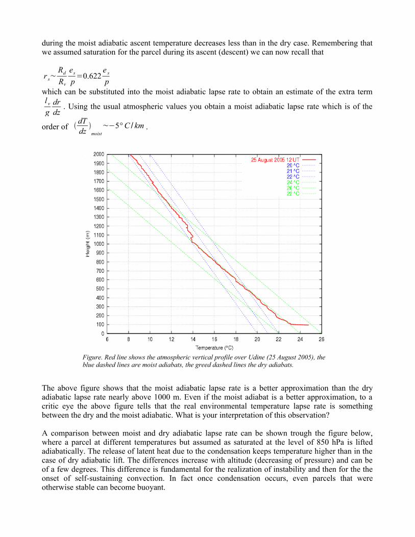
during the moist adiabatic ascent temperature decreases less than in the dry case. Remembering that we assumed saturation for the parcel during its ascent (descent) we can now recall that

r s~Rd

Rv

es

p=0.622

e s

pwhich can be substituted into the moist adiabatic lapse rate to obtain an estimate of the extra term l v

gdrdz

. Using the usual atmospheric values you obtain a moist adiabatic lapse rate which is of the

order of dTdz

moist

~−5° C / km .

The above figure shows that the moist adiabatic lapse rate is a better approximation than the dry adiabatic lapse rate nearly above 1000 m. Even if the moist adiabat is a better approximation, to a critic eye the above figure tells that the real environmental temperature lapse rate is something between the dry and the moist adiabatic. What is your interpretation of this observation?

A comparison between moist and dry adiabatic lapse rate can be shown trough the figure below, where a parcel at different temperatures but assumed as saturated at the level of 850 hPa is lifted adiabatically. The release of latent heat due to the condensation keeps temperature higher than in the case of dry adiabatic lift. The differences increase with altitude (decreasing of pressure) and can be of a few degrees. This difference is fundamental for the realization of instability and then for the the onset of self-sustaining convection. In fact once condensation occurs, even parcels that were otherwise stable can become buoyant.

F

Figure. Red line shows the atmospheric vertical profile over Udine (25 August 2005), the blue dashed lines are moist adiabats, the greed dashed lines the dry adiabats.

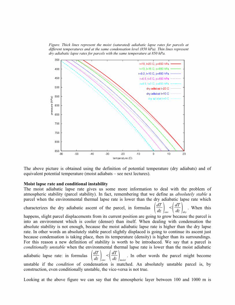
The above picture is obtained using the definition of potential temperature (dry adiabats) and of equivalent potential temperature (moist adiabats – see next lectures).

Moist lapse rate and conditional instabilityThe moist adiabatic lapse rate gives us some more information to deal with the problem of atmospheric stability (parcel stability). In fact, remembering that we define as absolutely stable a parcel when the environmental thermal lapse rate is lower than the dry adiabatic lapse rate which

characterizes the dry adiabatic ascent of the parcel, in formulas dTdz env

dTdz dry

. When this

happens, slight parcel displacements from its current position are going to grow because the parcel is into an environment which is cooler (denser) than itself. When dealing with condensation the absolute stability is not enough, because the moist adiabatic lapse rate is higher than the dry lapse rate. In other words an absolutely stable parcel slightly displaced is going to continue its ascent just because condensation is taking place, then its temperature (density) is higher than its surroundings. For this reason a new definition of stability is worth to be introduced. We say that a parcel is conditionally unstable when the environmental thermal lapse rate is lower than the moist adiabatic

adiabatic lapse rate: in formulas dTdz env

dTdz moist

. In other words the parcel might become

unstable if the condition of condensation is matched. An absolutely unstable parcel is, by construction, even conditionally unstable, the vice-versa is not true.

Looking at the above figure we can say that the atmospheric layer between 100 and 1000 m is

Figure. Thick lines represent the moist (saturated) adiabatic lapse rates for parcels at different temperatures and at the same condensation level (850 hPa). Thin lines represent dry adiabatic lapse rates for parcels with the same temperature at 850 hPa.

composed by parcels which are almost absolutely neutral (the environmental lapse rate is nearly dry adiabatic) but which are even conditionally unstable (the environmental lapse rate is lower than the moist adiabatic one). With a slight abuse of language then we say that the layer between 100 and 1000 m is conditionally unstable. Conditional instability explains why, even in absolutely stable layers, some small cumulus can develop. This happens because, by chance, some portions of air are moister than others, then these parcels can reach saturation, then they can buoy.

Buoyancy and the “lifted parcel theory” (simple version)The importance of vertical thermal gradients arises directly from the equation of motion, in particular from the inviscid and non rotating form. For simplicity we will consider just the vertical component of such equation, that is

ρ dwdt

=−∂ p∂ z

−gρ

If we subtract to this equation a reference state characterized by hydrostatic equilibrium

0=−∂ p0

∂ z−gρ0

we obtain

ρ dwdt

=− ∂∂ z

p−p0−g ρ− ρ0

then

dwdt

=−1ρ

∂∂ z

p− p0−g ρ− ρ0

ρ

The first term on the right is called vertical perturbation gradient force and it depends, apart from density, from a gradient in vertical pressure perturbations p− p0 then both from non hydrostatic effects on pressure and from density anomalies, that can be even hydrostatic. The second term is called buoyancy force

B=−g ρ−ρ0

ρ

and it depends only from density perturbations. The buoyancy term written in this way is not in a useful form because of the presence of perturbed density, for this reason the reference state of density is usually taken. Moreover the ideal gas law is introduced to substitute density with pressure and temperature, then we obtain

B≃−g ρ−ρ0

ρ0=−g

RTp−

RT 0

p0 RT 0

p0

with some algebra this become

B≃−g1− TT 0

p0

p Since for standard atmospheric conditions the perturbed pressure differs by a fee percent from its reference status usually we can write

B~−g1− TT 0 =−gT 0−T

T 0 .

With this approximation of buoyancy force we can rewrite the vertical component of the inviscid, non-rotating Navier-Stokes equation, that is

dwdt

≃− 1ρ0

∂∂ z

p− p0−gT 0−T

T 0

Neglecting the pressure perturbation vertical gradient the above equation becomes

dwdt

~−gT 0−T

T 0

which is the usual form adopted to describe the lifted parcel theory, in fact it represents the lagrangian acceleration acting on a parcel because of its temperature differences with a reference state, assumed as the environment. The neglecting of the vertical gradient of pressure perturbations p− p0 (sometimes called aerodynamic drag) is fundamental for the applicability of the parcel theory and then it is worth to spend a few more words on it, at least qualitatively. In fact the vertical acceleration due to the buoyancy depends only form the difference in temperatures (reference state and parcel.) while the dynamic acceleration (downward directed for an upward movement) depends even from the lateral magnitude of the parcel. In other words large parcels experience huger downward accelerations than smaller ones even with the same temperature difference with the environment. For this reason parcel theory is a good approximation for reality when dealing with small parcels (but not too small, try to explain why), as usually happens at middle latitudes, but not as well dealing with large ones as usually happens at the tropics.

Convective available potential energy (CAPE) and convective inhibition (CIN)

The vertical integral of buoyancy is called CAPE, which stands for Convective Available Potential Energy. The origin of this name, as well as its physical interpretation springs from its analytical approach, in particular starting from the lifted parcel equation we have

dwdt

w=−gT 0−T

T 0w

then

12

dw2

dt=−g

T 0−T T 0

dzdt

integrating it from the point where the lifted parcel starts to be buoyant (level of free convection, LFC) up to the point where the parcel is no more buoyant we obtain

12∫LFC

ELdw2=−g∫LFC

EL T 0−T T 0

dz

Assuming that the vertical velocity at the lifting condensation level is null (w(LFC)=0), we obtain

w2EL=−2g∫LFC

EL T 0−T T 0

dz=2CAPE

This result, even if too crude as we will see, is nevertheless extremely important because it relates the vertical velocity, a parameter directly related to the severity of atmospheric convection, to the thermodynamic vertical stratification. For this reason CAPE was in the past widely used. Nowadays CAPE is no more considered as important as in the past for several reasons.The first reason is that the above maximum vertical velocity is by far a too large upper estimate of the real one. In fact the lifted parcel theory does not take into account the aerodynamic drag as well as the hydrometeor loading which in deep moist convection can become dominant. The second reason is that sometimes CAPE is not uniquely determined, as can happen in cases of inversions,that is when the atmospheric stratification hosts layers where parcels are no more buoyant embedded in layers where the parcel is buoyant. Moreover the choice of the starting parcel is pivotal for the definition of CAPE. The third reason is that even small CAPE values can give rise to relatively high values of vertical velocities (100 J/kg correspond to nearly 15 m/s) and it does not give any information concerning the possibility of the effective CAPE release. In other words CAPE gives information just concerning the fuel available for deep moist convection and not concerning its onset, which is currently considered as one of the major research topics in atmospheric sciences.Before to conclude the discussion on CAPE it is worth to spend a few more words concerning the integral of buoyancy from the ground (assumed as the starting point of the parcel) up to the level of free convection, in other words

12∫GRD

LFCdw2=−g∫GRD

LFC T 0−T T 0

dz=CIN

This quantity is called convective inhibition and it represents the amount of kinetic energy that you should give to the parcel to reach its level of free convection, then the level at which CAPE start to be released. CIN represents the inhibition to convection (then its name) and represents as well a lower threshold for the strength of the forcing mechanism for convection. CIN, as well as CAPE, are always referred to a specific parcel, then different parcels can have (and usually it is so) different CAPEs and CINs.

Equivalent potential temperature and saturated equivalent potential temperatures

Potential temperature was derived as a generalization of the concept of dry adiabatic lapse rate. Equivalent potential temperature is a conserved quantity for dry adiabatic ascents (descents) and it is related to the entropy conservation. Introducing moisture and condensation potential temperature is no more conserved but you can guess that a similar quantity can be derived with similar properties (conserved during an adiabatic ascent). To determine this quantity we start from the moist lapse rate equation, that is

ddtl v rv

Tr t c

w−c pd 1

TdTdt

−Rd

pdpdt

=0

At this point using the differentiation rules and defining the constant c pt =r t c

w−c pd

, the above equation can be written in the more compact form

ddtl v rv

Tc p

t ddtln T −Rd

ddt

ln p=0

that builds a relationship between temperature and pressure in the case of an adiabatic, reversible and saturated process. Now we have to remember that our aim is that of obtaining a potential temperature, that is a temperature independent from the pressure. To describe this process we should eliminate the explicit dependence from pressure in the first therm. This can be done defining the following potential temperature

Θ=T p0

p Rd

c pt

This potential temperature is not exactly the potential temperature for dry air, because c pv ≠c p

d and

c pt ≠r v c p

v c pd=c p , but these two potential temperatures slightly differ because in the usual

meteorological conditions r t≪1 and c pt ≃r v c p

v c pd≃c p

d.

Taking the logarithm and differentiating the above potential temperature we will have

ddt ln Θ = d

dtln T −

Rd

c pt

ddt

ln p

that can be used to substitute the pressure and temperature terms in the entropy conservation equation, that is

ddtl v rv

Tc p

t ddtln Θ =0

This equation can be easily solved integrating from the initial state characterized by r vi , T and Θ to the final state characterized by r v f=0 , T f and Θ f . After the integration we obtain

c pt ln

Θ f

Θ i

l v r v f

T f−

l v r vi

T i=0

then

c pt ln

Θ f

Θ i=

l v r vi

T i

The quantity Θ f is the final value of the potential temperature once the air parcel had been brought up to an altitude where all its water vapor is condensed, keeping the result of condensation (liquid water) into the air parcel during the ascent. This quantity, for the above reasons, is called equivalent potential temperature and has the form

Θe=Θ exp c pt

l v r v

T

where T , r v and Θ are, respectively, the current parcel temperature, vapor mixing ratio and potential temperature (but pay attention that this is just an approximation as told above). This form of the equivalent potential temperature is not the most general, because, as you probably remember, it was determined assuming that the initial parcel was saturated, i.e., its vapor pressure was that of saturation for its temperature. A more general form, useful even for unsaturated parcels, can be obtained assuming that the unsaturated parcel is lifted adiabatically up to the level at which condensation occurs (usually called Lifting Condensation Level – LCL). Then, when condensation occurs and the parcel becomes saturated, we can obtain its equivalent potential temperature using the already obtained equation for saturated processes. In other words the equivalent potential temperature of an unsaturated parcel is the equivalent potential temperature obtained starting from its lifting condensation level (LCL) which, in turn, is function of the current parcel pressure, temperature and vapor mixing ratio. In its compact form the equivalent potential temperature for an unsaturated parcel becomes

Θe=ΘLCL p ,T , rv ⋅expc pt

l v r v

T LCL

The determination of the lifting condensation potential temperature ΘLCL is not a real problem, in fact because during the adiabatic ascent the potential temperature Θ is conserved, we can say that Θ≡ΘLCL . The only problem, approximations apart, is the determination of T LCL , that is the temperature at the LCL. This can be done using the Γ dew and Γ dry vertical lapse rates or recursively (more precise). Just taking the analytical approach we can write T dew z =Γ dew⋅zT dew 0 and T dry z =Γ dry⋅zT dry 0 , because at the LCL temperature and dew point temperature must coincide, we should have T dry z ≡T dew z then

zlcl=T dry0−T dew0

Γ dew−Γ dry

inserting the so far obtained z lcl in one of the equations that describe the vertical temperature trends, we will have

T lcl=Γ dry⋅T dry 0−T dew 0

Γ dew−Γ dryT dry 0

which gives us the temperature at the lifting condensation level once are known the dew point and thermal vertical lapse rates as well as the current temperature of the parcel. This T lcl can be used in the equivalent potential temperature equation

Θe=Θ⋅expc pt

l v rv

T LCL .

Equivalent potential temperature is, by construction, conserved during moist and dry adiabatic ascents and it plays the same role of potential temperature for dry air when condensation occurs. In other words the criteria for conditional instability is that the equivalent potential temperature is lower than zero provided that the parcel is saturated, in other words

∂Θ e

∂ z saturated0

means that a parcel is unstable in the layer characterized by the above negative equivalent potential temperature lapse rate. But what happens if we are not in a saturated layer? In that case another quantity is used, that is the saturated equivalent potential temperature Θes , defined as the equivalent potential temperature is the parcel (layer) is assumed saturated at its temperature. Saturated equivalent potential temperature is simply derived by the following formula

Θes=Θ⋅expc pt

lv r s

T

where r s is the saturated mixing ratio at the parcel temperature T. Using the saturated equivalent potential temperature a general criteria for the conditional instability, valid both for saturated and unsaturated parcels, is

∂Θes

∂ z0

Equivalent potential temperature and convective (potential) instabilityAll the so far discussed instabilities (absolute and conditional) are referred to a parcel and only with a slight abuse, since layers are defined as portions of atmosphere with the same thermal lapse rate, these instabilities are referred to a whole layer. In atmospheric physics, however, there is another kind of instability which is, by construction, referred to a whole layer and not to a parcel. This instability is called convective instability or, equivalently, potential instability. A layer is defined as convectively (potentially) unstable when if lifted its bottom reaches saturation before than is top, then during the further adiabatic ascent the layer bottom cools slowly than the layer top and the layer is then conditionally unstable. Conditionally unstable layers are, by construction, even convectively unstable but even absolutely stable layers can become conditionally unstable when the equivalent potential temperature lapse rate is negative, then the condition for convective (potential) instability is

∂Θe

∂ z0 .

This can be easily understood remembering that equivalent potential temperature is conserved during the adiabatic ascents, then if the layer, at a certain time t during its displacement becomes conditionally unstable (e.g., shows negative saturated equivalent potential temperature lapse rate) this means that at time t 0 (at the beginning of its displacement) its equivalent potential temperature (which is conserved during the ascent, then equal to the saturated equivalent potential temperature at

time t) should show a similar behavior, then a negative lapse rate.

The hidden concept of convective instability is that of layer displacement. Even hidden, this concept is extremely important and sustain all the convective (potential) instability idea. Without such a displacement, conditional instability will not take place even if the equivalent potential temperature has a negative lapse rate. Then even if a proper forcing is going to occur for the realization of conditional instability no free buoyancy is going to be reached.

Usually the concept of potential (convective) instability is found to be extremely useful as a forecasting criteria on the plains in the neighborhood of mountain ridges. In these cases the layer displacement, as well as the forcing for the realization of the conditional instability, is represented by the orographic lifting. Other situations where the determination of convective instability is found to be useful for the forecasting of the onset of deep moist convection is represented by fronts (large scale dynamic lifting).

The adiabatic liquid water content

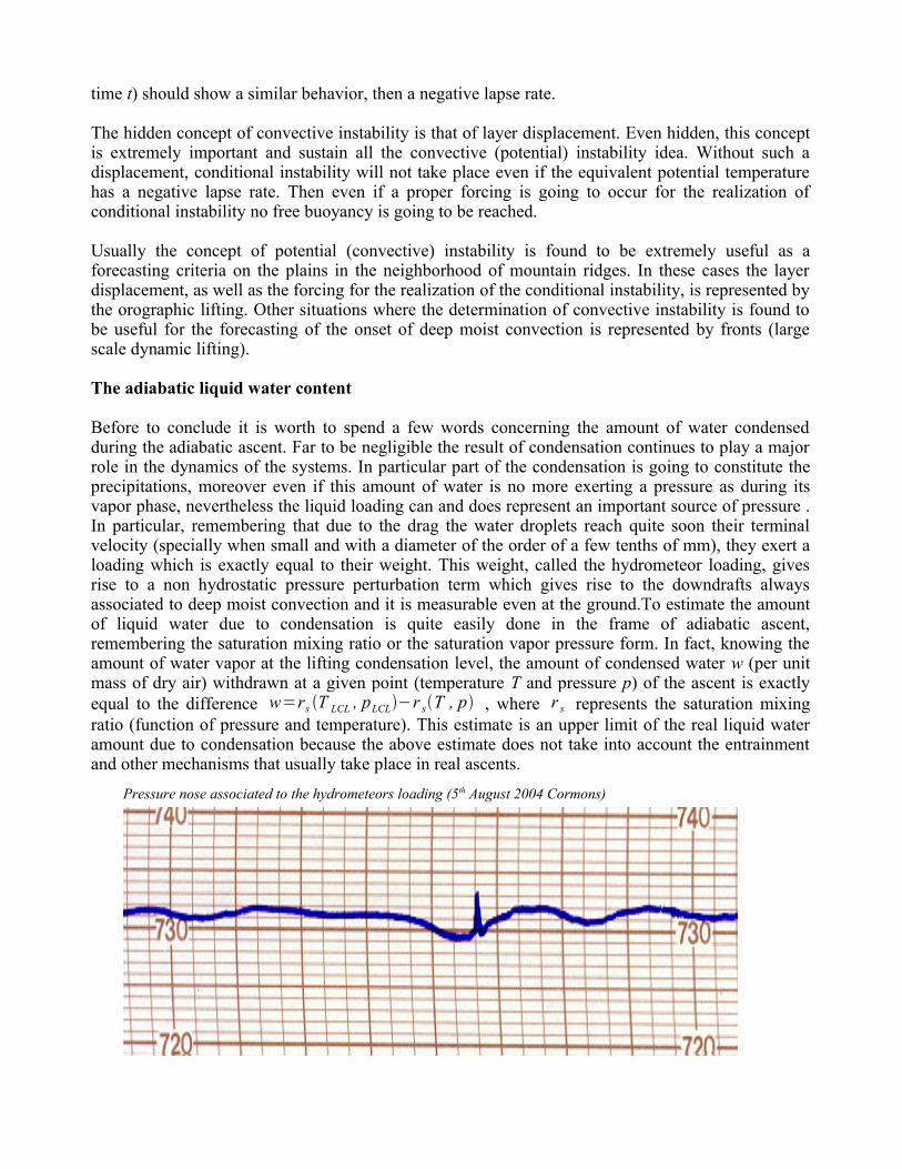
Before to conclude it is worth to spend a few words concerning the amount of water condensed during the adiabatic ascent. Far to be negligible the result of condensation continues to play a major role in the dynamics of the systems. In particular part of the condensation is going to constitute the precipitations, moreover even if this amount of water is no more exerting a pressure as during its vapor phase, nevertheless the liquid loading can and does represent an important source of pressure . In particular, remembering that due to the drag the water droplets reach quite soon their terminal velocity (specially when small and with a diameter of the order of a few tenths of mm), they exert a loading which is exactly equal to their weight. This weight, called the hydrometeor loading, gives rise to a non hydrostatic pressure perturbation term which gives rise to the downdrafts always associated to deep moist convection and it is measurable even at the ground.To estimate the amount of liquid water due to condensation is quite easily done in the frame of adiabatic ascent, remembering the saturation mixing ratio or the saturation vapor pressure form. In fact, knowing the amount of water vapor at the lifting condensation level, the amount of condensed water w (per unit mass of dry air) withdrawn at a given point (temperature T and pressure p) of the ascent is exactly equal to the difference w=rs T LCL , pLCL−r sT , p , where r s represents the saturation mixing ratio (function of pressure and temperature). This estimate is an upper limit of the real liquid water amount due to condensation because the above estimate does not take into account the entrainment and other mechanisms that usually take place in real ascents.

Pressure nose associated to the hydrometeors loading (5th August 2004 Cormons)

Pseudo equivalent potential temperature

Before to conclude a few words concerning pseudo equivalent potential temperature are needed. The equivalent potential temperature has been obtained by the following differential equation

ddtl v rv

Tr t c

w−c pd 1

TdTdt

−Rd

pdpdt

=0

where r t is the total water mixing ratio (liquid plus vapor) which is considered constant during the ascent. But we can imagine that liquid water is removed after condensation, then the total mixing ratio is no more constant and, if we assume that all the condensed water is removed, we have to substitute r t with r sT , p , the saturation mixing ratio for vapor only, which is function of temperature and pressure. The above equation becomes

ddtl v rv

Tr sT , pcw−c p

d 1T

dTdt

−Rd

pdpdt

=0

which can be solved only numerically. However some naive considerations can be done on the potential temperature which is conserved in this kind of pseudo-adiabatic ascent (no more adiabatic, in fact a part of the water is lost) and is called pseudo-equivalent potential temperature. Looking at the form of equivalent potential temperature

Θe=Θ⋅expc pt

l v rv

T LCL

we have to remember that c pt =r t c

w−c pd , then being r t c

w−c pdr s cw−c p

d and being this inequality growing with the ascent (more and more water vapor is lost as the parcel is lifted), the exponential in the pseudo-equivalent potential temperature should be smaller than in the case of its equivalent potential case, then pseudo-equivalent potential temperature is smaller than the equivalent potential one and their difference is higher for larger displacements. In other words in a pseudo-adiabatic ascent a parcel becomes cooler than in an adiabatic ascent as it is obvious, loosing matter (then heat).

All done for the equivalent potential temperature can be done as well for the pseudo-equivalent one. Usually, dealing with deep-moist convection, pseudo-equivalent potential temperature is found to be more useful since precipitation does occur in deep moist convection, then we need a variable which can be able to comprehend the formation of precipitations.