Module I 1. Open loop control system & Closed loop control ...

Module I

1. Open loop control system & Closed loop control system

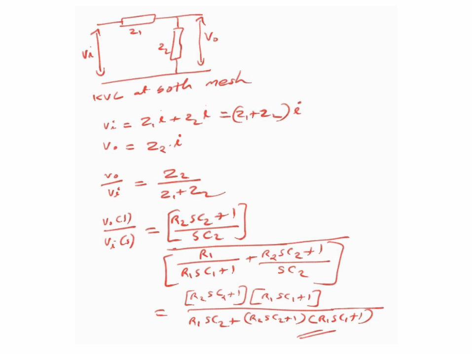
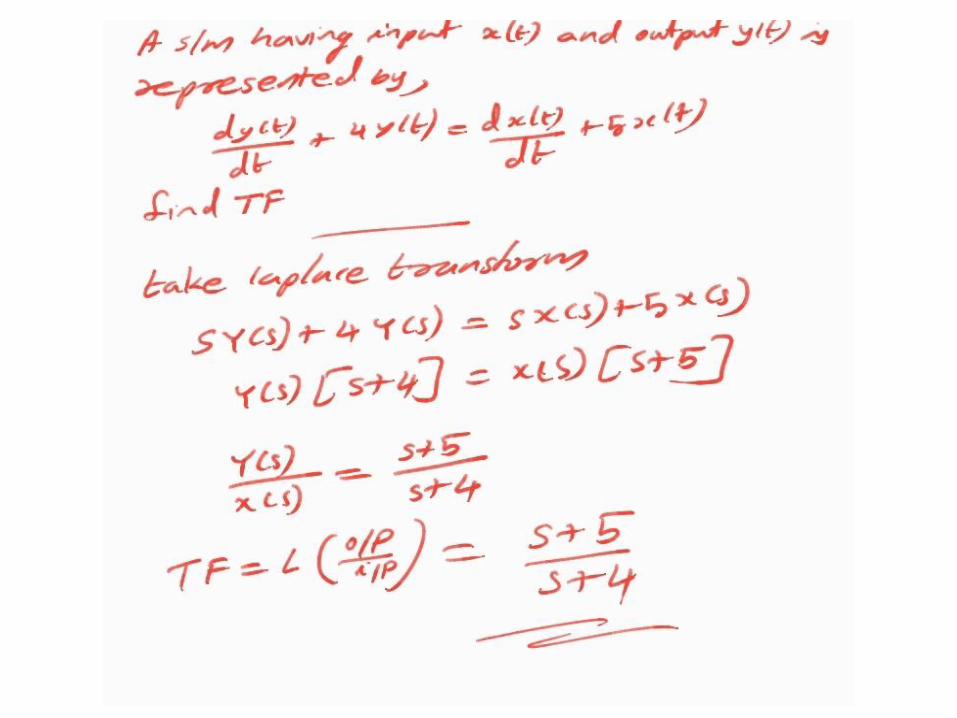
2. Transfer function of LTI systems

3. Mechanical and Electromechanical Systems

4. Force Voltage and Force Current analogy

5. Block diagram representation

6. Block diagram reduction

7. Signal flow graph

8. Mason's gain formula

9. Characteristics equation

SYSTEM

System when a number of elements or components are connected

in a sequence to perform a specific function, the group thus

formed is called a system.

Example: a lamp (made up of glass, filaments)

CONTROL SYSTEM

In a system when the output quantity is controlled by varying the

input quantity the system is called control system

Example: a lamp controlled by a switch

The output quantity is called controlled variable or response

The input quantity is called command signal or excitation

open loop control system

&

closed loop control system

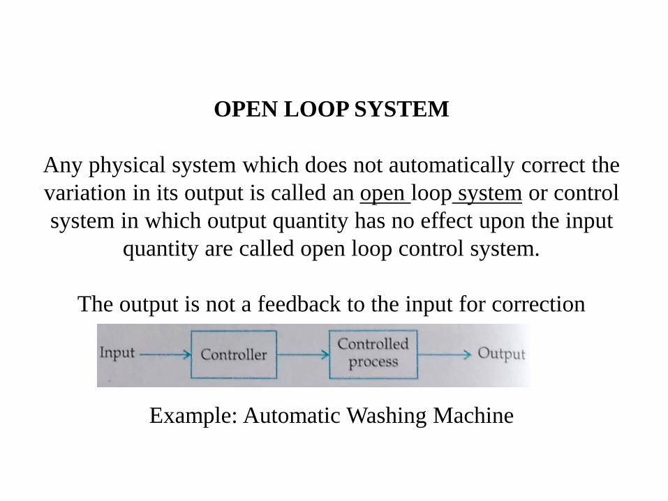
OPEN LOOP SYSTEM

Any physical system which does not automatically correct the

variation in its output is called an open loop system or control

system in which output quantity has no effect upon the input

quantity are called open loop control system.

The output is not a feedback to the input for correction

Example: Automatic Washing Machine

OPEN LOOP SYSTEM

Advantage

1. simple

2. economical

3. easier to construct

4. stable

Disadvantage

1. inaccurate

2. unreliable

3. the changes in the output due to external disturbances are not

corrected automatically

CLOSED LOOP SYSTEM

(automatic control system)

control systems in which the output has an effect upon the input

quantity in order to maintain the desired output value are called

closed loop control systems

Example: Air conditioner provided with thermostat

CLOSED LOOP SYSTEM

Advantage

1. accurate

2. the sensitivity of the system may be made small to make the

3. system more stable

4. less affected by noise

Disadvantage

1. complex

2. costly

3. feedback in closed loop system may lead to oscillatory

4. response feedback reduces the overall gain of the system

5. stability is a major problem in closed loop system

Open loop system

these are not reliable

it is easier to build

if calibration is good

they perform accurately

operating systems are

generally more stable

Optimization is not

possible

Closed loop system

these are reliable

it is difficult to built

they are accurate

because of feedback

these are less stable

Optimization is possible

Comparison between open loop system and closed

loop system

MATHEMATICAL MODEL OF CONTROL SYSTEM

Control system is a collection of physical object connected

together to serve an objective

The input output relations of various physical components of a

system are governed by differential equation

The mathematical model of a control system constitutes a set of

differential equations

The response or output of the system can be studied by solving

the differential equations for various input condition

MATHEMATICAL MODEL OF CONTROL SYSTEM

The differential equations of a linear time invariant system can be

reshaped into different form for the convenience of analysis

One such model for single input and single output system

analysis is called transfer function

TRANSFER FUNCTION

Transfer function is the ratio of Laplace transform of outputs of the

system to the Laplace transform of the inputs under the assumption

that all initial conditions are zero

TRANSFER FUNCTION

Transfer function is the ratio of Laplace transform of outputs of the

system to the Laplace transform of the inputs under the assumption

that all initial conditions are zero

Advantages of Transfer function

1. The response of the system to any input can be determined very

easily.

2. It gives the gain of the system.

3. It help in the study of stability of the system

4. Since Laplace transform is used it converts time domain

equations to simple algebraic equations

5. Poles and zeroes of a system can be determined from the

knowledge of the transfer function of the system.

Disadvantages

1. transfer function cannot be defined for Non linear system

2. transfer function is defined only for linear system

3. from the transfer function physical structure of a system cannot

determine

4. initial conditions lose their importance

Characteristic Equation (C.E)

The characteristic equation of a linear system can be obtained by

equating the denominator polynomial of the transfer function to

zero. The roots of the characteristic equation are the poles of

corresponding transfer function.

Poles of a transfer function

The value of ‘S’ which makes the transfer function infinite after

substitution in the denominator of a transfer function are called

poles of that transfer function

Zeros of a transfer function

The value of ‘S’ which make the transfer function zero after

substituting in the numerator are called zeros of that transfer

function

)R(s)bs.....bsbsb)C(s)asa......sas(a

transformLaplace thetake

constants are b'' and a'' where

r(t)bdt

dr(t)........b

dt

r(t)db

dt

r(t)dbc(t)a

dt

dc(t)a..........

dt

c(t)da

dt

c(t)da

equation aldifferentiorder n following by the described becan relation output -input The

system theofoutput theisc(t)t &r(t)input having systemlinear aConsider

01

1-m

1-m

m

m01

1-n

1-n

n

n

011-m

1-m

1mm

m

m011-n

1-n

1-nn

n

n

th

01

1-n

1-n

n

n

01

1-m

1-m

m

m

asa......sasa

bs.....bsbsb

R(s)

C(s)TF

0f)es)(dsS.(S).........S)(SS(S:C.E

2d

dfee- ,,......SS,S:Poles

2a

acbb- ,,......SS,S:Zeros

f)es)(dsS.(S).........S)(SS(S

c)bs)(asS.(S).........S)(SSK(S

R(S)

C(S)TF

2

n21

2

n21

2

mba

2

n21

2

mba

Basic formula

L[x(t)]=X(S)

L[I(t)]=I(S)

condition initial zerowith X(S)S]dt

x(t)dL[

condition initial zerowith SX(S)]dt

dx(t)L[

22

Mechanical system

two types

1. translational systems

2. rotational systems

The motion takes place along a straight line is known as

translational motion.

The rotational motion of a body can be defined as the motion of a

body about a fixed axis.

Mechanical translational system

The model of mechanical translational system can be obtained by

using three basic elements mass, spring and dashpot.

The weight of the mechanical system is represented by the element of

mass

The elastic deformation of the body can be represented by spring

The friction existing in rotating mechanical system can be represented

by dashpot

When a force is applied to a translational mechanical system it is

opposed by opposing forces due to mass, friction and elasticity of the

system

Force acting on a mechanical body are governed by Newton's second

law of motion

Guidelines to determine the transfer function of mechanical

translational system

1. consider each mass separately

2. draw the free body diagram

3. write the differential equations

4. take the Laplace transform of differential equations

5. rearrange the s-domain equation to eliminate the unwanted

variables and obtain the ratio between output variable and input

variable

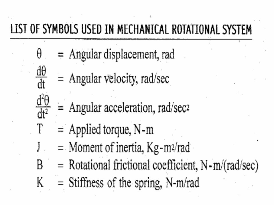
Mechanical rotational systems

The model of mechanical rotational systems can be obtained by

using three elements moment of inertia [J] of mass, dash-pot with

rotational frictional Coefficient [B] and torsional spring with

stiffness [K]

The weight of the rotational mechanical system is represented by

the moment of inertia of the mass

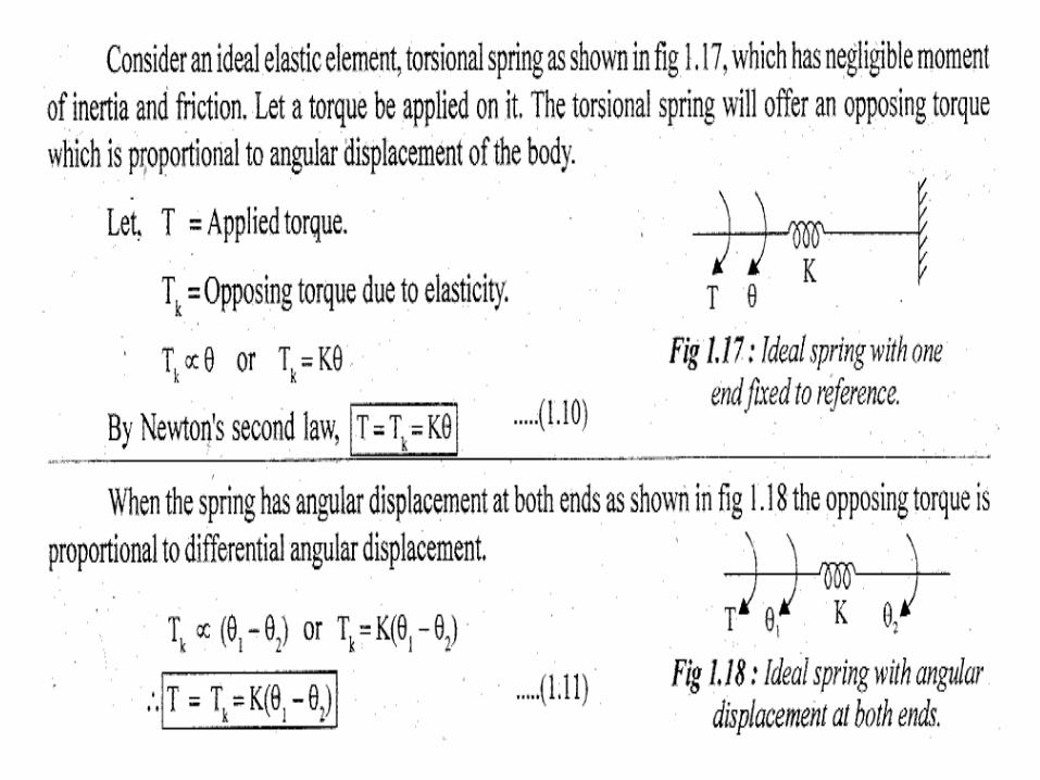
The elastic deformation of the body can be represented by a

spring

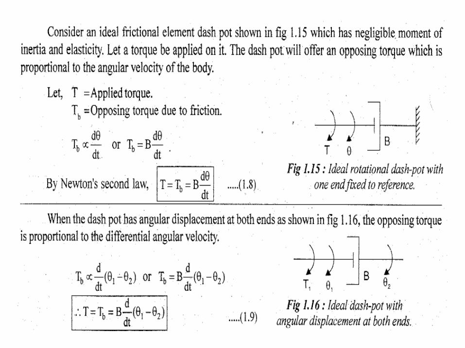
The friction existing in rotational mechanical system can be

represented by dash-pot

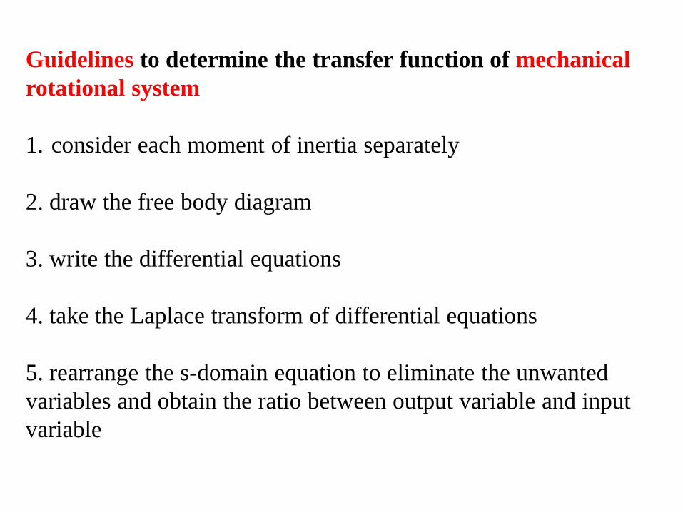
Guidelines to determine the transfer function of mechanical

rotational system

1. consider each moment of inertia separately

2. draw the free body diagram

3. write the differential equations

4. take the Laplace transform of differential equations

5. rearrange the s-domain equation to eliminate the unwanted

variables and obtain the ratio between output variable and input

variable

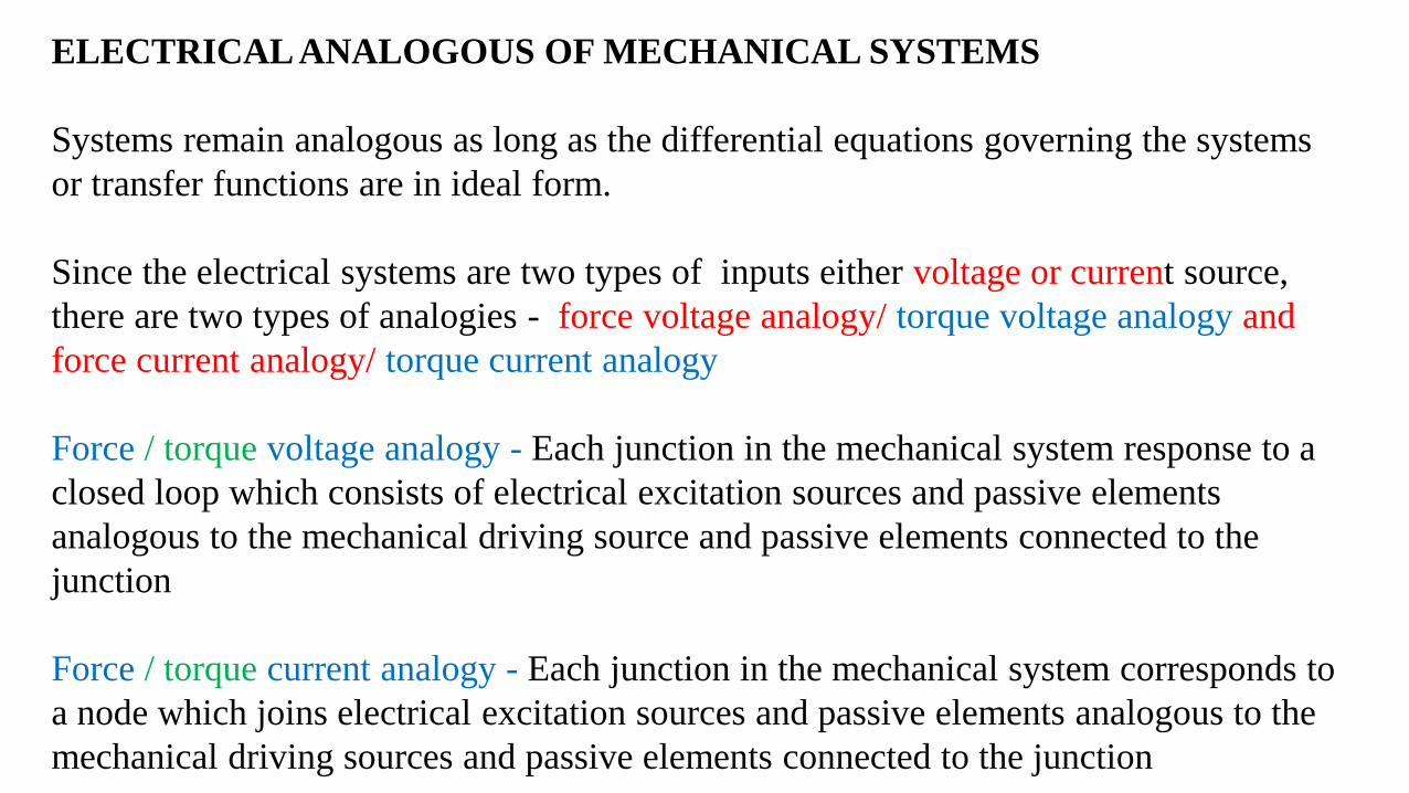
ELECTRICAL ANALOGOUS OF MECHANICAL SYSTEMS

Systems remain analogous as long as the differential equations governing the systems

or transfer functions are in ideal form.

Since the electrical systems are two types of inputs either voltage or current source,

there are two types of analogies - force voltage analogy/ torque voltage analogy and

force current analogy/ torque current analogy

Force / torque voltage analogy - Each junction in the mechanical system response to a

closed loop which consists of electrical excitation sources and passive elements

analogous to the mechanical driving source and passive elements connected to the

junction

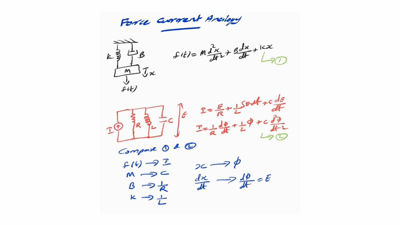
Force / torque current analogy - Each junction in the mechanical system corresponds to

a node which joins electrical excitation sources and passive elements analogous to the

mechanical driving sources and passive elements connected to the junction

BLOCK DIAGRAM

A block diagram of a system is a pictorial representation of the functions performed by

each component and of the flow of signals.

The elements of a block diagram are block, branch point and summing point.

Block - is a symbol for the mathematical operation on the input signal to the block that

produces the output

The transfer function of the components are usually ended in the corresponding blocks.

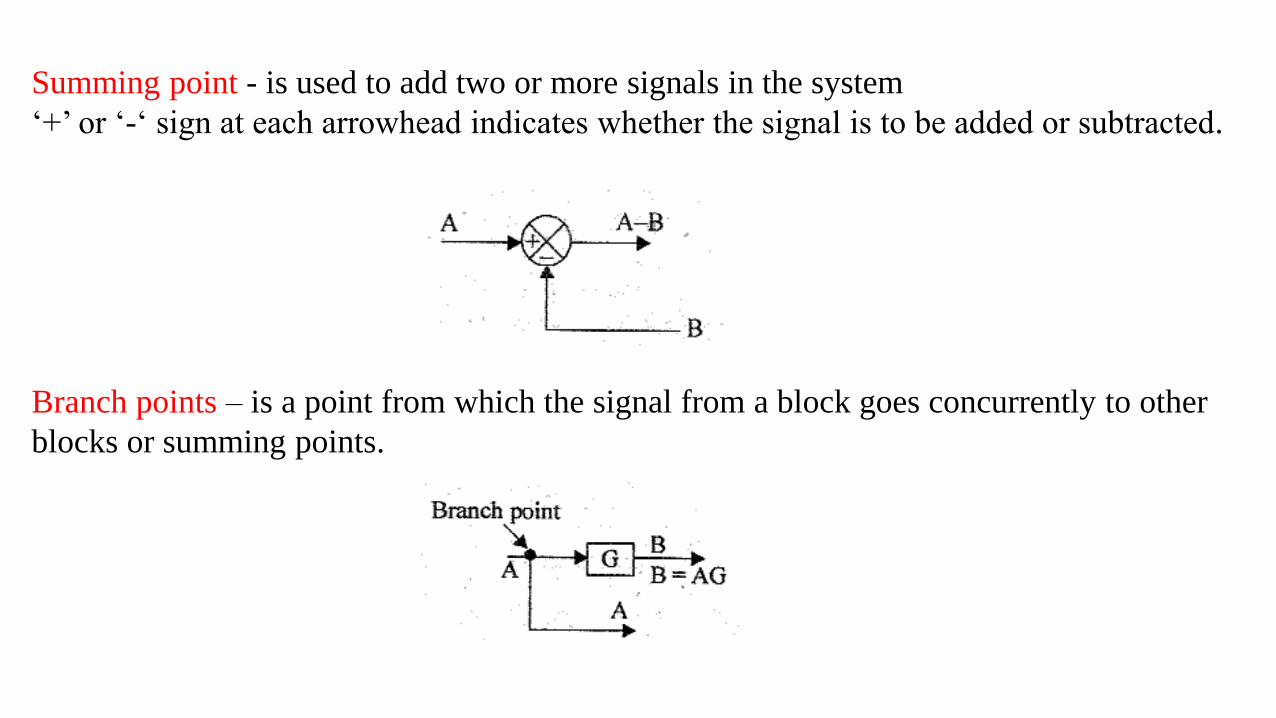
Summing point - is used to add two or more signals in the system

‘+’ or ‘-‘ sign at each arrowhead indicates whether the signal is to be added or subtracted.

Branch points – is a point from which the signal from a block goes concurrently to other

blocks or summing points.

BLOCK DIAGRAM REDUCTION

The block diagram can be reduced to find the overall transfer function of the system.

Rules of block diagram algebra

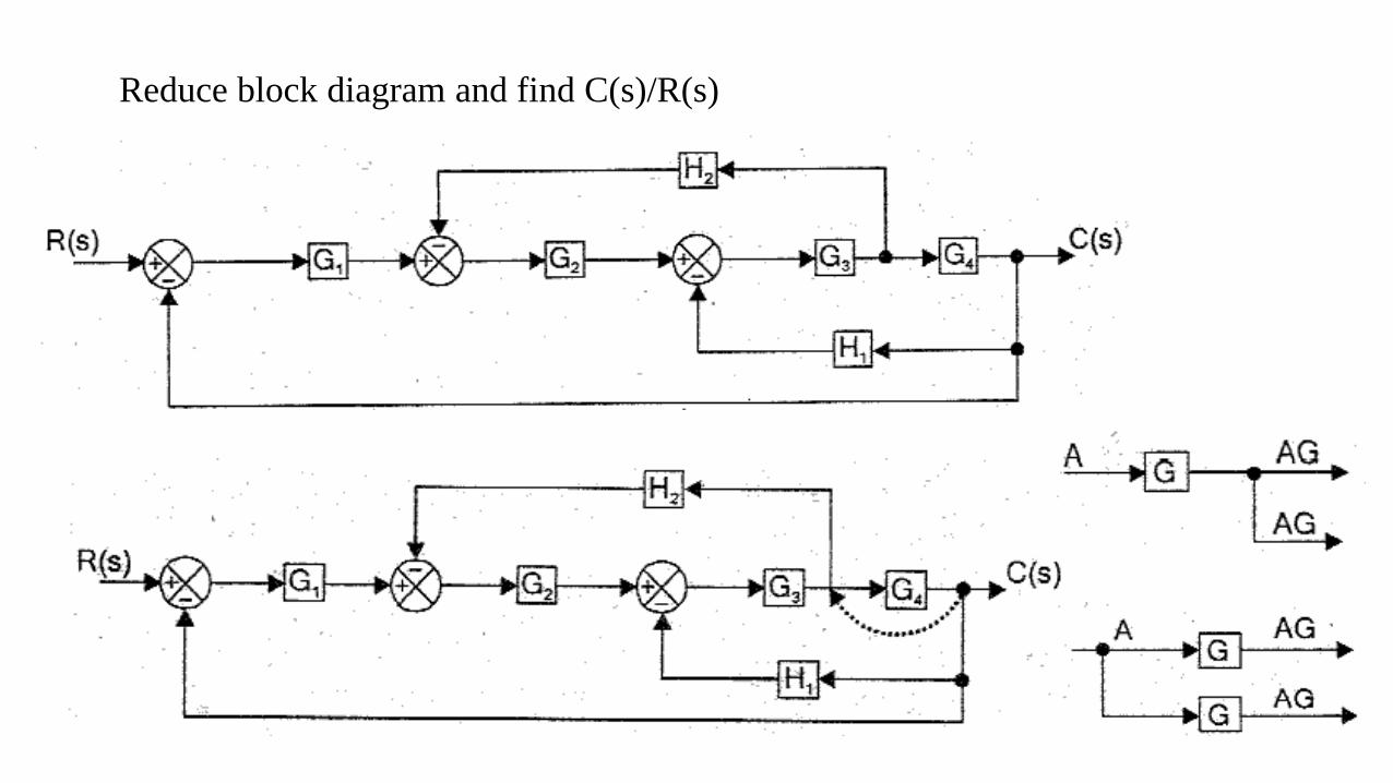
Reduce block diagram and find C(s)/R(s)

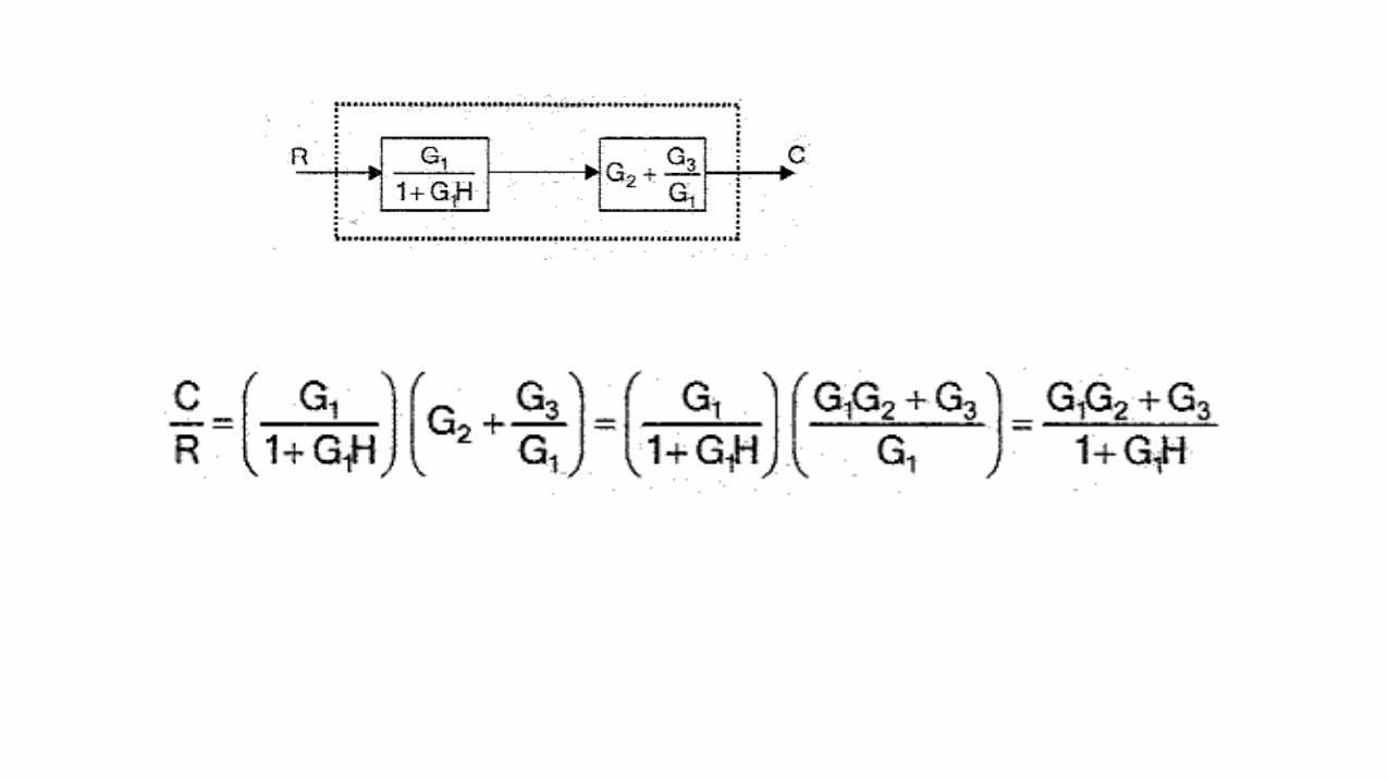
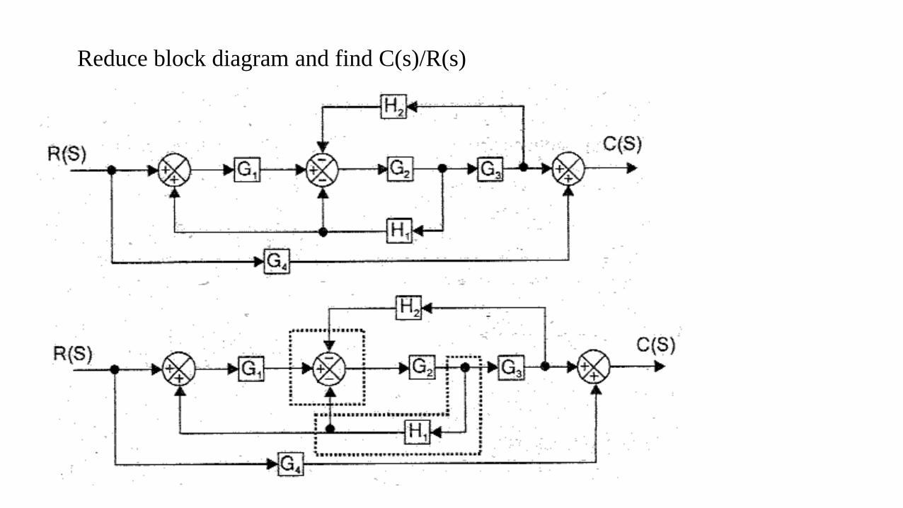
Reduce block diagram and find C(s)/R(s)

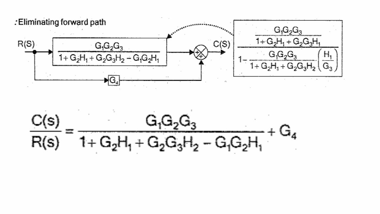
Reduce block diagram and find C(s)/R(s)

TRANSFER FUNCTION OF ARMATURE CONTROLLED DC MOTOR

The speed of DC motor is directly proportional to armature voltage

and inversely proportional to flux in the field winding

In armature controlled DC motor the desired speed is obtained by

varying the armature voltage

This speed control system is an electromechanical control system

The electrical system consists of armature and field circuit but for analysis purpose only

the armature circuit is considered because the field is excited by a constant voltage.

The mechanical system consists of the rotating part of the motor and

load connected to the shaft of the motor

Armature controlled DC motor

Armature equivalent circuit

By Kirchoff’s voltage law

Torque of DC motor is proportional to the product of flux and current

2

1

The mechanical system of the motor

The differential equation governing the mechanical system of motor

The back EMF of DC machine is proportional to speed of shaft

3

4

Take the Laplace Transform of all equation

From equation 6 & 7

7

6

9

8

5

On rearranging Va(S)

Substitute the values of Ia(S) and Eb(S) in equation 10

10

The required function is

TRANSFER FUNCTION OF FIELD CONTROLLED DC MOTOR

The speed of DC motor is directly proportional to armature voltage and inversely

proportional to flux

In field controlled DC motor the armature voltage is kept constant and the speed is

varied by varying the flux of the machine.

Since flux is directly proportional to field current, the flux is varied by varying field

current.

The speed control system is an electromechanical control system

The electrical system consists of armature and field circuit but for analysis purpose only

field circuit is considered because the armature is excited by a constant voltage.

The mechanical system consists of the rotating part of the motor and the load connected

to the shaft of the motor

The torque of DC motor is proportional to product of flux and armature current.

Since armature current is constant in this system, the torque is proportional to flux

alone, but flux is proportional to field current

1

2

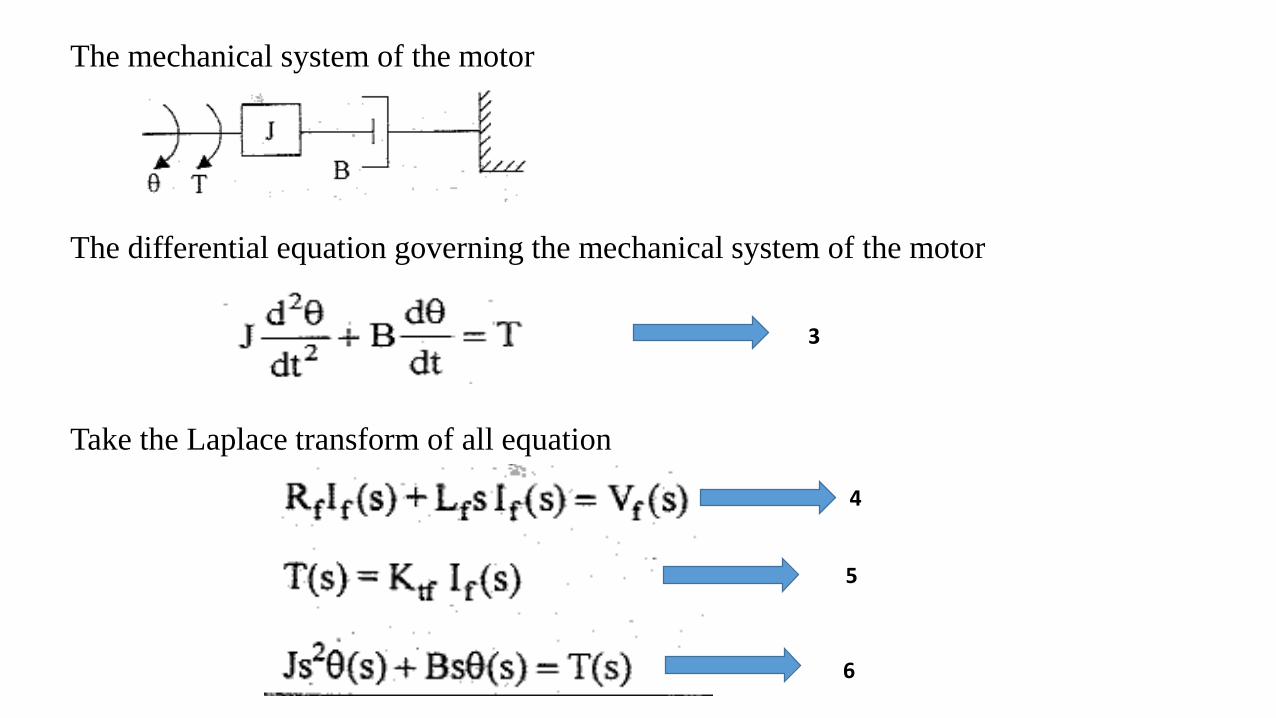
The mechanical system of the motor

The differential equation governing the mechanical system of the motor

Take the Laplace transform of all equation

3

4

5

6

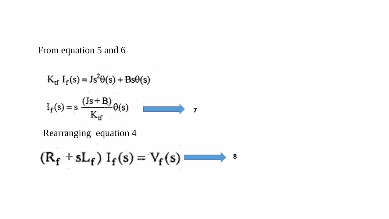
From equation 5 and 6

Rearranging equation 4

7

8

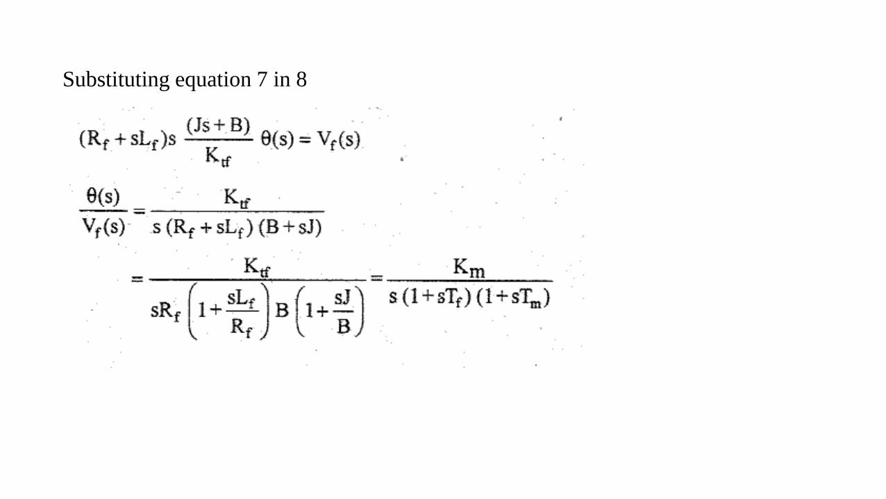
Substituting equation 7 in 8

Where

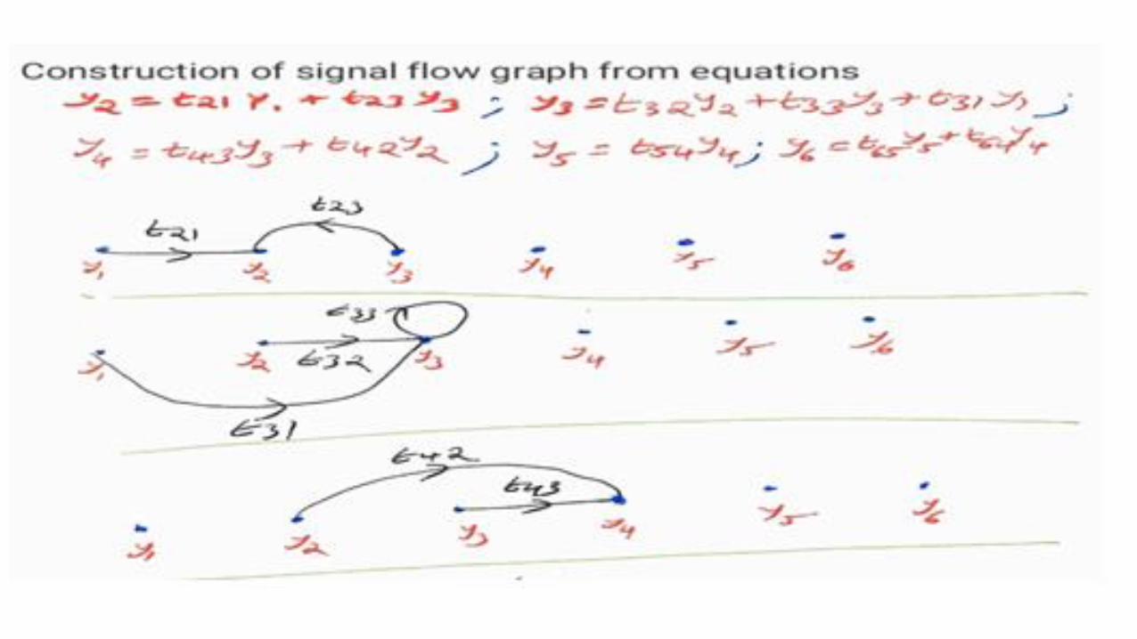
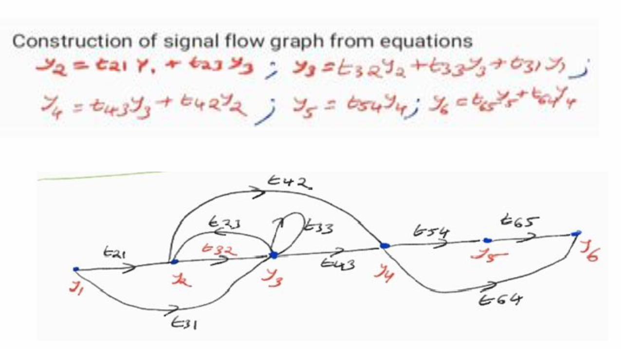
SIGNAL FLOW GRAPH

The signal flow graph is used to represent the control system graphically and it was developed

by S J mason

A signal flow graph is a diagram that represents a set of simultaneous linear algebraic equations

The advantage in signal flow graph method is that, using mason's gain formula the overall gain

of the system can be computed easily.

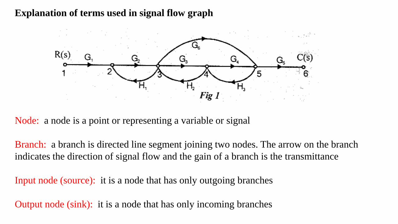
Explanation of terms used in signal flow graph

Node: a node is a point or representing a variable or signal

Branch: a branch is directed line segment joining two nodes. The arrow on the branch

indicates the direction of signal flow and the gain of a branch is the transmittance

Input node (source): it is a node that has only outgoing branches

Output node (sink): it is a node that has only incoming branches

Explanation of terms used in signal flow graph

Mixed node: it is a node that has both incoming and outgoing branches

Path: a path is a traversal of connected branches in the direction of the branch arrows. The

path should not cross a node more than once

Open path: a open path starts at a node and ends at another node

Closed path: closed path starts and ends at same node

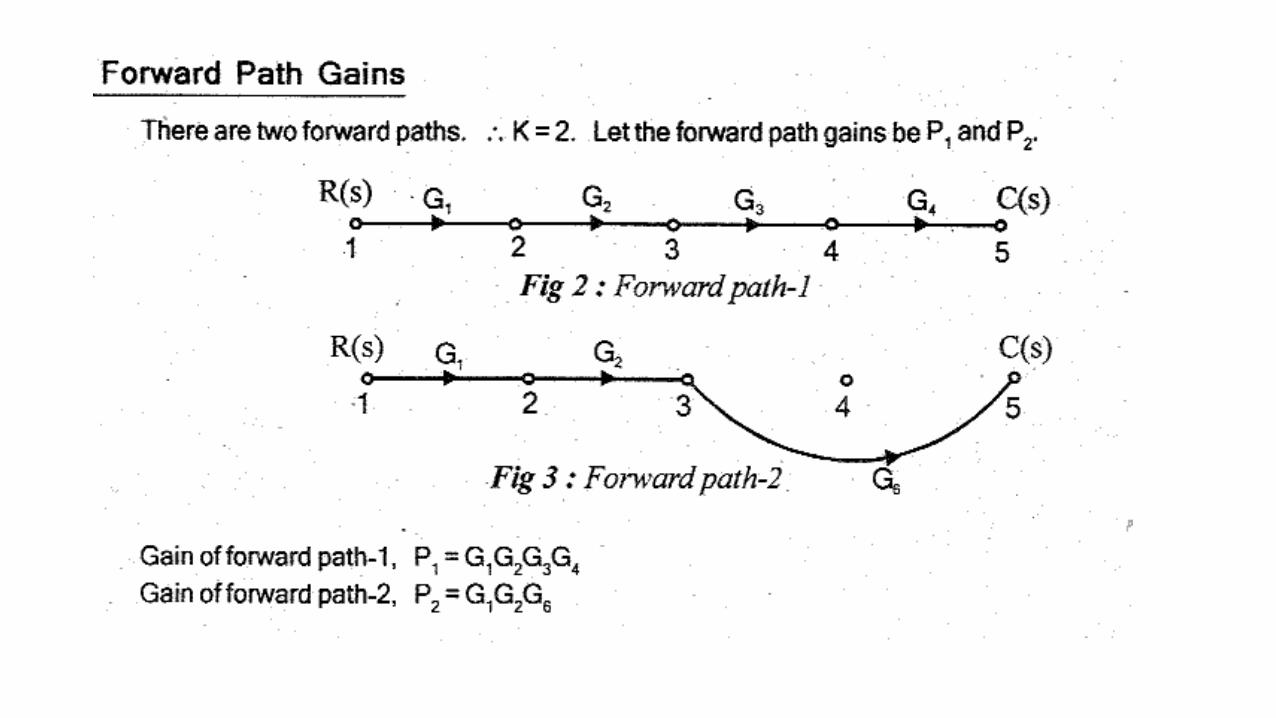
Forward path: it is a path from an input node to an output node that does not cross any node

more than once

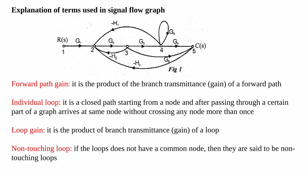
Explanation of terms used in signal flow graph

Forward path gain: it is the product of the branch transmittance (gain) of a forward path

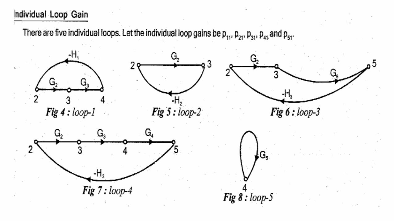
Individual loop: it is a closed path starting from a node and after passing through a certain

part of a graph arrives at same node without crossing any node more than once

Loop gain: it is the product of branch transmittance (gain) of a loop

Non-touching loop: if the loops does not have a common node, then they are said to be non-

touching loops

Properties of signal flow graph

Signal flow graph is applicable to linear time invariant systems

The signal flow is only along the direction of arrows

The value of variable at each node is equal to the algebraic sum of all signals entering at that

node

The gain of signal flow graph is given by Mason's gain formula

The signal gets multiplied by the branch gain when it travels along it

The signal flow graph is not be the unique property of the system

Comparison of block diagram and signal flow graph method

Sl.No Block diagram SFG

1 applicable to Linear time invariant systems applicable to Linear time invariant

systems

2 each element is represented by block each variable is represented by node

3 summing point and take off points are

separate

summing and take off points are

absent

4 self-loop do not exist self-loop can be exist

5 it is time consuming method require less time by using Mason gain

formula

6 block diagram is required at each and every

step

at each step it is not necessary to

draw SFG

7 Only transfer function of the element is shone

inside the corresponding block

transfer function is shown along the

branches connecting the nodes

8 feedback path is present feedback loops are used

Module II

1. Control system components: DC and AC servo motors – synchro - gyroscope - stepper

motor - Tacho generator.

2. Time domain analysis of control systems:

a. Transient and steady state responses

b. Test signals

c. Order and type of systems

d. Step responses of first and second order systems.

e. Time domain specifications

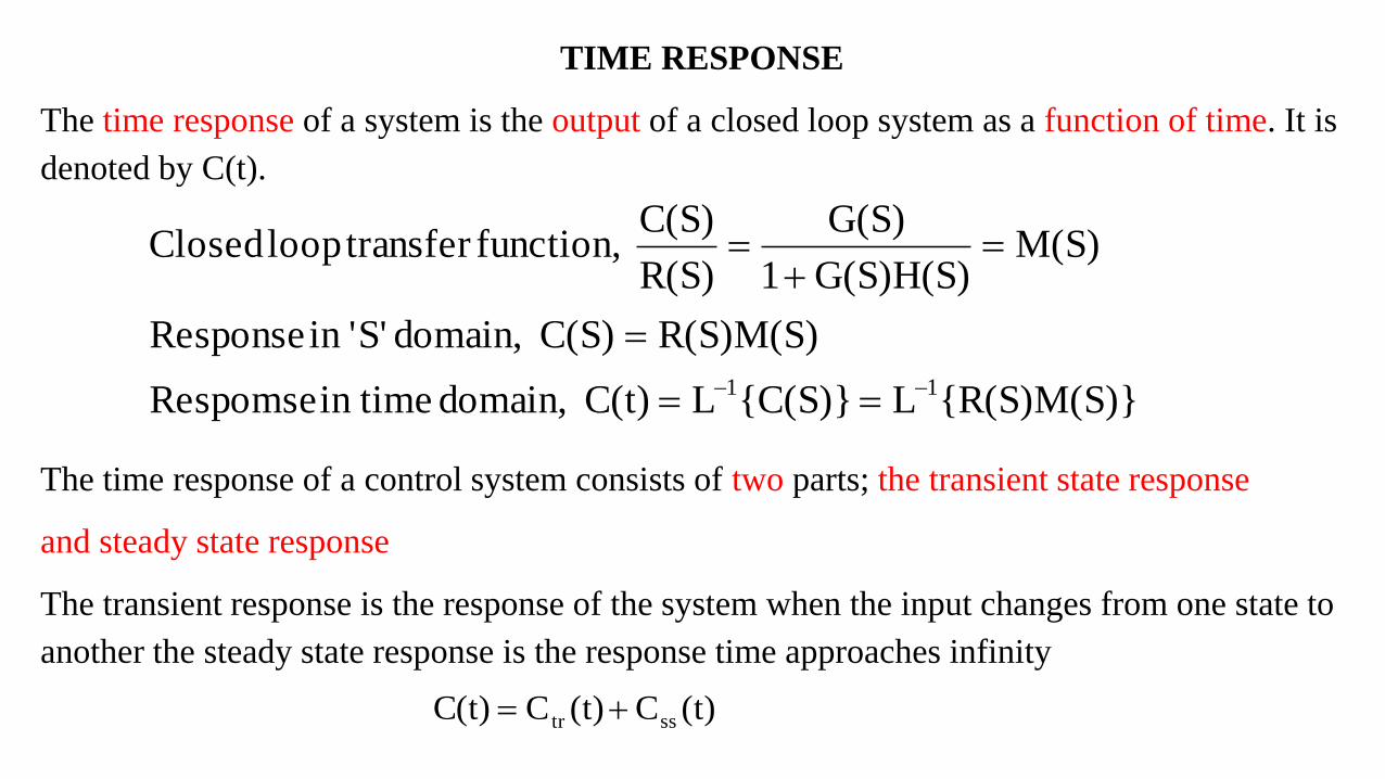
TIME RESPONSE

The time response of a system is the output of a closed loop system as a function of time. It is

denoted by C(t).

The time response of a control system consists of two parts; the transient state response

and steady state response

The transient response is the response of the system when the input changes from one state to

another the steady state response is the response time approaches infinity

{R(S)M(S)}L{C(S)}LC(t) domain, in time Respomse

R(S)M(S)C(S) domain, S''in Response

M(S)G(S)H(S)1

G(S)

R(S)

C(S) function, transfer loop Closed

11

(t)C(t)CC(t) sstr

(t)C(t)CC(t) sstr

TEST SIGNALS

The characteristics of actual input signals are a sudden shock, a sudden change, a constant

velocity and a constant acceleration.

Test signals which resembles these characteristics are used as input signal to predict the

performance of the system.

The standard test signals are step signal, unit step signal, unit ramp signal, ramp signal, unit

impulse signal and sinusoidal signal

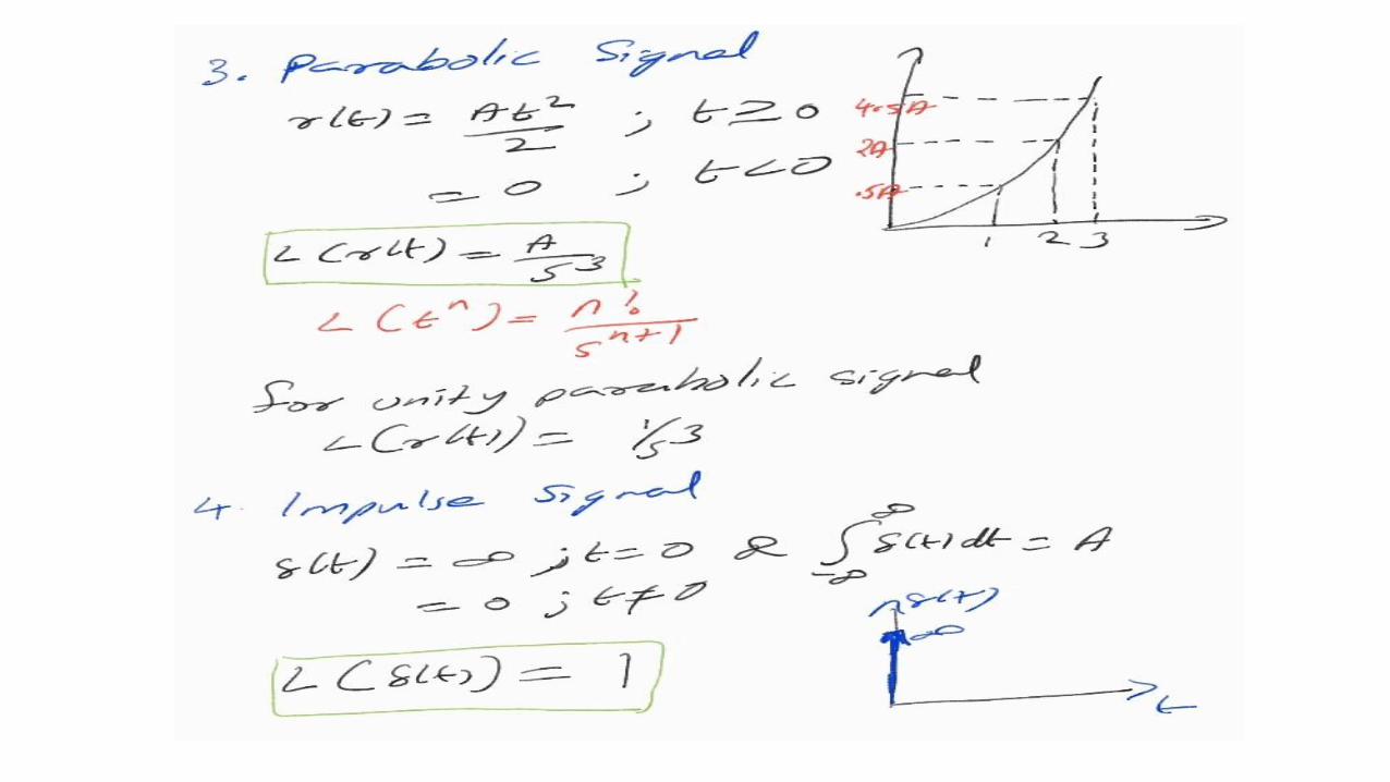
IMPULSE SIGNAL

A signal of very large magnitude which is available for very short duration is called Impulse

signal

Ideal impulse signal is a signal with infinite magnitude and zero duration but with an area of

A.

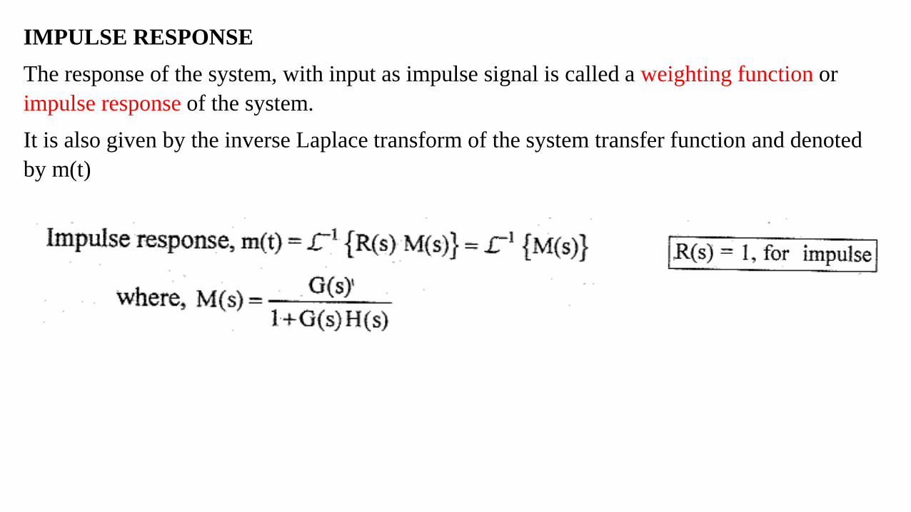
IMPULSE RESPONSE

The response of the system, with input as impulse signal is called a weighting function or

impulse response of the system.

It is also given by the inverse Laplace transform of the system transfer function and denoted

by m(t)

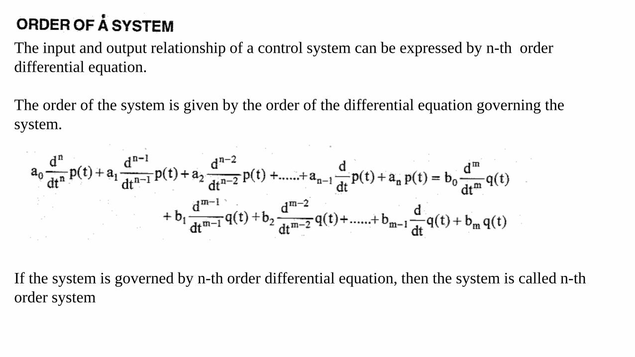
The input and output relationship of a control system can be expressed by n-th order

differential equation.

The order of the system is given by the order of the differential equation governing the

system.

If the system is governed by n-th order differential equation, then the system is called n-th

order system

The order can also be determined from the transfer function of the system.

The order of the system is given by the maximum power of ‘S’ in the denominator

polynomial

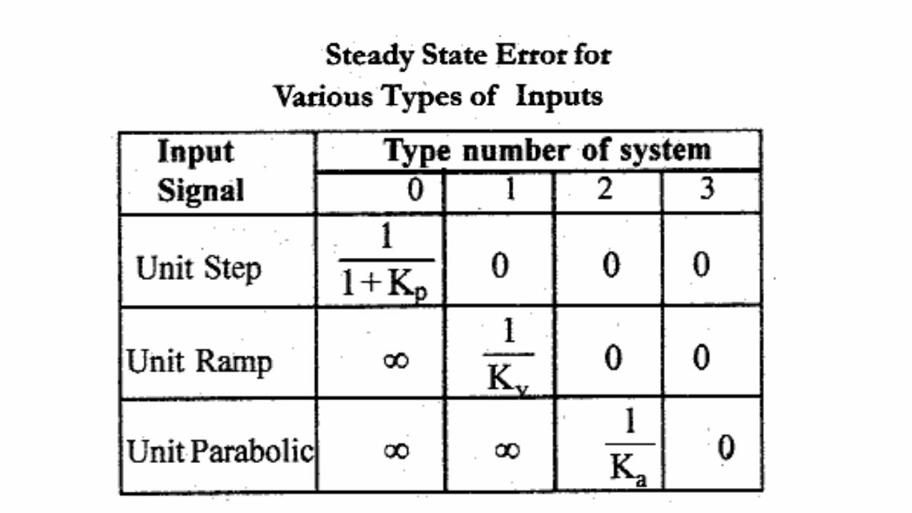
TYPE NUMBER OF CONTROL SYSTEMS

The type number is specified for loop transfer function G(S)H(S).

The number of poles of the loop transfer function lying at the origin decides the type number of

the system

In general if ‘N’ is the number of poles at the origin then the type number is ‘N’

TYPE NUMBER OF CONTROL SYSTEMS

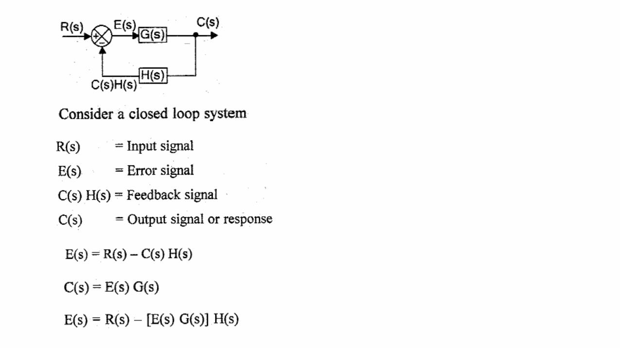
Response of first order system for unit step input

The closed loop first order system with unity feedback is

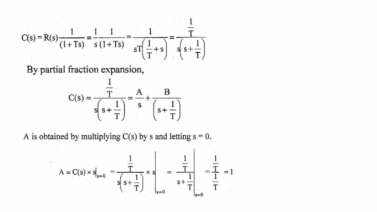
When

The damping ratio is defined as the ratio of the actual damping to the critical damping.

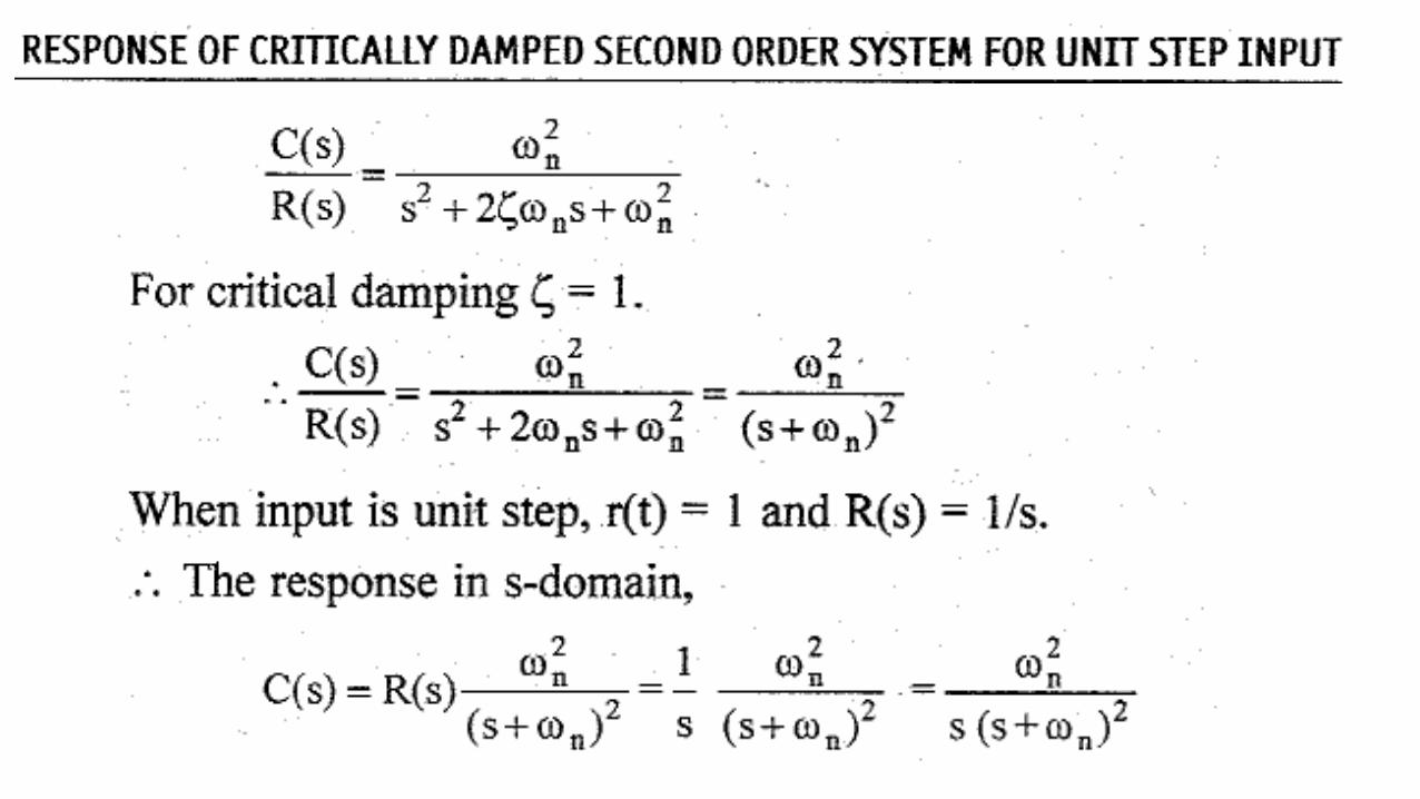
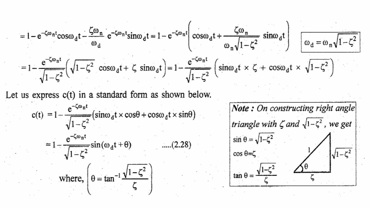
The response C(t) of second order system depends on the value of damping ratio.

Depending on the value of damping ratio, the system can be classified into four.

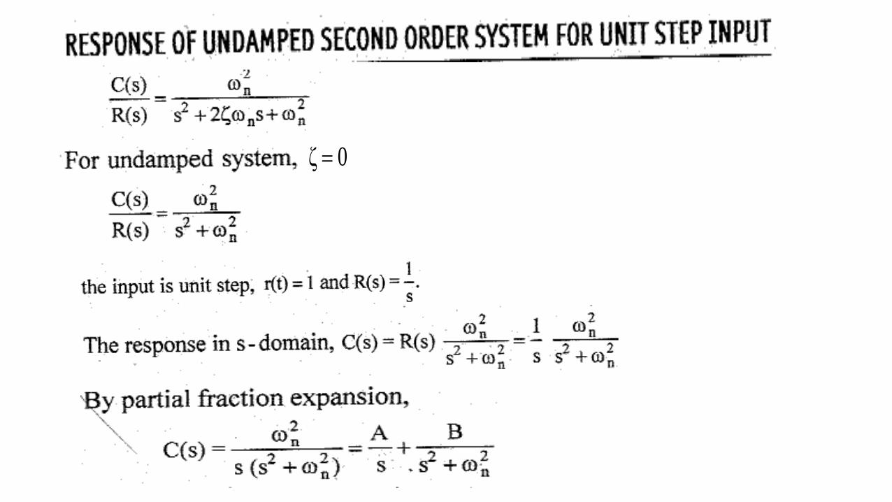
0ζ

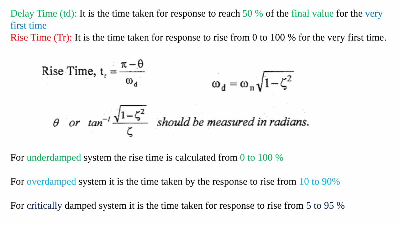
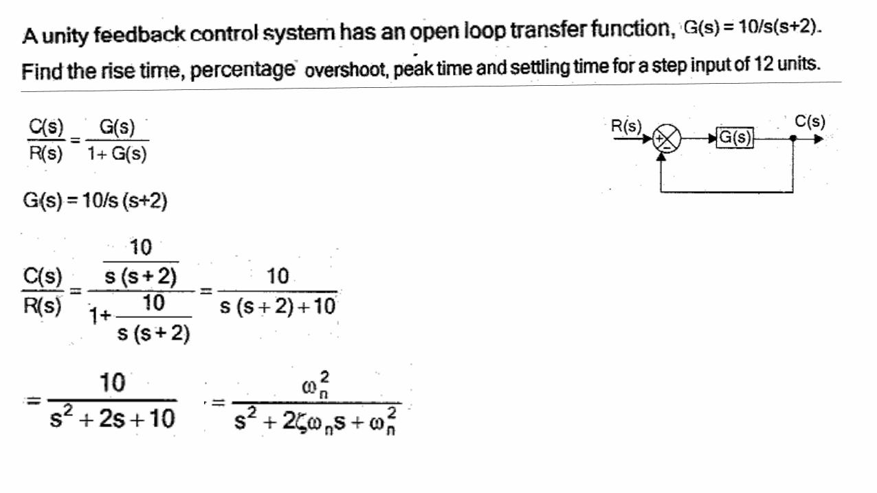
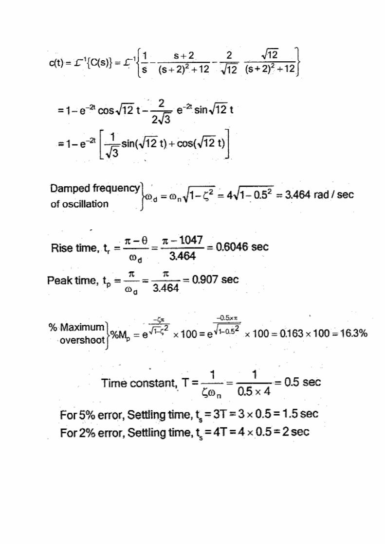
Delay Time (td): It is the time taken for response to reach 50 % of the final value for the very

first time

Rise Time (Tr): It is the time taken for response to rise from 0 to 100 % for the very first time.

For underdamped system the rise time is calculated from 0 to 100 %

For overdamped system it is the time taken by the response to rise from 10 to 90%

For critically damped system it is the time taken for response to rise from 5 to 95 %

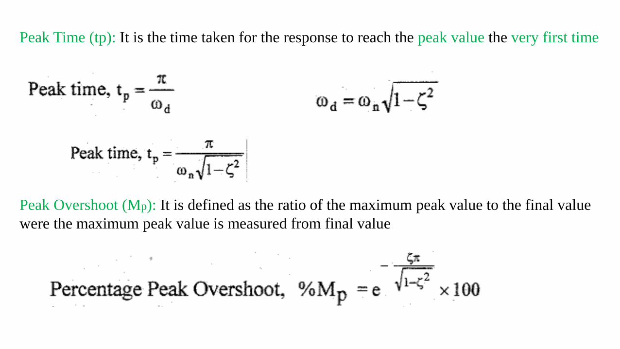
Peak Time (tp): It is the time taken for the response to reach the peak value the very first time

Peak Overshoot (Mp): It is defined as the ratio of the maximum peak value to the final value

were the maximum peak value is measured from final value

Settling Time (ts): It is defined as the time taken by the response to reach and stay within a

specified error.

It is usually expressed as percentage of final value.

The usual tolerable error is 2% or 5% of the final value.

error) T.ln(%- ζω

error) ln(%-)(t timeSettling

n

s

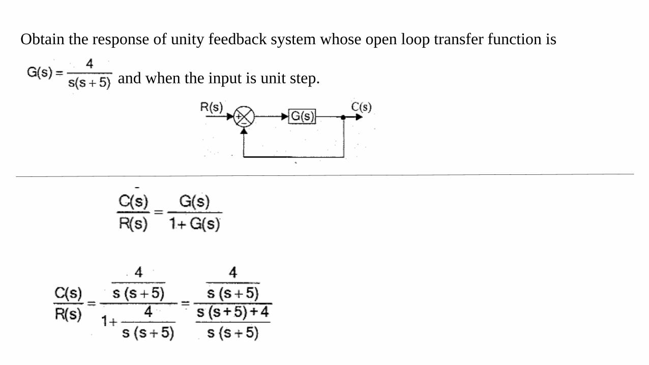
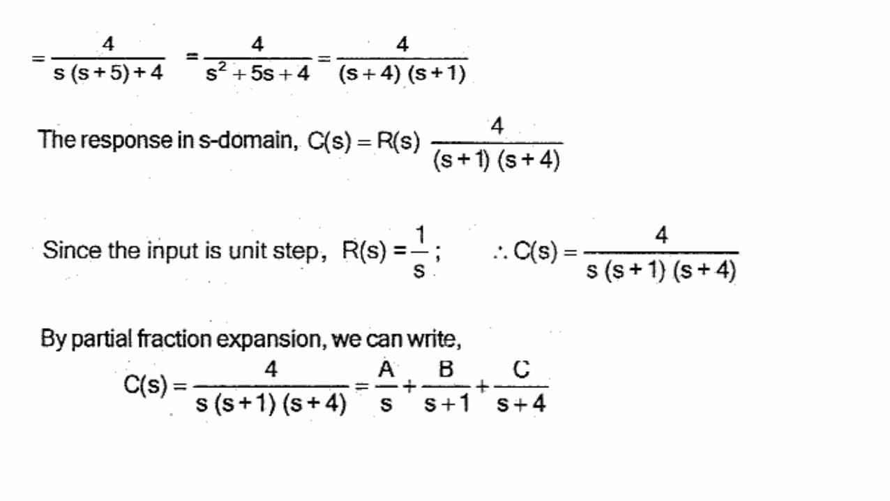
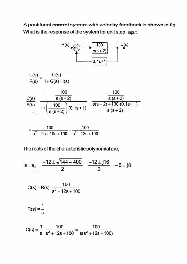
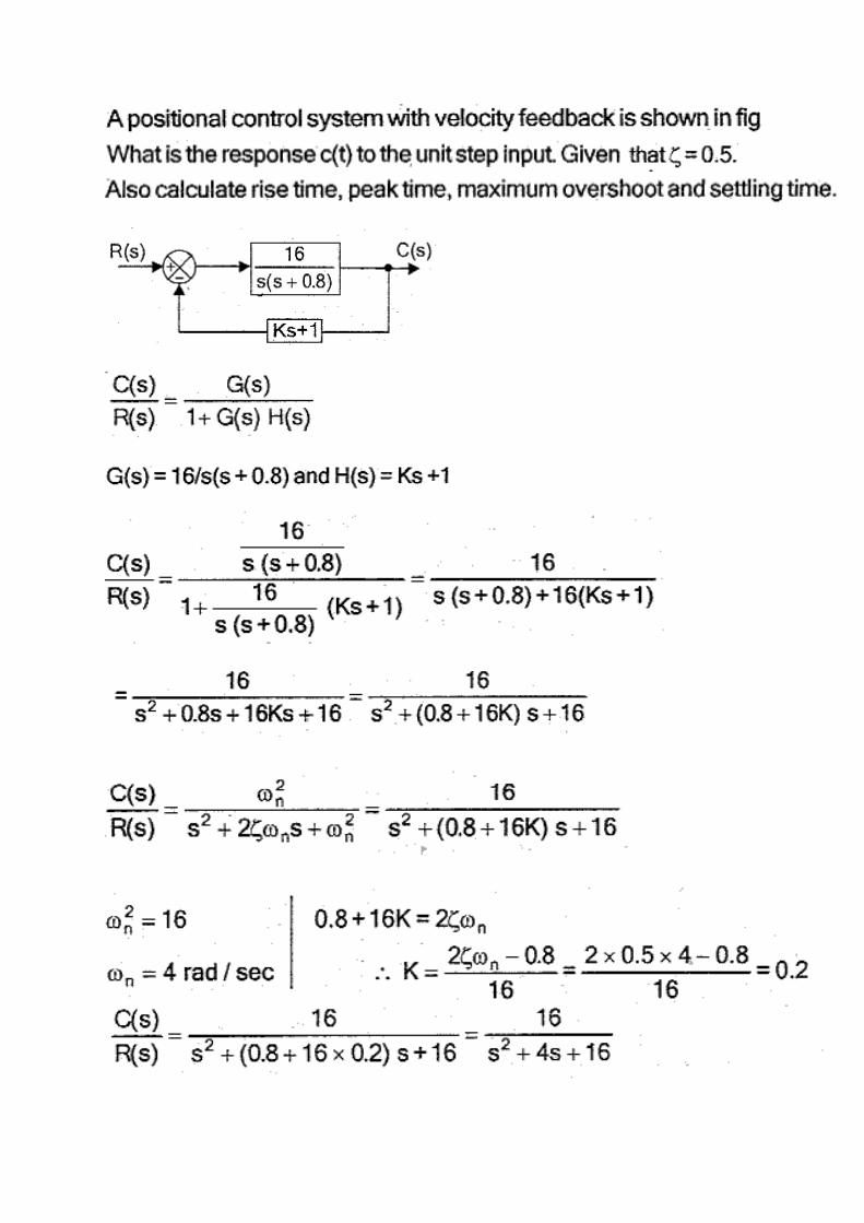
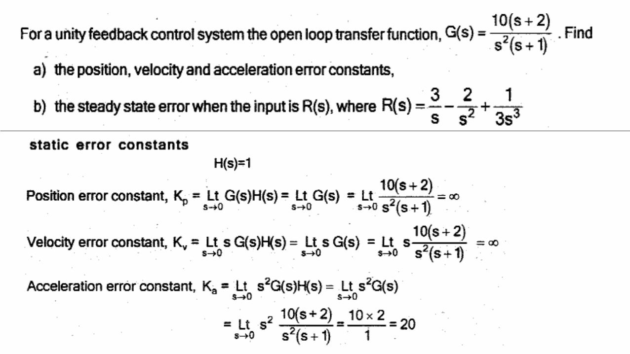
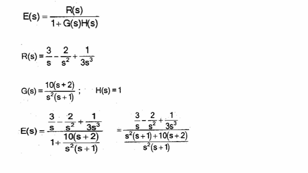
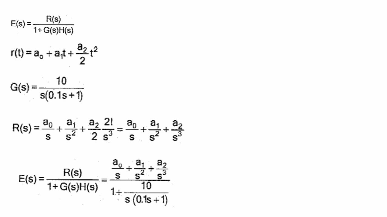
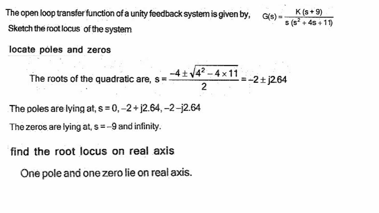
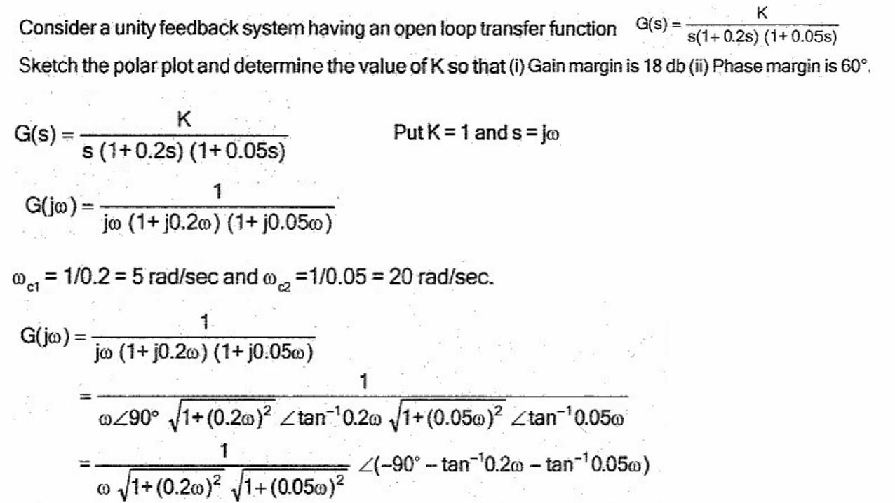
Obtain the response of unity feedback system whose open loop transfer function is

and when the input is unit step.

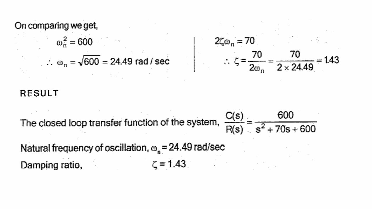
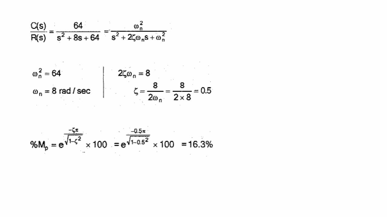
The response of a servomechanism is when subject to a unit

step input. Obtain an expression for closed loop transfer function. Determine the undamped

natural frequency and damping ratio.

Take the Laplace transform

10t60t 1.2e0.2e1c(t)

10t60t 1.2e0.2e1c(t)

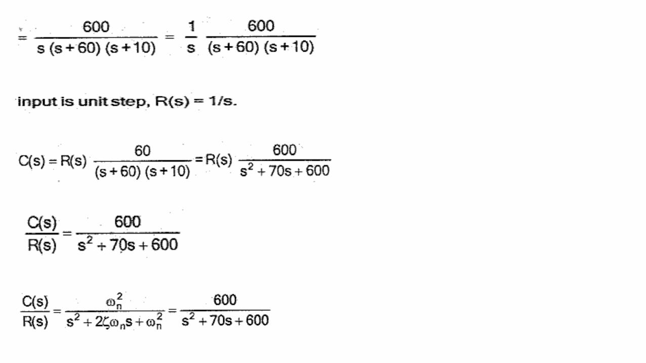
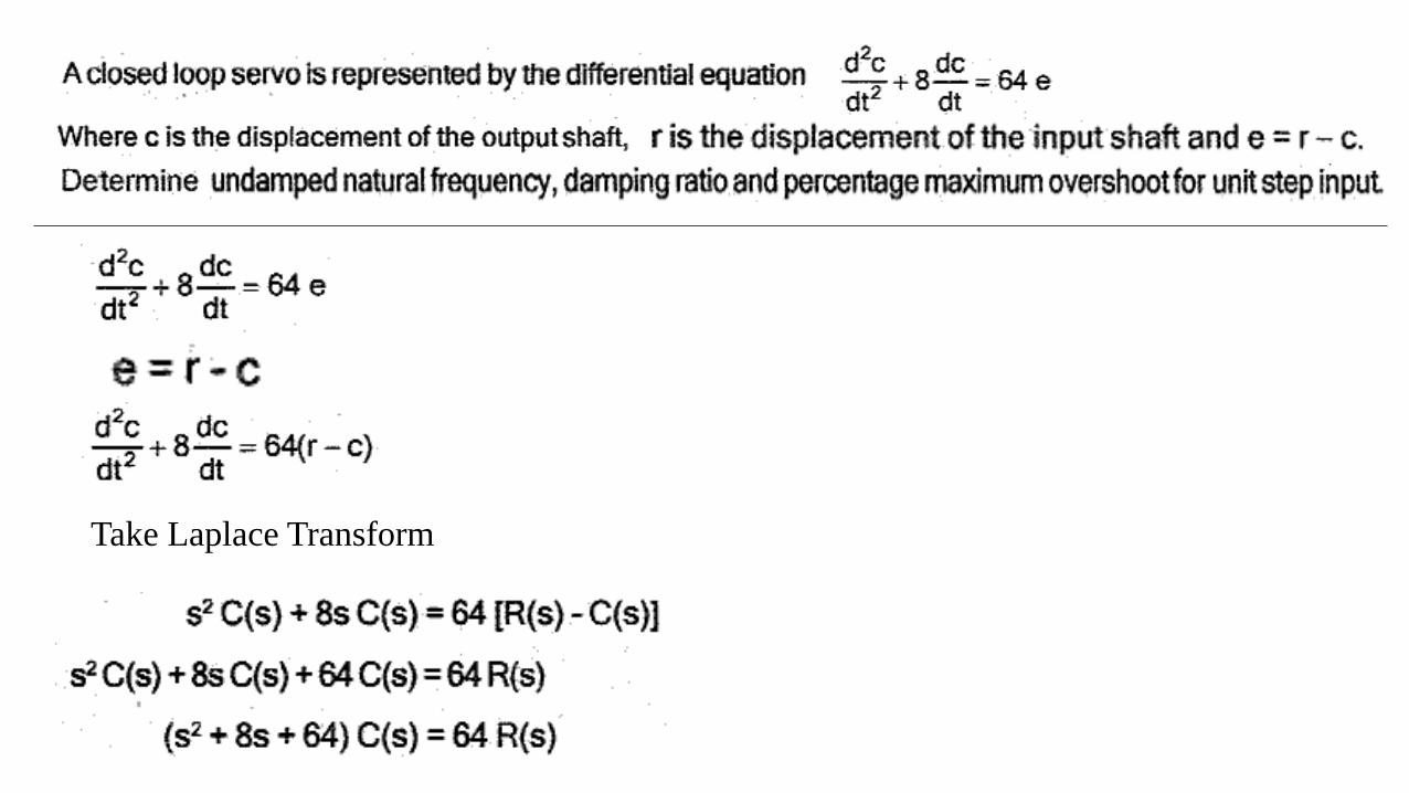
Take Laplace Transform

Module III

Error analysis:

steady state error analysis

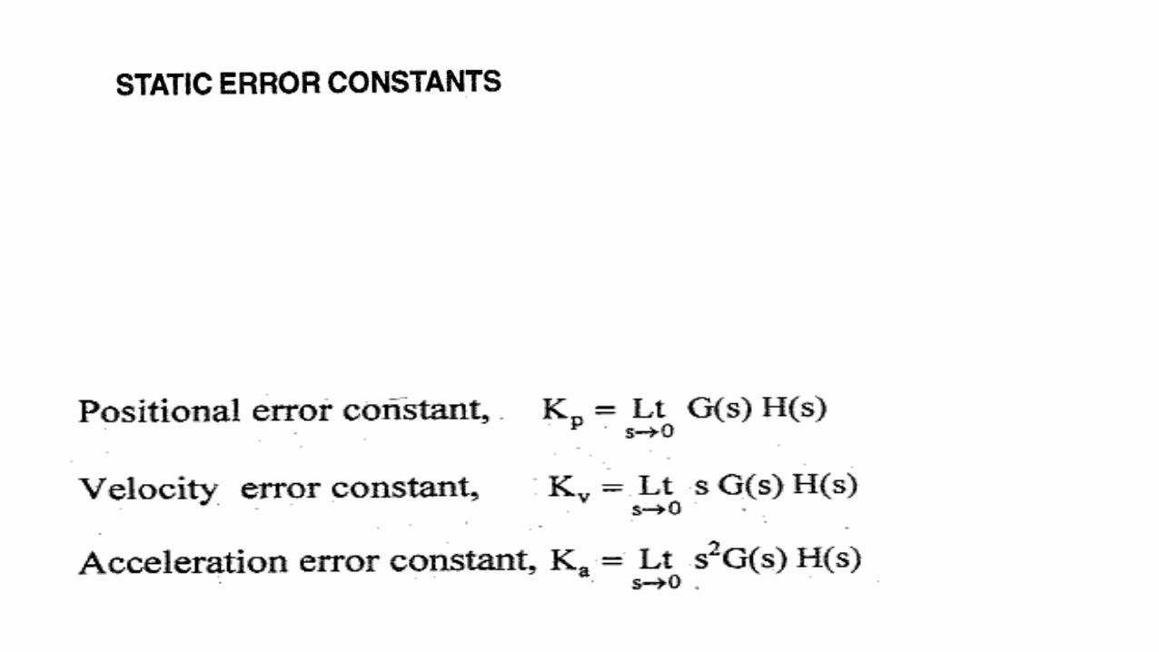
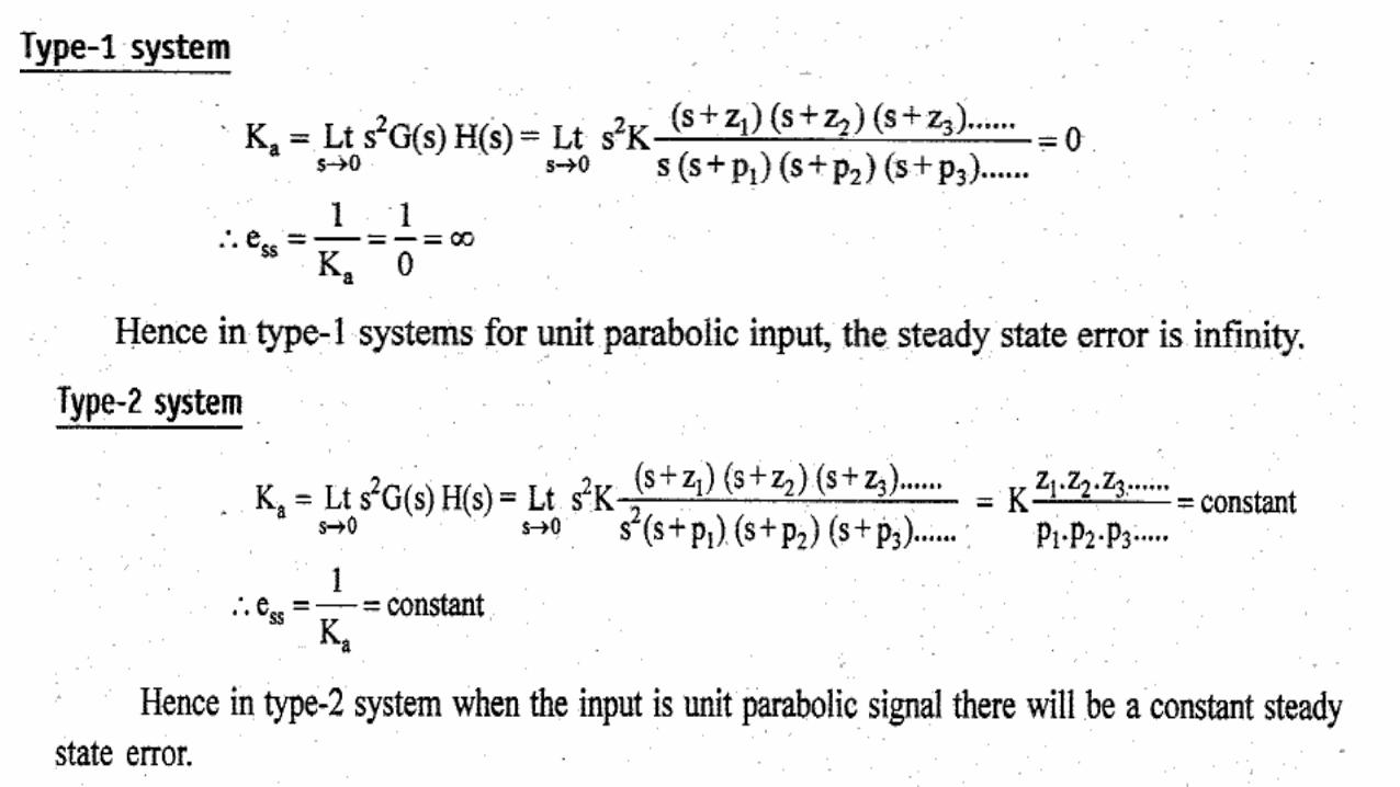
static error coefficient of type 0,1, 2 systems

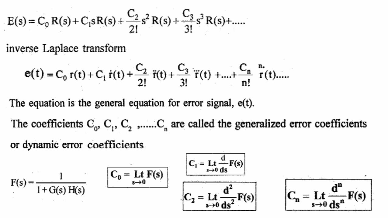
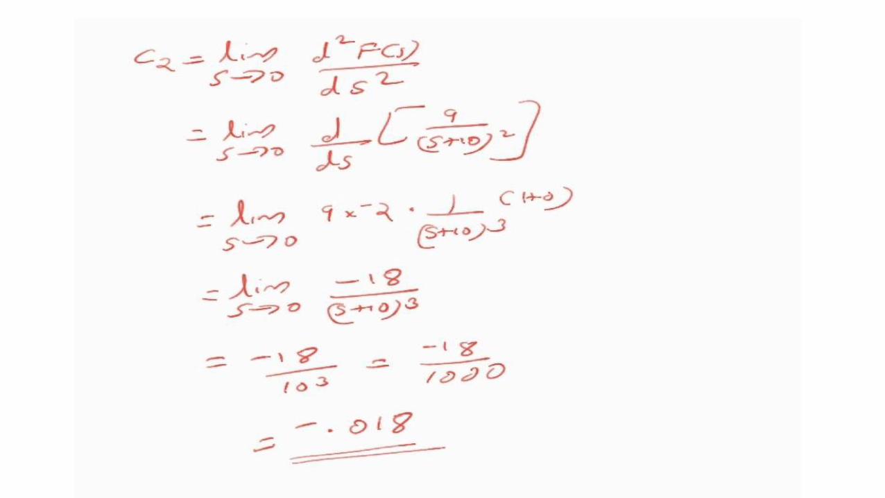
Dynamic error coefficients

Concept of stability:

Time response for various pole locations

stability of feedback system

Routh's stability criterion

The input and output relationship of a control system can be expressed by n-th order

differential equation.

The order of the system is given by the order of the differential equation governing the

system.

If the system is governed by n-th order differential equation, then the system is called n-th

order system

The order can also be determined from the transfer function of the system.

The order of the system is given by the maximum power of ‘S’ in the denominator

polynomial

TYPE NUMBER OF CONTROL SYSTEMS

The type number is specified for loop transfer function G(S)H(S).

The number of poles of the loop transfer function lying at the origin decides the type number of

the system

In general if ‘N’ is the number of poles at the origin then the type number is ‘N’

TYPE NUMBER OF CONTROL SYSTEMS

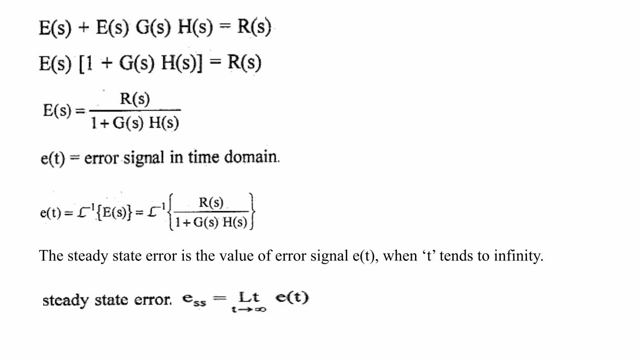
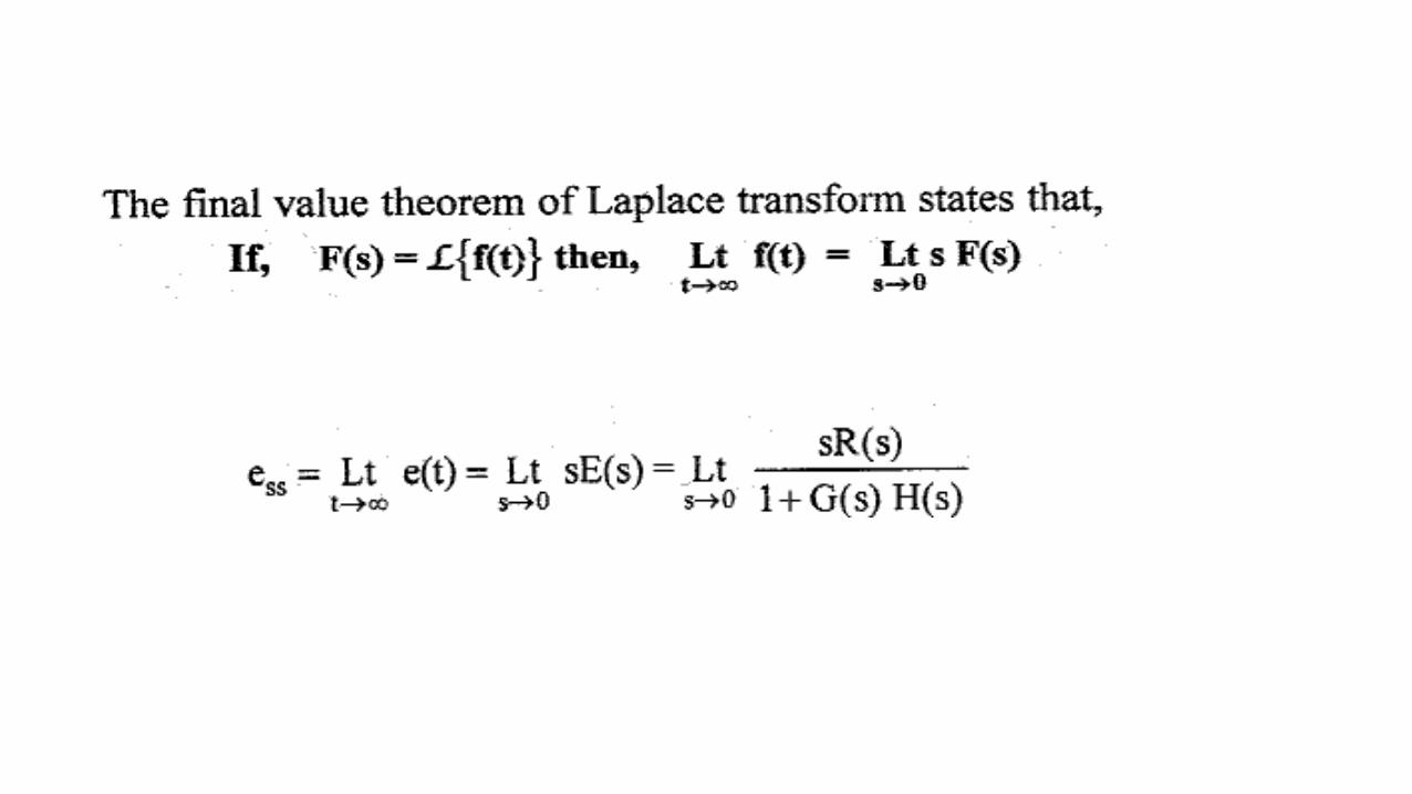
STEADY STATE ERROR

The steady state error is the value of error signal e(t), when ‘t’ tends to infinity.

Steady state error is a measure of system accuracy.

These errors arise from the nature of in inputs, type of system and from non linearity of system

components.

The steady-state performance of a stable control system is generally judged by its steady state

error to step, ramp and parabolic inputs

The steady state error is the value of error signal e(t), when ‘t’ tends to infinity.

STABILITY

The term stability refers to the stable working condition of a control system. Every working

system is designed to be stable. In a stable system the response or output is predictable, finite

and stable for a given input.

The different definition of the stability are the following

1. A system is stable, if its output is bounded (finite) for any bounded (finite) input.

2. A system is asymptotically stable, if in the absence of the input, the output tends towards

zero irrespective of initial conditions.

3. A system is stable if for a bounded disturbing input signal the output vanishes ultimately

as‘t’ approaches infinity.

4. A system is unstable if for a bounded disturbing input signal the output is of finite amplitude

or oscillatory.

5. For a bounded input signal, if the output has constant amplitude of oscillation then the

system may be stable or unstable under some limited constraints. Such a system is called

limitedly stable.

6. If a system output is stable for all variations of its parameters, then the system is called

absolutely stable system.

7. If a system output is stable for a limited range of variations of its parameters, then the

system is called conditionally stable system

SJω

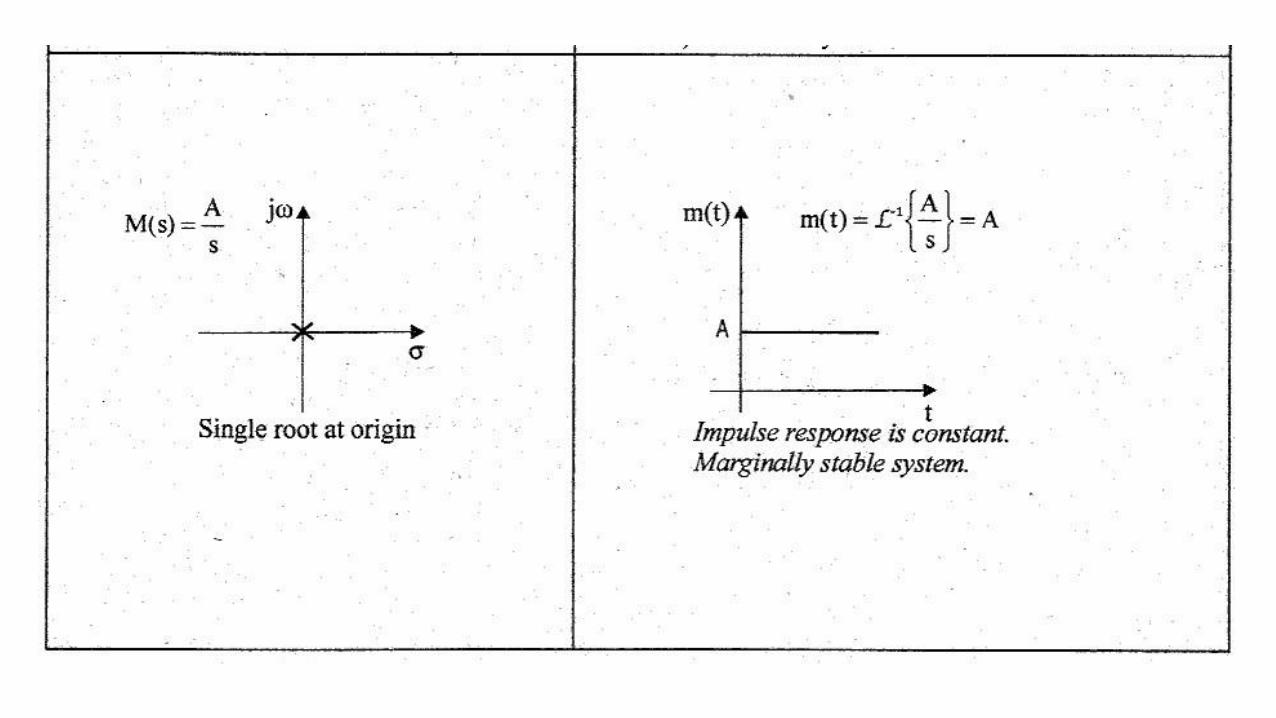
The stability of the system depending on the location of roots of characteristic equation

1. If all the roots of characteristic equation has negative real parts, then the system is stable.

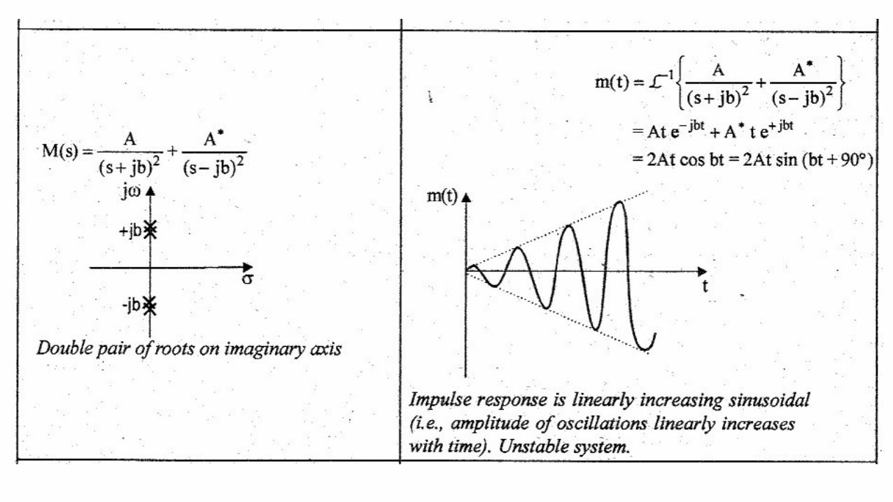
2. If any root of the characteristic equation has a positive real part or if there is a repeated

root on the imaginary axis then the system is unstable.

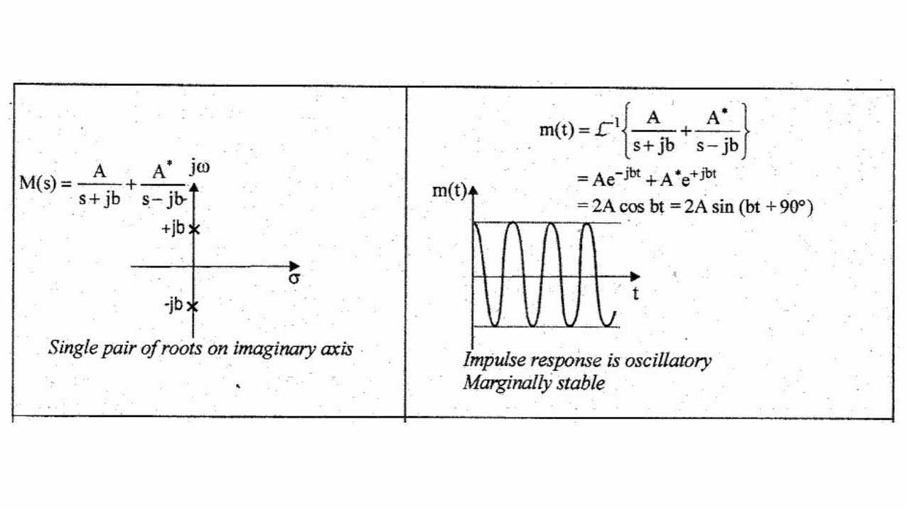
3. If the condition (1) is satisfied except for the presence of one or more non repeated roots

on imaginary axis, then the system is limitedly or marginally stable.

Methods of determining stability

1. Routh-Hurwitz criterion (RH criterion)

2. Bode plot

3. Nyquist criterion

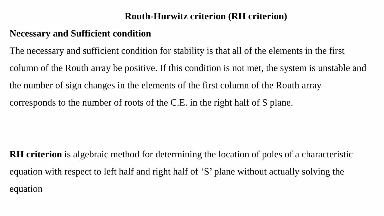
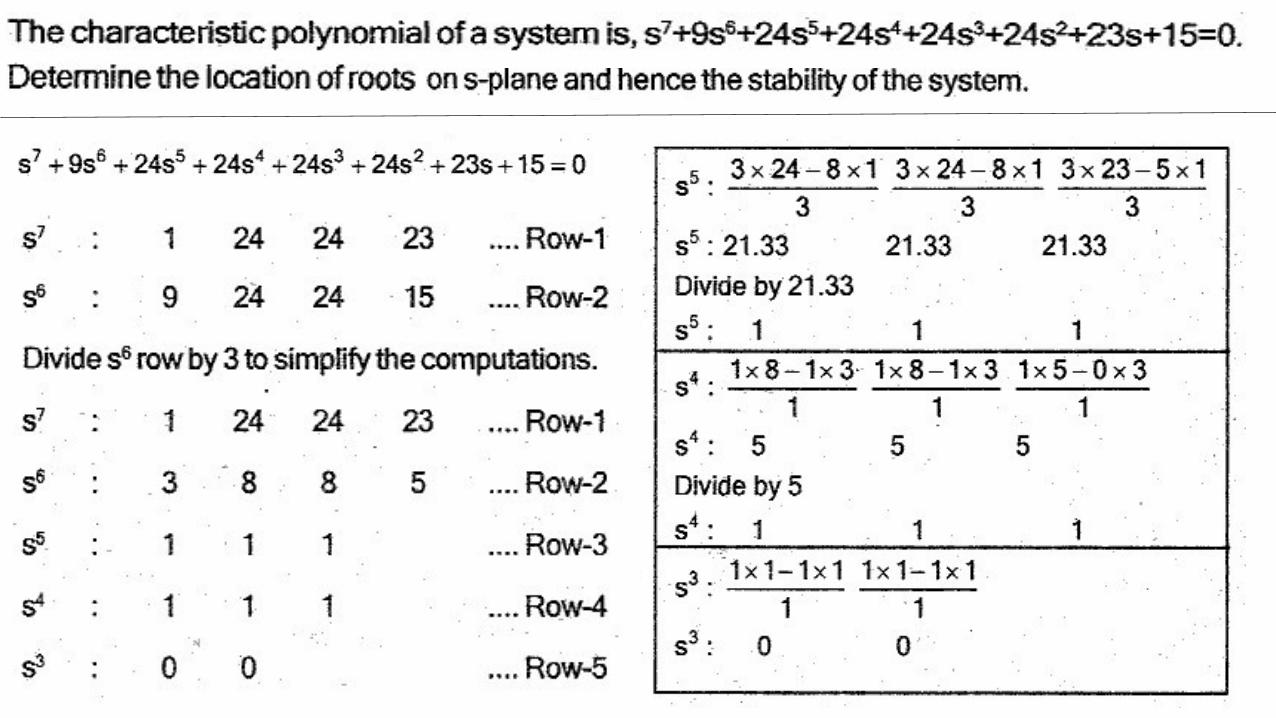
Routh-Hurwitz criterion (RH criterion)

Necessary and Sufficient condition

The necessary and sufficient condition for stability is that all of the elements in the first

column of the Routh array be positive. If this condition is not met, the system is unstable and

the number of sign changes in the elements of the first column of the Routh array

corresponds to the number of roots of the C.E. in the right half of S plane.

RH criterion is algebraic method for determining the location of poles of a characteristic

equation with respect to left half and right half of ‘S’ plane without actually solving the

equation

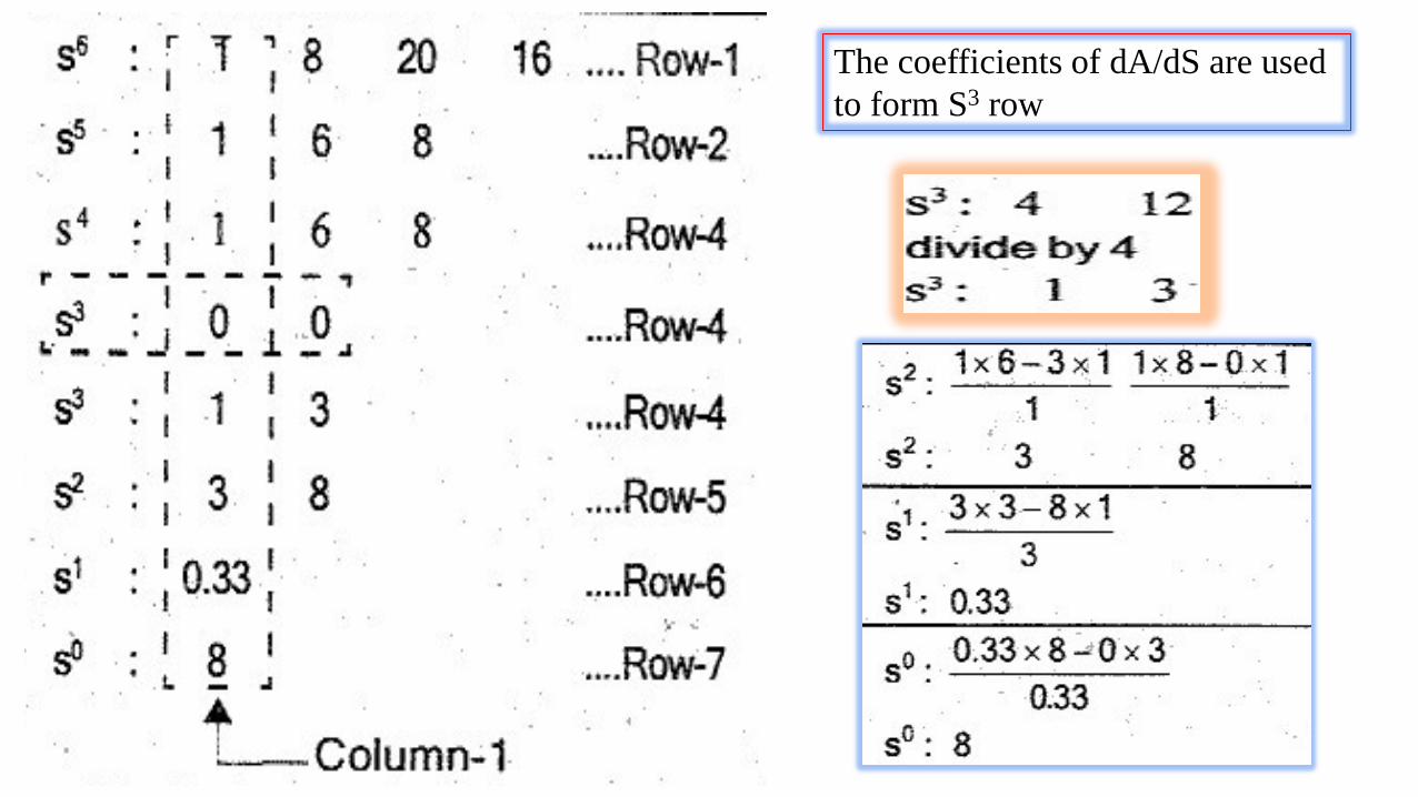
The coefficients of dA/dS are used

to form S3 row

There is no sign change in the first column. The row with all zeros indicate the possibility of

roots on imaginary axis. Hence the system is limitedly or marginally stable.

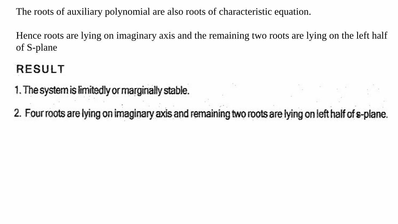
The roots of auxiliary polynomial are also roots of characteristic equation.

Hence roots are lying on imaginary axis and the remaining two roots are lying on the left half

of S-plane

RESULT

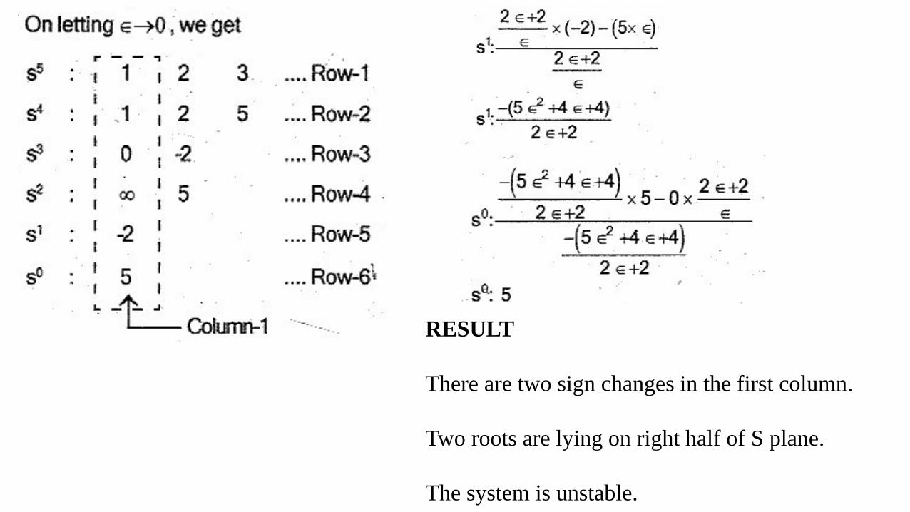
There are two sign changes in the first column.

Two roots are lying on right half of S plane.

The system is unstable.

RESULT

There are three sign changes

Three roots are lying on right half of S plane and Two roots are lying on

left half of S plane

The system is unstable.

The elements of column-1 of quotient polynomial are all positive.

There is no sign change

All the roots of quotient polynomial are lying on the left half of S-plane.

To determine the stability, the roots of auxiliary polynomial should be evaluated

The roots of auxiliary equation are complex.

Two roots of auxiliary equation are lying on the right half of S plane and the other two on the

left half of S plane

RESULT

The roots of auxiliary polynomial is also the roots of C.E.

Hence two roots of C.E are lying on the right half of S plane and remaining five roots are

lying on left half of S plane.

The system is unstable.

MODULE IV

Root locus

General rules for constructing Root loci

Stability from root loci

Effect of addition of poles and zeros.

ROOT LOCUS

Graphical approach

Powerful tool for adjusting the location of closed loop poles to achieve the desired system

performance by varying one or more system parameters.

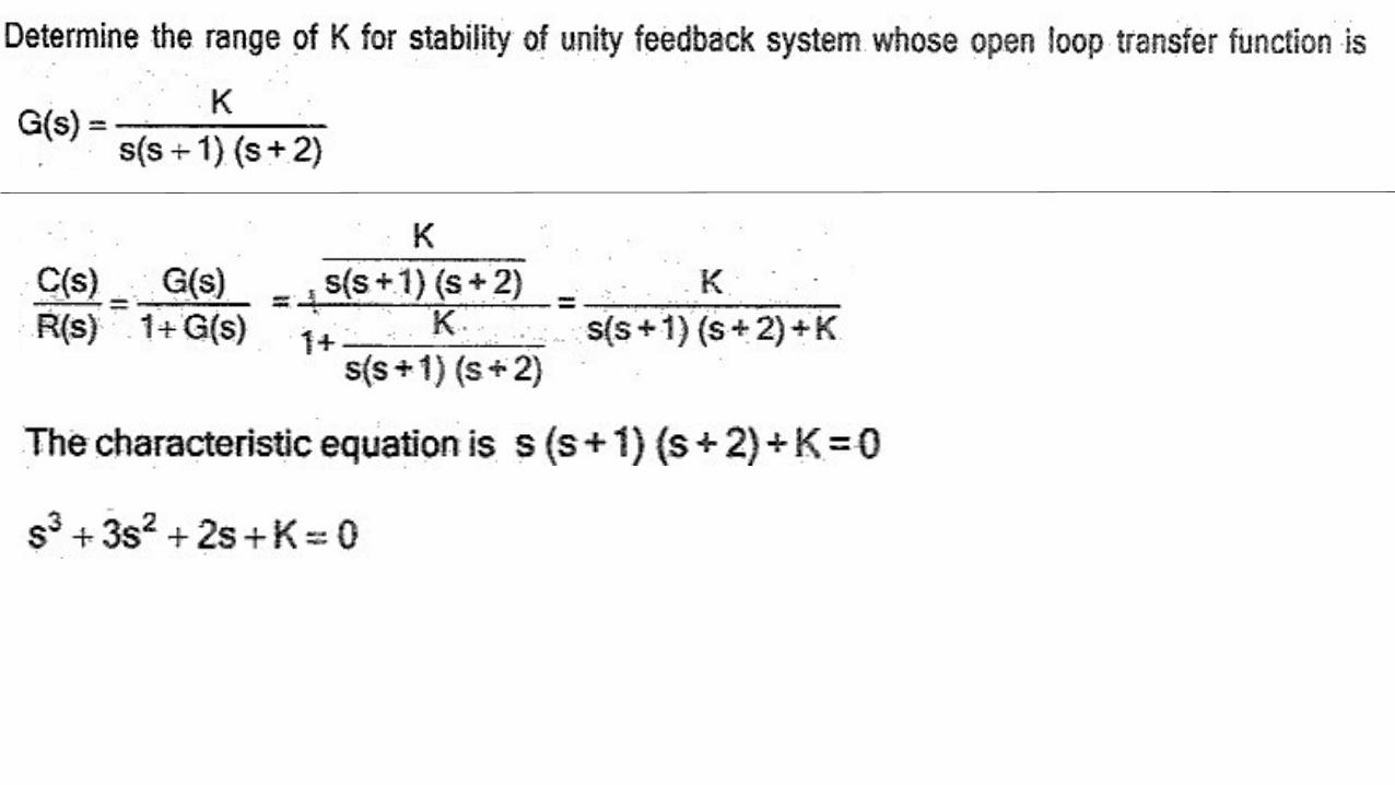
Consider open loop transfer function of the system

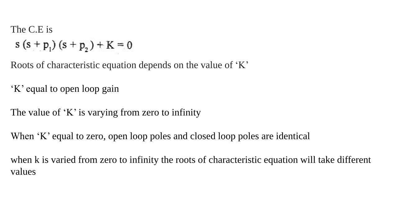
The C.E is

Roots of characteristic equation depends on the value of ‘K’

‘K’ equal to open loop gain

The value of ‘K’ is varying from zero to infinity

When ‘K’ equal to zero, open loop poles and closed loop poles are identical

when k is varied from zero to infinity the roots of characteristic equation will take different

values

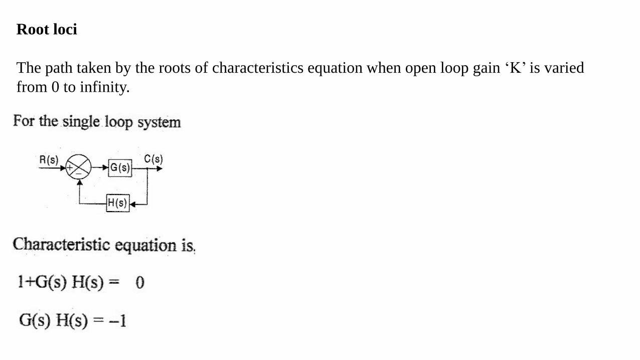
Root loci

The path taken by the roots of characteristics equation when open loop gain ‘K’ is varied

from 0 to infinity.

21212211

21

2

1

22

11

θθθrθr

θθr

r

θr

θr

rr

The open loop gain ‘K’ corresponding to a point S=Sa on root locus can be calculated using

above equation.

is equal to the length of vector drawn from S=Pi to S=Sa

is equal to the length of vector drawn from S=Zi to S=Sa

Hence

Sa=Spoint the tozeros loopopen from vector oflength ofProduct

Sa=Spoint the topoles loop-open from vector oflength ofProduct K

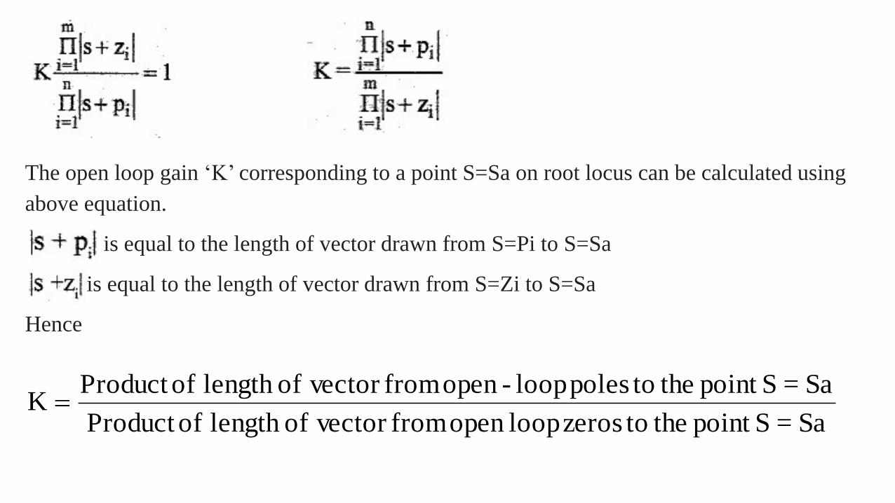
The open loop gain ‘K’ corresponding to a point S=Sa on root locus can be calculated using

above equation.

is equal to the length of vector drawn from S=Pi to S=Sa

is equal to the length of vector drawn from S=Zi to S=Sa

Hence

Sa=Spoint the tozeros loopopen from vector oflength ofProduct

Sa=Spoint the topoles loop-open from vector oflength ofProduct K

The above equation can be used to check whether a point S=Sa is a point on the root locus or

not.

<(S+Pi) is equal to the angle of vector drawn from S=Pi to S=Sa

<(S+Zi) is equal to angle of vector drawn from S=Zi to S=Sa

21212211

21

2

1

22

11

θθθrθr

θθr

r

θr

θr

rr

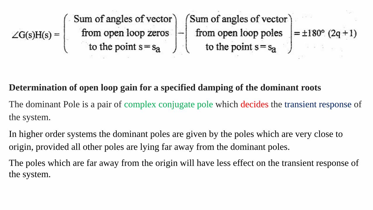
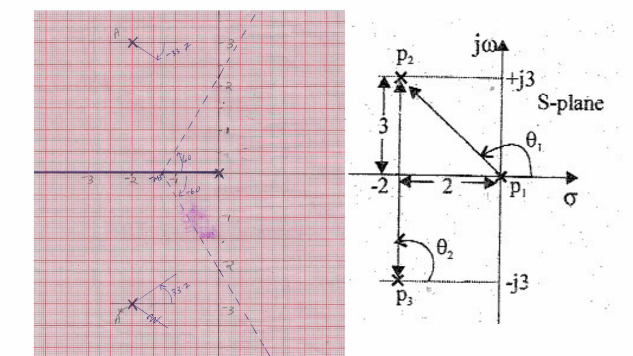
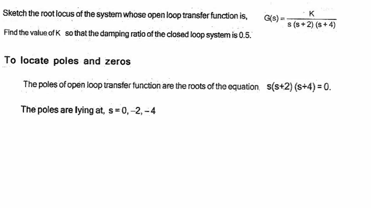
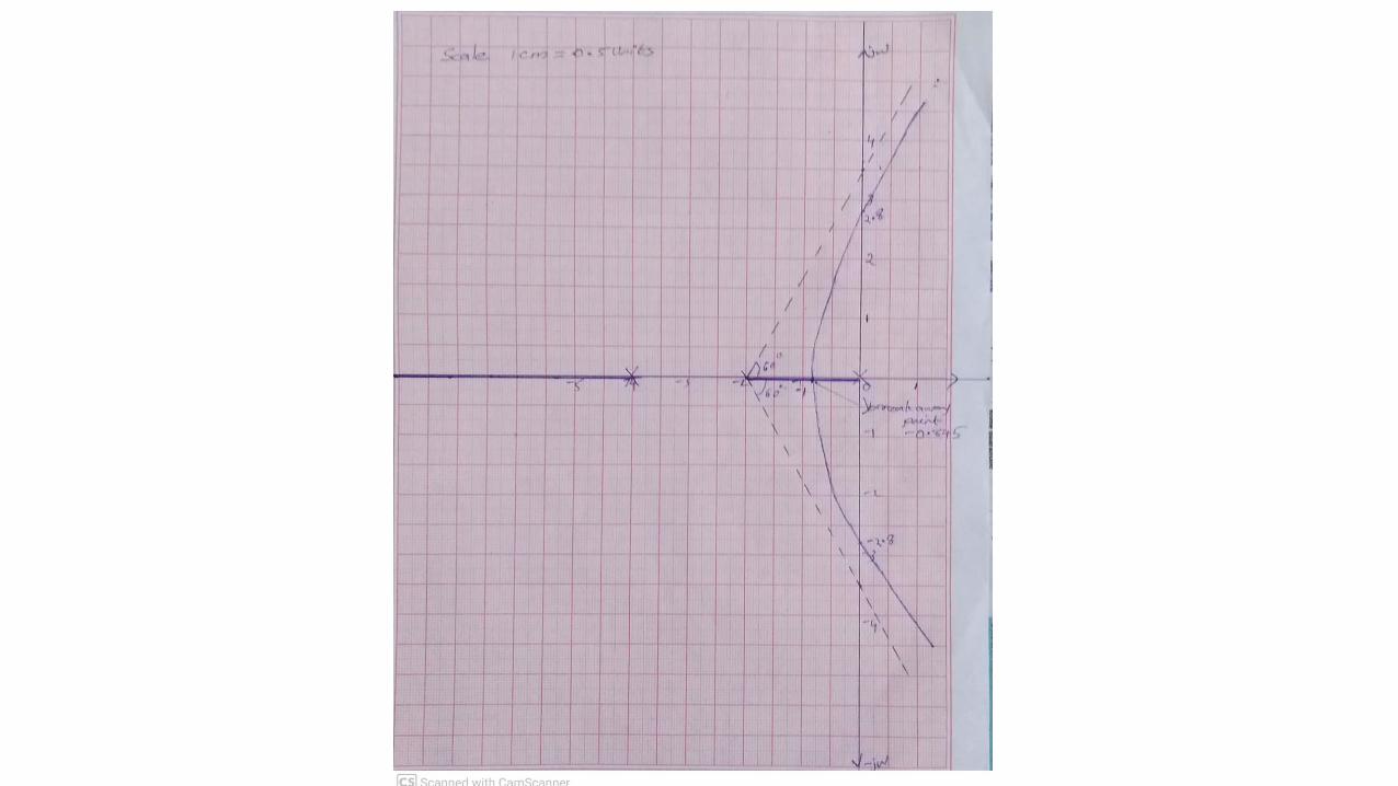
Determination of open loop gain for a specified damping of the dominant roots

The dominant Pole is a pair of complex conjugate pole which decides the transient response of

the system.

In higher order systems the dominant poles are given by the poles which are very close to

origin, provided all other poles are lying far away from the dominant poles.

The poles which are far away from the origin will have less effect on the transient response of

the system.

The transfer function of higher order system can be approximated to a second order transfer

function whose standard form of closed loop transfer function is

The dominant poles (Sd & Sd*) are given by the roots of quadratic factor

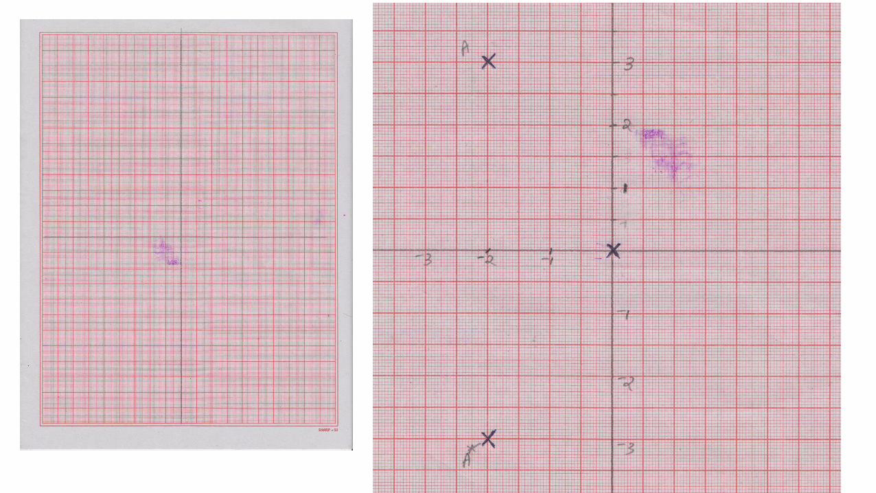
The dominant pole can be plotted on the ‘S’ plane as shown below

The dominant pole can be plotted on the ‘S’ plane as shown below

In the right angle triangle or OAP

P

A O

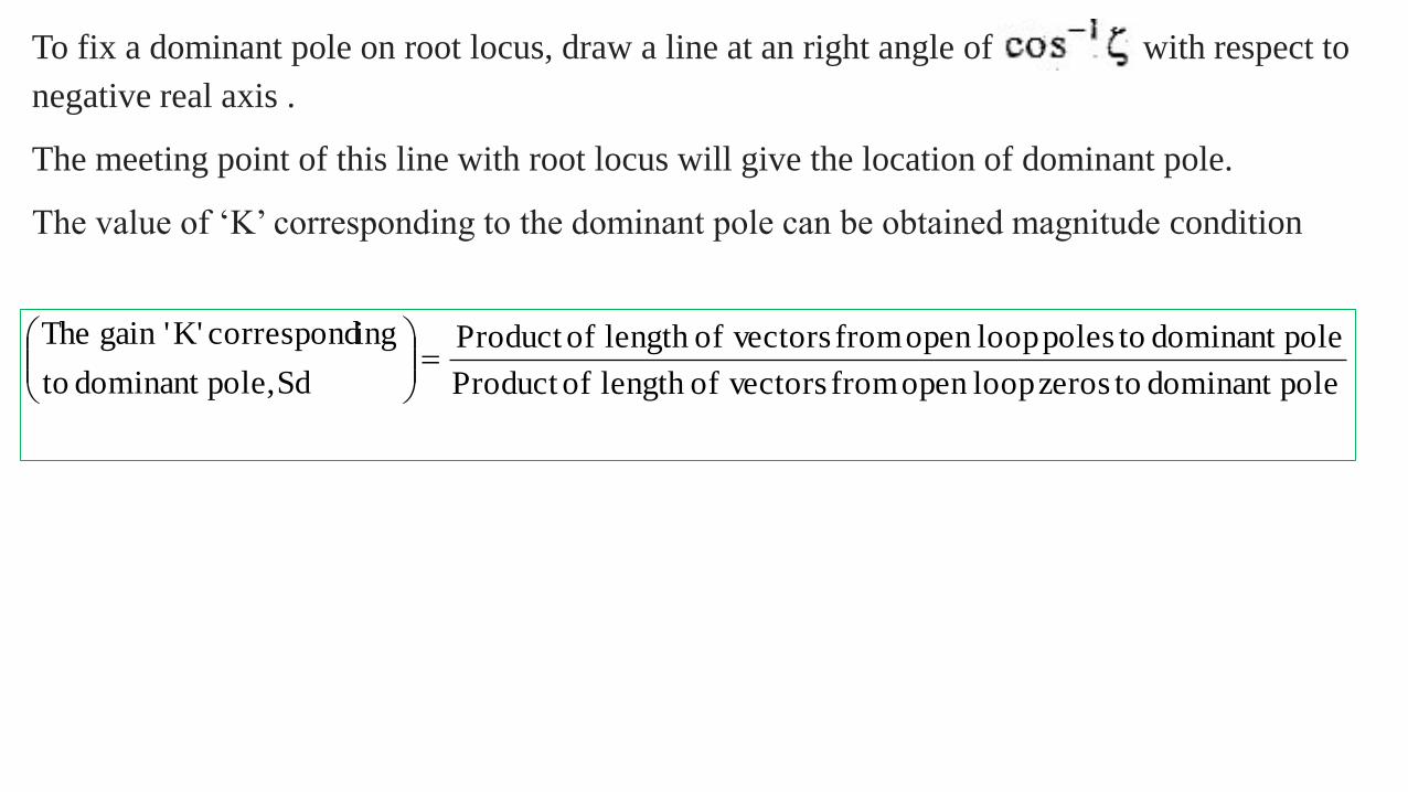
To fix a dominant pole on root locus, draw a line at an right angle of with respect to

negative real axis .

The meeting point of this line with root locus will give the location of dominant pole.

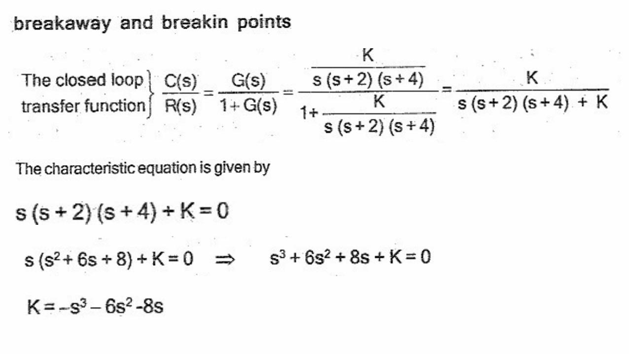
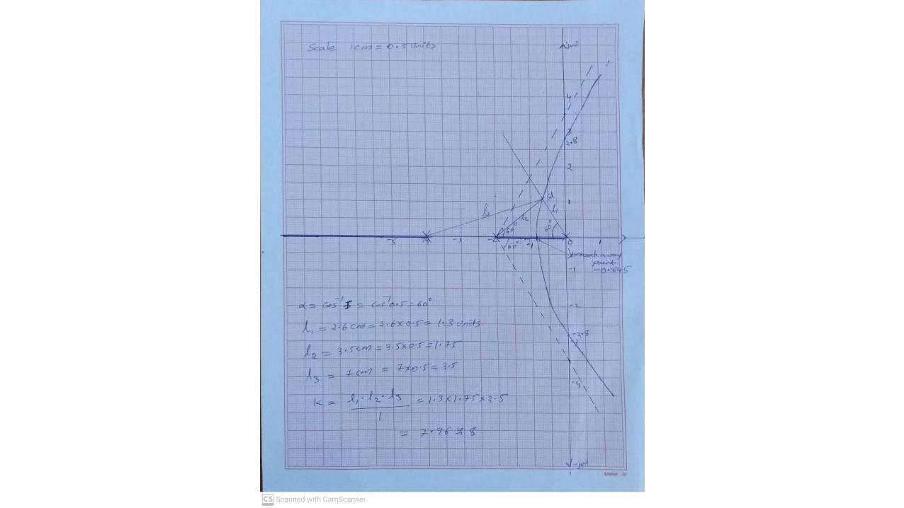
The value of ‘K’ corresponding to the dominant pole can be obtained magnitude condition

poledominant tozeros loopopen from vectorsoflength ofProduct

poledominant topoles loopopen from vectorsoflength ofProduct

Sd pole,dominant to

ingcorrespond K''gain The

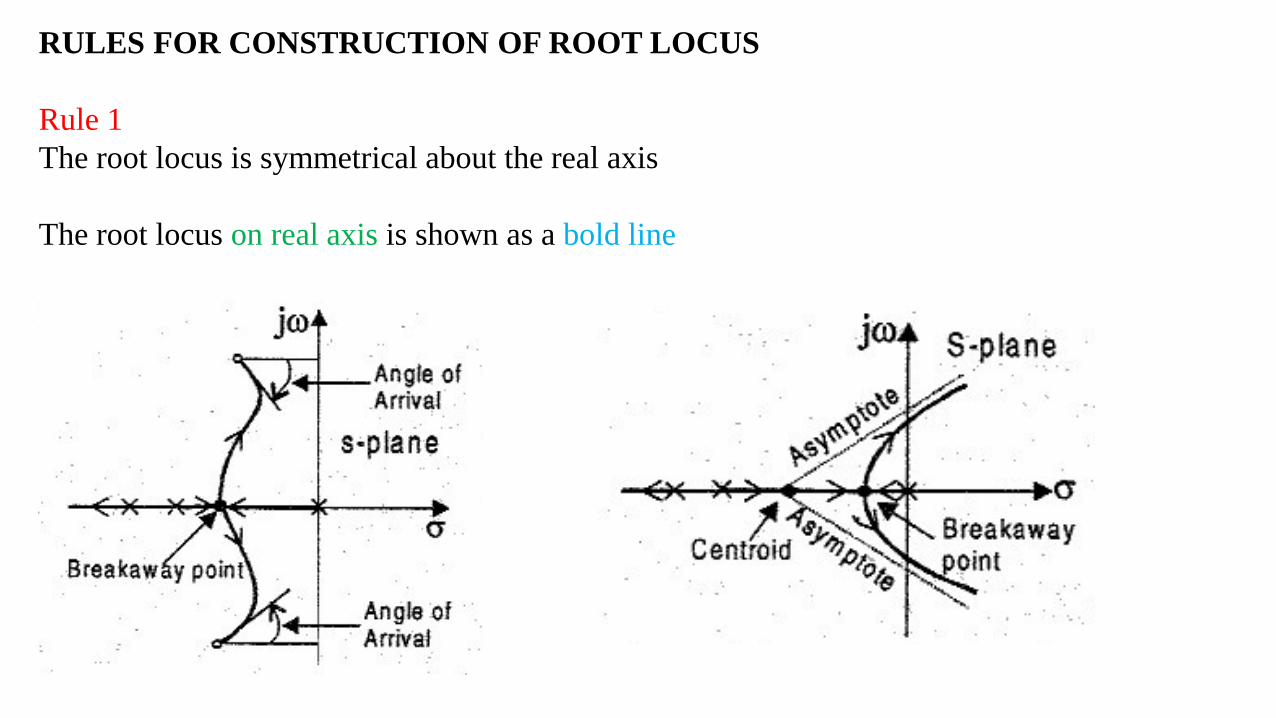
RULES FOR CONSTRUCTION OF ROOT LOCUS

Rule 1

The root locus is symmetrical about the real axis

The root locus on real axis is shown as a bold line

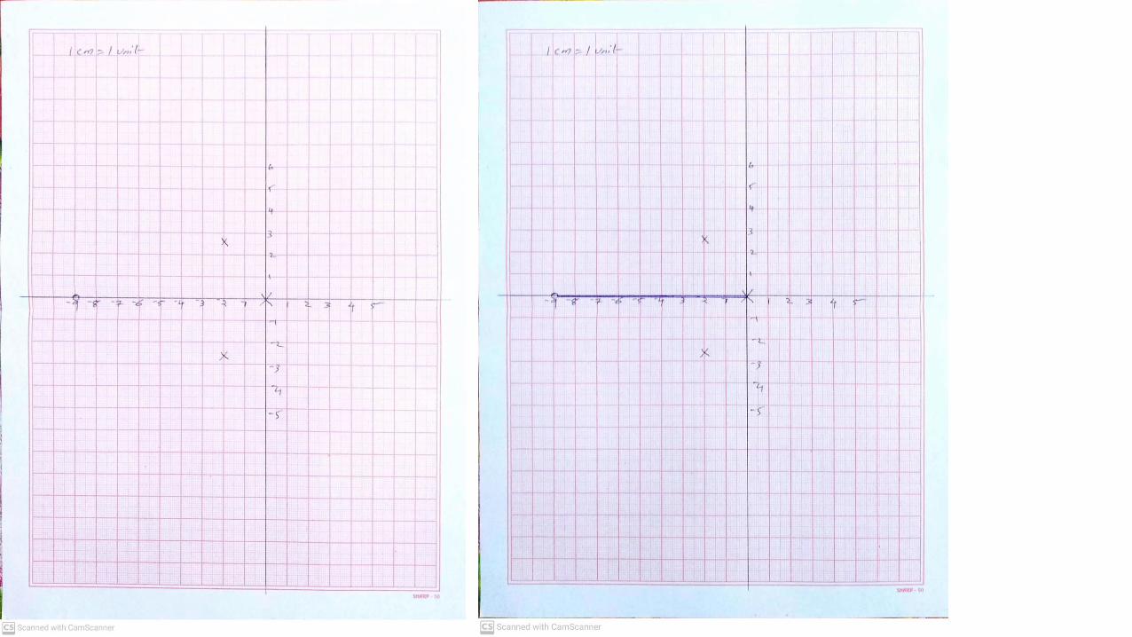
Rule 2: Location of poles and zeros

Locate the poles and zeros of G(S)H(S) on the ‘S’ plane.

The poles are marked by cross “X” and zeros are marked by small circle “o”.

The number of root locus branches is equal to number of poles of open loop transfer

function.

The root locus branch start from open loop poles and terminate at zeros.

If n=number of poles and m=number of finite zeros,

then ‘m’ root locus branches ends at finite zeros.

The remaining (n-m) root locus branches will end at zeros at infinity.

Rule 3: The root locus on real axis

To decide the part of root locus on real axis, take a test point on real axis.

If the total number of poles and zeros on the real axis to the right of this test point is odd

number then the test point lies on the root locus.

If it is even then the test point does not lie on the root locus.

The root locus on real axis is shown as a bold line

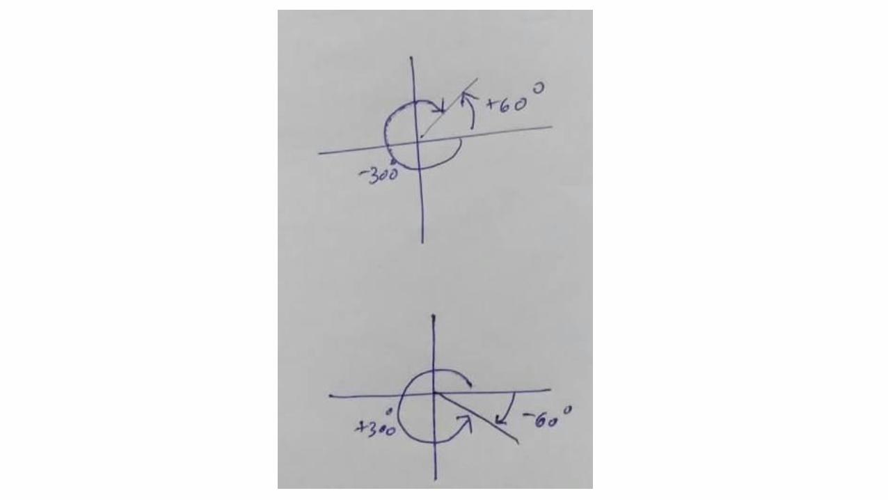
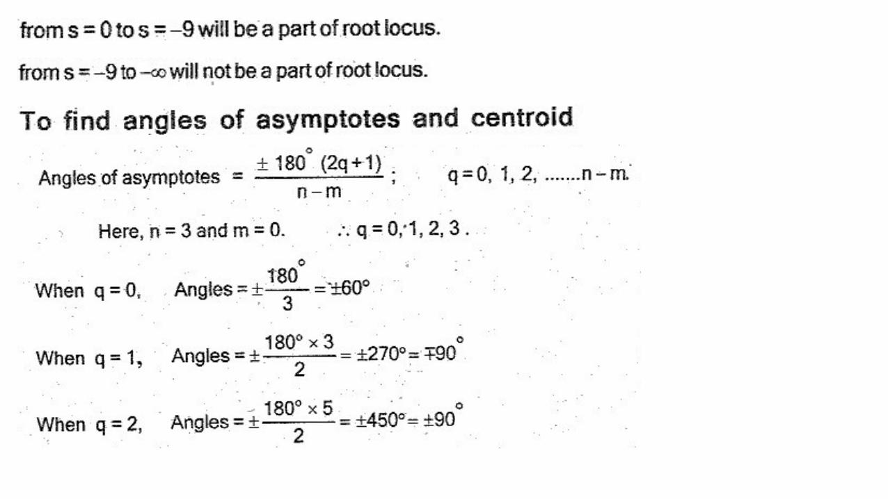
Rule 4: Angles of asymptotes and centroid

If n is number of poles and m is number of finite zeros, then n-m root locus branches will

terminate at zeros at infinity.

These n-m root locus branches will go along an asymptotic path and meets the asymptotes at

infinity.

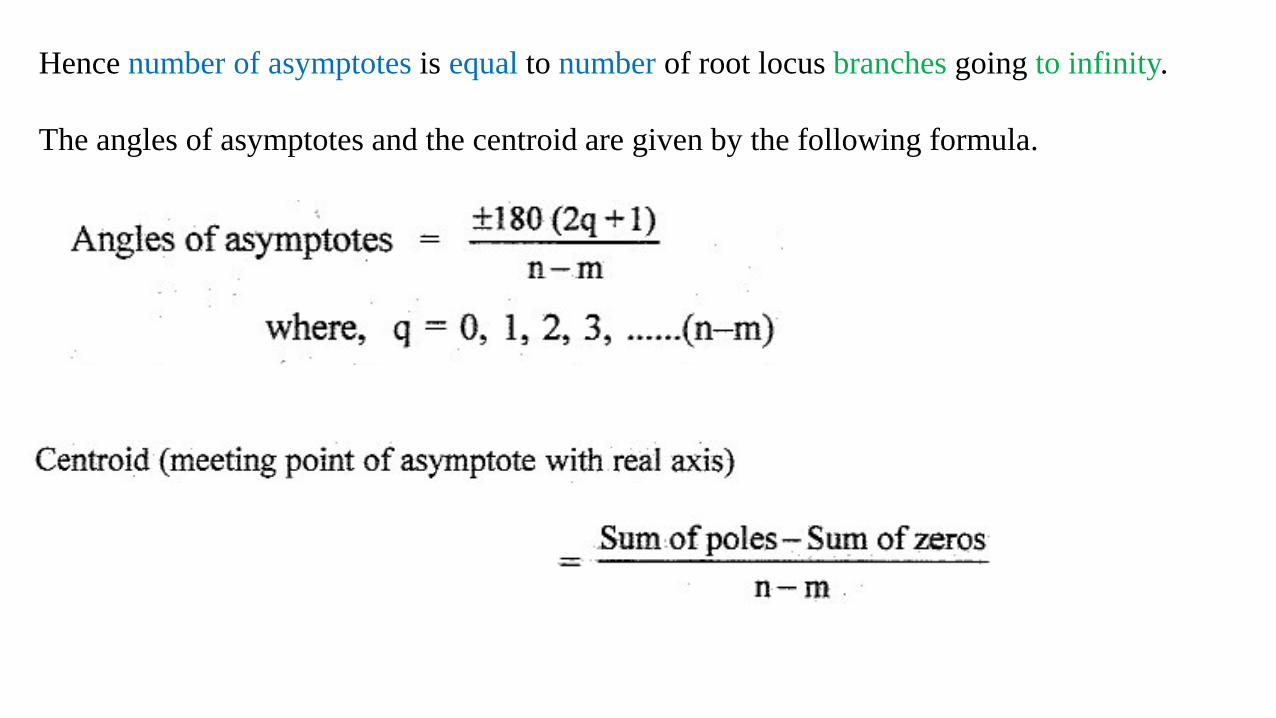
Hence number of asymptotes is equal to number of root locus branches going to infinity.

The angles of asymptotes and the centroid are given by the following formula.

Rule 5: Breakaway and Breakin points

The breakaway or breakin points either lie on real axis or exist as complex conjugate pairs.

If there is a root locus on real axis between 2 poles then there exist a breakaway point.

If there is a root locus on real axis between 2 zeros then there exist a breakin point.

Let the C.E. be in the form

The breakaway and breakin point is given by roots of the equation

Substitute the value of ‘S’ in equation -1

If the gain ‘K’ is positive and real, then there exist a breakaway or breakin point

0dS

dK

1

Rule 5: Breakaway and Breakin points

The breakaway or breakin points either lie on real axis or exist as complex conjugate pairs.

If there is a root locus on real axis between 2 poles then there exist a breakaway point.

If there is a root locus on real axis between 2 zeros then there exist a breakin point.

Let the C.E. be in the form

The breakaway and breakin point is given by roots of the equation

Substitute the value of ‘S’ in equation -1

If the gain ‘K’ is positive and real, then there exist a breakaway or breakin point

0dS

dK

1

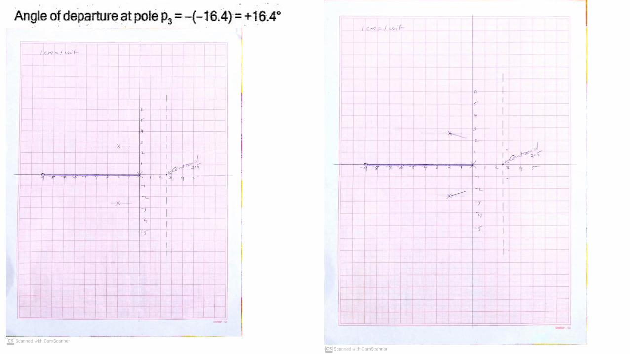
Rule 6: Angle of Departure and angle of arrival

zeros fromA polecomplex theto

vectorsof angles of sum

polesother fromA polecomplex theto

vector of angles of sum180

A polecomplex a from

departure of Angle0

poles fromA zerocomplex theto

vectorsof angles of sum

zerosother all fromA zerocomplex theto

vectorsof angles of sum180

A zerocomplex aat

arrival of Angle0

Rule 7: Point of intersection of root locus with imaginary axis

Letting s =j in the C.E and separate the real part and imaginary part.

Equate real part to zero.

Equate imaginary part to zero.

Solve the equation for w and K.

The value of ‘ ’ gives the point where the root locus crosses imaginary axis.

The value of K gives the value of gain K at the crossing point.

This value of K is the limiting value of K for stability of the system

ω

ω

Rule 8: Test points and root locus

Take a series of test point in the broad neighbourhood of the origin of the ‘S’ plane and adjust

the test point to satisfy angle criterion.

Sketch the root locus by joining the test point by smooth curve

There is no root locus exist between two poles or two zeros. So the root locus has neither

breakaway nor breakin point

ANGLE OF DEPARTURE OR ANGLE OF ARRIVAL

Since there is no complex pole or complex zero, there will be no angle of departure or angle

of arrival

EFFECT OF ADDITION OF POLES AND ZEROS ON ROOT LOCUS

Consider

The root locus is

now add one pole at S= --5

The corresponding root locus is given by

4)S(S

KG(S)H(S)

5)4)(sS(S

KG(S)H(S)

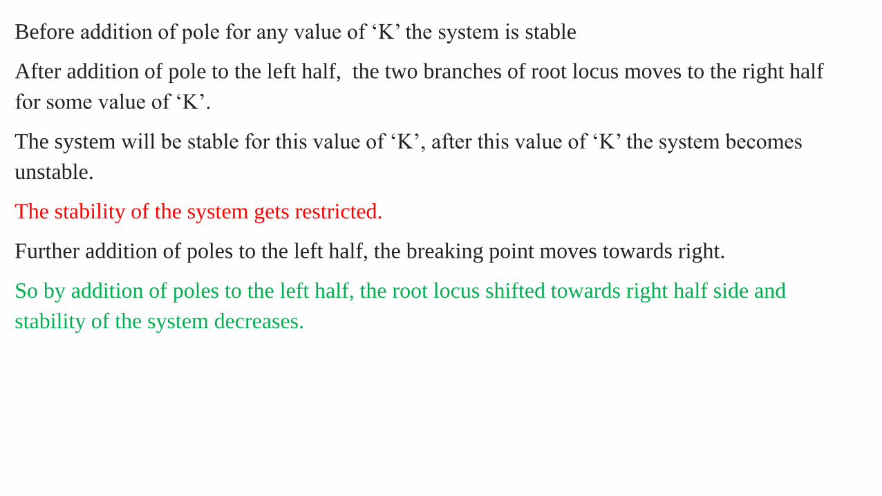
Before addition of pole for any value of ‘K’ the system is stable

After addition of pole to the left half, the two branches of root locus moves to the right half

for some value of ‘K’.

The system will be stable for this value of ‘K’, after this value of ‘K’ the system becomes

unstable.

The stability of the system gets restricted.

Further addition of poles to the left half, the breaking point moves towards right.

So by addition of poles to the left half, the root locus shifted towards right half side and

stability of the system decreases.

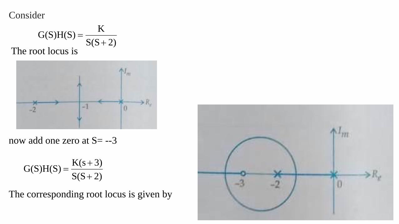
Consider

The root locus is

now add one zero at S= --3

The corresponding root locus is given by

2)S(S

KG(S)H(S)

2)S(S

3)K(sG(S)H(S)

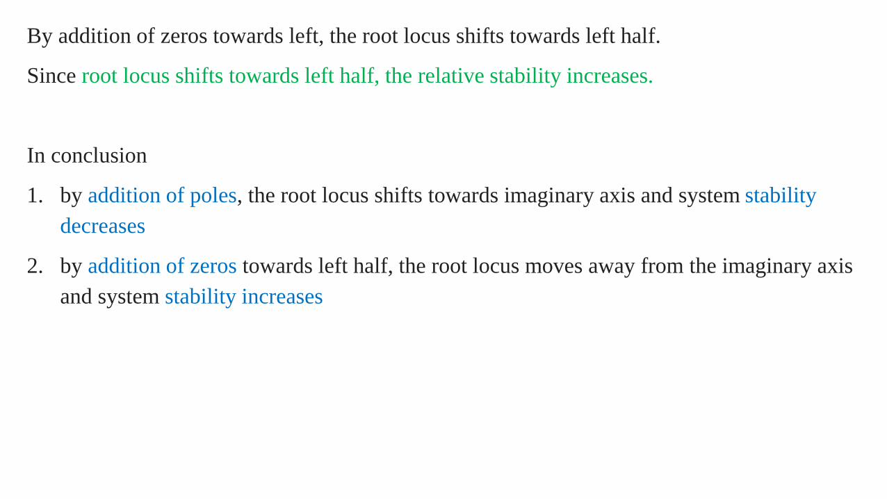
By addition of zeros towards left, the root locus shifts towards left half.

Since root locus shifts towards left half, the relative stability increases.

In conclusion

1. by addition of poles, the root locus shifts towards imaginary axis and system stability

decreases

2. by addition of zeros towards left half, the root locus moves away from the imaginary axis

and system stability increases

MODULE V

FREQUENCY DOMAIN ANALYSIS

Frequency domain specifications

Bode plot

Log magnitude vs. phase plot,

FREQUENCY DOMAIN ANALYSIS

Frequency response is the steady state response of a system when the input

to the system is a sinusoidal signal.

Consider a LTI system

let r(t) be an input sinusoidal signal.

The response or output y(t) is also a sinusoidal signal of the same frequency

but with different magnitude and phase angle.

The magnitude and phase relationship between the sinusoidal input and the steady state output

of the system is termed as frequency response.

In the system transfer function T(S), if ‘S’ is replaced by j-Omega ( )

then the resulting transfer function T( ) is called sinusoidal transfer function.

The frequency response of the system can be directly obtained from the sinusoidal transfer

function T( ) of the system.

jω

jω

jω

The advantage of frequency response analysis

The absolute and relative stability of the closed loop system can be estimated from the

knowledge of their open loop frequency response.

The practical testing of the system can be easily carried with available sinusoidal signal

generators and precise measurement equipment

The transfer function of complicated systems can be determined experimentally by frequency

response tests.

The design and parameter adjustment of the open loop transfer function of a system for

specified closed-loop performance is carried out more easily in frequency domain.

When the system is designed by use of the frequency response analysis the effect of noise

disturbances and parameters variations are relatively easy to visualise and incorporate

corrective measures.

The frequency response analysis and response can be extended to certain nonlinear control

systems.

Frequency domain specifications

1. resonant peak Mr

2. resonant frequency

3. bandwidth

4. cutoff rate

5. gain margin

6. phase margin

Resonant peak

The maximum value of the magnitude of closed loop transfer function is called resonant peak

(Mr)

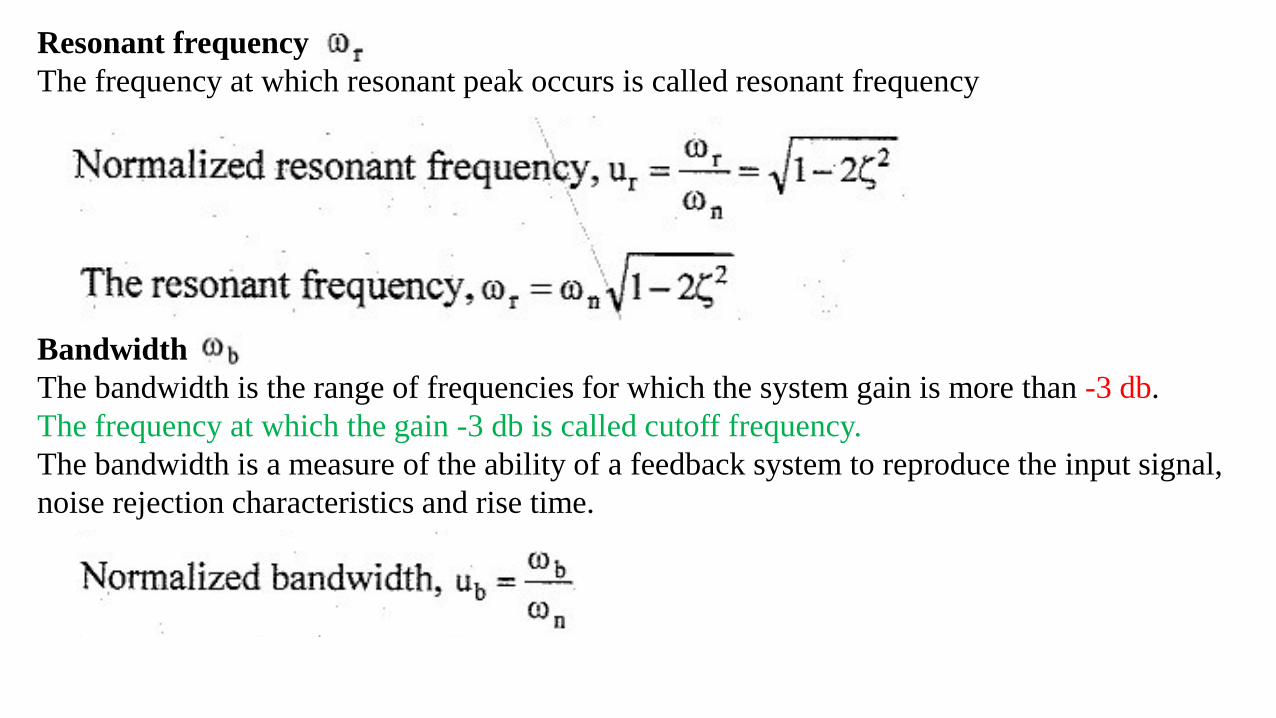
Resonant frequency

The frequency at which resonant peak occurs is called resonant frequency

Bandwidth

The bandwidth is the range of frequencies for which the system gain is more than -3 db.

The frequency at which the gain -3 db is called cutoff frequency.

The bandwidth is a measure of the ability of a feedback system to reproduce the input signal,

noise rejection characteristics and rise time.

Cut off rate

The slope of the log magnitude curve near the cutoff frequency is called the cutoff rate.

The cut off rate indicates the ability of the system to distinguish the signal from the noise.

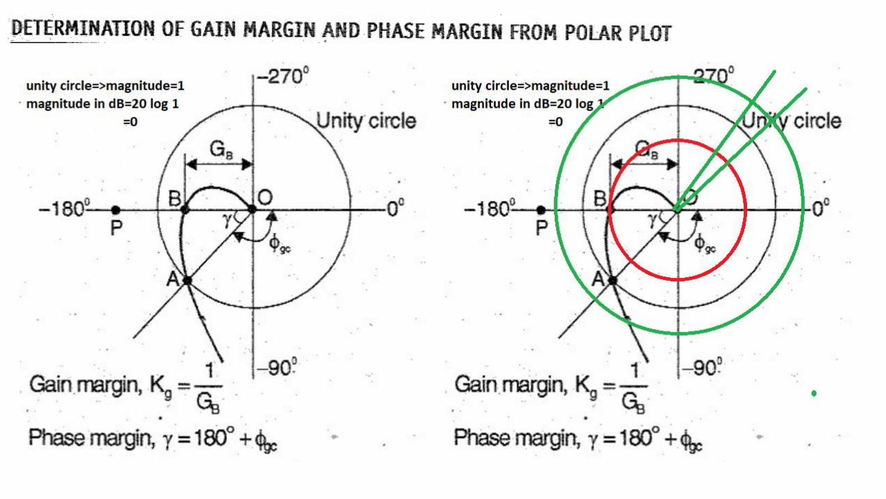
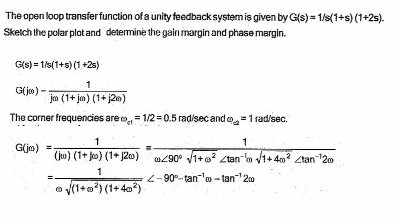
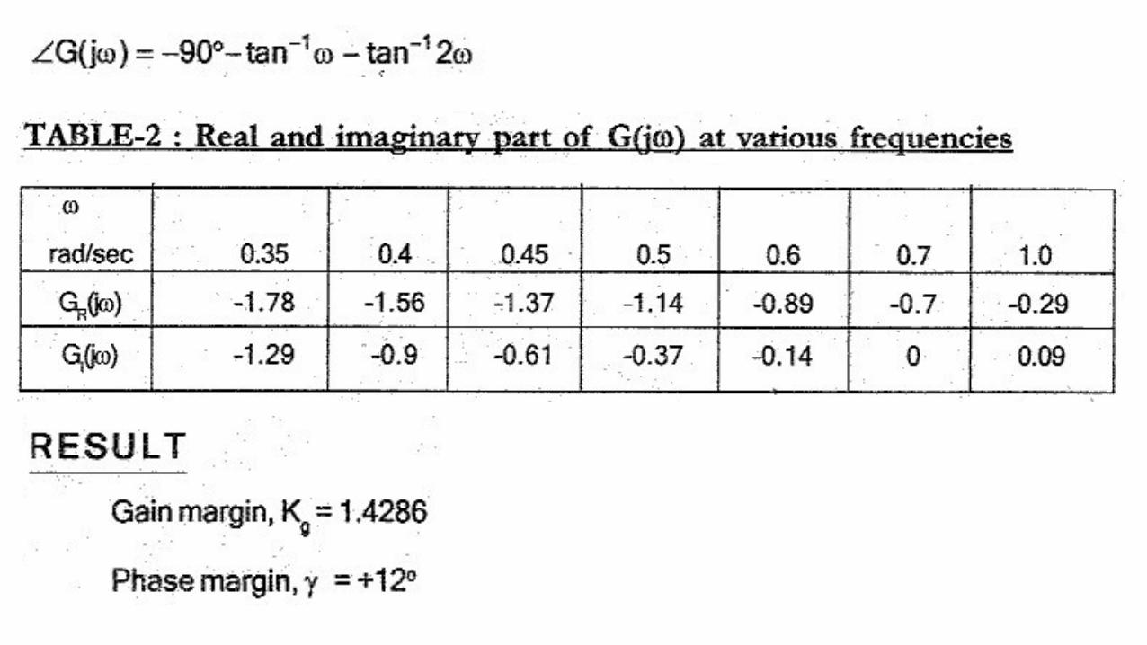
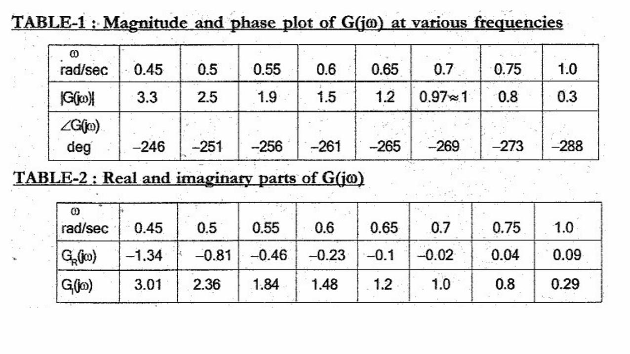
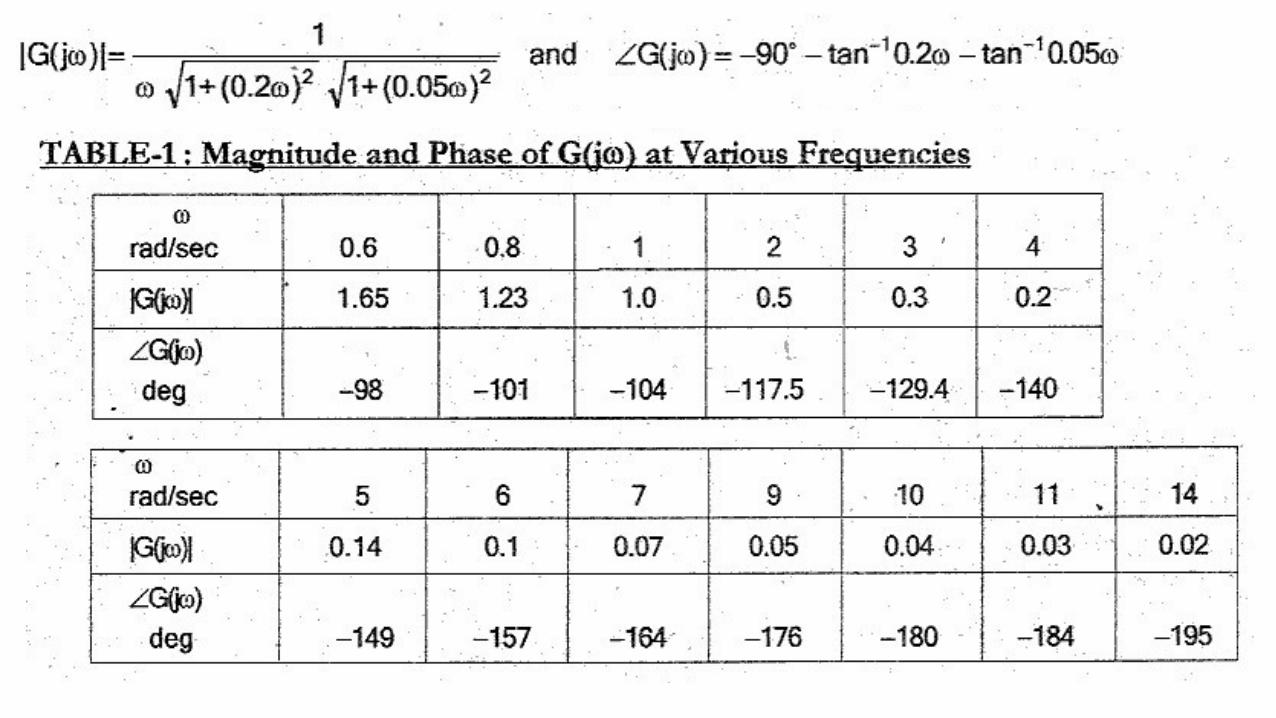
Gain margin kg

The gain margin kg is defined as the reciprocal of the magnitude of open loop transfer function

at phase crossover frequency.

The frequency at which the phase of open loop transfer function is ‘- 180 degree’ is called the

phase crossover frequency

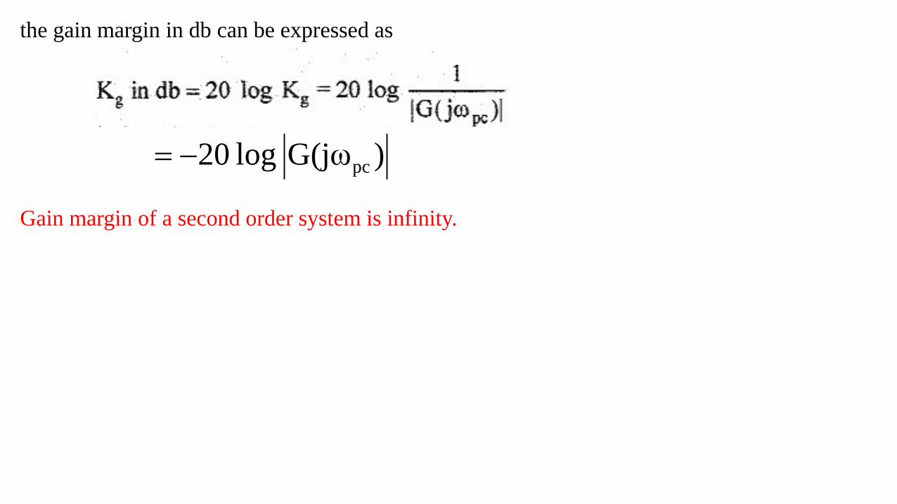
the gain margin in db can be expressed as

Gain margin of a second order system is infinity.

)G(jω log 20 pc

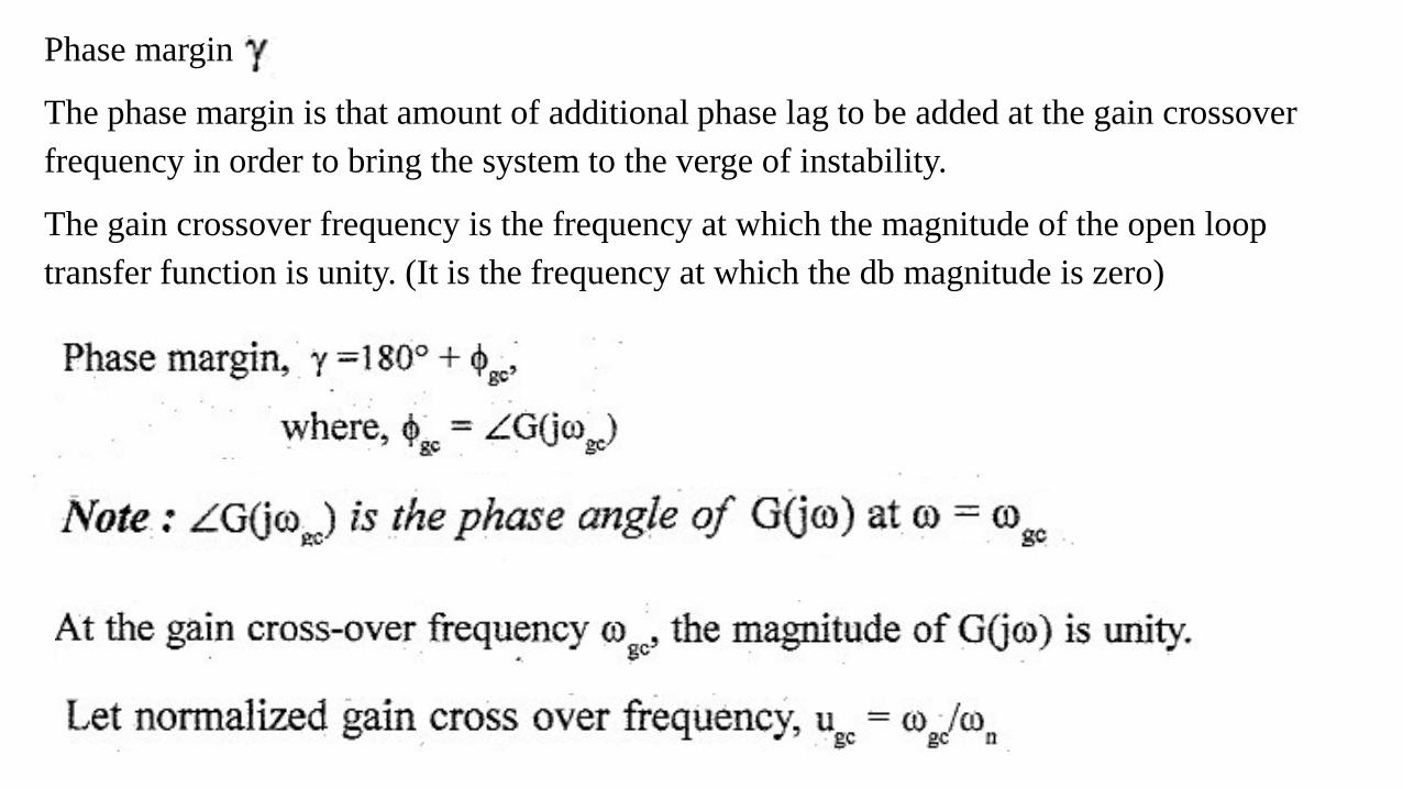
Phase margin

The phase margin is that amount of additional phase lag to be added at the gain crossover

frequency in order to bring the system to the verge of instability.

The gain crossover frequency is the frequency at which the magnitude of the open loop

transfer function is unity. (It is the frequency at which the db magnitude is zero)

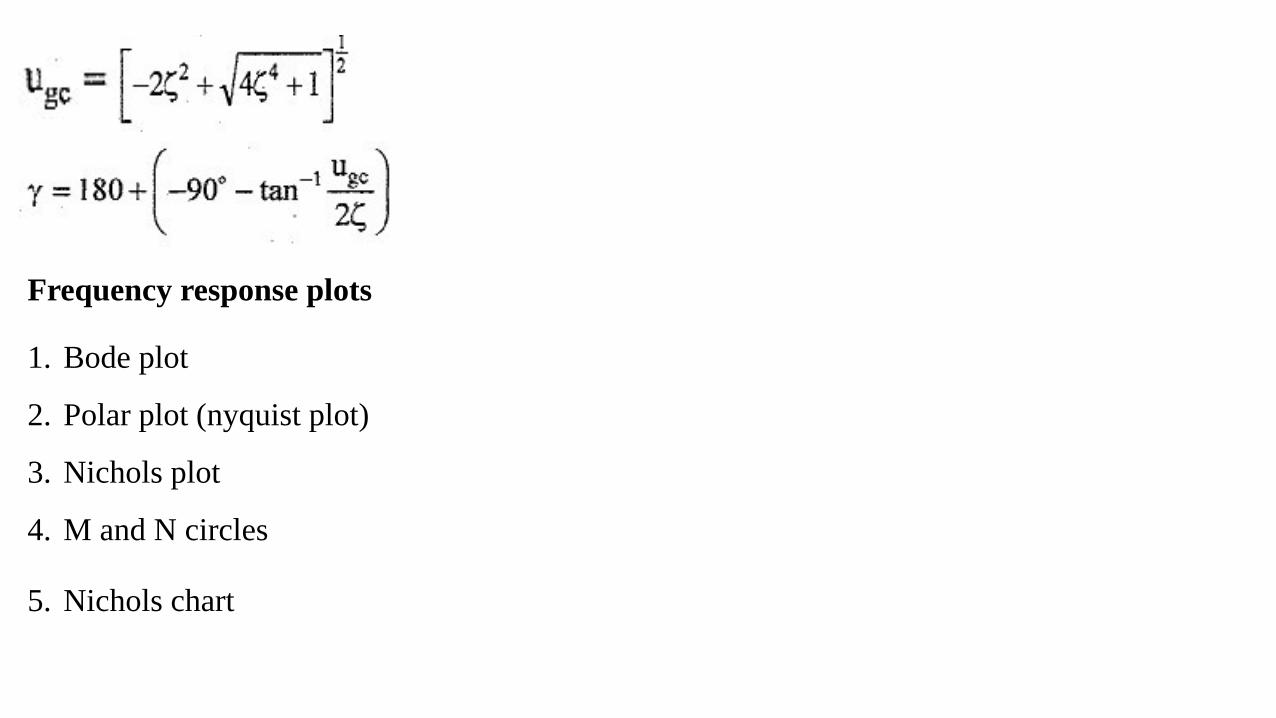
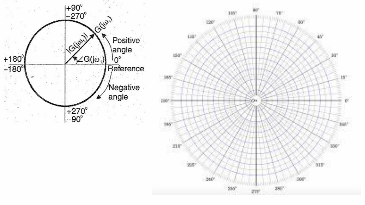
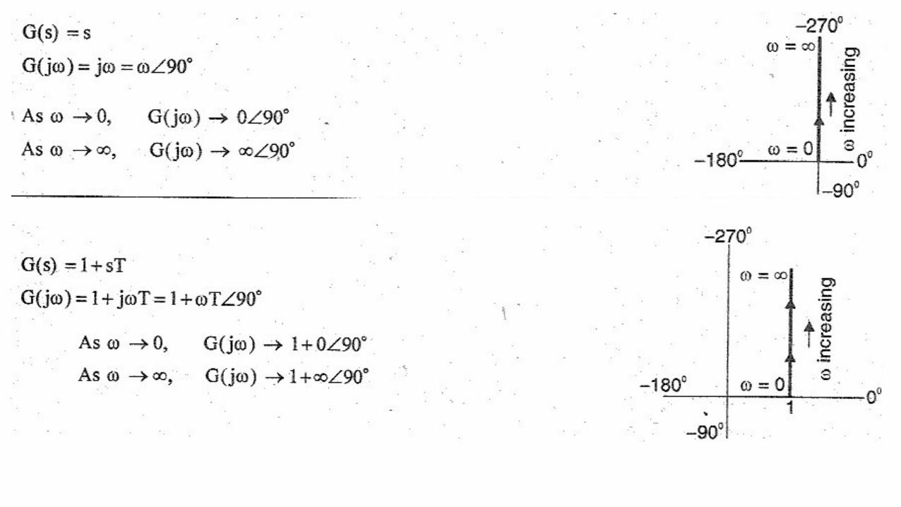
Frequency response plots

1. Bode plot

2. Polar plot (nyquist plot)

3. Nichols plot

4. M and N circles

5. Nichols chart

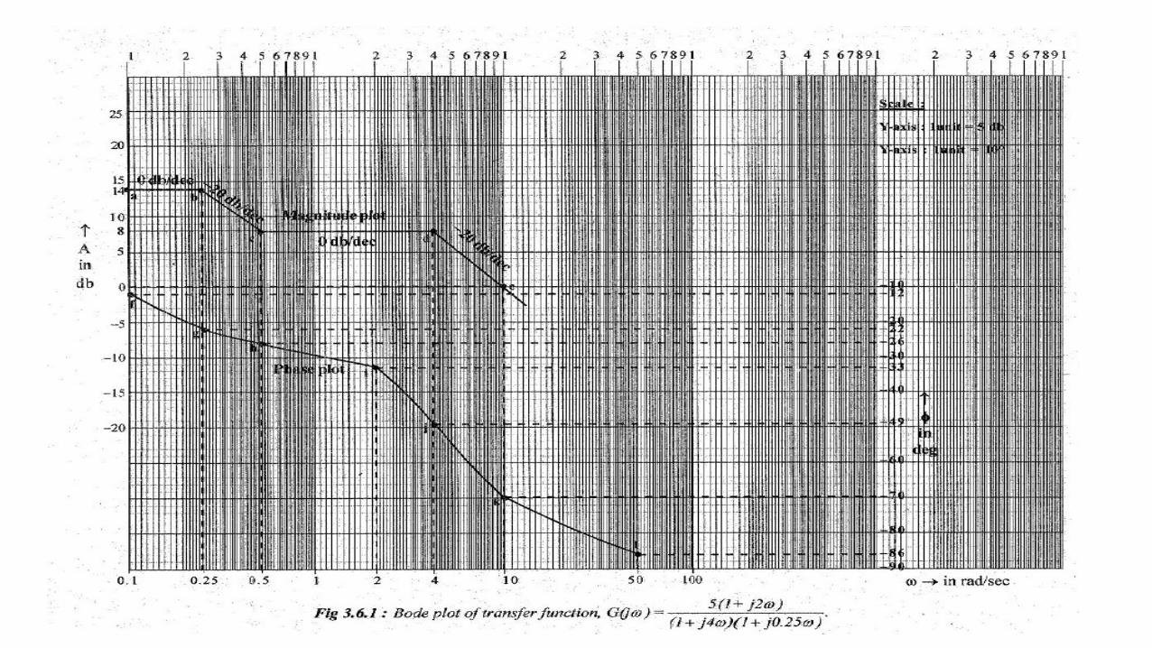
Bode plot

A bode plot consist of two graph

One is a product of the magnitude of a sinusoidal transfer function versus log Omega ( )

The other is a plot of the phase angle of a sinusoidal transfer function versus log Omega ( )

The bode plot can be drawn for both open loop and closed loop transfer function

Usually the bode plot is drawn for open loop system.

ω log

ω log

When the magnitude is expressed in db, the multiplication is converted to addition.

In magnitude plot, the db magnitudes of individual factors of can be added.

Individual factors of

1. constant gain

2. integral factor

3. derivative factor

4. first order factor in denominator

5. first order factor in numerator

6. quadratic factor in denominator

7. quadratic factor in numerator

)( jG

)( jG

1. constant gain

2. integral factor

3. derivative factor

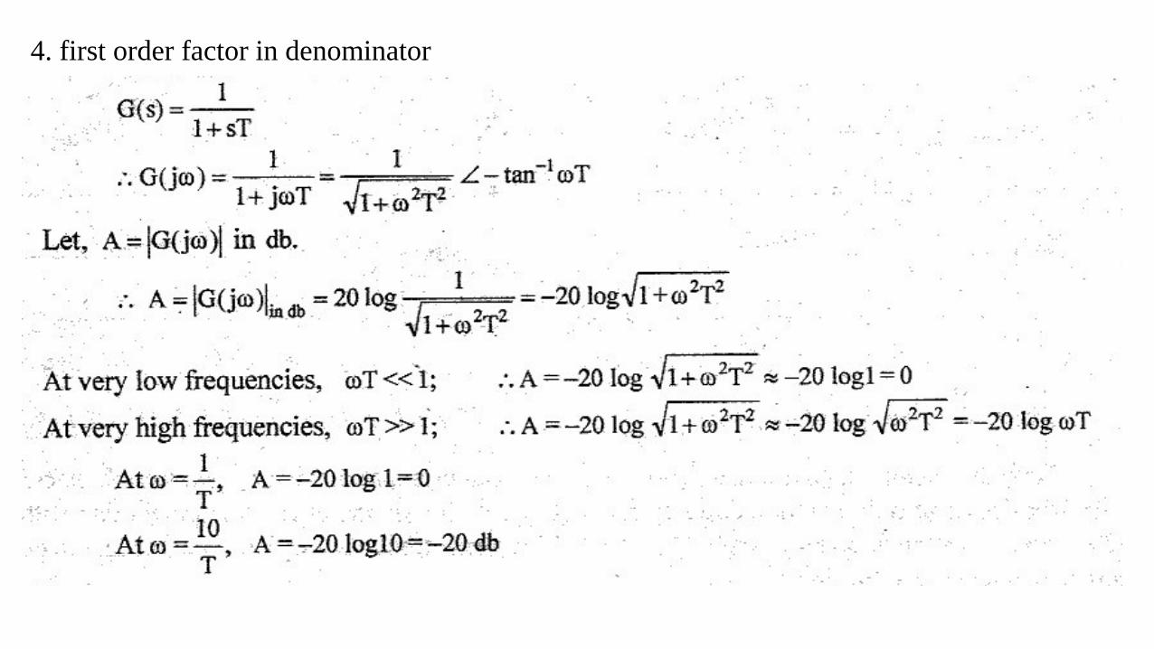
4. first order factor in denominator

Magnitude plot can be approximated by two straight line

One is a straight line at 0db for the frequency range

Second one is a straight line with slope –20 db/dec for the frequency range,

The two straight lines are asymptotes of the exact curve.

The frequency at which the two asymptotes meet is called corner frequency or break

frequency

For factor the frequency is the corner frequency

It divides the frequency response curve into two region, a curve for low frequency region and

a curve for high frequency region

The actual magnitude at the corner frequency, is,

5. first order factor in numerator

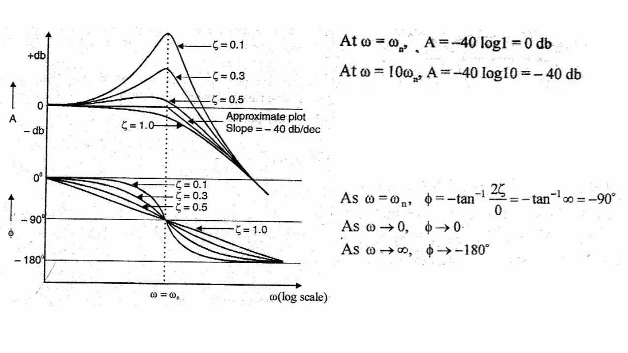
6. quadratic factor in denominator

Magnitude plot can be approximated by two straight line

One is a straight line at 0db for the frequency range

Second one is a straight line with slope –40 db/dec for the frequency range,

The two straight lines are asymptotes of the exact curve.

The frequency at which the two asymptotes meet is called corner frequency or break

frequency

For quadratic factor the frequency is the corner frequency

7. quadratic factor in numerator

Magnitude plot can be approximated by two

straight line

One is a straight line at 0db for the frequency

range

Second one is a straight line with slope +40

db/dec for the frequency range,

The two straight lines are asymptotes of the

exact curve.

For quadratic factor is the corner frequency

40 x

y1- tan

ω

jω

ω

ωj2ξ1 7.

40- x

y1-tan-

ω

jω

ω

ωj2ξ1

1 6.

20m ωT tanm Tj1 5.

20m- ωT tanm- Tj1

1 4.

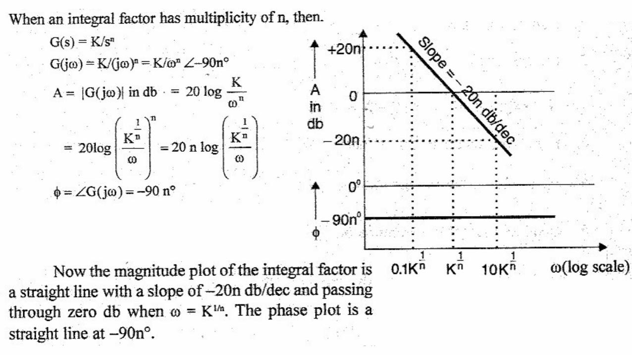
n20 90n jωK 3.

n20- 90n - jω

K 2.

0 0 K 1.

Slope Angle factors Individual

2

n

2

nn

1-m

1-

m

n

n

n

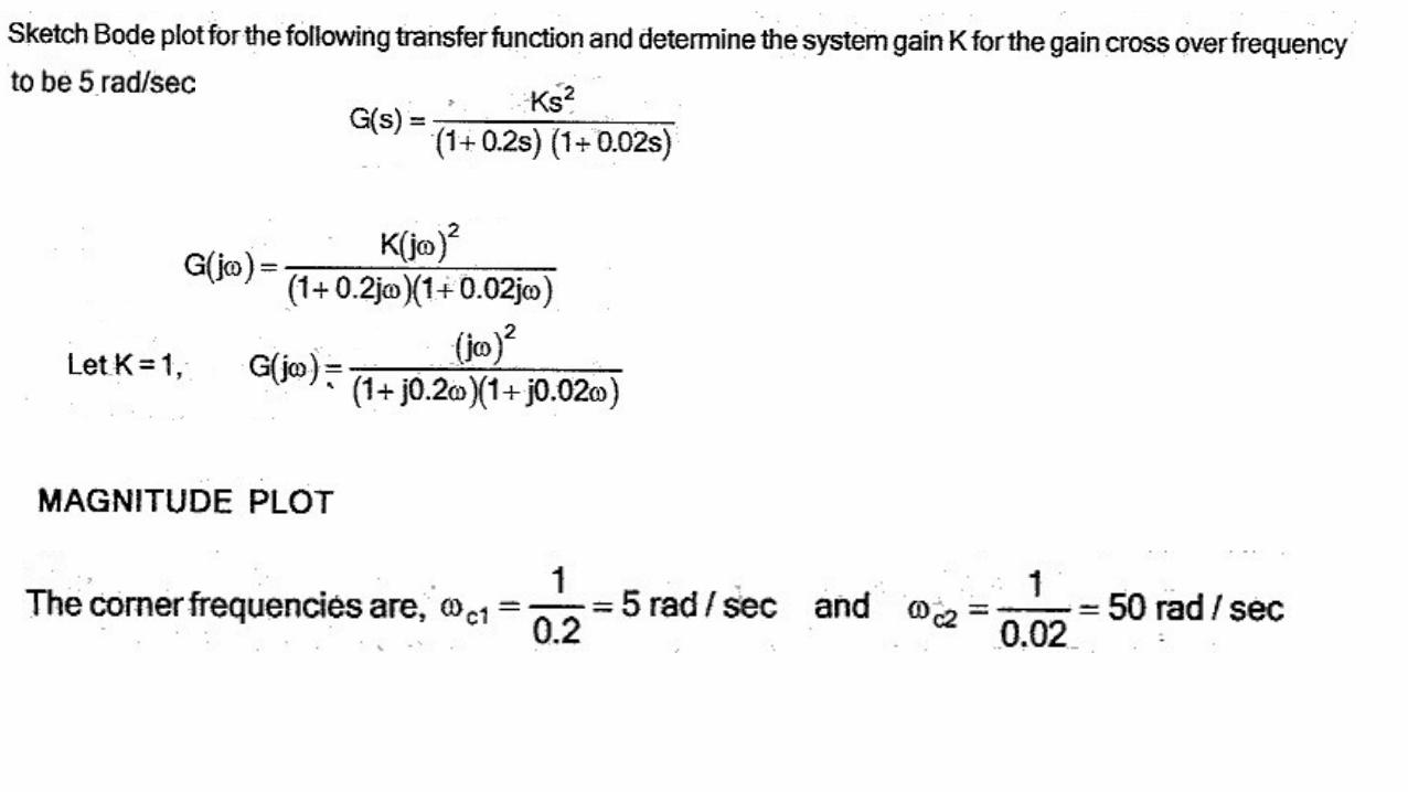
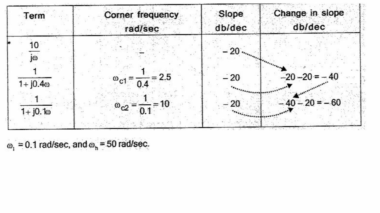
BODE PLOT

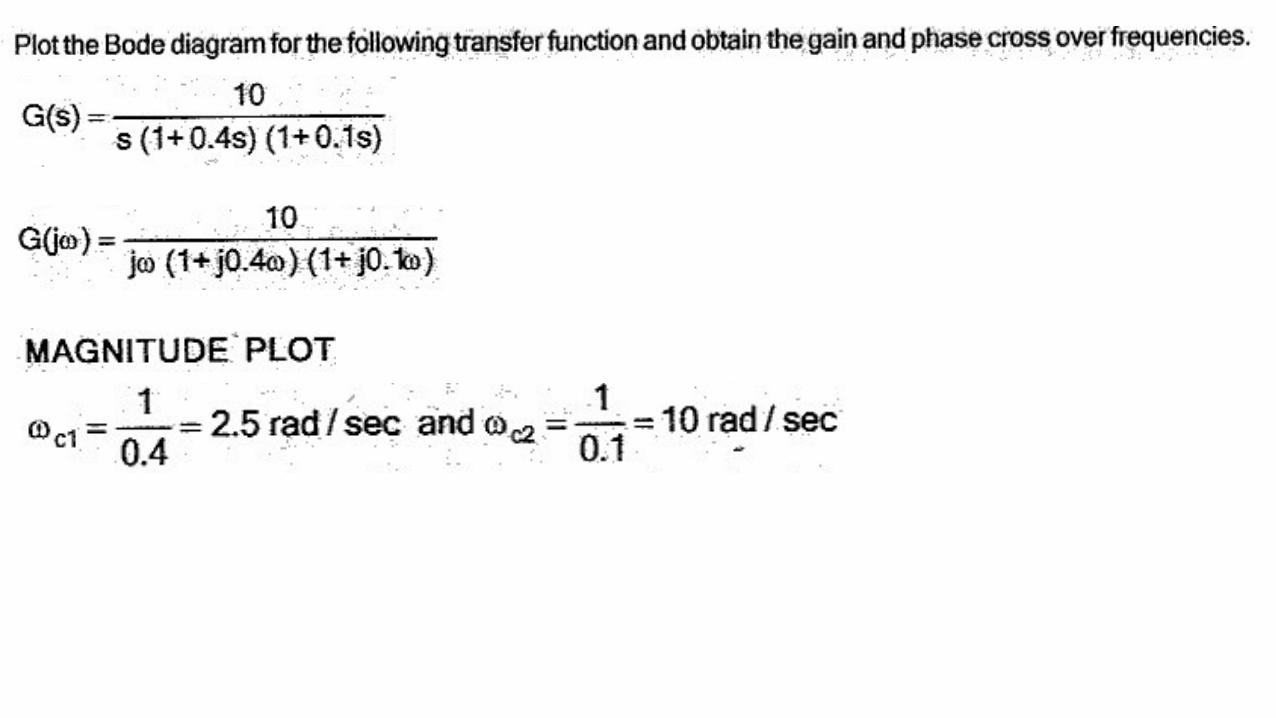
Procedure for plotting magnitude plot

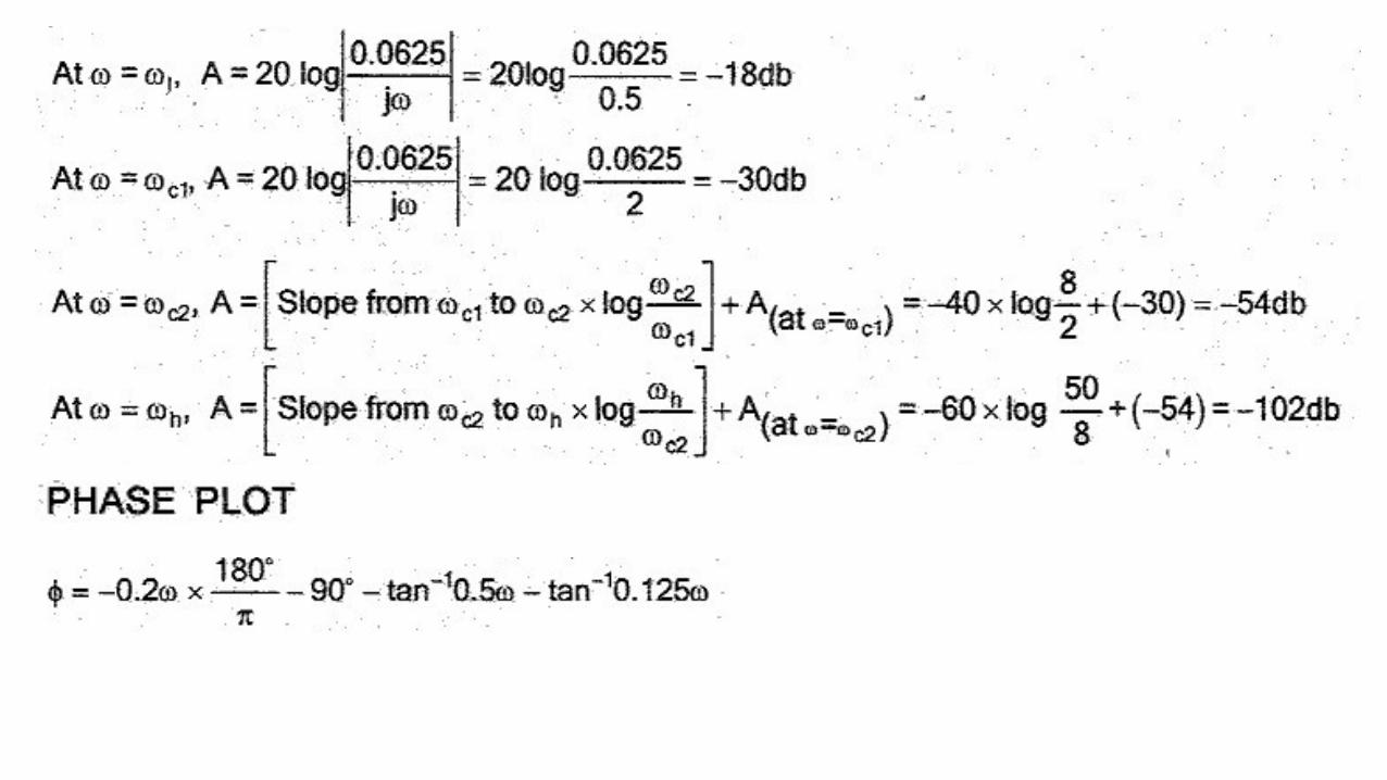
1. Put in open loop TF

2. Find corner frequencies

list the corner frequencies in the increasing order and prepare a table as shown below

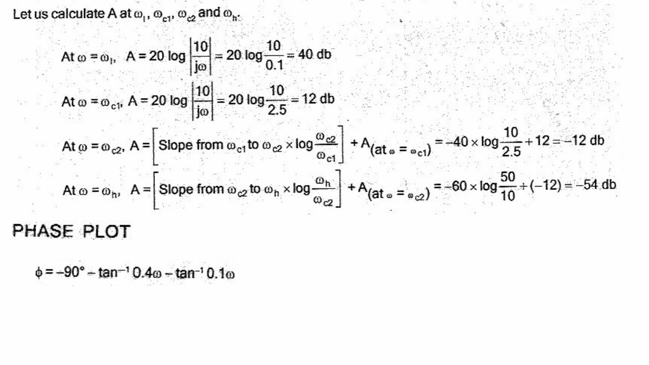
3. find Lower frequency and higher frequencies

calculate the db magnitude of and at the lowest corner frequency

jS

chcl ωω and ωω

ωlat jωK ,

jω

K K,

n

n

T

1ω T),j(1for c

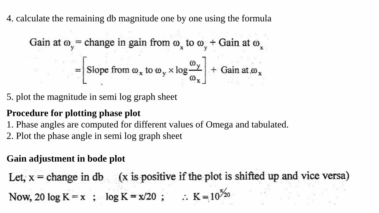
4. calculate the remaining db magnitude one by one using the formula

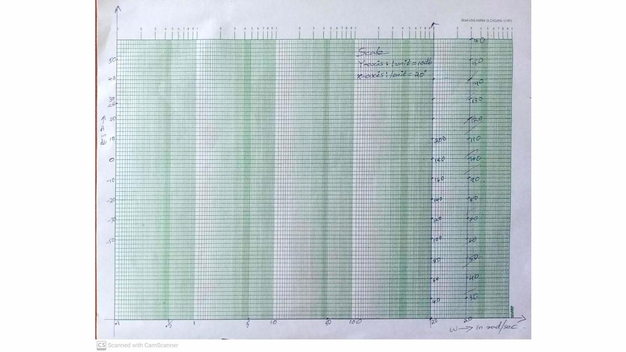
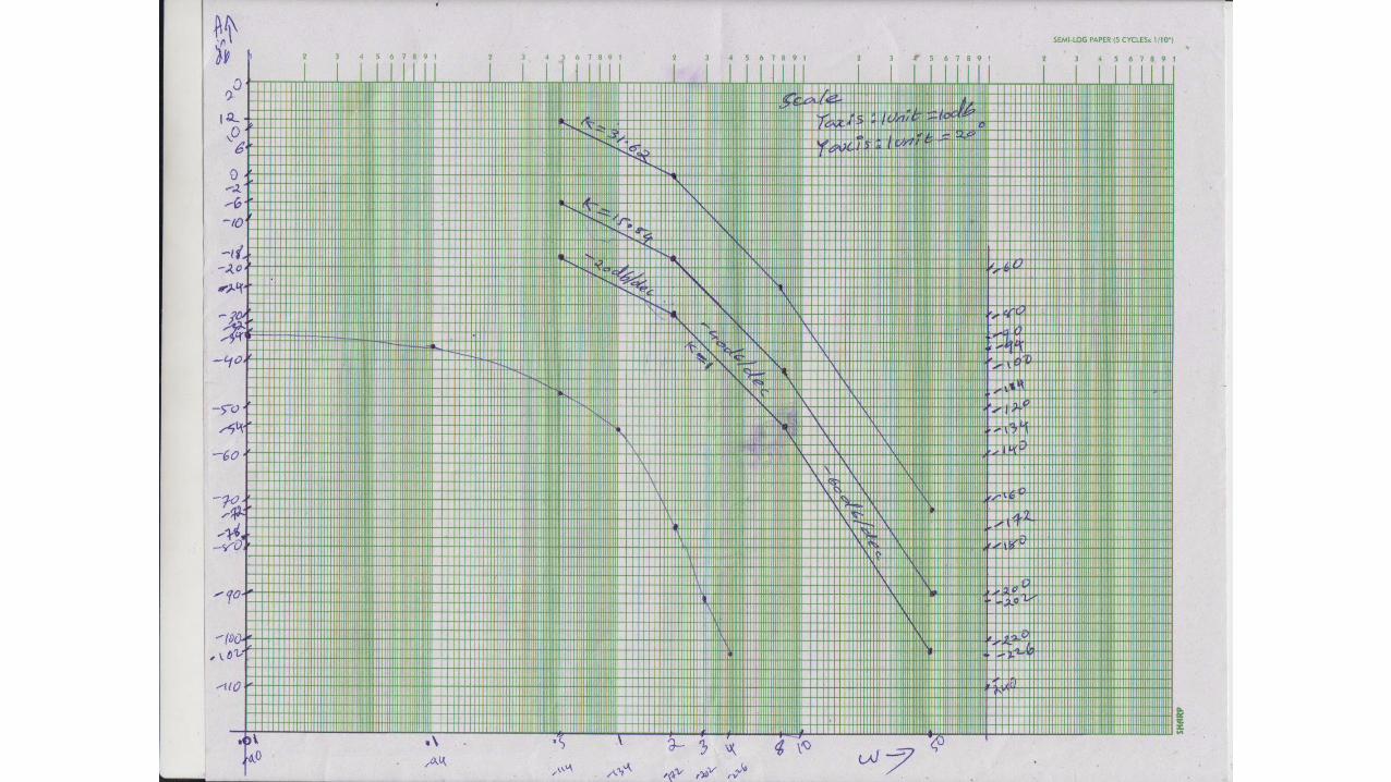
5. plot the magnitude in semi log graph sheet

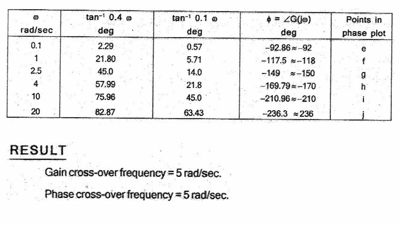
Procedure for plotting phase plot

1. Phase angles are computed for different values of Omega and tabulated.

2. Plot the phase angle in semi log graph sheet

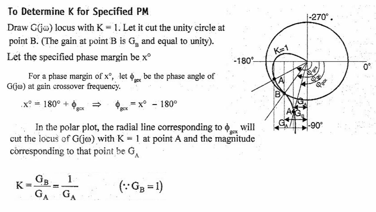
Gain adjustment in bode plot

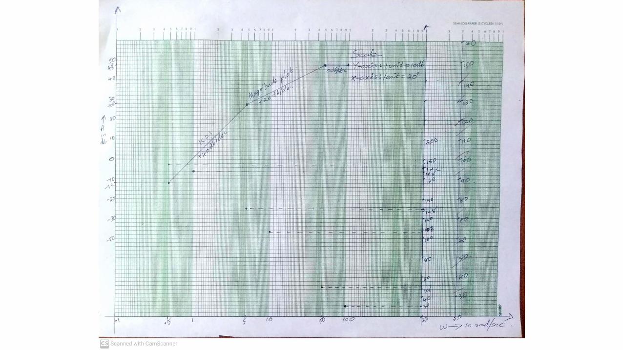
Given that gain cross over frequency is 5rad/sec

At w=5rad/sec the gain is 28db.

If gain crossover frequency is 5rad/sec then at that frequency the db gain should be zero.

Hence to every point of magnitude plot a db gain of -28db should be added.

The addition of -28db shifts the plot downwards.

The magnitude correction is independent of frequency.

For quadratic factor the frequency is the corner frequency

chcl ωω and ωω find Lower frequency and higher frequencies

rsinθb rcosθa

a

btanθ b2a2r

reθriba

1

iθ

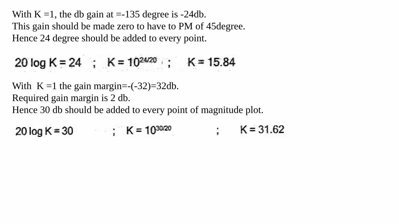
With K =1, the db gain at =-135 degree is -24db.

This gain should be made zero to have to PM of 45degree.

Hence 24 degree should be added to every point.

With K =1 the gain margin=-(-32)=32db.

Required gain margin is 2 db.

Hence 30 db should be added to every point of magnitude plot.

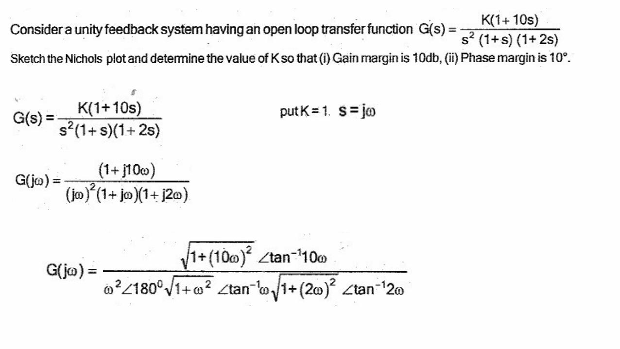
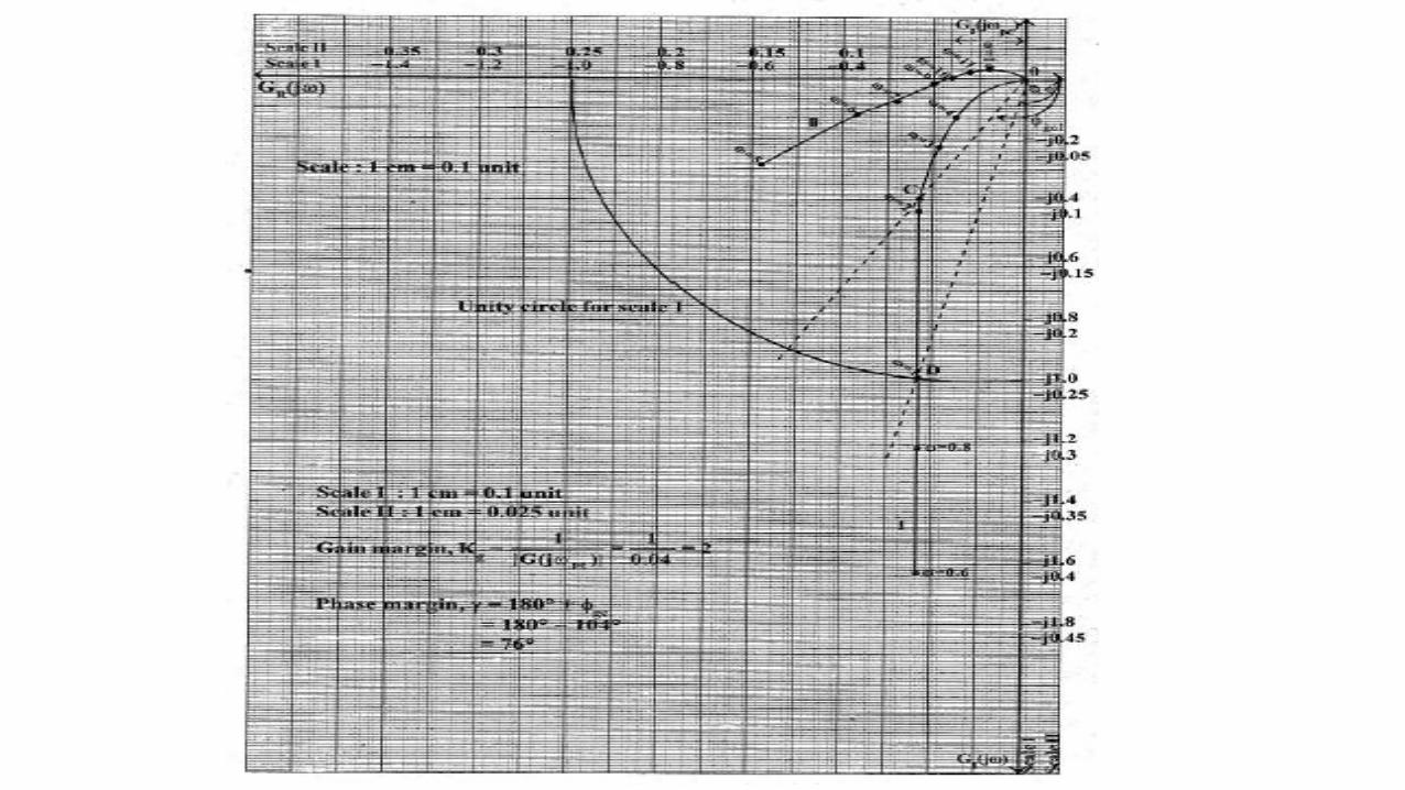
NICHOLS PLOT

The Nichols plot is a frequency response plot of the open loop transfer function of a system.

The Nichols plot is a graph between magnitude of in db and the phase of in

degree, plotted on a ordinary graph sheet.

Steps

Consider open loop transfer function of the given system

Obtain the expression for in terms of

Obtain the expression for in terms of

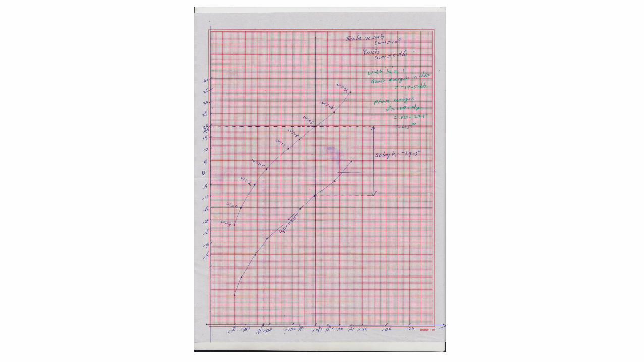
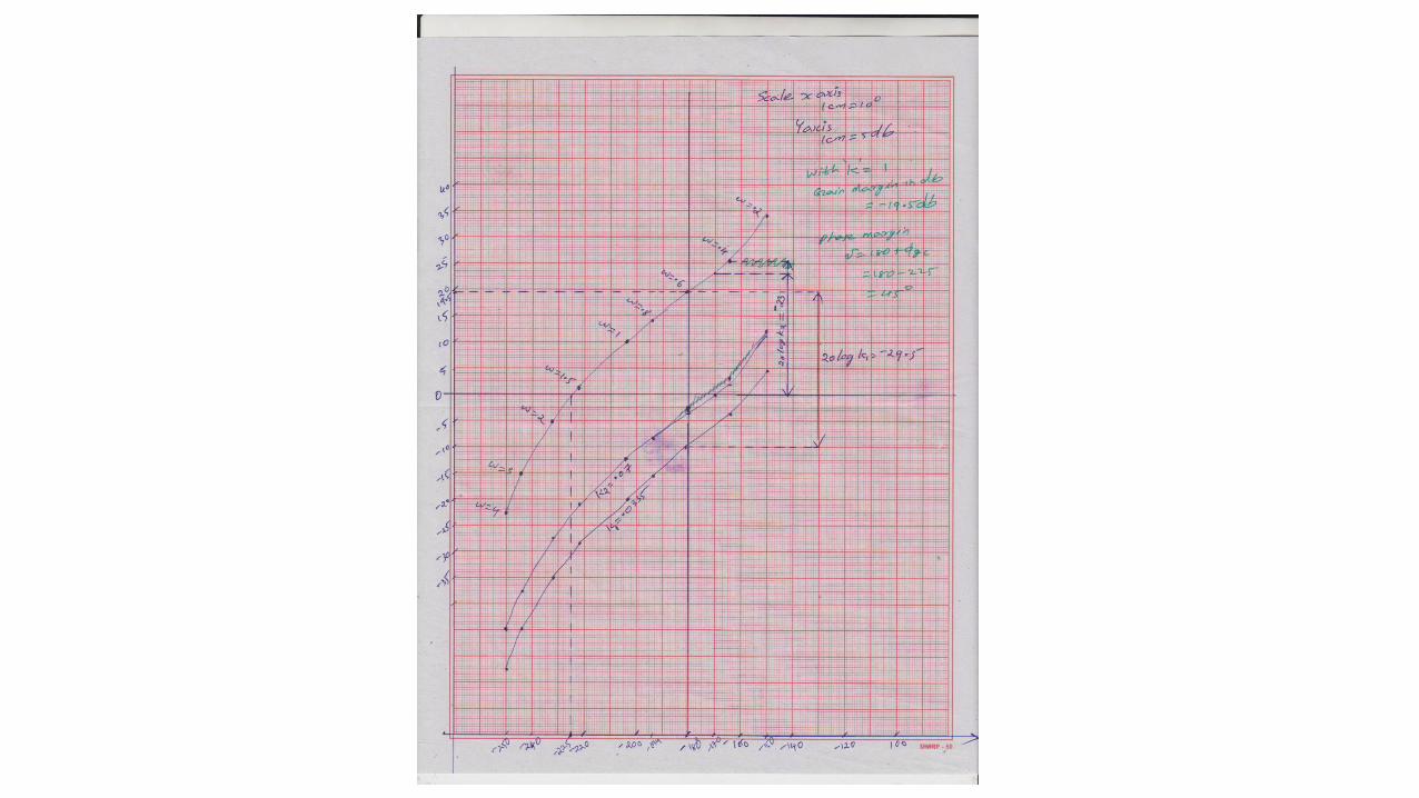
Tabulate the values of magnitude expressed in db and angle in degree for various values of

Select suitable scale on an ordinary graph paper with Y-axis representing magnitude in db and

X-axis representing phase angle in degrees

Plot all the points tabulated on the graph paper.

The smooth curve obtained by joining all such plotted points represents magnitude-phase plot

of a given system.

The gain margin in db is given by the negative of magnitude of at the phase cross over

frequency . The is the frequency at at which phase of is -180 degree.

If the db magnitude of at is negative then gain margin is positive and vice

versa

Let be the phase angle of at gain cross over frequency .

The is the frequency at which the db magnitude of is zero.

Now the phase margin is given by .

If is less negative than -180 degree then phase margin is positive and vice versa.

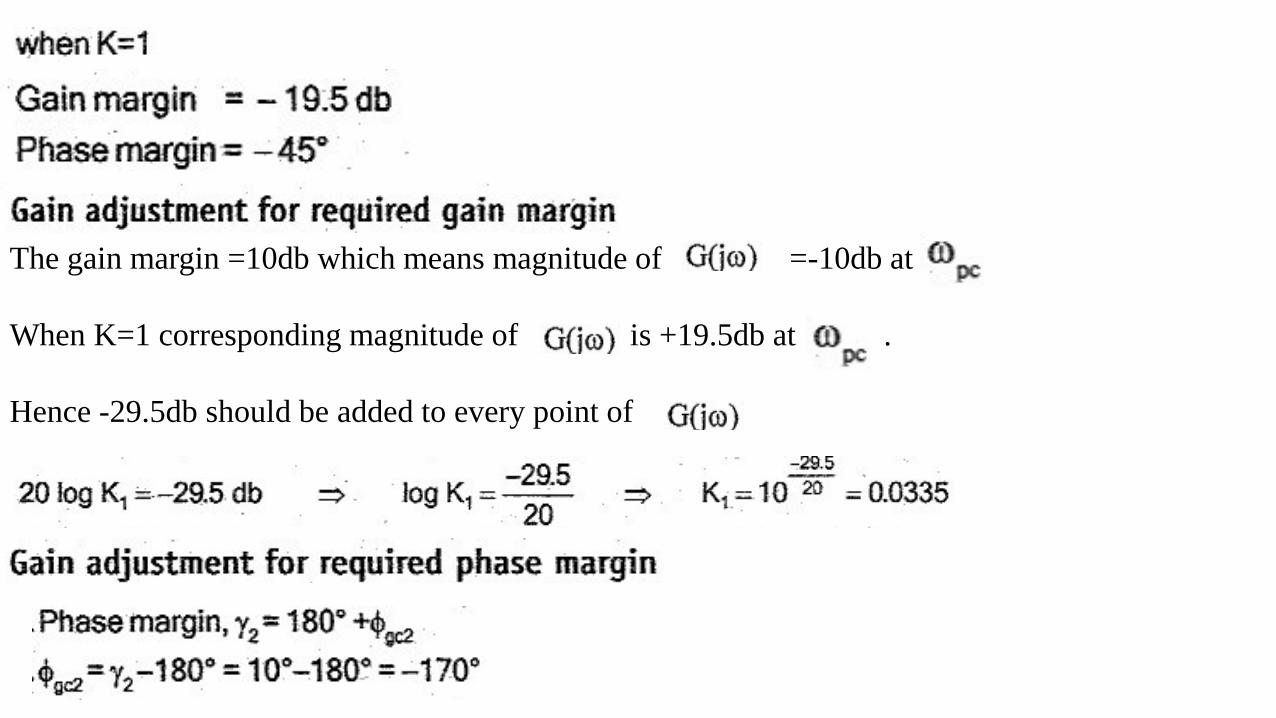
The gain margin =10db which means magnitude of =-10db at

When K=1 corresponding magnitude of is +19.5db at .

Hence -29.5db should be added to every point of

When K=1 corresponding magnitude of is +23db at -170 degree.

But for a phase margin of 10 degree, this gain should be made zero.

Hence -23db should be added to every point of

MODULE VI

Polar plot

Nyquist stability criterion

Nichols chart

Non-minimum phase system

transportation lag

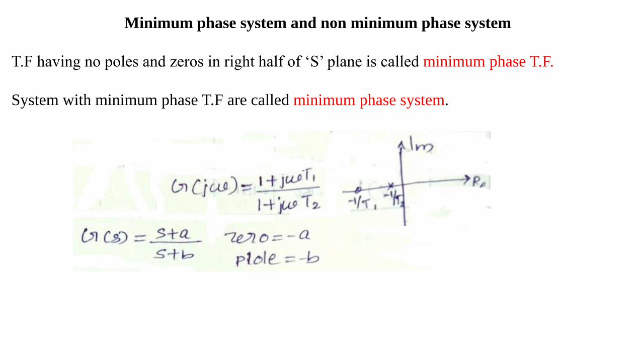
Minimum phase system and non minimum phase system

T.F having no poles and zeros in right half of ‘S’ plane is called minimum phase T.F.

System with minimum phase T.F are called minimum phase system.

The T.F having poles and/or zeros in the right half of ‘S’ plane are called non minimum phase

T.F.

System with non minimum phase T.F are called non minimum phase system

Transportation Lag

It is also called dead time or time delay.

In practical systems due to several reasons, it is necessary to stop certain action in a system for some time.

Such time delay is called transportation lag.

For example in modern systems using micro controllers, it is difficult to match the speed of peripherals with micro controller.

In such a case it is necessary to provide purposely a time delay to micro controllers to adjust with the speed of other supporting peripherals.

The transportation lag is given by the expression in Laplace domain

Tj-

Ts

Ts

e)e(j

eG(S)

e

Tse

dB 0log1 20dBin

1ωTsinωTcos)

ωTsin jcosθe

sinθ jcosθe

)

22

jω

jθ

ωT

G(jω

ee(jω -j

Introducing time delay in system has no effect on the magnitude plot.

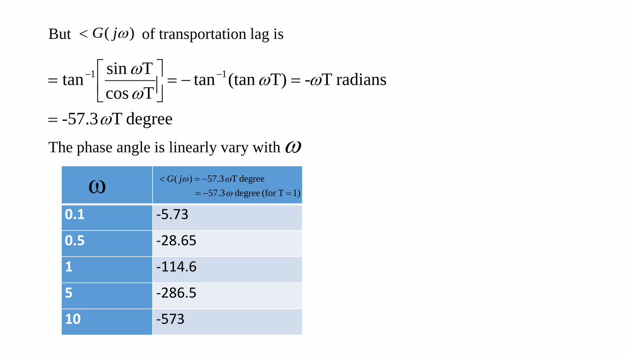
But of transportation lag is

The phase angle is linearly vary with

degree T -57.3

radians T-T) (tantanT cos

T sintan 11

)( jG

0.1 -5.73

0.5 -28.65

1 -114.6

5 -286.5

10 -573

ω 1)T(for degree 3.57

degree T 3.57)(

jG

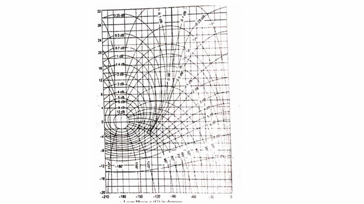
Nichols chart

Nichols transformed the constant M and N circle contours on the polar plots to log magnitude

versus phase angle plot.

M circles are called constant magnitude loci while N circles are called as constant phase

angle loci

The frequency response characteristics of a system can be studied by plotting the log

magnitude in dB versus the phase angle for various frequencies.

When the open loop gain in dB versus loop phase angle in degree is plotted for different

frequencies and M and N circles are superimposed on it, the resultant plot thus obtained is

called Nichols chart

With the help of Nichols chart the following can be evaluated:

1. Complete closed loop frequency response.

2. Parameters M, bandwidth, gain and can be calculated for the closed loop systemω

The Nichols chart may be thought of as a Nyquist plot on a log scale.

A Nyquist plot is a plot in the complex plane of

Instead, on a Nichols chart, we plot

Notice that we reverse the coordinates -the real part is plotted on the vertical, and the

imaginary part is plotted on the horizontal.

In addition, the chart has contours of constant closed-loop magnitude and phase,