Revision: 3-12 1 Module 9: Nonparametric Statistics Statistics (OA3102) Professor Ron Fricker Naval Postgraduate School Monterey, California Reading assignment: WM&S chapter 15.1-15.6

Welcome message from author
This document is posted to help you gain knowledge. Please leave a comment to let me know what you think about it! Share it to your friends and learn new things together.
Transcript

Revision: 3-12 1
Module 9:
Nonparametric Statistics Statistics (OA3102)
Professor Ron Fricker Naval Postgraduate School
Monterey, California
Reading assignment:
WM&S chapter 15.1-15.6

2
Goals for this Lecture
• Discuss advantages and disadvantages of nonparametric tests – General two-sample shift model
• Nonparametric tests for paired data – Sign test
– Wilcoxon signed-rank test
• Small and large sample variants
• Nonparametric tests for two-samples of independent data – Wilcoxon rank sum test
– Mann-Whitney U test
Revision: 3-12
Challenges in Hypothesis Testing
• Some experiments give responses they defy
exact quantification
– Rank the “utility” of four weapons systems
• Gives an ordering, but can be impossible to say
things like “System A is twice as useful as B”
– Compare two LVS maintenance programs
• If the data clearly do not fit the assumptions of
the (parametric) tests we have learned, what to
do?
• Nonparametric tests may be the solution
Revision: 3-12 3

4
Parametric vs. Nonparametric
• Parametric hypothesis testing: – Statistic distribution are specified (often normal)
– Often follows from Central Limit Theorem, but sometimes CLT assumptions don’t fit/apply
• Nonparametric hypothesis testing: – Does not assume a particular probability
distribution
• Often called “distribution free”
– Generally based on ordering or order statistics
Revision: 3-12

5
Advantages of Nonparametric Tests
• Tests make less stringent demands on the
data
– E.g., they require fewer assumptions
• Usually require independent observations
• Sometimes assume continuity of the measure
• Can be more appropriate:
– When measures are not precise
– For ordinal data where scale is not obvious
– When only ordering of data is available
Revision: 3-12

6
Disadvantages of Nonparametric Tests
• They may “throw away” information – E.g., Sign tests only looks at the signs (+ or -) of
the data, not the numeric values
– If the other information is available and there is an appropriate parametric test, that test will be more powerful
• The trade-off: – Parametric tests are more powerful if the
assumptions are met
– Nonparametric tests provide a more general result if they are powerful enough to reject
Revision: 3-12

A General Two-Sample Shift Model
• Consider two independent samples of data,
, taken from normal
populations with means mX and mY and equal
variances
• Then we may wish to test
• This is a two-sample parametric shift (or
location) model
– Parametric as the distribution is specified (normal)
– All is known except mX and mY (and perhaps s2)
Revision: 3-12 7
1 21 1,..., and ,...,n nX X Y Y
0 : 0 vs. : 0X Y a X YH Hm m m m

Now, Generalizing to a
Nonparametric Shift Model
• Let be a random sample from a
population with distribution function F(x)
• Let be a random sample from a
population with distribution function G(y)
• Consider testing the hypotheses that the two
distributions are the same,
where the form of the distributions is
unspecified
– A nonparametric approach now clearly required
Revision: 3-12 8
11,..., nX X
0 : ( ) ( ) vs. : ( ) ( )aH F z G z H F z G z
21,..., nY Y

Generalizing to a Nonparametric
Shift Model (continued)
• Notice that the hypotheses
are very broad
– It just says the two distributions are different
• Often experimenters want to test something
more specific, such as the distributions differ
by location
– E.g.,
– See Figure 15.2 in the text for an illustration
Revision: 3-12 9
0 : ( ) ( ) vs. : ( ) ( )aH F z G z H F z G z
( ) =Pr( )=Pr( ) ( )G y Y y X y F y
Generalizing to a Nonparametric
Shift Model (continued)
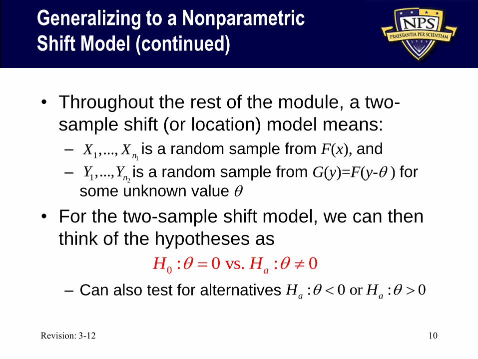
• Throughout the rest of the module, a two-
sample shift (or location) model means:
– is a random sample from F(x), and
– is a random sample from G(y)=F(y- ) for
some unknown value
• For the two-sample shift model, we can then
think of the hypotheses as
– Can also test for alternatives
Revision: 3-12 10
11,..., nX X
21,..., nY Y
0 : 0 vs. : 0aH H
: 0 or : 0a aH H

Introduction to the Sign Test
for a Matched Pairs Experiment
• Suppose there are n pairs of observations in
the form (Xi, Yi)
• We wish to test the hypothesis that the
distribution of the Xs and Ys is the same
except perhaps for the location
• One of the simplest nonparametric tests is
called the sign test
– Idea: Define Di = Xi –Yi. Then under the null
hypothesis, the probability that Di is positive is 0.5
Revision: 3-12 11
Revision: 3-12 12
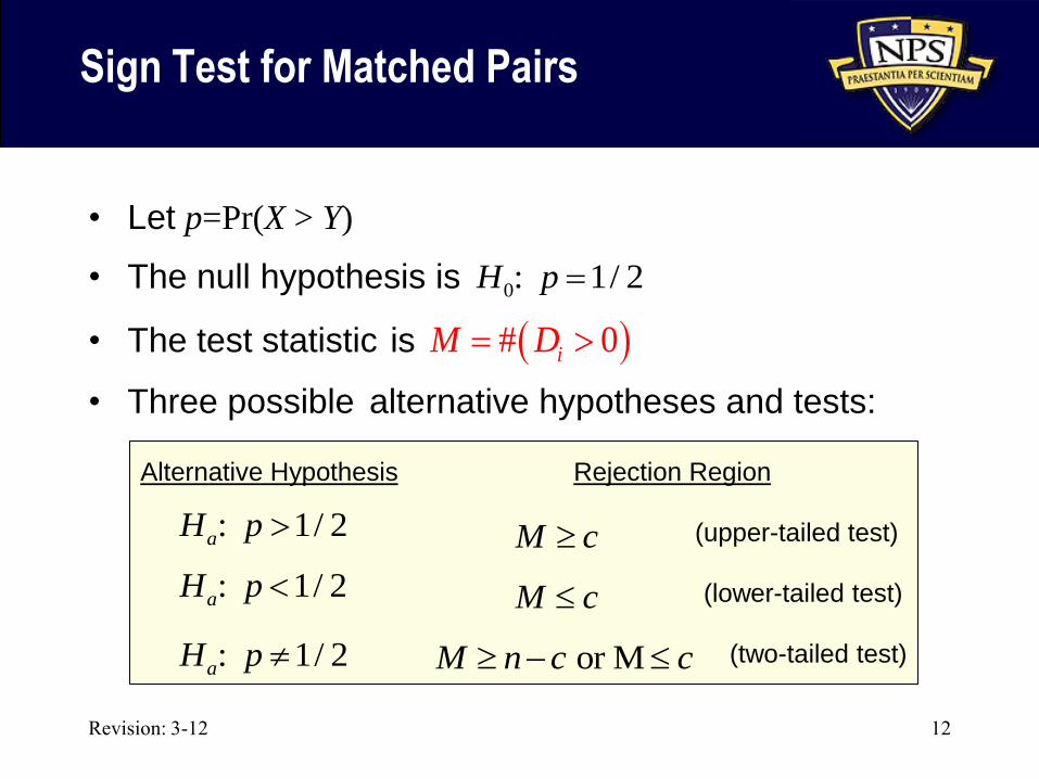
Sign Test for Matched Pairs
• Let p=Pr(X > Y)
• The null hypothesis is
• The test statistic is
• Three possible alternative hypotheses and tests:
# 0iM D
: 1/ 2aH p
: 1/ 2aH p
: 1/ 2aH p
Alternative Hypothesis Rejection Region
M c
M c
or MM n c c
(upper-tailed test)
(lower-tailed test)
(two-tailed test)
0: 1/ 2H p
Revision: 3-12 13
Example 15.1
• Number of defective electrical fuses for each
of two production lines recorded daily for 10
days
• Is there sufficient evidence to say that one
line produces more defectives than the other?
• Write out the hypotheses:

Example 15.1 (continued)
• Now, calculate the test statistic:
Revision: 3-12 14
Day A B
1 172 201
2 165 179
3 206 159
4 184 192
5 174 177
6 142 170
7 190 182
8 169 179
9 161 169
10 200 201

Example 15.1 (continued)
• And now determine the rejection region for a
test of level 0.05 < a < 0.1
Revision: 3-12 15

Example 15.1 (continued)
• And, finally, conduct the test
– What do you conclude?
Revision: 3-12 16

Example 15.2
• Find the p-value for the test in Example 15.1
Revision: 3-12 17
In R
Revision: 3-12 18
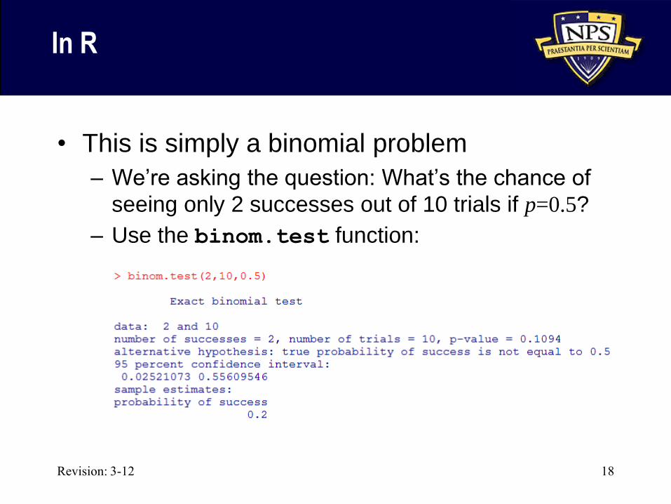
• This is simply a binomial problem
– We’re asking the question: What’s the chance of
seeing only 2 successes out of 10 trials if p=0.5?
– Use the binom.test function:

An Aside:
A Parametric Test, the Paired t-Test
Revision: 3-12 19
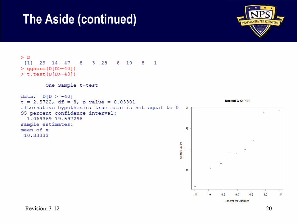
The Aside (continued)
Revision: 3-12 20
Issues and Variants
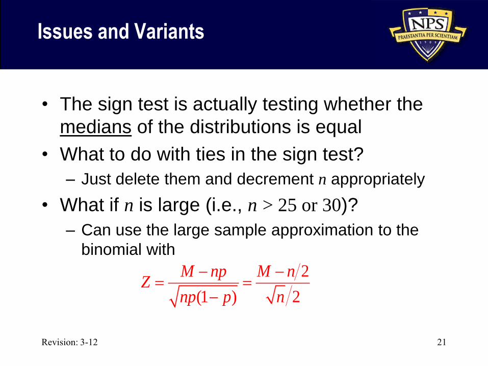
• The sign test is actually testing whether the
medians of the distributions is equal
• What to do with ties in the sign test?
– Just delete them and decrement n appropriately
• What if n is large (i.e., n > 25 or 30)?
– Can use the large sample approximation to the
binomial with
Revision: 3-12 21
2
(1 ) 2
M np M nZ
np p n

Revision: 3-12 22
Sign Test for Large Samples (n > 25)
• Let p=Pr(X > Y)
• The null hypothesis is
• The test statistic is
• Three possible alternative hypotheses and tests:
: 1/ 2aH p
: 1/ 2aH p
: 1/ 2aH p
Alternative Hypothesis
(upper-tailed test)
(lower-tailed test)
(two-tailed test)
0: 1/ 2H p
2 0.5Z M n n
Rejection Region for Level a Test
z za
z za
/ 2 / 2 or z z z za a

23
Wilcoxon Signed-Rank Test
• One- or two-sided test for the hypotheses of
the means of a paired sample: (Xi, Yi )
– Unlike the sign test, here we also use the
information contained in the magnitude of the
differences, Di =Yi – Xi , i = 1,…,n
– I.e., we’ll use the ranks of the absolute values of
the differences in the test, not just the signs
• Hypotheses:
– H0: the distributions of the Xs and Ys are identical
– Ha: the population distributions differ in location
(two-tailed) or population distribution for Xs is
shifted to the right (one-tailed)

24
Signed-Rank Methodology
• To conduct the test:
– For n matched pairs, one observation from each
population (Xi, Yi ), define Di =Yi – Xi
– Compute the signed ranks: Ri=sign(Di) R(|Di|)
• R(|Di|) is the rank of |Di| among the n Dis
• Give tied observations the average rank
• If doing the calculation by hand, build a table:
i X Y Di =Xi – Yi |Di| R(|Di|) Ri=sign(Di) R(|Di|)
1
2

25
The Test Statistic
• For a one-sided test:
To test if the Xs are shifted to the right of the Ys,
use T=T-, the sum of the negative signed ranks
To test if the Ys are shifted to the right of the Xs,
use T=T+, the sum of the positive signed ranks
• For a two-sided test, the test statistic is
T=min(T+,T-), the minimum of either the sum
of the positive or negative signed ranks

The Rejection Region
• Use Table 9:
Revision: 3-12 26

Revision: 3-12 27
Example 15.3
• Because of the variations in ovens, two types
of cake mix were tested in six different ovens
– So, each oven was used to bake each type of mix
(“A” and “B”)
– It’s a paired experimental design (by oven)
• Using the Wilcoxon signed-rank test, test the
hypothesis that there is no difference in the
population distribution of cake densities
between the two mixes
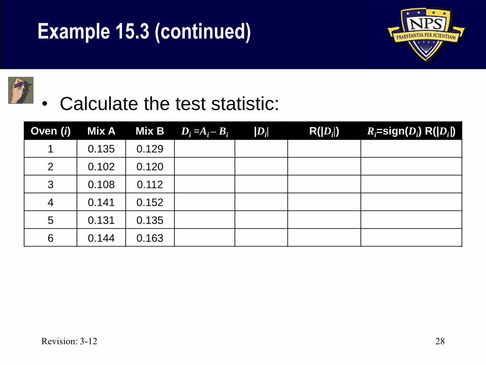
Example 15.3 (continued)
• Calculate the test statistic:
Revision: 3-12 28
Oven (i) Mix A Mix B Di =Ai – Bi |Di| R(|Di|) Ri=sign(Di) R(|Di|)
1 0.135 0.129
2 0.102 0.120
3 0.108 0.112
4 0.141 0.152
5 0.131 0.135
6 0.144 0.163

Example 15.3 (continued)
• Determine the test outcome
Revision: 3-12 29

30
Large Sample
Wilcoxon Signed-Rank Test
• When n > 25, can use normal approximation
• It turns out that
• So we can use the test statistic
( 1) / 4
( 1)(2 1) / 24Var( )
T E T T n nZ
n n nT
1 / 4E T n n
Var 1 2 1 / 24T n n n
Revision: 3-12 31
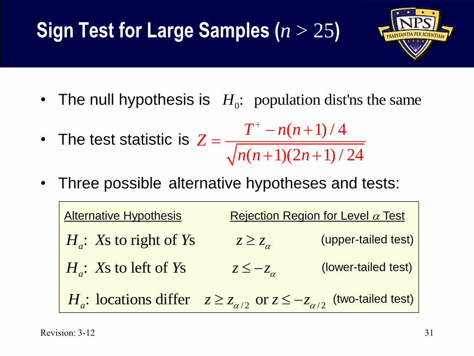
Sign Test for Large Samples (n > 25)
• The null hypothesis is
• The test statistic is
• Three possible alternative hypotheses and tests:
: s to right of saH X Y
: s to left of saH X Y
: locations differaH
Alternative Hypothesis
(upper-tailed test)
(lower-tailed test)
(two-tailed test)
0: population dist'ns the sameH
Rejection Region for Level a Test
z za
z za
/ 2 / 2 or z z z za a
( 1) / 4
( 1)(2 1) / 24
T n nZ
n n n

Wilcoxon Rank Sum Test
• Now, consider two independent samples of
data, , where goal is to
test whether population dist’ns are the same
• Idea: Pool the n1+n2=n observations, rank
them in order of magnitude, and then sum
their ranks of the Xs and Ys
– Under the null hypothesis (distributions are the
same) the sum of the ranks should be about equal
– If there is a location shift, one of the sums should
be larger
Revision: 3-12 32
1 21 1,..., and ,...,n nX X Y Y

Wilcoxon Rank Sum Test (cont’d)
• The hypotheses are like before:
– H0: the distributions of the Xs and Ys are identical
– Ha: the population distributions differ in location
• Either two-tailed or one tailed
• An equivalent test: Mann-Whitney U test
– We’ll get to that next…
Revision: 3-12 33
Revision: 3-12 34
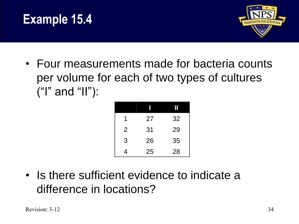
Example 15.4
• Four measurements made for bacteria counts
per volume for each of two types of cultures
(“I” and “II”):
• Is there sufficient evidence to indicate a
difference in locations?
I II
1 27 32
2 31 29
3 26 35
4 25 28
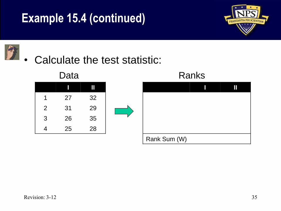
Example 15.4 (continued)
• Calculate the test statistic:
Revision: 3-12 35
I II
1 27 32
2 31 29
3 26 35
4 25 28
I II
Rank Sum (W)
Data Ranks

Example 15.4 (continued)
• And now determine the rejection region
Revision: 3-12 36

Example 15.4 (continued)
Revision: 3-12 37

Example 15.4 (continued)
• And, finally, conduct the test
– What do you conclude?
Revision: 3-12 38

The Mann-Whitney U Test
• As with the Wilcoxon rank sum test, this test
is based on two independent samples of
data,
• Again, the goal is to test whether population
dist’ns are the same
• Idea: Order the n1+n2 observations and count
the number of X observations that are smaller
then each of the Y observations
Revision: 3-12 39
1 21 1,..., and ,...,n nX X Y Y

Example
• From Example 15.4, the eight ordered
observations are:
• So:
– u1=3 since there are three Xs before y(1)
– u2=3 since there are three Xs before y(2)
– u3=4 since there are three Xs before y(3)
– u4=4 since there are three Xs before y(4)
• And thus U = u1+u2+u3+u4 = 3+3+4+4 = 14
Revision: 3-12 40
25 26 27 28 29 31 32 35
x(1) x(2) x(3) y(1) y(2) x(4) y(3) y(4)
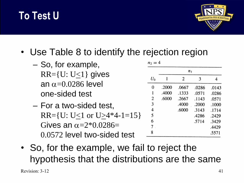
To Test U
• Use Table 8 to identify the rejection region
– So, for example,
RR={U: U<1} gives
an a=0.0286 level
one-sided test
– For a two-sided test,
RR={U: U<1 or U>4*4-1=15}
Gives an a=2*0.0286=
0.0572 level two-sided test
• So, for the example, we fail to reject the
hypothesis that the distributions are the same Revision: 3-12 41

Mann-Whitney U vs. Rank Sum Test
• Turns out the two tests are directly related:
where
n1 is the number of X observations
n2 is the number of Y observations
W is the rank sum for the Xs
• So, first calculate the rank sums of the Xs and
then calculate U
Revision: 3-12 42
1 1
1 2
1
2
n nU n n W
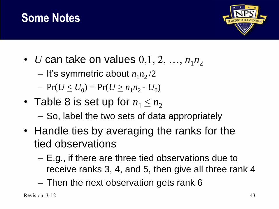
Some Notes
• U can take on values 0,1, 2, …, n1n2
– It’s symmetric about n1n2 /2
– Pr(U < U0) = Pr(U > n1n2 - U0)
• Table 8 is set up for n1 < n2
– So, label the two sets of data appropriately
• Handle ties by averaging the ranks for the
tied observations
– E.g., if there are three tied observations due to
receive ranks 3, 4, and 5, then give all three rank 4
– Then the next observation gets rank 6
Revision: 3-12 43

Revision: 3-12 44
Mann-Whitney U Test
• The null hypothesis is
• The test statistic is
• Three possible alternative hypotheses and tests:
: s to right of saH X Y
: s to left of saH X Y
: locations differaH
Alternative Hypothesis
(upper-tailed test)
(lower-tailed test)
(two-tailed test)
0: population dist'ns the sameH
Rejection Region
0U U
1 2 0U n n U
0 1 2 0 or U U U n n U
1 1
1 2
1
2
n nU n n W
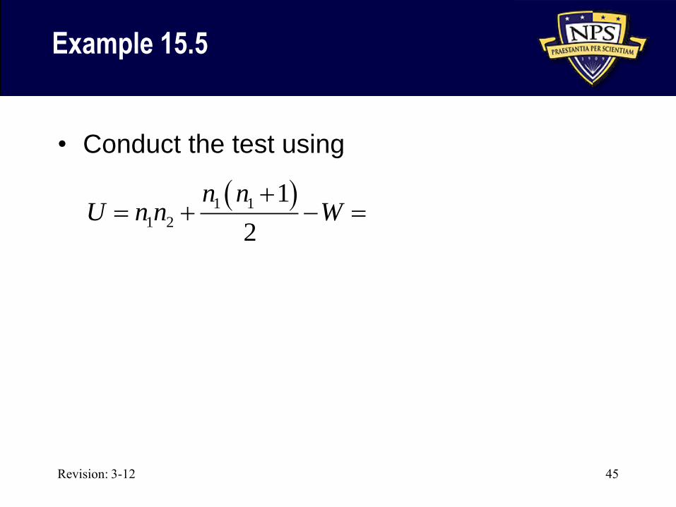
Example 15.5
• Conduct the test using
Revision: 3-12 45
1 1
1 2
1
2
n nU n n W

Example 15.6
• An experiment was conducted to compare
the strengths of two types of kraft paper (i.e.,
cardboard)
– Standard kraft paper
– Paper treated with a chemical substance
• Test the hypothesis of no difference in the
distributions of the strength of the papers
versus the alternative that the treated paper
tends to be stronger
Revision: 3-12 46

Example 15.6 (continued)
• Calculate the test statistic:
Revision: 3-12 47
Standard,
I
Treated,
II
1 1.21 (2) 1.49 (15)
2 1.43 (12) 1.37 (7.5)
3 1.35 (6) 1.67 (20)
4 1.51 (17) 1.50 (16)
5 1.39 (9) 1.31 (5)
6 1.17 (1) 1.29 (3.5)
7 1.48 (14) 1.52 (18)
8 1.42 (11) 1.37 (7.5)
9 21.29 (3.5) 1.44 (13)
10 1.40 (10) 1.53 (19)
Rank
Sum
W=85.5
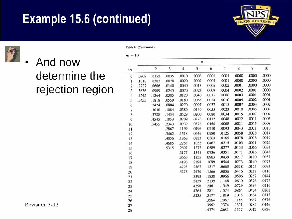
Example 15.6 (continued)
• And now
determine the
rejection region
Revision: 3-12 48
Example 15.6 (continued)
• And, finally, conduct the test
– What do you conclude?
Revision: 3-12 49

50
Large Sample
Mann-Whitney U Test
• When n1 > 10 and n2 > 10, can use normal
approximation
• It turns out that
• So we can use the test statistic
1 2
1 2 1 2
/ 2
Var( ) 1 /12
U E U U n nZ
U n n n n
1 2 / 2E U n n
1 2 1 2Var 1 /12U n n n n

Revision: 3-12 51
Large Sample U Test (n1 > 10, n2 > 10)
• The null hypothesis is
• The test statistic is
• Three possible alternative hypotheses and tests:
: s to left of saH X Y
: s to right of saH X Y
: locations differaH
Alternative Hypothesis
(upper-tailed test)
(lower-tailed test)
(two-tailed test)
0: population dist'ns the sameH
Rejection Region for Level a Test
z za
z za
/ 2 / 2 or z z z za a
1 2
1 2 1 2
/ 2
1 /12
U n nZ
n n n n
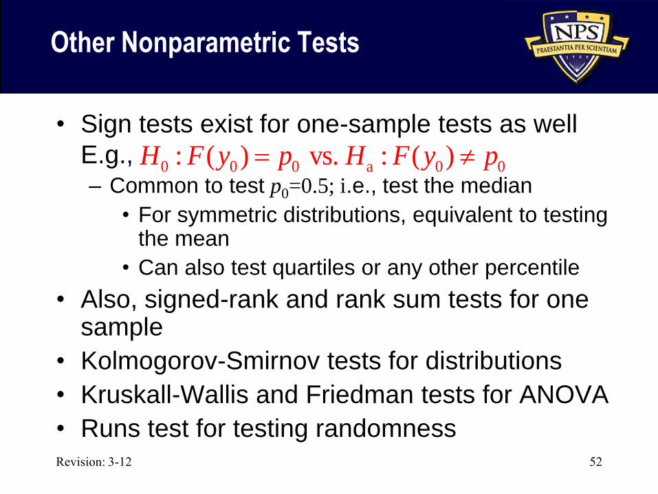
Other Nonparametric Tests
• Sign tests exist for one-sample tests as well
E.g., – Common to test p0=0.5; i.e., test the median
• For symmetric distributions, equivalent to testing the mean
• Can also test quartiles or any other percentile
• Also, signed-rank and rank sum tests for one sample
• Kolmogorov-Smirnov tests for distributions
• Kruskall-Wallis and Friedman tests for ANOVA
• Runs test for testing randomness
Revision: 3-12 52
0 0 0 a 0 0: ( ) vs. : ( )H F y p H F y p

What We Covered in this Module
• Discussed advantages and disadvantages of nonparametric tests – Described the general two-sample shift model
• Nonparametric tests for paired data – Sign test
– Wilcoxon signed-rank test
• Small and large sample variants
• Nonparametric tests for two-samples of independent data – Wilcoxon rank sum test
– Mann-Whitney U test
Revision: 3-12 53
Revision: 3-12 54
Homework
• WM&S chapter 15
– Required: 4, 9, 13, 17, 23, 25, 27
– Extra credit: None
Related Documents