module 1 (Mechanics)

E-CONTENT

ON

MECHANICS OF SOLIDS-I

BTME 1205

(L 3 - T 1 - P 0)

FOR

2ND SEMESTER

2012-13

DEPARTMENT OF MECHANICAL ENGINEERING

Centurion University of Technology & Management

PARALAKHEMUNDI GAJAPATI

ODISHA – 761211

MODULE-1

Table of contents

Lecture – 1 INTRODUCTION TO ENGINEERING MECHANICS 1

Lecture – 2 SYSTEM OF FORCESFORCE 4

Lecture – 3 PARALLELOGRAM LAW OF FORCES 9

Lecture – 4 COMPOSITION OF FORCES 11

Lecture – 5 MOMENT 14

Lecture – 6 EQUILIBRIUM 16

Lecture – 7 LAMI’S THEOREM 19

Lecture – 8 CENTROID 19

Lecture – 9 CENTRIIID OF AN ARC OF A CIRCLE 21

Lecture – 10 CENTRE OF GRAVITY AND CENTROID 22

Lecture – 11 CENTROID OF A SEMICIRCLE 24

Lecture – 12 CENTROID OF COMPOSITE SECTIONS 28

Lecture – 13 THEOREMS OF PAPPUS 29

Lecture – 14 MOMENT OF INERTIA 32

Lecture – 15 MOMENT OF INERTIA OF STANDARD SECTIONS 34

Lecture – 16 MOMENT OF INERTIA OF COMPOSITE SECTIONS 38

Lecture – 17 PRODUCTS OF INERTIA 40

Lecture – 18 FRICTION 41

Lecture – 19 BODY ON A ROUGH HORIZONTAL 43

Lecture – 20 SCREW JACK 45

Lecture – 21 BELT FRICTION 47

Lecture – 22 Single-purchase crab winch 50

Lecture – 23 Wedge and Block Friction 51

Lecture – 24 SIMPLE MACHINES 52

1

Lecture – 1

INTRODUCTION TO ENGINEERING MECHANICS

Mechanics can be defined as that science which describes and predicts the conditions of rest or

motion of bodies under the action of forces. With roots in physics and mathematics, Engineering

Mechanics is the basis of all the mechanical sciences: civil engineering, materials science and

engineering, mechanical engineering and aeronautical and aerospace engineering. Engineering

Mechanics provides the "building blocks" of statics, dynamics, strength of materials, and fluid

dynamics.

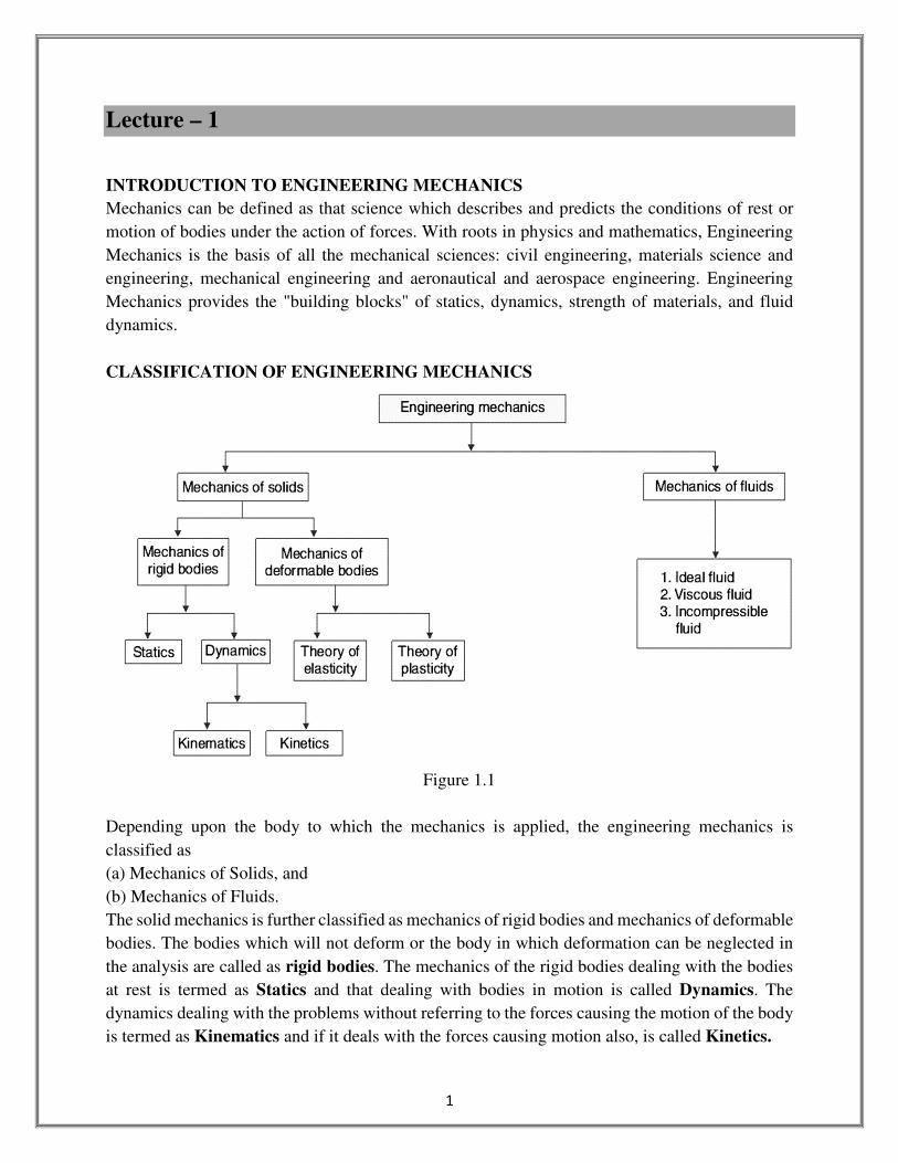
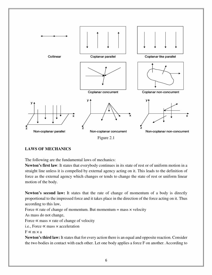
CLASSIFICATION OF ENGINEERING MECHANICS

Figure 1.1

Depending upon the body to which the mechanics is applied, the engineering mechanics is

classified as

(a) Mechanics of Solids, and

(b) Mechanics of Fluids.

The solid mechanics is further classified as mechanics of rigid bodies and mechanics of deformable

bodies. The bodies which will not deform or the body in which deformation can be neglected in

the analysis are called as rigid bodies. The mechanics of the rigid bodies dealing with the bodies

at rest is termed as Statics and that dealing with bodies in motion is called Dynamics. The

dynamics dealing with the problems without referring to the forces causing the motion of the body

is termed as Kinematics and if it deals with the forces causing motion also, is called Kinetics.

2

If the internal stresses developed in a body are to be studied, the deformation of the body should

be considered. This field of mechanics is called Mechanics of Deformable Bodies/ Strength of

Materials/Solid Mechanics. This field may be further divided into Theory of Elasticity and Theory

of Plasticity.

Liquid and gases deform continuously with application of very small shear forces. Such materials

are called Fluids. The mechanics dealing with behavior of such materials is called Fluid

Mechanics. Mechanics of ideal fluids, mechanics of viscous fluid and mechanics of incompressible

fluids are further classification in this area. The classification of mechanics is summarized above

in flow chart.

In mechanics we look at real life situations and try to predict what will happen. The problem with

real life is that it is often quite complicated. When studying problems in mechanics we often make

idealizations of real life situations that simplify the problem. There are many commonly used

idealizations that we will introduce in later sheets. Here follows a list of some common

idealizations that are used in mechanics.

IDEALISATIONS IN MECHANICS

A number of ideal conditions are assumed to exist while applying the laws of mechanics of

practical problems. In fact, without such assumptions, it is not feasible to arrive at practical

solutions. The experience in the past centuries has shown that the following idealization could be

made as they do not bring down the accuracy of the analytical results below the optimum level

required by engineers to deal with practical diagram.

CONTINUUM: A body consists of several particles. It is a well-known fact that each particle can

be sub-divided into molecules, atoms and electrons. It is not feasible to solve any engineering

problem by treating a body as a conglomeration of such discrete particles. The body is assumed

to consist of a continuous distribution of matter which will not separate even when various

forces considered are acting simultaneously. In other words, we say the body is treated as a

continuum.

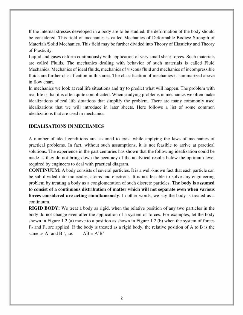
RIGID BODY: We treat a body as rigid, when the relative position of any two particles in the

body do not change even after the application of a system of forces. For examples, let the body

shown in Figure 1.2 (a) move to a position as shown in Figure 1.2 (b) when the system of forces

F2 and F3 are applied. If the body is treated as a rigid body, the relative position of A to B is the

same as A’ and B ’, i.e. AB = A’B’

3

Figure 1.2

PARTICLE: A particle may be defined as an object which has only mass and no size.

Theoretically, such a body cannot exist; while dealing with the problems involving distances which

are considerably larger compared to the size of the body, the size of the body may be neglected

without sacrificing the accuracy, the example are as follows:

• A bomber aero-plane is a particle for a gunner operating from the ground.

• A ship in a mid-sea is a particle in the study of relative motion from the control in a part.

• In the study of the movement of earth in celestial space, earth is treated as a particle.

SYSTEM OF PARTICLES: A system of particles means a group of particles inter-related. The

equations for a system of particles can be readily used to develop those for a rigid body.

BASIC CONCEPTS USED IN MECHANICS

We have learnt in Introduction to Engineering Mechanics that mechanics is the study of physical

objects, their state of rest and motion and interactions of physical bodies. Study of these attributes

of physical bodies requires some basic concepts to define the physical world. These are space,

time, mass and force. These basic concepts are the building blocks of Engineering Mechanics and

the framework upon which the study of mechanics will be based upon.

Space: To define position of physical bodies and their extent we rely on the basic concept of space.

The objects under consideration in mechanics have some position in space and occupy some part

of the space. Position of any object is defined relative to a reference point, called the origin. The

position of any object is specified by linear and angular distances of the object from the origin in

different directions.

Time: In mechanics we also study events. To define which event occurred when, sequence of

events and duration of events we have conceived the notion of time. The concept of time is not

used directly in statics but in dynamics it plays an important role.

4

Mass: Every physical body has some inertia, which is, they offer resistance to the change in their

course of motion. And physical bodies attract each other with a certain force called as gravitational

force. These attributes of physical bodies are assigned to the concept of mass. As per the concept

of mass each body has certain amount of mass which causes the inertia and gravitational attraction.

Force: Interaction between physical bodies is seen in terms of force acting between them. This

interaction can be through contact, like books placed on a table, or without contact, like

gravitational pull. Force is defined by its magnitude, direction and point of application. Force

acting on a body tends to move it in the direction of force.

These four basic concepts of space, time, mass and force form the base for the study of mechanics.

To use these concepts for analysis of rest and motion of the physical bodies we need to quantify

them. In a latter article we will learn how these concepts are quantified and how units are defined

for them.

Lecture – 2

SYSTEM OF FORCESFORCE

From Newton’s first law, we defined the force as the agency which tries to change state of stress

or state of uniform motion of the body. From Newton’s second law of motion we arrived at

practical definition of unit force as the force required producing unit acceleration in a body of unit

mass. Thus 1 Newton is the force required to produce an acceleration of 1 m/sec2 in a body of 1

kg mass. It may be noted that a force is completely specified only when the following four

characteristics are specified:

(a) Magnitude (b) Point of application (c) Line of action, and Direction

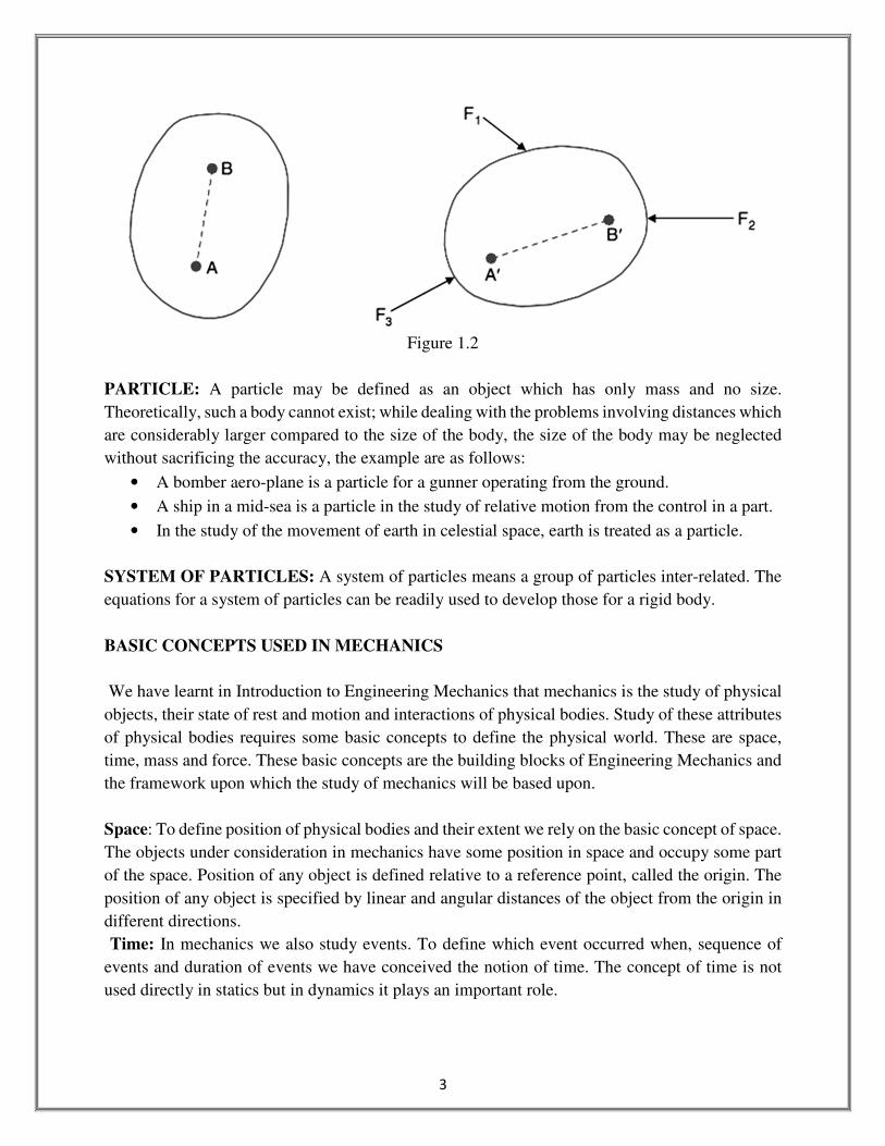
When several forces act simultaneously on a body, they constitute a system of forces. If all the

forces in a system do not lie in a single plane they constitute the system of forces in space. If all

the forces in a system lie in a single plane, it is called a coplanar force system. If the line of action

of all the forces in a system passes through a single point, it is called a concurrent force system. In

a system of parallel forces all the forces are parallel to each other. If the lines of action of all the

forces lie along a single line then it is called a collinear force system. Various system of forces,

their characteristics and examples are given in Table 2.1 and shown in Figure 2.1.

5

Table 2.1: System of Forces

Force System Characteristics Examples

Collinear forces Line of action of all the forces

act along the same line.

Forces on a rope in a tug of

war.

Coplanar parallel forces

All forces are parallel to each

other and lie in a single plane.

System of forces acting on a

beam subjected to vertical

loads (including reactions).

Coplanar like parallel forces

All forces are parallel to each

other, lie in a single plane and

are acting in the same

direction.

Weight of a stationary train

on a rail when the track is

straight.

Coplanar concurrent forces

Line of action of all forces

pass through a single point

and forces lie in the same

plane.

Forces on a rod resting

against a wall.

Coplanar non-concurrent

forces

All forces do not meet at a

point, but lie in a single plane.

Forces on a ladder resting

against a wall when a person

stands on a rung which is not

at its centre of gravity.

Non-coplanar parallel forces

All the forces are parallel to

each other, hut not in same

plane.

The weight of benches in a

class room.

Non-coplanar concurrent

forces

All forces do not lie in the

same plane, but their lines of

action pass through a single

point.

A tripod carrying a camera.

Non-coplanar non-concurrent

forces

All forces do not lie in the

same plane and their lines of

action do not pass through a

single point.

Forces acting on a moving

bus.

6

Figure 2.1

LAWS OF MECHANICS

The following are the fundamental laws of mechanics:

Newton’s first law: It states that everybody continues in its state of rest or of uniform motion in a

straight line unless it is compelled by external agency acting on it. This leads to the definition of

force as the external agency which changes or tends to change the state of rest or uniform linear

motion of the body.

Newton’s second law: It states that the rate of change of momentum of a body is directly

proportional to the impressed force and it takes place in the direction of the force acting on it. Thus

according to this law,

Force ∝ rate of change of momentum. But momentum = mass × velocity

As mass do not change,

Force ∝ mass × rate of change of velocity

i.e., Force ∝ mass × acceleration

F ∝ m × a

Newton’s third law: It states that for every action there is an equal and opposite reaction. Consider

the two bodies in contact with each other. Let one body applies a force F on another. According to

7

this law the second body develops a reactive force R which is equal in magnitude to force F and

acts in the line same as F but in the opposite direction. Figure 2.2 show the action of the ball and

the reaction from the floor. In Figure 2.3 the action of the ladder on the wall and the floor and the

reactions from the wall and floor are shown.

Figure 2.2

Figure 2.3

Newton’s law of gravitation: Everybody attracts the other body. The force of attraction between

any two bodies is directly proportional to their masses and inversely proportional to the square of

the distance between them. According to this law the force of attraction between the bodies of

mass m1 and mass m2 at a distance d as shown in Figure 2.4 is F � G ������ Where G is the constant

of proportionality and is known as constant of gravitation.

Figure 2.4

8

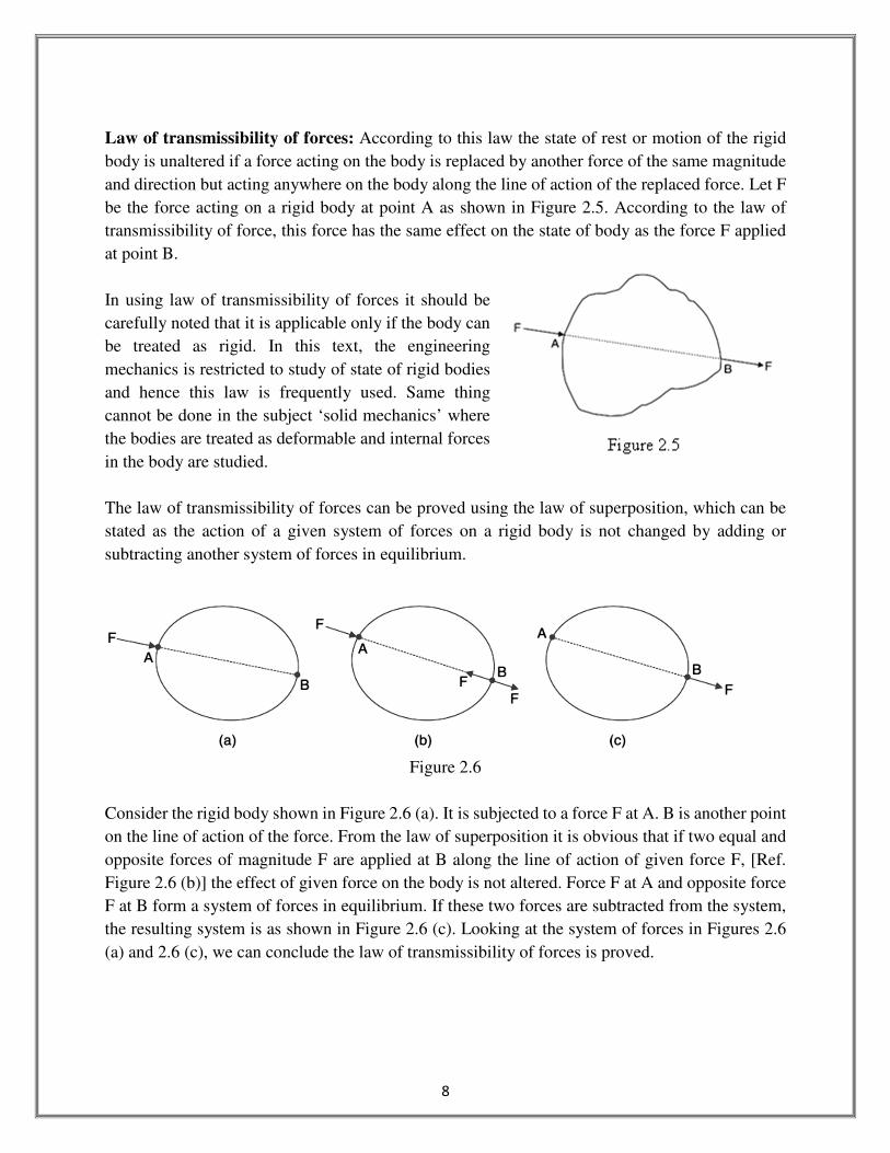
Law of transmissibility of forces: According to this law the state of rest or motion of the rigid

body is unaltered if a force acting on the body is replaced by another force of the same magnitude

and direction but acting anywhere on the body along the line of action of the replaced force. Let F

be the force acting on a rigid body at point A as shown in Figure 2.5. According to the law of

transmissibility of force, this force has the same effect on the state of body as the force F applied

at point B.

In using law of transmissibility of forces it should be

carefully noted that it is applicable only if the body can

be treated as rigid. In this text, the engineering

mechanics is restricted to study of state of rigid bodies

and hence this law is frequently used. Same thing

cannot be done in the subject ‘solid mechanics’ where

the bodies are treated as deformable and internal forces

in the body are studied.

The law of transmissibility of forces can be proved using the law of superposition, which can be

stated as the action of a given system of forces on a rigid body is not changed by adding or

subtracting another system of forces in equilibrium.

Figure 2.6

Consider the rigid body shown in Figure 2.6 (a). It is subjected to a force F at A. B is another point

on the line of action of the force. From the law of superposition it is obvious that if two equal and

opposite forces of magnitude F are applied at B along the line of action of given force F, [Ref.

Figure 2.6 (b)] the effect of given force on the body is not altered. Force F at A and opposite force

F at B form a system of forces in equilibrium. If these two forces are subtracted from the system,

the resulting system is as shown in Figure 2.6 (c). Looking at the system of forces in Figures 2.6

(a) and 2.6 (c), we can conclude the law of transmissibility of forces is proved.

9

Lecture – 3

Parallelogram law of forces: The parallelogram law of forces enables us to determine the single

force called resultant which can replace the two forces acting at a point with the same effect as that

of the two forces. This law was formulated based on experimental results. This law states that if

two forces acting simultaneously on a body at a point are presented in magnitude and

direction by the two adjacent sides of a parallelogram, their resultant is represented in

magnitude and direction by the diagonal of the parallelogram which passes through the point

of intersection of the two sides representing the forces.

In Figure 3.1 the force F1 = 4 units and force F2 = 3 units are acting on a body at point A. Then to

get resultant of these forces parallelogram ABCD is constructed such that AB is equal to 4 units

to linear scale and AC is equal to 3 units. Then according to this law, the diagonal AD represents

the resultant in the direction and magnitude. Thus the resultant of the forces F1 and F2 on the body

is equal to units corresponding to AD in the direction α to F1.

Figure 3.1

Magnitude of Resultant (R)

From C draw CD perpendicular to OA produced.

Let α = Angle between two forces P and Q =∠AOB

Now ∠DAC � ∠DOC (Corresponding angles)

= α

In parallelogram OACB, AC is parallel and equal to OB.

∴ AC � Q

10

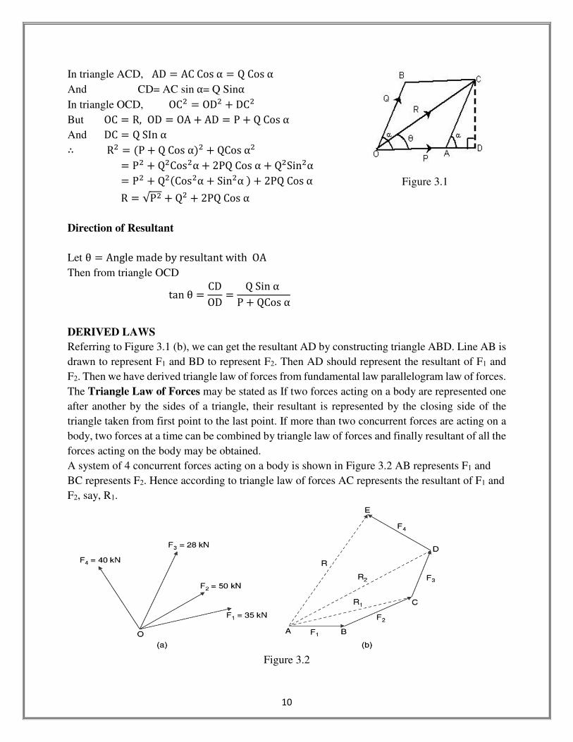
In triangle ACD, AD � ACCosα � QCosα

And CD= AC sinα= Q Sinα

In triangle OCD, OC� � OD� � DC�

But OC � R, OD � OA � AD � P � QCosα And DC � QSInα

∴ R� � �P � QCosα�� � QCosα�

� P� � Q�Cos�α � 2PQCosα � Q�Sin�α

� P� � Q��Cos�α � Sin�α� � 2PQCosα

R � √P� � Q� � 2PQCosα

Direction of Resultant

Let θ � AnglemadebyresultantwithOA

Then from triangle OCD

tanθ � CDOD � QSinα

P � QCosα

DERIVED LAWS

Referring to Figure 3.1 (b), we can get the resultant AD by constructing triangle ABD. Line AB is

drawn to represent F1 and BD to represent F2. Then AD should represent the resultant of F1 and

F2. Then we have derived triangle law of forces from fundamental law parallelogram law of forces.

The Triangle Law of Forces may be stated as If two forces acting on a body are represented one

after another by the sides of a triangle, their resultant is represented by the closing side of the

triangle taken from first point to the last point. If more than two concurrent forces are acting on a

body, two forces at a time can be combined by triangle law of forces and finally resultant of all the

forces acting on the body may be obtained.

A system of 4 concurrent forces acting on a body is shown in Figure 3.2 AB represents F1 and

BC represents F2. Hence according to triangle law of forces AC represents the resultant of F1 and

F2, say, R1.

Figure 3.2

Figure 3.1

11

If CD is drawn to represent F3, then from triangle law of forces AD represents the resultant of R1

and F3. In other words AD represents the resultant of F1, F2 and F3. Let it be called as R2. On the

same line logic can be extended to say that AE represents the resultant of F1, F2, F3 and F4 if DE

represents F4. Thus resultant R is represented by the closing line of the polygon ABCDE in the

direction AE. Thus we have derived polygon of law of forces and it may be stated as ‘If a number

of concurrent forces acting simultaneously on a body are represented in magnitude and direction

by the sides of a polygon, taken in an order, then the resultant is represented in magnitude and

direction by the closing side of the polygon, taken from first point to last point.

Lecture – 4

Composition of forces: If two forces, acting at a point, are represented in magnitude and direction

by the two sides of a parallelogram drawn from one of its angular points, their resultant is

represented both in magnitude and direction by the diagonal of the parallelogram passing through

that angular point

Resultant Force: If two or more forces P, Q, S, act upon a rigid body and if a single force, R, can

be found whose effect upon the body is the same as that of the forces P, Q, S, this single force R

is called the resultant of the other forces.

Resultant of forces acting in the same direction (same straight line) is equal to their sum.

Magnitude and Direction of the Resultant of Two Forces:

Let OA and OB represent the forces P and Q acting at a point O and inclined to each other

at an angle a then the resultant R and direction ‘q’ (shown in figure) will be given by R =

√P2 + Q2 +2PQ cos α and tan θ = Q sinα/P+Q cos α

Figure 4.1

Magnitude and Direction of the Resultant of Two Forces:

Case (i): If P = Q, then tan(θ) = tan (α/2) => θ = α/2

Case (ii): If the forces act at right angles, so that α = 90°,

we have R = √P2+Q2 and tan(θ) = Q/P

12

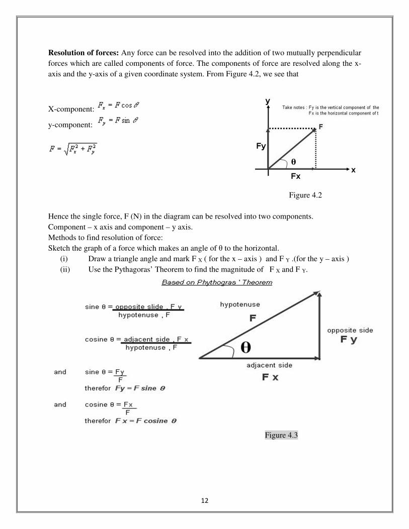
Resolution of forces: Any force can be resolved into the addition of two mutually perpendicular

forces which are called components of force. The components of force are resolved along the x-

axis and the y-axis of a given coordinate system. From Figure 4.2, we see that

X-component:

y-component:

Figure 4.2

Hence the single force, F (N) in the diagram can be resolved into two components.

Component – x axis and component – y axis.

Methods to find resolution of force:

Sketch the graph of a force which makes an angle of θ to the horizontal.

(i) Draw a triangle angle and mark F X ( for the x – axis ) and F Y .(for the y – axis )

(ii) Use the Pythagoras’ Theorem to find the magnitude of F X and F Y.

Figure 4.3

13

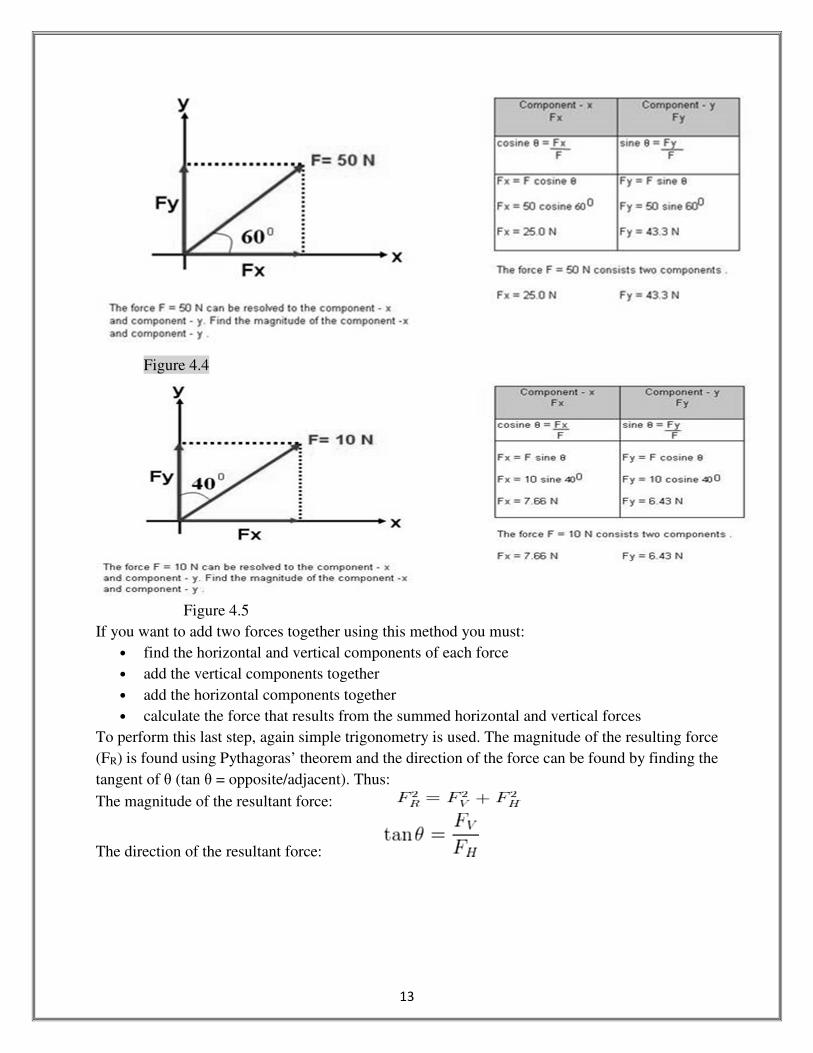
Figure 4.4

Figure 4.5

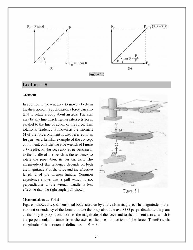
If you want to add two forces together using this method you must:

• find the horizontal and vertical components of each force

• add the vertical components together

• add the horizontal components together

• calculate the force that results from the summed horizontal and vertical forces

To perform this last step, again simple trigonometry is used. The magnitude of the resulting force

(FR) is found using Pythagoras’ theorem and the direction of the force can be found by finding the

tangent of θ (tan θ = opposite/adjacent). Thus:

The magnitude of the resultant force:

The direction of the resultant force:

14

Figure 4.6

Lecture – 5

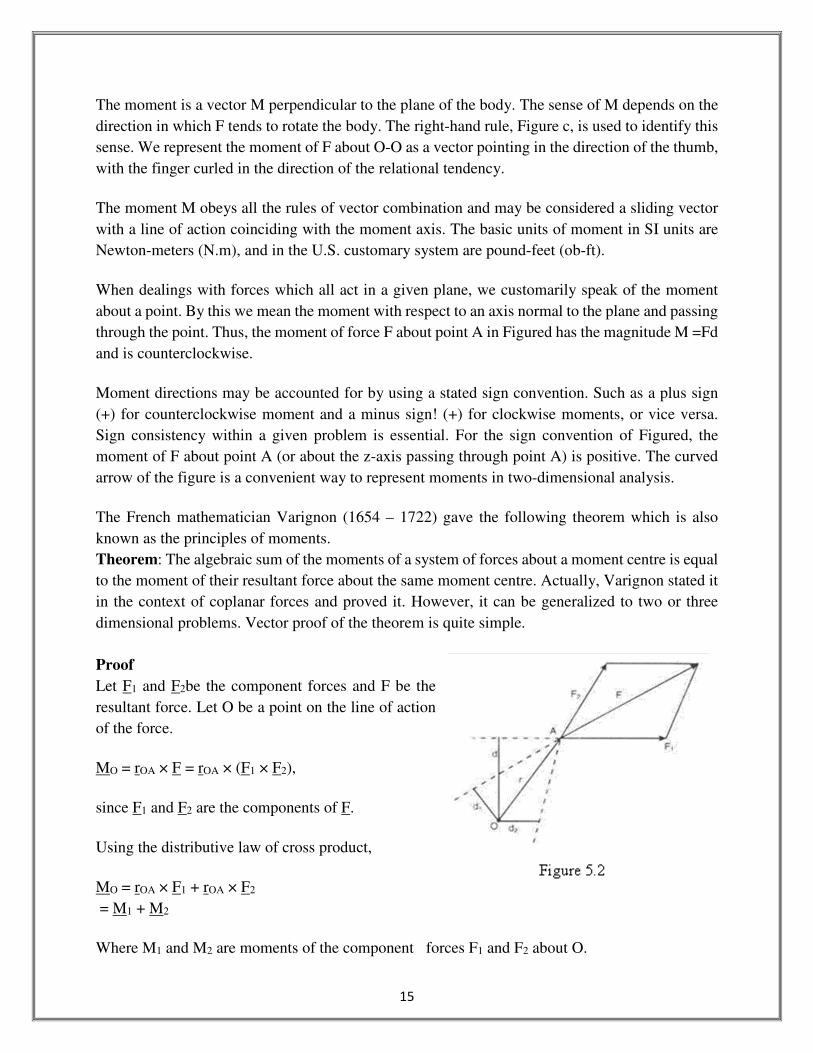
Moment

In addition to the tendency to move a body in

the direction of its application, a force can also

tend to rotate a body about an axis. The axis

may be any line which neither intersects nor is

parallel to the line of action of the force. This

rotational tendency is known as the moment

M of the force. Moment is also referred to as

torque. As a familiar example of the concept

of moment, consider the pipe wrench of Figure

a. One effect of the force applied perpendicular

to the handle of the wench is the tendency to

rotate the pipe about its vertical axis. The

magnitude of this tendency depends on both

the magnitude F of the force and the effective

length d of the wrench handle. Common

experience shows that a pull which is not

perpendicular to the wrench handle is less

effective than the right-angle pull shown.

Moment about a Point

Figure b shows a two-dimensional body acted on by a force F in its plane. The magnitude of the

moment or tendency of the force to rotate the body about the axis O-O perpendicular to the plane

of the body is proportional both to the magnitude of the force and to the moment arm d, which is

the perpendicular distance from the axis to the line of l action of the force. Therefore, the

magnitude of the moment is defined as M � Fd

15

The moment is a vector M perpendicular to the plane of the body. The sense of M depends on the

direction in which F tends to rotate the body. The right-hand rule, Figure c, is used to identify this

sense. We represent the moment of F about O-O as a vector pointing in the direction of the thumb,

with the finger curled in the direction of the relational tendency.

The moment M obeys all the rules of vector combination and may be considered a sliding vector

with a line of action coinciding with the moment axis. The basic units of moment in SI units are

Newton-meters (N.m), and in the U.S. customary system are pound-feet (ob-ft).

When dealings with forces which all act in a given plane, we customarily speak of the moment

about a point. By this we mean the moment with respect to an axis normal to the plane and passing

through the point. Thus, the moment of force F about point A in Figured has the magnitude M =Fd

and is counterclockwise.

Moment directions may be accounted for by using a stated sign convention. Such as a plus sign

(+) for counterclockwise moment and a minus sign! (+) for clockwise moments, or vice versa.

Sign consistency within a given problem is essential. For the sign convention of Figured, the

moment of F about point A (or about the z-axis passing through point A) is positive. The curved

arrow of the figure is a convenient way to represent moments in two-dimensional analysis.

The French mathematician Varignon (1654 – 1722) gave the following theorem which is also

known as the principles of moments.

Theorem: The algebraic sum of the moments of a system of forces about a moment centre is equal

to the moment of their resultant force about the same moment centre. Actually, Varignon stated it

in the context of coplanar forces and proved it. However, it can be generalized to two or three

dimensional problems. Vector proof of the theorem is quite simple.

Proof

Let F1 and F2be the component forces and F be the

resultant force. Let O be a point on the line of action

of the force.

MO = rOA × F = rOA × (F1 × F2),

since F1 and F2 are the components of F.

Using the distributive law of cross product,

MO = rOA × F1 + rOA × F2

= M1 + M2

Where M1 and M2 are moments of the component forces F1 and F2 about O.

16

Lecture - 6

Equilibrium: Equilibrium is the state when all the external forces acting on a rigid body form a

system of forces equivalent to zero. There will be no rotation or translation. The forces are

referred to as balanced.

R1 � 2 F1 � 0R4 � 2 F4 � 0R5 � 2 F5 � 0

FREE BODY DIAGRAM STEPS

1. Determine the free body of interest. (What body is in equilibrium?)

2. Detach the body from the ground and all other bodies (“free” it).

3. Indicate all external forces which include:

- Action on the free body by the supports & connections

- Action on the free body by other bodies

- The weigh effect (=force) of the free body itself (force due to gravity)

4. All forces should be clearly marked with magnitudes and direction. The sense of forces

should be those acting on the body not by the body.

5. Dimensions/angles should be included for moment computations and force computations.

6. Indicate the unknown angles, distances, forces or moments, such as those reactions or

constraining forces where the body is supported or connected. (Text uses hashes on the

unknown forces to distinguish them.)

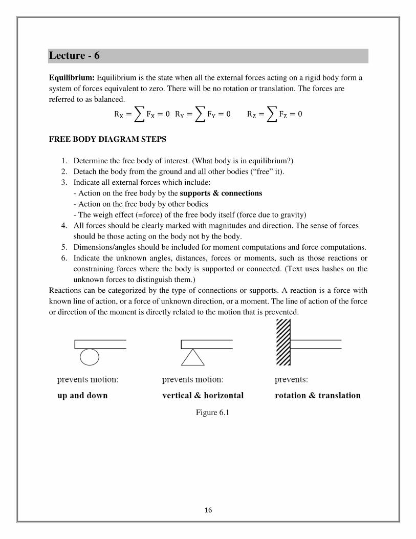
Reactions can be categorized by the type of connections or supports. A reaction is a force with

known line of action, or a force of unknown direction, or a moment. The line of action of the force

or direction of the moment is directly related to the motion that is prevented.

Figure 6.1

17

Table 6.1 Supports for Coplanar Structures

18

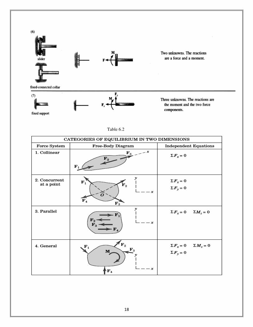
Table 6.2

19

Lecture -7

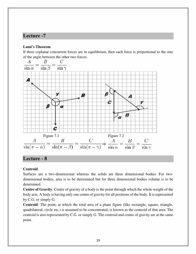
Lami’s Theorem

If three coplanar concurrent forces are in equilibrium, then each force is proportional to the sine

of the angle between the other two forces.

Figure 7.1 Figure 7.2

Lecture - 8

Centroid

Surfaces are a two-dimensional whereas the solids are three dimensional bodies. For two-

dimensional bodies, area is to be determined but for three dimensional bodies volume is to be

determined.

Centre of Gravity: Centre of gravity of a body is the point through which the whole weight of the

body acts. A body is having only one centre of gravity for all positions of the body. It is represented

by C.G. or simply G.

Centroid: The point, at which the total area of a plane figure (like rectangle, square, triangle,

quadrilateral, circle etc.) is assumed to be concentrated, is known as the centroid of that area. The

centroid is also represented by C.G. or simply G. The centroid and centre of gravity are at the same

point.

20

CENTROID OF AN ASSEMBLAGE

The centroid of an assemblage of n similar quantities, ∆7, ∆�, ∆8 … . . ∆; situated at points

P7, P�, P8, … . P; for which the position vectors relative to a selected point О are r7, r�, r8, … . r; has

a position vector r̅ defined as

r = ∑ r>∆>;>?7∑ ∆>;>?7

Where

∆>= i th quantity (for example, this could be an element of length, area, volume, or mass)

r> = position vector of i th element

∑ ∆>;>?7 = sum of all n elements

∑ r>∆>;>?7 = First moment of all elements relative to the selected point O.

In terms of r, y, and z coordinates, the centroid has coordinates

x = ∑ x>∆>;>?7∑ ∆>;>?7

y = ∑ y>∆>;>?7∑ ∆>;>?7

z = ∑ z>∆>;>?7∑ ∆>;>?7

Where

∆>= magnitude of the ith quantity (element)

x, y, z = coordinates of centroid of the assemblage

x>, y>, z>= coordinates of p> at which ∆>, is concentrated.

CENTROID OF A CONTINUOUS QUANTITY

The centroid of a continuous quantity may be located by calculus using infinitesimal elements of

the quantity (such as dL of a line, dA of an area, dV of a volume, or dm of a mass). Thus, for a

mass m we can write

r = C rdmC dm

In terms of r. y, and z coordinates the centroid of the continuous quantity has coordinates

x = C D��C �� = EFG

� y = C H��C �� = EIG

� z = C J��C �� = EIF

�

WhereQHJ, QDJ, QDH= first moments with respect to xy, yz, xz planes.

The centroid of a homogeneous mass coincides with the centroid of its volume.

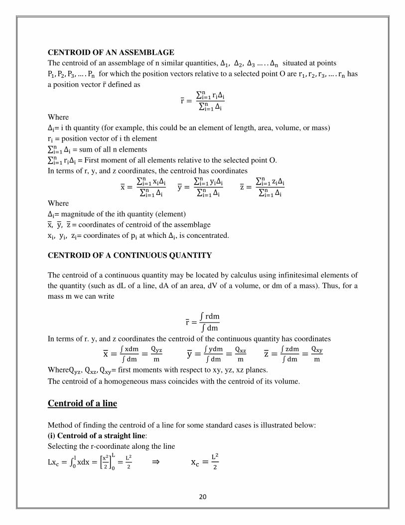
Centroid of a line

Method of finding the centroid of a line for some standard cases is illustrated below:

(i) Centroid of a straight line:

Selecting the r-coordinate along the line

LxL = C xdxMN = OD�

� PNQ = Q�

� ⇒ xL = Q��

21

Thus the centroid lies at midpoint of a straight line, whatever is the orientation of line

Figure 8.1

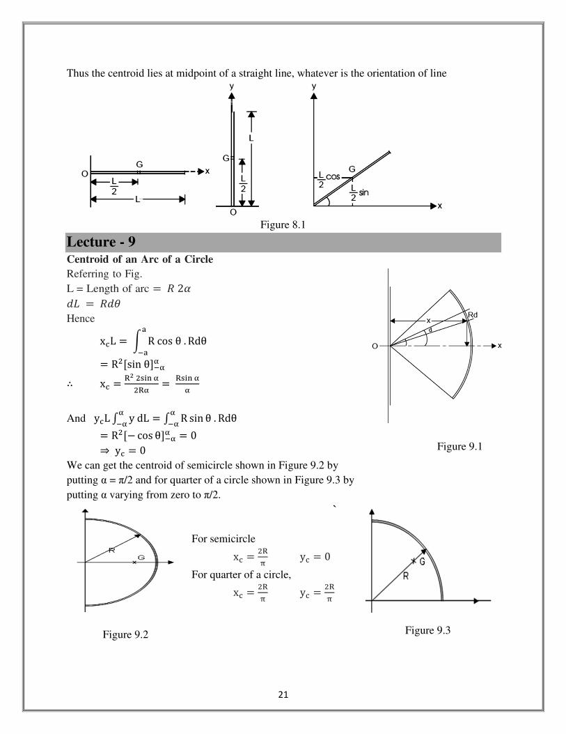
Lecture - 9 Centroid of an Arc of a Circle

Referring to Fig.

L = Length of arc � S2T

UV � SUW

Hence

xLL � X Rcosθ. RdθZ[Z

� R�\sinθ][^^

∴ xL � _��`>;^�_^ � _`>;^

^

And yLL C ydL^[^ � C R sin θ. Rdθ^

[^

� R�\a cos θ][^^ � 0 ⇒ yL � 0

We can get the centroid of semicircle shown in Figure 9.2 by

putting α = π/2 and for quarter of a circle shown in Figure 9.3 by

putting α varying from zero to π/2.

`

For semicircle

xL � �_b yL � 0

For quarter of a circle,

xL � �_b yL � �_

b

Figure 9.1

Figure 9.3

Figure 9.2

22

(iii) Centroid of composite line segments:

The results obtained for standard cases may be used for various segments and then the equations

of the form xLL � ∑ L>x>yLL � ∑ L>y> May be used to get centroid xL and yL . If the line segmets is in space the expression zLL �∑ L>z> may also be used. xL � ∑ cdDd

c , yL � ∑ cdHdc , zL � ∑ cdJd

c ,

Lecture - 10

Difference between Centre of Gravity and Centroid

From the above discussion we can draw the following differences between centre of gravity and

centroid:

(1) The term centre of gravity applies to bodies with weight, and centroid applies to lines, plane

areas and volumes.

(2) Centre of gravity of a body is a point through which the resultant gravitational force (weight)

acts for any orientation of the body whereas centroid is a point in a line plane area volume such

that the moment of area about any axis through that point is zero.

Use of Axis of Symmetry

Centroid of an area lies on the axis of symmetry if it exits. This is useful theorem to locate the

centroid of an area. This theorem can be proved as follows:

Consider the area shown in Figure 10.1. In this figure y-y is the axis of symmetry. The distance

of centroid from this axis is given by: ∑ edDd

e

Consider the two elemental areas shown in Figure 10.1,

which are equal in size and are equidistant from the axis,

but on either side. Now the sum of moments of these areas

cancel each other since the areas and distances are the

same, but signs of distances are opposite. Similarly, we

can go on considering an area on one side of symmetric

axis and corresponding image area on the other side, and

prove that total moments of area about the

symmetric axis is zero. Hence the distance of centroid

from the symmetric axis is zero, i.e. centroid always lies

on symmetric axis.

Making use of the symmetry we can conclude that:

(1) Centroid of a circle is its centre (Figure 10.2);

(2) Centroid of a rectangle of sides’ b and d is at distance b /2 and d/2 from the corner as shown

in Figure 10.3.

Figure 10.1

23

Figure 10.2 Figure 10.3

yf � C H�ee xf � C D�e

e

The location of the centroid using the above equations may be considered as finding centroid

from first principles. Now, let us find centroid of some standard figures from first principles.

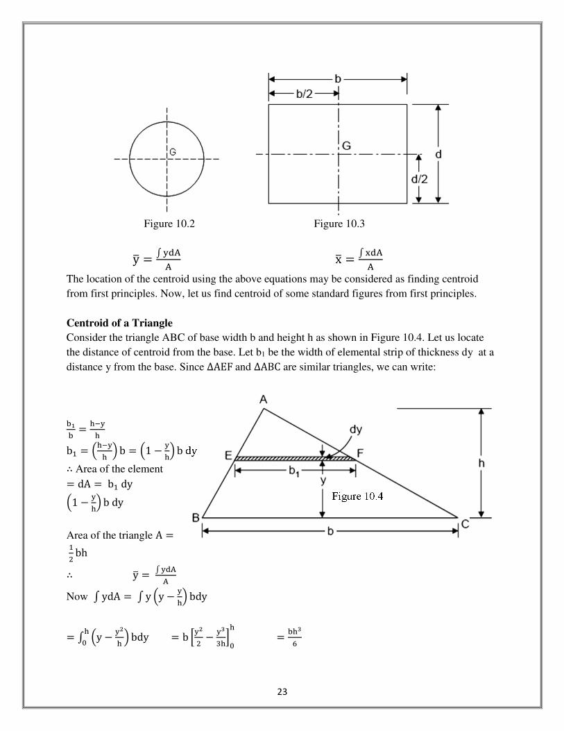
Centroid of a Triangle

Consider the triangle ABC of base width b and height h as shown in Figure 10.4. Let us locate

the distance of centroid from the base. Let b1 be the width of elemental strip of thickness dy at a

distance y from the base. Since ∆AEFand ∆ABC are similar triangles, we can write:

h�h � i[H

i

b7 � ji[Hi k b � j1 a H

ik bdy

∴ Area of the element � dA � b7dy

j1 a Hik bdy

Area of the triangle A �7� bh

∴ yf � C H�ee

Now C ydA � C y jy a Hik bdy

� C jy a H�i k bdyi

N � b OH�� a Hm

8iPNi � him

n

Figure 10.4

24

∴ yf � C H�ee � hi�

n o 7��hi

∴ yf � i8

Thus the centroid of a triangle is at a distance h/3 from the base (or (2/3) h from the apex) of the

triangle where h is the height of the triangle.

Lecture -11

Centroid of a Semicircle

Consider the semicircle of radius R as shown in Figure 11.1. Due to symmetry centroid must lie

on y axis. Let its distance from diametral axis be y. To find y, consider an element at a distance r

from the center O of the semicircle, radial width being dr and bound by radii at θ and θ + dθ.

Area of element � pUWUp

Its moment about diametral axis x is given by: pUW o Up o p sin W � p� sin W UpUW

Total moment of area about diametral axis,

C C R� sin θdrdθ �_N

bN C Oqm

8 PN_b

N sin θ dθ

� _m8 \a cos θ]Nb

_m8 \1 � 1] � �_m

8

Area of semicircle A � 7� πR�

yf st�u;vtwZquZxtvZMZquZ � �ym

m��b_� � z_8b

Thus, the centroid of the circle is at a distance z_8b from the diametral axis.

Centroid of Sector of a Circle

Consider the sector of a circle of angle 2T as shown in Figure. Due to symmetry, centroid lies

on x axis. To find its distance from the center O, consider the elemental area shown.

Area of the element � pUWUp

Its moment about y axis

Figure 11.1

25

� pUθ o dr o r cos θ � p� cos θ UpUθ

Total moment of area about y axis

� C C r� cos θdrdθ_N

^[^

� Oqm8 PN

_ \sin θ][^^

� _m8 2 sin α

Total area of the sector

� C C rdrdθ_N

^[^

� C Oq�� PN

_ dθ^[^

� _�� \θ][^^

� R�α

The distance of centroid from center O

� MomentofareaaboutyaxisAreaofthrfigure

�2R83 Sinα

R�α � 2R3α sin α

Centroid of Parabolic Spandrel

Consider the parabolic spandrel shown in Figure 11.3. Height of the element at a distance r from

O is y = kx2

Width of element = dx

Area of the element = kx2dx

Total area of spandrel =C kx�dxZN

Moment of area about y axis

� X kx�dx o xZN

� X kx8dxZN

� ~kxz4 �

NZ � kaz

4

Moment of area about x axis

Figure 11.2

Figure 11.3

26

� C �eH�� � � C kx�dx �D��

ZN � C ��D�

�Z

N dx � O��D��1� PN

Z � ��Z�7N

∴ xf � �Z�z �Zm

8� � 8Z

z

yf � k�a�4 ka83

� � 3a�10

From the Figure, at x = a, y = h

∴

h = ka�ork � ha�

yf � 310 X h

a� a� = 3h10

Thus, centroid of spandrel is j8Zz , 8i

7Nk

27

Table 11.1 Centroid of Some Common Figures

28

Lecture - 12

Centroid of Composite Sections

So far, the discussion was confined to locating the centroid of simple figures like rectangle,

triangle, circle, semicircle, etc. In engineering practice, use of sections which are built up of many

simple sections is very common. Such sections may be called as built-up sections or composite

sections. To locate the centroid of composite sections, one need not go for the first principle

(method of integration). The given composite section can be split into suitable simple figures and

then the centroid of each simple figure can be found by inspection or using the standard formulae

listed in Table 11.1. Assuming the area of the simple figure as concentrated at its centroid, its

moment about an axis can be found by multiplying the area with distance of its centroid from the

reference axis. After determining moment of each area about reference axis, the distance of

centroid from the axis is obtained by dividing total moment of area by total area of the composite

section.

Composite sections: made up of connected “simpler” shaped parts or holes [rectangle, triangle,

circle, semicircle, etc] Knowing the location of the centroid, C, or center of gravity, G, of the

simpler shaped parts; we can easily determine the location of the C or G for the more complex

composite body

Using the equations:

x � ∑ x>A>∑ A>

y � ∑ y>A>∑ A>

The location of the centroid could be determined [Note: you could replace A with W, M, or L]

Procedures for the Analysis:

Divide the body into parts that are

known shapes.

Holes are considered as parts with

negative weight or size.

Choose an origin and x and y coordinate

system [origin at the left bottom corner

of the shape]

Make a table to summarize the properties of different parts

Using values at the last row of the table find the x and y for the whole section

29

Lecture – 13

THEOREMS OF PAPPUS-GULDINUS

There are two important theorems, first proposed by Greek scientist (about 340 AD) and then

restated by Swiss mathematician Paul Guldinus (1640) for determining the surface area and

volumes generated by rotating a curve and a plane area about a non-intersecting axis, some of

which are shown in Figure 13.1. These theorems are known as Pappus-Guldinus theorems.

Figure 13.1

30

Theorem I

The area of surface generated by revolving a plane curve about a non-intersecting axis in the

plane of the curve is equal to the length of the generating curve times the distance travelled by

the centroid of the curve in the rotation.

Proof: Figure 13.2 shows the isometric view of the plane curve rotated about r-axis by angle W.

We are interested in finding the surface area generated by rotating the curve AB. Let dL be the

elemental length on the curve at D. Its coordinate be y. Then the elemental surface area

generated by this element at D

Figure 13.2

Thus we get area of the surface generated as length of the generating curve times the distance

travelled by the centroid.

Theorem II

The volume of the solid generated by revolving a plane area about a non-intersecting axis in the

plane is equal to the area of the generating plane times the distance travelled by the centroid of

the plane area during the rotation.

Proof: Consider the plane area ABC, which is rotated through an angle θ about r-axis as shown

in Figure 13.3.

Figure 13.3

Let dA be the elemental area of distance y from r-axis. Then the volume generated by this area

during rotation is given by

∴ dV � yθdA

31

V � C yθdA � θ C ydA � θAyL � A�yLθ�

Thus the volume of the solid generated is area times the distance travelled by its centroid during

the rotation. Using Pappus-Guldinus theorems surface area and volumes of cones and spheres

can be calculated as shown below:

(i) Surface area of a cone: Referring to Fig.,

Length of the line generating cone = L

Distance of centroid of the line from the axis of rotation � y � _�

In one revolution centroid moves by distance � 2πy � πR

∴ Surface area = L o�πR� � πRL

(ii) Volume of a cone: Referring to Fig. ,

Area generating solid cone � 7� hR

Centroid G is at a distance y � _8

∴ The distance moved by the centroid in one revolution = 2πy � 2π _8

∴ Volume of solid cone = 7� hR o �b_

8 � b_�i8

(iii) Surface area of sphere: Sphere of radius R is obtained by rotating a semicircular arc of

radius R about its diametral axis. Referring to Fig.,

Length of the arc � πR

Centroid of the arc is at y � �_b from the diametral axis (i.e. axis of rotation)

∴ Distance travelled by centroid of the arc in one revolution= 2πy � 2π �_b � 4R

∴ Surface area of sphere = πR o 4R

(iv) Volume of sphere: Solid sphere of radius R is obtained by rotating a semicircular area about

its diametral axis. Referring to Fig.

Figure 13.4

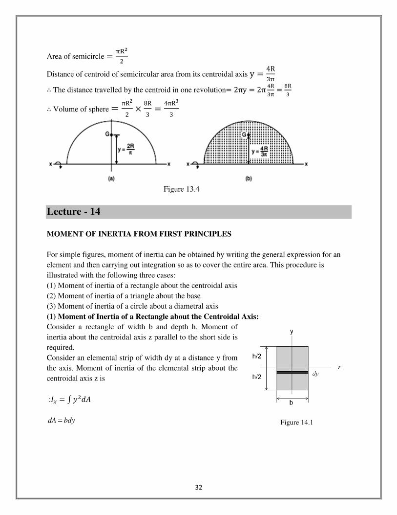
32

Area of semicircle � b_��

Distance of centroid of semicircular area from its centroidal axis y � 4R8b

∴ The distance travelled by the centroid in one revolution= 2πy � 2π z_8b � �_

8

∴ Volume of sphere = πR2

2 o 8R3 = 4πR3

3

Figure 13.4

Lecture - 14

MOMENT OF INERTIA FROM FIRST PRINCIPLES

For simple figures, moment of inertia can be obtained by writing the general expression for an

element and then carrying out integration so as to cover the entire area. This procedure is

illustrated with the following three cases:

(1) Moment of inertia of a rectangle about the centroidal axis

(2) Moment of inertia of a triangle about the base

(3) Moment of inertia of a circle about a diametral axis

(1) Moment of Inertia of a Rectangle about the Centroidal Axis:

Consider a rectangle of width b and depth h. Moment of

inertia about the centroidal axis z parallel to the short side is

required.

Consider an elemental strip of width dy at a distance y from

the axis. Moment of inertia of the elemental strip about the

centroidal axis z is

:�� = C ��U�

bdydA =

Figure 14.1

33

12

883

3

3

33

2

2

3

2

2

2

bh

hhb

yb

bdyyI

h

h

h

h

z

=

−−=

=

=

−

−

∫

(2) Moment of Inertia of a Triangle about its Base: Moment of inertia of a triangle with base

width b and height h is to be determined about the base AB (Figure 14.2). Consider an elemental

strip at a distance y from the base AB. Let dy be the thickness of the strip and dA its area. Width

of this strip is given by:

dyldAdAydI x ==2

For similar triangles

dyh

yhbdA

h

yhbl

h

yh

b

l −=

−=

−=

Integrating dIx from y = 0 to y = h,

( )

h

hh

x

yyh

h

b

dyyhyh

bdy

h

yhbydAyI

0

43

0

32

0

22

43

−=

−=−

== ∫∫∫

12

3bh

I x=

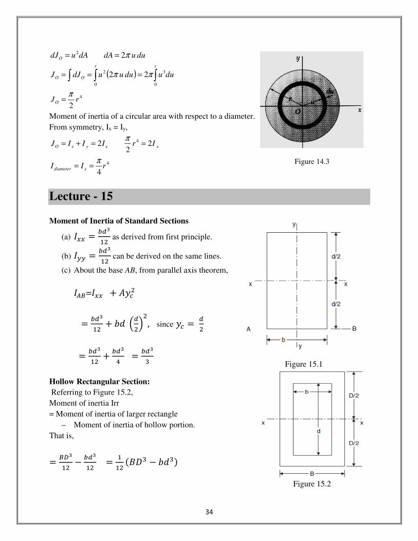
(3) Moment of Inertia of a Circle

Centroidal polar moment of inertia of a circular area by direct integration.

An annular differential area element is chosen,

Figure 14.2

34

Figure 15.2

( ) ∫∫∫ ===

==

rr

OO

O

duuduuudJJ

duudAdAudJ

0

3

0

2

2

22

2

ππ

π

4

2rJO

π=

Moment of inertia of a circular area with respect to a diameter.

From symmetry, Ix = Iy,

xxyxO IrIIIJ 22

2 4==+=

π

4

4rII xdiameter

π==

Lecture - 15

Moment of Inertia of Standard Sections

(a) ��� = ��m7� as derived from first principle.

(b) ��� = ��m7� can be derived on the same lines.

(c) About the base AB, from parallel axis theorem,

���=��� � ����

� ��m7� � �U j�

�k�, since �� � ��

� ��m7� � ��m

z � ��m8

Hollow Rectangular Section:

Referring to Figure 15.2,

Moment of inertia Irr

= Moment of inertia of larger rectangle

– Moment of inertia of hollow portion.

That is,

� ��m7� a ��m

7� � 77� ���8 a �U8�

Figure 14.3

Figure 15.1

35

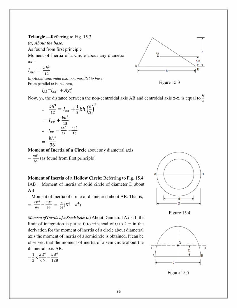
Triangle —Referring to Fig. 15.3.

(a) About the base:

As found from first principle

Moment of Inertia of a Circle about any diametral

axis

��� � ��m7�

(b) About centroidal axis, x-x parallel to base:

From parallel axis theorem, ���=��� � ����

Now, yc, the distance between the non-centroidal axis AB and centroidal axis x-x, is equal to �8

∴ ��m7� = ��� � 7

� �� j�8k�

= ��� � ��m7�

∴ ��� � ��m7� – ��m

7�

� ��836

Moment of Inertia of a Circle about any diametral axis

� ���nz (as found from first principle)

Moment of Inertia of a Hollow Circle: Referring to Fig. 15.4.

IAB = Moment of inertia of solid circle of diameter D about

AB

– Moment of inertia of circle of diameter d about AB. That is,

� ���nz a ���

nz � �64 ��4 a U4�

Moment of Inertia of a Semicircle: (a) About Diametral Axis: If the

limit of integration is put as 0 to �instead of 0 to 2 � in the

derivation for the moment of inertia of a circle about diametral

axis the moment of inertia of a semicircle is obtained. It can be

observed that the moment of inertia of a semicircle about the

diametral axis AB:

� 12 o �Uz

64 � �Uz128

Figure 15.3

Figure 15.4

Figure 15.5

36

(b) About Centroidal Axis x-x:

Now, the distance of centroidal axis �� from the diametral axis is given by:

�� � 4S3� � 2U

3�

And, Area � � 7� o ���

z � ����

From parallel axis theorem,

���=��� � ����

�Uz128 � �   a�U2

8 o ¡2U3�¢2

��� � �Uz128 a Uz

3�

� 0.0068598Uz

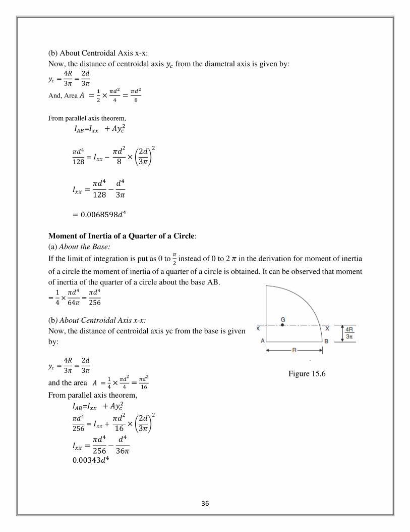
Moment of Inertia of a Quarter of a Circle:

(a) About the Base:

If the limit of integration is put as 0 to ��instead of 0 to 2� in the derivation for moment of inertia

of a circle the moment of inertia of a quarter of a circle is obtained. It can be observed that moment

of inertia of the quarter of a circle about the base AB.

� 14 o �Uz

64� � �Uz256

(b) About Centroidal Axis x-x:

Now, the distance of centroidal axis yc from the base is given

by:

�� � 4S3� � 2U

3�

and the area � � 14 o �U2

4 � �U216

From parallel axis theorem,

���=��� � ����

�Uz256 � �   ��U2

16 o ¡2U3�¢2

��� � �Uz256 a Uz

36�

0.00343Uz

Figure 15.6

37

Table 15.1

38

Lecture - 16

MOMENT OF INERTIA OF COMPOSITE SECTIONS

Beams and columns having composite sections are commonly used in structures. Moment of

inertia of these sections about an axis can be found by the following steps:

(1) Divide the given figure into a number of simple figures.

(2) Locate the centroid of each simple figure by inspection or using standard expressions.

(3) Find the moment of inertia of each simple figure about its centroidal axis. Add the term Ay2

where A is the area of the simple figure and y is the distance of the centroid of the simple figure

from the reference axis. This gives moment of inertia of the simple figure about the reference axis.

(4) Sum up moments of inertia of all simple figures to get the moment of inertia of the composite

section.

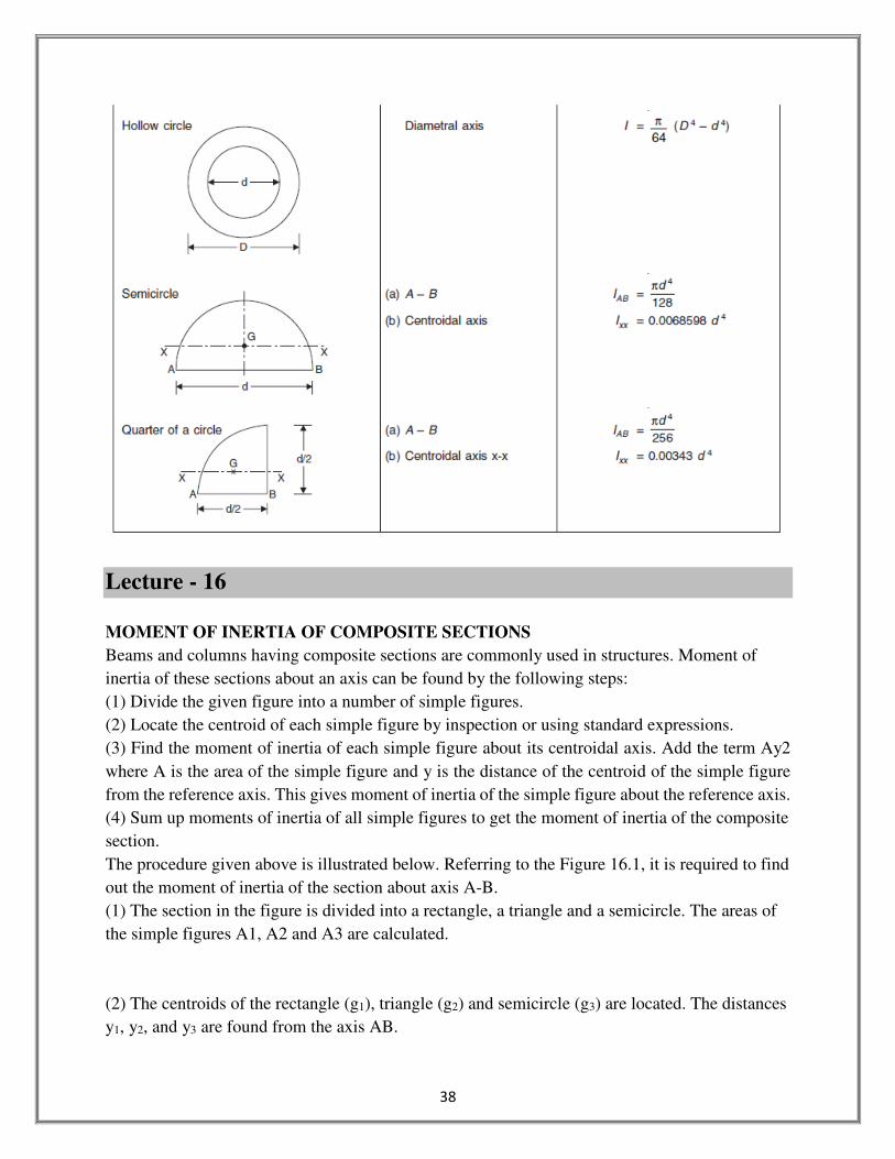
The procedure given above is illustrated below. Referring to the Figure 16.1, it is required to find

out the moment of inertia of the section about axis A-B.

(1) The section in the figure is divided into a rectangle, a triangle and a semicircle. The areas of

the simple figures A1, A2 and A3 are calculated.

(2) The centroids of the rectangle (g1), triangle (g2) and semicircle (g3) are located. The distances

y1, y2, and y3 are found from the axis AB.

39

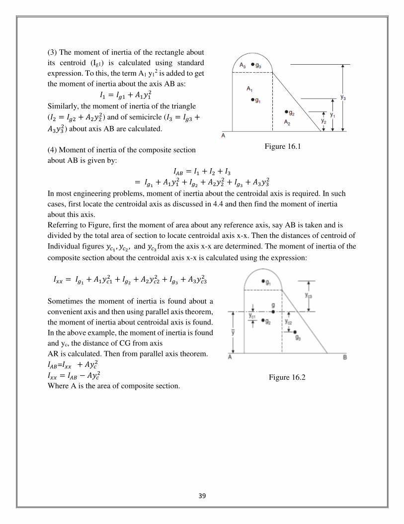
(3) The moment of inertia of the rectangle about

its centroid (Ig1) is calculated using standard

expression. To this, the term A1 y12 is added to get

the moment of inertia about the axis AB as: �7 � �¥7 � �7�7�

Similarly, the moment of inertia of the triangle

(�� � �¥� � �����) and of semicircle (�8 � �¥8 ��8�8�) about axis AB are calculated.

(4) Moment of inertia of the composite section

about AB is given by: ��� � �7 � �� � �8 � �¥� � �7�7� � �¥� � ����� � �¥m � �8�8�

In most engineering problems, moment of inertia about the centroidal axis is required. In such

cases, first locate the centroidal axis as discussed in 4.4 and then find the moment of inertia

about this axis.

Referring to Figure, first the moment of area about any reference axis, say AB is taken and is

divided by the total area of section to locate centroidal axis x-x. Then the distances of centroid of

Individual figures ��� , ��� , and ��mfrom the axis x-x are determined. The moment of inertia of the

composite section about the centroidal axis x-x is calculated using the expression:

��� � �¥� � �7��7� � �¥� � ������ � �¥m � �8��8�

Sometimes the moment of inertia is found about a

convenient axis and then using parallel axis theorem,

the moment of inertia about centroidal axis is found.

In the above example, the moment of inertia is found

and yc, the distance of CG from axis

AR is calculated. Then from parallel axis theorem. ���=��� � ���� ��� � ��� a ����

Where A is the area of composite section.

Figure 16.1

Figure 16.2

40

Lecture - 17

Products of Inertia

For unsymmetrical cross sections (e.g. also for rotated axes) an expression can be determined

denoted as the Product of Inertia: ��� � C  �U� Ixy = 0 if either its x- or y-axis is an axis of symmetry

Figure 17.1

Products of Inertia and rotation of axis

Transfer of axes:

By definition the product of inertia of the area A in Fig.

A/4 with respect to the x- and y-axes in terms of the

coordinnte x0, y0 to the centroidal axes is

��� � X¦ N � U�§ ��N � U��U�

� X  N�NU� � U� X  N U� � U� X �NU�� U�U� X U�

��� � ���ffff � U�U��

(Transfer axis theorem)

Rotation of axes:

��¨ � X � ,� U� � X�� cos W a   sin W�� U�

��¨ � X   ,� U� � X�� sin W a   cos W�� U�

Expanding and substituting in trigonometric identities

©ª«�W � 7[Lt` �¬� ­®©�W � 7¯Lt` �¬

� And the defining relations for ��, �� , ��� give us

Figure 17.1

Figure 17.3

41

��¨ � �� � ��2 � �� a ��2 cos 2W a ��� sin 2W ��¨ � �� � ��2 a �� a ��2 cos 2W a ��� sin 2W

Lecture - 18

FRICTION

When a body moves or tends to move on another body, a force appears between the surfaces. This

force is called force of friction and it acts opposite to the direction of motion. Its line of action is

tangential to the contacting surfaces. The magnitude of this force depends on the roughness of

surfaces.

In engineering applications friction is desirable and undesirable. We can walk on the ground

because of friction. Friction is useful in power transmission by belts. It is useful in appliances like

brakes, bolts, screw jack, etc. It is undesirable in bearing and moving machine parts where it results

in loss of energy and, thereby, reduces efficiency of the machine.

TYPES OF FRICTION

There are two types of friction:

(a) Friction in un-lubricated surfaces or dry surfaces, and

(b) Friction in lubricate surfaces.

The friction that exists when one dry surface slides over another dry surface is known as dry

friction and the friction.

If between the two surfaces a thick layer of an oil or lubricant is introduced, a film of such

lubrication is formed on both the surfaces. When a surface moves on the other, in effect, it is one

layer of oil moving on the other and there is no direct contact between the surfaces. The friction is

greatly reduced and is known as film friction.

LAWS OF DRY FRICTION

The laws of dry friction, are based on experimental evidences, and as such they are empirical in

nature:

(a) The friction force is directly proportional to the normal reaction between the surfaces.

(b) The frictional force opposes the motion or its tendency to the motion.

(c) The frictional force depends upon the nature of the surfaces in contact.

(d) The frictional force is independent of the area and the shape of the contacting surfaces.

(e) For moderate speeds, frictional force is independent of the relative velocities of the bodies in

contact.

42

STATIC AND KINETIC FRICTION

Suppose a block of weight W rests on a plane surface as shown in Figure 18.1. The surface offers

a normal reaction RN equal to the weight W. Suppose, now, a pull P1 is applied to the block such

that it actually does not move but instead tends to move. This will be opposed by frictional force

F1, equal to P1. The resultant reaction will be R1 Friction inclined at an angle °1 with the normal

reaction. If the pull is increased to P2, the frictional force will increase to F2 and the resultant

reaction will increase to R2 inclined at an angle of ° 2. Thus, with increase of the pull or attractive

force, the frictional force; the resultant reaction and its inclination will increase.

Figure 18.1 shows a block of mass m

resting on a plane surface with application

of force P1, P2 and P3 at which the body

impends sliding, the self-adjusting

frictional forces will increase from F1, to

F2 and finally F3 when the body tends to

move. Thus, in the limiting condition, the

resultant active force will be R and

reactive force RR.

The frictional resistance offered so

long as the body does not move, is

known as static friction. F1 and F2 are

the static frictional forces. It may be

noted that the direction of the resultant

reaction RR is such that it opposes the

motion.

The ultimate value of static friction (F)

when the body just tends to move is

called limiting friction or maximum

static friction or friction of impending

slide. The condition, when all the

forces are just in equilibrium and the

body has a tendency to move, is called limiting equilibrium position. When a body moves relative

to another body, the resisting force between them is called kinetic or sliding friction. It has been

experimentally found that the kinetic friction is less than the maximum static friction.

COEFFICIENT OF FRICTION

The ratio between the maximum static frictional force and the normal reaction RN remains

constant which is known as coefficient of static friction denoted by Greek letter μ.

Coefficientoffriction � sZD>�²�`vZv>Lwq>Lv>t;ZMwtqLu³tq�ZMquZLv>t; μ � ´

_µ

The maximum angle ϕ which the resultant reaction R makes with the normal reaction RN is known

as angle of friction. It is denoted by ϕ.

Figure 18.1

43

Figure 18.2

tan ϕ � ´_µ ⇒ ϕ � tan[7 μ

The coefficient of friction is different for different substances and even varies for different

conditions of the same two surfaces.

ANGLE OF REPOSE

Consider a mass m resting on an inclined plane. If the angle of inclination is slowly increased, a

stage will come when the block of mass m will tend to slide down (Figure 18.2). This angle of the

plane with horizontal plane is known as angle of repose. For satisfying the conditions of

equilibrium all the forces are resolved parallel to the plane and perpendicular to it.

P� S·¸ª«T ¹º � S·¸ª«T Pmg � tanα

But »

�¼ � ´_µ � μ � tanϕ

⇒ tanα � tanϕ

Angleofreposeα � Angleoffrictionϕ

Lecture - 19

LEAST FORCE REQUIRED TO DRAG A BODY ON A ROUGH HORIZONTAL PLANE

Suppose a block, of mass m, is placed on a

horizontal rough surface as shown in

Figure 19.1 and an attractive force P is

applied at an angle θ with the horizontal

such that the block just tends to move.

For satisfying the equilibrium conditions

the forces are resolved vertically and

horizontally.

For ∑ V � 0 mg a Psinθ � R³

Figure 19.1

44

Or R³ � �mg a P sin θ�

For ∑ H � 0 P cos θ � F � μR; � μ�mg a P sin θ�

SubstitutingthevalueofR³P cos θ � sin ϕcos ϕ �mg a P sin θ�

P cos θcos ϕ � mg sin ϕ a P sin θ sin ϕ

P cos θcos ϕ � P sin θ sin ϕ � mg sin ϕ

P�cos θcos ϕ � sin θ sin ϕ� � mg sin ϕ

P cos�θ a ϕ� � mg sin ϕ ⇒ P � �¼ `>; ¿Lt`�À[¿�

For P to be least, the denominator cos�θ a ϕ� must be maximum and it will be so if cos�θ a ϕ� � 1 or θ a ϕ � 0 ⇒ θ � ϕforleastvalueofP ⇒ PMuZ`v � mg sin ϕ

Hence, the force P wiI1 be the least if angle of its inclination with the horizontal: θ is equal to the

angle of friction ϕ.

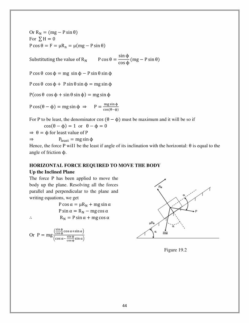
HORIZONTAL FORCE REQUIRED TO MOVE THE BODY

Up the Inclined Plane

The force P has been applied to move the

body up the plane. Resolving all the forces

parallel and perpendicular to the plane and

writing equations, we get P cos α � μR³ � mg sin α P sin α � R³ a mg cos α ∴ R³ = P sin α � mg cos α

Or P � mg jÁd ÃÄÅÁ à Lt` ^¯`>; ^kjLt` ^[Ád ÃÄÅÁ à `>; ^k

Figure 19.2

45

� mg �sin ϕ cos α � sinα cos ϕ��cos α cos ϕ a sin ϕ sin α� � mg sin�α � ϕ�cos�α � ϕ� � mg tan�α � ϕ�

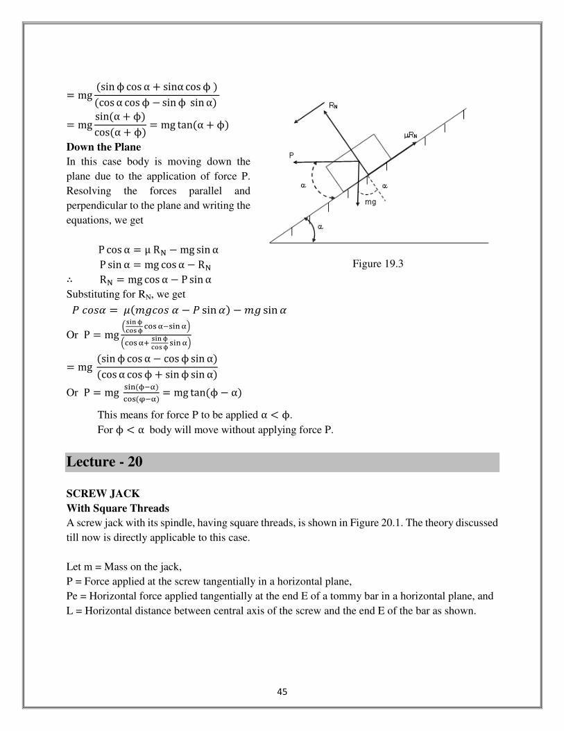
Down the Plane

In this case body is moving down the

plane due to the application of force P.

Resolving the forces parallel and

perpendicular to the plane and writing the

equations, we get

P cos α � μR³ a mg sin α P sin α � mg cos α a R³ ∴ R³ = mg cos α a P sin α

Substituting for RN, we get

Æ­®©T � Ç�¹º­®©T a Æ sin T� a ¹º sin T

Or P � mg jÁd ÃÄÅÁ à Lt` ^[`>; ^kjLt` ^¯Ád ÃÄÅÁ à `>; ^k

� mg �sin ϕ cos α a cos ϕ sin α��cos α cos ϕ � sin ϕ sin α�

Or P � mg `>;�¿[^�Lt`�È[^� � mg tan�ϕ a α�

This means for force P to be applied α < ϕ.

For ϕ < α body will move without applying force P.

Lecture - 20

SCREW JACK

With Square Threads

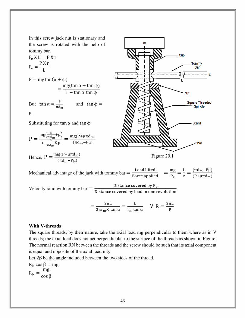
A screw jack with its spindle, having square threads, is shown in Figure 20.1. The theory discussed

till now is directly applicable to this case.

Let m = Mass on the jack,

P = Force applied at the screw tangentially in a horizontal plane,

Pe = Horizontal force applied tangentially at the end E of a tommy bar in a horizontal plane, and

L = Horizontal distance between central axis of the screw and the end E of the bar as shown.

Figure 19.3

46

In this screw jack nut is stationary and

the screw is rotated with the help of

tommy bar. PuXL � PXr

Pu � PXrL

P � mg tan�α � ϕ�� mg�tan α � tan ϕ�

1 a tan αtan ϕ

But tan α � »b�Ê and tan ϕ �

μ

Substituting for tan α and tan ϕ

P � �¼j ËÌÍʯÎk7[ ÏÌÍÊ1Î � �¼�»¯Îb�Ê�

�b�Ê[»Î�

Hence, P � �¼�»¯Îb�Ê��b�Ê[»Î�

Mechanical advantage of the jack with tommy bar � QtZ�M>wvu�´tqLuZÐÐM>u� � �¼

»Ñ � Qq � �b�Ê[»Î�

�»¯Îb�Ê�

Velocity ratio with tommy bar:� Ò>`vZ;LuLtÓuqu�hH»ÑÒ>`vZ;LuLtÓuqu�hHMtZ�>;t;uquÓtM²v>t;

� �bQ�bqÊ1 vZ; ^ � Q

qÊ vZ; ^ V. R � �bQ»

With V-threads

The square threads, by their nature, take the axial load mg perpendicular to them where as in V

threads; the axial load does not act perpendicular to the surface of the threads as shown in Figure.

The normal reaction RN between the threads and the screw should be such that its axial component

is equal and opposite of the axial load mg.

Let 2β be the angle included between the two sides of the thread. R³ cos β � mg

R³ � mgcos β

Figure 20.1

47

Frictional force which acts tangential to the surface of the

threads � μR³ � Î�¼Lt` Õ � μ7mg

where μ7may be regarded as virtual coefficient of

friction:

⇒ μ7 � ÎLt` Õ

While treating V-threads for finding out effort F or ‘e’,

etc. μ may be substituting by μ7 in all the relevant

equations meant for the square threads.

It may be observed that force required to lift a given load

with V-threads will be more than that with square

threads.

Screw threads are also used for transmission of power

such as in lathes (lead screw), milling machines, etc. The

square threads will transmit power without any side thrust

but is difficult to cut. The Acme threads, though not as

efficient as the square threads are easier to cut.

Lecture – 21

Belt Friction

Belts are small strips that tightly wrap around objects and hold the objects firmly. They are used

in simple machines to transfer torque from one shaft to another. Very often, the diameters of the

Figure 20.2

Figure 21.1

48

two shafts are so different that some reduction or enhancement of the rotational speed is also

achieved during transmission.

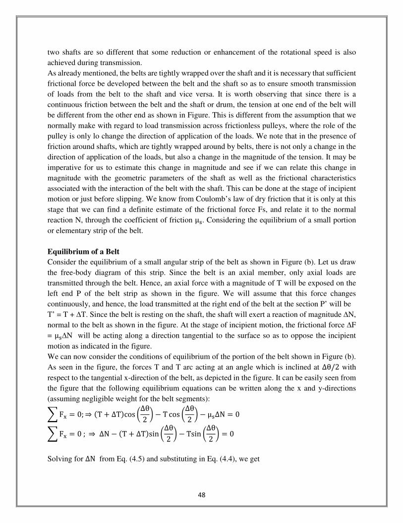
As already mentioned, the belts are tightly wrapped over the shaft and it is necessary that sufficient

frictional force be developed between the belt and the shaft so as to ensure smooth transmission

of loads from the belt to the shaft and vice versa. It is worth observing that since there is a

continuous friction between the belt and the shaft or drum, the tension at one end of the belt will

be different from the other end as shown in Figure. This is different from the assumption that we

normally make with regard to load transmission across frictionless pulleys, where the role of the

pulley is only lo change the direction of application of the loads. We note that in the presence of

friction around shafts, which are tightly wrapped around by belts, there is not only a change in the

direction of application of the loads, but also a change in the magnitude of the tension. It may be

imperative for us to estimate this change in magnitude and see if we can relate this change in

magnitude with the geometric parameters of the shaft as well as the frictional characteristics

associated with the interaction of the belt with the shaft. This can be done at the stage of incipient

motion or just before slipping. We know from Coulomb’s law of dry friction that it is only at this

stage that we can find a definite estimate of the frictional force Fs, and relate it to the normal

reaction N, through the coefficient of friction μ`. Considering the equilibrium of a small portion

or elementary strip of the belt.

Equilibrium of a Belt

Consider the equilibrium of a small angular strip of the belt as shown in Figure (b). Let us draw

the free-body diagram of this strip. Since the belt is an axial member, only axial loads are

transmitted through the belt. Hence, an axial force with a magnitude of T will be exposed on the

left end P of the belt strip as shown in the figure. We will assume that this force changes

continuously, and hence, the load transmitted at the right end of the belt at the section P’ will be

T’ = T + ∆T. Since the belt is resting on the shaft, the shaft will exert a reaction of magnitude ∆N,

normal to the belt as shown in the figure. At the stage of incipient motion, the frictional force ∆F

= μ`∆N will be acting along a direction tangential to the surface so as to oppose the incipient

motion as indicated in the figure.

We can now consider the conditions of equilibrium of the portion of the belt shown in Figure (b).

As seen in the figure, the forces T and T arc acting at an angle which is inclined at ∆θ/2 with

respect to the tangential x-direction of the belt, as depicted in the figure. It can be easily seen from

the figure that the following equilibrium equations can be written along the x and y-directions

(assuming negligible weight for the belt segments):

2 FD = 0; ⇒ �T + ΔT�cos Ú∆θ2 Û − T cos Ú∆θ

2 Û − μ`∆N = 0

2 FD = 0 ; ⇒ ΔN − �T � ΔT�sin Ú∆θ2 Û − Tsin Ú∆θ

2 Û = 0

Solving for ΔN from Eq. (4.5) and substituting in Eq. (4.4), we get

49

ΔTcos Ú∆θ2 Û − μ`�2T + ΔT�sin Ú∆θ

2 Û = 0

Dividing Eq. (4.6) by ∆θ and by rearranging the terms, we obtain

∆T∆θ cos Ú∆θ

2 Û − μ` ÚT + ΔT2 Û

sin j∆θ2 k

j∆θ2 k

= 0

We now take the limit as ∆W → 0 in Eq. (4.7). Noting that this implies that ­®© �∆W/2� → 1.

Þßà j∆á� k

j∆á� k → 1, and that ∆â is very small compared to T so that we can replace the incremental

operator with a differential operator. Hence, we find

UâUW − ÇÞâ = 0 ⇒ Uâ

â = ÇÞUW

Equation can be integrated between the limits of the variables concerned. We recognize that the

tension T varies from a value of T1 at the left side of the belt to a value of T2 at the right side of

the belt around the shaft. The angle of wrap ranges from O at the left end of the wrap to a value of

ã at the right end of the wrap. Hence, we can write

X Uââ

ä�

ä�= ÇÞ X UW

å

N⇒ æ« Úâ�

â7Û = ÇÞã

Using above equation, we can obtain a relation between the tensions at the two ends of the belt, as

given by the relation

T� = T7eÎÁÕ

Equation gives us a simple expression that will help us estimate the tension in a belt for a given

wrap angle β, or will help us determine the wrap angle that is necessary for a given tension in the

belt and a given surface friction coefficient μ`. Above equation can also be used to solve for the

tension that is required to arrest motion in a band brake. A band brake is a simple braking

mechanism, where a belt is brought in contact with a rotating shaft and the friction between the

shaft and the belt is utilized to arrest the rotation of the shaft. In such systems, it is imperative to

ensure that there is sufficient wrap angle between the belt and the shaft to ensure that enough

frictional force is developed between the shaft and the belt so that incipient motion can be arrested.

Above equation will be useful to make an estimate of these conditions.

50

Lecture - 22

Single-purchase crab winch

The machine as shown in Fig. 22.1, comprises of an effort axle which carries a smaller gear

wheel called the pinion and a load axle which carries a larger gear wheel called the spur wheel.

The gears of the two wheels are meshed together. Both axles which are capable of rotation are

mounted in suitable bearings in a rigid frame. A rope wound round the load axle carries the load

W. The effort is applied at the end of the lever. This rotates the pinion and the spur wheel so that

the load is lifted up. Distance moved by thy effort in one revolution= 2πL . The pinion also

makes one revolution in this process but the spur wheel and the load axle make T1/T2 of one

revolution.

Hence the distance moved by the load=π DT1/T2.

V. R = Distance moved by effortDistance Moved by load 2πL

OπDT7 T�ç P= 2LT�

DT7

MA = WP and η = MA

VR = WDT72PLT�

Where T7 = number of teeth on the pinion,

T2 = number of teeth on the spur wheel,

D= diameter of the load axle and

L = lever arm of the applied effort.

Figure 22.1

Double-purchase crab winch

Use of two pairs of gear wheels gives a greater velocity ratio to a double-purchase crab winch in

comparison to a single-purchase machine. There are two pinions and two spur wheels. The pinion

51

of the effort axle which is rotated by the lever, meshes with the spur wheel of an intermediate axle.

This axle carries on it another pinion that meshes with the spur wheel of the load axle. The rotation

of the load axle winds the rope and lifts the load up as shown in fig.

For one revolution of the effort lever, distance moved by the effort = 2πL.

No. of revolutions made by pinion of effort axle = 1.

No. of revolutions made by spur wheel and pinion of intermediate axle = T1/T2.

No. of revolutions made by spur wheel and axle of the load axle = x�x�

X xmx�

Distance moved by the load = πD X x�x�

X xmx�

.

VR = Distance moved by effortDistance moved by load

= 2πLπDT7T8

X T�Tz = 2LT�TzDT7T8

M. R = WP

And η = seê_ = cÒx�xm

�Q»x�x�

Where T1 — number of teeth on the pinion of the effort axle,

T2 = number of teeth on the spur wheel of intermediate axle,

T3 = number of teeth on the pinion of the intermediate axle,

T4 — number of teeth on the spur wheel of the load axle,

D — diameter of load axle,

And L — lever arm of the applied effort.

Lecture - 23

Wedge and Block Friction

Wedge is the oldest type of simple machine used to raise large loads like stone blocks, steel

columns, etc. i.e. by pushing a wedge with considerably smaller force, larger weights can be raised

or lifted. Due to friction, properly angled wedge (triangular or trapezoidal) does not get displaced,

hence used widely in civil and mechanical engineering applications.

There are many other applications of friction also, but in case of wedges we obtain coplanar

concurrent force system in equilibrium. By drawing free body diagram with proper direction of

force of friction, problems can be solved. One illustration of F.B.D. of wedge is shown below.

This can be extended to connected blocks also.

52

Figure 23.1

Lecture - 24

SIMPLE MACHINES

A machine is a contrivance by means of which a given resistance or load is overcome or lifted by

applying a force of suitable magnitude, direction, sense or line of action or a combination of these.

In olden days. Animal power and/or raw human effort were used to lift or drag heavy loads.

BASIC MACHINES

With the invention of simple machines like lever, inclined plane, and pulley the magnitude of effort

required to lift heavy loads is reduced as is obvious in Figure (a), (b), (c). Figure (a) shows a lever,

through which a load W is being lifted by a smaller effort P. By applying the principle of moments

about the fulcrum F,

53

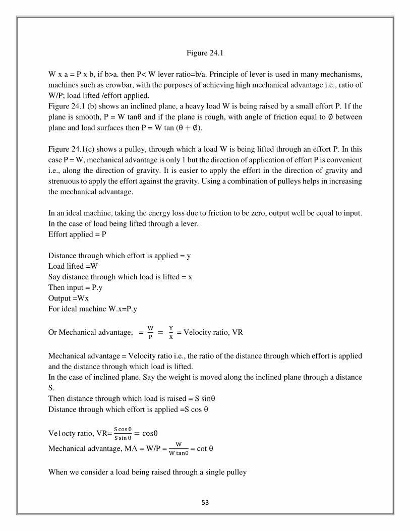
Figure 24.1

W x a = P x b, if b>a. then P< W lever ratio=b/a. Principle of lever is used in many mechanisms,

machines such as crowbar, with the purposes of achieving high mechanical advantage i.e., ratio of

W/P; load lifted /effort applied.

Figure 24.1 (b) shows an inclined plane, a heavy load W is being raised by a small effort P. 1f the

plane is smooth, P = W tanθ and if the plane is rough, with angle of friction equal to ∅ between

plane and load surfaces then P = W tan (θ � ∅).

Figure 24.1(c) shows a pulley, through which a load W is being lifted through an effort P. In this

case P = W, mechanical advantage is only 1 but the direction of application of effort P is convenient

i.e., along the direction of gravity. It is easier to apply the effort in the direction of gravity and

strenuous to apply the effort against the gravity. Using a combination of pulleys helps in increasing

the mechanical advantage.

In an ideal machine, taking the energy loss due to friction to be zero, output well be equal to input.

In the case of load being lifted through a lever.

Effort applied = P

Distance through which effort is applied = y

Load lifted =W

Say distance through which load is lifted = x

Then input = P.y

Output =Wx

For ideal machine W.x=P.y

Or Mechanical advantage, = c» = 4

1 = Velocity ratio, VR

Mechanical advantage = Velocity ratio i.e., the ratio of the distance through which effort is applied

and the distance through which load is lifted.

In the case of inclined plane. Say the weight is moved along the inclined plane through a distance

S.

Then distance through which load is raised = S sinθ

Distance through which effort is applied =S cos θ

Ve1octy ratio, VR= ì Lt` Àì `>; À = cosθ

Mechanical advantage, MA = W/P = c

c vZ;À = cot θ

When we consider a load being raised through a single pulley

54

Distance through which load is lifted = x

Distance through which effort is applied = y

But x = y

Velocity ratio, y/x = 1

Mechanical advantage. = W / P =1

REVERSIBILITY OF A MACHINE

A simple pulley, as a simple machine, is a fully reversible machine. Let an effort P be required to

lift a load W. If the effort P is removed the load W falls or moves in the reverse direction. Thus, a

simple pulley is a reversible machine. If the load being lifted does not move in the reverse direction

on removable of the effort, then the machine is non-reversible or self-locking. Thus, a machine,

will be reversible if the work done by the load is equal to or more, than the frictional work.

Let W be the resistance or load moving through a distance d, and P be the applied effort which

moves through a distance d.

P be the applied effort which moves through a distance D.

Then Work input = PD.

Work output = Wd.

:. Work lost in friction= (work input — work output)

= (PD – Wd).

For a reversible machine, when effort is zero

The output should be > frictional losses

Or, Wd ≥ �PD − Wd�

Or, 2Wd ≥ PD

∴ c�»Ò ≥ 7

�

Or, η ≥ 7�

For a reversible machine.

That is, a machine will be reversible if its efficiency is equal to or more than 50%