1 TT. Liu, BE280A, UCSD Fall 2012 Bioengineering 280A Principles of Biomedical Imaging Fall Quarter 2012 MRI Lecture 4 TT. Liu, BE280A, UCSD Fall 2012 MTF = Fourier Transform of Impulse Response Bushberg et al 2001 TT. Liu, BE280A, UCSD Fall 2012 Modulation Transfer Function (MTF) or Frequency Response Bushberg et al 2001 TT. Liu, BE280A, UCSD Fall 2012 Modulation Transfer Function Bushberg et al 2001

Welcome message from author
This document is posted to help you gain knowledge. Please leave a comment to let me know what you think about it! Share it to your friends and learn new things together.
Transcript
1
TT. Liu, BE280A, UCSD Fall 2012
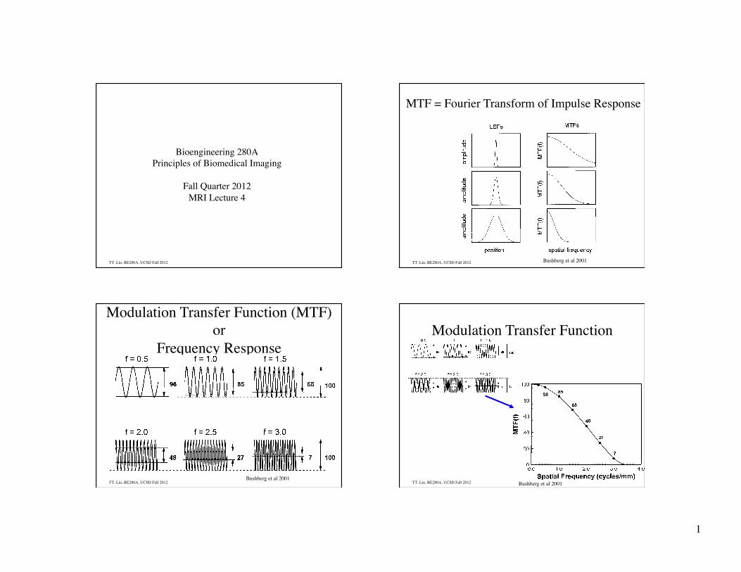
Bioengineering 280A ���Principles of Biomedical Imaging���
���Fall Quarter 2012���
MRI Lecture 4���
TT. Liu, BE280A, UCSD Fall 2012
MTF = Fourier Transform of Impulse Response
Bushberg et al 2001
TT. Liu, BE280A, UCSD Fall 2012
Modulation Transfer Function (MTF) or���
Frequency Response
Bushberg et al 2001 TT. Liu, BE280A, UCSD Fall 2012
Modulation Transfer Function
Bushberg et al 2001

2
TT. Liu, BE280A, UCSD Fall 2012 TT. Liu, BE280A, UCSD Fall 2012
Eigenfunctions
€
z(x) = g(x)∗e j2πkxx
= g(u)−∞
∞
∫ e j2πkx (x−u)du
=G(kx )ej2πkxx
The fundamental nature of the convolution theorem may be better understood by observing that the complex exponentials are eigenfunctions of the convolution operator.
g(x) z(x)
€
e j2πkxx
The response of a linear shift invariant system to a complex exponential is simply the exponential multiplied by the FT of the system’s impulse response.
TT. Liu, BE280A, UCSD Fall 2012
Convolution/Multiplication
€
h(x) = H(kx−∞
∞
∫ )e j 2πkxxdkx
Now consider an arbitrary input h(x).
h(x) g(x) z(x)
Recall that we can express h(x) as the integral of weighted complex exponentials.
Each of these exponentials is weighted by G(kx) so that the response may be written as
€
z(x) = G(kx )H(kx−∞
∞
∫ )e j2πkxxdkx
TT. Liu, BE280A, UCSD Fall 2012
Convolution/Modulation Theorem
€
F g(x)∗ h(x){ } = g(u)∗ h(x − u)du−∞
∞
∫[ ]e− j 2πkxx−∞
∞
∫ dx
= g(u) h(x − u)−∞
∞
∫ e− j2πkxx−∞
∞
∫ dxdu
= g(u)H(kx )e− j2πkxu
−∞
∞
∫ du
=G(kx )H(kx )
Convolution in the spatial domain transforms into multiplication in the frequency domain. Dual is modulation
€
F g(x)h(x){ } =G kx( )∗H(kx )
3
TT. Liu, BE280A, UCSD Fall 2012
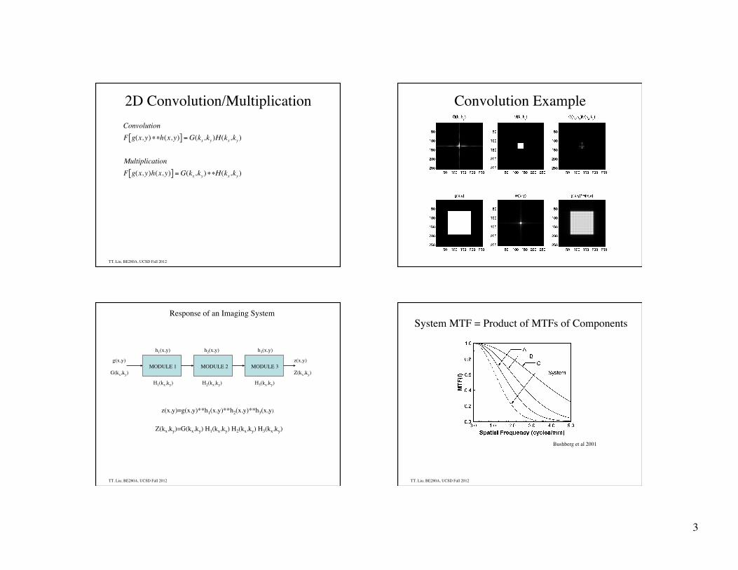
2D Convolution/Multiplication
€
ConvolutionF g(x,y)∗∗h(x,y)[ ] =G(kx,ky )H(kx,ky )
MultiplicationF g(x,y)h(x,y)[ ] =G(kx,ky )∗∗H(kx,ky )
TT. Liu, BE280A, UCSD Fall 2012
Convolution Example
TT. Liu, BE280A, UCSD Fall 2012
Response of an Imaging System
G(kx,ky) H1(kx,ky) H2(kx,ky) H3(kx,ky)
g(x,y)
h1(x,y) h2(x,y) h3(x,y)
MODULE 1 MODULE 2 MODULE 3 z(x,y)
Z(kx,ky)
Z(kx,ky)=G(kx,ky) H1(kx,ky) H2(kx,ky) H3(kx,ky)
z(x,y)=g(x,y)**h1(x,y)**h2(x,y)**h3(x,y)
TT. Liu, BE280A, UCSD Fall 2012
System MTF = Product of MTFs of Components
Bushberg et al 2001

4
TT. Liu, BE280A, UCSD Fall 2012
Useful Approximation
€
FWHMSystem = FWHM12 +FWHM2
2 +FWHMN2
ExampleFWHM1 =1mmFWHM2 = 2mm
FWHMsystem = 5 = 2.24mm
TT. Liu, BE280A, UCSD Fall 2012 Thomas Liu, BE280A, UCSD, Fall 2008
Sampling in k-space
TT. Liu, BE280A, UCSD Fall 2012
Fourier Sampling
Instead of sampling the signal, we sample its Fourier Transform
???
Sample
F-1
F
TT. Liu, BE280A, UCSD Fall 2012
Comb Function
€
comb(x) = δ(x − n)n=−∞
∞
∑
Other names: Impulse train, bed of nails, shah function.
-5 -4 -3 -2 -1 0 1 2 3 4 5 x

5
TT. Liu, BE280A, UCSD Fall 2012
Scaled Comb Function
€
comb xΔx#
$ %
&
' ( = δ( x
Δx− n)
n=−∞
∞
∑
= δ( x − nΔxΔx
)n=−∞
∞
∑
= Δx δ(x − nΔx)n=−∞
∞
∑
x
Δx
TT. Liu, BE280A, UCSD Fall 2012
Fourier Transform of comb(x)
€
F comb(x)[ ] = comb(kx )
= δ(kx − n)n=−∞
∞
∑
€
F 1Δx
comb( xΔx)
#
$ % &
' ( =1Δx
Δxcomb(kxΔx)
= δ(kxΔx − n)n=−∞
∞
∑
=1Δx
δ(kx −nΔx)
n=−∞
∞
∑
TT. Liu, BE280A, UCSD Fall 2012
Fourier Transform of comb(x/ Δx)
x
Δx
comb(x/ Δx)/ Δx
kx
comb(kx Δx)
1/Δx
1/Δx
F
TT. Liu, BE280A, UCSD Fall 2012
Fourier Sampling
€
GS (kx ) =G(kx )1Δkx
comb kxΔkx
#
$ %
&
' (
=G(kx ) δ(n=−∞
∞
∑ kx − nΔkx )
= G(nΔkx )δ(n=−∞
∞
∑ kx − nΔkx )
kx
(1 /Δkx) comb(kx /Δkx)
Δkx
6
TT. Liu, BE280A, UCSD Fall 2012
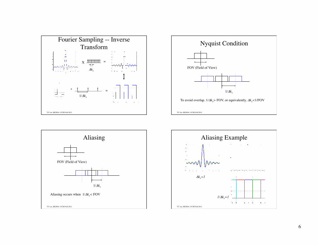
Fourier Sampling -- Inverse Transform
Χ =
*
1/Δkx
Δkx
=
TT. Liu, BE280A, UCSD Fall 2012
Nyquist Condition
FOV (Field of View)
1/Δkx
To avoid overlap, 1/Δkx> FOV, or equivalently, Δkx<1/FOV
TT. Liu, BE280A, UCSD Fall 2012
Aliasing
FOV (Field of View)
1/Δkx
Aliasing occurs when 1/Δkx< FOV
TT. Liu, BE280A, UCSD Fall 2012
Aliasing Example
Δkx=1
1/Δkx=1
7
TT. Liu, BE280A, UCSD Fall 2012
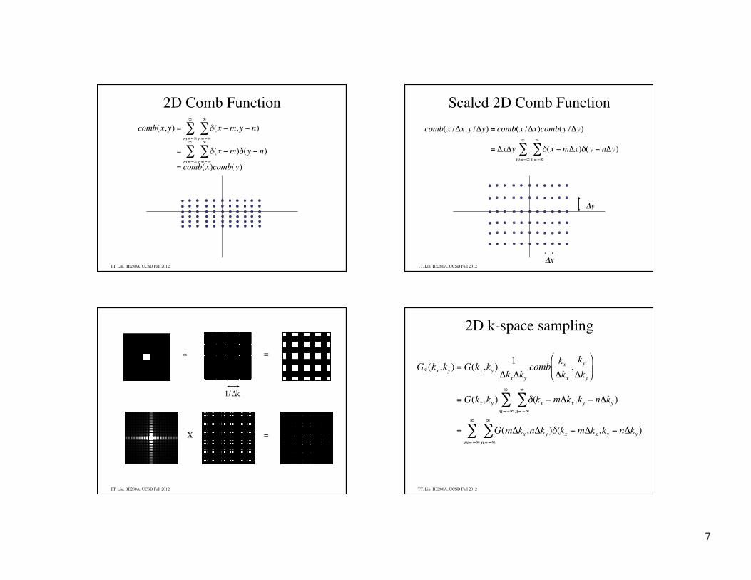
2D Comb Function
€
comb(x,y) = δ(x −m,y − n)n=−∞
∞
∑m=−∞
∞
∑
= δ(x −m)δ(y − n)n=−∞
∞
∑m=−∞
∞
∑= comb(x)comb(y)
TT. Liu, BE280A, UCSD Fall 2012
Scaled 2D Comb Function
€
comb(x /Δx,y /Δy) = comb(x /Δx)comb(y /Δy)
= ΔxΔy δ(x −mΔx)δ(y − nΔy)n=−∞
∞
∑m=−∞
∞
∑
Δx
Δy
TT. Liu, BE280A, UCSD Fall 2012
X =
* =
1/∆k
TT. Liu, BE280A, UCSD Fall 2012
2D k-space sampling
€
GS (kx,ky ) =G(kx,ky )1
ΔkxΔkycomb kx
Δkx,kyΔky
#
$ % %
&
' ( (
=G(kx,ky ) δ(n=−∞
∞
∑ kx −mΔkx,ky − nΔky )m=−∞
∞
∑
= G(mΔkx,nΔky )δ(n=−∞
∞
∑ kx −mΔkx,ky − nΔky )m=−∞
∞
∑
8
TT. Liu, BE280A, UCSD Fall 2012
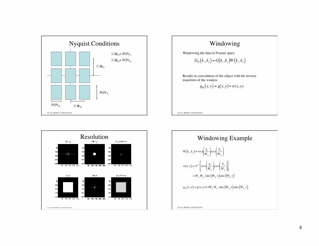
Nyquist Conditions
FOVX
FOVY
1/∆kX
1/∆kY
1/∆kY> FOVY
1/∆kX> FOVX
TT. Liu, BE280A, UCSD Fall 2012
Windowing
€
GW kx,ky( ) =G kx,ky( )W kx,ky( )
€
gW x,y( ) = g x,y( )∗w(x,y)
Windowing the data in Fourier space
Results in convolution of the object with the inverse transform of the window
TT. Liu, BE280A, UCSD Fall 2012
Resolution
TT. Liu, BE280A, UCSD Fall 2012
Windowing Example
€
W kx,ky( ) = rect kxWkx
"
# $ $
%
& ' ' rect
kyWky
"
# $ $
%
& ' '
€
w x,y( ) = F −1 rect kxWkx
#
$ % %
&
' ( ( rect
kyWky
#
$ % %
&
' ( (
)
* + +
,
- . .
=WkxWky
sinc Wkxx( )sinc Wky
y( )
€
gW x,y( ) = g(x,y)∗∗WkxWky
sinc Wkxx( )sinc Wky
y( )
9
TT. Liu, BE280A, UCSD Fall 2012
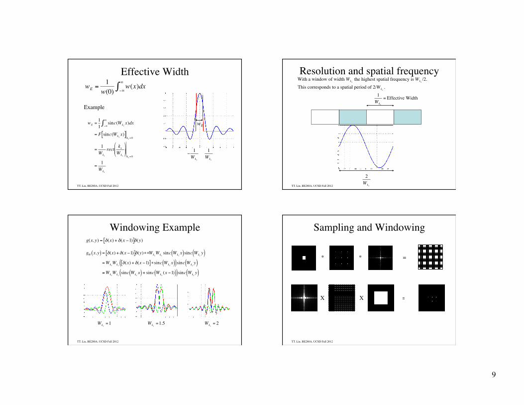
Effective Width
€
wE =1
w(0)w(x)dx
−∞
∞
∫
wE
€
wE =11
sinc(Wkxx)dx
−∞
∞
∫
= F sinc(Wkxx)[ ]
kx = 0
=1Wkx
rect kxWkx
%
& ' '
(
) * * kx = 0
=1Wkx
Example
€
1Wkx
€
−1Wkx
TT. Liu, BE280A, UCSD Fall 2012
Resolution and spatial frequency
€
2Wkx
€
With a window of width Wkx the highest spatial frequency is Wkx
/2.This corresponds to a spatial period of 2/Wkx
.
€
1Wkx
= Effective Width
TT. Liu, BE280A, UCSD Fall 2012
Windowing Example
€
g(x,y) = δ(x) + δ(x −1)[ ]δ(y)
€
gW x,y( ) = δ(x) + δ(x −1)[ ]δ(y)∗∗WkxWky
sinc Wkxx( )sinc Wky
y( )=Wkx
Wkyδ(x) + δ(x −1)[ ]∗ sinc Wkx
x( )( )sinc Wkyy( )
=WkxWky
sinc Wkxx( ) + sinc Wkx
(x −1)( )( )sinc Wkyy( )
€
Wkx=1
€
Wkx= 2
€
Wkx=1.5
TT. Liu, BE280A, UCSD Fall 2012
Sampling and Windowing
X =
* =
X
* =
10
TT. Liu, BE280A, UCSD Fall 2012
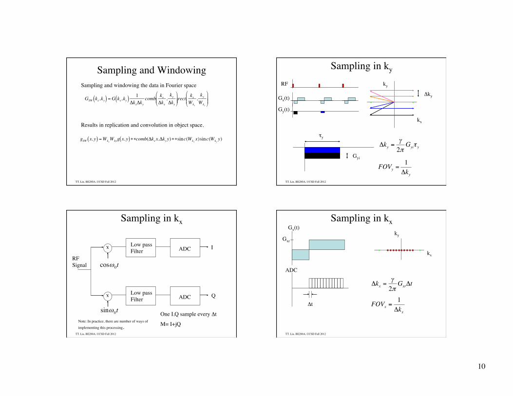
Sampling and Windowing
€
GSW kx,ky( ) =G kx,ky( ) 1ΔkxΔky
comb kxΔkx
,kyΔky
#
$ % %
&
' ( ( rect
kxWkx
,kyWky
#
$ % %
&
' ( (
€
gSW x,y( ) =WkxWkyg x,y( )∗∗comb(Δkxx,Δkyy)∗∗sinc(Wkx
x)sinc(Wkyy)
Sampling and windowing the data in Fourier space
Results in replication and convolution in object space.
TT. Liu, BE280A, UCSD Fall 2012
Sampling in ky
kx
ky
Gx(t)
Gy(t)
RF
Δky
τy
Gyi
€
Δky =γ2π
Gyiτ y
€
FOVy =1Δky
TT. Liu, BE280A, UCSD Fall 2012
Sampling in kx
x Low pass Filter ADC
x Low pass Filter ADC €
cosω0t
€
sinω0t
RF Signal
One I,Q sample every Δt
M= I+jQ
I
Q
Note: In practice, there are number of ways of implementing this processing.
TT. Liu, BE280A, UCSD Fall 2012
Sampling in kx
kx
ky
€
Δkx =γ2π
GxrΔt
€
FOVx =1Δkx
Gx(t)
t1
ADC
Gxr
Δt

11
TT. Liu, BE280A, UCSD Fall 2012
Resolution
€
δx =1Wkx
= 12kx,max
= 1γ
2πGxrτ x
€
Wkx€
Wky
Gx(t) Gxr
€
τ x
€
δy =1Wky
= 12ky,max
= 1γ
2π2Gypτ y
Gy(t)
τy €
Gyp
TT. Liu, BE280A, UCSD Fall 2012
Example
€
Goal :FOVx = FOVy = 25.6 cmδx = δy = 0.1 cm
€
Readout Gradient :
FOVx =1
γ2π
GxrΔt
Pick Δt = 32 µsec
Gxr =1
FOVxγ
2πΔt
=1
25.6cm( ) 42.57 ×10⁶T−1s−1( ) 32 ×10−6 s( )
= 2.8675 ×10⁻⁵ T/cm = .28675 G/cm
1 Gauss = 1×10⁻⁴ Tesla
t1
ADC
Gxr
Δt
TT. Liu, BE280A, UCSD Fall 2012
Example
€
Readout Gradient :
δx =1
γ2π
Gxrτ x
τ x =1
δxγ
2πGxr
=1
0.1cm( ) 4257 G−1s−1( ) 0.28675 G/cm( )
= 8.192 ms = NreadΔtwhere
Nread =FOVxδx
= 256
Gx(t)
Gxr
€
τ x
TT. Liu, BE280A, UCSD Fall 2012
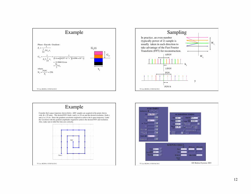
Example
€
Phase - Encode Gradient :
FOVy =1
γ2π
Gyiτ y
Pick τ y = 4.096 msec
Gyi =1
FOVyγ
2πτ y
=1
25.6cm( ) 42.57 ×10⁶T−1s−1( ) 4.096 ×10⁻³ s( )
= 2.2402 ×10⁻⁷ T/cm = .00224 G/cm
τy
Gyi
12
TT. Liu, BE280A, UCSD Fall 2012
Example
€
Phase - Encode Gradient :δy =
1γ
2π2Gypτ y
Gyp =1
δy 2 γ2π
τ y
=1
0.1cm( ) 4257 G−1s−1( ) 4.096 ×10⁻³ s( ) = 0.2868 G/cm
=Np
2Gyi
where
Np =FOVyδy
= 256
Gy(t)
τy €
Gyp
TT. Liu, BE280A, UCSD Fall 2012
Sampling
€
Wkx€
Wky
In practice, an even number (typically power of 2) sample is usually taken in each direction to take advantage of the Fast Fourier Transform (FFT) for reconstruction.
ky
y
FOV/4
1/FOV
4/FOV
FOV
TT. Liu, BE280A, UCSD Fall 2012
Example Consider the k-space trajectory shown below. ADC samples are acquired at the points shownwith
€
Δt = 10 µsec. The desired FOV (both x and y) is 10 cm and the desired resolution (both xand y) is 2.5 cm. Draw the gradient waveforms required to achieve the k-space trajectory. Labelthe waveform with the gradient amplitudes required to achieve the desired FOV and resolution.Also, make sure to label the time axis correctly.
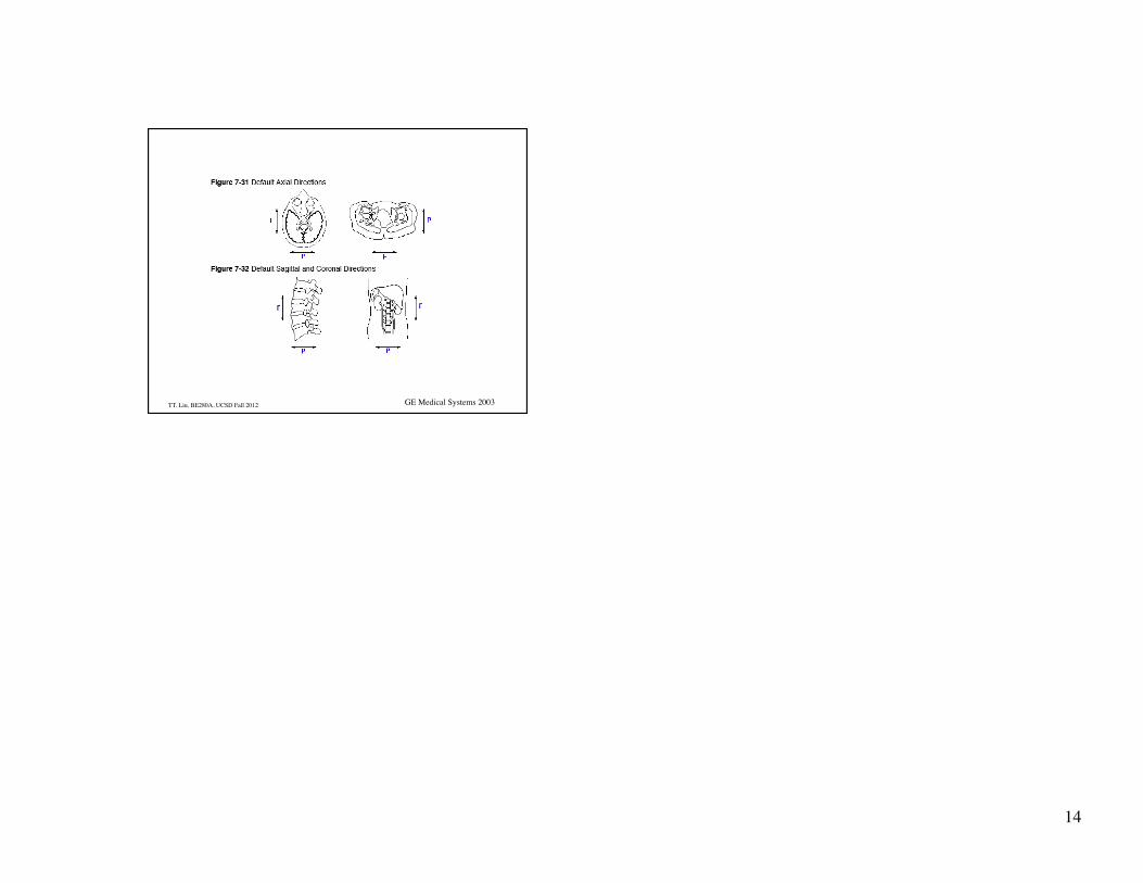
TT. Liu, BE280A, UCSD Fall 2012 GE Medical Systems 2003
13
TT. Liu, BE280A, UCSD Fall 2012
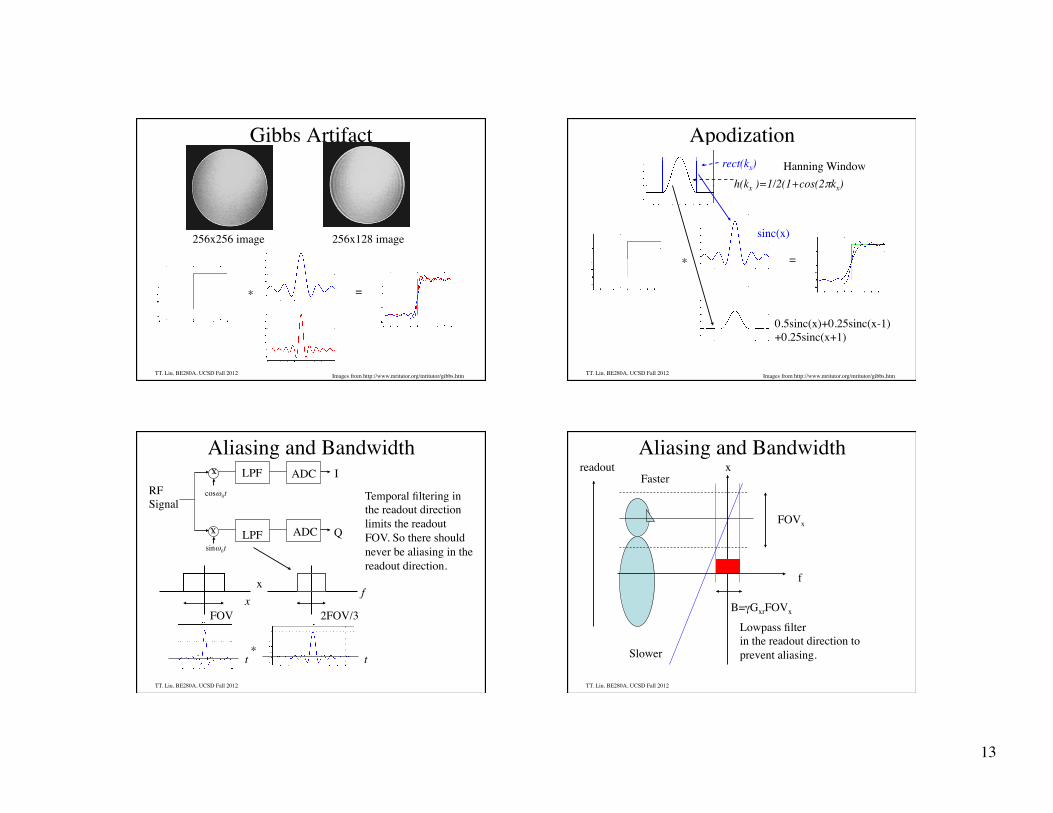
Gibbs Artifact
256x256 image 256x128 image
Images from http://www.mritutor.org/mritutor/gibbs.htm
* =
TT. Liu, BE280A, UCSD Fall 2012
Apodization
Images from http://www.mritutor.org/mritutor/gibbs.htm
* =
rect(kx)
h(kx )=1/2(1+cos(2πkx) Hanning Window
sinc(x)
0.5sinc(x)+0.25sinc(x-1) +0.25sinc(x+1)
TT. Liu, BE280A, UCSD Fall 2012
Aliasing and Bandwidth
x
LPF ADC
ADC €
cosω0t
€
sinω0t
RF Signal
I
Q LPF
x
*
x f
t
x
t
FOV 2FOV/3
Temporal filtering in the readout direction limits the readout FOV. So there should never be aliasing in the readout direction.
TT. Liu, BE280A, UCSD Fall 2012
Aliasing and Bandwidth
Slower
Faster x
f
Lowpass filter in the readout direction to prevent aliasing.
readout
FOVx
B=γGxrFOVx
14
TT. Liu, BE280A, UCSD Fall 2012 GE Medical Systems 2003
Related Documents