HAL Id: hal-03363459 https://hal.archives-ouvertes.fr/hal-03363459 Submitted on 4 Oct 2021 HAL is a multi-disciplinary open access archive for the deposit and dissemination of sci- entific research documents, whether they are pub- lished or not. The documents may come from teaching and research institutions in France or abroad, or from public or private research centers. L’archive ouverte pluridisciplinaire HAL, est destinée au dépôt et à la diffusion de documents scientifiques de niveau recherche, publiés ou non, émanant des établissements d’enseignement et de recherche français ou étrangers, des laboratoires publics ou privés. Modified Constitutive Relation Error for field identification : theoretical and experimental assessments on fiber orientation identification in a composite material Renaud Ferrier, Aldo Cocchi, Christian Hochard To cite this version: Renaud Ferrier, Aldo Cocchi, Christian Hochard. Modified Constitutive Relation Error for field identification : theoretical and experimental assessments on fiber orientation identification in a composite material. International Journal for Numerical Methods in Engineering, Wiley, 2021, 10.1002/nme.6842. hal-03363459

Welcome message from author
This document is posted to help you gain knowledge. Please leave a comment to let me know what you think about it! Share it to your friends and learn new things together.
Transcript
HAL Id: hal-03363459https://hal.archives-ouvertes.fr/hal-03363459
Submitted on 4 Oct 2021
HAL is a multi-disciplinary open accessarchive for the deposit and dissemination of sci-entific research documents, whether they are pub-lished or not. The documents may come fromteaching and research institutions in France orabroad, or from public or private research centers.
L’archive ouverte pluridisciplinaire HAL, estdestinée au dépôt et à la diffusion de documentsscientifiques de niveau recherche, publiés ou non,émanant des établissements d’enseignement et derecherche français ou étrangers, des laboratoirespublics ou privés.
Modified Constitutive Relation Error for fieldidentification : theoretical and experimental assessments
on fiber orientation identification in a compositematerial
Renaud Ferrier, Aldo Cocchi, Christian Hochard
To cite this version:Renaud Ferrier, Aldo Cocchi, Christian Hochard. Modified Constitutive Relation Error for fieldidentification : theoretical and experimental assessments on fiber orientation identification in acomposite material. International Journal for Numerical Methods in Engineering, Wiley, 2021,�10.1002/nme.6842�. �hal-03363459�
Received: Added at production Revised: Added at production Accepted: Added at production
DOI: xxx/xxxx
RESEARCH ARTICLE
Modified Constitutive Relation Error for field identification :
theoretical and experimental assessments on fiber orientation
identification in a composite material
Renaud Ferrier* | Aldo Cocchi | Christian Hochard
1LMA, Aix-Marseille Université, Marseille,France
Correspondence*Renaud Ferrier. Email:[email protected]
Present Address4 impasse Nikola Tesla, 13013 Marseille,France
Summary
This study addresses the application of the modified Constitutive Relation Error tofield identification problems in the framework of elastostatics. We show how rele-vant is the addition of a gradient-penalizing regularization term (in norm L1 or L2),and emphasize the role played by unreliable boundary conditions. This leads to theproposition of a method using two parameters, for which automatic determinationis addressed. All theoretical assessments are illustrated on experimental data. Thetest-problem consists in the identification of the heterogeneous fiber-orientation ina woven fabric composite from a unique quasi-static tensile test with digital imagecorrelation.
KEYWORDS:field identification, constitutive relation error, regularization, boundary conditions
1 INTRODUCTION
Inverse field identification problems arise in many practical applications. For example in defect imaging, when we want to
identify a zone where a given material parameter is far from the expected value. Another example is that of a sample in which
the medium is heterogeneous because of the production process. In such a case, the knowledge of the material parameter field
may be very approximate, which makes further numerical computations unreliable.
In this context, we suppose that an experimental test has been carried out to map a parameter’s distribution by using partial
measurements of the sample’s response to a known excitation. In the experimental example of this article, the parameter to
identify is the orientation of fibers in a composite, the excitation is a quasi-static tension load and the measurement is obtained by
2 FERRIER ET AL
digital image correlation (DIC). This particular problem has been chosen because it is possible to obtain a reference orientation
field by simple observation, and thus to evaluate the performance of the identification process.
The most straightforward identification method consists in finding the field of parameters that minimizes the difference
between the experimental measurement and the same measurement simulated with a direct computation. This method is called
PDE-constrained least-square minimization, and can also be found under the name Finite Element Method Update (FEMU).
It is presented, among others, in1. In this study, we will use the modified Constitutive Relation Error (m-CRE), that has many
similarities with least-square minimization.
The m-CRE method (also sometimes referred as MECE for Modified Error in Constitutive Equation) has been originally
applied to identification under free vibration in2. Since then, it has been successfully applied on many different inverse problems,
among which we can mention the identification of material parameters in the framework of transient dynamics3,4, identification
in static elasticity5 and defect identification in composites under compressive load, leading to buckling6.
The iterative identification methods studied in this paper require to solve several forward problems. As a consequence, the
quality of the identification is expected to depend on the validity of the hypotheses made on these forward problems, and in
particular, the Boundary Conditions (BC). In5 and7, the authors show how to use respectively m-CRE and least-square methods
without having to feed the model with unreliable BC. They show that the quality of the identification is significantly better by
this means.
Given that parameter identification problems are very often prone to instability, the use of regularization methods is an essen-
tial tool to obtain a solution that makes physical meaning. More precisely, the cost-function tends to be unable to discriminate
different candidate-solutions, and the regularization consists in choosing the right solution among them. Of course, the meaning
of right is a complex issue that must be defined for each particular application. Such regularization methods include for example
the Truncated (Generalized) SVD8, or the Tikhonov method, of which one of the first occurrences can be found in9. Another
approach, often used in the context of Constitutive Relation Error is to limit the number of iterations of the iterative algorithm.
This is used for example in6.
In a first part, we present the test-problem, namely the identification of an heterogeneous field of fibers orientations in a
composite, as well as the experimental setting. The second part is dedicated to the least-square minimization method and the
m-CRE method. We recall how it is possible to ignore unreliable boundary conditions with the m-CRE method. The third
part presents the minimization strategy, as well as the regularization procedure. Two different gradient-penalizing terms are
presented, along with their theoretical pros and cons. The last part is dedicated to the numerical evaluation of the different
proposed regularization strategies, as well as the different variants of the method.

FERRIER ET AL 3
2 PRESENTATION OF THE APPLICATION PROBLEM
Let us consider a part manufactured with a woven fabric-reinforced composite. During the forming process, before the polymer-
ization, the part can be subjected to forming stresses which change the warp and weft orientation. This leads to an heterogeneous
field of fibers orientation, that will be fixed during polymerization. This problem is for example studied in10. In11, the authors
show how to carry on a numerical structure computation from the knowledge of this field of orientations.
In Section 2.3, we show that this field can be determined through a simple observation of the sample. The resulting field will
be referred to as the reference orientation, and it will be used to evaluate the accuracy of the inverse procedure that consists in
identifying these angles from the knowledge of the displacement field on the sample during a tensile test that is carried out after
the polymerization.
2.1 Obtention of the test specimen
In our case, we consider a rectangular coupon manufactured with a twill woven carbon/epoxy composite and a [+45]S layup.
Before the polymerization, white lines parallel to the warp and weft directions are drawn on the surface of the sample. This
provides a referencemeasurement of the fiber orientation. Afterwards, the coupon is stretched in the longitudinal (0 deg) direction
and takes the deformed shape observed on Figure 1a.
(a) Deformed specimen (b) Undeformed (left) and deformed (right) woven fabriccomposite
FIGURE 1 Tensile stress specimen and representation of the material deformation
Once the specimen has been deformed, it is polymerized. The result is a planar test specimen whose fiber orientation is
heterogeneous.
4 FERRIER ET AL
2.2 From specimen realization to inverse solution
Once the heterogeneous test specimen has been obtained, a black and white speckle is painted on one of its faces and a tensile
test until failure is performed. During the test, images of the specimen are recorded. These images are processed by the software
GOM ARAMIS V512 in order to obtain a discretized displacement field at each time step corresponding to a picture.
0 0.2 0.4 0.6 0.8 1
0
500
1000
1500
2000
FmP
U (mm)
F(N
)
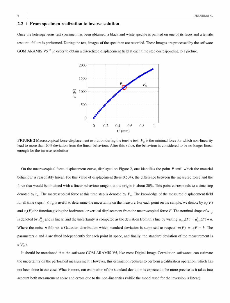
FIGURE 2Macroscopical force-displacement evolution during the tensile test. Fm is the minimal force for which non-linearitylead to more than 20% deviation from the linear behaviour. After this value, the behaviour is considered to be no longer linearenough for the inverse resolution
On the macroscopical force-displacement curve, displayed on Figure 2, one identifies the point P until which the material
behaviour is reasonably linear. For this value of displacement (here 0.504), the difference between the measured force and the
force that would be obtained with a linear behaviour tangent at the origin is about 20%. This point corresponds to a time step
denoted by tm. The macroscopical force at this time step is denoted by Fm. The knowledge of the measured displacement field
for all time steps ti ⩽ tm is useful to determine the uncertainty on the measure. For each point on the sample, we denote by ux(F )
and uy(F ) the function giving the horizontal or vertical displacement from the macroscopical force F . The nominal shape of ux,y
is denoted by u0x,y and is linear, and the uncertainty is computed as the deviation from this line by writing: ux,y(F ) = u0x,y(F )+n.
Where the noise n follows a Gaussian distribution which standard deviation is supposed to respect: �(F ) = aF + b. The
parameters a and b are fitted independently for each point in space, and finally, the standard deviation of the measurement is
�(Fm).
It should be mentioned that the software GOM ARAMIS V5, like most Digital Image Correlation softwares, can estimate
the uncertainty on the performed measurement. However, this estimation requires to perform a calibration operation, which has
not been done in our case. What is more, our estimation of the standard deviation is expected to be more precise as it takes into
account both measurement noise and errors due to the non-linearities (while the model used for the inversion is linear).
FERRIER ET AL 5
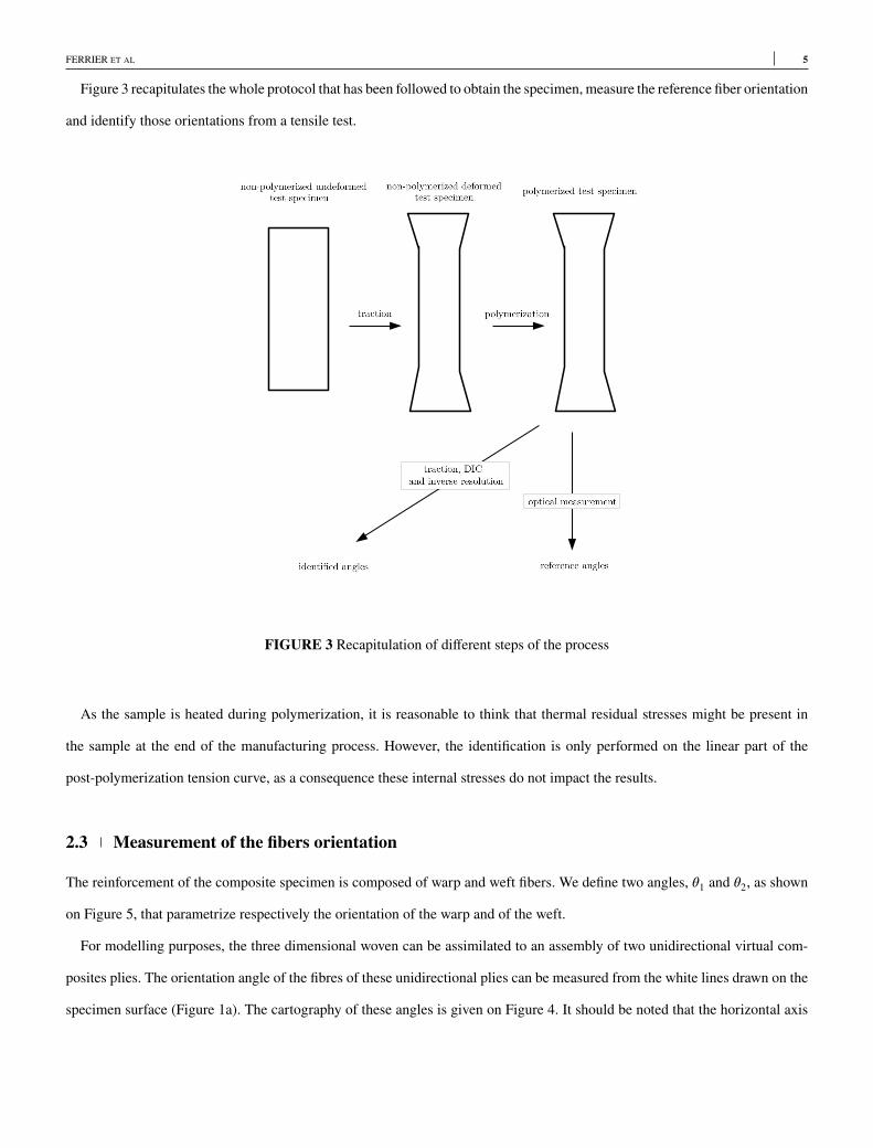
Figure 3 recapitulates the whole protocol that has been followed to obtain the specimen, measure the reference fiber orientation
and identify those orientations from a tensile test.
FIGURE 3 Recapitulation of different steps of the process
As the sample is heated during polymerization, it is reasonable to think that thermal residual stresses might be present in
the sample at the end of the manufacturing process. However, the identification is only performed on the linear part of the
post-polymerization tension curve, as a consequence these internal stresses do not impact the results.
2.3 Measurement of the fibers orientation
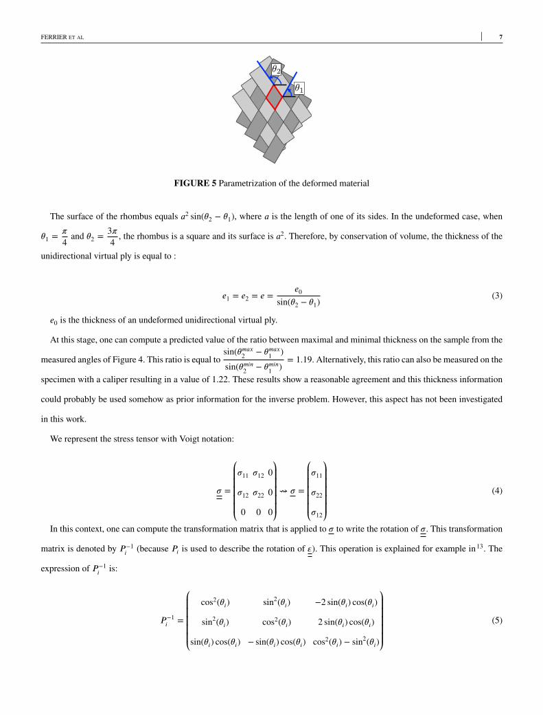
The reinforcement of the composite specimen is composed of warp and weft fibers. We define two angles, �1 and �2, as shown
on Figure 5, that parametrize respectively the orientation of the warp and of the weft.
For modelling purposes, the three dimensional woven can be assimilated to an assembly of two unidirectional virtual com-
posites plies. The orientation angle of the fibres of these unidirectional plies can be measured from the white lines drawn on the
specimen surface (Figure 1a). The cartography of these angles is given on Figure 4. It should be noted that the horizontal axis

6 FERRIER ET AL
on Figure 4 is mirrored respect to the one on Figure 1a because the sample has been reverted in the machine before proceeding
with the tensile test in order to present to the camera the side covered with a speckle.
FIGURE 4Measured angles
This map has a coarse spatial resolution, but it will however be used as a reference data to evaluate the accuracy of the inverse
computation.
2.4 Properties of the material as a function of the orientations
We determine the Hooke’s tensor of the homogenized bidimensional material in function of the two angles. LetHtot denote the
Hooke’s tensor in the specimen’s coordinate system.H1 andH2 are respectively the warp’s and the weft’s Hooke’s tensors.
Htot = H1 +H2 (1)
With :
Hi = eiP −1i H0P−Ti (2)
Where ei,H0 and P −1i are defined below.
ei is the thickness of the unidirectional virtual ply, that depends on �1 and �2. Let us consider the red polygon of Figure 5. If
we make the approximation that the fields �1 and �2 are homogeneous inside this polygon, its shape is a rhombus. Let us make
the hypothesis that the contact between warp and weft ensures that the fibers can not translate on the edges of this rhombus, but
only rotate. Therefore, the volume of material inside the rhombus is the same for all values of �1 and �2. Moreover, this volume
is equal to the surface of the rhombus multiplied by the thickness.
FERRIER ET AL 7
FIGURE 5 Parametrization of the deformed material
The surface of the rhombus equals a2 sin(�2 − �1), where a is the length of one of its sides. In the undeformed case, when
�1 =�4and �2 =
3�4, the rhombus is a square and its surface is a2. Therefore, by conservation of volume, the thickness of the
unidirectional virtual ply is equal to :
e1 = e2 = e =e0
sin(�2 − �1)(3)
e0 is the thickness of an undeformed unidirectional virtual ply.
At this stage, one can compute a predicted value of the ratio between maximal and minimal thickness on the sample from the
measured angles of Figure 4. This ratio is equal tosin(�max2 − �max1 )
sin(�min2 − �min1 )= 1.19. Alternatively, this ratio can also be measured on the
specimen with a caliper resulting in a value of 1.22. These results show a reasonable agreement and this thickness information
could probably be used somehow as prior information for the inverse problem. However, this aspect has not been investigated
in this work.
We represent the stress tensor with Voigt notation:
� =
⎛
⎜
⎜
⎜
⎜
⎜
⎝
�11 �12 0
�12 �22 0
0 0 0
⎞
⎟
⎟
⎟
⎟
⎟
⎠
⇝ � =
⎛
⎜
⎜
⎜
⎜
⎜
⎝
�11
�22
�12
⎞
⎟
⎟
⎟
⎟
⎟
⎠
(4)
In this context, one can compute the transformation matrix that is applied to � to write the rotation of �. This transformation
matrix is denoted by P −1i (because Pi is used to describe the rotation of "). This operation is explained for example in13. The
expression of P −1i is:
P −1i =
⎛
⎜
⎜
⎜
⎜
⎜
⎝
cos2(�i) sin2(�i) −2 sin(�i) cos(�i)
sin2(�i) cos2(�i) 2 sin(�i) cos(�i)
sin(�i) cos(�i) − sin(�i) cos(�i) cos2(�i) − sin2(�i)
⎞
⎟
⎟
⎟
⎟
⎟
⎠
(5)
8 FERRIER ET AL
One computes the derivatives :
)Hi
)�i=)ei)�i
P −1i H0P−Ti + ei
)P −1i)�i
H0P−Ti + eiP −1i H0
[
)P −1i)�i
]T
)e)�2
= − )e)�1
=cos(�2 − �1)sin2(�2 − �1)
)P −1i)�i
=
⎛
⎜
⎜
⎜
⎜
⎜
⎝
−2 cos(�i) sin(�i) 2 cos(�i) sin(�i) −2 cos2(�i) + 2 sin2(�i)
2 cos(�i) sin(�i) −2 cos(�i) sin(�i) 2 cos2(�i) − 2 sin2(�i)
cos2(�i) − sin2(�i) − cos2(�i) + sin
2(�i) −4 cos(�i) sin(�i)
⎞
⎟
⎟
⎟
⎟
⎟
⎠
(6)
It is worth noting that Htot is � periodic with respect to �1 and �2. As a consequence, the angles are not sought in ℝ, but in
[0, �]. This has no consequence provided, during the execution of the algorithm, the values taken by �i stay far form 0 and �.
One important point for the reliability of the identification is that the knowledge of the material parameter must itself be
reliable. This is of course not the case. One could propose to identify these parameters during a prior test on a part for which
the fiber orientation is known and homogeneous. In the present case, we prefer to add the 4 material parameters, supposed to
be uniform, to the unknowns. In order not to spoil the conditioning of the Hessian, the unknowns that are added in practice are
normalized by the initial values of the material parameters.
The Hooke’s tensorH0 and its derivatives with respect to the material parameters are computed:
H0 = S−10 =
⎛
⎜
⎜
⎜
⎜
⎜
⎜
⎝
1E1
−�12E1
0
−�12E1
1E2
0
0 0 1G12
⎞
⎟
⎟
⎟
⎟
⎟
⎟
⎠
−1
=
⎛
⎜
⎜
⎜
⎜
⎜
⎜
⎝
E21
E1 − �212E2
�12E1E2E1 − �212E2
0
�12E1E2E1 − �212E2
E1E2E1 − �212E2
0
0 0 G12
⎞
⎟
⎟
⎟
⎟
⎟
⎟
⎠
(7)
FERRIER ET AL 9
⎧
⎪
⎪
⎪
⎪
⎪
⎪
⎪
⎪
⎪
⎪
⎪
⎪
⎪
⎪
⎪
⎪
⎨
⎪
⎪
⎪
⎪
⎪
⎪
⎪
⎪
⎪
⎪
⎪
⎪
⎪
⎪
⎪
⎪
⎩
)H0
)E1= 1(E1 − �212E2)
2
⎛
⎜
⎜
⎜
⎜
⎜
⎜
⎝
E21 − 2�
212E1E2 −�3E2
2 0
−�312E22 −�212E
22 0
0 0 0
⎞
⎟
⎟
⎟
⎟
⎟
⎟
⎠
)H0
)E2= 1(E1 − �212E2)
2
⎛
⎜
⎜
⎜
⎜
⎜
⎜
⎝
E21�212 �12E2
1 0
�12E21 E2
1 0
0 0 0
⎞
⎟
⎟
⎟
⎟
⎟
⎟
⎠
)H0
)�12= 1(E1 − �212E2)
2
⎛
⎜
⎜
⎜
⎜
⎜
⎜
⎝
2E21E2�12 E2
1E2 + �212E1E
22 0
E21E2 + �
212E1E
22 2�12E1E2
2 0
0 0 0
⎞
⎟
⎟
⎟
⎟
⎟
⎟
⎠
)H0
)G12=
⎛
⎜
⎜
⎜
⎜
⎜
⎜
⎝
0 0 0
0 0 0
0 0 1
⎞
⎟
⎟
⎟
⎟
⎟
⎟
⎠
(8)
Practical tests show that the sensibility of the m-CRE cost function with respect to the parameters E2 and �12 is too low to
ensure a reliable identification. As a consequence, only E1 and G12 are identified.
The initial values taken for the material parameters are reported in (9).
⎧
⎪
⎪
⎪
⎪
⎨
⎪
⎪
⎪
⎪
⎩
E1 = 150 GPa
E2 = 10 GPa
�12 = 0.3
G12 = 3.8 GPa
(9)
3 FIELD IDENTIFICATION METHODS
The problem of interest is the identification of two (discretized) fields of parameters from displacement measurements. This
results in numerous unknowns, that can be gathered in a vectorial unknown, denoted by �. In the framework of linear elasto-
statics, the discretized direct problem consists in computing the displacement field on a discretized domain Ωℎ from the
10 FERRIER ET AL
knowledge of boundary conditions andmaterial parameters �. The problem is discretizedwith the Finite ElementMethod (FEM),
and � only influences the stiffness matrix, K(�). The direct problem can then be written under the following form:
u = argminx
Cx=�
12xT K(�)x − xT f (10)
u is the unknown displacement field on Ωℎ, Cx = � is a set of linear constraints that impose, among others, the discretized
Dirichlet Boundary Conditions (BC). One supposes that C has full row rank, which means that all constraints in Cx = � are
linearly independent. As a consequence, CCT is an invertible matrix.
The methods will be presented formally in the case when the constraints are satisfied by substitution, but they are of course
applicable with any constrained minimization method. One can show that Problem (10) is equivalent to Problem (11):
u = argminx
12xTK(�)x − xTf
K(�) = (d − CT (CCT )−1C)K(�)(d − CT (CCT )−1C) +KCT (CCT )−1C
f = (d − CT (CCT )−1C)(
f − K(�)CT (CCT )−1�)
+KCT (CCT )−1�
(11)
d is the identity matrix of the same size as K(�), and K is a scalar parameter, determined as an estimation of the spectral
radius of K(�). It prevents the resulting system from being ill-conditioned in the case when K(�) involves large moduli. In
practice, it is often not necessary to take this parameter different to 1.
Problem (11) reduces to the linear problem (12). This approach has the notational advantage that the solution of this problem
is exactly u, and not a restriction of it, nor a vector containing u and Lagrange multipliers.
K(�)u = f (12)
The inverse problem consists in computing � from the knowledge of a measured displacement, denoted by um. This measure-
ment was done on a particular grid, driven by the measurement method, which has no reason to coincide with the FE mesh. For
that reason, one introducesΠ, the observation operator such thatΠu is defined on the same grid as um. This observation operator
introduces an interpolation error that will be neglected in this work.
What is more, the question of the discretization of � is crucial for the well-posedness of the mathematical problem because
the more unknowns there are, the less stable the solution is. For the sake of simplicity, in this study, it has been decided to use
the FE mesh to discretize �. This results in the inverse problem being very unstable and most likely having no unique solution.
To solve this, and in order to make the solution mesh-independent, we introduce a regularizing (semi-) norm, denoted byN(�),
that is used to stabilize the solution. The weight of this term is tuned by a regularization parameter �.
FERRIER ET AL 11
3.1 Least-square minimization
One writes the following minimization problem, where the FE-discretized PDE K(�)u = f is added as a constraint:
min�,u
K(�)u=f
'(�, u)
'(�, u) = 12(
Πu − um)T (Πu − um
)
+ �N(�)
(13)
The problem (13) is equivalent to the search of the saddle point of the following Lagrangian:
�(�, u, �) = 12(
Πu − um)T (Πu − um
)
+ �N(�) + �T (K(�)u − f ) (14)
One can express the gradients of �:
⎧
⎪
⎪
⎪
⎨
⎪
⎪
⎪
⎩
∇u� = ΠT (Πu − um) +K(�)�
∇�� = K(�)u − f
∇�� = �∇N(�) + �T∇K(�)u
(15)
For solving (13), we use the BFGS method, as detailed in Section 4.1. In the present case, the BFGS method requires to find u
and � that make respectively ∇�� and ∇u� vanish. Therefore we solve the following direct and adjoint problems at each BFGS
iteration:
⎧
⎪
⎪
⎨
⎪
⎪
⎩
K(�)u = f
K(�)� = ΠT (um − Πu)(16)
3.2 Modified Constitutive Relation Error
In this section, we present a variant of the method of modified Constitutive Relation Error, in the case where there are available
and reliable Boundary Conditions on the entire boundary of the studied domain. This variant is called MCRE-I in5.
Let us introduce two displacement fields, that are defined on the FE mesh. v respects the global equilibrium, which means that
it is the unique solution to the direct problemK(�)v = f . AsK(�) is built as described in Equation (11), Cv = � is ensured. u is
supposed to be equal to the measured displacement, which meansΠu = um, but the modified CRE method relaxes this condition
by adding term penalizing the norm of Πu − um.
We choose to impose that u respects the Dirichlet BCs of the direct problem, ie. Cu = �. This assumption makes sure that u
and v are in the same space.
12 FERRIER ET AL
The minimization problem is the following:
min�,u,v
Cu=�,K(�)v=f
12(u − v)T K(�)(u − v) + r
2(
Πu − um)T (Πu − um
)
+ �rN(�) (17)
We remark that C(u − v) = 0, and given the expression of K(�) in Equation (11), we have
( u − v )T K(�) ( u − v ) = ( u − v )T K(�) ( u − v ), which allows to replace this term in (17), in order to obtain the
following minimization problem, that does not use K(�) anymore.
min�,u,v
Cu=�,K(�)v=f
12(u − v)TK(�)(u − v) + r
2(
Πu − um)T (Πu − um
)
+ �rN(�) (18)
In this method, two parameters have been introduced. The weighting parameter r tunes the importance given to the measure-
ments, and the regularization parameter� penalizes the fields � that have a high normN(�). Most authors use r as a regularization
parameter, as in14, where this parameter is changed at each iteration. In this context, r can be determined with the L-curve or
Morozov methods, that are exposed in Section 5.4.2.
The termN(�), while being very classical for the PDE-constrained least-square minimization method, is usually not used in
m-CRE method. To the author’s knowledge, the only occurrence of such a term in literature is very recent, in15, where a damage
field is identified. One of the objectives of this study is to show the benefit of using this term for identifying smooth fields.
Note that the regularizing term is multiplied by the parameter r in order to be consistent with the cost-function used by the
least-square method. The proposed cost-function is then a sum of a term proportional to ' from (13) and the new Constitutive
Relation Error term.
As previously, one can introduce the following Lagrangian, which saddle-point gives the solution to the problem:
�(�, u, v, �) = 12(u − v)TK(�)(u − v) + r
2(
Πu − um)T (Πu − um
)
+ �rN(�) + �T (K(�)v − f ) (19)
The gradients are:
⎧
⎪
⎪
⎪
⎪
⎨
⎪
⎪
⎪
⎪
⎩
∇u� = K(�)u −K(�)v + rΠTΠu − rΠT um
∇v� = K(�)v −K(�)u +K(�)�
∇�� = K(�)v − f
∇�� =12(u − v)T∇K(�)(u − v) + �r∇N(�) + �T∇K(�)v
(20)
FERRIER ET AL 13
Similarly to what was done in Section 3.1, one determines u, v and � by writing ∇u� = 0, ∇v� = 0 and ∇�� = 0. This leads
to solve the following uncoupled problems:
⎧
⎪
⎪
⎪
⎨
⎪
⎪
⎪
⎩
K(�)v = f
(K(�) + rΠTΠ)u = f + rΠT um
� = u − v
(21)
Two linear problems have to be solved. The computational cost is the same as in the least-square method of Section 3.1 at
one condition: the observation operator Π has to be sparse.
One can finally notice that the least-square minimization method is a limit case of modified Constitutive Relation Error. Let
us suppose that r = o(�), where � is the ratio between the spectral radii of K and ΠTΠ. We also suppose that � = O(p),
where p is the ratio between the spectral radius of ΠTΠ and GTG (see Section 4.2). Schematically, this means that the termsr2(
Πu − um)T (Πu − um
)
+�rN(�) aremuch smaller than 12(u−v)TK(�)(u−v) in�. In that case, as shown in16, and as illustrated
numerically in Section 5.2.3, the solution of the m-CREmethods tends towards the one of the least-square minimization method.
3.3 m-CRE without boundary conditions on a part of the boundary
As the measurement um results from an experimental test, it is very likely that some of the BCs of this test are not well known.
More specifically, for the case of a static tensile test, the displacement in the vicinity of the machine’s jaws is unknown. As a
consequence, we no longer take those BCs into account in the computation of v. This variant is called MCRE-II in5.
For the purpose of our application, we suppose in this part that all Dirichlet boundary conditions are ignored, which means
that there is no condition of the type Cu = �, and K(�) = K(�).
The Degrees Of Freedom (DOF) subjected to unknown forces are denoted with a ∅ index while the other ones, for which an
equilibrium relation can be written, are denoted with a 1 index.
One introduces the following decompositions for K and f , and a prolongation by zero of �, denoted by �2:
K(�) =
⎛
⎜
⎜
⎜
⎝
K11(�) K1∅(�)
KT1∅(�) K∅∅(�)
⎞
⎟
⎟
⎟
⎠
=
⎛
⎜
⎜
⎜
⎝
K1(�)
K∅(�)
⎞
⎟
⎟
⎟
⎠
f =
⎛
⎜
⎜
⎜
⎝
f1
f∅
⎞
⎟
⎟
⎟
⎠
�2 =
⎛
⎜
⎜
⎜
⎝
�
�∅
⎞
⎟
⎟
⎟
⎠
(22)
where �∅ is a null vector which size is the number of degrees of freedom with unknown force.
The known part of the equilibrium is:
K1(�)v = f1 (23)
14 FERRIER ET AL
The cost-function is slightly different from (18):
min�,u,v
K1(�)v=f1
12(u − v)TK(�)(u − v) + r
2(
Πu − um)T (Πu − um
)
+ �rN(�) (24)
The Lagrangian is also slightly different from (19):
�(�, u, v, �) = 12(u − v)TK(�)(u − v) + r
2(
Πu − um)T (Πu − um
)
+ �rN(�) + �T(
K1(�)v − f)
(25)
And the gradients are:
⎧
⎪
⎪
⎪
⎪
⎨
⎪
⎪
⎪
⎪
⎩
∇u� = K(�)u −K(�)v + rΠTΠu − rΠT um
∇v� = K(�)v −K(�)u +KT1 (�)�
∇�� = K1(�)v − f1
∇�� =12(u − v)T∇K(�)(u − v) + �r∇N(�) + �T∇K1(�)u
(26)
Contrary to what happens in Section 3.2, one can not uncouple the three problems ∇u� = 0, ∇v� = 0 and ∇�� = 0.
∇�� = 0 implies K1(�)v = f1 and ∇v� = 0 gives:
K(�)(u − v) = KT1 (�)� (27)
That can be restricted to the degrees of freedom where the force is known:
K1(�)(u − v) = K11(�)� (28)
We replace K(�)(u − v) by KT1 (�)� in ∇u� = 0, which implies:
KT1 (�)� = rΠ
T (um − Πu) (29)
From equations (29) and (28), one can write the system to determine u and �:
⎛
⎜
⎜
⎜
⎝
rΠTΠ KT1 (�)
K1(�) −K11(�)
⎞
⎟
⎟
⎟
⎠
⎛
⎜
⎜
⎜
⎝
u
�
⎞
⎟
⎟
⎟
⎠
=
⎛
⎜
⎜
⎜
⎝
rΠT um
f1
⎞
⎟
⎟
⎟
⎠
(30)
The physical problem that is solved by the system (30) is similar to a prolongation problem, and consists in finding a field
from measurements inside the domain and a PDE that governs the field, but without BCs. If some boundaries of the meshed
domain, on which u is defined, are far from any measurement point, this problem is ill-conditioned and a regularizing approach
must be used (see5). In extreme cases, one could even propose to use methods dedicated to this type of problem, like the one
FERRIER ET AL 15
introduced in17. However, in the cases that are studied here, we assume that there are always measurements close enough to the
bounds of the domain to ensure that the problem (30) is well-conditioned and can be solved without any particular care.
From Equation (27), one gets K(�)(u − v) = K(�)�2. We remark that the term that actually appears in � and its gradient is
K(�)v, and the vector v can be determined without any consideration for the kernel of K(�) by a simple subtraction:
v = u − �2 (31)
From this equation, one can deduce:
⎧
⎪
⎪
⎨
⎪
⎪
⎩
(u − v)TK(�)(u − v) = �T2K(�)�2 = �TK11(�)�
(u − v)T∇K(�)(u − v) = �T2∇K(�)�2 = �T∇K11(�)�
(32)
These equations lead to more practical and less CPU-costly expressions of the cost-function and its gradient.
4 MINIMIZATION AND REGULARIZATION
The performance of an inversion method depends largely on the choice of the minimization method, as well as the regularizing
approach.
4.1 Minimization method
All methods presented in Section 3 consist in searching for a saddle-point of a function denoted by �(�, u, v, �). If we suppose
that the saddle-point is unique, one can denote it by the notation argstat (the argument of the stationarity problem).
The saddle-point is a minimum in the direction �. One can then introduce a function of �:
(�) = �(�, u(�), v(�), �(�))
Where{
u(�), v(�), �(�)}
= argstatu,v,�
�(�, u, v, �)(33)
We will minimize with the BFGS method. This consists in an iterative method that requires, at each iteration i, to evaluate
(�i) and its gradient ∇ (�i), which coincides with ∇��(�, u(�), v(�), �(�)), as shown in the following equation:
∇ = ∇�� +[
∇u�]T
⏟⏟⏟=0
∇� u +[
∇v�]T
⏟⏟⏟=0
∇� v +[
∇��]T
⏟⏟⏟=0
∇�� = ∇�� (34)
16 FERRIER ET AL
For the Hessian of , the BFGS method (see for example18) consists in approximating it by a matrix i, that is obtained
through an updating process that adds two new terms of rank 1 after each iteration.
yi = ∇ (�i) − ∇ (�i−1)
�i = �i − �i−1
i+1 = i +yiyTiyTi �i
−i�i�Ti i
�Ti i�i
(35)
0 is initialized as a real parameter � times the identity matrix . By this means, the first iteration of the method consists in
a steepest descent step. � has the dimension of an energy in our case where � is dimensionless, but the choice of its value is not
crucial as the step is tuned during the line-search procedure.
Newton’s method is applied on the gradient of , which results in each iterate to be written as follows:
�i+1 = �i −−1i ∇ (�i) (36)
When � is updated in (36), we don’t use the true Hessian, moreover, the cost-function can be arbitrarily far from a quadratic
function. For these reasons, nothing ensures that (�i+1) is actually lower than (�i). This is why the following line-search
procedure may be essential for the convergence of the algorithm.
The idea is to use the direction given by equation (36). One searches, along the ray [�i, �i+1), the point �i+1 that realizes the
minimum of . This can for example be done by dichotomy. in the present case, our algorithm is even simpler and consists
in dividing the step by 2 until (�i+1) < (�i). The advantage is that if �i+1 satisfies this condition (which often occurs), the
procedure does not require any more evaluation of .
Let us emphasize that is a full matrix. As a consequence, in the case where its size is big (one or a few values per Gauss
point of a FE mesh), the inversion of the linear system may be numerically costly.
The BFGSmethod can converge towards any kind of stationary point of . As a consequence, this procedure is a minimization
method only if the cost-function is convex. In practice, it is not possible to ensure this, and one simply supposes that is
locally convex in a given neighbourhood around its minimum, and that all iterates are in this neighbourhood. This is obviously
not always true, that is why the choice of the initialization is important. In this study, two different initialization strategies are
proposed in Section 4.2, that depend on the chosen regularizing term.
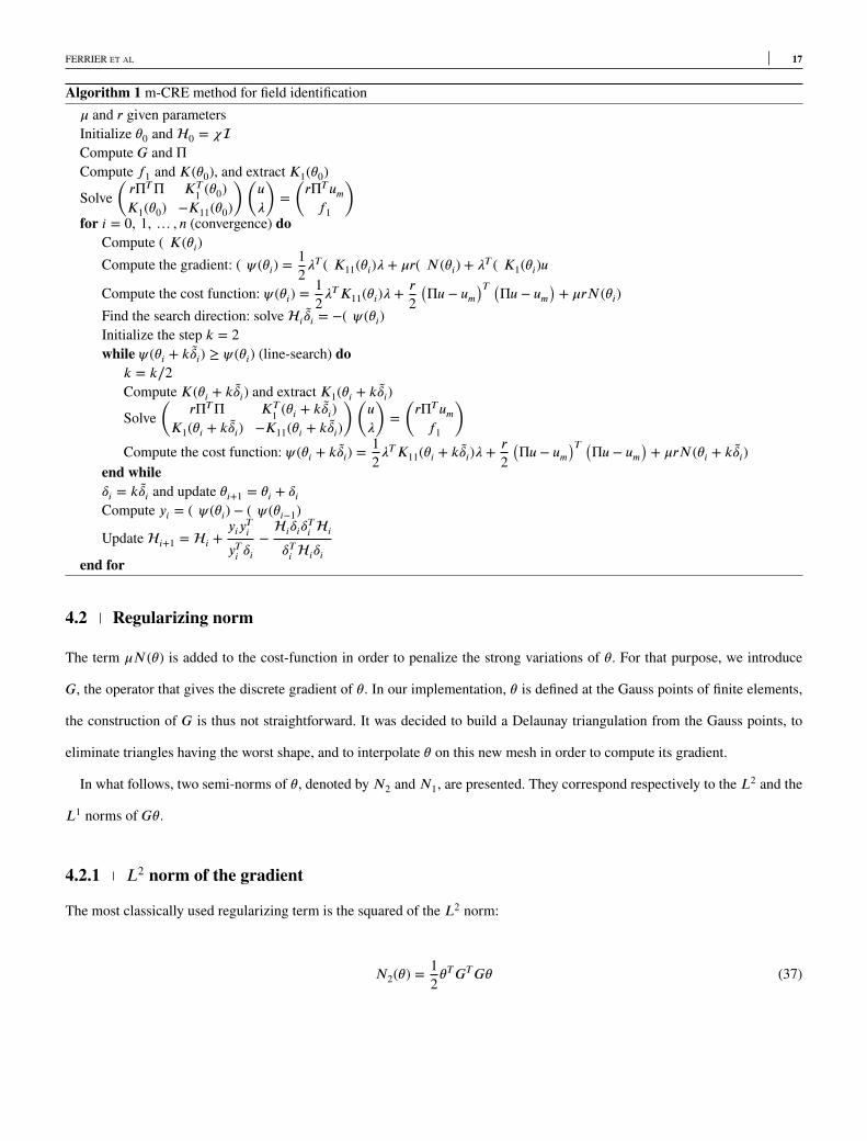
The m-CRE identification algorithm with the BFGS optimization method, and unreliable boundary conditions is summarized
on Algorithm 1.
FERRIER ET AL 17
Algorithm 1 m-CRE method for field identification� and r given parametersInitialize �0 and 0 = �Compute G and ΠCompute f1 and K(�0), and extract K1(�0)
Solve(
rΠTΠ KT1 (�0)
K1(�0) −K11(�0)
)(
u�
)
=(
rΠT umf1
)
for i = 0, 1, … , n (convergence) doCompute ∇K(�i)Compute the gradient: ∇ (�i) =
12�T∇K11(�i)� + �r∇N(�i) + �T∇K1(�i)u
Compute the cost function: (�i) =12�TK11(�i)� +
r2(
Πu − um)T (Πu − um
)
+ �rN(�i)Find the search direction: solve i�i = −∇ (�i)Initialize the step k = 2while (�i + k�i) ≥ (�i) (line-search) do
k = k∕2Compute K(�i + k�i) and extract K1(�i + k�i)
Solve(
rΠTΠ KT1 (�i + k�i)
K1(�i + k�i) −K11(�i + k�i)
)(
u�
)
=(
rΠT umf1
)
Compute the cost function: (�i + k�i) =12�TK11(�i + k�i)� +
r2(
Πu − um)T (Πu − um
)
+ �rN(�i + k�i)end while�i = k�i and update �i+1 = �i + �iCompute yi = ∇ (�i) − ∇ (�i−1)
Update i+1 = i +yiyTiyTi �i
−i�i�Ti i
�Ti i�iend for
4.2 Regularizing norm
The term �N(�) is added to the cost-function in order to penalize the strong variations of �. For that purpose, we introduce
G, the operator that gives the discrete gradient of �. In our implementation, � is defined at the Gauss points of finite elements,
the construction of G is thus not straightforward. It was decided to build a Delaunay triangulation from the Gauss points, to
eliminate triangles having the worst shape, and to interpolate � on this new mesh in order to compute its gradient.
In what follows, two semi-norms of �, denoted byN2 andN1, are presented. They correspond respectively to the L2 and the
L1 norms of G�.
4.2.1 L2 norm of the gradient
The most classically used regularizing term is the squared of the L2 norm:
N2(�) =12�TGTG� (37)
18 FERRIER ET AL
The computation of its gradient leads to:
∇�N2(�) = GTG� (38)
When this norm is used, the unknown parameter vector � can be initialized as a homogeneous field equal to (or rather not so
far from) the expected mean of the parameter distribution.
4.2.2 L1 norm of the gradient
In the context of image restoration19 or compressed sensing20, many authors have proposed to use regularization terms that are
based on theL1 norm. This norm, alongwith theL0 and otherLp, 0 < p < 1 norms, may be used to obtain a sparse representation
of a set of unknowns. The review paper21 presents mathematical investigations and algorithms used in this framework.
To understand the potential benefit of using the L1 norm of the gradient rather than the squared of its L2 norm, one can com-
pare, in the continuous unidirectional framework, the value of these two norms, denoted by ‖f‖p,ℝ, for the classical arctangent
smoothed step function:
k ∈ ℝ, f ∶ x ∈ ℝ → arctan(kx)
‖f‖22,ℝ =
∞
∫−∞
(
f ′(x))2 dx = k2 �
2and ‖f‖1,ℝ =
∞
∫−∞
|
|
f ′(x)||
dx = �(39)
When k is low, the function f is smooth, while when k tends towards∞, it is known to approach a step function. One notices
by the expressions of (39) that the L2 norm of the gradient unsurprisingly increases with k, while the L1 norm remains the
same. This last norm only takes into account the total amount of absolute variation of the studied function, and not the rate of
this variation. This is why it is often referred as the Total Variation term.
Penalizing the L2 norm favours smooth variations (lower k in our example) while penalizing the L1 norm preserves sharp
frontiers between quite homogeneous zones. It is very interesting if the parameter is suspected to obey to such a spatial
distribution.
In the discrete framework, if (G�)i is the i-th term of the vector G�, one has:
N1(�) =∑
i|(G�)i| (40)
This norm has the inconvenient to be non-smooth and non-differentiable. As a consequence, the resolution of the regular-
ized minimization problem requires to use dedicated methods, as proposed in19 or22. However, in our case, for simplicity, we
FERRIER ET AL 19
prefer to use the more common BFGS algorithm. For this purpose, we propose to use a well-known smooth and differentiable
approximation ofN1(�), which is calledN�1 (�) and defined on Equation (41).
N�1 (�) =
∑
i
√
((G�)i)2 + � (41)
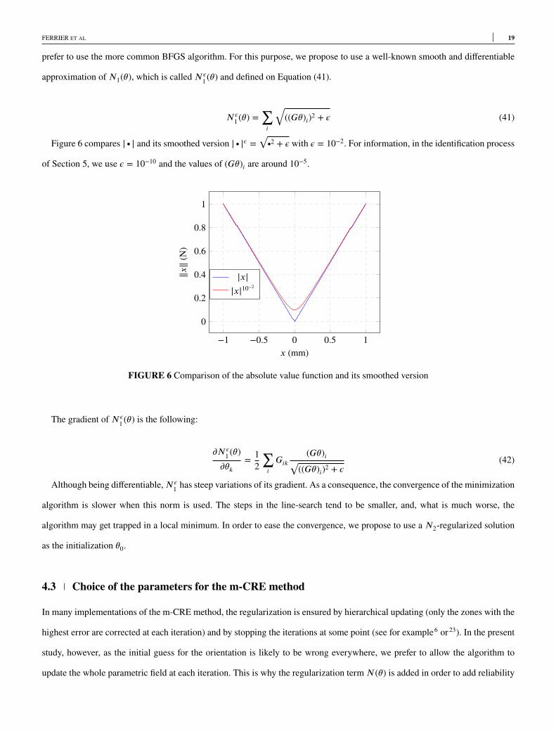
Figure 6 compares | ∙ | and its smoothed version | ∙ |� =√
∙2 + � with � = 10−2. For information, in the identification process
of Section 5, we use � = 10−10 and the values of (G�)i are around 10−5.
−1 −0.5 0 0.5 1
0
0.2
0.4
0.6
0.8
1
x (mm)
‖x‖
(N)
|x||x|10−2
FIGURE 6 Comparison of the absolute value function and its smoothed version
The gradient ofN�1 (�) is the following:
)N�1 (�))�k
= 12∑
iGik
(G�)i√
((G�)i)2 + �(42)
Although being differentiable,N�1 has steep variations of its gradient. As a consequence, the convergence of the minimization
algorithm is slower when this norm is used. The steps in the line-search tend to be smaller, and, what is much worse, the
algorithm may get trapped in a local minimum. In order to ease the convergence, we propose to use a N2-regularized solution
as the initialization �0.
4.3 Choice of the parameters for the m-CRE method
In many implementations of the m-CRE method, the regularization is ensured by hierarchical updating (only the zones with the
highest error are corrected at each iteration) and by stopping the iterations at some point (see for example6 or23). In the present
study, however, as the initial guess for the orientation is likely to be wrong everywhere, we prefer to allow the algorithm to
update the whole parametric field at each iteration. This is why the regularization termN(�) is added in order to add reliability
20 FERRIER ET AL
to the field identification method. The drawback is that one has to tune two parameters, � and r, instead of one. We then propose
a way to a-priori choose a value for r, while � will be determined thanks to a L-curve24,25.
We will use �, the ratio of spectral radii of K and ΠTΠ. In practice, the computation of spectral radii is numerically costly,
this is why in the numerical part, � will be replaced by �, which is the ratio of Frobenius norms.
In5, it appears that the main advantage of the m-CRE method is the ability to dispense with unreliable BCs. Numerical tests
done in Section 5.2 tend to confirm this. As a consequence, we can choose for the weighting parameter r any value that is small
compared to �. For example, r = 10−3�. The method then tends towards PDE-constrained optimization, with the advantage of
being able to ignore Dirichlet BCs. One can refer to Section 5.2.3, where the distance between the solution of m-CRE method
(with BCs) and PDE-constrained optimization is numerically studied.
Another way to explain the choice of r is by assuming that, as demonstrated in the context of time-harmonic elasticity in the
theorem 2 of16, the higher is r, the more the problem is regularized. In the context of the proposed method, the regularization is
rather performed by the termN(�), and the role of r is simply to provide a non-singular BC-free system. This is why any small
value can be chosen, provided it ensures a correct condition number for the coupled problem (30).
5 NUMERICAL RESULTS
5.1 Boundary Conditions of the direct computation
For the least-square minimization and standard m-CRE method of Sections 3.1 and 3.2, one needs to impose boundary condi-
tions to the direct computation. It has been chosen to apply null displacements to the lower boundary (as it is blocked by the
testing machine’s jaw), to impose zero Neumann BCs on the lateral boundaries, and an homogeneous displacement on the upper
boundary. The numerical value of the imposed vertical displacement is the mean of the measured displacement on this line,
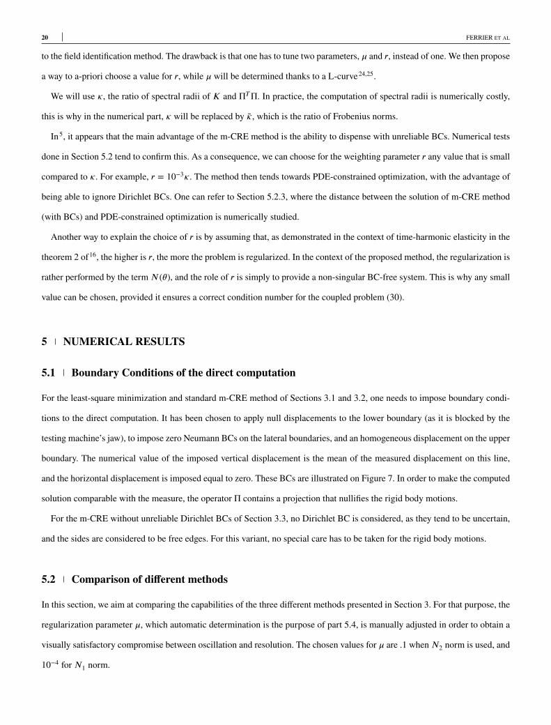
and the horizontal displacement is imposed equal to zero. These BCs are illustrated on Figure 7. In order to make the computed
solution comparable with the measure, the operator Π contains a projection that nullifies the rigid body motions.
For the m-CRE without unreliable Dirichlet BCs of Section 3.3, no Dirichlet BC is considered, as they tend to be uncertain,
and the sides are considered to be free edges. For this variant, no special care has to be taken for the rigid body motions.
5.2 Comparison of different methods
In this section, we aim at comparing the capabilities of the three different methods presented in Section 3. For that purpose, the
regularization parameter �, which automatic determination is the purpose of part 5.4, is manually adjusted in order to obtain a
visually satisfactory compromise between oscillation and resolution. The chosen values for � are .1 whenN2 norm is used, and
10−4 forN1 norm.
FERRIER ET AL 21
FIGURE 7 Boundary Conditions for the direct computation
5.2.1 Least-square minimization
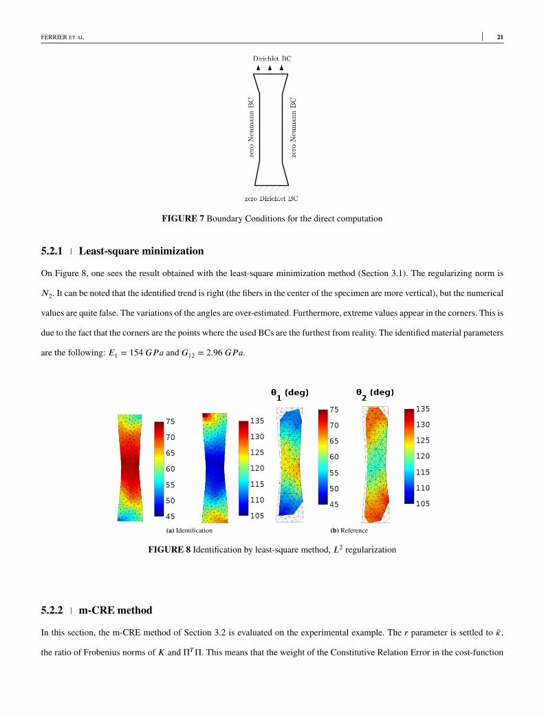
On Figure 8, one sees the result obtained with the least-square minimization method (Section 3.1). The regularizing norm is
N2. It can be noted that the identified trend is right (the fibers in the center of the specimen are more vertical), but the numerical
values are quite false. The variations of the angles are over-estimated. Furthermore, extreme values appear in the corners. This is
due to the fact that the corners are the points where the used BCs are the furthest from reality. The identified material parameters
are the following: E1 = 154 GPa and G12 = 2.96 GPa.
(a) Identification (b) Reference
FIGURE 8 Identification by least-square method, L2 regularization
5.2.2 m-CRE method
In this section, the m-CRE method of Section 3.2 is evaluated on the experimental example. The r parameter is settled to �,
the ratio of Frobenius norms of K and ΠTΠ. This means that the weight of the Constitutive Relation Error in the cost-function
22 FERRIER ET AL
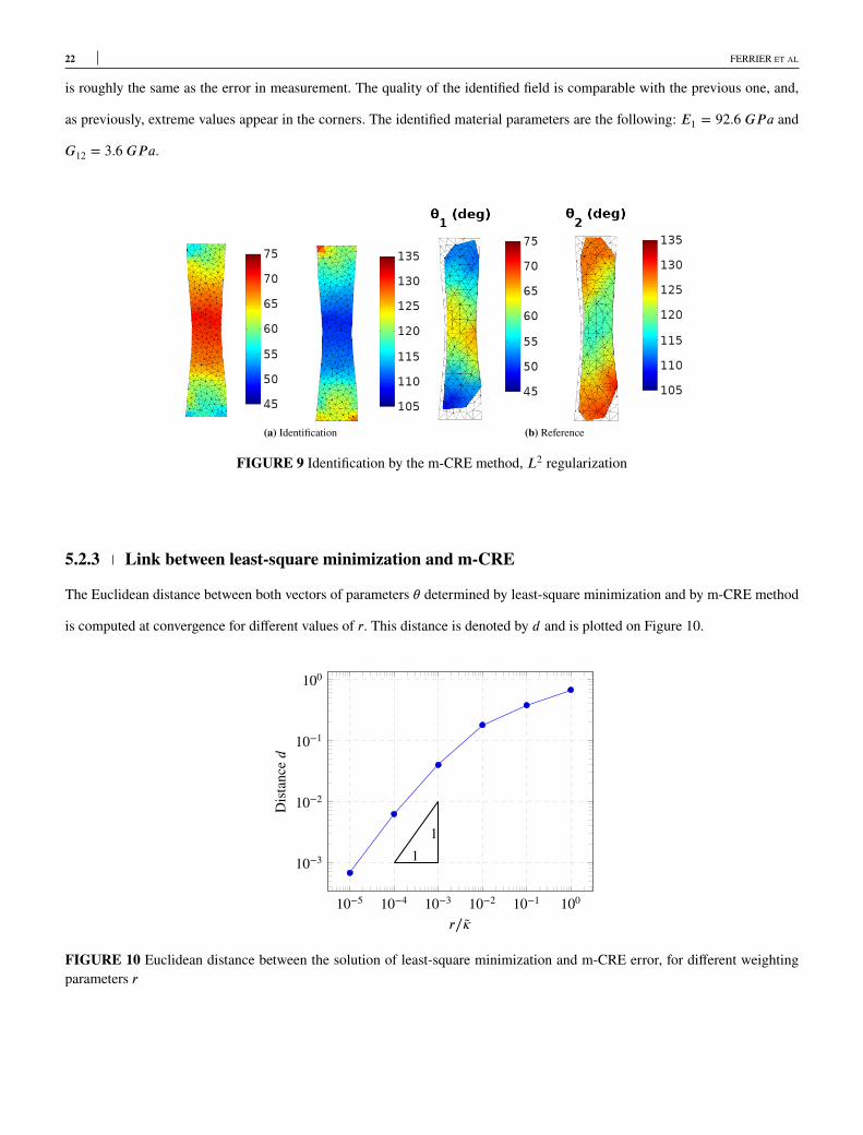
is roughly the same as the error in measurement. The quality of the identified field is comparable with the previous one, and,
as previously, extreme values appear in the corners. The identified material parameters are the following: E1 = 92.6 GPa and
G12 = 3.6 GPa.
(a) Identification (b) Reference
FIGURE 9 Identification by the m-CRE method, L2 regularization
5.2.3 Link between least-square minimization and m-CRE
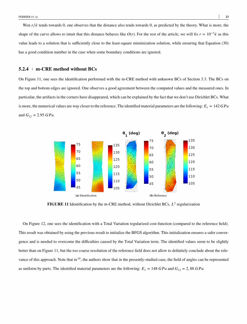
The Euclidean distance between both vectors of parameters � determined by least-square minimization and by m-CRE method
is computed at convergence for different values of r. This distance is denoted by d and is plotted on Figure 10.
10−5 10−4 10−3 10−2 10−1 100
10−3
10−2
10−1
100
11
r∕�
Distanced
FIGURE 10 Euclidean distance between the solution of least-square minimization and m-CRE error, for different weightingparameters r
FERRIER ET AL 23
Wen r∕� tends towards 0, one observes that the distance also tends towards 0, as predicted by the theory. What is more, the
shape of the curve allows to intuit that this distance behaves like O(r). For the rest of the article, we will fix r = 10−3� as this
value leads to a solution that is sufficiently close to the least-square minimization solution, while ensuring that Equation (30)
has a good condition number in the case when some boundary conditions are ignored.
5.2.4 m-CRE method without BCs
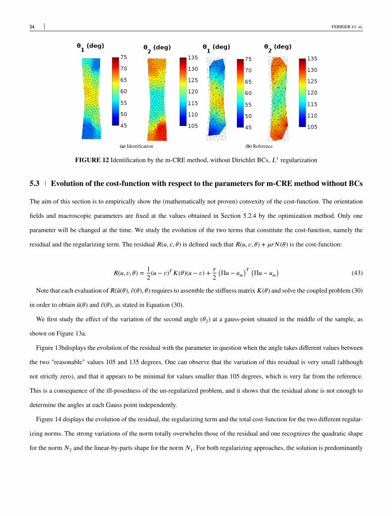
On Figure 11, one sees the identification performed with the m-CRE method with unknown BCs of Section 3.3. The BCs on
the top and bottom edges are ignored. One observes a good agreement between the computed values and the measured ones. In
particular, the artifacts in the corners have disappeared, which can be explained by the fact that we don’t use Dirichlet BCs. What
ismore, the numerical values areway closer to the reference. The identifiedmaterial parameters are the following:E1 = 142GPa
and G12 = 2.95 GPa.
(a) Identification (b) Reference
FIGURE 11 Identification by the m-CRE method, without Dirichlet BCs, L2 regularization
On Figure 12, one sees the identification with a Total Variation regularized cost-function (compared to the reference field).
This result was obtained by using the previous result to initialize the BFGS algorithm. This initialization ensures a safer conver-
gence and is needed to overcome the difficulties caused by the Total Variation term. The identified values seem to be slightly
better than on Figure 11, but the too coarse resolution of the reference field does not allow to definitely conclude about the rele-
vance of this approach. Note that in10, the authors show that in the presently-studied case, the field of angles can be represented
as uniform by parts. The identified material parameters are the following: E1 = 148 GPa and G12 = 2, 88 GPa.
24 FERRIER ET AL
(a) Identification (b) Reference
FIGURE 12 Identification by the m-CRE method, without Dirichlet BCs, L1 regularization
5.3 Evolution of the cost-function with respect to the parameters for m-CRE method without BCs
The aim of this section is to empirically show the (mathematically not proven) convexity of the cost-function. The orientation
fields and macroscopic parameters are fixed at the values obtained in Section 5.2.4 by the optimization method. Only one
parameter will be changed at the time. We study the evolution of the two terms that constitute the cost-function, namely the
residual and the regularizing term. The residual R(u, v, �) is defined such that R(u, v, �) + �rN(�) is the cost-function:
R(u, v, �) = 12(u − v)TK(�)(u − v) + r
2(
Πu − um)T (Πu − um
)
(43)
Note that each evaluation ofR(u(�), v(�), �) requires to assemble the stiffness matrixK(�) and solve the coupled problem (30)
in order to obtain u(�) and v(�), as stated in Equation (30).
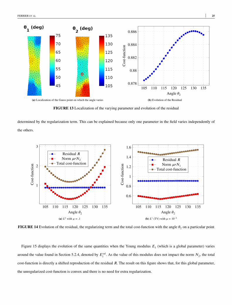
We first study the effect of the variation of the second angle (�2) at a gauss-point situated in the middle of the sample, as
shown on Figure 13a.
Figure 13bdisplays the evolution of the residual with the parameter in question when the angle takes different values between
the two "reasonable" values 105 and 135 degrees. One can observe that the variation of this residual is very small (although
not strictly zero), and that it appears to be minimal for values smaller than 105 degrees, which is very far from the reference.
This is a consequence of the ill-posedness of the un-regularized problem, and it shows that the residual alone is not enough to
determine the angles at each Gauss point independently.
Figure 14 displays the evolution of the residual, the regularizing term and the total cost-function for the two different regular-
izing norms. The strong variations of the norm totally overwhelm those of the residual and one recognizes the quadratic shape
for the normN2 and the linear-by-parts shape for the normN1. For both regularizing approaches, the solution is predominantly
FERRIER ET AL 25
(a) Localization of the Gauss point on which the angle varies
105 110 115 120 125 130 1350.878
0.88
0.882
0.884
0.886
Angle �2
Cost-functio
n
(b) Evolution of the Residual
FIGURE 13 Localization of the varying parameter and evolution of the residual
determined by the regularization term. This can be explained because only one parameter in the field varies independently of
the others.
105 110 115 120 125 130 135
1
2
3
Angle �2
Cost-functio
n
Residual RNorm �rN2
Total cost-function
(a) L2 with � = .1
105 110 115 120 125 130 135
0.6
0.8
1
1.2
1.4
1.6
Angle �2
Cost-functio
n
Residual RNorm �rN1
Total cost-function
(b) L1 (TV) with � = 10−4
FIGURE 14 Evolution of the residual, the regularizing term and the total cost-function with the angle �2 on a particular point
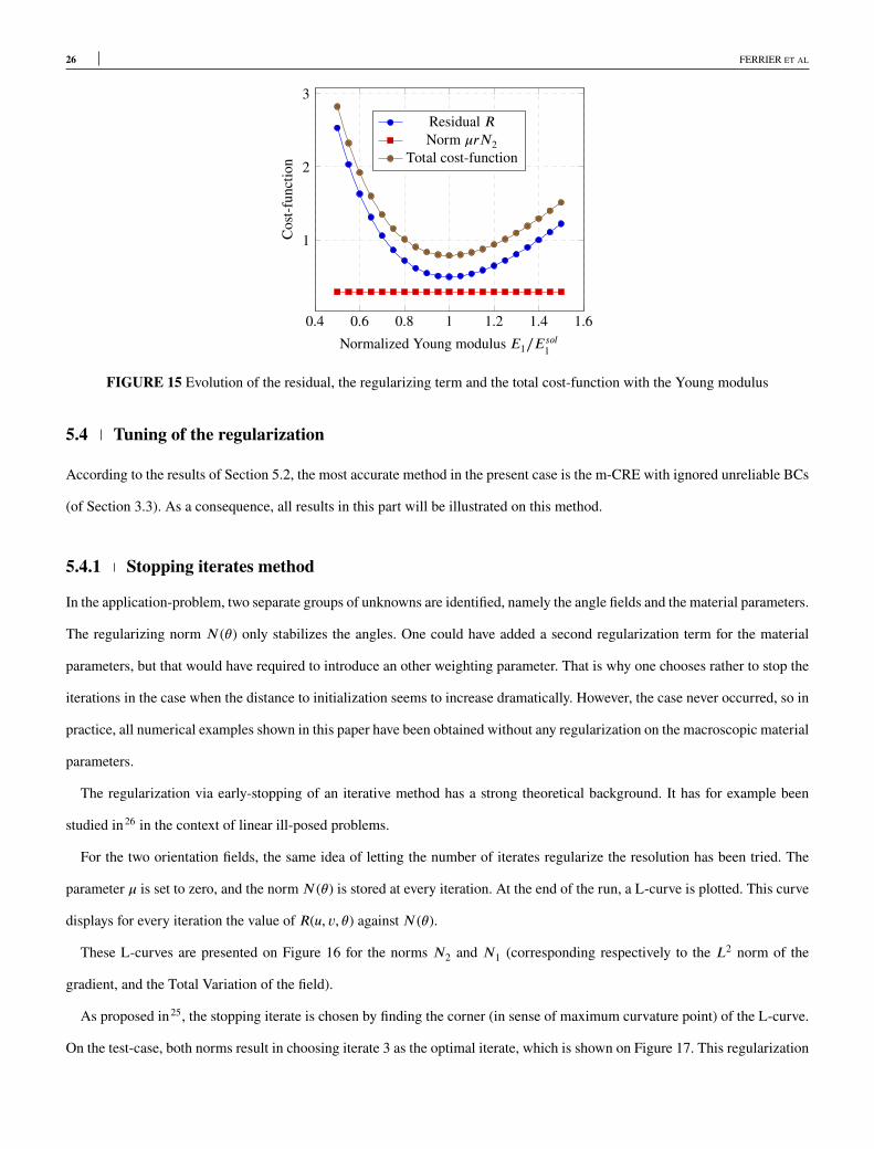
Figure 15 displays the evolution of the same quantities when the Young modulus E1 (which is a global parameter) varies
around the value found in Section 5.2.4, denoted by Esol1 . As the value of this modulus does not impact the norm N2, the total
cost-function is directly a shifted reproduction of the residual R. The result on this figure shows that, for this global parameter,
the unregularized cost-function is convex and there is no need for extra regularization.
26 FERRIER ET AL
0.4 0.6 0.8 1 1.2 1.4 1.6
1
2
3
Normalized Young modulus E1∕Esol1
Cost-functio
n
Residual RNorm �rN2
Total cost-function
FIGURE 15 Evolution of the residual, the regularizing term and the total cost-function with the Young modulus
5.4 Tuning of the regularization
According to the results of Section 5.2, the most accurate method in the present case is the m-CRE with ignored unreliable BCs
(of Section 3.3). As a consequence, all results in this part will be illustrated on this method.
5.4.1 Stopping iterates method
In the application-problem, two separate groups of unknowns are identified, namely the angle fields and the material parameters.
The regularizing norm N(�) only stabilizes the angles. One could have added a second regularization term for the material
parameters, but that would have required to introduce an other weighting parameter. That is why one chooses rather to stop the
iterations in the case when the distance to initialization seems to increase dramatically. However, the case never occurred, so in
practice, all numerical examples shown in this paper have been obtained without any regularization on the macroscopic material
parameters.
The regularization via early-stopping of an iterative method has a strong theoretical background. It has for example been
studied in26 in the context of linear ill-posed problems.
For the two orientation fields, the same idea of letting the number of iterates regularize the resolution has been tried. The
parameter � is set to zero, and the normN(�) is stored at every iteration. At the end of the run, a L-curve is plotted. This curve
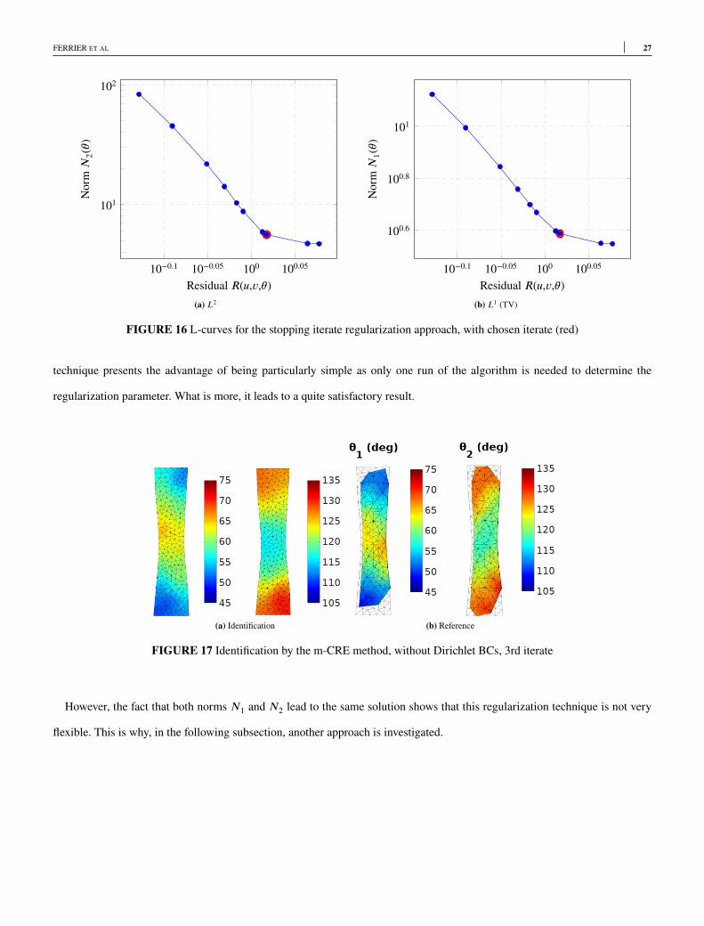
displays for every iteration the value of R(u, v, �) againstN(�).
These L-curves are presented on Figure 16 for the norms N2 and N1 (corresponding respectively to the L2 norm of the
gradient, and the Total Variation of the field).
As proposed in25, the stopping iterate is chosen by finding the corner (in sense of maximum curvature point) of the L-curve.
On the test-case, both norms result in choosing iterate 3 as the optimal iterate, which is shown on Figure 17. This regularization
FERRIER ET AL 27
10−0.1 10−0.05 100 100.05
101
102
Residual R(u,v,�)
NormN2(�)
(a) L2
10−0.1 10−0.05 100 100.05
100.6
100.8
101
Residual R(u,v,�)
NormN1(�)
(b) L1 (TV)
FIGURE 16 L-curves for the stopping iterate regularization approach, with chosen iterate (red)
technique presents the advantage of being particularly simple as only one run of the algorithm is needed to determine the
regularization parameter. What is more, it leads to a quite satisfactory result.
(a) Identification (b) Reference
FIGURE 17 Identification by the m-CRE method, without Dirichlet BCs, 3rd iterate
However, the fact that both norms N1 and N2 lead to the same solution shows that this regularization technique is not very
flexible. This is why, in the following subsection, another approach is investigated.
28 FERRIER ET AL
5.4.2 Tikhonov method
With this approach, and contrary to the stopping iterate method, the iterative minimization algorithm will be carried out until
convergence of the cost-function, and the regularization will come from the term N(�), and its weight, �. The key question is
to automatically identify a suitable value for this weight.
One manually identifies a "viable" interval of variation where the fields are not visually uniform, nor presenting high oscil-
lations. This interval is sampled, and we perform the inversion for several values of �. A L-curve is then plotted, that presents
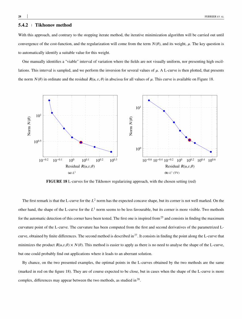
the normN(�) in ordinate and the residual R(u, v, �) in abscissa for all values of �. This curve is available on Figure 18.
10−0.2 10−0.1 100 100.1 100.2 100.3
100.5
101
Residual R(u,v,�)
NormN(�)
(a) L2
10−0.6 10−0.4 10−0.2 100 100.2 100.4 100.6
100
101
Residual R(u,v,�)
NormN(�)
(b) L1 (TV)
FIGURE 18 L-curves for the Tikhonov regularizing approach, with the chosen setting (red)
The first remark is that the L-curve for the L2 norm has the expected concave shape, but its corner is not well marked. On the
other hand, the shape of the L-curve for the L1 norm seems to be less favourable, but its corner is more visible. Two methods
for the automatic detection of this corner have been tested. The first one is inspired from25 and consists in finding the maximum
curvature point of the L-curve. The curvature has been computed from the first and second derivatives of the parametrized L-
curve, obtained by finite differences. The second method is described in27. It consists in finding the point along the L-curve that
minimizes the product R(u,v,�) ×N(�). This method is easier to apply as there is no need to analyse the shape of the L-curve,
but one could probably find out applications where it leads to an aberrant solution.
By chance, on the two presented examples, the optimal points in the L-curves obtained by the two methods are the same
(marked in red on the figure 18). They are of course expected to be close, but in cases when the shape of the L-curve is more
complex, differences may appear between the two methods, as studied in28.
FERRIER ET AL 29
When the L-curve is smooth, as it is the case here, it is possible to create a quadratic interpolation of the curvature around the
maximum curvature point in order to find an optimal value of � in the interval for which the interpolation has been performed.
By this means, we obtain � = .16 with the normN2 and � = 7.9 ⋅ 10−4 with the normN1.
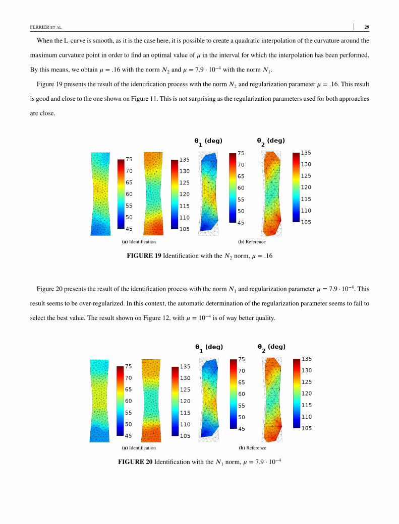
Figure 19 presents the result of the identification process with the normN2 and regularization parameter � = .16. This result
is good and close to the one shown on Figure 11. This is not surprising as the regularization parameters used for both approaches
are close.
(a) Identification (b) Reference
FIGURE 19 Identification with theN2 norm, � = .16
Figure 20 presents the result of the identification process with the normN1 and regularization parameter � = 7.9 ⋅ 10−4. This
result seems to be over-regularized. In this context, the automatic determination of the regularization parameter seems to fail to
select the best value. The result shown on Figure 12, with � = 10−4 is of way better quality.
(a) Identification (b) Reference
FIGURE 20 Identification with theN1 norm, � = 7.9 ⋅ 10−4
30 FERRIER ET AL
Another method for choosing the regularization parameter is the Morozov principle29, that presents the advantage of using
the information of the noise level on the measurement, and thus not to fall under the Bakushinkii veto30. When applied to the
m-CRE method, the Morozov principle consists in computing an expected value of the measurement mismatch m, from the
standard deviation on the measurement �, obtained in Section 2.2,m = �T �. We choose, among all values that have been tested
for �, the largest one that ensures(
Πu − um)T (Πu − um
)
⩽ m. In the present case, the Morozov principle would lead to � = .1
with the norm N2 and � = 5 ⋅ 10−4 with the norm N1. These results are close to those obtained by the L-curve method. This
confirms the coherence of the proposed methods for the choice of �.
All the values for � obtained with the three studied methods and for the two proposed regularizing terms are summarized in
Table 1.
Regularizing norm � maximum curvature � minimum product � MorozovL1 7.9 ⋅ 10−4 10−3 5 ⋅ 10−4
L2 .16 .1 .1
TABLE 1 Chosen values for � depending on the choice method
To conclude, in this numerical experiment, the different methods that have been tested to automatically determinate the
regularization parameter have given successful and coherent results when the normN2 is used. In the case of the normN1, the
results appear to be poorer. A possible explanation for this could have been that, due to the lack of utilization of a dedicated
algorithm, the L1-regularized cost-function optimization is inefficient. However, a numerical experimentation with the split
Bregman algorithm from22 led to the same outcome.
This is what led us to formulate another hypothesis: The L1 regularization shows poorer results because the test-case that
has been studied until now presents rather smooth variations of the parametric field on the whole domain. For this kind of
distribution, it can be expected that the L2 norm is better suited to identification.
5.4.3 Study of another test-case
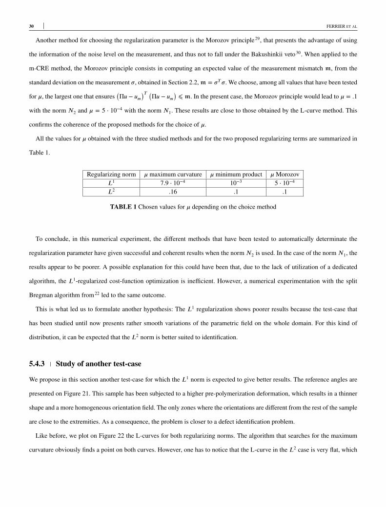
We propose in this section another test-case for which the L1 norm is expected to give better results. The reference angles are
presented on Figure 21. This sample has been subjected to a higher pre-polymerization deformation, which results in a thinner
shape and a more homogeneous orientation field. The only zones where the orientations are different from the rest of the sample
are close to the extremities. As a consequence, the problem is closer to a defect identification problem.
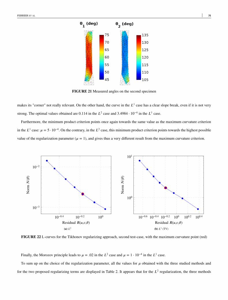
Like before, we plot on Figure 22 the L-curves for both regularizing norms. The algorithm that searches for the maximum
curvature obviously finds a point on both curves. However, one has to notice that the L-curve in the L2 case is very flat, which
FERRIER ET AL 31
FIGURE 21Measured angles on the second specimen
makes its "corner" not really relevant. On the other hand, the curve in the L1 case has a clear slope break, even if it is not very
strong. The optimal values obtained are 0.114 in the L2 case and 3.4984 ⋅ 10−4 in the L1 case.
Furthermore, the minimum product criterion points once again towards the same value as the maximum curvature criterion
in the L1 case: � = 5 ⋅ 10−4. On the contrary, in the L2 case, this minimum product criterion points towards the highest possible
value of the regularization parameter (� = 1), and gives thus a very different result from the maximum curvature criterion.
10−0.4 10−0.2 100
10−3
10−2
Residual R(u,v,�)
NormN(�)
(a) L2
10−0.6 10−0.4 10−0.2 100 100.2 100.4
100
101
Residual R(u,v,�)
NormN(�)
(b) L1 (TV)
FIGURE 22 L-curves for the Tikhonov regularizing approach, second test-case, with the maximum curvature point (red)
Finally, the Morozov principle leads to � = .02 in the L2 case and � = 1 ⋅ 10−4 in the L1 case.
To sum up on the choice of the regularization parameter, all the values for � obtained with the three studied methods and
for the two proposed regularizing terms are displayed in Table 2. It appears that for the L2 regularization, the three methods
32 FERRIER ET AL
give very different results. On the other hand, for the L1 regularization, the three methods lead to values that, although being
noticeably different, have the same order of magnitude.
Regularizing norm � maximum curvature � minimum product � MorozovL1 3.4984 ⋅ 10−4 5 ⋅ 10−4 10−4
L2 .114 1 (highest value tested) .02
TABLE 2 Chosen values for � depending on the choice method
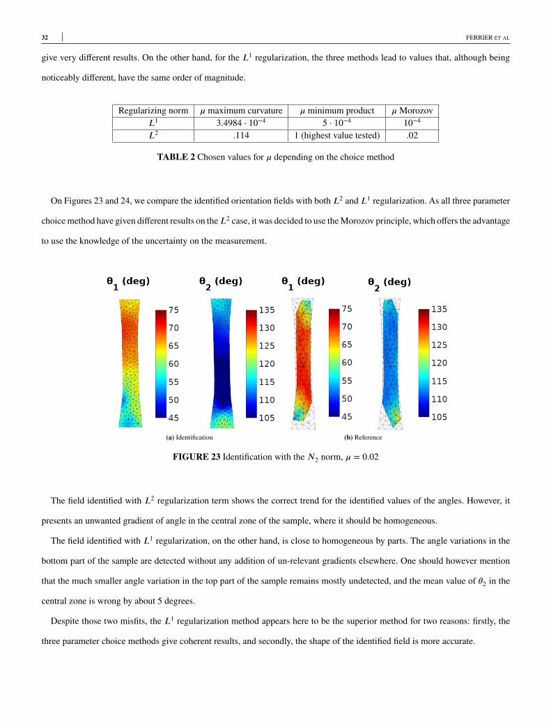
On Figures 23 and 24, we compare the identified orientation fields with both L2 and L1 regularization. As all three parameter
choicemethod have given different results on theL2 case, it was decided to use theMorozov principle, which offers the advantage
to use the knowledge of the uncertainty on the measurement.
(a) Identification (b) Reference
FIGURE 23 Identification with theN2 norm, � = 0.02
The field identified with L2 regularization term shows the correct trend for the identified values of the angles. However, it
presents an unwanted gradient of angle in the central zone of the sample, where it should be homogeneous.
The field identified with L1 regularization, on the other hand, is close to homogeneous by parts. The angle variations in the
bottom part of the sample are detected without any addition of un-relevant gradients elsewhere. One should however mention
that the much smaller angle variation in the top part of the sample remains mostly undetected, and the mean value of �2 in the
central zone is wrong by about 5 degrees.
Despite those two misfits, the L1 regularization method appears here to be the superior method for two reasons: firstly, the
three parameter choice methods give coherent results, and secondly, the shape of the identified field is more accurate.
FERRIER ET AL 33
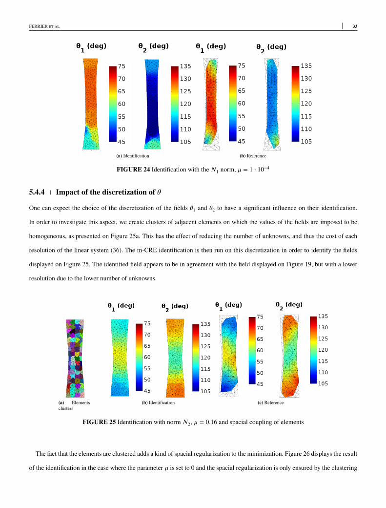
(a) Identification (b) Reference
FIGURE 24 Identification with theN1 norm, � = 1 ⋅ 10−4
5.4.4 Impact of the discretization of �
One can expect the choice of the discretization of the fields �1 and �2 to have a significant influence on their identification.
In order to investigate this aspect, we create clusters of adjacent elements on which the values of the fields are imposed to be
homogeneous, as presented on Figure 25a. This has the effect of reducing the number of unknowns, and thus the cost of each
resolution of the linear system (36). The m-CRE identification is then run on this discretization in order to identify the fields
displayed on Figure 25. The identified field appears to be in agreement with the field displayed on Figure 19, but with a lower
resolution due to the lower number of unknowns.
(a) Elementsclusters
(b) Identification (c) Reference
FIGURE 25 Identification with normN2, � = 0.16 and spacial coupling of elements
The fact that the elements are clustered adds a kind of spacial regularization to the minimization. Figure 26 displays the result
of the identification in the case where the parameter � is set to 0 and the spacial regularization is only ensured by the clustering
34 FERRIER ET AL
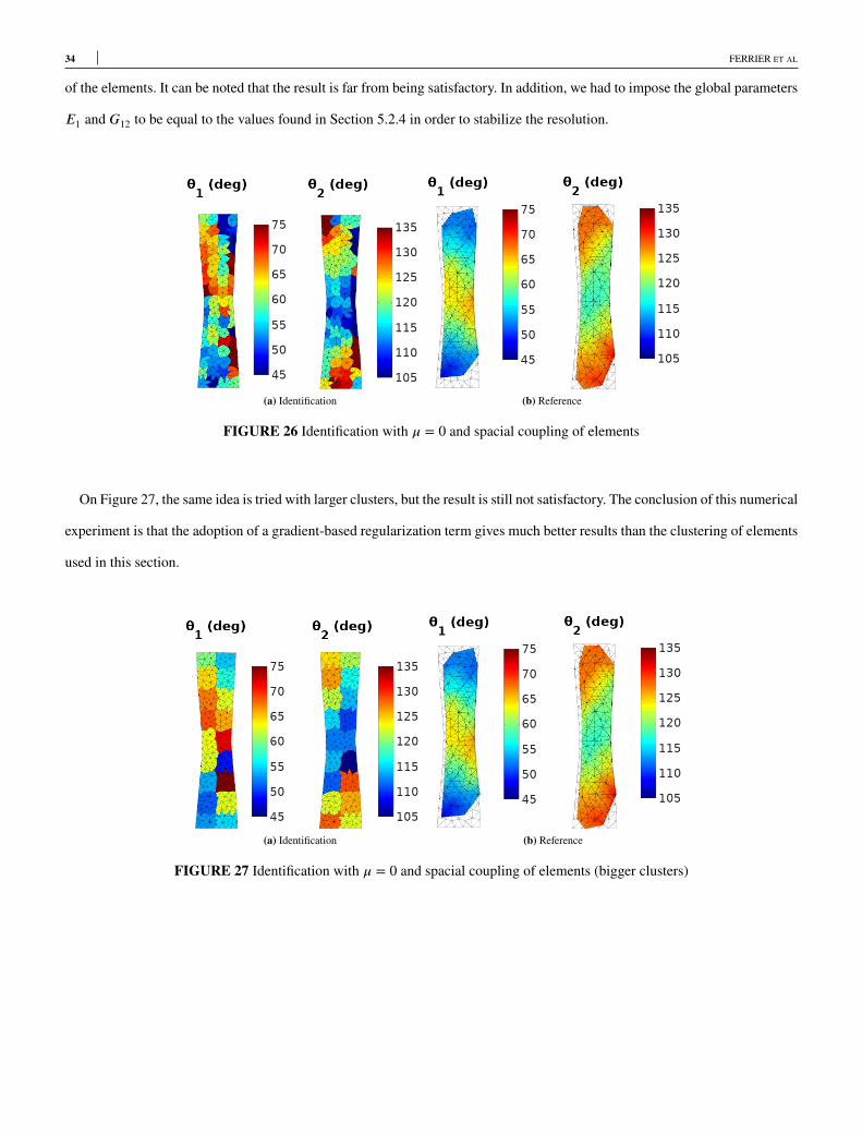
of the elements. It can be noted that the result is far from being satisfactory. In addition, we had to impose the global parameters
E1 and G12 to be equal to the values found in Section 5.2.4 in order to stabilize the resolution.
(a) Identification (b) Reference
FIGURE 26 Identification with � = 0 and spacial coupling of elements
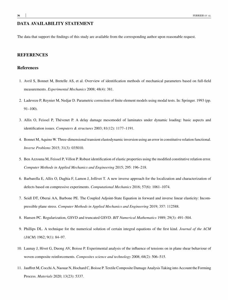
On Figure 27, the same idea is tried with larger clusters, but the result is still not satisfactory. The conclusion of this numerical
experiment is that the adoption of a gradient-based regularization term gives much better results than the clustering of elements
used in this section.
(a) Identification (b) Reference
FIGURE 27 Identification with � = 0 and spacial coupling of elements (bigger clusters)

FERRIER ET AL 35
6 CONCLUSION
In this study, two variants of the modified Constitutive Relation Error method have been studied both theoretically and
numerically, and compared to another classical method, namely the PDE-constrained optimization, on an experimental test-case.
All theoretical developments done in this paper have been confronted with experimental measurements. The test-problem
consists in the identification of the inhomogeneous orientation of the fibers of a composite specimen from full-field displacement
measurement. As the global stiffness parameters of the studied material are only roughly known, this experiment enabled us to
test the identification of a few global parameters along with the parametric fields. Such an identification method has proven to
converge well.
It was shown that the use of a norm of the gradient of the identified field is an interesting way to enhance the quality of the
identification with the m-CRE method. A term proportional to this norm can either be directly added to the function that is
minimized, or it can serve as an ingredient of a regularizing stopping criterion. Two norms of the gradient have been tested, in
order to illustrate the fact that while the L2-regularized solution is smooth on the whole domain, the L1-regularized solution
tends to have rather homogeneous zones, separated by sharp frontiers. The choice between L1 and L2 norms is meant to be
made from the a priori knowledge of the shape of the identified field.
The automatic determination of the two parameters of the method is a critical point in the perspective of designing black-
box tools for identification. For this purpose, we proposed to impose the weighting parameter to take an arbitrary value that
is small compared to a particular ratio of spectral radii. In that case, the proposed method can then simply be interpreted as a
generalization of the least-square minimization method in order not to be forced to use unreliable BCs on the domain. For the
determination of the regularization parameter, both L-curve and Morozov method have been tested.
Two different test-cases have been investigated. The L2-regularized cost-function seems better suited to the first one, for
which the field to identify has smooth gradients. The second test-case presents a large homogeneous zone and sharp variations
of the field at its extremities and turns out to be overall more challenging. It seems to be better handled by the L1-regularized
cost-function. This investigation highlights the fact that the two proposed regularization terms are best applied to different
test-cases.
Two main perspectives emerge from this study. The first one concerns the application of the method to dynamics problems,
that are known to be more opportune for the identification, in order to identify a full heterogeneous field of orthotropic stiffness
parameters of the material. The second perspective is the acceleration of the computation. The fact that many similar direct
resolutions have to be performed in order to identify the parameters has led many authors to propose the use of a reduced order
model, like in31. In our case, the reduction method has to be able to deal with a field of parameters, as does the method presented
in32.
36 FERRIER ET AL
DATA AVAILABILITY STATEMENT
The data that support the findings of this study are available from the corresponding author upon reasonable request.
REFERENCES
References
1. Avril S, Bonnet M, Bretelle AS, et al. Overview of identification methods of mechanical parameters based on full-field
measurements. Experimental Mechanics 2008; 48(4): 381.
2. Ladeveze P, Reynier M, Nedjar D. Parametric correction of finite element models using modal tests. In: Springer. 1993 (pp.
91–100).
3. Allix O, Feissel P, Thévenet P. A delay damage mesomodel of laminates under dynamic loading: basic aspects and
identification issues. Computers & structures 2003; 81(12): 1177–1191.
4. BonnetM, AquinoW. Three-dimensional transient elastodynamic inversion using an error in constitutive relation functional.
Inverse Problems 2015; 31(3): 035010.
5. Ben AzzounaM, Feissel P, Villon P. Robust identification of elastic properties using the modified constitutive relation error.
Computer Methods in Applied Mechanics and Engineering 2015; 295: 196–218.
6. Barbarella E, Allix O, Daghia F, Lamon J, Jollivet T. A new inverse approach for the localization and characterization of
defects based on compressive experiments. Computational Mechanics 2016; 57(6): 1061–1074.
7. Seidl DT, Oberai AA, Barbone PE. The Coupled Adjoint-State Equation in forward and inverse linear elasticity: Incom-
pressible plane stress. Computer Methods in Applied Mechanics and Engineering 2019; 357: 112588.
8. Hansen PC. Regularization, GSVD and truncated GSVD. BIT Numerical Mathematics 1989; 29(3): 491–504.
9. Phillips DL. A technique for the numerical solution of certain integral equations of the first kind. Journal of the ACM
(JACM) 1962; 9(1): 84–97.
10. Launay J, Hivet G, Duong AV, Boisse P. Experimental analysis of the influence of tensions on in plane shear behaviour of
woven composite reinforcements. Composites science and technology 2008; 68(2): 506–515.
11. JauffretM, Cocchi A,NaouarN,HochardC, Boisse P. Textile Composite DamageAnalysis Taking intoAccount the Forming
Process. Materials 2020; 13(23): 5337.
FERRIER ET AL 37
12. ARAMIS . ℎttp ∶ ∕∕www.gom.com. GOM . 2015.
13. Gay D. Composite materials: design and applications. CRC press . 2014.
14. Banerjee B, Walsh TF, Aquino W, Bonnet M. Large scale parameter estimation problems in frequency-domain elastody-
namics using an error in constitutive equation functional. Computer methods in applied mechanics and engineering 2013;
253: 60–72.
15. Guo J, Wang L, Takewaki I. Frequency response-based damage identification in frames by minimum constitutive relation
error and sparse regularization. Journal of Sound and Vibration 2019; 443: 270–292.
16. Aquino W, Bonnet M. Analysis of the error in constitutive equation approach for time-harmonic elasticity imaging. SIAM
Journal on Applied Mathematics 2019; 79(3): 822–849.
17. Caillé L, Hanus J, Delvare F, Michaux-Leblond N. MFS fading regularization method for the identification of boundary
conditions from partial elastic displacement field data. European Journal of Computational Mechanics 2018; 27(5-6): 508–
539.
18. Fletcher R. A new approach to variable metric algorithms. The computer journal 1970; 13(3): 317–322.
19. Chan TF, Golub GH, Mulet P. A nonlinear primal-dual method for total variation-based image restoration. SIAM journal
on scientific computing 1999; 20(6): 1964–1977.
20. Mascareñas D, Cattaneo A, Theiler J, Farrar C. Compressed sensing techniques for detecting damage in structures.
Structural Health Monitoring 2013; 12(4): 325–338.
21. Zhang Z, Xu Y, Yang J, Li X, Zhang D. A survey of sparse representation: algorithms and applications. IEEE access 2015;
3: 490–530.
22. Goldstein T, Osher S. The split Bregman method for L1-regularized problems. SIAM journal on imaging sciences 2009;
2(2): 323–343.
23. Chamoin L, Ladevèze P, Waeytens J. Goal-oriented updating of mechanical models using the adjoint framework. Compu-
tational mechanics 2014; 54(6): 1415–1430.
24. Miller K. Least squares methods for ill-posed problems with a prescribed bound. SIAM Journal on Mathematical Analysis
1970; 1(1): 52–74.
25. Hansen PC. Analysis of discrete ill-posed problems by means of the L-curve. SIAM review 1992; 34(4): 561–580.

38 FERRIER ET AL
26. Santos RJ. Equivalence of regularization and truncated iteration for general ill-posed problems. Linear algebra and its
applications 1996; 236: 25–33.
27. Regińska T. A regularization parameter in discrete ill-posed problems. SIAM Journal on Scientific Computing 1996; 17(3):
740–749.
28. Johnston PR, Gulrajani RM. Selecting the corner in the L-curve approach to Tikhonov regularization. IEEE Transactions
on biomedical engineering 2000; 47(9): 1293–1296.
29. Morozov VA. The error principle in the solution of operational equations by the regularization method. Zhurnal Vychisli-
tel’noi Matematiki i Matematicheskoi Fiziki 1968; 8(2): 295–309.
30. Bakushinskii A. Remarks on choosing a regularization parameter using the quasioptimality and ratio criterion. USSR
Computational Mathematics and Mathematical Physics 1985; 24(4): 181–182.
31. Marchand B, Chamoin L, Rey C. Real-time updating of structural mechanics models using Kalman filtering, modified con-
stitutive relation error, and proper generalized decomposition. International Journal for Numerical Methods in Engineering
2016; 107(9): 786–810.
32. Paillet C, Néron D, Ladevèze P. A door to model reduction in high-dimensional parameter space. Comptes Rendus
Mécanique 2018; 346(7): 524–531.
Related Documents