Modern Technologies for Design Data Collection

21-1 08/05 JTRP-2003/13 INDOT Division of Research West Lafayette, IN 47906

INDOT Research

TECHNICAL Summary Technology Transfer and Project Implementation Information

TRB Subject Code: 21-1 Aerial and Ground Surveys August 2005 Publication No.: FHWA/IN/JTRP-2003/13, SPR-2450 Final Report Modern Technologies for Design Data Collection

Introduction The need for this research was motivated by the realizations that (1) field data collection is a very time consuming, labor intensive and error prone activity, and that (2) this is a field of frenetic research and development efforts by commercial equipment manufacturers and by academic researchers. A prudent organization would reassess their data collection methods every few years to permit them to take advantage of advances and innovations in the technology. Particular attention will be paid to issues of database formats, CAD data formats, and other software standards so that any data sets

produced would be compatible with existing analysis tools. Nevertheless, to look ahead, we will suggest some likely candidates for consideration when the decisions are eventually made about which areas of measurement and data collection technology appear to be the most promising. The project is aiming at intelligent selection and evaluation of recently developed and improved methods to collect or use geospatial data in order to be adopted by the Indiana Department of Transportation (INDOT) for the sake of higher level of efficiency regarding content, accuracy, effort, time and cost.

Findings The results of this project are as follows:

1) A terrestrial Lidar survey provides an efficient and timely tool to generate data for as-built surveys and engineering design.

2) The Lidar survey acquired the same accuracy as classical survey data collection methods: aerial photogrammetry in combination with terrestrial surveys.

3) The Lidar survey requires careful planning as to the still needed control surveys. Once the control surveys are in place Lidar surveys equal classical survey techniques in accuracy, but outperform them in timeliness.

4) The Lidar survey as applied to two bridges over the Interstate I-70 provided models within 48 hours. This period includes lidar data collection and analysis.

Implementation Lidar surveys can immediately implemented as part of standard survey operations for as-built and design applications. The technique is accurate with proper control and very timely. The technique has the portential to contribute substantially to so-called virtual survey office models whereby costly trips back to the field are avoided. Changed insights in survey

parameter extraction do not require return to the field either. Since Lidar is basically a line-of-sight technique possible obstruction may occur. Hence planning of Lidar surveys does not only include the necessary control for correct geopositioning of point clouds but also careful planning of Lidar system set-ups to avoid line-of-sight obstruction.


Contacts For more information: Prof. Boudewijn H.W. van Gelder Principal Investigator School of Civil Engineering Purdue University West Lafayette IN 47907 Phone: (765) 494-2165 Fax: (765) 496-1105 E-mail: [email protected] Prof. James S. Bethel Principal Investigator School of Civil Engineering Purdue University West Lafayette IN 47907 Phone: (765) 494-6719 Fax: (765) 496-1105 E-mail: [email protected]

Indiana Department of Transportation Division of Research 1205 Montgomery Street P.O. Box 2279 West Lafayette, IN 47906 Phone: (765) 463-1521 Fax: (765) 497-1665 Purdue University Joint Transportation Research Program School of Civil Engineering West Lafayette, IN 47907-1284 Phone: (765) 494-9310 Fax: (765) 496-7996


Summary and Highlights of Results

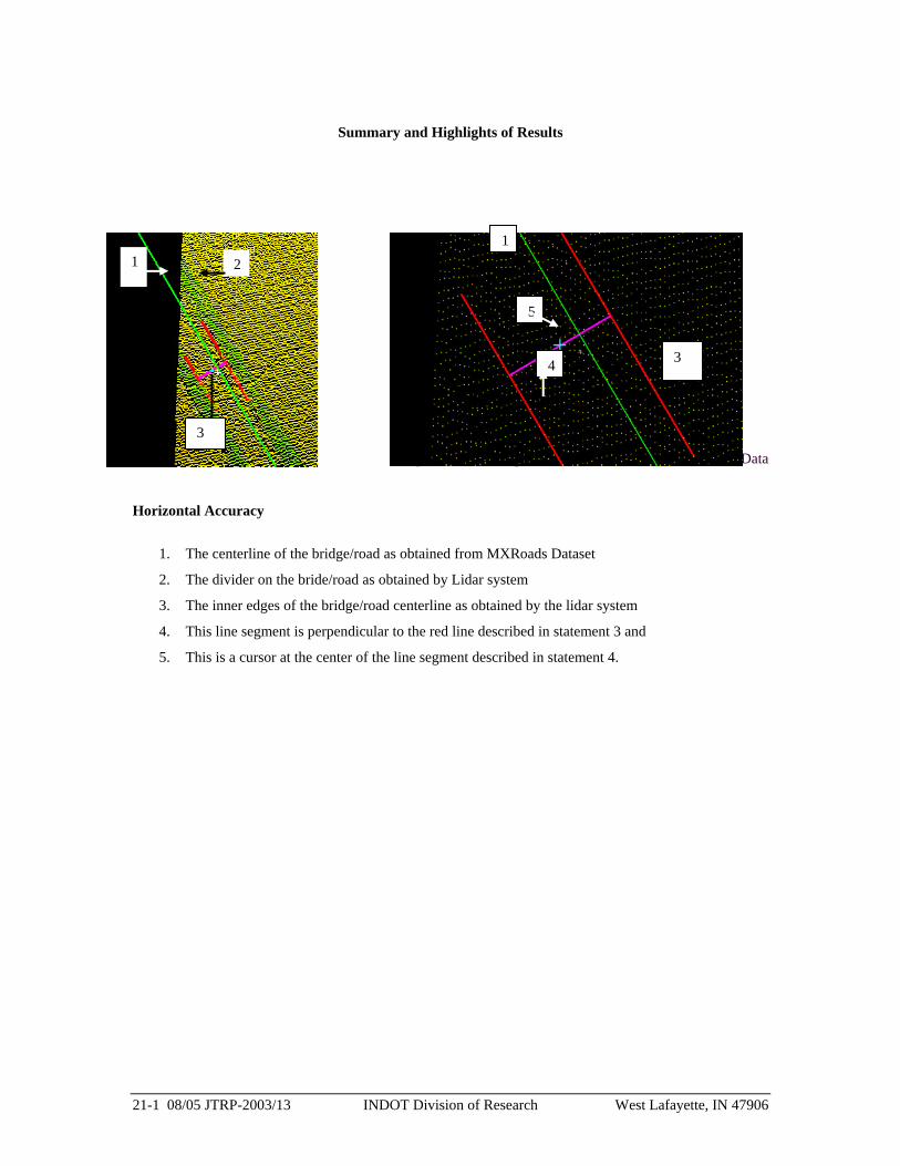
Figures 1a, b. Comparison of Lidar Scan with MXRoads Data

Horizontal Accuracy

1. The centerline of the bridge/road as obtained from MXRoads Dataset

2. The divider on the bride/road as obtained by Lidar system

3. The inner edges of the bridge/road centerline as obtained by the lidar system

4. This line segment is perpendicular to the red line described in statement 3 and

5. This is a cursor at the center of the line segment described in statement 4.

1 2

3

1

3 4

5


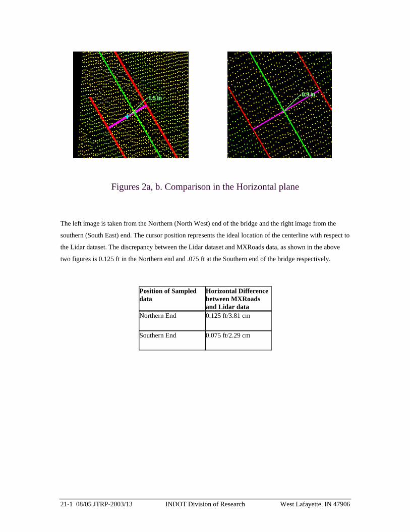
Figures 2a, b. Comparison in the Horizontal plane

The left image is taken from the Northern (North West) end of the bridge and the right image from the

southern (South East) end. The cursor position represents the ideal location of the centerline with respect to

the Lidar dataset. The discrepancy between the Lidar dataset and MXRoads data, as shown in the above

two figures is 0.125 ft in the Northern end and .075 ft at the Southern end of the bridge respectively.

Position of Sampled data

Horizontal Difference between MXRoads and Lidar data

Northern End 0.125 ft/3.81 cm

Southern End 0.075 ft/2.29 cm


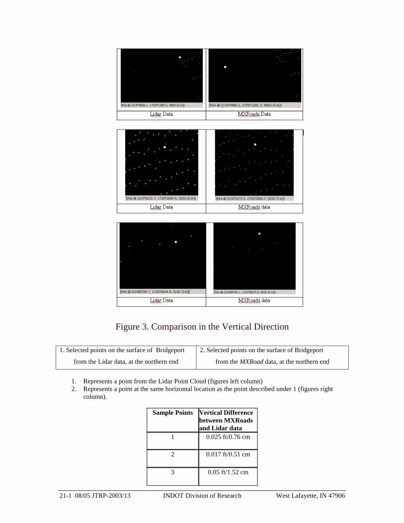
Figure 3. Comparison in the Vertical Direction

1. Represents a point from the Lidar Point Cloud (figures left column) 2. Represents a point at the same horizontal location as the point described under 1 (figures right

column).

Sample Points Vertical Difference between MXRoads and Lidar data

1 0.025 ft/0.76 cm

2 0.017 ft/0.51 cm

3 0.05 ft/1.52 cm

1. Selected points on the surface of Bridgeport

from the Lidar data, at the northern end

2. Selected points on the surface of Bridgeport

from the MXRoad data, at the northern end


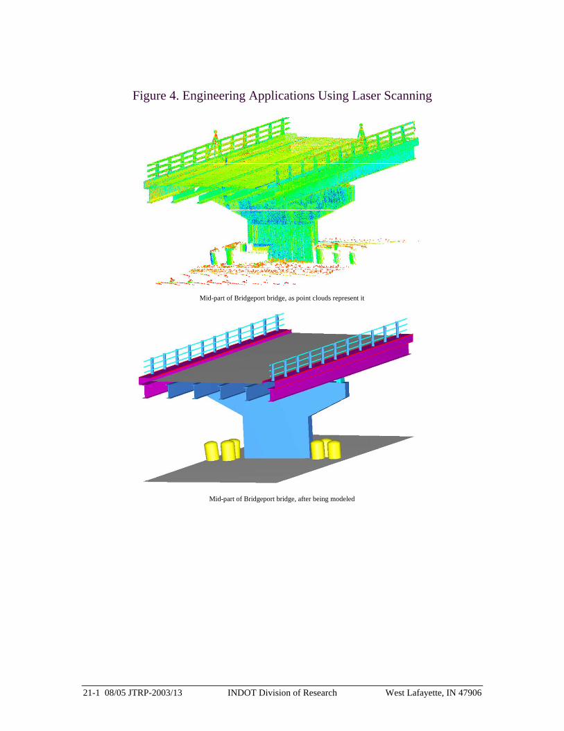
Figure 4. Engineering Applications Using Laser Scanning

Mid-part of Bridgeport bridge, as point clouds represent it

Mid-part of Bridgeport bridge, after being modeled

TECHNICAL REPORT STANDARD TITLE PAGE

1. Report No. FWHA/IN/JTRP-2003/13

2. Government Accession No. 3.Recipient’s Catalog No.

5.Report Date

4. Title and Subtitle

Modern Technologies for Design Data Collection 6.Performing Organization Code

7. Author(s) James S. Bethel, Steven D. Johnson, Jie Shan, Boudewijn H.W. van Gelder, Bob McCullouch, Ali Fuat Cetin, Seungwoo Han, Mosab Hawarey, Changno Lee, Aparajithan Sampath

8. Performing Organization Report No. FWHA/IN/JTRP-2003/13

10. Work Unit No.

9. Performing Organization Name and Address Joint Transportation Research Program School of Civil Engineering Purdue University 550 Stadium Mall West Lafayette, IN 47907-2051

11. Contract or Grant No. SPR-2450 13. Type of Report and Period Covered Final Report

12. Sponsoring Agency Name and Address Indiana Department of Transportation State Office Building 100 North Senate Avenue Indianapolis, IN 46204 14. Sponsoring Agency Code 15. Supplementary Notes 16. Abstract

Design data collection involving the use of Lidar instrument, in conjunction with GPS proves to be very effective. Data required to model two bridges over the I-70 was collected on a single day, involving five and six sessions with Lidar equipment. Even though the data was collected on two bridges, it did not cause any disruption of the traffic, either on the Interstate or on the bridges. A major cause of concern during survey activities, particularly along interstates is safety, both for the motorists as well as the people involved in data collection. Lidar data collection was found to be extremely safe in both aspects.

The whole process of collecting Lidar data and GPS coordinates for control was completed in 2 days for both bridges. Office work involved combining the GPS data with conventional survey data to bring control on six pre-selected points within the Lidar point cloud. This control information was later used to bring the point cloud into a geographic coordinate system.

This survey provided the means to compare the 3D point cloud with bridge designs that were created using other methods of data collection. It was found that the 3D point cloud exhibits a very high degree of accuracy, both internally and also when geo-referenced independently using GPS and conventional control survey. The Lidar model was compared to the MXRoad data model provided by INDOT. The discrepancies between the two models were not larger than 0.125 ft/3.81 cm horizontally and 0.05 ft/1.52 cm vertically.

The data collected completely modeled the bridge and the accuracy of the data ensures that any model of the bridge, either as a whole or in part, will correctly reflect the current state of the bridge. The data collected can also be used for various applications including cut-and-fill estimates, modeling the state of the bridge, making measurements on various parts of the bridge.

A cause of concern is the amount of data involved. As millions of 3D points are collected, popular CAD/GIS packages are unable to deal with it. For this reason proprietary software, designed particularly to handle such huge volumes of data involved, was used for analyzing this data. However, it is possible to export data from this software to other commonly used CAD packages. Using satellite imagery instead of aerial photos may provide faster results to investigate the project area. Conversion of the MXROAD data into the ArcGIS system is not easy, but it is hoped that this problem can be solved very easily. The Lidar point cloud should be processed and a CAD model of the data should be obtained to obtain more useful information. With the help of the GIS a variety of data sources and types can be integrated, visualized and used to make about resource management, and perform modeling and analysis. GIS helps organize bridge management information contained in various forms, such as inspection reports, rehab plans, and CAD files. Maintenance management and asset valuation may be enhanced with GIS and linear referencing systems. 17. Keywords Lidar, GPS, GIS, Satellite Imagery, Control, Design Software

18. Distribution Statement

19. Security Classf. (of this report) 20. Security Classf. (of this page) 21. No. Of Pages 130

22. Price

Form DOT F 1700.7 (8-69)

iii

ACKNOWLEDGEMENTS

The inputs of the members of the two Study Advisory Committees are gratefully acknowledged: SAC1: Karen Zhu, Michael Andrews, Mark Burton, Rick Yunker, and Anthony DeSimone; SAC2: Karen Zhu, Jim Nugent, Mark Burton, Rick Yunker, and Anthony DeSimone. William A. Schmidt (INDOT Design Division) was helpful during the project selection phase. Bill Schmidt’s workshop on MX Roads at Purdue University to the researchers in this project is greatly appreciated.

v

TABLE OF CONTENTS

Page

CHAPTER 1. Introduction

1

CHAPTER 2. Technologies vs. Design Software

2.1 Construction Data Collection

2.2 Cost Analysis

2.3 Highway Design Software

3

3

3

4

CHAPTER 3. Laser Scanning

3.1 Introduction

3.2 Optech Survey

3.3 Falk PLI Survey

3.4 Time taken for Data Collection

3.5 Alignment with MXRoad data

3.6 Test Laser Scan at US 52 – Northwestern Avenue

3.7 Engineering Applications

3.8 System Requirements

11

11

12

16

21

21

29

30

35

CHAPTER 4. Satellite Imagery (QuickBird Image Rectification)

4.1 Summary

4.2 Original Image

4.3 Ground Control Points

4.4 Linear Transformation Model

4.5 Non-Linear Sensor Model

4.6 Image Resection

4.7 Rectification Grid

4.8 Image Rectification

4.9 Potential Improvements

37

37

38

40

40

42

42

44

44

44

CHAPTER 5. Control

1.1 Global Positioning System (GPS)

1.2 Data Processing

1.2.1 Processing the Data in MOVE3

46

46

63

63

vi

1.2.2 The Adjustment

1.2.3 Ellipsoidal Heights to Ortho-metric Heights

65

67

CHAPTER 6. Geographic Information System (GIS)

6.1 Introduction

6.2 Data

6.3 Methodology

6.3.1 Data Processing

6.3.2 3D Modeling and Analysis

6.4 Results

68

68

69

75

75

77

81

CHAPTER 7. Conclusions 82

APPENDIX A CDROM_Lidar Movies

APPENDIX B GIS Movie

APPENDIX C GPS Analysis

APPENDIX D MOVE3 Analysis

APPENDIX E Diagnostics of Registration within Cyclone

APPENDIX F Powerpoint Presentation

REFERENCES

84

85

86

102

126

129

130

vii

LIST OF TABLES

Page

Table 2.1. The Comparison with Highway Design Software Used in US State

DOT’s

5

Table 2.2. Legend for Table 2.1 10

Table 3.1 Part of registration diagnostics report 19

Table 3.2 Volume of soil under I-70 and embankments at sample depth values

34

Table 3.3 Clearance values of Bridgeport bridge over I-70 at sample intervals 36

Table 4.1 Geodetic coordinates of the nine control points 40

Table 4.2 Resulting Residuals for Each Control Point 41

Table 4.3 Resection Values 43

Table 5.1 Order of Control Points (source: www.ngs.noaa.gov) 48

Table 5.2 GPS Survey Design 53

Table 5.3 GPS Survey Stations and Sessions 56

Table 5.4 Final Results of Adjusted Coordinates in NAD83 60

Table 5.5 Results of Adjustment in Geographic Coordinates 66

Table 5.6 Results of Adjustment in UTM Coordinates 66

Table 5.7 Results of Adjustment in State Plane Coordinates 66

viii

LIST OF FIGURES Page

Figure 1. Comparison of Lidar Scan with MXRoads Data ii

Figure 2. Comparison in the Horizontal plane iii

Figure 3. Comparison in the Vertical Direction iv

Figure 4. Engineering Applications Using Laser Scanning v

Figure 3.1 The scope of Optech’s twelve scans of Bridgeport bridge.

Figure 3.2 The ILRIS-3D laser scanner

Figure 3.3 The first scan in Figure 3.1 as appears in Polyworks’ viewer only

version

Figure 3.4 Image of Bridgeport bridge and 3 zoomed images, as scanned by

ILRIS-3D

Figure 3.5 Special tripod for Cyrax 2500

Figure 3.6 Snapshot of a scan taken from the east of Bridgeport bridge

Figure 3.7 Semi-spheres scanned by Cyrax 2500 and to be modeled by

Cyclone, on Bridgeport bridge

Figure 3.8 Sphere mounted on tripod, modeled to serve as control point

Figure 3.9 Symmetry of control points

Figure 3.10 Sample error when registering all point clouds to GPS coordinates

Figure 3.11 Bridgeport bridge registered to GPS coordinates, with 4 zoomed in

images

Figure 3.12 Data imported from MXRoad

Figure 3.13 Bridgeport bridge as in the data imported from MXRoad

Figure 3.14 Vertical control point of G163 on Bridgeport bridge

Figure 3.15 Point clouds of laser scanning correctly geo-positioned onto

MXRoad data

Figure 3.16 Good overlap of lidar data on MXRoad data across the I-70

Figure 3.17 Confirmation of the good overlap of lidar data on MXRoad data

across the I-70

Figure 3.18 Good overlap of lidar data on MXRoad data across Bridgeport

bridge

12

13

13

14

16

16

17

17

18

18

19

22

22

23

23

24

24

25

ix

Figure 3.19 Confirmation of the good overlap of lidar data on MXRoad data

across Bridgeport bridge

Figure 3.20 Curvature of the Bridgeport road surface, represented by lidar data

Figure 3.21 Magnified image of northern end

Figure 3.22 Figure 3.21 magnified further more

Figure 3.23 Discrepancy between MXRoad’s centerline and lidar’s centerline

at northern end

Figure 3.24 Discrepancy between MXRoad’s centerline and lidar’s centerline

at southern end

Figure 3.25 Picked point on the surface of I-70 from the lidar data

Figure 3.26 Picked point on the surface of I-70 from the MXRoad data

Figure 3.27 Picked point on the surface of Bridgeport from the lidar data, at the

northern end

Figure 3.28 Picked point on the surface of Bridgeport from the MXRoad data,

at the northern end

Figure 3.29 Picked point on the surface of Bridgeport from the lidar data, at the

southern end

Figure 3.30 Picked point on the surface of Bridgeport from the MXRoad data,

at the southern end

Figure 3.31 Northwestern Avenue’s bridge on US 52 in West Lafayette, IN

Figure 3.32 Mid-part of Bridgeport bridge, as point clouds represent it

Figure 3.33 Mid-part of Bridgeport bridge, after being modeled

Figure 3.34 The volume of modeled 3D bridge pillar

Figure 3.35 Meshed surfaces and elevation contours

Figure 3.36 Volume between mesh and reference plane

Figure 3.37 Example sketch of bridge clearances

Figure 3.38 Bridgeport bridge clearance over I-70

25

26

27

27

27

27

28

28

28

28

28

28

29

31

31

32

33

34

35

36

Figure 4.1 Rectified Satellite imagery

Figure 4.2 Original Satellite Imagery

38

39

Figure 5.1 Map of KA0140


47

47

x



Figure 5.5 Control points around the project area and the bridge locations

Figure 5.6 The selected control points around the project area and the bridges.

Figure 5.7 NGS Control Point: KA0140 (Mills Reset)

Figure 5.8 Measurement of Approximate Coordinates of KA0140

Figure 5.9 NGS Control Point: KA1653 (F 350)

Figure 5.10 NGS Control Point: KA0159 (C 64)

Figure 5.11 Easy Accessibility to Point KA0159

Figure 5.12 NGS Control Point KA1958 (Plain)

Figure 5.13 Point KA1958 in the Hole

Figure 5.14 Design map with paths between the points showing the distances

Figure 5.15 Bridgeport Bridge

Figure 5.16 GPS Survey

Figure 5.17 GPS Survey

Figure 5.18 Six Points Bridge

Figure 5.19 Occupation View

Figure 5.20 Free Network Adjustment Results

Figure 5.21 Area of Pilot Project

Figure 5.22 Bridgeport bridge

Figure 5.23 Six Point bridge

Figure 5.24 Layout of Points on the Bridgeport Bridge

Figure 5.25 Total Station Survey

Figure 5.26 Total Station Survey

48

48

48

49

49

50

50

51

51

52

52

54

55

56

56

57

58

59

59

60

60

62

63

63

Figure 6.1 A part of the DOQs showing the project area

Figure 6.2 NED DEM data for the project area

Figure 6.3 A portion of the satellite photo showing the project area

Figure 6.4 MXROAD data used in the project

Figure 6.5 Lidar data showing the bridge

Figure 6.6 The data used in the project

Figure 6.7 3D Model showing the MXROAD data, DOQs, satellite imagery

69

71

73

74

75

77

xi

and the DEM

Figure 6.8 MXROAD data can be queried in ArcScene environment

Figure 6.9 Comparison of the DOQs (left) and the satellite imagery (right)

78

79

80

1

CHAPTER 1 Introduction

During the summer of 1999 a number of focus groups were formed to make

recommendations to the Indiana Department of Transportation regarding topics and

priorities for a long range research plan. One of the groups looked at the combined areas

of Construction and Surveying. This group had discussions, sought external input, sought

faculty input and ultimately submitted its recommendations in December, 1999. This

report, along with other focus group reports, were reviewed and refined by the Board of

the Joint Transportation Research Program, and published in a Draft Final Report in

February, 2000.

The focus group had recommended eleven projects, and, of those, number one and

number three in the priority list were: "Modern Technologies for Design Data

Collection", and "As Built Data Collection Using Modern Technologies" respectively.

The Board recommended that these be combined into a single project, and this proposal

is in response to that recommendation.

The need for this research was motivated by the realizations that (1) field data collection

is a very time consuming, labor intensive and error prone activity, and that (2) this is a

field of frenetic research and development efforts by commercial equipment

manufacturers and by academic researchers. A prudent organization would reassess their

data collection methods every few years to permit them to take advantage of advances

and innovations in the technology.

The authors of this proposal have identified a number of new data collection technologies

that appear to have merit for use by INDOT, and in some cases, these technologies are

developing established track records of success in use by comparable organizations. After

some discussions with INDOT personnel, however, it was decided to defer any pilot

projects, system evaluations, data analysis, etc. until a thorough understanding had been

achieved of the current methods in use, and how they fit into the planning, design,

construction, and as-built evaluation activities. This will insure that whatever methods are

2

eventually selected for testing and analysis will be relevant to the data flow and

operational constraints within INDOT. As such, the proposed schedule will have an

initial period of interviews and familiarizations with typical project parameters before

beginning the actual work of evaluating data collection technologies. Particular attention

will be paid to issues of database formats, CAD data formats, and other software

standards so that any data sets produced would be compatible with existing analysis tools.

Nevertheless, to look ahead, we will suggest some likely candidates for consideration

when the decisions are eventually made about which areas of measurement and which

data collection technology appear to be the most promising.

3

CHAPTER 2. Technologies vs. Design Software

2.1 Construction Data Collection

The modern technologies such as high resolution satellite data, Global Positioning

System (GPS) field data collection, tripod mounted laser scanning, and airborne laser

scanning are applicable for design data collection. Remarkably GPS among notified

modern technologies has been utilized actively in construction activities until now.

Construction industry took GPS technologies slowly considering the strengthens and

efficiency of GPS, since people in construction industry worry about military

involvement until the US Congress passed legislation for civil use of GPS. Another

reason of slow take up is the technology was not recognized as being as accurate or as

mature as it was. However, there was long period of slow take up as the technology

matured in construction industry but as it matured, the speed of application has

accelerated.

We will be exploring the applicability of the modern technology for construction

projects.

2.2 Cost Analysis A variety of technologies have been used to construction activities. In last decade, the

Global Positioning System (GPS) among the modern technologies has been applied to

various fields of construction activities such as surveying, real-time positioning,

construction equipment (i.e. pavers, compactors, etc.). According to the research until

now, the application of GPS has provided a good effect on construction project: increased

productivity, less rework, and safety issue as well.

2.3 Highway Design Software The following will briefly outline some of the civil design systems available today:

GEOPAK, Intergraph InRoads, Eagle Point, Softdesk, GDS and MOSS. The list of

4

software tools covered here is by no means comprehensive, but was intended to be

representative of what is available in the marketplace. There are many fine products

available that were not included in the discussion.

( http://ntl.bts.gov/DOCS/96134/ch03/body_ch03_03.html )

Following is the table of comparison of Highway Design Software Used in US State

DOTs.

5

Table 2.1. The Comparison with Highway Design Software Used in US State DOTs Specification MX roads GEOPAK InRoads Eagle Point Softdesk GDS CADD Features - Internationally

recognized - Stand-alone package - Unique methodology of representing design surfaces

- A leader in the civil design software industry - In the market for 10 years

An integrated software for the architectural, landscaping, civil engineering, and GIS

- The largest vendor of AutoCAD application - An integrated software for the architectural, landscaping, civil engineering, and GIS

- Internationally recognized - An infrastructure / facilities management system

Software Modules

- Road - Site - Survey - Earthworks

- Surface Modeling - Site Design - RoadCalc - Profiles

- Digital Terrain Modeling - Earthworks - Design - Advanced Design

Cooperation with

Bentley systems’ Microstation CADD platform

Own Intergraph product

Bentley systems’ Microstation CADD platform

6

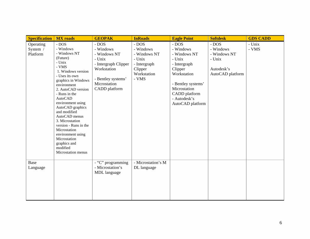
Specification MX roads GEOPAK InRoads Eagle Point Softdesk GDS CADD Operating System / Platform

- DOS - Windows - Windows NT (Future) - Unix - VMS 1. Windows version - Uses its own graphics in Windows environment 2. AutoCAD version - Runs in the AutoCAD environment using AutoCAD graphics and modified AutoCAD menus 3. Microstation version - Runs in the Microstation environment using Microstation graphics and modified Microstation menus

- DOS - Windows - Windows NT - Unix - Intergraph Clipper Workstation - Bentley systems’ Microstation CADD platform

- DOS - Windows - Windows NT - Unix - Intergraph Clipper Workstation - VMS

- DOS - Windows - Windows NT - Unix - Intergraph Clipper Workstation - Bentley systems’ Microstation CADD platform - Autodesk’s AutoCAD platform

- DOS - Windows - Windows NT - Unix Autodesk’s AutoCAD platform

- Unix - VMS

Base Language

- “C” programming - Microstation’s MDL language

- Microstation’s M DL language

7

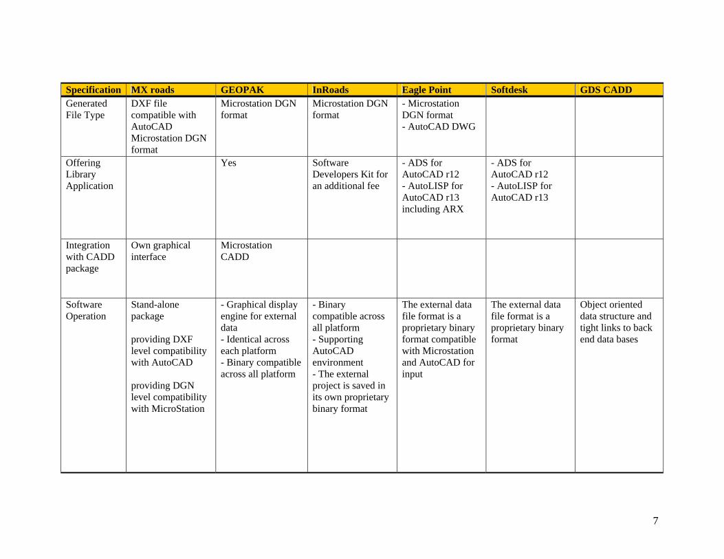
Specification MX roads GEOPAK InRoads Eagle Point Softdesk GDS CADD Generated File Type

DXF file compatible with AutoCAD Microstation DGN format

Microstation DGN format

Microstation DGN format

- Microstation DGN format - AutoCAD DWG

Offering Library Application

Yes Software Developers Kit for an additional fee

- ADS for AutoCAD r12 - AutoLISP for AutoCAD r13 including ARX

- ADS for AutoCAD r12 - AutoLISP for AutoCAD r13

Integration with CADD package

Own graphical interface

Microstation CADD

Software Operation

Stand-alone package providing DXF level compatibility with AutoCAD providing DGN level compatibility with MicroStation

- Graphical display engine for external data - Identical across each platform - Binary compatible across all platform

- Binary compatible across all platform - Supporting AutoCAD environment - The external project is saved in its own proprietary binary format

The external data file format is a proprietary binary format compatible with Microstation and AutoCAD for input

The external data file format is a proprietary binary format

Object oriented data structure and tight links to back end data bases

8

Specification MX roads GEOPAK InRoads Eagle Point Softdesk GDS CADD Strengthens - Internationally

recognized - Using 3D data “strings” to model surface features

- Comprehensiveness - Fully exploit the Microstation’s interactive - Flexibility - Easiness for use of graphic interface - Utilizing MDL - Change the geometry of the graphics and update or produce the external data

- Fully exploit the Microstation’s interactive - Flexibility - Easiness for use of graphic interface - Change the geometry of the graphics and update or produce the external data

Change the geometry of the graphics and update or produce the external data

Change the geometry of the graphics and update or produce the external data

Weakness

Slow acceptance of PC based CADD and AutoCAD in general in the public sector

9

Specification MX roads GEOPAK InRoads Eagle Point Softdesk GDS CADD Cost $5,500 with a $975

annual maintenance for Mxroad MAX including MX ROAD/MX RENEW/ MX DRAW $ 1500 for 1 student for full day $5000 for 6 to 8 engineers The commercial version includes the Windows environment and a choice of CAD environments. For an additional $750, both CAD environments are supplied with the commercial version.

$6,525 $6,000 $6,000 Maintenance per month is $100 Free upgrades On-site training at $165 per hour.

$5,000 for one seat of software. Training cost is $1195.00 per person Maintenance: Bronze Level: $2250.00 per year per seat, no limit to the number of modules you have. Silver Level: $1960.00 per year, per seat. Must have 50 modules or more for this level. Gold Level: $2450.00 per year, per seat. Must have 50 modules or more for this level.

3D data to model surface features

“Strings”

10

Table 2.2. Legend for Table 2.1 Acronym Definition ADS AutoCAD Development System

ARX ARX

AutoLISP AutoLISP is the scripting language for AutoCAD by Autodesk, a very crippled dynamic Lisp-1, based on very early xlisp

sources (v1.0), posted by David Betz on usenet (alt.sources), and without proper copyright laws that time used by Autodesk as their free scripting language.

CADD Computer Aided Drafting and Design

DGN Design

DWG AutoCAD File (File extension)

DXF AutoCAD File (file extension)

GDS Graphic Design Software

MDL MicroStation Development Language (C-like programming language for MicroStation)

VMS The official name of VMS is currently OpenVMS. VMS is a product of Compaq (after Compaq bougth Digital). VMS currently supports two hardware platforms: VAX and Alpha, and the variants are known as VMS VAX and VMS Alpha (or OpenVMS VAX and OpenVMS Alpha).

11

CHAPTER 3 Laser Scanning

3.1 Introduction

Laser scanning is a new technology that enables users to collect accurate geometrical as-

built data to be used later on for all kinds of applications, from military and space to

movie and entertainment. When activated, a laser scanner would send hundreds of laser

beams per second towards a user-specified object and retrieve these beams back, thus

measure the 3D position of each single point hit by each beam in the laser scanner’s

arbitrary local coordinate system with millimeter accuracy. All these positions are saved

in fully digital environment. This technology has several advantages, such as the ability

to capture detailed as-built description of objects out of reach and in short times.

In this pilot project, two companies were subcontracted to laser scan Bridgeport bridge

and Six Point bridge. Namely, Toronto-based Optech Incorporated1 and Indiana-based

Falk PLI2. On May 27, 2002 Optech carried out the laser scans of both bridges using

ILRIS-3D laser scanner. On the other hand, Falk PLI carried out the laser scan of

Bridgeport bridge on September 26, 2002 using Cyrax 25003 laser scanner, while rain

prevented the scan of Six Point bridge.

Although all point clouds can be exported into various CAD software packages like

AutoCAD, the huge amount of points (i.e. millions) could not be handled in these

packages. For the sake of processing the point clouds collected both by ILRIS-3D and

Cyrax 2500 laser scanners, the choice was made to use a software package called

Cyclone. Basically, it’s the same software used along with various types of Cyrax laser

scanners in the field.

1 http://www.optech.on.ca 2 http://www.falk-pli.com 3 http://www.cyra.com

12

3.2 Optech Survey

Bridgeport bridge was scanned before noon on May 27, 2002. It took twelve scans to

cover the whole bridge; five from east, five from west and two from the top of the bridge.

Six Point bridge was scanned in the afternoon, where it took ten scans to cover the whole

bridge; five from east, three from west and two from the top of the bridge, as seen in

Figure (3.1) below.

Figure 3.1: The scope of Optech’s twelve scans of Bridgeport bridge

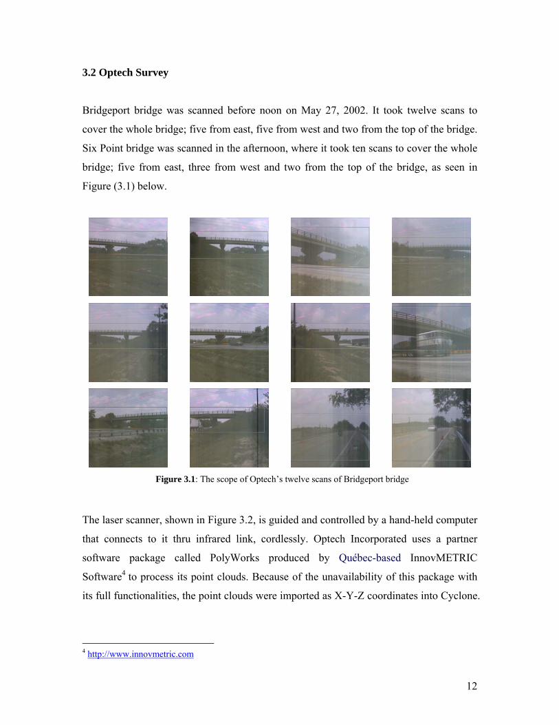
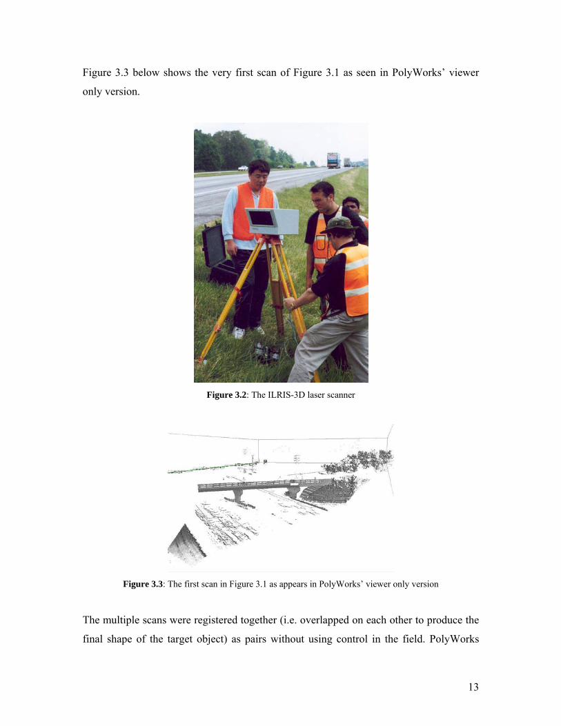
The laser scanner, shown in Figure 3.2, is guided and controlled by a hand-held computer

that connects to it thru infrared link, cordlessly. Optech Incorporated uses a partner

software package called PolyWorks produced by Québec-based InnovMETRIC

Software4 to process its point clouds. Because of the unavailability of this package with

its full functionalities, the point clouds were imported as X-Y-Z coordinates into Cyclone.

4 http://www.innovmetric.com

13

Figure 3.3 below shows the very first scan of Figure 3.1 as seen in PolyWorks’ viewer

only version.

Figure 3.2: The ILRIS-3D laser scanner

Figure 3.3: The first scan in Figure 3.1 as appears in PolyWorks’ viewer only version

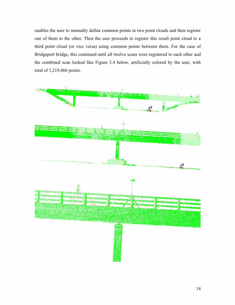
The multiple scans were registered together (i.e. overlapped on each other to produce the

final shape of the target object) as pairs without using control in the field. PolyWorks

14

enables the user to manually define common points in two point clouds and then register

one of them to the other. Then the user proceeds to register this result point cloud to a

third point cloud (or vice versa) using common points between them. For the case of

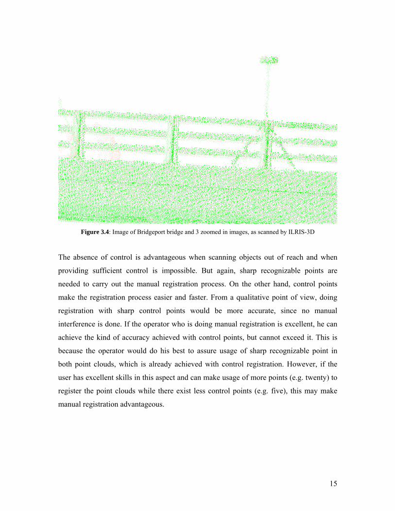
Bridgeport bridge, this continued until all twelve scans were registered to each other and

the combined scan looked like Figure 3.4 below, artificially colored by the user, with

total of 1,219,466 points.

15

Figure 3.4: Image of Bridgeport bridge and 3 zoomed in images, as scanned by ILRIS-3D

The absence of control is advantageous when scanning objects out of reach and when

providing sufficient control is impossible. But again, sharp recognizable points are

needed to carry out the manual registration process. On the other hand, control points

make the registration process easier and faster. From a qualitative point of view, doing

registration with sharp control points would be more accurate, since no manual

interference is done. If the operator who is doing manual registration is excellent, he can

achieve the kind of accuracy achieved with control points, but cannot exceed it. This is

because the operator would do his best to assure usage of sharp recognizable point in

both point clouds, which is already achieved with control registration. However, if the

user has excellent skills in this aspect and can make usage of more points (e.g. twenty) to

register the point clouds while there exist less control points (e.g. five), this may make

manual registration advantageous.

16

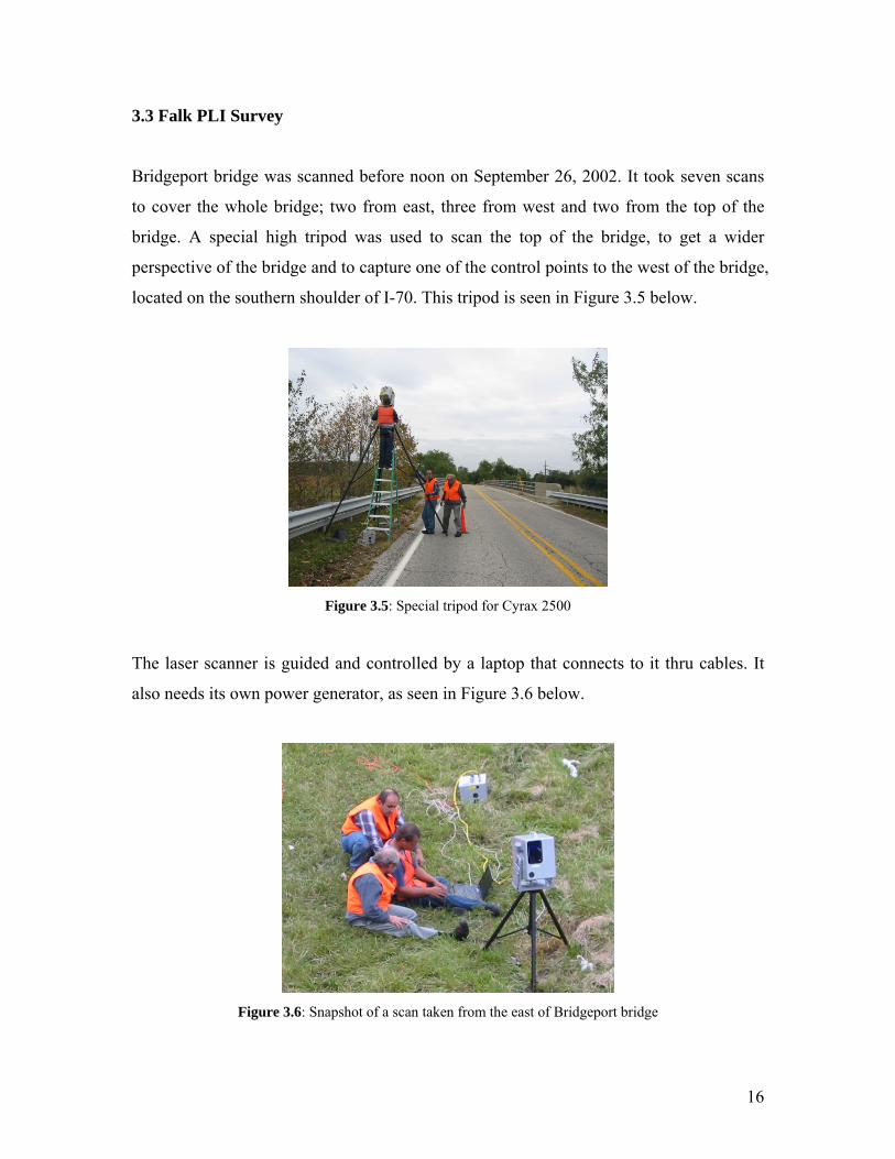
3.3 Falk PLI Survey

Bridgeport bridge was scanned before noon on September 26, 2002. It took seven scans

to cover the whole bridge; two from east, three from west and two from the top of the

bridge. A special high tripod was used to scan the top of the bridge, to get a wider

perspective of the bridge and to capture one of the control points to the west of the bridge,

located on the southern shoulder of I-70. This tripod is seen in Figure 3.5 below.

Figure 3.5: Special tripod for Cyrax 2500

The laser scanner is guided and controlled by a laptop that connects to it thru cables. It

also needs its own power generator, as seen in Figure 3.6 below.

Figure 3.6: Snapshot of a scan taken from the east of Bridgeport bridge

17

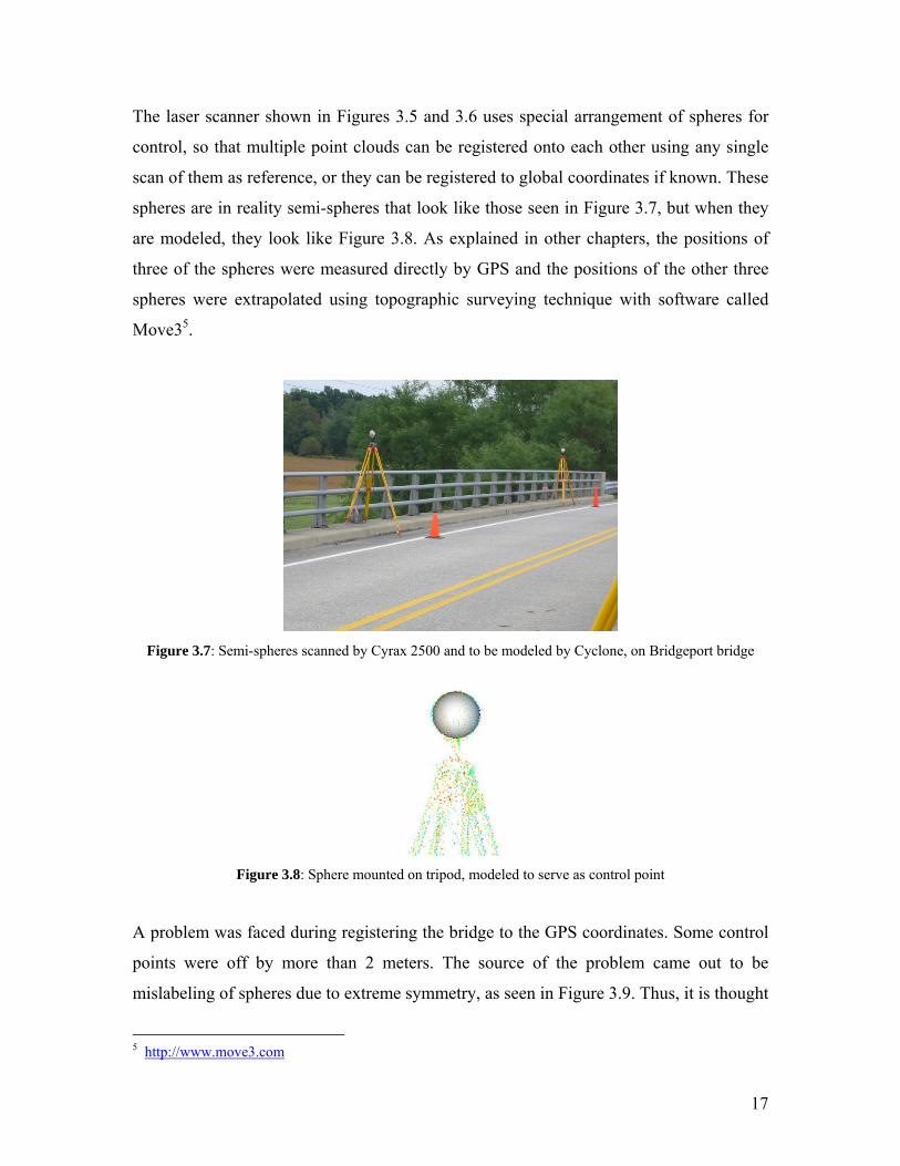
The laser scanner shown in Figures 3.5 and 3.6 uses special arrangement of spheres for

control, so that multiple point clouds can be registered onto each other using any single

scan of them as reference, or they can be registered to global coordinates if known. These

spheres are in reality semi-spheres that look like those seen in Figure 3.7, but when they

are modeled, they look like Figure 3.8. As explained in other chapters, the positions of

three of the spheres were measured directly by GPS and the positions of the other three

spheres were extrapolated using topographic surveying technique with software called

Move35.

Figure 3.7: Semi-spheres scanned by Cyrax 2500 and to be modeled by Cyclone, on Bridgeport bridge

Figure 3.8: Sphere mounted on tripod, modeled to serve as control point

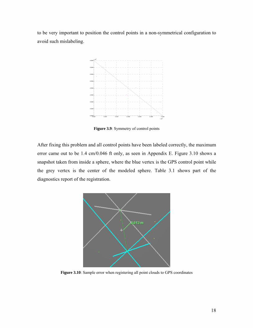
A problem was faced during registering the bridge to the GPS coordinates. Some control

points were off by more than 2 meters. The source of the problem came out to be

mislabeling of spheres due to extreme symmetry, as seen in Figure 3.9. Thus, it is thought

5 http://www.move3.com

18

to be very important to position the control points in a non-symmetrical configuration to

avoid such mislabeling.

3.1557 3.1557 3.1557 3.1558 3.1559 3.1559 3.1559

x 105

-4.9048

-4.9048

-4.9048

-4.9048

-4.9048

-4.9048

-4.9048

-4.9048

-4.9048x 106

Figure 3.9: Symmetry of control points

After fixing this problem and all control points have been labeled correctly, the maximum

error came out to be 1.4 cm/0.046 ft only, as seen in Appendix E. Figure 3.10 shows a

snapshot taken from inside a sphere, where the blue vertex is the GPS control point while

the grey vertex is the center of the modeled sphere. Table 3.1 shows part of the

diagnostics report of the registration.

Figure 3.10: Sample error when registering all point clouds to GPS coordinates

19

Table 3.1: Part of registration diagnostics report

Point’s ID Point Cloud to be Registered

Control Point Cloud

Type of Objects Registered

Error (m)

Error Vector (m)

S5 ScanWorld 6 FINAL_c6pts Sphere-Vertex 0.006 (0.004, 0.003, 0.001) S6 ScanWorld 6 FINAL_c6pts Sphere-Vertex 0.009 (0.008, 0.002, -0.003) S4 ScanWorld 6 FINAL_c6pts Sphere-Vertex 0.007 (0.000, -0.001, 0.007) S2 ScanWorld 6 FINAL_c6pts Sphere-Vertex 0.007 (-0.002, -0.005, 0.004) S3 ScanWorld 6 FINAL_c6pts Sphere-Vertex 0.014 (-0.005, 0.004, -0.013) S1 ScanWorld 6 FINAL_c6pts Sphere-Vertex 0.006 (-0.005, -0.002, 0.000) S2 ScanWorld 7 FINAL_c6pts Sphere-Vertex 0.006 (-0.002, -0.005, 0.002) S1 ScanWorld 7 FINAL_c6pts Sphere-Vertex 0.004 (-0.004, -0.001, 0.002)

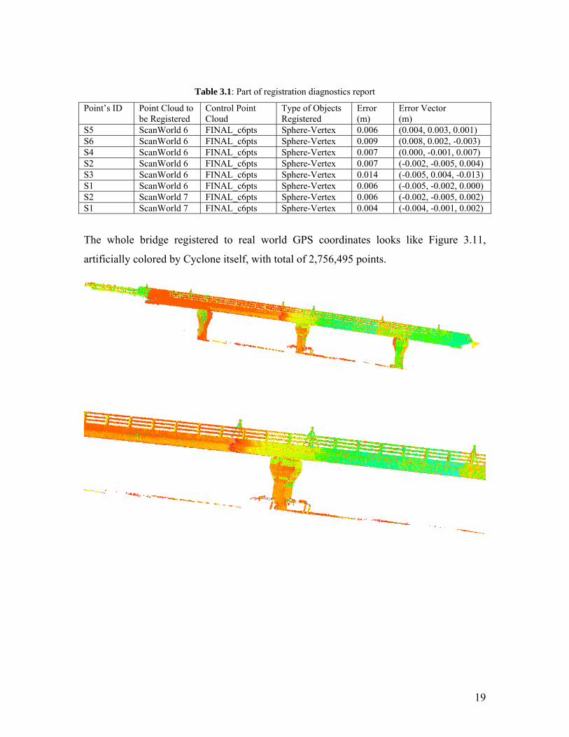
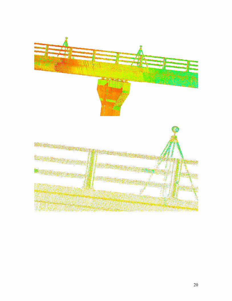
The whole bridge registered to real world GPS coordinates looks like Figure 3.11,

artificially colored by Cyclone itself, with total of 2,756,495 points.

20

21

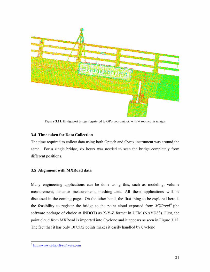
Figure 3.11: Bridgeport bridge registered to GPS coordinates, with 4 zoomed in images

3.4 Time taken for Data Collection

The time required to collect data using both Optech and Cyrax instrument was around the

same. For a single bridge, six hours was needed to scan the bridge completely from

different positions.

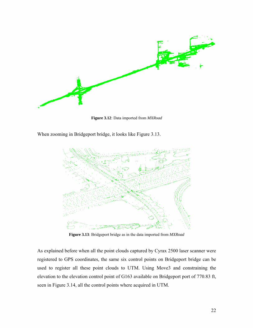
3.5 Alignment with MXRoad data

Many engineering applications can be done using this, such as modeling, volume

measurement, distance measurement, meshing…etc. All these applications will be

discussed in the coming pages. On the other hand, the first thing to be explored here is

the feasibility to register the bridge to the point cloud exported from MXRoad6 (the

software package of choice at INDOT) as X-Y-Z format in UTM (NAVD83). First, the

point cloud from MXRoad is imported into Cyclone and it appears as seen in Figure 3.12.

The fact that it has only 107,532 points makes it easily handled by Cyclone

6 http://www.cadapult-software.com

22

Figure 3.12: Data imported from MXRoad

When zooming in Bridgeport bridge, it looks like Figure 3.13.

Figure 3.13: Bridgeport bridge as in the data imported from MXRoad

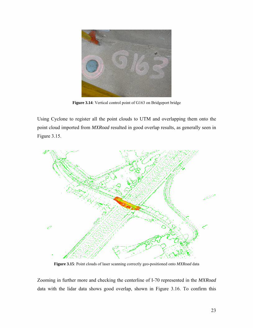
As explained before when all the point clouds captured by Cyrax 2500 laser scanner were

registered to GPS coordinates, the same six control points on Bridgeport bridge can be

used to register all these point clouds to UTM. Using Move3 and constraining the

elevation to the elevation control point of G163 available on Bridgeport port of 770.83 ft,

seen in Figure 3.14, all the control points where acquired in UTM.

23

Figure 3.14: Vertical control point of G163 on Bridgeport bridge

Using Cyclone to register all the point clouds to UTM and overlapping them onto the

point cloud imported from MXRoad resulted in good overlap results, as generally seen in

Figure 3.15.

Figure 3.15: Point clouds of laser scanning correctly geo-positioned onto MXRoad data

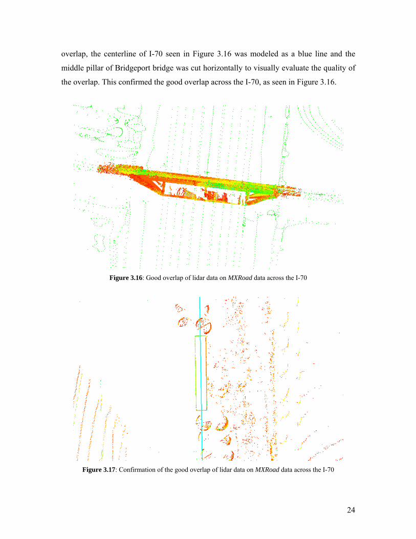
Zooming in further more and checking the centerline of I-70 represented in the MXRoad

data with the lidar data shows good overlap, shown in Figure 3.16. To confirm this

24

overlap, the centerline of I-70 seen in Figure 3.16 was modeled as a blue line and the

middle pillar of Bridgeport bridge was cut horizontally to visually evaluate the quality of

the overlap. This confirmed the good overlap across the I-70, as seen in Figure 3.16.

Figure 3.16: Good overlap of lidar data on MXRoad data across the I-70

Figure 3.17: Confirmation of the good overlap of lidar data on MXRoad data across the I-70

25

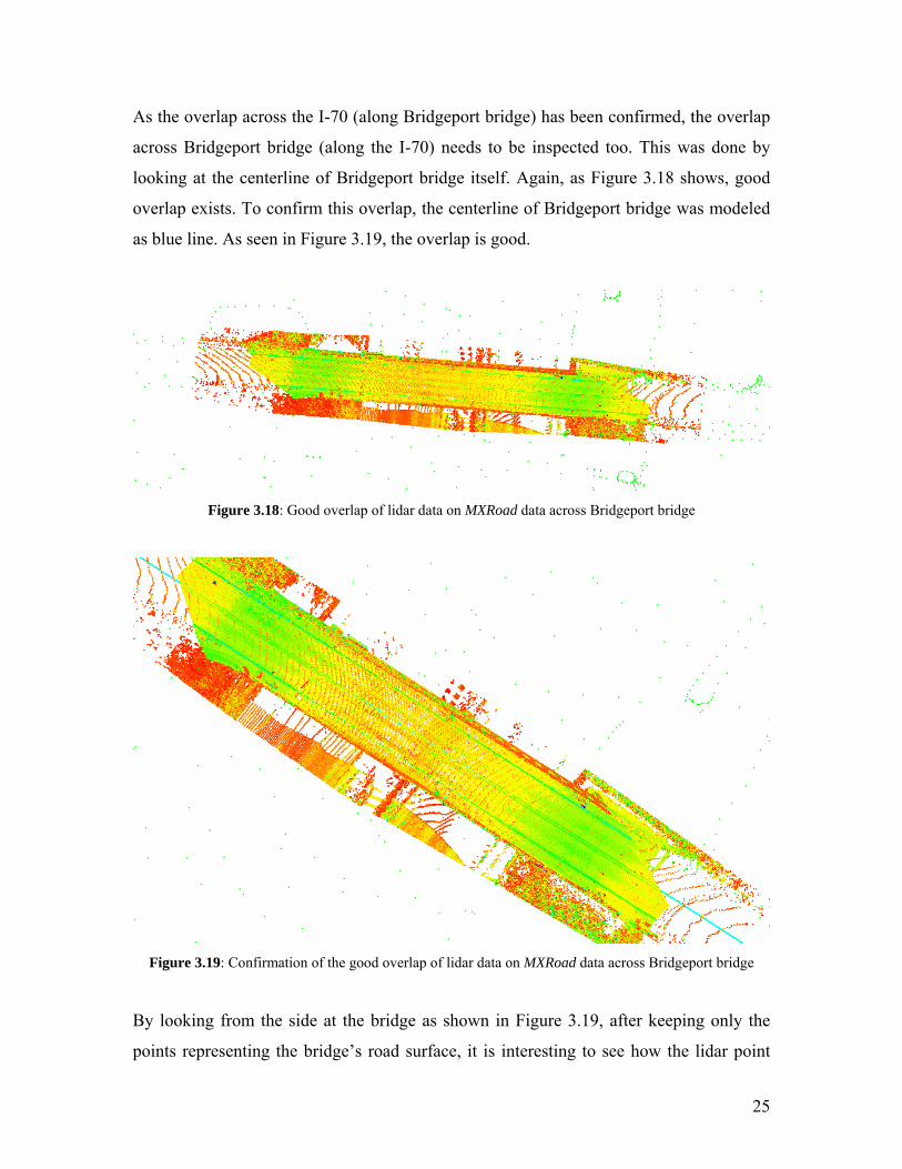
As the overlap across the I-70 (along Bridgeport bridge) has been confirmed, the overlap

across Bridgeport bridge (along the I-70) needs to be inspected too. This was done by

looking at the centerline of Bridgeport bridge itself. Again, as Figure 3.18 shows, good

overlap exists. To confirm this overlap, the centerline of Bridgeport bridge was modeled

as blue line. As seen in Figure 3.19, the overlap is good.

Figure 3.18: Good overlap of lidar data on MXRoad data across Bridgeport bridge

Figure 3.19: Confirmation of the good overlap of lidar data on MXRoad data across Bridgeport bridge

By looking from the side at the bridge as shown in Figure 3.19, after keeping only the

points representing the bridge’s road surface, it is interesting to see how the lidar point

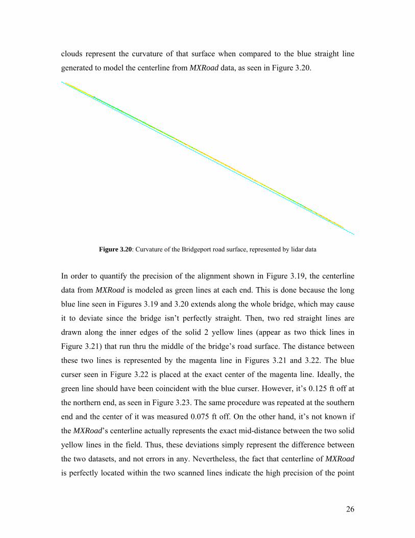
26

clouds represent the curvature of that surface when compared to the blue straight line

generated to model the centerline from MXRoad data, as seen in Figure 3.20.

Figure 3.20: Curvature of the Bridgeport road surface, represented by lidar data

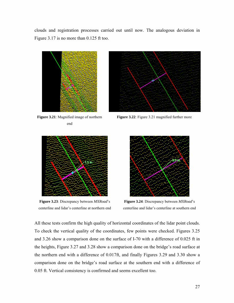
In order to quantify the precision of the alignment shown in Figure 3.19, the centerline

data from MXRoad is modeled as green lines at each end. This is done because the long

blue line seen in Figures 3.19 and 3.20 extends along the whole bridge, which may cause

it to deviate since the bridge isn’t perfectly straight. Then, two red straight lines are

drawn along the inner edges of the solid 2 yellow lines (appear as two thick lines in

Figure 3.21) that run thru the middle of the bridge’s road surface. The distance between

these two lines is represented by the magenta line in Figures 3.21 and 3.22. The blue

curser seen in Figure 3.22 is placed at the exact center of the magenta line. Ideally, the

green line should have been coincident with the blue curser. However, it’s 0.125 ft off at

the northern end, as seen in Figure 3.23. The same procedure was repeated at the southern

end and the center of it was measured 0.075 ft off. On the other hand, it’s not known if

the MXRoad’s centerline actually represents the exact mid-distance between the two solid

yellow lines in the field. Thus, these deviations simply represent the difference between

the two datasets, and not errors in any. Nevertheless, the fact that centerline of MXRoad

is perfectly located within the two scanned lines indicate the high precision of the point

27

clouds and registration processes carried out until now. The analogous deviation in

Figure 3.17 is no more than 0.125 ft too.

Figure 3.21: Magnified image of northern

end Figure 3.22: Figure 3.21 magnified further more

Figure 3.23: Discrepancy between MXRoad’s

centerline and lidar’s centerline at northern end Figure 3.24: Discrepancy between MXRoad’s

centerline and lidar’s centerline at southern end

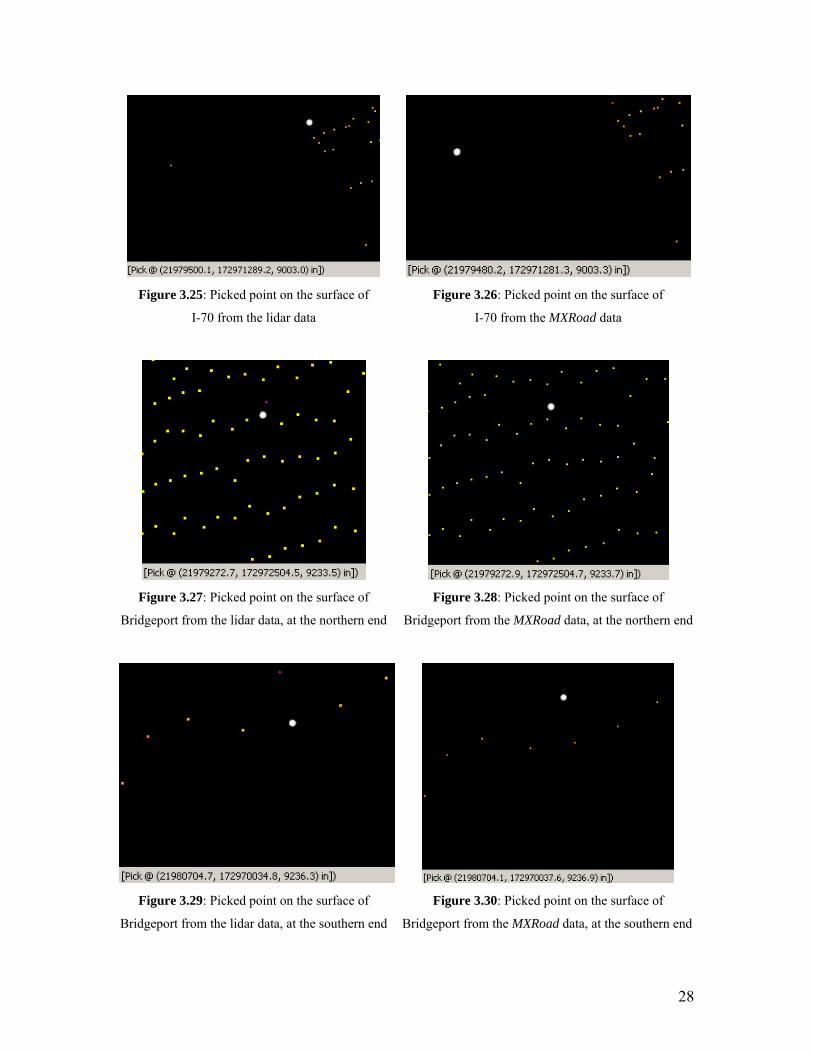
All these tests confirm the high quality of horizontal coordinates of the lidar point clouds.

To check the vertical quality of the coordinates, few points were checked. Figures 3.25

and 3.26 show a comparison done on the surface of I-70 with a difference of 0.025 ft in

the heights, Figure 3.27 and 3.28 show a comparison done on the bridge’s road surface at

the northern end with a difference of 0.017ft, and finally Figures 3.29 and 3.30 show a

comparison done on the bridge’s road surface at the southern end with a difference of

0.05 ft. Vertical consistency is confirmed and seems excellent too.

28

Figure 3.25: Picked point on the surface of

I-70 from the lidar data Figure 3.26: Picked point on the surface of

I-70 from the MXRoad data


Bridgeport from the lidar data, at the northern end Figure 3.28: Picked point on the surface of

Bridgeport from the MXRoad data, at the northern end


Bridgeport from the lidar data, at the southern end


Bridgeport from the MXRoad data, at the southern end

29

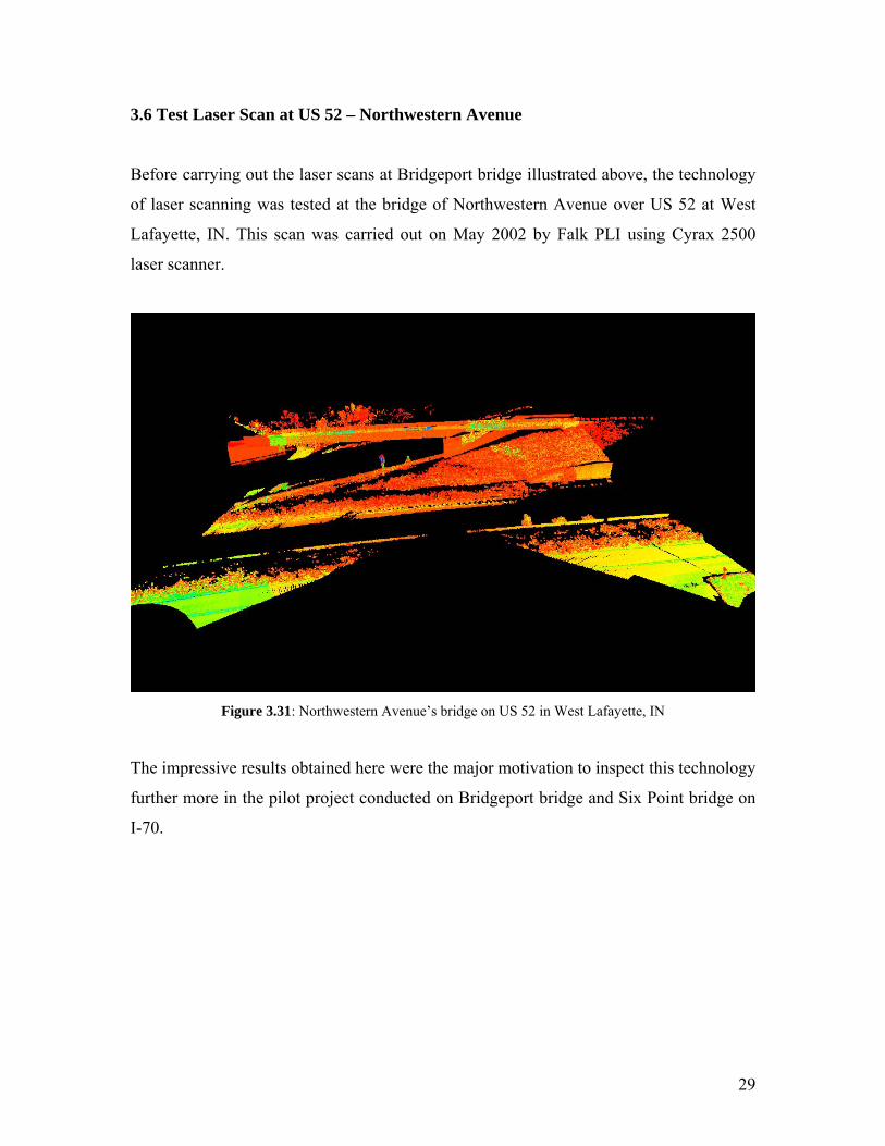
3.6 Test Laser Scan at US 52 – Northwestern Avenue

Before carrying out the laser scans at Bridgeport bridge illustrated above, the technology

of laser scanning was tested at the bridge of Northwestern Avenue over US 52 at West

Lafayette, IN. This scan was carried out on May 2002 by Falk PLI using Cyrax 2500

laser scanner.

Figure 3.31: Northwestern Avenue’s bridge on US 52 in West Lafayette, IN

The impressive results obtained here were the major motivation to inspect this technology

further more in the pilot project conducted on Bridgeport bridge and Six Point bridge on

I-70.

30

3.7 Engineering Applications

As mentioned before, various engineering applications can be done with such dense Lidar

point clouds like modeling, volume measurement, distance measurement, and meshing as

long as the software package is efficient in handling such huge volume of points.

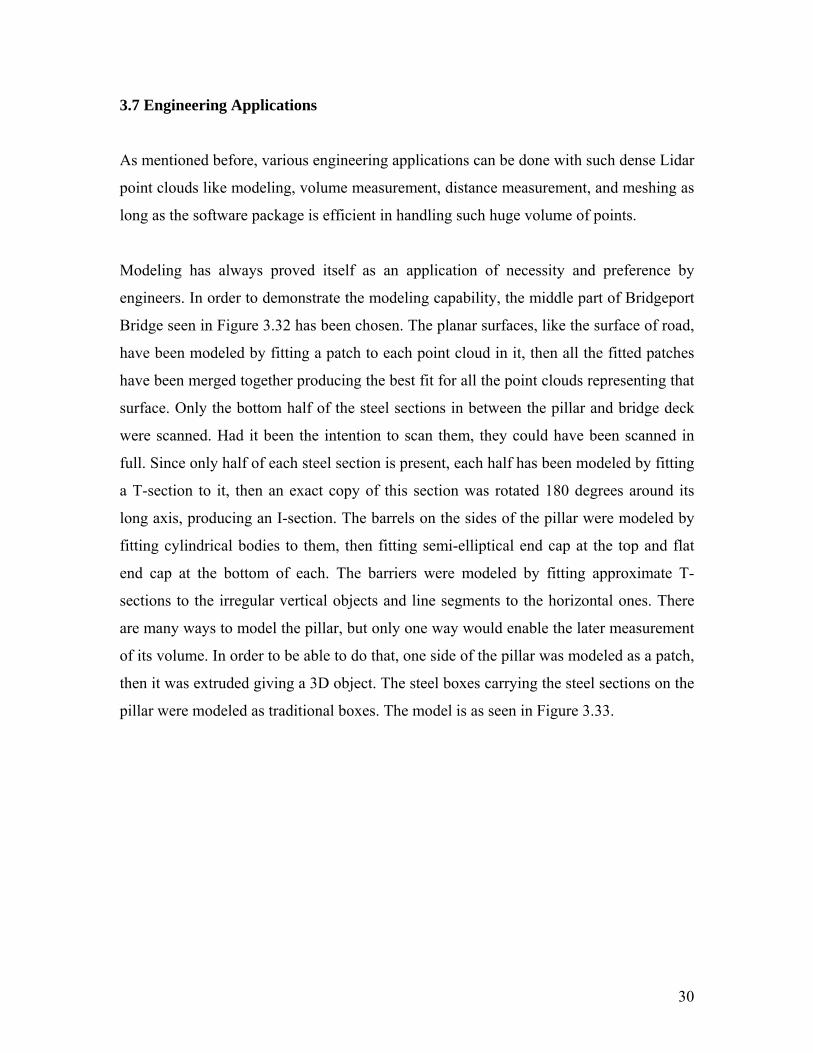
Modeling has always proved itself as an application of necessity and preference by

engineers. In order to demonstrate the modeling capability, the middle part of Bridgeport

Bridge seen in Figure 3.32 has been chosen. The planar surfaces, like the surface of road,

have been modeled by fitting a patch to each point cloud in it, then all the fitted patches

have been merged together producing the best fit for all the point clouds representing that

surface. Only the bottom half of the steel sections in between the pillar and bridge deck

were scanned. Had it been the intention to scan them, they could have been scanned in

full. Since only half of each steel section is present, each half has been modeled by fitting

a T-section to it, then an exact copy of this section was rotated 180 degrees around its

long axis, producing an I-section. The barrels on the sides of the pillar were modeled by

fitting cylindrical bodies to them, then fitting semi-elliptical end cap at the top and flat

end cap at the bottom of each. The barriers were modeled by fitting approximate T-

sections to the irregular vertical objects and line segments to the horizontal ones. There

are many ways to model the pillar, but only one way would enable the later measurement

of its volume. In order to be able to do that, one side of the pillar was modeled as a patch,

then it was extruded giving a 3D object. The steel boxes carrying the steel sections on the

pillar were modeled as traditional boxes. The model is as seen in Figure 3.33.

31

Figure 3.32: Mid-part of Bridgeport bridge, as point clouds represent it

Figure 3.33: Mid-part of Bridgeport bridge, after being modeled

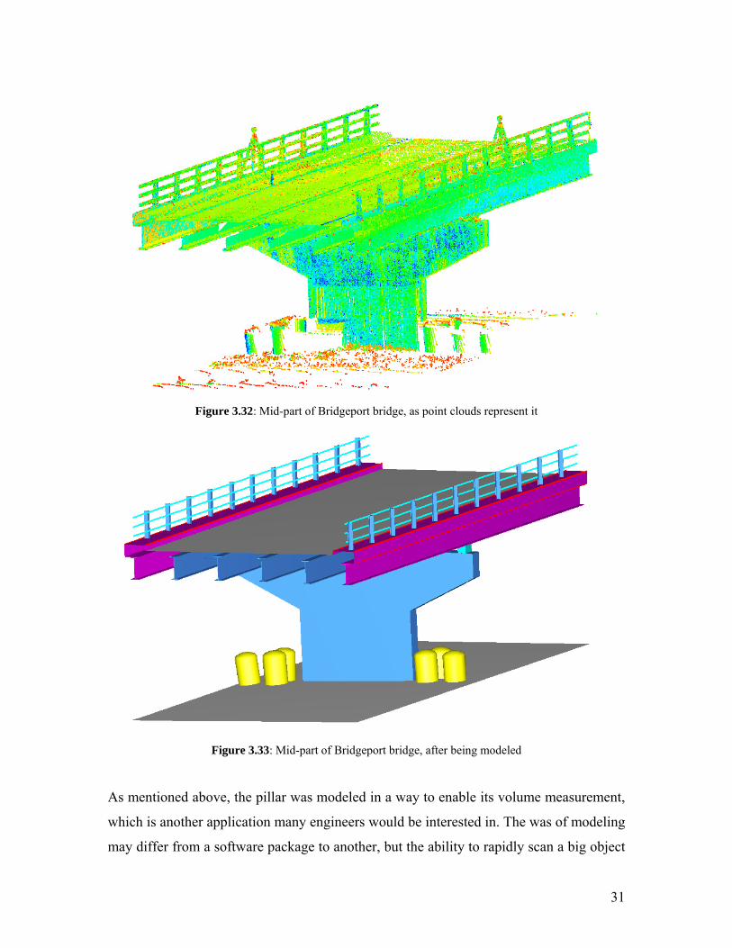
As mentioned above, the pillar was modeled in a way to enable its volume measurement,

which is another application many engineers would be interested in. The was of modeling

may differ from a software package to another, but the ability to rapidly scan a big object

32

in the field with challenging accessibility circumstances, and then measure its volume in

the comfort of office is certainly something engineers would like to have. Measuring the

volume of that pillar reveals 16.584 m3, which is equivalent to 585.668 ft3 as seen in

Figure 3.34.

Figure 3.34: The volume of modeled 3D bridge pillar

It should be noticed that the measured volume is as good as the model itself.

Also, engineers at the design stage would be very interested in knowing the amount of

soil to be removed to achieve a certain target within a certain area, or the amount of soil

above a certain reference plane that the design requires in that area. This task can be

easily achieved with laser scanning. The area under inspection should be scanned and the

point clouds belonging to any unnecessary objects can be removed. Then, the surface of

soil can be modeled using the meshing function, which doesn’t require regular or smooth

surfaces. After the soil is meshed, engineers can start assigning new reference planes to

achieve the volume of soil cut they are after. To apply these concepts on the case study in

hand, everything but the ground surface was removed. The ground surface in this case

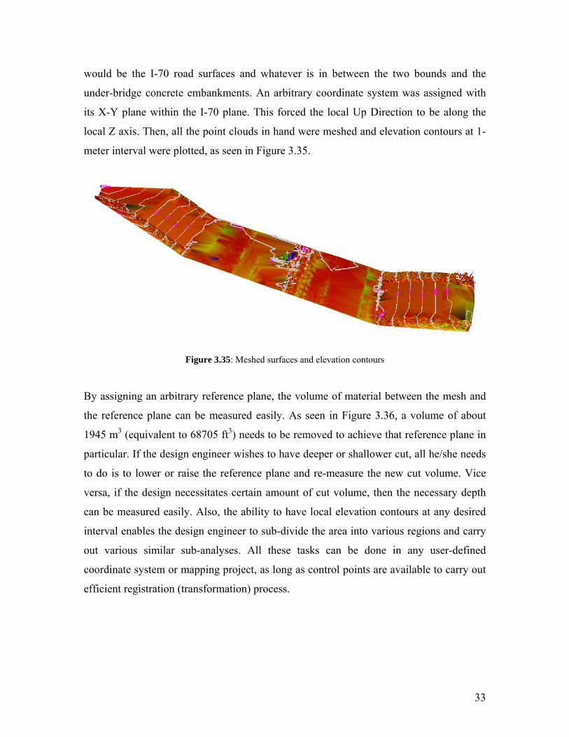
33

would be the I-70 road surfaces and whatever is in between the two bounds and the

under-bridge concrete embankments. An arbitrary coordinate system was assigned with

its X-Y plane within the I-70 plane. This forced the local Up Direction to be along the

local Z axis. Then, all the point clouds in hand were meshed and elevation contours at 1-

meter interval were plotted, as seen in Figure 3.35.

Figure 3.35: Meshed surfaces and elevation contours

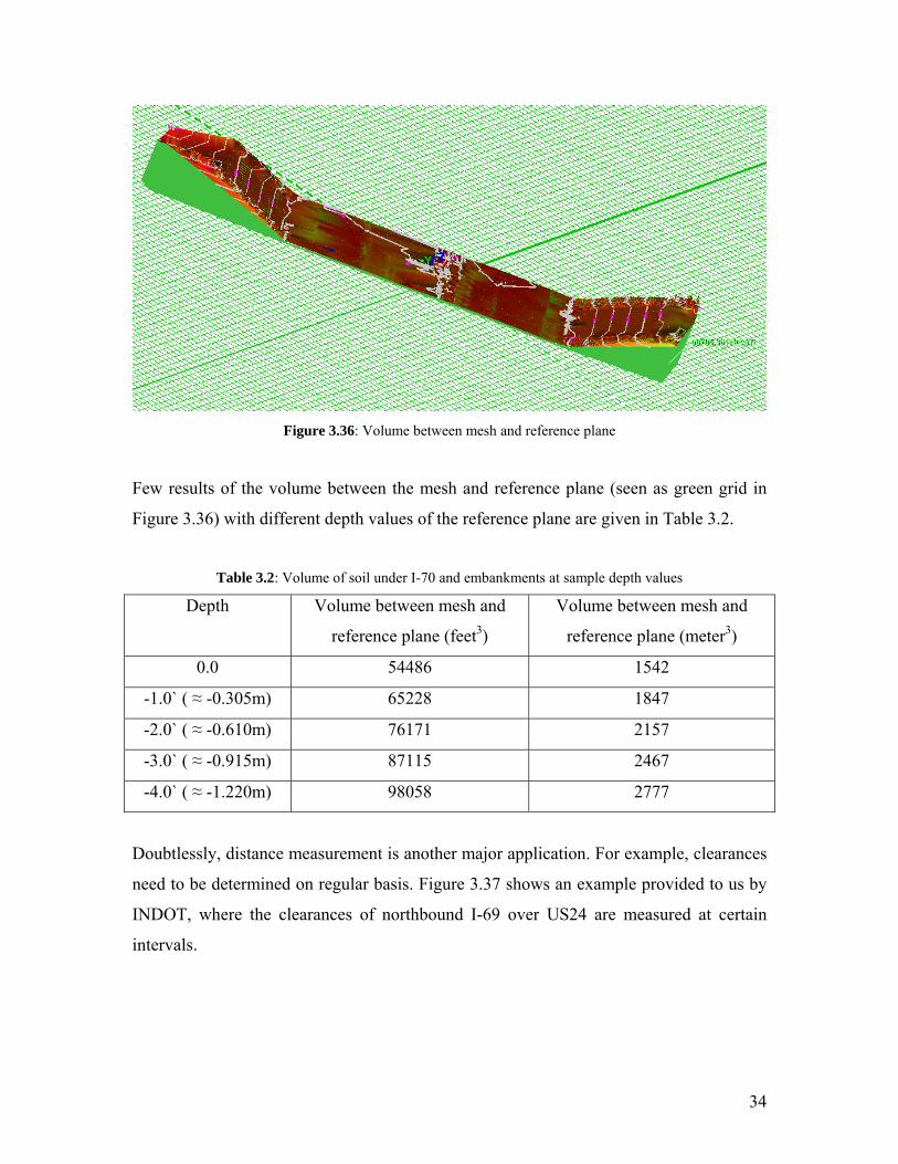
By assigning an arbitrary reference plane, the volume of material between the mesh and

the reference plane can be measured easily. As seen in Figure 3.36, a volume of about

1945 m3 (equivalent to 68705 ft3) needs to be removed to achieve that reference plane in

particular. If the design engineer wishes to have deeper or shallower cut, all he/she needs

to do is to lower or raise the reference plane and re-measure the new cut volume. Vice

versa, if the design necessitates certain amount of cut volume, then the necessary depth

can be measured easily. Also, the ability to have local elevation contours at any desired

interval enables the design engineer to sub-divide the area into various regions and carry

out various similar sub-analyses. All these tasks can be done in any user-defined

coordinate system or mapping project, as long as control points are available to carry out

efficient registration (transformation) process.

34

Figure 3.36: Volume between mesh and reference plane

Few results of the volume between the mesh and reference plane (seen as green grid in

Figure 3.36) with different depth values of the reference plane are given in Table 3.2.

Table 3.2: Volume of soil under I-70 and embankments at sample depth values

Depth Volume between mesh and

reference plane (feet3)

Volume between mesh and

reference plane (meter3)

0.0 54486 1542

-1.0` ( ≈ -0.305m) 65228 1847

-2.0` ( ≈ -0.610m) 76171 2157

-3.0` ( ≈ -0.915m) 87115 2467

-4.0` ( ≈ -1.220m) 98058 2777

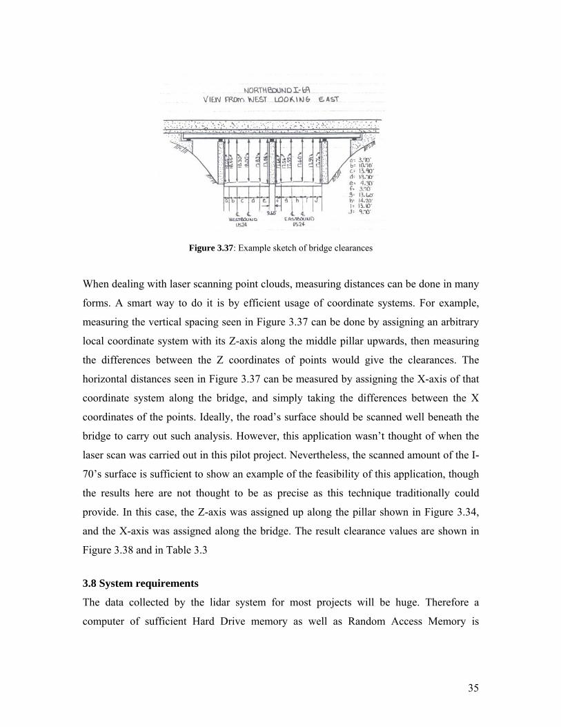
Doubtlessly, distance measurement is another major application. For example, clearances

need to be determined on regular basis. Figure 3.37 shows an example provided to us by

INDOT, where the clearances of northbound I-69 over US24 are measured at certain

intervals.

35

Figure 3.37: Example sketch of bridge clearances

When dealing with laser scanning point clouds, measuring distances can be done in many

forms. A smart way to do it is by efficient usage of coordinate systems. For example,

measuring the vertical spacing seen in Figure 3.37 can be done by assigning an arbitrary

local coordinate system with its Z-axis along the middle pillar upwards, then measuring

the differences between the Z coordinates of points would give the clearances. The

horizontal distances seen in Figure 3.37 can be measured by assigning the X-axis of that

coordinate system along the bridge, and simply taking the differences between the X

coordinates of the points. Ideally, the road’s surface should be scanned well beneath the

bridge to carry out such analysis. However, this application wasn’t thought of when the

laser scan was carried out in this pilot project. Nevertheless, the scanned amount of the I-

70’s surface is sufficient to show an example of the feasibility of this application, though

the results here are not thought to be as precise as this technique traditionally could

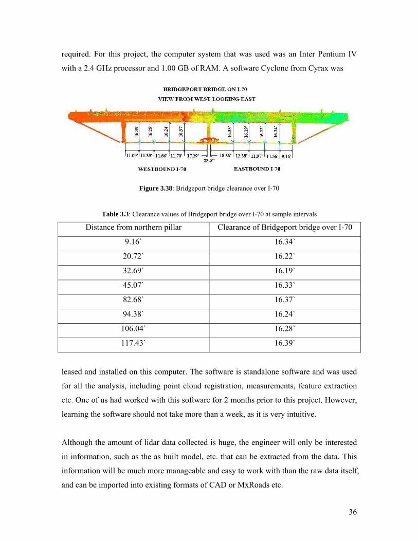
provide. In this case, the Z-axis was assigned up along the pillar shown in Figure 3.34,

and the X-axis was assigned along the bridge. The result clearance values are shown in

Figure 3.38 and in Table 3.3

3.8 System requirements

The data collected by the lidar system for most projects will be huge. Therefore a

computer of sufficient Hard Drive memory as well as Random Access Memory is

36

required. For this project, the computer system that was used was an Inter Pentium IV

with a 2.4 GHz processor and 1.00 GB of RAM. A software Cyclone from Cyrax was

Figure 3.38: Bridgeport bridge clearance over I-70

Table 3.3: Clearance values of Bridgeport bridge over I-70 at sample intervals Distance from northern pillar Clearance of Bridgeport bridge over I-70

9.16` 16.34`

20.72` 16.22`

32.69` 16.19`

45.07` 16.33`

82.68` 16.37`

94.38` 16.24`

106.04` 16.28`

117.43` 16.39`

leased and installed on this computer. The software is standalone software and was used

for all the analysis, including point cloud registration, measurements, feature extraction

etc. One of us had worked with this software for 2 months prior to this project. However,

learning the software should not take more than a week, as it is very intuitive.

Although the amount of lidar data collected is huge, the engineer will only be interested

in information, such as the as built model, etc. that can be extracted from the data. This

information will be much more manageable and easy to work with than the raw data itself,

and can be imported into existing formats of CAD or MxRoads etc.

37

CHAPTER 4 Satellite Imagery (QuickBird Image Rectification)

This chapter documents the generation of the rectified QuickBird satellite image of the project

area.

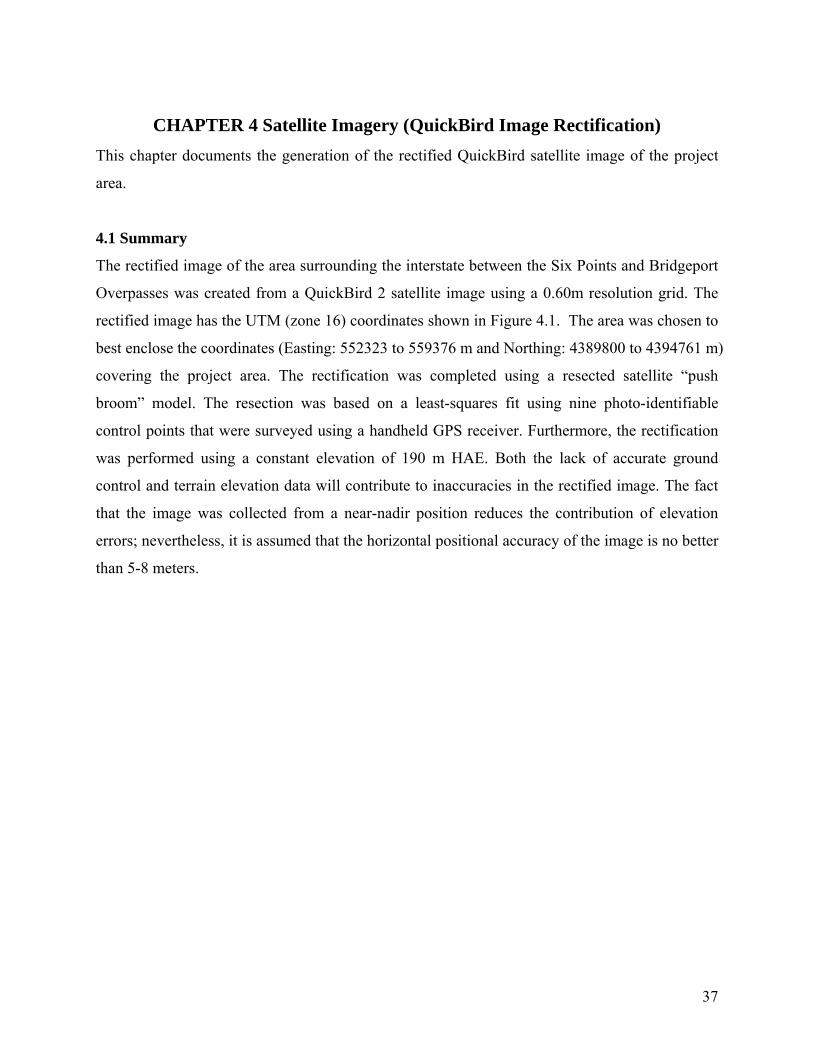
4.1 Summary

The rectified image of the area surrounding the interstate between the Six Points and Bridgeport

Overpasses was created from a QuickBird 2 satellite image using a 0.60m resolution grid. The

rectified image has the UTM (zone 16) coordinates shown in Figure 4.1. The area was chosen to

best enclose the coordinates (Easting: 552323 to 559376 m and Northing: 4389800 to 4394761 m)

covering the project area. The rectification was completed using a resected satellite “push

broom” model. The resection was based on a least-squares fit using nine photo-identifiable

control points that were surveyed using a handheld GPS receiver. Furthermore, the rectification

was performed using a constant elevation of 190 m HAE. Both the lack of accurate ground

control and terrain elevation data will contribute to inaccuracies in the rectified image. The fact

that the image was collected from a near-nadir position reduces the contribution of elevation

errors; nevertheless, it is assumed that the horizontal positional accuracy of the image is no better

than 5-8 meters.

38

Figure 4.1 Rectified Satellite Imagery

The following paragraphs provide additional details concerning the individual elements of image

rectification.

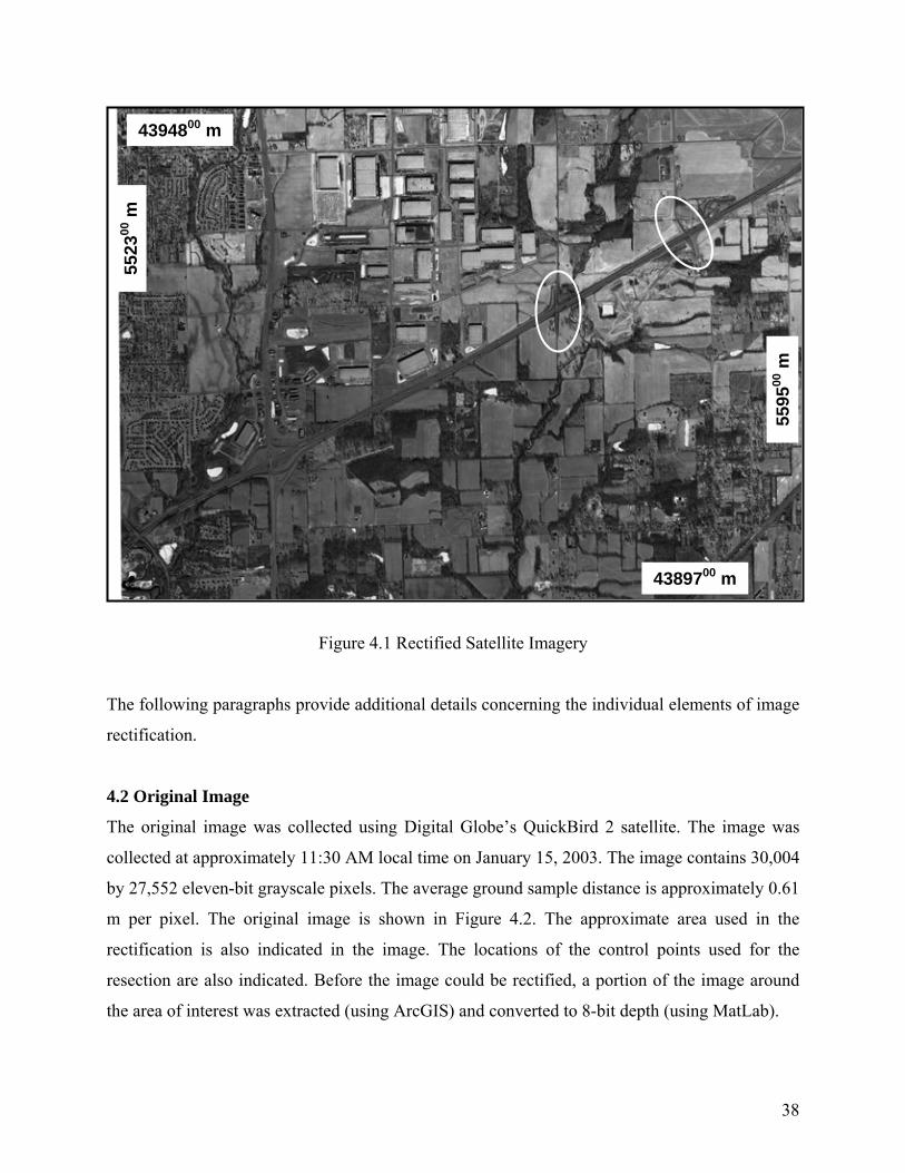
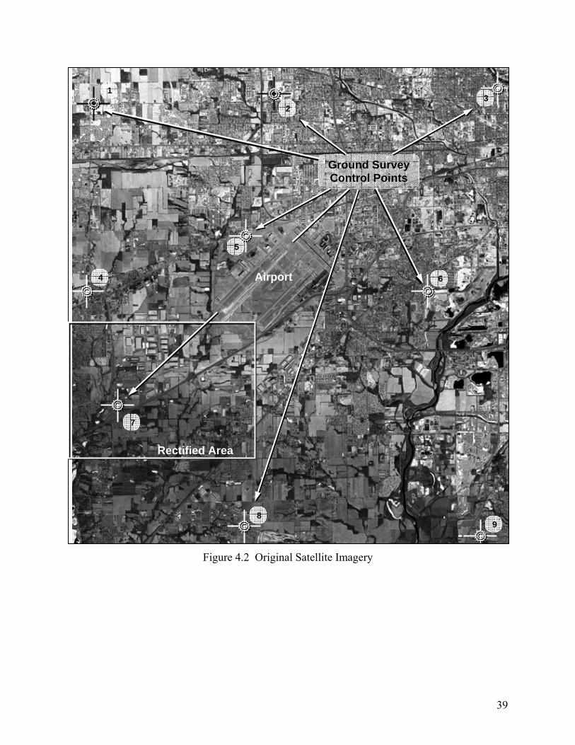
4.2 Original Image

The original image was collected using Digital Globe’s QuickBird 2 satellite. The image was

collected at approximately 11:30 AM local time on January 15, 2003. The image contains 30,004

by 27,552 eleven-bit grayscale pixels. The average ground sample distance is approximately 0.61

m per pixel. The original image is shown in Figure 4.2. The approximate area used in the

rectification is also indicated in the image. The locations of the control points used for the

resection are also indicated. Before the image could be rectified, a portion of the image around

the area of interest was extracted (using ArcGIS) and converted to 8-bit depth (using MatLab).

4394800 m

4389700 m

5523

00 m

5595

00 m

39

Figure 4.2 Original Satellite Imagery

1

23

4

5

6

7

89

Rectified Area

Ground Survey Control Points

Airport

40

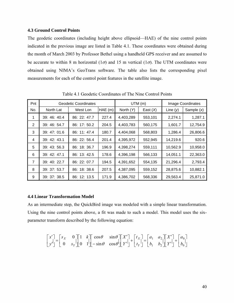
4.3 Ground Control Points

The geodetic coordinates (including height above ellipsoid—HAE) of the nine control points

indicated in the previous image are listed in Table 4.1. These coordinates were obtained during

the month of March 2003 by Professor Bethel using a handheld GPS receiver and are assumed to

be accurate to within 8 m horizontal (1σ) and 15 m vertical (1σ). The UTM coordinates were

obtained using NIMA’s GeoTrans software. The table also lists the corresponding pixel

measurements for each of the control point features in the satellite image.

Table 4.1 Geodetic Coordinates of The Nine Control Points

Pnt Geodetic Coordinates UTM (m) Image Coordinates No. North Lat West Lon HAE (m) North (Y) East (X) Line (y) Sample (x)

1 39: 46: 40.4 86: 22: 47.7 227.4 4,403,289 553,101 2,274.1 1,287.1

2 39: 46: 54.7 86: 17: 50.2 204.5 4,403,783 560,175 1,601.7 12,754.9

3 39: 47: 01.6 86: 11: 47.4 180.7 4,404,068 568,803 1,286.4 26,806.6

4 39: 42: 43.1 86: 22: 56.4 201.4 4,395,972 552,945 14,219.6 920.6

5 39: 43: 56.3 86: 18: 36.7 196.9 4,398,274 559,111 10,562.9 10,958.0

6 39: 42: 47.1 86: 13: 42.5 178.6 4,396,198 566,133 14,051.1 22,363.0

7 39: 40: 22.7 86: 22: 07.7 194.5 4,391,652 554,135 21,296.4 2,793.4

8 39: 37: 53.7 86: 18: 38.6 207.5 4,387,095 559,152 28,875.6 10,882.1

9 39: 37: 38.5 86: 12: 13.5 171.9 4,386,702 568,336 29,563.4 25,871.0

4.4 Linear Transformation Model

As an intermediate step, the QuickBird image was modeled with a simple linear transformation.

Using the nine control points above, a fit was made to such a model. This model uses the six-

parameter transform described by the following equation:

⎥⎦

⎤⎢⎣

⎡+⎥

⎦

⎤⎢⎣

⎡′′

⎥⎦

⎤⎢⎣

⎡=⎥

⎦

⎤⎢⎣

⎡+⎥

⎦

⎤⎢⎣

⎡′′

⎥⎦

⎤⎢⎣

⎡−⎥

⎦

⎤⎢⎣

⎡⎥⎦

⎤⎢⎣

⎡=⎥

⎦

⎤⎢⎣

⎡′′

0

0

21

21

cossinsincos

101

00

ba

YX

bbaa

tt

YXk

ss

yx

Y

X

Y

X

θθθθ

41

where (x', y') are the pre-shifted and scaled image coordinates and (X', Y') are the pre-shifted and

scaled UTM ground coordinates1. The model allows for an additional translation (tX and tY) and

scaling (sX and sY) of the X'- and Y'-axes, a rotation (θ) about the vertical, and a skewing (k) of

the axes to allow for non-orthogonality in the image. These six parameters were combined into

the six elements ai and bi as shown above. Only three control points would be needed to

completely define these six parameters. The redundancy provided by the nine control points

allowed for a least-squares fit. The computed values for these six composite elements are

indicated in the following table below with the pre-transformation shifts and scalings for the

coordinate systems. The resulting residual for each control point measurement is presented in

Table 4.2.

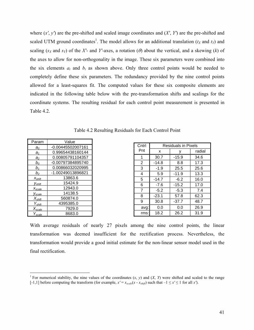
Table 4.2 Resulting Residuals for Each Control Point

1 For numerical stability, the nine values of the coordinates (x, y) and (X, Y) were shifted and scaled to the range [-1,1] before computing the transform (for example, x' = xscale(x - xshift) such that –1 ≤ x' ≤ 1 for all x').

Param Value a0 -0.00445502007161 a1 0.99654438160144 a2 0.00805791104357 b0 -0.00797384895740 b1 0.00866032020995 b2 -1.00249013896821

xshift 13863.6 yshift 15424.9 xscale 12943.0 yscale 14138.5 Xshift 560874.0 Yshift 4395385.0 Xscale 7929.0 Yscale 8683.0

Residuals in Pixels Cntrl

Pnt x y radial 1 30.7 -15.9 34.6 2 -14.8 8.8 17.3 3 -1.9 25.5 25.6 4 5.9 -11.9 13.3 5 -14.7 -6.2 16.0 6 -7.6 -15.2 17.0 7 -5.2 -5.3 7.4 8 -23.1 57.8 62.3 9 30.8 -37.7 48.7 avg: 0.0 0.0 26.9 rms: 18.2 26.2 31.9

With average residuals of nearly 27 pixels among the nine control points, the linear

transformation was deemed insufficient for the rectification process. Nevertheless, the

transformation would provide a good initial estimate for the non-linear sensor model used in the

final rectification.

42

4.5 Non-Linear Sensor Model

A non-linear orbital model for a “push broom” sensor was adopted to more correctly model the

QuickBird sensor. This model included six typical Keplerian orbit parameters: semi-major

axis—a, eccentricity—e, inclination—i, longitude of ascending node—Ω; argument of perigee—

ω, and time of image’s center line (relative to time at ascending node)—tf. It also included the

average time per line and optical principle distance. Finally, the model allowed for up to second-

order, time-varying adjustments in the sensor position (Cartesian coordinates relative to the

earth-centered-earth-fixed system: XECF, YECF, ZECF) and attitude (Euler angles; ω, φ, κ; about the

sensor’s principle axes; x, y, and z; respectively). These latter parameters were applied in the

following manner:

2

210 ΔtpΔtpppp ⋅+⋅++=′ δδδ

where p´ is an adjusted position or attitude value, p is an unadjusted position or attitude value,

δpi are the model’s adjustment parameters for the corresponding position or attitude values, and

Δt is the time offset from the collection time for the image’s center line.

4.6 Image Resection

Using the non-linear sensor model and ground control points described above, the original image

was resected, providing refined values for each of the model parameters. These resection values

are given in Table 4.3. These values were those used in the image rectification. The residuals for

the nine control point measurements using the refined model values are provided in the second

table. These residuals are approximately three times smaller than those obtained with the linear

model, and are well within the accuracy of the surveyed ground control points (approximately,

13 pixels 1σ).

43

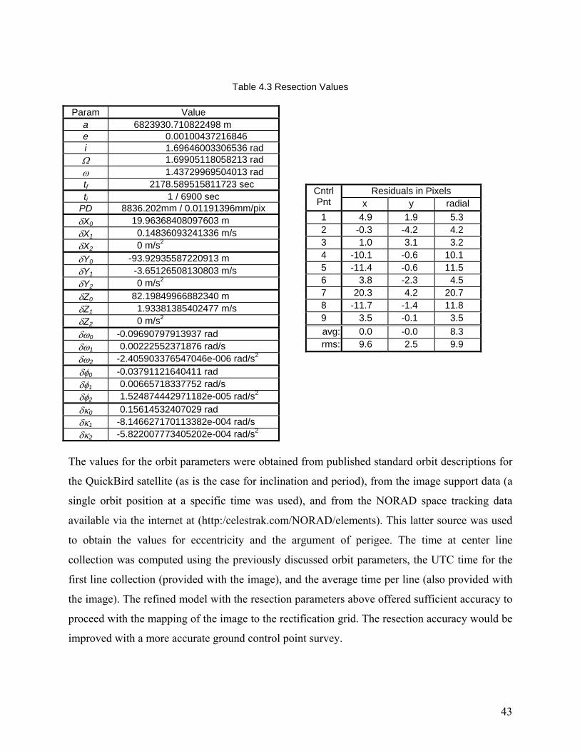
Table 4.3 Resection Values

Param Value

a 6823930.710822498 m e 0.00100437216846 i 1.69646003306536 rad

Ω 1.69905118058213 rad ω 1.43729969504013 rad tf 2178.589515811723 sec ti 1 / 6900 sec

PD 8836.202mm / 0.01191396mm/pix δX0 19.96368408097603 m δX1 0.14836093241336 m/s δX2 0 m/s2 δY0 -93.92935587220913 m δY1 -3.65126508130803 m/s δY2 0 m/s2 δZ0 82.19849966882340 m δZ1 1.93381385402477 m/s δZ2 0 m/s2 δω0 -0.09690797913937 rad δω1 0.00222552371876 rad/s δω2 -2.405903376547046e-006 rad/s2 δφ0 -0.03791121640411 rad δφ1 0.00665718337752 rad/s δφ2 1.524874442971182e-005 rad/s2 δκ0 0.15614532407029 rad δκ1 -8.146627170113382e-004 rad/s δκ2 -5.822007773405202e-004 rad/s2

Residuals in Pixels Cntrl Pnt x y radial 1 4.9 1.9 5.3 2 -0.3 -4.2 4.2 3 1.0 3.1 3.2 4 -10.1 -0.6 10.1 5 -11.4 -0.6 11.5 6 3.8 -2.3 4.5 7 20.3 4.2 20.7 8 -11.7 -1.4 11.8 9 3.5 -0.1 3.5 avg: 0.0 -0.0 8.3 rms: 9.6 2.5 9.9

The values for the orbit parameters were obtained from published standard orbit descriptions for

the QuickBird satellite (as is the case for inclination and period), from the image support data (a

single orbit position at a specific time was used), and from the NORAD space tracking data

available via the internet at (http:/celestrak.com/NORAD/elements). This latter source was used

to obtain the values for eccentricity and the argument of perigee. The time at center line

collection was computed using the previously discussed orbit parameters, the UTC time for the

first line collection (provided with the image), and the average time per line (also provided with

the image). The refined model with the resection parameters above offered sufficient accuracy to

proceed with the mapping of the image to the rectification grid. The resection accuracy would be

improved with a more accurate ground control point survey.

44

4.7 Rectification Grid

To have all the data used in the project be in the same coordinate system a UTM-coordinate grid

was established to capture the area of interest. This grid had a step size of 0.6 m in both the north

and east directions. The grid covered from 552,300 to 559,500 m in Easting and 4,389,700 to

4,394,800 m in Northing (UTM zone 16)— an area of 7.2 km by 5.1 km. This grid would result

in an image of 12000 by 8500 pixels.

4.8 Image Rectification

For an element of the rectification grid, the corresponding image coordinate had to be

determined using the refined non-linear sensor model. This calculation required an initial image

coordinate estimate (determined using the linear transformation discussed above). The

approximated image line could then be used to estimate the time of collection. Using the sensor

model, the gradient for the error surface near the estimate was determined. The two-dimensional

gradient was then used to solve for a final image coordinate (x, y) corresponding to the grid

element (X, Y). The gray-level value for the rectified grid pixel was then determined by

interpolating (a bilinear interpolation scheme was used) between the gray values for the nearest

four pixels in the original image. These steps were repeated for each of the 102 million pixels in

the rectification grid.

4.9 Potential Improvements

The following items are for consideration for future improvements upon the process outlined in

this chapter:

• A high accuracy survey of ground control points within the image. This should include points

distributed throughout the image (such as the existing points) and could include additional

points near the area of interest. All points must be recognizable and unambiguous in the

QuickBird image.

• Modification of the available TIFF tools to accept 16-bit images and to interpret GeoTIFF

tags.

• Modification of the sensor model to allow parameter adjustments along the orbit axes rather

than in the ECEF frame.

• Modification of the sensor model to use ephemeris data provided with the image.

45

• Allowance for rectification using the rational polynomial coefficients provided with the

image.

• Error propagation calculations for each of the above models.

46

CHAPTER 5 Control

To enable to put the lidar survey “on the map”, the three dimensional coordinates of a

sufficient number of well identifiable points in the (combined) Lidar point cloud had to

be determined. This absolute orientation, to use photogrammetric terminology, was

performed in a two step process. Section 5.1 describes how horizontal coordinates were

brought to the Bridgeport Bridge by a GPS survey via horizontal control as provided by

NGS control points in the vicinity of the project. A local survey using a total station

(section 5.2) completed the absolute orientation in horizontal and vertical sense.

Appendices C and D give more a more detailed background of the GPS survey and total

station survey, respectively.

5.1 Global Positioning System (GPS)

Introduction

GPS is a radio-navigation system developed by the Department of Defense. It is a

worldwide space-based system that consists of fully operational 24 satellites orbiting the

earth in six circular orbits at an altitude of 20200 km. As its name indicates, its major

function is to pinpoint 3D locations using specially manufactured receivers.

Because of the availability of many local, regional and global reference frames, the

decision has been made to use the GPS technology to get points on Bridgeport bridge and

Six Point bridge in its reference frame: World Geodetic System 1984 (WGS84). When

combined with classical topographic survey of several other points on both bridges, this

will make it possible to transform the bridges to other reference frames, like State Plane

Coordinate System.

47

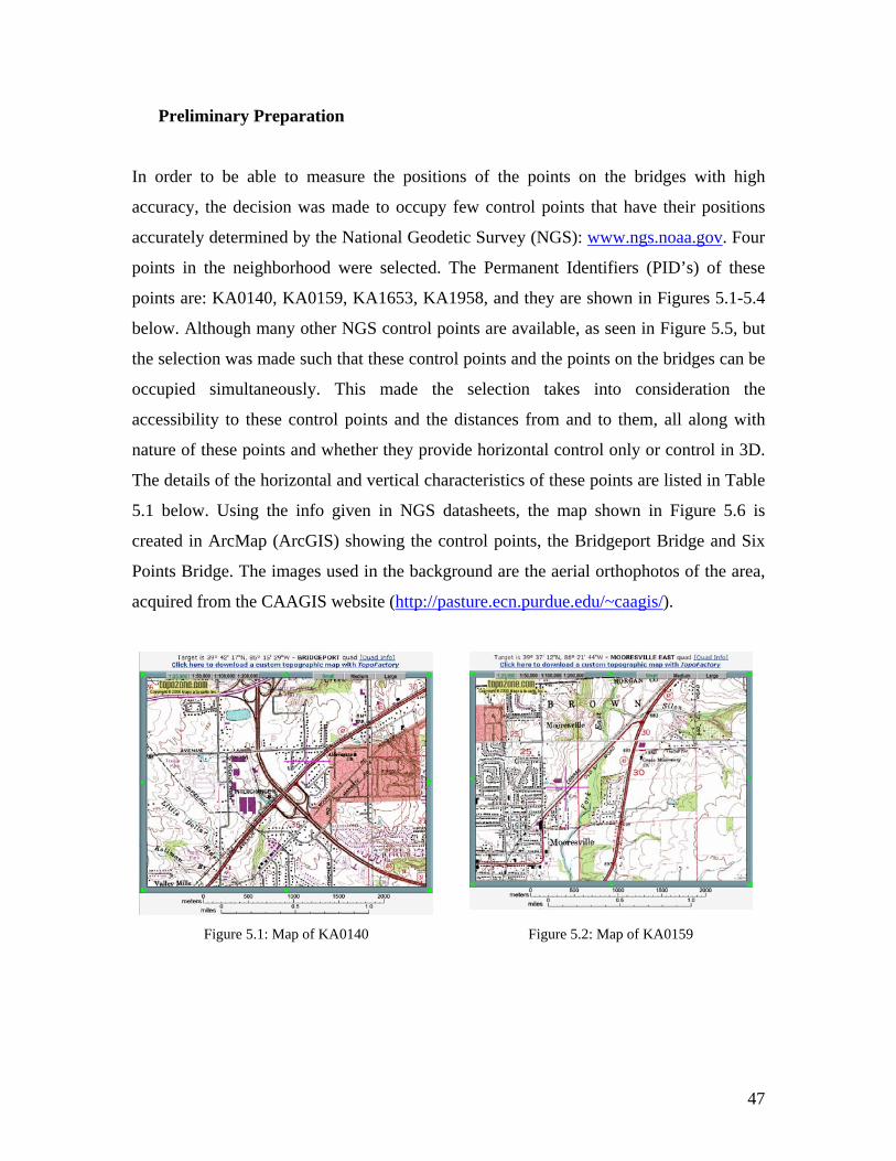
Preliminary Preparation

In order to be able to measure the positions of the points on the bridges with high

accuracy, the decision was made to occupy few control points that have their positions

accurately determined by the National Geodetic Survey (NGS): www.ngs.noaa.gov. Four

points in the neighborhood were selected. The Permanent Identifiers (PID’s) of these

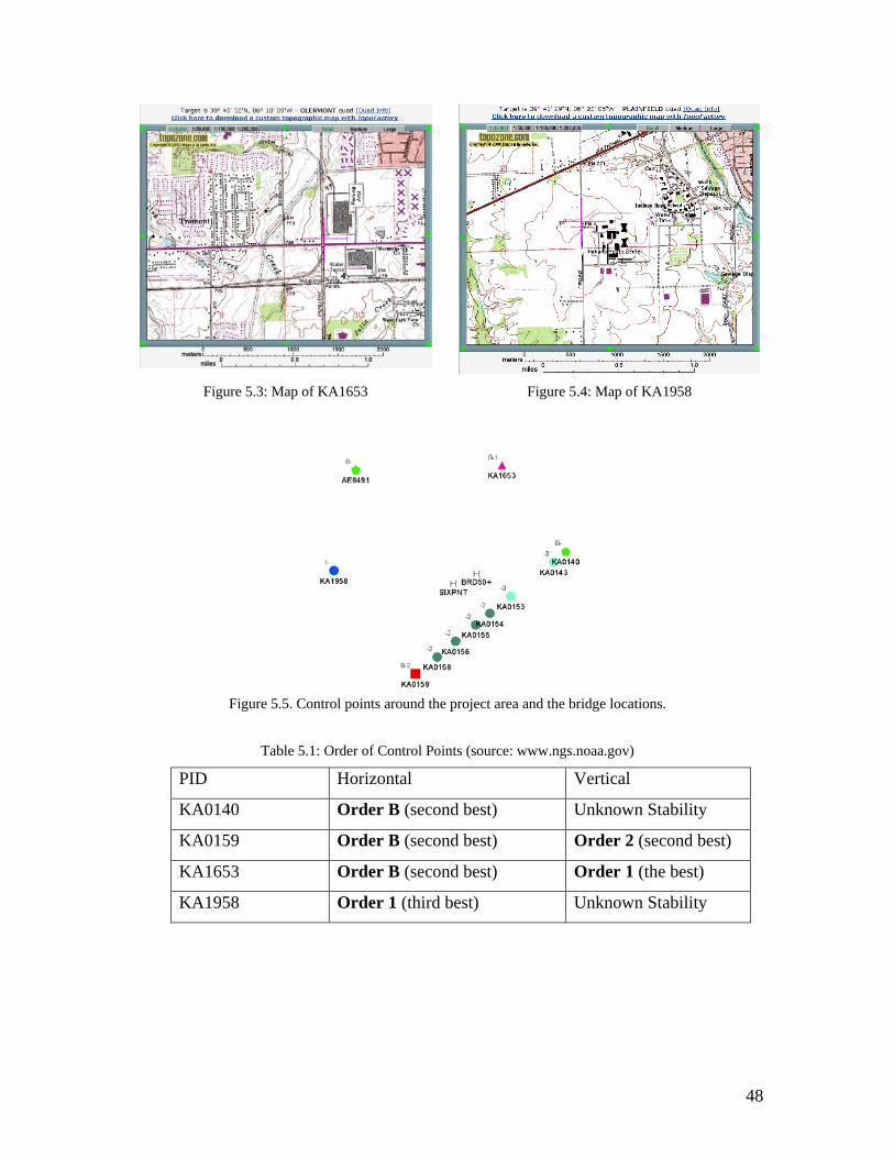
points are: KA0140, KA0159, KA1653, KA1958, and they are shown in Figures 5.1-5.4

below. Although many other NGS control points are available, as seen in Figure 5.5, but

the selection was made such that these control points and the points on the bridges can be

occupied simultaneously. This made the selection takes into consideration the

accessibility to these control points and the distances from and to them, all along with

nature of these points and whether they provide horizontal control only or control in 3D.

The details of the horizontal and vertical characteristics of these points are listed in Table

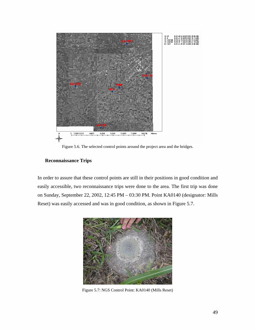
5.1 below. Using the info given in NGS datasheets, the map shown in Figure 5.6 is

created in ArcMap (ArcGIS) showing the control points, the Bridgeport Bridge and Six

Points Bridge. The images used in the background are the aerial orthophotos of the area,

acquired from the CAAGIS website (http://pasture.ecn.purdue.edu/~caagis/).

Figure 5.1: Map of KA0140 Figure 5.2: Map of KA0159

48

Figure 5.3: Map of KA1653 Figure 5.4: Map of KA1958

Figure 5.5. Control points around the project area and the bridge locations.

Table 5.1: Order of Control Points (source: www.ngs.noaa.gov)

PID Horizontal Vertical

KA0140 Order B (second best) Unknown Stability

KA0159 Order B (second best) Order 2 (second best)

KA1653 Order B (second best) Order 1 (the best)

KA1958 Order 1 (third best) Unknown Stability

49

Figure 5.6. The selected control points around the project area and the bridges.

Reconnaissance Trips

In order to assure that these control points are still in their positions in good condition and

easily accessible, two reconnaissance trips were done to the area. The first trip was done

on Sunday, September 22, 2002, 12:45 PM – 03:30 PM. Point KA0140 (designator: Mills

Reset) was easily accessed and was in good condition, as shown in Figure 5.7.

Figure 5.7: NGS Control Point: KA0140 (Mills Reset)

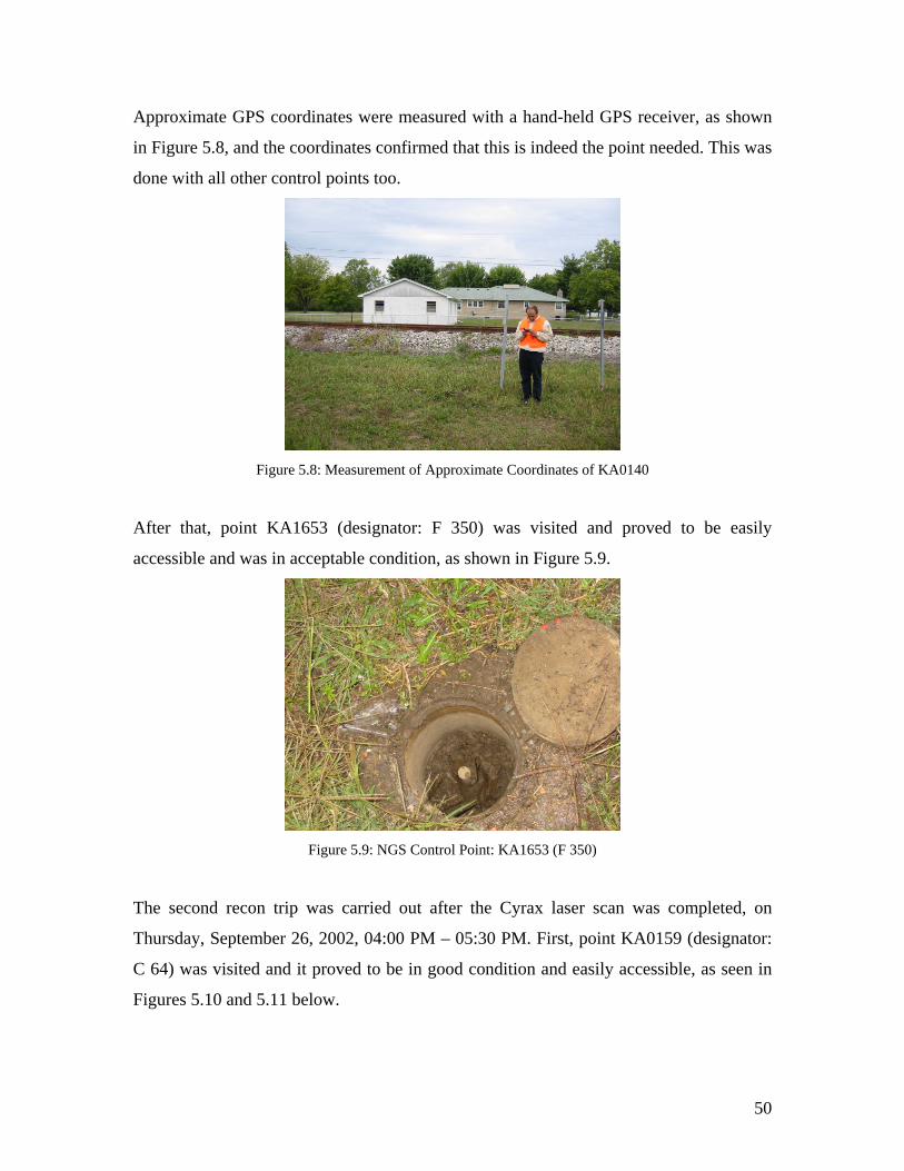
50

Approximate GPS coordinates were measured with a hand-held GPS receiver, as shown

in Figure 5.8, and the coordinates confirmed that this is indeed the point needed. This was

done with all other control points too.

Figure 5.8: Measurement of Approximate Coordinates of KA0140

After that, point KA1653 (designator: F 350) was visited and proved to be easily

accessible and was in acceptable condition, as shown in Figure 5.9.

Figure 5.9: NGS Control Point: KA1653 (F 350)

The second recon trip was carried out after the Cyrax laser scan was completed, on

Thursday, September 26, 2002, 04:00 PM – 05:30 PM. First, point KA0159 (designator:

C 64) was visited and it proved to be in good condition and easily accessible, as seen in

Figures 5.10 and 5.11 below.

51

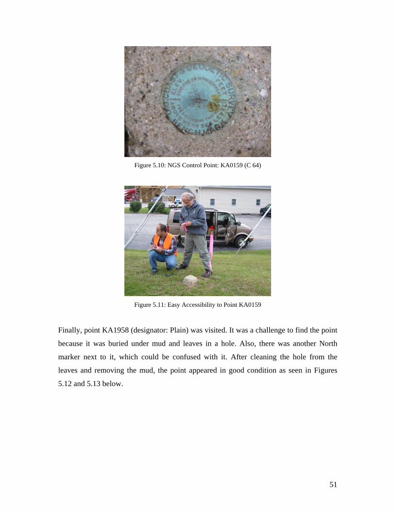
Figure 5.10: NGS Control Point: KA0159 (C 64)

Figure 5.11: Easy Accessibility to Point KA0159

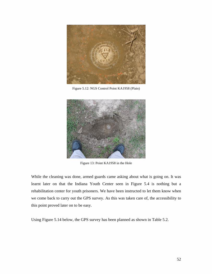
Finally, point KA1958 (designator: Plain) was visited. It was a challenge to find the point

because it was buried under mud and leaves in a hole. Also, there was another North

marker next to it, which could be confused with it. After cleaning the hole from the

leaves and removing the mud, the point appeared in good condition as seen in Figures

5.12 and 5.13 below.

52

Figure 5.12: NGS Control Point KA1958 (Plain)

Figure 13: Point KA1958 in the Hole

While the cleaning was done, armed guards came asking about what is going on. It was

learnt later on that the Indiana Youth Center seen in Figure 5.4 is nothing but a

rehabilitation center for youth prisoners. We have been instructed to let them know when

we come back to carry out the GPS survey. As this was taken care of, the accessibility to

this point proved later on to be easy.

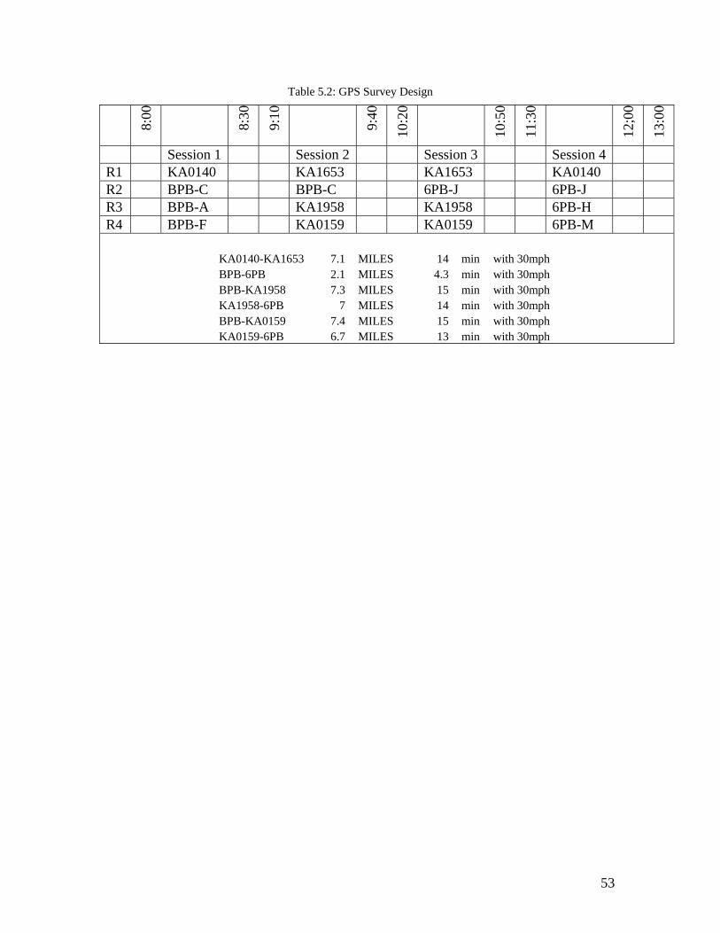
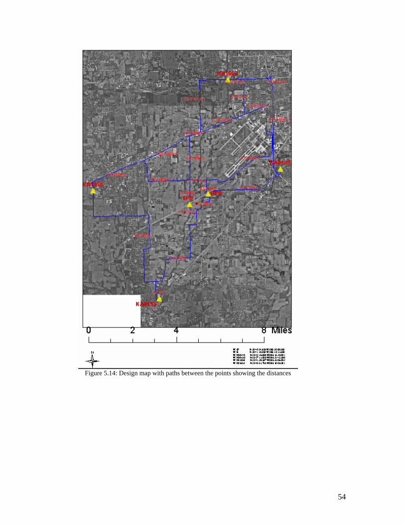
Using Figure 5.14 below, the GPS survey has been planned as shown in Table 5.2.

53

Table 5.2: GPS Survey Design

8:00

8:

30

9:10

9:40

10:2

0

10:5

0

11:3

0

12;0

0

13:0

0

Session 1 Session 2 Session 3 Session 4 R1 KA0140 KA1653 KA1653 KA0140 R2 BPB-C BPB-C 6PB-J 6PB-J R3 BPB-A KA1958 KA1958 6PB-H R4 BPB-F KA0159 KA0159 6PB-M

KA0140-KA1653 7.1 MILES 14 min with 30mph BPB-6PB 2.1 MILES 4.3 min with 30mph BPB-KA1958 7.3 MILES 15 min with 30mph KA1958-6PB 7 MILES 14 min with 30mph BPB-KA0159 7.4 MILES 15 min with 30mph KA0159-6PB 6.7 MILES 13 min with 30mph

54

Figure 5.14: Design map with paths between the points showing the distances

55

The GPS Survey

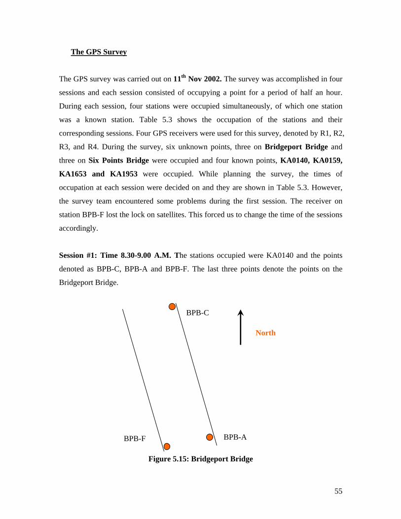
The GPS survey was carried out on 11th Nov 2002. The survey was accomplished in four

sessions and each session consisted of occupying a point for a period of half an hour.

During each session, four stations were occupied simultaneously, of which one station

was a known station. Table 5.3 shows the occupation of the stations and their

corresponding sessions. Four GPS receivers were used for this survey, denoted by R1, R2,

R3, and R4. During the survey, six unknown points, three on Bridgeport Bridge and

three on Six Points Bridge were occupied and four known points, KA0140, KA0159,

KA1653 and KA1953 were occupied. While planning the survey, the times of

occupation at each session were decided on and they are shown in Table 5.3. However,

the survey team encountered some problems during the first session. The receiver on

station BPB-F lost the lock on satellites. This forced us to change the time of the sessions

accordingly.

Session #1: Time 8.30-9.00 A.M. The stations occupied were KA0140 and the points

denoted as BPB-C, BPB-A and BPB-F. The last three points denote the points on the

Bridgeport Bridge.

Figure 5.15: Bridgeport Bridge

BPB-C

BPB-A BPB-F

North

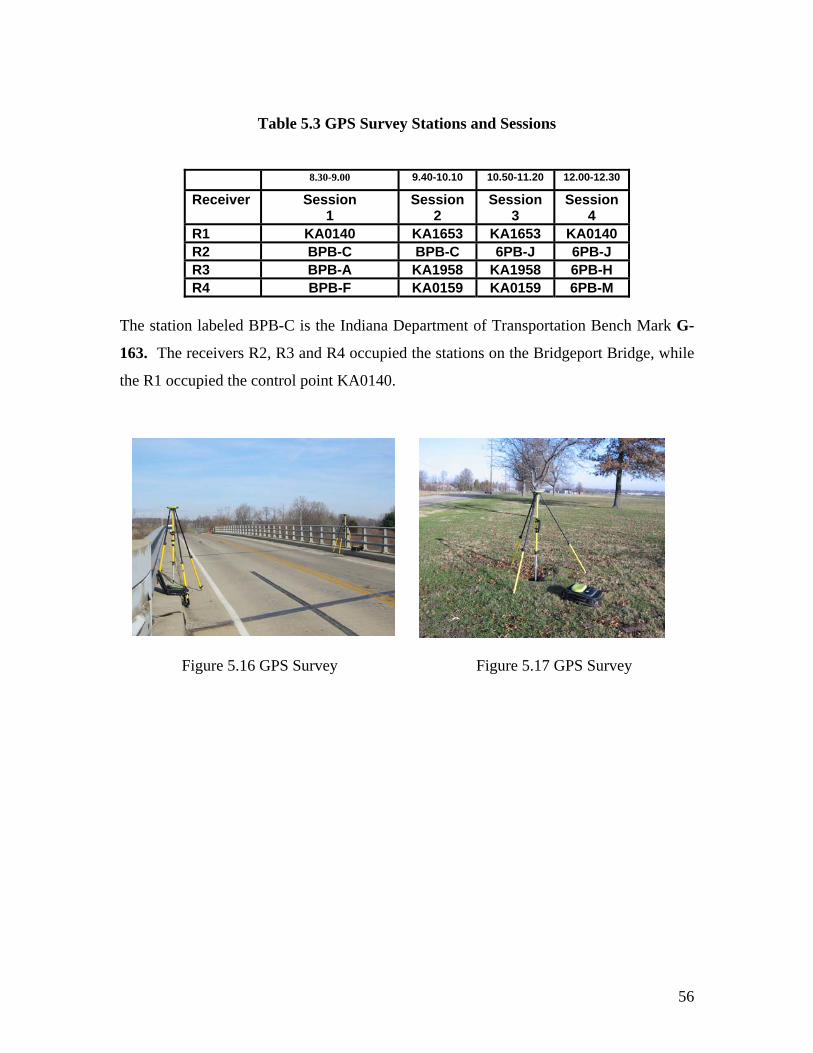
56

Table 5.3 GPS Survey Stations and Sessions

8.30-9.00 9.40-10.10 10.50-11.20 12.00-12.30

Receiver Session 1

Session 2

Session 3

Session 4

R1 KA0140 KA1653 KA1653 KA0140 R2 BPB-C BPB-C 6PB-J 6PB-J R3 BPB-A KA1958 KA1958 6PB-H R4 BPB-F KA0159 KA0159 6PB-M

The station labeled BPB-C is the Indiana Department of Transportation Bench Mark G-

163. The receivers R2, R3 and R4 occupied the stations on the Bridgeport Bridge, while

the R1 occupied the control point KA0140.

Figure 5.16 GPS Survey Figure 5.17 GPS Survey

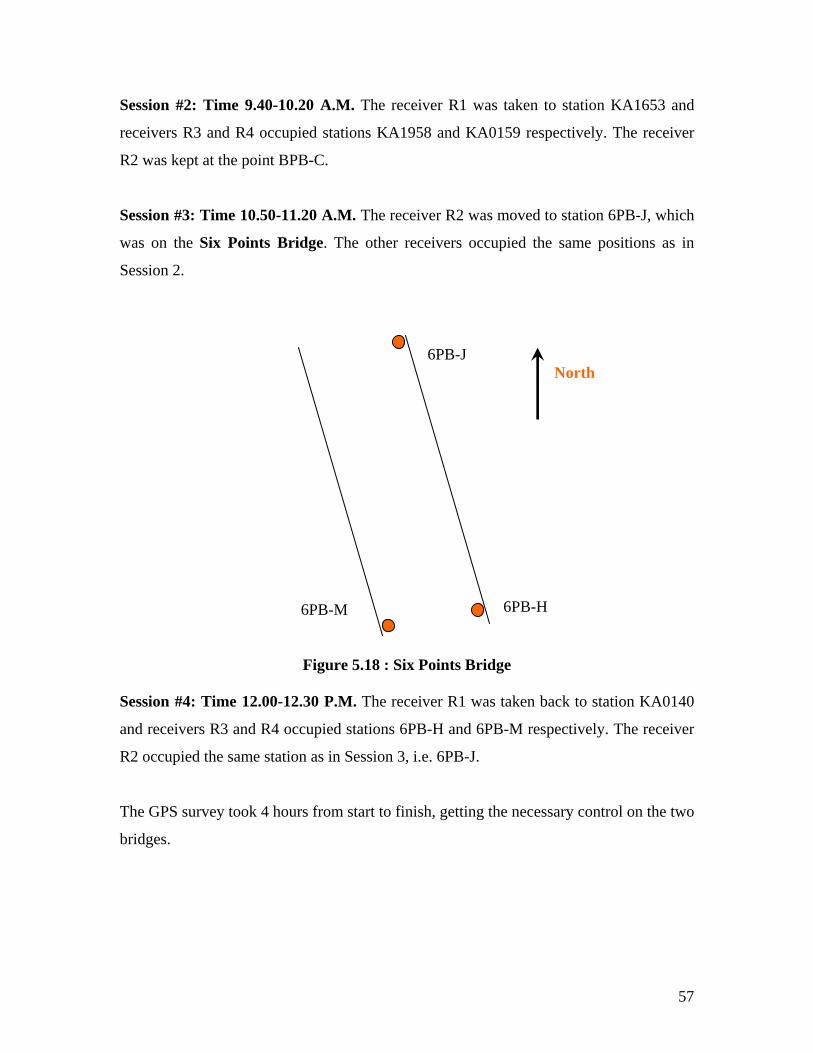
57

Session #2: Time 9.40-10.20 A.M. The receiver R1 was taken to station KA1653 and

receivers R3 and R4 occupied stations KA1958 and KA0159 respectively. The receiver

R2 was kept at the point BPB-C.

Session #3: Time 10.50-11.20 A.M. The receiver R2 was moved to station 6PB-J, which

was on the Six Points Bridge. The other receivers occupied the same positions as in

Session 2.

Figure 5.18 : Six Points Bridge Session #4: Time 12.00-12.30 P.M. The receiver R1 was taken back to station KA0140

and receivers R3 and R4 occupied stations 6PB-H and 6PB-M respectively. The receiver

R2 occupied the same station as in Session 3, i.e. 6PB-J.

The GPS survey took 4 hours from start to finish, getting the necessary control on the two

bridges.

North

6PB-M

6PB-J

6PB-H

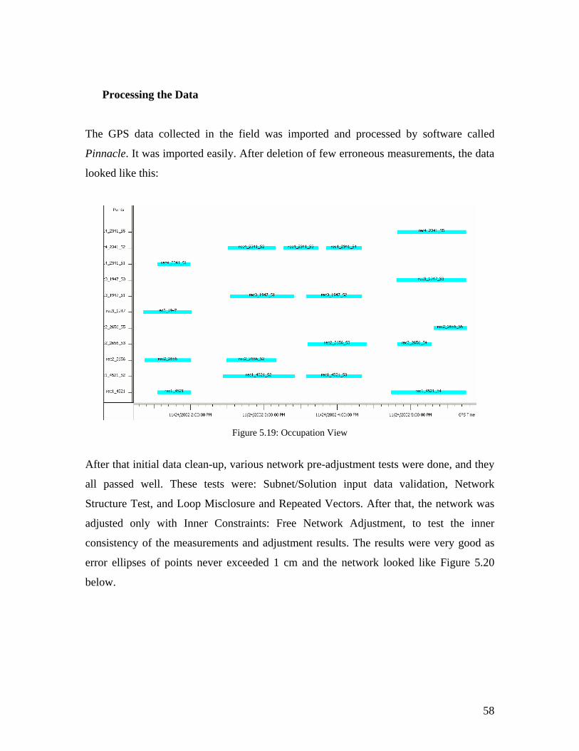
58

Processing the Data

The GPS data collected in the field was imported and processed by software called

Pinnacle. It was imported easily. After deletion of few erroneous measurements, the data

looked like this:

Figure 5.19: Occupation View

After that initial data clean-up, various network pre-adjustment tests were done, and they

all passed well. These tests were: Subnet/Solution input data validation, Network

Structure Test, and Loop Misclosure and Repeated Vectors. After that, the network was

adjusted only with Inner Constraints: Free Network Adjustment, to test the inner

consistency of the measurements and adjustment results. The results were very good as

error ellipses of points never exceeded 1 cm and the network looked like Figure 5.20

below.

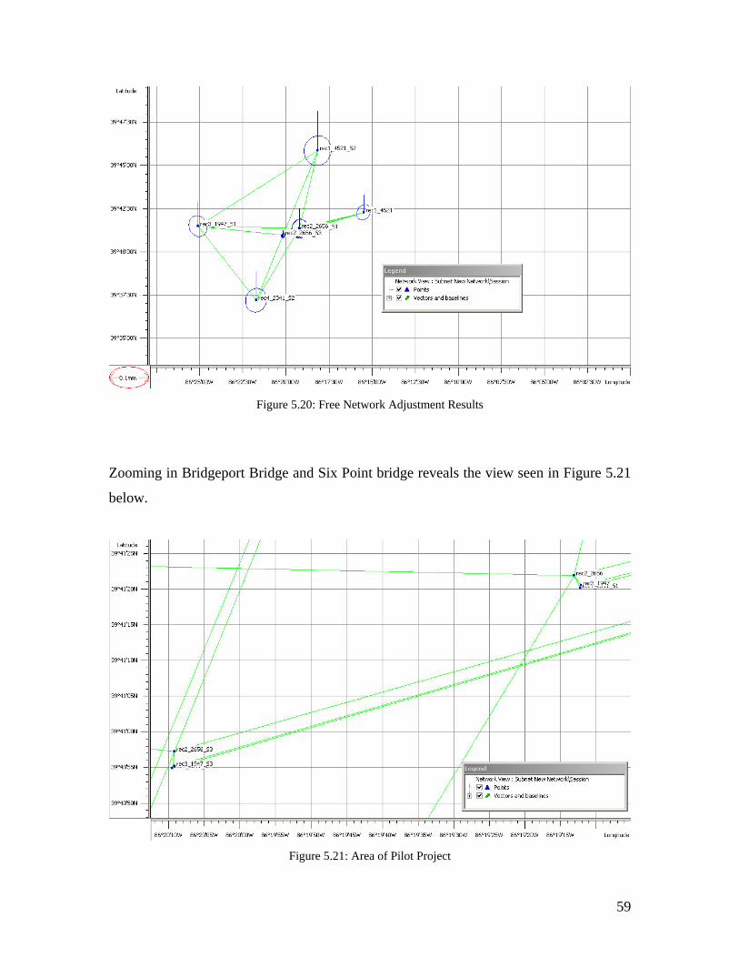
59

Figure 5.20: Free Network Adjustment Results

Zooming in Bridgeport Bridge and Six Point bridge reveals the view seen in Figure 5.21

below.

Figure 5.21: Area of Pilot Project

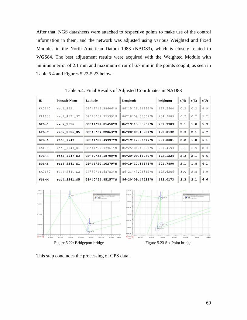
60

After that, NGS datasheets were attached to respective points to make use of the control

information in them, and the network was adjusted using various Weighted and Fixed

Modules in the North American Datum 1983 (NAD83), which is closely related to

WGS84. The best adjustment results were acquired with the Weighted Module with

minimum error of 2.1 mm and maximum error of 6.7 mm in the points sought, as seen in

Table 5.4 and Figures 5.22-5.23 below.

Table 5.4: Final Results of Adjusted Coordinates in NAD83

ID Pinnacle Name Latitude Longitude height(m) s(N) s(E) s(U)

KA0140 rec1_4521 39°42'16.98646"N 86°15'29.31895"W 197.5604 0.2 0.2 4.9

KA1653 rec1_4521_S2 39°45'51.75539"N 86°18'09.38069"W 204.9889 0.2 0.2 5.2

BPB-C rec2_2656 39°41'21.85450"N 86°19'13.03939"W 201.7783 2.1 1.8 5.9

6PB-J rec2_2656_S5 39°40'57.22863"N 86°20'09.18901"W 192.0132 2.3 2.1 6.7

BPB-A rec3_1947 39°41'20.49997"N 86°19'12.06519"W 201.8801 2.2 1.8 6.1

KA1958 rec3_1947_S1 39°41'29.33961"N 86°25'06.45938"W 207.4593 3.1 2.9 8.3

6PB-H rec3_1947_S3 39°40'55.18700"N 86°20'09.16070"W 192.1224 2.3 2.1 6.6

BPB-F rec4_2341_S1 39°41'20.10279"N 86°19'12.14378"W 201.7890 2.1 1.8 6.1

KA0159 rec4_2341_S2 39°37'11.68783"N 86°21'43.96842"W 172.6206 3.0 2.8 4.9

6PB-M rec4_2341_S5 39°40'54.85157"N 86°20'09.47523"W 192.0173 2.3 2.1 6.6

Figure 5.22: Bridgeport bridge Figure 5.23 Six Point bridge

This step concludes the processing of GPS data.

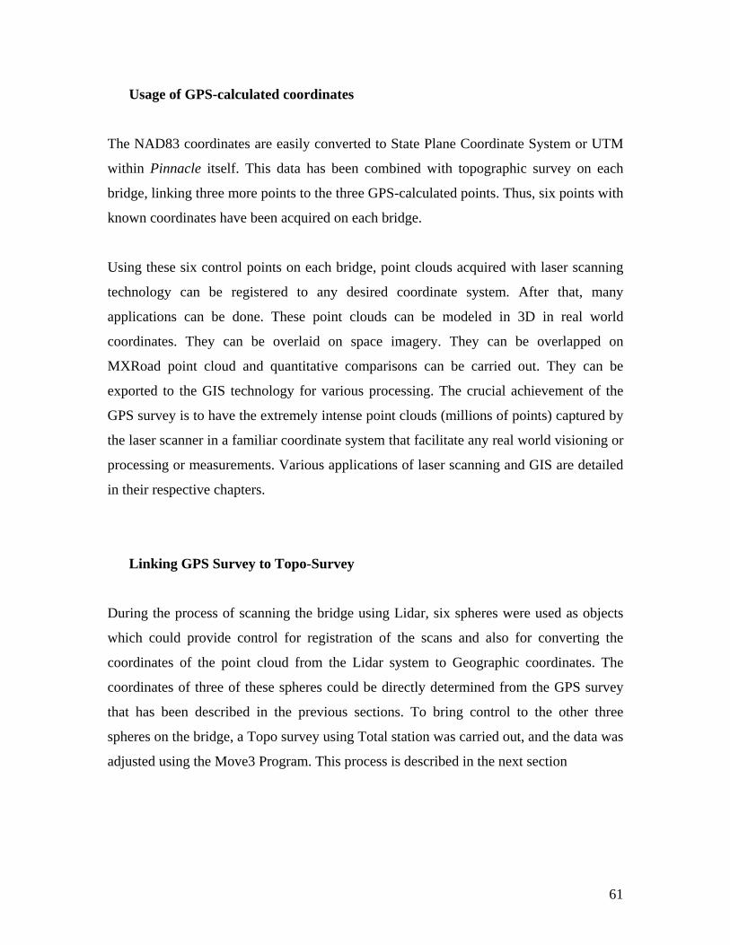
61

Usage of GPS-calculated coordinates

The NAD83 coordinates are easily converted to State Plane Coordinate System or UTM

within Pinnacle itself. This data has been combined with topographic survey on each

bridge, linking three more points to the three GPS-calculated points. Thus, six points with

known coordinates have been acquired on each bridge.

Using these six control points on each bridge, point clouds acquired with laser scanning

technology can be registered to any desired coordinate system. After that, many

applications can be done. These point clouds can be modeled in 3D in real world

coordinates. They can be overlaid on space imagery. They can be overlapped on

MXRoad point cloud and quantitative comparisons can be carried out. They can be

exported to the GIS technology for various processing. The crucial achievement of the

GPS survey is to have the extremely intense point clouds (millions of points) captured by

the laser scanner in a familiar coordinate system that facilitate any real world visioning or

processing or measurements. Various applications of laser scanning and GIS are detailed

in their respective chapters.

Linking GPS Survey to Topo-Survey

During the process of scanning the bridge using Lidar, six spheres were used as objects

which could provide control for registration of the scans and also for converting the

coordinates of the point cloud from the Lidar system to Geographic coordinates. The

coordinates of three of these spheres could be directly determined from the GPS survey

that has been described in the previous sections. To bring control to the other three

spheres on the bridge, a Topo survey using Total station was carried out, and the data was

adjusted using the Move3 Program. This process is described in the next section

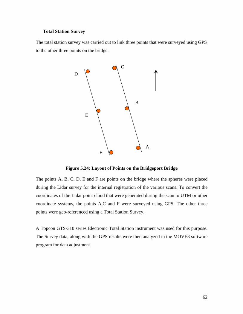
62

Total Station Survey The total station survey was carried out to link three points that were surveyed using GPS

to the other three points on the bridge.

Figure 5.24: Layout of Points on the Bridgeport Bridge The points A, B, C, D, E and F are points on the bridge where the spheres were placed

during the Lidar survey for the internal registration of the various scans. To convert the

coordinates of the Lidar point cloud that were generated during the scan to UTM or other

coordinate systems, the points A,C and F were surveyed using GPS. The other three

points were geo-referenced using a Total Station Survey.

A Topcon GTS-310 series Electronic Total Station instrument was used for this purpose.

The Survey data, along with the GPS results were then analyzed in the MOVE3 software

program for data adjustment.

F

C

A

E

D

B

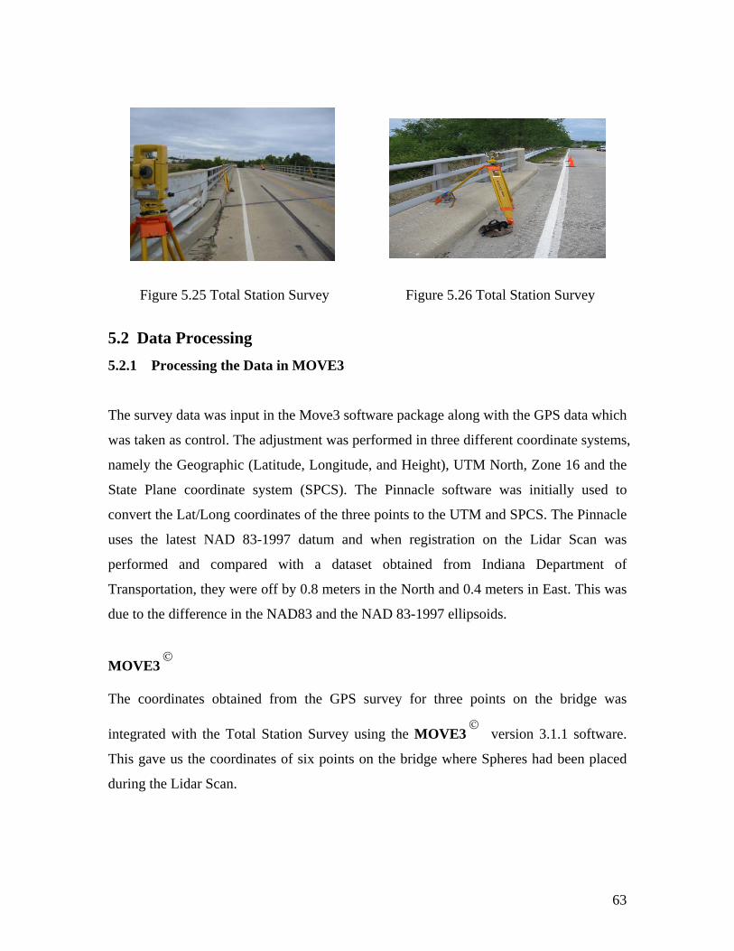
63

Figure 5.25 Total Station Survey Figure 5.26 Total Station Survey

5.2 Data Processing 5.2.1 Processing the Data in MOVE3

The survey data was input in the Move3 software package along with the GPS data which

was taken as control. The adjustment was performed in three different coordinate systems,

namely the Geographic (Latitude, Longitude, and Height), UTM North, Zone 16 and the

State Plane coordinate system (SPCS). The Pinnacle software was initially used to

convert the Lat/Long coordinates of the three points to the UTM and SPCS. The Pinnacle

uses the latest NAD 83-1997 datum and when registration on the Lidar Scan was

performed and compared with a dataset obtained from Indiana Department of

Transportation, they were off by 0.8 meters in the North and 0.4 meters in East. This was

due to the difference in the NAD83 and the NAD 83-1997 ellipsoids.

MOVE3©

The coordinates obtained from the GPS survey for three points on the bridge was

integrated with the Total Station Survey using the MOVE3©

version 3.1.1 software.

This gave us the coordinates of six points on the bridge where Spheres had been placed

during the Lidar Scan.

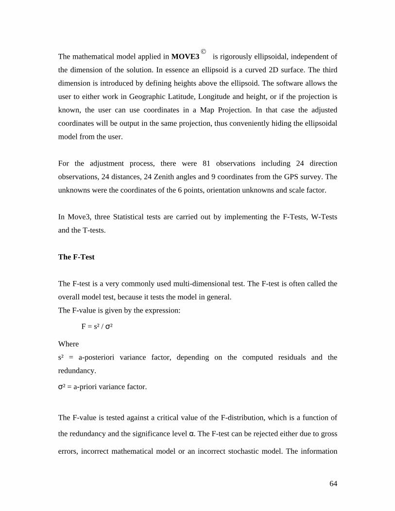
64

The mathematical model applied in MOVE3©

is rigorously ellipsoidal, independent of

the dimension of the solution. In essence an ellipsoid is a curved 2D surface. The third

dimension is introduced by defining heights above the ellipsoid. The software allows the

user to either work in Geographic Latitude, Longitude and height, or if the projection is

known, the user can use coordinates in a Map Projection. In that case the adjusted

coordinates will be output in the same projection, thus conveniently hiding the ellipsoidal

model from the user.

For the adjustment process, there were 81 observations including 24 direction

observations, 24 distances, 24 Zenith angles and 9 coordinates from the GPS survey. The

unknowns were the coordinates of the 6 points, orientation unknowns and scale factor.

In Move3, three Statistical tests are carried out by implementing the F-Tests, W-Tests

and the T-tests.

The F-Test

The F-test is a very commonly used multi-dimensional test. The F-test is often called the

overall model test, because it tests the model in general.

The F-value is given by the expression:

F = s² / σ²

Where

s² = a-posteriori variance factor, depending on the computed residuals and the

redundancy.

σ² = a-priori variance factor.

The F-value is tested against a critical value of the F-distribution, which is a function of

the redundancy and the significance level α. The F-test can be rejected either due to gross

errors, incorrect mathematical model or an incorrect stochastic model. The information

65

provided by the F-test, namely acceptance or rejection of the null-hypothesis is not very

specific. Therefore if the test is rejected, it is necessary to find the cause of the rejection

by tracing errors in observations or assumptions. A gross error is the observations will

then be revealed if a rejected F-Test is followed up by a W-Test. In our case, The F-test

was accepted at 0.048 (The ratio s² / σ²), against a critical value set at 1.10 (default value

in Move3).

A bug in the MOVE3 program prevented us from using the WGS84 ellipsoid that was

listed in their Pull down menu. This problem was a trivial one and was solved by using

the User defined ellipsoid and giving the parameters of the WGS84 ellipsoid as the input.

The program needed approximate coordinates for all the six points that were being

adjusted. Since three of the coordinates were known coordinates, obtained from the GPS

survey, an in-built COGO program calculated the approximate coordinates for the other 3

points.

Depending on the Input coordinates, the Adjustment output can be either in Geographic

Lat/Long or in a Map Projection system (e.g. SPCS or UTM). In the latter case, the

Projection needs to be defined before carrying out the adjustment process.

5.2.2 The Adjustment

The adjustment process in Move3 is a two step process. The first step is termed the Free

Network adjustment. In a free network adjustment, the geometrical layout is determined

by the observations only. The position, scale and orientation of the network are fixed by a

minimum number of constraints, through the base stations. Thus, the base stations impose

no extra constraints on the adjustment solution. The free network adjustment verified the

quality of the observations.

After the Free Network adjustment, we can either chose a Constrained adjustment, in

which case even the Base station coordinates (The Points surveyed using GPS) will

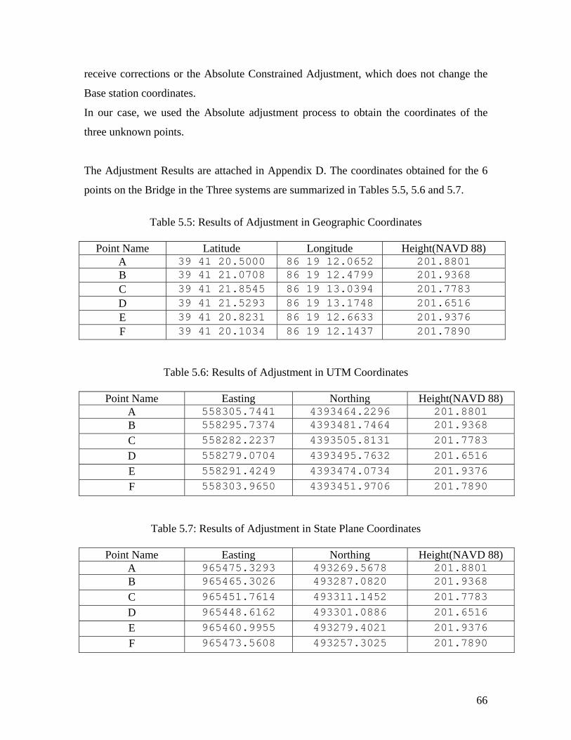
66

receive corrections or the Absolute Constrained Adjustment, which does not change the

Base station coordinates.

In our case, we used the Absolute adjustment process to obtain the coordinates of the

three unknown points.

The Adjustment Results are attached in Appendix D. The coordinates obtained for the 6

points on the Bridge in the Three systems are summarized in Tables 5.5, 5.6 and 5.7.

Table 5.5: Results of Adjustment in Geographic Coordinates

Point Name Latitude Longitude Height(NAVD 88)

A 39 41 20.5000 86 19 12.0652 201.8801 B 39 41 21.0708 86 19 12.4799 201.9368 C 39 41 21.8545 86 19 13.0394 201.7783 D 39 41 21.5293 86 19 13.1748 201.6516 E 39 41 20.8231 86 19 12.6633 201.9376 F 39 41 20.1034 86 19 12.1437 201.7890

Table 5.6: Results of Adjustment in UTM Coordinates

Point Name Easting Northing Height(NAVD 88) A 558305.7441 4393464.2296 201.8801 B 558295.7374 4393481.7464 201.9368 C 558282.2237 4393505.8131 201.7783 D 558279.0704 4393495.7632 201.6516 E 558291.4249 4393474.0734 201.9376 F 558303.9650 4393451.9706 201.7890

Table 5.7: Results of Adjustment in State Plane Coordinates

Point Name Easting Northing Height(NAVD 88) A 965475.3293 493269.5678 201.8801 B 965465.3026 493287.0820 201.9368 C 965451.7614 493311.1452 201.7783 D 965448.6162 493301.0886 201.6516 E 965460.9955 493279.4021 201.9376 F 965473.5608 493257.3025 201.7890

67

5.2.3 Ellipsoidal Heights to Ortho-metric Heights The heights in the three tables are ellipsoidal heights and these were used throughout the

Adjustment process because the Geoidal undulation for all the 6 points was a constant of

-32.995 meters in the GEOID96 system and -33.005 meters in the GEOID99 system. The

ellipsoidal heights were then converted to Orthometric heights. These coordinates were

then used to register the Lidar point cloud in the real world system of coordinates.

68

CHAPTER 6 Geographic Information System (GIS)

Simply put, a GIS combines layers of information about a place to give you a better

understanding of that place. What layers of information you combine depends on your

purpose—finding the best location for a new store, analyzing environmental damage,

viewing similar crimes in a city to detect a pattern, and so on.

The old adage "better information leads to better decisions" is true for GIS. A GIS is not

just an automated decision making system but a tool to query, analyze, and map data in

support of the decision making process.

One of the main benefits of GIS is improved management of your organization and

resources. A GIS can link data sets together by common locational data, such as

addresses, which helps departments and agencies share their data. By creating a shared

database, one department can benefit from the work of another—data can be collected

once and used many times.

A full GIS, or geographic information system, requires:

• Hardware (computers and peripherals) • Software • Data • People • Training

and sound analysis methods for interpreting the results generated by the GIS.

6.1 Introduction

This report presents the methodology of creating a geo-referenced 3D model and

visualization of project area. In order to do this, aerial images (DOQ), satellite photos,

digital elevation model (DEM), lidar data, and the MxRoads data are used. Over the

orthorectified aerial and satellite photos the MxRoads data and the lidar data of the

Bridgeport bridge are extruded using a DEM as the base terrain. The model can be

queried and navigated from ArcScene and ArcMap environment, the tools of ArcGIS

software.

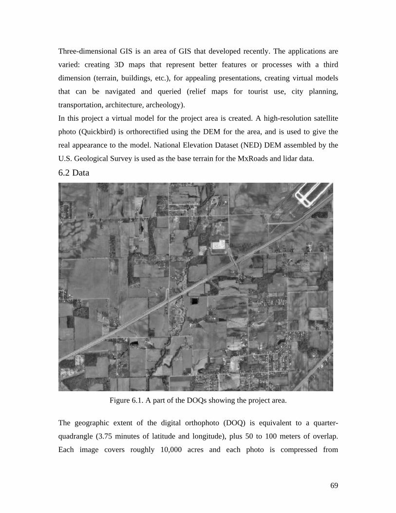
69

Three-dimensional GIS is an area of GIS that developed recently. The applications are

varied: creating 3D maps that represent better features or processes with a third

dimension (terrain, buildings, etc.), for appealing presentations, creating virtual models

that can be navigated and queried (relief maps for tourist use, city planning,

transportation, architecture, archeology).

In this project a virtual model for the project area is created. A high-resolution satellite

photo (Quickbird) is orthorectified using the DEM for the area, and is used to give the

real appearance to the model. National Elevation Dataset (NED) DEM assembled by the

U.S. Geological Survey is used as the base terrain for the MxRoads and lidar data.

6.2 Data

Figure 6.1. A part of the DOQs showing the project area.

The geographic extent of the digital orthophoto (DOQ) is equivalent to a quarter-

quadrangle (3.75 minutes of latitude and longitude), plus 50 to 100 meters of overlap.

Each image covers roughly 10,000 acres and each photo is compressed from

70

approximately 50 megabytes to 5 megabytes. The uncompressed resolution is 1 meter.

Resolution is the minimum distance between two adjacent features, or the minimum size

of a feature that can be detected by a remote sensing system. The quality of the image is

slightly degraded due to the compression in MrSID. The projection used for these photos

is Universal Transverse Mercator (UTM). The datum is the North American Datum of

1983 (NAD83), with coordinates in meters. The uncompressed orthophotos conform to

National Map Accuracy Standards at the scale of 1:12,000. This means that 90 percent of

the well-defined points tested must fall within 33.3 feet (1/30 inch at the original scale) of

their actual position. The compression may degrade this slightly. The images are

developed from aerial photos taken in 1998, with some from 1999. The 24 DOQs (Figure

6.1) used in this project are downloaded from Center for Advanced Applications in

Geographic Information Systems (CAAGIS) website

(http://danpatch.ecn.purdue.edu/~caagis/ftp/gisdata/data.html).

The National Elevation Dataset (NED) is a new raster product assembled by the U.S.

Geological Survey. NED is designed to provide National elevation data in a seamless

form with a consistent datum, elevation unit, and projection. Data corrections were made

in the NED assembly process to minimize artifacts, perform edge matching, and fill sliver

areas of missing data. NED has a resolution of one arc-second (approximately 30 meters)

for the conterminous United States, Hawaii, and Puerto Rico and a resolution of two arc-

seconds for Alaska. NED data sources have a variety of elevation units, horizontal

datums, and map projections. In the NED assembly process the elevation values are

converted to decimal meters as a consistent unit of measure, NAD83 is consistently used

as horizontal datum, and all the data are recast in a geographic projection. The NED data

(Figure 6.2) in UTM is acquired from the GIS lab at Purdue University Civil Engineering

Department, Geomatics Engineering Program. The data covers an area of 905 square

kilometers and is 4.4 MBs. Other than NED DEM InfSAR DEMs can also be used but

currently no InfSAR data is available for the project area.

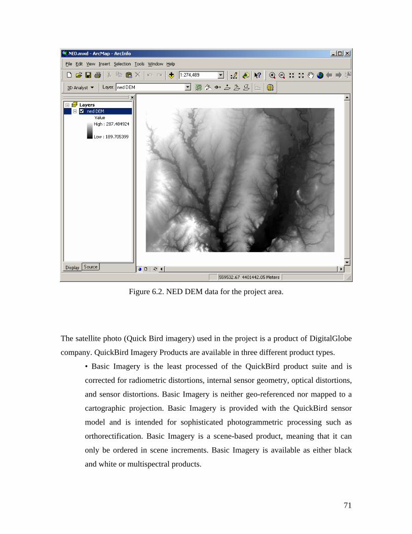
71

Figure 6.2. NED DEM data for the project area.

The satellite photo (Quick Bird imagery) used in the project is a product of DigitalGlobe

company. QuickBird Imagery Products are available in three different product types.

• Basic Imagery is the least processed of the QuickBird product suite and is

corrected for radiometric distortions, internal sensor geometry, optical distortions,

and sensor distortions. Basic Imagery is neither geo-referenced nor mapped to a

cartographic projection. Basic Imagery is provided with the QuickBird sensor

model and is intended for sophisticated photogrammetric processing such as

orthorectification. Basic Imagery is a scene-based product, meaning that it can

only be ordered in scene increments. Basic Imagery is available as either black

and white or multispectral products.

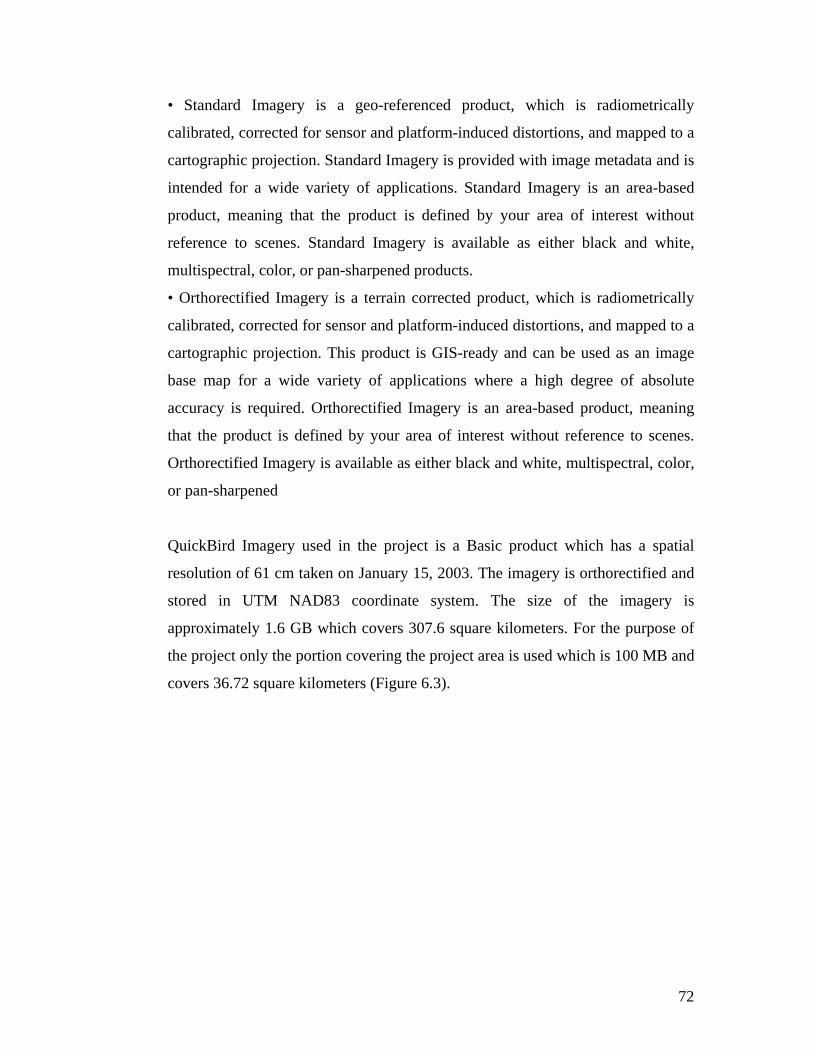
72

• Standard Imagery is a geo-referenced product, which is radiometrically

calibrated, corrected for sensor and platform-induced distortions, and mapped to a

cartographic projection. Standard Imagery is provided with image metadata and is

intended for a wide variety of applications. Standard Imagery is an area-based

product, meaning that the product is defined by your area of interest without

reference to scenes. Standard Imagery is available as either black and white,

multispectral, color, or pan-sharpened products.

• Orthorectified Imagery is a terrain corrected product, which is radiometrically

calibrated, corrected for sensor and platform-induced distortions, and mapped to a

cartographic projection. This product is GIS-ready and can be used as an image

base map for a wide variety of applications where a high degree of absolute

accuracy is required. Orthorectified Imagery is an area-based product, meaning

that the product is defined by your area of interest without reference to scenes.

Orthorectified Imagery is available as either black and white, multispectral, color,

or pan-sharpened

QuickBird Imagery used in the project is a Basic product which has a spatial

resolution of 61 cm taken on January 15, 2003. The imagery is orthorectified and

stored in UTM NAD83 coordinate system. The size of the imagery is

approximately 1.6 GB which covers 307.6 square kilometers. For the purpose of

the project only the portion covering the project area is used which is 100 MB and

covers 36.72 square kilometers (Figure 6.3).

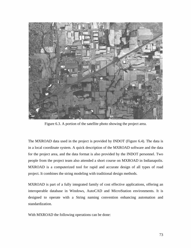
73

Figure 6.3. A portion of the satellite photo showing the project area.

The MXROAD data used in the project is provided by INDOT (Figure 6.4). The data is

in a local coordinate system. A quick description of the MXROAD software and the data

for the project area, and the data format is also provided by the INDOT personnel. Two

people from the project team also attended a short course on MXROAD in Indianapolis.

MXROAD is a computerized tool for rapid and accurate design of all types of road

project. It combines the string modeling with traditional design methods.

MXROAD is part of a fully integrated family of cost effective applications, offering an

interoperable database in Windows, AutoCAD and MicroStation environments. It is

designed to operate with a String naming convention enhancing automation and

standardization.

With MXROAD the following operations can be done:

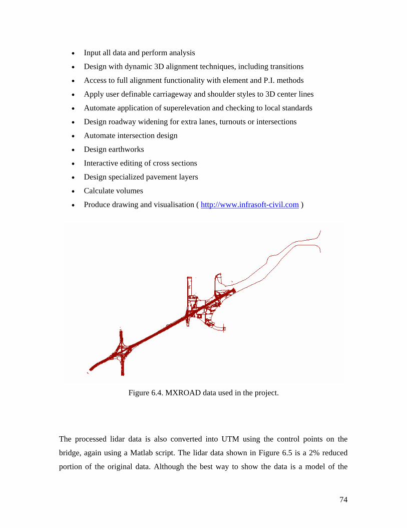
74

• Input all data and perform analysis

• Design with dynamic 3D alignment techniques, including transitions

• Access to full alignment functionality with element and P.I. methods

• Apply user definable carriageway and shoulder styles to 3D center lines

• Automate application of superelevation and checking to local standards

• Design roadway widening for extra lanes, turnouts or intersections

• Automate intersection design

• Design earthworks

• Interactive editing of cross sections

• Design specialized pavement layers

• Calculate volumes

• Produce drawing and visualisation ( http://www.infrasoft-civil.com )

Figure 6.4. MXROAD data used in the project.

The processed lidar data is also converted into UTM using the control points on the

bridge, again using a Matlab script. The lidar data shown in Figure 6.5 is a 2% reduced

portion of the original data. Although the best way to show the data is a model of the

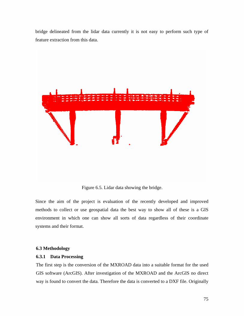
75

bridge delineated from the lidar data currently it is not easy to perform such type of

feature extraction from this data.

Figure 6.5. Lidar data showing the bridge.

Since the aim of the project is evaluation of the recently developed and improved

methods to collect or use geospatial data the best way to show all of these is a GIS

environment in which one can show all sorts of data regardless of their coordinate

systems and their format.

6.3 Methodology

6.3.1 Data Processing

The first step is the conversion of the MXROAD data into a suitable format for the used

GIS software (ArcGIS). After investigation of the MXROAD and the ArcGIS no direct

way is found to convert the data. Therefore the data is converted to a DXF file. Originally

76

the MXROAD data consists of strings which describe the data for the software. When the

data is converted to DXF it has point, text, and line features in it. To preserve the 3rd

dimension of the features and to use them appropriately in ArcGIS the DXF file is

converted to a proper text file which can be imported into ArcGIS. The conversion is

done by writing a script in Matlab software. Although the ArcGIS can show all data in

different coordinate systems at once, the data is converted into UTM NAD83 coordinate

system to prevent any misinterpretation of the data. The conversion is done by using the

control points used in GPS analysis which are given in the documentation (Appendix C)

provided by the company that produced the MXROAD data. ArcGIS allows users to keep

the metadata information with the data itself. This ability provides the status of the data,

time period for which data is relevant, publication information, spatial data description,

and the description of the attributes of the data.

The lidar data processed by the Cyclone software is reduced to a 2% of the original one

to visualize the data faster in ArcGIS, converted into UTM and imported as a shapefile.

The satellite imagery is also rectified in UTM and saved as “satimagery.tif” which can be

found in the provided CDrom.

Figure 6.6 shows the data used in the project all together in one view.

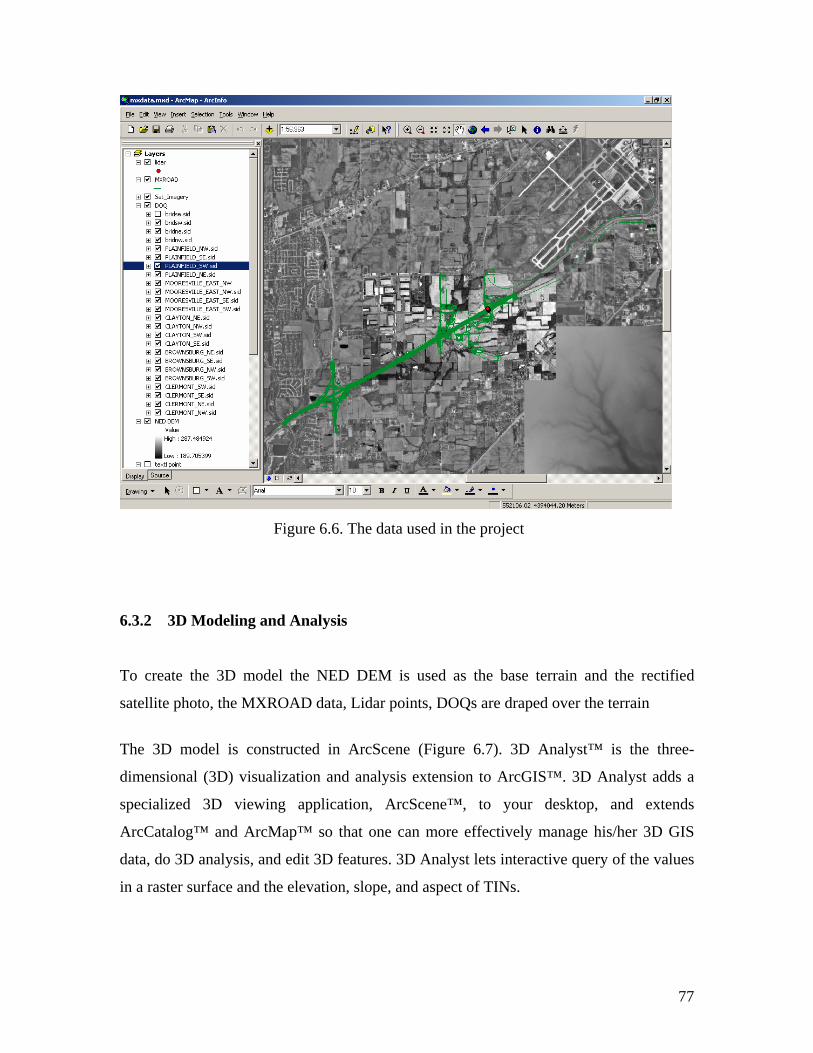
77

Figure 6.6. The data used in the project

6.3.2 3D Modeling and Analysis

To create the 3D model the NED DEM is used as the base terrain and the rectified

satellite photo, the MXROAD data, Lidar points, DOQs are draped over the terrain

The 3D model is constructed in ArcScene (Figure 6.7). 3D Analyst™ is the three-

dimensional (3D) visualization and analysis extension to ArcGIS™. 3D Analyst adds a

specialized 3D viewing application, ArcScene™, to your desktop, and extends

ArcCatalog™ and ArcMap™ so that one can more effectively manage his/her 3D GIS

data, do 3D analysis, and edit 3D features. 3D Analyst lets interactive query of the values

in a raster surface and the elevation, slope, and aspect of TINs.

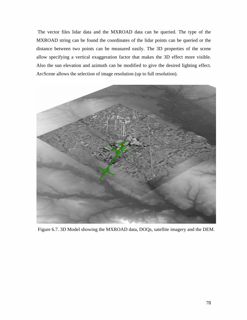
78

The vector files lidar data and the MXROAD data can be queried. The type of the

MXROAD string can be found the coordinates of the lidar points can be queried or the

distance between two points can be measured easily. The 3D properties of the scene

allow specifying a vertical exaggeration factor that makes the 3D effect more visible.

Also the sun elevation and azimuth can be modified to give the desired lighting effect.

ArcScene allows the selection of image resolution (up to full resolution).

Figure 6.7. 3D Model showing the MXROAD data, DOQs, satellite imagery and the DEM.

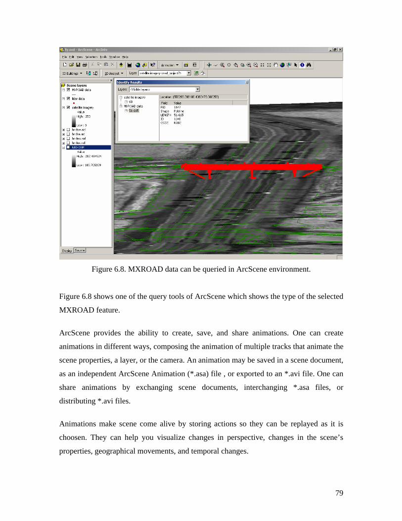
79

Figure 6.8. MXROAD data can be queried in ArcScene environment.

Figure 6.8 shows one of the query tools of ArcScene which shows the type of the selected

MXROAD feature.

ArcScene provides the ability to create, save, and share animations. One can create

animations in different ways, composing the animation of multiple tracks that animate the

scene properties, a layer, or the camera. An animation may be saved in a scene document,

as an independent ArcScene Animation (*.asa) file , or exported to an *.avi file. One can

share animations by exchanging scene documents, interchanging *.asa files, or

distributing *.avi files.

Animations make scene come alive by storing actions so they can be replayed as it is

choosen. They can help you visualize changes in perspective, changes in the scene’s

properties, geographical movements, and temporal changes.

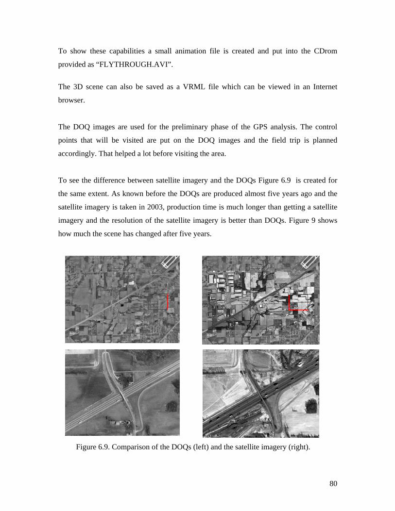
80

To show these capabilities a small animation file is created and put into the CDrom

provided as “FLYTHROUGH.AVI”.

The 3D scene can also be saved as a VRML file which can be viewed in an Internet

browser.

The DOQ images are used for the preliminary phase of the GPS analysis. The control

points that will be visited are put on the DOQ images and the field trip is planned

accordingly. That helped a lot before visiting the area.

To see the difference between satellite imagery and the DOQs Figure 6.9 is created for

the same extent. As known before the DOQs are produced almost five years ago and the

satellite imagery is taken in 2003, production time is much longer than getting a satellite

imagery and the resolution of the satellite imagery is better than DOQs. Figure 9 shows

how much the scene has changed after five years.

Figure 6.9. Comparison of the DOQs (left) and the satellite imagery (right).

81

6.4 Results

Using satellite imagery instead of aerial photos can provide faster results to investigate

the project area.

Conversion of the MXROAD data into the ArcGIS system is not easy, but it is hoped that

this problem can be solved very easily. The lidar point cloud should be processed and a

CAD model of the data should be obtained to obtain more useful information.

Surveyors and engineers understand the importance of geographic data. Surveyors use

precise instruments, procedures, and computations to accurately locate and define

geographic features while conducting field surveys that range from cadastral to

engineering construction layout. Engineers design and build structures and infrastructures

on geography measured by surveyors.

A GIS provides tools to help surveyors integrate a variety of data sources and types,

maintain and manage inventories, visualize data and related information using dynamic

maps, make decisions about resource management, and perform modeling and analysis.

The expansion of GIS technology has led to the development of new tools created

specifically for surveyors and engineers.

GIS can be used to determine the location of an event or asset and its relationship or

proximity to another event or asset, which may be the critical factor leading to a decision

about design, construction, or maintenance. The cost of feature maintenance and asset

inventory creation may be significantly reduced through the use of automated data

collection and software tools

GIS helps organize bridge management information contained in various forms, such as

inspection reports, rehab plans, and CAD files. Maintenance management and asset

valuation may be enhanced with GIS and linear referencing systems.

82

CHAPTER 7 Conclusions

Design data collection involving the use of Lidar instrument, in conjunction with GPS

proves to be a very effective. Data required to model two bridges was collected on a

single day, involving five-six sessions with the instrument. Even though the data was

collected on two bridges over the I-70, it did not cause any disruption of the traffic, either

on the Interstate or on the bridges. A major cause of concern during such activities,

particularly along interstates can be safety, both for the motorists as well as the people

involved in data collection. Lidar data collection was found to be extremely safe in both

these respects.

The whole process of collecting the Lidar data and the GPS coordinates for control was

completed in 2 days for both the bridges. Office work involved combining the GPS data

with conventional survey data to bring control on six pre-selected within the lidar point

cloud. This control information was later used to bring the point cloud to a geographic

coordinate system.

This provided us with means to compare the 3D point cloud with the bridge designs that

were created using other methods of data collection. It was found that the 3D point cloud

exhibits a very high degree of accuracy, both internally and also when geo-referenced

independently using GPS and conventional control survey. The lidar model was also

compared to the MXRoad data model provided by INDOT. The discrepancies between

the two models were not larger than 0.125 ft/3.81 cm and 0.05 ft/1.52 cm in the

horizontal and vertical planes respectively.

The data collected could completely model the bridge and the accuracy of the data

ensures that any models of the bridge, either as a whole or in part, will correctly reflect

the current state of the bridge.

As shown in section 3.6, the data collected can be used for various applications including

cut-and-fill estimates, modeling the state of the bridge, making measurements on various

parts of the bridge etc.

83

A cause of concern is the amount of data involved. As millions of 3D points are

collected, popular CAD/GIS packages are unable to deal with it. For this reason

proprietary software, designed particularly to handle such huge volumes of data involved,

was used for analyzing this data. However, it is possible to export data from this software

to other commonly used CAD packages.

Using satellite imagery instead of aerial photos can provide faster results to investigate

the project area.

Conversion of the MXROAD data into the ArcGIS system is not easy, but it is hoped that

this problem can be solved very easily. The lidar point cloud should be processed and a

CAD model of the data should be obtained to obtain more useful information.

With the help of the GIS a variety of data sources and types can be integrated, visualized

and used to make about resource management, and perform modeling and analysis. GIS

helps organize bridge management information contained in various forms, such as

inspection reports, rehab plans, and CAD files. Maintenance management and asset

valuation may be enhanced with GIS and linear referencing systems

FINAL REPORT

FWHA/IN/JTRP-2003-13

MODERN TECHNOLOGIES FOR DESIGN DATA COLLECTION

By

James S. Bethel Steven D. Johnson

Jie Shan Boudewijn H.W. van Gelder

Professors of Civil Engineering and

Bob McCullouch Research Scientist

Ali Fuat Cetin Seungwoo Han Mosab Hawarey

Changno Lee Aparajithan Sampath

Graduate Research Assistants

School of Civil Engineering Purdue University

Joint Transportation Research Program Project No: C-36-67PPP

File No: 9-10-67 SPR-2450

Conducted in Cooperation with the

Indiana Department of Transportation and the

U.S. Department of Transportation Federal Highway Administration

The contents of this report reflect the views of the authors, who are responsible for the facts and the accuracy of the data presented herein. The contents do not necessarily reflect the official views or policies of the Indiana Department of Transportation or the Federal Highway Administration at the time of publication. The report does not constitute a standard, specification, or regulation.

Purdue University

West Lafayette, IN 47907 August 2005

130

REFERENCES Chapter 2 http://ntl.bts.gov/DOCS/96134/ch03/body_ch03_03.html Indiana Department of Transportation Consulting Services Procedures MX Road Manual Version 2.5 Joint Transportation Research Program (http://rebar.ecn.purdue.edu/JTRP/ ) Indiana Department of Transportation (INDOT) (http://www.state.in.us/dot/) Chapter 3 http://www.optech.on.ca http://www.falk-pli.com http://www.cyra.com http://www.innovmetric.com http://www.move3.com http://www.cadapult-software.com Chapter 4 IKONOS Official Web Site ( http://www.spaceimaging.com) QuickBird Official Web Site (http://www.digitalglobe.com/) Chapter 5 National Geodetic Survey (NGS): www.ngs.noaa.gov

Chapter 6

Center for Advanced Applications in Geographic Information Systems (CAAGIS)

website (http://danpatch.ecn.purdue.edu/~caagis/ftp/gisdata/data.html).

http://www.infrasoft-civil.com http://www.esri.com

84

APPENDIX A

Lidar Movie A flythrough movie which shows the data used and produced in the project which includes the DEM, satellite images and Lidar point clouds in a 3D environment.

SEE CD IN BACK COVER OF REPORT

85

APPENDIX B

Gis Data Movie A more detailed flythrough movie which shows the data used and produced in the project which includes the DEM, satellite images and Lidar point clouds of the Bridgeport bridge in a 3D environment.


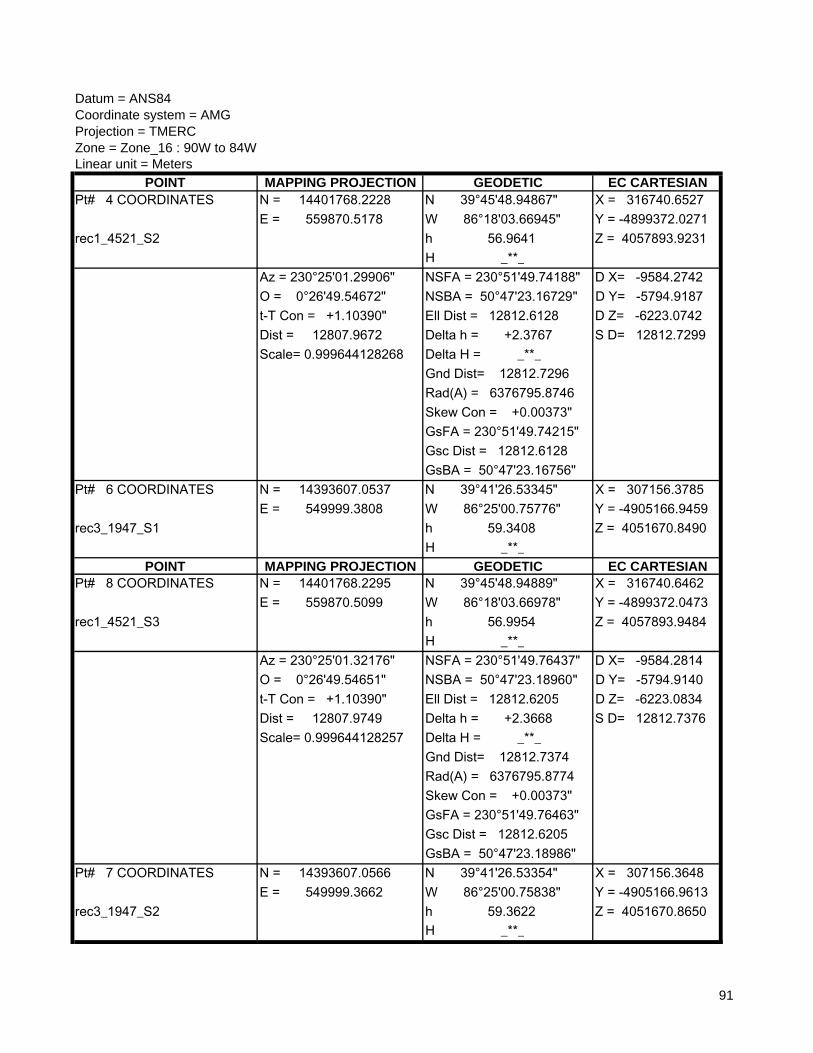
Datum = ANS84Coordinate system = AMGProjection = TMERCZone = Zone_16 : 90W to 84WLinear unit = Meters

POINT MAPPING PROJECTION GEODETIC EC CARTESIANPt# 4 COORDINATES N = 14401768.2228 N 39°45'48.94867" X = 316740.6527 E = 559870.5178 W 86°18'03.66945" Y = -4899372.0271rec1_4521_S2 h 56.9641 Z = 4057893.9231 H _**_ Az = 230°25'01.29906" NSFA = 230°51'49.74188" D X= -9584.2742 O = 0°26'49.54672" NSBA = 50°47'23.16729" D Y= -5794.9187 t-T Con = +1.10390" Ell Dist = 12812.6128 D Z= -6223.0742 Dist = 12807.9672 Delta h = +2.3767 S D= 12812.7299 Scale= 0.999644128268 Delta H = _**_ Gnd Dist= 12812.7296 Rad(A) = 6376795.8746 Skew Con = +0.00373" GsFA = 230°51'49.74215" Gsc Dist = 12812.6128 GsBA = 50°47'23.16756" Pt# 6 COORDINATES N = 14393607.0537 N 39°41'26.53345" X = 307156.3785 E = 549999.3808 W 86°25'00.75776" Y = -4905166.9459rec3_1947_S1 h 59.3408 Z = 4051670.8490 H _**_


91

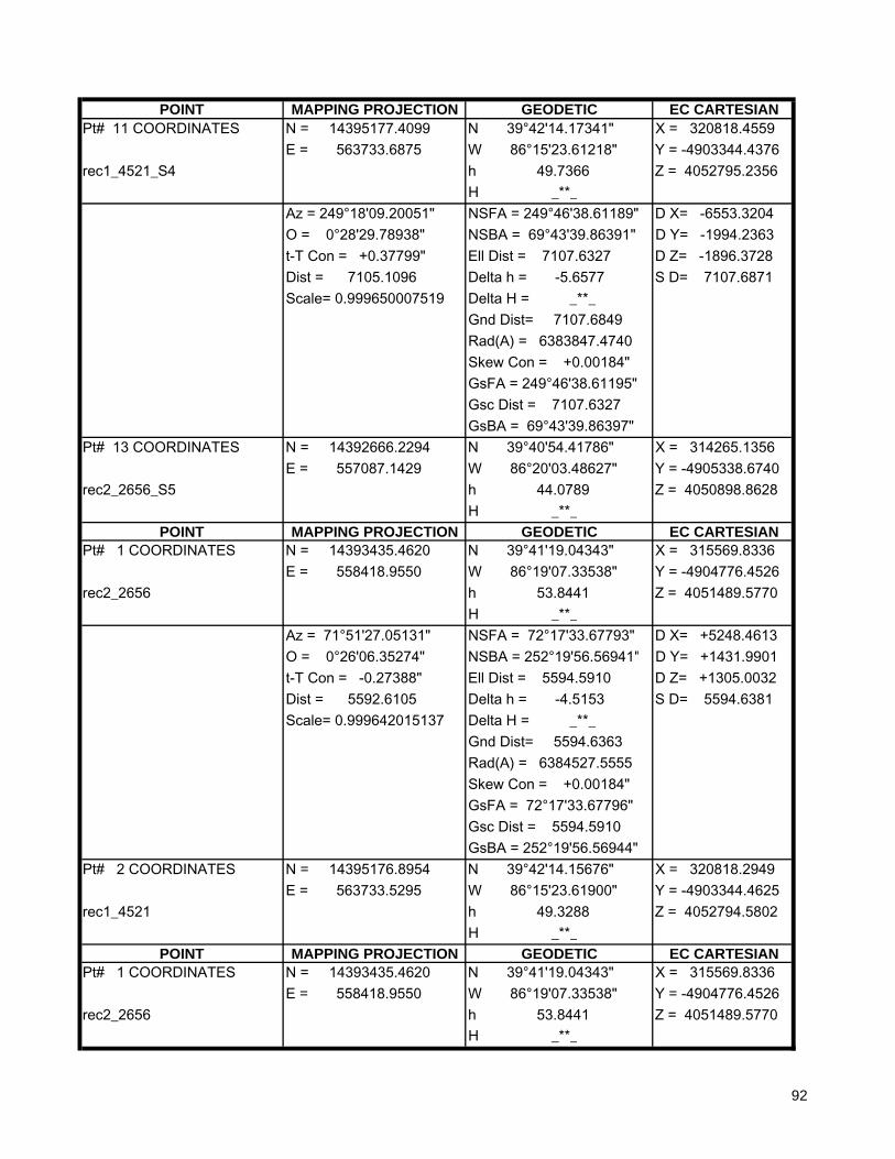
POINT MAPPING PROJECTION GEODETIC EC CARTESIANPt# 11 COORDINATES N = 14395177.4099 N 39°42'14.17341" X = 320818.4559 E = 563733.6875 W 86°15'23.61218" Y = -4903344.4376rec1_4521_S4 h 49.7366 Z = 4052795.2356 H _**_ Az = 249°18'09.20051" NSFA = 249°46'38.61189" D X= -6553.3204 O = 0°28'29.78938" NSBA = 69°43'39.86391" D Y= -1994.2363 t-T Con = +0.37799" Ell Dist = 7107.6327 D Z= -1896.3728 Dist = 7105.1096 Delta h = -5.6577 S D= 7107.6871 Scale= 0.999650007519 Delta H = _**_ Gnd Dist= 7107.6849 Rad(A) = 6383847.4740 Skew Con = +0.00184" GsFA = 249°46'38.61195" Gsc Dist = 7107.6327 GsBA = 69°43'39.86397" Pt# 13 COORDINATES N = 14392666.2294 N 39°40'54.41786" X = 314265.1356 E = 557087.1429 W 86°20'03.48627" Y = -4905338.6740rec2_2656_S5 h 44.0789 Z = 4050898.8628 H _**_

POINT MAPPING PROJECTION GEODETIC EC CARTESIANPt# 1 COORDINATES N = 14393435.4620 N 39°41'19.04343" X = 315569.8336 E = 558418.9550 W 86°19'07.33538" Y = -4904776.4526rec2_2656 h 53.8441 Z = 4051489.5770 H _**_ Az = 71°51'27.05131" NSFA = 72°17'33.67793" D X= +5248.4613 O = 0°26'06.35274" NSBA = 252°19'56.56941" D Y= +1431.9901 t-T Con = -0.27388" Ell Dist = 5594.5910 D Z= +1305.0032 Dist = 5592.6105 Delta h = -4.5153 S D= 5594.6381 Scale= 0.999642015137 Delta H = _**_ Gnd Dist= 5594.6363 Rad(A) = 6384527.5555 Skew Con = +0.00184" GsFA = 72°17'33.67796" Gsc Dist = 5594.5910 GsBA = 252°19'56.56944" Pt# 2 COORDINATES N = 14395176.8954 N 39°42'14.15676" X = 320818.2949 E = 563733.5295 W 86°15'23.61900" Y = -4903344.4625rec1_4521 h 49.3288 Z = 4052794.5802 H _**_

POINT MAPPING PROJECTION GEODETIC EC CARTESIANPt# 1 COORDINATES N = 14393435.4620 N 39°41'19.04343" X = 315569.8336 E = 558418.9550 W 86°19'07.33538" Y = -4904776.4526rec2_2656 h 53.8441 Z = 4051489.5770 H _**_

92

Az = 9°52'54.24423" NSFA = 10°19'01.85302" D X= +1170.8191 O = 0°26'06.35274" NSBA = 190°19'42.54316" D Y= +5404.4255 t-T Con = -1.25605" Ell Dist = 8461.2662 D Z= +6404.3462 Dist = 8458.2467 Delta h = +3.1199 S D= 8461.3404 Scale= 0.999642015137 Delta H = _**_ Gnd Dist= 8461.3396 Rad(A) = 6362307.1015 Skew Con = +0.00129" GsFA = 10°19'01.85306" Gsc Dist = 8461.2662 GsBA = 190°19'42.54321" Pt# 4 COORDINATES N = 14401768.2228 N 39°45'48.94867" X = 316740.6527 E = 559870.5178 W 86°18'03.66945" Y = -4899372.0271rec1_4521_S2 h 56.9641 Z = 4057893.9231 H _**_

POINT MAPPING PROJECTION GEODETIC EC CARTESIANPt# 1 COORDINATES N = 14393435.4620 N 39°41'19.04343" X = 315569.8336 E = 558418.9550 W 86°19'07.33538" Y = -4904776.4526rec2_2656 h 53.8441 Z = 4051489.5770 H _**_ Az = 150°30'41.44226" NSFA = 150°56'47.78883" D X= +24.8834 O = 0°26'06.35274" NSBA = 330°56'48.41095" D Y= -25.2142 t-T Con = +0.00617" Ell Dist = 47.8001 D Z= -32.0930 Dist = 47.7830 Delta h = +0.0975 S D= 47.8006 Scale= 0.999642015137 Delta H = _**_ Gnd Dist= 47.8005 Rad(A) = 6367465.1573 Skew Con = -0.00294" GsFA = 150°56'47.78883" Gsc Dist = 47.8001 GsBA = 330°56'48.41095" Pt# 0 COORDINATES N = 14393393.8690 N 39°41'17.68858" X = 315594.7170 E = 558442.4761 W 86°19'06.36120" Y = -4904801.6668rec3_1947 h 53.9417 Z = 4051457.4840 H _**_

POINT MAPPING PROJECTION GEODETIC EC CARTESIANPt# 1 COORDINATES N = 14393435.4620 N 39°41'19.04343" X = 315569.8336 E = 558418.9550 W 86°19'07.33538" Y = -4904776.4526rec2_2656 h 53.8441 Z = 4051489.5770 H _**_ Az = 271°10'03.11578" NSFA = 271°36'09.49152" D X= -8413.4551 O = 0°26'06.35274" NSBA = 91°32'23.78568" D Y= -390.4933 t-T Con = -0.02300" Ell Dist = 8424.3863 D Z= +181.2720 Dist = 8421.3225 Delta h = +5.4967 S D= 8424.4627 Scale= 0.999642015137 Delta H = _**_

93

Gnd Dist= 8424.4610 Rad(A) = 6386864.8513 Skew Con = -0.00021" GsFA = 271°36'09.49151" Gsc Dist = 8424.3863 GsBA = 91°32'23.78568" Pt# 6 COORDINATES N = 14393607.0537 N 39°41'26.53345" X = 307156.3785 E = 549999.3808 W 86°25'00.75776" Y = -4905166.9459rec3_1947_S1 h 59.3408 Z = 4051670.8490 H _**_

POINT MAPPING PROJECTION GEODETIC EC CARTESIANPt# 1 COORDINATES N = 14393435.4620 N 39°41'19.04343" X = 315569.8336 E = 558418.9550 W 86°19'07.33538" Y = -4904776.4526rec2_2656 h 53.8441 Z = 4051489.5770 H _**_ Az = 158°00'27.51596" NSFA = 158°26'33.86071" D X= +23.5134 O = 0°26'06.35274" NSBA = 338°26'34.43267" D Y= -33.0729 t-T Con = +0.00798" Ell Dist = 58.0821 D Z= -41.5559 Dist = 58.0613 Delta h = +0.0218 S D= 58.0826 Scale= 0.999642015137 Delta H = _**_ Gnd Dist= 58.0826 Rad(A) = 6364911.7160 Skew Con = -0.00237" GsFA = 158°26'33.86071" Gsc Dist = 58.0821 GsBA = 338°26'34.43267" Pt# 3 COORDINATES N = 14393381.6256 N 39°41'17.29190" X = 315593.3470 E = 558440.6980 W 86°19'06.43975" Y = -4904809.5255rec4_2341_S1 h 53.8659 Z = 4051448.0211 H _**_

POINT MAPPING PROJECTION GEODETIC EC CARTESIANPt# 1 COORDINATES N = 14393435.4620 N 39°41'19.04343" X = 315569.8336 E = 558418.9550 W 86°19'07.33538" Y = -4904776.4526rec2_2656 h 53.8441 Z = 4051489.5770 H _**_ Az = 204°34'53.67377" NSFA = 205°00'58.92531" D X= -3278.0801 O = 0°26'06.35274" NSBA = 24°59'22.60435" D Y= -5120.9844 t-T Con = +1.10120" Ell Dist = 8513.3558 D Z= -5958.9160 Dist = 8510.2876 Delta h = -29.1248 S D= 8513.4582 Scale= 0.999642015137 Delta H = _**_ Gnd Dist= 8513.4083 Rad(A) = 6366021.2104 Skew Con = +0.00122" GsFA = 205°00'58.92540" Gsc Dist = 8513.3558

94

GsBA = 24°59'22.60444" Pt# 5 COORDINATES N = 14385696.4629 N 39°37'08.87386" X = 312291.7535 E = 554878.7732 W 86°21'38.27131" Y = -4909897.4370rec4_2341_S4 h 24.7194 Z = 4045530.6610 H _**_

POINT MAPPING PROJECTION GEODETIC EC CARTESIANPt# 9 COORDINATES N = 14392666.2252 N 39°40'54.41772" X = 314265.1373 E = 557087.1444 W 86°20'03.48620" Y = -4905338.6772rec2_2656_S3 h 44.0797 Z = 4050898.8602 H _**_ Az = 17°00'12.48728" NSFA = 17°25'44.11985" D X= +2475.5088 O = 0°25'30.27082" NSBA = 197°27'00.69173" D Y= +5966.6299 t-T Con = -1.36175" Ell Dist = 9521.4741 D Z= +6995.0882 Dist = 9518.0673 Delta h = +12.9157 S D= 9521.5584 Scale= 0.999640121339 Delta H = _**_ Gnd Dist= 9521.5495 Rad(A) = 6363758.2830 Skew Con = +0.00209" GsFA = 17°25'44.11994" Gsc Dist = 9521.4741 GsBA = 197°27'00.69182" Pt# 8 COORDINATES N = 14401768.2295 N 39°45'48.94889" X = 316740.6462 E = 559870.5099 W 86°18'03.66978" Y = -4899372.0473rec1_4521_S3 h 56.9954 Z = 4057893.9484 H _**_


95

POINT MAPPING PROJECTION GEODETIC EC CARTESIANPt# 9 COORDINATES N = 14392666.2252 N 39°40'54.41772" X = 314265.1373 E = 557087.1444 W 86°20'03.48620" Y = -4905338.6772rec2_2656_S3 h 44.0797 Z = 4050898.8602 H _**_ Az = 277°33'40.45785" NSFA = 277°59'10.85371" D X= -7108.7726 O = 0°25'30.27082" NSBA = 97°56'01.02045" D Y= +171.7159 t-T Con = -0.12504" Ell Dist = 7152.5564 D Z= +772.0048 Dist = 7149.9485 Delta h = +15.2825 S D= 7152.6306 Scale= 0.999640121339 Delta H = _**_ Gnd Dist= 7152.6144 Rad(A) = 6386390.1627 Skew Con = -0.00105" GsFA = 277°59'10.85369" Gsc Dist = 7152.5564 GsBA = 97°56'01.02043" Pt# 7 COORDINATES N = 14393607.0566 N 39°41'26.53354" X = 307156.3648 E = 549999.3662 W 86°25'00.75838" Y = -4905166.9613rec3_1947_S2 h 59.3622 Z = 4051670.8650 H _**_

POINT MAPPING PROJECTION GEODETIC EC CARTESIANPt# 9 COORDINATES N = 14392666.2252 N 39°40'54.41772" X = 314265.1373 E = 557087.1444 W 86°20'03.48620" Y = -4905338.6772rec2_2656_S3 h 44.0797 Z = 4050898.8602 H _**_ Az = 178°57'48.83474" NSFA = 179°23'19.09645" D X= +3.2463 O = 0°25'30.27082" NSBA = 359°23'19.11445" D Y= -40.1624 t-T Con = +0.00912" Ell Dist = 62.9672 D Z= -48.3878 Dist = 62.9445 Delta h = +0.1092 S D= 62.9677 Scale= 0.999640121339 Delta H = _**_ Gnd Dist= 62.9676 Rad(A) = 6361491.2280 Skew Con = -0.00006" GsFA = 179°23'19.09645" Gsc Dist = 62.9672 GsBA = 359°23'19.11445" Pt# 10 COORDINATES N = 14392603.2910 N 39°40'52.37619" X = 314268.3836 E = 557088.2830 W 86°20'03.45801" Y = -4905378.8396rec3_1947_S3 h 44.1889 Z = 4050850.4724 H _**_

POINT MAPPING PROJECTION GEODETIC EC CARTESIANPt# 9 COORDINATES N = 14392666.2252 N 39°40'54.41772" X = 314265.1373 E = 557087.1444 W 86°20'03.48620" Y = -4905338.6772rec2_2656_S3 h 44.0797 Z = 4050898.8602 H _**_

96

Az = 197°34'50.93921" NSFA = 198°00'20.22614" D X= -1973.3838 O = 0°25'30.27082" NSBA = 17°59'19.74280" D Y= -4558.7598 t-T Con = +0.98389" Ell Dist = 7313.9007 D Z= -5368.1992 Dist = 7311.2578 Delta h = -19.3603 S D= 7313.9659 Scale= 0.999640121339 Delta H = _**_ Gnd Dist= 7313.9402 Rad(A) = 6363905.9877 Skew Con = +0.00094" GsFA = 198°00'20.22619" Gsc Dist = 7313.9007 GsBA = 17°59'19.74286" Pt# 5 COORDINATES N = 14385696.4629 N 39°37'08.87386" X = 312291.7535 E = 554878.7732 W 86°21'38.27131" Y = -4909897.4370rec4_2341_S4 h 24.7194 Z = 4045530.6610 H _**_


POINT MAPPING PROJECTION GEODETIC EC CARTESIANPt# 0 COORDINATES N = 14393393.8690 N 39°41'17.68858" X = 315594.7170 E = 558442.4761 W 86°19'06.36120" Y = -4904801.6668rec3_1947 h 53.9417 Z = 4051457.4840 H _**_ Az = 71°22'36.30634" NSFA = 71°48'43.54931" D X= +5223.5780 O = 0°26'06.96252" NSBA = 251°51'05.81800" D Y= +1457.2043 t-T Con = -0.28046" Ell Dist = 5585.3837 D Z= +1337.0962 Dist = 5583.4065 Delta h = -4.6129 S D= 5585.4308 Scale= 0.999642048981 Delta H = _**_

97

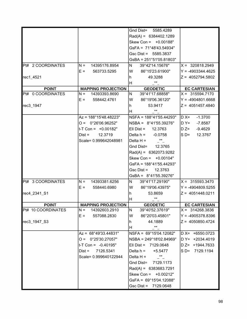
Gnd Dist= 5585.4289 Rad(A) = 6384402.1289 Skew Con = +0.00188" GsFA = 71°48'43.54934" Gsc Dist = 5585.3837 GsBA = 251°51'05.81803" Pt# 2 COORDINATES N = 14395176.8954 N 39°42'14.15676" X = 320818.2949 E = 563733.5295 W 86°15'23.61900" Y = -4903344.4625rec1_4521 h 49.3288 Z = 4052794.5802 H _**_

POINT MAPPING PROJECTION GEODETIC EC CARTESIANPt# 0 COORDINATES N = 14393393.8690 N 39°41'17.68858" X = 315594.7170 E = 558442.4761 W 86°19'06.36120" Y = -4904801.6668rec3_1947 h 53.9417 Z = 4051457.4840 H _**_ Az = 188°15'48.48223" NSFA = 188°41'55.44293" D X= -1.3700 O = 0°26'06.96252" NSBA = 8°41'55.39276" D Y= -7.8587 t-T Con = +0.00182" Ell Dist = 12.3763 D Z= -9.4629 Dist = 12.3719 Delta h = -0.0758 S D= 12.3767 Scale= 0.999642048981 Delta H = _**_ Gnd Dist= 12.3765 Rad(A) = 6362073.9282 Skew Con = +0.00104" GsFA = 188°41'55.44293" Gsc Dist = 12.3763 GsBA = 8°41'55.39276" Pt# 3 COORDINATES N = 14393381.6256 N 39°41'17.29190" X = 315593.3470 E = 558440.6980 W 86°19'06.43975" Y = -4904809.5255rec4_2341_S1 h 53.8659 Z = 4051448.0211 H _**_

POINT MAPPING PROJECTION GEODETIC EC CARTESIANPt# 10 COORDINATES N = 14392603.2910 N 39°40'52.37619" X = 314268.3836 E = 557088.2830 W 86°20'03.45801" Y = -4905378.8396rec3_1947_S3 h 44.1889 Z = 4050850.4724 H _**_ Az = 68°49'33.44831" NSFA = 69°15'04.12082" D X= +6550.0723 O = 0°25'30.27057" NSBA = 249°18'02.84969" D Y= +2034.4019 t-T Con = -0.40195" Ell Dist = 7129.0648 D Z= +1944.7633 Dist = 7126.5341 Delta h = +5.5477 S D= 7129.1194 Scale= 0.999640122944 Delta H = _**_ Gnd Dist= 7129.1173 Rad(A) = 6383683.7291 Skew Con = +0.00212" GsFA = 69°15'04.12088" Gsc Dist = 7129.0648

98

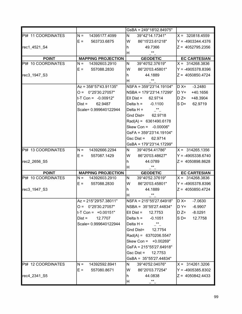
GsBA = 249°18'02.84975" Pt# 11 COORDINATES N = 14395177.4099 N 39°42'14.17341" X = 320818.4559 E = 563733.6875 W 86°15'23.61218" Y = -4903344.4376rec1_4521_S4 h 49.7366 Z = 4052795.2356 H _**_

POINT MAPPING PROJECTION GEODETIC EC CARTESIANPt# 10 COORDINATES N = 14392603.2910 N 39°40'52.37619" X = 314268.3836 E = 557088.2830 W 86°20'03.45801" Y = -4905378.8396rec3_1947_S3 h 44.1889 Z = 4050850.4724 H _**_ Az = 358°57'43.91135" NSFA = 359°23'14.19104" D X= -3.2480 O = 0°25'30.27057" NSBA = 179°23'14.17299" D Y= +40.1656 t-T Con = -0.00912" Ell Dist = 62.9714 D Z= +48.3904 Dist = 62.9487 Delta h = -0.1100 S D= 62.9719 Scale= 0.999640122944 Delta H = _**_ Gnd Dist= 62.9718 Rad(A) = 6361490.6178 Skew Con = -0.00006" GsFA = 359°23'14.19104" Gsc Dist = 62.9714 GsBA = 179°23'14.17299" Pt# 13 COORDINATES N = 14392666.2294 N 39°40'54.41786" X = 314265.1356 E = 557087.1429 W 86°20'03.48627" Y = -4905338.6740rec2_2656_S5 h 44.0789 Z = 4050898.8628 H _**_

POINT MAPPING PROJECTION GEODETIC EC CARTESIANPt# 10 COORDINATES N = 14392603.2910 N 39°40'52.37619" X = 314268.3836 E = 557088.2830 W 86°20'03.45801" Y = -4905378.8396rec3_1947_S3 h 44.1889 Z = 4050850.4724 H _**_ Az = 215°29'57.38011" NSFA = 215°55'27.64918" D X= -7.0630 O = 0°25'30.27057" NSBA = 35°55'27.44834" D Y= -6.9907 t-T Con = +0.00151" Ell Dist = 12.7753 D Z= -8.0291 Dist = 12.7707 Delta h = -0.1051 S D= 12.7758 Scale= 0.999640122944 Delta H = _**_ Gnd Dist= 12.7754 Rad(A) = 6370206.5547 Skew Con = +0.00269" GsFA = 215°55'27.64918" Gsc Dist = 12.7753 GsBA = 35°55'27.44834" Pt# 12 COORDINATES N = 14392592.8941 N 39°40'52.04076" X = 314261.3206 E = 557080.8671 W 86°20'03.77254" Y = -4905385.8302rec4_2341_S5 h 44.0838 Z = 4050842.4433 H _**_

99



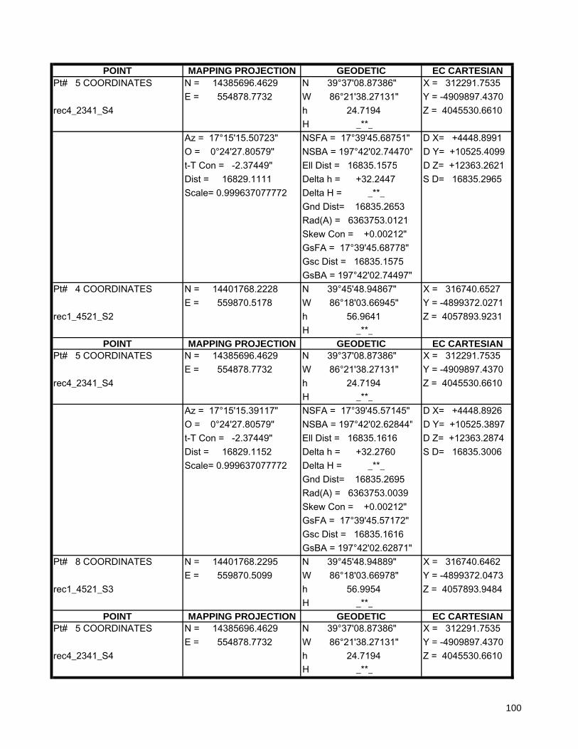
POINT MAPPING PROJECTION GEODETIC EC CARTESIANPt# 5 COORDINATES N = 14385696.4629 N 39°37'08.87386" X = 312291.7535 E = 554878.7732 W 86°21'38.27131" Y = -4909897.4370rec4_2341_S4 h 24.7194 Z = 4045530.6610 H _**_

100

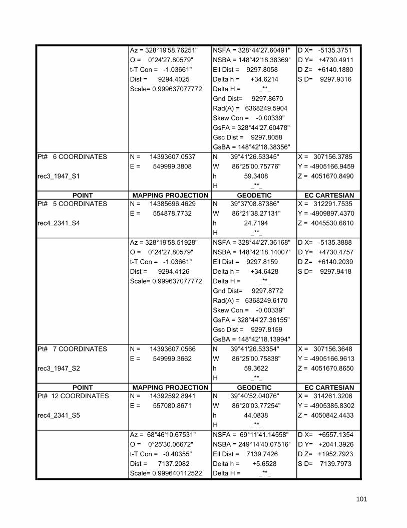
Az = 328°19'58.76251" NSFA = 328°44'27.60491" D X= -5135.3751 O = 0°24'27.80579" NSBA = 148°42'18.38369" D Y= +4730.4911 t-T Con = -1.03661" Ell Dist = 9297.8058 D Z= +6140.1880 Dist = 9294.4025 Delta h = +34.6214 S D= 9297.9316 Scale= 0.999637077772 Delta H = _**_ Gnd Dist= 9297.8670 Rad(A) = 6368249.5904 Skew Con = -0.00339" GsFA = 328°44'27.60478" Gsc Dist = 9297.8058 GsBA = 148°42'18.38356" Pt# 6 COORDINATES N = 14393607.0537 N 39°41'26.53345" X = 307156.3785 E = 549999.3808 W 86°25'00.75776" Y = -4905166.9459rec3_1947_S1 h 59.3408 Z = 4051670.8490 H _**_

POINT MAPPING PROJECTION GEODETIC EC CARTESIANPt# 5 COORDINATES N = 14385696.4629 N 39°37'08.87386" X = 312291.7535 E = 554878.7732 W 86°21'38.27131" Y = -4909897.4370rec4_2341_S4 h 24.7194 Z = 4045530.6610 H _**_ Az = 328°19'58.51928" NSFA = 328°44'27.36168" D X= -5135.3888 O = 0°24'27.80579" NSBA = 148°42'18.14007" D Y= +4730.4757 t-T Con = -1.03661" Ell Dist = 9297.8159 D Z= +6140.2039 Dist = 9294.4126 Delta h = +34.6428 S D= 9297.9418 Scale= 0.999637077772 Delta H = _**_ Gnd Dist= 9297.8772 Rad(A) = 6368249.6170 Skew Con = -0.00339" GsFA = 328°44'27.36155" Gsc Dist = 9297.8159 GsBA = 148°42'18.13994" Pt# 7 COORDINATES N = 14393607.0566 N 39°41'26.53354" X = 307156.3648 E = 549999.3662 W 86°25'00.75838" Y = -4905166.9613rec3_1947_S2 h 59.3622 Z = 4051670.8650 H _**_

POINT MAPPING PROJECTION GEODETIC EC CARTESIANPt# 12 COORDINATES N = 14392592.8941 N 39°40'52.04076" X = 314261.3206 E = 557080.8671 W 86°20'03.77254" Y = -4905385.8302rec4_2341_S5 h 44.0838 Z = 4050842.4433 H _**_ Az = 68°46'10.67531" NSFA = 69°11'41.14558" D X= +6557.1354 O = 0°25'30.06672" NSBA = 249°14'40.07516" D Y= +2041.3926 t-T Con = -0.40355" Ell Dist = 7139.7426 D Z= +1952.7923 Dist = 7137.2082 Delta h = +5.6528 S D= 7139.7973 Scale= 0.999640112522 Delta H = _**_

101

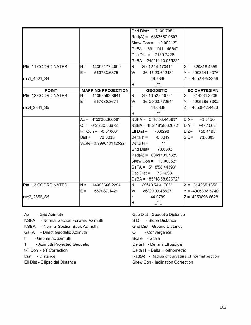
Gnd Dist= 7139.7951 Rad(A) = 6383667.0607 Skew Con = +0.00212" GsFA = 69°11'41.14564" Gsc Dist = 7139.7426 GsBA = 249°14'40.07522" Pt# 11 COORDINATES N = 14395177.4099 N 39°42'14.17341" X = 320818.4559 E = 563733.6875 W 86°15'23.61218" Y = -4903344.4376rec1_4521_S4 h 49.7366 Z = 4052795.2356 H _**_

POINT MAPPING PROJECTION GEODETIC EC CARTESIANPt# 12 COORDINATES N = 14392592.8941 N 39°40'52.04076" X = 314261.3206 E = 557080.8671 W 86°20'03.77254" Y = -4905385.8302rec4_2341_S5 h 44.0838 Z = 4050842.4433 H _**_ Az = 4°53'28.36658" NSFA = 5°18'58.44393" D X= +3.8150 O = 0°25'30.06672" NSBA = 185°18'58.62672" D Y= +47.1563 t-T Con = -0.01063" Ell Dist = 73.6298 D Z= +56.4195 Dist = 73.6033 Delta h = -0.0049 S D= 73.6303 Scale= 0.999640112522 Delta H = _**_ Gnd Dist= 73.6303 Rad(A) = 6361704.7625 Skew Con = +0.00052" GsFA = 5°18'58.44393" Gsc Dist = 73.6298 GsBA = 185°18'58.62672" Pt# 13 COORDINATES N = 14392666.2294 N 39°40'54.41786" X = 314265.1356 E = 557087.1429 W 86°20'03.48627" Y = -4905338.6740rec2_2656_S5 h 44.0789 Z = 4050898.8628 H _**_

Az - Grid Azimuth Gsc Dist - Geodetic Distance NSFA - Normal Section Forward Azimuth S D - Slope Distance NSBA - Normal Section Back Azimuth Gnd Dist - Ground Distance GsFA - Direct Geodetic Azimuth O - Convergence t - Geometric azimuth Scale - Scale T - Azimuth Projected Geodetic Delta h - Delta h Ellipsoidal t-T Con - t-T Correction Delta H - Delta H orthometric Dist - Distance Rad(A) - Radius of curvature of normal section Ell Dist - Ellipsoidal Distance Skew Con - Inclination Correction

102

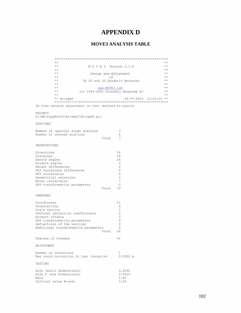
102

APPENDIX D

MOVE3 ANALYSIS TABLE ************************************************************ ** ** ** M O V E 3 Version 3.1.0 ** ** ** ** Design and Adjustment ** ** of ** ** 3D 2D and 1D Geodetic Networks ** ** ** ** www.MOVE3.com ** ** (c) 1993-2001 Grontmij Geogroep bv ** ** ** ** BridgeP 06-07-2003 21:21:12 ** ************************************************************ 3D free network adjustment on User defined ellipsoid PROJECT R:\RA\CopyMove3\Bridge3\BridgeP.prj STATIONS Number of (partly) known stations 3 Number of unknown stations 4 Total 7 OBSERVATIONS Directions 24 Distances 24 Zenith angles 24 Azimuth angles 0 Height differences 0 GPS coordinate differences 0 GPS coordinates 0 Geometrical relations 0 Known coordinates 7 GPS transformation parameters 0 Total 79 UNKNOWNS Coordinates 21 Orientations 4 Scale factors 1 Vertical refraction coefficients 0 Azimuth offsets 0 GPS transformation parameters 0 Deflections of the vertical 0 Additional transformation parameters 2 Total 28 Degrees of freedom 51 ADJUSTMENT Number of iterations 1 Max coord correction in last iteration 0.0000 m TESTING Alfa (multi dimensional) 0.2642 Alfa 0 (one dimensional) 0.0010 Beta 0.80 Critical value W-test 3.29

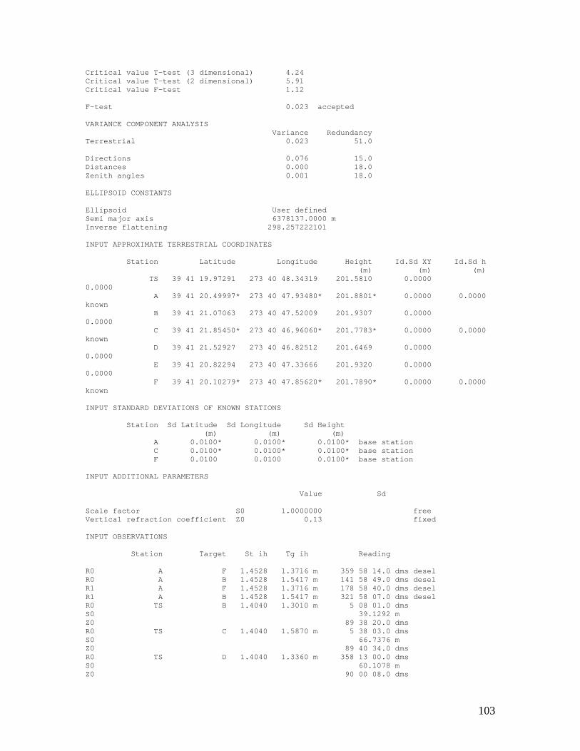
103

Critical value T-test (3 dimensional) 4.24 Critical value T-test (2 dimensional) 5.91 Critical value F-test 1.12 F-test 0.023 accepted VARIANCE COMPONENT ANALYSIS Variance Redundancy Terrestrial 0.023 51.0 Directions 0.076 15.0 Distances 0.000 18.0 Zenith angles 0.001 18.0 ELLIPSOID CONSTANTS Ellipsoid User defined Semi major axis 6378137.0000 m Inverse flattening 298.257222101 INPUT APPROXIMATE TERRESTRIAL COORDINATES Station Latitude Longitude Height Id.Sd XY Id.Sd h (m) (m) (m) TS 39 41 19.97291 273 40 48.34319 201.5810 0.0000 0.0000 A 39 41 20.49997* 273 40 47.93480* 201.8801* 0.0000 0.0000 known B 39 41 21.07063 273 40 47.52009 201.9307 0.0000 0.0000 C 39 41 21.85450* 273 40 46.96060* 201.7783* 0.0000 0.0000 known D 39 41 21.52927 273 40 46.82512 201.6469 0.0000 0.0000 E 39 41 20.82294 273 40 47.33666 201.9320 0.0000 0.0000 F 39 41 20.10279* 273 40 47.85620* 201.7890* 0.0000 0.0000 known INPUT STANDARD DEVIATIONS OF KNOWN STATIONS Station Sd Latitude Sd Longitude Sd Height (m) (m) (m) A 0.0100* 0.0100* 0.0100* base station C 0.0100* 0.0100* 0.0100* base station F 0.0100 0.0100 0.0100* base station INPUT ADDITIONAL PARAMETERS Value Sd Scale factor S0 1.0000000 free Vertical refraction coefficient Z0 0.13 fixed INPUT OBSERVATIONS Station Target St ih Tg ih Reading R0 A F 1.4528 1.3716 m 359 58 14.0 dms desel R0 A B 1.4528 1.5417 m 141 58 49.0 dms desel R1 A F 1.4528 1.3716 m 178 58 40.0 dms desel R1 A B 1.4528 1.5417 m 321 58 07.0 dms desel R0 TS B 1.4040 1.3010 m 5 08 01.0 dms S0 39.1292 m Z0 89 38 20.0 dms R0 TS C 1.4040 1.5870 m 5 38 03.0 dms S0 66.7376 m Z0 89 40 34.0 dms R0 TS D 1.4040 1.3360 m 358 13 00.0 dms S0 60.1078 m Z0 90 00 08.0 dms

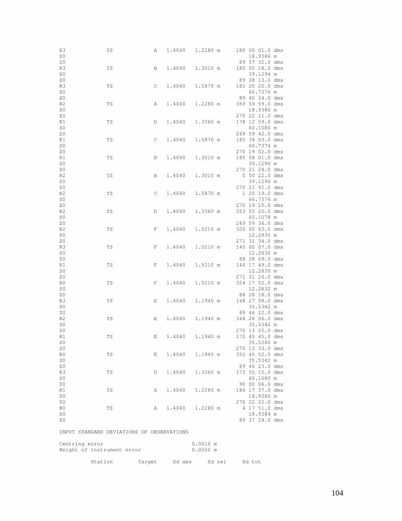
104

R3 TS A 1.4040 1.2280 m 180 00 01.0 dms S0 18.9386 m Z0 89 37 32.0 dms R3 TS B 1.4040 1.3010 m 180 50 18.0 dms S0 39.1294 m Z0 89 38 13.0 dms R3 TS C 1.4040 1.5870 m 181 20 20.0 dms S0 66.7376 m Z0 89 40 34.0 dms R2 TS A 1.4040 1.2280 m 359 59 59.0 dms S0 18.9386 m Z0 270 22 11.0 dms R1 TS D 1.4040 1.3360 m 178 12 59.0 dms S0 60.1080 m Z0 269 59 42.0 dms R1 TS C 1.4040 1.5870 m 185 38 03.0 dms S0 66.7374 m Z0 270 19 02.0 dms R1 TS B 1.4040 1.3010 m 185 08 01.0 dms S0 39.1296 m Z0 270 21 24.0 dms R2 TS B 1.4040 1.3010 m 0 50 22.0 dms S0 39.1296 m Z0 270 21 41.0 dms R2 TS C 1.4040 1.5870 m 1 20 19.0 dms S0 66.7376 m Z0 270 19 15.0 dms R2 TS D 1.4040 1.3360 m 353 55 20.0 dms S0 60.1078 m Z0 269 59 36.0 dms R2 TS F 1.4040 1.5210 m 320 00 03.0 dms S0 12.2830 m Z0 271 31 34.0 dms R3 TS F 1.4040 1.5210 m 140 00 07.0 dms S0 12.2830 m Z0 88 28 09.0 dms R1 TS F 1.4040 1.5210 m 144 17 49.0 dms S0 12.2830 m Z0 271 31 26.0 dms R0 TS F 1.4040 1.5210 m 324 17 52.0 dms S0 12.2832 m Z0 88 28 18.0 dms R3 TS E 1.4040 1.1940 m 168 27 58.0 dms S0 35.5342 m Z0 89 46 22.0 dms R2 TS E 1.4040 1.1940 m 348 28 06.0 dms S0 35.5342 m Z0 270 13 25.0 dms R1 TS E 1.4040 1.1940 m 172 45 45.0 dms S0 35.5340 m Z0 270 13 33.0 dms R0 TS E 1.4040 1.1940 m 352 45 52.0 dms S0 35.5342 m Z0 89 46 23.0 dms R3 TS D 1.4040 1.3360 m 173 55 15.0 dms S0 60.1080 m Z0 90 00 06.0 dms R1 TS A 1.4040 1.2280 m 184 17 37.0 dms S0 18.9386 m Z0 270 22 22.0 dms R0 TS A 1.4040 1.2280 m 4 17 51.0 dms S0 18.9384 m Z0 89 37 24.0 dms INPUT STANDARD DEVIATIONS OF OBSERVATIONS Centring error 0.0010 m Height of instrument error 0.0500 m Station Target Sd abs Sd rel Sd tot

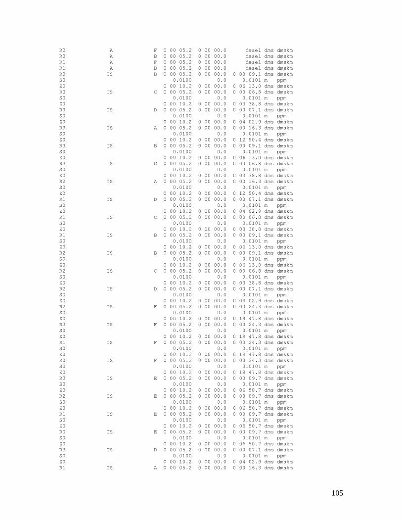
105

R0 A F 0 00 05.2 0 00 00.0 desel dms dmskm R0 A B 0 00 05.2 0 00 00.0 desel dms dmskm R1 A F 0 00 05.2 0 00 00.0 desel dms dmskm R1 A B 0 00 05.2 0 00 00.0 desel dms dmskm R0 TS B 0 00 05.2 0 00 00.0 0 00 09.1 dms dmskm S0 0.0100 0.0 0.0101 m ppm Z0 0 00 10.2 0 00 00.0 0 06 13.0 dms dmskm R0 TS C 0 00 05.2 0 00 00.0 0 00 06.8 dms dmskm S0 0.0100 0.0 0.0101 m ppm Z0 0 00 10.2 0 00 00.0 0 03 38.8 dms dmskm R0 TS D 0 00 05.2 0 00 00.0 0 00 07.1 dms dmskm S0 0.0100 0.0 0.0101 m ppm Z0 0 00 10.2 0 00 00.0 0 04 02.9 dms dmskm R3 TS A 0 00 05.2 0 00 00.0 0 00 16.3 dms dmskm S0 0.0100 0.0 0.0101 m ppm Z0 0 00 10.2 0 00 00.0 0 12 50.4 dms dmskm R3 TS B 0 00 05.2 0 00 00.0 0 00 09.1 dms dmskm S0 0.0100 0.0 0.0101 m ppm Z0 0 00 10.2 0 00 00.0 0 06 13.0 dms dmskm R3 TS C 0 00 05.2 0 00 00.0 0 00 06.8 dms dmskm S0 0.0100 0.0 0.0101 m ppm Z0 0 00 10.2 0 00 00.0 0 03 38.8 dms dmskm R2 TS A 0 00 05.2 0 00 00.0 0 00 16.3 dms dmskm S0 0.0100 0.0 0.0101 m ppm Z0 0 00 10.2 0 00 00.0 0 12 50.4 dms dmskm R1 TS D 0 00 05.2 0 00 00.0 0 00 07.1 dms dmskm S0 0.0100 0.0 0.0101 m ppm Z0 0 00 10.2 0 00 00.0 0 04 02.9 dms dmskm R1 TS C 0 00 05.2 0 00 00.0 0 00 06.8 dms dmskm S0 0.0100 0.0 0.0101 m ppm Z0 0 00 10.2 0 00 00.0 0 03 38.8 dms dmskm R1 TS B 0 00 05.2 0 00 00.0 0 00 09.1 dms dmskm S0 0.0100 0.0 0.0101 m ppm Z0 0 00 10.2 0 00 00.0 0 06 13.0 dms dmskm R2 TS B 0 00 05.2 0 00 00.0 0 00 09.1 dms dmskm S0 0.0100 0.0 0.0101 m ppm Z0 0 00 10.2 0 00 00.0 0 06 13.0 dms dmskm R2 TS C 0 00 05.2 0 00 00.0 0 00 06.8 dms dmskm S0 0.0100 0.0 0.0101 m ppm Z0 0 00 10.2 0 00 00.0 0 03 38.8 dms dmskm R2 TS D 0 00 05.2 0 00 00.0 0 00 07.1 dms dmskm S0 0.0100 0.0 0.0101 m ppm Z0 0 00 10.2 0 00 00.0 0 04 02.9 dms dmskm R2 TS F 0 00 05.2 0 00 00.0 0 00 24.3 dms dmskm S0 0.0100 0.0 0.0101 m ppm Z0 0 00 10.2 0 00 00.0 0 19 47.8 dms dmskm R3 TS F 0 00 05.2 0 00 00.0 0 00 24.3 dms dmskm S0 0.0100 0.0 0.0101 m ppm Z0 0 00 10.2 0 00 00.0 0 19 47.8 dms dmskm R1 TS F 0 00 05.2 0 00 00.0 0 00 24.3 dms dmskm S0 0.0100 0.0 0.0101 m ppm Z0 0 00 10.2 0 00 00.0 0 19 47.8 dms dmskm R0 TS F 0 00 05.2 0 00 00.0 0 00 24.3 dms dmskm S0 0.0100 0.0 0.0101 m ppm Z0 0 00 10.2 0 00 00.0 0 19 47.8 dms dmskm R3 TS E 0 00 05.2 0 00 00.0 0 00 09.7 dms dmskm S0 0.0100 0.0 0.0101 m ppm Z0 0 00 10.2 0 00 00.0 0 06 50.7 dms dmskm R2 TS E 0 00 05.2 0 00 00.0 0 00 09.7 dms dmskm S0 0.0100 0.0 0.0101 m ppm Z0 0 00 10.2 0 00 00.0 0 06 50.7 dms dmskm R1 TS E 0 00 05.2 0 00 00.0 0 00 09.7 dms dmskm S0 0.0100 0.0 0.0101 m ppm Z0 0 00 10.2 0 00 00.0 0 06 50.7 dms dmskm R0 TS E 0 00 05.2 0 00 00.0 0 00 09.7 dms dmskm S0 0.0100 0.0 0.0101 m ppm Z0 0 00 10.2 0 00 00.0 0 06 50.7 dms dmskm R3 TS D 0 00 05.2 0 00 00.0 0 00 07.1 dms dmskm S0 0.0100 0.0 0.0101 m ppm Z0 0 00 10.2 0 00 00.0 0 04 02.9 dms dmskm R1 TS A 0 00 05.2 0 00 00.0 0 00 16.3 dms dmskm

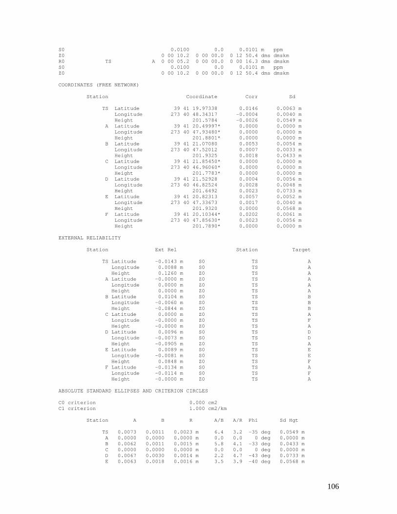
106

S0 0.0100 0.0 0.0101 m ppm Z0 0 00 10.2 0 00 00.0 0 12 50.4 dms dmskm R0 TS A 0 00 05.2 0 00 00.0 0 00 16.3 dms dmskm S0 0.0100 0.0 0.0101 m ppm Z0 0 00 10.2 0 00 00.0 0 12 50.4 dms dmskm COORDINATES (FREE NETWORK) Station Coordinate Corr Sd TS Latitude 39 41 19.97338 0.0146 0.0063 m Longitude 273 40 48.34317 -0.0004 0.0040 m Height 201.5784 -0.0026 0.0549 m A Latitude 39 41 20.49997* 0.0000 0.0000 m Longitude 273 40 47.93480* 0.0000 0.0000 m Height 201.8801* 0.0000 0.0000 m B Latitude 39 41 21.07080 0.0053 0.0054 m Longitude 273 40 47.52012 0.0007 0.0033 m Height 201.9325 0.0018 0.0433 m C Latitude 39 41 21.85450* 0.0000 0.0000 m Longitude 273 40 46.96060* 0.0000 0.0000 m Height 201.7783* 0.0000 0.0000 m D Latitude 39 41 21.52928 0.0004 0.0056 m Longitude 273 40 46.82524 0.0028 0.0048 m Height 201.6492 0.0023 0.0733 m E Latitude 39 41 20.82313 0.0057 0.0052 m Longitude 273 40 47.33673 0.0017 0.0040 m Height 201.9320 0.0000 0.0568 m F Latitude 39 41 20.10344* 0.0202 0.0061 m Longitude 273 40 47.85630* 0.0023 0.0056 m Height 201.7890* 0.0000 0.0000 m EXTERNAL RELIABILITY Station Ext Rel Station Target TS Latitude -0.0143 m S0 TS A Longitude 0.0088 m S0 TS A Height 0.1260 m Z0 TS A A Latitude -0.0000 m Z0 TS A Longitude 0.0000 m Z0 TS A Height 0.0000 m Z0 TS A B Latitude 0.0104 m S0 TS B Longitude -0.0060 m S0 TS B Height -0.0844 m Z0 TS B C Latitude 0.0000 m Z0 TS A Longitude -0.0000 m Z0 TS F Height -0.0000 m Z0 TS A D Latitude 0.0096 m S0 TS D Longitude -0.0073 m S0 TS D Height -0.0905 m Z0 TS A E Latitude 0.0089 m S0 TS E Longitude -0.0081 m S0 TS E Height 0.0848 m Z0 TS F F Latitude -0.0134 m S0 TS A Longitude -0.0114 m S0 TS F Height -0.0000 m Z0 TS A ABSOLUTE STANDARD ELLIPSES AND CRITERION CIRCLES C0 criterion 0.000 cm2 C1 criterion 1.000 cm2/km Station A B R A/B A/R Phi Sd Hgt TS 0.0073 0.0011 0.0023 m 6.4 3.2 -35 deg 0.0549 m A 0.0000 0.0000 0.0000 m 0.0 0.0 0 deg 0.0000 m B 0.0062 0.0011 0.0015 m 5.8 4.1 -33 deg 0.0433 m C 0.0000 0.0000 0.0000 m 0.0 0.0 0 deg 0.0000 m D 0.0067 0.0030 0.0014 m 2.2 4.7 -43 deg 0.0733 m E 0.0063 0.0018 0.0016 m 3.5 3.9 -40 deg 0.0568 m

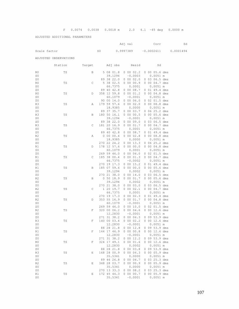
107

F 0.0074 0.0038 0.0018 m 2.0 4.1 -45 deg 0.0000 m ADJUSTED ADDITIONAL PARAMETERS Adj val Corr Sd Scale factor S0 0.9997389 -0.0002611 0.0001494 ADJUSTED OBSERVATIONS Station Target Adj obs Resid Sd R0 TS B 5 08 01.8 0 00 02.2 0 00 05.6 dms S0 39.1294 -0.0003 0.0051 m Z0 89 38 22.0 0 00 02.0 0 03 06.5 dms R0 TS C 5 38 02.5 0 00 00.9 0 00 04.7 dms S0 66.7375 0.0001 0.0051 m Z0 89 40 42.8 0 00 08.7 0 01 49.4 dms R0 TS D 358 12 59.8 0 00 01.2 0 00 04.8 dms S0 60.1079 -0.0001 0.0051 m Z0 90 00 14.0 0 00 06.0 0 02 01.5 dms R3 TS A 179 59 57.6 0 00 02.0 0 00 08.8 dms S0 18.9385 0.0000 0.0051 m Z0 89 37 35.7 0 00 03.7 0 06 25.2 dms R3 TS B 180 50 16.1 0 00 00.5 0 00 05.6 dms S0 39.1294 -0.0001 0.0051 m Z0 89 38 22.0 0 00 09.0 0 03 06.5 dms R3 TS C 181 20 16.9 0 00 01.7 0 00 04.7 dms S0 66.7375 0.0001 0.0051 m Z0 89 40 42.8 0 00 08.7 0 01 49.4 dms R2 TS A 0 00 00.4 0 00 02.8 0 00 08.8 dms S0 18.9385 0.0000 0.0051 m Z0 270 22 24.2 0 00 13.3 0 06 25.2 dms R1 TS D 178 12 57.6 0 00 00.0 0 00 04.8 dms S0 60.1079 0.0001 0.0051 m Z0 269 59 46.0 0 00 04.0 0 02 01.5 dms R1 TS C 185 38 00.4 0 00 01.3 0 00 04.7 dms S0 66.7375 -0.0002 0.0051 m Z0 270 19 17.3 0 00 15.2 0 01 49.4 dms R1 TS B 185 07 59.6 0 00 00.0 0 00 05.6 dms S0 39.1294 0.0002 0.0051 m Z0 270 21 38.0 0 00 14.0 0 03 06.5 dms R2 TS B 0 50 18.9 0 00 01.7 0 00 05.6 dms S0 39.1294 0.0002 0.0051 m Z0 270 21 38.0 0 00 03.0 0 03 06.5 dms R2 TS C 1 20 19.7 0 00 02.1 0 00 04.7 dms S0 66.7375 0.0001 0.0051 m Z0 270 19 17.3 0 00 02.3 0 01 49.4 dms R2 TS D 353 55 16.9 0 00 01.7 0 00 04.8 dms S0 60.1079 -0.0001 0.0051 m Z0 269 59 46.0 0 00 10.0 0 02 01.5 dms R2 TS F 320 00 06.2 0 00 04.6 0 00 12.6 dms S0 12.2830 -0.0001 0.0051 m Z0 271 31 38.2 0 00 04.3 0 09 53.9 dms R3 TS F 140 00 03.4 0 00 02.2 0 00 12.6 dms S0 12.2830 -0.0001 0.0051 m Z0 88 28 21.8 0 00 12.8 0 09 53.9 dms R1 TS F 144 17 46.9 0 00 00.8 0 00 12.6 dms S0 12.2830 -0.0001 0.0051 m Z0 271 31 38.2 0 00 12.2 0 09 53.9 dms R0 TS F 324 17 49.1 0 00 01.6 0 00 12.6 dms S0 12.2830 0.0002 0.0051 m Z0 88 28 21.8 0 00 03.8 0 09 53.9 dms R3 TS E 168 28 00.9 0 00 04.3 0 00 05.9 dms S0 35.5341 0.0000 0.0051 m Z0 89 46 26.8 0 00 04.7 0 03 25.3 dms R2 TS E 348 28 03.7 0 00 00.9 0 00 05.9 dms S0 35.5341 0.0000 0.0051 m Z0 270 13 33.3 0 00 08.2 0 03 25.3 dms R1 TS E 172 45 44.3 0 00 00.7 0 00 05.9 dms S0 35.5341 -0.0001 0.0051 m

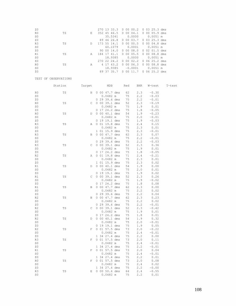
108

Z0 270 13 33.3 0 00 00.2 0 03 25.3 dms R0 TS E 352 45 46.5 0 00 04.1 0 00 05.9 dms S0 35.5341 0.0000 0.0051 m Z0 89 46 26.8 0 00 03.7 0 03 25.3 dms R3 TS D 173 55 14.1 0 00 00.5 0 00 04.8 dms S0 60.1079 0.0001 0.0051 m Z0 90 00 14.0 0 00 08.0 0 02 01.5 dms R1 TS A 184 17 41.1 0 00 05.5 0 00 08.8 dms S0 18.9385 0.0000 0.0051 m Z0 270 22 24.2 0 00 02.2 0 06 25.2 dms R0 TS A 4 17 43.2 0 00 06.3 0 00 08.8 dms S0 18.9385 -0.0001 0.0051 m Z0 89 37 35.7 0 00 11.7 0 06 25.2 dms TEST OF OBSERVATIONS Station Target MDB Red BNR W-test T-test R0 TS B 0 00 47.7 dms 62 2.3 -0.30 S0 0.0482 m 75 2.2 -0.03 Z0 0 29 39.6 dms 75 2.2 -0.01 R0 TS C 0 00 39.1 dms 52 2.3 -0.19 S0 0.0482 m 75 1.9 0.01 Z0 0 17 24.2 dms 75 1.8 -0.05 R0 TS D 0 00 40.1 dms 54 1.9 -0.23 S0 0.0482 m 75 2.0 -0.01 Z0 0 19 19.1 dms 75 1.9 -0.03 R3 TS A 0 01 19.8 dms 71 2.4 0.15 S0 0.0482 m 75 2.3 0.01 Z0 1 01 15.9 dms 75 2.3 -0.01 R3 TS B 0 00 47.7 dms 62 2.3 0.07 S0 0.0482 m 75 2.2 -0.01 Z0 0 29 39.6 dms 75 2.2 -0.03 R3 TS C 0 00 39.1 dms 52 2.3 0.36 S0 0.0482 m 75 1.9 0.01 Z0 0 17 24.2 dms 75 1.8 -0.05 R2 TS A 0 01 19.8 dms 71 2.4 -0.21 S0 0.0482 m 75 2.3 0.01 Z0 1 01 15.9 dms 75 2.3 0.02 R1 TS D 0 00 40.1 dms 54 1.9 0.00 S0 0.0482 m 75 2.0 0.01 Z0 0 19 19.1 dms 75 1.9 0.02 R1 TS C 0 00 39.1 dms 52 2.3 0.26 S0 0.0482 m 75 1.9 -0.02 Z0 0 17 24.2 dms 75 1.8 0.08 R1 TS B 0 00 47.7 dms 62 2.3 0.00 S0 0.0482 m 75 2.2 0.02 Z0 0 29 39.6 dms 75 2.2 0.04 R2 TS B 0 00 47.7 dms 62 2.3 0.23 S0 0.0482 m 75 2.2 0.02 Z0 0 29 39.6 dms 75 2.2 -0.01 R2 TS C 0 00 39.1 dms 52 2.3 -0.42 S0 0.0482 m 75 1.9 0.01 Z0 0 17 24.2 dms 75 1.8 0.01 R2 TS D 0 00 40.1 dms 54 1.9 0.32 S0 0.0482 m 75 2.0 -0.01 Z0 0 19 19.1 dms 75 1.9 0.05 R2 TS F 0 01 57.5 dms 73 2.0 -0.22 S0 0.0482 m 75 2.4 -0.01 Z0 1 34 27.4 dms 75 2.2 0.00 R3 TS F 0 01 57.5 dms 73 2.0 0.11 S0 0.0482 m 75 2.4 -0.01 Z0 1 34 27.4 dms 75 2.2 -0.01 R1 TS F 0 01 57.5 dms 73 2.0 0.04 S0 0.0482 m 75 2.4 -0.01 Z0 1 34 27.4 dms 75 2.2 0.01 R0 TS F 0 01 57.5 dms 73 2.0 0.08 S0 0.0482 m 75 2.4 0.02 Z0 1 34 27.4 dms 75 2.2 -0.00 R3 TS E 0 00 50.4 dms 64 2.4 -0.55 S0 0.0482 m 75 2.2 0.01

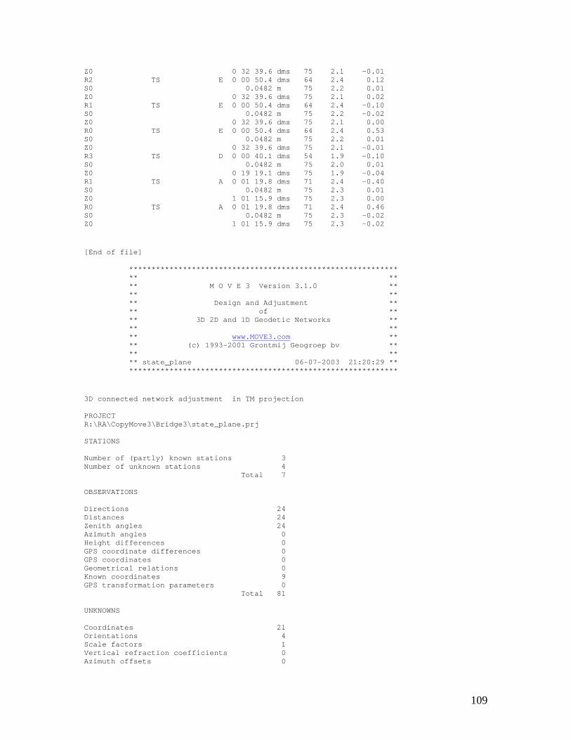
109

Z0 0 32 39.6 dms 75 2.1 -0.01 R2 TS E 0 00 50.4 dms 64 2.4 0.12 S0 0.0482 m 75 2.2 0.01 Z0 0 32 39.6 dms 75 2.1 0.02 R1 TS E 0 00 50.4 dms 64 2.4 -0.10 S0 0.0482 m 75 2.2 -0.02 Z0 0 32 39.6 dms 75 2.1 0.00 R0 TS E 0 00 50.4 dms 64 2.4 0.53 S0 0.0482 m 75 2.2 0.01 Z0 0 32 39.6 dms 75 2.1 -0.01 R3 TS D 0 00 40.1 dms 54 1.9 -0.10 S0 0.0482 m 75 2.0 0.01 Z0 0 19 19.1 dms 75 1.9 -0.04 R1 TS A 0 01 19.8 dms 71 2.4 -0.40 S0 0.0482 m 75 2.3 0.01 Z0 1 01 15.9 dms 75 2.3 0.00 R0 TS A 0 01 19.8 dms 71 2.4 0.46 S0 0.0482 m 75 2.3 -0.02 Z0 1 01 15.9 dms 75 2.3 -0.02

[End of file] ************************************************************ ** ** ** M O V E 3 Version 3.1.0 ** ** ** ** Design and Adjustment ** ** of ** ** 3D 2D and 1D Geodetic Networks ** ** ** ** www.MOVE3.com ** ** (c) 1993-2001 Grontmij Geogroep bv ** ** ** ** state_plane 06-07-2003 21:20:29 ** ************************************************************

3D connected network adjustment in TM projection PROJECT R:\RA\CopyMove3\Bridge3\state_plane.prj STATIONS Number of (partly) known stations 3 Number of unknown stations 4 Total 7 OBSERVATIONS Directions 24 Distances 24 Zenith angles 24 Azimuth angles 0 Height differences 0 GPS coordinate differences 0 GPS coordinates 0 Geometrical relations 0 Known coordinates 9 GPS transformation parameters 0 Total 81 UNKNOWNS Coordinates 21 Orientations 4 Scale factors 1 Vertical refraction coefficients 0 Azimuth offsets 0

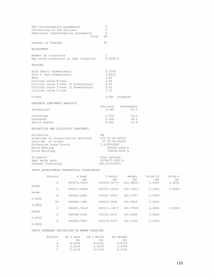
110

GPS transformation parameters 0 Deflections of the vertical 0 Additional transformation parameters 0 Total 26 Degrees of freedom 55 ADJUSTMENT Number of iterations 1 Max coord correction in last iteration 0.0000 m TESTING Alfa (multi dimensional) 0.2790 Alfa 0 (one dimensional) 0.0010 Beta 0.80 Critical value W-test 3.29 Critical value T-test (3 dimensional) 4.24 Critical value T-test (2 dimensional) 5.91 Critical value F-test 1.10 F-test 0.048 accepted VARIANCE COMPONENT ANALYSIS Variance Redundancy Terrestrial 0.025 53.1 Directions 0.076 15.0 Distances 0.008 18.2 Zenith angles 0.002 19.9 PROJECTION AND ELLIPSOID CONSTANTS Projection TM Longitude of origin/central meridian 272 55 00.00000 Latitude of origin 37 30 00.00000 Projection scale factor 1.000000000 False Easting 900000.0000 m False Northing 250000.0000 m Ellipsoid User defined Semi major axis 6378137.0000 m Inverse flattening 298.257223563 INPUT APPROXIMATE TERRESTRIAL COORDINATES Station X East Y North Height Id.Sd XY Id.Sd h (m) (m) (m) (m) (m) A 965475.3293* 493269.5677* 201.8801* 0.0000 0.0000 known F 965473.5608* 493257.3024* 201.7891* 0.0000 0.0000 known B 965465.2982 493287.0832 201.9307 0.0000 0.0000 TS 965485.1986 493253.3956 201.5810 0.0000 0.0000 C 965451.7614* 493311.1451* 201.7783* 0.0000 0.0000 known D 965448.6186 493301.0872 201.6469 0.0000 0.0000 E 965460.9926 493279.4072 201.9320 0.0000 0.0000 INPUT STANDARD DEVIATIONS OF KNOWN STATIONS Station Sd X East Sd Y North Sd Height (m) (m) (m) A 0.0100 0.0100 0.0100 F 0.0100 0.0100 0.0100 C 0.0100 0.0100 0.0100

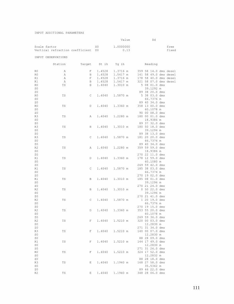
111

INPUT ADDITIONAL PARAMETERS Value Sd Scale factor S0 1.0000000 free Vertical refraction coefficient Z0 0.13 fixed INPUT OBSERVATIONS Station Target St ih Tg ih Reading R0 A F 1.4528 1.3716 m 359 58 14.0 dms desel R0 A B 1.4528 1.5417 m 141 58 49.0 dms desel R1 A F 1.4528 1.3716 m 178 58 40.0 dms desel R1 A B 1.4528 1.5417 m 321 58 07.0 dms desel R0 TS B 1.4040 1.3010 m 5 08 01.0 dms S0 39.1292 m Z0 89 38 20.0 dms R0 TS C 1.4040 1.5870 m 5 38 03.0 dms S0 66.7376 m Z0 89 40 34.0 dms R0 TS D 1.4040 1.3360 m 358 13 00.0 dms S0 60.1078 m Z0 90 00 08.0 dms R3 TS A 1.4040 1.2280 m 180 00 01.0 dms S0 18.9386 m Z0 89 37 32.0 dms R3 TS B 1.4040 1.3010 m 180 50 18.0 dms S0 39.1294 m Z0 89 38 13.0 dms R3 TS C 1.4040 1.5870 m 181 20 20.0 dms S0 66.7376 m Z0 89 40 34.0 dms R2 TS A 1.4040 1.2280 m 359 59 59.0 dms S0 18.9386 m Z0 270 22 11.0 dms R1 TS D 1.4040 1.3360 m 178 12 59.0 dms S0 60.1080 m Z0 269 59 42.0 dms R1 TS C 1.4040 1.5870 m 185 38 03.0 dms S0 66.7374 m Z0 270 19 02.0 dms R1 TS B 1.4040 1.3010 m 185 08 01.0 dms S0 39.1296 m Z0 270 21 24.0 dms R2 TS B 1.4040 1.3010 m 0 50 22.0 dms S0 39.1296 m Z0 270 21 41.0 dms R2 TS C 1.4040 1.5870 m 1 20 19.0 dms S0 66.7376 m Z0 270 19 15.0 dms R2 TS D 1.4040 1.3360 m 353 55 20.0 dms S0 60.1078 m Z0 269 59 36.0 dms R2 TS F 1.4040 1.5210 m 320 00 03.0 dms S0 12.2830 m Z0 271 31 34.0 dms R3 TS F 1.4040 1.5210 m 140 00 07.0 dms S0 12.2830 m Z0 88 28 09.0 dms R1 TS F 1.4040 1.5210 m 144 17 49.0 dms S0 12.2830 m Z0 271 31 26.0 dms R0 TS F 1.4040 1.5210 m 324 17 52.0 dms S0 12.2832 m Z0 88 28 18.0 dms R3 TS E 1.4040 1.1940 m 168 27 58.0 dms S0 35.5342 m Z0 89 46 22.0 dms R2 TS E 1.4040 1.1940 m 348 28 06.0 dms

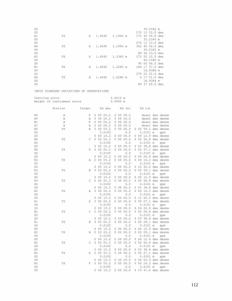
112

S0 35.5342 m Z0 270 13 25.0 dms R1 TS E 1.4040 1.1940 m 172 45 45.0 dms S0 35.5340 m Z0 270 13 33.0 dms R0 TS E 1.4040 1.1940 m 352 45 52.0 dms S0 35.5342 m Z0 89 46 23.0 dms R3 TS D 1.4040 1.3360 m 173 55 15.0 dms S0 60.1080 m Z0 90 00 06.0 dms R1 TS A 1.4040 1.2280 m 184 17 37.0 dms S0 18.9386 m Z0 270 22 22.0 dms R0 TS A 1.4040 1.2280 m 4 17 51.0 dms S0 18.9384 m Z0 89 37 24.0 dms INPUT STANDARD DEVIATIONS OF OBSERVATIONS Centring error 0.0010 m Height of instrument error 0.0500 m Station Target Sd abs Sd rel Sd tot R0 A F 0 00 05.2 0 00 00.0 desel dms dmskm R0 A B 0 00 05.2 0 00 00.0 desel dms dmskm R1 A F 0 00 05.2 0 00 00.0 desel dms dmskm R1 A B 0 00 05.2 0 00 00.0 desel dms dmskm R0 TS B 0 00 05.2 0 00 00.0 0 00 09.1 dms dmskm S0 0.0100 0.0 0.0101 m ppm Z0 0 00 10.2 0 00 00.0 0 06 12.9 dms dmskm R0 TS C 0 00 05.2 0 00 00.0 0 00 06.8 dms dmskm S0 0.0100 0.0 0.0101 m ppm Z0 0 00 10.2 0 00 00.0 0 03 38.8 dms dmskm R0 TS D 0 00 05.2 0 00 00.0 0 00 07.1 dms dmskm S0 0.0100 0.0 0.0101 m ppm Z0 0 00 10.2 0 00 00.0 0 04 02.9 dms dmskm R3 TS A 0 00 05.2 0 00 00.0 0 00 16.3 dms dmskm S0 0.0100 0.0 0.0101 m ppm Z0 0 00 10.2 0 00 00.0 0 12 50.2 dms dmskm R3 TS B 0 00 05.2 0 00 00.0 0 00 09.1 dms dmskm S0 0.0100 0.0 0.0101 m ppm Z0 0 00 10.2 0 00 00.0 0 06 12.9 dms dmskm R3 TS C 0 00 05.2 0 00 00.0 0 00 06.8 dms dmskm S0 0.0100 0.0 0.0101 m ppm Z0 0 00 10.2 0 00 00.0 0 03 38.8 dms dmskm R2 TS A 0 00 05.2 0 00 00.0 0 00 16.3 dms dmskm S0 0.0100 0.0 0.0101 m ppm Z0 0 00 10.2 0 00 00.0 0 12 50.2 dms dmskm R1 TS D 0 00 05.2 0 00 00.0 0 00 07.1 dms dmskm S0 0.0100 0.0 0.0101 m ppm Z0 0 00 10.2 0 00 00.0 0 04 02.9 dms dmskm R1 TS C 0 00 05.2 0 00 00.0 0 00 06.8 dms dmskm S0 0.0100 0.0 0.0101 m ppm Z0 0 00 10.2 0 00 00.0 0 03 38.8 dms dmskm R1 TS B 0 00 05.2 0 00 00.0 0 00 09.1 dms dmskm S0 0.0100 0.0 0.0101 m ppm Z0 0 00 10.2 0 00 00.0 0 06 12.9 dms dmskm R2 TS B 0 00 05.2 0 00 00.0 0 00 09.1 dms dmskm S0 0.0100 0.0 0.0101 m ppm Z0 0 00 10.2 0 00 00.0 0 06 12.9 dms dmskm R2 TS C 0 00 05.2 0 00 00.0 0 00 06.8 dms dmskm S0 0.0100 0.0 0.0101 m ppm Z0 0 00 10.2 0 00 00.0 0 03 38.8 dms dmskm R2 TS D 0 00 05.2 0 00 00.0 0 00 07.1 dms dmskm S0 0.0100 0.0 0.0101 m ppm Z0 0 00 10.2 0 00 00.0 0 04 02.9 dms dmskm R2 TS F 0 00 05.2 0 00 00.0 0 00 24.3 dms dmskm S0 0.0100 0.0 0.0101 m ppm Z0 0 00 10.2 0 00 00.0 0 19 47.6 dms dmskm

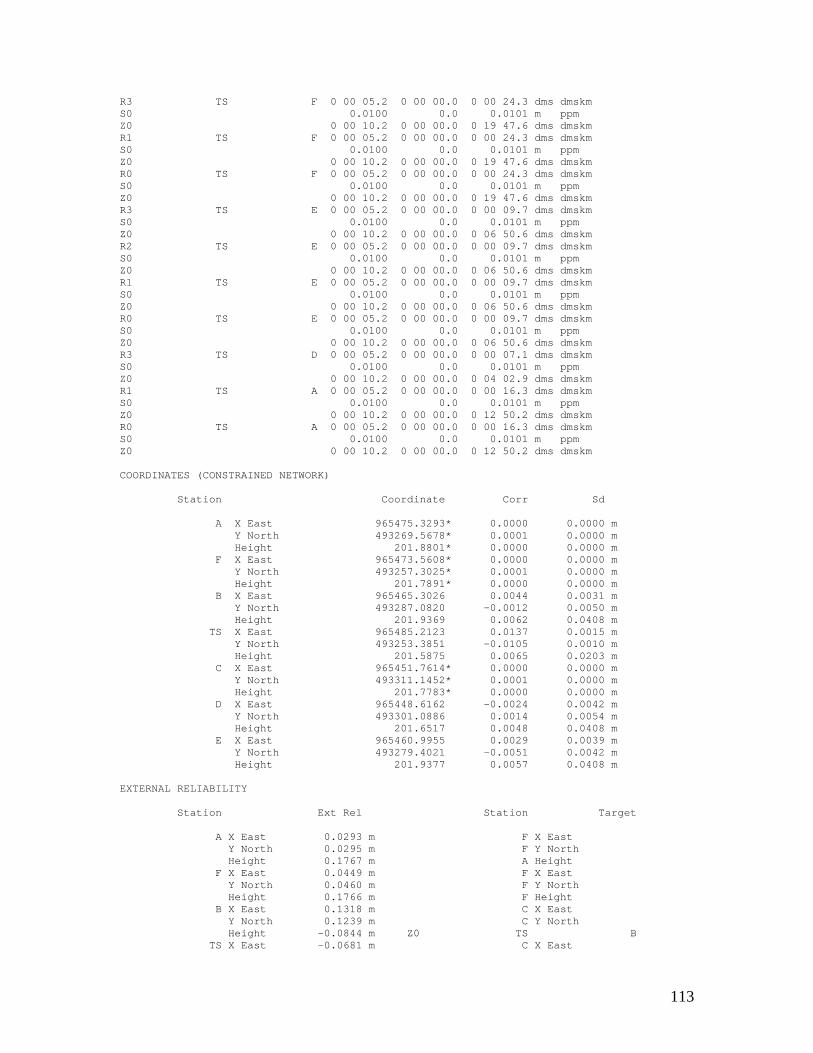
113

R3 TS F 0 00 05.2 0 00 00.0 0 00 24.3 dms dmskm S0 0.0100 0.0 0.0101 m ppm Z0 0 00 10.2 0 00 00.0 0 19 47.6 dms dmskm R1 TS F 0 00 05.2 0 00 00.0 0 00 24.3 dms dmskm S0 0.0100 0.0 0.0101 m ppm Z0 0 00 10.2 0 00 00.0 0 19 47.6 dms dmskm R0 TS F 0 00 05.2 0 00 00.0 0 00 24.3 dms dmskm S0 0.0100 0.0 0.0101 m ppm Z0 0 00 10.2 0 00 00.0 0 19 47.6 dms dmskm R3 TS E 0 00 05.2 0 00 00.0 0 00 09.7 dms dmskm S0 0.0100 0.0 0.0101 m ppm Z0 0 00 10.2 0 00 00.0 0 06 50.6 dms dmskm R2 TS E 0 00 05.2 0 00 00.0 0 00 09.7 dms dmskm S0 0.0100 0.0 0.0101 m ppm Z0 0 00 10.2 0 00 00.0 0 06 50.6 dms dmskm R1 TS E 0 00 05.2 0 00 00.0 0 00 09.7 dms dmskm S0 0.0100 0.0 0.0101 m ppm Z0 0 00 10.2 0 00 00.0 0 06 50.6 dms dmskm R0 TS E 0 00 05.2 0 00 00.0 0 00 09.7 dms dmskm S0 0.0100 0.0 0.0101 m ppm Z0 0 00 10.2 0 00 00.0 0 06 50.6 dms dmskm R3 TS D 0 00 05.2 0 00 00.0 0 00 07.1 dms dmskm S0 0.0100 0.0 0.0101 m ppm Z0 0 00 10.2 0 00 00.0 0 04 02.9 dms dmskm R1 TS A 0 00 05.2 0 00 00.0 0 00 16.3 dms dmskm S0 0.0100 0.0 0.0101 m ppm Z0 0 00 10.2 0 00 00.0 0 12 50.2 dms dmskm R0 TS A 0 00 05.2 0 00 00.0 0 00 16.3 dms dmskm S0 0.0100 0.0 0.0101 m ppm Z0 0 00 10.2 0 00 00.0 0 12 50.2 dms dmskm COORDINATES (CONSTRAINED NETWORK) Station Coordinate Corr Sd A X East 965475.3293* 0.0000 0.0000 m Y North 493269.5678* 0.0001 0.0000 m Height 201.8801* 0.0000 0.0000 m F X East 965473.5608* 0.0000 0.0000 m Y North 493257.3025* 0.0001 0.0000 m Height 201.7891* 0.0000 0.0000 m B X East 965465.3026 0.0044 0.0031 m Y North 493287.0820 -0.0012 0.0050 m Height 201.9369 0.0062 0.0408 m TS X East 965485.2123 0.0137 0.0015 m Y North 493253.3851 -0.0105 0.0010 m Height 201.5875 0.0065 0.0203 m C X East 965451.7614* 0.0000 0.0000 m Y North 493311.1452* 0.0001 0.0000 m Height 201.7783* 0.0000 0.0000 m D X East 965448.6162 -0.0024 0.0042 m Y North 493301.0886 0.0014 0.0054 m Height 201.6517 0.0048 0.0408 m E X East 965460.9955 0.0029 0.0039 m Y North 493279.4021 -0.0051 0.0042 m Height 201.9377 0.0057 0.0408 m EXTERNAL RELIABILITY Station Ext Rel Station Target A X East 0.0293 m F X East Y North 0.0295 m F Y North Height 0.1767 m A Height F X East 0.0449 m F X East Y North 0.0460 m F Y North Height 0.1766 m F Height B X East 0.1318 m C X East Y North 0.1239 m C Y North Height -0.0844 m Z0 TS B TS X East -0.0681 m C X East

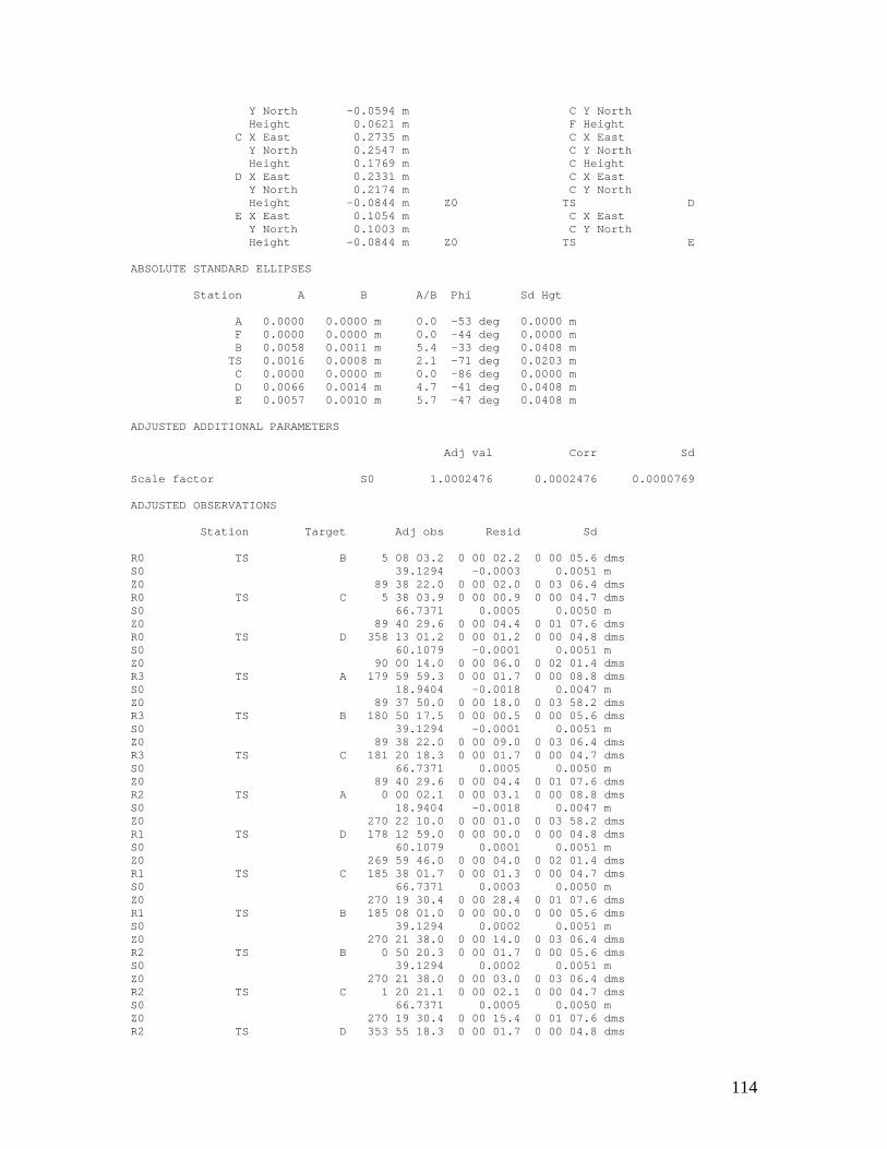
114

Y North -0.0594 m C Y North Height 0.0621 m F Height C X East 0.2735 m C X East Y North 0.2547 m C Y North Height 0.1769 m C Height D X East 0.2331 m C X East Y North 0.2174 m C Y North Height -0.0844 m Z0 TS D E X East 0.1054 m C X East Y North 0.1003 m C Y North Height -0.0844 m Z0 TS E ABSOLUTE STANDARD ELLIPSES Station A B A/B Phi Sd Hgt A 0.0000 0.0000 m 0.0 -53 deg 0.0000 m F 0.0000 0.0000 m 0.0 -44 deg 0.0000 m B 0.0058 0.0011 m 5.4 -33 deg 0.0408 m TS 0.0016 0.0008 m 2.1 -71 deg 0.0203 m C 0.0000 0.0000 m 0.0 -86 deg 0.0000 m D 0.0066 0.0014 m 4.7 -41 deg 0.0408 m E 0.0057 0.0010 m 5.7 -47 deg 0.0408 m ADJUSTED ADDITIONAL PARAMETERS Adj val Corr Sd Scale factor S0 1.0002476 0.0002476 0.0000769 ADJUSTED OBSERVATIONS Station Target Adj obs Resid Sd R0 TS B 5 08 03.2 0 00 02.2 0 00 05.6 dms S0 39.1294 -0.0003 0.0051 m Z0 89 38 22.0 0 00 02.0 0 03 06.4 dms R0 TS C 5 38 03.9 0 00 00.9 0 00 04.7 dms S0 66.7371 0.0005 0.0050 m Z0 89 40 29.6 0 00 04.4 0 01 07.6 dms R0 TS D 358 13 01.2 0 00 01.2 0 00 04.8 dms S0 60.1079 -0.0001 0.0051 m Z0 90 00 14.0 0 00 06.0 0 02 01.4 dms R3 TS A 179 59 59.3 0 00 01.7 0 00 08.8 dms S0 18.9404 -0.0018 0.0047 m Z0 89 37 50.0 0 00 18.0 0 03 58.2 dms R3 TS B 180 50 17.5 0 00 00.5 0 00 05.6 dms S0 39.1294 -0.0001 0.0051 m Z0 89 38 22.0 0 00 09.0 0 03 06.4 dms R3 TS C 181 20 18.3 0 00 01.7 0 00 04.7 dms S0 66.7371 0.0005 0.0050 m Z0 89 40 29.6 0 00 04.4 0 01 07.6 dms R2 TS A 0 00 02.1 0 00 03.1 0 00 08.8 dms S0 18.9404 -0.0018 0.0047 m Z0 270 22 10.0 0 00 01.0 0 03 58.2 dms R1 TS D 178 12 59.0 0 00 00.0 0 00 04.8 dms S0 60.1079 0.0001 0.0051 m Z0 269 59 46.0 0 00 04.0 0 02 01.4 dms R1 TS C 185 38 01.7 0 00 01.3 0 00 04.7 dms S0 66.7371 0.0003 0.0050 m Z0 270 19 30.4 0 00 28.4 0 01 07.6 dms R1 TS B 185 08 01.0 0 00 00.0 0 00 05.6 dms S0 39.1294 0.0002 0.0051 m Z0 270 21 38.0 0 00 14.0 0 03 06.4 dms R2 TS B 0 50 20.3 0 00 01.7 0 00 05.6 dms S0 39.1294 0.0002 0.0051 m Z0 270 21 38.0 0 00 03.0 0 03 06.4 dms R2 TS C 1 20 21.1 0 00 02.1 0 00 04.7 dms S0 66.7371 0.0005 0.0050 m Z0 270 19 30.4 0 00 15.4 0 01 07.6 dms R2 TS D 353 55 18.3 0 00 01.7 0 00 04.8 dms

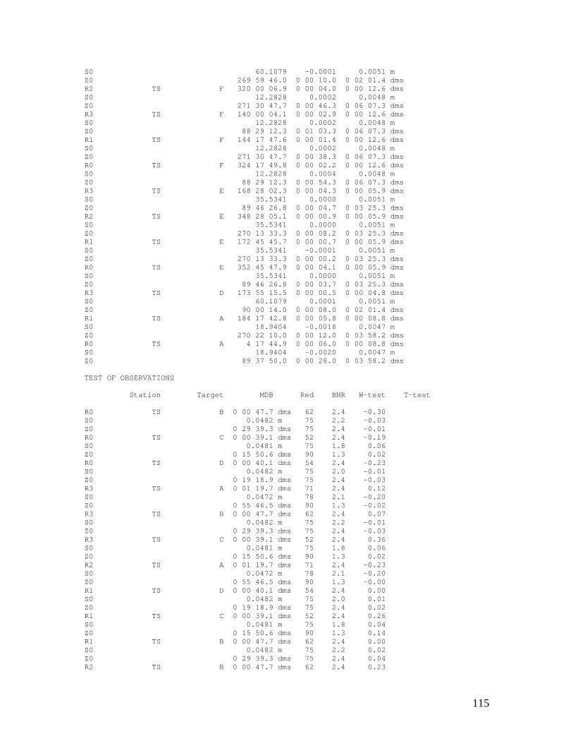
115

S0 60.1079 -0.0001 0.0051 m Z0 269 59 46.0 0 00 10.0 0 02 01.4 dms R2 TS F 320 00 06.9 0 00 04.0 0 00 12.6 dms S0 12.2828 0.0002 0.0048 m Z0 271 30 47.7 0 00 46.3 0 06 07.3 dms R3 TS F 140 00 04.1 0 00 02.9 0 00 12.6 dms S0 12.2828 0.0002 0.0048 m Z0 88 29 12.3 0 01 03.3 0 06 07.3 dms R1 TS F 144 17 47.6 0 00 01.4 0 00 12.6 dms S0 12.2828 0.0002 0.0048 m Z0 271 30 47.7 0 00 38.3 0 06 07.3 dms R0 TS F 324 17 49.8 0 00 02.2 0 00 12.6 dms S0 12.2828 0.0004 0.0048 m Z0 88 29 12.3 0 00 54.3 0 06 07.3 dms R3 TS E 168 28 02.3 0 00 04.3 0 00 05.9 dms S0 35.5341 0.0000 0.0051 m Z0 89 46 26.8 0 00 04.7 0 03 25.3 dms R2 TS E 348 28 05.1 0 00 00.9 0 00 05.9 dms S0 35.5341 0.0000 0.0051 m Z0 270 13 33.3 0 00 08.2 0 03 25.3 dms R1 TS E 172 45 45.7 0 00 00.7 0 00 05.9 dms S0 35.5341 -0.0001 0.0051 m Z0 270 13 33.3 0 00 00.2 0 03 25.3 dms R0 TS E 352 45 47.9 0 00 04.1 0 00 05.9 dms S0 35.5341 0.0000 0.0051 m Z0 89 46 26.8 0 00 03.7 0 03 25.3 dms R3 TS D 173 55 15.5 0 00 00.5 0 00 04.8 dms S0 60.1079 0.0001 0.0051 m Z0 90 00 14.0 0 00 08.0 0 02 01.4 dms R1 TS A 184 17 42.8 0 00 05.8 0 00 08.8 dms S0 18.9404 -0.0018 0.0047 m Z0 270 22 10.0 0 00 12.0 0 03 58.2 dms R0 TS A 4 17 44.9 0 00 06.0 0 00 08.8 dms S0 18.9404 -0.0020 0.0047 m Z0 89 37 50.0 0 00 26.0 0 03 58.2 dms TEST OF OBSERVATIONS Station Target MDB Red BNR W-test T-test R0 TS B 0 00 47.7 dms 62 2.4 -0.30 S0 0.0482 m 75 2.2 -0.03 Z0 0 29 39.3 dms 75 2.4 -0.01 R0 TS C 0 00 39.1 dms 52 2.4 -0.19 S0 0.0481 m 75 1.8 0.06 Z0 0 15 50.6 dms 90 1.3 0.02 R0 TS D 0 00 40.1 dms 54 2.4 -0.23 S0 0.0482 m 75 2.0 -0.01 Z0 0 19 18.9 dms 75 2.4 -0.03 R3 TS A 0 01 19.7 dms 71 2.4 0.12 S0 0.0472 m 78 2.1 -0.20 Z0 0 55 46.5 dms 90 1.3 -0.02 R3 TS B 0 00 47.7 dms 62 2.4 0.07 S0 0.0482 m 75 2.2 -0.01 Z0 0 29 39.3 dms 75 2.4 -0.03 R3 TS C 0 00 39.1 dms 52 2.4 0.36 S0 0.0481 m 75 1.8 0.06 Z0 0 15 50.6 dms 90 1.3 0.02 R2 TS A 0 01 19.7 dms 71 2.4 -0.23 S0 0.0472 m 78 2.1 -0.20 Z0 0 55 46.5 dms 90 1.3 -0.00 R1 TS D 0 00 40.1 dms 54 2.4 0.00 S0 0.0482 m 75 2.0 0.01 Z0 0 19 18.9 dms 75 2.4 0.02 R1 TS C 0 00 39.1 dms 52 2.4 0.26 S0 0.0481 m 75 1.8 0.04 Z0 0 15 50.6 dms 90 1.3 0.14 R1 TS B 0 00 47.7 dms 62 2.4 0.00 S0 0.0482 m 75 2.2 0.02 Z0 0 29 39.3 dms 75 2.4 0.04 R2 TS B 0 00 47.7 dms 62 2.4 0.23

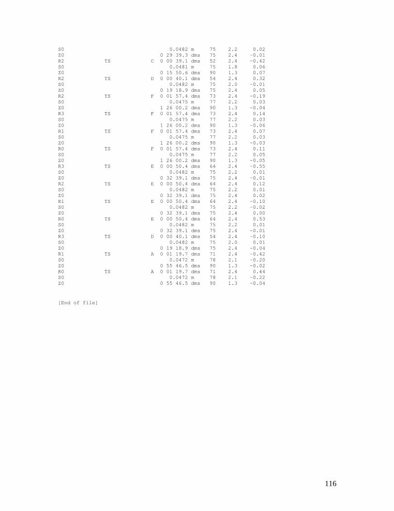
116

S0 0.0482 m 75 2.2 0.02 Z0 0 29 39.3 dms 75 2.4 -0.01 R2 TS C 0 00 39.1 dms 52 2.4 -0.42 S0 0.0481 m 75 1.8 0.06 Z0 0 15 50.6 dms 90 1.3 0.07 R2 TS D 0 00 40.1 dms 54 2.4 0.32 S0 0.0482 m 75 2.0 -0.01 Z0 0 19 18.9 dms 75 2.4 0.05 R2 TS F 0 01 57.4 dms 73 2.4 -0.19 S0 0.0475 m 77 2.2 0.03 Z0 1 26 00.2 dms 90 1.3 -0.04 R3 TS F 0 01 57.4 dms 73 2.4 0.14 S0 0.0475 m 77 2.2 0.03 Z0 1 26 00.2 dms 90 1.3 -0.06 R1 TS F 0 01 57.4 dms 73 2.4 0.07 S0 0.0475 m 77 2.2 0.03 Z0 1 26 00.2 dms 90 1.3 -0.03 R0 TS F 0 01 57.4 dms 73 2.4 0.11 S0 0.0475 m 77 2.2 0.05 Z0 1 26 00.2 dms 90 1.3 -0.05 R3 TS E 0 00 50.4 dms 64 2.4 -0.55 S0 0.0482 m 75 2.2 0.01 Z0 0 32 39.1 dms 75 2.4 -0.01 R2 TS E 0 00 50.4 dms 64 2.4 0.12 S0 0.0482 m 75 2.2 0.01 Z0 0 32 39.1 dms 75 2.4 0.02 R1 TS E 0 00 50.4 dms 64 2.4 -0.10 S0 0.0482 m 75 2.2 -0.02 Z0 0 32 39.1 dms 75 2.4 0.00 R0 TS E 0 00 50.4 dms 64 2.4 0.53 S0 0.0482 m 75 2.2 0.01 Z0 0 32 39.1 dms 75 2.4 -0.01 R3 TS D 0 00 40.1 dms 54 2.4 -0.10 S0 0.0482 m 75 2.0 0.01 Z0 0 19 18.9 dms 75 2.4 -0.04 R1 TS A 0 01 19.7 dms 71 2.4 -0.42 S0 0.0472 m 78 2.1 -0.20 Z0 0 55 46.5 dms 90 1.3 -0.02 R0 TS A 0 01 19.7 dms 71 2.4 0.44 S0 0.0472 m 78 2.1 -0.22 Z0 0 55 46.5 dms 90 1.3 -0.04

[End of file]

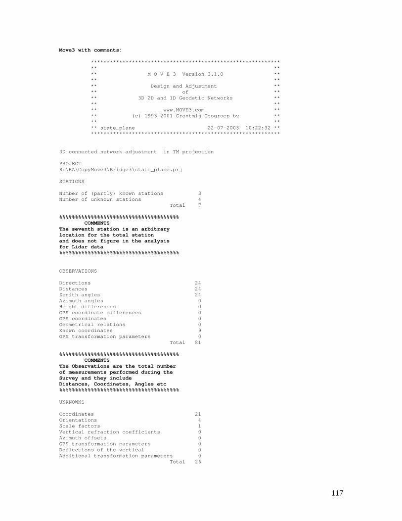
117

Move3 with comments: ************************************************************ ** ** ** M O V E 3 Version 3.1.0 ** ** ** ** Design and Adjustment ** ** of ** ** 3D 2D and 1D Geodetic Networks ** ** ** ** www.MOVE3.com ** ** (c) 1993-2001 Grontmij Geogroep bv ** ** ** ** state_plane 22-07-2003 10:22:32 ** ************************************************************ 3D connected network adjustment in TM projection PROJECT R:\RA\CopyMove3\Bridge3\state_plane.prj STATIONS Number of (partly) known stations 3 Number of unknown stations 4 Total 7 %%%%%%%%%%%%%%%%%%%%%%%%%%%%%%%%%%%%%% COMMENTS The seventh station is an arbitrary location for the total station and does not figure in the analysis for Lidar data %%%%%%%%%%%%%%%%%%%%%%%%%%%%%%%%%%%%%% OBSERVATIONS Directions 24 Distances 24 Zenith angles 24 Azimuth angles 0 Height differences 0 GPS coordinate differences 0 GPS coordinates 0 Geometrical relations 0 Known coordinates 9 GPS transformation parameters 0 Total 81 %%%%%%%%%%%%%%%%%%%%%%%%%%%%%%%%%%%%%% COMMENTS The Observations are the total number of measurements performed during the Survey and they include Distances, Coordinates, Angles etc %%%%%%%%%%%%%%%%%%%%%%%%%%%%%%%%%%%%%% UNKNOWNS Coordinates 21 Orientations 4 Scale factors 1 Vertical refraction coefficients 0 Azimuth offsets 0 GPS transformation parameters 0 Deflections of the vertical 0 Additional transformation parameters 0 Total 26

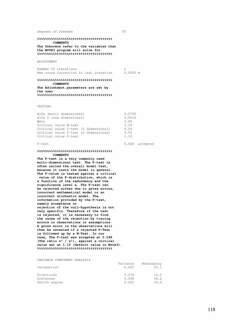
118

Degrees of freedom 55 %%%%%%%%%%%%%%%%%%%%%%%%%%%%%%%%%%%%%% COMMENTS The Unknowns refer to the variables that the MOVE3 program will solve for. %%%%%%%%%%%%%%%%%%%%%%%%%%%%%%%%%%%%%% ADJUSTMENT Number of iterations 1 Max coord correction in last iteration 0.0000 m %%%%%%%%%%%%%%%%%%%%%%%%%%%%%%%%%%%%%% COMMENTS The Adjustment parameters are set by the user. %%%%%%%%%%%%%%%%%%%%%%%%%%%%%%%%%%%%%% TESTING Alfa (multi dimensional) 0.2790 Alfa 0 (one dimensional) 0.0010 Beta 0.80 Critical value W-test 3.29 Critical value T-test (3 dimensional) 4.24 Critical value T-test (2 dimensional) 5.91 Critical value F-test 1.10 F-test 0.048 accepted %%%%%%%%%%%%%%%%%%%%%%%%%%%%%%%%%%%%%% COMMENTS The F-test is a very commonly used multi-dimensional test. The F-test is often called the overall model test, because it tests the model in general. The F-value is tested against a critical value of the F-distribution, which is a function of the redundancy and the significance level a. The F-test can be rejected either due to gross errors, incorrect mathematical model or an incorrect stochastic model. The information provided by the F-test, namely acceptance or rejection of the null-hypothesis is not very specific. Therefore if the test is rejected, it is necessary to find the cause of the rejection by tracing errors in observations or assumptions. A gross error is the observations will then be revealed if a rejected F-Test is followed up by a W-Test. In our case, The F-test was accepted at 0.048 (The ratio s² / s²), against a critical value set at 1.10 (default value in Move3). %%%%%%%%%%%%%%%%%%%%%%%%%%%%%%%%%%%%%% VARIANCE COMPONENT ANALYSIS Variance Redundancy Terrestrial 0.025 53.1 Directions 0.076 15.0 Distances 0.008 18.2 Zenith angles 0.002 19.9

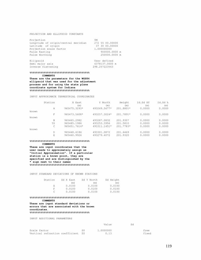
119

PROJECTION AND ELLIPSOID CONSTANTS Projection TM Longitude of origin/central meridian 272 55 00.00000 Latitude of origin 37 30 00.00000 Projection scale factor 1.000000000 False Easting 900000.0000 m False Northing 250000.0000 m Ellipsoid User defined Semi major axis 6378137.0000 m Inverse flattening 298.257223563 %%%%%%%%%%%%%%%%%%%%%%%%%%%%%%%%%%%%%% COMMENTS These are the parameters for the WGS84 ellipsoid that was used for the adjustment process and for using the state plane coordinate system for Indiana %%%%%%%%%%%%%%%%%%%%%%%%%%%%%%%%%%%%%% INPUT APPROXIMATE TERRESTRIAL COORDINATES Station X East Y North Height Id.Sd XY Id.Sd h (m) (m) (m) (m) (m) A 965475.3293* 493269.5677* 201.8801* 0.0000 0.0000 known F 965473.5608* 493257.3024* 201.7891* 0.0000 0.0000 known B 965465.2982 493287.0832 201.9307 0.0000 0.0000 TS 965485.1986 493253.3956 201.5810 0.0000 0.0000 C 965451.7614* 493311.1451* 201.7783* 0.0000 0.0000 known D 965448.6186 493301.0872 201.6469 0.0000 0.0000 E 965460.9926 493279.4072 201.9320 0.0000 0.0000 %%%%%%%%%%%%%%%%%%%%%%%%%%%%%%%%%%%%%% COMMENTS These are input coordinates that the user needs to apprximately assign as "Initial Approximation". If a particular station is a known point, they are specified and are distinguished by the * sign next to their names %%%%%%%%%%%%%%%%%%%%%%%%%%%%%%%%%%%%%% INPUT STANDARD DEVIATIONS OF KNOWN STATIONS Station Sd X East Sd Y North Sd Height (m) (m) (m) A 0.0100 0.0100 0.0100 F 0.0100 0.0100 0.0100 C 0.0100 0.0100 0.0100 %%%%%%%%%%%%%%%%%%%%%%%%%%%%%%%%%%%%%% COMMENTS These are input standard deviations or errors that are associated with the known coordinates. %%%%%%%%%%%%%%%%%%%%%%%%%%%%%%%%%%%%%% INPUT ADDITIONAL PARAMETERS Value Sd Scale factor S0 1.0000000 free Vertical refraction coefficient Z0 0.13 fixed

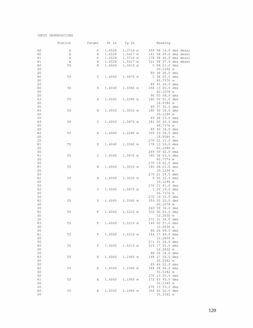
120

INPUT OBSERVATIONS Station Target St ih Tg ih Reading R0 A F 1.4528 1.3716 m 359 58 14.0 dms desel R0 A B 1.4528 1.5417 m 141 58 49.0 dms desel R1 A F 1.4528 1.3716 m 178 58 40.0 dms desel R1 A B 1.4528 1.5417 m 321 58 07.0 dms desel R0 TS B 1.4040 1.3010 m 5 08 01.0 dms S0 39.1292 m Z0 89 38 20.0 dms R0 TS C 1.4040 1.5870 m 5 38 03.0 dms S0 66.7376 m Z0 89 40 34.0 dms R0 TS D 1.4040 1.3360 m 358 13 00.0 dms S0 60.1078 m Z0 90 00 08.0 dms R3 TS A 1.4040 1.2280 m 180 00 01.0 dms S0 18.9386 m Z0 89 37 32.0 dms R3 TS B 1.4040 1.3010 m 180 50 18.0 dms S0 39.1294 m Z0 89 38 13.0 dms R3 TS C 1.4040 1.5870 m 181 20 20.0 dms S0 66.7376 m Z0 89 40 34.0 dms R2 TS A 1.4040 1.2280 m 359 59 59.0 dms S0 18.9386 m Z0 270 22 11.0 dms R1 TS D 1.4040 1.3360 m 178 12 59.0 dms S0 60.1080 m Z0 269 59 42.0 dms R1 TS C 1.4040 1.5870 m 185 38 03.0 dms S0 66.7374 m Z0 270 19 02.0 dms R1 TS B 1.4040 1.3010 m 185 08 01.0 dms S0 39.1296 m Z0 270 21 24.0 dms R2 TS B 1.4040 1.3010 m 0 50 22.0 dms S0 39.1296 m Z0 270 21 41.0 dms R2 TS C 1.4040 1.5870 m 1 20 19.0 dms S0 66.7376 m Z0 270 19 15.0 dms R2 TS D 1.4040 1.3360 m 353 55 20.0 dms S0 60.1078 m Z0 269 59 36.0 dms R2 TS F 1.4040 1.5210 m 320 00 03.0 dms S0 12.2830 m Z0 271 31 34.0 dms R3 TS F 1.4040 1.5210 m 140 00 07.0 dms S0 12.2830 m Z0 88 28 09.0 dms R1 TS F 1.4040 1.5210 m 144 17 49.0 dms S0 12.2830 m Z0 271 31 26.0 dms R0 TS F 1.4040 1.5210 m 324 17 52.0 dms S0 12.2832 m Z0 88 28 18.0 dms R3 TS E 1.4040 1.1940 m 168 27 58.0 dms S0 35.5342 m Z0 89 46 22.0 dms R2 TS E 1.4040 1.1940 m 348 28 06.0 dms S0 35.5342 m Z0 270 13 25.0 dms R1 TS E 1.4040 1.1940 m 172 45 45.0 dms S0 35.5340 m Z0 270 13 33.0 dms R0 TS E 1.4040 1.1940 m 352 45 52.0 dms S0 35.5342 m

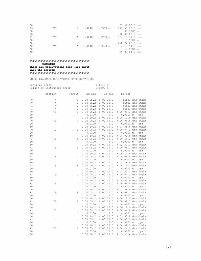
121

Z0 89 46 23.0 dms R3 TS D 1.4040 1.3360 m 173 55 15.0 dms S0 60.1080 m Z0 90 00 06.0 dms R1 TS A 1.4040 1.2280 m 184 17 37.0 dms S0 18.9386 m Z0 270 22 22.0 dms R0 TS A 1.4040 1.2280 m 4 17 51.0 dms S0 18.9384 m Z0 89 37 24.0 dms %%%%%%%%%%%%%%%%%%%%%%%%%%%%%%%%%%%%%% COMMENTS These are Observations that were input into the program %%%%%%%%%%%%%%%%%%%%%%%%%%%%%%%%%%%%%% INPUT STANDARD DEVIATIONS OF OBSERVATIONS Centring error 0.0010 m Height of instrument error 0.0500 m Station Target Sd abs Sd rel Sd tot R0 A F 0 00 05.2 0 00 00.0 desel dms dmskm R0 A B 0 00 05.2 0 00 00.0 desel dms dmskm R1 A F 0 00 05.2 0 00 00.0 desel dms dmskm R1 A B 0 00 05.2 0 00 00.0 desel dms dmskm R0 TS B 0 00 05.2 0 00 00.0 0 00 09.1 dms dmskm S0 0.0100 0.0 0.0101 m ppm Z0 0 00 10.2 0 00 00.0 0 06 12.9 dms dmskm R0 TS C 0 00 05.2 0 00 00.0 0 00 06.8 dms dmskm S0 0.0100 0.0 0.0101 m ppm Z0 0 00 10.2 0 00 00.0 0 03 38.8 dms dmskm R0 TS D 0 00 05.2 0 00 00.0 0 00 07.1 dms dmskm S0 0.0100 0.0 0.0101 m ppm Z0 0 00 10.2 0 00 00.0 0 04 02.9 dms dmskm R3 TS A 0 00 05.2 0 00 00.0 0 00 16.3 dms dmskm S0 0.0100 0.0 0.0101 m ppm Z0 0 00 10.2 0 00 00.0 0 12 50.2 dms dmskm R3 TS B 0 00 05.2 0 00 00.0 0 00 09.1 dms dmskm S0 0.0100 0.0 0.0101 m ppm Z0 0 00 10.2 0 00 00.0 0 06 12.9 dms dmskm R3 TS C 0 00 05.2 0 00 00.0 0 00 06.8 dms dmskm S0 0.0100 0.0 0.0101 m ppm Z0 0 00 10.2 0 00 00.0 0 03 38.8 dms dmskm R2 TS A 0 00 05.2 0 00 00.0 0 00 16.3 dms dmskm S0 0.0100 0.0 0.0101 m ppm Z0 0 00 10.2 0 00 00.0 0 12 50.2 dms dmskm R1 TS D 0 00 05.2 0 00 00.0 0 00 07.1 dms dmskm S0 0.0100 0.0 0.0101 m ppm Z0 0 00 10.2 0 00 00.0 0 04 02.9 dms dmskm R1 TS C 0 00 05.2 0 00 00.0 0 00 06.8 dms dmskm S0 0.0100 0.0 0.0101 m ppm Z0 0 00 10.2 0 00 00.0 0 03 38.8 dms dmskm R1 TS B 0 00 05.2 0 00 00.0 0 00 09.1 dms dmskm S0 0.0100 0.0 0.0101 m ppm Z0 0 00 10.2 0 00 00.0 0 06 12.9 dms dmskm R2 TS B 0 00 05.2 0 00 00.0 0 00 09.1 dms dmskm S0 0.0100 0.0 0.0101 m ppm Z0 0 00 10.2 0 00 00.0 0 06 12.9 dms dmskm R2 TS C 0 00 05.2 0 00 00.0 0 00 06.8 dms dmskm S0 0.0100 0.0 0.0101 m ppm Z0 0 00 10.2 0 00 00.0 0 03 38.8 dms dmskm R2 TS D 0 00 05.2 0 00 00.0 0 00 07.1 dms dmskm S0 0.0100 0.0 0.0101 m ppm Z0 0 00 10.2 0 00 00.0 0 04 02.9 dms dmskm R2 TS F 0 00 05.2 0 00 00.0 0 00 24.3 dms dmskm S0 0.0100 0.0 0.0101 m ppm Z0 0 00 10.2 0 00 00.0 0 19 47.6 dms dmskm

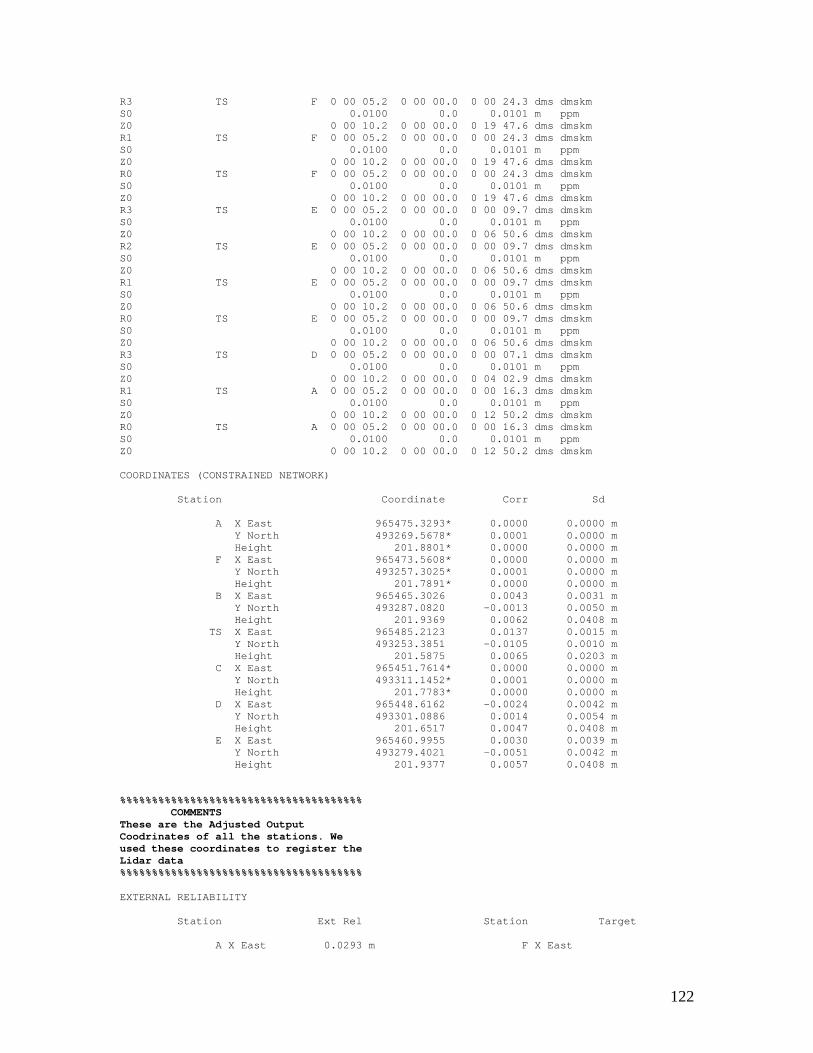
122

R3 TS F 0 00 05.2 0 00 00.0 0 00 24.3 dms dmskm S0 0.0100 0.0 0.0101 m ppm Z0 0 00 10.2 0 00 00.0 0 19 47.6 dms dmskm R1 TS F 0 00 05.2 0 00 00.0 0 00 24.3 dms dmskm S0 0.0100 0.0 0.0101 m ppm Z0 0 00 10.2 0 00 00.0 0 19 47.6 dms dmskm R0 TS F 0 00 05.2 0 00 00.0 0 00 24.3 dms dmskm S0 0.0100 0.0 0.0101 m ppm Z0 0 00 10.2 0 00 00.0 0 19 47.6 dms dmskm R3 TS E 0 00 05.2 0 00 00.0 0 00 09.7 dms dmskm S0 0.0100 0.0 0.0101 m ppm Z0 0 00 10.2 0 00 00.0 0 06 50.6 dms dmskm R2 TS E 0 00 05.2 0 00 00.0 0 00 09.7 dms dmskm S0 0.0100 0.0 0.0101 m ppm Z0 0 00 10.2 0 00 00.0 0 06 50.6 dms dmskm R1 TS E 0 00 05.2 0 00 00.0 0 00 09.7 dms dmskm S0 0.0100 0.0 0.0101 m ppm Z0 0 00 10.2 0 00 00.0 0 06 50.6 dms dmskm R0 TS E 0 00 05.2 0 00 00.0 0 00 09.7 dms dmskm S0 0.0100 0.0 0.0101 m ppm Z0 0 00 10.2 0 00 00.0 0 06 50.6 dms dmskm R3 TS D 0 00 05.2 0 00 00.0 0 00 07.1 dms dmskm S0 0.0100 0.0 0.0101 m ppm Z0 0 00 10.2 0 00 00.0 0 04 02.9 dms dmskm R1 TS A 0 00 05.2 0 00 00.0 0 00 16.3 dms dmskm S0 0.0100 0.0 0.0101 m ppm Z0 0 00 10.2 0 00 00.0 0 12 50.2 dms dmskm R0 TS A 0 00 05.2 0 00 00.0 0 00 16.3 dms dmskm S0 0.0100 0.0 0.0101 m ppm Z0 0 00 10.2 0 00 00.0 0 12 50.2 dms dmskm COORDINATES (CONSTRAINED NETWORK) Station Coordinate Corr Sd A X East 965475.3293* 0.0000 0.0000 m Y North 493269.5678* 0.0001 0.0000 m Height 201.8801* 0.0000 0.0000 m F X East 965473.5608* 0.0000 0.0000 m Y North 493257.3025* 0.0001 0.0000 m Height 201.7891* 0.0000 0.0000 m B X East 965465.3026 0.0043 0.0031 m Y North 493287.0820 -0.0013 0.0050 m Height 201.9369 0.0062 0.0408 m TS X East 965485.2123 0.0137 0.0015 m Y North 493253.3851 -0.0105 0.0010 m Height 201.5875 0.0065 0.0203 m C X East 965451.7614* 0.0000 0.0000 m Y North 493311.1452* 0.0001 0.0000 m Height 201.7783* 0.0000 0.0000 m D X East 965448.6162 -0.0024 0.0042 m Y North 493301.0886 0.0014 0.0054 m Height 201.6517 0.0047 0.0408 m E X East 965460.9955 0.0030 0.0039 m Y North 493279.4021 -0.0051 0.0042 m Height 201.9377 0.0057 0.0408 m %%%%%%%%%%%%%%%%%%%%%%%%%%%%%%%%%%%%%% COMMENTS These are the Adjusted Output Coodrinates of all the stations. We used these coordinates to register the Lidar data %%%%%%%%%%%%%%%%%%%%%%%%%%%%%%%%%%%%%% EXTERNAL RELIABILITY Station Ext Rel Station Target A X East 0.0293 m F X East

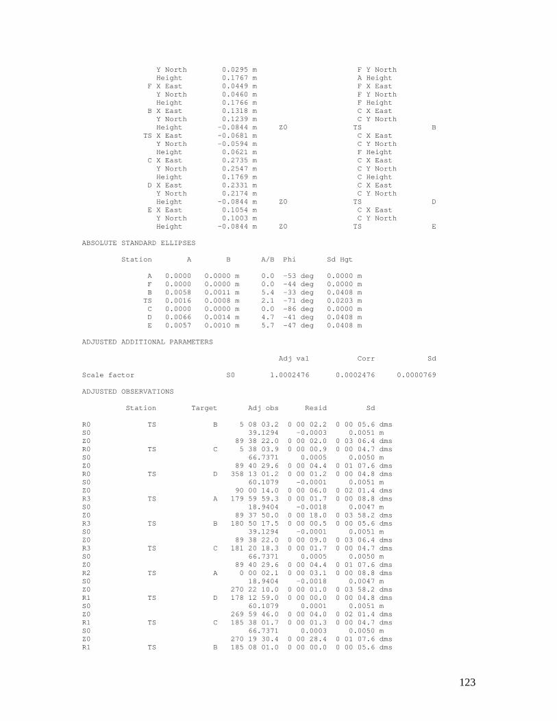
123

Y North 0.0295 m F Y North Height 0.1767 m A Height F X East 0.0449 m F X East Y North 0.0460 m F Y North Height 0.1766 m F Height B X East 0.1318 m C X East Y North 0.1239 m C Y North Height -0.0844 m Z0 TS B TS X East -0.0681 m C X East Y North -0.0594 m C Y North Height 0.0621 m F Height C X East 0.2735 m C X East Y North 0.2547 m C Y North Height 0.1769 m C Height D X East 0.2331 m C X East Y North 0.2174 m C Y North Height -0.0844 m Z0 TS D E X East 0.1054 m C X East Y North 0.1003 m C Y North Height -0.0844 m Z0 TS E ABSOLUTE STANDARD ELLIPSES Station A B A/B Phi Sd Hgt A 0.0000 0.0000 m 0.0 -53 deg 0.0000 m F 0.0000 0.0000 m 0.0 -44 deg 0.0000 m B 0.0058 0.0011 m 5.4 -33 deg 0.0408 m TS 0.0016 0.0008 m 2.1 -71 deg 0.0203 m C 0.0000 0.0000 m 0.0 -86 deg 0.0000 m D 0.0066 0.0014 m 4.7 -41 deg 0.0408 m E 0.0057 0.0010 m 5.7 -47 deg 0.0408 m ADJUSTED ADDITIONAL PARAMETERS Adj val Corr Sd Scale factor S0 1.0002476 0.0002476 0.0000769 ADJUSTED OBSERVATIONS Station Target Adj obs Resid Sd R0 TS B 5 08 03.2 0 00 02.2 0 00 05.6 dms S0 39.1294 -0.0003 0.0051 m Z0 89 38 22.0 0 00 02.0 0 03 06.4 dms R0 TS C 5 38 03.9 0 00 00.9 0 00 04.7 dms S0 66.7371 0.0005 0.0050 m Z0 89 40 29.6 0 00 04.4 0 01 07.6 dms R0 TS D 358 13 01.2 0 00 01.2 0 00 04.8 dms S0 60.1079 -0.0001 0.0051 m Z0 90 00 14.0 0 00 06.0 0 02 01.4 dms R3 TS A 179 59 59.3 0 00 01.7 0 00 08.8 dms S0 18.9404 -0.0018 0.0047 m Z0 89 37 50.0 0 00 18.0 0 03 58.2 dms R3 TS B 180 50 17.5 0 00 00.5 0 00 05.6 dms S0 39.1294 -0.0001 0.0051 m Z0 89 38 22.0 0 00 09.0 0 03 06.4 dms R3 TS C 181 20 18.3 0 00 01.7 0 00 04.7 dms S0 66.7371 0.0005 0.0050 m Z0 89 40 29.6 0 00 04.4 0 01 07.6 dms R2 TS A 0 00 02.1 0 00 03.1 0 00 08.8 dms S0 18.9404 -0.0018 0.0047 m Z0 270 22 10.0 0 00 01.0 0 03 58.2 dms R1 TS D 178 12 59.0 0 00 00.0 0 00 04.8 dms S0 60.1079 0.0001 0.0051 m Z0 269 59 46.0 0 00 04.0 0 02 01.4 dms R1 TS C 185 38 01.7 0 00 01.3 0 00 04.7 dms S0 66.7371 0.0003 0.0050 m Z0 270 19 30.4 0 00 28.4 0 01 07.6 dms R1 TS B 185 08 01.0 0 00 00.0 0 00 05.6 dms

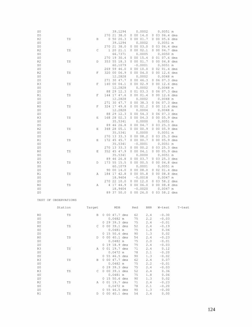
124

S0 39.1294 0.0002 0.0051 m Z0 270 21 38.0 0 00 14.0 0 03 06.4 dms R2 TS B 0 50 20.3 0 00 01.7 0 00 05.6 dms S0 39.1294 0.0002 0.0051 m Z0 270 21 38.0 0 00 03.0 0 03 06.4 dms R2 TS C 1 20 21.1 0 00 02.1 0 00 04.7 dms S0 66.7371 0.0005 0.0050 m Z0 270 19 30.4 0 00 15.4 0 01 07.6 dms R2 TS D 353 55 18.3 0 00 01.7 0 00 04.8 dms S0 60.1079 -0.0001 0.0051 m Z0 269 59 46.0 0 00 10.0 0 02 01.4 dms R2 TS F 320 00 06.9 0 00 04.0 0 00 12.6 dms S0 12.2828 0.0002 0.0048 m Z0 271 30 47.7 0 00 46.3 0 06 07.3 dms R3 TS F 140 00 04.1 0 00 02.9 0 00 12.6 dms S0 12.2828 0.0002 0.0048 m Z0 88 29 12.3 0 01 03.3 0 06 07.3 dms R1 TS F 144 17 47.6 0 00 01.4 0 00 12.6 dms S0 12.2828 0.0002 0.0048 m Z0 271 30 47.7 0 00 38.3 0 06 07.3 dms R0 TS F 324 17 49.8 0 00 02.2 0 00 12.6 dms S0 12.2828 0.0004 0.0048 m Z0 88 29 12.3 0 00 54.3 0 06 07.3 dms R3 TS E 168 28 02.3 0 00 04.3 0 00 05.9 dms S0 35.5341 0.0000 0.0051 m Z0 89 46 26.8 0 00 04.7 0 03 25.3 dms R2 TS E 348 28 05.1 0 00 00.9 0 00 05.9 dms S0 35.5341 0.0000 0.0051 m Z0 270 13 33.3 0 00 08.2 0 03 25.3 dms R1 TS E 172 45 45.7 0 00 00.7 0 00 05.9 dms S0 35.5341 -0.0001 0.0051 m Z0 270 13 33.3 0 00 00.2 0 03 25.3 dms R0 TS E 352 45 47.9 0 00 04.1 0 00 05.9 dms S0 35.5341 0.0000 0.0051 m Z0 89 46 26.8 0 00 03.7 0 03 25.3 dms R3 TS D 173 55 15.5 0 00 00.5 0 00 04.8 dms S0 60.1079 0.0001 0.0051 m Z0 90 00 14.0 0 00 08.0 0 02 01.4 dms R1 TS A 184 17 42.8 0 00 05.8 0 00 08.8 dms S0 18.9404 -0.0018 0.0047 m Z0 270 22 10.0 0 00 12.0 0 03 58.2 dms R0 TS A 4 17 44.9 0 00 06.0 0 00 08.8 dms S0 18.9404 -0.0020 0.0047 m Z0 89 37 50.0 0 00 26.0 0 03 58.2 dms TEST OF OBSERVATIONS Station Target MDB Red BNR W-test T-test R0 TS B 0 00 47.7 dms 62 2.4 -0.30 S0 0.0482 m 75 2.2 -0.03 Z0 0 29 39.3 dms 75 2.4 -0.01 R0 TS C 0 00 39.1 dms 52 2.4 -0.19 S0 0.0481 m 75 1.8 0.06 Z0 0 15 50.6 dms 90 1.3 0.02 R0 TS D 0 00 40.1 dms 54 2.4 -0.23 S0 0.0482 m 75 2.0 -0.01 Z0 0 19 18.9 dms 75 2.4 -0.03 R3 TS A 0 01 19.7 dms 71 2.4 0.12 S0 0.0472 m 78 2.1 -0.20 Z0 0 55 46.5 dms 90 1.3 -0.02 R3 TS B 0 00 47.7 dms 62 2.4 0.07 S0 0.0482 m 75 2.2 -0.01 Z0 0 29 39.3 dms 75 2.4 -0.03 R3 TS C 0 00 39.1 dms 52 2.4 0.36 S0 0.0481 m 75 1.8 0.06 Z0 0 15 50.6 dms 90 1.3 0.02 R2 TS A 0 01 19.7 dms 71 2.4 -0.23 S0 0.0472 m 78 2.1 -0.20 Z0 0 55 46.5 dms 90 1.3 -0.00 R1 TS D 0 00 40.1 dms 54 2.4 0.00

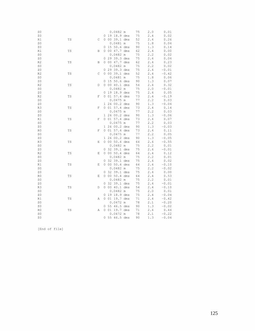
125

S0 0.0482 m 75 2.0 0.01 Z0 0 19 18.9 dms 75 2.4 0.02 R1 TS C 0 00 39.1 dms 52 2.4 0.26 S0 0.0481 m 75 1.8 0.04 Z0 0 15 50.6 dms 90 1.3 0.14 R1 TS B 0 00 47.7 dms 62 2.4 0.00 S0 0.0482 m 75 2.2 0.02 Z0 0 29 39.3 dms 75 2.4 0.04 R2 TS B 0 00 47.7 dms 62 2.4 0.23 S0 0.0482 m 75 2.2 0.02 Z0 0 29 39.3 dms 75 2.4 -0.01 R2 TS C 0 00 39.1 dms 52 2.4 -0.42 S0 0.0481 m 75 1.8 0.06 Z0 0 15 50.6 dms 90 1.3 0.07 R2 TS D 0 00 40.1 dms 54 2.4 0.32 S0 0.0482 m 75 2.0 -0.01 Z0 0 19 18.9 dms 75 2.4 0.05 R2 TS F 0 01 57.4 dms 73 2.4 -0.19 S0 0.0475 m 77 2.2 0.03 Z0 1 26 00.2 dms 90 1.3 -0.04 R3 TS F 0 01 57.4 dms 73 2.4 0.14 S0 0.0475 m 77 2.2 0.03 Z0 1 26 00.2 dms 90 1.3 -0.06 R1 TS F 0 01 57.4 dms 73 2.4 0.07 S0 0.0475 m 77 2.2 0.03 Z0 1 26 00.2 dms 90 1.3 -0.03 R0 TS F 0 01 57.4 dms 73 2.4 0.11 S0 0.0475 m 77 2.2 0.05 Z0 1 26 00.2 dms 90 1.3 -0.05 R3 TS E 0 00 50.4 dms 64 2.4 -0.55 S0 0.0482 m 75 2.2 0.01 Z0 0 32 39.1 dms 75 2.4 -0.01 R2 TS E 0 00 50.4 dms 64 2.4 0.12 S0 0.0482 m 75 2.2 0.01 Z0 0 32 39.1 dms 75 2.4 0.02 R1 TS E 0 00 50.4 dms 64 2.4 -0.10 S0 0.0482 m 75 2.2 -0.02 Z0 0 32 39.1 dms 75 2.4 0.00 R0 TS E 0 00 50.4 dms 64 2.4 0.53 S0 0.0482 m 75 2.2 0.01 Z0 0 32 39.1 dms 75 2.4 -0.01 R3 TS D 0 00 40.1 dms 54 2.4 -0.10 S0 0.0482 m 75 2.0 0.01 Z0 0 19 18.9 dms 75 2.4 -0.04 R1 TS A 0 01 19.7 dms 71 2.4 -0.42 S0 0.0472 m 78 2.1 -0.20 Z0 0 55 46.5 dms 90 1.3 -0.02 R0 TS A 0 01 19.7 dms 71 2.4 0.44 S0 0.0472 m 78 2.1 -0.22 Z0 0 55 46.5 dms 90 1.3 -0.04 [End of file]

126

APPENDIX E

Diagnostics of Registration within Cyclone

Mean Absolute Error: for Enabled Constraints = 0.004 m for Disabled Constraints = 0.000 m Date: 2003.06.17 13:39:26 Database name : Bridgeport ScanWorlds ScanWorld 1 ScanWorld 2 ScanWorld 3 ScanWorld 4 ScanWorld 5 ScanWorld 6 ScanWorld 7 FINAL_c6pts Constraints Name ScanWorld ScanWorld Type On/Off Weight Error Error Vector TargetID: S8 ScanWorld 1 ScanWorld 2 Coincident: Sphere-Sphere On 1.00 0.006 m (0.004, -0.003, 0.004) m TargetID: S4 ScanWorld 1 ScanWorld 2 Coincident: Sphere-Sphere On 1.00 0.006 m (0.001, -0.002, -0.005) m TargetID: S5 ScanWorld 1 ScanWorld 2 Coincident: Sphere-Sphere On 1.00 0.004 m (-0.001, 0.004, 0.000) m TargetID: S8 ScanWorld 1 ScanWorld 3 Coincident: Sphere-Sphere On 1.00 0.005 m (0.002, -0.001, 0.005) m TargetID: S4 ScanWorld 1 ScanWorld 3 Coincident: Sphere-Sphere On 1.00 0.001 m (0.000, 0.000, -0.001) m TargetID: S5 ScanWorld 1 ScanWorld 3 Coincident: Sphere-Sphere On 1.00 0.005 m (0.002, 0.001, -0.004) m TargetID: S8 ScanWorld 1 ScanWorld 4 Coincident: Sphere-Sphere On 1.00 0.007 m (0.003, -0.005, 0.003) m TargetID: S6 ScanWorld 1 ScanWorld 4 Coincident: Sphere-Sphere On 1.00 0.002 m (0.000, 0.001, -0.001) m TargetID: S4 ScanWorld 1 ScanWorld 4 Coincident: Sphere-Sphere On 1.00 0.005 m (0.000, 0.001, -0.005) m TargetID: S5 ScanWorld 1 ScanWorld 4 Coincident: Sphere-Sphere On 1.00 0.003 m (0.001, 0.003, -0.001) m TargetID: S3 ScanWorld 1 ScanWorld 4 Coincident: Sphere-Sphere On 1.00 0.004 m (-0.003, -0.002, 0.001) m TargetID: S2 ScanWorld 1 ScanWorld 4 Coincident: Sphere-Sphere On 1.00 0.004 m (-0.002, -0.001, 0.004) m TargetID: S1 ScanWorld 1 ScanWorld 4 Coincident: Sphere-Sphere On 1.00 0.002 m (0.000, 0.000, 0.002) m TargetID: S6 ScanWorld 1 ScanWorld 5 Coincident: Sphere-Sphere On 1.00 0.001 m (0.001, 0.000, -0.001) m TargetID: S4 ScanWorld 1 ScanWorld 5 Coincident: Sphere-Sphere On 1.00 0.005 m (0.001, -0.001, -0.005) m TargetID: S5 ScanWorld 1 ScanWorld 5 Coincident: Sphere-Sphere On 1.00 0.002 m (0.000, 0.002, -0.001) m TargetID: S3 ScanWorld 1 ScanWorld 5 Coincident: Sphere-Sphere On 1.00 0.003 m (-0.002, 0.000, 0.002) m TargetID: S2 ScanWorld 1 ScanWorld 5 Coincident: Sphere-Sphere On 1.00 0.003 m (-0.002, -0.001, 0.003) m TargetID: S1 ScanWorld 1 ScanWorld 5 Coincident: Sphere-Sphere On 1.00 0.002 m (0.000, 0.001, 0.002) m TargetID: S6 ScanWorld 1 ScanWorld 6 Coincident: Sphere-Sphere On 1.00 0.002 m (0.001, 0.002, -0.001) m TargetID: S4 ScanWorld 1 ScanWorld 6 Coincident: Sphere-Sphere On 1.00 0.005 m (0.001, -0.002, -0.004) m TargetID: S5 ScanWorld 1 ScanWorld 6 Coincident: Sphere-Sphere On 1.00 0.003 m (0.000, 0.002, -0.003) m TargetID: S3 ScanWorld 1 ScanWorld 6 Coincident: Sphere-Sphere On 1.00 0.004 m (-0.001, 0.001, 0.004) m TargetID: S7 ScanWorld 1 ScanWorld 6 Coincident: Sphere-Sphere On 1.00 0.003 m (-0.001, 0.002, -0.002) m TargetID: S2 ScanWorld 1 ScanWorld 6 Coincident: Sphere-Sphere On 1.00 0.004 m (-0.003, -0.001, 0.003) m TargetID: S1 ScanWorld 1 ScanWorld 6 Coincident: Sphere-Sphere On 1.00 0.003 m (0.002, -0.001, 0.002) m TargetID: S7 ScanWorld 1 ScanWorld 7 Coincident: Sphere-Sphere On 1.00 0.003 m (0.001, 0.001, -0.002) m TargetID: S2 ScanWorld 1 ScanWorld 7 Coincident: Sphere-Sphere On 1.00 0.006 m (-0.004, 0.000, 0.005) m TargetID: S1 ScanWorld 1 ScanWorld 7 Coincident: Sphere-Sphere On 1.00 0.002 m (0.000, -0.002, 0.000) m TargetID: S6 ScanWorld 1 FINAL_c6pts Coincident: Sphere-Vertex On 1.00 0.010 m (0.008, 0.004, -0.005) m TargetID: S4 ScanWorld 1 FINAL_c6pts Coincident: Sphere-Vertex On 1.00 0.004 m (0.001, -0.003, 0.002) m

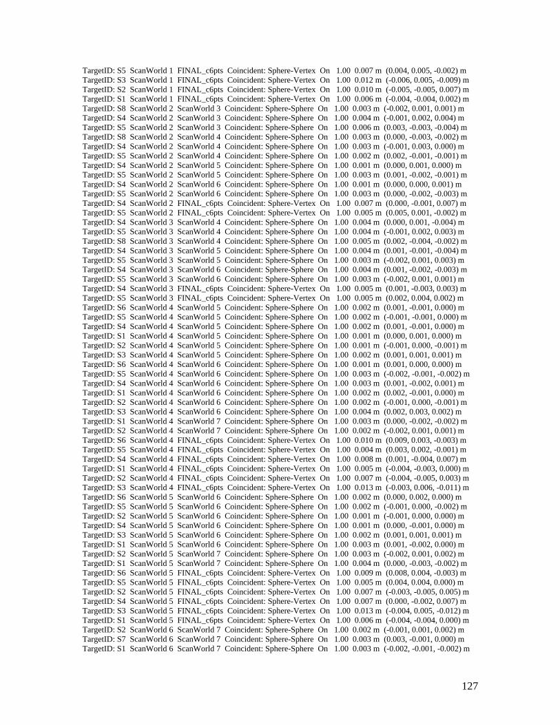
127

TargetID: S5 ScanWorld 1 FINAL_c6pts Coincident: Sphere-Vertex On 1.00 0.007 m (0.004, 0.005, -0.002) m TargetID: S3 ScanWorld 1 FINAL_c6pts Coincident: Sphere-Vertex On 1.00 0.012 m (-0.006, 0.005, -0.009) m TargetID: S2 ScanWorld 1 FINAL_c6pts Coincident: Sphere-Vertex On 1.00 0.010 m (-0.005, -0.005, 0.007) m TargetID: S1 ScanWorld 1 FINAL_c6pts Coincident: Sphere-Vertex On 1.00 0.006 m (-0.004, -0.004, 0.002) m TargetID: S8 ScanWorld 2 ScanWorld 3 Coincident: Sphere-Sphere On 1.00 0.003 m (-0.002, 0.001, 0.001) m TargetID: S4 ScanWorld 2 ScanWorld 3 Coincident: Sphere-Sphere On 1.00 0.004 m (-0.001, 0.002, 0.004) m TargetID: S5 ScanWorld 2 ScanWorld 3 Coincident: Sphere-Sphere On 1.00 0.006 m (0.003, -0.003, -0.004) m TargetID: S8 ScanWorld 2 ScanWorld 4 Coincident: Sphere-Sphere On 1.00 0.003 m (0.000, -0.003, -0.002) m TargetID: S4 ScanWorld 2 ScanWorld 4 Coincident: Sphere-Sphere On 1.00 0.003 m (-0.001, 0.003, 0.000) m TargetID: S5 ScanWorld 2 ScanWorld 4 Coincident: Sphere-Sphere On 1.00 0.002 m (0.002, -0.001, -0.001) m TargetID: S4 ScanWorld 2 ScanWorld 5 Coincident: Sphere-Sphere On 1.00 0.001 m (0.000, 0.001, 0.000) m TargetID: S5 ScanWorld 2 ScanWorld 5 Coincident: Sphere-Sphere On 1.00 0.003 m (0.001, -0.002, -0.001) m TargetID: S4 ScanWorld 2 ScanWorld 6 Coincident: Sphere-Sphere On 1.00 0.001 m (0.000, 0.000, 0.001) m TargetID: S5 ScanWorld 2 ScanWorld 6 Coincident: Sphere-Sphere On 1.00 0.003 m (0.000, -0.002, -0.003) m TargetID: S4 ScanWorld 2 FINAL_c6pts Coincident: Sphere-Vertex On 1.00 0.007 m (0.000, -0.001, 0.007) m TargetID: S5 ScanWorld 2 FINAL_c6pts Coincident: Sphere-Vertex On 1.00 0.005 m (0.005, 0.001, -0.002) m TargetID: S4 ScanWorld 3 ScanWorld 4 Coincident: Sphere-Sphere On 1.00 0.004 m (0.000, 0.001, -0.004) m TargetID: S5 ScanWorld 3 ScanWorld 4 Coincident: Sphere-Sphere On 1.00 0.004 m (-0.001, 0.002, 0.003) m TargetID: S8 ScanWorld 3 ScanWorld 4 Coincident: Sphere-Sphere On 1.00 0.005 m (0.002, -0.004, -0.002) m TargetID: S4 ScanWorld 3 ScanWorld 5 Coincident: Sphere-Sphere On 1.00 0.004 m (0.001, -0.001, -0.004) m TargetID: S5 ScanWorld 3 ScanWorld 5 Coincident: Sphere-Sphere On 1.00 0.003 m (-0.002, 0.001, 0.003) m TargetID: S4 ScanWorld 3 ScanWorld 6 Coincident: Sphere-Sphere On 1.00 0.004 m (0.001, -0.002, -0.003) m TargetID: S5 ScanWorld 3 ScanWorld 6 Coincident: Sphere-Sphere On 1.00 0.003 m (-0.002, 0.001, 0.001) m TargetID: S4 ScanWorld 3 FINAL_c6pts Coincident: Sphere-Vertex On 1.00 0.005 m (0.001, -0.003, 0.003) m TargetID: S5 ScanWorld 3 FINAL_c6pts Coincident: Sphere-Vertex On 1.00 0.005 m (0.002, 0.004, 0.002) m TargetID: S6 ScanWorld 4 ScanWorld 5 Coincident: Sphere-Sphere On 1.00 0.002 m (0.001, -0.001, 0.000) m TargetID: S5 ScanWorld 4 ScanWorld 5 Coincident: Sphere-Sphere On 1.00 0.002 m (-0.001, -0.001, 0.000) m TargetID: S4 ScanWorld 4 ScanWorld 5 Coincident: Sphere-Sphere On 1.00 0.002 m (0.001, -0.001, 0.000) m TargetID: S1 ScanWorld 4 ScanWorld 5 Coincident: Sphere-Sphere On 1.00 0.001 m (0.000, 0.001, 0.000) m TargetID: S2 ScanWorld 4 ScanWorld 5 Coincident: Sphere-Sphere On 1.00 0.001 m (-0.001, 0.000, -0.001) m TargetID: S3 ScanWorld 4 ScanWorld 5 Coincident: Sphere-Sphere On 1.00 0.002 m (0.001, 0.001, 0.001) m TargetID: S6 ScanWorld 4 ScanWorld 6 Coincident: Sphere-Sphere On 1.00 0.001 m (0.001, 0.000, 0.000) m TargetID: S5 ScanWorld 4 ScanWorld 6 Coincident: Sphere-Sphere On 1.00 0.003 m (-0.002, -0.001, -0.002) m TargetID: S4 ScanWorld 4 ScanWorld 6 Coincident: Sphere-Sphere On 1.00 0.003 m (0.001, -0.002, 0.001) m TargetID: S1 ScanWorld 4 ScanWorld 6 Coincident: Sphere-Sphere On 1.00 0.002 m (0.002, -0.001, 0.000) m TargetID: S2 ScanWorld 4 ScanWorld 6 Coincident: Sphere-Sphere On 1.00 0.002 m (-0.001, 0.000, -0.001) m TargetID: S3 ScanWorld 4 ScanWorld 6 Coincident: Sphere-Sphere On 1.00 0.004 m (0.002, 0.003, 0.002) m TargetID: S1 ScanWorld 4 ScanWorld 7 Coincident: Sphere-Sphere On 1.00 0.003 m (0.000, -0.002, -0.002) m TargetID: S2 ScanWorld 4 ScanWorld 7 Coincident: Sphere-Sphere On 1.00 0.002 m (-0.002, 0.001, 0.001) m TargetID: S6 ScanWorld 4 FINAL_c6pts Coincident: Sphere-Vertex On 1.00 0.010 m (0.009, 0.003, -0.003) m TargetID: S5 ScanWorld 4 FINAL_c6pts Coincident: Sphere-Vertex On 1.00 0.004 m (0.003, 0.002, -0.001) m TargetID: S4 ScanWorld 4 FINAL_c6pts Coincident: Sphere-Vertex On 1.00 0.008 m (0.001, -0.004, 0.007) m TargetID: S1 ScanWorld 4 FINAL_c6pts Coincident: Sphere-Vertex On 1.00 0.005 m (-0.004, -0.003, 0.000) m TargetID: S2 ScanWorld 4 FINAL_c6pts Coincident: Sphere-Vertex On 1.00 0.007 m (-0.004, -0.005, 0.003) m TargetID: S3 ScanWorld 4 FINAL_c6pts Coincident: Sphere-Vertex On 1.00 0.013 m (-0.003, 0.006, -0.011) m TargetID: S6 ScanWorld 5 ScanWorld 6 Coincident: Sphere-Sphere On 1.00 0.002 m (0.000, 0.002, 0.000) m TargetID: S5 ScanWorld 5 ScanWorld 6 Coincident: Sphere-Sphere On 1.00 0.002 m (-0.001, 0.000, -0.002) m TargetID: S2 ScanWorld 5 ScanWorld 6 Coincident: Sphere-Sphere On 1.00 0.001 m (-0.001, 0.000, 0.000) m TargetID: S4 ScanWorld 5 ScanWorld 6 Coincident: Sphere-Sphere On 1.00 0.001 m (0.000, -0.001, 0.000) m TargetID: S3 ScanWorld 5 ScanWorld 6 Coincident: Sphere-Sphere On 1.00 0.002 m (0.001, 0.001, 0.001) m TargetID: S1 ScanWorld 5 ScanWorld 6 Coincident: Sphere-Sphere On 1.00 0.003 m (0.001, -0.002, 0.000) m TargetID: S2 ScanWorld 5 ScanWorld 7 Coincident: Sphere-Sphere On 1.00 0.003 m (-0.002, 0.001, 0.002) m TargetID: S1 ScanWorld 5 ScanWorld 7 Coincident: Sphere-Sphere On 1.00 0.004 m (0.000, -0.003, -0.002) m TargetID: S6 ScanWorld 5 FINAL_c6pts Coincident: Sphere-Vertex On 1.00 0.009 m (0.008, 0.004, -0.003) m TargetID: S5 ScanWorld 5 FINAL_c6pts Coincident: Sphere-Vertex On 1.00 0.005 m (0.004, 0.004, 0.000) m TargetID: S2 ScanWorld 5 FINAL_c6pts Coincident: Sphere-Vertex On 1.00 0.007 m (-0.003, -0.005, 0.005) m TargetID: S4 ScanWorld 5 FINAL_c6pts Coincident: Sphere-Vertex On 1.00 0.007 m (0.000, -0.002, 0.007) m TargetID: S3 ScanWorld 5 FINAL_c6pts Coincident: Sphere-Vertex On 1.00 0.013 m (-0.004, 0.005, -0.012) m TargetID: S1 ScanWorld 5 FINAL_c6pts Coincident: Sphere-Vertex On 1.00 0.006 m (-0.004, -0.004, 0.000) m TargetID: S2 ScanWorld 6 ScanWorld 7 Coincident: Sphere-Sphere On 1.00 0.002 m (-0.001, 0.001, 0.002) m TargetID: S7 ScanWorld 6 ScanWorld 7 Coincident: Sphere-Sphere On 1.00 0.003 m (0.003, -0.001, 0.000) m TargetID: S1 ScanWorld 6 ScanWorld 7 Coincident: Sphere-Sphere On 1.00 0.003 m (-0.002, -0.001, -0.002) m

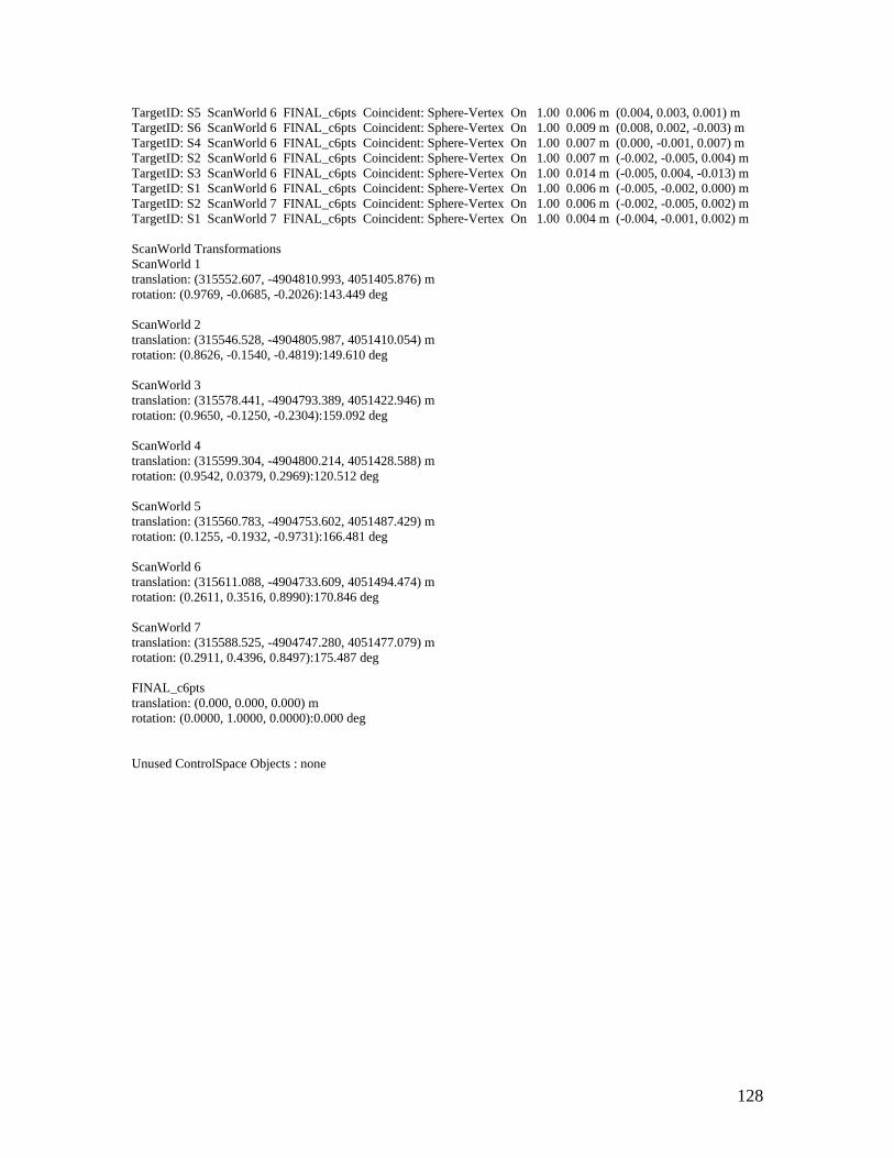
128

TargetID: S5 ScanWorld 6 FINAL_c6pts Coincident: Sphere-Vertex On 1.00 0.006 m (0.004, 0.003, 0.001) m TargetID: S6 ScanWorld 6 FINAL_c6pts Coincident: Sphere-Vertex On 1.00 0.009 m (0.008, 0.002, -0.003) m TargetID: S4 ScanWorld 6 FINAL_c6pts Coincident: Sphere-Vertex On 1.00 0.007 m (0.000, -0.001, 0.007) m TargetID: S2 ScanWorld 6 FINAL_c6pts Coincident: Sphere-Vertex On 1.00 0.007 m (-0.002, -0.005, 0.004) m TargetID: S3 ScanWorld 6 FINAL_c6pts Coincident: Sphere-Vertex On 1.00 0.014 m (-0.005, 0.004, -0.013) m TargetID: S1 ScanWorld 6 FINAL_c6pts Coincident: Sphere-Vertex On 1.00 0.006 m (-0.005, -0.002, 0.000) m TargetID: S2 ScanWorld 7 FINAL_c6pts Coincident: Sphere-Vertex On 1.00 0.006 m (-0.002, -0.005, 0.002) m TargetID: S1 ScanWorld 7 FINAL_c6pts Coincident: Sphere-Vertex On 1.00 0.004 m (-0.004, -0.001, 0.002) m ScanWorld Transformations ScanWorld 1 translation: (315552.607, -4904810.993, 4051405.876) m rotation: (0.9769, -0.0685, -0.2026):143.449 deg ScanWorld 2 translation: (315546.528, -4904805.987, 4051410.054) m rotation: (0.8626, -0.1540, -0.4819):149.610 deg ScanWorld 3 translation: (315578.441, -4904793.389, 4051422.946) m rotation: (0.9650, -0.1250, -0.2304):159.092 deg ScanWorld 4 translation: (315599.304, -4904800.214, 4051428.588) m rotation: (0.9542, 0.0379, 0.2969):120.512 deg ScanWorld 5 translation: (315560.783, -4904753.602, 4051487.429) m rotation: (0.1255, -0.1932, -0.9731):166.481 deg ScanWorld 6 translation: (315611.088, -4904733.609, 4051494.474) m rotation: (0.2611, 0.3516, 0.8990):170.846 deg ScanWorld 7 translation: (315588.525, -4904747.280, 4051477.079) m rotation: (0.2911, 0.4396, 0.8497):175.487 deg FINAL_c6pts translation: (0.000, 0.000, 0.000) m rotation: (0.0000, 1.0000, 0.0000):0.000 deg Unused ControlSpace Objects : none

129

APPENDIX F

Presentation Microsoft Office Powerpoint presentation for the project.


Modern Technologies for Design Data Collection

Documents