Modern Actuarial Risk Theory - ReadingSample - NET

Modern Actuarial Risk Theory

Using R

Bearbeitet vonRob Kaas, Marc Goovaerts, Jan Dhaene, Michel Denuit

Neuausgabe 2009. Buch. xviii, 382 S. HardcoverISBN 978 3 540 70992 3

Format (B x L): 15,5 x 23,5 cmGewicht: 760 g

Wirtschaft > Unternehmensfinanzen > Finanzierung, Investition, Leasing

Zu Inhaltsverzeichnis

schnell und portofrei erhältlich bei

Die Online-Fachbuchhandlung beck-shop.de ist spezialisiert auf Fachbücher, insbesondere Recht, Steuern und Wirtschaft.Im Sortiment finden Sie alle Medien (Bücher, Zeitschriften, CDs, eBooks, etc.) aller Verlage. Ergänzt wird das Programmdurch Services wie Neuerscheinungsdienst oder Zusammenstellungen von Büchern zu Sonderpreisen. Der Shop führt mehr

als 8 Millionen Produkte.

http://www.beck-shop.de/Kaas-Goovaerts-Dhaene-Modern-Actuarial-Risk-Theory/productview.aspx?product=415973&utm_source=pdf&utm_medium=clickthru_lp&utm_campaign=pdf_415973&campaign=pdf/415973

http://www.beck-shop.de/trefferliste.aspx?toc=9933

http://www.beck-shop.de/fachbuch/inhaltsverzeichnis/9783540709923_TOC_001.pdf

Chapter 2The individual risk model

If the automobile had followed the same development cycle asthe computer, a Rolls-Royce would today cost $100, get amillion miles per gallon, and explode once a year, killingeveryone inside — Robert X. Cringely

2.1 Introduction

In this chapter we focus on the distribution function of the total claim amount S forthe portfolio of an insurer. We are not merely interested in the expected value and thevariance of the insurer’s random capital, but we also want to know the probabilitythat the amounts paid exceed a fixed threshold. The distribution of the total claimamount S is also necessary to be able to apply the utility theory of the previouschapter. To determine the value-at-risk at, say, the 99.5% level, we need also goodapproximations for the inverse of the cdf, especially in the far tail. In this chapterwe deal with models that still recognize the individual, usually different, policies.As is done often in non-life insurance mathematics, the time aspect will be ignored.This aspect is nevertheless important in disability and long term care insurance. Forthis reason, these types of insurance are sometimes considered life insurances.

In the insurance practice, risks usually cannot be modeled by purely discrete ran-dom variables, nor by purely continuous random variables. For example, in liabilityinsurance a whole range of positive amounts can be paid out, each of them with avery small probability. There are two exceptions: the probability of having no claim,that is, claim size 0, is quite large, and the probability of a claim size that equals themaximum sum insured, implying a loss exceeding that threshold, is also not negligi-ble. For expectations of such mixed random variables, we use the Riemann-Stieltjesintegral as a notation, without going too deeply into its mathematical aspects. Asimple and flexible model that produces random variables of this type is a mixturemodel, also called an ‘urn-of-urns’ model. Depending on the outcome of one draw-ing, resulting in one of the events ‘no claim or maximum claim’ or ‘other claim’,a second drawing is done from either a discrete distribution, producing zero or themaximal claim amount, or a continuous distribution. In the sequel, we present someexamples of mixed models for the claim amount per policy.

Assuming that the risks in a portfolio are independent random variables, thedistribution of their sum can be calculated by making use of convolution. Evenwith the computers of today, it turns out that this technique is quite laborious, so

17

18 2 The individual risk model

there is a need for other methods. One of the alternative methods is to make use

variables and consequently identify the distribution function. And in some cases wecan fruitfully employ a technique called the Fast Fourier Transform to reconstructthe density from a transform.

A totally different approach is to compute approximations of the distribution of

dom variables, we could, by virtue of the Central Limit Theorem, approximate its

Especially in the tails, there is a need for more refined approximations that explicitly

tral moment of S is usually greater than 0, while for the normal distribution it equals

well as the normal power (NP) approximation. The quality of these approximationsis similar. The latter can be calculated directly by means of a N(0,1) table, the for-mer requires using a computer.

Another way to approximate the individual risk model is to use the collective riskmodels described in the next chapter.

2.2 Mixed distributions and risks

In this section, we discuss some examples of insurance risks, that is, the claims on aninsurance policy. First, we have to slightly extend the set of distribution functions weconsider, because purely discrete random variables and purely continuous randomvariables both turn out to be inadequate for modeling the risks.

From the theory of probability, we know that every function F(·) that satisfies

F(−∞) = 0; F(+∞) = 1

F(·) is non-decreasing and right-continuous(2.1)

is a cumulative distribution function (cdf) of some random variable, for exampleof F−1(U) with U ∼ uniform(0,1), see Section 3.9.1 and Definition 5.6.1. If F(·)is a step function, that is, a function that is constant outside a denumerable set ofdiscontinuities (steps), then F(·) and any random variable X with F(x) = Pr[X ≤ x]are called discrete. The associated probability density function (pdf) represents theheight of the step at x, so

f (x) = F(x)−F(x−0) = Pr[X = x] for all x ∈ (−∞,∞). (2.2)

functions, probability generating functions (pgf) and cumulant generating functions

0. We present an approximation based on a translated gamma random variable, as

of moment generating functions (mgf) or of related transforms like characteristic

distribution by a normal distribution with the same mean and variance as S. We will

(cgf). Sometimes it is possible to recognize the mgf of a sum of independent random

recognize the substantial probability of large claims. More technically, the third cen-

show that this approximation usually is not satisfactory for the insurance practice.

the total claim amount S. If we consider S as the sum of a ‘large’ number of ran-

2.2 Mixed distributions and risks 19

Here, F(x− 0) is shorthand for limε↓0 F(x− ε); F(x + 0) = F(x) holds because ofright-continuity. For all x, we have f (x)≥ 0, and ∑x f (x) = 1 where the sum is takenover the denumerable set of all x with f (x) > 0.

Another special case is when F(·) is absolutely continuous. This means that iff (x) = F ′(x), then

F(x) =∫ x

−∞f (t)dt. (2.3)

In this case f (·) is called the probability density function, too. Again, f (x) ≥ 0for all x, while now

∫f (x)dx = 1. Note that, just as is customary in mathematical

statistics, this notation without integration limits represents the definite integral off (x) over the interval (−∞,∞), and not just an arbitrary antiderivative, that is, anyfunction having f (x) as its derivative.

In statistics, almost without exception random variables are either discrete orcontinuous, but this is definitely not the case in insurance. Many distribution func-tions to model insurance payments have continuously increasing parts, but also somepositive steps. Let Z represent the payment on some contract. There are three possi-bilities:

1. The contract is claim-free, hence Z = 0.2. The contract generates a claim that is larger than the maximum sum insured, say

M. Then, Z = M.3. The contract generates a ‘normal’ claim, hence 0 < Z < M.

Apparently, the cdf of Z has steps in 0 and in M. For the part in-between we coulduse a discrete distribution, since the payment will be some integer multiple of themonetary unit. This would produce a very large set of possible values, each of themwith a very small probability, so using a continuous cdf seems more convenient. Inthis way, a cdf arises that is neither purely discrete, nor purely continuous. In Figure2.2 a diagram of a mixed continuous/discrete cdf is given, see also Exercise 1.4.1.

The following urn-of-urns model allows us to construct a random variable witha distribution that is a mixture of a discrete and a continuous distribution. Let I bean indicator random variable, with values I = 1 or I = 0, where I = 1 indicates thatsome event has occurred. Suppose that the probability of the event is q = Pr[I = 1],0≤ q≤ 1. If I = 1, in the second stage the claim Z is drawn from the distribution ofX , if I = 0, then from Y . This means that

Z = IX +(1− I)Y. (2.4)

If I = 1 then Z can be replaced by X , if I = 0 it can be replaced by Y . Note that wemay act as if not just I and X ,Y are independent, but in fact the triple (X ,Y, I); onlythe conditional distributions of X | I = 1 and of Y | I = 0 are relevant, so we can takefor example Pr[X ≤ x | I = 0] = Pr[X ≤ x | I = 1] just as well. Hence, the cdf of Z canbe written as


F(z) = Pr[Z ≤ z]

= Pr[Z ≤ z, I = 1]+Pr[Z ≤ z, I = 0]

= Pr[X ≤ z, I = 1]+Pr[Y ≤ z, I = 0]

= qPr[X ≤ z]+ (1−q)Pr[Y ≤ z].

(2.5)

Now, let X be a discrete random variable and Y a continuous random variable. From(2.5) we get

F(z)−F(z−0) = qPr[X = z] and F ′(z) = (1−q)ddz

Pr[Y ≤ z]. (2.6)

This construction yields a cdf F(z) with steps where Pr[X = z] > 0, but it is not astep function, since F ′(z) > 0 on the support of Y .

To calculate the moments of Z, the moment generating function E[etZ ] and thestop-loss premiums E[(Z−d)+], we have to calculate the expectations of functionsof Z. For that purpose, we use the iterative formula of conditional expectations, alsoknown as the law of total expectation, the law of iterated expectations, the towerrule, or the smoothing theorem:

E[W ] = E[E[W |V ]]. (2.7)

We apply this formula with W = g(Z) for an appropriate function g(·) and replaceV by I. Then, introducing h(i) = E[g(Z) | I = i], we get, using (2.6) at the end:

E[g(Z)] = E[E[g(Z) | I]] = qh(1)+(1−q)h(0) = E[h(I)]

= qE[g(Z) | I = 1]+ (1−q)E[g(Z) | I = 0]

= qE[g(X) | I = 1]+ (1−q)E[g(Y ) | I = 0]

= qE[g(X)]+(1−q)E[g(Y )]

= q∑z

g(z)Pr[X = z]+ (1−q)∫ ∞

−∞g(z)

ddz

Pr[Y ≤ z]dz

= ∑z

g(z)[F(z)−F(z−0)]+∫ ∞

−∞g(z)F ′(z)dz.

(2.8)

Remark 2.2.1 (Riemann-Stieltjes integrals)The result in (2.8), consisting of a sum and an ordinary Riemann integral, can bewritten as a right hand Riemann-Stieltjes integral:

E[g(Z)] =

∫ ∞

−∞g(z)dF(z). (2.9)

The integrator is the differential dF(z) = FZ(z)−FZ(z− dz). It replaces the proba-bility of z, that is, the height of the step at z if there is one, or F ′(z)dz if there is nostep at z. Here, dz denotes a positive infinitesimally small number. Note that the cdfF(z) = Pr[Z ≤ z] is continuous from the right. In life insurance mathematics theory,Riemann-Stieltjes integrals were used as a tool to describe situations in which it is


vital which value of the integrand should be taken: the limit from the right, the limitfrom the left, or the actual function value. Actuarial practitioners have not adoptedthis convention. We avoid this problem altogether by considering continuous inte-grands only. ∇

We can summarize the above as follows: a mixed continuous/discrete cdf FZ(z) =Pr[Z ≤ z] arises when a mixture of random variables

Z = IX +(1− I)Y

is used, where X is a discrete random variable, Y is a continuous random variableand I is a Bernoulli(q) random variable, with X , Y and I independent. The cdf of Z

FZ X Y (2.11)

E[g(X)] and E[g(Y )], see (2.8):

E[g(Z)] = qE[g(X)]+(1−q)E[g(Y )]. (2.12)

It is important to make a distinction between the urn-of-urns model (2.10) leading

T = qX +(1−q)Y . Although (2.12) is valid for T = Z in case g(z) = z, the randomvariable T does not have (2.11) as its cdf. See also Exercises 2.2.8 and 2.2.9. ∇

Example 2.2.3 (Insurance against bicycle theft)We consider an insurance policy against bicycle theft that pays b in case the bicycleis stolen, upon which event the policy ends. Obviously, the number of paymentsis 0 or 1 and the amount is known in advance, just as with life insurance policies.Assume that the probability of theft is q and let X = Ib denote the claim payment,where I is a Bernoulli(q) distributed indicator random variable, with I = 1 if thebicycle is stolen, I = 0 if not. In analogy to (2.4), we can rewrite X as X = Ib+(1−I)0. The distribution and the moments of X can be obtained from those of I:

Pr[X = b] = Pr[I = 1] = q; Pr[X = 0] = Pr[I = 0] = 1−q;

E[X ] = bE[I] = bq; Var[X ] = b2Var[I] = b2q(1−q).(2.13)

Now suppose that only half the amount is paid out in case the bicycle was not locked.Some bicycle theft insurance policies have a restriction like this. Insurers check thisby requiring that all the original keys have to be handed over in the event of aclaim. Then, X = IB, where B represents the random payment. Assuming that theprobabilities of a claim X = 400 and X = 200 are 0.05 and 0.15, we get

Pr[I = 1,B = 400] = 0.05; Pr[I = 1,B = 200] = 0.15. (2.14)

Hence, Pr[I = 1] = 0.2 and consequently Pr[I = 0] = 0.8. Also,

Remark 2.2.2 (Mixed random variables and mixed distributions)

is again a mixture, that is, a convex combination, of the cdfs of X and Y , see (2.5):

(2.10)

(z) = qF (z)+(1−q)F (z)

to a convex combination of cdfs, and a convex combination of random variables

For expectations of functions g(·) of Z we get the same mixture of expectations of


Pr[B = 400 | I = 1] =Pr[B = 400, I = 1]

Pr[I = 1]= 0.25. (2.15)

This represents the conditional probability that the bicycle was locked given the factthat it was stolen. ∇

Example 2.2.4 (Exponential claim size, if there is a claim)Suppose that risk X is distributed as follows:

1. Pr[X = 0] = 12 ;

2. Pr[X ∈ [x,x+dx)] = 12 βe−βxdx for β = 0.1, x > 0,

where dx denotes a positive infinitesimal number. What is the expected value of X ,and what is the maximum premium for X that someone with an exponential utilityfunction with risk aversion α = 0.01 is willing to pay?

The random variable X is not continuous, because the cdf of X has a step in 0.It is also not a discrete random variable, since the cdf is not a step function; itsderivative, which in terms of infinitesimal numbers equals Pr[x ≤ X < x + dx]/dx,is positive for x > 0. We can calculate the expectations of functions of X by dealingwith the steps in the cdf separately, see (2.9). This leads to

E[X ] =

∫ ∞

−∞xdFX (x) = 0dFX (0)+

∫ ∞

0xF ′X (x)dx = 1

2

∫ ∞

0xβe−βxdx = 5. (2.16)

If the utility function of the insured is exponential with parameter α = 0.01, then(1.21) yields for the maximum premium P+:

P+ =1α

log(mX (α)) =1α

log

(e0dFX (0)+ 1

2

∫ ∞

0eαxβe−βxdx

)

=1α

log

(12

+12

ββ −α

)= 100log

(1918

)≈ 5.4.

(2.17)

This same result can of course be obtained by writing X as in (2.10). ∇

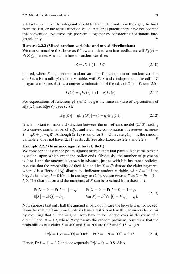
Example 2.2.5 (Liability insurance with a maximum coverage)Consider an insurance policy against a liability loss S. We want to determine theexpected value, the variance and the distribution function of the payment X on thispolicy, when there is a deductible of 100 and a maximum payment of 1000. In otherwords, if S≤ 100 then X = 0, if S≥ 1100 then X = 1000, otherwise X = S−100. Theprobability of a positive claim (S > 100) is 10% and the probability of a large loss(S ≥ 1100) is 2%. Given 100 < S < 1100, S has a uniform(100,1100) distribution.Again, we write X = IB where I denotes the number of payments, 0 or 1, and Brepresents the amount paid, if any. Therefore,

Pr[B = 1000 | I = 1] = 0.2;

Pr[B ∈ (x,x+dx) | I = 1] = c dx for 0 < x < 1000.(2.18)

Integrating the latter probability over x ∈ (0,1000) yields 0.8, so c = 0.0008.


0 1000

cArea = 0.8

Area = 0.2

Fig. 2.1 ‘Probability density function’ of B given I = 1 in Example 2.2.5.

The conditional distribution function of B, given I = 1, is neither discrete, norcontinuous. In Figure 2.1 we attempt to depict a pdf by representing the probabilitymass at 1000 by a bar of infinitesimal width and infinite height such that the areaequals 0.2. In actual fact we have plotted f (·), where f (x) = 0.0008 on (0,1000)and f (x) = 0.2/ε on (1000,1000+ ε) with ε > 0 very small.

For the cdf F of X we have

F(x) = Pr[X ≤ x] = Pr[IB≤ x]

= Pr[IB≤ x, I = 0]+Pr[IB≤ x, I = 1]

= Pr[IB≤ x | I = 0]Pr[I = 0]+Pr[IB≤ x | I = 1]Pr[I = 1]

(2.19)

which yields

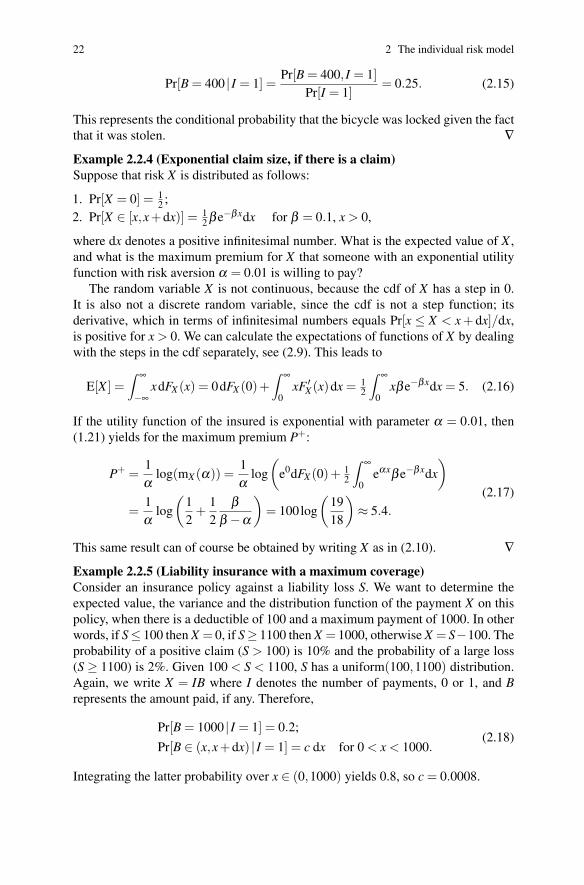
F(x) =

0×0.9+0×0.1 = 0 for x < 01×0.9+1×0.1 = 1 for x≥ 10001×0.9+ c x×0.1 for 0≤ x < 1000.

(2.20)

A graph of the cdf F is shown in Figure 2.2. For the differential (‘density’) of F , wehave

dF(x) =

0.9 for x = 00.02 for x = 10000 for x < 0 or x > 10000.00008 dx for 0 < x < 1000.

(2.21)

The moments of X can be calculated by using this differential. ∇

The variance of risks of the form IB can be calculated through the conditional dis-tribution of B, given I, by use of the well-known variance decomposition rule, see(2.7), which is also known as the law of total variance:


0 1000

.9

.981

Fig. 2.2 Cumulative distribution function F of X in Example 2.2.5.

Var[W ] = Var[E[W |V ]]+E[Var[W |V ]]. (2.22)

In statistics, the first term is the component of the variance of W , not explainedby knowledge of V ; the second is the explained component of the variance. Theconditional distribution of B | I = 0 is irrelevant, so for convenience, we let it beequal to the one of B | I = 1, meaning that we take I and B to be independent. Then,letting q = Pr[I = 1], µ = E[B] and σ2 = Var[B], we have E[X | I = 1] = µ andE[X | I = 0] = 0. Therefore, E[X | I = i] = µ i for both values i = 0,1, and analogously,Var[X | I = i] = σ2i. Hence,

E[X | I]≡ µI and Var[X | I]≡ σ2I, (2.23)

from which it follows that

E[X ] = E[E[X | I]] = E[µI] = µq;

Var[X ] = Var[E[X | I]]+E[Var[X | I]] = Var[µI]+E[σ2I]

= µ2q(1−q)+σ2q.

(2.24)

Notice that a continuous cdf F is not necessarily absolutely continuous in the senseof (2.3), as is demonstrated by the following example.

Example 2.2.6 ([♠] The Cantor cdf; continuous but not absolutely continuous)Let X1,X2, . . . be an infinite sequence of independent Bernoulli(1/2) random vari-ables. Define the following random variable:

W =∞

∑i=1

2Xi

3i =23

X1 +13

∞

∑i=1

2Xi+1

3i (2.25)

Then the possible values of W are, in the ternary system, 0.d1d2d3 . . . with di ∈{0,2} for all i = 1,2, . . . , and with di = 2 occurring if Xi = 1. Obviously, all of these

2.3 Convolution 25

values have zero probability as they correspond to all Xi having specific outcomes,so FW is continuous.

Also, all intervals of real numbers in (0,1) having a ternary digit di = 1 on someplace i = 1,2, . . . ,n are not possible values of W , hence FW is constant on the unionBn of all those intervals. But it is easy to see that the total length of these intervalstends to 1 as n→ ∞.

So we have constructed a continuous cdf FW , known as the Cantor distributionfunction, that is constant except on a set of length 0 (known as the Cantor set). Thecdf FW cannot be equal to the integral over its derivative, since this is zero almosteverywhere with respect to the Lebesgue measure (‘interval length’). So though FW

is continuous, it is not absolutely continuous as in (2.3). ∇

2.3 Convolution

In the individual risk model we are interested in the distribution of the total S of theclaims on a number of policies, with

S = X1 +X2 + · · ·+Xn, (2.26)

where Xi, i = 1,2, . . . ,n, denotes the payment on policy i. The risks Xi are assumedto be independent random variables. If this assumption is violated for some risks, forexample in case of fire insurance policies on different floors of the same building,then these risks could be combined into one term in (2.26).

The operation ‘convolution’ calculates the distribution function of X +Y from

FX+Y (s) = Pr[X +Y ≤ s]

=∫ ∞

−∞Pr[X +Y ≤ s |X = x]dFX (x)

=∫ ∞

−∞Pr[Y ≤ s− x |X = x]dFX (x)

=∫ ∞

−∞Pr[Y ≤ s− x]dFX (x)

=∫ ∞

−∞FY (s− x)dFX (x) =: FX ∗FY (s).

(2.27)

The cdf FX Y X Y

density function we use the same notation. If X and Y are discrete random variables,we find for the cdf of X +Y and the corresponding density

FX ∗FY (s) = ∑x

FY (s− x) fX (x) and fX ∗ fY (s) = ∑x

fY (s− x) fX (x), (2.28)

∗F (·) is called the convolution of the cdfs F (·) and F (·). For the

the cdfs of two independent random variables X and Y as follows:


where the sum is taken over all x with fX (x) > 0. If X and Y are continuous randomvariables, then

FX ∗FY (s) =∫ ∞

−∞FY (s− x) fX (x)dx (2.29)

and, taking the derivative under the integral sign to find the density,

fX ∗ fY (s) =∫ ∞

−∞fY (s− x) fX (x)dx. (2.30)

Since X +Y ≡Y +X , the convolution operator ∗ is commutative: FX ∗FY is identicalto FY ∗FX . Also, it is associative, since for the cdf of X +Y + Z, it does not matterin which order we do the convolutions, therefore

(FX ∗FY )∗FZ ≡ FX ∗ (FY ∗FZ)≡ FX ∗FY ∗FZ . (2.31)

For the sum of n independent and identically distributed random variables with mar-ginal cdf F , the cdf is the n-fold convolution power of F , which we write as

F ∗F ∗ · · · ∗F =: F∗n. (2.32)

Example 2.3.1 (Convolution of two uniform distributions)Suppose that X ∼ uniform(0,1) and Y ∼ uniform(0,2) are independent. What is thecdf of X +Y ?

The indicator function of a set A is defined as follows:

IA(x) =

{1 if x ∈ A0 if x /∈ A.

(2.33)

Indicator functions provide us with a concise notation for functions that are defineddifferently on some intervals. For all x, the cdf of X can be written as

FX (x) = xI[0,1)(x)+ I[1,∞)(x), (2.34)

while F ′Y (y) = 12 I[0,2)(y) for all y, which leads to the differential

dFY (y) = 12 I[0,2)(y)dy. (2.35)

The convolution formula (2.27), applied to Y +X rather than X +Y , then yields

FY+X (s) =∫ ∞

−∞FX (s− y)dFY (y) =

∫ 2

0FX (s− y) 1

2 dy, s≥ 0. (2.36)

The interval of interest is 0≤ s < 3. Subdividing it into [0,1), [1,2) and [2,3) yields

2.3 Convolution 27

FX+Y (s) =

{∫ s

0(s− y) 1

2 dy

}I[0,1)(s)

+

{∫ s−1

0

12 dy+

∫ s

s−1(s− y) 1

2 dy

}I[1,2)(s)

+

{∫ s−1

0

12 dy+

∫ 2

s−1(s− y) 1

2 dy

}I[2,3)(s)

= 14 s2I[0,1)(s)+ 1

4 (2s−1)I[1,2)(s)+ [1− 14 (3− s)2]I[2,3)(s).

(2.37)

Notice that X +Y is symmetric around s = 1.5. Although this problem could besolved graphically by calculating the probabilities by means of areas, see Exercise2.3.5, the above derivation provides an excellent illustration that, even in simplecases, convolution can be a laborious process. ∇

Example 2.3.2 (Convolution of discrete distributions)Let f1(x) = 1

4 , 12 , 1

4 for x = 0,1,2, f2(x) = 12 , 1

2 for x = 0,2 and f3(x) = 14 , 1

2 , 14 for

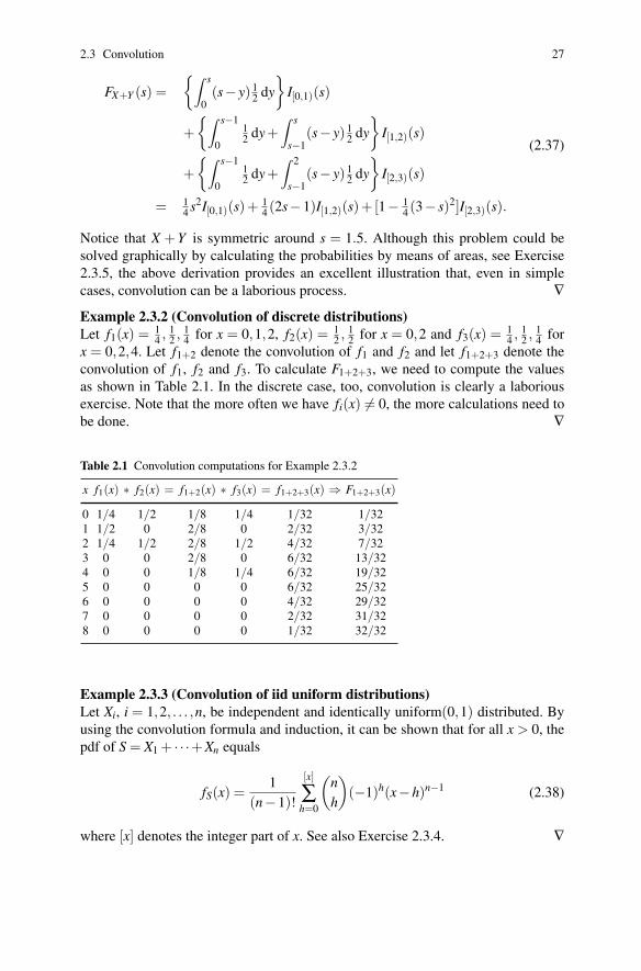
x = 0,2,4. Let f1+2 denote the convolution of f1 and f2 and let f1+2+3 denote theconvolution of f1, f2 and f3. To calculate F1+2+3, we need to compute the valuesas shown in Table 2.1. In the discrete case, too, convolution is clearly a laboriousexercise. Note that the more often we have fi(x) 6= 0, the more calculations need tobe done. ∇

Table 2.1 Convolution computations for Example 2.3.2

x f1(x) ∗ f2(x) = f1+2(x) ∗ f3(x) = f1+2+3(x) ⇒ F1+2+3(x)

0 1/4 1/2 1/8 1/4 1/32 1/321 1/2 0 2/8 0 2/32 3/322 1/4 1/2 2/8 1/2 4/32 7/323 0 0 2/8 0 6/32 13/324 0 0 1/8 1/4 6/32 19/325 0 0 0 0 6/32 25/326 0 0 0 0 4/32 29/327 0 0 0 0 2/32 31/328 0 0 0 0 1/32 32/32

Example 2.3.3 (Convolution of iid uniform distributions)Let Xi, i = 1,2, . . . ,n, be independent and identically uniform(0,1) distributed. Byusing the convolution formula and induction, it can be shown that for all x > 0, thepdf of S = X1 + · · ·+Xn equals

fS(x) =1

(n−1)!

[x]

∑h=0

(nh

)(−1)h(x−h)n−1 (2.38)

where [x] denotes the integer part of x. See also Exercise 2.3.4. ∇


Example 2.3.4 (Convolution of Poisson distributions)Let X ∼ Poisson(λ ) and Y ∼ Poisson(µ) be independent random variables. From(2.28) we have, for s = 0,1,2, . . .,

fX+Y (s) =s

∑x=0

fY (s− x) fX (x) =e−µ−λ

s!

s

∑x=0

(sx

)µs−xλ x

= e−(λ+µ) (λ + µ)s

s!,

(2.39)

where the last equality is the binomial theorem. Hence, X +Y is Poisson(λ + µ)distributed. For a different proof, see Exercise 2.4.2. ∇

2.4 Transforms

mX (t) = E[etX , −∞ < t < h, (2.40)

exponential moments E[eεx] for some ε > 0 exist.

mX+Y (t) = E[et(X+Y )

]= E

[etX]E

[etY = mX (t)mY (2.41)

φX (t) = E[eitX]= E

[cos(tX)+ i sin(tX)

], −∞ < t < ∞. (2.42)

bers, although applying the same function formula derived for real t to imaginary tas well produces the correct results most of the time, resulting for example in the

2 2 2

istic function.As their name indicates, moment generating functions can be used to generate

moments of random variables. The usual series expansion of ex yields

be made easier by using transforms of the cdf. The moment generating function

]

]

does not exist. The characteristic function, however, always exists. It is defined as:

Determining the distribution of the sum of independent random variables can often

So, the convolution of cdfs corresponds to simply multiplying the mgfs. Note that

for some h. The mgf is going to be used especially in an interval around 0, which

(t).

the mgf-transform is one-to-one, so every cdf has exactly one mgf. Also, it is con-

If X and Y are independent, then

mgfs. See Exercises 2.4.12 and 2.4.13.For random variables with a heavy tail, such as the Pareto distributions, the mgf

requires h > 0 to hold. Note that this is the case only for light-tailed risks, of which

N(0,2) distribution with mgf exp(t ) having exp((it) ) = exp(−t ) as its character-

A disadvantage of the characteristic function is the need to work with complex num-

tinuous, in the sense that the mgf of the limit of a series of cdfs is the limit of the

(mgf) suits our purposes best. For a non-negative random variable X , it is defined as

2.4 Transforms 29

mX (t) = E[etX ] =∞

∑k=0

E[Xk]tk

k!, (2.43)

so the k-th moment of X equals

k dk

dtk X (t)

∣∣∣∣t=0

. (2.44)

Moments can also be generated from the characteristic function in similar fashion.

natural numbers as values:

gX (t) = E[tX∞

∑k=0

tk Pr[X = k]. (2.45)

central moment; it is defined as:

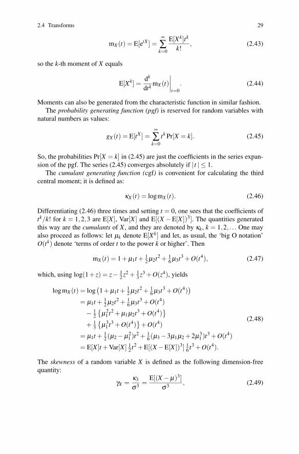
κX (t) = logmX (t). (2.46)

tk/k! for k = 1,2,3 are E[X ], Var[X ] and E[(X −E[X ])3]. The quantities generatedthis way are the cumulants of X , and they are denoted by κk, k = 1,2, . . . One mayalso proceed as follows: let µk denote E[Xk] and let, as usual, the ‘big O notation’

k

mX (t) = 1+ µ1t + 12 µ2t2 + 1

6 µ3t3 +O(t4), (2.47)

which, using log(1+ z) = z− 12 z2 + 1

3 z3 +O(z4), yields

logmX (t) = log(1+ µ1t + 1

2 µ2t2 + 16 µ3t3 +O(t4)

)

= µ1t + 12 µ2t2 + 1

6 µ3t3 +O(t4)

− 12

{µ2

1 t2 + µ1µ2t3 +O(t4)}

+ 13

{µ3

1 t3 +O(t4)}

+O(t4)

= µ1t + 12 (µ2−µ2

1 )t2 + 16 (µ3−3µ1µ2 +2µ3

1 )t3 +O(t4)

= E[X ]t +Var[X ] 12 t2 +E[(X−E[X ])3] 1

6 t3 +O(t4).

(2.48)

The skewness of a random variable X is defined as the following dimension-freequantity:

γX =κ3

σ3 =E[(X−µ)3]

σ3 , (2.49)

Differentiating (2.46) three times and setting t = 0, one sees that the coefficients of

mE[X ] =

The probability generating function (pgf) is reserved for random variables with

sion of the pgf. The series (2.45) converges absolutely if | t | ≤ 1.

] =

O(t ) denote ‘terms of order t to the power k or higher’. Then

The cumulant generating function (cgf) is convenient for calculating the third

So, the probabilities Pr[X = k] in (2.45) are just the coefficients in the series expan-


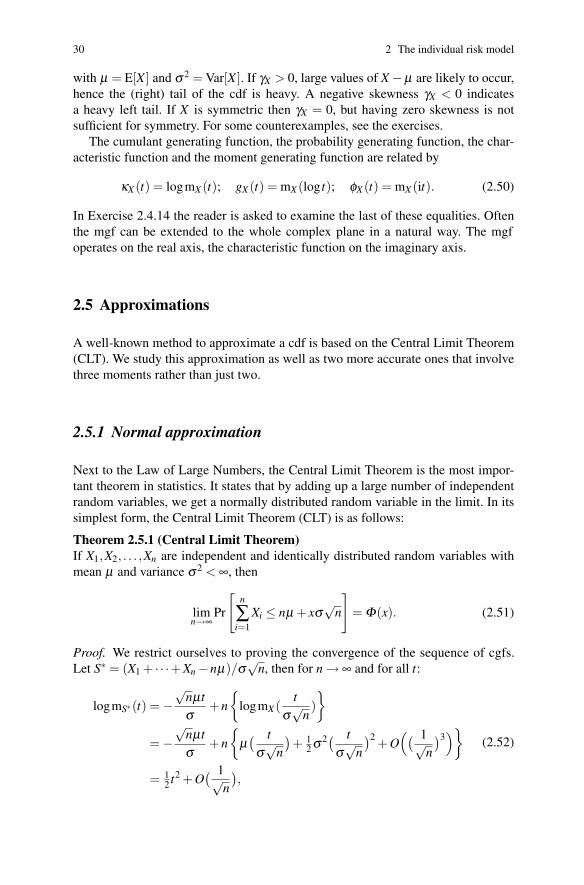
with µ = E[X ] and σ2 = Var[X ]. If γX > 0, large values of X−µ are likely to occur,hence the (right) tail of the cdf is heavy. A negative skewness γX < 0 indicatesa heavy left tail. If X is symmetric then γX = 0, but having zero skewness is notsufficient for symmetry. For some counterexamples, see the exercises.

acteristic function and the moment generating function are related by

κX (t) = logm (t); g (t) = mX (log t); φX (t) = mX (2.50)

In Exercise 2.4.14 the reader is asked to examine the last of these equalities. Often

operates on the real axis, the characteristic function on the imaginary axis.

2.5 Approximations

A well-known method to approximate a cdf is based on the Central Limit Theorem(CLT). We study this approximation as well as two more accurate ones that involvethree moments rather than just two.

2.5.1 Normal approximation

Next to the Law of Large Numbers, the Central Limit Theorem is the most impor-tant theorem in statistics. It states that by adding up a large number of independent

Theorem 2.5.1 (Central Limit Theorem)If X1,X2, . . . ,Xn are independent and identically distributed random variables withmean µ and variance σ2 < ∞, then

limn→∞

Pr

[n

∑i=1

Xi ≤ nµ + xσ√

n

]= Φ(x). (2.51)

Let S∗ = (X1 + · · ·+Xn−nµ)/σ√

n, then for n→ ∞ and for all t:

logmS∗(t) =−√

nµtσ

+n

{logmX (

tσ√

n)

}

=−√

nµtσ

+n

{µ( t

σ√

n

)+ 1

2 σ2( tσ√

n

)2+O

(( 1√n

)3)}

= 12 t2 +O

( 1√n

),

(2.52)

X (it).

The cumulant generating function, the probability generating function, the char-

the mgf can be extended to the whole complex plane in a natural way. The mgf

X

simplest form, the Central Limit Theorem (CLT) is as follows:

Proof.

random variables, we get a normally distributed random variable in the limit. In its

We restrict ourselves to proving the convergence of the sequence of cgfs.

2.5 Approximations 31

12 t2). As a

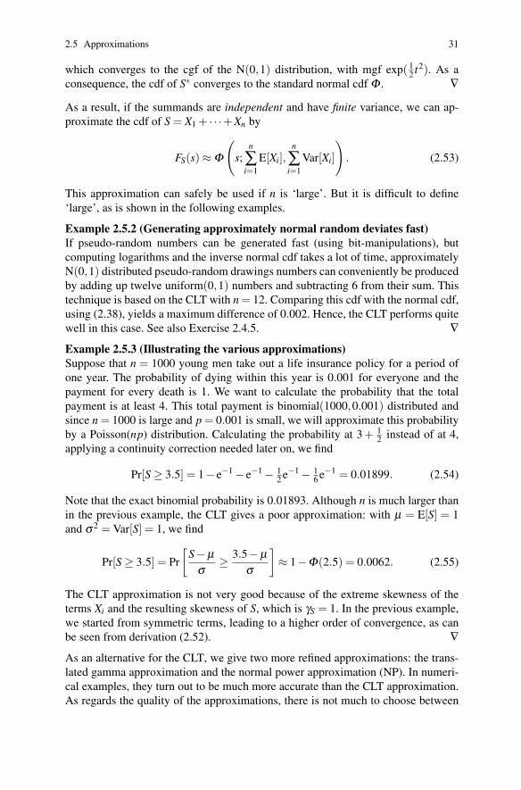
consequence, the cdf of S∗ ∇

As a result, if the summands are independent and have finite variance, we can ap-proximate the cdf of S = X1 + · · ·+Xn by

FS(s)≈Φ

(s;

n

∑i=1

E[Xi],n

∑i=1

Var[Xi]

). (2.53)

‘large’, as is shown in the following examples.

Example 2.5.2 (Generating approximately normal random deviates fast)If pseudo-random numbers can be generated fast (using bit-manipulations), but

N(0,1) distributed pseudo-random drawings numbers can conveniently be producedby adding up twelve uniform(0,1) numbers and subtracting 6 from their sum. Thistechnique is based on the CLT with n = 12. Comparing this cdf with the normal cdf,using (2.38), yields a maximum difference of 0.002. Hence, the CLT performs quitewell in this case. See also Exercise 2.4.5. ∇

Example 2.5.3 (Illustrating the various approximations)Suppose that n = 1000 young men take out a life insurance policy for a period ofone year. The probability of dying within this year is 0.001 for everyone and thepayment for every death is 1. We want to calculate the probability that the totalpayment is at least 4. This total payment is binomial(1000,0.001) distributed andsince n = 1000 is large and p = 0.001 is small, we will approximate this probabilityby a Poisson(np) distribution. Calculating the probability at 3 + 1

2 instead of at 4,applying a continuity correction needed later on, we find

Pr[S≥ 3.5] = 1− e−1− e−1− 12 e−1− 1 e−1 = 0.01899. (2.54)

Note that the exact binomial probability is 0.01893. Although n is much larger thanin the previous example, the CLT gives a poor approximation: with µ = E[S] = 1and σ2 = Var[S] = 1, we find

Pr[S≥ 3.5] = Pr

[S−µ

σ≥ 3.5−µ

σ

]≈ 1−Φ(2.5) = 0.0062. (2.55)

The CLT approximation is not very good because of the extreme skewness of theterms Xi and the resulting skewness of S, which is γS = 1. In the previous example,we started from symmetric terms, leading to a higher order of convergence, as canbe seen from derivation (2.52). ∇

As an alternative for the CLT, we give two more refined approximations: the trans-lated gamma approximation and the normal power approximation (NP). In numeri-cal examples, they turn out to be much more accurate than the CLT approximation.As regards the quality of the approximations, there is not much to choose between

This approximation can safely be used if n is ‘large’. But it is difficult to define

converges to the standard normal cdf Φ .which converges to the cgf of the N(0,1) distribution, with mgf exp(

computing logarithms and the inverse normal cdf takes a lot of time, approximately

6


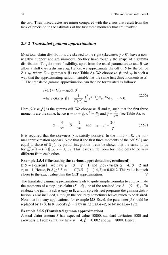
the two. Their inaccuracies are minor compared with the errors that result from thelack of precision in the estimates of the first three moments that are involved.

2.5.2 Translated gamma approximation

Most total claim distributions are skewed to the right (skewness γ > 0), have a non-negative support and are unimodal. So they have roughly the shape of a gammadistribution. To gain more flexibility, apart from the usual parameters α and β weallow a shift over a distance x0. Hence, we approximate the cdf of S by the cdf of

0 0 in such away that the approximating random variable has the same first three moments as S.

The translated gamma approximation can then be formulated as follows:

FS(s)≈ G(s− x0;α,β ),

where G(x;α,β ) =1

Γ (α)

∫ x

0yα−1β α e−βydy, x≥ 0.

(2.56)

Here G(x;α,β ) is the gamma cdf. We choose α , β and x0 such that the first threemoments are the same, hence µ = x0 + α

β , σ2 = αβ 2 and γ = 2√

α (see Table A), so

α =4γ2 , β =

2γσ

and x0 = µ− 2σγ

. (2.57)

mal approximation appears. Note that if the first three moments of the cdf F(·) areequal to those of G(·), by partial integration it can be shown that the same holdsfor

∫ ∞0

j

different from each other.

Example 2.5.4 (Illustrating the various approximations, continued)If S ∼ Poisson(1), we have µ = σ = γ = 1, and (2.57) yields α = 4, β = 2 andx0 =−1. Hence, Pr[S≥ 3.5]≈ 1−G(3.5−(−1);4,2) = 0.0212. This value is muchcloser to the exact value than the CLT approximation. ∇

The translated gamma approximation leads to quite simple formulas to approximatethe moments of a stop-loss claim (S− d)+ or of the retained loss S− (S− d)+. Toevaluate the gamma cdf is easy in R, and in spreadsheet programs the gamma distri-bution is also included, although the accuracy sometimes leaves much to be desired.Note that in many applications, for example MS Excel, the parameter β should bereplaced by 1/β . In R, specify β = 2 by using rate=2, or by scale=1/2.

Example 2.5.5 (Translated gamma approximation)A total claim amount S has expected value 10000, standard deviation 1000 andskewness 1. From (2.57) we have α = 4, β = 0.002 and x0 = 8000. Hence,

It is required that the skewness γ is strictly positive. In the limit γ ↓ 0, the nor-

x [1−F(x)]dx, j = 0,1,2. This leaves little room for these cdfs to be very

Z + x , where Z ∼ gamma(α,β ) (see Table A). We choose α , β and x

2.5 Approximations 33

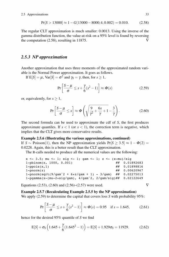
Pr[S > 13000]≈ 1−G(13000−8000;4,0.002) = 0.010. (2.58)

The regular CLT approximation is much smaller: 0.0013. Using the inverse of thegamma distribution function, the value-at-risk on a 95% level is found by reversingthe computation (2.58), resulting in 11875. ∇

2.5.3 NP approximation

Another approximation that uses three moments of the approximated random vari-able is the Normal Power approximation. It goes as follows.

If E[S] = µ , Var[S] = σ2 and γS = γ , then, for s≥ 1,

Pr

[S−µ

σ≤ s+

γ6(s2−1)

]≈Φ(s) (2.59)

or, equivalently, for x≥ 1,

Pr

[S−µ

σ≤ x

]≈Φ

(√9γ2 +

6xγ

+1− 3γ

). (2.60)

The second formula can be used to approximate the cdf of S, the first producesapproximate quantiles. If s < 1 (or x < 1), the correction term is negative, whichimplies that the CLT gives more conservative results.

Example 2.5.6 (Illustrating the various approximations, continued)If S ∼ Poisson(1), then the NP approximation yields Pr[S ≥ 3.5] ≈ 1−Φ(2) =0.0228. Again, this is a better result than the CLT approximation.

The R-calls needed to produce all the numerical values are the following:

x <- 3.5; mu <- 1; sig <- 1; gam <- 1; z <- (x-mu)/sig1-pbinom(x, 1000, 0.001) ## 0.018926831-ppois(x,1) ## 0.018988161-pnorm(z) ## 0.006209671-pnorm(sqrt(9/gamˆ2 + 6*z/gam + 1) - 3/gam) ## 0.022750131-pgamma(x-(mu-2*sig/gam), 4/gamˆ2, 2/gam/sig)## 0.02122649

Equations (2.53), (2.60) and (2.56)–(2.57) were used. ∇

Example 2.5.7 (Recalculating Example 2.5.5 by the NP approximation)We apply (2.59) to determine the capital that covers loss S with probability 95%:

Pr

[S−µ

σ≤ s+

γ6(s2−1)

]≈Φ(s) = 0.95 if s = 1.645, (2.61)

hence for the desired 95% quantile of S we find

E[S]+σS

(1.645+

γ6(1.6452−1)

)= E[S]+1.929σS = 11929. (2.62)


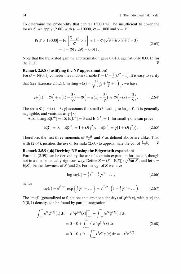
To determine the probability that capital 13000 will be insufficient to cover thelosses S, we apply (2.60) with µ = 10000, σ = 1000 and γ = 1:

Pr[S > 13000] = Pr

[S−µ

σ> 3

]≈ 1−Φ(

√9+6×3+1−3)

= 1−Φ(2.29) = 0.011.

(2.63)

Note that the translated gamma approximation gave 0.010, against only 0.0013 forthe CLT. ∇

Remark 2.5.8 (Justifying the NP approximation)For U ∼N(0,1) consider the random variable Y =U + γ

6 (U2−1). It is easy to verify

that (see Exercise 2.5.21), writing w(x) =

√(9γ2 + 6x

γ +1)

+, we have

FY (x) = Φ(

+w(x)− 3γ

)−Φ

(−w(x)− 3

γ

)≈Φ

(w(x)− 3

γ

). (2.64)

The term Φ(−w(x)− 3/γ) accounts for small U leading to large Y . It is generallynegligible, and vanishes as γ ↓ 0.

Also, using E[U6] = 15, E[U4] = 3 and E[U2] = 1, for small γ one can prove

E[Y ] = 0; E[Y 2] = 1+O(γ2); E[Y 3] = γ(1+O(γ2)

). (2.65)

S−µσ

with (2.64), justifies the use of formula (2.60) to approximate the cdf of S−µσ . ∇

Remark 2.5.9 ([♠] Deriving NP using the Edgeworth expansion)Formula (2.59) can be derived by the use of a certain expansion for the cdf, though√

Var[S], and let γ =3

logmZ(t) = 12 t2 + 1

6 γt3 + . . . , (2.66)

hencemZ(t) = et2/2 · exp

{16 γt3 + . . .

}= et2/2 ·

(1+ 1

6 γt3 + . . .). (2.67)

(3)(x), with ϕ(x) theN(0,1) density, can be found by partial integration:

∫ ∞

−∞etxϕ(3)(x)dx = etxϕ(2)(x)

∣∣∣∞

−∞−∫ ∞

−∞tetxϕ(2)(x)dx

= 0−0+∫ ∞

−∞t2etxϕ(1)(x)dx

= 0−0+0−∫ ∞

−∞t3etxϕ(x)dx =−t3et2/2.

(2.68)

Therefore, the first three moments of and Y as defined above are alike. This,

The ‘mgf’ (generalized to functions that are not a density) of ϕ

not in a mathematically rigorous way. Define Z = (S−E[S])/E[Z ] be the skewness of S (and Z). For the cgf of Z we have

2.6 Application: optimal reinsurance 35

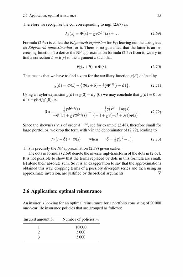
FZ(x) = Φ(x)− 16 γΦ (3)(x)+ . . . (2.69)

Z

find a correction δ = δ (s) to the argument s such that

FZ(s+δ )≈Φ(s). (2.70)

That means that we have to find a zero for the auxiliary function g(δ ) defined by

g(δ ) = Φ(s)−{

Φ(s+δ )− 16 γΦ (3)(s+δ )

}. (2.71)

′

δ ≈−g(0)/g′(0), so

δ ≈ − 16 γΦ (3)(s)

−Φ ′(s)+ 16 γΦ (4)(s)

=− 1

6 γ(s2−1)ϕ(s)(−1+ 1

6 γ(−s3 +3s))ϕ(s)

. (2.72)

Since the skewness γ is of order λ−1/2, see for example (2.48), therefore small forlarge portfolios, we drop the term with γ in the denominator of (2.72), leading to

FZ(s+δ )≈Φ(s) when δ = 16 γ(s2−1). (2.73)

This is precisely the NP approximation (2.59) given earlier.

It is not possible to show that the terms replaced by dots in this formula are small,let alone their absolute sum. So it is an exaggeration to say that the approximations

approximate inversion, are justified by theoretical arguments. ∇

2.6 Application: optimal reinsurance

An insurer is looking for an optimal reinsurance for a portfolio consisting of 20000one-year life insurance policies that are grouped as follows:

Insured amount bk Number of policies nk

1 10 0002 5 0003 5 000

Using a Taylor expansion g(δ )≈ g(0)+δg (0) we may conclude that g(δ ) = 0 for

Formula (2.69) is called the Edgeworth expansion for F ; leaving out the dots gives

creasing function. To derive the NP approximation formula (2.59) from it, we try to

Therefore we recognize the cdf corresponding to mgf (2.67) as:

an Edgeworth approximation for it. There is no guarantee that the latter is an in-

obtained this way, dropping terms of a possibly divergent series and then using an

The dots in formula (2.69) denote the inverse mgf-transform of the dots in (2.67).


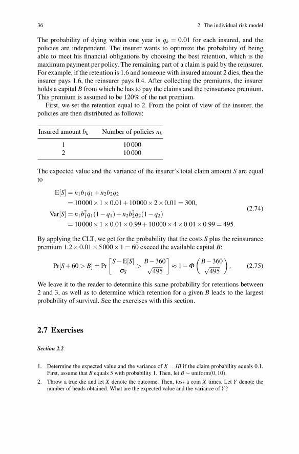
The probability of dying within one year is qk = 0.01 for each insured, and thepolicies are independent. The insurer wants to optimize the probability of beingable to meet his financial obligations by choosing the best retention, which is themaximum payment per policy. The remaining part of a claim is paid by the reinsurer.For example, if the retention is 1.6 and someone with insured amount 2 dies, then theinsurer pays 1.6, the reinsurer pays 0.4. After collecting the premiums, the insurerholds a capital B from which he has to pay the claims and the reinsurance premium.This premium is assumed to be 120% of the net premium.

First, we set the retention equal to 2. From the point of view of the insurer, thepolicies are then distributed as follows:

Insured amount bk Number of policies nk

1 10 0002 10 000

The expected value and the variance of the insurer’s total claim amount S are equalto

E[S] = n1b1q1 +n2b2q2

= 10000×1×0.01+10000×2×0.01 = 300,

Var[S] = n1b21q1(1−q1)+n2b2

2q2(1−q2)

= 10000×1×0.01×0.99+10000×4×0.01×0.99 = 495.

(2.74)

By applying the CLT, we get for the probability that the costs S plus the reinsurancepremium 1.2×0.01×5000×1 = 60 exceed the available capital B:

Pr[S +60 > B] = Pr

[S−E[S]

σS>

B−360√495

]≈ 1−Φ

(B−360√

495

). (2.75)

We leave it to the reader to determine this same probability for retentions between2 and 3, as well as to determine which retention for a given B leads to the largestprobability of survival. See the exercises with this section.

2.7 Exercises

Section 2.2

1. Determine the expected value and the variance of X = IB if the claim probability equals 0.1.First, assume that B equals 5 with probability 1. Then, let B∼ uniform(0,10).

2. Throw a true die and let X denote the outcome. Then, toss a coin X times. Let Y denote thenumber of heads obtained. What are the expected value and the variance of Y ?

2.7 Exercises 37

3. In Example 2.2.4, plot the cdf of X . Also determine, with the help of the obtained differential,the premium the insured is willing to pay for being insured against an inflated loss 1.1X . Dothe same by writing X = IB. Has the zero utility premium followed inflation exactly?

4. Calculate E[X ], Var[X ] and the moment generating function mX (t) in Example 2.2.5 with thehelp of the differential. Also plot the ‘density’.

5. If X = IB, what is mX (t)?

6. Consider the following cdf F : F(x) =

0 for x < 2,x4 for 2≤ x < 4,1 for 4≤ x.

Determine independent random variables I, X and Y such that Z = IX +(1− I)Y has cdf F ,I ∼ Bernoulli, X is a discrete and Y a continuous random variable.

7. The differential of cdf F is dF(x) =

dx/3 for 0 < x < 1 and 2 < x < 3,16 for x ∈ {1,2},0 elsewhere.

Find a discrete cdf G, a continuous cdf H and a real constant c with the property that F(x) =cG(x)+(1− c)H(x) for all x.

8.independent. Compare E[T k] with E[Zk], k = 1,2.

9. In the previous exercise, assume additionally that X and Y are independent N(0,1). Whatdistributions do T and Z have?

10. [♠] In Example 2.2.6, show that E[W ] = 12 and Var[W ] = 1

8 .Also show that mW (t) = et/2 ∏∞

i=1 cosh(t/3i). Recall that cosh(t) = (et + e−t)/2.

Section 2.3

1. Calculate Pr[S = s] for s = 0,1, . . . ,6 when S = X1 +2X2 +3X3 and Xj ∼ Poisson( j).

2. Determine the number of multiplications of non-zero numbers that are needed for the calcula-tion of all probabilities f1+2+3(x) in Example 2.3.2. How many multiplications are needed tocalculate F1+···+n(x), x = 0, . . . ,4n−4 if fk = f3 for k = 4, . . . ,n?

3.

4. [♠] Verify the expression (2.38) in Example 2.3.3 for n = 1,2,3 by using convolution. Deter-S

5. Assume that X ∼ uniform(0,3) and Y ∼ uniform(−1,1). Calculate FX+Y (z) graphically by

Section 2.4

1. 1 +X2 where the Xk are independent and exponential(k) distributed.

density using the method of partial fractions.

2.

3. What is the fourth cumulant κ4 in terms of the central moments?

Determine the cdf of S = XDo this both by convolution and by calculating the mgf and identifying the corresponding

mine F (x) for these values of n. Using induction, verify (2.38) for arbitrary n.

Same as Example 2.3.4, but now by making use of the mgfs.

using the area of the sets {(x,y) |x+ y≤ z,x ∈ (0,3) and y ∈ (−1,1)}.

has a normal distribution.

Suppose that T = qX +(1−q)Y and Z = IX +(1− I)Y with I ∼ Bernoulli(q) and I, X and Y

Prove by convolution that the sum of two independent normal random variables, see Table A,


4. Prove that cumulants actually cumulate in the following sense: if X and Y are independent,

5. Prove that the sum of twelve independent uniform(0,1) random variables has variance 1 andexpected value 6. Determine κ3 and κ4.Plot the difference between the cdf of this random variable and the N(6,1) cdf, using theexpression for FS(x) found in Exercise 2.3.4.

6.

7. Determine the skewness of a gamma(α,β ) distribution.

8. If S is symmetric, then γS = 0. this, but also, for S = X1 + X2 + X3 with X1 ∼Bernoulli(0.4), X2 ∼ Bernoulli(0.7) and X3 ∼ Bernoulli(p), all independent, calculate the value

S

9. Determine the skewness of a risk of the form Ib where I∼ Bernoulli(q) and b is a fixed amount.

actually symmetric?

Table A.

and gamma.

1 2 i

i

for all x.

14. Examine the equality φX (t) = mX

For which values of p is Z symmetric?

16. For which values of δ is the skewness of X − δY equal to 0, if X ∼ gamma(2,1) and Y ∼exponential(1)?

valued random variable be used to generate probabilities?

Section 2.5

1. What happens if we replace the argument 3.5 in Example 2.5.3 by 3−0, 3+0, 4−0 and 4+0?Is a correction for continuity needed here?

2. Prove that both versions of the NP approximation are equivalent.

3. If Y ∼ gamma(α,β ) and γY = 2√α ≤ 4, then

√4βY −

√4α−1

≈∼ N(0,1). See ex. 2.5.14 fora comparison of the first four moments. So approximating a translated gamma approximationwith parameters α , β and x0, we also have Pr[S≤ s]≈Φ

(√4β (s− x0)−

√4α−1

).

Show Pr[S≤ s]≈Φ(√

8γ

s−µσ + 16

γ2 −√

16γ2 −1

)if α = 4

γ2 ,β = 2γσ ,x0 = µ− 2σ

γ .

Inversely, show Pr[S≤ x0 + 1

4β (y+√

4α−1)2]≈ 1− ε if Φ(y) = 1− ε ,

as well as Pr[ S−µ

σ ≤ y+ γ8 (y2−1)+ y(

√1− γ2/16−1)

]≈Φ(y).

Show that the characteristic function is real-valued if X is symmetric around 0.

13. Show that X and Y are equal in distribution if they have the same support {0,δ ,2δ , . . . ,nδ}

Prove

Determine the skewness of a Poisson(µ) distribution.

10. Determine the pgf of the binomial, the Poisson and the negative binomial distribution, see

11. Determine the cgf and the cumulants of the following distributions: Poisson, binomial, normal

= 0, and verify that S is not symmetric.

then the kth cumulant of X +Y equals the sum of the kth cumulants of X and Y .

converge to the pgf of Y for each argument t when i→∞, verify that also Pr[X = x]→ Pr[Y = x]

For which values of q and b is the skewness equal to zero, and for which of these values is I

for some δ > 0 and moreover, they have the same mgf.

the same pgf. If X ,X , . . . are risks, again with range {0,1, . . . ,n}, such that the pgfs of X

15. Show that the skewness of Z = X + 2Y is 0 if X ∼ binomial(8, p) and Y ∼ Bernoulli(1− p).

(it) from (2.50), for the special case that X ∼ exponential(1).

17. Can the pgf of a random variable be used to generate moments? Can the mgf of an integer-

12. Show that X and Y are equal in distribution if they have the same support {0,1, . . . ,n} and

of p such that S has skewness γ

2.7 Exercises 39

4. Show that the translated gamma approximation as well as the NP approximation result in thenormal approximation (CLT) if µ and σ2 are fixed and γ ↓ 0.

5. Approximate the critical values of a χ218 distribution for ε = 0.05,0.1,0.5,0.9,0.95 with the

NP approximation and compare the results with the exact values.

6. In the previous exercise, what is the result if the translated gamma approximation is used?

7. Use the identity ‘having to wait longer than x for the nth event’ ≡ ‘at most n−1 events occurin (0,x)’ in a Poisson process to prove that Pr[Z > x] = Pr[N < n] if Z ∼ gamma(n,1) and N ∼Poisson(x). How can this fact be used to calculate the translated gamma approximation?

8. Compare the exact critical values of a χ218 distribution for ε = 0.05,0.1,0.5,0.9,0.95 with the

approximations obtained in exercise 2.5.3.

9. An insurer’s portfolio contains 2 000 one-year life insurance policies. Half of them are charac-terized by a payment b1 = 1 and a probability of dying within 1 year of q1 = 1%. For the otherhalf, we have b2 = 2 and q2 = 5%. Use the CLT to determine the minimum safety loading, as apercentage, to be added to the net premium to ensure that the probability that the total paymentexceeds the total premium income is at most 5%.

10. As the previous exercise, but now using the NP approximation. Employ the fact that the third

11. Show that the right hand side of (2.60) is well-defined for all x ≥−1. What are the minimumand the maximum values? Is the function increasing? What happens if x = 1?

12. Suppose that X has expected value µ = 1000 and standard deviation σ = 2000. Determinethe skewness γ if (i) X is normal, (ii) X/φ ∼ Poisson(µ/φ ), (iii) X ∼ gamma(α,β ), (iv) X ∼inverse Gaussian(α,β ) or (v) X ∼ lognormal(ν ,τ2). Show that the skewness is infinite if (vi)X ∼ Pareto. See also Table A.

13. A portfolio consists of two types of contracts. For type k, k = 1,2, the claim probability is qkand the number of policies is nk. If there is a claim, then its size is x with probability pk(x):

nk q pk(1) pk(2) pk(3)

Type 1 1000 0.01 0.5 0 0.5Type 2 2000 0.02 0.5 0.5 0

Assume that the contracts are independent. Let Sk denote the total claim amount of the con-tracts of type k and let S = S1 +S2. Calculate the expected value and the variance of a contractof type k, k = 1,2. Then, calculate the expected value and the variance of S. Use the CLT todetermine the minimum capital that covers all claims with probability 95%.

14. [♠] Let U ∼ gamma(α,1), Y ∼ N(√

4α−1,1) and T =√

4U . Show that E[Ut ] = Γ (α +t)/Γ (α), t > 0. Then show that E[Y j] ≈ E[T j], j = 1,3, by applying Γ (α + 1/2)/Γ (α) ≈√

α−1/4 and αΓ (α) = Γ (α +1). Also, show that E[Y 2] = E[T 2] and E[Y 4] = E[T 4]−2.

15. [♠] A justification for the ‘correction for continuity’, see Example 2.5.3, used to approximate

continuous cdf of some non-negative random variable, and construct cdf H by H(k + ε) =G(k + 0.5),k = 0,1,2, . . . ,0 ≤ ε < 1. Using the midpoint rule with intervals of length 1 toapproximate the right hand side of (1.33) at d = 0, show that the means of G and H are aboutequal. Conclude that if G is a continuous cdf that is a plausible candidate for approximatingthe discrete cdf F and has the same mean as F , by taking F(x) := G(x + 0.5) one gets anapproximation with the proper mean value. [Taking F(x) = G(x) instead, one gets a mean thatis about µ + 0.5 instead of µ . Thus very roughly speaking, each tail probability of the sumapproximating (1.33) will be too big by a factor 1

2µ .]

16. To get a feel for the approximation error as opposed to the error caused by errors in the esti-mates of µ , σ and γ needed for the NP approximation and the gamma approximation, recal-

k

cdfs of integer valued random variables by continuous ones, goes as follows. Let G be the

cumulant of the total payment equals the sum of the third cumulants of the risks.


culate Example 2.5.5 if the following parameters are changed: (i) µ = 10100 (ii) σ = 1020(iii) µ = 10100 and σ = 1020 (iv) γ = 1.03. Assume that the remaining parameters are as theywere in Example 2.5.5.

17. The function pNormalPower, when implemented carelessly, sometimes produces the valueNaN (not a number). Why and when could that happen? Build in a test to cope with this

ution using the calls pTransGam(0:10,1,1,1) and ppois(0:10,1).To see the effect of applying a correction for continuity, compare also with the result ofpTransGam(0:10+0.5,1,1,1).

19. Repeat the previous exercise, but now for the Normal Power approximation.

quantile functions qTransGam and qNormalPower, and do some testing.

21. Prove (2.64) and (2.65).

Section 2.6

1. In the situation of Section 2.6, calculate the probability that B will be insufficient for retentionsd ∈ [2,3]. Give numerical results for d = 2 and d = 3 if B = 405.

2. Determine the retention d ∈ [2,3] that minimizes this probability for B = 405. Which retentionis optimal if B = 404?

3. Calculate the probability that B will be insufficient if d = 2 by using the NP approximation.

18. Compare the results of the translated gamma approximation with an exact Poisson(1) distrib-

situation more elegantly.

20. Note that we have prefixed the (approximate) cdfs with p, as is customary in R. Now write

Modern Actuarial Risk Theory - ReadingSample - NET

Documents