Models of Nondeterministic Regular Expressions

Journal of Computer and System Sciences 59, 412�449 (1999)

Models of Nondeterministic Regular Expressions1

Flavio Corradini

Dip. di Mat. Pura ed Appl., Universita� dell 'Aquila, L'Aquila, ItalyE-mail: flavio�univaq.it

Rocco De Nicola2

Dip. di Sistemi e Informatica, Universita� di Firenze, Florence, ItalyE-mail: denicola�dsi.unifi.it

and

Anna Labella

Dip. di Scienze dell'Informazione, Universita� di Roma ``La Sapienza,'' Rome, ItalyE-mail: labella�dsi.uniroma1.it

Received October 21, 1996; revised March 15, 1999

Nondeterminism is a direct outcome of interactions and is, therefore a cen-tral ingredient for modelling concurrent systems. Trees are very useful formodelling nondeterministic behaviour. We aim at a tree-based interpretationof regular expressions and study the effect of removing the idempotence lawX+X=X and the distribution law X v (Y+Z)=X vY+X vZ from Kleenealgebras. We show that the free model of the new set of axioms is a class oftrees labelled over A. We also equip regular expressions with a two-levelbehavioural semantics. The basic level is described in terms of a class oflabelled transition systems that are detailed enough to describe the numberof equal actions a system can perform from a given state. The abstract levelis based on a so-called resource bisimulation preorder that permits ignoringuninteresting details of transition systems. The three proposed interpretationsof regular expressions (algebraic, denotational, and behavioural ) are proven tocoincide. When dealing with infinite behaviours, we rely on a simple versionof the |-induction and obtain a complete proof system also for the fulllanguage of nondeterministic regular expressions. � 1999 Academic Press

Article ID jcss.1999.1636, available online at http:��www.idealibrary.com on

4120022-0000�99 �30.00Copyright � 1999 by Academic PressAll rights of reproduction in any form reserved.

1 This work has been partially founded by EEC within the HCM Project EXPRESS, and by CNRwithin the project ``Specifica ad Alto Livello e Verifica di Sistemi Digitali.''

2 Corresponding author.

1. INTRODUCTION

The theory of regular languages was first studied by Kleene [23] and thenaxiomatized by Salomaa [30] to obtain so-called Kleene algebras. These arealgebraic structures with +, v , *, 0, and 1 operators satisfying certain properties(the reader is referred to Table 1 for a first sample) that have been fruitfully usedalso in many areas of computer science.

Building on an alphabet A, regular expressions can be defined via the syntaxbelow:

P ::=0 | 1 | a | P+P | P vP | P*, where a is in A.

We will refer to the set of terms generated by this BNF as PL, for process language.Recently a new axiomatization of Kleene algebras has been proposed by Kozen

[25] (see also [6]), that relies on the original axiomatization of Table 1 proposedin [30] for finite (*-free) terms, and on the laws of Table 2 for infinite expressions.There, � stands for the partial order obtained by asserting X�X+Y and theaxioms in Table 1 and by requiring preservation by v and +.

Regular expressions and Kleene algebras have also been a direct inspiration formany of the constructs and axiomatizations of concurrency models such as CCS,CSP, and ACP (see, e.g., [9, 22, 27]), generally referred to as process algebras. Ifone considers PL as defined above, it is possible to interpret its operator symbolsin terms of basic agents and operators for agents composition. Thus 0 can be seenas the zero agent introduced in [5], 1 as the successfully terminating one, and a asthe agent that executes action a and then successfully terminates. Moreover, + canbe seen as the operator for nondeterministic compositions of agents and v as theoperator for their sequential composition.

The main differences between the axiomatization of finite regular expressions andthose for process algebras are essentially due to the different stresses that process

TABLE 1

Complete Set of Axioms for FiniteRegular Expressions

X+Y=Y+X (C1)(X+Y)+Z=X+(Y+Z) (C2)

X+0=X (C3)X+X=X (C4)

(X vY) vZ=X v(Y vZ) (S1)X v1=X (S2)1 vX=X (S3)X v0=0 (S4)0 vX=0 (S5)

(X+Y) vZ=(X vZ)+(Y vZ) (RD)X v(Y+Z)=(X vY)+(X vZ) (LD)

413NONDETERMINISTIC REGULAR EXPRESSIONS

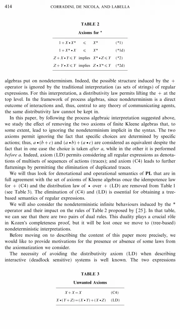
TABLE 2

Axioms for *

1+X vX* � X* (*1)

1+X* vX � X* (*1d)

Z+X vY�Y implies X* vZ�Y (*2)

Z+Y vX�Y implies Z vX*�Y (*2d)

algebras put on nondeterminism. Indeed, the possible structure induced by the +operator is ignored by the traditional interpretation (as sets of strings) of regularexpressions. For this interpretation, a distributivity law permits lifting the + at thetop level. In the framework of process algebras, since nondeterminism is a directoutcome of interactions and, thus, central to any theory of communicating agents,the same distributivity law cannot be kept in.

In this paper, by following the process algebraic interpretation suggested above,we study the effect of removing the two axioms of finite Kleene algebras that, tosome extent, lead to ignoring the nondeterminism implicit in the syntax. The twoaxioms permit ignoring the fact that specific choices are determined by specificactions; thus, a v (b+c) and (a vb)+(a vc) are considered as equivalent despite thefact that in one case the choice is taken after a, while in the other it is performedbefore a. Indeed, axiom (LD) permits considering all regular expressions as denota-tions of multisets of sequences of actions (traces); and axiom (C4) leads to furtherflattenings by permitting the elimination of duplicated traces.

We will thus look for denotational and operational semantics of PL that are infull agreement with the set of axioms of Kleene algebras once the idempotence lawfor + (C4) and the distribution law of v over + (LD) are removed from Table 1(see Table 3). The elimination of (C4) and (LD) is essential for obtaining a tree-based semantics of regular expressions.

We will also consider the nondeterministic infinite behaviours induced by the *operator and their impact on the rules of Table 2 proposed by [25]. In that table,we can see that there are two pairs of dual rules. This duality plays a crucial rolein Kozen's completeness proof, but it will be lost once we move to (tree-based)nondeterministic interpretations.

Before moving on to describing the content of this paper more precisely, wewould like to provide motivations for the presence or absence of some laws fromthe axiomatization we consider.

The necessity of avoiding the distributivity axiom (LD) when describinginteractive (deadlock sensitive) systems is well known. The two expressions

TABLE 3

Unwanted Axioms

X+X=X (C4)

X v(Y+Z)=(X vY)+(X vZ) (LD)

414 CORRADINI, DE NICOLA, AND LABELLA

TABLE 4

Basic Preorder

X�X+Y (PR)

X�Y and X$�Y$ imply X vX$�Y vY$ (R1)

X�Y and X$�Y$ imply X+X$�Y+Y$ (R2)

a v (b+c)=a vb+a vc are clearly language equivalent, as they both describe theset of strings [ab, ac]. However, when viewed as processes they have to be dis-tinguished. While the left-hand side can always perform an action b after action a,the right-hand side has the possibility of refusing to do so. Thus, if we assume thatthese two processes can interact with their environment, it is essential to considerthem as semantically different.

Axiom X+X=X, instead, is present in all process algebras axiomatizations.Nevertheless, if one wants to preserve the richness of the syntactic structure and, atthe same time, be faithful to tree models, then he may want to leave (C4) out. Anindependent, more semantic, motivation for eliminating the axiom stating idem-potence of + is the interest in formalizing fault-tolerant systems. As a simpleexample consider process a a+a corresponding to the nondeterministic composi-tion of two processes that can perform an a action and then successfully terminate.If a hardware fault leads to shutting down one of the processes (say a printer) ofa+a then it would still offer the expected behaviour (a printout would be obtainedfrom the alternative printer). The same cannot be said for process a; in fact, a faultof the system where a is located would be noticed (no printout would be obtained).Then, one would say that a+a is more tolerant to faults than a, in the sense thatit takes advantage of the different instances of the available resources.3

Another axiom, worthy of note, is X v0=0 that reduces to 0 all those agents thateventually reach a deadlocked state. This law is not present in the axiomatizationsof process algebras (an exception is [5]), but it is commonly used in formallanguages and automata theory, where a word is `àccepted'' by an automaton onlyif it allows a transition from the initial state of the automaton to a final one. Thismeans that, if a deadlocked state occurs before reaching the final state, the wholecomputation is ignored. If one wants to take into account the sequence of actionsperformed before reaching a deadlocked state, then he can take advantage of thepossibility of writing, at specification time, P v(1+Q) instead of P vQ. This wouldpermit `àccepting'' also the sequences of actions performed by P.

The rest of the paper is organized as follows. In Section 2, we will study a denota-tional semantics for finite (*-free) regular expressions. We will see that the freemodel of the new set of axioms is equivalent to a class of trees labelled over A.Trees are seen as sets of labelled runs (sets of traces) plus some information about


3 This kind of fault tolerance is known in the literature as ``cold redundancy'': different inactive copiesof the same process are maintained, and no form of restart is assumed; as soon as an alternative ischosen the others are immediately discarded.

TABLE 5

|-Induction Rule

Let X0=1Xn+1=1+X vXn

\n # N Xn vZ�Y implies X* vZ�Y (|-R)

the branching structure of the runs. This permits us to naturally transfer tech-niques and results developed for formal languages and regular sets to models ofnondeterminism.

In Section 3 we will introduce an operational semantics for finite (*-free) regularexpressions; it is based on a class of labelled transition systems detailed enough todescribe the number of equal actions a system may perform when in a given state.On the top of this operational semantics, we will introduce a preorder relation thatwe call resource simulation (r-simulation) and an equivalence relation that we callresource bisimulation (r-bisimulation). This equivalence will allow us to identify alland only those regular expressions that denote isomorphic trees. An importantproperty of the equivalence and the preorder (that will permit us to restrict atten-tion to the latter) is that r-bisimulation can be obtained as the kernel of r-simula-tion. We study in full detail the preorder Ir induced by r-simulation; we shallprove that the set of axioms obtained from Table 1 by removing (C4) and (LD)and adding the laws of Table 4 is consistent and complete with respect to Ir . Ofcourse, in Table 1, any equation T1=T2 should be read as T1�T2 and T2�T1 .

The complete axiomatization of r-bisimulation equivalence is obtained by remov-ing X�X+Y from that of the preorder.

In Section 4 we study the relationships between operational and denotationalsemantics and prove their coincidence.

Section 5 is dedicated to studying the impact of enriching the language with the*-operator and, thus, to considering the induced infinite behaviours. To avoid con-sidering infinite sequences of 1-actions (essentially internal chattering), we restrictattention to terms without iterations of 1's; i.e. we exclude terms with 1 or * sum-mands in a *-context. This essentially amounts to saying that we permit insertingin [�]*-context only those terms that do not have the empty word property, asdefined by Salomaa [30].

As we have already mentioned, not all theorems of [25] are sound for our inter-pretation. We have that axiom (*1d) does not hold,4 and that inference rule (*2d)of Table 2 is vacuously true; its premise holds only if Z=0 and X=1.5 For estab-


4 Processes 1+a* va and a* are trace equivalent but they are not equivalent for our interpretationbecause the term on the l.h.s. can execute two initial a-actions while that on the r.h.s can execute onlyone.

5 It could be of interest to know that, results in [10] (based on [Kro91]) imply that Kozen'saxiomatization is complete for the equational theory of regular sets also when laws (*1d) and (*2d) areremoved from the proof system.

File: 571J 163606 . By:SD . Date:19:11:99 . Time:08:17 LOP8M. V8.B. Page 01:01Codes: 2823 Signs: 2136 . Length: 52 pic 10 pts, 222 mm

lishing our completeness result, we replace (*2) with a more powerful |-inductionrule (see Table 5). The problem of establishing whether this is necessary is stillopen.

We rely on the correspondence between approximants of terms and those termsthat are built by unfolding via the rewriting rule

P* � 1+P vP*.

For the denotational semantics, these approximants allow us to build the inter-pretation of P* as a colimit and to obtain a complete proof system for the enrichedlanguage.

In the final section, we discuss extensions of the language with a binary operatorfor parallel composition and a complete axiomatization also for this richer languageand discuss further work on logical characterization and a weak version of resourcebisimulation.

2. FINITE DENOTATIONAL MODELS

In this section we provide a denotational semantics of finite (*-free) PL by inter-preting it over a category of labelled trees and show that it coincides with the initialmodel induced by a simple set of equations. For the full understanding of this sec-tion a basic knowledge of a few notions of category theory is required. To this pur-pose the reader is referred to an introductory book; see, e.g., [29] and referencestherein.

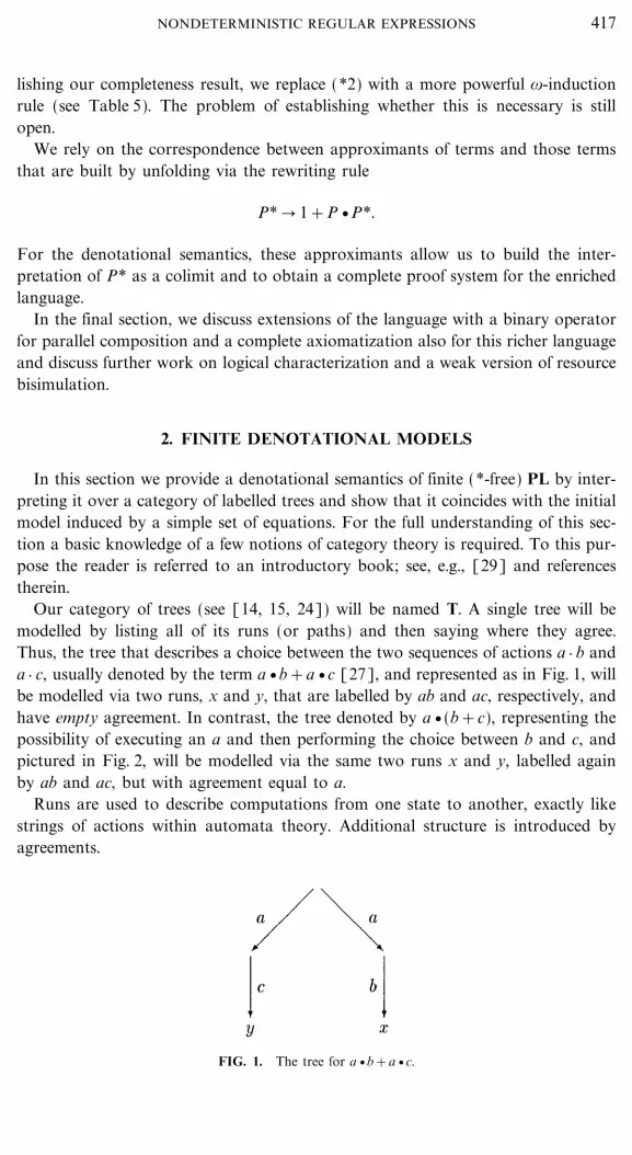
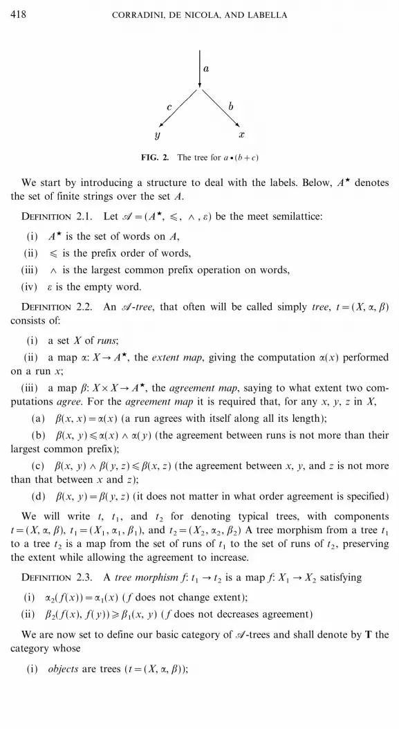
Our category of trees (see [14, 15, 24]) will be named T. A single tree will bemodelled by listing all of its runs (or paths) and then saying where they agree.Thus, the tree that describes a choice between the two sequences of actions a } b anda } c, usually denoted by the term a vb+a vc [27], and represented as in Fig. 1, willbe modelled via two runs, x and y, that are labelled by ab and ac, respectively, andhave empty agreement. In contrast, the tree denoted by a v(b+c), representing thepossibility of executing an a and then performing the choice between b and c, andpictured in Fig. 2, will be modelled via the same two runs x and y, labelled againby ab and ac, but with agreement equal to a.

Runs are used to describe computations from one state to another, exactly likestrings of actions within automata theory. Additional structure is introduced byagreements.

FIG. 1. The tree for a vb+a vc.


File: 571J 163607 . By:SD . Date:19:11:99 . Time:08:17 LOP8M. V8.B. Page 01:01Codes: 2713 Signs: 1640 . Length: 52 pic 10 pts, 222 mm

FIG. 2. The tree for a v (b+c)

We start by introducing a structure to deal with the labels. Below, AC denotesthe set of finite strings over the set A.

Definition 2.1. Let A=(AC, �, 7 , =) be the meet semilattice:

(i) AC is the set of words on A,

(ii) � is the prefix order of words,

(iii) 7 is the largest common prefix operation on words,

(iv) = is the empty word.

Definition 2.2. An A-tree, that often will be called simply tree, t=(X, :, ;)consists of:

(i) a set X of runs;

(ii) a map :: X � AC, the extent map, giving the computation :(x) performedon a run x;

(iii) a map ;: X_X � AC, the agreement map, saying to what extent two com-putations agree. For the agreement map it is required that, for any x, y, z in X,

(a) ;(x, x)=:(x) (a run agrees with itself along all its length);

(b) ;(x, y)�:(x) 7 :( y) (the agreement between runs is not more than theirlargest common prefix);

(c) ;(x, y) 7;( y, z)�;(x, z) (the agreement between x, y, and z is not morethan that between x and z);

(d) ;(x, y)=;( y, z) (it does not matter in what order agreement is specified)

We will write t, t1 , and t2 for denoting typical trees, with componentst=(X, :, ;), t1=(X1 , :1 , ;1), and t2=(X2 , :2 , ;2) A tree morphism from a tree t1

to a tree t2 is a map from the set of runs of t1 to the set of runs of t2 , preservingthe extent while allowing the agreement to increase.

Definition 2.3. A tree morphism f: t1 � t2 is a map f: X1 � X2 satisfying

(i) :2( f (x))=:1(x) ( f does not change extent);

(ii) ;2( f (x), f ( y))�;1(x, y) ( f does not decreases agreement)

We are now set to define our basic category of A-trees and shall denote by T thecategory whose

(i) objects are trees (t=(X, :, ;));


(ii) arrows are tree morphisms;

(iii) identities (idt=idX) are defined in terms of identities over set of runs;

(iv) composition (g b f ), is given by function composition.

With Tfin we will denote the subcategory of finite trees.

Definition 2.4. A tree morphism is a strict (or regular) monomorphism if f isinjective and ;2( f (x), f ( y))=;1(x, y)

Note that in Tfin if f1 : t1 � t2 and f2 : t2 � t1 are strict monomorphism then t1

and t2 are isomorphic. Indeed, we have that a strict monomorphism is an injectivetree morphism such that both extent and agreement are preserved. It might be ofinterest to know that, in categorical terms, strict monomorphisms are regularmonomorphisms, i.e. equalizers.

Proposition 2.5. T has an initial object, given by the empty tree 0=(<, <, <),and it has coproducts � .

Proof. There is clearly a unique map from 0 to any tree t, namely the emptymap 0t . For two trees t1 and t2 , t1 � t2 is defined as (X1 _+ X2 , :1 _+ :2 , ;1 _+ ;2),(where _+ denote disjoint set union and ;1 _+ ;2 denotes the agreement function thatbehaves as ;1 on pairs from X1 , as ;2 on pairs from X2 , and is = on mixed pairs)Clearly, the canonical injections

v i1 : t1 � t1 � t2

v i2 : t2 � t1 � t2

are strict monomorphisms. K

In the next definition we introduce a concatenation operator between trees andthen we prove that it is a tensor product, i.e. an associative binary functor withunity.

Definition 2.6. Given two trees, t1=(X1 , :1 , ;1) and t2=(X2 , :2 , ;2) sequen-tial composition � is defined as follows (here } is used to denote string concatena-tion): t1 � t2=(X, :, ;) , where

�� X=X1_X2 (a run in t is a run of t1 followed by a run of t2);

�� :((x1 , x2) )=:1(x1) } :2(x2) (the labels of runs in t are obtained by con-catenating those of the arguments);

�� ;((x1 , x2) , ( y1 , y2) )

=;1(x1 , y1) } ;2(x2 , y2),=;1(x1 , y1),

if x1= y1 ,otherwise

(the agreement between the second components of two composite runs is con-sidered only if the runs have a common initial part).

Proposition 2.7. Sequential composition � is a tensor product with object unittree 1=( v , :( v )==, ;( v , v )==) and T is monoidal w.r.t. � .


TABLE 6

Axioms for Finite NondeterministicRegular Expressions

X+Y=Y+X (C1)(X+Y)+Z=X+(Y+Z) (C2)

X+0=X (C3)

(X vY) vZ=X v(Y vZ) (S1)X v1=X (S2)1 vX=X (S3)X v0=0 (S4)0 vX=0 (S5)

(X+Y) vZ=(X vZ)+(Y vZ) (RD)

Terms of PL can be interpreted as trees in the category T by means of a functionT defined by induction on the structure of terms.

Definition 2.8 (Denotational semantics). An algebraic interpretation of finitePL terms is obtained by associating to them a tree in T via function T:

�� T�0�=0,

�� T�1�=1,

�� T�a�=(x, :(x)=a, ;(x, x)=a),

�� T�P+Q�=T�P� �T�Q�,

�� T�P vQ�=T�P� �T�Q�.

If we restrict ourselves to the subcategory Tfin of finite trees, we can prove thatTreefin, the set of its objects, is the free model for the axioms of Table 6, i.e. thoseof Table 1 without those of Table 3.

For proving the main theorem of this section, we need a lemma that allows usto reduce PL-terms to standard forms.

Definition 2.9 (Normal forms). A normal form is either 0 or a term of theform

\:i # I

a i+ :j # J

a j vn j++ :k # K

Pk ,

where Pk=1 for all k and for all j we have that nj is a normal form different from0 and 1.

Lemma 2.10 (Reduction to normal forms). Every finite PL term P is provablyequal, via the laws of Table 6, to a normal form nf (P).

Proof. The proof proceeds by induction on the depth of terms, defined by

depth(0)=0

depth(1)=depth(a)=1

depth(P+Q)=max[depth(P), depth(Q)]

depth(P vQ)=depth(P)+depth(Q).


Let us assume that the claim holds for terms P with depth(P)<n. We prove itfor terms P of depth n. The proof proceeds by (inner) induction on the syntacticstructure of terms.

(1) In case P=0, P=a and P=1 the claim follows trivially: nf (P)=P.

(2) P=P1+P2 . By structural induction there exist two normal forms nf (P1)and nf (P2) such that P1=nf (P1) and P2=nf (P2). To obtain nf (P1+P2), we per-form a case analysis:

(a) nf (P1)=0 and nf (P2){0. Then P1+P2=nf (P1)+nf (P2)=0+nf (P2)=nf (P2) by axiom (C3) and nf (P2) is a normal form.

(b) nf (P1){0 and nf (P2)=0. Then P1+P2=nf (P1)+nf (P2)=nf (P1)+0=nf (P1) by axiom (C3) and nf (P1) is a normal form.

(c) nf (P1)=0 and nf (P2)=0. Then P1+P2=nf (P1)+nf (P2)=0+0=0 byaxiom (C3) and 0 is a normal form.

(d) nf (P1){0 and nf (P2){0. Then P1+P2=nf (P1)+nf (P2) is a normalform by axioms (C1) and (C2).

(3) P=P1 vP2 . By structural induction there are two normal forms nf (P1) andnf (P2) such that P1=nf (P1) and P2=nf (P2). We distinguish now a few cases toobtain a normal form nf (P1 vP2):

(a) nf (P1)=0 and nf (P2){0. Then P1 vP2=nf (P1) vnf (P2)=0 vnf (P2)=0by axiom (S5) and hence nf (P1 vP2)=0.

(b) nf (P1){0 and nf (P2)=0. Symmetric of a, use (S4) instead of (S5).

(c) nf (P1)=0 and nf (P2)=0. Then P1 vP2=nf (P1) vnf (P2)=0 v0=0 byaxiom (S4) and, hence, nf (P1 vP2)=0.

(d) nf (P1)=1 and nf (P2){1. Then P1 vP2=nf (P1) vnf (P2)=1 vnf (P2)=nf (P2) by axiom (S3) and nf (P1 vP2)=nf (P2).

(e) nf (P1){1 and nf (P2)=1. Symmetric of d, use (S2) instead of (S3).

(f) nf (P1)=1 and nf (P2)=1. Then P1 vP2=nf (P1) vnf (P2)=1 v1=1 byaxiom (S2) and hence, nf (P1 vP2)=1.

(g) nf (P1){0, 1 and nf (P2){0, 1. Then

P1 vP2

=nf (P1) vnf (P2)

=\\:i # I

a i+ :j # J

aj vnj ++ :k # K

Pk[Pk=1]+ vnf (P2)

by axiom (RD),

=\\:i # I

a i+ vnf (P2)+\ :j # J

aj vnj + vnf (P2)++\ :k # K

Pk[Pk=1]+ vnf (P2)

by axiom (RD),


=\:i # I

ai vnf (P2)+ :j # J

(aj vnj) vnf (P2)++ :k # K

Pk[Pk=1] vnf (P2)

by axioms (S1), (S3),

=\:i # I

ai vnf (P2)+ :j # J

aj v(nj vnf (P2))++ :k # K

nf (P2)

by inductive hypothesis (depth(nj vnf (P2))<n),

=\:i # I

ai vnf (P2)+ :j # J

aj vnf (nj vnf (P2))++ :k # K

nf (P2)

Now, to prove the claim, it suffices to notice that the final term is a sum of nor-mal forms and can thus be reduced to a normal form (see item 2 above). K

Theorem 2.11 (Treefin is the free model of (*-free) nondeterministic regularexpressions.) (Treefin, � , � , 0, 1) is equivalent to the free model induced by thelaws of Table 6.

Proof. Given a term in the language PL, we can associate with it a unique (upto isomorphism) tree. To show that every tree has a unique description in the termalgebra quotiented by our laws, we describe the normal form corresponding to eachtree and prove that two different normal forms give rise to nonisomorphic trees.

We start by showing that any tree can be seen as a normal form; i.e., given a treet=(X, :, ;), there exists a normal form n such that T�n�=t.

The simplest case is when t=(X, :, ;) with X=<. Then t coincides with T�0�.If X{< we proceed by induction on d(t), the depth of t, defined here as the

length of run x # X with maximum extent.Assume d(t)=0. In this case \x # X, :(x)== and T��k # [1 } } } |X| ] Pk[Pk=1]�

=t. Assume now d(t)>0. For every a # A, consider set Xa=[X 1a , ..., X k

a], whereX j

a=[xi | ;(xj , x i)=a]. Intuitively, set X ja contains all runs x i # X that have agree-

ment greater or equal than a. Clearly, X ja=X i

a for every x i # X ja . Every X j

a # Xa

induces a tree t ja=(X j

a , : ja , ; j

a), where : ja and ; j

a are the obvious restrictions of :and ; over set of runs X j

a . We will show that for every X ja # Xa there exists a nor-

mal form n ja such that T�n j

a �=t ja so that na=� j # [1 } } } k] n j

a is a normal form fortree ta=(X 1

a _ } } } _ X ka , :a , ;a) with :a and ;a the restrictions of : and ; over set

of runs X 1a _ } } } _ X k

a . Since there is a finite number of a # A such that Xa {<,it follows that t=T��a # A, Xa{< na �. Thus, take X j

a # Xa and consider treet j

a=(X ja , : j

a , ; ja).

If d(t)=1 then \x # X ja , :(x)=a and we have either t j

a=T�a� if |X ja |=1 or

t ja=T�a v�k # |X j

a| Pk[Pk=1]� if |X ja |>1.

Assume now, by induction hypothesis, that for every t ja such that 1<d(t j

a)�nthere exists a normal form n j

a such that T�n ja �=t j

a . We prove that the statementfor any t j

a with d(t ja)=n+1. In this case X j

a induces a tree ta$j=(X j

a , :a$j , ;a$

j), where:a$

j and ;a$j are defined by :a$

j(x ja)=w if :(x j

a)=aw and ;a$j(x i

a , x ja)=w if

;(x ia , x j

a , )=aw for x ia , x j

a # X ja . Clearly, d(t j

a)>d(ta$j); thus by induction hypothesis

there exists a normal form n$ ja such that T�n$ j

a �=t$ ja and, hence, T�a vn$ j

a �=t ja .


It remains to be proven that two different normal forms give rise to non-isomorphic trees. But this immediately follows by an inspection of the normalforms. Indeed if they differ over summands Pk with Pk=1 then they have a dif-ferent number of 1-summands and, hence, the corresponding trees cannot beisomorphic. Similarly, if they differ over summands a. For summands of the forma vn the claim follows from an inductive reasoning. K

3. OPERATIONAL AND OBSERVATIONAL MODELS

Here we provide an observational account of finite nondeterministic regularexpressions, by interpreting them as equivalence classes of labelled transitionsystems. The proposed equivalence relies on the same recursive pattern of bisimula-tion but takes into account also the number of equivalent states that are reachablefrom a given one.

Definition 3.1. A labelled transition system is a triple (Z, L, T) , where

�� Z is a set of states,

�� L is a set of labels

�� T is a transition relation; T�Z_L_Z.

The elements of T will often represented as q w�l q$, rather than as triples; thus,we shall write z w�l z$, instead of (z, l, z$) # T.

In our case, states are terms of PL (as defined in the Introduction) and labels arepairs (+, u) with + # A _ [1] and u a term, called choice sequence, generated by

u ::== | lu | ru with l, r tags.

The transition relation relies on the predicate defined in Table 7 and is definedin Table 8. For those familiar with the operational semantic of process algebras, wewould like to remark that 1-actions do not play the same role of invisible {-actions.They simply stand for successfully terminated states.

We have two kinds of transitions:

v P ww�(a, u) P$: P performs an action a, possibly preceded by 1-actions withchoice sequence u.

v P ww�(1, u) 1: P performs 1-actions to reach process 1 with choice sequence u.

TABLE 7

Active Predicate

active(1)

active(a)

active(P) 6 active(Q) O active(P+Q)

active(P) 7 active(Q) O active(P vQ)


TABLE 8

Operational Semantics for PL

(Tic)1 ww�

(1, =)1

(Atom)a ww�

(a, =)1

(Sum1)P ww�

(+, u) P$

P+Q ww�(+, lu) P$

(Sum2)Q ww�

(+, u) Q$

P+Q ww�(+, ru) Q$

(Seq1)P ww�

(a, u) P$, active(Q)

P vQ ww�(a, u) P$ vQ

(Seq2)P ww�

(1, u)1, Q ww�

(+, u$) Q$

P vQ ww�(+, uu$) Q$

These transitions are atomic; they cannot be interrupted and they keep no trackof intermediate states. In both cases, u is used to keep information about thepossible nondeterministic structure of P and will permit distinguishing those trans-itions of P whose action label and target state have the same name. Thus for a+a,it is possible to record that it can perform two different a actions: a+a ww�(a, l) 1and a+a ww�(a, r) 1. Without l and r, we would have only the a+a w�a 1 transition.

The predicate active over PL processes used in Seq1 allows us to detect emptyprocesses and to avoid performing actions leading to deadlock.

The rules of Table 8 should be self-explanatory. We only comment on those for+ and v .

The rule for P+Q says that if P can perform (+, u) to become P$ then P+Qcan perform (+, lu) to become P$, where l records that action + has been perfor-med by the left alternative. The right alternative is dealt with symmetrically. (Seq1)mimics sequential composition of P and Q; it states that if P can perform (+, r)then P vQ can evolve with the same label to P$ vQ. The premise active(Q) of theinference rule ensures that Q can successfully terminate. Note that active(Q) in(Seq1) could be replaced by _Q$ } Q ww�(+, u$) Q$, that is by requiring Q to performany transition. This choice, however, would require a ``look ahead'' that would beheavy when mechanically checking successful termination of a process. We can,instead, statically check whether a process eventually reaches a deadlock state.

In order to abstract from choice sequences while keeping information about thealternatives a process has for performing a specific action, we introduce a newtransition relation that associates to every pair (P # PL, + # Act _ [1]) , a multisetM, representing all processes that are target of (+, u)-transitions from P. It isdefined as the least relation such that

P w�+ [|P$ | _u } P ww�(+, u)

P$|].

Thus, we have

v a+a w�a [|1, 1|] because

�� a+a ww�(a, l) 1

�� a+a ww�(a, r) 1;


v (1+1) v(a+a) w�a [|1, 1, 1, 1, |] because

�� (1+1) v(a+a) ww�(a, ll) 1

�� (1+1) v(a+a) ww�(a, lr) 1

�� (1+1) v(a+a) ww�(a, rl) 1

�� (1+1) v(a+a) ww�(a, rr) 1.

We also have that 1+1 w�1 [|1, 1|] while 1 w�1 [|1|]. Here we would like toremark that, with the proposed semantics, we can count also 1-transitions. If we didnot have this possibility, we would have been forced to identify X+X and X by(1+1) vX and 1 vX.

3.1. Resource Simulation and Resource Bisimulation

Very often descriptions via labelled transition systems turn out to be too con-crete. To abstract from `ìrrelevant'' details and for relating different descriptions ofthe same system, the notions of behavioral relations (equivalences or preorders) areoften used. Different opinions about the relevant features of concurrent systems tobe taken into account and, thus, about the aspects that can be ignored have led toa number of behavioral relations. A few of these notions are based on the notionsof bisimulation. Intuitively, two systems are bisimulation equivalent whenever theycan perform the same sequences of actions to reach (via them) bisimulation equiv-alent states.

In this subsection, we will introduce two new bimulation-based relations that aimat identifying only those systems that have exactly the same behaviour and, thus,differ only for their syntactic structure. We will introduce an equivalence relation,resource bisimulation, that relates only those terms whose unfolding, via the opera-tional semantics, gives rise to isomorphic labelled trees. We will also introducea preorder, resource simulation, that ``captures'' the notion of tree embedding.A preliminary report on the result of this section appeared as [13].

The transition relation w�+ , introduced above, is the basis for defining resourcesimulation and resource bisimulation.

Definition 3.2 (Resource simulation and resource bisimulation). 1a. A rela-tion R�PL_PL is a r-simulation if for each (P, Q) # R and for each + # A _ [1]:P w�+ M implies Q w�+ M$ and _f injective: M � M$, s.t. \P$ # M, (P$, f (P$)) # R;

1b. P and Q are r-similar (P Ir Q) if there exists a r-simulation R containing(P, Q) .

2a. A relation R�PL_PL is a r-bisimulation if for each (P, Q) # R, and foreach + # A _ [1]:

�� P w�+ M implies Q w�+ M$ and _f injective: M � M$, s.t. \P$ # M,(P$, f (P$)) # R;

�� Q w�+ M$ implies P w�+ M and _g injective: M$ � M, s.t. \Q$ # M$,(Q$, g(Q$)) # R;

2b. P and Q are r-bisimilar (Ptr Q), if there exists a r-bisimulation R contain-ing (P, Q).


The above definitions should be self-explanatory. We want simply to remark thatthe injection f: M � M$ is used to ensure that different (indexed) processes in M aresimulated by different (indexed) processes in M$.6 Thus r-bisimilarity requires thecardinality of M be less or equal to the cardinality of M$.

With standard techniques it is possible to show that tr is an equivalence relationand it is preserved by nondeterministic composition and sequential composition. Itis not difficult to check that a Ir a+a, at% r a+a, a+btr b+a, and(1+1) vatr a+a.

The following propositions provide soundness and completeness results for theaxiomatization of r-simulation and r-bisimulation over finite PL terms.

First, we will prove that the laws of Table 6, an inequational rule, X�X+Y,that captures the essence of resource simulation, and two inference rules statingmonotonicity of � with respect v and + (see Table 4) soundly and completelyaxiomatize r-simulation over finite PL. Clearly, X=Y in Table 6 has to be intendednow as X�Y and Y�X.

Then, we will prove that the laws of Table 1, without of those in Table 3, are suf-ficient to axiomatize r-bisimulation over finite PL.

First we establish a congruence result for our preorder.

Proposition 3.3. Resource simulation is preserved by all PL operators.

Proof. We just prove the statement for v which is the most involved case. Theproof for + is simpler. We prove that given X Ir Y and R Ir S; we haveX vR Ir Y vS. To prove this result, we show that

R=[(X vR, Y vS) | X Ir Y and R Ir S] _ R1 _ R2 ,

where R1 and R2 are the simulation relations used to establish X Ir Y and R Ir S,is a resource simulation. Assume (X vR, Y vS) # R and X Ir Y, R Ir S. ConsiderX vR w�+ M. Then we prove that Y vS w�+ M$ and _f injective: M � M$, s.t.\P # M, (P, f (P)) # R. We distinguish two cases depending on +=1 or +=a:

�� +=1. Then M=[|P | P=1|]. If |M|=k, then there are k transitions of theform X vR ww�(1, ui) 1 for i # [1 } } } k]. By an inspection of the rules in Table 8 thesetransitions are of the form X ww�(1, u$) 1 and R ww�(1, u"i) 1 with ui=u$iui" . Now, sinceX Ir Y, for every X ww�(1, u$i) 1 there exists a different Y ww�(1, v$i) 1 and, since R Ir S,for every R ww�(1, u"i) 1, there exists a different S ww�(1, v"i) 1. Thus, for every X vRww�(1, u$i u"i ) 1 there exists a different Y vS ww�(1, v$iv"i) 1 in M$. It follows that there exists aninjection from M to M$.

�� +=a and consider X vR w�+ M. Note that every process in M can be eitherof the form X$ vR or of the form R$. In particular, the former processes are targetof transitions X vR ww�(a, u) X$ vR if X ww�(a, u) X$, while the latter processes aretarget states of transitions of the form X vR ww�(a, u) R$ if X ww�(1, u$) 1, R ww�(a, u") R$and u=u$u". Clearly, since X Ir Y, every transition X vR ww�(a, u) X$ vR withX ww�(a, u) X$ has a different transition Y vS ww�(a, v) Y$ vS with Y ww�(a, v) Y$ and


6 Since a multiset can be seen as a set of indexed elements, an injection between multisets will be seenjust as an ordinary injection between sets.

(X$ vR, Y$ vS) # R. Similarly, since X Ir Y and R Ir S, every transition X vRww�(a, u) R$ with X ww�(1, u$) 1 and R ww�(a, u") R$ and u=u$u" has a different transitionY vS ww�(a, v) S$ with Y ww�(1, v$) 1, S ww�(a, v") S$, v=v$v", and (R$, S$) # R2 . K

Proposition 3.4 (Completeness for r-simulation). The laws of Table 6 andTable 4 soundly and completely axiomatize r-simulation over finite PL.

Proof. It is possible to show that the following statements hold, once we let �denote the preorder over finite PL terms induced by the rules of Table 4:

Soundness. For all finite PL terms P and Q, P�Q implies P Ir Q. This can beproved by showing the appropriate resource simulations. Here we just prove sound-ness of axioms (S2) and (RD). All the other axioms can be proven similarly.

To show that X v1=X, we prove that both X v1 Ir X and X Ir X v1 hold.These two statements follow the fact that relations

R=[(X v1, X) | X # PL] _ [(1, 1)]; R$=[(X, X v1) | X # PL] _ [(1, 1)]

are resource simulations. Indeed,

(1) X v1 ww�(1, +) 1 iff X ww�(1, +) 1

(2) X v1 ww�(a, u) iff X ww�(a, u) X$

can be easily proven by a simple inspection of the operational rules.To prove that (X+Y) vZ=(X vZ)+(Y vZ), we prove that (X+Y) vZ Ir

(X vZ)+(Y vZ) and that (X vZ)+(Y vZ) Ir (X+Y) vZ. Again this follows byshowing that relations

R=[((X+Y) vZ, (X vZ)+(Y vZ)) | X, Y, Z # PL] _ id;

R$=[((X vZ)+(Y vZ), (X+Y) vZ) | X, Y, Z # PL] _ id

are resource simulations. This can be proven via the items that are direct conse-quences of the operational semantics:

(1) (X+Y) vZ ww�(+, lu) R iff (X vZ)+(Y vZ) ww�(+, lu) R;

(2) (X+Y) vZ ww�(+, ru) R iff (X vZ)+(Y vZ) ww�(+, ru) R.

Completeness. For all normal forms n1 and n2 , n1 Ir n2 implies n1�n2 . Thisresult can be proven as in [27] by using axioms in Table 6. The proof proceeds byinduction on depth(n1)+depth(n2). Assume the statement for depth(n1)+depth(n2)<n and prove it for depth(n1)+depth(n2)=n. Let n1 and n2 be

n1 = :i # I

ai+ :j # J

aj vn j+ :k # K

[Pk=1];

n2= :l # L

bl+ :m # M

bm vsm+ :n # N

[Pn=1].

Moreover, by hypothesis we have n1 Ir n2 . Let [a1 , a2 , ..., an] be the set of initialactions appearing in n1 ; that is, [a1 , a2 , ..., an]=[ai | i # I] _ [aj | j # J]. Then forproper subsets of I, J, L, and M,


n1 =\ :1i # I1

[a1i=a1]+ :1j # J1

a1 vn1j++ } } } +\ :ni # In

[ani=an]+ :nj # Jn

an vnnj++ :

k # K

[Pk=1];

n2=\ :1l # L1

[b1l=a1]+ :1m # M1

a1 vs1m++ } } } +\ :nl # Ln

[bni=an]+ :nm # Ln

an vsnm++ :

n # N

[Pn=1]+r,

where r is a normal form that does not have initial [a1 , a2 , ..., an]-actions andinitial 1-actions. By the definition of resource simulation, it is easy to see that

(i) for every o # [1 } } } n],

\ :oi # Io

[aoi=ao]+ :oj # Jo

ao vnoj+ Ir \ :ol # Lo

[bol=ao]+ :om # Mo

ao vsom +(ii) and summations of 1's are related:

:k # K

[Pk=1] Ir :n # N

[Pn=1].

Thus, if we are able to prove the main result for (i) and (ii), then by axioms (R2)and (PR) (useful to deal with r in n2) we are also able to prove that n1�n2 . Wejust prove (i) because (ii) is clearly simple. Again we prove (i) when o=1; all othercases follow similarly. Assume

\ :1i # I1

[a1i=a1]+ :1j # J1

a1 vn1j+ Ir \ :1l # L1

[b1l=a1]+ :1m # M1

a1 vs1m + . (1)

Then

:1i # I1

[a1i=a1]+ :1j # J1

a1 vn1j w�a1

[| 1, ..., 1|I1 | times

, n1j1, ..., n1j|J1|

|]=M,

where every n1jiis different from 1 by definition of the normal form. Similarly,

:1l # L1

[b1l=a1]+ :1m # M1

a1 vs1m w�a1

[| 1, ..., 1|L1 | times

, s1m1, ..., s1m|M1|

|]=M$.

By hypothesis there exists an injection f: M � M$ such that \P # M, P Ir f (P).We have to distinguish three cases:

(a) P=1 and f (P)=1. Then we have 1�1 by axiom (R1) is a1 v1�a1 v1.Finally, by axiom (S2) is a1�a1 .


(b) P=1 and f (P)=s1mkfor some k. Then necessarily s1mk

has a summand 1and, hence, by axiom (PR) (and (C1), (C2)) it follows that 1�s1mk

. Thus, also,a1 v1�a1 vs1mk

and by axiom (S2) is a1�a1 vs1mk.

(c) P=n1jkfor some k. Then f (P) cannot be 1. Let f (P)=s1mk$

for some k$. Herewe can apply induction hypothesis to prove that n1jk

�s1mk$. By axiom R1, a1 v

n1jk�a1 vs1mk$

.

Items (a), (b), and (c) above show that every summand of �1i # I1[a1i=a1]+

�1j # J1a1 vn1j is provably � to a summand of �1l # L1

[b1l=a1]+�1m # M1a1 vs1m .

Thus, in order to complete the proof for (1) we just need to eventually apply axiom(PR) (note, indeed, that the latter summation may have more summands of theformer one). K

Similarly, we can establish the corresponding result for r-bisimulation.

Proposition 3.5 (Completeness for r-bisimulation). The laws of Table 6 soundlyand completely axiomatize r-bisimulation over finite PL.

3.2. A Preorder Whose Kernel is Resource Equivalence

In this section we show that the kernel of Ir coincides with resource equiv-alence. This result is new for simulation-like semantics; for example, it does nothold for the classical simulation preorder of [27, 28]. In that case we have thatbisimulation cannot be obtained as a double simulation.7 The usefulness of thiscoincidence result is twofold. First of all, it permits concentrating just on the preor-der and to obtain as corollary many results (like the last theorem of the previoussection) for the equivalence. Second, it permits using this behavioral relation forstepwise refinements of systems implementation.

In order to establish this property, we show that the set of pairs (P, Q) of PLprocesses such that P Ir Q and Q Ir P is a resource bisimulation. This will be animmediate consequence of the following two lemmas. They permit us to concludethat, given two sets of PL processes, S and S$, and two injections f: S � S$,g: S$ � S such that \s # S, s Ir f (s) and \s$ # S$, s$ Ir g(s$), then for each s # S wehave s Ir f (s) and f (s) Ir s (s$ Ir g(s$) and g(s$) Ir s$), and similarly for s$.

Lemma 3.6. Let S=[P1 , ..., Pn] and S$=[Q1 , ..., Qn] be two sets of PL pro-cesses and f: S � S$, g: S$ � S be two injections such that \Pi # S, Pi Ir f (Pi) and\Qi # S$, Qi Ir g(Qi). Then for each Pi1

# S, i1 # n[1 } } } n] there exists a chainPi1

Ir Q i1Ir Pi2

Ir Qi2Ir } } } Ir Qim

Ir Pi1for some m # [1 } } } n], [i1 , ..., im]�

[1 } } } n], Pij# S, Qij

# S$ and Pij{Pik

, Qij{Qik

for each j{k.

Proof. The existence of the chain follows by construction. Consider the chainPi1

Ir Q i1Ir } } } Ir Pij

Ir QijIr Pij+1

Ir } } } Ir QimIr Pi1

such that Q i= f (Pij)

and Pij+1= g(Q ij

) for each j # [1 } } } m&1]. Clearly, it is Pij# S and Qij

# S$. Provethat Pij

{Pikfor each j{k. Consider in the construction the first index m such that

there exists 2�l<m for which Pil=Pim

. But then, since g is an injection it isQil&1

=Qim&1, where g(Qil&1

)=Pijand g(Q im&1

)=P im, and since f is an injection it


7 Consider terms a vb and a+(a vb). According to Park and Milner's definitions, we have that a vbsimulates a+(a vb) and that a+(a vb) simulates { vb, but they are not bisimilar.

is Pil&1=Pim&1

, where f (Pil&1)=Qil&1

and f (Pim&1)=Qim&1

. But this is impossiblebecause m is the minimum index such that Pil

=Pim. Thus, all Pij

are different andfor symmetrical arguments all Qij

are also different.Finally we prove that the above chain ends with Pi1

. Suppose that QimIr Pi1

forno index m; that is, g(Qim

)=Pi1for no index m. Since card(S)=n and card(S$)=n

(where card(S) denotes the cardinality of finite set S) and every time we take a dif-ferent process from S and S$, we can assume that Pi1

Ir Q i1Ir } } } Ir Pin

Ir Qinand g(Qin

){Pi1. This is absurd. In fact g is an injection, thus g(Qin

) # S, but ifg(Qin

){Pi1then g(Qin

)=Pijfor some j{1. By construction, also, g(Qij&1

)=Pijand

Qij&1{Q in

because all Qijin the chain are different. Now since g is an injection and

it is not possible to have g(Qij&1)=g(Qin

)=Pijfor Qij&1

{Qin. Hence, Qin

=Pi1. It

follows that there exists an index m such that g(Qim)=Pi1

. K

Lemma 3.7. Let S=[P1 , ..., Pn] and S$=[Q1 , ..., Qn] be sets of PL processesand f: S � S$, g: S � S be two injections such that \Pi # S, Pi Ir f (Pi) and \Qi # S$,Qi Ir g(Q i). Then for each Pi # S, i # [1 } } } n], Pi Ir f (Pi) and f (Pi) Ir Pi (thereexists an injection r: S$ � S such that r( f (Pi))=Pi).

Proof. Let us suppose the existence of some Pi1, i1 # [1 } } } n], such that

Pi1Ir f (P i1

) but f (Pi1I% r Pi1

. By Lemma 3.6 there exists a chain starting by Pi1,

Pi1Ir Q i1

Ir Pi2Ir Qi2

Ir } } } Ir Q imIr Pi1

such that all Pijare different apart

from Pi1. Moreover, we know by hypothesis that Qi1

= f (Pi1) and g(Qi1

)=Pi2{Pi1

.Since Ir is a preorder it is transitive and then we have that Pi1

Ir Pi2Ir } } } Ir Pi1

and Qi1Ir Q i2

Ir } } } Ir Qim. Hence, also Q i1

Ir Qim. Since Qim

Ir Pi1follows by

transitive property Qi1Ir P i1

. This contradicts the hypothesis because Qi1is just

f (Pi1). K

The coincidence between the kernel of resource simulation and resource equiv-alence is established by the following proposition.

Proposition 3.8. For processes P and Q, Ptr Q iff P Ir Q and Q Ir P.

Proof. The case Ptr Q implies P Ir Q and Q Ir P follows by definitions of tr

and Ir . To prove it vice versa we show that

R=[(P1 , Q1) | P1 Ir Q1 and Q1 Ir P1]

is a r-bisimulation.Consider a generic pair (P1 , Q1) # R. Then it is P1 Ir Q1 and Q1 Ir P1 . It

follows that for each action + # A _ [1] we have

�� P1 w�+ M implies Q1 w�+ M$ and there exists an injection f: M � M$ such that\P$ # M is P$ Ir f (P$);

�� Q1 w�+ M$ implies P1 w�+ M and there exists an injection g: M$ � M such that\Q$ # M$ is Q$ Ir g(Q$).

To prove that R is a resource bisimulation we have to show that both(P$, f (P$)) # R and ( f (P$), P$) # R. By Lemma 3.7 we have that \P$ # M,P$ Ir f (P$) and f (P$) Ir P$. Thus, (P$, f (P$)) and ( f (P$), P$) are in R. Hence,R is a resource bisimulation and, since (P, Q) # R, it follows that Ptr Q. K


4. COMPARING OBSERVATIONAL AND DENOTATIONAL SEMANTICS

In this section we compare observational and denotational semantics of regularexpressions. To conclude that they coincide, it would be sufficient to observe thatthey are sound and complete with respect to the same set of axioms. We can,however, exhibit a more direct correspondence by showing that the tree obtainedby unfolding the transition system associated to P, LTS(P), is isomorphic to thetree obtained by interpreting process P via the interpretation function T.

Clearly, the direct correspondence between the two semantics offers us differenttechniques for establishing properties of our formalism. For example, Proposi-tion 4.2, Proposition 4.3, and Theorem 4.4 give an alternative way of provingProposition 3.8.

Definition 4.1. Let P be a term:

�� LTS(P) denotes the transition system associated to P according to the trans-ition rules in Table 8;

�� run(P) denotes the set of transition sequences, called runs or computationsP ww�(+1 , u1) P1 ww�(+2 , u2) } } } wwww�(+n&1, un&1) Pn&1 ww�(+n , un) 1 with P1 , ..., Pn&1 {1 performedby P;

�� forget is a function from runs to sequences of actions. Given a run x,P ww�(+1 , u1) P1 ww�(+2 , u2) } } } wwww�(+n&1 , un&1) Pn&1 ww�(+n , un) P$, forget(x)=+1 +2 } } } +n&1 +n

extracts the sequence of performed actions, where we let + be equal to = if +=1,or otherwise +=+.

�� We define the weight of a transition system as the sum of the weights of itsruns, that is, weight(LTS(P))=�i weight(xi), where xi # run(P). The weight of arun x is defined by weight(x)=0 if forget(x)== and weight(x)=n if forget(x)=a1 a2 } } } an&1an . We also let weight(P)=weight(LTS(P)).

�� The tree associated to LTS(P) is Unf(P)=(X, :, ;), defined by X=[x | x # run(P)], :(x)=forget(x), ;(x, y)=forget(x 7 y), where x 7 y denotes thelargest common prefix of x and y.

The following two propositions will be useful to prove that observational anddenotational semantics do coincide.

Proposition 4.2. Unf(P) and T�P� are isomorphic.

Proof. The proof proceeds by induction on the syntactic structure of P:

1. P=0. The transition system associated to process 0, LTS(0), is([0], <, <) and its unfolding is unf(0)=(<, <, <) that coincide with T�0�.

2. P=1. The transition system associated to process 1, LTS(1), is ([1],[(1, =)], [1 ww�(1, =) 1]) and its unfolding Unf(1)=([x], :(x)==, ;(x, x)==)with x=1 ww�(1, =) 1. The unfolding coincides with T�1�.

3. P=P1+P2 . Let LTS(P1)=(Z1 , L1 , T1) and LTS(P2)=(Z2 , L2 , T2) bethe transition systems associated to P1 and P2 , respectively. By inductionhypothesis there exists an isomorphism f: Unf(P1) � T�P1 � and an isomorphism


g: Unf(P2) � T�P2 � with Unf(P1)=(X1 , :1 , ;1) and Unf(P2)=(X2 , :2 , ;2). Wehave to show that there exists also an isomorphism h: Unf(P1+P2) � T�P2+P2 �.

The transition system associated to P1+P2 is LTS(P1+P2)=(Z, L, T) , where

Z=Z1&[P1] _ Z2&[P2] _ [P1+P2]

L=L1 _ L2

T=T1 _ [P1+P2 ww�+, lu

P$1 | P1 ww�(+, u)

P$1 # T1]&[P1 ww�(+, u)

P$1]

_ T2 _ [P1+P2 ww�(+, ru)

P$2 | P2 ww�(+, u)

P$2 # T2]&[P2 ww�(+, u)

P$2].

Now, a transition sequence

P1+P2 ww�(+1 , lu1)

P$1 ww�(+2 , u2)

} } } wwww�(+n&1, un&1)

Pn&1 ww�(+n , un)

1

if a run of LTS(P1+P2) iff P1 ww�(+1 , u1)

P$1 ww�(+2 , u2)

} } } www�(+n&1 , un&1)

Pn&1 ww�(+n , un)

1if a run of LTS(P1).

Similarly, P1+P2 ww�(+1 , ru1) P$2 ww�(+2 , u2) } } } wwww�(+n&1, un&1) Pn&1 ww�(+n , un) 1 is a run ofLTS(P1+P2) iff P2 ww�(+1 , u1) P$2 ww�(+2 , u2) } } } wwww�(+n&1, un&1) Pn&1 ww�(+n , un) 1 is a run ofLTS(P2).

Thus, the unfolding of P1+P2 is Unf(P1+P2)=(X, :, ;), where

X=[P1+P2 ww�(+1 , lu1)

P$1 } } } Pn&1 ww�(+n , un)

1 | P1 ww�(+1 , u1)

P$1 } } } Pn&1 ww�(+n , un)

1]

_ [P1+P2 ww�(+1 , ru1)

P$2 } } } Pn&1 ww�(+n , un)

1 | P2 ww�(+1 , u1)

P$1 } } } Pn&1 ww�(+n , un)

1]

:(P1+P2 ww�(+1 , lu1)

P$1 } } } Pn&1 ww�(+n , un)

1)=:1(P1 ww�(+1 , u1)

P$1 } } } Pn&1 ww�(+n , un)

1);

:(P1+P2 ww�(+1 , ru1)

P$2 } } } Pn&1 ww�(+n , un)

1)=:2(P2 ww�(+1 , u1)

P$2 } } } Pn&1 ww�(+n , un)

1);

;(P1+P2 ww�(+1 , lu1)

P$1 } } } Pn1&1 ww�(+n 1

, un 1)

1, P1+P2 ww�(+$1 , lu$1)

P"1 } } } P$n2&1 ww�(+n 2

, un 2)

1)

=;1(P1 ww�(+1 , u1)

P$1 } } } Pn1&1 ww�(+n 1

, un 1)

1, P1 ww�(+$1 , u$1)

P"1 } } } P$n2&1 ww�(+n 2

, un2)

1)

;(P1+P2 ww�(+1 , ru1)

P$2 } } } Pn1&1 ww�(+n 1

, un 1)

1, P1+P2 ww�(+$1 , ru$1)

P"2 } } } P$n2&1 ww�(+n 2

, un 2)

1)

=;2(P2 ww�(+1 , u1)

P$2 } } } Pn1&1 ww�(+n 1

, un 1)

1, P2 ww�(+$1 , u$1)

P"2 } } } P$n2&1 ww�(+n 2

, un2)

1)

;(P1+P2 ww�(+1 , lu1)

P$1 } } } Pn1&1 ww�(+n 1

, un 1)

1, P1+P2 ww�(+$1 , ru$1)

P"2 } } } P$n2&1 ww�(+n 2

, un 2)

1)==.

It is easy now to prove that function h: Unf(P1+P2) � T�P1� �T�P2 � definedby

h(P1+P2 ww�(+1 , lu1)

P$1 } } } Pn&1 ww�(+n , un)

1)= f (P1 ww�(+1 , u1)

P$1 } } } Pn&1 ww�(+n , un)

1),

h(P1+P2 ww�(+1 , ru1)

P$2 } } } Pn&1 ww�(+n , un)

1)= g(P2 ww�(+1 , u1)

P$2 } } } Pn&1 ww�(+n , un)

1)

is an isomorphism.


4. P=P1 vP2 . We assume active(P1) and active(P2). Otherwise the result is tri-vial. Thus let LTS(P1)=(Z1 , L1 , T1) and LTS(P2)=(Z2 , L2 , T2) be the trans-ition systems associated to P1 and P2 , respectively. By induction hypothesis thereexists an isomorphism f: Unf(P1) � T�P1 � and an isomorphism g: Unf(P2) �T�P2� with Unf(P1)=(X1 , :1 , ;1) and Unf(P2)=(X2 , :2 , ;2). We have to showthat there exists also an isomorphism h: Unf(P1 vP2) � T�P2 vP2 �. To do this weconsider the transition system associated to P1 vP2 and build h over the concatena-tions of runs of P1 and runs of P2 by exploiting isomorphism f and g. That is func-tion h: Unf(P1 vP2) � T�P1� �T�P2 � defined by

h(P1 vP2 ww�(+1 , u1)

P$1 v P2 } } } P$n&1 vP2 ww�(+n , un)

P"2 } } } P"m ww�(+n , um)

1)

=( f (P1 ww�(+1 , u1)

P$1 } } } Pn&1 ww�(1, u1

n )1), g(P2 ww�

(+n , u2n )

P"2 } } } P"m ww�(+m , um)

1)) ,

where P1 ww�(+1 , u1) P$1 } } } P$n&1 ww�(1, u1

n )1 is a run of P1 and P2 ww�

(+n , u2n )

P"2 } } }P"m ww�(+m , um) 1 is a run of P2 is the wanted isomorphism. K

Proposition 4.3. P Ir Q if and only if there exists a strict monomorphismf: Unf(P) � Unf(Q).

Proof. ( O ). The proof proceeds by induction on weight(P). Assume P Ir Q.We show that there exists a strict monomorphism f: Unf(P) � Unf(Q). First, weconsider the case 1-actions are performed by P, i.e. if P w�1 M implies Q w�1 M$ and_i injective: M � M$, s.t. \P$ # M, P$ Ir f (P$). Now P w�1 M with |M|=n1 iffP ww�(1, u1) 1, ..., P ww�

(1, un 1)

1 and Q w�1 M$ with |M$|=n2 iff Q ww�(1, u$1) 1, ...,

Q ww�(1, u$n 1

)1, ..., Q ww�

(1, u$n 2)

. We let: f (P ww�1, u1 1)=Q ww�1, u$1 1, ..., f (P ww�1, un1 1)=

Q ww�1, u$n 1 1.

We consider now the case of a generic a-transition from P; i.e., P w�a M impliesQ w�a M$ and _i injective: M � M$, s.t. \P$ # M, P$ Ir f (P$).

W.l.o.g. we can assume |M|=n1 and |M$|=n2 with n1�n2 and consider the n1

transitions performed by P and matched by injection i. That is, P ww�(a, u1) P$1 ismatched by Q ww�(a, u$1) Q$1 and P$1 Ir Q$1=i(P$1), ..., P ww�

(a, un 1 )P$n1

is matched byQ ww�

(a, u$n 1)

Q$n1and P$n1

Ir Q$n1=i(P$n1

).By induction hypothesis there are strict monomorphims h1 : Unf(P$1) �

Unf(Q$1), ..., hn1: Unf(P$n1

) � Unf(Q$n1). Now, for every run from P, we let

f(P ww�(a, u1)

P$1 ww�(+2 , u1)

P2 } } } Pn&1 ww�(+n , un)

1)=Q ww�(a, u$1)

h1(P$1 ww�(+2 , u2)

P2 } } } ww�(+n , un)

1)

b b b

f(P ww�(a, un1

)P$n1

ww�(+2 , u2)

P2 } } } Pn&1 ww�(+n un)

1)=Q ww�(a, u$n1

)hn1

(P$n1ww�(+2 , u2)

P2 } } } ww�(+n , un)

1).

It is easy to show that f is a strict monomorphism.

( o ). The proof proceeds again by induction on weight(P). Assume there existsa strict monomorphism f: Unf(P) � Unf(Q). We prove that is there exists anr-simulation R containing the pair (P, Q).

First, we consider the case P performs a 1-transition P w�1 M with |M|=n1 .Thus, there are n1 transitions P ww�(1, u1) 1, ..., P ww�

(1, un 1)

1. Let us examine the possible


1-transitions from Q, Q w�1 M$, with |M$|=n2 . Thus, there are n2 transitions

Q ww�(1, u$1) 1, ..., Q ww�(1, u$n 2

). Clearly these transitions are runs from Q, and since

f: Unf(P) � Unf(Q) is a strict monomorphism and, hence, injective, it follows thatn1�n2 . Thus, there exists _i injective: M � M$. The wanted relation isR0=[(1, 1)] if n1 {0.

Consider now the case in which a generic a-transition is performed by P,P w�a M. We prove that there exists a transition from Q, Q w�a M$ and _i injective:M � M$, s.t. \P$ # M, P$ Ir f (P$).

Let us see the actual transitions performed by P: ww�(a, u1) P$1 , ..., P ww�(a, un1)

P$n1and

M=[|P$1 , ..., P$n1|]. Consider, for instance, all runs of Unf(P), starting with trans-

ition P ww�(a, u1) P$1 :

x1 =P ww�(a, u1)

P$1 ww�(+1

1 , u11)P1

2 , ..., P1n1&1 ww�

(+1n

1, u1n 1)

P1n1

b b b

xk=P ww�(a, u1)

P$1 ww�(+1

k , uk 1)Pk

2 , ..., Pknk&1 ww�

(+knk, u1n k

)Pk

nk

and note that the agreement between these runs is at least the initial a.Since f: Unf(P) � Unf(Q) is a strict monomorphism there are y1 , ..., yk # Unf(Q)

such that f (x1)= y1 , ..., f (xk)= yk . Moreover, a strict monomorphism preservesboth extension and agreement; thus every run yi starts with a transitionQ ww�(a, u$1) Q$1 because the agreement between y1 , ..., yk has at least the initial a.Clearly, the strict correspondence between x1 , ..., xk and y1 , ..., yk implies that thereexists a strict monomorphism between Unf(P$1) and Unf(Q$1) and, thus, by induc-tion hypothesis that P$1 Ir Q$1 . Let R (a, u1) be the r-simulation containing (P$1 , Q$1).

Clearly, we can repeat the above reasoning for all the other transitionsP ww�(a, u2) P$2 , ..., P ww�

(a, un 1)

P$n1, obtaining relations R(a, u2) , ..., R(a, un1) . We denote

Ra=R(a, u1) _ R(a, u2) _ } } } _ R (a, un1) . Again, we can repeat the reasoning for all+-transitions that P can perform obtaining relations R+1

, ..., R+k. It is easy now to

prove that relation R=Ra _ R+1_ } } } _ R+k

is a r-simulation for (P, Q). K

By Proposition 4.2 and 4.3 it follows that

Theorem 4.4. P Ir Q if and only if there exists a strict monomorphismf: T�P� � T�Q�.

5. MODELS OF INFINITE EXPRESSIONS

We consider now the language with the star operator. To avoid consideringterms leading to infinitely branching trees, we restrict attention to terms withoutiterations of 1 within *-contexts (that is, terms that do not have the empty wordproperty [30]). This is necessary for proving some crucial properties of our rela-tions, e.g. that the existence of two inverse monomorphisms implies isomorphism.The wanted property is defined by a boundedness predicate.


TABLE 9

(�)*-Axioms for �

1+X vX*�X* (*1)

Let X0=1Xn+1=1+X vXn

\n # N Xn vZ�Y implies X* vZ�Y (0-R)

Definition 5.1 (Nonempty word property and boundedness predicates). Letnwp and bound be the least predicates over PL terms that satisfy

v nwp(a), nwp(0);

�� nwp(P) and nwp(Q) implies nwp(P+Q);

�� nwp(P) or nwp(Q) imply nwp(P vQ)

v bound(a), bound(0), and bound(1);

�� bound(P) and bound(Q) imply bound(P+Q) and bound(P vQ)

�� bound(P) and nwp(P) implies bound(P*).

The nesting degree of a PL process P is defined as the maximum number ofnested (�)* contexts.

Definition 5.2 (Nesting degree). The nesting degree-of a P, nd(P), is definedby the inference rules:

v nd(0)=nd(1)=nd(a)=0

v nd(P+Q)=nd(P vQ)=max[nd(P), nd(Q)]

v nd(P*)=nd(P)+1.

Like for the operators considered in the previous section, we can give a denota-tional, an observational, and an axiomatic account of (&)*. In order to prove thatthe three views do coincide, we rely on the two rules of Table 9 that we will provesound for both the denotational and the observational semantics. One of the rulesis an |-induction rule, the other (*1) is borrowed from Table 2. We have not beenable to prove completeness by relying only on the two rules of the latter, and hadto resort to (|&R). This rule can be used to derive the other rule (*2), of Table 2.

5.1. A Denotational Account of Kleene Star

We start by defining the objects of our denotational model.

Definition 5.3. Given a tree t=(X, :, ;) over the alphabet A (see Defini-tion 2.2), we can define t�=(X�, :�, ;�):

1. X�=[(x1 , x2 , ..., xn) | n # N and x i # X]

2. :�((x1 , x2 , ..., xn) )=:(x1) :(x2) } } } :(xn)


3. ;�((x1 , x2 , ..., xn) , ( y1 , y2 , ..., ym) )

={:(x1) :(x2) } } } :(xk) ;(xk+1 , yk+1)

if xi= y i , \i, 0�i�k; x i+1{ yi+1;:(x1) :(x2) } } } :(xk

if xi= y i , \i, 0�i�k; n=k or m=k.

Obviously trees of the form t� are no longer finite even if t is finite and their runsare chains of runs; category Tfin can be extended to encompass these infinite objectsand the corresponding morphisms, by introducing colimits for chains of the form:t0 � t1 � t2 � t3 � } } } � t j&1 � t j � t j+1 � } } } , where t j is defined below andmorphisms are the strict monomorphisms given by the obvious inclusions.

Definition 5.4. The semantic approximant t j=(X j, : j, ; j) of t is defined by

�� X j=[(x1 , x2 , ..., xn) | xi # X, 0�n� j]

�� : j ((x1 , x2 , ..., xn) )=:(x1) :(x2) } } } :(xn)

�� ; j ((x1 , x2 , ..., xn), ( y1 , y2 , ..., ym) )

={:(x1) :(x2) } } } :(xk) ;(xk+1 , yk+1)

if xi= yi , \i, 0�i�k; x i+1{ yi+1;:(x1) :(x2) } } } :(xk

if x i= yi , \i, 0�i�k; n=k or m=k.

Lemma 5.5. If T=T�P� for some P in PL then tj=T�Pj �, where Pj is thesyntactic approximant defined as in Table 9.

Proof. It requires an easy induction on j. K

The new category T� is generated by closing Tinf with respect to (&)� and tothe operators introduced in Section 2.

Definition 5.6. A tree t=(X, :, ;) # T� is image finite if for any w # AC, the setXw=[x # X | :(x)=w], is finite.

We let Treeif be the class of image finite trees within T�. For the class of systemswe consider requiring image finiteness amounts to requiring trees to be finitelybranching. Indeed, within our framework a tree t=(X, :, ;) # T� is finitelybranching if, once we let Y be a subset of X such that for every x, y # Y, ;(x, y)=w,w # AC, we have that Y is finite. It is not difficult to see, by structural induction,that over PL image finiteness implies finite branching.

The algebraic interpretation via function T can now be extended to deal with thestar operator.

Definition 5.7. An algebraic interpretation for (&)* in Treeif via function T

is given by T�P*�=T�P��.

Proposition 5.8. T�P� # Tree if for all P # PL.

Proof. The proof goes by structural induction. Boundedness is crucial. The onlynontrivial case is dealing with P*. We have that T�P*�=(X�, :�, ;�) whenever


T�P�=(X, :, ;). Thus, we have that the length of :(x) ( |:(x)| ) is bigger than orequal to 1, \x # X. Because of this, we have that y # X� and |:�( y)|=n imply thaty # Xn. The claim now follows from image finiteness of all approximants. K

We now prove that if, for each n # N, there exists a strict monomorphism betweenan approximant tn of t� and a tree s, then there exists a strict monomorphismbetween t� and s. This property will be crucial to prove soundness of |-inductionrule.

Lemma 5.9. Let t and s be trees in Treeif. If for each j # N there exists a strictmonomorphism fj : t j � s, then there exists a strict monomorphism f �: t� � s.

Proof. Every tree in Treeif has countable many runs. Hence, there exists anenumeration of them. Let us take the first run, x1 , and look for its image. We havea nonempty finite set of possibilities because it is contained in at least oneapproximation. Let us consider the second run, x2 , and look for an image of x1 andx2 strictly preserving their agreement. This is again possible because there exists atleast an approximation which contains both runs with the same agreement. In thisprocedure we could be forced to change the image of x1 in order to satisfy the con-ditions on agreement. Note that, in this case, the former image of x1 is not usableanymore in the future. Let us now suppose to found the image till xn . Try to findthe image for xn+1 . Following similar reasonings of above, there surely exists apossible choice for xn+1 .

This procedure stops for every run, because whenever we have to change itsimage, we definitely discard a run in S. In fact we have finitely many runs of therequired extent. Hence the image of a run is fixed after finitely many steps of proce-dure.

By construction the resulting function is indeed a strict monomorphism. K

Proposition 5.10. If t=(X, :, ;) and t$=(X$, :$, ;$) are two image finite treessuch that there exist two strict monomorphisms m: t � t$ and m$: t$ � t then t and t$are isomorphic.

Proof. Due to our image finiteness assumption, we have that, for all w # A*, theset Xw=[x # X | :(x)=w], is finite. It is injectively mapped via m into X$w that isagain finite. The same reasoning can be applied if we start with m$. This suffices toestablish existence of a bijection between X and X$ that, since m and m$ aremorphisms, extends to an isomorphism between t and t$. K

The above result shows that strict monomorphisms can be used to define a par-tial order over Treeif and thus enables us to state the following proposition.

Proposition 5.11. t� is the least fixed point for the endofunctor Ft : Treeif �Treeif defined as Ft([&])=t� [&]+1.

Proof. Ft satisfies the co-completeness condition required in order to have aminimal fixed point [32], i.e. Ft(colim(F n

t (0), F nt (0Ft(0))) )#colim Ft((F n

t (0),F n

t (0Ft(0))) ). In fact, t�#Ft(t�) is such an object and, therefore, the least fixedpoint. Obviously, # stands for `ìs isomorphic to.'' K


Axiom (*1) and rule (*2) of Table 2 are a direct consequence of the above result.We are left with establishing soundness of |-induction rule.

Proposition 5.12. |-induction rule is sound for the denotational interpretation.

Proof. Follows directly from Lemma 5.9 and Lemma 5.5. K

Definition 5.13 (Head normal forms). A head normal form is either 0 or aterm of the form

\:i # I

a i+ :j # J

a j vPj++ :k # K

Qk ,

where for all k, Qk=1 and every Pj is a process different from 0 and 1.

Lemma 5.14. Every finitely branching term, P, can be transformed into a headnormal form, hnf(P), by using the laws of Table 6 and axiom X*=1+X vX*.

Proof. The proof follows similar lines of that of Lemma 2.10. The only addi-tional case to consider is P=S*. By axiom X*=1+X vX* we have S*=1+S vS* and, hence, hnf((S*))=1+hnf(S vS*). Note that bound(S*) impliesthat hnf(S) is of the form �i # I ai+� j # J aj vS j and, thus, that R* terms cannotappear at the top level in hnf(S vS*). K

Another kind of normal forms will be also useful in the sequel. They are normalforms in which processes P* are considered as atoms.

Definition 5.15 (Finite normal forms). A finite normal form is either 0 or aterm of the form

\:i # I

a i+ :j # J

n j*+ :k # K

ak vnk++ :l # L

nl* vn$l+ :m # M

Pm ,

where Pm=1 for all m and nj , nk , nl , n$l are finite normal forms different from 0 and1. Moreover, bound(nj*) and bound(nl*).

Lemma 5.16 (Reduction to finite normal forms). Every finite PL term P isprovably equal, via the laws of Table 6, to a finite normal form fnf(P).

Proof. Similar to Lemma 2.10. K

Completeness of our proof system with respect to the tree-based model, relies ona preliminary lemma. Intuitively, it states that if we can syntactically prove thatP2�Q$, by assuming existence of a strict monomorphism +: T�P2 � � T�Q$� forsome process Q$, then we can also deal with terms of the form R2 vP2 .

Lemma 5.17. Let P2 be a PL process such that for every PL process Q$ and strictmonomorphism +$: T�fnf(P2)� � T�hnf(Q$)� we have fnf(P2)�hnf(Q$). Let R andQ be PL processes with the latter enjoying the property that there exists a strictmonomorphism +: T�R v fnf(P2)� � T�hnf(Q)�. Then R v fnf(P2)�hnf(Q).


Proof. The proof proceeds by induction on nd(R). First, we consider the basecase: nd(R)=0. Here, we now proceed by induction on the syntactic structure ofterm R:

v R=0. Then R v fnf(P2)�hnf(Q) because we have the inequation 0�Q (byaxiom (S5) we also have 0 v fnf(P2)=0).

v R=1. By axiom (S3) there is a strict monomorphism +$: T�fnf(P2)� �T�hnf(Q)� and, hence, by hypothesis fnf(P2)�hnf(Q). By axiom (S3) the thesisfollows.

v R=a. Then +: T�a v fnf(P2)� � T�hnf(Q)�. Thus hnf(Q) contains a sum-mand of the form a vS such that there exists a strict monomorphism +$:T�fnf(P2)� � T�hnf(S)�. By hypothesis fnf(P2)�hnf(S) and, hence, a v fnf(P2)�a vhnf(S)�hnf(Q).

v R=n1+n2 (with nd(n1)=0 and nd(n2)=0). Then +: T�(n1+n2) vfnf(P2)� � T�hnf(Q)�. Thus also +: T�n1 vfnf(P2)+n2 v fnf(P2)� � T�hnf(Q)�and, hence, there are two strict monomorphisms +1 and +2 such that+1 : T�n1 v fnf(P2)� � T�hnf(Q1)� and +2 : T�n2 v fnf(P2)� � T�hnf(Q2)� withhnf(Q)=hnf(Q1)+hnf(Q2). By structural induction n1 v fnf(P2)�hnf(Q1) andn2 v fnf(P2)�hnf(Q2). Thus also (n1+n2) v fnf(P2)�hnf(Q1)+hnf(Q2)=hnf(Q).

v R=a vnj (with nd(nj)=0). In this case then +: T�a vnj v fnf(P2)� �T�hnf(Q)�. By structural induction follows that whenever +: T�nj v fnf(P2)� �T�hnf(Q$)� for some PL process Q$, then nj v fnf(P2)�hnf(Q$). Let fnf(nj vfnf(P2))be the finite normal form of nj v fnf(P2). Always by structural induction whenever+: T�a v fnf(nj v fnf(P2))� � T�hnf(Q)� is a v fnf(nj v fnf(P2))�hnf(Q).

v For the other syntactic options (R=S* and R=S* vnj), we cannot havend(R)=0.

Now, we proceed with the inductive step and assume the claim true fornd(R)<n. Again by induction on the syntactic structure of term R we prove thatit holds also for nd(R)=n. Cases R=0, R=1, R=a are not possible becausend(R)=0. Cases R=n1+n2 and R=a vn j follow by similar lines as above. Theonly critical cases are R=S* and R=S* vnj :

v R=S*. Then +: T�S* v fnf(P2)� � T�hnf(Q)�. This and the definition ofT�S*� imply existence of strict monos T�Si v fnf(P2)� � T�hnf(Q)� for every i.Since nd(S i)<nd(S*), by induction on the nesting degree, follows Si v fnf(P2)�hnf(Q). By |-induction rule follows S* vfnf(P2)�hnf(Q).

v R=S* vnj (with nd(S*)�n and nd(nk)�n). In this case then +: T�S* vnj vfnf(P2)� � T�hnf(Q)�. By structural induction follows that whenever+: T�nj v fnf(P2)� � T�hnf(Q$)� for some PL process Q$, then nj v fnf(P2)�hnf(Q$). Let fnf(nj v fnf(P2)) be the finite normal form of nj vfnf(P2). Always bystructural induction whenever +: T�S* v fnf(nj v fnf(P2))� � T�hnf(Q)� isS* v fnf(nj vfnf(P2))�hnf(Q). K

Theorem 5.18. Let P, Q be PL processes and t, s be trees such that t=T�P�

and s=T�Q�. If there exists a strict monomorphism +: t � s, then P�Q.


Proof. The proof proceeds by induction on the syntactic structure of P:

v fnf(P)=0. T�0� � T�Q� for any Q, but we also have the inequation 0�Q.

v fnf(P)=1. If T�1� � T�Q� then T�Q� contains a run with extent equal to=, but this means that 1 is a summand of Q.

v fnf(P)=a: T�a� � T�Q� implies that hnf(Q) contains a summand of theform a v(1+R). It is easy to prove that a�a v (1+R).

v fnf(P)=fnf(P1)+fnf(P2). Assume now that T�fnf(P1)+fnf(P2)� � T�hnf(Q)�;since we have restricted ourselves to finitely branching trees and can rely onassociativity and commutativity of +, we have that hnf(Q)=hnf(Q1)+hnf(Q2)with T�hnf(Pi)� � T�hnf(Qi)�; i=1, 2. The claim follows from the inductivehypothesis.

v fnf(P)=fnf(P1) v fnf(P2). Assume now that T�fnf(P1) v fnf(P2)� � T�hnf(Q)�;we have that fnf(P1) is either a generator, say a, or a term of the form R*. Sinceby structural induction T�fnf(P2)� � T�hnf(Q$)� implies fnf(P2)�hnf(Q$) forevery Q$, the thesis follows by Lemma 5.17.

v fnf(P)=R*. Apply Lemma 5.17 to process R* v1 and then axiom (S2) ofTable 1. K

The main theorem is a direct consequence of the above considerations.

Theorem 5.19. Let T�PL� be the set of trees in Tree� obtained by interpretingelements of PL. (T�PL�, � , � , 0, 1, (&)�) ordered via strict monomorphisms isthe free model for the set of axioms (C1)�(C3), (S1)�(S5), and (RD) of Table 1, thelaws of Table 4, axiom (*1) and |-induction of Table 9.

5.2. An Observational Account of Kleene Star

The operational semantics for bound infinite terms is described in Table 10. Weextend the predicate active of Table 7 to *-terms by asserting: active(P*).

We now establish soundness of the |-induction rule with respect to r-simulation.In order to do this, we need some definitions and preliminary results. First of all,we define the ``satisfiability predicate.'' It is denoted by S and relates pairs of pro-cesses (P, Q) to pairs of actions and natural numbers (+, n). S(P, Q, +, n) holds ifand only if, starting with +-labelled transitions from P, process Q can (r-)simulateP for at most n-steps of simulation.

Formally predicate S(P, Q, +, n) with P, Q # PL, + # A _ [1], and n # N is definedinductively by:

v S(P, Q, +, 1) iff P w�+ M implies Q w�+ M$ and _3 f injective: M � M$;

v S(P, Q, +, max[n1 , ..., nk]+1) iff P w�+ M implies Q w�+ M$ and eachfi injective: M � M$, i # [1 } } } k], there exists Pi # M, +i # A _ [1] such thatS(Pi , fi (Pi), +, ni).

Proposition 5.20. Let P and Q be PL processes. If P I% r Q then here exists anaction + # A _ [1] and n # N such that S(P, Q, +, n).


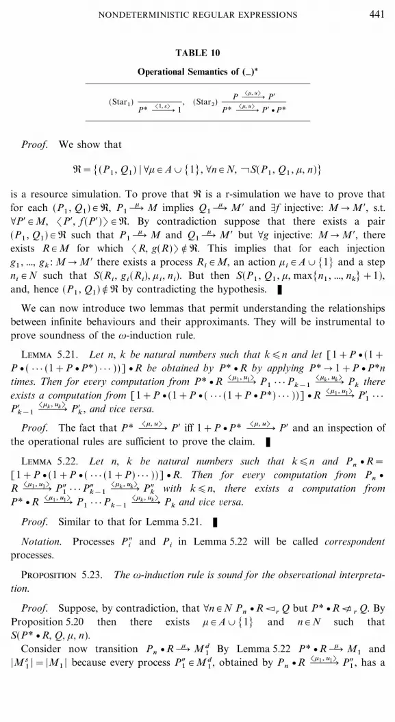
TABLE 10

Operational Semantics of (�)*

(Star1)P* ww�

(1, =)1

, (Star2)P ww�

(+, u) P$

P* ww�(+, u) P$ vP*

Proof. We show that

R=[(P1 , Q1) | \+ # A _ [1], \n # N, cS(P1 , Q1 , +, n)]

is a resource simulation. To prove that R is a r-simulation we have to prove thatfor each (P1 , Q1) # R, P1 w�+ M implies Q1 w�+ M$ and _f injective: M � M$, s.t.\P$ # M, (P$, f (P$)) # R. By contradiction suppose that there exists a pair(P1 , Q1) # R such that P1 w�+ M and Q1 w�+ M$ but \g injective: M � M$, thereexists R # M for which (R, g(R)) � R. This implies that for each injectiong1 , ..., gk : M � M$ there exists a process Ri # M, an action +i # A _ [1] and a stepni # N such that S(Ri , gi (Ri), + i , ni). But then S(P1 , Q1 , +, max[n1 , ..., nk]+1),and, hence (P1 , Q1) � R by contradicting the hypothesis. K

We can now introduce two lemmas that permit understanding the relationshipsbetween infinite behaviours and their approximants. They will be instrumental toprove soundness of the |-induction rule.

Lemma 5.21. Let n, k be natural numbers such that k�n and let [1+P v (1+P v( } } } (1+P vP*) } } } ))] vR be obtained by P* vR by applying P* � 1+P vP*ntimes. Then for every computation from P* vR ww�(+1 , u1) P1 } } } Pk&1 ww�(+k , uk) Pk thereexists a computation from [1+P v(1+P v( } } } (1+P vP*) } } } ))] vR ww�(+1 , u1) P$1 } } }P$k&1 ww�(+k , uk) P$k , and vice versa.

Proof. The fact that P* ww�(+, u) P$ iff 1+P vP* ww�(+, u) P$ and an inspection ofthe operational rules are sufficient to prove the claim. K

Lemma 5.22. Let n, k be natural numbers such that k�n and Pn vR=[1+P v(1+P v( } } } (1+P) } } } ))] vR. Then for every computation from Pn vR ww�(+1 , u1) P"1 } } } P"k&1 ww�(+k , uk) P"k with k�n, there exists a computation fromP* vR ww�(+1 , u1) P1 } } } Pk&1 ww�(+k , uk) Pk and vice versa.

Proof. Similar to that for Lemma 5.21. K

Notation. Processes Pi" and Pi in Lemma 5.22 will be called correspondentprocesses.

Proposition 5.23. The |-induction rule is sound for the observational interpreta-tion.

Proof. Suppose, by contradiction, that \n # N Pn vR Ir Q but P* vR I% r Q. ByProposition 5.20 then there exists + # A _ [1] and n # N such thatS(P* vR, Q, +, n).

Consider now transition Pn vR w�+ M d1 By Lemma 5.22 P* vR w�+ M1 and

|M s1 |=|M1 | because every process P"1 # M d

1 , obtained by Pn vR ww�(+1 , u1) P"1 , has a


(unique) correspondent P1 # M1 such that P* vR ww�(+1 , u1) P1 and vice versa. Byhypothesis Pn vR Ir Q thus Q w�+ M$1 and there exists an injection g1 : M d

1 � M$1such that for each d i

1 # M d1 , d i

1 Ir g1(d i1). Clearly g1 detects an injection

f1 : M1 � M$1 such that g1(d $)= f1(P$), where P$ # M1 is the correspondent processof d $ # M d

1 .From S(P*R, Q, +, n), it follows that there are P1 # M1 , +1 # A _ [1], n1 # N

with n1�n such that S(P1 , f1(P1), +1 , n1). Consider now P1 and the correspondentd1 in M d

1 . We have that g1(d1)= f1(P1) and d1 Ir g1(d1). Hence, d1 w�+1

M d2 and

P1 w�+1

M2 such that |M d2 |=|M2 |, because every process d i

2 # M d2 is a correspon-

dent of some process in M2 relative to the same actual (+1 , u)-transition and viceversa. From d1 Ir g1(d1) follows that g1(d1)= f1(P1) w�+1 M$2 and there exists aninjection g2 : M d

2 � M$2 such that for each d i2 # M d

2 , d i2 Ir g2(d i

2). Now g2 permitsus to detect an injection f2 : M2 � M$2 , such that g2(d $)= f2(P$) and P$ # M2 is thecorrespondent of d $ in M d

2 . Moreover since S(P1 , f1(P1), +1 , n1) there are P2 # M2 ,+2 # A _ [1], n2 # N with n2�n1 such that S(P2 , f2(P2), +2 , n2).

By following the above reasoning, we obtain dn Ir gn(dn) and S(Pn , fn(Pn),+n , 1).

Suppose now that dn w�+n M dn+1 and Pn w�+n Mn+1 with |M d

n+1 |=|Mn+1 | whereevery d i

n+1 # M dn+1 is the correspondent of some process Pn+1 # Mn+1 relative to

the same actual (+n+1 , u)-transition. By hypothesis we know that dn Ir gn(dn)and that injection gn permits to detect an injection fn : Mn � M$n , such thatgn(d $)= fn(P$) with d $ is the correspondent in M d

n of P$ # Mn . Thus, we have thatgn(dn)= fn(Pn) w�+n M$n+1 and that there exists an injection gn+1 : M d

n+1 � M$n+1

such that for each d in+1 # M d

n+1 , d in+1 Ir gn+1(d i

n+1). This contradicts the factthat S(Pn , fn(P2), +n , 1). K

Proposition 5.24 (Completeness). Axioms (C1)�(C3), (S1)�(S5), and (RD) ofTable 1, the laws of Table 4, axiom (*1) and |-induction of Table 9, soundly andcompletely axiomatize r-simulation over full PL.

Proof. Soundness of the axioms in Table 1 have been established in Section 3and of (*1) can be proved by exhibiting a simulation containing the pair(1+P vP*, P*); the proof of this exploits 5.21. Soundness of the |-induction rulehas been established in Proposition 5.23.

The completeness proof is completely similar to that given for the denotationalmodel (Theorem 5.18); obviously, in the new proof, we have to let r-simulationsplay the role that strict monomorphisms were playing in the old one. K

The proof that observational and denotational semantics are sound and completewith respect to the same set of axioms and |-induction rule, guarantees that thetwo models coincide. Actually, the proof that for each P and Q # PL we have

T�P��T�Q� iff P Ir Q

can be given in a more direct way by observing at |-induction allows us to reasonabout approximants of P with a smaller nesting degree. Again, a proof similar tothat of Theorem 5.18 is needed.


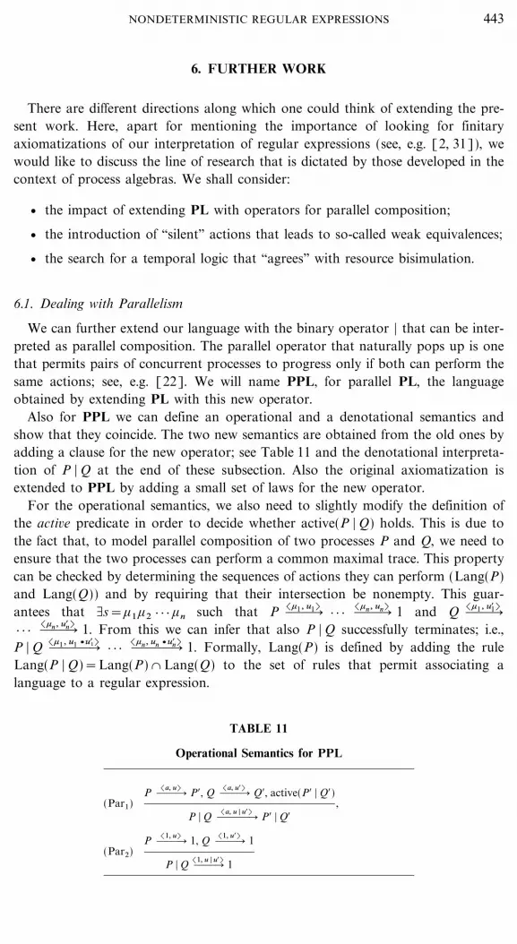
6. FURTHER WORK

There are different directions along which one could think of extending the pre-sent work. Here, apart for mentioning the importance of looking for finitaryaxiomatizations of our interpretation of regular expressions (see, e.g. [2, 31]), wewould like to discuss the line of research that is dictated by those developed in thecontext of process algebras. We shall consider:

v the impact of extending PL with operators for parallel composition;

v the introduction of ``silent'' actions that leads to so-called weak equivalences;

v the search for a temporal logic that `àgrees'' with resource bisimulation.

6.1. Dealing with Parallelism

We can further extend our language with the binary operator | that can be inter-preted as parallel composition. The parallel operator that naturally pops up is onethat permits pairs of concurrent processes to progress only if both can perform thesame actions; see, e.g. [22]. We will name PPL, for parallel PL, the languageobtained by extending PL with this new operator.

Also for PPL we can define an operational and a denotational semantics andshow that they coincide. The two new semantics are obtained from the old ones byadding a clause for the new operator; see Table 11 and the denotational interpreta-tion of P | Q at the end of these subsection. Also the original axiomatization isextended to PPL by adding a small set of laws for the new operator.

For the operational semantics, we also need to slightly modify the definition ofthe active predicate in order to decide whether active(P | Q) holds. This is due tothe fact that, to model parallel composition of two processes P and Q, we need toensure that the two processes can perform a common maximal trace. This propertycan be checked by determining the sequences of actions they can perform (Lang(P)and Lang(Q)) and by requiring that their intersection be nonempty. This guar-antees that _s=+1+2 } } } +n such that P ww�(+1 , u1) } } } ww�(+n , un) 1 and Q ww�(+1 , u$1)

} } } ww�(+n , u$n) 1. From this we can infer that also P | Q successfully terminates; i.e.,P | Q www�(+1 , u1 vu$1) } } } www�(+n , un vu$n) 1. Formally, Lang(P) is defined by adding the ruleLang(P | Q)=Lang(P) & Lang(Q) to the set of rules that permit associating alanguage to a regular expression.

TABLE 11

Operational Semantics for PPL

(Par1)P ww�

(a, u) P$, Q ww�(a, u$) Q$, active(P$ | Q$)

P | Q www�(a, u | u$) P$ | Q$

,

(Par2)P ww�

(1, u)1, Q ww�

(1, u$)1

P | Q ww�(1, u | u$)

1


TABLE 12

A Complete Set of Axioms for Parallelism

X | Y=Y | X (Par1)(X | Y) | Z=X | (Y | Z) (Par2)X | (Y+2)=X | Y+X | Z (Par3)

X | 0=0 (Par4)

+ vX | +$ vY=+ v(X | Y) if +=+$ (Par5)+ vX | +$ vY=0 if +{+$ (Par6)

1 | 1=1 (Par7)

It is possible to show that for each PPL term, P, there exists a finite stateautomata that accepts Lang(P). Moreover, the set of our languages is closed withrespect to complementation and union and it is decidable whether Lang(P) &

Lang(Q) is empty or not. This permits us to define active(P | Q) by Lang(P) &

Lang(Q){< O active(P | Q). Also for the richer language, we have a completeaxiomatization of r-simulation; the new axioms are reported in Table 12.

Proposition 6.1 (Completeness). The axioms for PL and those in Table 12completely axiomatize r-simulation over PPL.

As promised, we can provide also a denotational interpretation of the parallelcombinator. We take advantage of the following property of T.

Proposition 6.2. T has products.

Proof. Given t1=(X1 , :1 , ;1) and t2=(X2 , :2 , ;2), t1_t2=(X, :, ;) isdefined by

v X=[(x1 , x2) # X1_X2 | :1(x1)=:2(x2)]

v :((x1 , x2) )=:1(x1)=:2(x2)

v ;((x1 , x2) , ( y1 , y2) )=min(;1(x1 , y1), ;2(x2 , y2)). K

We can now extend our algebraic interpretation of PL to PPL by defining

T�P | Q�=T�P�_T�Q�

and again obtain a model for the full system of axioms.

6.2. Weak Equivalences

In this section we sketch how our work can be extended to languages withinvisible ({-)actions; i.e., we study the ``weak'' versions of resource simulation andresource bisimulation. The language PL is extended with the basic process { thatperforms the silent action { and successfully terminates:

{ ww�({, =)

1.

To define silent transitions, we will rely on a new relation [{ that permits observ-ing the branching structure of terms by ``signaling'' those states that are real choice


points, i.e. those states that have at least two active (see Table 7) alternatives. Rela-tion [{ { is used to describe the execution of consecutive { actions (possibly inter-leaved by 1's actions) with no real choice required. Clearly, we should make surethat every process of the form P+Q with cactive(Q) has [{ -transitions wheneverP has [{ -transitions. This is because we want to equate, for instance, processes{+0 and {. Using the active predicate in the definition of [{ enables us to detectsuch situations.

A weak silent transition ==O({, )

is either [{ transition (and, hence, u==), or asequence of ww�({, ui) , with choice sequence ui different from =, preceded andfollowed by [{ transitions ( [{ ww�({, ui) [{ ). In the latter case the choice sequenceis obtained by concatenating those of the involved single step transitions.

As usual a visible weak transition ===O(a, u)

is a transition ww�(a, u$) possiblypreceded and followed by invisible weak transitions. Thus,===O(a, u)

= ===O({, u1)

ww�(a, u2) ===O({, u3)

and u=u1u2u3 .To fix intuition, let us concentrate on two processes:

v P={ v{ v ({ v{ vb+{ v{ v{ vc),

v ({ v{ vb+{ v{ vc).

Process P has a single [{ -transition: P [{ ({ v{ vb+{ v{ vc) while process Q hasno [{ -transition.

Now, if we concentrate on P, we have that it has three ===O({, u)

-transitions:

1. P ==O{, =)

({ v{ vb+{ v{ vc),

2. P ===O({, l)

b,

3. P ===O({, r)

c,

and two possible ===O(a, u)

-transitions:

1. P ===O(b, l)

1,

2. P ===O(c, r)

1.

Weak resource simulation and bisimulation can be obtained by replacing w�+

with O+

in Definition 3.2; the second arrow is obtained from ===O(+, u)

just like thefirst one is obtained from ww�(+, u) .

The resulting relations will equate { v{ with { and differentiate {+{ from {. Thereason for the latter differentiation is similar to that behind 1+1t% r 1. Indeed({+{) va is equal to { va+{ va (by axiom (RD)) which has to be different (in thisnew setting) by { va.

Also weak resource simulation and bisimulation are preserved by all operators ofPL; noticeably, they are preserved by +. This is another interesting property of ourrelations. Indeed, weak equivalences are usually not preserved by + and additionalwork is needed to isolate the coarsest congruence contained in them. Here we takeadvantage of the new [{ -transition, to model initial {-moves differently than theothers.

We have completely axiomatized weak resource bisimulation over PL. The set ofaxioms is the same as that for resource bisimulation (see Table 1) with the additionof the simple {-law in Table 13 with : # A _ [{]. We would like to conclude by


TABLE 13

Axiom for Weak ResourceBisimulation

: v{ vX=: vX

remarking that Proposition 3.8 holds also in this new setting; i.e., weak resourcebisimulation is the kernel of weak resource simulation. We are still working on thecomplete axiomatization of weak resource simulation. This and the impact ofparallel and hiding operators on the weak setting will be the subject of furtherinvestigation.

6.3. Graded Modalities

A well-known result relating operational and logical semantics is that reported in[21]. In that paper, a modal logic, now known as Hennessy�Milner Logic (HML),is, defined which, when interpreted over labelled transition systems with (without)silent actions, is proved to be in full agreement with weak (strong) observationalequivalence. Other correspondences have been established in [7], where two equiv-alences over Kripke structures (node-labelled transition systems) are related to twovariants of CTL* [17], and in [16], where another variant of bisimulation calledbranching bisimulation is provided with three logical characterizations.

A logical characterization can be provided also for resource bisimulation. Thenew logics can be obtained by replacing both the box and diamond modality ofHML with a family of graded modalities [18], defined below, where * denotesmultisets cardinality,

p<(+) n � if and only if *[| p$ | p w�+ p$; p$ < �|]=n.

Now, if we define graded HML (GHML) as the set of formulae generated by thegrammar

� ::=True | False | �1 6 �2 | �1 7�2 | (+) n �,

where + is in A and 0�n<�, it can be established that

\� # GHML, P < � � Q < � if and only if Ptr Q.

7. CONCLUSION AND RELATED WORKS

Regular expressions have been the subject of many investigations since the earlyfifties. By now, they have three standard equivalent semantics that represent alter-native ways of capturing the fact that regular expressions are a natural and com-pact notation for describing sets of (alternative) sequential behaviors of systems.Regular expressions have been equipped with:


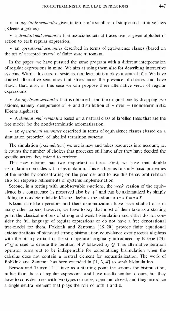
v an algebraic semantics given in terms of a small set of simple and intuitive laws(Kleene algebras);

v a denotational semantics that associates sets of traces over a given alphabet ofaction to each regular expression;

v an operational semantics described in terms of equivalence classes (based onthe set of accepted traces) of finite state automata.

In the paper, we have pursued the same program with a different interpretationof regular expressions in mind. We aim at using them also for describing interactivesystems. Within this class of systems, nondeterminism plays a central role. We havestudied alternative semantics that stress more the presence of choices and haveshown that, also, in this case we can propose three alternative views of regularexpressions:

v An algebraic semantics that is obtained from the original one by dropping twoaxioms, namely idempotence of + and distribution of v over + (nondeterministicKleene algebras);

v A denotational semantics based on a natural class of labelled trees that are thefree model for the nondeterministic axiomatization;

v an operational semantics described in terms of equivalence classes (based on asimulation preorder) of labelled transition systems.

The simulation (r-simulation) we use is new and takes resources into account; i.e.it counts the number of choices that processes still have after they have decided thespecific action they intend to perform.

This new relation has two important features. First, we have that doubler-simulation coincides with r-bisimulation. This enables us to study basic propertiesof the model by concentrating on the preorder and to use this behavioral relationalso for stepwise refinements of systems implementation.

Second, in a setting with unobservable {-actions, the weak version of the equiv-alence is a congruence (is preserved also by +) and can be axiomatized by simplyadding to nondeterministic Kleene algebras the axiom: : v{ vX=: vX.

Kleene star-like operators and their axiomatization have been studied also inmany other papers; however, we have to say that most of them take as a startingpoint the classical notions of strong and weak bisimulation and either do not con-sider the full language of regular expressions or do not have a free denotationaltree-model for them. Fokkink and Zantema [19, 20] provide finite equationalaxiomatizations of standard strong bisimulation equivalence over process algebraswith the binary variant of the star operator originally introduced by Kleene (23).P*Q is used to denote the iteration of P followed by Q. This alternative iterationoperator turns out to be indispensable for axiomatizing bisimulation when thecalculus does not contain a neutral element for sequentialization. The work ofFokkink and Zantema has been extended in [1, 3, 4] to weak bisimulation.

Benson and Tiuryn [11] take as a starting point the axioms for bisimulation,rather than those of regular expressions and have results similar to ours, but theyhave to consider trees with two types of nodes, open and closed, and they introducea single neutral element that plays the role of both 1 and 0.


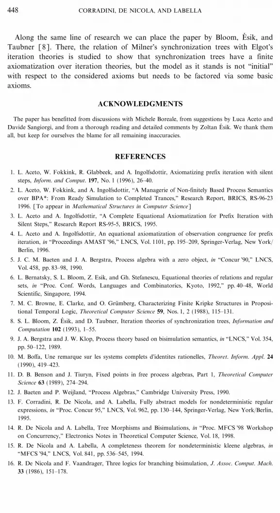
Along the same line of research we can place the paper by Bloom, E� sik, andTaubner [8]. There, the relation of Milner's synchronization trees with Elgot'siteration theories is studied to show that synchronization trees have a finiteaxiomatization over iteration theories, but the model as it stands is not `ìnitial''with respect to the considered axioms but needs to be factored via some basicaxioms.

ACKNOWLEDGMENTS

The paper has benefitted from discussions with Michele Boreale, from suggestions by Luca Aceto andDavide Sangiorgi, and from a thorough reading and detailed comments by Zoltan E� sik. We thank themall, but keep for ourselves the blame for all remaining inaccuracies.

REFERENCES

1. L. Aceto, W. Fokkink, R. Glabbeek, and A. Ingolfsdottir, Axiomatizing prefix iteration with silentsteps, Inform. and Comput. 197, No. 1 (1996), 26�40.

2. L. Aceto, W. Fokkink, and A. Ingolfsdottir, `À Managerie of Non-finitely Based Process Semanticsover BPA*: From Ready Simulation to Completed Trances,'' Research Report, BRICS, RS-96-231996. [To appear in Mathematical Structures in Computer Science]

3. L. Aceto and A. Ingolfsdottir, `À Complete Equational Axiomatization for Prefix Iteration withSilent Steps,'' Research Report RS-95-5, BRICS, 1995.

4. L. Aceto and A. Ingolfsdottir, An equational axiomatization of observation congruence for prefixiteration, in ``Proceedings AMAST '96,'' LNCS, Vol. 1101, pp. 195�209, Springer-Verlag, New York�Berlin, 1996.

5. J. C. M. Baeten and J. A. Bergstra, Process algebra with a zero object, in ``Concur '90,'' LNCS,Vol. 458, pp. 83�98, 1990.

6. L. Bernatsky, S. L. Bloom, Z. Esik, and Gh. Stefanescu, Equational theories of relations and regularsets, in ``Proc. Conf. Words, Languages and Combinatorics, Kyoto, 1992,'' pp. 40�48, WorldScientific, Singapore, 1994.

7. M. C. Browne, E. Clarke, and O. Gru� mberg, Characterizing Finite Kripke Structures in Proposi-tional Temporal Logic, Theoretical Computer Science 59, Nos. 1, 2 (1988), 115�131.

8. S. L. Bloom, Z. E� sik, and D. Taubner, Iteration theories of synchronization trees, Information andComputation 102 (1993), 1�55.

9. J. A. Bergstra and J. W. Klop, Process theory based on bisimulation semantics, in ``LNCS,'' Vol. 354,pp. 50�122, 1989.

10. M. Boffa, Une remarque sur les systems complets d'identites rationelles, Theoret. Inform. Appl. 24(1990), 419�423.

11. D. B. Benson and J. Tiuryn, Fixed points in free process algebras, Part 1, Theoretical ComputerScience 63 (1989), 274�294.

12. J. Baeten and P. Weijland, ``Process Algebras,'' Cambridge University Press, 1990.

13. F. Corradini, R. De Nicola, and A. Labella, Fully abstract models for nondeterministic regularexpressions, in ``Proc. Concur 95,'' LNCS, Vol. 962, pp. 130�144, Springer-Verlag, New York�Berlin,1995.

14. R. De Nicola and A. Labella, Tree Morphisms and Bisimulations, in ``Proc. MFCS '98 Workshopon Concurrency,'' Electronics Notes in Theoretical Computer Science, Vol. 18, 1998.

15. R. De Nicola and A. Labella, A completeness theorem for nondeterministic kleene algebras, in``MFCS '94,'' LNCS, Vol. 841, pp. 536�545, 1994.

16. R. De Nicola and F. Vaandrager, Three logics for branching bisimulation, J. Assoc. Comput. Mach.33 (1986), 151�178.


17. E. H. Emerson and Y. Halpern, ``Sometimes'' and ``not never'' revisited: On branching versus lineartime temporal logic, Journal of ACM 42 (1995), 458�487.

18. M. Fattorosi-Barnaba and F. De Caro, Graded Modalities, I; Studia Logica 44 (1985), 197�221.

19. W. Fokkink, A complete equational axiomatization for prefix iteration, Inform. Process. Lett. 52(1994), 333�337.

20. W. Fokkink and H. Zantema, Basic process algebra with iteration: completeness of its equationalaxioms, Comput. J. 37 (1994), 259�267.

21. M. Hennessy and R. Milner, Algebraic Laws for Nondeterminism and Concurrency, J. Assoc.Comput. Mach. 32 (1985), 137�161.

22. C. A. R. Hoare, ``Communicating Sequential Processes,'' Prentice�Hall, Englewood Cliffs, NJ, 1989.

23. S. C. Kleene, Representation of Events in Nerve Nets and Finite Automata, in `Àutomata Studies''(Shannon and McCarthy, Eds.), pp. 3�41, Princeton Univ. Press, 1956.

24. S. Kasangian and A. Labella, Enriched Categorical Semantics for Distributed Calculi, J. Pure Appl.Algebra 83 (1992), 295�321.

25. D. Kozen, A completeness theorem for kleene algebras and the algebra of regular events, Informationand Computation 110 (1994), 366�390.

26. D. Krob, Complete systems of B-rational identities, Theoretical Computer Science 89 (1991),207�343.

27. R. Milner, ``Communication and Concurrency,'' Prentice�Hall, 1989.

28. D. Park, Concurrency and automata on infinite sequences, in ``Proc. GI,'' LNCS, Vol. 104,pp. 167�183, 1981.

29. B. C. Pierce, ``Basic Category Theory for Computer Scientists,'' The MIT Press, Cambridge, MA,1991.

30. A. Salomaa, Two complete axiom systems for the algebra of regular events, Journal of ACM 13(1966), 158�169.

31. P. Sewell, Bisimulation is not finitely (first order) equationally axiomatisable, in ``Proc. of LICS,''IEEE Press, 1994.

32. M. B. Smith and G. D. Plotkin, The category-theoretic solution of recursive domain equation,J. Comput. 11 (1982), 762�783.


Models of Nondeterministic Regular Expressions

Documents