UNIVERSITATIS OULUENSIS ACTA C TECHNICA OULU 2011 C 379 Juha Kalliokoski MODELS OF FILTRATION CURVE AS A PART OF PULP DRAINAGE ANALYZERS UNIVERSITY OF OULU, FACULTY OF TECHNOLOGY, DEPARTMENT OF ELECTRICAL AND INFORMATION ENGINEERING C 379 ACTA Juha Kalliokoski

Welcome message from author
This document is posted to help you gain knowledge. Please leave a comment to let me know what you think about it! Share it to your friends and learn new things together.
Transcript

ABCDEFG
UNIVERS ITY OF OULU P.O.B . 7500 F I -90014 UNIVERS ITY OF OULU F INLAND
A C T A U N I V E R S I T A T I S O U L U E N S I S
S E R I E S E D I T O R S
SCIENTIAE RERUM NATURALIUM
HUMANIORA
TECHNICA
MEDICA
SCIENTIAE RERUM SOCIALIUM
SCRIPTA ACADEMICA
OECONOMICA
EDITOR IN CHIEF
PUBLICATIONS EDITOR
Senior Assistant Jorma Arhippainen
Lecturer Santeri Palviainen
Professor Hannu Heusala
Professor Olli Vuolteenaho
Senior Researcher Eila Estola
Director Sinikka Eskelinen
Professor Jari Juga
Professor Olli Vuolteenaho
Publications Editor Kirsti Nurkkala
ISBN 978-951-42-9426-6 (Paperback)ISBN 978-951-42-9427-3 (PDF)ISSN 0355-3213 (Print)ISSN 1796-2226 (Online)
U N I V E R S I TAT I S O U L U E N S I SACTAC
TECHNICA
U N I V E R S I TAT I S O U L U E N S I SACTAC
TECHNICA
OULU 2011
C 379
Juha Kalliokoski
MODELS OF FILTRATION CURVE AS A PART OF PULP DRAINAGE ANALYZERS
UNIVERSITY OF OULU,FACULTY OF TECHNOLOGY,DEPARTMENT OF ELECTRICAL AND INFORMATION ENGINEERING
C 379
ACTA
Juha Kalliokoski
C379etukansi.kesken.fm Page 1 Tuesday, April 19, 2011 10:09 AM


A C T A U N I V E R S I T A T I S O U L U E N S I SC Te c h n i c a 3 7 9
JUHA KALLIOKOSKI
MODELS OF FILTRATION CURVE AS A PART OF PULP DRAINAGE ANALYZERS
Academic dissertation to be presented with the assent ofthe Faculty of Technology of the University of Oulu forpublic defence in OP-sali (Auditorium L10), Linnanmaa, on3 June 2011, at 12 noon
UNIVERSITY OF OULU, OULU 2011
Copyright © 2011Acta Univ. Oul. C 379, 2011
Supervised byProfessor Risto Myllylä
Reviewed byProfessor Jouko HalttunenProfessor Alexander V. Priezzhev
ISBN 978-951-42-9426-6 (Paperback)ISBN 978-951-42-9427-3 (PDF)http://herkules.oulu.fi/isbn9789514294273/ISSN 0355-3213 (Printed)ISSN 1796-2226 (Online)http://herkules.oulu.fi/issn03553213/
Cover DesignRaimo Ahonen
JUVENES PRINTTAMPERE 2011
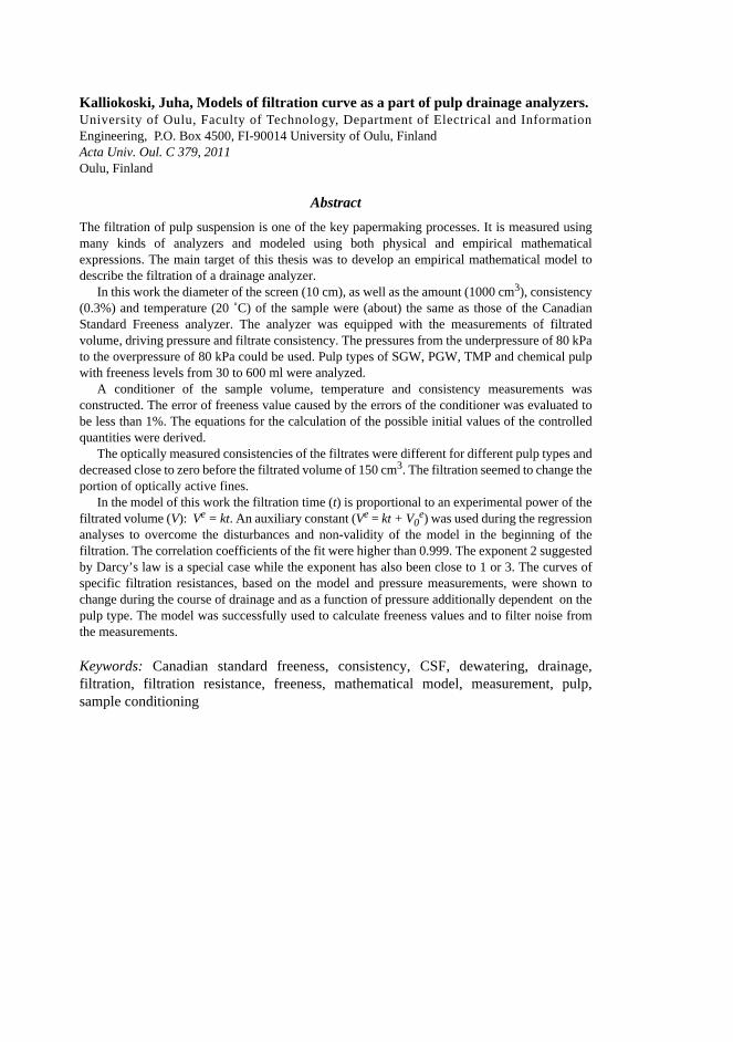
Kalliokoski, Juha, Models of filtration curve as a part of pulp drainage analyzers. University of Oulu, Faculty of Technology, Department of Electrical and InformationEngineering, P.O. Box 4500, FI-90014 University of Oulu, FinlandActa Univ. Oul. C 379, 2011Oulu, Finland
AbstractThe filtration of pulp suspension is one of the key papermaking processes. It is measured usingmany kinds of analyzers and modeled using both physical and empirical mathematicalexpressions. The main target of this thesis was to develop an empirical mathematical model todescribe the filtration of a drainage analyzer.
In this work the diameter of the screen (10 cm), as well as the amount (1000 cm3), consistency(0.3%) and temperature (20 ˚C) of the sample were (about) the same as those of the CanadianStandard Freeness analyzer. The analyzer was equipped with the measurements of filtratedvolume, driving pressure and filtrate consistency. The pressures from the underpressure of 80 kPato the overpressure of 80 kPa could be used. Pulp types of SGW, PGW, TMP and chemical pulpwith freeness levels from 30 to 600 ml were analyzed.
A conditioner of the sample volume, temperature and consistency measurements wasconstructed. The error of freeness value caused by the errors of the conditioner was evaluated tobe less than 1%. The equations for the calculation of the possible initial values of the controlledquantities were derived.
The optically measured consistencies of the filtrates were different for different pulp types anddecreased close to zero before the filtrated volume of 150 cm3. The filtration seemed to change theportion of optically active fines.
In the model of this work the filtration time (t) is proportional to an experimental power of thefiltrated volume (V): Ve = kt. An auxiliary constant (Ve = kt + V0
e) was used during the regressionanalyses to overcome the disturbances and non-validity of the model in the beginning of thefiltration. The correlation coefficients of the fit were higher than 0.999. The exponent 2 suggestedby Darcy’s law is a special case while the exponent has also been close to 1 or 3. The curves ofspecific filtration resistances, based on the model and pressure measurements, were shown tochange during the course of drainage and as a function of pressure additionally dependent on thepulp type. The model was successfully used to calculate freeness values and to filter noise fromthe measurements.
Keywords: Canadian standard freeness, consistency, CSF, dewatering, drainage,filtration, filtration resistance, freeness, mathematical model, measurement, pulp,sample conditioning


Kalliokoski, Juha, Suodoskäyrän mallit suotautuvuusanalysaattorien osana. Oulun yliopisto, Teknillinen tiedekunta, Sähkö- ja tietotekniikan osasto, PL 4500, 90014 OulunyliopistoActa Univ. Oul. C 379, 2011Oulu
TiivistelmäPaperimassasulpun suotauttaminen on paperinvalmistuksen avainprosesseja. Sitä on mitattumonenlaisilla analysaattoreilla ja kuvattu sekä fysikaalisilla että kokeellisilla matemaattisillamalleilla. Tämän tutkimuksen päätavoite on kehittää suotautuvuusanalysaattorin kokeellistamatemaattista mallia.
Tutkimuksessa viiran halkaisija (10 cm) sekä näytteen määrä (1000 cm3), sakeus (0.3 %) jalämpötila (20 ˚C) olivat suunnilleen samat kuin Canadian standard freeness –analysaattorissa.Järjestelmä mittasi suotautettua tilavuutta, suotauttavaa painetta ja suodoksen sakeutta. Suotau-tuspaineet olivat 80 kPa:n ali- ja ylipaineen väliltä. Testattavana oli hioketta, painehioketta jatermohierrettä sekä kemiallista massaa, joiden freeness oli 30 ml:sta 600 ml:aan.
Analysaattoriin rakennettu vakiointijärjestelmä sääti näytteen sakeuden, tilavuuden ja lämpö-tilan niin tarkasti halutuiksi, että näiden vaihtelu ei olisi muuttanut freeness-arvoa edes prosent-tia. Suureiden kehittymiselle johdettiin kaavat. Niiden avulla voidaan laskea ne näytteen arvo-alueet, joilta halutut tavoitearvot voidaan saavuttaa.
Optisesti mitattu suodoksen sakeus riippui massatyypistä ja hiipui lähes nollaksi ennen kuin150 ml oli suotautettu. Suotautus muutti optisesti aktiivisen hienoaineen osuutta.
Tämän työn suodoskäyrän mallissa aika (t) on verrannollinen suotautetun tilavuuden (V)kokeellisen potenssiin: Ve = kt. Mallinnuksen ajaksi lisätään apuparametri (Ve = kt+V0
e), jottasuotautuksen alku ei huononna mallia. Sovituksen korrelaatiokerroin oli yli 0.999. Eksponentinarvo vaihteli vähän yli yhdestä melkein kolmeen, joten Darcyn lain mukainen eksponentin arvo2 osoittautui erikoistapaukseksi. Mallin ja painemittauksen avulla lasketut ominaisresistanssitmuuttuivat suotautuksen kuluessa ja riippuivat myös massatyypistä. Mallin avulla voitiin laskeanäytteen freeness sekä suodattaa mittauskohinaa.
Asiasanat: analysaattori, Canadian standard freeness, CSF, freeness, matemaattinenmalli, mittaus, näytteen vakiointi, paperimassa, sakeus, suotautus, suotautusvastus,suotautuvuus


7
Acknowledgements
This thesis is based on research carried out at Kajaani Polytechnic during the years 1989–1998 and in the Measurement and Sensor Laboratory, University of Oulu, during the years 1998–2010. The work was financed by the Kainuu Regional Fund of the Finnish Cultural Foundation, the Finnish Foundation for Technology Promotion and the Jenny and Antti Wihuri Foundation.
I wish to express my sincere gratitude to my supervisor Professor Risto Myllylä for his unwavering and persistent guidance and encouragements throughout the work – as well as to Professor Matti Karras for his inspiring and foresighted indications towards the target of this research. I am grateful to the reviewers of this thesis, Professor Alexander V. Priezzhev from M.V. Lomonosov Moscow State University and Professor Jouko Halttunen from Tampere University of Technology for their numerous polishing remarks. I want to thank M.Sc. Aaron Bergdahl for revising the English and M.Sc. Niina Sarajärvi the Finnish language of the manuscript.
I wish to express my warm thanks to the Rector of Kajaani Polytechnic, Risto Hurttia who kindly urged me to exploit the facilities of the laboratories and to the personnel of the school: engineers Risto Janhila and Markku Sinisalo and especially to the very skilful and innovative technician Ilpo Saren. I would like to thank the companies UPM (Kymmene) and Valmet Automation (Metso) and their staff for the absolutely necessary material and conceptual help.
I am forever grateful to my family and the friends close to me for their unselfish support and patience during the long trek of this work.
Kajaani, February 2011 Juha Kalliokoski

8

9
Abbreviations and symbols
CSF Canadian standard freeness CTMP chemithermomechanical pulp DDA Dynamic Drainage Analyzer DDJ Dynamic Drainage Jar KRAFT chemical pulp LC -100 Kajaani low consistency transmitter LCF low consistency meter tailored for this work LCFM measurement signal of LCF (shortly M) LCFR reference signal of LCF (shortly R) MBDT Moving Belt Drainage Tester PDA Pulp Drainage Analyzer PDAX Pulp Drainage Analyzer tailored for this work PDAY Pulp Drainage Analyzer tailored for this work PGW pressurized groundwood Pt-100 resistive temperature sensor RS-filter 1st order low pass frequency filter SGW stone groundwood SR Schopper Riegler freeness TMP thermomechanical pulp WRC water retention value A area ch specific heat capacity C consistency, mass of solids per mass of slurry C0 initial consistency (of the sample in conditioning or in drainage) C1 consistency when the target mass is reached in the conditioner Cf fines content CM consistency of fiber mat, mass of solids per total mass Cm solid content of fiber mat, mass of solids per total volume CSF value of canadian standard freeness CSFC calculated value of CSF Ct consistency target of the conditioner CV volume fraction of solids, volume of solids per volume of mat
10
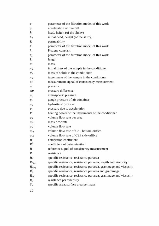
e parameter of the filtration model of this work g acceleration of free fall h head, height (of the slurry) h0 initial head, height (of the slurry) K permeability k parameter of the filtration model of this work k Kozeny constant kL parameter of the filtration model of this work L length m mass m0 initial mass of the sample in the conditioner mk mass of solids in the conditioner mt target mass of the sample in the conditioner M measurement signal of consistency measurement p pressure Δp pressure difference pa atmospheric pressure pc gauge pressure of air container ph hydrostatic pressure pr pressure due to acceleration P heating power of the instruments of the conditioner qA volume flow rate per area qm mass flow rate qV volume flow rate qV1 volume flow rate of CSF bottom orifice qV2 volume flow rate of CSF side orifice R correlation coefficient R2 coefficient of determination R reference signal of consistency measurement R resistance RA specific resistance, resistance per area RALη specific resistance, resistance per area, length and viscocity RAWη specific resistance, resistance per area, grammage and viscosity RS specific resistance, resistance per area and grammage RSη specific resistance, resistance per area, grammage and viscosity Rη resistance per viscosity Sm specific area, surface area per mass

11
SV specific area, surface area per volume t time t1 time when flow of CSF side orifice stops t1 time when the target mass in the conditioner is reached t1/2 period of decay of the consistency in the conditioner tn sampling time of sample no. n T temperature T1 temperature when the target mass in the conditioner is reached T∞ asymptotic temperature of the conditioner TEARC calculated tear strength TENSC calculated tensile strength Te1 temperature constant of the model of the conditioning Tt temperature target of conditioner TV temperature of dilution and cooling water of the conditioner u velocity (of the surface of the sample) V volume V0 initial volume (of the sample) V0
e parameter of the filtration model of this work V2 volume that has flown out of the CSF side orifice VC volume of the CSF bottom cone Vn measured volume of sample no. n W basis weight, grammage, mass per area ε porosity εmax maximum porosity in a pad εmin minimum porosity in a pad η dynamic viscosity ν specific volume ρ density τ time constant of the conditioner . decimal separator , decimal separator

12

13
Contents
Abstract Tiivistelmä Acknowledgements 7 Abbreviations and symbols 9 Contents 13 1 Introduction 15
1.1 Objectives of the thesis ........................................................................... 17 1.2 Contributions to the thesis ....................................................................... 18 1.3 Structure of the thesis .............................................................................. 18
2 Dewatering processes in paper making 21 2.1 Pulping processes .................................................................................... 21 2.2 Forming process ...................................................................................... 22
3 Measurement of drainability 25 3.1 Matters that influence drainage measurements ....................................... 25 3.2 Pioneers of freeness testers ..................................................................... 26 3.3 Freeness and slowness testers ................................................................. 27
4 Models of drainage 31 4.1 Physical background of dewatering ........................................................ 31 4.2 Physical mathematical models of dewatering ......................................... 33 4.3 Empirical mathematical models of dewatering ....................................... 37 4.4 Models of freeness testers ....................................................................... 45
5 Experimental arrangements 49 6 The sample conditioner 55
6.1 Construction and working principle of the conditioner ........................... 55 6.2 Theoretical progress of the conditioning ................................................. 56
6.2.1 Conditioning of consistency ......................................................... 57 6.2.2 Conditioning of temperature ......................................................... 59 6.2.3 Theoretical temperature and consistency limits for the
conditioned sample ....................................................................... 61 6.3 Conditioning experiments ....................................................................... 62
7 Applied model 65 7.1 Model of filtration curve ......................................................................... 67 7.2 Filtration flow ......................................................................................... 68 7.3 Superficial velocity ................................................................................. 68 7.4 Filtration resistance ................................................................................. 69

14
7.5 Uniform drainage .................................................................................... 71 7.6 Logarithmic filtration curves ................................................................... 72 7.7 Solving the parameters of the filtration curve ......................................... 72
8 Fitting to the measurements 75 8.1 Used fitting method ................................................................................. 75 8.2 Quality of the fit of the model and the measurement .............................. 76 8.3 Experimentally obtained models of filtration curves .............................. 77
8.3.1 Mutual relations between the two parameters of the model ......... 79 8.3.2 Repeatability of the filtration curves ............................................ 83
8.4 Alternative means to fit the model to the measurements ........................ 85 9 Experimental models of resistance 95
9.1 Filtrating pressure .................................................................................... 96 9.2 Trends of the specific resistance.............................................................. 98 9.3 The model as a noise filter .................................................................... 101
10 Models of freeness and strength of pulp 103 11 Consistency of filtrate 109 12 Discussion 117 13 Summary 121 References 123 Appendices 127

15
1 Introduction
The interaction between fibers and water is one of the most basic phenomena in paper physics and dewatering is one of the main operations in the papermaking process.
Water has strong effects on the external shape and the internal structure of individual fibers and thereby also on many important physical and other papermaking properties of fibers.
Water is also necessary in linking as well as separating fibers. Water has an important role in the separation of fibers from wood material
and from each other with the help of chemicals, heat or mechanical treatment. Water is needed when finishing the properties of pulp in refiners for different types of paper products; one of those properties is the water-fiber interaction itself.
Water is separated from the rest of pulp suspension ( slurry or stuff or furnish or stock) in many stages of the papermaking process, for instance in washing after cooking and bleaching, in thickening before bleaching, screening and finally in filtration on the paper machine wire, which is perhaps the most crucial piece of process to fix the properties of paper, rate of production and energy consumption of paper production. The ability of pulp to drain water from the pulp slurry through the wire is called freeness. Water is also removed by vaporizing in many processes like in the hot pulping conditions of thermomechanical or TMP refiner and in the paper machine.
Undoubtedly, a deep understanding of the behavior of water in pulp slurries is of greatest importance for both paper scientists and paper engineers.
Numerous distinguished scientific experiments have been done to connect paper physics and drainage processes – both to predict drainage when the basic physical properties of pulp are known and to find out physical quantities by measuring drainage. In spite of the fact that the physical models of drainability are very sophisticated and their mathematical formulas very complicated, it is usually expected that drainage follows Darcy's law. In many cases this is a good enough assumption but sometimes a more precise model might be welcome. Many graphs of this work show visually that the measured filtration curves are more or less curvy than the curve suggested by Darcy’s law: the decreasing of the filtration flow rate as a function time seems to be different for different pulp types. This curvature and differences of it are described by a numerical parameter presented in this thesis.

16
On the other hand many kinds of measurement devices have been made and used for practical process control purposes. Many kinds of devices are needed because of the great variety of dewatering processes. Besides being used to predict and control dewatering processes the drainage meters are used to indirectly control many other pulp quality properties because they develop hand in hand with drainability in some processes like in refiners. So drainability is a kind of general measure for pulp quality; other quantities are often compared on the same freeness level. These practical testers give one figure to describe the drainability of pulp but unfortunately the figure is equally dependent on the measurement device and on the pulp itself. One tailored figure is especially questionable when used to describe quantities other than drainability. Additionally, the variety of different types of pulps, processes and conditions is enormous. Though a unique drainability theory, quantity and measurement device have frequently been needed and some of them now and then also offered, many sorts of quantities and devices are still used. Perhaps the basic water-fiber interaction is so complicated and its process applications so different that several kinds of descriptions will always be necessary. Thus, in many cases process operators and engineers – even salesmen of pulp – are happy with these special quantities.
General links are however needed to connect the many drainability quantities to each other and also to paper physics. A proposal for such a link is presented in this thesis. It is a mathematical formula used to describe the course of free water removal – more precise than the widely used Darcy's law but simple enough for practical on-line analyzers.
All possible sorts of mathematical formulas have surely been used earlier to describe filtration. This is also true of the formulas examined in this thesis. The main mathematical formula of this work has been presented by Wahlström and O’Blenes in 1962, but surprisingly not reported after that. Apparently the focus of that work has not been very fruitful. The purpose of the formula has been to propose two new quantities to describe the quality of pulp. Since then the technology and needs have totally changed. Thus, new possibilities to utilize this model may have arisen.
Anyhow more knowledge about and new perspectives to water removal from pulp slurries is most welcome – surely also from the signal processing point of view; one piece of that is offered by this thesis.

17
1.1 Objectives of the thesis
The main target of this thesis is to show how useful an empirical mathematical model of a filtration curve could be as a component of pulp drainage analyzers.
The following additional challenges are also included as part of this research work.
The correlation of this model with the measured curve must be clearly better than that of Darcy's law and typically in the calibration of commercial on-line drainage analyzers.
The model should be valid across a wide range of pulp types, grammages (or basis weights or masses per square meter) and driving pressures.
The mathematical formula of the model must be simple including only two parameters which must be able to be determined using any common linear regression analysis program.
The model could also be used to filter out random noise of drainage measurement without corrupting the shape of the drainage curve as much as by simple time averaging or RC-filtering.
The model will be used to calculate other drainability quantities like the filtration resistance and the most common freeness quantities, Canadian Standard Freeness (CSF) values of the pulp samples.
All these results should be achieved using robust on-line process measurement technology – without the need of precision analyzers or components.
Additionally the driving pressure was measured as a function of time. So the filtration resistances were able to be calculated in order to see how this variable is dependent on pulp types, pressures and phase of filtration.
Some optical properties of filtrate were also measured to detect possible differences of retention between pulp types and driving pressures as well as during the course of drainage.
Could these measurements together indicate if the increase of resistance is due to compression caused by the driving pressure or due to inserting material into the fiber mat by the slurry flow?
Possibilities of automatic control of the volume, consistency and temperature of the sample were also examined in order to overcome the main disturbances of drainage analyzers. The error of the freeness-value caused by these three quantities should be insignificant after this conditioning.
18
1.2 Contributions to the thesis
The scientific core of this thesis is to yield new knowledge about the use of mathematical models of the pulp drainage curve as a part of pulp drainage analyzers.
Two measurement systems for this work were constructed based on the commercial Kajaani PDA analyzer. The wire chamber remained unchanged but extra accessories were built for controlling the temperature and consistency of the sample, using pressures from 80 kPa below the atmospheric pressure to the overpressure of 80 kPa and for continuously measuring the pressure, filtration curve and optical absorption of filtrate. These new properties were specified by the author and the equipment was constructed mainly by Valmet Automation. The automatic sample conditioning system was however both planned as well as constructed by the author. This conditioner was the only part of equipment which was intended to be more precise than the original commercial tester, while the benefit of the filtration model was due to be seen using the untrimmed technology. One contribution of this thesis is showing how the automatic control of the sample can be used to improve the freeness analyzer.
Pulp samples and their laboratory analyses were supplied by the UPM Kajaani paper mill; sample sets were planned by the author together with the representatives of the paper mill. Most of the routine measurements using the experiment analyzer were made by assistants Risto Janhila and Markku Sinisalo according to detailed guidance from the author. All the data analyses were made by the author.
It has turned out that the mathematical expression of the drainage curve which is used in this thesis has earlier been used in one research work in 1962 (Wahlström & O’Blenes 1962). However, it has also turned out that the model is worth reviving for new scientific examination – for heavy factory work as well. In our work an auxiliary parameter is added to the model to overcome the modeling problems in the beginning of filtration. A wider range of driving pressures, pulp types and grammages was used to show the validity of our model. In our work the use of the model as a noise filter was also examined.
1.3 Structure of the thesis
This thesis is written keeping in mind that the target groups are the specialists of both applied electronics and process technology.

19
The general importance of the scope of this work is evaluated and the author’s contribution to the work is described in the beginning of this thesis (Chapter 1). The industrial application surrounding is described starting from the outlines of the papermaking process (Chapter 2), concentrating on the measurement technology of the quantities close to this work (Chapter 3) and finally focusing on the mathematical models of the target processes, analyzers and phenomena (Chapter 4).
The research arrangements are presented (Chapter 5) before the experimental results and the mathematical modeling of sample conditioning (Chapter 6), filtration curves (Chapters 7–9, 11) and freeness (Chapter 10).
The results of the work are discussed regarding the usefulness as well as the guidelines for the further research of this topic (Chapter 12), and the main results of the thesis finally summarized (Chapter 13).

20

21
2 Dewatering processes in paper making
The main raw material of paper is wood fibers (Niskanen et al. 1988: 14). The accompaniment of water is of vital importance in (all) paper making processes (Clark 1985: 170, Ebeling 1983). Besides these two permanent components the pulp slurry consists of many kinds of chemicals, additives, fillers, etc., the portions of which change during the course of time and process. Growing trees consist of as much water as solid material, and between harvesting and processing one must maintain the moisture content of wood material, e.g. by spraying water on the logs stored on the yards of paper mills. Additional water is needed in the debarking drums. (Biermann 1996: 18–23) Lignin is an organic compound that connects the wood fibers and is responsible for providing mechanical strength to the main stems of trees, the structure that transports water from the roots to the crown of the tree.(Biermann 1996: 36, Clark 1985: 116–118, Seppälä et al. 1999: 75). This construction remains undamaged after being cut into chips, which are a couple of millimeters thick and the area of which is a couple of square centimeters (Koskinen 2000: 369–377, Seppälä et al. 1999: 31).
2.1 Pulping processes
The fibers are separated using two main principles – mechanical and chemical pulping. Water is necessary for both of these. Grinding is one of the two main mechanical pulping methods. The logs are not chipped before this process. A pile of one meter to one and a half meter long logs are pressed against a rotating cylindrical “stone” so that the axes of both the grinding stone and logs are parallel. The rough surface of the stone warms and thereby softens the lignin between the fibers making it easier to remove the fibers layer by layer from the surface of the logs. Water is needed as a lubricant between the stone and logs, to conduct heat into the log, buffer and mediate the temperature and finally to transport the fibers, stone groundwood (SGW) pulp out of the grinder. When the grinder is pressurized, a temperature higher than 100 oC can be used in grinding (without vaporizing the necessary water out of the grinding zone) and less mechanical force is needed to comb the fibers from the logs. Pressurized groundwood (PGW) pulp is produced by this means. (Biermann 1996: 64–67)
Another type of mechanical pulp is thermomechanical pulp (TMP). Logs are first chopped into chips (Koskinen 2000: 369–377, Seppälä et al. 1999: 31) and warmed using hot steam before being fed into the pressurized refiner. Between

22
the grooved surfaces of the rotating metal plates the chips are gradually turned into the separate fibers. (Biermann 1996:. 67–69)
In the chemical pulping process, the lignin is dissolved into different kinds of water solutions (Gullichsen 2000: A28) and is then displaced by water. In these washing processes the liquids are forced to move through the net of fibers - an operation that is close to the scope of this work. The cooking is usually complemented by another chemical treatment, bleaching, in order to improve the brightness of the pulp and the final paper product. (Pikka et al. 2000) And once again the spent liquid as well as the displacing water, must be transported through a fiber bed. After cooking the fibers can be separated by the most gentle mechanical treatment (Gullichsen 2000: A28), but they are finished for different types of papers in refiners (Lumiainen 2000).
Mechanical pulps are often bleached too. This is not only accomplished by removing darkening material (through the fiber mat) from the pulp but also by changing their brightness by using chemicals. Before certain types of bleaching processes plenty of water must be pressed through the pulp pad in order to increase the consistency of pulp. (Lindholm 1999: 313, 325)
There are also some other pulping methods e.g. the chemical treatments of which can be “lighter” connected with the mechanical ones heavier than those of chemical pulps. But these chemithermomechanical pulps (CTMP) are not used in this work. Pulps based on fibers other than wooden or recycled fibers do not fall within the scope of this thesis.
Water and solid particles are separated, e.g. in screens and cleaners, too. Air is also removed from the paper mill liquids and air may affect the filtration resistance.
2.2 Forming process
The very final removal of water happens in the paper machine, which can be divided into wire, press and dryer sections (Fig. 1). The stock, a fibrous water mixture is fed from the headbox through its slice or nozzles on the moving wire or between two wires through which liquid with some fines are filtrated and on which a mat, a wet web, is forming. Many kinds of dewatering elements create pressure pulses that vibrate and partly deflocculate the fibers while water is removed. The concentration is typically increased on the wire from 0.2 … 1.2% to 20%. Next, the press section removes water from the web into endless felts by pressing in the nips between the rolls. The felt runs around a closed loop and is

23
dewatered by suction boxes while not in contact with the web outside the nip of the press rolls. After the press section the solids content may be 35–50% (about the same as in a growing tree). The rest of the water must be vaporized from the web in the dryer section. (Norman 2000)
Fig. 1. Schematic illustration of a fourdrinier former (Norman 2000, published by
permission of Paperi ja Puu Oy).
Some energy is also needed to drain and press the water out of the web but much more is needed to vaporize it. During dewatering the bonds between the fibers increase and the wet web becomes stronger, reducing the possibility of web breaks. A moisture increase of 1% can reduce the web strength more than 10% (Biermann 1996: 202). So, due to energy savings and better runnability it is economical to drain and press out as much water as possible. This can be done by increasing the drainage time in the wire section but only at the cost of the production rate. An economical optimization problem arises. The dewatering range can also be affected by controlling the headbox nozzle as well as some dewatering elements in the wire section. Touching them surely also changes many other properties of the web (e.g. web strength, fiber orientation and retention of different components) and the paper limiting the controllability of dewatering. In the forming process the solids find their final position in the web and paper, fixing (at least limits of) many quality factors of the product. That is why the dewatering properties of pulps are not only a measure of water removal but a more common indicator of pulp quality.
Instead of controlling the components of the paper machine wet end, one may increase the solid content before the critical first transfers of the web from one carrying surface to another by increasing the dewaterability or decreasing the specific filtration resistance of the slurry. The last possibility to do this is in the headbox by controlling the water inlet. The lower the dilution is, the smaller amount of water is needed to be drained and the lower is also the filtration resistance. The pulp slurry which is fed into the headbox and ultimately made in

24
short circuit and stock preparation processes, is a diverse water mixture that may consist of different types of pulps, fillers, dyes, additives and other chemicals. Two main types of additives are used. The functional ones are intended to improve certain qualities of a paper product and the control ones are intended to have a positive effect on the process. There are special aids for controlling drainage, but many others (e.g. formation aids and fillers) change the drainability, too.
The dewatering in the wire section of the paper machine is alone or together and directly or indirectly affected at least by (Norell et al. 1999, Norman 2000):
– characteristics of the headbox jet – characteristics of the forming wire – shape and amount of driving pressure – temperature of the stock – pH of the stock – wetness of the stock – fines, fillers, colloidals of the stock – agglomeration of the stock (due to retention aids) – air of the stock – fiber properties of the stock.
The list above is to illustrate how complicated it is to predict the course of dewatering on the wire of a real paper machine. Also it is very difficult to control the drainage if many variables are changed simultaneously either by disturbances or by controllers. The problem is exacerbated by the high speed of a paper machine and the feedback caused by a short circuit.
For the same reasons, it has been impossible to make a drainage analyzer that could predict the water removal for all paper machines, for all grades and all process conditions. But due to the importance of this information, many sorts of analyzers have been made and used in spite of the limitations of all of them.

25
3 Measurement of drainability
Drainability is a fuzzy quantity of pulp suspension and so are the synonyms for it like dewaterability, specific filtration resistance, freeness and beating degree. The meaning of these pulp properties are determined by the behavior of pulp slurries in the many dewatering processes as well as by the numerous means used to measure them. Only a small sample of the latter can be presented here, still hoping that it sharpens the picture of the measurement problem and its requirements – if not the ambiguousness of the quantities themselves.
3.1 Matters that influence drainage measurements
The drainability (just like all process quantities) should be measured and controlled whenever changed due to processing or disturbances. It is affected by numerous processes: refining, beating, thickening, diluting, mixtures of pulp types, warming, cooling, storage, etc. A part of the changes are permanent, a part reversible. One problem is even knowing what certain phase of the process the pulp is in: portions of it may permanently flow in parallel tubes or be stored in parallel containers; the freeness of the “main” stream may be affected, measured and controlled but how can the side flows, which may contain, e.g. plenty of fines, be dealt with?
A mechanical treatment in refiners makes the drainage of the fiber suspensions slower (Lumiainen 2000), because the fibers are becoming more flexible and fines are produced. The sensitivities of different measurement systems to these two factors are very different. The fines content dominates when low and static pressure is used to form a high mat.
Grinding at high temperature and high consistency makes the fibers curly. This phenomenon is called latency. It increases the freeness value of pulp. Latency should be removed before drainage measurement using a gentle mechanical treatment and is usually removed also in the later process. (Page et al. 1984)
Temperature not only affects the viscosity of the water in a well-known way but also affects the drainage properties of the solids. The increase in temperature from 30 ˚C to 60 ˚C may decrease the drainage time by 50%. The effect is different on different pulp types: e.g. refining of the chemical pulp increases the effect. (Brewster & Rogers 1985)

26
At high temperatures (more than 50 oC) the fibers of (at least) the mechanical pulps become increasingly flexible. The packing density of mat is therefore increasing and the dewatering becomes slower, or at least the effect of the decrease of viscosity is diminished (von Alfthan 1962).
The filtration of more consistent slurry makes the mat more porous and the specific filtration resistance of the mat lower (Ingmanson 1964). The effect is dependent on the pulp type: mechanical pulp is affected more than the chemical pulp, while refining seems to have only a minor effect (Brewster & Rogers 1985).
Pressure is not only the driving force in the filtration but also affects the resistance of the mat because the fiber pad is flexible. The profile of the compressing pressure between the surface and bottom of the mat changes throughout the course of drainage. Compression is affected not only by the height of the pressure but also by the duration of the pressure (Ingmanson 1964).
The forming fabric (wire screen) surely affects the drainage speed but in the freeness analyzers the effect is usually small. In the very beginning of the filtration, the resistance may be remarkable due to the wetness of the wire, in other words, what portion of the wire is covered by air and what by water (Swodzinski & Doshi 1986). The effective area of the screen can also be decreased by air bubbles especially if high underpressure is used below the screen (Wahlström & O´Blenes 1962).
Many additional substances in the slurry naturally have an effect on drainage speed.
3.2 Pioneers of freeness testers
The most illustrative example of the nature of freeness measurement (witnessed by the author of this thesis) is as follows. The freeness (as it was called) of the pulp produced by grinders was measured by pouring a sample of the slurry on the concrete floor of the grinding room. The separation of water and fibers on the floor was observed visually by the experienced operators of the grinding process. The grinding pressure was adjusted or the stone sharpened according to this feedback. This was repeated as often as needed being a faster and shorter cascaded manual control loop under the upper one based on the CSF analyses. The method was not too standard nor were the conditions (consistency, temperature, amount, trembling, roughness of the floor) constant but the traceability was arranged in an exemplary manner: the calibration was done in the
27
context of the CSF analyses. This shows the urgent need of freeness information even at the floor level.
The pressing need for measurement of this quantity has also been identified very early: the history of systematic measurement starts from the first decade of the twentieth century. The Sedimentation Tester invented by Paul Klemm and manufactured by Schopper, filtrated pulp slurry through a wire in a vertical glass tube using the hydrostatic pressure of the sample (Clark 1985: 586). The original height of the sample in the tube was about 10 cm and consistency as high as 1%. The height of the stock on the wire after the drainage was measured. The principle was further developed as a laboratory device by Clark at about 1940 (Clark 1985: 564) and towards an at-line analyzer by von Alfthan (1962) using a rotating drum to form a wet web the height of which was measured. The volume of the wet stock per the mass of dry pulp in the sample was the measure of the wetness. The evaluation of the final surface was however inexact and the time needed for the drainage long. Around 1910 Skark modified the tester so that the time for a fixed volume of filtrate was measured. The change seemed to be only technical but quite different properties of especially mechanical pulps were changed to dominate the result: the smallest particles instead of the slenderness of fibers (Clark 1985: 587). The very same problem is one of main driving forces of this research – 100 years later. Skark also noticed that the shapes of the filtration curves were not alike but never cleared it up as a source of errors or additional information about the properties of pulp – another target of this work.
3.3 Freeness and slowness testers
Soon after that the period of the hegemony of freeness began by the Schopper-Riegler (SR) instrument and was strengthened (from about 1928) by the Canadian Standard Freeness (CSF) analyzer. There are minor differences in the construction and conditions between these two analyzers The measurement principle is however the same: Pulp slurry is filtrated by the hydrostatic pressure of the sample. The measurement is started after a certain volume of filtrate. After that a fixed filtration volume flow rate is ignored. The rest of the filtrate flow is collected and its collected volume is the basic result. This is made using the technology available 100 years ago mechanically (Fig. 2). Today the volume of filtrate would be recorded as a function of time. The operation principle is easier to understand by means of the filtration curve: Freeness is the volume of filtrate that flows faster than a fixed limit (out of the drainage chamber). Some

28
corrections and scaling calculations have been made afterwards. The SR figure is often called slowness, because it is proportional to the inverse of the collected filtrate volume: the slower the filtration flow, the bigger the SR figure. (Clark 1985: 586 – 589)
Mathematical models of the CSF tester are presented below in Chapter 4.4.
Fig. 2. Schematic arrangement of freeness measurement.
Today fully automated freeness analyzers are available (Kajaani, Lorentzen & Wettre, Mutek) but still the very same CSF and SR values are determined and widely used to describe both the dewaterability and beatability (degree of beating) of pulps.
The use of freeness value as a measure of beatability is criticized (Clark 1985: 585 – 586) because it steers to control refiners and beaters to produce fines instead of flexible and fibrillated fibers. Instead of this, the application of a sedimentation test is proposed. While freeness figures describe how fast the “freest” water is running out using low pressure, the water retention value (WRV) indicates how tightly the fiber structure holds free water since centrifuging is used to separate fibers and water (Hiltunen 1999). WRV is the ratio of water weight to dry fiber weight after centrifuging. The value is used to describe the refining
qV
qV2
qV1
DRAINAGECHAMBER
SCREEN
FUNNEL
BOTTOM ORIFICE
SIDEORIFICE
VC
qV
qV2
qV1
DRAINAGECHAMBER
SCREEN
FUNNEL
BOTTOM ORIFICE
SIDEORIFICE
VC

29
response of fibers and to predict the water removal after filtration at the press section of the paper machine.
Another problem of CSF when predicting dewatering in the wire section of the paper machine is the static nature of the driving pressure in the CSF analyzer. Many laboratory analyzers are built, the pressures of which imitate that of the wire section, for example Britt’s Dynamic Drainage Jar, DDJ (Britt et al. 1982), Dynamic Drainage Analyzer, DDA (Forsberg & Bentson 1990) and the Moving Belt Drainage Tester, MBDT (Karrila et al. 1992). Pressure pulsation is carried out usually by a piston (DDA) or by switching the air pressure (DDJ) below the screen. In the MBDT the pulses are produced using a cogged belt with punched holes in the cog gaps. The belt is moving between the screen and a suction box switching the vacuum of a suction box through the holes below the screen. The position where the pressure is having an effect, moves with the belt along the screen causing short and high filtration pressure pulses. The belt is also scraping the underside of wire and thereby changing, e.g. the retention and distribution of fines in the web. Some of the “analyzers” that are used to model the former of a paper machine are similar to those of a pilot machine (Csordas & Schiel 1978) with a moving wire and all the dewatering elements of a real former.
Some of these former simulators (DDJ, DDA) as well as that of Paradis et al. (2003) may also have a stirrer to cause turbulence and a shear flow above the screen and an injector for chemicals or other additives.
An almost watertight pattern of analyzers have been made and effectively used ranging from a very simple tube with a wire bottom to more complicated systems such as those of the formers of real paper machines. This shows both the importance and the difficulty of the matter.
Drainage analyzers have undoubtedly been further developed so that they predict more precisely water removal in real paper machines. Perhaps the most severe shortcomings of drainage figures have, however, been that these quantities are not only the properties of the pulp but also those of the testing apparatus and its conditions. One pulp sample might have an endless amount of different figures for e.g. specific filtration resistance – one for all the grades of every paper machine! The values are more and more difficult to understand or to compare due to the many parameters connected to them. So probably very common dewaterability quantities, which are determined under very simplified conditions, are still needed.

30

31
4 Models of drainage
People still want to know the CSF and SR values of their pulps but also to use up-to-date automatic analyzers. They also like to predict how a pulp will drain on their paper machine, but no drainage analyzer can work just like the wire section of a paper machine. Mathematical transformations and models are needed to cover these gaps – never completely but well enough for one of the many needs of papermakers.
4.1 Physical background of dewatering
Being the very core operation in papermaking, the basic phenomena of dewatering are thoroughly presented in literature (Ingmanson 1952, Parker 1972, Aaltonen 1983a, Aaltonen 1983b, Clark 1985, Norell et al.1999, Norman 2000, Hiltunen 1999).
Dewatering is affected by forces caused by, e.g. inertia of flowing slurry, hydrostatic pressure, air pressure difference, vertical acceleration or trembling of the screen, string force of bended fibers, friction and viscosity and surface tension. The formation is made by three basic flows (Fig. 3). Drainage is the flow through the mat and wire screen carrying fibers on, and fines into the mat and some of them through the mat and screen, too. Oriented shear is moving solids horizontally in a certain direction in the undrained slurry but close to the surface of the mat making it possible for solids to find an “optimum”, or at least a non-random, place to drain on or into the mat. Turbulence is moving particles randomly, e.g. by breaking flocks and so affecting the position where the solids are drained but also making the dewatering process more thickening-like (see below).
In the dilute undrained suspension fibers and other solids are mainly separately but due to random movement they may form local networks, flocks. The bonding forces of these are mainly mechanical based on so called three point contact of fibers. This is not possible for small particles, fines. They may be fixed on the surface of fibers. This flocculation phenomenon can be controlled by retention aiding chemicals. The fines that can freely flow into the mat to fill the holes have an important role in drainage.

32
Fig. 3. The three main dewatering flows (Parker 1972, published by permission of
TAPPI).
There are two main principles of how the fiber mat or wet web is formed on the wire: thickening and filtration (Fig. 4). In filtration there is a clear limit between the mat and slurry above it and the concentration above the mat is constant in all the slurry, all the time. A layered mat is formed. In ideal thickening the concentration is constant in the vertical direction and increases during the course of dewatering. It is possible only under very turbulent conditions or when a ready formed network is drained. Thickening forms a felted sheet where fibers are randomly oriented also in the vertical direction. In practice, the more common case in which the concentration gradually increases towards the wire is also called thickening. Usually dewatering is a combination of filtration and thickening: a tight mat is formed next to the wire but the limit to the slurry is unclear. Filtration dominates when fibers are free to move in the suspension, which is controlled by dilution and turbulence. There is also one more mechanism to separate solids from water, sedimentation – the fibers fall down until a fiber net is formed in the consistencies of about 0.2% … 0.9%, depending on the pulp type. This kind of dewatering is used in the sedimentation type of pulp testers and as a pre-process when the pure thickening type of dewatering is needed. During dewatering in the paper machine or drainability testers the sedimentation is negligible.

33
Fig. 4. Filtration (left) and thickening in the dewatering (Aaltonen 1983a, published by
permission of Paperi ja Puu Oy).
4.2 Physical mathematical models of dewatering
The physical mathematical models of filtration are usually (Parker 1972, Aaltonen 1983a, Norman 2000, Cole et al. 2008, Hubbe et al. 2008) based on an analogy of the liquid flow through a fibrous mat and a sand bed or on so called Darcy’s law (Darcy 1856: 442). It states that a laminar volume flow rate (qV) thorough a uniform bed is directly proportional to the pressure difference (Δp) over the cake and to the cross sectional area (A) of the cake and inversely proportional to the viscosity of the liquid (η) and the length of the cake (L) in the direction of the flow and to a constant (RALη):
ddV
AL
V Aq pt LR
. (4.1)
The constant RALη, or the specific resistance, is the flow resistance of the cake per the area and height of the cake as well as per the viscosity of the fluid. The inverse of resistance (R) permeability (K = 1/R) can also be used in these equations. By defining for the (dry) solid construction of the cake the basis weight or grammage (W) as mass (m) per area (A) and specific volume of mat (ν) as volume of mat (Vk) per mass (m) and by substituting L from these definitions to the Eq. (4.1) we get:

34
mWA
(4.2)
kV LA Lm m W
(4.3)
ddV
AL AW
V A Aq p pt W R WR
, (4.4)
where RAWη = νRALη = RSη is (shortly) the specific resistance of the pad. During the course of the filtration of pulp slurries, the area usually remains
constant and (in ideal filtration) new solids fall on the top of the mat to always form the same kind of fibrous structure. If the mass of the pad per the volume of filtrate is C, the mass of the mat m = CV, the grammage W = CV/A and the filtration volume flow rate
2ddV
AW AW
V A Aq p pt CV A R CVR
. (4.5)
Supposing that the pressure is constant, the time needed to drain the filtrate volume can be calculated by integrating:
22
AWCRt V
A p
. (4.6)
These equations are most tempting. They make it easy to understand the mutual relationships of most important quantities in the drainage process. The values of these quantities are also easy to calculate, if we can estimate that the value of C equals the value of the consistency of the slurry, C0. In drainage analyzers the consistency might be 0.01% – 1.0%, area of the screen 3 cm2 – 100 cm2 and the filtrated volume 30 cm3 – 1000 cm3. Some possible values of the average filtration resistance as a function of filtrating pressure are presented in the Fig.5 (Ingmanson & Whitney 1954, TAPPI 1994). There surely are special cases where the conditions of this model are true enough: the flow is laminar and the structure of the cake also remains constant – the length (or height) of the cake is just growing. Usually, however, none of these assumptions are undoubtedly exact enough and substantial modifications must be incorporated before it can successfully be applied to paper forming (Norman 2000). Also, plenty of work has been done by paper physicists to overcome these difficulties (Parker 1972).

35
Fig. 5. Average filtration resistancies as a function of driving pressure. The curves are
rough estimates picked from the results of Ingmanson & Whitney (1954). The CSF
figures (ml) after the pulp types (SGW or Chemical pulp) are changed from SR figures
using the interconversion tables of TAPPI (1994) and could be only average values.
In order to relate the resistance with more common physical properties of a fibrous bed another analogy is used: the internal flow channels of a fibrous mat are thought to be replaced by capillary tubes (Parker 1972: 9). The expressions of filtration based on this analogy are referred to as Kozeny-Carman equations. In the many applications the resistance is presented as a function of, e.g. specific surface area, area per mass (Sm), specific volume of solids (νs) and solids content in the mat (Cm) (Ingmanson 1952) or as a function of specific surface area, area per volume (SV), mat porosity (ε) and specific volume of solids (νs) (Parker 1972) or as a function of specific surface area (SV), volume fraction of solids in the mat (CV) (Norman 2000); m is mass of solids; A is area and L height of mat:
3s
2 2
1d 1d
mV
m m
CV Aq pt L k S C
(4.7)
SGW 50
SGW 100
Ch.p. 250
Ch.p. 700
0
10
20
30
40
50
60
70
80
90
0 2 4 6 8 10∆p, kPa
RA
Wη, 1
09m
/kg
SGW 50
SGW 100
Ch.p. 250
Ch.p. 700
0
10
20
30
40
50
60
70
80
90
0 2 4 6 8 10∆p, kPa
RA
Wη, 1
09m
/kg

36
32s
2
1d 1d
mV
m m
CV Aq pt m k S C
(4.8)
2 3
2s
d 1d 1V
V
V Aq pt m k S
(4.9)
3
2 2
1d 1d
VV
V V
CV Aq pt L k S C
. (4.10)
The quantity k is an empirical factor called the Kozeny constant. These equations are useful as qualitative models for experienced paper
makers and physicists who know the effects of the process operations on the quantities of the equations. For instance when the pulp is beaten the specific surface area (SV) and specific volume (νs) is increased and the drainage resistance is also increased if the porosity does not increase “too much”. One can also see how the resistance of a certain pulp changes with the change of porosity.
The equations presented above are valid only for conditions of laminar flow or the resistance is purely viscous and they may be applied only to beds in which the porosity is uniform throughout. It is just the changing of porosity that is the Achilles heel of this model. The very Kozeny constant is dependent on it, among many other things (Ingmanson 1952). A fiber bed is compressible and always affected by a pressure during a filtration. So, the porosity and thereby the resistance of mat is dependent on the driving pressure. Because the pressure drop in the mat is caused by a flow through it in the case of filtration, the compacting force increases in the direction of the flow being zero on the top surface of the mat while next to the wire the whole driving pressure compacts the pores. Surely the height of the mat also changes with changing total pressure. During the course of filtration the height of the mat is increasing and the relative position of any pore on the mat becomes lower and the compacting pressure increases. One must also notice the feedback of the system: when the porosity of a certain level in the bed is changed by a change of pressure, the resistance and thereby the compressing pressure is changed too. The final porosity is not reached immediately after the change of pressure but a creep effect occurs (Ingmanson & Whitney 1954). If the pressure is returned to its original value, the original porosity is not totally reversible (Wilder 1960).
Due to the fact that the structure of the mat is changing in the direction of flow, a differential model of filtration may be used, e.g. for Eq. (4.8) (Ingmanson 1952):

37
32
s2
(1 )d 1 dd d
mV
m m
CV A pqt k S C m
. (4.11)
4.3 Empirical mathematical models of dewatering
If the quantities of the expression are known as a function pressure, the filtration rate can be calculated by integrating (even if the quantities are not constant throughout the bed). It has been shown (Cambell 1947, Ingmanson 1952) that (for some pulp types) the fiber mat consistency Cm = MΔpN, where M and N are constants. This can be substituted to the equation above and the equation integrated after separating the variables m and Δp. A complicated expression including two more experimental “constants” results:
232
sss2
2
31 31 1 1 2d 1
d
NN
N
Vm
M pM pM p N N NV Aq p
t m k S
. (4.12)
This equation is only to show the complexity of the phenomena. Additionally it takes into consideration only the effect of pressure on the porosity and resistance – not for instance the settling of fines on the different layers of the mat. The model is valid only for pulps with low fines content and total consistency. The specific filtration resistance is determined experimentally by plotting t/V as a function of V during the course of drainage. A straight line results if the specific resistance and pressure remain constant and the mass of the mat m = C0V, where C0 is the consistency of the slurry. The specific resistance is the slope of the line divided by a constant (ηC0/(2A2Δp)). So it is supposed that the specific resistance is constant during the filtration (according to the Darcy’s law). Many of the plots of Ingmanson are however not linear.
Plenty of means to overcome the many difficulties when using Kozeny-Carman equation due to the heterogeneity of fiber mats and unlaminarity of the flow have been explained by Parker (1962).
Sampson and Kropholler (1995 and 1996) have presented a model where the porosity and the specific resistance may be changed and its effects examined during the course of drainage:
2
40
1d dd
Lhh g K Lt
, (4.13)

38
where porosity
max max min0
( )( )rhh
(4.14)
and the rest of the quantities:
h the head (or the height) of the flowing fluid h0 initial head (constant for an analyzer) ρ fluid density g acceleration of free fall K constant ε porosity εmin minimum porosity εmax maximum porosity (constant for an analyzer) L bed height r parameter describing compressibility of the bed
Using these equations and given values of r and the mean porosity as a basis, a set of differential equations are arrived at, and solved using a computer program to give the following quantities as a function of time: the head (h), porosity (ε), bed height (L) and amount of filtrate. The model is fitted to experimental filtration curves by selecting the constants K and r. The fit of the model is good with pulps of low degree beating but the model is not curvy enough for longer beating (Fig. 6). The shapes of the filtration curves are however shown to be very different due to the degree of beating. It is easy (Fig.6) to see also that all of the curves cannot be of the form suggested by Darcy’s law: t = am2 + b, where a and b are constants, t time and m the cumulative mass of the filtrated volume, proportional to the filtrated volume of e.g Eq. (4.1).

39
Fig. 6. Curve fit of the foregoing model of Eq. (4.13) is good for unbeaten but
deteriorates as the degree of Medway type of beating increases (Sampson &
Kropholler 1996, published by permission of TAPPI).
The authors of the model argue that the filtration curves of CSF- or SR-type tester are efficient means of obtaining valuable information about a furnish – even about the drainage on the real former. The filtration rate of batch drainage and that of the continuous former can be related using the simple transformation: dh/dt = (dh/dx) (dx/dt), where h is the height of the filtrated sample and dx/dt is the speed of the former.
While the models of Eqs. (4.12) and (4.14) explain the effects of the pressure on the porosity only, Cole et al. (2008) and Hubbe et al. (2008) have focused on modeling the influence of fines on the drainage. Different portions of two types of fines are mixed with fibers. The “primary fines” are as thick (about 0.02 mm) as fibers but one decade shorter (0.07 mm). The “secondary fines” are long (0.9 mm) and thin (0.014 mm). The filtration was done using a SR-type tester. The effect of the increasing portion of fines is exponential strengthening. In the case of the primary (short) fines no effects are seen at the low portions (less than 20%). The effect of secondary (long) fines was much stronger in any case. Three types of models were used to describe the filtration resistance (Cole et al. 2008). One was based on the Kozeny-Carman equation (Eq. (4.10)). The second one was:
f f100nR AC B C , (4.15)
40
where Cf is the percent fines content and B a constant related to the resistance of fibers; the effect of fines is presented by the experimental constants due to this model only, A and n.
The third filtration model studied by Cole et al. (2008) was
01
2 3 0
ddV
V VVq kt k k VC t
, (4.16)
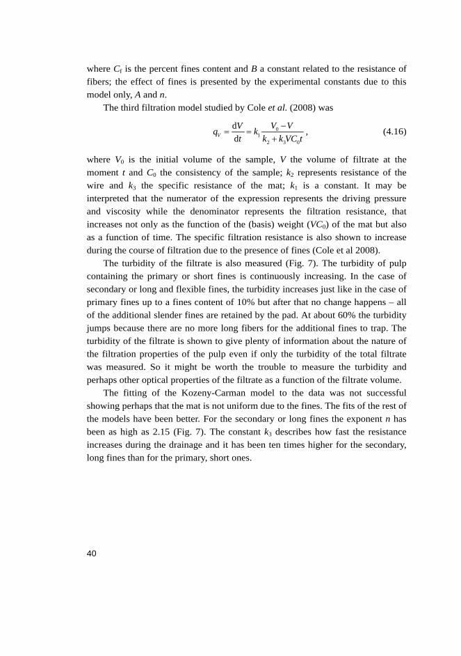
where V0 is the initial volume of the sample, V the volume of filtrate at the moment t and C0 the consistency of the sample; k2 represents resistance of the wire and k3 the specific resistance of the mat; k1 is a constant. It may be interpreted that the numerator of the expression represents the driving pressure and viscosity while the denominator represents the filtration resistance, that increases not only as the function of the (basis) weight (VC0) of the mat but also as a function of time. The specific filtration resistance is also shown to increase during the course of filtration due to the presence of fines (Cole et al 2008).
The turbidity of the filtrate is also measured (Fig. 7). The turbidity of pulp containing the primary or short fines is continuously increasing. In the case of secondary or long and flexible fines, the turbidity increases just like in the case of primary fines up to a fines content of 10% but after that no change happens – all of the additional slender fines are retained by the pad. At about 60% the turbidity jumps because there are no more long fibers for the additional fines to trap. The turbidity of the filtrate is shown to give plenty of information about the nature of the filtration properties of the pulp even if only the turbidity of the total filtrate was measured. So it might be worth the trouble to measure the turbidity and perhaps other optical properties of the filtrate as a function of the filtrate volume.
The fitting of the Kozeny-Carman model to the data was not successful showing perhaps that the mat is not uniform due to the fines. The fits of the rest of the models have been better. For the secondary or long fines the exponent n has been as high as 2.15 (Fig. 7). The constant k3 describes how fast the resistance increases during the drainage and it has been ten times higher for the secondary, long fines than for the primary, short ones.

41
Fig. 7. Effect of fines on filtration time (left) and turbidity of filtrate. The “primary fines”
are short and thick, “secondary ones” long and thin. NTU means Nephelometric
Turbidity Units (Cole et al. 2008, published by permission of TAPPI).
Many researchers have noticed that the Kozeny-Carman form of Darcy’s law is not always valid. One reason might be at least during high filtration velocities that the flow is not laminar but partly turbulent and in addition to the frictional resistance an inertia resistance is remarkable. In this case a resistance term proportional to the second power of volume flow rate per area (qA = qV /A) must be added to the frictional resistance and the pressure drop (Δp) in the mat is (Wildfong et al. 2000a):
2A A
p aq bqL
, (4.17)
where L is the height of the mat. The parameters a and b are frictional or viscous and inertial resistance coefficients, respectively. A drainage analyzer (very alike to the PDAX of this thesis) with underpressure below the screen was used to measure filtration resistances of very fast drainages. The inertia resistance was therefore supposed to dominate at least in the beginning of the filtration. The fit of experimental drainage results to the model above have given small negative values to b. So no inertia resistance was detected. The viscous resistance coefficient increased with the increase of basis weight – the steeper the higher was the fines content of the sample. Unfortunately no pulps of decreasing resistance coefficient were analyzed.
Fines Content (%) Fines Content (%)Fines Content (%) Fines Content (%)

42
Fig. 8. Effect of fines content (%, upper graph) and filtrating pressure (kPa, lower
graph) on the progression of the specific filtration resistance (Wildfong et al. 2000b,
published by permission of PAPTAC).
It was supposed by Wildfong et al. (2000b) that the increase of viscous coefficient of resistance was affected by the fines and it was studied in more detail. The increase of fines made the increase and final value of the viscous coefficient higher. When the driving pressure was increased, the retention of fines and value of a decreased. The results were interpreted so that fines plugged pores of the mat and it was more dominating than the compression of the mat due to higher pressure. Fines contents of 0% to 36% were used, the range of the basis weight was 20 g/m2 – 50 g/m2 and driving pressures were 1.7; 3.5 and 5.1 kPa. The change of the resistance coefficient during the drainage is shown graphically (Fig. 8) but its mathematical equation is not presented – except for the most common
0 %
15 %
19 %
32 %
36 %
0
2
4
6
8
10
12
14
16
18
20
15 25 35 45 55
basis weight, g/m2
a, 1
06 g
/(cm
3 s)
1,7 kPa3,5 kPa
5,1 kPa
0
1
2
3
4
5
6
7
8
9
10
15 25 35 45 55
basis weight, g/m2
a, 1
06 g
/(cm
3 s)
0 %
15 %
19 %
32 %
36 %
0
2
4
6
8
10
12
14
16
18
20
15 25 35 45 55
basis weight, g/m2
a, 1
06 g
/(cm
3 s)
1,7 kPa3,5 kPa
5,1 kPa
0
1
2
3
4
5
6
7
8
9
10
15 25 35 45 55
basis weight, g/m2
a, 1
06 g
/(cm
3 s)

43
expression: Δp/L = a(t)qA, where Δp is pressure drop over the mat, L the mat thickness, qA the filtration flow rate per area or the supervicial drainage velocity and a(t) the viscous resistance coefficient as a funtion of time.
Wildfong et al. (2001a, 2001b) has also modeled a roll forming in a pilot paper machine. Both the viscous (a0) and inertial (b0) resistance coefficients of the forming fabric have been determined for the equation Δp = a0qA + b0qA
2. Now also the inertial resistance coefficient has been significant, b0 = 95 g/cm3 when compared to viscous resistance of the wire a0 = 625 g/(cm2s) but small beside the viscous resistance of the mat. So the inertial resistance has been neglected to simplify the model. Even if Wildfong et al. (2000b) has pointed out in the former report how important it is to account for the change of the resistance during the course of drainage, the derived model is darcy-like.
The drainage of real and pilot paper machines are widely modeled, but they are outside of the scope of this thesis and would demand exhaustive descriptions of the processes. The model of roll forming by Wildfong et al. (2001a, 2001b) is however presented as an example. In roll forming, the pressure (Δp = TW/LR) is generated between the two wires by their tension (TW, N/m) and the filtrating pressure is the difference between it and the atmospheric pressure (pa) outside of the wires. The slurry is filtrated on both of the wires. The lower wire travels on the surface of a roll at the speed u. The length of the connection is Lc, its area A and the radius of the roll LR. If the viscous resistance of the wire is a0 and that of the mat a and the consistencies of slurry, mat and filtrate CHB, CM and CWW, respectively, the volume flow rate (dV/dt) through the wire may be expressed:
Wa
W2 a
0 C HB WW 00
M
1 dd
2
RA
R
T pLVq
A t T pLa L C C aa a
a a u C a
. (4.18)
The values of consistencies might be an interesting measurement problem in a real paper machine but also when realizing an analyzer to simulate this model.
Wahlström and O’Blenes (1962) have developed an empirical expression to describe the filtration process based on direct measurements using an analyzer of their own. The measurements are made after the “constant drainage conditions” or the pressure and the retention equilibrium are obtained above the basis weights of about 30 g/m2 to 70 g/m2. In the beginning of the drainage the pressure caused by

44
the accelerative force and the pressure drop across the wire are dominating but after the basis weight of about 15 g/m2 their effect is negligible. Retention equilibrium in mat formation is reached when from each layer depositing the same quantity of each fiber size is retained within the mat’s structure. In practice the constant drainage conditions are supposed to prevail when the plot time vs. logarithm of basis weight is a straight line. The consistencies of the slurry have been about 0.2% to 0.8%, filtrating pressures from about 5 kPa to 30 kPa and basis weights between 30 g/m2 and 180 g/m2. The SR-values of chemical pulps were 13.5 – 69 but only one sample of mechanical pulp was tested and its SR-value was as low as 46. Needs arise to also examine mechanical pulps of slower filtration as well as higher pressures. After the thorough sets of experiments between the quantities, the following expression was obtained to calculate the time (t) needed to filtrate a slurry the consistency of which is C0 to a mat of certain basis weight (W) using constant filtration pressure difference (Δp):
0
nGt p WC
. (4.19)
The constant G is called the drainage constant and it is said to describe the mat formed. The parameter n describes the compressibility of the mat. It depends on pulp type but not on consistency or degree of beating. The parameter α is shown to be practically independent of the pressure and consistency but a function of pulp type and beating alone. The most important observation is that α only occasionally equals to 2 suggested by Darcy’s law. The values of α were between 1.85 and 2.86. So, specific resistance has usually decreased during the course of drainage.
The equation is linearized by logarithm transformation and fitted to the measurements in order to get the parameters. This can be done if the real (and measured) filtration curve starts from the origin and the model is valid in the beginning. It was however good reason to suppose that the model is valid only in the range of the “constant filtration conditions”, not in the beginning of the drainage. So one cannot force the model curve to start from the origin. That is why the model of this thesis (Ve =kt+V0
e) includes the term V0e; its effect might
be very significant because the phenomena are so fast in the beginning. The calculation of basis weight (W) is complicated and includes many
elements of uncertainty. It is a function of drop of the level of the slurry, retention and the water fiber ratio of the mat. Many analyses must have been made using different amounts of sample and the mat formed must have been weighted to get

45
the retention curve. The height of the mat must have been measured during the drive using a transparent sample container – the limit between the mat and slurry is all but clear. In this thesis the basic equation is based on reliable direct measurements but the calculation of basis weight is rather too simplified than complicated (Chapter 7).
4.4 Models of freeness testers
El-Hosseyni & Yan (1980) has derived models of Canadian Standard Freeness analyzer by applying Darcy’s law:
dd AW
V A pt WR , (4.20)
where
V filtrated volume of liquid t time A area of the screen Δp filtrating pressure η viscosity of the flowing liquid W grammage of the mat RAWη specific filtration resistance
It is assumed that the retention is complete and the amount of solids retained in the mat per filtrated volume equals the consistency (C0) of the slurry to be filtrated:
0C VWA
. (4.21)
The pulp is filtrated using the hydrostatic pressure of the sample only, which can be calculated because the initial value of sample volume (V0) is defined and the acceleration of free fall (g) and density of fluid (ρ) are also known:
0V Vp gA
. (4.22)
By substituting Eqs. (4.21) and (4.22) to Eq. (4.20):
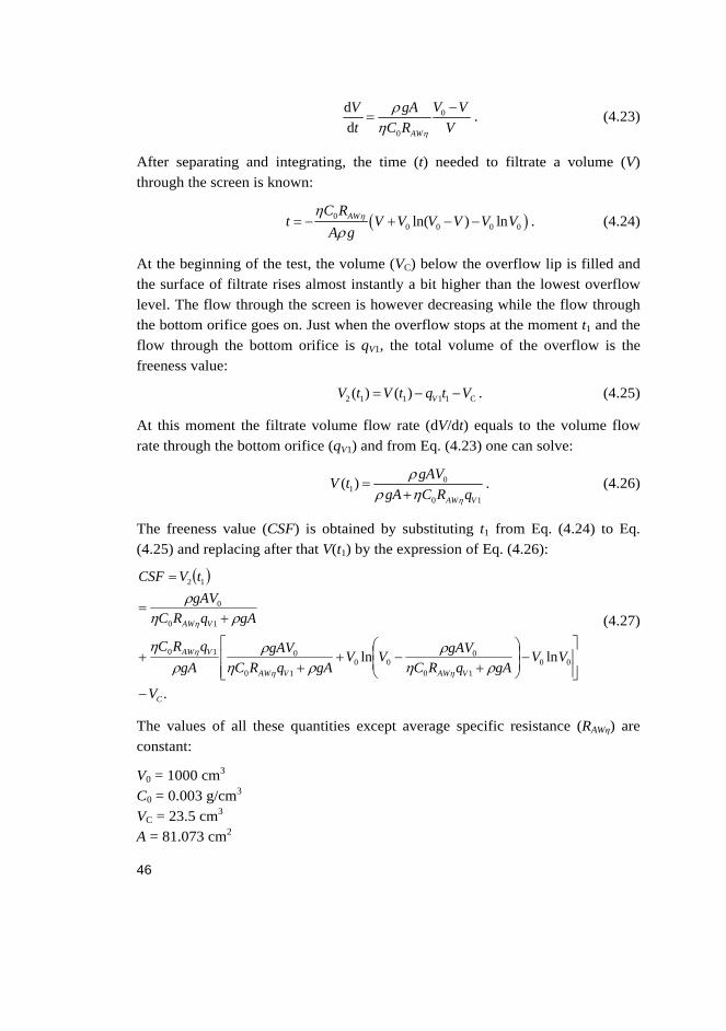
46
0
0
dd AW
V VV gAt C R V
. (4.23)
After separating and integrating, the time (t) needed to filtrate a volume (V) through the screen is known:
00 0 0 0ln( ) lnAWC R
t V V V V V VA g
. (4.24)
At the beginning of the test, the volume (VC) below the overflow lip is filled and the surface of filtrate rises almost instantly a bit higher than the lowest overflow level. The flow through the screen is however decreasing while the flow through the bottom orifice goes on. Just when the overflow stops at the moment t1 and the flow through the bottom orifice is qV1, the total volume of the overflow is the freeness value:
2 1 1 1 1 C( ) ( ) VV t V t q t V . (4.25)
At this moment the filtrate volume flow rate (dV/dt) equals to the volume flow rate through the bottom orifice (qV1) and from Eq. (4.23) one can solve:
01
0 1
( )AW V
gAVV tgA C R q
. (4.26)
The freeness value (CSF) is obtained by substituting t1 from Eq. (4.24) to Eq. (4.25) and replacing after that V(t1) by the expression of Eq. (4.26):
.
lnln 0010
000
10
010
10
0
12
C
VAWVAW
VAW
VAW
V
VVgAqRC
gAVVVgAqRC
gAVgA
qRC
gAqRCgAVtVCSF
(4.27)
The values of all these quantities except average specific resistance (RAWη) are constant:
V0 = 1000 cm3 C0 = 0.003 g/cm3 VC = 23.5 cm3 A = 81.073 cm2

47
ρ = 1.0 g/cm2 g = 9.81 m/s2 η = 0.01 g/(cm s) qV1 = 8.833 cm3/s.
So the average specific resistance can be calculated after the CSF value is measured by the tester. If the logarithm of CSF is plotted vs. the square root of RAWη a straight line is obtained (Fig.9). The specific resistance may be replaced by the Kozeny-Carman expression (e.g. RAWη = 5.55Sm
2Cm/(1 − νsCm)3) and examine how CSF is affected by the physical properties of pulp (e.g. specific surface (Sm), specific volume of solids (νs) or pad consistency (Cm)).
Fig. 9. Relation between logarithm of Canadian Standard Freeness (lg(CSF)) and the
square root of pulp average specific filtration resistance (RAWη) and CSF as a funtion
of RAWη. (El-Hosseyni & Yan 1980, published by permission of PAPTAC).
A bit less complicated formula for CSF has been derived by Swodzinsky & Doshi (1986):
lg(CSF )
CSF
2
2,1
2,2
2,3
2,4
2,5
2,6
2,7
2,8
2,9
0,5 1 1,5 2 2,5 3 3,5
lg(C
SF
)
100
200
300
400
500
600
700
0 2 4 6 8 10 12
CS
F,
ml
RAWη1/2, (109 m/kg)1/2
RAWη, 109 m/kg
lg(CSF )
CSF
2
2,1
2,2
2,3
2,4
2,5
2,6
2,7
2,8
2,9
0,5 1 1,5 2 2,5 3 3,5
lg(C
SF
)
100
200
300
400
500
600
700
0 2 4 6 8 10 12
CS
F,
ml
RAWη1/2, (109 m/kg)1/2
RAWη, 109 m/kg

48
00 C ln 1VCSF V V Y
Y
, (4.28)
where
1 0 0V AWq V C RY
gA
.
The model was developed using Darcy’s law and tested for kraft pulps only. The results have shown that the average specific filtration resistance of a pulp type is constant or Darcy’s law applies, when the consistency of the sample is greater than 0.2% and the freeness not “very high”, not more than 600 ml. The result concerning the consistency is opposite to that of Wahlström & O’Blenes (1962), but they used also mechanical pulps.

49
5 Experimental arrangements
Two measurement systems for pulp drainage analysis (say PDAX and PDAY) were built during this work. Both of them were based on a commercial (Kajaani PDA) drainage analyzer. The used analyzers were quite different from each other as well as from the original PDA. Only minor changes were however made to the former, screen – that is what the core of the main phenomenon is: filtration which is timeless even if the technology around it has been and will be developed.
The screen of PDAX on which the fiber mat was formed and through which the liquid was filtrated, was a circular grid of perpendicular metal wires. The diameter of the parallel wires in one direction was 0.3 mm and the pitch was 0.7 mm. Those of the opposite wires were 0.25 and 0.45 mm. The area of the screen was 9677 mm2 and the diameter 111 mm accordingly. The screen was on the bottom of 18 mm high (truncated) cone, the upper area of which and the upper part of the sample vessel was 11310 mm2 and the diameter 120 mm. The wire cone was connected to the scales (Fig. 10) but that was not used in this work.
In PDAX a sample conditioning system was added above the screen vessel. The sample was manually poured into the conditioning container. There it was circulated through a consistency transmitter (LC 100) based on polarized light. Temperature of the slurry was also measured (PT 100) continuously. Cold or warm water was led into the conditioning chamber constantly keeping the temperature below the set point. After reaching the consistency target the water flow was stopped but the circulation continued in order to warm the sample to the temperature target. The circulating pump and consistency meter were used as heaters. The overflow kept the volume of the sample constant. The slurry was also mixed by air bubbles conveyed into the bottom of the conditioning vessel.
The conditioned slurry was dropped through a valve into the open screen chamber.
Underpressure was connected into the suction chamber below the screen from an air container of 75 dm3. The amount of filtrate was measured in the suction chamber using an illuminating tube charged by direct voltage and a CCD camera. The light source and the camera were located on the opposite sides of the measurement glass tube that was connected by the side of the suction chamber.
The measurement sequence of PDAX was totally automated after pouring the sample into the conditioner and clicking the start button on the screen of the PC computer.
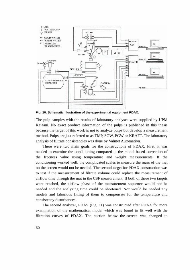
50
Fig. 10. Schematic illustration of the experimental equipment PDAX.
The pulp samples with the results of laboratory analyses were supplied by UPM Kajaani. No exact product information of the pulps is published in this thesis because the target of this work is not to analyze pulps but develop a measurement method. Pulps are just referred to as TMP, SGW, PGW or KRAFT. The laboratory analysis of filtrate consistencies was done by Valmet Automation.
There were two main goals for the constructions of PDAX. First, it was needed to examine the conditioning compared to the model based correction of the freeness value using temperature and weight measurements. If the conditioning worked well, the complicated scales to measure the mass of the mat on the screen would not be needed. The second target for PDAX construction was to test if the measurement of filtrate volume could replace the measurement of airflow time through the mat in the CSF measurement. If both of these two targets were reached, the airflow phase of the measurement sequence would not be needed and the analyzing time could be shortened. Nor would be needed any models and laborious fitting of them to compensate for the temperature and consistency disturbances.
The second analyzer, PDAY (Fig. 11) was constructed after PDAX for more examination of the mathematical model which was found to fit well with the filtration curves of PDAX. The suction below the screen was changed to

51
overpressure above the sample to prevent the influence of air bubbles on the model. Those may appear in the pulp mat or screen when the absolute pressure of water is suddenly decreased to 80 kPa. Another important question is the effect of the changes of the fines retention on the shape of the filtration curve. So an optical consistency meter (Kajaani LC 100) was fixed (to – let’s say – LCF) and installed to measure the filtrate continuously during the drainage. The filtration rate was measured by an ultrasonic distance transmitter installed on the deck of the screen chamber. The drainage cone below the screen and the pipe through LCF was full of water up to the upper level of the screen. The screen was a hole plate alike to that of the CSF tester. The diameter of it and the screen chamber were 102 mm and the area accordingly 8171 mm2.
Fig. 11. Schematic illustration of the experimental equipment PDAY.
Instead of automatic (like in PDAX) conditioning it was done manually when using PDAY. The sample was poured into the screen chamber and its deck was closed manually. After the start button was pushed the rest of the measurement sequence was controlled by a computer. The height difference from the surface of the overflow vessel to the initial surface of the sample was 500 mm. The volume of filtrate between the screen and LCF was 100 cm3.
PT LT
LCY
PRESSURECHAMBER SCREEN
OVERFLOW
PT LT
LCY
PRESSURECHAMBER SCREEN
OVERFLOW
PDFLCF
PT LT
LCY
PRESSURECHAMBER SCREEN
OVERFLOW
PT LT
LCY
PRESSURECHAMBER SCREEN
OVERFLOW
PT LT
LCY
PRESSURECHAMBER SCREEN
OVERFLOW
PT LT
LCY
PRESSURECHAMBER SCREEN
OVERFLOW
PDFLCF

52
The initial pressures of the air container were automatically controlled to 0 (PDAY only), 20, 50 (PDAY only) or 80 kPa whenever not drained. The controlling time was long enough to let the temperature of the air become constant after the suction in PDAX or the compression in PDAY. The control of the pressure is finished before the pressure of air chamber is switched to drain the sample. Immediately after that the pressure starts to change - the steeper the pressure changes the faster the filtration of the pulp is. So this internal feedback dampens the response in the filtration flow rate. It also dampens the disturbances of the flow rate by changing the pressure. If the output of the measurement system is the resistance, the interaction is more complicated because the resistance is proportional to the quotient of the pressure and the volume flow rate. Even if the pressure is constantly the driving force of the drainage, it depends on the drainability of the pulp and could be a measure of it. The only independent excitation of the system is the initial pressure of the chamber.
The fast change of air volume in the beginning of filtration also changes immediately the temperature of the air chamber. During the course of drainage the temperature returns closer to the initial value of the container, that is the temperature of the surrounding air. This change from a more adiabatic to a more isothermal process makes the driving pressure more constant after the very beginning of the filtration. Of course the adiabatic nature of the process also amplifies the fast disturbances of flow rate that may happen especially in the beginning of the drainage.
The target of this work was not to improve the basic construction or operation of the used drainage analyzer to achieve for instance the best possible repeatability of the basic filtration curves – but to model those curves to determine how crude the (mechanical) construction may be. The qualifications of the system have been optimized by commercial pressures and application needs over the course of many years. Into this very sort of analyzer the model of this work should be embedded. The same precision level was used when making the subsystems added for this research work, the filtrate volume and consistency measurements and the sample controller. The used sampling interval of basic measurements was purposefully limited to about 0.5 seconds and so was the needed data processing capacity to the level easily achieved by the microcontroller of the used drainage analyzer. The results of this research should be achieved within these technical limitations. The filtration curves produced by this robust system should be modeled no matter if the differences between the curves are caused by the differences of the measured pulps or disturbances caused

53
by the measurement system. On the other hand, no disturbances were produced on purpose either.
The very beginning of filtration was not used in modeling but the model was made in the “stabilized” part of the drainage for three main reasons. Firstly in this early phase the changes of the quantities are too fast and noisy to measure and probably too complicated and different to model using the same (hopefully) simple mathematical formula as in the stabilized phase. Secondly the resistance and condition of the wire is too dominating in the early state of filtration. And thirdly the retention is poor in the beginning but soon turns to be 100%. So the modeling was rejected inside the stable phase of slow changes and low noise, complete retention and minimal wire effect.
The pulp types were limited to those available and routinely analyzed in the Kajaani paper mill: SGW, PGW, TMP and chemical pulp (“kraft”) – still good enough a selection covering a CSF range from 30 ml to 635 ml. The maximum pressure level (80 kPa) was due to the strength of the air container of the Kajaani PDA drainage analyzer.
The “basic” pulp type in these examinations was TMP on the CSF level 100 ml and the basic driving pressure was 20 kPa. The main determining factor of dewaterability in this thesis is the amount of filtrate as a function of time (the “filtration curve”). As earlier mentioned the driving pressure is also dependent on the dewatering speed and used as a (partial) measure of drainability: when measured after a certain filtration time and naturally when the filtration resistance is calculated. The optical scattering (turbidity) and activity might be important drainability factors but in this work they are measured mainly to indicate the retention changes in the beginning of the drainage but also to preliminarily explore the possibilities of quantitative optical filtrate measurements to obtain additional quantitative information about drainability.
A typical set of basic measured curves is presented in Fig. 12. An analysis is started by switching the driving pressure (P) on. The pressure is slowly decreasing while the amount of filtrate (V) is increasing and that of the sample decreasing. After the sample is totally filtrated and the level of measurement remains even, the air starts to flow through the mat and the pressure decreases faster. The reference signal of the consistency meter (LCFR) indicates the total amount of fines in the filtrate: the inverse is proportional to the fines content or turbidity. The polarized signal (LCFM) increases with an increasing amount of optically active fines (or fiber-based material) but decreases by the increasing scattering caused by all the fines. The relation LCFM/LCFR is proportional to the

54
consistency if the proportion of fibers and total amount of solids is constant, in which one cannot however trust in this case, because the calibration seemed to change during the filtration (Chapter 11). In the very beginning the LCFM decreases and LCFR increases very fast indicating that both the fibers and total amount of fines decrease close to zero in a couple of seconds. All the solids are retained in the mat or the retention is complete after that.
The jump at about 60 s is caused by the air which fills the tube after the filtrate.
Fig. 12. An example of basic measurement curves generated by one PDAY analysis.
V
LCFM
LCFR
P
0
0,2
0,4
0,6
0,8
1
1,2
0 20 40 60 80
TIME, s
UN
SC
AL
ED_
_

55
6 The sample conditioner
The fluctuations of sample temperature and consistency are the worst disturbances of drainage analyses (Brewster & Rogers 1985). That is why the standard of laboratory analysis includes correction tables just for these two quantities (TAPPI 2004). Automatic on-line drainage meters often use experimental mathematical models to correct the error caused by the changes of temperature and consistency (Olsson 2001). Models are laborious and dependent on the measurement point in the process as well as the conditions in it. Automatic sample conditioning systems are also included in modern drainage analyzers (Kajaani, Lorentzen & Wettre, Mutek).
Possibilities and limitations to simultaneously control the temperature, consistency and volume of a sample for drainability analyses were studied. The problem of controlling these three quantities was examined and illustrated mathematically and by planning, installing and testing a simplified conditioner.
6.1 Construction and working principle of the conditioner
The volume of the conditioner was about 1.5 dm3 (Fig. 13). The amount of the sample can be set between 0.8 and 1.2 dm3 by adjusting the height of the overflow tube that was used (in addition to the easiness to set the height target of the sample level) to eliminate the effect of the surface waving on the volume of the sample. The circulation of pulp and separate, big (to avoid air dissolution) air bubbles were used to mix the slurry.
The original pulp sample was manually dropped into the container. The amount of the sample must be more than 0.5 dm3 and the consistency between 0.3 and 1.5%. The controlling computer program was started manually to control the next steps. The temperature was measured using a Pt-100 resistive temperature sensor. The pulp was pumped through the optical consistency transmitter. If the measured consistency was higher than the target, water was fed into the chamber by opening an on/off valve. The cold water valve was open (and the warm one closed) until the lower temperature level was reached (Fig. 19). It was set, e.g. to 0.3 ˚C below the final target. After that warm water was allowed to flow until the upper limit, which was e.g. 0.1 ˚C below the final target, was reached. After that the flow was switched back to cold water, and so on. The water flow was switched off when the consistency was at its set point.

56
Fig. 13. The construction principle of the sample conditioner.
6.2 Theoretical progress of the conditioning
The aim of the following theoretical examination is to evaluate the possibilities and limitations of this kind of control system. The intermediate goals are to deduce expressions for the course of consistency and temperature during the conditioning process and the final target is to find the limits for the initial values of these quantities when a suitable state for drainability measurement must be reached.
It is supposed that the container is an ideal mixer, in other words the temperature and consistency are spatially constant and that the temperatures and rate of water flows are even (while on). Only the first half cycle of those described above is modeled – the rest are alike.

57
6.2.1 Conditioning of consistency
If the mass of the initial sample (m0) is smaller than the needed amount (mt), the growth phase starts the conditioning and the mass flow rate of water (qm) lasts till
t 01 t 0, if
m
m mt m mq
(6.1)
otherwise 1 0t . The consistency (C) at the moment t can be calculated if the original
consistency (C0) is known using the fact that the amount of solids is all the time the same as in the beginning of the growth phase:
0 0 0mC m q t C m , when 10 t t (6.2)
0 0
0 m
C mCm q t
, when 10 t t . (6.3)
The consistency at the end of the growth phase and in the beginning of the overflow phase is:
0 01
t
C mCm
. (6.4)
After that the constant volume phase follows and during a differential time period (dt) the consistency all over the container and in the overflow as well is C = mk/mt and the change of mass of solid material in the container (mk) is:
kk
t
d d dm mmm q C t q tm
. (6.5)
From this equation the consistency at the moment t can be solved (Appendix 1):
11
t tC C e , when 1t t , (6.6)
where τ = mt/qm. So the conditioning time is:
11 ln Ct t
C . (6.7)
These equations can be easily (according to the targets of this work) used to evaluate the performance of a consistency conditioning.
A couple of examples concerning the course of the consistency are presented in Fig. 14.
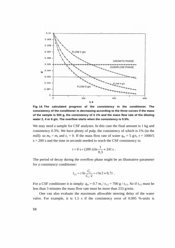
58
Fig. 14. The calculated progress of the consistency in the conditioner. The
consistency of the conditioner is decreasing according to the three curves if the mass
of the sample is 500 g, the consistency of it 1% and the mass flow rate of the diluting
water 2, 4 or 6 g/s. The overflow starts when the consistency is 0.5%.
We may need a sample for CSF analyses. In this case the final amount is 1 kg and consistency 0.3%. We have plenty of pulp, the consistency of which is 1% (in the mill): so m0 > mt and t1 = 0. If the mass flow rate of water qm = 5 g/s, τ = 1000/5 s = 200 s and the time in seconds needed to reach the CSF consistency is:
10 s (200 s) ln 241 s0,3
t .
The period of decay during the overflow phase might be an illustrative parameter for a consistency conditioner:
11 2
1
ln ln 2 0,72
CtC
.
For a CSF conditioner it is simply: qm = 0.7 mt / t1/2 = 700 g / t1/2. So if t1/2 must be less than 3 minutes the mass flow rate must be more than 233 g/min.
One can also evaluate the maximum allowable steering delay of the water valve. For example, it is 1.5 s if the consistency error of 0.005 %-units is
C
t, s
GROWTH PHASE
OVERFLOW PHASE
FLOW 2 g/s
FLOW 4 g/s
FLOW 6 g/s
C
t, s
GROWTH PHASE
OVERFLOW PHASE
FLOW 2 g/s
FLOW 4 g/s
FLOW 6 g/s

59
acceptable; or if the delay is known to be 1.5 s the water must be switched off 0.005%-units before the final target.
6.2.2 Conditioning of temperature
In addition to the previous it is assumed that the sample is heated by a constant power P due to the pump, consistency transmitter, air bubbles and conduction from or the surrounding.
The following mathematical formulas are deduced for decreasing temperature but can easily be applied also for an increasing case.
In the growth phase the mass of the sample is increasing from the initial value m0 to m during the time period from 0 to t while the temperature of the cooling or diluting water is increasing from TV to T. All the energy from the decreasing temperature of the original sample and from the heating power is bound by the heating of the cooling water. The specific heat capacity of both water and sample is supposed to be ch.
h 0 V h 0 0c m m T T c m T T Pt , (6.8)
when 0 tm m m . After substituting m = qmt the temperature at the moment t can be solved:
0
V 0 V0 h 0m m
m PtT T T Tm q t c m q t
. (6.9)
The final temperature of the growth phase (T1) is obtained by substituting t from Eq. (6.1):
0 01 V 0 V
t h
1m t
m mPT T T Tm c q m
. (6.10)
During the constant volume or overflow phase the energy balance must be calculated over a short period dt. During this time the water running into the container is qmdt and its temperature changes from TV to the sample temperature of the moment (T) while the water takes the energy from the heating power P and from the temperature change of the sample (dT):
V h h td d dmT T c q t P t c m T . (6.11)

60
This differential equation can be solved by separating the variables and integrating (Appendix 2) to get the temperature at the moment t:
1e1e
t tT T T , (6.12)
where
Vh m
PT Tc q
0e1 0 V
t h m
m PT T Tm c q
t 01
m
m mtq
t
m
mq
.
A couple of cooling curves are presented in Fig. 15.
Fig. 15. The theoretical progress of temperature in the conditioner. Y shows the start
of the overflow. The figures below the text WATER are the mass flow rate and
temperature of the cooling and diluting water.
T,
˚C
t, s
T,
˚C
t, s
WATER
4 g/s, 15 ˚C
4 g/s, 10 ˚C
6 g/s, 10 ˚C
T,
˚C
t, s
T,
˚C
t, s
WATER
4 g/s, 15 ˚C
4 g/s, 10 ˚C
6 g/s, 10 ˚C

61
6.2.3 Theoretical temperature and consistency limits for the conditioned sample
The connection between the initial temperature and consistency can be calculated by setting the times of dilution and cooling to equal values and solving the initial temperature as a function of the initial consistency:
00 t V V
t h hm m
C P PT T T TC c q c q
, (6.13)
where Ct and Tt are the consistency and temperature target, respectively. The limits of the possible initial values are linear (Fig. 16). The temperature – consistency pair should be located below the selected line. E.g., if the temperature of water is 10 ˚C and the warming power is 0, the sample with a temperature of 50 ˚C and consistency 1.5% can be cooled and diluted to CSF conditions, but it is not possible if the temperature is 70 ˚C, because the consistency target is reached before the temperature one and the water valves must be switched off.
Fig. 16. The possible temperatures and consistencies of the samples to be
conditioned. The temperature – consistency pair of the initial sample should be
located below the selected line.
THE INITIAL CONSISTENCY
TH
E IN
ITIA
L T
EM
PE
RA
TU
RE
, oC
POSSIBLE VALUES FOR CONDITIONER TO REACH 20 oC AND 0,03 %
WATER, 0 oC 5 oC10 oC
15 oC
15 oCPOWER 15 W
20 oC
THE INITIAL CONSISTENCY
TH
E IN
ITIA
L T
EM
PE
RA
TU
RE
, oC
POSSIBLE VALUES FOR CONDITIONER TO REACH 20 oC AND 0,03 %
WATER, 0 oC 5 oC10 oC
15 oC
15 oCPOWER 15 W
20 oC
THE INITIAL CONSISTENCY
TH
E IN
ITIA
L T
EM
PE
RA
TU
RE
, oC
POSSIBLE VALUES FOR CONDITIONER TO REACH 20 oC AND 0,03 %
WATER, 0 oC 5 oC10 oC
15 oC
15 oCPOWER 15 W
20 oC
THE INITIAL CONSISTENCY
TH
E IN
ITIA
L T
EM
PE
RA
TU
RE
, oC
POSSIBLE VALUES FOR CONDITIONER TO REACH 20 oC AND 0,03 %
WATER, 0 oC 5 oC10 oC
15 oC
15 oCPOWER 15 W
20 oC

62
6.3 Conditioning experiments
The consistency is controlled using an optical consistency transmitter that is based on polarized light and the optical activity of fibers (Appendix 3). The transmitter was calibrated for TMP the CSF value of which was 100 ml (Fig. 17.).
Fig. 17. The calibration of the consistency transmitter.
A typical example of consistency conditioning is presented in Fig. 18. The initial consistency was 0.75%. The target was reached in 3 minutes and the water flow was switched off. The measured consistency has settled down between 0.29% and 0.30% during the warming (Fig. 19.).
The standard deviation of the final consistency measured by the transmitter in 21 conditionings has been 0.0015%-units. It corresponds to the CSF error of 0.5 ml or 0.5% on the CSF level of 100 ml according to the correction table of the CSF standard.
The final consistency of the sample was analyzed in the laboratory after 15 conditionings. Nine times the result was 0.30% and six times 0.31%. So the consistency conditioning has been as exact as the reference analyses.
Three different set points were needed for the temperature conditioning (Fig. 19). The two lowest ones were the lower and higher limit for the control by water flow and the highest one is the final target.
0
0,1
0,2
0,3
0,4
0,5
0,6
0,7
0,8
0,9
1
0 1 2 3 4 5 6 7
LC 100 M/R , V
C,%
MEAS
CALIBR
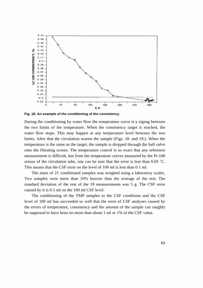
63
Fig. 18. An example of the conditioning of the consistency.
During the conditioning by water flow the temperature curve is a zigzag between the two limits of the temperature. When the consistency target is reached, the water flow stops. This may happen at any temperature level between the two limits. After that the circulation warms the sample (Figs. 18. and 19.). When the temperature is the same as the target, the sample is dropped through the ball valve onto the filtrating screen. The temperature control is so exact that any reference measurement is difficult, but from the temperature curves measured by the Pt-100 sensor of the circulation tube, one can be sure that the error is less than 0.05 ˚C. This means that the CSF error on the level of 100 ml is less than 0.1 ml.
The mass of 21 conditioned samples was weighed using a laboratory scales. Two samples were more than 10% heavier than the average of the rest. The standard deviation of the rest of the 19 measurements was 5 g. The CSF error caused by it is 0.5 ml on the 100 ml CSF level.
The conditioning of the TMP samples to the CSF conditions and the CSF level of 100 ml has succeeded so well that the error of CSF analyses caused by the errors of temperature, consistency and the amount of the sample can raughly be supposed to have been no more than about 1 ml or 1% of the CSF value.
t, s
LC 1
00
CO
NS
ISTE
NC
Y, %
THE EXPEREMENTAL PROGRESS OF CONSISTENCY CONDITIONING
t, s
LC 1
00
CO
NS
ISTE
NC
Y, %
THE EXPEREMENTAL PROGRESS OF CONSISTENCY CONDITIONING
t, s
LC 1
00
CO
NS
ISTE
NC
Y, %
THE EXPEREMENTAL PROGRESS OF CONSISTENCY CONDITIONING
t, s
LC 1
00
CO
NS
ISTE
NC
Y, %
THE EXPEREMENTAL PROGRESS OF CONSISTENCY CONDITIONING
t, s
LC
100
CO
NS
ISTE
NC
Y, %
t, s
LC 1
00
CO
NS
ISTE
NC
Y, %
THE EXPEREMENTAL PROGRESS OF CONSISTENCY CONDITIONING
t, s
LC 1
00
CO
NS
ISTE
NC
Y, %
THE EXPEREMENTAL PROGRESS OF CONSISTENCY CONDITIONING
t, s
LC 1
00
CO
NS
ISTE
NC
Y, %
THE EXPEREMENTAL PROGRESS OF CONSISTENCY CONDITIONING
t, s
LC 1
00
CO
NS
ISTE
NC
Y, %
THE EXPEREMENTAL PROGRESS OF CONSISTENCY CONDITIONING
t, s
LC
100
CO
NS
ISTE
NC
Y, %

64
Fig. 19. An example of the conditioning of the temperature.
THE EXPERIMENTAL PROGRESS OF TEMPERATURE CONDITIONING
TE
MP
ER
AT
UR
E, o
C
t, s
THE EXPERIMENTAL PROGRESS OF TEMPERATURE CONDITIONING
TE
MP
ER
AT
UR
E, o
C
t, s
THE EXPERIMENTAL PROGRESS OF TEMPERATURE CONDITIONING
TE
MP
ER
AT
UR
E, o
C
t, s
THE EXPERIMENTAL PROGRESS OF TEMPERATURE CONDITIONING
TE
MP
ER
AT
UR
E, o
C
t, s t, s
TE
MP
ER
AT
UR
E, ˚
C
THE EXPERIMENTAL PROGRESS OF TEMPERATURE CONDITIONING
TE
MP
ER
AT
UR
E, o
C
t, s
THE EXPERIMENTAL PROGRESS OF TEMPERATURE CONDITIONING
TE
MP
ER
AT
UR
E, o
C
t, s
THE EXPERIMENTAL PROGRESS OF TEMPERATURE CONDITIONING
TE
MP
ER
AT
UR
E, o
C
t, s
THE EXPERIMENTAL PROGRESS OF TEMPERATURE CONDITIONING
TE
MP
ER
AT
UR
E, o
C
t, s t, s
TE
MP
ER
AT
UR
E, ˚
C

65
7 Applied model
For some reason or other when using PDAX or PDAY the experimental filtration curves of mechanical pulps appeared to be more ”curvy” compared to the mathematical models deduced from Darcy’s law (V2 = kt), which on the contrary were more curvy than the experimental curves of chemical pulps (Figs. 20 and 21). A formula giving a much better fitting is needed.
After deciding to use a purely empirical “black box” model, one is not bound to deduction from physical properties of pulp when choosing the mathematical formula of the model. In special cases the experimental, measured curves are close enough to Darcy’s curves. Therefore it would be most desirable that in these cases our mathematical formula would be exactly the same as Darcy’s mathematical formula. Darcy’s formula is the very basic and most widely used formula to describe filtration. That is why it would be useful if the experimental model could be easily compared to Darcy’s law: how “darcy-like” the measured pulp is. The natural way to control the curvature of the model is to change the exponent (e) of the filtration volume (Ve = kt) or that of sample or filtrate level (L). In that case the exponent e = 2 suggested by Darcy’s law is included in our model as a special case and the difference of the exponent from 2 might be used to describe how strongly the resistancy of the pulp mat is changing during the filtration or how un-darcy-like the pulp is.
On hand, there is no natural reason why changing the exponent e from 2 would turn the model to run closer to the measured curve in general. Still, it is less sure that the model would be suitable for different types of pulps, driving pressures and drainage equipment. The suitability must be studied experimentally. Nor is there any self-evident lower limit for the fit between the model and measurements. The limit will be determined on the grounds of expediency. In this work the fit is studied for two analyzers described in Chapter 5 using a wide but however limited range of pulp types and driving pressures – well knowing that they are only some special cases and humbly admitting the generalization difficulties due to the huge variety of used filtration processes and filtrated materials in the paper making industry – still believing that the results of this work might be adapted for more general use.

66
Fig. 20. Fit of Darcy’s model V2 = kt + V02 to measured filtration curves TMP (left) and
chemical pulp (right).
Fig. 21. Fit of Darcy’s model, V2 = kt+ V02 compared to the ideal fit (“MODEL”) which
means that values of model and measurements are equal.
FIT OF "DARCY" MODEL, TMP
MEAS
0
200
400
600
800
1000
3 13 23 33 43 53
t, s
V, m
l
MEAS
MODEL
FIT OF "DARCY" MODEL, KRAFT
MEAS
MODEL
0
200
400
600
800
1000
4 5 6 7 8 9 10
t, s
V,
ml
FIT OF "DARCY" MODEL, TMP
MEAS
0
200
400
600
800
1000
3 13 23 33 43 53
t, s
V, m
l
MEAS
MODEL
FIT OF "DARCY" MODEL, KRAFT
MEAS
MODEL
0
200
400
600
800
1000
4 5 6 7 8 9 10
t, s
V,
ml
FIT OF "DARCY" MODEL, TMP
MEAS
0
200
400
600
800
1000
3 13 23 33 43 53
t, s
V, m
l
MEAS
MODEL
FIT OF "DARCY" MODEL, KRAFT
MEAS
MODEL
0
200
400
600
800
1000
4 5 6 7 8 9 10
t, s
V,
ml
FIT OF "DARCY" MODEL, TMP
MEAS
0
200
400
600
800
1000
3 13 23 33 43 53
t, s
V, m
l
MEAS
MODEL
FIT OF "DARCY" MODEL, KRAFT
MEAS
MODEL
0
200
400
600
800
1000
4 5 6 7 8 9 10
t, s
V,
ml
V,
cm3
V,
cm3
FIT OF "DARCY" MODEL, TMP
MEAS
0
200
400
600
800
1000
3 13 23 33 43 53
t, s
V, m
l
MEAS
MODEL
FIT OF "DARCY" MODEL, KRAFT
MEAS
MODEL
0
200
400
600
800
1000
4 5 6 7 8 9 10
t, s
V,
ml
FIT OF "DARCY" MODEL, TMP
MEAS
0
200
400
600
800
1000
3 13 23 33 43 53
t, s
V, m
l
MEAS
MODEL
FIT OF "DARCY" MODEL, KRAFT
MEAS
MODEL
0
200
400
600
800
1000
4 5 6 7 8 9 10
t, s
V,
ml
FIT OF "DARCY" MODEL, TMP
MEAS
0
200
400
600
800
1000
3 13 23 33 43 53
t, s
V, m
l
MEAS
MODEL
FIT OF "DARCY" MODEL, KRAFT
MEAS
MODEL
0
200
400
600
800
1000
4 5 6 7 8 9 10
t, s
V,
ml
FIT OF "DARCY" MODEL, TMP
MEAS
0
200
400
600
800
1000
3 13 23 33 43 53
t, s
V, m
l
MEAS
MODEL
FIT OF "DARCY" MODEL, KRAFT
MEAS
MODEL
0
200
400
600
800
1000
4 5 6 7 8 9 10
t, s
V,
ml
V,
cm3
V,
cm3
t, s t, s
V,
ml
V,
ml
V,
ml
FIT OF "DARCY" MODEL, TMP
MEAS
0
200
400
600
800
1000
3 13 23 33 43 53
t, s
V, m
l
MEAS
MODEL
FIT OF "DARCY" MODEL, KRAFT
MEAS
MODEL
0
200
400
600
800
1000
4 5 6 7 8 9 10
t, s
V,
ml
FIT OF "DARCY" MODEL, TMP
MEAS
0
200
400
600
800
1000
3 13 23 33 43 53
t, s
V, m
l
MEAS
MODEL
FIT OF "DARCY" MODEL, KRAFT
MEAS
MODEL
0
200
400
600
800
1000
4 5 6 7 8 9 10
t, s
V,
ml
FIT OF "DARCY" MODEL, TMP
MEAS
0
200
400
600
800
1000
3 13 23 33 43 53
t, s
V, m
l
MEAS
MODEL
FIT OF "DARCY" MODEL, KRAFT
MEAS
MODEL
0
200
400
600
800
1000
4 5 6 7 8 9 10
t, s
V,
ml
FIT OF "DARCY" MODEL, TMP
MEAS
0
200
400
600
800
1000
3 13 23 33 43 53
t, s
V, m
l
MEAS
MODEL
FIT OF "DARCY" MODEL, KRAFT
MEAS
MODEL
0
200
400
600
800
1000
4 5 6 7 8 9 10
t, s
V,
ml
V,
cm3
V,
cm3
FIT OF "DARCY" MODEL, TMP
MEAS
0
200
400
600
800
1000
3 13 23 33 43 53
t, s
V, m
l
MEAS
MODEL
FIT OF "DARCY" MODEL, KRAFT
MEAS
MODEL
0
200
400
600
800
1000
4 5 6 7 8 9 10
t, s
V,
ml
FIT OF "DARCY" MODEL, TMP
MEAS
0
200
400
600
800
1000
3 13 23 33 43 53
t, s
V, m
l
MEAS
MODEL
FIT OF "DARCY" MODEL, KRAFT
MEAS
MODEL
0
200
400
600
800
1000
4 5 6 7 8 9 10
t, s
V,
ml
FIT OF "DARCY" MODEL, TMP
MEAS
0
200
400
600
800
1000
3 13 23 33 43 53
t, s
V, m
l
MEAS
MODEL
FIT OF "DARCY" MODEL, KRAFT
MEAS
MODEL
0
200
400
600
800
1000
4 5 6 7 8 9 10
t, s
V,
ml
FIT OF "DARCY" MODEL, TMP
MEAS
0
200
400
600
800
1000
3 13 23 33 43 53
t, s
V, m
l
MEAS
MODEL
FIT OF "DARCY" MODEL, KRAFT
MEAS
MODEL
0
200
400
600
800
1000
4 5 6 7 8 9 10
t, s
V,
ml
V,
cm3
V,
cm3
t, s t, s
V,
ml
V,
ml
V,
ml
V,c
m3
V, c
m3
FIT OF "DARCY" MODEL, TMP
MEAS
0
200
400
600
800
1000
3 13 23 33 43 53
t, s
V, m
l
MEAS
MODEL
FIT OF "DARCY" MODEL, KRAFT
MEAS
MODEL
0
200
400
600
800
1000
4 5 6 7 8 9 10
t, s
V,
ml
FIT OF "DARCY" MODEL, TMP
MEAS
0
200
400
600
800
1000
3 13 23 33 43 53
t, s
V, m
l
MEAS
MODEL
FIT OF "DARCY" MODEL, KRAFT
MEAS
MODEL
0
200
400
600
800
1000
4 5 6 7 8 9 10
t, s
V,
ml
FIT OF "DARCY" MODEL, TMP
MEAS
0
200
400
600
800
1000
3 13 23 33 43 53
t, s
V, m
l
MEAS
MODEL
FIT OF "DARCY" MODEL, KRAFT
MEAS
MODEL
0
200
400
600
800
1000
4 5 6 7 8 9 10
t, s
V,
ml
FIT OF "DARCY" MODEL, TMP
MEAS
0
200
400
600
800
1000
3 13 23 33 43 53
t, s
V, m
l
MEAS
MODEL
FIT OF "DARCY" MODEL, KRAFT
MEAS
MODEL
0
200
400
600
800
1000
4 5 6 7 8 9 10
t, s
V,
ml
V,
cm3
V,
cm3
FIT OF "DARCY" MODEL, TMP
MEAS
0
200
400
600
800
1000
3 13 23 33 43 53
t, s
V, m
l
MEAS
MODEL
FIT OF "DARCY" MODEL, KRAFT
MEAS
MODEL
0
200
400
600
800
1000
4 5 6 7 8 9 10
t, s
V,
ml
FIT OF "DARCY" MODEL, TMP
MEAS
0
200
400
600
800
1000
3 13 23 33 43 53
t, s
V, m
l
MEAS
MODEL
FIT OF "DARCY" MODEL, KRAFT
MEAS
MODEL
0
200
400
600
800
1000
4 5 6 7 8 9 10
t, s
V,
ml
FIT OF "DARCY" MODEL, TMP
MEAS
0
200
400
600
800
1000
3 13 23 33 43 53
t, s
V, m
l
MEAS
MODEL
FIT OF "DARCY" MODEL, KRAFT
MEAS
MODEL
0
200
400
600
800
1000
4 5 6 7 8 9 10
t, s
V,
ml
FIT OF "DARCY" MODEL, TMP
MEAS
0
200
400
600
800
1000
3 13 23 33 43 53
t, s
V, m
l
MEAS
MODEL
FIT OF "DARCY" MODEL, KRAFT
MEAS
MODEL
0
200
400
600
800
1000
4 5 6 7 8 9 10
t, s
V,
ml
V,
cm3
V,
cm3
t, s t, s
V,
ml
V,
ml
V,
ml
FIT OF "DARCY" MODEL, TMP
MEAS
0
200
400
600
800
1000
3 13 23 33 43 53
t, s
V, m
l
MEAS
MODEL
FIT OF "DARCY" MODEL, KRAFT
MEAS
MODEL
0
200
400
600
800
1000
4 5 6 7 8 9 10
t, s
V,
ml
FIT OF "DARCY" MODEL, TMP
MEAS
0
200
400
600
800
1000
3 13 23 33 43 53
t, s
V, m
l
MEAS
MODEL
FIT OF "DARCY" MODEL, KRAFT
MEAS
MODEL
0
200
400
600
800
1000
4 5 6 7 8 9 10
t, s
V,
ml
FIT OF "DARCY" MODEL, TMP
MEAS
0
200
400
600
800
1000
3 13 23 33 43 53
t, s
V, m
l
MEAS
MODEL
FIT OF "DARCY" MODEL, KRAFT
MEAS
MODEL
0
200
400
600
800
1000
4 5 6 7 8 9 10
t, s
V,
ml
FIT OF "DARCY" MODEL, TMP
MEAS
0
200
400
600
800
1000
3 13 23 33 43 53
t, s
V, m
l
MEAS
MODEL
FIT OF "DARCY" MODEL, KRAFT
MEAS
MODEL
0
200
400
600
800
1000
4 5 6 7 8 9 10
t, s
V,
ml
V,
cm3
V,
cm3
FIT OF "DARCY" MODEL, TMP
MEAS
0
200
400
600
800
1000
3 13 23 33 43 53
t, s
V, m
l
MEAS
MODEL
FIT OF "DARCY" MODEL, KRAFT
MEAS
MODEL
0
200
400
600
800
1000
4 5 6 7 8 9 10
t, s
V,
ml
FIT OF "DARCY" MODEL, TMP
MEAS
0
200
400
600
800
1000
3 13 23 33 43 53
t, s
V, m
l
MEAS
MODEL
FIT OF "DARCY" MODEL, KRAFT
MEAS
MODEL
0
200
400
600
800
1000
4 5 6 7 8 9 10
t, s
V,
ml
FIT OF "DARCY" MODEL, TMP
MEAS
0
200
400
600
800
1000
3 13 23 33 43 53
t, s
V, m
l
MEAS
MODEL
FIT OF "DARCY" MODEL, KRAFT
MEAS
MODEL
0
200
400
600
800
1000
4 5 6 7 8 9 10
t, s
V,
ml
FIT OF "DARCY" MODEL, TMP
MEAS
0
200
400
600
800
1000
3 13 23 33 43 53
t, s
V, m
l
MEAS
MODEL
FIT OF "DARCY" MODEL, KRAFT
MEAS
MODEL
0
200
400
600
800
1000
4 5 6 7 8 9 10
t, s
V,
ml
V,
cm3
V,
cm3
t, s t, s
V,
ml
V,
ml
V,
ml
V,c
m3
V, c
m3
FIT OF "DARCY" MODEL
MODEL
KRAFT
TMP
0
200
400
600
800
1000
0 200 400 600 800 1000
V, MODEL, ml
V,
MO
DE
L A
ND
ME
AS
UR
ED
, m
l
FIT OF "DARCY" MODEL
MODEL
KRAFT
TMP
0
200
400
600
800
1000
0 200 400 600 800 1000
V, MODEL, ml
V,
MO
DE
L A
ND
ME
AS
UR
ED
, m
l
V, MODEL, cm3
V, M
OD
EL
AN
D M
EA
SU
RE
D, cm
3
FIT OF "DARCY" MODEL
MODEL
KRAFT
TMP
0
200
400
600
800
1000
0 200 400 600 800 1000
V, MODEL, ml
V,
MO
DE
L A
ND
ME
AS
UR
ED
, m
l
FIT OF "DARCY" MODEL
MODEL
KRAFT
TMP
0
200
400
600
800
1000
0 200 400 600 800 1000
V, MODEL, ml
V,
MO
DE
L A
ND
ME
AS
UR
ED
, m
l
V, MODEL, cm3
V, M
OD
EL
AN
D M
EA
SU
RE
D, cm
3
V, MODEL, ml
V, M
OD
EL
AN
D M
EA
SU
RE
D, m
l
FIT OF "DARCY" MODEL
MODEL
KRAFT
TMP
0
200
400
600
800
1000
0 200 400 600 800 1000
V, MODEL, ml
V,
MO
DE
L A
ND
ME
AS
UR
ED
, m
l
FIT OF "DARCY" MODEL
MODEL
KRAFT
TMP
0
200
400
600
800
1000
0 200 400 600 800 1000
V, MODEL, ml
V,
MO
DE
L A
ND
ME
AS
UR
ED
, m
l
V, MODEL, cm3
V, M
OD
EL
AN
D M
EA
SU
RE
D, cm
3
FIT OF "DARCY" MODEL
MODEL
KRAFT
TMP
0
200
400
600
800
1000
0 200 400 600 800 1000
V, MODEL, ml
V,
MO
DE
L A
ND
ME
AS
UR
ED
, m
l
FIT OF "DARCY" MODEL
MODEL
KRAFT
TMP
0
200
400
600
800
1000
0 200 400 600 800 1000
V, MODEL, ml
V,
MO
DE
L A
ND
ME
AS
UR
ED
, m
l
V, MODEL, cm3
V, M
OD
EL
AN
D M
EA
SU
RE
D, cm
3
V, MODEL, ml
V, M
OD
EL
AN
D M
EA
SU
RE
D, m
l
V, MODEL, cm3
V, M
OD
EL
AN
D M
EA
SU
RE
D, c
m3

67
The first few seconds of drainage are hard to measure using the selected robust technology because the phenomena and signals are fast and noisy. The shape of the filtration curve cannot be the same in the beginning as in the later phase of filtration. To overcome these difficulties the selected basic model (Ve = kt) is supplemented by one more parameter (V0
e). It does not bear any information about the quality of pulp and is used only during modeling and can be removed from the model as soon as the two meaningful parameters e and k have been determined.
The utility of the filtration model is also dependent on whether it remains simple and demonstrative enough when used to calculate the specific resistance – the most real measure of the dewaterability of the pulp itself.
In the following chapters the selected mathematical model of filtration and some deduced formulas are presented.
7.1 Model of filtration curve
The hypothetic model of the filtration curve in this work is
0e eV kt V , (7.1)
where V is the filtrated volume at the moment t, V0 that at the moment t = 0, e and k parameters, which depend on the pulp and filtration system and must be determined experimentally. V0 is also determined experimentally but does not depend on the pulp but only on the selection of the moment, when the timing of individual filtration is started. The selected mathematical formula makes it possible to freely start the timing and removing V0 without any effects on the shape of the modeled filtration curve. So V0 is just ignored in the following examination and the next simplified formula is used as the model of the filtration curve:
eV kt . (7.2)
From this one can solve the filtration volume until time t:
1 1e eV k t (7.3)
as well as the time needed to filtrate the volume V:
1 et Vk
. (7.4)

68
7.2 Filtration flow
The volume flow rate of filtrate or volumetric filtration rate (qV) as a function of time can be calculated by differentiating Eq. (7.3):
11 11
1 1
d 1d
e ee
V e
V k kq tt e e t
. (7.5)
The filtration rate can be expressed as a function of filtration volume by substituting the expression of t from Eq. (7.4) to Eq. (7.5):
11
1 eV e
k kq Ve V e
. (7.6)
Let us assume that all times during the drainage the consistency of the sample (C0) and the area of pulp mat (A) are constant and the retention into the mat is complete. Let us also assume that a great majority of solids in the mat is from the slurry filtrated through the mat (and only a small minority from the slurry displaced by the growing mat). In this case the grammage of the mat (W) as a function of time and filtrated volume is:
0CW VA
(7.7)
1 10 e eCW k tA
(7.8)
and the filtration rate can be calculated with the help of the modeled parameters also as a function of the grammage:
1
01
1e
V e
Ckqe A W
. (7.9)
7.3 Superficial velocity
The filtration rate is usually described by the volume flow rate (e.g. in cm3/s) in spite of the fact that the volume flow rate of a drainage tester depends also on the area of the screen (and the pad on it). The (average) volume flow rate is the same above the surface of the mat and inside the mat while the average velocity of the flowing material is higher (and more unclear) inside the mat than above it. The average superficial velocity (usually referred shortly as velocity) of the filtration
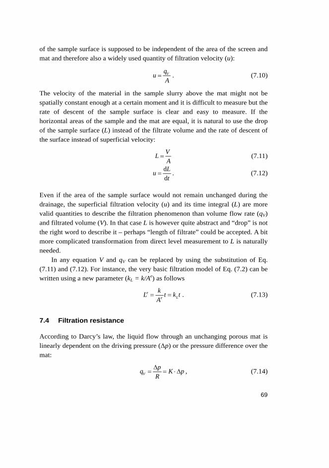
69
of the sample surface is supposed to be independent of the area of the screen and mat and therefore also a widely used quantity of filtration velocity (u):
VquA
. (7.10)
The velocity of the material in the sample slurry above the mat might not be spatially constant enough at a certain moment and it is difficult to measure but the rate of descent of the sample surface is clear and easy to measure. If the horizontal areas of the sample and the mat are equal, it is natural to use the drop of the sample surface (L) instead of the filtrate volume and the rate of descent of the surface instead of superficial velocity:
VLA
(7.11)
ddLut
. (7.12)
Even if the area of the sample surface would not remain unchanged during the drainage, the superficial filtration velocity (u) and its time integral (L) are more valid quantities to describe the filtration phenomenon than volume flow rate (qV) and filtrated volume (V). In that case L is however quite abstract and “drop” is not the right word to describe it – perhaps “length of filtrate” could be accepted. A bit more complicated transformation from direct level measurement to L is naturally needed.
In any equation V and qV can be replaced by using the substitution of Eq. (7.11) and (7.12). For instance, the very basic filtration model of Eq. (7.2) can be written using a new parameter (kL = k/Ae) as follows
eLe
kL t k tA
. (7.13)
7.4 Filtration resistance
According to Darcy’s law, the liquid flow through an unchanging porous mat is linearly dependent on the driving pressure (Δp) or the pressure difference over the mat:
Vpq K p
R
, (7.14)

70
where R is a constant property of the particular mat and liquid called resistance (of the volume flow rate – more precisely symbolized by, e.g. RV), which is independent of the driving pressure. The inverse of the resistance is called permeability (K or KV).
This total resistance (and permeability) can be separated into many kinds of specific resistances (RX) and quantities (X): R = RX X or RX = R/X. The resistance is expressed, e.g. per area of the mat (RA), in which case it can be interpreted as the resistance against the superficial velocity of the sample (u):
VA
p pqR R A
=> V
A
q puA R
.
The resistance is not dependent only on the mat but also on the properties of the flowing material – usually described by the dynamic viscosity of the fluid (η). In many dewatering analyses it is not measured or otherwise exactly known. (Who knows the complicated power consuming interactions between the fluid and many kinds of particles inside the pad!) There would have been better reasons to include it in the value of resistance but it is however usually separated from the resistance in order to scale the values of resistivity units using the viscosity of water: R = Rηη and RS = RSηη. Also in this work the viscosity of the flowing material (η) is included in the specific resistance RS and the nominal value of the viscosity of water is used as a scaling factor to make the values a bit more comparable with other research works.
If the internal structure of the mat is homogenous enough for the particular application, its resistance can be increased by increasing the height (in the direction of the flow) or the grammage (W = m/A) of the mat and decreased by increasing its area (perpendicular to the flow):
SR WRA
, (7.15)
where RS is the specific resistance of the mat – the resistance per the grammage and area of the mat. So the specific resistance is the property of the material and internal structure of the mat but independent of the size of the mat. It is however dependent on the viscosity of the flowing material if it is not separated.
The flow through the mat (Eq. 7.14) can now be calculated by

71
S S
VA Aq p p
R W R W . (7.16)
Supposing that during filtration of the pulp slurry, the grammage increases according to the Eq. (7.8) and that the flow of filtrate decreases according to our drainage model of Eq. (7.4), we can solve the specific resistance as a function of time:
2
1 2S 2
0
ee
A eR p tC k
. (7.17)
When time is picked up from Eq. (7.4) into Eq. (7.17), the specific resistance is solved as a function of filtrate volume:
2
2S
0
eA eR p VC k
. (7.18)
Perhaps the most fundamental filtration curve or equation describes the specific resistance as a function of the grammage. For getting it one must solve V from Eq. (7.7) and substitute it to Eq. (7.18):
2S 1
0
ee
e
A eR p WC k
. (7.19)
7.5 Uniform drainage
During a uniform or darcy-like drainage, the specific resistance remains even. If the driving pressure is constant and in our model the exponent e = 2, in Eqs. (7.17), (7.18) and (7.19) the exponents of t, V and W equal zero and RS is therefore independent of time, filtrated volume and grammage. The specific resistance increases during the course of drainage when e > 2 and decreases when e < 2.
When (like in our system) the pressure is decreasing, the specific resistance might be constant or increasing even if e > 2 and the trend of the specific resistance must be solved by measuring the pressure experimentally. One must also be reminded that there is no direct way to predict what the filtration curve would have been like if the pressure would have been, e.g. constant instead of the decreasing one.

72
According to Eqs. (7.17), (7.18) and (7.19) the specific resistance would be infinite in the beginning of the drainage in the case of the decreasing specific resistance and zero in the case of the increasing specific resistance. Both of the cases are unrealistic – one more reason not to start the modeling from the origin.
7.6 Logarithmic filtration curves
One of the main advantages of the model used in this study is the easiness of linearizing the equations by using any base logarithms of the quantities:
log V = (1/e)log t + ((1/e)log k) (7.20) log qV = (1/e − 1)log t + ((1/e)log k − log e) (7.21) log qV = (1 − e)log V + (log k − log e) (7.22) log qV = (1 − e)log W + (log k − log e + (e − 1)(log C0) − log A)) (7.23) log RS = (1 − 2/e)log t + (log P+2log A − log C0+log e − (2/e)log k) (7.24) log RS = (e − 2)log V + (log P+2log A − log C0+log e − log k) (7.25) log RS = (e − 2)log W + (log P+elog A − (e − 1)log C0+log e − log k). (7.26)
All of these equations describe the logarithmic quantities Y of the left side of the equations as a linear function of the logarithmic quantities X of the right side of the equations: Y = αX + ß, where α and ß are constants (if the driving pressure, Δp is constant).
7.7 Solving the parameters of the filtration curve
The parameters of the filtration model can be solved when the starting time and the filtration volumes (V1 and V2) at two different moments (t1 and t2) are known. According to Eq. (7.2): 1 1
eV kt 2 2
eV kt . From these two simple equations one can solve:
1 2
1 2
log loglog log
t teV V
(7.27)
2 1 1 2
1 2
log log log logloglog log
V t V tkV V
. (7.28)
Supposing that our model is valid (enough for some purpose) the information of any filtration curve can be stored in four numbers by measuring twice the amount
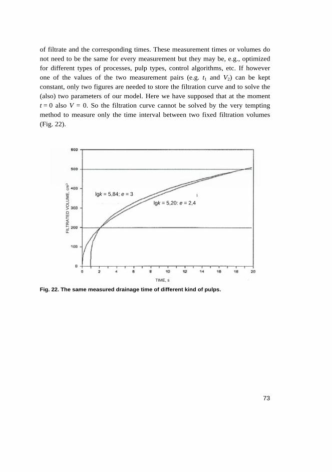
73
of filtrate and the corresponding times. These measurement times or volumes do not need to be the same for every measurement but they may be, e.g., optimized for different types of processes, pulp types, control algorithms, etc. If however one of the values of the two measurement pairs (e.g. t1 and V2) can be kept constant, only two figures are needed to store the filtration curve and to solve the (also) two parameters of our model. Here we have supposed that at the moment t = 0 also V = 0. So the filtration curve cannot be solved by the very tempting method to measure only the time interval between two fixed filtration volumes (Fig. 22).
Fig. 22. The same measured drainage time of different kind of pulps.
TIME, s
FIL
TR
AT
ED
VO
LUM
E, m
l
lgk = 5,20; e = 2,4lgk = 5,84; e = 3
TIME, s
FIL
TR
AT
ED
VO
LUM
E, m
l
lgk = 5,20; e = 2,4lgk = 5,84; e = 3
FIL
TR
AT
ED
VO
LUM
E, c
m3
TIME, s
FIL
TR
AT
ED
VO
LUM
E, m
l
lgk = 5,20; e = 2,4lgk = 5,84; e = 3
TIME, s
FIL
TR
AT
ED
VO
LUM
E, m
l
lgk = 5,20; e = 2,4lgk = 5,84; e = 3
FIL
TR
AT
ED
VO
LUM
E, c
m3
lgk = 5,20: e = 2,4
lgk = 5,84; e = 3
TIME, s
FIL
TR
AT
ED
VO
LUM
E, m
l
lgk = 5,20; e = 2,4lgk = 5,84; e = 3
TIME, s
FIL
TR
AT
ED
VO
LUM
E, m
l
lgk = 5,20; e = 2,4lgk = 5,84; e = 3
FIL
TR
AT
ED
VO
LUM
E, c
m3
TIME, s
FIL
TR
AT
ED
VO
LUM
E, m
l
lgk = 5,20; e = 2,4lgk = 5,84; e = 3
TIME, s
FIL
TR
AT
ED
VO
LUM
E, m
l
lgk = 5,20; e = 2,4lgk = 5,84; e = 3
FIL
TR
AT
ED
VO
LUM
E, c
m3
lgk = 5,20: e = 2,4
lgk = 5,84; e = 3

74

75
8 Fitting to the measurements
The method used to determine the filtration curve based on two-level measurements (Fig. 22) is possible if the model is known to be correct and measurements are not too noisy. In this work the model is empirical and rough technology and is used both in the filtrating and measuring of it. The quality of the model have been studied experimentally and one of the motives of the work is to overcome the noisy measurement surroundings. Thus lots of filtrations and measurements during each filtration are made to fit the selected model to the measurements and thereby to determine the utility of the model.
8.1 Used fitting method
We could have used the model Ve = kt and the simple regression analysis if we should be able to measure the starting point of filtration exactly. This would have been technologically very demanding because the phenomena are so fast and the signals noisy in the very beginning of filtration. We however intended to use not only a simple data processing but also rough technology. So, a bit more complicated model Ve = kt + V0
e and the following simple “home-made” algorithm were adopted to find both the two informative parameters and the origin.
The linear model Ve = kt + V0e was fitted to the measurement pairs of (t, Ve)
using the linear least squares fit to find out the parameters k and V0e. The third
parameter e was solved by calculating the regression analyses changing the values of e in the steps of 0.01 until the best correlation coefficient (or coefficient of determination) was achieved (Fig. 23). So the starting value of e (e.g. e = 1.00) was set, the measured values of Ve were calculated, the regression analysis was done to get k, V0
e and the correlation coefficient R; the value of e was incremented by 0.01 (e.g. to e = 1.01) and the analysis was repeated until the maximum of R was found.

76
Fig. 23. The determination of the model parameter e. The pressure of 20 kPa was used.
The figures next to the texts of pulp types are freeness values (ml).
The regression analysis was done starting from many different values of t or V and finishing to many different values of t or V. The main analyses were however made between 150 and 900 cm3 using PDAY. When using PDAX the main modeling was started 0.5 seconds after the filtrated volume has exceeded 222 cm3 and finished on the level of 900 cm3. The modeling was not automatically made for all the measured curves between these limits. The target was to model normal, stable dewatering. So the “normalities” of the measured curves were inspected also visually. Some analyses were totally rejected and not modeled at all, e.g. mats of the finest SGW pulps were broken by the highest pressures and there would have been no sense in modeling them. In some cases the starting or finishing point was changed. The modeling was not started from a single peak of measurement signal even if higher than the triggering level mentioned above. Most usually the upper limit was lowered because the driving pressure was not high enough to filtrate more of the sample.
The fit was made and the correlation coefficient R calculated using the linear regression analysis function of the Microsoft EXCEL PC program.
8.2 Quality of the fit of the model and the measurement
In this work the R2 values of the regression analyses of the filtration curves have been typically more than 0.999 or 99.9%. Even without any formal comparison
0,2 bar
TMP 110 mlKRAFT632 ml
0,998000,998200,998400,998600,998800,999000,999200,999400,999600,999801,00000
1,00 1,50 2,00 2,50
e
R2
0,2 bar
TMP 110 mlKRAFT632 ml
0,998000,998200,998400,998600,998800,999000,999200,999400,999600,999801,00000
1,00 1,50 2,00 2,50
e
R2
0,2 bar
TMP 110 mlKRAFT632 ml
0,998000,998200,998400,998600,998800,999000,999200,999400,999600,999801,00000
1,00 1,50 2,00 2,50
e
R2
0,2 bar
TMP 110 mlKRAFT632 ml
0,998000,998200,998400,998600,998800,999000,999200,999400,999600,999801,00000
1,00 1,50 2,00 2,50
e
R2
0,2 bar
TMP 110 mlKRAFT632 ml
0,998000,998200,998400,998600,998800,999000,999200,999400,999600,999801,00000
1,00 1,50 2,00 2,50
e
R2
0,2 bar
TMP 110 mlKRAFT632 ml
0,998000,998200,998400,998600,998800,999000,999200,999400,999600,999801,00000
1,00 1,50 2,00 2,50
e
R2
e
R2
0,2 bar
TMP 110 mlKRAFT632 ml
0,998000,998200,998400,998600,998800,999000,999200,999400,999600,999801,00000
1,00 1,50 2,00 2,50
e
R2
0,2 bar
TMP 110 mlKRAFT632 ml
0,998000,998200,998400,998600,998800,999000,999200,999400,999600,999801,00000
1,00 1,50 2,00 2,50
e
R2
0,2 bar
TMP 110 mlKRAFT632 ml
0,998000,998200,998400,998600,998800,999000,999200,999400,999600,999801,00000
1,00 1,50 2,00 2,50
e
R2
0,2 bar
TMP 110 mlKRAFT632 ml
0,998000,998200,998400,998600,998800,999000,999200,999400,999600,999801,00000
1,00 1,50 2,00 2,50
e
R2
0,2 bar
TMP 110 mlKRAFT632 ml
0,998000,998200,998400,998600,998800,999000,999200,999400,999600,999801,00000
1,00 1,50 2,00 2,50
e
R2
0,2 bar
TMP 110 mlKRAFT632 ml
0,998000,998200,998400,998600,998800,999000,999200,999400,999600,999801,00000
1,00 1,50 2,00 2,50
e
R2
e
R2

77
one can say that the fit is good enough, almost complete for this sort of process instrument. The most popular measure of dewaterability is the CSF value. The maximum difference between two CSF laboratory tests of the same sample, allowed by TAPPI standard is 2% (TAPPI 2004). For on-line freeness analyzers the accuracy of 1% (Brewster & Trepanier 1999) and R2 values of 98% (Marttinen 1986) have been reported. In our work the total R2 value for the CSF model has not been more than 99%. Another new component of the measurement chain in our study was the sample conditioner; the maximum error in the CSF value due to the conditioner was evaluated to be 1%. The above figures presented in this chapter are difficult to compare exactly with each other, but surely one can say that the used model has described the shape of the filtration curve very exactly – apparently more accurately than the traditional measuring methods of dewatering.
More precisely we can describe the benefits of using optimal e instead of the conventional value e = 2. Occasionally e = 2 might have given the maximum R2 value, but typically more than ten times smaller for mechanical pulps and even much smaller for chemical pulp. In the two examples of Fig. 23 these R2 values were 99.98 vs. 99.84% for TMP and 99.99 vs. 97.84% for the chemical pulp.
8.3 Experimentally obtained models of filtration curves
Many measured filtration curves for different kinds of pulps using a wide range of driving pressures were fitted with our model (Ve = kt + V0
e). The model followed the measured curves very well in all of these cases. Some examples of the fits are presented in Figs. 24 and 25 – more of them are collected in the tables 1 and 2 as well as in Appendix 4.
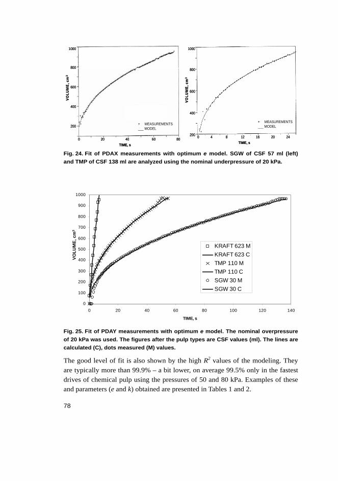
78
Fig. 24. Fit of PDAX measurements with optimum e model. SGW of CSF 57 ml (left)
and TMP of CSF 138 ml are analyzed using the nominal underpressure of 20 kPa.
Fig. 25. Fit of PDAY measurements with optimum e model. The nominal overpressure
of 20 kPa was used. The figures after the pulp types are CSF values (ml). The lines are
calculated (C), dots measured (M) values.
The good level of fit is also shown by the high R2 values of the modeling. They are typically more than 99.9% – a bit lower, on average 99.5% only in the fastest drives of chemical pulp using the pressures of 50 and 80 kPa. Examples of these and parameters (e and k) obtained are presented in Tables 1 and 2.
PDAY 200 mbar
0
100
200
300
400
500
600
700
800
900
1000
0 20 40 60 80 100 120 140
TIME, s
VO
LU
ME
, ml
KRAFT 623 M
KRAFT 623 C
TMP 110 M
TMP 110 C
SGW 30 M
SGW 30 C
PDAY 200 mbar
0
100
200
300
400
500
600
700
800
900
1000
0 20 40 60 80 100 120 140
TIME, s
VO
LU
ME
, ml
KRAFT 623 M
KRAFT 623 C
TMP 110 M
TMP 110 C
SGW 30 M
SGW 30 C
VO
LU
ME
, cm
3
PDAY 200 mbar
0
100
200
300
400
500
600
700
800
900
1000
0 20 40 60 80 100 120 140
TIME, s
VO
LU
ME
, ml
KRAFT 623 M
KRAFT 623 C
TMP 110 M
TMP 110 C
SGW 30 M
SGW 30 C
PDAY 200 mbar
0
100
200
300
400
500
600
700
800
900
1000
0 20 40 60 80 100 120 140
TIME, s
VO
LU
ME
, ml
KRAFT 623 M
KRAFT 623 C
TMP 110 M
TMP 110 C
SGW 30 M
SGW 30 C
VO
LU
ME
, cm
3
200
400
600
800
1000
200
400
600
800
1000
0 20 40 60 800 4 8 12 16 20 24
+ MEASUREMENTS___ MODEL
+ MEASUREMENTS___ MODEL
TIME, sTIME, s
VO
LU
ME
, cm
3
VO
LU
ME
, cm
3
200
400
600
800
1000
200
400
600
800
1000
0 20 40 60 800 4 8 12 16 20 24
+ MEASUREMENTS___ MODEL
+ MEASUREMENTS___ MODEL
TIME, sTIME, s
VO
LU
ME
, cm
3
VO
LU
ME
, cm
3

79
Table 1. Parameters of some PDAX models Ve = kt + V0e.
Pulp type CSF, ml 20 kPa 80 kPa
e k R2 e k R2
SGW 57 2.54 463836 0.9996 2.74 2940885 0.9996
SGW 57 2.66 1143677 0.9996 2.72 2298329 0.9998
PGW 91 2.82 4765355 0.9997 2.89 12812616 0.9991
PGW 91 2.86 6096245 0.9991 3.07 47720392 0.9986
TMP 132 2.85 11646953 0.9988 2.98 39142188 0.9979
TMP 132 2.92 17470969 0.9992 2.98 35760129 0.9984
Table 2. Parameters of some PDAY models Ve = kt + V0e.
Pulp
type
CSF
ml
0 kPa 20 kPa 50 kPa 80 kPa
e k R2 e k R2 e k R2 e k,106 R2
SGW 38 2.11 6716 0.9996 2.12 16898 0.9998 2.15 145468 0.9986 2.60 12300 0.9897
SGW 38 2.19 11437 0.9996 2.14 20340 0.9998 2.40 607024 0.9986 2.41 3390 0.9866
TMP 110 2.28 51257 0.9999 2.25 96415 0.9998 2.40 384797 0.9996 2.38 362 0.9993
TMP 110 2.25 42666 0.9999 2.32 163462 0.9998 2.36 297994 0.9996 2.39 390 0.9994
KRAFT 579 1.20 223 0.9998 1.42 2474 0.9994 1.76 36647 0.9986 2.24 1102 0.9969
KRAFT 579 1.23 266 0.9996 1.41 2275 0.9997 1.66 18571 0.9985 2.02 242 0.9976
8.3.1 Mutual relations between the two parameters of the model
The pulp types SGW, TMP, PGW and chemical pulp are located close to the straight lines of their own and clearly separated from each other on the (lgk, e) plots (Figs. 26 - 31). The lines of the pulp types are in logical order: SGW, PGW, TMP in the PDAX analyses and SGW, TMP, chemical pulp in the PDAY analyses, with the exceptions that SGW mats have been broken by the two highest pressures. The order of parameters e or k (alone) is not as clear but with some reserve one can say that SGW is separated from other mechanical pulps by a lower k value and the chemical pulps from mechanical pulps by a lower e value.
The visual inspection of the Figs. 26 - 31 scarcely shows that the clouds of (lgk, e) points seem to flow up and right when the filtrating pressure increases (excluding SGW of 50 kPa). More clearly the effects of the pressure can be seen by the calculations of the resistance (Ch. 9).

80
Fig. 26. Model parameters of PDAX analyses. The lines were obtained by linear
regresson analysis. The underpressure of 20 kPa was used.
Fig. 27. Model parameters of PDAX analyses. The lines were obtained by linear
regression analysis. The underpressure of 80 kPa was used.
PGW
TMP
SGW
5,0 5,4 5,8 6,2 6,6 7,0 7,4lgk
2,3
2,4
2,5
2,6
2,7
2,8
2,9
3,0
e
PGW
TMP
SGW
5,0 5,4 5,8 6,2 6,6 7,0 7,4lgk
2,3
2,4
2,5
2,6
2,7
2,8
2,9
3,0
e
PGW
SGW
TMP
6,2 6,4 6,6 6,8 7,0 7,2 7,4 7,6lgk
2,6
2,7
2,8
2,9
3,0
3,1
e
PGW
SGW
TMP
6,2 6,4 6,6 6,8 7,0 7,2 7,4 7,6lgk
2,6
2,7
2,8
2,9
3,0
3,1
e
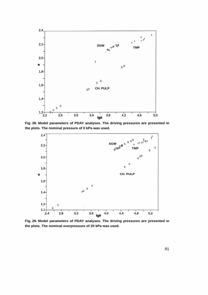
81
Fig. 28. Model parameters of PDAY analyses. The driving pressures are presented in
the plots. The nominal pressure of 0 kPa was used.
Fig. 29. Model parameters of PDAY analyses. The driving pressures are presented in
the plots. The nominal overpressure of 20 kPa was used.
SGW
TMP
CH. PULP
2,4 2,8 3,2 3,6 4,0 4,4 4,8 5,2lgk
1,2
1,1
1,4
1,6
1,8
2,0
2,2
2,4
e
SGW
TMP
CH. PULP
2,4 2,8 3,2 3,6 4,0 4,4 4,8 5,2lgk
1,2
1,1
1,4
1,6
1,8
2,0
2,2
2,4
e
SGWTMP
CH. PULP
2,2 2,6 3,0 3,4 3,8 4,2 4,6 5,0lgk
1,2
1,4
1,6
1,8
2,0
2,2
2,4
e
SGWTMP
CH. PULP
2,2 2,6 3,0 3,4 3,8 4,2 4,6 5,0lgk
1,2
1,4
1,6
1,8
2,0
2,2
2,4
e

82
Fig. 30. Model parameters of PDAY analyses. The driving pressures are presented in
the plots. The nominal overpressure of 50 kPa was used.
Fig. 31. Model parameters of PDAY analyses. The driving pressures are presented in
the plots. The nominal overpressure of 80 kPa was used.
TMP
SGW
CH. PULP
2,5 3,5 4,5 5,5 6,5lgk
1,1
1,2
1,4
1,6
1,8
2,0
2,2
2,4
2,6
e
TMP
SGW
CH. PULP
2,5 3,5 4,5 5,5 6,5lgk
1,1
1,2
1,4
1,6
1,8
2,0
2,2
2,4
2,6
e
TMP
CH. PULP
2,0 4,0 6,0 8,0lgk
0,8
1,0
1,2
1,4
1,6
1,8
2,0
2,2
2,4
2,6
e
TMP
CH. PULP
2,0 4,0 6,0 8,0lgk
0,8
1,0
1,2
1,4
1,6
1,8
2,0
2,2
2,4
2,6
e
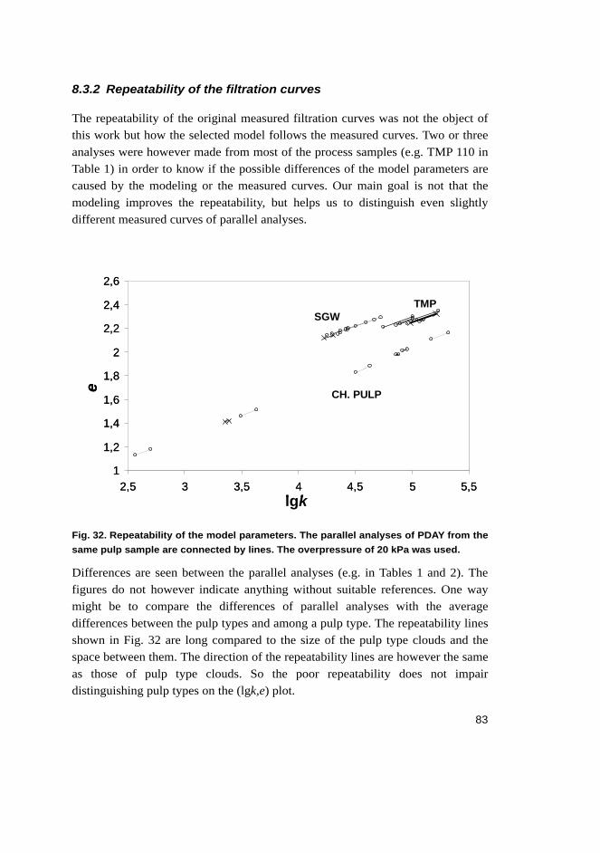
83
8.3.2 Repeatability of the filtration curves
The repeatability of the original measured filtration curves was not the object of this work but how the selected model follows the measured curves. Two or three analyses were however made from most of the process samples (e.g. TMP 110 in Table 1) in order to know if the possible differences of the model parameters are caused by the modeling or the measured curves. Our main goal is not that the modeling improves the repeatability, but helps us to distinguish even slightly different measured curves of parallel analyses.
Fig. 32. Repeatability of the model parameters. The parallel analyses of PDAY from the
same pulp sample are connected by lines. The overpressure of 20 kPa was used.
Differences are seen between the parallel analyses (e.g. in Tables 1 and 2). The figures do not however indicate anything without suitable references. One way might be to compare the differences of parallel analyses with the average differences between the pulp types and among a pulp type. The repeatability lines shown in Fig. 32 are long compared to the size of the pulp type clouds and the space between them. The direction of the repeatability lines are however the same as those of pulp type clouds. So the poor repeatability does not impair distinguishing pulp types on the (lgk,e) plot.
Repeatability, 200 mbar
1
1,2
1,4
1,6
1,8
2
2,2
2,4
2,6
2,5 3 3,5 4 4,5 5 5,5
lgk
e
SGWTMP
CH. PULP
lgk
e
Repeatability, 200 mbar
1
1,2
1,4
1,6
1,8
2
2,2
2,4
2,6
2,5 3 3,5 4 4,5 5 5,5
lgk
e
SGWTMP
CH. PULP
lgk
e

84
The filtration curves of parallel analyses are usually clearly different. The parallel analyses of a TMP sample is presented in Fig. 33. It is the same pair as in Table 2. The curves show that the models follow both of the measured curves more closely than the two measured curves follow each other. The average of the absolute differences between the measured curves is 15.6 cm3, between model curves 15.5 cm3, but only 3.4 cm3 between the measured curve and its model. So the worsening of the repeatability is mainly due to the difference of measured curves and hardly anything due to the modeling.
Fig. 33. The measured (MEAS) and modeled (MODEL) curves of the same pulp sample
(1 and 2). The “MODEL 0” curves are shifted to start from the origin by setting V0e = 0
(in the model Ve = kt +V0e). The (nominal) overpressure has been 20 kPa.
The R2 values were also calculated between the measured and calculated curves of parallel analyses. In spite of the fact that the measured curves of Fig. 33 are visibly different, the correlation between them is very high: R2 = 0.99986. This shows an unknown linear reason that separates the curves as a function of time, which can also be easily seen in Fig. 33. Because at least part of the repeatability
0
100
200
300
400
500
600
700
800
900
1000
0 10 20 30 40 50
TIME, s
FIL
TR
AT
E,
ml
MODEL 0 2
MODEL 0 1
MODEL 2
MEAS 2
MODEL 1
MEAS 1
FIL
TR
AT
ED
VO
LU
ME
, cm
3
0
100
200
300
400
500
600
700
800
900
1000
0 10 20 30 40 50
TIME, s
FIL
TR
AT
E,
ml
MODEL 0 2
MODEL 0 1
MODEL 2
MEAS 2
MODEL 1
MEAS 1
FIL
TR
AT
ED
VO
LU
ME
, cm
3

85
seems to be so deterministic, its source might be worth examining. The correlation between the models and measurements is a bit lower (0.9995 and 0.9996) but between the models’ curves a bit higher (0.99993) probably because the models follow the shape of the measured curves very sharply but are clean of random noise. The highest correlation (0.99998) is however between the model curves shifted to go through the origin by setting V0
e = 0 and thereby eliminating the starting time error. This most easy transformation does not only make the model more simple and understandable but also offers an expedient to improve the repeatability of the filtration curve analyses. It also backs up the usefulness of the additional V0
e term in the model and the deduction that the removing of this term from the equation (after fitting) does not destroy the model. One must however notice the enormous high level of the correlations in the previous.
Another way to illustrate the repeatability is to use for instance the freeness model to scale the differences of parameters to CSF-units (see Chapter 10).
8.4 Alternative means to fit the model to the measurements
The parameters e, k and V0e of the filtration model used in this work (Eq. (8.1))
were calculated by an iterative method: e was given in small steps around e = 2 and the other two parameters were resolved using linear regression analysis. The set of parameters giving the best correlation was selected. Finally the non-informative parameter V0
e was just ignored (Eq. (8.2)) in order to create a situation where all the models of filtration curves start from the origin, which makes the curves more comparable and their mathematical formula simpler and therefore more intelligible.
0e eV kt V (8.1)
eV kt . (8.2)
This fitting method might sound all too complicated for some applications. One way to simplify the model is to resolve time, t from Eq. (8.1) to get Eq. (8.3) and derive the latter as a function of filtrated volume, V in order to get the inverse of volumetric filtration flow rate (dt/dV = 1/qV) as a function of the filtrated volume Eq. (8.4). After finding the logarithm of the equation, the result, Eq. (8.5) is ready for linear regression analysis of variables lg(dt/dV) and lgV in order to resolve the values of (e-1) and lg(e/k), from which it is most easy to calculate the parameters e and k of the model:

86
01 ee V
t Vk k
(8.3)
1dd
et e VV k
(8.4)
dlg 1 lg lgd
t ee VV k . (8.5)
When using either the original or the previous way of fitting, the filtration curve does not need to hit the origin and one does not need to worry about the exact starting time, poor retention, noise or the dominating effect of the screen in the beginning of the drainage. If one however can presuppose that the curve starts at its final shape from the origin, the easiest way of modeling is just to ignore the parameter V0
e already before the fitting. After logarithmic transformation one gets Eq. (8.6) and the values of the expressions (1/e) and (1/e)lgk can be solved by a linear regression analysis program.
1 lglg lg kV te e
. (8.6)
The basic modeling method stated in Chapter 8.1 was used for all the modeled pieces of measured filtration curves in this work. Comparative examples are however calculated for PDAY analyses of the TMP sample using the pressure of 20 kPa. The modeling was done using the same filtrate range (150–900 cm3) as for the basic model in order to get the parameters e and k. Using these parameters the model of the filtration curve was calculated. The correlation coefficients given by these regression analyses are not comparable because of the mathematical transformations before the fitting. So the correlation of measured and modeled values of the filtrate volume as a function of time were calculated as well as the averages of absolute values of errors of the modeled values:
M1 C1 M2 C2 M C. n nAvg err V V V V V V n ,
where VMi and VCi (i = 1,2,…,n) are the measured and calculated filtrated volumes at the same moment, respectively. The results are collected into Table 3 and Figs. 34 and 35.

87
Table 3. Comparison of some modeling of the measured curves. TMP, CSF 110 ml, 20
kPa.
Model e k R2, regr. R2, corr. avg.err., cm3
Ve = kt + V0e 2.25 96415 0.9998 0.9989 3.7
Ve = kt 2.20 71047 0.9960 0.9989 6.7
Ve = kt, shift 0.6 s 2.43 332746 0.9993 0.9993 12.9
Ve = kt, shift 0.2 s 2.25 99891 0.9977 0.9991 5.6
dt/dV, dt = 0.6 s 2.22 77244 0.68 0.9988 17.8
dt/dV, dt = 1.2 s, shift 0.7 s 2.22 77244 0.68 0.9996 30.7
dt/dV, dt = 0.6 s, shift -1.0 s 2.22 77244 0.68 0.9975 9.6
dt/dV, dt = 1.2 s 2.36 200017 0.97 0.9992 11.3
In this special case (TMP, CSF 110 ml, 20 kPa) the simplest model (Eqs. (8.2) and (8.6)) has slightly different values of the model parameters. The filtration curve is a bit less curvy than that of the basic model (Eq. (8.1)) and the measured values. This is shown by the smaller e (2.20 vs. 2.25) in Table 3 and the “kt” curve in Fig. 34. The correlation between the two models and measurements are however very exactly the same. The average error of the simple model is however much greater.

88
Fig. 34. Alternative models of filtration curves are compared to the measured (MEAS)
and the basic ones (Ve = kt + V0e). In the “kt” model the parameter V0
e is just ignored
and in the “dt/dV” model removed by the numerical derivation of the equation before
linearizing it by taking logarithms and using linear regression analysis. Time
differences of 0,6 and 1,2 s are used in the derivation. The pulp type is TMP 110 ml and
the overpressure of 20 kPa is used.
The effect of the starting time error was tested by shifting the sampling time axis before doing the logarithmic transformation and the regression analysis. The maximum correlation between the model and measurements was reached after a delay of 0.6 seconds. The shape of this model curve was more curvy than that of the original model and measurements (Fig. 35). The average of absolute values of errors was more than three-times greater. The minimum average of absolute values of error of the simple model (Ve = kt) was achieved using the shift of 0.2
0
100
200
300
400
500
600
700
800
900
1000
0 10 20 30 40 50
t , s
V,c
m3
dt/dV, 1,2 s
kt
MEAS
BASIC
dt/dV, 0,6 s
dt/dV; 1,2 s
kt
MEAS
BASIC
dt/dV; 0,6 s
0
100
200
300
400
500
600
700
800
900
1000
0 10 20 30 40 50
t , s
V,c
m3
dt/dV, 1,2 s
kt
MEAS
BASIC
dt/dV, 0,6 s
dt/dV; 1,2 s
kt
MEAS
BASIC
dt/dV; 0,6 s

89
seconds. The curvature of the simple model (e) was close to that of the basic model. The correlation with the measurements were slightly better even if the correlation coefficient given by the regression analysis was clearly worse than those of the basic model. The starting time error of 0.5 seconds around these optimum delays has caused an average error of about 5 ml to the filtration curve. The curve of the basic model is shifted 0.1 seconds when the parameter V0
e is removed after modeling.
Fig. 35. Delayed “kt” model compared to the basic model of this work (Ve = kt + V0e).
The time axis of the measurements are shifted (0,0; 0,6 and 1,0 s) before calculating
the “kt”model. The pulp type is TMP 110 ml and the overpressure of 20 kPa is used.
This kind of iterative shifting could also be used as the fitting method and in this particular case has given about the same result as the basic method of this work.
0
100
200
300
400
500
600
700
800
900
1000
0 10 20 30 40 50
t , s
V,
cm3
BASIC
0,0 s
0,6 s
1,0 s

90
The latter however fits the final model with the measurements without any non-linear transformation before the linear regression analysis, which may have dramatic unexpected influences on the model parameters and at least makes the fitting less understandable: The iterative searching for the right curvature (e) is the most natural if the measured curve seems to be more or less curvy than the Darcy’s curve (e = 2). The suitability of the “logarithmic shift” method is however not systematically tested in this work.
The derivative method to model the filtration curve (Eqs. (8.3), (8.4) and (8.5)) was tested using the same data as for the “kt” model. The numerical derivates were calculated using the sample intervals of 0.6 s and 1.2 s:
1
1 1
0,60,6 n nn
n n n n
t tDV V V V
1 1
1 1 1 1
1,21,2 n nn
n n n n
t tDV V V V
,
where Vn is the measured value of the filtrated volume at the moment tn and n = 1,2,…
Fig. 34 shows that the model using the time difference of 0.6 seconds (“dt/dV; 0.6 s”) runs lower than that of the time difference of 1.2 seconds. The basic model and the measurements are located between the models of the two time differences. According to Fig. 34 and Table 3 the former model is less and the latter more curvy than the basic model and the curve of the measurements. The derivation scatters the measurement points (Fig. 36) - wider when the shorter time interval is used. This causes the very bad correlation figures (0.68 and 0.97) of the regression analysis (Table 3). In spite of this poor intermediate result and the visual evaluation of Fig 34, the correlations of the final models and the original measurements are surprisingly good. The average error is also big, meaning that the modeling cannot find the available linear connection between the model and the measurements which is detected by the correlation calculation.

91
Fig. 36. Fit of “dt/dV”-model (C) with the measurements (M) in the logarithmic
coordinates. Both the slope and the deviation are affected by the used time difference
(dt). The pulp type is TMP 110 ml and the overpressure of 20 kPa is used.
It is easy to see (Fig. 37) that the time shift can move the “dt/dV” model curve closer to the measurements. This is done for the model of 0.6 seconds difference. The non-shifted curve of the model is located to the right of the measurements. Therefore the average absolute value of error becomes smaller when the model curve is shifted to the left. The minimum average of absolute values of errors is achieved when the shift to the left is one second (Table 3). The minimum error is however almost 10 cm3 while that of the basic model is less than 4 cm3. Oddly enough, the correlation between the model and the measurements increases when the model curve is pushed to the right, further from the measurements – the relation of the curves becomes more linear even if the distance between them is increasing. The average of absolute values of errors is naturally becoming greater when the model begins to lose touch with the measurements and is as bad as 31 cm3 at the delay of 0.7 s, which gives the maximum correlation, R2 = 0.9996.
-2
-1,8
-1,6
-1,4
-1,2
-1
-0,82,1 2,3 2,5 2,7 2,9
lgV
lg(d
t/d
V)
M, dt = 0,6 s
C, dt = 0,6 s
M, dt = 1,2 s
C, dt = 1,2 s
M, dt = 0,6 s
C, dt = 0,6 s
M, dt = 1,2 s
C, dt = 1,2 s
-2
-1,8
-1,6
-1,4
-1,2
-1
-0,82,1 2,3 2,5 2,7 2,9
lgV
lg(d
t/d
V)
M, dt = 0,6 s
C, dt = 0,6 s
M, dt = 1,2 s
C, dt = 1,2 s
M, dt = 0,6 s
C, dt = 0,6 s
M, dt = 1,2 s
C, dt = 1,2 s
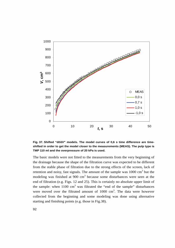
92
Fig. 37. Shifted “dt/dV” models. The model curves of 0,6 s time difference are time-
shifted in order to get the model closer to the measurements (MEAS). The pulp type is
TMP 110 ml and the overpressure of 20 kPa is used.
The basic models were not fitted to the measurements from the very beginning of the drainage because the shape of the filtration curve was expected to be different from the stable phase of filtration due to the strong effects of the screen, lack of retention and noisy, fast signals. The amount of the sample was 1000 cm3 but the modeling was finished at 900 cm3 because some disturbances were seen at the end of filtration (e.g. Figs. 12 and 25). This is certainly no absolute upper limit of the sample: when 1100 cm3 was filtrated the “end of the sample” disturbances were moved over the filtrated amount of 1000 cm3. The data were however collected from the beginning and some modeling was done using alternative starting and finishing points (e.g. those in Fig.38).
0
100
200
300
400
500
600
700
800
900
1000
0 10 20 30 40 50
t, s
V, m
l
MEAS
0,0 s
0,7 s
1,0 s
-1,0 s
V,
cm3
0
100
200
300
400
500
600
700
800
900
1000
0 10 20 30 40 50
t, s
V, m
l
MEAS
0,0 s
0,7 s
1,0 s
-1,0 s
V,
cm3
t, s
V,
cm3
0
100
200
300
400
500
600
700
800
900
1000
0 10 20 30 40 50
t, s
V, m
l
MEAS
0,0 s
0,7 s
1,0 s
-1,0 s
V,
cm3
0
100
200
300
400
500
600
700
800
900
1000
0 10 20 30 40 50
t, s
V, m
l
MEAS
0,0 s
0,7 s
1,0 s
-1,0 s
V,
cm3
t, s
V,
cm3

93
Fig. 38. Alternative fitting ranges of filtrated volume in the modeling. The effects of the
starting (SP) and finishing points are presented. E.g., the range of the analysis SP 400
cm3 has been 400–900 cm3 and that of FP 400 has been 0–400 cm3. The overpressure
has been 20 kPa and CSF values 33, 124 and 584 ml.
When the fitting range has been expanded keeping the starting point at zero, the value of the curvature parameter e is typically increased. Narrowing the range from the widest value (0–900 cm3) by increasing the starting point (e.g. to 200–900 cm3) seems not to have changed the parameter e very much perhaps because the huge majority of the measured data have been at the slow end of filtration. The highest correlation values are usually achieved when the range is started from 100–200 cm3 if it is finished at 900 cm3 – evidently because of the disturbances and the effect of wire in the beginning of the filtration. The final phase is also noisy and the shape of the curve changes (Fig. 12) – there might be turbulences, even splashes and finally the fiber mat is seen by the level sensor.
0,50
0,70
0,90
1,10
1,30
1,50
1,70
1,90
2,10
2,30
2,50
0 200 400 600 800 1000
V , ml
eKRAFT 584 SP
KRAFT 584 FP
TMP 124 SP
TMP 124 FP
SGW 33 SP
SGW 33 FP

94

95
9 Experimental models of resistance
The model of the filtration curve used in this work has had a good fit with the measurements made by two analyzers with many driving pressures for different kinds of pulp types. The shape and thereby the information of the filtration curves are managed to pack into two parameters, e and k of the equation Ve = kt. This is the main result of this thesis. However, no matter how good the model of the filtration curve is and how important it is as an information link of the measurement chain, alone it is just a nice function of time generated by a self-made apparatus or only two figures. They may be worth being compared with each other especially if keeping in mind the main properties and conditions of the analyzers. But they have no straight and unambiguous connection to the real object of interest: pulp properties. A more general and without question most important property of pulp is the specific resistance, which demonstrates how the pad made of a certain pulp resists liquid flow through it, when the values of grammage and area of the pad as well as the dynamic viscosity of the fluid are unit. A formula to calculate the specific resistances (RS and RSη) from the measurements can be solved from Eq. (7.16) by substituting the grammage W = VC0, the volume flow rate qV = dV/dt and separating the viscosity (η) of the liquid from the specific resistance RS = ηRSη:
2
SS
0
R AR pdVVCdt
. (9.1)
Instead of managing the measured filtration curves, which are noisy and consist of numerous pairs of figures, after knowing the two parameters of the model, the specific resistance can be studied (e.g.) by applying Eq. (7.17) and including the viscosity (η) in the formula:
2
2S
0
eA eR pVC k
. (9.2)
If the area of the pulp pad (A), the consistency of the sample (C0), viscosity of the flowing liquid (η) and even the driving pressure are constant during the filtration, the parameter e describes the tendency of the specific resistance during the course of the drainage. The specific resistance increases when e > 2 and decreases when e < 2. The modeling based on the measurements of PDAX and PDAY have given different e values far from 2, suggesting that the pulp pads do not follow Darcy’s

96
law and that the value of e must be specified by (experimental) fitting of the model to the measurements instead of just adapting the regular value e = 2. It is unlikely that the multipliers of V are constant (enough) even within the limited modeling range of the filtrated volume. It is still more unlikely that changes of the multipliers happen to be suitable to compensate all the differences between the measured curves and Darcy’s curves. The consistency of the sample (C0) and the area of the mat (A) are supposed to be constant but the driving pressure (Δp) is measured as a function of time and thereby also as a function of filtrated volume in order to calculate the progress of the specific filtration resistance.
9.1 Filtrating pressure
Even according to Darcy’s law, the parameter e of our filtration model must differ from two if the pressure is not constant but the specific filtration resistance should be independent of filtration time, filtrated volume and driving pressure. And the pressure has not been constant (Fig. 39)!
Fig. 39. The driving pressure of PDAY as a function of filtration time (t) and filtrated
volume (V), when the gauge pressure of the air container, “nominal overpressure” was
20 kPa. The CSF values of the pulps were 38, 110 and 472 ml.
The filtration has been driven by the sum of gauge pressure of the air container (pc), hydrostatic pressure of the sample and filtrate in PDAY (ph) and the pressure due to acceleration (pr):
c h rp p p p . (9.3)
SGW 38
TMP 110
KRAFT 472
21,5
22
22,5
23
23,5
24
24,5
25
0 20 40 60 80 100 120
t, s
P, k
Pa
SGW
KRAFT
21,5
22
22,5
23
23,5
24
24,5
25
0 200 400 600 800 1000
V, cm3
P, k
Pa
SGW 38
TMP 110
KRAFT 472
SGW 38
TMP 110
KRAFT 472
21,5
22
22,5
23
23,5
24
24,5
25
0 20 40 60 80 100 120
t, s
P, k
Pa
SGW
KRAFT
21,5
22
22,5
23
23,5
24
24,5
25
0 200 400 600 800 1000
V, cm3
P, k
Pa
SGW 38
TMP 110
KRAFT 472
V, cm3t, s
∆p
, kP
a
∆p
, kP
a
SGW 38
TMP 110
KRAFT 472
21,5
22
22,5
23
23,5
24
24,5
25
0 20 40 60 80 100 120
t, s
P, k
Pa
SGW
KRAFT
21,5
22
22,5
23
23,5
24
24,5
25
0 200 400 600 800 1000
V, cm3
P, k
Pa
SGW 38
TMP 110
KRAFT 472
SGW 38
TMP 110
KRAFT 472
21,5
22
22,5
23
23,5
24
24,5
25
0 20 40 60 80 100 120
t, s
P, k
Pa
SGW
KRAFT
21,5
22
22,5
23
23,5
24
24,5
25
0 200 400 600 800 1000
V, cm3
P, k
Pa
SGW 38
TMP 110
KRAFT 472
V, cm3t, s
∆p
, kP
a
∆p
, kP
a

97
This is the pressure difference over the pad on the screen during the filtration, when the pressure drops in the air and filtrate tubes as well as over the screen are negligible. Both the air and hydrostatic pressures affect in the same direction as a driving pressure and have positive values. The used gauge pressure levels or the initial pressures of the container were 0 (PDAY only), 20, 50 (PDAY only) and 80 kPa. The analyses are referred to in the text as these nominal levels (e.g. 50 kPa). These levels were carried out by the pressure of air stored in a large (75 dm3) container in order to keep the pressure as constant as possible in spite of the fact that the air volume was decreasing in PDAX and increasing in PDAY with the increase of the filtrated volume. The air pressure was either the low pressure (vacuum) below the screen in PDAX or the high pressure above the sample in PDAY. These gauge pressures are relative to the local atmospheric pressure of outside the equipment. Both of these were measured in the air containers. There was a stepwise drop in the beginning of drainages when the container is connected to the chamber of the sample or the filtrate. This drop was independent of the pulp type and the speed of filtration. The step can be seen when the pressure is plotted as a function of time but not when it is plotted as a function of the filtrated volume (Fig. 39). It would have been easy to minimize in PDAY just by minimizing the empty volume above the surface in the sample chamber – most easily by increasing the amount of the sample. This step was immediately followed by the decreasing fall caused by the flow of filtrate from the sample chamber to the filtrate chamber. It was almost linear and independent of (the freeness of) the pulp type when described as a function of the filtrated volume (or grammage, W). However the fast almost adiabatic change of the air volume in the beginning of the filtration suddenly changes the temperature of the air container. The height of this temperature jump is dependent also on the speed of the filtration. The temperature gradually creeps towards its original value or the temperature of the surrounding room. The slower the filtration, the higher the increase of the pressure at a certain volume of the filtrate due to this temperature reversion (SGW vs. KRAFT in Fig 39) while it should be the same at the same time for all sorts of pulps. As unsophisticated as it might appear, the use of an air pressure container and large enough sample vessel offers thus a possibility to compensate for the decrease of the pressure caused by the filtrate flow! This is not however systematically utilized in this equipment.
The hydrostatic pressure (ph) was caused by the sample both in PDAX and PDAY – in PDAY additionally by the liquid below (the sample and) the screen. Both of these can be calculated from the measurements (and the model) of the

98
filtrated volume knowing the diameters of the sample vessels and that the height of the liquid below the screen is kept even by overflow and supposing that there are continuous liquid paths through the pulp mat on the screen.
The liquid around the screen must be first accelerated from the rest and its mass causes negative (pr < 0 in Eq. 9.3) pressure but the acceleration turns to the retardation and the pressure to positive before the modeling range of this study. The retardation was at its maximum in the beginning of the modeling area (V = 150 cm3 in PDAY) and when analyzing the pulps of the fastest dewatering using the highest pressure (80 kPa), but in all cases the pressure was insignificant (less than 0.1% of the total pressure).
In the case of the “0 kPa” trials, only hydrostatic pressure was used and the total pressure can be calculated without any pressure sensors.
Thus the driving pressure was the sum of the air pressure and the hydrostatic pressure. The pressure is decreasing during the course of the drainage. The pressure curves are clearly different as a function of time but they would be alike without the temperature change of the pressurized air – if the process would be isothermic enough.
When the values of the filtration volume (V) and the pressure are known as a function of time, the specific resistance can be calculated as a function of time, filtration volume and grammage. One must however keep in mind that the specific resistance is affected not only by the momentary value but the total history of the pressure – by both the height and the duration of the action, which are also dependent on the dewaterability of the pulp. Many pressure levels are used to see at least the clear influences of the pressure on the filtration and resistance curves and on their models. It is outside of the scope of this work to quantitatively evaluate what kind of filtration curves and model parameters would have been generated by different kinds of pressure curves (e.g. by constant pressure). It has been contented with the examination and comparison of the very curves produced by our two systems and their models.
9.2 Trends of the specific resistance
The models of the filtration curves are used to illustrate the differences of the progress of the specific resistance when different types of pulps are drained using different pressure levels. In Fig. 40, typical curves of the specific resistance are presented. Higher pressures have produced generally more resistive pads than lower pressures. The two highest pressures have however dropped the resistance
99
of SGW – the mat is too weak to stand pressures which are that high in addition to the heavy flow of filtrate. The CSF value of 38 ml is so low that the pulp must have been ground to a quite “powder-like” extent. According to the laboratory analyses, the fines content is high and the tear index low.
The specific resistance of the mechanical pulps have usually increased during the course of the filtration – when new material is fed into the pad. The chemical pulps had the same common trend when high pressures were used but during low pressure filtrations the mats of the chemical pulps become less and less resistive – so to say, sparser. If the freeness of the chemical pulp was very high (kraft 835 ml in Fig. 40) not even the highest pressures of these analyses could press the new material tighter and tighter into the mat but the resistance was decreasing during the course of the drainage. Probably there has been very little fines material to fill the holes and the long fibers have not been flexible enough to bend into the holes of the pad.
The specific resistances have also changed during the drainage but the driving pressures have changed too. It has also been seen that the specific resistances have been strongly affected by the pressure. So we can be sure that the pad has not been darcy-like under these conditions of changing pressure. Could it however be possible that the constant pressure would have produced a mat of constant specific resistance? In that case the parameter e of our model should have been two. Most of the specific resistances have increased during the drainage. If we think that the decrease of the driving pressure would have finished at a certain filtrated volume and would have been constant after that, the rest of the filtration would have been carried out using higher pressure than the original, real filtration. It has been seen that higher pressures produce higher specific resistances. So it is evident that the constant (higher) pressure tail of the filtration would have produced even more increasing specific resistance than the original decreasing pressure. It means that the filtration curve (V(t)) would have been more curvy and the exponent of our model would have differed from two even more than that of the original model. We cannot however know, how good the fit between the model and measurements would have been if the pressure would have been constant.

100
Fig. 40. Calculated specific resistances based on the models of filtration curves and
measurements of the gauge overpressures in the air container. SGW of 38 ml CSF in
the left upper, TMP of 110 ml in the right upper, chemical pulp of 472 ml in the left
lower and chemical pulp of 635 ml in the right lower corner. For TMP also the
repeatability of the two parallel analyses is shown.
The decreasing specific resistance curves would surely have turned more horizontal and some of them even increasing if the pressure would not have been decreasing, but constant. How much higher the tail of the curve could be, can be roughly evaluated using the adjacent pressure curves. Let us examine, e.g. the PDAY drive of the chemical pulp, CSF 635 ml with the pressure level 20 kPa. The lowering of the pressure is less than 3 kPa during the drainage. It is 10% of the difference between the pressures of the drives of 50 and 20 kPa. If the initial pressure would have been 23 kPa instead of 20 kPa, the curve of the specific resistance would certainly have been located between the specific resistance curves of the pressures 20 and 50 kPa – probably about 10% of the cap higher than the curve of 20 kPa. Although the end of the 20 kPa curve in Fig. 40 is lifted by the 10% of the gap, it stays much lower than the beginning of the 20 kPa curve. The effect of the constant pressure must have been smaller. We can be sure that
0,8 bar
0,5 bar
0,2 bar
0,0 bar
0
20
40
60
80
100
120
140
160
180
0 200 400 600 800 1000
V, ml
Rsn
C, 1
09 m
/kg
0,8 bar
0,5 bar
0,2 bar
0,0 bar
0
20
40
60
80
100
120
140
160
0 200 400 600 800 1000
V, ml
Rsn
C, 1
09 m
/kg
0,8 bar
0,5 bar
0,2 bar
0,0 bar
0
5
10
15
20
25
30
35
0 200 400 600 800 1000
V, ml
Rsn
, 10
9 m
/kg
0,0 bar
0,2 bar
0,5 bar
0,8 bar
0
5
10
15
20
25
0 200 400 600 800 1000
V, ml
Rsn
C, 1
09 m
/kg
0,8 bar
0,5 bar
0,2 bar
0,0 bar
0
20
40
60
80
100
120
140
160
180
0 200 400 600 800 1000
V, ml
Rsn
C, 1
09 m
/kg
0,8 bar
0,5 bar
0,2 bar
0,0 bar
0
20
40
60
80
100
120
140
160
0 200 400 600 800 1000
V, ml
Rsn
C, 1
09 m
/kg
0,8 bar
0,5 bar
0,2 bar
0,0 bar
0
5
10
15
20
25
30
35
0 200 400 600 800 1000
V, ml
Rsn
, 10
9 m
/kg
0,0 bar
0,2 bar
0,5 bar
0,8 bar
0
5
10
15
20
25
0 200 400 600 800 1000
V, ml
Rsn
C, 1
09 m
/kg
20 kPa
0 kPa
50 kPa
80 kPa 0 kPa
20 kPa
50 kPa
80 kPa
80 kPa50 kPa
20 kPa
0 kPa
80 kPa
50 kPa
20 kPa
0 kPa
V, cm3 V, cm3
V, cm3 V, cm3
0,8 bar
0,5 bar
0,2 bar
0,0 bar
0
20
40
60
80
100
120
140
160
180
0 200 400 600 800 1000
V, ml
Rsn
C, 1
09 m
/kg
0,8 bar
0,5 bar
0,2 bar
0,0 bar
0
20
40
60
80
100
120
140
160
0 200 400 600 800 1000
V, ml
Rsn
C, 1
09 m
/kg
0,8 bar
0,5 bar
0,2 bar
0,0 bar
0
5
10
15
20
25
30
35
0 200 400 600 800 1000
V, ml
Rsn
, 10
9 m
/kg
0,0 bar
0,2 bar
0,5 bar
0,8 bar
0
5
10
15
20
25
0 200 400 600 800 1000
V, ml
Rsn
C, 1
09 m
/kg
0,8 bar
0,5 bar
0,2 bar
0,0 bar
0
20
40
60
80
100
120
140
160
180
0 200 400 600 800 1000
V, ml
Rsn
C, 1
09 m
/kg
0,8 bar
0,5 bar
0,2 bar
0,0 bar
0
20
40
60
80
100
120
140
160
0 200 400 600 800 1000
V, ml
Rsn
C, 1
09 m
/kg
0,8 bar
0,5 bar
0,2 bar
0,0 bar
0
5
10
15
20
25
30
35
0 200 400 600 800 1000
V, ml
Rsn
, 10
9 m
/kg
0,0 bar
0,2 bar
0,5 bar
0,8 bar
0
5
10
15
20
25
0 200 400 600 800 1000
V, ml
Rsn
C, 1
09 m
/kg
20 kPa
0 kPa
50 kPa
80 kPa 0 kPa
20 kPa
50 kPa
80 kPa
80 kPa50 kPa
20 kPa
0 kPa
80 kPa
50 kPa
20 kPa
0 kPa
0,8 bar
0,5 bar
0,2 bar
0,0 bar
0
20
40
60
80
100
120
140
160
180
0 200 400 600 800 1000
V, ml
Rsn
C, 1
09 m
/kg
0,8 bar
0,5 bar
0,2 bar
0,0 bar
0
20
40
60
80
100
120
140
160
0 200 400 600 800 1000
V, ml
Rsn
C, 1
09 m
/kg
0,8 bar
0,5 bar
0,2 bar
0,0 bar
0
5
10
15
20
25
30
35
0 200 400 600 800 1000
V, ml
Rsn
, 10
9 m
/kg
0,0 bar
0,2 bar
0,5 bar
0,8 bar
0
5
10
15
20
25
0 200 400 600 800 1000
V, ml
Rsn
C, 1
09 m
/kg
0,8 bar
0,5 bar
0,2 bar
0,0 bar
0
20
40
60
80
100
120
140
160
180
0 200 400 600 800 1000
V, ml
Rsn
C, 1
09 m
/kg
0,8 bar
0,5 bar
0,2 bar
0,0 bar
0
20
40
60
80
100
120
140
160
0 200 400 600 800 1000
V, ml
Rsn
C, 1
09 m
/kg
0,8 bar
0,5 bar
0,2 bar
0,0 bar
0
5
10
15
20
25
30
35
0 200 400 600 800 1000
V, ml
Rsn
, 10
9 m
/kg
0,0 bar
0,2 bar
0,5 bar
0,8 bar
0
5
10
15
20
25
0 200 400 600 800 1000
V, ml
Rsn
C, 1
09 m
/kg
20 kPa
0 kPa
50 kPa
80 kPa 0 kPa
20 kPa
50 kPa
80 kPa
80 kPa50 kPa
20 kPa
0 kPa
80 kPa
50 kPa
20 kPa
0 kPa
V, cm3 V, cm3
V, cm3 V, cm3
V, cm3V, cm3
V, cm3 V, cm3
RSη
C, 1
09m
/kg
RSη
C, 1
09
m/k
g
RSη
C, 1
09
m/k
gR
Sη
C, 1
09
m/k
g
0,8 bar
0,5 bar
0,2 bar
0,0 bar
0
20
40
60
80
100
120
140
160
180
0 200 400 600 800 1000
V, ml
Rsn
C, 1
09 m
/kg
0,8 bar
0,5 bar
0,2 bar
0,0 bar
0
20
40
60
80
100
120
140
160
0 200 400 600 800 1000
V, ml
Rsn
C, 1
09 m
/kg
0,8 bar
0,5 bar
0,2 bar
0,0 bar
0
5
10
15
20
25
30
35
0 200 400 600 800 1000
V, ml
Rsn
, 10
9 m
/kg
0,0 bar
0,2 bar
0,5 bar
0,8 bar
0
5
10
15
20
25
0 200 400 600 800 1000
V, ml
Rsn
C, 1
09 m
/kg
0,8 bar
0,5 bar
0,2 bar
0,0 bar
0
20
40
60
80
100
120
140
160
180
0 200 400 600 800 1000
V, ml
Rsn
C, 1
09 m
/kg
0,8 bar
0,5 bar
0,2 bar
0,0 bar
0
20
40
60
80
100
120
140
160
0 200 400 600 800 1000
V, ml
Rsn
C, 1
09 m
/kg
0,8 bar
0,5 bar
0,2 bar
0,0 bar
0
5
10
15
20
25
30
35
0 200 400 600 800 1000
V, ml
Rsn
, 10
9 m
/kg
0,0 bar
0,2 bar
0,5 bar
0,8 bar
0
5
10
15
20
25
0 200 400 600 800 1000
V, ml
Rsn
C, 1
09 m
/kg
20 kPa
0 kPa
50 kPa
80 kPa 0 kPa
20 kPa
50 kPa
80 kPa
80 kPa50 kPa
20 kPa
0 kPa
80 kPa
50 kPa
20 kPa
0 kPa
V, cm3 V, cm3
V, cm3 V, cm3
0,8 bar
0,5 bar
0,2 bar
0,0 bar
0
20
40
60
80
100
120
140
160
180
0 200 400 600 800 1000
V, ml
Rsn
C, 1
09 m
/kg
0,8 bar
0,5 bar
0,2 bar
0,0 bar
0
20
40
60
80
100
120
140
160
0 200 400 600 800 1000
V, ml
Rsn
C, 1
09 m
/kg
0,8 bar
0,5 bar
0,2 bar
0,0 bar
0
5
10
15
20
25
30
35
0 200 400 600 800 1000
V, ml
Rsn
, 10
9 m
/kg
0,0 bar
0,2 bar
0,5 bar
0,8 bar
0
5
10
15
20
25
0 200 400 600 800 1000
V, ml
Rsn
C, 1
09 m
/kg
0,8 bar
0,5 bar
0,2 bar
0,0 bar
0
20
40
60
80
100
120
140
160
180
0 200 400 600 800 1000
V, ml
Rsn
C, 1
09 m
/kg
0,8 bar
0,5 bar
0,2 bar
0,0 bar
0
20
40
60
80
100
120
140
160
0 200 400 600 800 1000
V, ml
Rsn
C, 1
09 m
/kg
0,8 bar
0,5 bar
0,2 bar
0,0 bar
0
5
10
15
20
25
30
35
0 200 400 600 800 1000
V, ml
Rsn
, 10
9 m
/kg
0,0 bar
0,2 bar
0,5 bar
0,8 bar
0
5
10
15
20
25
0 200 400 600 800 1000
V, ml
Rsn
C, 1
09 m
/kg
20 kPa
0 kPa
50 kPa
80 kPa 0 kPa
20 kPa
50 kPa
80 kPa
80 kPa50 kPa
20 kPa
0 kPa
80 kPa
50 kPa
20 kPa
0 kPa
0,8 bar
0,5 bar
0,2 bar
0,0 bar
0
20
40
60
80
100
120
140
160
180
0 200 400 600 800 1000
V, ml
Rsn
C, 1
09 m
/kg
0,8 bar
0,5 bar
0,2 bar
0,0 bar
0
20
40
60
80
100
120
140
160
0 200 400 600 800 1000
V, ml
Rsn
C, 1
09 m
/kg
0,8 bar
0,5 bar
0,2 bar
0,0 bar
0
5
10
15
20
25
30
35
0 200 400 600 800 1000
V, ml
Rsn
, 10
9 m
/kg
0,0 bar
0,2 bar
0,5 bar
0,8 bar
0
5
10
15
20
25
0 200 400 600 800 1000
V, ml
Rsn
C, 1
09 m
/kg
0,8 bar
0,5 bar
0,2 bar
0,0 bar
0
20
40
60
80
100
120
140
160
180
0 200 400 600 800 1000
V, ml
Rsn
C, 1
09 m
/kg
0,8 bar
0,5 bar
0,2 bar
0,0 bar
0
20
40
60
80
100
120
140
160
0 200 400 600 800 1000
V, ml
Rsn
C, 1
09 m
/kg
0,8 bar
0,5 bar
0,2 bar
0,0 bar
0
5
10
15
20
25
30
35
0 200 400 600 800 1000
V, ml
Rsn
, 10
9 m
/kg
0,0 bar
0,2 bar
0,5 bar
0,8 bar
0
5
10
15
20
25
0 200 400 600 800 1000
V, ml
Rsn
C, 1
09 m
/kg
20 kPa
0 kPa
50 kPa
80 kPa 0 kPa
20 kPa
50 kPa
80 kPa
80 kPa50 kPa
20 kPa
0 kPa
80 kPa
50 kPa
20 kPa
0 kPa
V, cm3 V, cm3
V, cm3 V, cm3
V, cm3V, cm3
V, cm3 V, cm3
RSη
C, 1
09m
/kg
RSη
C, 1
09
m/k
g
RSη
C, 1
09
m/k
gR
Sη
C, 1
09
m/k
g
RSη
C,10
9m
/kg
RSη
C,10
9m
/kg
RSη
C,10
9m
/kg
RSη
C,10
9m
/kg
0,8 bar
0,5 bar
0,2 bar
0,0 bar
0
20
40
60
80
100
120
140
160
180
0 200 400 600 800 1000
V, ml
Rsn
C, 1
09 m
/kg
0,8 bar
0,5 bar
0,2 bar
0,0 bar
0
20
40
60
80
100
120
140
160
0 200 400 600 800 1000
V, ml
Rsn
C, 1
09 m
/kg
0,8 bar
0,5 bar
0,2 bar
0,0 bar
0
5
10
15
20
25
30
35
0 200 400 600 800 1000
V, ml
Rsn
, 10
9 m
/kg
0,0 bar
0,2 bar
0,5 bar
0,8 bar
0
5
10
15
20
25
0 200 400 600 800 1000
V, ml
Rsn
C, 1
09 m
/kg
0,8 bar
0,5 bar
0,2 bar
0,0 bar
0
20
40
60
80
100
120
140
160
180
0 200 400 600 800 1000
V, ml
Rsn
C, 1
09 m
/kg
0,8 bar
0,5 bar
0,2 bar
0,0 bar
0
20
40
60
80
100
120
140
160
0 200 400 600 800 1000
V, ml
Rsn
C, 1
09 m
/kg
0,8 bar
0,5 bar
0,2 bar
0,0 bar
0
5
10
15
20
25
30
35
0 200 400 600 800 1000
V, ml
Rsn
, 10
9 m
/kg
0,0 bar
0,2 bar
0,5 bar
0,8 bar
0
5
10
15
20
25
0 200 400 600 800 1000
V, ml
Rsn
C, 1
09 m
/kg
20 kPa
0 kPa
50 kPa
80 kPa 0 kPa
20 kPa
50 kPa
80 kPa
80 kPa50 kPa
20 kPa
0 kPa
80 kPa
50 kPa
20 kPa
0 kPa
V, cm3 V, cm3
V, cm3 V, cm3
0,8 bar
0,5 bar
0,2 bar
0,0 bar
0
20
40
60
80
100
120
140
160
180
0 200 400 600 800 1000
V, ml
Rsn
C, 1
09 m
/kg
0,8 bar
0,5 bar
0,2 bar
0,0 bar
0
20
40
60
80
100
120
140
160
0 200 400 600 800 1000
V, ml
Rsn
C, 1
09 m
/kg
0,8 bar
0,5 bar
0,2 bar
0,0 bar
0
5
10
15
20
25
30
35
0 200 400 600 800 1000
V, ml
Rsn
, 10
9 m
/kg
0,0 bar
0,2 bar
0,5 bar
0,8 bar
0
5
10
15
20
25
0 200 400 600 800 1000
V, ml
Rsn
C, 1
09 m
/kg
0,8 bar
0,5 bar
0,2 bar
0,0 bar
0
20
40
60
80
100
120
140
160
180
0 200 400 600 800 1000
V, ml
Rsn
C, 1
09 m
/kg
0,8 bar
0,5 bar
0,2 bar
0,0 bar
0
20
40
60
80
100
120
140
160
0 200 400 600 800 1000
V, ml
Rsn
C, 1
09 m
/kg
0,8 bar
0,5 bar
0,2 bar
0,0 bar
0
5
10
15
20
25
30
35
0 200 400 600 800 1000
V, ml
Rsn
, 10
9 m
/kg
0,0 bar
0,2 bar
0,5 bar
0,8 bar
0
5
10
15
20
25
0 200 400 600 800 1000
V, ml
Rsn
C, 1
09 m
/kg
20 kPa
0 kPa
50 kPa
80 kPa 0 kPa
20 kPa
50 kPa
80 kPa
80 kPa50 kPa
20 kPa
0 kPa
80 kPa
50 kPa
20 kPa
0 kPa
0,8 bar
0,5 bar
0,2 bar
0,0 bar
0
20
40
60
80
100
120
140
160
180
0 200 400 600 800 1000
V, ml
Rsn
C, 1
09 m
/kg
0,8 bar
0,5 bar
0,2 bar
0,0 bar
0
20
40
60
80
100
120
140
160
0 200 400 600 800 1000
V, ml
Rsn
C, 1
09 m
/kg
0,8 bar
0,5 bar
0,2 bar
0,0 bar
0
5
10
15
20
25
30
35
0 200 400 600 800 1000
V, ml
Rsn
, 10
9 m
/kg
0,0 bar
0,2 bar
0,5 bar
0,8 bar
0
5
10
15
20
25
0 200 400 600 800 1000
V, ml
Rsn
C, 1
09 m
/kg
0,8 bar
0,5 bar
0,2 bar
0,0 bar
0
20
40
60
80
100
120
140
160
180
0 200 400 600 800 1000
V, ml
Rsn
C, 1
09 m
/kg
0,8 bar
0,5 bar
0,2 bar
0,0 bar
0
20
40
60
80
100
120
140
160
0 200 400 600 800 1000
V, ml
Rsn
C, 1
09 m
/kg
0,8 bar
0,5 bar
0,2 bar
0,0 bar
0
5
10
15
20
25
30
35
0 200 400 600 800 1000
V, ml
Rsn
, 10
9 m
/kg
0,0 bar
0,2 bar
0,5 bar
0,8 bar
0
5
10
15
20
25
0 200 400 600 800 1000
V, ml
Rsn
C, 1
09 m
/kg
20 kPa
0 kPa
50 kPa
80 kPa 0 kPa
20 kPa
50 kPa
80 kPa
80 kPa50 kPa
20 kPa
0 kPa
80 kPa
50 kPa
20 kPa
0 kPa
V, cm3 V, cm3
V, cm3 V, cm3
V, cm3V, cm3
V, cm3 V, cm3
RSη
C, 1
09m
/kg
RSη
C, 1
09
m/k
g
RSη
C, 1
09
m/k
gR
Sη
C, 1
09
m/k
g
0,8 bar
0,5 bar
0,2 bar
0,0 bar
0
20
40
60
80
100
120
140
160
180
0 200 400 600 800 1000
V, ml
Rsn
C, 1
09 m
/kg
0,8 bar
0,5 bar
0,2 bar
0,0 bar
0
20
40
60
80
100
120
140
160
0 200 400 600 800 1000
V, ml
Rsn
C, 1
09 m
/kg
0,8 bar
0,5 bar
0,2 bar
0,0 bar
0
5
10
15
20
25
30
35
0 200 400 600 800 1000
V, ml
Rsn
, 10
9 m
/kg
0,0 bar
0,2 bar
0,5 bar
0,8 bar
0
5
10
15
20
25
0 200 400 600 800 1000
V, ml
Rsn
C, 1
09 m
/kg
0,8 bar
0,5 bar
0,2 bar
0,0 bar
0
20
40
60
80
100
120
140
160
180
0 200 400 600 800 1000
V, ml
Rsn
C, 1
09 m
/kg
0,8 bar
0,5 bar
0,2 bar
0,0 bar
0
20
40
60
80
100
120
140
160
0 200 400 600 800 1000
V, ml
Rsn
C, 1
09 m
/kg
0,8 bar
0,5 bar
0,2 bar
0,0 bar
0
5
10
15
20
25
30
35
0 200 400 600 800 1000
V, ml
Rsn
, 10
9 m
/kg
0,0 bar
0,2 bar
0,5 bar
0,8 bar
0
5
10
15
20
25
0 200 400 600 800 1000
V, ml
Rsn
C, 1
09 m
/kg
20 kPa
0 kPa
50 kPa
80 kPa 0 kPa
20 kPa
50 kPa
80 kPa
80 kPa50 kPa
20 kPa
0 kPa
80 kPa
50 kPa
20 kPa
0 kPa
V, cm3 V, cm3
V, cm3 V, cm3
0,8 bar
0,5 bar
0,2 bar
0,0 bar
0
20
40
60
80
100
120
140
160
180
0 200 400 600 800 1000
V, ml
Rsn
C, 1
09 m
/kg
0,8 bar
0,5 bar
0,2 bar
0,0 bar
0
20
40
60
80
100
120
140
160
0 200 400 600 800 1000
V, ml
Rsn
C, 1
09 m
/kg
0,8 bar
0,5 bar
0,2 bar
0,0 bar
0
5
10
15
20
25
30
35
0 200 400 600 800 1000
V, ml
Rsn
, 10
9 m
/kg
0,0 bar
0,2 bar
0,5 bar
0,8 bar
0
5
10
15
20
25
0 200 400 600 800 1000
V, ml
Rsn
C, 1
09 m
/kg
0,8 bar
0,5 bar
0,2 bar
0,0 bar
0
20
40
60
80
100
120
140
160
180
0 200 400 600 800 1000
V, ml
Rsn
C, 1
09 m
/kg
0,8 bar
0,5 bar
0,2 bar
0,0 bar
0
20
40
60
80
100
120
140
160
0 200 400 600 800 1000
V, ml
Rsn
C, 1
09 m
/kg
0,8 bar
0,5 bar
0,2 bar
0,0 bar
0
5
10
15
20
25
30
35
0 200 400 600 800 1000
V, ml
Rsn
, 10
9 m
/kg
0,0 bar
0,2 bar
0,5 bar
0,8 bar
0
5
10
15
20
25
0 200 400 600 800 1000
V, ml
Rsn
C, 1
09 m
/kg
20 kPa
0 kPa
50 kPa
80 kPa 0 kPa
20 kPa
50 kPa
80 kPa
80 kPa50 kPa
20 kPa
0 kPa
80 kPa
50 kPa
20 kPa
0 kPa
0,8 bar
0,5 bar
0,2 bar
0,0 bar
0
20
40
60
80
100
120
140
160
180
0 200 400 600 800 1000
V, ml
Rsn
C, 1
09 m
/kg
0,8 bar
0,5 bar
0,2 bar
0,0 bar
0
20
40
60
80
100
120
140
160
0 200 400 600 800 1000
V, ml
Rsn
C, 1
09 m
/kg
0,8 bar
0,5 bar
0,2 bar
0,0 bar
0
5
10
15
20
25
30
35
0 200 400 600 800 1000
V, ml
Rsn
, 10
9 m
/kg
0,0 bar
0,2 bar
0,5 bar
0,8 bar
0
5
10
15
20
25
0 200 400 600 800 1000
V, ml
Rsn
C, 1
09 m
/kg
0,8 bar
0,5 bar
0,2 bar
0,0 bar
0
20
40
60
80
100
120
140
160
180
0 200 400 600 800 1000
V, ml
Rsn
C, 1
09 m
/kg
0,8 bar
0,5 bar
0,2 bar
0,0 bar
0
20
40
60
80
100
120
140
160
0 200 400 600 800 1000
V, ml
Rsn
C, 1
09 m
/kg
0,8 bar
0,5 bar
0,2 bar
0,0 bar
0
5
10
15
20
25
30
35
0 200 400 600 800 1000
V, ml
Rsn
, 10
9 m
/kg
0,0 bar
0,2 bar
0,5 bar
0,8 bar
0
5
10
15
20
25
0 200 400 600 800 1000
V, ml
Rsn
C, 1
09 m
/kg
20 kPa
0 kPa
50 kPa
80 kPa 0 kPa
20 kPa
50 kPa
80 kPa
80 kPa50 kPa
20 kPa
0 kPa
80 kPa
50 kPa
20 kPa
0 kPa
V, cm3 V, cm3
V, cm3 V, cm3
V, cm3V, cm3
V, cm3 V, cm3
RSη
C, 1
09m
/kg
RSη
C, 1
09
m/k
g
RSη
C, 1
09
m/k
gR
Sη
C, 1
09
m/k
g
RSη
C,10
9m
/kg
RSη
C,10
9m
/kg
RSη
C,10
9m
/kg
RSη
C,10
9m
/kg
RSη
C, 1
09m
/kg
RSη
C,
109
m/k
g
RSη
C, 1
09m
/kg
RSη
C,
109
m/k
g
0,8 bar
0,5 bar
0,2 bar
0,0 bar
0
20
40
60
80
100
120
140
160
180
0 200 400 600 800 1000
V, ml
Rsn
C, 1
09 m
/kg
0,8 bar
0,5 bar
0,2 bar
0,0 bar
0
20
40
60
80
100
120
140
160
0 200 400 600 800 1000
V, ml
Rsn
C, 1
09 m
/kg
0,8 bar
0,5 bar
0,2 bar
0,0 bar
0
5
10
15
20
25
30
35
0 200 400 600 800 1000
V, ml
Rsn
, 10
9 m
/kg
0,0 bar
0,2 bar
0,5 bar
0,8 bar
0
5
10
15
20
25
0 200 400 600 800 1000
V, ml
Rsn
C, 1
09 m
/kg
0,8 bar
0,5 bar
0,2 bar
0,0 bar
0
20
40
60
80
100
120
140
160
180
0 200 400 600 800 1000
V, ml
Rsn
C, 1
09 m
/kg
0,8 bar
0,5 bar
0,2 bar
0,0 bar
0
20
40
60
80
100
120
140
160
0 200 400 600 800 1000
V, ml
Rsn
C, 1
09 m
/kg
0,8 bar
0,5 bar
0,2 bar
0,0 bar
0
5
10
15
20
25
30
35
0 200 400 600 800 1000
V, ml
Rsn
, 10
9 m
/kg
0,0 bar
0,2 bar
0,5 bar
0,8 bar
0
5
10
15
20
25
0 200 400 600 800 1000
V, ml
Rsn
C, 1
09 m
/kg
20 kPa
0 kPa
50 kPa
80 kPa 0 kPa
20 kPa
50 kPa
80 kPa
80 kPa50 kPa
20 kPa
0 kPa
80 kPa
50 kPa
20 kPa
0 kPa
V, cm3 V, cm3
V, cm3 V, cm3
0,8 bar
0,5 bar
0,2 bar
0,0 bar
0
20
40
60
80
100
120
140
160
180
0 200 400 600 800 1000
V, ml
Rsn
C, 1
09 m
/kg
0,8 bar
0,5 bar
0,2 bar
0,0 bar
0
20
40
60
80
100
120
140
160
0 200 400 600 800 1000
V, ml
Rsn
C, 1
09 m
/kg
0,8 bar
0,5 bar
0,2 bar
0,0 bar
0
5
10
15
20
25
30
35
0 200 400 600 800 1000
V, ml
Rsn
, 10
9 m
/kg
0,0 bar
0,2 bar
0,5 bar
0,8 bar
0
5
10
15
20
25
0 200 400 600 800 1000
V, ml
Rsn
C, 1
09 m
/kg
0,8 bar
0,5 bar
0,2 bar
0,0 bar
0
20
40
60
80
100
120
140
160
180
0 200 400 600 800 1000
V, ml
Rsn
C, 1
09 m
/kg
0,8 bar
0,5 bar
0,2 bar
0,0 bar
0
20
40
60
80
100
120
140
160
0 200 400 600 800 1000
V, ml
Rsn
C, 1
09 m
/kg
0,8 bar
0,5 bar
0,2 bar
0,0 bar
0
5
10
15
20
25
30
35
0 200 400 600 800 1000
V, ml
Rsn
, 10
9 m
/kg
0,0 bar
0,2 bar
0,5 bar
0,8 bar
0
5
10
15
20
25
0 200 400 600 800 1000
V, ml
Rsn
C, 1
09 m
/kg
20 kPa
0 kPa
50 kPa
80 kPa 0 kPa
20 kPa
50 kPa
80 kPa
80 kPa50 kPa
20 kPa
0 kPa
80 kPa
50 kPa
20 kPa
0 kPa
0,8 bar
0,5 bar
0,2 bar
0,0 bar
0
20
40
60
80
100
120
140
160
180
0 200 400 600 800 1000
V, ml
Rsn
C, 1
09 m
/kg
0,8 bar
0,5 bar
0,2 bar
0,0 bar
0
20
40
60
80
100
120
140
160
0 200 400 600 800 1000
V, ml
Rsn
C, 1
09 m
/kg
0,8 bar
0,5 bar
0,2 bar
0,0 bar
0
5
10
15
20
25
30
35
0 200 400 600 800 1000
V, ml
Rsn
, 10
9 m
/kg
0,0 bar
0,2 bar
0,5 bar
0,8 bar
0
5
10
15
20
25
0 200 400 600 800 1000
V, ml
Rsn
C, 1
09 m
/kg
0,8 bar
0,5 bar
0,2 bar
0,0 bar
0
20
40
60
80
100
120
140
160
180
0 200 400 600 800 1000
V, ml
Rsn
C, 1
09 m
/kg
0,8 bar
0,5 bar
0,2 bar
0,0 bar
0
20
40
60
80
100
120
140
160
0 200 400 600 800 1000
V, ml
Rsn
C, 1
09 m
/kg
0,8 bar
0,5 bar
0,2 bar
0,0 bar
0
5
10
15
20
25
30
35
0 200 400 600 800 1000
V, ml
Rsn
, 10
9 m
/kg
0,0 bar
0,2 bar
0,5 bar
0,8 bar
0
5
10
15
20
25
0 200 400 600 800 1000
V, ml
Rsn
C, 1
09 m
/kg
20 kPa
0 kPa
50 kPa
80 kPa 0 kPa
20 kPa
50 kPa
80 kPa
80 kPa50 kPa
20 kPa
0 kPa
80 kPa
50 kPa
20 kPa
0 kPa
V, cm3 V, cm3
V, cm3 V, cm3
V, cm3V, cm3
V, cm3 V, cm3
RSη
C, 1
09m
/kg
RSη
C, 1
09
m/k
g
RSη
C, 1
09
m/k
gR
Sη
C, 1
09
m/k
g
0,8 bar
0,5 bar
0,2 bar
0,0 bar
0
20
40
60
80
100
120
140
160
180
0 200 400 600 800 1000
V, ml
Rsn
C, 1
09 m
/kg
0,8 bar
0,5 bar
0,2 bar
0,0 bar
0
20
40
60
80
100
120
140
160
0 200 400 600 800 1000
V, ml
Rsn
C, 1
09 m
/kg
0,8 bar
0,5 bar
0,2 bar
0,0 bar
0
5
10
15
20
25
30
35
0 200 400 600 800 1000
V, ml
Rsn
, 10
9 m
/kg
0,0 bar
0,2 bar
0,5 bar
0,8 bar
0
5
10
15
20
25
0 200 400 600 800 1000
V, ml
Rsn
C, 1
09 m
/kg
0,8 bar
0,5 bar
0,2 bar
0,0 bar
0
20
40
60
80
100
120
140
160
180
0 200 400 600 800 1000
V, ml
Rsn
C, 1
09 m
/kg
0,8 bar
0,5 bar
0,2 bar
0,0 bar
0
20
40
60
80
100
120
140
160
0 200 400 600 800 1000
V, ml
Rsn
C, 1
09 m
/kg
0,8 bar
0,5 bar
0,2 bar
0,0 bar
0
5
10
15
20
25
30
35
0 200 400 600 800 1000
V, ml
Rsn
, 10
9 m
/kg
0,0 bar
0,2 bar
0,5 bar
0,8 bar
0
5
10
15
20
25
0 200 400 600 800 1000
V, ml
Rsn
C, 1
09 m
/kg
20 kPa
0 kPa
50 kPa
80 kPa 0 kPa
20 kPa
50 kPa
80 kPa
80 kPa50 kPa
20 kPa
0 kPa
80 kPa
50 kPa
20 kPa
0 kPa
V, cm3 V, cm3
V, cm3 V, cm3
0,8 bar
0,5 bar
0,2 bar
0,0 bar
0
20
40
60
80
100
120
140
160
180
0 200 400 600 800 1000
V, ml
Rsn
C, 1
09 m
/kg
0,8 bar
0,5 bar
0,2 bar
0,0 bar
0
20
40
60
80
100
120
140
160
0 200 400 600 800 1000
V, ml
Rsn
C, 1
09 m
/kg
0,8 bar
0,5 bar
0,2 bar
0,0 bar
0
5
10
15
20
25
30
35
0 200 400 600 800 1000
V, ml
Rsn
, 10
9 m
/kg
0,0 bar
0,2 bar
0,5 bar
0,8 bar
0
5
10
15
20
25
0 200 400 600 800 1000
V, ml
Rsn
C, 1
09 m
/kg
0,8 bar
0,5 bar
0,2 bar
0,0 bar
0
20
40
60
80
100
120
140
160
180
0 200 400 600 800 1000
V, ml
Rsn
C, 1
09 m
/kg
0,8 bar
0,5 bar
0,2 bar
0,0 bar
0
20
40
60
80
100
120
140
160
0 200 400 600 800 1000
V, ml
Rsn
C, 1
09 m
/kg
0,8 bar
0,5 bar
0,2 bar
0,0 bar
0
5
10
15
20
25
30
35
0 200 400 600 800 1000
V, ml
Rsn
, 10
9 m
/kg
0,0 bar
0,2 bar
0,5 bar
0,8 bar
0
5
10
15
20
25
0 200 400 600 800 1000
V, ml
Rsn
C, 1
09 m
/kg
20 kPa
0 kPa
50 kPa
80 kPa 0 kPa
20 kPa
50 kPa
80 kPa
80 kPa50 kPa
20 kPa
0 kPa
80 kPa
50 kPa
20 kPa
0 kPa
0,8 bar
0,5 bar
0,2 bar
0,0 bar
0
20
40
60
80
100
120
140
160
180
0 200 400 600 800 1000
V, ml
Rsn
C, 1
09 m
/kg
0,8 bar
0,5 bar
0,2 bar
0,0 bar
0
20
40
60
80
100
120
140
160
0 200 400 600 800 1000
V, ml
Rsn
C, 1
09 m
/kg
0,8 bar
0,5 bar
0,2 bar
0,0 bar
0
5
10
15
20
25
30
35
0 200 400 600 800 1000
V, ml
Rsn
, 10
9 m
/kg
0,0 bar
0,2 bar
0,5 bar
0,8 bar
0
5
10
15
20
25
0 200 400 600 800 1000
V, ml
Rsn
C, 1
09 m
/kg
0,8 bar
0,5 bar
0,2 bar
0,0 bar
0
20
40
60
80
100
120
140
160
180
0 200 400 600 800 1000
V, ml
Rsn
C, 1
09 m
/kg
0,8 bar
0,5 bar
0,2 bar
0,0 bar
0
20
40
60
80
100
120
140
160
0 200 400 600 800 1000
V, ml
Rsn
C, 1
09 m
/kg
0,8 bar
0,5 bar
0,2 bar
0,0 bar
0
5
10
15
20
25
30
35
0 200 400 600 800 1000
V, ml
Rsn
, 10
9 m
/kg
0,0 bar
0,2 bar
0,5 bar
0,8 bar
0
5
10
15
20
25
0 200 400 600 800 1000
V, ml
Rsn
C, 1
09 m
/kg
20 kPa
0 kPa
50 kPa
80 kPa 0 kPa
20 kPa
50 kPa
80 kPa
80 kPa50 kPa
20 kPa
0 kPa
80 kPa
50 kPa
20 kPa
0 kPa
V, cm3 V, cm3
V, cm3 V, cm3
V, cm3V, cm3
V, cm3 V, cm3
RSη
C, 1
09m
/kg
RSη
C, 1
09
m/k
g
RSη
C, 1
09
m/k
gR
Sη
C, 1
09
m/k
g
RSη
C,10
9m
/kg
RSη
C,10
9m
/kg
RSη
C,10
9m
/kg
RSη
C,10
9m
/kg
0,8 bar
0,5 bar
0,2 bar
0,0 bar
0
20
40
60
80
100
120
140
160
180
0 200 400 600 800 1000
V, ml
Rsn
C, 1
09 m
/kg
0,8 bar
0,5 bar
0,2 bar
0,0 bar
0
20
40
60
80
100
120
140
160
0 200 400 600 800 1000
V, ml
Rsn
C, 1
09 m
/kg
0,8 bar
0,5 bar
0,2 bar
0,0 bar
0
5
10
15
20
25
30
35
0 200 400 600 800 1000
V, ml
Rsn
, 10
9 m
/kg
0,0 bar
0,2 bar
0,5 bar
0,8 bar
0
5
10
15
20
25
0 200 400 600 800 1000
V, ml
Rsn
C, 1
09 m
/kg
0,8 bar
0,5 bar
0,2 bar
0,0 bar
0
20
40
60
80
100
120
140
160
180
0 200 400 600 800 1000
V, ml
Rsn
C, 1
09 m
/kg
0,8 bar
0,5 bar
0,2 bar
0,0 bar
0
20
40
60
80
100
120
140
160
0 200 400 600 800 1000
V, ml
Rsn
C, 1
09 m
/kg
0,8 bar
0,5 bar
0,2 bar
0,0 bar
0
5
10
15
20
25
30
35
0 200 400 600 800 1000
V, ml
Rsn
, 10
9 m
/kg
0,0 bar
0,2 bar
0,5 bar
0,8 bar
0
5
10
15
20
25
0 200 400 600 800 1000
V, ml
Rsn
C, 1
09 m
/kg
20 kPa
0 kPa
50 kPa
80 kPa 0 kPa
20 kPa
50 kPa
80 kPa
80 kPa50 kPa
20 kPa
0 kPa
80 kPa
50 kPa
20 kPa
0 kPa
V, cm3 V, cm3
V, cm3 V, cm3
0,8 bar
0,5 bar
0,2 bar
0,0 bar
0
20
40
60
80
100
120
140
160
180
0 200 400 600 800 1000
V, ml
Rsn
C, 1
09 m
/kg
0,8 bar
0,5 bar
0,2 bar
0,0 bar
0
20
40
60
80
100
120
140
160
0 200 400 600 800 1000
V, ml
Rsn
C, 1
09 m
/kg
0,8 bar
0,5 bar
0,2 bar
0,0 bar
0
5
10
15
20
25
30
35
0 200 400 600 800 1000
V, ml
Rsn
, 10
9 m
/kg
0,0 bar
0,2 bar
0,5 bar
0,8 bar
0
5
10
15
20
25
0 200 400 600 800 1000
V, ml
Rsn
C, 1
09 m
/kg
0,8 bar
0,5 bar
0,2 bar
0,0 bar
0
20
40
60
80
100
120
140
160
180
0 200 400 600 800 1000
V, ml
Rsn
C, 1
09 m
/kg
0,8 bar
0,5 bar
0,2 bar
0,0 bar
0
20
40
60
80
100
120
140
160
0 200 400 600 800 1000
V, ml
Rsn
C, 1
09 m
/kg
0,8 bar
0,5 bar
0,2 bar
0,0 bar
0
5
10
15
20
25
30
35
0 200 400 600 800 1000
V, ml
Rsn
, 10
9 m
/kg
0,0 bar
0,2 bar
0,5 bar
0,8 bar
0
5
10
15
20
25
0 200 400 600 800 1000
V, ml
Rsn
C, 1
09 m
/kg
20 kPa
0 kPa
50 kPa
80 kPa 0 kPa
20 kPa
50 kPa
80 kPa
80 kPa50 kPa
20 kPa
0 kPa
80 kPa
50 kPa
20 kPa
0 kPa
0,8 bar
0,5 bar
0,2 bar
0,0 bar
0
20
40
60
80
100
120
140
160
180
0 200 400 600 800 1000
V, ml
Rsn
C, 1
09 m
/kg
0,8 bar
0,5 bar
0,2 bar
0,0 bar
0
20
40
60
80
100
120
140
160
0 200 400 600 800 1000
V, ml
Rsn
C, 1
09 m
/kg
0,8 bar
0,5 bar
0,2 bar
0,0 bar
0
5
10
15
20
25
30
35
0 200 400 600 800 1000
V, ml
Rsn
, 10
9 m
/kg
0,0 bar
0,2 bar
0,5 bar
0,8 bar
0
5
10
15
20
25
0 200 400 600 800 1000
V, ml
Rsn
C, 1
09 m
/kg
0,8 bar
0,5 bar
0,2 bar
0,0 bar
0
20
40
60
80
100
120
140
160
180
0 200 400 600 800 1000
V, ml
Rsn
C, 1
09 m
/kg
0,8 bar
0,5 bar
0,2 bar
0,0 bar
0
20
40
60
80
100
120
140
160
0 200 400 600 800 1000
V, ml
Rsn
C, 1
09 m
/kg
0,8 bar
0,5 bar
0,2 bar
0,0 bar
0
5
10
15
20
25
30
35
0 200 400 600 800 1000
V, ml
Rsn
, 10
9 m
/kg
0,0 bar
0,2 bar
0,5 bar
0,8 bar
0
5
10
15
20
25
0 200 400 600 800 1000
V, ml
Rsn
C, 1
09 m
/kg
20 kPa
0 kPa
50 kPa
80 kPa 0 kPa
20 kPa
50 kPa
80 kPa
80 kPa50 kPa
20 kPa
0 kPa
80 kPa
50 kPa
20 kPa
0 kPa
V, cm3 V, cm3
V, cm3 V, cm3
V, cm3V, cm3
V, cm3 V, cm3
RSη
C, 1
09m
/kg
RSη
C, 1
09
m/k
g
RSη
C, 1
09
m/k
gR
Sη
C, 1
09
m/k
g
0,8 bar
0,5 bar
0,2 bar
0,0 bar
0
20
40
60
80
100
120
140
160
180
0 200 400 600 800 1000
V, ml
Rsn
C, 1
09 m
/kg
0,8 bar
0,5 bar
0,2 bar
0,0 bar
0
20
40
60
80
100
120
140
160
0 200 400 600 800 1000
V, ml
Rsn
C, 1
09 m
/kg
0,8 bar
0,5 bar
0,2 bar
0,0 bar
0
5
10
15
20
25
30
35
0 200 400 600 800 1000
V, ml
Rsn
, 10
9 m
/kg
0,0 bar
0,2 bar
0,5 bar
0,8 bar
0
5
10
15
20
25
0 200 400 600 800 1000
V, ml
Rsn
C, 1
09 m
/kg
0,8 bar
0,5 bar
0,2 bar
0,0 bar
0
20
40
60
80
100
120
140
160
180
0 200 400 600 800 1000
V, ml
Rsn
C, 1
09 m
/kg
0,8 bar
0,5 bar
0,2 bar
0,0 bar
0
20
40
60
80
100
120
140
160
0 200 400 600 800 1000
V, ml
Rsn
C, 1
09 m
/kg
0,8 bar
0,5 bar
0,2 bar
0,0 bar
0
5
10
15
20
25
30
35
0 200 400 600 800 1000
V, ml
Rsn
, 10
9 m
/kg
0,0 bar
0,2 bar
0,5 bar
0,8 bar
0
5
10
15
20
25
0 200 400 600 800 1000
V, ml
Rsn
C, 1
09 m
/kg
20 kPa
0 kPa
50 kPa
80 kPa 0 kPa
20 kPa
50 kPa
80 kPa
80 kPa50 kPa
20 kPa
0 kPa
80 kPa
50 kPa
20 kPa
0 kPa
V, cm3 V, cm3
V, cm3 V, cm3
0,8 bar
0,5 bar
0,2 bar
0,0 bar
0
20
40
60
80
100
120
140
160
180
0 200 400 600 800 1000
V, ml
Rsn
C, 1
09 m
/kg
0,8 bar
0,5 bar
0,2 bar
0,0 bar
0
20
40
60
80
100
120
140
160
0 200 400 600 800 1000
V, ml
Rsn
C, 1
09 m
/kg
0,8 bar
0,5 bar
0,2 bar
0,0 bar
0
5
10
15
20
25
30
35
0 200 400 600 800 1000
V, ml
Rsn
, 10
9 m
/kg
0,0 bar
0,2 bar
0,5 bar
0,8 bar
0
5
10
15
20
25
0 200 400 600 800 1000
V, ml
Rsn
C, 1
09 m
/kg
0,8 bar
0,5 bar
0,2 bar
0,0 bar
0
20
40
60
80
100
120
140
160
180
0 200 400 600 800 1000
V, ml
Rsn
C, 1
09 m
/kg
0,8 bar
0,5 bar
0,2 bar
0,0 bar
0
20
40
60
80
100
120
140
160
0 200 400 600 800 1000
V, ml
Rsn
C, 1
09 m
/kg
0,8 bar
0,5 bar
0,2 bar
0,0 bar
0
5
10
15
20
25
30
35
0 200 400 600 800 1000
V, ml
Rsn
, 10
9 m
/kg
0,0 bar
0,2 bar
0,5 bar
0,8 bar
0
5
10
15
20
25
0 200 400 600 800 1000
V, ml
Rsn
C, 1
09 m
/kg
20 kPa
0 kPa
50 kPa
80 kPa 0 kPa
20 kPa
50 kPa
80 kPa
80 kPa50 kPa
20 kPa
0 kPa
80 kPa
50 kPa
20 kPa
0 kPa
0,8 bar
0,5 bar
0,2 bar
0,0 bar
0
20
40
60
80
100
120
140
160
180
0 200 400 600 800 1000
V, ml
Rsn
C, 1
09 m
/kg
0,8 bar
0,5 bar
0,2 bar
0,0 bar
0
20
40
60
80
100
120
140
160
0 200 400 600 800 1000
V, ml
Rsn
C, 1
09 m
/kg
0,8 bar
0,5 bar
0,2 bar
0,0 bar
0
5
10
15
20
25
30
35
0 200 400 600 800 1000
V, ml
Rsn
, 10
9 m
/kg
0,0 bar
0,2 bar
0,5 bar
0,8 bar
0
5
10
15
20
25
0 200 400 600 800 1000
V, ml
Rsn
C, 1
09 m
/kg
0,8 bar
0,5 bar
0,2 bar
0,0 bar
0
20
40
60
80
100
120
140
160
180
0 200 400 600 800 1000
V, ml
Rsn
C, 1
09 m
/kg
0,8 bar
0,5 bar
0,2 bar
0,0 bar
0
20
40
60
80
100
120
140
160
0 200 400 600 800 1000
V, ml
Rsn
C, 1
09 m
/kg
0,8 bar
0,5 bar
0,2 bar
0,0 bar
0
5
10
15
20
25
30
35
0 200 400 600 800 1000
V, ml
Rsn
, 10
9 m
/kg
0,0 bar
0,2 bar
0,5 bar
0,8 bar
0
5
10
15
20
25
0 200 400 600 800 1000
V, ml
Rsn
C, 1
09 m
/kg
20 kPa
0 kPa
50 kPa
80 kPa 0 kPa
20 kPa
50 kPa
80 kPa
80 kPa50 kPa
20 kPa
0 kPa
80 kPa
50 kPa
20 kPa
0 kPa
V, cm3 V, cm3
V, cm3 V, cm3
V, cm3V, cm3
V, cm3 V, cm3
RSη
C, 1
09m
/kg
RSη
C, 1
09
m/k
g
RSη
C, 1
09
m/k
gR
Sη
C, 1
09
m/k
g
RSη
C,10
9m
/kg
RSη
C,10
9m
/kg
RSη
C,10
9m
/kg
RSη
C,10
9m
/kg
RSη
C, 1
09m
/kg
RSη
C,
109
m/k
g
RSη
C, 1
09m
/kg
RSη
C,
109
m/k
g

101
even if the constant pressure is used, there are pulps the specific resistance of which is decreasing and the filtration curve (V(t)) of it is less curvy than that suggested by Darcy’s law. But we do not know if the shape of the model Ve = kt is correct when the pressure is constant.
From this “semi quantitative” means it would be easy to develop a method to transform filtration curves from one to another kind of driving pressure. It is not done in this work because we do not have systematic trials using different shapes of driving pressures to vary the quality of the transformation.
9.3 The model as a noise filter
The measured curves of the filtrated volume as a function of time seem to be smooth. In the beginning there are however big absolute and relative differences between the values of the neighboring measurements. Most of these are before the modeling range. Measurements are however noisy, like all the measurements also in the modeling area and one must (always) prepare to filter them. A simple RC-filter and averaging would destroy the curvy shape of the measured signal. But the modeling also works as a filter. Even if the absolute and relative differences between the neighboring measurements might be small, the problem arises when calculating the curves of resistances because the noise compared to the flow rate increases while the latter decreases during the course of the drainage (Fig. 41).
The filtration rate is in the denominator in the formula of the specific resistance. And the closer the value of the denominator is to zero the more it amplifies the disturbances. It may happen that two consecutive values of the filtrated volumes are alike due to a small measurement error and the value of the calculated resistance is infinite. The noise in the denominator also makes the signal unilateral: the deviation towards zero is amplified more than that in the opposite direction. These phenomena are clearly seen in Fig. 41. It can be seen how dramatically the noise increases from the fastly to the slowly filtrating pulps: the measured values of the resistance of SGW do not form any visible signal except for a sort of cloud.
If the permeability (the inverse of the resistance) is used, the noise is decreased, but it often appears to be an unnatural quality for pulp pads and when its inverse is taken to calculate the resistance, the noise is as bad as in the direct calculation of the resistance.

102
The problem of the random noise in the resistance can be overcome by using the model Ve = kt to remove the random changes from the denominator when calculating the resistance.
Fig. 41. The noise of the specific resistance curve (right) that is calculated numerically
from direct measurements of the filtrated volumes (left) and the pressure. The CSF
values of the pulps were 38 (SGW), 110 (TMP) and 472 ml (chemical pulp). The
(nominal) driving overpressure was 20 kPa.
0
100
200
300
400
500
600
700
800
0 200 400 600 800 1000
V, ml
Rsn
, 10
9 m/k
g
0
100
200
300
400
500
600
700
800
900
1000
0 20 40 60 80 100 120
t, s
V, m
l
TMP M 110
TMP C 110
KRAFT M 472
KRAFT C 472
SGW M 38
SGW C 38
0
100
200
300
400
500
600
700
800
0 200 400 600 800 1000
V, ml
Rsn
, 10
9 m/k
g
0
100
200
300
400
500
600
700
800
900
1000
0 20 40 60 80 100 120
t, s
V, m
l
TMP M 110
TMP C 110
KRAFT M 472
KRAFT C 472
SGW M 38
SGW C 38
V, cm3
V, c
m3
0
100
200
300
400
500
600
700
800
0 200 400 600 800 1000
V, ml
Rsn
, 10
9 m/k
g
0
100
200
300
400
500
600
700
800
900
1000
0 20 40 60 80 100 120
t, s
V, m
l
TMP M 110
TMP C 110
KRAFT M 472
KRAFT C 472
SGW M 38
SGW C 38
0
100
200
300
400
500
600
700
800
0 200 400 600 800 1000
V, ml
Rsn
, 10
9 m/k
g
0
100
200
300
400
500
600
700
800
900
1000
0 20 40 60 80 100 120
t, s
V, m
l
TMP M 110
TMP C 110
KRAFT M 472
KRAFT C 472
SGW M 38
SGW C 38
V, cm3
V, c
m3
t, s V, cm3
RSη, 1
09m
/kg
V, c
m3
V, c
m3
0
100
200
300
400
500
600
700
800
0 200 400 600 800 1000
V, ml
Rsn
, 10
9 m/k
g
0
100
200
300
400
500
600
700
800
900
1000
0 20 40 60 80 100 120
t, s
V, m
l
TMP M 110
TMP C 110
KRAFT M 472
KRAFT C 472
SGW M 38
SGW C 38
0
100
200
300
400
500
600
700
800
0 200 400 600 800 1000
V, ml
Rsn
, 10
9 m/k
g
0
100
200
300
400
500
600
700
800
900
1000
0 20 40 60 80 100 120
t, s
V, m
l
TMP M 110
TMP C 110
KRAFT M 472
KRAFT C 472
SGW M 38
SGW C 38
V, cm3
V, c
m3
0
100
200
300
400
500
600
700
800
0 200 400 600 800 1000
V, ml
Rsn
, 10
9 m/k
g
0
100
200
300
400
500
600
700
800
900
1000
0 20 40 60 80 100 120
t, s
V, m
l
TMP M 110
TMP C 110
KRAFT M 472
KRAFT C 472
SGW M 38
SGW C 38
0
100
200
300
400
500
600
700
800
0 200 400 600 800 1000
V, ml
Rsn
, 10
9 m/k
g
0
100
200
300
400
500
600
700
800
900
1000
0 20 40 60 80 100 120
t, s
V, m
l
TMP M 110
TMP C 110
KRAFT M 472
KRAFT C 472
SGW M 38
SGW C 38
V, cm3
V, c
m3
t, s V, cm3
RSη, 1
09m
/kg
V, c
m3
V, c
m3
RSη, 1
09m
/kg
0
100
200
300
400
500
600
700
800
0 200 400 600 800 1000
V, ml
Rsn
, 10
9 m/k
g
0
100
200
300
400
500
600
700
800
900
1000
0 20 40 60 80 100 120
t, s
V, m
l
TMP M 110
TMP C 110
KRAFT M 472
KRAFT C 472
SGW M 38
SGW C 38
0
100
200
300
400
500
600
700
800
0 200 400 600 800 1000
V, ml
Rsn
, 10
9 m/k
g
0
100
200
300
400
500
600
700
800
900
1000
0 20 40 60 80 100 120
t, s
V, m
l
TMP M 110
TMP C 110
KRAFT M 472
KRAFT C 472
SGW M 38
SGW C 38
V, cm3
V, c
m3
0
100
200
300
400
500
600
700
800
0 200 400 600 800 1000
V, ml
Rsn
, 10
9 m/k
g
0
100
200
300
400
500
600
700
800
900
1000
0 20 40 60 80 100 120
t, s
V, m
l
TMP M 110
TMP C 110
KRAFT M 472
KRAFT C 472
SGW M 38
SGW C 38
0
100
200
300
400
500
600
700
800
0 200 400 600 800 1000
V, ml
Rsn
, 10
9 m/k
g
0
100
200
300
400
500
600
700
800
900
1000
0 20 40 60 80 100 120
t, s
V, m
l
TMP M 110
TMP C 110
KRAFT M 472
KRAFT C 472
SGW M 38
SGW C 38
V, cm3
V, c
m3
t, s V, cm3
RSη, 1
09m
/kg
V, c
m3
V, c
m3
0
100
200
300
400
500
600
700
800
0 200 400 600 800 1000
V, ml
Rsn
, 10
9 m/k
g
0
100
200
300
400
500
600
700
800
900
1000
0 20 40 60 80 100 120
t, s
V, m
l
TMP M 110
TMP C 110
KRAFT M 472
KRAFT C 472
SGW M 38
SGW C 38
0
100
200
300
400
500
600
700
800
0 200 400 600 800 1000
V, ml
Rsn
, 10
9 m/k
g
0
100
200
300
400
500
600
700
800
900
1000
0 20 40 60 80 100 120
t, s
V, m
l
TMP M 110
TMP C 110
KRAFT M 472
KRAFT C 472
SGW M 38
SGW C 38
V, cm3
V, c
m3
0
100
200
300
400
500
600
700
800
0 200 400 600 800 1000
V, ml
Rsn
, 10
9 m/k
g
0
100
200
300
400
500
600
700
800
900
1000
0 20 40 60 80 100 120
t, s
V, m
l
TMP M 110
TMP C 110
KRAFT M 472
KRAFT C 472
SGW M 38
SGW C 38
0
100
200
300
400
500
600
700
800
0 200 400 600 800 1000
V, ml
Rsn
, 10
9 m/k
g
0
100
200
300
400
500
600
700
800
900
1000
0 20 40 60 80 100 120
t, s
V, m
l
TMP M 110
TMP C 110
KRAFT M 472
KRAFT C 472
SGW M 38
SGW C 38
V, cm3
V, c
m3
t, s V, cm3
RSη, 1
09m
/kg
V, c
m3
V, c
m3
RSη, 1
09m
/kg

103
10 Models of freeness and strength of pulp
The fact is that most of the drainage analyzers are CSF or SR simulators. They are needed and there is call for them. Most sophisticated dewaterability functions are transformed by even more sophisticated mathematical models to a single figure – and the rest of the information of the curves wasted. The filtration processes are too complex to be described by one figure – why not offer both multidimensional information and one freeness figure? In the following chapter we are studying if there is a linear or linearized by logarithms connection between the filtration model of this work and CSF values.
This work is focused on studying the filtration model Ve = kt and its logarithm elgV = lgk + lgt. So this model of PDAX was used to calculate independent variables to be fitted with CSF values using a linear regression analysis program. E.g., filtration volumes at different moments V(t) were fitted to CSF values and the best fit (R2 = 0.933 for 20 kPa) was obtained when t = 6.3 s. The best fits are presented in Table 4.
Table 4. The best fits between CSF and points of modeled filtration curves of PDAX.
Independent
variable of fit
Constant
quantity, z
20 kPa 80 kPa
value of z R2 value of z R2
V t 6.3 s 0.933 1.5 s 0.904
t V 743 cm3 0.899 596 cm3 0.916
dV/dt t 0.40 s 0.932 0.08 s 0.903
t dV/dt 173 cm3/s 0.932 601 cm3/s 0.894
dV/dt V 290 cm3 0.919 258 cm3 0.854
V dV/dt 56 cm3/s 0.933 184 cm3/s 0.895
When the independent variable was taken at a certain moment, the best fit was obtained at the very beginning of the filtration. However, when it was taken at the certain value of the filtrated volume, the best fit was reached at a more advanced stage of filtration. Increasing the pressure moved the optimum fitting points towards the beginning of the drainage.
The CSF values were modelled also by the measured filtrate volume at many fixed moments in order to find the optimum time for the modelling. Because of the noise, the fits of CSF with the measured values were worse than those of the models. E.g., when the measured filtrated volumes at a fixed time were used as the independent variable, the best R2 value was 0.904 (vs. 0.933 in Table 4) and the optimum time was 40 seconds (much later than the 6 seconds in Table 4). The

104
model of the filtration curve can be used to reduce the damaging effect of the noise when calculating CSF values.
The model of the filtration curve is useful when seeking the best independent variable and fitting point for a set of curves or for the position of the measurement in a real process, but it is still laborious. It would be easier to model CSF by directly using the two parameters of our filtration model as the independent variables of the regression analysis – if the fit is at least as good as above. The logarithm of k is used because it has given better fits than k. The results of these modeling attempts are packed in Table 5.
Table 5. The fits between CSF and the parameters of the filtration model. “x” shows
the used independent variables in the linear regression analysis.
20 kPa 80 kPa R2
lgk e lgk e
x x x x 0.955
x x x 0.953
x x x 0.948
x x 0.932
x x x 0.916
x x 0.911
x x 0.855
x x 0.821
x x 0.778
x x 0.687
The corresponding correlations of Tables 4 and 5 are of equal size. The two parameters of the filtration model have had as good a connection to CSF as the optimum points of the filtration curves. It suggests that the parameter pair includes the total information of the filtration curve about the CSF values. The complicated calculation of the values of the filtration curves and the search for optimum points with numerous regression analyses are not needed, rather just a set of figure pairs (lgk,e) is fed into the linear regression analysis program. And in this particular case it is done and the following models have been obtained for the PDAX analyses (CSFC means calculated CSF value):
20 kPa: CSFC = 122.8lg k − 330.8e + 200.3; R2 = 0.932 (10.1) 80 kPa: CSFC = 122.9lg k − 317.8e + 133.9; R2 = 0.916. (10.2)
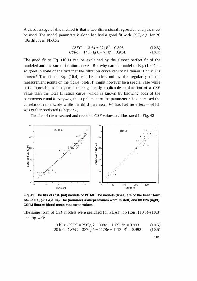
105
A disadvantage of this method is that a two-dimensional regression analysis must be used. The model parameter k alone has had a good fit with CSF, e.g. for 20 kPa drives of PDAX:
CSFC = 13.6k + 22; R2 = 0.893 (10.3) CSFC = 146.4lg k − 7; R2 = 0.914. (10.4)
The good fit of Eq. (10.1) can be explained by the almost perfect fit of the modeled and measured filtration curves. But why can the model of Eq. (10.4) be so good in spite of the fact that the filtration curve cannot be drawn if only k is known? The fit of Eq. (10.4) can be understood by the regularity of the measurement points on the (lgk,e) plots. It might however be a special case while it is impossible to imagine a more generally applicable explanation of a CSF value than the total filtration curve, which is known by knowing both of the parameters e and k. Anyway, the supplement of the parameter e has increased the correlation remarkably while the third parameter V0
e has had no effect – which was earlier predicted (Chapter 7).
The fits of the measured and modeled CSF values are illustrated in Fig. 42.
Fig. 42. The fits of CSF (ml) models of PDAX. The models (lines) are of the linear form
CSFC = a1lgk + a2e +a3. The (nominal) underpressures were 20 (left) and 80 kPa (right).
CSFM figures (dots) mean measured values.
The same form of CSF models were searched for PDAY too (Eqs. (10.5)–(10.8) and Fig. 43):
0 kPa: CSFC = 258lg k − 998e + 1169; R2 = 0.993 (10.5) 20 kPa: CSFC = 337lg k − 1178e + 1113; R2 = 0.992 (10.6)
CSFC, ml CSFC, ml
CS
F, m
l
CS
F, m
l
CSFC, ml CSFC, ml
CS
F, m
l
CS
F, m
l
CSFC, cm3CSFC, cm3
CS
FM
and
CS
FC
, c
m3
CS
FM
and
CS
FC
, cm
3
20 kPa 80 kPa
CSFC, ml CSFC, ml
CS
F, m
l
CS
F, m
l
CSFC, ml CSFC, ml
CS
F, m
l
CS
F, m
l
CSFC, cm3CSFC, cm3
CS
FM
and
CS
FC
, c
m3
CS
FM
and
CS
FC
, cm
3
CSFC, ml CSFC, ml
CS
F, m
l
CS
F, m
l
CSFC, ml CSFC, ml
CS
F, m
l
CS
F, m
l
CSFC, cm3CSFC, cm3
CS
FM
and
CS
FC
, c
m3
CS
FM
and
CS
FC
, cm
3
20 kPa 80 kPa
CSFC, ml
40 60 80 100 12040
60
80
100
120
140
CS
FM
an
dC
SF
C,
ml
CSFC, ml
40 60 80 100 12040
60
80
100
120
140
CS
FM
an
d C
SF
C,m
l
CSFC, ml CSFC, ml
CS
F, m
l
CS
F, m
l
CSFC, ml CSFC, ml
CS
F, m
l
CS
F, m
l
CSFC, cm3CSFC, cm3
CS
FM
and
CS
FC
, c
m3
CS
FM
and
CS
FC
, cm
3
20 kPa 80 kPa
CSFC, ml CSFC, ml
CS
F, m
l
CS
F, m
l
CSFC, ml CSFC, ml
CS
F, m
l
CS
F, m
l
CSFC, cm3CSFC, cm3
CS
FM
and
CS
FC
, c
m3
CS
FM
and
CS
FC
, cm
3
CSFC, ml CSFC, ml
CS
F, m
l
CS
F, m
l
CSFC, ml CSFC, ml
CS
F, m
l
CS
F, m
l
CSFC, cm3CSFC, cm3
CS
FM
and
CS
FC
, c
m3
CS
FM
and
CS
FC
, cm
3
20 kPa 80 kPa
CSFC, ml
40 60 80 100 12040
60
80
100
120
140
CS
FM
an
dC
SF
C,
ml
CSFC, ml
40 60 80 100 12040
60
80
100
120
140
CS
FM
an
d C
SF
C,m
l

106
50 kPa: CSFC = 489lg k − 1494e + 983; R2 = 0.989 (10.7) 80 kPa: CSFC = 472lg k − 1444e + 935; R2 = 0.989. (10.8)
Fig. 43. The fits of CSF models of PDAY. The models (lines) are of the linear form
CSFC = a1lgk + a2e +a3. The driving overpressures are presented on the plots. The
SGW samples are not used in the models of the two highest pressures because the
pads clearly broke. CSFM figures (dots) mean measured values.
The coefficients of the CSF models are different for the two different pieces of measurement equipment, as well as for different pressures and pulp type combinations. The signs are nevertheless the same. On the grounds of the CSF model alone we cannot however tell to what direction the freeness is changing if the value of the parameters is changed (e.g. e increased) because the parameters are not independent in practice. A certain pulping process can namely change the operation points on the (lgk, e) plot roughly only along the certain operation lines (Figs. 26 - 31) which seem to be characteristic of all pulp types (SGW, PGW, TMP and chemical pulp). These lines cross the isolines of freeness (Fig. 44). This phenomenon also limits the controllability of pulp properties (e.g. CSF) in a certain pulping process. So the model of the filtration curve and the plot of its parameters (lgk and e) can be used to illustrate the possibilities to control CSF
CSFC, cm3 CSFC, cm3
CSFC, cm3 CSFC, cm3
CS
FC
and
CS
FM
, cm
3C
SF
C a
nd C
SF
M,
cm3
CS
FC
and
CS
FM
, cm
3C
SF
C a
nd C
SF
M,
cm3
0 kPa 20 kPa
50 kPa80 kPa
CSFC, cm3 CSFC, cm3
CSFC, cm3 CSFC, cm3
CS
FC
and
CS
FM
, cm
3C
SF
C a
nd C
SF
M,
cm3
CS
FC
and
CS
FM
, cm
3C
SF
C a
nd C
SF
M,
cm3
0 kPa 20 kPa
50 kPa80 kPa
CS
FM
an
d C
SF
C, m
l
CSFC, mlCSFC, ml
CSFC, mlCSFC, ml
CS
FM
an
d C
SF
C, m
l
CS
FM
an
d C
SF
C, m
l
CS
FM
an
d C
SF
C, m
l
CSFC, cm3 CSFC, cm3
CSFC, cm3 CSFC, cm3
CS
FC
and
CS
FM
, cm
3C
SF
C a
nd C
SF
M,
cm3
CS
FC
and
CS
FM
, cm
3C
SF
C a
nd C
SF
M,
cm3
0 kPa 20 kPa
50 kPa80 kPa
CSFC, cm3 CSFC, cm3
CSFC, cm3 CSFC, cm3
CS
FC
and
CS
FM
, cm
3C
SF
C a
nd C
SF
M,
cm3
CS
FC
and
CS
FM
, cm
3C
SF
C a
nd C
SF
M,
cm3
0 kPa 20 kPa
50 kPa80 kPa
CS
FM
an
d C
SF
C, m
l
CSFC, mlCSFC, ml
CSFC, mlCSFC, ml
CS
FM
an
d C
SF
C, m
l
CS
FM
an
d C
SF
C, m
l
CS
FM
an
d C
SF
C, m
l

107
(and other pulp properties) in a certain process and to compare processes in this respect.
Fig. 44. Isolines of CSF (50 ml–600 ml) in PDAX 20 kPa (underpressure) analyses. The
dots are the (lgk,e) pairs of the filtration models.
It has been seen (Chapter 8) that the model parameters of the same pulp sample have differed greatly because the measured filtration curves produced by the (roughly made) research equipment has had poor repeatability. The modeling has however sharply separated the filtration curves of the parallel drives. The difference of the model parameters of parallel analyses is also a positive sign of the sensitivity to the changes of the filtration curve. When the model of CSF is known, the difference of the parameters of parallel analyses can be transformed to CSF units and to make it more understandable. The change of CSF due to change of e is calculated so that the value of e in the model of CSF is changed to the e value of the parallel drive, keeping the value of k the same. When calculating the effect of k, only k is changed, and when the join effect of e and k, both of them are changed. The differences of calculated CSF values between the parallel analyses caused by one of the two parameters (k or e) have typically been tens of milliliters while the joint influence on the CSF value has been only some milliliters (Table 6). This is an additional indication of the dependency of the model parameters.
ISOLINES OF CSF; 0,2 bar
50
100
300400500600
1
1,2
1,4
1,6
1,8
2
2,2
2,4
2 2,5 3 3,5 4 4,5 5 5,5
lgk
e
ISOLINES OF CSF; 0,2 bar
50
100
300400500600
1
1,2
1,4
1,6
1,8
2
2,2
2,4
2 2,5 3 3,5 4 4,5 5 5,5
lgk
e
lgk
e
ISOLINES OF CSF; 0,2 bar
50
100
300400500600
1
1,2
1,4
1,6
1,8
2
2,2
2,4
2 2,5 3 3,5 4 4,5 5 5,5
lgk
e
ISOLINES OF CSF; 0,2 bar
50
100
300400500600
1
1,2
1,4
1,6
1,8
2
2,2
2,4
2 2,5 3 3,5 4 4,5 5 5,5
lgk
e
lgk
e
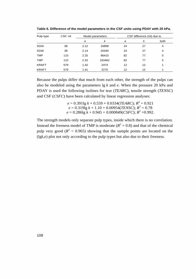
108
Table 6. Difference of the model parameters in the CSF units using PDAY with 20 kPa.
Pulp type CSF, ml Model parameters CSF difference (ml) due to
e k e k both
SGW 38 2.12 16898 24 27 4
SGW 38 2.14 20340 24 27 4
TMP 110 2.25 96415 82 77 5
TMP 110 2.32 163462 82 77 5
KRAFT 579 1.42 2474 12 12 1
KRAFT 579 1.41 2275 12 12 1
Because the pulps differ that much from each other, the strength of the pulps can also be modeled using the parameters lg k and e. When the pressure 20 kPa and PDAY is used the following isolines for tear (TEARC), tensile strength (TENSC) and CSF (CSFC) have been calculated by linear regression analyses:
e = 0.391lg k + 0.559 + 0.0334(TEARC); R2 = 0.921 e = 0.319lg k + 1.10 + 0.00954(TENSC); R2 = 0.78 e = 0.286lg k + 0.945 + 0.000849(CSFC); R2 =0.992.
The strength models only separate pulp types, inside which there is no correlation. Instead the freeness model of TMP is moderate (R2 = 0.8) and that of the chemical pulp very good (R2 = 0.965) showing that the sample points are located on the (lgk,e) plot not only according to the pulp types but also due to their freeness.

109
11 Consistency of filtrate
The consistency of the filtrate of PDAY was measured based on the transmission of polarized light. Two light beams were detected to produce “measurement signal” (M) and “reference signal” (R). The measurement signal is dependent both on the optically active particles (e.g. fibers) and total amount of particles – the reference signal only on the total amount of particles. The proportion of the two signals (M/R) indicates the consistency of fibers (in this case and more generally the consistency of birefringent material). The main purpose of this measurement was to get at least a qualitative opinion on the progress of the filtrate consistency and thereby on that of the fines retention into the fiber pad on the wire. No doubt the change of retention during the course of filtration namely affects the shape of the filtration curve – perhaps also in the modeling range of this work, which was limited between the filtrate volumes of 150 cm3 and 900 cm3.
The consistency of filtrate was determined in the laboratory for some analyses of both PDAX and PDAY. The consistency of the total filtrate of PDAX was about 0.01% – roughly 3% of the consistency of the sample to be filtrated. The increase of the driving pressure from 20 to 80 kPa increased the consistency of SGW filtrate by 14% but did not affect the TMP or PGW filtrates. The filtrate consistencies of PDAY drives were analyzed using special drives: the amount of the sample was only 250 cm3, driving pressure about 20 kPa and with no water below the screen. The filtrate consistencies of mechanical pulps (SGW and TMP) were about 0.06% and that of chemical pulp 0.02% – roughly 20 and 7% of the sample consistency. The total retention is high (about 97%) and after 250 cm3 it might (be reasoned to) be almost complete because so great a majority of the fines has passed through the wire before that (even if the retentions of PDAX and PDAY are not quite comparable).
The filtrate consistency transmitter installed for this work (LCF) in PDAY has also shown that the retention is very high and especially that its change is close to zero after the filtration of about 150 cm3 (+ 100 ml in Fig. 45, see bellow). It is the progress of retention which is of most importance to the shape of the filtration curve and slope of filtration resistance which are the main focuses of this work. Supposing that the relation of fibers and the total amount of solids remains constant, the time derivate of M/R (d(M/R)/dt) can be used to evaluate the possible effects of retention changes on the filtration curve and on its model. The amount of liquid between the screen and the LCF is about 100 cm3. So the modeling range starts from 250 cm3 in Fig. 45.

110
Fig. 45. Progress of filtrate consistency for TMP of 110 ml CSF and driving
overpressure of 20 kPa. The consistency did not change after 250 cm3 of filtrate had
passed the consistency transmitter or 150 cm3 had passed the screen.
The specific resistance of very finely ground pulps (e.g. SGW, CSF 38 ml) has been very low (Fig. 40) when the two highest filtration pressures of this work were used. This is also dramatically seen in the optical signals indicating consistency of filtrate (Fig. 46). Normally the LCF M/R signal has decreased fast (0 and 20 kPa lines) because the retention of the pad has increased but in the case of broken pad the consistency of filtrate has been high during the entire period of drainage. The 80 kPa line as a function of the filtrate volume is very noisy in the beginning as well as in the end: ultrasonic level transmitter (LT in Fig. 11) has measured splashes.
The optical signals caused by the fines in the filtrate could clearly have separated different types of pulps (Figs. 47, 48 and 50). The “fiber consistency” signal (M/R) of low freeness mechanical pulps has been highest as a function of time, which might have been caused by the high consistency and/or the slow drainage. The order has been the same as a function of filtrate volume, but the slope of SGW has been much steeper than that of TMP. The high concentration of fine material in the SGW sample was seen in the beginning of the filtration as the high consistency in the filtrate, but the retention of fines has accelerated itself and thereby decreased the volume flow rate and fines consistency of the filtrate.
PROGRESS OF FILTRATE CONSISTENCYTMP 110 ml, 0,2 bar
-0,05
-0,04
-0,03
-0,02
-0,01
0
0,01
0 200 400 600 800
V, ml
d(M
/R)/
dt
PROGRESS OF FILTRATE CONSISTENCYTMP 110 ml, 0,2 bar
-0,05
-0,04
-0,03
-0,02
-0,01
0
0,01
0 200 400 600 800
V, ml
d(M
/R)/
dt
V, cm3
d(M
/R)/
dt
PROGRESS OF FILTRATE CONSISTENCYTMP 110 ml, 0,2 bar
-0,05
-0,04
-0,03
-0,02
-0,01
0
0,01
0 200 400 600 800
V, ml
d(M
/R)/
dt
PROGRESS OF FILTRATE CONSISTENCYTMP 110 ml, 0,2 bar
-0,05
-0,04
-0,03
-0,02
-0,01
0
0,01
0 200 400 600 800
V, ml
d(M
/R)/
dt
V, cm3
d(M
/R)/
dt

111
Fig. 46. The filtrate consistency of a low-freeness pulp that is drained using too high
overpressure as a function filtrated time (left) and volume (right).
Fig. 47. The filtrate consistencies of different pulp types in non-calibrated “LCF units”
as a function of filtrated time (left) and volume (right).
The pressure has not had a big effect on the fiber consistency signals of chemical pulp or TMP (Fig. 48), but has increased fines in the filtrate of SGW pulp. The fiber consistency values have been higher for lower pressures as a function of time. Their filtrate flow rate has been however lower. That is why the order might be different as a function of the filtrate volume, which is a more illustrative plot
SGW
TMP
KRAFT
0,05
0,07
0,09
0,11
0,13
0,15
0,17
0,19
0,21
0,23
0,25
0,000 5,000 10,000 15,000
t, s
LC
F M
/R
SGW
TMP
KRAFT
0,05
0,07
0,09
0,11
0,13
0,15
0,17
0,19
0,21
0,23
0,25
0 50 100 150 200 250 300 350
V, ml
LC
F M
/R
SGW
TMP
KRAFT
0,05
0,07
0,09
0,11
0,13
0,15
0,17
0,19
0,21
0,23
0,25
0,000 5,000 10,000 15,000
t, s
LC
F M
/R
SGW
TMP
KRAFT
0,05
0,07
0,09
0,11
0,13
0,15
0,17
0,19
0,21
0,23
0,25
0 50 100 150 200 250 300 350
V, ml
LC
F M
/R
t, s V, cm3
LC
FM
/R
LC
FM
/R
SGW
TMP
KRAFT
0,05
0,07
0,09
0,11
0,13
0,15
0,17
0,19
0,21
0,23
0,25
0,000 5,000 10,000 15,000
t, s
LC
F M
/R
SGW
TMP
KRAFT
0,05
0,07
0,09
0,11
0,13
0,15
0,17
0,19
0,21
0,23
0,25
0 50 100 150 200 250 300 350
V, ml
LC
F M
/R
SGW
TMP
KRAFT
0,05
0,07
0,09
0,11
0,13
0,15
0,17
0,19
0,21
0,23
0,25
0,000 5,000 10,000 15,000
t, s
LC
F M
/R
SGW
TMP
KRAFT
0,05
0,07
0,09
0,11
0,13
0,15
0,17
0,19
0,21
0,23
0,25
0 50 100 150 200 250 300 350
V, ml
LC
F M
/R
t, s V, cm3
LC
FM
/R
LC
FM
/R
80 kPa
20 kPa
0 kPa
50 kPa
0
0,1
0,2
0,3
0,4
0,5
0,6
0,7
0,8
0 5 10 15 20 25
t, s
LC
F M
/R
0 kPa
20 kPa
50 kPa
80 kPa
0
0,1
0,2
0,3
0,4
0,5
0,6
0,7
0,8
0 200 400 600 800 1000
V, cm3L
CF
M/R
80 kPa
20 kPa
0 kPa
50 kPa
0
0,1
0,2
0,3
0,4
0,5
0,6
0,7
0,8
0 5 10 15 20 25
t, s
LC
F M
/R
0 kPa
20 kPa
50 kPa
80 kPa
0
0,1
0,2
0,3
0,4
0,5
0,6
0,7
0,8
0 200 400 600 800 1000
V, cm3L
CF
M/R
V, cm3t, s
LC
F M
/R
LC
FM
/R

112
because the area under the lines (the time integral of filtrate volume) shows the total amount of fines not arrested by the fiber pad on the wire.
Fig. 48. The effect of the pressure on the filtrate consistency signals of LCF. The four
curves of the same pulp type are driven by the four different overpressures of this
work (0, 20, 50 and 80 kPa). The lower pressure curves of the same pulp type are
higher as a function of time (left) because the filtration is slower.
The previous plots of filtrate consistencies are non-calibrated LCF signals. They are based on real optical measurements: the reference signal R represent the intensity of light transmission and (logarithm of) 1/R is proportional to the attenuation if the properties of the light source and detector are constant. The attenuation is a valid measure of turbidity, which is due to the amount, size and shape of fines in the filtrate. The measurement signal of LCF (M) is proportional to the amount of light the polarization vector direction of which is turned. The more fibers in the filtrate the more “turned” light but of course it is also damped by the fines before the detector; the effect of damping can be compensated by using the R signal: M/R describes the fiber concentration of the filtrate and total fines concentration if the relation of the fibers and the rest of the fines is constant. This condition makes the calibration questionable. The properties of solids in the filtrate are surely different from those in the sample. The filtration changes them – probably also during the course of the filtration so that the fines distributions are quite different in the beginning and in the end of an individual drainage. So the transformation equations from the M/R signal to the consistency percent should be changed during the course of the analyzer drive. This is impossible.
SGW
TMP
KRAFT0,055
0,075
0,095
0,115
0,135
0,155
0,175
0,195
0,215
0,235
0,255
3 4 5 6 7 8 9 10
t , s
LC
F M
/R
SGW
TMP
KRAFT
0,055
0,075
0,095
0,115
0,135
0,155
0,175
0,195
0,215
0,235
0,255
0 100 200 300 400 500
V , cm3
LC
F M
/R
SGW
TMP
KRAFT0,055
0,075
0,095
0,115
0,135
0,155
0,175
0,195
0,215
0,235
0,255
3 4 5 6 7 8 9 10
t , s
LC
F M
/R
SGW
TMP
KRAFT
0,055
0,075
0,095
0,115
0,135
0,155
0,175
0,195
0,215
0,235
0,255
0 100 200 300 400 500
V , cm3
LC
F M
/R

113
The calibration was done so that samples of 250 cm3 were filtrated using the pressure of 20 kPa without water below the wire. The consistency of the filtrate was analyzed in the laboratory. The filtrate was diluted by water and poured through LCF; this was repeated several times to get the measurement points seen in Fig. 49. The connection between M/R values and measured consistency was linear and the correlation was high (Fig. 49):
KRAFT: C = 0.730(M/R) −0.0492; R2 = 0.998 (11.1) TMP: C = 0.863(M/R) −0.0588; R2 = 0.998 (11.2) SGW: C = 0.634(M/R) −0.0446; R2 = 0.996 (11.3)
Fig. 49. The calibration of LCF signals. Filtrates of 250 cm3 are gradually diluted by
water and measured by LCF. The (nominal) overpressure of 20 kPa is used to produce
the first sample.
The fiber concentration (M/R) related to the total consistency is different for different types of pulps and so are the calibration lines, too. Normally (for non-filtrated pulps) the slope of the line of the chemical pulp is about twice as large as that of the mechanical pulp because the latter contains more non-fibrous solids. The calibration line of chemical pulp filtrate is however between the lines of SGW and TMP. The filtration seems to turn the lines or the portions of fibrous material closer to each other.
In spite of the fact that the calibration is done by adding water, not by decreasing solids by filtration it is used to transform the M/R curves (Fig. 47) to consistency curves (Fig. 50). TMP increases closer to SGW and farther from chemical pulp, which comes closer to SGW. Pulp types are still separating clearly as a function of both time and the filtrate volume. These (calibrated) consistencies
SGW
TMP
KRAFT
0
0,01
0,02
0,03
0,04
0,05
0,06
0,07
0,07 0,09 0,11 0,13 0,15 0,17
LCF M/R
CO
NS
IST
EN
CY
, %
TMP
SGW
KRAFT
0
0,01
0,02
0,03
0,04
0,05
0,06
0,07
0,2 0,25 0,3 0,35 0,4 0,45 0,5 0,55LCF 1/R
CO
NS
IST
EN
CY
, %SGW
TMP
KRAFT
0
0,01
0,02
0,03
0,04
0,05
0,06
0,07
0,07 0,09 0,11 0,13 0,15 0,17
LCF M/R
CO
NS
IST
EN
CY
, %
TMP
SGW
KRAFT
0
0,01
0,02
0,03
0,04
0,05
0,06
0,07
0,2 0,25 0,3 0,35 0,4 0,45 0,5 0,55LCF 1/R
CO
NS
IST
EN
CY
, %
LFC M/R LFC M/R
SGW
TMP
KRAFT
0
0,01
0,02
0,03
0,04
0,05
0,06
0,07
0,07 0,09 0,11 0,13 0,15 0,17
LCF M/R
CO
NS
IST
EN
CY
, %
TMP
SGW
KRAFT
0
0,01
0,02
0,03
0,04
0,05
0,06
0,07
0,2 0,25 0,3 0,35 0,4 0,45 0,5 0,55LCF 1/R
CO
NS
IST
EN
CY
, %SGW
TMP
KRAFT
0
0,01
0,02
0,03
0,04
0,05
0,06
0,07
0,07 0,09 0,11 0,13 0,15 0,17
LCF M/R
CO
NS
IST
EN
CY
, %
TMP
SGW
KRAFT
0
0,01
0,02
0,03
0,04
0,05
0,06
0,07
0,2 0,25 0,3 0,35 0,4 0,45 0,5 0,55LCF 1/R
CO
NS
IST
EN
CY
, %
LFC M/R LFC M/R
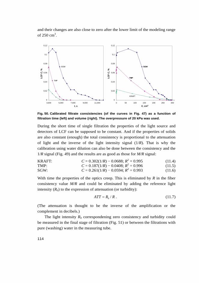
114
and their changes are also close to zero after the lower limit of the modeling range of 250 cm3.
Fig. 50. Calibrated filtrate consistencies (of the curves in Fig. 47) as a function of
filtration time (left) and volume (right). The overpressure of 20 kPa was used.
During the short time of single filtration the properties of the light source and detectors of LCF can be supposed to be constant. And if the properties of solids are also constant (enough) the total consistency is proportional to the attenuation of light and the inverse of the light intensity signal (1/R). That is why the calibration using water dilution can also be done between the consistency and the 1/R signal (Fig. 49) and the results are as good as those for M/R signal:
KRAFT: C = 0.302(1/R) − 0.0688; R2 = 0.995 (11.4) TMP: C = 0.187(1/R) − 0.0408; R2 = 0.996 (11.5) SGW: C = 0.261(1/R) − 0.0594; R2 = 0.993 (11.6)
With time the properties of the optics creep. This is eliminated by R in the fiber consistency value M/R and could be eliminated by adding the reference light intensity (R0) to the expression of attenuation (or turbidity):
0 /ATT R R . (11.7)
(The attenuation is thought to be the inverse of the amplification or the complement in decibels.)
The light intensity R0 correspondening zero consistency and turbidity could be measured in the final stage of filtration (Fig. 51) or between the filtrations with pure (washing) water in the measuring tube.
SGWSGW
TMPTMP
KRAFT
0
0,02
0,04
0,06
0,08
0,1
0,12
0 50 100 150 200 250 300
V, mlL
CF
C, %
SGW
TMP
0
0,02
0,04
0,06
0,08
0,1
0,12
3,000 5,000 7,000 9,000 11,000
t, s
LC
F C
, %
SGWSGW
TMPTMP
KRAFT
0
0,02
0,04
0,06
0,08
0,1
0,12
0 50 100 150 200 250 300
V, mlL
CF
C, %
SGW
TMP
0
0,02
0,04
0,06
0,08
0,1
0,12
3,000 5,000 7,000 9,000 11,000
t, s
LC
F C
, %
t, s V, cm3
LC
F C
,%
LC
F C
,%
SGWSGW
TMPTMP
KRAFT
0
0,02
0,04
0,06
0,08
0,1
0,12
0 50 100 150 200 250 300
V, mlL
CF
C, %
SGW
TMP
0
0,02
0,04
0,06
0,08
0,1
0,12
3,000 5,000 7,000 9,000 11,000
t, s
LC
F C
, %
SGWSGW
TMPTMP
KRAFT
0
0,02
0,04
0,06
0,08
0,1
0,12
0 50 100 150 200 250 300
V, mlL
CF
C, %
SGW
TMP
0
0,02
0,04
0,06
0,08
0,1
0,12
3,000 5,000 7,000 9,000 11,000
t, s
LC
F C
, %
t, s V, cm3
LC
F C
,%
LC
F C
,%

115
Fig. 51. The possible measurement point for the reference value of the consistency
intensity, R0.
The water dilution calibration is not valid for a filtration dilution especially for M/R because the properties of solids are changing during the course of the drainage. This phenomenon might be used to characterize the drainage properties of different kinds of pulps. The mutual progression of the two LCF signals 1/R (proportional to the turbidity) and M/R (proportional to the fiber consistency) can be plotted in the same coordinates (Fig. 52).
R0
AIR
2
2,5
3
3,5
4
4,5
5
5,5
0 10 20 30 40 50 60 70 80
t , s
LC
F R
R0R0
AIR
2
2,5
3
3,5
4
4,5
5
5,5
0 10 20 30 40 50 60 70 80
t , s
LC
F R
R0

116
Fig. 52. The values of LCF transmitter during the course of the water dilution and the
filtration dilution. In the case of calibration (CALIBR) the sample is diluted using water.
The rest of the curves (TMP, SGW and KRAFT) are measured during normal filtration
using the overpressure of 20 kPa.
The special case of Fig. 52 shows interesting differences between pulp types. E.g., simply the difference of maximum fiber consistencies and turbidity might be informative. There are differences in the turbidity on the same fiber consistency level. One can also see that filtration curves are steeper than water dilution curves showing that the fiber retention has dominated; the curve of chemical pulp is almost upright which means that the fiber consistency is changed much while the turbidity is hardly changed at all.
TMP
SGW
0,05
0,07
0,09
0,11
0,13
0,15
0,17
0,19
0,21
0,23
0,25
0,2 0,3 0,4 0,5 0,6 0,7
LCF 1/R
LC
F M
/R
TMP CALIBR
SGW CALIBR
KRAFT CALIBR
TMP
SGW
KRAFT
LCF 1/R
LC
F M
/R
TMP
SGW
0,05
0,07
0,09
0,11
0,13
0,15
0,17
0,19
0,21
0,23
0,25
0,2 0,3 0,4 0,5 0,6 0,7
LCF 1/R
LC
F M
/R
TMP CALIBR
SGW CALIBR
KRAFT CALIBR
TMP
SGW
KRAFT
LCF 1/R
LC
F M
/R

117
12 Discussion
The separation of pulp suspensions into solids and liquids, e.g. the filtration or drainage or dewatering are the key operations of the papermaking process. That is why it is important to know the filtration properties of the pulp to be processed. Many kinds of analyzers are used to measure different quantities to describe these. The main target of this work has been to develop mathematical models to describe the course of the filtration curves. On the other hand, by measuring the many basic phenomena happening in the filtration (analyzers) it can be supposed that information can be found not only about dewaterability itself but also about other important properties of pulp and the final product (e.g. paper) made of it as well as about the states of dewatering and other papermaking processes.
Filtrations are complicated operations in papermaking processes and are as complicated as the raw materials involved, like pulp suspensions and slurries. One single figure has surprisingly dominated the description of this multidimensional phenomenon. The filtration curves carry much more information and by using the model of this work it can be packed into one figure pair – not too much more than one (CSF) figure. The noise filtering effect of the modeling has made the filtration curves more clear and informative. In the past, the papermakers were not able to use multidimensional information and perhaps the most important and also the most commonly used single quality factor of the pulps has been and probably will be in the near future the very freeness figure: “pulp of 120 ml” or just “the number of is 120” is the deep-seated way of thinking – and for weighty reasons. Today trends and profiles of many kinds of quantities are used to control various papermaking processes. So all the professionals (from designers of the papermaking processes to the salesmen of the paper products) connected to papermaking are also ready to exploit the additional information given by the filtration curves – surely not to displace CSF or SR figures but to supplement them.
It is out of the scope of this work to scientifically evaluate the possible benefits of this additional process information. The freeness value is however used for direct control of grinders and refiners and is of a most basic knowledge when driving the former and thereby the very complicated multivariable wet end system of many feedbacks and other interactions. These processes govern both the quality of pulp and the energy consumption of the papermaking process. This is based on a single freeness figure and on the at least mental opinion of darcy-like behavior of the pulp outside this single freeness point. It has however been

118
seen in this work that the real values of filtrating quantities (e.g. filtration rate and specific resistance) may be many percents different from this assumption: they change remarkably during the course of the drainage and due to the change of the filtrating pressure. If only a couple of points of the filtration curve are measured, the noise may make the results totally meaningless, especially in the starting and finishing state of filtration. In addition the process may amplify the effect of the false information about dewaterability: e.g. if a grinder (of 5 MW!) is controlled according to a too high assumption about the true dewaterability, more energy is wasted to compensate for it and pulp of too slow dewaterability is produced; this means too slow filtration in the former and more energy must be wasted to evaporate the moisture out of wet web or the rate of production must be decreased; and perhaps the web is broken – very expensive consequences.
Papermaking is a business of a most mature technology and market as well as of great volume of production. So the quality limits are unconditional and the marginal of the (e.g. energy) cost narrow. This is to say that small improvements to the technology might be of vital importance. The knowledge of the dewaterability is so valuable that if one can completely exploit a drainage analyzer that reduces the error of total drainability by many percent, payback time cannot be more than a couple of months and even the total competitivity of the mill can increase remarkably due to the narrow limits of possible costs and quality.
So all the papermakers are forced on taking into account e.g. the following observations: the filtration phenomenon is multidimensional and cannot be described by one figure, the filtration curve is not “darcy-like”; the specific filtration resistance is not constant during the filtration and it is dependent on the pressure; the random noise of the basic measurement of filtration might totally mask the measurement information; the consistency and portion of the fibrous fines is changing, etc. This work may help the papermakers to overcome these difficulties.
The controllability of any process quantity is limited by the quality of the measurements which the control is based on. Many of the results of this thesis might be used to improve the measurement of the drainability of pulps. The very first link of the measurement chain in an analyzer is in many cases the most crucial point for the quality of the measurement. There cannot be any built-in correcting feedback and errors of the first link are fed through all the analyzers and usually amplified on the way. That is why one must pay attention and invest in the sample conditioning of the drainage analyzer and a conditioner of the sample volume, temperature and consistency is a self-evident accessory. Even the
119
rough prototype of this work has met the need, but careful finishing of the product design will surely pay for itself.
The correlation coefficient of the CSF model based on our filtration model is clearly better than that of a typical fit between CSF values of commercial process analyzers and laboratory testers. Due to our rough methods employed to produce the modeled filtration curves, their repeatabilities were poor, but the model was as good for all the curves made from the same sample and the model followed exactly all of them separating them clearly from each other. The amount of filtrate is not linear as a function of time – nor can its basic model be. Our model can be linearized using logarithms of the quantities after getting the two main parameters and ignoring the one that is meaningless in this phase. The direct fit of the logarithmic models using linear regression analysis cannot be recommended because in the very beginning of the filtration the dominating phenomena are observed to be fast, noisy and different from the rest of the filtration.
The filtration curve can be easily and exactly measured and stored into two figures. Instead of measuring a couple of filtration curve points for calculating the CSF output of their analyzers, the companies that are planning, making, selling and installing drainage meters and control systems based on the measurements, should offer equipment and control algorithms that utilize the additional information from the filtration curves. Even the CSF figure is useful to be calculated using the two model parameters of the filtration curve. The model is also a very effective filter of random noise and could be used to replace or supplement the normal RC filters of drainage transmitters. The effective noise filtering naturally reduces the pressure on the quality and expenses of the sensor hardware.
Without the idea of the temporary model parameter, the timing of the start of filtration should be very exact due to the fast phenomena in the very beginning. Expensive precision technology would be necessary while the filtration of the system using our model may be started any time. The curve is not modeled from the very beginning of the filtration but in many cases it might be useful to extrapolate it to the origin as an estimate of the (potential) filtration curve; as additional information could be used, e.g. the consistency of the filtrate and the resistance of the screen instead of the noisy measurement of the filtrated volume. It is much easier to hit the modeled than the measured curve on the origin.
Or perhaps the continuously measured optical properties of the filtrate are better quantities to describe the beginning of drainage than the filtration curve. The fines consistency of the filtrate was clearly different for different pulp types
120
and decreased quickly. Also the portion of the optically active fines changed and this separation could be supposed to continue inside the pad, surely affecting many important properties of the wet web and paper. More careful measuring of this phenomenon should be most informative.
The status of the specific filtration resistance as a quality factor of the pulp could be higher. When the driving pressure is measured and the two model parameters known, the resistance can be easily calculated using the equations derived in this work. It has been seen that the response of the driving pressure on the specific resistance differs outstandingly from one pulp type to another. So the drainage analyses using different pressures give useful information and it is most advisable to include this possibility also in commercial analyzers. The multipressure drives together with the models of the filtration and resistance curves make it possible to simulate the shapes of the filtration curves produced by different kinds of driving pressures, which are not used in the real analyses: at least the responses of the constant, step and impulse pressures must be interesting. The producing of constant filtration pressure is a demanding task and it might be better to calculate the constant-pressure filtration volume curves as well as the pressure curves of the constant filtration rate analyses. The means of this sort of transformations are however not systematically studied in this work but hopefully will be done in the upcoming examinations.
Plenty of information about pulp and its processing into paper and other products can already be obtained by measuring the filtration of pulp samples in different kinds of analyzers. The phenomenon field during the filtration of the pulp is however so rich that it can be supposed that the great majority of the scientifically, technically and commercially interesting and valuable knowledge is still hidden. More and more of it can and must be dug up using invariably developing measurement technology. Experimental exactly controllable filtration system(s) should be built and encircled by all possible available up-to-date measurement systems to continuously measure, e.g., the movements and the properties of the (especially tiny) particles of the sample, pad and filtrate, the development of the thickness, surface and voids of the pad, air transmission, etc. In addition to the traditional instruments one could utilize advanced ultrasonic and optical methods like polarization, reflection coefficient, photoacoustic, scattering, time of flight, and image processing measurements. The capture of all possible information relating to pulp drainage is worthy of a forceful research program or maybe even of a permanent research group.

121
13 Summary
The main goal of this thesis was to develop an empirical mathematical model of filtration curve as a component of pulp drainage analyzers.
Filtration is usually assumed to follow the so called Darcy’s law: the filtrated volume is proportional to the square root of the filtration time or in the other words the time to filtrate a certain volume is proportional to the square of the filtrated volume. In this work it has been seen that this happens only in a special case and in most cases the filtration curve is more or less curvy than Darcy’s law suggests. Happily, it turned out that the models of the curves are of the same mathematical form as that of Darcy’s law – just the exponent of the filtrated time or volume is different. This means that the equation of Darcy’s law is a special case of our equation and makes it easy to see and calculate how “darcy-like” the pulp and the filtration are.
It was seen that the model is not valid in the very beginning of the filtration due to, e.g. the effect of the screen and of the change of the fines retention into the pad. The latter was detected by installing an optical transmitter to measure the consistency of filtrate during the course of filtration. So the modeling cannot start from the origin. To overcome this problem an auxiliary parameter was added to the model. It is used only during the modeling calculations and can be ignored as soon as one has obtained the two more parameters that describe the filtration properties of the pulp itself. The parameters can be obtained using an easily available linear regression analysis program. The fit between the used empirical model and the measurements has been so good that the correlation coefficient has typically been about 0.9999 for a wide range of pulps and driving pressures using both under- and overpressures. The points of different pulp types were logically located on the coordination of the two parameters.
Like all the measurements, also the drainage curve includes random noise and all the analyzers must have means to filter it out. In this case a simple RC-filter or moving averaging cannot be used because they would destroy the shape of the curve. The disturbances of the calculated specific resistances were shown to increase dramatically towards the end of the filtration especially when using low pressures. Our model worked very well also as a filter of random noise.
The parameters could be modeled to calculate freeness (CSF) values of a wide range of pulp types. The CSF-models based on the parameters of our filtration curve were better than any model based on the individual pairs of filtration time and volume.
122
The temperature and consistency of the sample strongly affects the result of any freeness analyzer and the effect is dependent on the pulp types. Correction tables and mathematical models are necessary to be used because these quantities usually differ from the nominal values. This kind of correction cannot be exact especially when the difference is big and the pulp type unknown (e.g. a mix of many pulp types). Naturally the amount of the sample must also be constant. In this work a simple conditioner was constructed to show that it is able to simultaneously control the volume, temperature and consistency of the pulp sample so constantly that the total error caused by the difference from their nominal values is less than one percent on the CSF freeness value of 100 ml (or cm3). Mathematical expressions were also derived to calculate the combinations of the sample volume, temperature and consistency, which are able to be controlled to their nominal values.
The driving pressure of the filtration was carried out by an air container. The pressure decreased during the course of the filtration. It was however measured and taken into account when calculating the course of the specific filtration resistance using the mathematical expressions based on our filtration models. The level of the pressure affected both the resistance and its change during the course of the drainage. These effects were different on different pulp types. According to Darcy’s law the specific resistance should have been constant during the filtration. By comparing the resistance curves produced by different pressures, it was shown that the decreasing trend of the driving pressure has not caused the “non-darcy-like” shapes of the filtration curves.
The filtrate flow below the screen was measured by an optical transmitter. It showed that the fines consistency was different for different types of pulps, decreased rapidly close to zero and that the portion of the optically active fines did not remain constant. The main result of this measurement was that the retention was high and constant enough in the modeling range of the filtrated volume.

123
References
Aaltonen P (1983a) Sulpun suotautuminen. Paperin valmistus, Suomen Paperi-insinöörien yhdistyksen oppi- ja käsikirja III, Osa 1, Turku: 121–149.
Aaltonen P (1983b) Paperirainan tiivistyminen. Paperin valmistus, Suomen Paperi-insinöörien yhdistyksen oppi- ja käsikirja III, Osa 1, Turku: 151–168.
von Alfthan G (1962) An apparatus for continuous recording of the drainage properties of groundwood pulp. Paperi ja Puu 44(4a): 241–248.
Biermann CJ (1996) Handbook of Pulping and Papermaking. San Diego, Academic Press Inc.
Brewster DB & Rogers JH (1985) Analysis of on-line pulp drainage testers. Pulp & paper Canada 86(7): 30–34.
Brewster DB & Trepanier RJ (1999) Intelligent Drainage Analysis. TAPPI Engineering and Process & Product Quality Control Conference, Anaheim, Sept. 1999, TAPPI Proceedings: 1205–1214.
Brit KW, Unbehend JE & Holman JC (1982) Dynamic drainage of paper stock. Tappi Journal 65(11): 64–66.
Cambell WB (1947) The Physics of Water Removal. Pulp and Paper Magazine of Canada 48(3): 103–109, 122.
Cole CA, Hubbe MA & Heitmann JA (2008) Water release from fractionated stock suspensions. Part 1 – Effects of the amounts and types of fiber fines. Tappi Journal 7(7): 28–32.
Clark Jd’A (1985) Pulp Technology and Treatment for Paper. 2nd edition, San Francisco, Miller Freeman Publications Inc.
Csordas E & Schiel C (1978) Predicting drainage performance during web formation. Pulp & Paper Canada 79(11): 79–82.
Darcy H (1856) Fontaines publiques de la ville de Dijon. English.Dubuque, Iowa, Kendall/Hunt Pub. Co., 2004.
Ebeling K (1983) Puukuidun vesisorptio ja turpoaminen. In: Arjas A (ed) Paperin valmistus. Turku, Suomen paperi-insinöörien yhdistys ry: 47–66.
El-Hosseiny F & Yan JF (1980) Analysis of Canadian Standard Freeness. Pulp & Paper Canada 81(6): T113-T118.
Forsberg S & Bengtsson M (1990) The Dynamic Drainage Analyser (DDA). Proc Papermakers Conference. Atlanta, GA, USA: 239–245.
Gullichsen J (2000) Fiber line operations. In: Gullichsen J & Fogelholm C-J (eds) Papermaking Science and Technology 6. Chemical pulping. Helsinki, Fapet Oy: A17-A243.
Hiltunen E (1999) Papermaking properties of pulp. In: Gullichsen J, Paulapuro H, Levlin J-E & Söderhjelm L (eds) Papermaking Science and Technology 17. Pulp and paper testing. Helsinki Fapet Oy: 38–63.
Hubbe MA, Heitmann JA, Cole CA (2008) Water release from fractionated stock suspensions. Part 2. Effects of consistency, flocculants, shear, and order of mixing. Tappi Journal 7(8): 14–19.

124
Ingmanson WL (1952) An Investigation of the Mechanism of Water Removal from Pulp Slurries. Tappi 35(10): 439–448.
Ingmanson WL (1954) The Filtration Resistance of Pulp Slurries. Pulp and Paper Magazine of Canada 55(December):121–131.
Ingmanson WL (1964) Filtration of high consistency fiber suspensions. Tappi 47(12): 742–750.
Kajaani, Kajaani Pulp Expert, Your pulp quality fingerprint, Metso Automation 8/2008. Karrila S, Räisänen K & Paulapuro H (1992) The Moving Belt Drainage Tester. Proc
Papermakers Conference. Nashville, TN, USA: 275–299. Koskinen K (2000) Wood handling applications. In: Gullichsen J & Fogelholm C-J (eds)
Papermaking Science and Technology 6. Chemical pulping. Helsinki, Fapet Oy: A328-A491.
Lindholm C-A (1999) Bleaching. In: Gullichsen J, Paulapuro H & Sundholm J (eds) Papermaking Science and Technology 5. Mechanical Pulping. Helsinki, Fapet Oy: 311–343.
Lorentzen & Wettre, L&W Pulp Tester, Online system for standardized pulp testing, CODE 960
Lumiainen J (2000) Refining of chemical pulp. In: Paulapuro H (ed) Papermaking Science and Technology 8. Papermaking. Part 1, stock preparation and wet end. Helsinki, Fapet Oy: 86–122.
Marttinen J (1986) Suspensionsanalys av olika fibermassor med SUSAN, en typ av freeness-konsistensmetare. MSc (Eng) thesis, Åbo Akademi, Kemisk-tekniska fakultet.
Mutek, The Dynamic Drainage Analyser manual. Version 3xx, December 2001. Niskanen K, Kajanto I & Pakarinen P (1998) Paper structure. In: Gullichsen J, Paulapuro
H, Niskanen K (eds) Papermaking science and technology 4. Paper Physics. Helsinki, Fapet Oy: 13–53.
Norell M, Johansson K & Persson M (1999) Retention and drainage. In Gullichsen J, Paulapuro H & Neimo L (eds) Papermaking Science and Technology 4. Papermaking chemistry. Helsinki, Fapet Oy: 42–81.
Norman B (2000) Web forming. In: Paulapuro H (eds) Papermaking science and technology 8. Papermaking. Part 1, stock preparation and wet end. Helsinki, Fapet Oy: 191–250.
Olsson B, On-line de-watering measurement - a new parameter for wet-end control. Paper Technology 42(10): 41–45.
Page D, Barbe M, Seth R & Jordan B (1984) The mechanism of curl creation, removal and retention in pulp fibers. Journal of Pulp and Paper Science 10(3): J74–J79.
Parker JD (1972) The Sheet-Forming Process. Atlanta, GA, Technical Association of Pulp and Paper Industry.
Pradis MA, Genco JM, Bousfield DW, Hassler JC & Wildfong V (2003) Measurement of Drainage under Conditions of Known Shear Rate. Journal of Pulp and Paper Science 29(12): 395–400.

125
Pikka O, Vesala R, Vilpponen A, Dahllof H, Germgard U, Noren S, Bokstrom M, Steffes F & Gullichsen J (2000) Bleaching applications. In: Gullichsen J & Fogelholm C-J (eds) Papermaking Science and Technology 6. Chemical pulping. Helsinki , Fapet Oy: A616-A665.
Sampson WW & Kropholler HW (1995) Batch-drainage curves for pulp characterizaion. Tappi Journal 78(12): 145–151.
Sampson WW & Kropholler HW (1996) Batch-drainage curves for pulp characterizaion. Tappi Journal 79(1): 151–160.
Seppälä MJ (ed), Klemetti U, Kortelainen V-A, Lyytikäinen J, Siitonen H, Sironen R (2001) Kemiallinen metsäteollisuus I, Paperimassan valmistus. Jyväskylä, Gummerus Kirjapaino Oy.
Sundholm J (1999) What is mechanical pulping. In: Gullichsen J, Paulapuro H & Sundholm J (eds) Papermaking Science and Technology 5. Mechanical Pulping. Helsinki, Fapet Oy: 16–21.
Swodzinski PC & Doshi MR (1986) Mathematical models of Canadian Standard Freeness (CSF) and Schopper-Riegler Freeness (SR). TAPPI International process and materials quality evaluation conference. Atlanta, GA, USA: 21–24.
TAPPI (1997) Interconversion of freeness. Pulping and Paper Products, 97/98 Technical Information papers. Atlanta, GA, USA, TAPPI Press: TIP 0809–01.
TAPPI (2004) Freeness of pulp (Canadian standard method). TAPPI Test Methods. Atlanta, GA, USA, Tappi Press: T 227 om-99.
Wahlström B & O’Blenes G (1962) The Drainage of Pulps at Paper-Making Rates and Consistencies Using a New Drainage Tester. Pulp and Paper Magazine of Canada. 63(August):T-405-T-417.
Wider HD (1960) The Compression Creep Properties of Wet Pulp Mats. Tappi 43(8): 715–720.
Wildfong VJ, Genco JM, Shands JA & Bousfield DW (2000a) Filtration Mechanics of Sheet Forming. Part I: Apparatus for Determination of Constant-Pressure Filtration Resistance. Journal of Pulp and Paper Science 26(7): 250–254.
Wildfong VJ, Genco JM, Shands JA & Bousfield DW (2000b) Filtration Mechanics of Sheet Forming. Part II: Influence of Fine Material and Compression. Journal of Pulp and Paper Science 26(8): 280–283.
Wildfong VJ, Shands JA, Bousfield DW & Genco JM (2001a) Drainage during roll forming: model validation using pilot papermachine data (2001) Tappi Journal 84(7):56.
Wildfong VJ, Shands JA, Bousfield DW & Genco JM (2001b) Drainage during roll forming - model validation using pilot papermachine data (2001) Tappi Journal Peer Reviewed Paper 84(7): 1–14.

126

127
Appendix 1 Derivation of the conditioning model of consistency
After the target mass (mt) of the sample has been reached and the overflow has started and the overflow equals to the mass flow rate of dilution water (qm) in the container. During a differential time period (dt) the consistency all over the container and in the overflow is C = mk/mt and the change of solid material (mk) is:
kk
t
d d dm mmm q C t q tm
.
By separating the variables
=> k
k t
d 1d dmqm t tm m
, where t
m
mq
and by integrating both sides of the equation
=> k 1ln tm I
, where I1 is a constant
=> 1k
t Im e
=> 1 1
k 2
t t t t
t I I ttm I ee e eCm m m m
, where I2 is a constant.
In the beginning of the constant volume phase of conditioning t = t1 and C = C1. After substituting these to the previous equation the constant I2 can be solved:
=> 1
21
t
tI eCm
=> 12 1 t
tI C m e
So at the moment t (≥ t1) the consistency in the conditioner is
1
11 t1
t
t tt tC m e eC C e
m

128
Appendix 2 Derivation of the conditioning model of temperature
During the constant volume or overflow phase the energy balance must be calculated over a short period dt. During this time the water running into the container is qmdt and its temperature changes from TV to the sample temperature of the moment (to T) while the water takes the energy from the heating power P and from the temperature change of the sample (dT):
V h h t( ) d d dmT T c q T P t c m T .
By separating the variables:
h t
h V h
d dm m
c mt TP c q T c q T
.
By integrating from the beginning of the overflow (t1,T1) to the moment (t,T):
1 1
h t
h V h
d dt T
m mt T
c mt TP c q T c q T
The following integration rule can be applied:
d ln .
f xx f x I
f x
In this case f(x) > 0 and I may be ignored, because the integral is defined:
1 1
t h
h V h
d dt T
m
m m mt T
m c qt Tq P c q T c q T
=> t1 h V h h V h 1ln lnm m m m
m
mt t P c q T c q T P c q T c q Tq
=> h V h1
t h V h 1
ln m m
m m m
P c q T c q Tt tm q P c q T c q T
=> 1
t h V h
h V h 1
e m
t tm q m m
m m
P c q T c q TP c q T c q T
=> 1
th V h 1 h V
h h
e m
t tm qm m m
m m
P c q T c q T P c q TTc q c q

129
=> 1
tV 1 V
h h
m
t tm q
m m
P PT T T e Tc q c q
By substituting the time constant of the conditioner τ = mt /qm, T∞ = P/(chqm) + TV and the final temperature (T1) of the growth phase of the conditioning from Eq. (6.10):
1
0 0V V 0 V
h t h t
1 et t
m m
m mP PT T T T T Tc q m c q m
=> 1
0 0 00 V
h t t h h t
et t
m m m
m m mP P PT T T Tc q m m c q c q m
=> 1
00 V
t h
et t
m
m PT T T Tm c q
=> 1
e1et t
T T T
,
where 01 0 V
t he
m
m PT T Tm c q
.

130
Appendix 3 Schematic illustration of the consistency measurement
This measurement principle is based on the optical activity of fibrous material of the pulp. Polarized light is fed through the sample and the polarization vector is turned by the fibrous material. This portion of the light is filtered to a detector by a polarized filter and the non-turned portion to another detector. So two basic measurement signals (M and R) are produced.
This measurement principle is user, e.g. Kajaani LC-100 transmitter, that is tailored for this work to measure the consistency of the sample conditioner (LCX) and the fines of content of the filtrate (LCF).
LIG
HT
SO
UR
CE
OP
TIC
S
PO
LAR
IZE
D F
ILT
ER
ME
AS
UR
EM
EN
T C
ELL
BEAM SPLITTER
DE
TE
CT
OR
LIG
HT
SO
UR
CE
OP
TIC
S
PO
LAR
IZE
D F
ILT
ER
ME
AS
UR
EM
EN
T C
ELL
BEAM SPLITTER
DE
TE
CT
OR

131
Appendix 4 Filtration curves
Dots are measurements, lines represent models of those. h = V/A, where V is filtrated volume and A the area of the screen. The figures after pulp types are CSF values.
Fig. 4.1 PDAX, underpressure 20 kPa.
Fig. 4.2 PDAX, underpressure 80 kPa.
SGW 57
TMP 126 PGW102
0
100
200
300
400
500
600
700
800
900
1000
0 10 20 30 40 50
t , s
V, m
l
0
2
4
6
8
10
h, cm
TMP 126 PGW 102
SGW 57
0
100
200
300
400
500
600
700
800
900
1000
0 10 20 30 40 50 60 70
t , s
V, m
l
0
2
4
6
8
10
h, cm

132
Fig. 4.3 PDAY, pressure 0 kPa.
Fig. 4.4 PDAY, overpressure 20 kPa.
SGW 38
TMP124KRAFT 472
0
100
200
300
400
500
600
700
800
900
1000
0,0 20,0 40,0 60,0 80,0 100,0 120,0 140,0
t , s
V, m
l
0
2
4
6
8
10
12
h, cm
SGW 38
TMP 124KRAFT 472
0
100
200
300
400
500
600
700
800
900
1000
0,0 20,0 40,0 60,0 80,0 100,0 120,0
t , s
V, m
l
0
2
4
6
8
10
12
h,
cm

133
Fig. 4.5 PDAY, overpressure 50 kPa.
Fig. 4.6 PDAY, overpressure 80 kPa.
SGW 38
TMP 124
KRAFT 472
0
100
200
300
400
500
600
700
800
900
1000
0,0 5,0 10,0 15,0 20,0 25,0 30,0 35,0
t , s
V, m
l
0
2
4
6
8
10
12
h, cm
SGW
38
TMP 124
KR
AFT 4
72
0
100
200
300
400
500
600
700
800
900
1000
0 5 10 15 20 25 30
t , s
V,
ml
0
2
4
6
8
10
12
h, cm

134

A C T A U N I V E R S I T A T I S O U L U E N S I S
Book orders:Granum: Virtual book storehttp://granum.uta.fi/granum/
S E R I E S C T E C H N I C A
363. Isokangas, Ari (2010) Analysis and management of wood room
364. Väänänen, Mirja (2010) Communication in high technology product developmentprojects : project personnel’s viewpoint for improvement
365. Korhonen, Esa (2010) On-chip testing of A/D and D/A converters : static linearitytesting without statistically known stimulus
366. Palukuru, Vamsi Krishna (2010) Electrically tunable microwave devices using BST-LTCC thick films
367. Saarenpää, Ensio (2010) Rakentamisen hyvä laatu : rakentamisen hyvän laaduntoteutuminen Suomen rakentamismääräyksissä
368. Vartiainen, Johanna (2010) Concentrated signal extraction using consecutivemean excision algorithms
369. Nousiainen, Olli (2010) Characterization of second-level lead-free BGAinterconnections in thermomechanically loaded LTCC/PWB assemblies
370. Taskila, Sanna (2010) Improved enrichment cultivation of selected food-contaminating bacteria
371. Haapala, Antti (2010) Paper machine white water treatment in channel flow :integration of passive deaeration and selective flotation
372. Plekh, Maxim (2010) Ferroelectric performance for nanometer scaled devices
373. Lee, Young-Dong (2010) Wireless vital signs monitoring system for ubiquitoushealthcare with practical tests and reliability analysis
374. Sillanpää, Ilkka (2010) Supply chain performance measurement in themanufacturing industry : a single case study research to develop a supply chainperformance measurement framework
375. Marttila, Hannu (2010) Managing erosion, sediment transport and water quality indrained peatland catchments
376. Honkanen, Seppo (2011) Tekniikan ylioppilaiden valmistumiseen johtavienopintopolkujen mallintaminen — perusteena lukiossa ja opiskelun alkuvaiheessasaavutettu opintomenestys
377. Malinen, Ilkka (2010) Improving the robustness with modified boundedhomotopies and problem-tailored solving procedures
378. Yang, Dayou (2011) Optimisation of product change process and demand-supplychain in high tech environment
C379etukansi.kesken.fm Page 2 Tuesday, April 19, 2011 10:09 AM

ABCDEFG
UNIVERS ITY OF OULU P.O.B . 7500 F I -90014 UNIVERS ITY OF OULU F INLAND
A C T A U N I V E R S I T A T I S O U L U E N S I S
S E R I E S E D I T O R S
SCIENTIAE RERUM NATURALIUM
HUMANIORA
TECHNICA
MEDICA
SCIENTIAE RERUM SOCIALIUM
SCRIPTA ACADEMICA
OECONOMICA
EDITOR IN CHIEF
PUBLICATIONS EDITOR
Senior Assistant Jorma Arhippainen
Lecturer Santeri Palviainen
Professor Hannu Heusala
Professor Olli Vuolteenaho
Senior Researcher Eila Estola
Director Sinikka Eskelinen
Professor Jari Juga
Professor Olli Vuolteenaho
Publications Editor Kirsti Nurkkala
ISBN 978-951-42-9426-6 (Paperback)ISBN 978-951-42-9427-3 (PDF)ISSN 0355-3213 (Print)ISSN 1796-2226 (Online)
U N I V E R S I TAT I S O U L U E N S I SACTAC
TECHNICA
U N I V E R S I TAT I S O U L U E N S I SACTAC
TECHNICA
OULU 2011
C 379
Juha Kalliokoski
MODELS OF FILTRATION CURVE AS A PART OF PULP DRAINAGE ANALYZERS
UNIVERSITY OF OULU,FACULTY OF TECHNOLOGY,DEPARTMENT OF ELECTRICAL AND INFORMATION ENGINEERING
C 379
ACTA
Juha Kalliokoski
C379etukansi.kesken.fm Page 1 Tuesday, April 19, 2011 10:09 AM
Related Documents