Models of Computation External Memory, Cache-Oblivious, and Multi-Core Algorithms

Models of ComputationExternal Memory, Cache-Oblivious, and Multi-Core

Algorithms

February 3, 2011

Contents

1 External Memory Algorithms 21.1 Surveys and Books . . . . . . . . . . . . . . . . . . . . . . . . . . . . . . . . .. . . . . 21.2 Own Papers on the Subject . . . . . . . . . . . . . . . . . . . . . . . . . . .. . . . . . . 21.3 The Memory Hierarchy . . . . . . . . . . . . . . . . . . . . . . . . . . . . . .. . . . . . 21.4 The Parallel Disk Model of Aggarwal/Vitter . . . . . . . . . . .. . . . . . . . . . . . . . 31.5 An External Memory Stack . . . . . . . . . . . . . . . . . . . . . . . . . . .. . . . . . . 3

1.5.1 A First Solution . . . . . . . . . . . . . . . . . . . . . . . . . . . . . . . .. . . . 31.5.2 A Good Solution . . . . . . . . . . . . . . . . . . . . . . . . . . . . . . . . .. . 3

1.6 STXXL: Standard Template Library for Extra Large Data Sets . . . . . . . . . . . . . . . 41.7 Disk Striping . . . . . . . . . . . . . . . . . . . . . . . . . . . . . . . . . . . .. . . . . 41.8 Sorting . . . . . . . . . . . . . . . . . . . . . . . . . . . . . . . . . . . . . . . . .. . . . 5

1.8.1 Merge Sort . . . . . . . . . . . . . . . . . . . . . . . . . . . . . . . . . . . . .. 51.8.2 A Lower Bound . . . . . . . . . . . . . . . . . . . . . . . . . . . . . . . . . . .. 51.8.3 Sorting by Distribution . . . . . . . . . . . . . . . . . . . . . . . . .. . . . . . . 71.8.4 Optimal Sorting Methods . . . . . . . . . . . . . . . . . . . . . . . . .. . . . . . 7

1.9 PRAM-Simulation . . . . . . . . . . . . . . . . . . . . . . . . . . . . . . . . .. . . . . 71.9.1 List Ranking . . . . . . . . . . . . . . . . . . . . . . . . . . . . . . . . . . .. . 81.9.2 A General Simulation . . . . . . . . . . . . . . . . . . . . . . . . . . . .. . . . 101.9.3 Applications . . . . . . . . . . . . . . . . . . . . . . . . . . . . . . . . . .. . . 11

1.10 BFS and DFS . . . . . . . . . . . . . . . . . . . . . . . . . . . . . . . . . . . . . .. . . 111.10.1 Naive BFS . . . . . . . . . . . . . . . . . . . . . . . . . . . . . . . . . . . . .. 111.10.2 Munagala and Ranade . . . . . . . . . . . . . . . . . . . . . . . . . . . .. . . . 121.10.3 Mehlhorn and Meyer . . . . . . . . . . . . . . . . . . . . . . . . . . . . .. . . . 121.10.4 Experimental Comparison . . . . . . . . . . . . . . . . . . . . . . .. . . . . . . 131.10.5 Lower Bounds . . . . . . . . . . . . . . . . . . . . . . . . . . . . . . . . . .. . 131.10.6 DFS . . . . . . . . . . . . . . . . . . . . . . . . . . . . . . . . . . . . . . . . . .14

1.11 Other Graph Problems . . . . . . . . . . . . . . . . . . . . . . . . . . . . .. . . . . . . 14

2 Searching: B-trees, Buffer Trees and van-Emde Boas Trees 142.1 B-Trees . . . . . . . . . . . . . . . . . . . . . . . . . . . . . . . . . . . . . . . . .. . . 142.2 Cache-Oblivious Search Trees . . . . . . . . . . . . . . . . . . . . . .. . . . . . . . . . 14

3 Cache-Oblivious Algorithms 153.1 Tall Cache Assumption . . . . . . . . . . . . . . . . . . . . . . . . . . . . .. . . . . . . 153.2 Cache Replacement Strategy . . . . . . . . . . . . . . . . . . . . . . . .. . . . . . . . . 153.3 Funnel Sort . . . . . . . . . . . . . . . . . . . . . . . . . . . . . . . . . . . . . .. . . . 16

3.3.1 Funnel Merge . . . . . . . . . . . . . . . . . . . . . . . . . . . . . . . . . . .. . 17

1

3.3.2 Analysis of Funnel Sort . . . . . . . . . . . . . . . . . . . . . . . . . .. . . . . 183.4 Funnel Priority Queues . . . . . . . . . . . . . . . . . . . . . . . . . . . .. . . . . . . . 19

4 Matrix Multiplication 194.1 External Memory . . . . . . . . . . . . . . . . . . . . . . . . . . . . . . . . . .. . . . . 19

5 Interlude: Pivot Selection for Distribution Sort 205.1 Quicksort . . . . . . . . . . . . . . . . . . . . . . . . . . . . . . . . . . . . . . .. . . . 205.2 Multi-Way Partitioning . . . . . . . . . . . . . . . . . . . . . . . . . . .. . . . . . . . . 22

6 Multi-Core Algorithms 236.1 Multi-Core to the Masses . . . . . . . . . . . . . . . . . . . . . . . . . . .. . . . . . . . 236.2 A Model . . . . . . . . . . . . . . . . . . . . . . . . . . . . . . . . . . . . . . . . . .. . 246.3 Algorithms . . . . . . . . . . . . . . . . . . . . . . . . . . . . . . . . . . . . . .. . . . 246.4 Work Stealing . . . . . . . . . . . . . . . . . . . . . . . . . . . . . . . . . . . .. . . . . 276.5 Cache- and Processor-Oblivious Algorithms . . . . . . . . . .. . . . . . . . . . . . . . . 276.6 Libraries . . . . . . . . . . . . . . . . . . . . . . . . . . . . . . . . . . . . . . .. . . . . 27

7 GPU-Algorithms 27

1 External Memory Algorithms

1.1 Surveys and Books

Jeff Vitter is one of the father’s of external memory computation. His book [Vit08] is a rich source, inparticular for sorting, searching, and computational geometry.

In 2002, Meyer, Sanders, and Sibeyn ran a Dagstuhl research seminar on external memory algo-rithms [MSS03].

Some key players: Lars Arge (Aarhus), Peter Sanders (Karlsruhe), Jeff Vitter (Kansas), Ulrich Meyer(Frankfurt), Eric Demaine (MIT), Michael Goodrich (Irvine), Michael Bender (Stony Brook).

Ulrich Meyer did his PhD in AG1 and Peter Sanders was a member of AG1 for several years.

1.2 Own Papers on the Subject

KM has worked on external memory breadth-first search[MM02], computational geometry [CFM+98], andefficient use of cache memory [MS03]. He also co-developed one of the first libraries for external memorycomputation [CM99].

1.3 The Memory Hierarchy

The memory of a modern computer is organized into a memory hierarchy. There is fast (and expensive)memory of small capacity and there is slow (and comparatively cheap) memory of large capacity. A typicalhierarchy consists of

• registers, work at CPU-speed, a few hundreds of Bytes

• different levels of cache memory, operating at 2 to 50 times CPU-speed, and ranging in size to a fewMBytes

• main memory, operating at a few hundred times CPU-speed and comprising a few Gigabytes

• hard disk or solid state disk, where access time is millions of cycles and size is several hundredGBytes.

2

Let us have a closer look at a hard disk. CPUs run at GHz speed, one instruction takes 10−9 seconds. Arandom access to a hard disk takes about 10 msec; this is the equivalent of 107 instructions. A ratio of 107

is huge; recall that 107 seconds are about 100 days.The ratio of disk access time to CPU speed has grownover the years and will continue to grow.

Disks can transfer data at a rate of about 50 MBytes per second. In 10 msec (= the access time) one cantransfer 500 KBytes.

It takes 10 msec to transfer a single Byte and 20 msec to transfer 500 KBytes. The economical way touse disks is to transport data in large chunks.

An analogous statement is true for any two adjacent levels ofthe hierarchy. The chunk size should bechosen such that the time for transferring a chunk is approximately equal to the time accessing a chunk.

1.4 The Parallel Disk Model of Aggarwal/Vitter

Aggarwal and Vitter proposed the following simple model. Itis usually phrased in terms of disks, butapplies to any two adjacent levels of the memory hierarchy.

• The machine has a CPU and a main memory of sizeM.

• Data between main memory and disks is transfered in blocks ofsizeB.

• The machine hasD disks that can be used in parallel.

In one IO-operation, one block of sizeB can be transfered between main memory and each disk. Algorithmsare analyzed in terms of number of I/O-operations.

1.5 An External Memory Stack

A stack supports operations push, pop, and size. In internalmemory stacks are realized by arrays.

1.5.1 A First Solution

We realize the stack as a sequence of blocks of sizeB. We keep one block in main memory (and call it thebuffer) and all other blocks in external memory. We also keeptwo counters: the total number of blocksused on external memory and the number of elements stored in the buffer. Then

size of stack= number of used blocks·B+number of elements in buffer.

Push: if buffer is full, write buffer to external memory and empty buffer. Write element into buffer

Pop: if buffer is empty, fill it from the external memory. Pop last element from buffer.

Clearly, a sequence ofN pushed followed byN pops takesO(N/B) I/O-operations.1 However, wecould also be unlucky, say we performB+1 pushes, followed by 2 pops, followed by 2 pushes, . . . . In theworst case, we needΘ(N) I/Os for a sequence ofN operations.

Exercise 1 How about the following randomized strategy? Choose a random integer i∈ [0,B−1] andleave the first i positions in the first block unused. Then proceed as above. Show that the expected numberof I/Os required for any sequence of N operations is O(N/B).

1.5.2 A Good Solution

We allocatetwo blocks for the buffer.

Push: if the buffer is full, we writeoneblock to disk.

Pop: if the buffer is empty, we readoneblock from disk

1It is customary to denote input size byN. Frequently, one usesn = N/B for the input size in number of blocks.

3

Theorem 1 O(N/B) I/O-ops suffice for N push and pops.

Proof: After a block transfer, there is one full and one empty block in the buffer. Hence transfers areseparated by at leastB pushes or pops.

Exercise 2 Assume N≫M. Prove thatΩ(N/B) I/Os are required in the worst case.

Exercise 3 Which performance can you obtain with D parallel disks? How much internal memory doesyour solution require?

1.6 STXXL: Standard Template Library for Extra Large Data Se ts

STL (Standard Template Library) is a collection of data structures (lists, arrays, unbounded arrays, priorityqueues, dictionaries) that come with any C++ distribution.Peter Sanders and co-workers developed anexternal memory version of STL.

The STXXL web-page states: The core of STXXL is an implementation of the C++ standard templatelibrary STL for external memory (out-of-core) computations, i. e., STXXL implements containers andalgorithms that can process huge volumes of data that only fiton disks. While the closeness to the STLsupports ease of use and compatibility with existing applications, another design priority is high perfor-mance. [more info]

The key features of STXXL are:

• Transparent support of parallel disks. The library provides implementations of basic parallel diskalgorithms. STXXL is the only external memory algorithm library supporting parallel disks.

• The library is able to handle problems of very large size (tested to up to dozens of terabytes).

• Improved utilization of computer resources. STXXL implementations of external memory algo-rithms and data structures benefit from overlapping of I/O and computation.

• Small constant factors in I/O volume. A unique library feature called ”pipelining” can save more thanhalf the number of I/Os, by streaming data between algorithmic components, instead of temporarilystoring them on disk. A development branch supports asynchronous execution of the algorithmiccomponents, enabling high-level task parallelism.

• Shorter development times due to well known STL-compatibleinterfaces for external memory algo-rithms and data structures.

• STL algorithms can be directly applied to STXXL containers;moreover, the I/O complexity of thealgorithms remains optimal in most of the cases. [more info]

• For internal computation, parallel algorithms from the MCSTL or the libstdc++ parallel mode areoptionally utilized, making the algorithms inherently benefit from multi-core parallelism.

Current contributors: Andreas Beckmann, Johannes SinglerPast contributors: Roman Dementiev (author), Peter Sanders

A detailed discussion of STXXL can be found at [DKS08]. A precursor of STXXL is LEDA-SM [CM99].

1.7 Disk Striping

A simple but powerful technique for usingD disks is striping. We treat theD disks as a single disk withblock sizeDB. A super-block of sizeDB consists ofD blocks of sizeB. When a super-block is to betransfered, we transfer one standard block to each disk.

In this way we can generalize all single-disk results toD disks. Note however, that there might be moreeffective ways of using theD disks (see the subsection on sorting for an example) and thatmain memorycan only holdM/(DB) super-blocks.

4

1.8 Sorting

We study merge and distribution sort and prove a lower bound.In the case of a single disk, upper and lowerbounds match. In the case of multiple disks, the algorithms presented are suboptimal. Optimal algorithmsare known.

1.8.1 Merge Sort

In main memory, one usually uses binary merge sort. One starts with sorted sequences of length one andproceeds in rounds. In each round, one pairs the existing sequences and merges each pair into a singlesorted sequence. There areO(logn) rounds and each round takes timeO(n). So the total time isO(nlogn).

In external memory, one starts with sorted sequences of sizeM, i.e., one divides the input intoN/Mchunks of sizeM and sorts each chunk with an optimal internal sorting algorithm. This takes 2N/B I/Os.

In the merging step, we mergek sequences into one;k is determined below. We reservek+ 1 buffersof sizeB each, one for thek sequences to be merged and one for the result sequence. We also have atournament of sizek (= a binary tree withk leaves). Each input sequence puts its front element into thetournament and the result comes out at the top. The tournament requires spaceO(k). Thus total space isk(B+O(1)). We can setk = Θ(M/(B+O(1))). For simplicity, we proceed withk = M/B.

How man rounds do we need? We start withN/M sequences. In each round the number of sequencesis divided byk. Thus we needℓ rounds, whereℓ is the smallest integer such thatkℓ ≥ N/M; then

ℓ = ⌈log(N/M))/ logk⌉= ⌈logk(N/M)⌉=⌈

logM/B(N/M)⌉

=⌈

logM/B ((N/B) · (B/M))⌉

=⌈

logM/B(N/B)⌉

−1.

In each round we need to read and write all elements; this requires 2N/B I/Os.

Theorem 2 We can sort N items with

2NB

(

1+

⌈

logM/BNM

⌉)

= 2NB

⌈

logM/BNB

⌉

I/Os. With D parallel disks, we can sort with

2N

DB

⌈

logM/(DB)

NDB

⌉

I/Os.

Syntactically, this bound looks very much like the internalsorting bound. The number of blocks isn = N/B. Instead of the binary log, we have the logarithm to the memory size measured in number ofblocks.

How good is this bound? We address this question in the next subsection.

1.8.2 A Lower Bound

We prove a lower bound on the number of I/O operations necessary to permuteN elements in the worstcase. The lower bound is due to Aggarwal and Vitter. We will see that merge-sort is essentially optimal forthe case of one disk, but is sub-optimal for many disks. We assume (all but the first of these assumptionscan be relaxed):

• The items to be permuted are abstract objects, i.e., the onlyoperation available on them is to movethem around. They cannot be duplicated or modified in any way.

• N andM are multiples ofB.

• Initially, the N elements are stored inN/B blocks of memory. At the end, the elements should bestored in the sameN/B blocks of memory, ordered according to a given permutation.

5

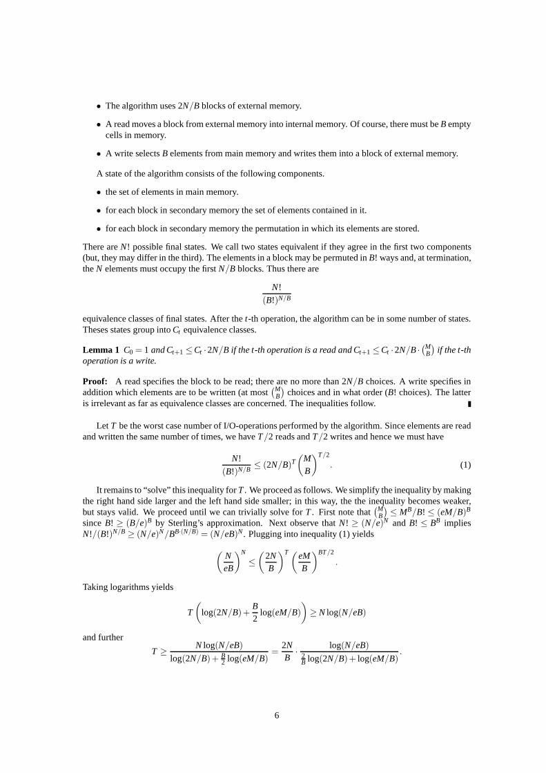
• The algorithm uses 2N/B blocks of external memory.

• A read moves a block from external memory into internal memory. Of course, there must beB emptycells in memory.

• A write selectsB elements from main memory and writes them into a block of external memory.

A state of the algorithm consists of the following components.

• the set of elements in main memory.

• for each block in secondary memory the set of elements contained in it.

• for each block in secondary memory the permutation in which its elements are stored.

There areN! possible final states. We call two states equivalent if theyagree in the first two components(but, they may differ in the third). The elements in a block may be permuted inB! ways and, at termination,theN elements must occupy the firstN/B blocks. Thus there are

N!

(B!)N/B

equivalence classes of final states. After thet-th operation, the algorithm can be in some number of states.Theses states group intoCt equivalence classes.

Lemma 1 C0 = 1 and Ct+1≤Ct ·2N/B if the t-th operation is a read and Ct+1≤Ct ·2N/B·(M

B

)

if the t-thoperation is a write.

Proof: A read specifies the block to be read; there are no more than 2N/B choices. A write specifies inaddition which elements are to be written (at most

(MB

)

choices and in what order (B! choices). The latteris irrelevant as far as equivalence classes are concerned. The inequalities follow.

Let T be the worst case number of I/O-operations performed by the algorithm. Since elements are readand written the same number of times, we haveT/2 reads andT/2 writes and hence we must have

N!

(B!)N/B≤ (2N/B)T

(

MB

)T/2

. (1)

It remains to “solve” this inequality forT. We proceed as follows. We simplify the inequality by makingthe right hand side larger and the left hand side smaller; in this way, the the inequality becomes weaker,but stays valid. We proceed until we can trivially solve forT. First note that

(MB

)

≤ MB/B! ≤ (eM/B)B

sinceB! ≥ (B/e)B by Sterling’s approximation. Next observe thatN! ≥ (N/e)N and B! ≤ BB impliesN!/(B!)N/B≥ (N/e)N/BB·(N/B) = (N/eB)N. Plugging into inequality (1) yields

(

NeB

)N

≤(

2NB

)T (eMB

)BT/2

.

Taking logarithms yields

T

(

log(2N/B)+B2

log(eM/B)

)

≥ N log(N/eB)

and further

T ≥ N log(N/eB)

log(2N/B)+ B2 log(eM/B)

=2NB· log(N/eB)

2B log(2N/B)+ log(eM/B)

.

6

Theorem 3 The number of I/Os required to permute N elements is at least

2NB· log(N/eB)

log(eM/B)+ 2B log(2N/B)

= Ω(

min

(

NB· log(N/B)

log(M/B),N

))

in the worst case.

Proof: We have already shown the first lower bound. For the second statement, we distinguish cases: iflog(eM/B)≥ 2

B log(2N/B), the first bound holds, if log(eM/B)≤ 2B log(2N/B), the second bound applies.

Sorting is no easier then permuting and hence the same lower bound applies. For practical values ofthe parameters, the second term in the denominator is negligible. For example, forB = 103, M = 108,N = 1012, logM/B = log105 ≈ 16 and(2/B) log(2N/B) ≤ 0.02. The lower bound agrees with the upperbound except for the second term in the denominator and the two occurrences of Euler’s constant.

The lower bound easily generalizes toD parallel disks. If we can permute withT I/Os with D disks,we can permute withTD I/Os with one disk. Thus the lower bound divides byD.

Theorem 4 The number of I/Os required to permute N elements with D parallel disks is at least

2NDB· log(N/eB)

log(eM/B)+ 2B log(2N/B)

in the worst case.

Note that this differs from the upper bound. The factor is(log(N/(DB)))/ log(M/(DB)) in the upperbound. AssumeB = 103, M = 108, N = 1012, andD = 102. Then the factor in the upper bound becomes(log107)/ log(103) = 7/3= 2.333 and the factor in the lower bound (ignoring the two occurrences ofe) is9/5 = 1.8.

From now on, we useSort(N) and Scan(N) as shorthands forO(N/B(log(N/B))/ log(M/B)) andO(N/B), respectively.

1.8.3 Sorting by Distribution

Exercise 4 Explore sorting by distribution. If the number N of elementsis less than M, use an optimalinternal sorting method. Otherwise, choose a random sampleof size approximately M/B, e.g., by choosingelements independently with probability M/(NB). Sort the sample internally and then distribute the inputinto buckets as defined by the sample. Allot a buffer of size B for each bucket. Sort each bucket recursively.

Assume first that the split into buckets is perfect, i.e., each bucket has size NB/M. What is the I/O-complexity of the method?

Then discuss deviations from perfection.

1.8.4 Optimal Sorting Methods

There are several sorting algorithms for parallel disks whose performance matches the lower bound; seeVitter’s book [Vit08].

1.9 PRAM-Simulation

This section is based on [CGG+95]. Chiang et al. showed how to simulate a PRAM in external memory.By way of the simulation, every PRAM algorithm gives rise to an external memory algorithm.

Before I describe the simulation, a general remark about simulation results. They are important for atleast two reasons.

• They structure the field and relate different computationalmodels to each other.

• They permit to transfer algorithms and lower bounds betweenmodels. If can simulate model A inmodel B, then algorithms for model A can be run on model B and lower bounds in model B translateinto lower bounds in model A.

7

1.9.1 List Ranking

The Internal Memory Algorithm: We assume that the list is singly-linked and that initially each elementknows its predecessor. We want to label each item with its distance to theheadof the list. We call the lastelement thetail of the list.

In internal memory, we traverse the list twice. In the first traversal, we determine the numbern of listitems. In the second scan, we assign distances.

Running this algorithm in external memory may lead toN IOs if N > M. If N > M, it may happen thatthe predecessor of the current list element (= the element just scanned) is never in main memory. Thus thetraversal of every link causes an IO.

We will show how to reduce the number of IOs toO(Sort(n)).Chiang et al. also claim the corresponding lower bound. It donot understand their argument.

A Recap of the Parallel Algorithm: Recall the parallel algorithm for list ranking. The input isa list ofn items;n is unknown. We want to label each item with its distance to theheadof the list. We call the lastelement thetail of the list.

Initially, each itemv knows its predecessorpred[v]. We associate an integerδ [v] with each list ele-ment and initialize it to one. During the course of the algorithm, we will change predecessor values byshortcutting. We maintain the invariant:

δ [v] is the distance fromv to pred[v] in the input list.

We update predecessor values by settingpred[v] to pred[pred[v]]. The invariant is maintained when we alsoexecuteδ [v] = δ [v]+ δ [pred[v]].

The algorithm works in two phases. In phase I, we shortcut thelist down to a list of two items, in phaseII, we assign the node labelsdist[v].

Phase I: Initially all list items are active.

while tail does not point to headdofor all active list itemsv do

choose a random bitbit[v]if bit[pred[v]] = 1 andbit[pred[pred[v]]] = 0 then

pred[v] becomes inactiveend ifif pred[v] becomes inactivethen

pred[v]← pred[pred[v]] andδ [v]← δ [v]+ δ [pred[v]].end ifobserve that thepred-value of elements that become inactive is not changed.

end forend whileOn average about 1/4-th of the list items become inactive. Notwo consecutive elements become inac-

tive and tail and head always stay active. Phase I ends when tail points to head.At the end of phase I, the pred-pointers define a tree:v points to the node it pointed to when it became

inactive. Since no two consecutive nodes become inactive ina round, the depth of this tree is no more thanthe number of rounds in phase I.

Phase II. Setdist[head] to zero.

for all list itemsv doif dist[pred[v]] is definedthen

dist[v]← dist[pred[v]]+ δ [v]end if

end for

Exercise 5 As formulated, the list items wait actively in phase II. i.e., they observe their predecessor andact as soon as the predecessor has a label. Change the algorithm such that waiting processors may beinactive, i.e., processors are woken up.

8

Hint: For each element v, maintain the list of items pointingto it. This list is sorted by time. In phaseII, wake up elements in inverse order of time.

Lemma 2 The algorithm above uses time O(logn) and work O(n). This requires a solution to the exercise.With active waiting the work is O(nlogn).

Proof: The number of active processors shrinks by a multiplicativefactor in each round of Phase I andgrows by the same factor in each round of Phase II.

A Mail System: I give a data centric view of the algorithm above. The data (= list items) sits in externalmemory (= a huge array) and each data item has an address (= theindex in this huge array). The data itemscommunicate with each other by exchanging messages, e.g., alist item may want to send information to itsneighbors or to get information from its neighbors.

Suppose every list item wants to send a message to its predecessor. It prepares an envelope, puts themessage into the envelope and writes the name (= index) of itspredecessor on the envelope. He hands theenvelope to the mail service, the mail services sort the mail, and distributes it.

The word sorting is meant literally. The envelopes are sorted by destination address and then distributedby a scan over all possible destinations.

Observe that we can allow that some list items send more than one message and that some list itemsreceive more than one message as long as the total number of messages isO(n).

Lemma 3 One round of message passing takes O(Sort(n)) IOs.

The External Memory Algorithm: The algorithm above uses only communication between adjacentlist items and hence can be implemented by message passing between adjacent list items. So every roundreduces to sorting and hence the algorithms runs inO(logNSort(N) I/Os. We will later show how to removethe logarithmic factor.

Phase I: Initially, all list items are active. We operate in(logN) rounds. Each rounds requires to send aconstant number of messages per list element.

Each active elementv chooses a random bit and sends the pair(v,bit(v) to is predecessor. Now, eachactive element knows its successor (in the list of active elements), its own bit and the bit of its successor.Thus it knows whether the successor will become inactive.

Each active element informs its successor, whether the successor becomes inactive or stays active.Each element that becomes inactive informs its successor about this fact and also sends the address of

and the distance to its predecessor to him. Nodes that becomeinactive also record the number of the roundin which they became inactive.

Active nodes that receive a message update their predecessor pointer and also the distance to theirpredecessor.

Phase I ends when tail points to head.Phase II: We label head with zero and tail with its distance tohead. Then we run time backwards, i.e.,

if phase I consisted ofK rounds, phase II consists of roundsK, K−1, down to 1.In roundi we first scan over all list items and wake up the ones that became inactive in roundi of phase

I. They send a message to their predecessor containing theirname. The predecessor sends back his label.

Lemma 4 The algorithm above requires O(logN ·Sort(N) IOs.

Compaction: We show how to shave off the logarithmic factor.We keep the active list in contiguous memory, i.e., if the active list containsa elements, these elements

reside ina/B disk blocks.If a≤ M, we use the internal method to rank the list. This is meaningful, but does not change the

asymptotics.We proceed as above and determine the elements that become inactive. Each inactive element points to

an active element and the active elements form a linear list.

9

We scan over the list and number the elements staying active starting at zero. We use two rounds ofmessage passing to inform each element staying active aboutthe number of its active predecessor.

We then create a new list consisting of copies of the list items staying active. Each copy stores a pointerto its original.

In this way, the length of the active list decreases exponentially. In each round, the length is reduced byapproximately the factor 3/4.

We come to phase II. Suppose, we have numbered the elements ofthe list created in round i+1 of phaseI. Each element informs his original about its number, the deactivated elements are activated, and distancesare propagated to them.

When the active list containsa elements, the number of IOs isO(Sort(a)). Thus the total number ofIOs is

∑i≥0

O(Sort(α iN)) = O(Sort(N))∑i≥0

α i = O(Sort(N)),

whereα = 3/4. We have thus shown:

Theorem 5 List ranking of a list of size N in external memory can be done with O(Sort(N)) IOs.

Remark: Of course, we should stop the recursion, once the active elements fit into main memory. Thisdoes not change the asymptotics though.

1.9.2 A General Simulation

We consider a PRAM withN processors and a global memory of sizeO(N). We useM[i] to denote thememory cell with indexi. TheN processors work in parallel. In each step, each processor first reads fromor writes to memory and performs some local computation on its registers, and finally writes to memory.There are a finite number of registers per processor. We assume that each processor has an address registerand useRi to denote the address register of processori. Processori then load/stores memory cellM[Ri ].

The external memory algorithm uses a single CPU; it stores the arrayM in external memory. It alsohas an arrayP of blocks of constant size;P[i] contains the registers of thei-th PRAM processor. A singlestep of the PRAM is simulated as follows.

1. We scan overP and generate tuples(Ri ,READ/WRITE, i,vi), where the second component indicateswhether processori wants to read or write. In the case of WRITE, the fourth component is the valueto be written.

2. We sort the pairs lexicographically, where READ precedesWRITE. Call the resulting sorted listS.Scontains the memory accesses sorted by address, READs to thesame address precede the writes.

3. We scan overSandM in parallel. When we scan over a tuple(Ri ,R/W, i,vi) in S, the scan overM isat positionRi in M. If the tuple stands for a read, we generate the pair(i,M[Ri ]). If the pair standsfor a write, we writevi into M[Ri ].

4. We sort the pairs(i,M[Ri ]) by first element. Call the sorted listT.

5. We scan overT andP in lock-step fashion. For each indexi, we are performing the local computationof PRAM processori usingP[i] and the pair(i,M[Ri ]).

The simulation of each PRAM-step takesSort(N) I/Os. We obtain:

Theorem 6 A PRAM-algorithm using N processors, a memory of size N, and time T can be simulated withO(T ·Sort(N)) I/Os.

Exercise 6 Generalize the theorem to PRAM algorithms that use a memory of size M≫ N.

Some PRAM-algorithms use an exponentially decreasing number of processors. For them, the simula-tion can be improved.

10

Theorem 7 Consider a PRAM-algorithm using a memory of size N and operating in logaN phases forsome constant a> 1. The i-th phase,0≤ i ≤ logaN, takes time Ti and uses N/ai processors. Let T= ∑i Ti .The external memory simulation requires

∑i

(

Ti/aiSort(N)+TiScan(N))

I/Os. If Ti = T0 for all i and some T0, the bound becomes

T0Sort(N)+TScan(N).

Proof: In the i-th phase, onlyN/ai elements need to be sorted. Thus thei-th phase takesTi(Sort(N/ai)+Scan(N) I/Os. Since,Sort(N/ai)≤ 1/aiSort(N), the first bound follows. IfTi = T0 for all i, we have

∑0≤i≤logaN

T0Sort(N/ai)≤ T0 ∑0≤i≤loga N

1ai Sort(N) = T0Sort(N).

1.9.3 Applications

Exercise 7 Develop an external memory algorithm for connected components. Start from the PRAM-algorithm presented in class.

1.10 BFS and DFS

For sequential computation, DFS and BFS are basic ingredients of many graph algorithms. No efficientrealization of DFS is known. For BFS, the situation is somewhat better, but still unsatisfactory.

1.10.1 Naive BFS

The sequential version of BFS is easy to state. The algorithmoperates in phases and maintains a queueQand an arrayunreached. In the i-th phasei ≥ 0 all nodes at distancei from the source node are scanned.For each such node the edges out of it are scanned. The targetsof the edges leading to unreached nodesform the next layer.

Q′← sunreached[v]← true for all v; unreached[s]← falsewhile Q′ 6= /0 do

Q←Q′ andQ′← /0while Q 6= /0 do

v← first element ofQ; deletev from Qfor all neighborsw of v do

if unreached[w] thenaddw to the end ofQ′; unreached[w]← false;

end ifend for

end whileend whileWe assume the standard storage layout for an undirected graph. The edges are stored in an arrayE of

size 2m. For each nodev, the edges incident onv are stored in a segment of lengthdv starting atfv. Thevaluesfv are stored in an arrayF of sizen.

In the above code, random access is used twice: When we removea nodev from Q, we need to accessF [v] and thenE[F[v]]. We then scan thedv edges incident tov. For each edge(v,w) we need to accessunreached[w]. In the worst case each random access results in a disk accessand hence naive BFS takesΩ(n+m) I/Os in the worst case. Naive BFS is useless for graphs that donot fit into memory.

11

1.10.2 Munagala and Ranade

Munagala and Ranade [MR99] observed that the test whetherw is unreached can be postponed to the endof a phase. They maintain two additional setsLp andLc; Lc contains the current layer,Lp contains thepreceding layer.Lp andLc are sorted by node number. There is no arrayunreached.

Lemma 5 Let Li be the nodes at distance i from a source s in an undirected graph G. Then

Li+1 = w; there is v∈ Li with vw∈ E \ (Li ∪Li−1).

Proof: If w is in Li+1 then there must be an edge from a nodev∈ Li to w andw cannot belong to any layerL j , j ≤ i. We conclude thatLi+1 is contained in the set on the right-hand side of the equation.

Since the edges out of nodes inLi can only go to nodes inLi−1∪Li ∪Li+1, equality holds.

Lp andLc are initialized to the empty set ands, respectively. When the edges out ofv are scanned,all targetsw are added toQ′.

At the end of a phaseQ′ is a multi-set of nodes. We obtain the next layer by removing duplicates fromQ′ and by removing all nodes inLp∪Lc from Q′. We sortQ′, and then scan the sorted version ofQ′ andLp

andLc in parallel.Letd(Li) = ∑v∈Li

dv be the total degree of the nodes inLi . Then the number of I/Os required to constructthe next layer is

Sort(d(Li))+Scan(Li−1)+Scan(Li).

Since every node belongs to exactly one layer and each edge isincident to at most two layers, the summa-tion over all layers results inO(Sort(m))+Scan(n)) I/Os.

It remains to analyze the I/Os required to access first elements of adjacency lists. We bound the numberin two ways. First, there is at most one I/O per adjacency listfor a total ofn I/Os. Second, when a phasestarts, the nodes in the current layer are available in sorted order. Thus, finding their first edges can take nomore than a scan of all edges. This bounds the number of I/Os byO(Scan(m) ·diam(G)), wherediam(G)is the diameter2 of G.

Theorem 8 The number of I/Os required by the Munagala-Ranade version of breadth-first is no more thanO(min(n,Scan(m)diam(G))+Sort(m)).

1.10.3 Mehlhorn and Meyer

Meyer and Mehlhorn [MM02] reduced the number of I/Os further. The idea is simple. They first decom-pose the graph into subgraphs of small diameter, sayk, wherek is a carefully chosen parameter. Then theyreorder the adjacency lists such that the nodes and edges of each subgraph are stored compactly. Finally,they run BFS on the rearranged graph and exploit the fact thatonce some node of a subgraph is reached bythe search, the entire subgraph will be explored in the nextk phases. We next give the details.

The Decomposition into Small Diameter Subgraphs We select a subsetS of seed nodes by puttingeach node intoSwith probabilityp; p will be determined later. For technical reasons, we also puts into S.Then the expected size ofS is 1+np. For each nodeu in S, we construct a subgraphFu.

We run BFS starting at the nodes inS, i.e., we initialize the queue withSand then run Munagala-RanadeBFS. For each nodev, we record the seed node from which it is reached. Also, whenv is reached fromu∈S, we move the edges out ofv to the subgraph3 Fu. In this way, the representation ofG becomes smalleras the algorithm progresses. The adjacency list of a nodev is scannedℓv times, whereℓv is the index of thelayer to whichv is added.

Lemma 6 The expected value ofℓv is no more than1/p.

2The diameter of a graph is the longest shortest path between any two vertices.3In order to do this efficiently, we keep a buffer of one block for eachu∈ S.

12

Proof: Let v = u1,u2, . . . ,ur = s be a shortest path fromv to s and leti be the smallest index such thatui

belongs toS. Since nodes are put intoS independently and with probabilityp, the expected value ofi is atmost 1/p. (the value would be exactly 1/p if r would be infinite).

Lemma 7 The expected number of I/Os performed for decomposing the graph into small diameter sub-graphs is O(Scan(m)/p+Sort(m)).

We store the subgraphsFu, u∈ S, one after the other in external memory. We enhance the representa-tions somewhat. We store each edge(v,w) as a three-tuple(v,w, fw), where fw is the location where therepresentation of the subgraphFu containingw starts.

BFS We next describe how to implement BFS. We run Munagala-Ranade with one change. We maintaina setH containing the representations of all subgraphsFu intersecting the current layer;H is ordered bynode number.

We construct the next layer as follows. We scan over the nodesin the current layerLc andH in parallel.We obtain the multi-set of targets of edges out of the currentlayer. Edges scanned are removed fromH.We sort the multi-set and remove duplicates. We scan over theresulting set andLp andLc and obtain thesorted setLp of nodes of the next layer. We scanLp andH in parallel and find the vertices inLp that are notyet in H. For them, we fetch theFu containing it (this requires one random access perFu) and store themin a temporary fileF ′. We sortF ′ by node number and merge it intoH.

Lemma 8 The expected number of I/Os required by the Mehlhorn-Meyer version of BFS is O(np+Scan(m)/p+Sort(m)).

Proof: When some nodev′ in Fu is reached,Fu is added toH. This requires(1+ Scan(|Fu|)) I/Os foraddingFu to F ′. ThenSort(|F ′|) I/Os are needed to sortF ′. Finally, we need to scanF ′ andH to mergeF ′

into H. The expected number ofFu’s is 1+np and eachFu is added once. Thus the sorting and scanningtimes for theFu’s add up toO(1+np+Sort(m)).

The adjacency list of a nodev in Fu stays for no more thand(v′,u)+ d(u,v) phases inH. Thus onaverage, an adjacency list is scannedO(1/p) times. This adds up toO(Scan(m)/p) I/Os.

Preprocessing takesO(Scan(m)/p+Sort(m)) I/Os.

We choosep such thatnp= Scan(m)/p, i.e., p = min(1,√

Scan(m)/n) and obtain:

Theorem 9 BFS can be performed with O(Sort(m)+√

nm/B) I/Os.

Proof: If Scan(m)≥ n, we setp = 1. Also,n≤Scan(m)≤Sort(m) and the bound follows. IfScan(m)≤n, we setp =

√

Scan(m)/n. Thennp= Scan(m)/p=√

nScan(m) =√

nm/B.

Let us work through a concrete example. Letn = 1012, m = 1013 andB = 103 andM = 109. ThenSort(m) = 1010(log(1010))/ log(106)≤ 2 ·1010 and

√

nm/B=√

1020 = 1010.In comparison, Munagala-Ranade may require 1012 I/Os.

Exercise 8 A deterministic method for decomposing a graph: Construct the Euler tour of a spanning tree.Decompose the Euler tour into segments of length k. Nodes appearing in more than one segment areassigned to one of the segments arbitrarily.

1.10.4 Experimental Comparison

See [ADM06, AMO07]. For small diameter graphs, Munagala-Ranade is better. For large diameter graphs,Mehlhorn-Meyer is better.

1.10.5 Lower Bounds

Munagala and Ranade [MR99] prove a lower bound ofΩ((m/n)Sort(n)).

13

1.10.6 DFS

Completely open.

1.11 Other Graph Problems

Connected components, spanning trees, biconnected components can be done withSort(m) I/Os. See thearticle by Katriel and Meyer in [MSS03].

2 Searching: B-trees, Buffer Trees and van-Emde Boas Trees

2.1 B-Trees

B-trees were invented by Bayer and McCreight [BM72] in 72. They are used in many data bases. In yourdata structure course you learned about (2,4)-trees. B-trees are a variant of them.

All root-to-leaf path have the same length. The degree of every node is at mostb, the degree of eachnode (except for the root) is at leasta, the degree of the root is at least 2. The parameterb is chosen suchthat a node fits into a memory block, i.e.,b= Θ(B); a= b/2, so that the machinery of balanced trees works.The depth of a tree withN leaves isΘ(logaN) = Θ(logBN).

Lemma 9 B-trees support searches, inserts and deletes withΘ(logBN) I/Os per operation.

2.2 Cache-Oblivious Search Trees

The disadvantage ofB-trees is that they require knowledge ofB.van-Emde-Boas [PEB77] invented a tree layout (for a completely different purpose) that gives good

performance for every value ofB; B is only used in the analysis, but not in the program. This is what iscalled acache-obliviousalgorithm.

The idea is simple. Consider a complete binary tree of heighth, where 2k < h≤ 2k+1. We split it intoa top tree of heighth− 2k and 2h−2k

bottom trees of height 2k each. Each leaf node in the top tree haspointers to its two children bottom trees. The memory layoutis as follows.

We first store the top tree and then the bottom trees.For the top tree and the bottom trees, we use the same idea recursively.For a tree of size 15 this results in the following numbering of the vertices.

12 3

4 7 10 135 6 8 9 11 12 14 15

The basic building blocks of van-Emde-Boas trees are complete binary trees of height 1, 2, 4, 8, 16,and so on.

If the height of a tree is a power of two, the bottom and top trees have half the height. If the height isnot a power of two, we make the height of the bottom trees a power of two (= the first one in the binaryrepresentation of the height) and give the top tree the remaining height (= the other bits in the binaryrepresentation of the height)

Lemma 10 Searching in a complete binary tree of size N in van-Emde-Boas layout takes O(logBN) I/Os.

Proof: Let ℓ be such that trees of heightL = 2ℓ fit into a memory block, but trees of height 22ℓ do not.Then 2L ≤ B < 22L and henceL≤ logB < 2L. ThusL = Θ(logB).

Conceptually, decompose the search tree of heighth = logN into trees of heightL. A search traverses(logN)/L = O(logBN) trees. Since trees of heightL fit into a memory block and hence span at most twomemory blocks by virtue of the layout, the result follows.

14

There is also a dynamic version of cache-aware search trees with the same performance.

Warning: The colloquial way of talking about van-Emde-Boas like strategies is to say that a problemof sizen is split into

√n problems of size

√n. Of course, this is only possible isn is a square. Moreover,

in order to continue the recursive strategy,√

n also needs to be square, and so on. The colloquial way onlyapplies to input sizesn that are of the formn = 22k

for some integerk.In our description above, we split a tree of heighth into bottom trees of height 2ℓ, where 2ℓ < h≤ 2(ℓ+1)

and a top tree of heighth−2ℓ. The colloquial approach now applies to the bottom trees.We will follow the colloquial approach in our discussion of funnel sort. But be aware, that strictly

speaking we are not giving proofs but plausibility arguments.In the analysis of many bisection algorithms, one starts with the sentence: Let us assume w.l.o.g. that

n is a power of two. This is ok, since the smallest power of two isat most twice as large asn and sincebisection stays within powers of two. The same argument doesnot appy to van-Emde-Boas like strategies.The smallest number of the from 22k

greater or equal ton may be as large asn2. The smallest square greateror equal ton is no larger than

⌈√n⌉2≤ (

√n+1)2 = n+2

√n+1 = n

(

1+2√

n+1n

)

.

Replacing at each level of the recursionn by the smallest square greater or equal ton is a feasible strategy.To be on the safe side, one should check whether the solution of the recursion still applies, i.e., whether thesolution to

T(n) = f (n)+√

nT(√

n)

is also a solution (at least in order of magnitude) to

T(n) = f (n)+⌈√

n⌉

T(⌈√

n⌉

).

We leave it to the reader to check this in what follows.

3 Cache-Oblivious Algorithms

The cache-oblivious model was introduced in [FLPR99]. Cache-oblivious algorithms cannot useM andBin the program code. Nevertheless, they work well under the tall cache assumption.

Frigo et al. gave cache-oblivious algorithms for matrix multiplication, sorting, and Fourier transform.Since their paper, many more cache-oblivious algorithms were developed, in particular for search trees,priority queues, and simple geometry problems. We refer ourstudents to the survey paper by Lars Arge,Gerth Brodal, and Rolf Fagerberg.

3.1 Tall Cache Assumption

Main memory consists ofM/B blocks of sizeB. In the case of caches,M/B is called the height of thecache andB is called the width of the cache. The tall cache assumption states that the height is larger thanthe width, i.e.,M/B≥ B. In other words,M ≥ B2. Many results about cache-oblivious algorithms holdtrue under the weaker assumption thatM ≥ B1+γ for some constantγ > 0.

In the analysis of funnel sort, I will use the assumption M≥ B5/2.Brodal and Fagerberg showed that the tall cache assumption is necessary for many results in the area.

3.2 Cache Replacement Strategy

When a cache line (this is what we called block in external memory algorithms) is brought into a full cache,one of the cache line present in the cache must be evicted fromthe cache. In external memory algorithms,the programmer controls which block is overwritten (evicted). We no longer have this control.

We first assume an optimal cache replacement policy, i.e., the line, for which the next access is furthestin the future, is evicted. Of course, optimal replacement isimpossible to implement.

15

The standard replacement strategy is least recently used (LRU). It evicts the cache line whose last usageis furthest in the past.

Sleator and Tarjan [ST85] showed that LRU-caches with twiceas many cache lines simulate an optimalcache efficiently. More precisely,

Theorem 10 Let mLRU and mOPT be the number of cache lines available to LRU and OPT, respectively.Then the number of cache faults incurred by LRU in processinga sequence s of requests is at

mLRU

mLRU−mOPT+1FOPT+mOPT,

where FOPT is the number of cache fault incurred by the optimal algorithm.

Proof: After the first access, the memories of LRU and OPT have at least one cache line in common,namely the cache line just accessed.

Consider a subsequencet of s of requests in which LRU incursf cache faults, wheref ≤ mLRU andlet x be the cache line accessed just beforet. Then, at the beginning oft, x is in the memory of LRU andthe memory of OPT. If LRU faults twice on the same page int, at leastmLRU + 1 distinct cache lines areaccessed int. This is also true if LRU faults onx duringt. If neither is the case, LRU faults on at leastfdistinct pages int, none of which isx. In either case, OPT must fault at leastf −mOPT+1 times int.

We partitions into subsequencess1, s2, . . . , sk as follows: In the first subsequences1, LRU incurs atmostmLRU pages faults and in all other subsequences, LRU incurs exactly mLRU page faults. Letf be thenumber of page faults of LRU ins1. Then OPT faults at leastf −mOPT+1 times ins0. The bound follows.

3.3 Funnel Sort

Funnel sort is a variant of merge sort.

1. We split the input of sizeN into N1/3 contiguous parts of sizeN2/3.

2. We sort each part recursively.

3. We merge the resultingN1/3 sorted sequences into a single sorted sequence usingfunnel merge.

We have the following recurrence for the number of I/Os required by funnel sort.

T(N) =

N1/3T(N2/3)+Cost of funnel merge ifN > dM

O(N/B) if N≤ dM,

where the constantd is such that funnel sort fordM elements fits into cache.

Exercise 9 Explore alternative ways of splitting the input. Split intoNα sequences of length N1−α . Whichα work?

As in external merge sort, we want to use a tournament for merging the sequences. However, we knowneither the size of the cache nor the width of the cache. Therefore we use the van-Emde-Boas layout forthe tournament.

Assume that subtournaments of sizeJ fit into main memory. We view the overall tournament as beingcomprised of tournaments of sizeJ. We separate the subtournaments by buffers and operate the subtourna-ments in cyclic fashion. First we operate the subtournaments in the bottom layer. This will fill the buffersbetween the bottom layer and the next to bottom layer. Then weoperate the next to bottom layer; this willfill the buffers between the second and the third layer and partially empty the buffers between the first andthe second layer. We work our way up to the topmost layer and produce output. We repeat as long as thereare elements in the system.

How large should we choose the buffers? In order to operate a subtournament, we need to bring it intomain memory. We want to amortize the cost of bringing the subtournament into memory over the elementsprocessed by the subtournament. Thus, if bringing a subtournament into memory has costC, we shouldprocess at leastCB elements with it (because bringingCB elements into memory has costC).

How do we cope with the fact that we do not knowJ? We build our structure recursively.

16

3.3.1 Funnel Merge

We describe Funnel Merge withK inputs. The base case isK = 2. Then funnel merge is the standardalgorithm for merging two sequences.

For largerK, we build funnel mergeF(K) from (1+√

K) funnel mergers for√

K inputs each. We feed√K input sequences into each one of the bottom level mergers. The output of each bottom level merger is

fed into a buffer which in turn feeds into the top level merger. We have√

K buffers of sizeK2 each. Thusthe total area for the buffers isK5/2.

The memory layout is as in van-Emde-Boas trees. We allocate the top merger, the buffers, and thebottom trees in contiguous memory. The spaceS(K) required forF(K) satisfies the recurrence

S(K) = (1+√

K)S(√

K)+K5/2 = K5/2 +(1+K1/2)(K5/2·1/2 +(1+K1/4)S(K1/4)+ . . .≤ cK5/2

for a small constantc. We allocate spacecK5/2 for F(K).We operateF(K) as follows. We haveK input sequences. It is assumed that their total length is at least

K4. Observe that this is true for the merger in funnel sort. There, we use aF(N1/3) merger and feed itsequences of total lengthN.

The F(K)-operation: We perform the following cycleK times.

• Operate each of the bottom mergersF(√

K) in turn until its output buffer is full.

• Operate the top mergerF(√

K) for K2 steps or until the output buffer of the containingF(K)-mergeris full. Observe that the buffers connecting the bottom mergers and the top merger have sizeK2 andhence we can operate the top merger forK2 steps.

The outermost merger is aF(N1/3)-merger. We invoke it once. Since its output buffer will never getfull, we extractN2/3 elements per round and henceN elements in total. Inner mergers are used unevenly.The number of elements extracted depends on the number of empty locations in the output buffer. Thisnumber may be as small as zero. However, amortized over all invocations of anF(K)-merger,K3 ele-ments are processed per invocation. This will allow us to amortize the initialization cost over the elementsprocessed.

Lemma 11 For all K: if a F (K)-merger is invokedℓ times then a total ofℓK2 elements flow through eachinput. The total number of elements flowing through the merger is ℓK3.

Proof: We use induction onK downwards. TheN1/3-merger is invokedℓ = 1 times andN2/3 elementsflow through each input.

Assume now that the claim is true forF(K)-mergers. TheF(√

K)-mergers comprising aF(K)-mergerare invokedℓ′ = ℓK times. By induction hypothesis, at leastℓK2 elements flow through each input of theF(K)-merger and hence through each input of theF(

√K) merger. Since

ℓK2 = ℓKK = ℓ′(K1/2)2,

the induction step is completed.A F(K)-merger hasK inputs. Thus a total ofℓK3 elements flow through anF(K)-merger.

We come to the analysis. LetJ be largest (according to our recursive strategy) such thatF(J) usesspace at mostM/4. Then

cJ5/2≤ M4

< cJ5.

There areJ input buffers ofF(J) and the memory is large enough to holdF(J) plus one cache line perinput buffer. This follows from

JB≤ 2/5

√

M4c

√M ≤ M√

4c≤ M

2;

here the first inequality uses the tall cache assumptionB≤√

M.

17

What is the cost ofone F(J)-operation? We split the cost in the initialization cost andthe cost ofmoving elements through the merger.

Bringing F(J) plus one cache line per input buffer (we need to count one I/O per input buffer sinceinput buffers are not guaranteed to feed any elements to their subsequent merger and hence we cannotdirectly amortize the initialization over the elements processed) into the cache requiresO(J2/B+J) I/Os.SinceJ5 = Ω(M) = Ω(B5/2) (here we use our tall cache assumptionM ≥ B5/2 and henceJ2 = Ω(B), wecan boundO(J2/B+J) by O(J3/B).

OnceF(J) plus one line per input buffer is in the cache, we only pay for moving elements into the inputbuffer and out of the output buffer. If aF(J)-merger is invokedℓ times a totalℓJ3 elements flow throughthe merger. The cost of bringing these elements into cache and writing them back isO(ℓJ3/B). The cost ofsetting up theF(J)-mergerℓ times is no larger. Thus the cost of operating theF(J)-merger isO(1/B) I/Osper element processed.

View a funnelF(K) as being comprised ofF(J) funnels. The height ofF(K) viewed as a binary tree islogK, the height ofF(J) is logJ, and hence any element is processed by(logK)/(logJ) = logJ K funnelsF(J). Thus anF(K)-operation processesK3 elements with a total number of

O

(

K3

BlogM K

)

= O

(

K3

BlogM/B

K3

B

)

I/Os. Here we used that logJ = Θ(logM), that logM = Θ(log(M/B)) by the tall cache assumption and thatlogK = O(log(K3/B)) sinceK2≥ J2≥ B.

3.3.2 Analysis of Funnel Sort

We have the following recurrence for the number of I/Os required by funnel sort.

T(N) =

N1/3T(N2/3)+ NB logM/B

NB if N > dM

O(N/B) if N≤ dM,

where the constantd is such that funnel sort fordM elements fits into cache.The total leaf cost of this recursion isO(N/B).With respect to the inner nodes, the cost at the root dominates, as expansion of the recursion shows.

T(N) = N1/3T(N2/3)+NB

logM/BNB

= N1/3

(

N2/9T(N4/9)+N2/3

BlogM/B

N2/3

B

)

+NB

logM/BNB

≤ N5/9T(N4/9)+NB

(

1+23

)

logM/BNB

≤ NB

(

1+23

+49

+827

+ ...

)

logM/BNB

Lemma 12 Funnel sort with optimal cache replacement strategy sorts with

O

(

NB

logM/BNB

)

cache faults.

Theorem 11 Funnel sort with LRU cache replacement sorts with

O

(

NB

logM/BNB

)

cache faults.

Proof: ReplacingM by M/2 does not change the asymptotics.

18

3.4 Funnel Priority Queues

4 Matrix Multiplication

4.1 External Memory

The standard layout for matrices is row-major order, i.e., amatrixA of sizen by n is stored as the sequenceA1,1, . . .A1,n,A2,1, . . . ,A2,n, . . . .

Exercise 10 How many I/Os are required for matrix multiplication, when matrices are stored in row-majororder?

How many I/Os are required for a matrix product AB, when A is stored in row-major order and B isstored in column-major order?

Exercise 11 Show that one can transpose a N by N matrix with Sort(N2) IOs. Show that one can transformrow-major layout into column-major layout with Sort(N2) IOs.

Exercise 12 (Block Layout of Matrices) Divide A into square submatricesof size√

M×√

M. Store theelements in each submatrix contiguously

Visualize the layout for a 8 by 8 matrix that is split into submatrices of size 2 by 2, i.e., draw a 8 by 8grid and number the grid cells in the order in which they appear in the layout.

What is the IO-complexity of matrix multiplication when matrices are stored in block layout?How does this compare to the bound obtained in the first exercise?

Exercise 13 (Recursive Layout of Matrices) Split a matrix A into four matrices A1,1, A1,2, A2,1, A2,2. StoreA as A1,1 followed by A1,2 followed by . . . . Use the same technique recursively on the submatrices.

Visualize the layout for a 8 by 8 matrix.What is the IO-complexity of matrix multiplication when matrices are stored in block layout?Does the algorithm need to know M?How does this compare to the bounds obtained in the two preceding exercises?

Exercise 14 Redo the preceding exercise for Strassen matrix multiplication.

A Lower Bound We prove a lower bound ofΩ( nM1/2B

IOs under the following assumption. Each arrayelement is associated to a storage location. For each triple(i, j,k), 1≤ i, j,k≤ n, it is necessary thatAi, j

andB j ,k andCi,k aresimultaneouslyin main memory.Observe that the model is quite restrictive, e.g., Strassenmatrix multiplication is not covered by the

model.We start with a combinatorial lemma.

Lemma 13 An undirected graph with m edges contains at most4m3/2 triangles, i.e., triples(u,v,w) ofdistinct vertices such that uv, vw and uw are edges of G

Proof: For each triangleT, we will distribute a charge of 1 over the edges ofG. Then we will upperbound the total charge.

We identify the vertices with the integers 1 ton. For each triangleu(T) be the smallest vertex of thetriangle.

Consider a fixed vertexu and consider the trianglesT with u = u(T). If the degree ofu is at most√

m,we charge 1/2 to each edge ofT incident tou. If the degree ofu is more that

√m, we charge 1/

√m to each

edge incident tou.Consider now an edgee= vw. How much is charged to it? We estimate the charge due to endpoint v.

If the degree ofv is at most√

m thene picks up no charge of the second kind and at most√

m/2 chargeof the first kind, because there are at most

√m choices for the other edge in the triangle incident tov. If

the degree ofv is more than√

m thene picks up no charge of the first kind and at mostm/√

m charge ofthe second kind because there are at mostm choices for the triangle edge not incident tov. Thus the totalcharge toebecause of endpointv is at most 2

√m.

19

The total charge to all edges is at most 4m3/2.

Theorem 12 In the model defined above, the IO-complexity of matrix multiplication is at leastΩ(n3/(M1/2B).

Proof: We partition execution into slices ofM/B IOs. In a slice, we can read/write at mostM arrayelements. Thus at most 2M array elements “meet” during a slice, namely, theM elements that were inmemory at the beginning of the slide plus the up toM elements that were read in the slice. The 2M arrayelements can form at most 4· (2M)3/2 triangles. Since we need to formn3 triangles, there must be at least

Ω(

n3

M3/2

)

slices.

Multi-Core Algorithms for Matrix Operations: Search the literature.

5 Interlude: Pivot Selection for Distribution Sort

Distribution sort operates recursively. It selects a set ofd pivots and sorts them. Thed pivots defined+1buckets, one for each interval between adjacent pivots and the buckets for the elements smaller than the firstpivot and larger than the last pivot, respectively. The input is distributed into these buckets. The bucketsare then sorted recursively.

For parallel and external memory algorithms it is importantto control the maximum bucket size asit determines the recursion depth and load balancing between processors. So one needs a nearly equallyspaced set of pivots.

5.1 Quicksort

Here we need a single pivot.

Randomized Selection: If the pivot element is chosen at random, the expected size ofthe larger sub-problem is 3n/4, wheren is the problem size.

We obtain a much better control over the larger subproblem byselecting 2k+1 random elements andtaking their median as the pivot.

For example, what is the probability that the smaller subproblem has sizen/8 or smaller? This can onlyhappen if at leastk+1 of the chosen elements belong to then/8 smallest or largest elements of the input.Thus this probability is

≤ 2 ·(n/8

k+1

)

·(n−(k+1)

k

)

( n2k+1

) ;

observe that we must choosek+ 1 elements among the extremen/8, the remainingk elements out of theremainingn− (k+1) elements. A short calculation yields shows4

2 ·(n/8

k+1

)

·(n−(k+1)

k

)

( n2k+1

) = 2 · [n/8]k+1[n− (k+1)]k(2k+1)!(k+1)!k![n]2k+1

= 2 · [n/8]k+1

[n]k+1·(

2k+1k

)

≤ 2 ·(

n/8n

)k+1

·22k+1

= 2−(k+1)

4[n]k = n(n−1) · (n−k+1).

20

since(y

x

)

≤ (1+1)y = 2y for integersx andy. A shorter but incorrect argument ignores that we are samplingwithout replacement. We must choose at leastk+1 elements among either the smallestn/8 or the largestn/8 and hence the probability is at most

2(1/8)k+1 ·(

2k+1k

)

≤ 2 ·2−3k−322k+1≤ 2−k−1.

Actually, the above is quite crude. I will next estimate thatthe median of 2k+1 chosen elements is thei-th largest element of the input file. We will see that this probability is small if i 6∈ (1/2− ε,1/2+ ε)nandk is at least logarithmic inn.

Lemma 14 Let pi be the probability that the median of a random sample of2k+1 elements is equal to thei-th largest element. Forε > 0, a positive constant, k≥ (C/2ε2) lnn, k/n≤ ε2, k < n/3−1, i = xn, andx 6∈ (1/2− ε,1/2+ ε), we have

pi ≤2nC .

Under the same assumption, the probability that the median of the sample does not have rank in(1/2−ε,1/2+ ε)n is bounded by2/nC−1.

Proof: We may assumei ≤ n/2 by symmetry. If the median of the 2k+1 chosen elements is equal to thei-th largest element, we have drawnk samples from the firsti−1 elements andk samples from the largestn− i elements and we have chosen thei-th element. Thus

pi =

(i−1k

)(n−ik

)

( n2k+1

)

since there are( n

2k+1

)

ways of choosing the 2k+ 1 elements amongn elements, and there are(i−1

k

)

and(n−i

k

)

ways of choosingk elements out ofi−1 andn− i, respectively. Ifk≥ i, pi is clearly zero. So assumei < k. Expanding the binomial coefficients yields

pi =[i−1]k[n− i]k(2k+1)!

k!k![n]2k

=[i−1]k[n− i]k(k+1)

[n]k[n−k]k(n−2k)

(

2k+1k

)

≤ 2 ·4k(

i(n− i)n(n−k)

)k

since(2k+1

k

)

≤ (1+1)2k+1 = 2·4k and(a−d)/(b−d)≤ a/b for d≤ a≤ b. Let i = nxwith x≤ 1/2. Then

pi ≤ 2 ·(

4x(1−x)1−k/n

)k

≤ 2 ·(

1−4ε2

1−k/n

)k

≤ 2 ·ek(ln(1−4ε2)−ln(1−k/n)) ≤ 2 ·ek(−4ε2+2k/n) ≤ 2 ·e−2ε2k = 2 ·e−C lnn =2nC

since−2x≤ ln(1−x)≤−x for 0≤ x≤ 1/4.The second claim follows since there are less thann choices fori.

Deterministic Selection: The following technique was first used in the linear-time median algorithm.Divide the input into groups of five elements. Letmi be the median of thei-the group and letm∗ be the

median of the medians.Assume for simplicity, that we have an odd number of groups, say we have 2k+ 1 groups andn =

5(2k+ 1) elements. Thenk of the mi ’s are smaller thanm∗. For eachmi smaller thanm∗, at least threeelements in the group are smaller thanm∗. Thus the number of elements smaller thanm∗ is at least

3k+2≥ 3k+210k+5

n≥ 0.3 ·n.

By symmetry, at least 0.3 ·n elements are larger thanm∗.

21

5.2 Multi-Way Partitioning

In parallel and external memory sorting we need multi-way partitioning in order to keep the recusion depthlow and to balance the load among processors. We generalize the solutions given above for the median.

We want to choose a sample of sized such that each bucket defined by the sample contains aboutn/(d+1) elements of the input set.

A Randomized Solution: We choose a random subsetT of size(k−1)(d+1)+d from the input set andtake the elements of rankik, 1≤ i ≤ d, in this set.

Lemma 15 Let C> 1 be a constant. If x≥ 1 is such that4ex/ex/2≤ 1/e, L= xn/(d+1), k(d+1)+L≤n/2, k≥ (C+2) lnn, then the probability that some bucket contains more than Lelements is at most1/nC.

Proof: Let I be the input set in sorted order. If a bucket containsL or more elements then there mustbe contiguous subset ofI of lengthL from which at mostk−1 elements are chosen. There aren−L + 1choices for the first element inL. Thus the probability that some bucket hasL or more elements is boundedby

p :=n ∑i≤k−1

pi where pi :=

(Li

)( n−Lk(d+1)−1−i

)

( nk(d+1)−1

) .

We estimatepi .

pi =[L]i(n−L)!(k(d+1)−1)!(n−k(d+1)+1)!

i!(k(d+1)−1− i)!(n−L−k(d+1)+1+ i)!n!

≤(

eLi

)i (n−L)!(k(d+1)−1)!(n−k(d+1)+1)!(k(d+1)−1− i)!(n−L−k(d+1)+1+ i)!n!

sincei! ≥ (i/e)i

≤(

eLi

)i (k(d+1)−1)i[n−k(d+1)+1]L−i

[n]L

≤(

eLk(d+1)

i

)i [n−k(d+1)+1]L[n]L[n−k(d+1)+1− (L− i)]i

≤(

eLk(d+1)

i(n−k(d+1)−L)

)i(n−k(d+1)+1n

)L

sincea−xb−x

≤ ab

for x≤ a < b.

Next observe that(

n−k(d+1)+1n

)L

= e−L ln(1−(k(d+1)−1)/n) = e−Lk(d+1)/(2n) = e−xk/2,

sincek(d+1)−1≥ k(d+1)/2 and ln(1−x)≤−x for x≥ 0, and that

(

eLk(d+1)

i(n−k(d+1)−L)

)i

≤(

exnki(n/2))

)i

≤ (4ex)k

since(k/i)i ≤ ek. Let y = k/i. Theny≥ 1. Also(k/i)i = (k/i)(i/k)k = (y1/y)k = (e(lny)/y)k. Finally observethaty 7→ (lny)/y), y≥ 1, is maximal fory = e and then has value 1/e. Thus(k/i)i ≤ (e1/e)k ≤ 2k. Puttingthe bounds together, we obtain

pi ≤(

4ex

ex/2

)k

and hence

p≤ nk

(

4ex

ex/2

)k

≤ n2(

1e

)(C+2) lnn

=1nC .

22

Discussion: The parameterk controls the probability guarantee. Ifk≥ (C+2) lnn, we have a bound of1/nC. For largen, this probability is very small.

We are typically interested ind big, but much smaller thann, sayd =√

n. Then the constraintk(d+1)+L≤ n/2 is certainly satisfied. In fact,k(d+1)+L≪ n and this will allow to derive a tighter probabilitybound. The constraint onx is satisfied for large enoughx; x = 10 will certainly do. A tighter computationwill yield a better bound forx.

So withk = 12lnn andd =√

n, we can guarantee with probability 1−1/n10 that every bucket gets atmost 10

√n elements.

A Deterministic Solution:

Lemma 16 Let s and d be such that s≥ d2. Consider the following procedure.

1. Split the set of n inputs into n/s groups of size s each. Sort each group Si .

2. From each group take the elements with rank jd/4 where j= 1,2, . . . ,s/(d/4) = 4s/d. Call theresulting set T .

3. T contains n/s·(4s/d)= 4n/d elements. Sort T and put the elements of rankℓ(4n/d2), ℓ = 1,2, . . . ,dinto the sample S

For every bucket defined by S, the number of elements in the bucket lies in

[3n/(4d),5n/(4d)].

Proof: Consider any bucketB defined by adjacent elements inS. For thei-th groupSi , let ti be the numberof elements inSi ∩T lying in B (endpoints inclusive). Then∑i ti ≥ 4n/d2. Also |Si ∩B| ∈ [ti−1,ti +1]d/4and hence

|B| ∈ (4n/d2+[−n/s,+n/s])d/4= [3n/(4d),5n/(4d)].

Discussion: Withd = n1/4, s= n1/2, we split inton1/4 buckets of size in[0.75,1,25]n3/4.

6 Multi-Core Algorithms

A multi-core is a parallel machine on a single chip. There areseveral cores (= CPUs) on a single chip; upto 8 or 16 in commercial machines and up to 100 in experimentalmachines. Each core has its own cache.They share main memory.

6.1 Multi-Core to the Masses

In 2005, Justin Rattner (Intel Senior Fellow and Director, Corporate Technology Group) gave a talk withthe title “multi-core to the masses”. The abstract follows.

It is likely that 2005 will be viewed as the year that parallelism came to the masses, with mul-tiple vendors shipping dual/multi-core platforms into themainstream consumer and enterprisemarkets. Assuming that this trend will follow Moore’s Law scaling, mainstream systems willcontain over 10 processing cores by the end of the decade, yielding unprecedented theoreticalpeak performance. However, it is unclear whether the software community is sufficiently readyfor this transition and will be able to unleash these capabilities due to the significant challengesassociated with parallel programming. This keynote addresses the motivation for multi-corearchitectures, their unique characteristics, and potential solutions to the fundamental software

23

challenges, including architectural enhancements for transactional memory, fine-grain mes-sage passing, and speculative multi-threading. Finally, we stress the need for a concerted,accelerated effort, starting at the academic-level and encompassing the entire platform soft-ware ecosystem, to successfully make the multi-core architectural transition.

6.2 A Model

Arge et al. [AGNS08, AGS10] proposed a model for multi-core computation. A related model was previ-ously proposed by Bender et al. [BFGK05].

The model (Parallel External Memory (PEM)) is a combinationof PRAMs and external memory.

• We haveP CPUs each with a private (fast) cache of sizeM.

• The processors share a main memory; the main memory is unbounded in size and much slower thanthe private cache memories.

• The private caches are partitioned intoM/B blocks of sizeB each. Data is transfered in blocksbetween private caches and shared memory.

• The complexity measure is I/O-steps.

• In an I/O-stepP blocks, one for each processor, can be transfered between main memory and privatecaches.

• Concurrent read is supported. Concurrent write may or may not be supported.

• A-priori no assumptions are made about the parameters. One may use a tall-cache assumptionM ≥B2, if necessary. AlsoB≥ P seems like a reasonable assumption. This assumption allowsto packone word per processor into a block. We will make use of it below in the multi-prefix algorithm.

Arge et al. design PEM-algorithms for prefix-sum, selection, sorting, list-ranking, Euler Tour technique,and basic graph algorithms. The algorithms are based on the respective PRAM and external memoryalgorithms. Some twists are necessary. It is nice to see thatknown algorithms and techniques can bereused for a new architecture. I will discuss algorithms in Section 6.3.

How reasonable is this model? The parametersP andM differ between architectures and change overtime. I therefore doubt that it makes sense to write algorithms for specific values ofP andM. However,the model is still useful. First, algorithms aware of hardware parameters are a first step towards algorithmsthat are oblivious to hardware parameters. Second, it may bepossible to write generators for programs inthe spirit of Hanrahan’s talk. Or to build a library of parameter-aware basic algorithms on which obliviousalgorithms are built.

It is questionable whether asymptotics in the parameterP makes sense.5 At least, we should also becontent with algorithms that show only limited parallelism, i.e., that require thatN≫ P, e.g.,P≤

√N or

evenP≤ logN, whereN is the problem size.A cache- and processor-oblivious algorithm has to work for all values ofM or P. In the analysis, we

need to make some assumptions about cache-use and processor-use. With respect to cache-use, we maypostulate a cache-use fitting the analysis and then appeal tothe theorem that LRU incurs only twice asmany cache faults assuming a cache of double the size.

For processor-use, we need to assume a scheduling policy. Wewill study scheduling algorithms inSection 6.4.

6.3 Algorithms

Parallel Prefix:

Lemma 17 Given an array A[1..N] in contiguous main memory. With O(N/(PB)+ logP) IO/s, all prefixsums Bi = ∑ j≤i A[i] can be formed in the PEM-model.

5However, algorithmics has little tools to deal with non-asymptotic phaenomena.

24

Proof: The input is available inN/B blocks of sizeB each. We operate in phases.In the first phase, each processor grabsN/(PB) blocks, call this a chunk, and computes the sum of the

entries of its chunk by sweeping the chunk. This takesN/(PB) IOs.In the second phase, we use the standard parallel algorithm to compute the prefix sums of the chunck

sums. This takesO(logP) IOs. For further reference, we call phase II the combine phase.In the third phase, each processor receives the prefix sum of all chunks preceding it and computes all

prefix sums for its chunk by sweeping it. This requires as manyIOs as the first phase.

Combining Information: AssumeP processors have one data item each andP≤ B. The goal is to forma block in which thei-th word contains the data item of processori.

We operate in logP rounds. Initially all processors are active. We pair the active processors and assigna memory block to each pair. The pair combines its information by writing their respective information todistinct parts of the memory block. One of the processors continues, the other goes to sleep.

Lemma 18 Assume P≤ B. Also assume that each processor has one data item. InlogP I/Os, the dataitems can be combined into a single block in the PEM-model.

Multi-Way Partitioning: We are given a sorted setSof d pivots. The goal it to split the input accordingto the pivots into buckets.

We impose the constraintd≤M/(2B) so that each processor can have a buffer of sizeB for each bucket.

Lemma 19 If the input array and the set S of d≤M/(2B) pivots are located in contiguous memory, themulti-partitioning problem can be solved with O(N/(PB)+ ⌈d/B⌉ logP+d logB) IOs.

Proof: We make each processor responsible for a contiguous chunk ofsizeO(N/(PB)) of the input array.We operate in phases.

In phase I, each processori determines for each bucketj, 0≤ j ≤ d, the numberni j of its elements. Fori, 1≤ i ≤ P and j, 0≤ j ≤ d, let

si j = ∑ℓ< j

∑i

niℓ + ∑k<i

nk j.

The processori writes to bucketj starting at addresssi j .We compute these numbers as follows: We first compute for eachj, the prefix sums∑k<i nk j. We can

do B of these computations in parallel and we only need the combine phase as each processor providesonly one number of eachj. Thus this requires⌈d/B⌉ logP IOs. We now have computed the inner sums in see exercise

belowthe first term insi j and the second sums. The inner sums are thed+1 numbers∑k nk j. These numbers arestored in⌈d/B⌉ blocks. A single processor can form their prefix sums. We conclude that the numberssi j

can be computed withO(N/(PB)+ ⌈d/B⌉ logP) IOs.Now comes the distribution phase. For everyj, processori writes his elements in thej-th bucket

starting at addresssi j . For each processor there are up to 2(d+1) blocks to which the processor contributesonly part of the content. Consider a particular block to which several processors want to write. At mostPprocessors want to write to the block and hence they can combine their information in timeO(logP).

There are up to(d + 1)P blocks to which several processors want to write. We can not afford toschedule them sequentially. We will show that we can schedule the blocks inO(d) rounds such that theblocks written in each round are written by disjoint sets of processors. Thus we can schedule the blocks inparallel and in timeO(logP). Then the distribution phase takesO(N/(PB)+d logB) IOs.

We next argue how the scheduling is done. The processors thatwant to write to any single blockfrom a contiguous sequence (maybe with wrap-around). Arrange the processor numbers on a cycle. Theneach block to which several processors want to write corresponds to an arc on this cycle. Each processorbelongs to at most 2(d+1) arcs. The arcs can be colored with 4(d+1) colors such that overlapping arcshave distinct colors6. The arcs in each color class are disjoint. The processors that want to write to a

6To see this: break the cycle at an arbitrary point. Use 2(d+1) colors for the arcs covering the break point. Remove these intervalsand cut open the cycle. This turns the cycle into a line. We have intervals on this line. We color them in a greedy fashion. Sweep overthe intervals from left to right and color each interval withthe smallest free color. Since no point is covered by more than 2(d+ 1)intervals, 2(d+1) colors suffice.

25

particular block work together and write the block in logB rounds. Thus the distribution phase takes atmostN/PB+d logB IOs.

Remark: I believe that logB can be replaced by logP in the analysis of the distribution phase. At mostP distinct processors want to write to a block; it is not important if a particular processor wants to write theblock at several places. Thus logP time suffices to coordinate.

Also it should be possible to use pipelining as in the next exercise and turnd logP into d+ logP.For Arge et. al. , the boundN/PB+ d logB IOs for the distribution phase seems to be obvious. They

write only two lines.

Exercise 15 Improve the cost for computing the si j to O(⌈d/B⌉+ logP) by the use of pipelining. Combin-ing P pieces of information, one for each processor, takeslogP IOs. The computation proceeds in rounds.In each round the number of active processors is halved. In particular, the total work is O(P) and notO(PlogP). This suggests to use pipelining. We have d pieces of information. We group them in groups ofsize P (I leave it to the reader, how to accomodate groups of size B). In the first round we reduce the size offirst group to size P/2. In the second round P/2 processors continue to work on the data in the first group,and P/2 start to work on the data in the second group. Fill in the details.

We need a slight generalization of multi-partitioning. Assume that our processors are divided intodisjoint groups and that each group solves its own multi-partitioning problem on its own set of data. Thei-th group consists ofpi processors and works on a problem of sizesi , wheresi/pi ≤ N/P. Then the IO-bound stated above still applies as the different groups canpartition, form the prefix sums and merge thedata concurrently. The constraintsi/pi ≤ N/P guarantees that we have sufficiently many processors foreach problem.

Sorting: Arge et al. discuss distribution sort and merge sort. I only discuss sorting by distribution.We want to sortN elements on a PEM withP processors, each having a cache of sizeM. The block

size isB. What can we hope for? The lower bound argument for sorting inexternal memory still works. Itgives a lower bound of

Ω(NPB

logM/BN/B)

IOs. So this is what we are aiming for.

Exercise 16 Extend the lower bound for sorting from the external memory model to the PEM-model.

We use a simple distribution sort. We start with a single file of size N. We repeatedly partition intod groups until we have subproblems of size at mostN/P, we will fix d later. We solve each of thesesubproblems with a single processor using an optimal external memory algorithm. The number of IOsrequired for a subproblem issi/BlogM/Bsi/B and hence the total cost at the bottom of the recursion isN/(PB) logM/BN/(PB); observes≤ N/P for leaf problems.

We guarantee that the partitioning is into almost equal sizesubproblems, say if we split a problem ofsizes, no subproblem has size more thanx ·s/d = s/(d/x) for some small constantx. Then the recursiondepth is

logd/xN

N/P= O(logd P)

since we start with problem sizeN, stop the recursion as soon as we have reached subproblems ofsizeN/P, and divide the problem size byd/x in every step. Ifx≪ d, log(d/x) = Ω(logd). !!! x≪ d

Our computation proceeds in rounds. We start with one problem of sizeN and allot all our processorsto it. At the beginning of a round, we have subproblems of sizes1, . . . , sk with ∑i si = N. Let us call asubproblembig if si > N/P. We split only big subproblems. We allotpi = ⌈si/(N/P)⌉ ≤ 2si/(N/P)) to abig subproblem. This has two desirable consequences. First, the total number of processors alloted to bigsubproblems is at most 2P. We let each processor emulate two processors to make up for the factor of two.Second,si/pi ≤ N/P, i.e., the ratio of problem size to number of processors stays belowN/P and hencewe can apply the bound that we derived for multi-way partitioning above.

26

How should we choosed and how do we determine a good set of pivots? We select a randomsubsetof size O(CdlnN) for a large constantC, sort it, and take everyC lnN-th element. We proved in thelast lecture that no bucket receives more thanxn/(d + 1) elements with high probability. We require !!!d≤ ...d≤N/(PlnN logM/B(N/B). Then sorting the random sample on a single processor can be done inN/(PB)IOs. We needd≤M/B in order for the partioning step to work. . !!! d≤ ...

The cost of a round isO(N/(PB)+ (d/B) logP+ d logB) and we haveO(logd P) rounds. The cost atthe leaves of the recursion isO(N/(PB) logM/BN/(PB))). We summarize:

Lemma 20 The cost of distribution sort is

O(NPB

logM/B N/(PB)+ (NPB

+dB

logP+d logB) logd P).

It remains to see under what conditions this sum is within ourtarget NPB logM/B N/B. We want

dB

logP+d logB = O(NPB

) and logM/B N/(PB)+ logd P = O(logM/BN/B).

The first constraint is certainly satisfied ifd≤ N/(PlogP) andd≤ N/(PBlogB). We therefore define

d = min(MB

,N

PlogP,

NPBlogB

,N log(M/B)

PlogN log(N/B)). (2)

The requirementx≪ d leads to upper bounds onP which we make assumptions of the main theorembelow.

It remains to investigate under what circumstances we have logM/BN/(PB)+ logd P= O(logM/BN/B).If d = M/B, this is clear. Ifd is defined by one of the other values, we make it an assumption of the theorem.

Theorem 13 If P is such that

P≪min(N/ logN,N/(BlogB),N logM/(logN)2) and logP≤ (logd) · (logM/BN/B)

where d is defined in equation (2), the complexity of distribution sort is

NPB

logM/BNB

.

6.4 Work Stealing

6.5 Cache- and Processor-Oblivious Algorithms

Cole and Ramachandran [CR10].

6.6 Libraries

Singler, Sanders, and Putze [SSP07] developed a multi-corestandard template libarary.

7 GPU-Algorithms

References

[ADM06] D. Ajwani, R. Dementiev, and U. Meyer. A computational study of external-memory BFSalgorithms. InSODA, pages 601–610, 2006.

[AGNS08] Lars Arge, Michael T. Goodrich, Michael J. Nelson,and Nodari Sitchinava. Fundamentalparallel algorithms for private-cache chip multiprocessors. InSPAA, pages 197–206, 2008.

27

[AGS10] Lars Arge, Michael T. Goodrich, and Nodari Sitchinava. Parallel external memory graph algo-rithms. InIEEE, page ???, 2010.

[AMO07] D. Ajwani, U. Meyer, and V. Osipov. Improved external memory BFS implementation. InALENEX, 2007.

[BFGK05] Michael A. Bender, Jeremy T. Fineman, Seth Gilbert, and Bradley C. Kuszmaul. Concurrentcache-oblivious b-trees. InSPAA, pages 228–237, 2005.

[BM72] R. Bayer and E. McCreight. Organization and maintenance of large ordered indizes.ActaInformatica, 1:173–189, 1972.

[CFM+98] A. Crauser, P. Ferragina, K. Mehlhorn, U. Meyer, and E.A.Ramos. Randomized External-Memory Algorithms for Some Geometric Problems. InProceedings of the 14th Annual ACMSymposium on Computational Geometry (SCG’98), 1998.

[CGG+95] Y.-J. Chiang, M.T. Goodrich, E.F. Grove, R. Tamassia, D.E. Vengroff, and J.S. Vitter. External-memory graph algorithms. InProceedings of the 6th Annual ACM-SIAM Symposium on Dis-crete Algorithms (SODA’95), pages 139–149, 1995.

[CM99] A. Crauser and K. Mehlhorn. LEDA-SM, extending LEDA to Secondary Memory. InWAE99, Lecture Notes in Computer Science, pages 228–242, 1999.

[CR10] Richard Cole and Vijaya Ramachandran. Resource oblivious sorting on multicores. InICALP(1), pages 226–237, 2010.

[DKS08] R. Dementiev, L. Kettner, and P. Sanders. STXXL: standard template library for XXL datasets.Softw., Pract. Exper., 38(6):589–637, 2008.

[FLPR99] Frigo, Leiserson, Prokop, and Ramachandran. Cache-oblivious algorithms. InFOCS: IEEESymposium on Foundations of Computer Science (FOCS), 1999.

[MM02] K. Mehlhorn and U. Meyer. External memory breadth-first search with sublinear I/O. In10thEuropean Symposium on Algorithms, volume 2461 of Lecture Notes in Computer Science,pages 723–735. Springer, 2002.

[MR99] K. Munagala and A. Ranade. I/O-complexity of graph algorithms. InSODA, pages 687–694,1999.

[MS03] K. Mehlhorn and P. Sanders. Scanning Multiple Sequences Via Cache Memory.Algorithmica,35(1):75–93, 2003.

[MSS03] U. Meyer, P. Sanders, and J. F. Sibeyn, editors.Algorithms for Memory Hierarchies, AdvancedLectures [Dagstuhl Research Seminar, March 10-14, 2002], volume 2625 ofLecture Notes inComputer Science. Springer, 2003.

[PEB77] E. Zijlstra P. van Emde Boas, R. Kaas. Design and implementation of an efficient priorityqueue.Math. Systems Theory, 10:99–127, 1977.

[SSP07] J. Singler, P. Sanders, and F. Putze. MCSTL: The Multi-Core Standard Template Library.In Euro-Par, volume 4641 of Lecture Notes in Computer Science, pages 682–694. Springer,2007.

[ST85] D. Sleator and R.E. Tarjan. Amortized efficiency of list update and paging rules.Commun.ACM (CACM), 28(2):202–208, 1985.

[Vit08] J. S. Vitter. Algorithms and Data Streams for External Memory. Foundations and Trends inTheoretical Computer Science. now Publishers, Hanover, MA, 2008.

28