Modelling Transaction Costs in Purchasing via Probabilistic and Fuzzy Reasoning

Modelling Transaction Costs in Purchasing via Probabilistic and Fuzzy Reasoning

Nicola Costantino1, Mariagrazia Dotoli2, Marco Falagario3, Maria Pia Fanti4, Giorgio Iacobellis5

1 Dipartimento di Ingegneria Meccanica e Gestionale, Politecnico di Bari, e-mail:

[email protected] Dipartimento di Elettrotecnica ed Elettronica, Politecnico di Bari, e-mail:

[email protected] Dipartimento di Ingegneria Meccanica e Gestionale, Politecnico di Bari, Via Japigia 182, 70126

Bari, Italy, e-mail: [email protected], PH. ++39 080 5962754 FAX. ++39 080 5963411

(corresponding author) 4 Dipartimento di Elettrotecnica ed Elettronica, Politecnico di Bari, e-mail: [email protected] Dipartimento di Elettrotecnica ed Elettronica, Politecnico di Bari, e-mail:

[email protected]

Keywords: Transaction Costs Analysis, Probabilistic Reasoning, Fuzzy Logic, Standardized Product,

Customized Product.

Modelling Transaction Costs in Purchasing via Probabilistic and Fuzzy Reasoning

Abstract

Transaction costs analysis was first addressed by Coase in 1937 and is concerned with ways of aligning

appropriate governance modes with the attributes of economic transactions. Nowadays transaction costs

are universally accepted, but researchers in the field agree on the difficulty in measuring and quantifying

them. Starting from the universally accepted definition of transaction costs, this paper proposes a model

for the buyer/seller relationship, focusing on the uncertainty characterizing the exchange and the

connected costs. In particular, according to a well-known classification, transaction costs are divided into

ex ante (drafting and negotiating agreements) and ex post (monitoring and enforcing agreements) costs.

More precisely, the problem of quantifying all such costs connected to the supply of a new

product/service is addressed by using appropriate deterministic models for ex ante costs and suitable

statistical distributions for ex post costs. Obviously, both such costs categories require the quantification

of several parameters related to the buyer operating the transaction and to the uncertainty characterizing

the buyer/seller relationship. Hence, in order to correctly evaluate the buyer behaviour, a fuzzy logic

inference system is designed for synthesising, starting from expert judgments, the required data to the

transaction costs model. The reported simulation experiments show the effectiveness of the proposed

model in estimating the transaction costs and total costs associated with a generic transaction.

1. Introduction

The theory of Transaction Costs Analysis (TCA) builds upon the issue of the boundary of the firm, that

was first addressed by Coase (1937). According to Williamson (1975, 1981), a transaction occurs when a

good or service is transferred across a technologically separable interface. Transactions involve costs

related to the issues of finding a counterpart, drawing up a contract or monitoring the task completion.

These costs are both incurred by government organizations or autonomized parts of these organizations

(North, 1990).

A well-known qualitative classification of transaction costs divides them into ex ante and ex post costs

(Buvik, 2002). In particular, ex ante costs represent direct opportunity costs (Malone, 1987, Masten,

Meehan and Snyder, 1991), which imply productivity losses resulting from the lack of appropriate

employment of specific assets (Rindfleish and Heide, 1997). Moreover, ex post transaction costs are

associated with the problems of performance control, performance verification, adjustment and

bargaining (Buvik and Halskau, 2001). More precisely, in a buyer/supplier relationship ex ante costs may

be viewed as the costs of research of suppliers, the negotiation costs and the costs of approving and

drafting the contract. In the same case, ex post costs consider the quality control costs and the

1

enforcement costs. As remarked by Shelanski and Klein (1995), transaction cost economics studies also

how trading partners protect themselves from the hazard associated with exchange relationships.

However, despite the numerous contributions in the related literature, research on TCA has mainly

focused on descriptive and empirical predictions. Indeed, although nowadays transaction costs are

universally accepted, researchers in the field agree on the difficulty in measuring and quantifying them.

Motivated by such a research gap, in this paper we propose an approach to estimate (in a probabilistic

way) transaction costs before the exchange is actually carried out, so that a decision support system for

the buyer is available.

As far as human behaviour is concerned, TCA stresses bounded rationality: in other words, it focuses on

the human behaviour characteristics to be intendedly rational, but only limitedly so, and on opportunism,

i.e. self-interest seeking with guile (Simon, 1961). Hence, a certain degree of uncertainty, bounded

rationality and opportunism seems to be common in practice (Bogt, 2003). However, it is difficult to

quantify uncertainty, bounded rationality and opportunism. Moreover, the main characteristics

differentiating a transaction from another is asset specificity, that seems to determine the governance

structure of an economic organization (Williamson, 1985, 1996). In order to deal with the uncertainty

typical of an exchange, the paper extends a previously proposed model for the buyer/seller transaction

(Costantino et al., 2005), focusing on the uncertainty characterizing such a relationship and the connected

costs. In particular, the presented model employs two different and complementary approaches: 1)

statistical models and probabilistic ways of thinking, that allow the determination of the costs related to

the transaction; 2) fuzzy logic based reasoning, that addresses the problem of quantifying the subjective

parameters characterizing the behaviour of the buyer, that are related to the peculiar buyer/seller

relationship and to the specific type of product/service. More precisely, the problem of quantifying all the

transaction costs connected to the supply of a new product/service is addressed by using appropriate

deterministic models for ex ante costs and suitable statistical distributions for ex post costs. Subsequently,

in order to correctly model the behaviour of the buyer, a fuzzy logic inference system is designed. Thanks

to the ability of fuzzy reasoning to incorporate qualitative knowledge with quantitative information such

as real data, the necessary parameters to determine the transaction costs are estimated by way of expert

judgments and qualitative rules. Based on the data obtained by the fuzzy logic inference system, the

supply of a new product/service may be simulated considering all the connected transaction costs, that are

determined by using appropriate statistical distributions according to the model proposed by some of the

authors in Costantino et al., 2005. As a result, the buyer may quantify before actually carrying out a

transaction the total costs of the supply.

We evaluate the proposed model by simulating several transactions on the basis of data obtained by

interviews with a buyer of an industrial company. The simulation experiments considered in the paper

2

focus on three main factors of TCA: the types of the exchanged product, characterized by the product

standardization level, the supply value and the trust component in the buyer/seller relationship, modelled

by the supplier reliability. Several simulation experiments are reported with relation to these transaction

key points. The obtained results confirm the typical behaviours of partners involved in an exchange and

give buyers some useful piece of advice about how to carry on a transaction.

The paper is organised as follows. Section 2 reports the basic steps of the theoretical model of the

purchasing process and Section 3 outlines the fuzzy logic inference system determining the data required

by the model of the previous Section. Subsequently, Section 4 presents the simulation data and the

simulation results. A Conclusion Section and a Reference Section complete the paper.

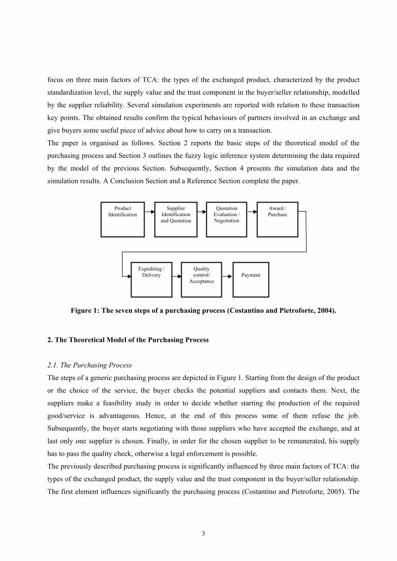
Product Identification

Supplier Identification and Quotation

Quotation Evaluation / Negotiation

Award / Purchase

Expediting / Delivery

Payment

Quality control/

Acceptance

Figure 1: The seven steps of a purchasing process (Costantino and Pietroforte, 2004).

2. The Theoretical Model of the Purchasing Process

2.1. The Purchasing Process

The steps of a generic purchasing process are depicted in Figure 1. Starting from the design of the product

or the choice of the service, the buyer checks the potential suppliers and contacts them. Next, the

suppliers make a feasibility study in order to decide whether starting the production of the required

good/service is advantageous. Hence, at the end of this process some of them refuse the job.

Subsequently, the buyer starts negotiating with those suppliers who have accepted the exchange, and at

last only one supplier is chosen. Finally, in order for the chosen supplier to be remunerated, his supply

has to pass the quality check, otherwise a legal enforcement is possible.

The previously described purchasing process is significantly influenced by three main factors of TCA: the

types of the exchanged product, the supply value and the trust component in the buyer/seller relationship.

The first element influences significantly the purchasing process (Costantino and Pietroforte, 2005). The

3

purchasing process of a highly standardized product (e.g. basic materials or standard components) is

usually characterized by:

a) a small amount of information flows with high codification levels;

b) a reduced risk of contractual hazards (because of the small amount of exchanged information and its

highly codified nature) and, therefore, of opportunistic behaviour.

On the contrary, the purchasing process of a product with low standardization level is characterized by:

a) a large amount of information flows with varying extents of customization;

b) a higher risk of contractual hazards and opportunistic behaviour (because of its low level of

standardization).

This situation leads to the persistence of using proven and known suppliers, independently from the

possible advantages of shared idiolects.

Hence, the two types of products lead to significantly different purchasing processes.

Moreover, products with different supply values clearly lead to different levels of attention in the buying

process, and then different transaction costs. More precisely, a low supply value leads to lower values of

the connected transaction costs, whereas a high supply value involves higher costs of such a kind.

The third element differentiating the purchasing process is strictly connected to the buyer/seller

relationship, that is characterised by different types of trust. Sako (1992) focuses on three types of trust:

1) contractual trust, i.e. trust in that the other party will execute the contract; 2) competence trust, i.e.

trust in that the other party is competent; 3) goodwill trust, i.e. trust in that the other party is committed to

the relationship and will do, whenever possible, more than what is specified in the contract. Both

contractual and competence trust are necessary to carry out any buyer/seller relationship. What really

distinguishes a co-operative relationship from a competitive one is that the former depends on and is

sustained by the existence of goodwill trust, which is not present in the latter form of relationship.

2.2. The Probabilistic Model of Purchasing Price and Transaction Costs

The probabilistic model evaluating the total costs of a transaction is based on an approach previously

proposed by some of the authors in Costantino et al., 2005. In the following we briefly describe the

statistical distributions used in the revisited model to quantify the expected costs for the supply, starting

from the purchasing price. In particular, it is assumed that the probability distribution of the purchasing

price is Gaussian and may thus be characterized by an average value (which is the price expected by the

buyer) and a standard deviation (because the offered price varies from a supplier to another): obviously,

such parameters are significantly different for a standardized or customized product. The choice of a

Gauss distribution is motivated by the fact that the technologies used by different suppliers and the

dimension of each of these can affect, even significantly, the charged purchasing prices. Obviously, the

4

standard deviation for a standardized product is lower than the one associated with a customized good:

indeed, the possibility to obtain different prices for the former type of product is lower than for the latter.

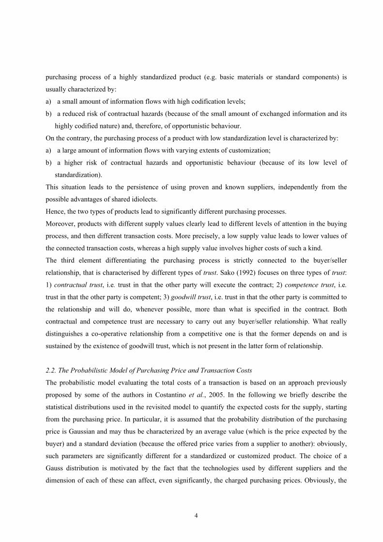
Figure 2 shows two examples of the probability distribution of the purchasing price for two products,

corresponding to the expression: 2

2( )

21( )2

−µ−

σ=πσ

PP

PP P e , (1)

where µ and σ are the average value and the standard deviation of the considered distribution,

respectively, PP represents the purchasing price in Euros and P(PP) is its probability value. Note that in

Figure 2 the values µ1=µ2=25,000 Euros, σ1=500 Euros and σ2=2,500 Euros are chosen, where the

pedices 1 and 2 obviously refer to the two different products. Hence, in the considered cases the first

product is labelled commodity product, while the second good is indicated as an asset specific product

(compare the values of σ1 and σ2 and the distributions depicted in Figure 2).

1.5 2 2.5 3 3.5

x 104

0

1

2

3

4

5

6

7

8

x 10-4

Purchasing Price (Euros)

Prob

abili

ty

Commodity ProductAsset Specific ProductAverage value

µ

Figure 2: The purchasing price distribution for two different

kinds of products sharing the same average expected price.

According to the theory first proposed by Coase (1937) and subsequently extended by Buvik (2002), the

model proposed in Costantino et al., 2005 classifies the transaction costs into ex ante and ex post costs. In

particular, ex ante costs are composed by:

1) the costs of research of suppliers CR;

2) the negotiation costs CN with the suppliers that are able to supply the product;

3) the costs of drafting and approval of the contract CDA with the supplier that has proposed the best

5

price, considering also the buyer’s preference rate, defined in the sequel, that varies from a supplier to

another.

In addition, ex post costs are divided into:

1) the quality control costs CQ;

2) the enforcement costs CE.

Ex ante costs are expressed taking into account the time of the buyer and his hour cost and are

deterministic in nature (since the times of research, contact, negotiation, drafting and approval of the

contract depend only on the kind of product and the relationship with the supplier). Furthermore, quality

control costs are considered as a function of the time of the quality department employee and his hour

cost. In addition, enforcement costs are expressed as proportional to the time of the lawyer and his hour

cost. Hence, ex post costs exhibit probabilistic distributions for control and enforcement times (due to the

significant variations of quality control and enforcement time from a supply to another).

Accordingly, research and contact costs are expressed as follows:

1(

== +∑ i i

s)R A R C

iC c t t , (2)

where s is the number of consulted suppliers, cA represents the hour cost of the buyer, and tRi and tCi

represent respectively the research time and the contact time for the generic i-th supplier.

Moreover, negotiation costs may be expressed as follows:

1== ∑ i

aN A N

iC c t , (3)

where a is the number of suppliers that are able to supply the new product/service and tNi is the

negotiation time for the generic i-th supplier.

In addition, the costs of drafting and approval of the contract with the chosen supplier are:

=DA A DAC c t (4)

with tDA representing the time of approval and drafting of the contract.

As regards the quality control costs, if cQ is the hour cost of the quality department employee and tQ

represents the control time for the supply, then such costs may be determined as follows:

=Q Q QC c t . (5)

Analogously, the enforcement costs are:

=E E EC c t , (6)

where cE indicates the hour cost of the lawyer and tE is the enforcement time.

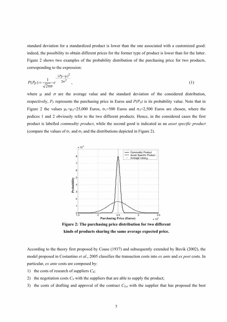
In particular, we assume that the quality control time is modelled by a Beta distribution, while an

exponential distribution is preferred for the enforcement time. Indeed, the Beta distribution fits very well

6

quality control costs because it presents a zero probability of a zero control time, a high probability of a

low control time and a decreasing probability of a high control time. In addition, the exponential

distribution is extremely suitable to model enforcement costs, since, starting from zero, the enforcement

time increases as the probability density decreases. The two described distributions are characterized as

follows. The Beta distribution is expressed as:

2 1111 11

1 21 2 0

1( ) (1 ) where ( , ) (1 )( , )

− −−= − = −∫b bb

Q Q QP T T T B b b x x dxB b b

2 1−b , (7)

where TQ=tQ/tQmax is the normalized control time, P(TQ) is its probability value, tQmax is the quality control

time maximum value for the selected supplier and b1 and b2 are the distribution characteristic parameters.

In addition, the exponential distribution is expressed by:

1( )−

µ=µ

EE

t

EE

P t e (8)

where P(tE) is the enforcement time probability value and µE is the average value for the enforcement

time.

The two distributions expressed by equations (7) and (8) are depicted in Figures 3a and 3b, respectively.

Note that in the depicted cases the values b1=2, b2=8 and µE=3h are chosen.

Finally, the transaction costs CT are the summation of the previously mentioned costs, i.e. it holds:

= + + + +T R N DA QC C C C C CE . (9)

0 0.1 0.2 0.3 0.4 0.5 0.6 0.7 0.8 0.9 10

0.5

1

1.5

2

2.5

3

3.5

4

Normalized Quality Control Time

Prob

abili

ty

0 1 2 3 4 5 6 7 8 9 100

0.05

0.1

0.15

0.2

0.25

0.3

0.35

0.4

0.45

0.5

Enforcement Time (h)

Prob

abili

ty

(a) (b)

Figure 3: The Beta probability distribution (a) and the exponential one (b) of the model.

2.3. The Theoretical Model of the Transaction

7

The theoretical model of the transaction is composed of several steps, that are summarised in the flow

chart depicted in Figure 4. In particular, according to the previously introduced estimates of the

purchasing price and transaction costs, the flow chart in Figure 4 shows all the considered hierarchical

levels in order to calculate the total costs of a supply. More precisely, the model starts with the buyer

choosing the number s of suppliers to be consulted, so that it is possible to determine the research and

contact costs CR according to (2). Subsequently, the five steps that are briefly outlined in the sequel are

executed.

From now on, only one supplier

Total costs Calculation of the total costs

Step 4 : determining the control time Quality tests Calculation of the

quality control costs

Step 5 : determining the enforcement

timeEnforcement Calculation of the

enforcement costs

a suppliers able to supply the product/service

Calculation of the negotiation costs

Calculation of drafting costs and

approval of the contract

Step 3 : determining the probability to draft and approve

the contract

Research of s suppliers Calculation of the research costs

Step1: determining capable suppliers

Purchasing price/ choice of supplier

Evaluating the Lowest Purchasing Price

Step 2 : determining the purchasing price via the Gauss distribution and preference rate

Agreement?No

Yes

FIS2FIS3 FIS1

FIS4

FIS5

FIS6

Figure 4: The flow chart of the proposed theoretical model.

Step 1. Identify the suppliers involved in the exchange and determine the negotiation costs. This step

evaluates the number a≤s of suppliers, among the s consulted ones, that are able to supply the required

product/service. Such a number is determined by simulating the feasibility study made by the i-th supplier

for i=1,…,s via a uniform probability pi of success assigned by the expert to each seller and indicating the

probability that the supplier will accept to take part in the exchange. Obviously, the success probability is

strictly connected both to the buyer/seller relationship and to the reliability of the considered supplier, as

well as to contingent phenomena, such as strikes, supplier workloads etc. Hence, the success probability

belongs to the experience of the buyer or the logistics employee.

Having identified the suppliers available for the transaction, it is now possible to determine the

8

negotiation costs CN according to (3).

Step 2. Determine the purchasing price. In this step, the Gauss distribution described by equation (1) is

employed in order to determine the probability distribution of all the offers of the different suppliers. In

particular, the model chooses at random a purchasing prices from the distribution just mentioned. Next,

the prices are compared considering the preference rate γ, defined as the percentage of the purchasing

price that the buyer is willing to pay more in order to obtain the supply from a certain supplier. This rate

may change from a supplier to another: for instance, for some supplier it may hold γ=0, which models the

circumstance that the buyer has no preference for such a provider (e.g. the latter has never participated to

a transaction with the purchaser). Finally, the chosen supplier is determined as the one exhibiting the

Lowest Purchasing Price (LPP), defined as follows:

1,..,min [ (1 )]=

= iP ii a

LPP P − γ , (10)

where PPi is the generic purchasing price which is associated to the preference rate γi for the i-th supplier.

Step 3. Determine the costs of drafting and approval of the contract. Once the negotiating is finished and

only one supplier is chosen, it is necessary to determine the probability to draft and approve the contract.

Hence, we introduce a uniform probability PS of success in drafting and approving the contract, a

parameter that may depend on the reliability of the supplier. In case the agreement is not reached, a new

number a of suppliers among the consulted s is determined: obviously, in such a case the product costs

increase, because the costs already paid for the failed contract (i.e. the research and the negotiation costs)

have to be added to the new ones in order to determine the total price of the requested product/service.

Finally, the costs of drafting and approval of the contract CDA are calculated according to (4).

Step 4. Determine the quality control costs. This step implements the probability distribution of the

control time, i.e., the Beta distribution defined by (7). Then a control time is chosen at random, so that it

is possible to determine the quality control costs CQ according to (5).

Step 5. Determine the enforcement costs. This last step determines, in an analogous way to the previous

one, the enforcement costs, that complete the transaction costs. In particular, the probability distribution

of the enforcement time, i.e., the exponential distribution expressed by (8), is considered. Then an

enforcement time is chosen at random to determine the enforcement costs CE according to (6).

Once all the ex ante and ex post costs are known, it is possible to determine the transaction costs by

9

adding them according to (9). Finally, such transaction costs are added to the purchasing price obtained in

Step 2 and corresponding to the chosen supplier, in order to determine the total costs associated with the

transaction.

The described theoretical model of the transaction requires as inputs several data, related to the particular

buyer/seller relationship, that are synthetically represented by blocks FIS1 to FIS6 in Figure 4. The next

Section shows how fuzzy logic based reasoning may be employed in order to determine these inputs to

the transaction model.

3. The Fuzzy Logic Inference System

The theoretical model for the purchasing price and the transaction costs described in the previous Section

is based on the evaluation of ex ante and ex post costs. Both such costs categories require the

quantification of several data related to the buyer operating the transaction. In particular, some parameters

characterizing the exchange are deterministic and known by the buyer or may be estimated on the basis of

expert advice. These are listed in the sequel:

• the number of suppliers to be consulted s;

• the average purchasing price µ;

• the maximum acceptable standard deviation of the purchasing price σmax;

• the maximum preference rate γmax;

• the standardization level of the required product SL, expressed as the 0÷1 degree of

customization. In particular, 0 corresponds to a totally customized product, 1 to a completely

standardized good and all the other values correspond to products in between;

• the supply value SV, expressed as the 0÷1 economic importance of the supply for the specific

firm. Obviously, a value close to 0 is typical of a low supply value, while a value close to 1 is

typical of a high supply value;

• the supplier reliability R, expressed as the 0÷1 degree of reliability. In particular, 0 corresponds to

a totally unreliable supplier, e.g. a new one, 1 to a completely reliable contractor, e.g. a well-

known one, and all the other values correspond to providers with characteristics in between1;

• the success probability that a consulted supplier is available to bid for the product p;

• the probability of agreement with a supplier Ps;

• the hour costs cA, cE and cC;

• the characteristic parameter b1 of the control time binomial distribution, that determines the

particular shape of the distribution and hence its appropriateness in modelling the control time

1 Such a concept of reliability is a synthesis of the three trusts quoted by Sako (1992).

10

phenomenon;

• all the maximum acceptable values of the time parameters connected to the transaction, i.e. the

maximum research and contact times tRmax and tCmax, the maximum negotiation time tNmax, the

maximum time for drafting and approving the contract tDAmax, the maximum quality control times

tQmax0 and tQmax1 for the limit cases SV=0 and SV=1 and finally the maximum enforcement time

tEmax.

On the contrary, several other parameters descriptive of the exchange are significantly influenced from

the uncertainty characterizing the transaction and are therefore subjective with respect to the buyer/seller

specific relationship. These are the following:

• the standard deviation of the purchasing price σ;

• the degree of preference of a supplier γ;

• all the time parameters connected to the transaction, i.e. the research and contact times tR and tC,

the negotiation time tN, the time for drafting and approving the contract tDA, the quality control

time tQ and finally the enforcement time tE.

Hence, in order to correctly simulate the behaviour of the buyer, some interviews with logistic and

purchasing managers, belonging to different fields, were required. Starting from such expert judgments,

in this section we propose to employ fuzzy logic in order to synthesise the subjective data required for the

transaction model. Indeed, fuzzy logic provides a natural framework to incorporate qualitative knowledge

with quantitative information such as real data. Therefore, fuzzy reasoning is particularly suitable for

determining, on the basis of the subjective and qualitative knowledge provided by the interviewed

experts, the subjective transaction costs parameters required as an input to the simulation model described

in the previous section. To this aim, a Fuzzy logic Inference System (FIS) is designed, composed of six

different fuzzy systems, indicated in the sequel by FIS1 to FIS6.

Component FIS1 addresses the problem of determining the standard deviation of the purchasing price,

normalised in the 0÷1 range, Σ on the basis of the standardization level of the required product SL by

using quantitative rules. In particular, FIS1 employs two simple qualitative rules, depicted in Table 1, that

evaluate the normalised standard deviation Σ in the 0÷1 range by way of the input variable SL. For the

sake of simplicity, the membership functions for variables SL and Σ of FIS1 are triangular and cross

vertically at a 0.5 degree of membership (completeness level). In particular, the membership functions of

the fuzzy sets Low (L) and High (H) describing the corresponding input and output variables are

represented in Figures 5 and 6a, respectively. Hence, the resulting value of the standard deviation of the

purchasing price

maxσ = Σ ⋅σ (11)

11

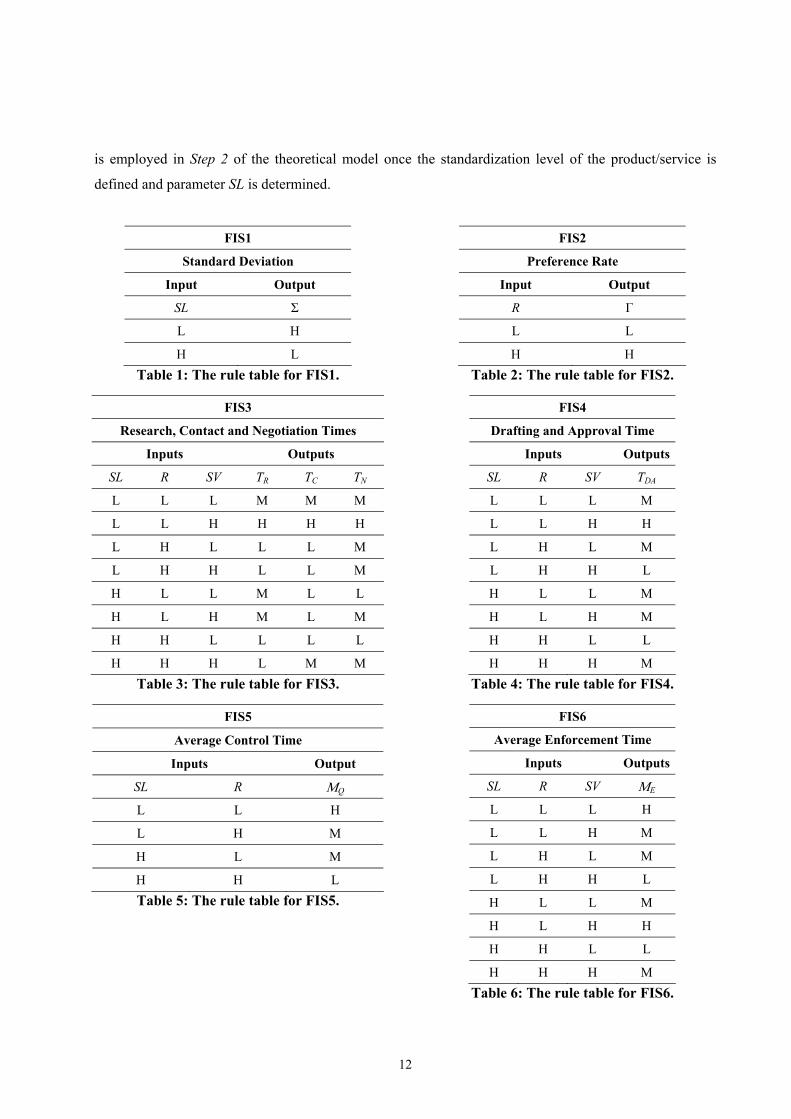
is employed in Step 2 of the theoretical model once the standardization level of the product/service is

defined and parameter SL is determined.

FIS1

Standard Deviation

Input Output

SL Σ

L H

H L Table 1: The rule table for FIS1.

FIS3

Research, Contact and Negotiation Times

Inputs Outputs

SL R SV TR TC TN

L L L M M M

L L H H H H

L H L L L M

L H H L L M

H L L M L L

H L H M L M

H H L L L L

H H H L M M Table 3: The rule table for FIS3.

FIS5

Average Control Time

Inputs Output

SL R ΜQ

L L H

L H M

H L M

H H L Table 5: The rule table for FIS5.

FIS2

Preference Rate

Input Output

R Γ

L L

H H Table 2: The rule table for FIS2.

FIS4

Drafting and Approval Time

Inputs Outputs

SL R SV TDA

L L L M

L L H H

L H L M

L H H L

H L L M

H L H M

H H L L

H H H M Table 4: The rule table for FIS4.

FIS6

Average Enforcement Time

Inputs Outputs

SL R SV ΜE

L L L H

L L H M

L H L M

L H H L

H L L M

H L H H

H H L L

H H H M Table 6: The rule table for FIS6.

12

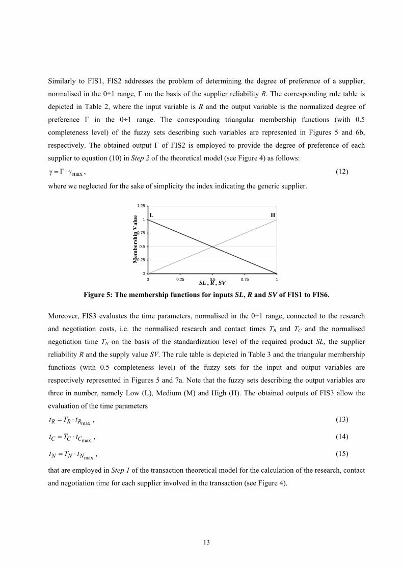
Similarly to FIS1, FIS2 addresses the problem of determining the degree of preference of a supplier,

normalised in the 0÷1 range, Γ on the basis of the supplier reliability R. The corresponding rule table is

depicted in Table 2, where the input variable is R and the output variable is the normalized degree of

preference Γ in the 0÷1 range. The corresponding triangular membership functions (with 0.5

completeness level) of the fuzzy sets describing such variables are represented in Figures 5 and 6b,

respectively. The obtained output Γ of FIS2 is employed to provide the degree of preference of each

supplier to equation (10) in Step 2 of the theoretical model (see Figure 4) as follows:

maxγ = Γ ⋅ γ , (12)

where we neglected for the sake of simplicity the index indicating the generic supplier.

0

0.25

0.5

0.75

1

1.25

0 0.25 0.5 0.75 1SL , R , SV

Mem

bers

hip

Val

ue

L H

Figure 5: The membership functions for inputs SL, R and SV of FIS1 to FIS6.

Moreover, FIS3 evaluates the time parameters, normalised in the 0÷1 range, connected to the research

and negotiation costs, i.e. the normalised research and contact times TR and TC and the normalised

negotiation time TN on the basis of the standardization level of the required product SL, the supplier

reliability R and the supply value SV. The rule table is depicted in Table 3 and the triangular membership

functions (with 0.5 completeness level) of the fuzzy sets for the input and output variables are

respectively represented in Figures 5 and 7a. Note that the fuzzy sets describing the output variables are

three in number, namely Low (L), Medium (M) and High (H). The obtained outputs of FIS3 allow the

evaluation of the time parameters

max= ⋅R R Rt T t , (13)

max= ⋅C C Ct T t , (14)

max= ⋅N N Nt T t , (15)

that are employed in Step 1 of the transaction theoretical model for the calculation of the research, contact

and negotiation time for each supplier involved in the transaction (see Figure 4).

13

0

0,25

0,5

0,75

1

1,25

0 0,25 0,5 0,75 1Σ

Mem

bers

hip

Val

ue L H

0

0,25

0,5

0,75

1

1,25

0 0,25 0,5 0,75 1Γ

Mem

bers

hip

Val

ue L H

(a) (b)

Figure 6: The membership functions for outputs Σ of FIS1 (a) and Γ of FIS2 (b).

0

0.25

0.5

0.75

1

1.25

0 0.25 0.5 0.75 1T R , T C , T N

Mem

bers

hip

Val

ue L HM

0

0.25

0.5

0.75

1

1.25

0 0.25 0.5 0.75 1T DA

Mem

bers

hip

Val

ueL HM

(a) (b)

Figure 7: The membership functions for outputs TR, TC and TN of FIS3 (a) and TDA of FIS4 (b).

0

0.25

0.5

0.75

1

1.25

0 0.25 0.5 0.75 1M Q

Mem

bers

hip

Val

ue L HM

0

0.25

0.5

0.75

1

1.25

0 0.25 0.5 0.75 1M E

Mem

bers

hip

Val

ue L HM

(a) (b)

Figure 8: The membership functions for outputs MQ of FIS5 (a) and ME of FIS6 (b).

In addition, component FIS4 evaluates the drafting and approval of the contract time parameter,

normalised in the 0÷1 range, TDA. This is determined on the basis of the standardization level of the

required product SL, the supplier reliability R and the supply value SV . The rule table is depicted in Table

4 and the triangular membership functions (with 0.5 completeness level) of the fuzzy sets for the

corresponding input and output variables are respectively represented in Figures 5 and 7b. Obviously, the

14

obtained output of FIS4 is employed in Step 3 of the transaction model for the calculation of the drafting

and approval of the contract time for the selected supplier (see Figure 4) as follows:

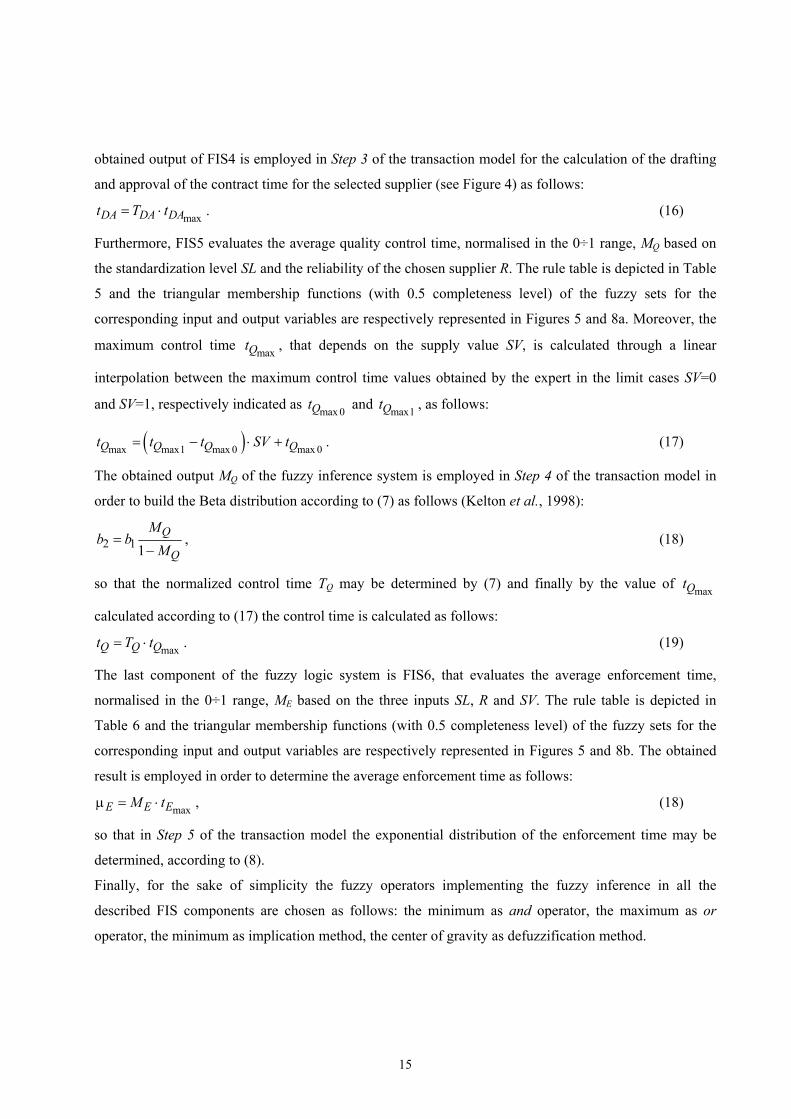
max= ⋅DA DA DAt T t . (16)

Furthermore, FIS5 evaluates the average quality control time, normalised in the 0÷1 range, MQ based on

the standardization level SL and the reliability of the chosen supplier R. The rule table is depicted in Table

5 and the triangular membership functions (with 0.5 completeness level) of the fuzzy sets for the

corresponding input and output variables are respectively represented in Figures 5 and 8a. Moreover, the

maximum control time , that depends on the supply value SV, is calculated through a linear

interpolation between the maximum control time values obtained by the expert in the limit cases SV=0

and SV=1, respectively indicated as and , as follows:

maxQt

max 0Qt max1Qt

( )max max1 max 0 max 0= − ⋅ +Q Q Q Qt t t SV t . (17)

The obtained output MQ of the fuzzy inference system is employed in Step 4 of the transaction model in

order to build the Beta distribution according to (7) as follows (Kelton et al., 1998):

2 1 1=

−Q

Q

Mb b

M, (18)

so that the normalized control time TQ may be determined by (7) and finally by the value of

calculated according to (17) the control time is calculated as follows:

maxQt

max= ⋅Q Q Qt T t . (19)

The last component of the fuzzy logic system is FIS6, that evaluates the average enforcement time,

normalised in the 0÷1 range, ME based on the three inputs SL, R and SV. The rule table is depicted in

Table 6 and the triangular membership functions (with 0.5 completeness level) of the fuzzy sets for the

corresponding input and output variables are respectively represented in Figures 5 and 8b. The obtained

result is employed in order to determine the average enforcement time as follows:

maxµ = ⋅E E EM t , (18)

so that in Step 5 of the transaction model the exponential distribution of the enforcement time may be

determined, according to (8).

Finally, for the sake of simplicity the fuzzy operators implementing the fuzzy inference in all the

described FIS components are chosen as follows: the minimum as and operator, the maximum as or

operator, the minimum as implication method, the center of gravity as defuzzification method.

15

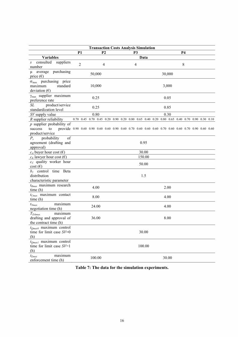
Transaction Costs Analysis Simulation P1 P2 P3 P4

Variables Data s consulted suppliers number 2 4 4 8

µ average purchasing price (€) 50,000 30,000

σmax purchasing price maximum standard deviation (€)

10,000 3,000

γmax supplier maximum preference rate 0.25 0.05

SL product/service standardization level 0.25 0.85

SV supply value 0.80 0.30 R supplier reliability 0.70 0.45 0.70 0.45 0.20 0.90 0.20 0.80 0.65 0.40 0.20 0.80 0.65 0.40 0.70 0.90 0.30 0.10p supplier probability of success to provide product/service

0.90 0.60 0.90 0.60 0.60 0.90 0.60 0.70 0.60 0.60 0.60 0.70 0.60 0.60 0.70 0.90 0.60 0.60

Ps probability of agreement (drafting and approval)

0.95

cA buyer hour cost (€) 30.00 cE lawyer hour cost (€) 150.00 cC quality worker hour cost (€) 50.00

b1 control time Beta distribution characteristic parameter

1.5

tRmax maximum research time (h) 4.00 2.00

tCmax maximum contact time (h) 8.00 4.00

tNmax maximum negotiation time (h) 24.00 4.00

TDAmax maximum drafting and approval of the contract time (h)

36.00 8.00

tQmax0 maximum control time for limit case SV=0 (h)

30.00

tQmax1 maximum control time for limit case SV=1 (h)

100.00

tEmax maximum enforcement time (h) 100.00 30.00

Table 7: The data for the simulation experiments.

16

4. The Simulation Experiments and Results

4.1 The Simulation Specification

The theoretical model is synthesized in the software Arena (Kelton et al., 1998). We evaluate the model

by simulating several transactions on the basis of data obtained by interviews with a buyer of an industrial

company. In particular, the model is tested by means of four experiments, labelled by P1 to P4: the first

two simulations are devoted to analyze products with a higher average purchasing price (in particular we

select µ1=µ2=50,000 €); the remaining two tests analyze the purchasing of goods with a lower average

purchasing price (µ3=µ4=30,000 €). Moreover, Table 7 shows the input parameters of each simulation. For

the sake of clarity, the meaning of each parameter is repeated in the table. As an example, let us analyse

the column in Table 7 corresponding to simulation P1. In this test we consider s=2 consulted suppliers, an

average purchasing price of € 50,000 with a maximum standard deviation σmax=20% of the purchasing

price, i.e. € 10,000, a maximum preference rate for the generic supplier γmax=0.25, a standardization level

of the required product SL equal to 0.25, a supply value SV=0.80 and a reliability of the two suppliers R

equal to 0.70 and 0.45, respectively. The probability that these suppliers accept to bid is respectively 0.90

and 0.60 and the probability to reach the agreement is PS=0.95. Moreover, the considered column reports

the hour costs for the buyer cA=30 €, for the lawyer cE=150 € and for the quality control employee cC=50

€, respectively. In addition, the characteristic parameter defining the shape of the Beta distribution (7) is

b1=1.5. Finally, the maximum values of the times required to calculate the transaction costs, are the

following: tRmax=4.00 h (maximum time of research), tCmax=8.00 h (maximum time of contact), tNmax=24.00

h (maximum time of negotiation), tDAmax=36.00 h (maximum time of drafting and approval of the

contract), tQmax0=30.00 h (maximum time of quality control for the limit normalised supply value SV=0),

tQmax1=100.00 h (maximum time of quality control for the limit normalised supply value SV=1) and finally

tEmax=100.00 h (maximum time of legal enforcement).

An independent replication method is used to obtain the estimate of the total and transaction cost, with a

confidence interval of 95%. More precisely, for each simulation the cost estimates are deduced by 10,000

independent replications, so that significant results from a statistical point of view are obtained.

4.2 The Results and Discussion

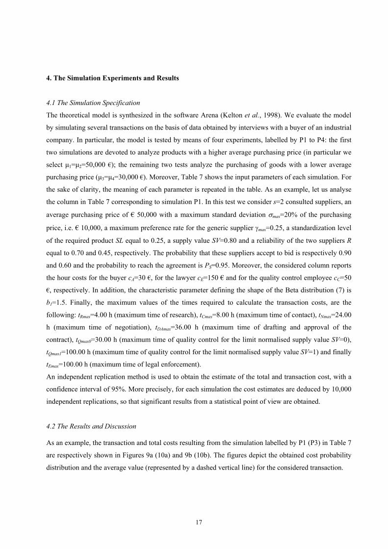
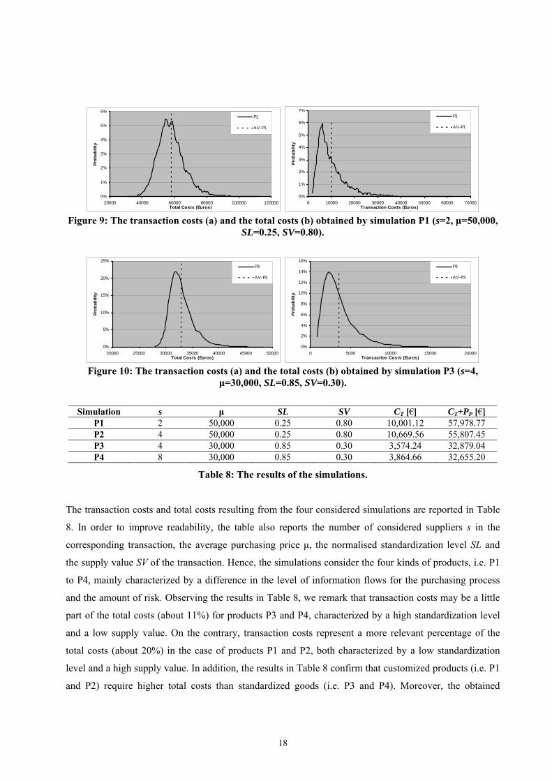
As an example, the transaction and total costs resulting from the simulation labelled by P1 (P3) in Table 7

are respectively shown in Figures 9a (10a) and 9b (10b). The figures depict the obtained cost probability

distribution and the average value (represented by a dashed vertical line) for the considered transaction.

17

0%

1%

2%

3%

4%

5%

6%

20000 40000 60000 80000 100000 120000Total Costs (Euros)

Prob

abili

ty

P1

AV-P1

0%

1%

2%

3%

4%

5%

6%

7%

0 10000 20000 30000 40000 50000 60000 70000Transaction Costs (Euros)

Prob

abili

ty

P1

AV-P1

Figure 9: The transaction costs (a) and the total costs (b) obtained by simulation P1 (s=2, µ=50,000,

SL=0.25, SV=0.80).

0%

5%

10%

15%

20%

25%

20000 25000 30000 35000 40000 45000 50000Total Costs (Euros)

Prob

abili

ty

P3

AV-P3

0%

2%

4%

6%

8%

10%

12%

14%

16%

0 5000 10000 15000 20000Transaction Costs (Euros)

Prob

abili

ty

P3

AV-P3

Figure 10: The transaction costs (a) and the total costs (b) obtained by simulation P3 (s=4,

µ=30,000, SL=0.85, SV=0.30).

Simulation s µ SL SV CT [€] CT+PP [€]

P1 2 50,000 0.25 0.80 10,001.12 57,978.77 P2 4 50,000 0.25 0.80 10,669.56 55,807.45 P3 4 30,000 0.85 0.30 3,574.24 32,879.04 P4 8 30,000 0.85 0.30 3,864.66 32,655.20

Table 8: The results of the simulations.

The transaction costs and total costs resulting from the four considered simulations are reported in Table

8. In order to improve readability, the table also reports the number of considered suppliers s in the

corresponding transaction, the average purchasing price µ, the normalised standardization level SL and

the supply value SV of the transaction. Hence, the simulations consider the four kinds of products, i.e. P1

to P4, mainly characterized by a difference in the level of information flows for the purchasing process

and the amount of risk. Observing the results in Table 8, we remark that transaction costs may be a little

part of the total costs (about 11%) for products P3 and P4, characterized by a high standardization level

and a low supply value. On the contrary, transaction costs represent a more relevant percentage of the

total costs (about 20%) in the case of products P1 and P2, both characterized by a low standardization

level and a high supply value. In addition, the results in Table 8 confirm that customized products (i.e. P1

and P2) require higher total costs than standardized goods (i.e. P3 and P4). Moreover, the obtained

18

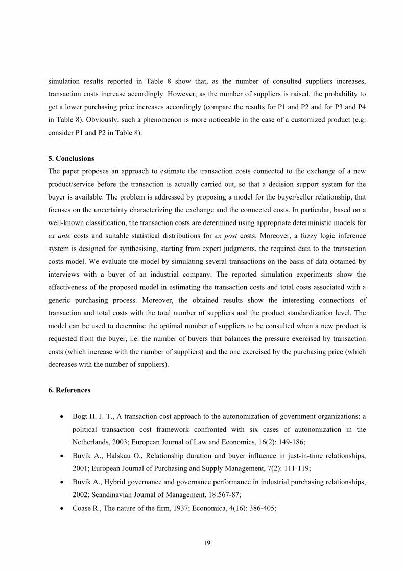
simulation results reported in Table 8 show that, as the number of consulted suppliers increases,

transaction costs increase accordingly. However, as the number of suppliers is raised, the probability to

get a lower purchasing price increases accordingly (compare the results for P1 and P2 and for P3 and P4

in Table 8). Obviously, such a phenomenon is more noticeable in the case of a customized product (e.g.

consider P1 and P2 in Table 8).

5. Conclusions

The paper proposes an approach to estimate the transaction costs connected to the exchange of a new

product/service before the transaction is actually carried out, so that a decision support system for the

buyer is available. The problem is addressed by proposing a model for the buyer/seller relationship, that

focuses on the uncertainty characterizing the exchange and the connected costs. In particular, based on a

well-known classification, the transaction costs are determined using appropriate deterministic models for

ex ante costs and suitable statistical distributions for ex post costs. Moreover, a fuzzy logic inference

system is designed for synthesising, starting from expert judgments, the required data to the transaction

costs model. We evaluate the model by simulating several transactions on the basis of data obtained by

interviews with a buyer of an industrial company. The reported simulation experiments show the

effectiveness of the proposed model in estimating the transaction costs and total costs associated with a

generic purchasing process. Moreover, the obtained results show the interesting connections of

transaction and total costs with the total number of suppliers and the product standardization level. The

model can be used to determine the optimal number of suppliers to be consulted when a new product is

requested from the buyer, i.e. the number of buyers that balances the pressure exercised by transaction

costs (which increase with the number of suppliers) and the one exercised by the purchasing price (which

decreases with the number of suppliers).

6. References

• Bogt H. J. T., A transaction cost approach to the autonomization of government organizations: a

political transaction cost framework confronted with six cases of autonomization in the

Netherlands, 2003; European Journal of Law and Economics, 16(2): 149-186;

• Buvik A., Halskau O., Relationship duration and buyer influence in just-in-time relationships,

2001; European Journal of Purchasing and Supply Management, 7(2): 111-119;

• Buvik A., Hybrid governance and governance performance in industrial purchasing relationships,

2002; Scandinavian Journal of Management, 18:567-87;

• Coase R., The nature of the firm, 1937; Economica, 4(16): 386-405;

19

• Costantino, N., Dotoli M., Falagario M., Fanti M. P., A simulation model for transaction costs in

Purchasing, 2005; Submitted for publication to Journal of Purchasing and Supply Management;

• Costantino N., Pietroforte R., Production arrangements by US building and non-building

contractors: an update, 2004; Construction Management and Economics, 22(3): 231-35;

• Costantino N., Pietroforte R., E-procurement in the construction industry: an international

comparison, 2005; CIB 2005 Conference, Helsinki: 13-16.06.2005;

• Kelton W. D., Sadowski R. P., Sadowski D. A., Simulation with Arena, 1998; Boston: Mc Graw-

Hill;

• Malone T. W., Modelling coordination in organizations and markets, 1987; Management Science,

33(10): 1317-1332;

• Masten S. J., Meehan J. W., Snyder E. E., The cost of organization, 1991; The Journal of Law,

Economics and Organization, 7(1): 1-25;

• North D., A Transaction Cost Theory of Politics, 1990; Journal of Theoretical Politics, 2(4): 355-

67;

• Rindfleisch A., Heide J. B., Transaction cost analysis: past, present and future, 1997; Journal of

Marketing, 61(4): 30-54;

• Sako M., Prices, Quality and trust: inter-firm relations in Britain and Japan, 1992; Cambridge

University Press, Cambridge;

• Shelanski H. S., Klein P. G., Empirical research in transaction cost economics: a review and

assessment, 1995; The Journal of Law, Economics and Organization, 11(2): 335-361;

• Simon H., Administrative behaviour, 1961; 2nd ed., New York: Macmillan;

• Williamson O., Markets and hierarchies: analysis and antitrust implications, 1975; New York,

NY: Free Press;

• Williamson O., The economics of organization: the transaction cost approach, 1981; American

Journal of Sociology, 87: 548-77;

• Williamson O., The economic institutions of capitalism, 1985; New York, NY: Free Press;

• Williamson O., The Mechanism of Governance, 1996; Oxford University Press.

20