Modelling the Statistics of Natural Images with ...welling/publications/papers/PoTjournal_Draft16.pdf · Modelling the Statistics of Natural Images with Topographic Product of Student-t

Modelling the Statistics of Natural Images withTopographic Product of Student-t Models

Simon Osindero

Department of Computer Science

University of Toronto

ON M5S 3G4 Canada

[email protected]

Max Welling

Department of Computer Science

University of California Irvine

CA 92697-3425 USA

[email protected]

Geoffrey E. Hinton

Canadian Institute for Advanced Research and Department of Computer Science

University of Toronto

ON M5S 3G4 Canada

[email protected]

Keywords: Energy-based model; natural scene statistics; overcomplete representations;

contrastive divergence.

Abstract

We present an energy-based model that uses a product of generalised Student-t dis-

tributions to capture the statistical structure in datasets. This model is inspired by and

particularly applicable to “natural” datasets such as images. We begin by providing

the mathematical framework, where we discuss complete as well as undercomplete

1

and overcomplete models and provide algorithms for training these models from data.

Using patches of natural scenes we demonstrate that our approach represents a viable

alternative to “independent components analysis” as an interpretive model of biolog-

ical visual systems. Although the two approaches are similar in flavor there are also

important differences, particularly when the representations are overcomplete. We

study the topographic organization of Gabor-like receptive fields that are learned by

our model, both on mono- as well as stereo-inputs. Finally, we discuss the relation of

our new approach to previous work — in particular Gaussian Scale Mixture models

and variants of independent components analysis.

1 Introduction

This paper presents a general family of energy-based models, which we refer to as “Prod-

uct of Student-t” (PoT) models, that are particularly well suited to modelling statistical

structure in data for which linear projections are expected to result in sparse marginal dis-

tributions. Many kinds of data might be expected to have such structure, and in particular

“natural” datasets such as digitised images or sounds seem to be well described in this way.

The goals of this paper are two-fold. Firstly we wish to present the general mathemat-

ical formulation of PoT models and to describe learning algorithms for such models. We

hope that this part of the paper will be useful in introducing a new method to the commu-

nity’s toolkit for machine learning and density estimation. Secondly, we focus on applying

PoT’s to capturing the statistical structure of natural scenes. This is motivated from both

a density estimation perspective, and also from the perspective of providing insight into

information processing within the visual pathways of the brain.

We suggest that the PoT model could be considered as a viable alternative to the more

familiar technique of ICA when constructing density models, performing feature extrac-

2

tion, or when building interpretive computational models of biological visual systems. As

we shall demonstrate, we are able to reproduce many of the successes of ICA — yielding

results which are comparable, but with some interesting and significant differences. Simi-

larly, extensions of our basic model can be related to some of the hierarchical forms of ICA

that have been proposed, as well as to Gaussian Scale Mixtures. Again there are interesting

differences in formulation.

The paper is organised as follows. Section 2 describes the mathematical form of the

basic PoT model along with extensions to hierarchical and topographic versions, in each

case treating representations that are complete, undercomplete and overcomplete. Section

3 then describes how to learn within the PoE framework using the contrastive divergence

(CD) algorithm (Hinton, 2002) (with Appendix A providing the background material for

running the necessary Markov Chain Monte Carlo sampling). Then in section 4 we present

results of our model when applied to natural images. We are able to recreate the success

of ICA based models (for example Bell and Sejnowski (1995, 1997); Olshausen and Field

(1996, 1997); Hoyer and Hyvarinen (2000); Hyvarinen et al. (2001); Hyvarinen and Hoyer

(2001)) in providing computationally motivated accounts for the form of simple cell and

complex cell receptive fields, as well as for the basic layout of topographic maps for loca-

tion, orientation, spatial frequency, and spatial phase. Additionally, we are easily able to

produce such results in an overcomplete setting and have made the novel contribution of

including stereoscopic properties within the same model — our preliminary results deliver

complex-cell like units with interesting disparity tuning properties and also simple topo-

graphic maps displaying ocular dominance in addition to the aforementioned properties.

In section 5 we analyse in more detail the relationships between our PoT model, ICA

models and Gaussian Scale Mixtures, and finally in section 6 we summarise our work.

3

2 Products of Student-t Models

We will begin with a brief overview of product of expert models (Hinton, 2002) in section

2.1, before presenting the basic product of Student-t model (Welling et al., 2002a) in section

2.2. Then we move on to discuss hierarchical topographic extensions in sections 2.3, 2.4

and 2.5.

2.1 Product of Expert Models

Product of expert models, or PoEs, were introduced in Hinton (2002) as an alternative

method of combining expert models into one joint model. In contrast to mixture of expert

models, where individual models are combined additively, PoEs combine expert opinions

multiplicatively as follows (see also Heskes (1998)),

PPoE(x|θ) =1

Z(θ)

M∏i=1

pi(x|θi) (1)

whereZ(θ) is the global normalization constant andpi(·) are the individual expert models.

Mixture models employ a “divide and conquer” strategy with different “experts” being used

to model different subsets of the training data. In product models, many experts cooperate

to explain each input vector and different experts specialize in different parts of the input

vector or in different types of latent structure. If a scene containsn different objects that are

processed in parallel, a mixture model needs a number of components that is exponential in

n because each component of the mixture must model acombinationof objects. A product

model, by contrast, only requires a number of components that is linear inn because many

different experts can be used at the same time.

Another benefit of product models is their ability to model sharp boundaries. In mix-

ture models, the distribution represented by the whole mixture must be vaguer than the

4

distribution represented by a typical component of the mixture. In product models, the

product distribution is typically much sharper than the distributions of the individual ex-

perts1, which is a major advantage for high dimensional data (Hinton, 2002; Welling et al.,

2002b).

Learning PoE models has been difficult in the past, mainly due to the presence of the

partition functionZ(θ). However, contrastive divergence learning (Hinton, 2002) (see

section 3.3) has opened the way to apply these models to large scale applications.

PoE models are related to many other models that have been proposed in the past. In

particular, log-linear models2 have a similar flavor, but are more limited in their parametriza-

tion:

PLogLin(x|λ) =1

Z(λ)

M∏i=1

exp

[M∑i=1

λifi(x)

](2)

whereexp[λifi(·)] takes the role of an un-normalized expert. A binary product of experts

model was first introduced under the name “harmonium” in Smolensky (1986). A learning

algorithm based on projection pursuit was proposed in Freund and Haussler (1992). In

addition to binary models (Hinton, 2002), the Gaussian case been studied (Williams et al.,

2001; Marks and Movellan, 2001; Williams and Agakov, 2002; Welling et al., 2003a).

1When multiplying togethern equal-variance Gaussians, for example, the variance is reduced by a factorof n. It is also possible to make the entropy of the product distribution higher than the entropy of the individualexperts by multiplying together two very heavy-tailed distributions whose modes are in very different places.

2Otherwise known as exponential family models, maximum entropy models and additive models.

5

2.2 Product of Student-t (PoT) Models

The basic model we study in this paper is a form of PoE suggested by Hinton and Teh

(2001) where the experts are given by generalized Student-t distributions:

y = Jx (3)

pi(yi|αi) ∝ 1

(1 + 12y2

i )αi

(4)

The variablesyi are the responses to linearly filtered input vectors and can be thought of

as latent variables that are deterministically related to the observables,x. Through this

deterministic relationship, equation 4 defines a probability density on the observables. The

filters,{Ji}, are learnt from the training data (typically images) by maximizing or approx-

imately maximizing the log likelihood.

Note that due to the presence of theJ parameters this product of Student-t (PoT) model

is not log-linear. However, it is possible to introduce auxiliary variables,u, such that the

joint distributionP (x,u) is log-linear3 and the marginal distributionP (x) reduces to that

of the original PoT distribution,

PPoT (x) =

∫ ∞

0

du P (x,u) (5)

P (x,u) ∝ exp

[−

M∑i=1

(ui

(1 +

1

2(Jix)2

)+ (1− αi) log ui

)](6)

whereJi denotes the row-vector corresponding to theith row of the filter matrixJ. The

advantage of this reformulation using auxiliary variables is that it supports an efficient, fast

mixing Gibbs sampler which is in turn beneficial for contrastive divergence learning. The

3Note that it is log-linear in the parametersθijk = JijJik andαi with featuresuixjxk andlog ui.

6

x

u

y=Jx

x

u 2

y=Jx

z=W(y)

x

u

J

W

(a) (b) (c)

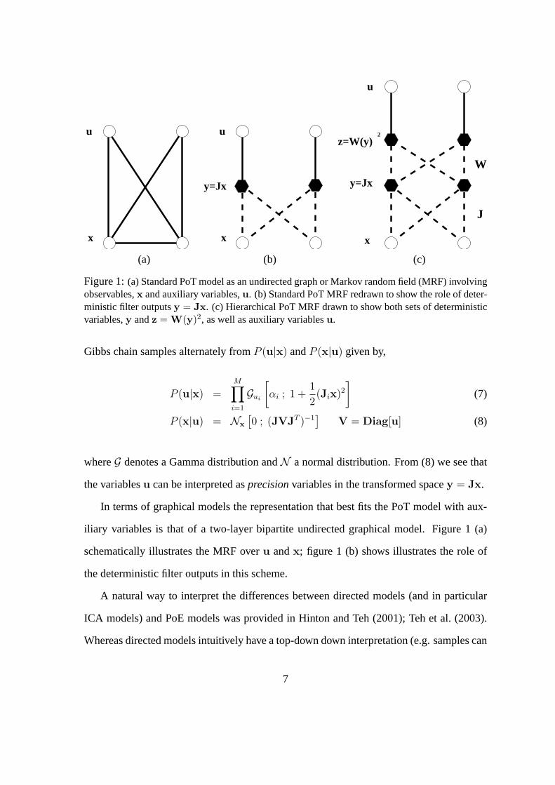
Figure 1:(a) Standard PoT model as an undirected graph or Markov random field (MRF) involvingobservables,x and auxiliary variables,u. (b) Standard PoT MRF redrawn to show the role of deter-ministic filter outputsy = Jx. (c) Hierarchical PoT MRF drawn to show both sets of deterministicvariables,y andz = W(y)2, as well as auxiliary variablesu.

Gibbs chain samples alternately fromP (u|x) andP (x|u) given by,

P (u|x) =M∏i=1

Gui

[αi ; 1 +

1

2(Jix)2

](7)

P (x|u) = Nx

[0 ; (JVJT )−1

]V = Diag[u] (8)

whereG denotes a Gamma distribution andN a normal distribution. From (8) we see that

the variablesu can be interpreted asprecisionvariables in the transformed spacey = Jx.

In terms of graphical models the representation that best fits the PoT model with aux-

iliary variables is that of a two-layer bipartite undirected graphical model. Figure 1 (a)

schematically illustrates the MRF overu andx; figure 1 (b) shows illustrates the role of

the deterministic filter outputs in this scheme.

A natural way to interpret the differences between directed models (and in particular

ICA models) and PoE models was provided in Hinton and Teh (2001); Teh et al. (2003).

Whereas directed models intuitively have a top-down down interpretation (e.g. samples can

7

be obtained by ancestral sampling starting at the top-layer units), PoE models (or more gen-

erally “energy-based models”) have a more natural bottom-up interpretation. The probabil-

ity of an input vector is proportional toexp(−E(x)) where the energyE(x) is computed

bottom-up starting at the input layer (e.g.E(y) = E(Jx)). We may thus interpret the PoE

model as modelling a collection of soft constraints, parameterized through deterministic

mappings from the input layer to the top layer (possibly parameterized as a neural network)

and where the energy serves to penalize inputs that do not satisfy these constraints (e.g. are

different from zero). The costs contributed by the violated constraints are added to com-

pute the global energy, which is equivalent to multiplying the distributions of the individual

experts to compute the product distribution (sinceP (x) ∝ ∏i pi(x) ∝ exp(−∑

i Ei(x))).

For a PoT, we have a two-layer model where the constraint-violations are penalized

using the energy function (see Eqn.6),

E(x) =M∑i=1

αi log

(1 +

1

2(Jix)2

)(9)

We note that the shape of this energy function implies that relative to a quadratic penalty,

small violations are penalized more strongly whilst large violations are penalized less

strongly. This results in “sparse” distributions of violations (y-values) with many very

small violations and occasional large ones.

In the case of equal number of observables,{xi}, and latent variables,{yi} (the so

called “complete representation”), the PoT model is formally equivalent to square, noise-

less “independent components analysis” (ICA) (Bell and Sejnowski, 1995) with Student-t

priors. However, in the overcomplete setting (more latent variables than observables) prod-

uct of experts models are essentially different from overcomplete ICA models (Lewicki

and Sejnowski, 2000). The main difference is that the PoT maintains a deterministic rela-

tionship between latent variables and observables throughy = Jx, and consequently not

8

all values ofy are allowed. This results in important marginal dependencies between the

y-variables. In contrast, in overcomplete ICA the hiddeny-variables are marginally inde-

pendent by assumption and have a stochastic relationship with thex-variables. For more

details we refer to Teh et al. (2003).

For undercomplete models (fewer latent variables than observables) there is again a

discrepancy between PoT models and ICA models. In this case the reason can be traced

back to the way noise is added to the models in order to force them to assign non-zero

probability everywhere in input space. In contrast to undercomplete ICA models where

noise is added in all directions of input space, undercomplete PoT models have noise added

only in the directions orthogonal to the subspace spanned by the filter matrixJ. More

details can be found in Welling et al. (2003b, 2004) and in section 2.3.1.

2.3 Hierarchical PoT (HPoT) Models

We now consider modifications to the basic PoT by introducing extra interactions between

the activities of filter outputs,yi, and by altering the energy function for the model. These

modifications were motivated by observations of the behaviour of ‘independent’ compo-

nents of natural data, and inspired by similarities between our model and (hierarchical)

ICA. Since the new model essentially involves adding a new layer to the standard PoT, we

refer to it as a hierarchical PoT (HPoT).

As we will show in Section 4, when trained on a large collection of natural image

patches the linear components{Ji} behave similarly to the learnt basis functions in ICA

and grow to resemble the well-known Gabor-like receptive fields of simple cells found

in the visual cortex (Bell and Sejnowski, 1997). These filters, like wavelet transforms,

are known to de-correlate input images very effectively. However, it has been observed

that higher order dependencies remain between the filter outputs{yi}. In particular there

9

are important dependencies between the “activities” or “energies”y2i (or more generally

|yi|β, β > 0) of the filter outputs. This phenomenon can be neatly demonstrated through

the use of so-called bow-tie plots, in which the conditional histogram of one filter output

is plotted given the output value of a different filter (Simoncelli, 1997) (see figure 20 for

an example). The bow-tie shape of the plots implies that the first order dependencies have

been removed by the linear filters{Ji} (the conditional mean vanishes everywhere), but

that higher order dependencies still remain; specifically, the variance of one filter output

can be predicted from the activity of neighboring filter outputs.

In our modified PoT the interactions between filter outputs will be implemented by first

squaring the filter outputs and subsequently introducing an extra layer of units, denoted

by z. These units will be used to capture the dependencies between these squared filter

outputs:z = W(y)2 = W(Jx)2, and this is illustrated in figure 1 (c). (Note that in the

previous expression, and in what follows, the use of(·)2 with a vector argument will implies

a component-wise squaring operation.)

E(x) =M∑i=1

αi log

(1 +

1

2

K∑j=1

Wij(Jjx)2

)W ≥ 0 (10)

where the non-negative parametersWij model the dependencies between the activities4

{y2i }. Note that the forward mapping fromx, throughy, to z is completely deterministic,

and can be interpreted as a bottom-up neural network. We can also view the modified PoT

as modelling constraint violations, but this time in terms ofz with violations now penalized

according to the energy in Equation 10.

As with the standard PoT model, there is a reformulation of the hierarchical PoT model

4For now, we implicitly assume that the number of first hidden-layer units (i.e. filters) is greater than orequal to the number of input dimensions. Models with fewer filters than input dimensions need some extracare. The number of top-layer units can be arbitrary, but for concreteness we will work with an equal numberof first-layer and top-layer units. For a detailed discussion see section 2.3.1.

10

in terms of auxiliary variables,u,

P (x,u) ∝ exp

[−

M∑i=1

(ui

(1 +

1

2

K∑j=1

Wij(Jjx)2

)+ (1− αi) log ui

)](11)

with conditional distributions,

P (u|x) =M∏i=1

Gui

[αi ; 1 +

1

2

K∑j=1

Wij(Jjx)2

](12)

P (x|u) = Nx

[0 ; (JVJT )−1

]V = Diag[WTu] (13)

Again, we note that this auxiliary variable representation supports an efficient Gibbs sam-

pling procedure where all auxiliary variablesu are sampled in parallel given the inputsx

using Eqn. 12 and all input variablesx are sampled jointly from a multivariate Gaussian

distribution according to Eqn.13. As we will discuss in section 3.3, this is an important

ingredient in training (H)PoT models from data using contrastive divergence.

Finally, in a somewhat speculative link to computational neuroscience, in the following

discussions we will refer to units,y, in the first hidden layer as ‘simple cells’ and units,z,

in the second hidden layer as ‘complex cells’. For simplicity, we will assume the number

of simple and complex cells to be equal. There are no obstacles to using unequal numbers,

but this does not appear to lead to any qualitatively different behaviour.

2.3.1 Undercomplete HPoT Models

The HPoT models, as defined in section 2.3, were implicitly assumed to be complete or

overcomplete. In this section we will consider undercomplete models. These models can

be interesting in a variety of applications where one seeks to represent the data in a lower

dimensional yet informative space. For instance, in computer vision applications it is often

useful to reduce the size of the representation in order to ease the computation burden on

11

later processing stages. Also, lower dimensional representations are often less “noisy” and

therefore can sometimes improve the performance of subsequent processing. One example

is “latent semantic indexing” (Deerwester et al., 1990), where the extracted latent dimen-

sions are representative of the topics in the documents in the corpus. One could imagine a

hierarchical extension of this idea where the top-layer units represent “meta-topics” which

capture information about which topics are active jointly.

Undercomplete models need a little extra care in their definition, since in the absence of

a proper noise model they are un-normalizable over input space. In Welling et al. (2003a,b,

2004) a natural solution to this dilemma was proposed where a noise model is added in

directions orthogonal to all of the filters{J}. In the following we will generalize this

procedure to the HPoT model. We start by considering the basic HPoT density iny-space:

py(y) =1

Z(W,α)exp

[−

M∑i=1

αi log

(1 +

1

2

K∑j=1

Wijy2j

)](14)

In this space we have a well defined complete product of Student-t distributions model.

The difficulty arises when we come to convert this into a well defined model overx

wherey = Jx and where the dimensionality ofx is larger than that ofy – i.e. if

we wish to perform dimensionality reduction. The reason for the difficulties lies in the

fact that entire dimensions inx-space are assigned equal probability density if we define

p(x) ∝ exp(−E(x)) by simply replacingy = Jx in Eqn.14. This implies that the proba-

bility density doesn’t decay in those directions resulting in an un-normalizable probability

density. To fix this problem we augment the originaly-space with extra dimensions by

appending the vectory⊥. The marginal distribution on the augmented space is chosen to

be an isotropic Gaussian.

p(y,y⊥) = py(y)D∏

j=M+1

Ny⊥j

[y⊥j ; 0, σ2

](15)

12

Furthermore, these extra dimensions will be assumed to be the outputs from a set of or-

thonormal filters living within the complementary subspace of the original filters,J. This

is a rather different noise model than that employed in e.g. factor analysis (Bartholomew,

1987) and probabilistic principle components analysis (Tipping and Bishop, 1999), where

noise is added in all directions of input space. In the approach we describe, Gaussian noise

is only added to the subspace orthogonal to that modelled by the filtersJ.

Finally, we need to transform this model to input space to obtain a probability den-

sity overx. Transforming a probability density between two one-to-one random variables

((y,y⊥) → x) is done by introducing a “Jacobian”,

px(x) = p(y,y⊥)

∣∣∣∣∂(y,y⊥)

∂x

∣∣∣∣ (16)

where| · | denotes the absolute value of the determinant and where(y,y⊥) is considered a

function ofx. The relation betweenx and(y,y⊥) is linear,

y = Jx (17)

y⊥ = Kx (18)

where

P⊥J = KTK = I− JT (JJT )−1J (19)

is the matrix that projects a vector inx-space onto the orthogonal complement of the space

spanned byJ. Hence the Jacobian is given by,

∣∣∣∣∂(y,y⊥)

∂x

∣∣∣∣ =

∣∣∣∣∣∣∣J

K

∣∣∣∣∣∣∣(20)

Note thatK is implicitly defined as a function ofJ. To simplify the expression for the

13

Jacobian in Eqn. 20, we use that|A| =√|AAT | for arbitrary full rank matrixA. In

particular, we will useAT = [JT |KT ] and the following two identities:

(A) JKT = KJT = 0 (21)

(B) KKT = I (22)

The first identity (A) follows because the rows ofK andJ are orthogonal by definition.

The second identity (B) follows becauseKTK is a projection operator which hasJ − D

eigenvalues1, and the rest zeros. Now assume thatu is an eigenvector ofKTK with

eigenvalue1, thenKu is an eigenvector ofKKT with eigenvalue1. Hence, all eigenvalues

of KKT are1 which implies that it must be equal toI. Using the identities (A) and (B) we

arrive at the following expression for the Jacobian,

∣∣∣∣∣∣∣J

K

∣∣∣∣∣∣∣=

√√√√√√

∣∣∣∣∣∣∣JJT JKT

KKT KKT

∣∣∣∣∣∣∣=

√√√√√√

∣∣∣∣∣∣∣JJT 0

0 I

∣∣∣∣∣∣∣=

√|JJT | (23)

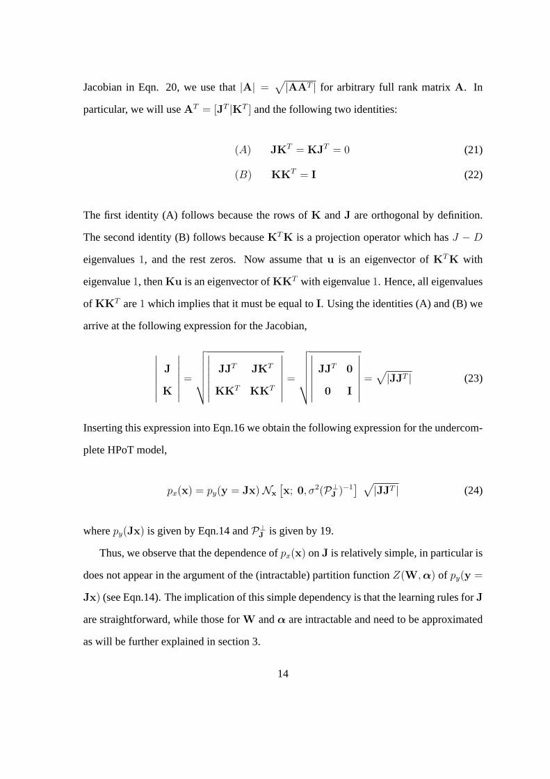
Inserting this expression into Eqn.16 we obtain the following expression for the undercom-

plete HPoT model,

px(x) = py(y = Jx) Nx

[x; 0, σ2(P⊥J )−1

] √|JJT | (24)

wherepy(Jx) is given by Eqn.14 andP⊥J is given by 19.

Thus, we observe that the dependence ofpx(x) onJ is relatively simple, in particular is

does not appear in the argument of the (intractable) partition functionZ(W,α) of py(y =

Jx) (see Eqn.14). The implication of this simple dependency is that the learning rules forJ

are straightforward, while those forW andα are intractable and need to be approximated

as will be further explained in section 3.

14

2.4 Topographic PoT Models

The modifications described next were inspired by a similar proposal in Hyvarinen et al.

(2001) named “topographic ICA”. By restricting the interactions in between the first and

second layers of a HPoT model we are able to induce a topographic ordering on the learnt

features. In addition to promoting order, this restriction should also help to regularise the

density models that we learn. Further discussion on the relationships between PoT’s and

ICA is given in Teh et al. (2003) and in section 5.

We begin by choosing a topology on the space of the filters. This is done most con-

veniently by defining aM × M neighborhood matrixF with 1’s at positions(i, j) for

filters that are considered neighbors and0’s everywhere else5. In all our experiments we

have chosen the filters to be organized on a square grid and we apply periodic (toroidal)

boundary conditions to avoid boundary effects (see figure 5).

Having established the topology of the space space in which the filters “live”, we now

consider how the learning procedure leads to their spatial organisation. The effect of our

restriction to the energy function should be such that nearby filters in the filter-map behave

similarly in a statistically sense. More precisely, the activities (squared output) of nearby

units in the first layer of our model should by highly correlated for the input ensemble

under consideration (i.e. our data). To accomplish this we define top-layer units (‘complex

cells’) that receive inputlocally from the layer below (‘simple cells’).

The complex cells receive input from the simple cells in precisely the same way as in

our HPoT model:yi =∑

j Wij(Jjx)2, but nowW is fixed and we assume it is chosen

such that it computes a localaverageof the activities. The free parameters that remain to

be learnt using contrastive divergence are{αi,J}. In the following we will explain why

the the filters{Ji} should be expected to organize themselves topographically when learnt

from data.5Units may be neighbors to themselves, i.e.1’s on the diagonal are allowed

15

As noted previously, there are important dependencies between the activities of wavelet

coefficients of filtered images. In particular, the variance (but not the mean) of one coef-

ficient can be predicted from the value of a “neighboring” coefficient. The topographic

PoT model can be interpreted as an attempt to model these dependencies through a Markov

random field on the activities of the simple cells. However, we have pre-defined the con-

nectivity pattern and have left the filters to be determined through learning. This is the

opposite strategy as the one used in, for instance, Portilla et al. (2003) where the wavelet

transform is fixed and the interactions between wavelet coefficients are modelled. One pos-

sible explanation6 for the emergent topography is that the model will make optimal use of

these pre-defined interactions if it organizes its simple cells such that dependent cells are

nearby in filter space and independent ones are distant.

A complementary explanation is based on the interpretation of the model as capturing

complex constraints in the data. The penalty function for violations is designed such that

(relative to a squared penalty) large violations are relatively mildly penalized (see figure 2).

However, since the complex cells represent the average input from simple cells, their values

would be well described by a Gaussian distribution if the corresponding simple cells were

approximately independent. (This is a consequence of the central limit theorem for sums

of independent random variables.) In order to avoid a mismatch between the distribution

of complex cell outputs and the way they are penalized, the model ought to position simple

cells that have correlated activities near to each other. In doing so, the model can escape the

central limit theorem because the simple cell outputs that are being pooled are no longer

independent. Consequently, the pattern of violations that arises is a better match to the

pattern of violations which one would expect from the penalising energy function.

Another way to understand the pressure towards topography is to ask how an individual

6The above arguments assume that the shape of the filters remains unchanged (i.e. Gabor-like) by theintroduction of the complex cells in the model. In experiments we have indeed verified that this is the case.

16

-10 -8 -6 -4 -2 0 2 4 6 8 100

0.1

0.2

0.3

0.4

0.5

0.6

0.7

0.8

0.9

1

Beta=5

Beta=2

Beta=1/2

Figure 2:Functionsf(x) = 1/(1 + |x|β) for different values ofβ.

simple cell should be connected to the complex cells in order to minimize the total cost

caused by the simple cell’s outputs on real data. If the simple cell is connected to complex

cells that already receive inputs from the simple cell’s neighbors in position and spatial

frequency, the images that cause the simple cell to make a big contribution will typically

be those in which the complex cells that it excites are already active, so its additional

contribution to the energy will be small because of the gentle slope in the heavy tails of the

cost function. Hence, since complex cells locally pool simple cells, topography is expected

to emerge.

2.5 Further Extensions To The Basic PoT Model

The parameters{αi} in the definition of the PoT model control the “sparseness” of the

activities of the complex and simple cells. For large values ofα, the PoT model will

resemble more and more a Gaussian distribution, while for small values there is a very tall

peak at zero in the distribution which decays very quickly into “fat” tails.

In the HPoT model, the complex cell activities,z, are the result of the linearly com-

bining the (squared) outputs simple cells,y = Jx. The squaring operation is a somewhat

arbitrary choice, and we may wish to process the first layer activities in other ways before

17

we combining them in the second layer. In particular, we might consider modifications of

the form: activity=|Jx|β with |·| denoting absolute values andβ > 0. Such a model defines

the a density iny-space of the form,

py(y) =1

Z(W,α)exp

[−

M∑i=1

αi log

(1 +

1

2

K∑j=1

Wij|yj|β)]

(25)

A plot of the un-normalized distributionf(x) = 1/(1 + |x|β) (i.e. withα = 1) is shown in

figure 2 for three setting of the parameterβ. One can observe that for smaller values ofβ

the peak at zero become stronger and the tails become “fatter”.

In section 3 we will show that sampling and hence learning with contrastive divergence

can be performed efficiently for any setting ofβ.

3 Learning in HPoT Models

In this section we will explain how to perform maximum likelihood learning of the pa-

rameters for the models introduced in the previous section. In the case of complete and

undercomplete PoT models we are able to analytically compute gradients, however in the

general case of overcomplete or hierarchical PoT’s we are required to employ an approxi-

mation scheme and the preferred method in this paper will be contrastive divergence (CD)

(Hinton, 2002). Since CD learning is based on Markov chain Monte Carlo sampling, Ap-

pendix A provides a discussion of sampling procedures for the various models we have

introduced.

18

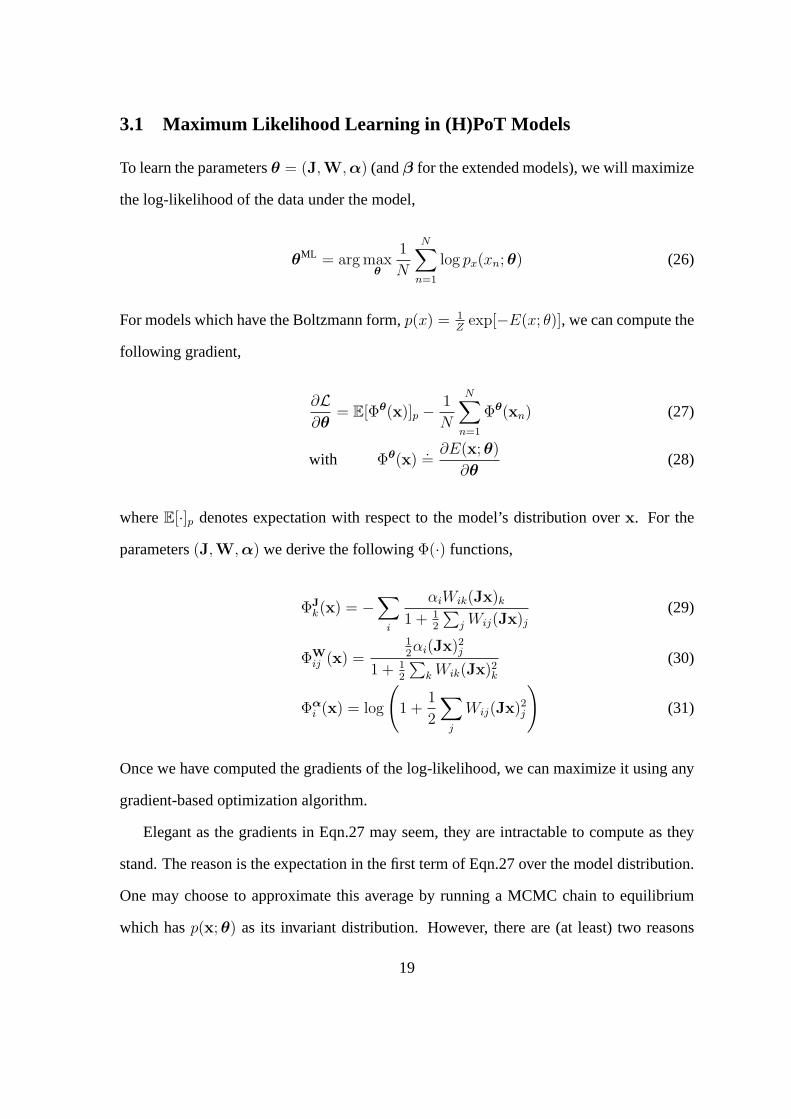
3.1 Maximum Likelihood Learning in (H)PoT Models

To learn the parametersθ = (J,W,α) (andβ for the extended models), we will maximize

the log-likelihood of the data under the model,

θML = arg maxθ

1

N

N∑n=1

log px(xn; θ) (26)

For models which have the Boltzmann form,p(x) = 1Z

exp[−E(x; θ)], we can compute the

following gradient,

∂L∂θ

= E[Φθ(x)]p − 1

N

N∑n=1

Φθ(xn) (27)

with Φθ(x).=

∂E(x; θ)

∂θ(28)

whereE[·]p denotes expectation with respect to the model’s distribution overx. For the

parameters(J,W,α) we derive the followingΦ(·) functions,

ΦJk(x) = −

∑i

αiWik(Jx)k

1 + 12

∑j Wij(Jx)j

(29)

ΦWij (x) =

12αi(Jx)2

j

1 + 12

∑k Wik(Jx)2

k

(30)

Φαi (x) = log

(1 +

1

2

∑j

Wij(Jx)2j

)(31)

Once we have computed the gradients of the log-likelihood, we can maximize it using any

gradient-based optimization algorithm.

Elegant as the gradients in Eqn.27 may seem, they are intractable to compute as they

stand. The reason is the expectation in the first term of Eqn.27 over the model distribution.

One may choose to approximate this average by running a MCMC chain to equilibrium

which hasp(x; θ) as its invariant distribution. However, there are (at least) two reasons

19

why this might not be a good idea: 1) The Markov chain has to be run to equilibrium for

every gradient step of learning and 2) we need a lot of samples to reduce the variance in

the estimates.

Hence, for the general case, we propose to use the contrastive divergence learning

paradigm which is discussed in section 3.3. In a few special cases we can actually find

analytic expressions for the gradients, which we will discuss next.

3.2 Maximum Likelihood Learning for Complete and Undercomplete

(H)PoT Models

For complete and undercomplete HPoT models we can derive the exact gradient of the log-

likelihood w.r.t the parametersJ. The reason is that the partition functionZ(W,α) does

not depend onJ as explained in section 2.3.1. Since complete models are a special case of

the undercomplete models (withM = D), we focus on the latter and comment on how the

gradients simplify when we consider the former. Using the probability density of Eqn.24,

we arrive at the following derivatives,

∂L∂J

= J#T +1

σ2J#TCP⊥J +

1

N

N∑n=1

Φ(Jxn)xTn (32)

with J# = JT (JJT )−1 (the pseudo-inverse) andC = 1N

∑Nn=1 xnx

Tn . We have also used

the fact that,12∂ log

∣∣JJT∣∣ /∂J = J#T . The maximum likelihood solution for the noise

varianceσ2 is simply given by the average variance in the directions orthogonal to the

subspace spanned byJ,

σ2 =tr(CP⊥J )

D −M(33)

If we assume that the data has been sphered in a preprocessing step we immediately see

that the second term in Eqn.32 vanishes sinceC = I andJ#TP⊥J = 0. Also,σ = 1 in that

20

case.

WhenM = D (i.e. the complete case) the second term also vanishes and in addition

we can also useJ# = J−1 in Eqn.32. This is in fact the general update rule for the

ICA algorithm proposed in Bell and Sejnowski (1995), using Student-t distributions for the

sources.

Learning the parametersW,α is much harder, because the partition function depends

on both of them. However, in the special case where we setW = I (i.e. the non-

hierarchical PoT model), learningα can be performed analytically because the joint model

in z-space factors intoM componentspz(z) =∏

i pzi(zi), with

pi(zi) =Γ(αi)

Γ(αi − 12)√

2π

(1 +

1

2z2

i

)−αi

(34)

The learning rule is given by,

∂L∂αi

= Ψ(αi)−Ψ(αi − 1

2)− 1

N

N∑n=1

log

(1 +

1

2(Jxn)2

i

)(35)

whereΨ(·) is the digamma function which represents the derivative ofln Γ(·).

3.3 Training (H)PoT Models with Contrastive Divergence

In the previous section we discussed some special cases in which the gradients of the log-

likelihood can be computed analytically. In this section we will describe an approximate

learning paradigm to train the parameters in cases where evaluation of the exact gradients

is intractable. Recall that the bottleneck in computing the exact gradients is the first term in

the expressions 29, 30 and 31. An approximation to these expressions can be obtained by

running a MCMC sampler withp(x;J,W, α) as its invariant distribution and computing

Monte Carlo estimates of the averages. As mentioned in section 3.2 this is a very ineffi-

21

cient procedure because it needs to be repeated for every step of learning and a fairly large

number of samples may be needed to reduce the variance in the estimates7. Contrastive di-

vergence (Hinton, 2002), replaces the MCMC samples in these Monte Carlo estimates with

samples from brief MCMC runs, which were initialized at the data-cases. The intuition is

that if the current model is not a good fit for the data, the MCMC particles will swiftly and

consistently move away from the data cases. On the other hand, if the data population rep-

resents a fair sample from the model distribution, then the average energy will not change

when we initialize our Markov chains at the data cases and run them forward. In general,

initializing the Markov chains at the data and running them only briefly introduces bias but

greatly reduces both variance and computational cost.Algorithm 1 summarise the steps in

this learning procedure.

Algorithm 1 Contrastive Divergence Learning

1. Compute the gradient of the energy with respect to the parameters,θ, and average overthe data casesxn.

2. Run MCMC samplers fork steps, starting at every data vectorxn, keeping only thelast samplesn,k of each chain.

3. Compute the gradient of the energy with respect to the parameters,θ, and average overthe samplessn,k.

4. Update the parameters using,

∆θ =η

N

∑

samplessn,k

∂E(snk)

∂θ−

∑dataxn

∂E(xn)

∂θ

(36)

whereη is the learning rate andN the number of samples in each mini-batch.

For further details on contrastive divergence learning we refer to the literature (Hinton,

2002; Teh et al., 2003; Yuille, 2004; Carreira-Perpinan and Hinton, 2005). For highly

overcomplete models it often happens that some of theJi-filters (rows ofJ) decay to

zero. To prevent this from happening we constrain theL2-norm of these filters to be one:

7An additional complication is that it is hard to assess when the Markov chain has converged to theequilibrium distribution.

22

∑j J2

ij = 1 ∀i. Also, constraining the norm of the rows of theW matrix was helpful during

learning. We choose to constrain theL1 norm to unity∑

j Wij = 1 ∀i, which makes sense

becauseW ≥ 0.

Figure 3: A random sample of144 out of 361 learnt filters for the CEDAR digits. Each

square shows the weights of one filter. The scale that relates filter weights to gray levels

in the figure is different for each filter and is chosen to make use of the full range of gray

levels. Also, to make it easier to discern the structure of the learnt filters, we present them

in the ZCA whitened domain rather than in raw pixel space.

3.4 An Illustrative Example

Before proceeding to discuss PoT’s applied to natural images we present a simple exam-

ple of unsupervised feature extraction to give a flavour for PoT models. In addition to

describing the probability density of a dataset, models such as ours can often yield useful

and interpretable “features” of the data. These features are well motivated by the statistical

23

structure of the data upon which they are trained, so we might expect them to be useful

for a range of tasks. For instance, one might explore their use in classification or data

visualisation tasks.

We used the digit set of size16×16 real values from the “br” set on the CEDAR cdrom

#1. There are11000 digits available, divided equally into 10 classes. The mean image from

the entire dataset was subtracted from each image, and the digits were whitened with ZCA.

(This is PCA whitening, followed by a rotation of the axes to align back with the image

space.) An overcomplete, single layer PoT with361 features was trained using contrastive

divergence.

The entire set of learnt filters is shown in figure 3. We note the superficial similarity

between these filters and those found from the natural scene experiments. However, in

addition to straight ‘edge-like’ filters we also see several curved filters. We might interpret

the results as a set of ‘stroke’ detectors, modelling a space of strokes that gives rise to the

full digit set.

We also looked at the features learnt by a hierarchical model, and we show a simple

characterisation of some examples in figure 4. This figure shows the dominant36 first-

layer filters feeding into a given top layer unit, along with a collection of the most and least

excitatory input patterns for that unit. The most excitatory patterns are somewhat uninfor-

mative since most are zeros or ones — due to the way in which the original handwriting has

been digitised and normalised, these digits simply tend to have much more ‘ink’. Neverthe-

less we do see some examples of structure here. The least excitatory patterns are perhaps

more interesting to consider since these do seem to have captured richer structure in the

‘classes’ of digits. The PoT energy function can be seen to implement ‘soft’ constraints,

and these ‘low activity’ patterns illustrate inputs that satisfy the constraint specified by a

particular unit very well. This rather nicely illustrates that a distributed representation can

be informative by what isnot actively signalled, as well as by what is.

24

Least MostFilters

Figure 4: Examples of hierarchical features learnt from digits. Each of the7 rows represents

a separate top level unit. The leftmost column shows the36 least excitatory stimuli for each

unit (out of10, 000) and the rightmost column shows the36 most excitatory stimuli. The

middle column shows the dominant first layer filters that feed into the unit. The filters are

ranked by the strength of the connection to the top level unit, with the rankings descending

columnwise, starting at the top left.

25

J

x

y

y2

z

A

J

x

y

y2

z

B

Input

Layer 1 Features

Layer 2 Features

'Transfer' Function

WW

Figure 5: Graphical depiction of hierarchical extension. We add an additional layer of fea-tures/deterministic hidden units. These are obtained by passing the first layer filter outputsthrough a non-linearity (squaring) and then taking linear combinations. We might think ofthe squaring operation as embodying some sort of neural transfer function. (A) The gen-eral HPoT model in which the weightsW are free to learn. (B) Topographic HPoT modelin which theW are fixed and restricted to enforce a spatial ordering on the hidden units.The thick lines schematically illustrate the local topographic neighbourhood for a singletop-layer unit. (Although not suggested by the diagram, toroidal boundary conditions werealso used.)

4 Experiments on Natural Images

There are several reasons to believe that the HPoT should be an effective model for cap-

turing and representing the statistical structure in natural images; indeed much of its form

was inspired by the dependencies that have been observed in natural images.

We have applied our model to small patches taken from digitised natural images. The

motivation for this is several-fold. Firstly, it provides a useful test of the performance of

our model on a dataset that we believe to contain sparse structure (and therefore to be well

suited to our framework). Secondly, it allows us to compare our work with that from other

authors and similar models, namely ICA. Thirdly, it allows us to use our model framework

as a tool for interpreting results from neurobiology. Our method can complement existing

approaches and also allows us to suggest alternative interpretations and descriptions of

neural information processing.

26

Section 4.2 presents results from complete and overcomplete single layer PoT’s trained

on natural images. Our results are qualitatively similar to those obtained using ICA. In

section 4.3 we demonstrate the higher order features learnt in our hieararchical PoT model,

and in section 4.4 we present results from topographically constrained hieararchical PoT’s.

The findings in these two sections are qualitatively similar to the work by Hyvarinen et al,

however our underlying statistical model is different and we are easily able to deal with

overcomplete, hierarchical topographic representations. Section 4.5 then presents initial

results obtained using (synthetic) stereo pairs of natural scene images.

4.1 DataSets and Preprocessing

We performed experiments using standard sets of digitised natural images available from

the World Wide Web from Aapo Hyvarinen8 and Hans van Hateren9. The results obtained

from the two different datasets were not significantly different, and for the sake of simplic-

ity all results reported here are from the van Hateren dataset.

To produce training data of a manageable size, small square patches were extracted

from randomly chosen locations in the images. As is common for unsupervised learn-

ing, these patches were filtered according to computationally well-justified versions of the

sort of whitening transformations performed by the retina and LGN (Atick and Redlich,

1992). First we applied a log transformation to the ‘raw’ pixel intensities. This procedure

somewhat captures the contrast transfer function of the retina. It is not very critical, but

for consistency with past work we incorporated it for the results presented here. The ex-

tracted patches were subsequently normalised such that mean pixel intensity for a given

pixel across the data-set was zero, and also so that the mean intensity within each patch

was zero — effectively removing the DC component from each input. These pre-processing

8http://www.cis.hut.fi/projects/ica/data/images/9http://hlab.phys.rug.nl/imlib/index.html

27

steps also reflect the adaptation of retinal responses to local contrast and overall light levels.

The patches were then whitened, usually in conjunction with dimensionality reduction.

4.2 Single Layer PoT Models

Figure 6 illustrates results from our basic approach, and shows for comparison results ob-

tained using ICA. The data consisted of150, 00 patches of size18× 18 that were reduced

to vectors of dimension256 by projection onto the leading256 eigenvectors of the data

covariance matrix, and then whitened to give unit variance along each axis.

Complete Models

We first present the results of our basic approach in a complete setting, and display a com-

parison of the filters learnt using our method with a set obtained from an equivalent ICA

model learnt using direct gradient ascent in the likelihood. We trained both models (learn-

ing justJ, and keepingα fixed10 at1.5) for 200 passes through the entire dataset of150, 000

patches. The PoT was trained using one-step contrastive divergence as outlined in section

3.3 and the ICA model was trained using the exact gradient of the log-likelihood (as in Bell

and Sejnowski (1995) for instance). As expected, at the end of learning the two procedures

delivered very similar results, exemplars of which are given in figure 6 (A) & (B). Further-

more, both the sets of filters bear a strong resemblance to the types of simple cell receptive

fields found in V1.

Overcomplete Models

We next consider our model in an overcomplete setting; this is no longer equivalent to

an ICA model. In the PoT, overcomplete representations are simple generalisations of

10This is the minimum value ofα that allows us to have a well behaved density model (in the completecase). As alpha gets smaller than this, the tails of the distribution get heavier and heavier and the varianceand eventually mean are no longer well defined.

28

Figure 6: Learnt filters shown in the raw data space. Each small square represents a filtervector, plotted as an image. The gray scale of each filter display has been (symmetrically)scaled to saturate at the maximum absolute weight value. (A) Filters learnt in a completePoT model. (B) Filters learnt in a complete ICA model. (C) Random subset of filterslearnt in a1.7× overcomplete PoT model. (D) Random subset of filters learnt in a2.4×overcomplete PoT model.

29

the complete case and,unlikecausal generative approaches, the features are conditionally

independent so inferring the feature activities from the image is trivial.

To facilitate learning in the overcomplete setting we have found it beneficial to make

two modifications to the basic set-up. Firstly, we setαi = α ∀i, and makeα a free parameter

to be learnt from the data. The learnt value ofα is typically less that 1.5 and gets smaller as

we increase the degree of overcompleteness11. One intuitive way of understanding why this

might be expected is the following. Decreasingα reduces the “energy cost” for violating

the constraints specified by each individual feature, however this is counterbalanced by the

fact that in the overcomplete setting we expect an input to violate more of the constraints

at any given time. Ifα remains constant as more features are added, the mass in the tails

may no longer be sufficient to model the distribution well.

The second modification that we make is to constrain theL2 norm of the filters tol,

making l another free parameter to be learnt. If this modification is not made then there

is a tendency for some of the filters to become very small during learning. Once this has

happened, it is difficult for them to grow again since the magnitude of the gradientdepends

on the filter output, which in turn depends on the filter length.

The first manipulation simply extends the power of the model, but one could argue that

the second manipulation is something of a fudge — if we have sufficient data, a good model

and a good algorithm, it should be unnecessary to restrict ourselves in this way. There are

several counter arguments to this, the principal ones being: (i) we might be interested,

from a biological point of view, in representational schemes in which the representational

units all receive comparable amounts of input; (ii) we can view it as approximate posterior

inference under a prior belief that in an effective model, all the units should play a roughly

equal part in defining the density and forming the representation. We also note that a similar

11Note that in an overcomplete setting, depending on the direction of the filters,α may be less than1.5 andstill yield a normalisable distribution overall.

30

manipulation is also applied by most practitioners dealing with overcomplete ICA models

(eg: Olshausen and Field (1996)).

In figure 6 we show example filters typical of those learnt in overcomplete simulations.

As in the complete case, we note that the majority of learnt filters qualitatively match the

linear receptive fields of simple cells found in V1.12 Like V1 spatial receptive fields, most

of the learnt filters are well fit by Gabor functions. We analysed in more detail the properties

of filter sets produced by different models by fitting a Gabor function to each filter (using

a least squares procedure), and then looking at the population properties in terms of Gabor

parameters.

Figure 7 shows the distribution of parameters obtained by fitting Gabor functions to

complete and overcomplete filters. For reference, similar plots for linear spatial receptive

fields measuredin vivoare given in Ringach (2002); van Hateren and van der Schaaf (1998).

The plots are all good qualitative matches to those shown for the “real” V1 receptive as

shown for instance in Ringach (2002). They also help to indicate the effects of representa-

tional overcompleteness. With increasing overcompleteness the coverage in the spaces of

location, spatial frequency and orientation becomes denser and more uniform whilst at the

same time the distribution of receptive fields shapes remains unchanged. Further, the more

overcomplete models give better coverage in lower spatial frequencies that are not directly

represented in complete models.

Ringach (2002) reports that the distribution of shapes from ICA/sparse coding can be

a poor fit to the data from real cells — the main problem being that there are too few cells

near the origin of the plot, which corresponds roughly to cells with smaller aspect ratios

and small numbers of cycles in their receptive fields. The results which we present here

appear to be a slightly better fit. (One source of the differences might be Ringach’s choice

12Approximately5 − 10% of the filters failed to localise well in orientation or location — appearingsomewhat like noise or checkerboard patterns. These were detected when we fitted with parametric Gaborsand were eliminated from subsequent analyses.

31

0 6 12 180

6

12

18

0 6 12 180

6

12

18Location

0 6 12 180

6

12

18

0 45 900

10

20

30

40

0 45 900

20

40

60Phase

0 45 900

20

40

60

80

Frequency & Orientation

.125 .25 .5.125 .25 .5.125 .25 .5

A

B

C

D

E

0 2 40

1

2

3

4RF Shapes

0 2 40

1

2

3

4RF Shapes

0 2 40

1

2

3

4RF Shapes

0 2 40

20

40

60

0 2 40

20

40

60

80

100

120

Aspect Ratio

0 2 40

50

100

150

F

0 2 40

1

2

3

4RF Shapes

Figure 7: A summary of the distribution of some parameters derived by fitting Gaborfunctions to receptive fields of three models with different degrees of overcompletenessrepresentation size. (A) Each dot represents the center location of a fitted Gabor. (B)Plots showing the joint distribution of orientation (azimuthally) and spatial frequency incycles per pixel(radially). (C) Histograms of Gabor fit phase (mapped to range0–90since we ignore the envelope sign.) (D) Histograms of the aspect ratio of the Gabor en-velope (Length/Width.) (E) The a plot of “normalised width” versus “normalised length”,c.f. Ringach (2002). (F)For comparison, we include data from real macaque experimentsRingach (2002). The leftmost column (A-E) is a complete representation, the middle col-umn is1.7× overcomplete and the rightmost column is2.4× overcomplete.

32

Figure 8: Each panel in this figure illustrates the “theme” represented by a different toplevel unit. The filters in each row are arranged in descending order, from left to right, ofthe strengthWij with which they connect to the particular top layer unit.

of ICA prior.) A large proportion of our fitted receptive fields are in the vicinity of the

macaque results, although as we become more overcomplete we see a spread further away

from the origin.

In summary, our results from these single layer PoT models can account for many of

the properties of simple cell linear spatial receptive fields in V1.

4.3 Hierarchical PoT Models

We now present results from the hierarchical extension of the basic PoT model. In principle

we are able to learn both sets of weights, the top level connectionsW and the lower level

connectionsJ, simultaneously. However, effective learning in this full system has proved

difficult when starting from random initial conditions. The results which we present in this

section were obtained by initialisingW to the identity matrix and first learningJ, before

subsequently releasing theW weights and then letting the system learn freely. This is

therefore equivalent to initially training a single layer PoT and then subsequently introduc-

ing a second layer.

When models are trained in this way, the form of the first layer filters remains essentially

unchanged from the Gabor receptive fields shown previously. Moreover, we see interesting

structure being learnt in theW weights as illustrated by figure 8. The figure is organised to

display the filters connected most strongly to a top layer unit. There is a strong organisation

33

by what might be termed “themes” based upon location, orientation and spatial frequency.

An intuition for this grouping behaviour is as follows: there will be correlations between the

squared outputs of some pairs of filters, and by having them feed into the same top-level unit

the model is able to capture this regularity. For most input images all members of the group

will have small combined activity, but for a few images they will have significant combined

activity. This is exactly what the energy function favours, as opposed to a grouping of very

different filters which would lead to a rather Gaussian distribution of activity in the top

layer.

Interestingly, these themes lead to responses in the top layer (if we examine the outputs

zi = Wi(Jx)2) that resemble complex cell receptive fields. As discussed in earlier chap-

ters it can be difficult to accurately describe the response of non-linear units in a network.

We choose here a simplification in which we consider the response of the top layer units to

test stimuli that are gratings or Gabor patches. The test stimuli were created by finding the

grating or Gabor stimulus that was most effective at driving a unit and then perturbing var-

ious parameters about this maximum. Representative results from such a characterisation

are shown are shown in figure 9.

In comparison to the first layer units, the top layer units are considerably more invari-

ant to phase, and somewhat more invariant to position. However, both the sharpness of

tuning to orientation and spatial frequency remain roughly unchanged. These results typ-

ify the properties that we see when we consider the responses of the second layer in our

hierarchical model and are a striking match to the response properties of complex cells.

4.4 Topographic Hierarchical PoT Models

We next consider the topographically constrained form of the hierarchical PoT which we

propose in an attempt to induce spatial organisation upon the representations learnt. TheW

34

50 0 500

0.5

1Phase

Norm

alis

ed R

esponse

5 0 50

0.5

1Location

50 0 500

0.5

1Orientation

0 1 20

0.5

1Spatial Frequency

50 0 500

0.5

1

Phase Shift,Degrees

Norm

alis

ed R

esponse

5 0 50

0.5

1

Location Shift,Pixels50 0 50

0

0.5

1

OrientationShift,Degrees0 1 2

0

0.5

1

Frequency Scale Factor

A

B

Figure 9: (A) Tuning curves for “simple cells”, i.e. first layer units. (B) Tuning curvesfor “complex cells”, i.e. second layer units. The tuning curves for Phase, Orientation andSpatial Frequency were obtained by probing responses using grating stimuli, the curve forlocation was obtained by probing using a localised Gabor patch stimulus. The optimalstimulus was estimated for each unit, and then one parameter (Phase, Location, Orientationor Spatial Frequency) was then varied and the changes in responses were recorded. Theresponse for each unit was normalised such that the maximum output was1, before com-bining the data over the population. The solid line shows the population average (medianof 441 units in a1.7× overcomplete model), whilst the lower and upper dotted lines showthe 10% and90% centiles respectively. (We use a style of display as used in Hyvarinenet al. (2001))

35

weights are fixed and define local, overlapping neighbourhoods with respect to an imposed

topology (in this case a square grid with toroidal boundary conditions) as illustrated in

figure 5 (B). TheJ weights are free to learn, and the model is trained as usual.

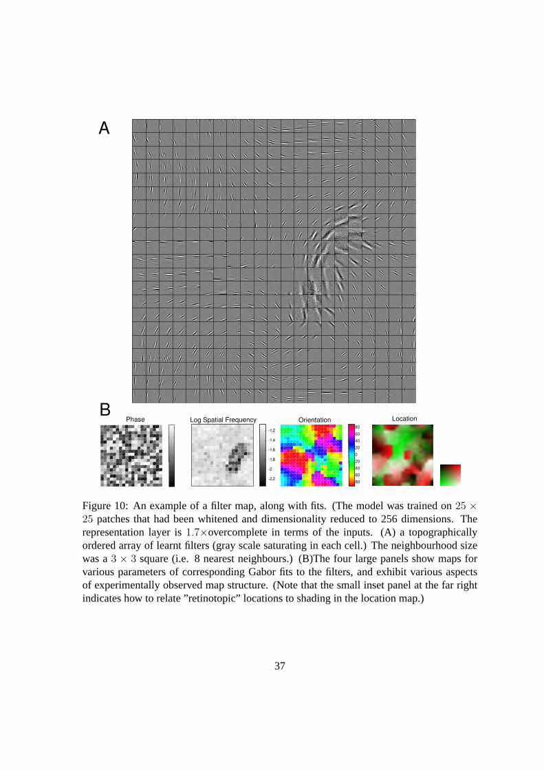
Representative results from such a simulation are given in figure 10. The inputs were

patches of size25 × 25, whitened and dimensionality reduced to vectors of size256; the

representation is1.7× overcomplete. By simple inspection of the filters in panel 10 (A) we

see that there is strong local continuity in the receptive field properties of orientation and

spatial frequency and location, with little continuity of spatial phase. We can make these

feature maps more apparent by plotting the parameters of a Gabor fit to the learnt filters, as

shown in figure 10 (B). Doing this highlights several features that have been experimentally

observed in mapsin vivo — in particular we see singularities in the orientation map and a

low frequency cluster in the spatial frequency map which seems to be somewhat aligned

with one of the pinwheels. Whilst the map of retinotopy shows good local structure, there

is poor global structure. We suggest that this may be due to the relatively small scale of the

model and the use of toroidal boundary conditions (which eliminated the need to deal with

edge effects.)

4.5 PoT’s Applied To Stereo Data

We have also carried out some basic investigations using “synthetic” stereo pairs of natural

scenes. There are few high quality datasets of natural-scene stereo-pairs freely available,

so we generated “synthetic pairs” by creating data sets in which laterally shifted pairs of

patches were extracted from sets of mono-images. Patches were selected with a distribution

of offsets, as illustrated by figure 11, and in doing so we hope to replicate the shifts that

would be caused on this scale due to disparity between the two eyes. Of course, this is

only a crude approximation because we are ignoring the effects that would be caused by

36

Phase

80

60

40

20

0

20

40

60

80

-2.2

-2

-1.8

-1.6

-1.4

-1.2

B

A

LocationLog Spatial Frequency Orientation

Figure 10: An example of a filter map, along with fits. (The model was trained on25 ×25 patches that had been whitened and dimensionality reduced to 256 dimensions. Therepresentation layer is1.7×overcomplete in terms of the inputs. (A) a topographicallyordered array of learnt filters (gray scale saturating in each cell.) The neighbourhood sizewas a3 × 3 square (i.e. 8 nearest neighbours.) (B)The four large panels show maps forvarious parameters of corresponding Gabor fits to the filters, and exhibit various aspectsof experimentally observed map structure. (Note that the small inset panel at the far rightindicates how to relate ”retinotopic” locations to shading in the location map.)

37

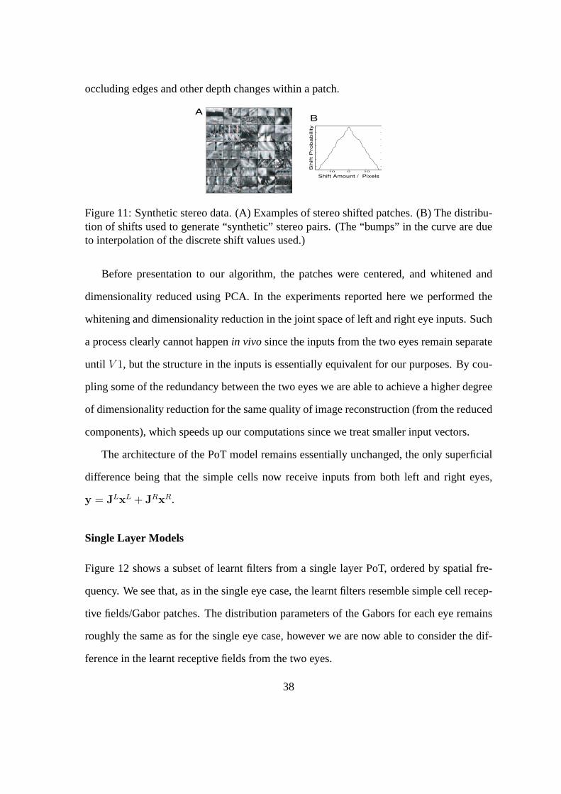
occluding edges and other depth changes within a patch.

-10 0 10

AB

Shift Amount / Pixels

Shift P

robability

Figure 11: Synthetic stereo data. (A) Examples of stereo shifted patches. (B) The distribu-tion of shifts used to generate “synthetic” stereo pairs. (The “bumps” in the curve are dueto interpolation of the discrete shift values used.)

Before presentation to our algorithm, the patches were centered, and whitened and

dimensionality reduced using PCA. In the experiments reported here we performed the

whitening and dimensionality reduction in the joint space of left and right eye inputs. Such

a process clearly cannot happenin vivo since the inputs from the two eyes remain separate

until V 1, but the structure in the inputs is essentially equivalent for our purposes. By cou-

pling some of the redundancy between the two eyes we are able to achieve a higher degree

of dimensionality reduction for the same quality of image reconstruction (from the reduced

components), which speeds up our computations since we treat smaller input vectors.

The architecture of the PoT model remains essentially unchanged, the only superficial

difference being that the simple cells now receive inputs from both left and right eyes,

y = JLxL + JRxR.

Single Layer Models

Figure 12 shows a subset of learnt filters from a single layer PoT, ordered by spatial fre-

quency. We see that, as in the single eye case, the learnt filters resemble simple cell recep-

tive fields/Gabor patches. The distribution parameters of the Gabors for each eye remains

roughly the same as for the single eye case, however we are now able to consider the dif-

ference in the learnt receptive fields from the two eyes.

38

Figure 12: Stereo receptive fields. A random subset of121 stereo-pair filters taken froma 1.7× overcomplete PoT model. Each rectangle demarcated by solid lines represents asingle unit, the left and right halves of the each rectangle (itself split by a dotted line) showthe filter for the left and right eye respectively. The filters have been ordered roughly byspatial frequency.

It is immediately clear that whilst most units have comparable inputs from both eyes

we see some that are strongly dominated by one eye or the other. Of the cells that are

strongly monocular, we note that the majority are of relatively high spatial frequency (as

suggested in Li and Atick (1994)) and that they tend to be closer to45◦ rather than vertical

or horizontal in orientation.

The distribution of ocularity depends on the correlation between the two eyes, in our

case manifested by the distribution of shifts used to generate the synthetic data. For narrow

shift distributions we observed almost entirely binocular (equal strength from both eyes)

units, whilst for independent left and right eye images we saw almost entirely monocular

units. Consequently, we must bear in mind that our results depend on the nature of our

synthetic data set; it would clearly be desirable to use a “real” data set of high quality,

calibrated stereo images (although there are other complications such as vergence and focus

depths).

39

1

9

8

7

6

5

4

3

2

Figure 13: Each row shows the dominant9 filter pairs feeding into a top level “complexcell” unit after training. The solid rectangles depict each unit, with the left and right eyesseparated by a dotted line.

Hierarchical Models

Figure 13 illustrates a collection of “themes” developed by the model if we allow an extra

layer of weights and trainW after initially learning the first layer. We see that as before

there is a clustering based upon orientation, location and spatial frequency. We also note

that some complex cells are predominantly monocular (eg: rows 3 and 4) whilst most are

binocular to various degrees.

We now consider the tuning properties of the units in our models after training. The

(single eye) tuning properties for orientation, phase, spatial frequency and location are

generally the same as those for single eye models, of the type illustrated in figure 9. Ad-

ditionally, we can ask about some properties of stereo tuning — in particular to disparity.

However, answering this question is more difficult than it might initially seem. Analytically

(i.e. based upon the receptive field fits) there is no wholly satisfactory measure; empirically

we are faced with the decision of what to use as a probe stimulus, since this will affect the

results which we obtain (for a discussion of some of these issue see Fleet et al. (1996); Zhu

and Qian (1996); Anzai et al. (1999a,b,c); Hoyer and Hyvarinen (2000).)

40

One possibility is to use the “optimal” stimuli for one eye or the other, but this can lead

to misleading confounds arising from, for instance, the periodicity and orientation within

the stimulus. Another possibility is to use the same sort of images used in training to probe

the disparity tuning. Since our “stereo pairs” are synthetically generated, we have ready

access to naturalistic data in which the offset between left and right eye patterns is known.

By averaging over very many such stimuli, one might hope that this method overcomes

some of the stimulus dependency effects and gives a “truer” measure of tuning.

To generate this naturalistic test data we randomly selected a location in the large im-

age and then extracted a set of patch pairs, at different lateral shifts. Simple cell “tuning

curves” were obtained by taking the filter output to each image at each shift, applying a

half-wave rectification, and then averaging over all such (non-zero) rectified responses at a

given disparity. (The half-wave rectification is necessary to avoid the cancellation effects

that would otherwise be caused by averaging over similar patterns with opposite contrast.)

Complex cell tuning curves were similarly obtained.

Examples of our characterisations of disparity tuning curves are given in figure 14.

We first consider the simple cells. Our examples have been chosen to illustrate the range

of tuning behaviours that we have observed. The top row shows a example of a “tuned

excitatory” type profile, with a symmetric preference for zero disparity. The middle row

illustrates a “tuned inhibitory” type profile, with a symmetric preference for the disparity to

be different from zero. Whilst the bottom row shows an example of asymmetric preference,

“near” or ’far” tuning depending on the direction of asymmetry.

The plots for the complex cells show a similarly interesting range of behaviour. We see

inhibitory and excitatory tuning as in the simple cells and we also see a number of binocular

complex cells with a rather broadinvarianceto disparity. However, in our brief analyses,

we found few complex cells with striking tuning asymmetries.

In addition to these empirical measures, we also consider some simple analytical mea-

41

A B

-10 -5 0 5 10

0

0.2

0.4

0.6

0.8

1

-1

-0.5

0

0.5

1

-10 -5 0 5 10

Left-Right Eye Offset / Pixels Left-Right Eye Offset / Pixels

No

rma

lise

d R

esp

on

se

-10 -5 0 5 10

0

0.2

0.4

0.6

0.8

1

Left-Right Eye Offset / Pixels

No

rma

lise

d R

esp

on

se

Figure 14: (A) Disparity tuning examples for “simple cells”. Each row depicts the resultsfrom a single unit. The central column shows the left- and right-eye receptive field pair forthat unit. The leftmost column shows the average response to5000 image patches at givendisparities. (The output was rectified before taking this average.) The rightmost columnshows the response to the left-eye optimal pattern (dashed curve) and right eye optimalpattern (solid curve). Each curve in this figure has been normalised so that its maximumabsolute value is1.(B) Disparity tuning examples for “complex cells”. Each row depictsthe results from a single top layer unit. The right hand column shows the left- and right-eyereceptive field pairs for the9 simple cells that are most strongly connected to that unit.The left hand column shows the normalised, average response to5000 image patches atdifferent disparities.

42

sures for simple cells based upon the Gabor fits to the left- and right-eye receptive fields

(based upon the analysis of Anzai et al. (1999a)).

We will consider: (i) the phase offset,dφp, between the left and right eye filters; (ii) the

amount of lateral shift spatially, due to phase difference, of the underlying Gabor carriers,

dφv; and also (iii) the lateral shift of the underlying Gabor envelopedX . These quantities

are given by,

dφp = φL − φR (37)

dφv = (φL

2πfL

− φR

2πfR

) cos(θL + θR

2) (38)

dX = xL − xR (39)

Figure 15 shows histograms for these measures from a typical model after training. (We

also looked for correlations between these measures and other parameters such as spatial

frequency and orientation, however no significant trends could be discerned.) The phase

offset, dφp is a measure of the similarity of the two receptive fields and we note a slight

tendency for pairs to be formed that are in phase or anti-phase, with each other. Bothdφv

anddX are spatial measures relating to the lateral shift of the left and right eye receptive

fields. We note that the range of shifts due to location difference is significantly larger than

than for phase shifts, suggesting that in our model position disparity plays a larger role than

phase disparity. This goes somewhat against the current understanding of receptive fieldsin

vivo, although the debate about the relative significance of the two mechanisms is ongoing

(for example Anzai et al. (1999a); Prince et al. (2002)).

Topographic Maps For Stereo Inputs

We have also applied our topographic PoT models to stereo pairs of input patches. The

goal here was to incorporate maps of ocular dominance and disparity alongside those for

43

1 2 30

20

40

60

80

A

-2 0 20

50

100

150

B

-10 0 100

50

100

150

C

Figure 15: Typical histograms of different measures of simple cell disparity from a trainedmodel, based upon Gabor fits to left and right eye receptive fields. (A) Phase offset (moduloπ) dφp. (B) Spatial disparity due to phase differencedφv. (C) Spatial disparity due to Gaborenvelope offsetdX .

orientation, spatial frequency and retinotopy. We present preliminary results in figures 16

and 17, which show a map for ocular dominance (ocularity) in addition to those for phase,

location, orientation and spatial frequency. We consider the ocularity4O of a simple cell

as being the sum of absolute weight values from the left eye, minus the sum of absolute

weight values from the right eye, i.e.

(4O)i =∑

j

(|JLij | − |JR

ij |)

(40)

We see that there is some patterned ocular dominance structure concomitant with the

map properties already outlined. Although this organisation is rather weaker and much

more patchy, there does seem to be a tendency towards interdigitated left and right eye

preferring domains as is foundin vivo. We speculate that such maps may be better defined

in larger models that use genuine stereo inputs, a larger factor of overcompleteness and

appropriate construction of neighbourhood interactions.

44

Figure 16: (A) Map showing right eye filters only. Left eye filters have been set to zerofor this plot. (B) Map showing left eye filters only. Right eye filters have been set to zerofor this plot. (C) Joint map showing topographically ordered filter pairs for both eyes.Not that each unit is plotted independently normalised to fill the full gray scale in eachplot; consequently, monocular regions preferring the ’other eye” appear as noisy patches inpanels B and C.

45

A

B

-0.6 -0.4 -0.2 0 0.2 0.4 0.6

20

40

60

80

100

120

140

C

Phase Orient Log FreqLocation

Ocular Dominance Ocularity

Figure 17: (A) Feature maps for phase, location, orientation and log frequency. (B) Featuremap for ocular dominance. (C) Histogram of ocularity.

5 Relation to Earlier Work

5.1 Gaussian Scale Mixtures

We can consider the complete version of our model as a Gaussian scale mixture (Andrews

and Mallows, 1974; Wainwright and Simoncelli, 2000; Wainwright et al., 2000) with a

particular (complicated) form of scaling function.13

The basic form for a GSM density for a variable,g, can be given as followsWainwright

and Simoncelli (2000),

pGSM(g) =

∫ ∞

−∞

1

(2π)N2 |cQ| 12

exp

(−gT (cQ)−1g

2

)φc(c)dc (41)

wherec is a non-negative scalar variate and andQ is a positive definite covariance matrix.

This is the distribution that results if we drawc from φc(c) and a variablev from a multi-

13In simple terms a GSM density is one that can be written as a (possibly infinite) mixture of Gaussiansthat differ only in the scale of their covariance structure. A wide range of distributions can be expressed inthis manner.

46

dimensional GaussianNV(0,Q) and then takeg =√

cv.

Wainwright et al. (2000) discuss a more sophisticated model in which the distributions

of coefficients in a wavelet decomposition for images are described by a GSM which has

a separate scaling variable,ci, for each coefficient. Theci have a Markov dependency

structure based on the multi-resolution tree which underlies the wavelet decomposition.

In the complete setting, where they variables are in linear one-to-one correspondence

with the input variables,x, we can interpret the distributionp(y) as a Gaussian scale mix-

ture. To see this we first rewritep(y,u) = p(y|u)p(u), wherep(y|u) =∏

j Nyj[0, (

∑i Wijui)

−1]

is Gaussian (see Eqn.13). The distributionp(u) needs to be computed by marginalizing

p(x,u) in Eqn. 11 overx resulting in,

p(u) =1

Zu

∏i

e−uiuiαi−1

∏

k

(∑j

Wjkuj

)− 12

(42)

The partition functionZu ensures normalisation. Thus we see indeed that the marginal

distribution of each of theyi is a Gaussian scale mixture in which the scaling variate for

yi is given byci(u) = (∑

j Wjiuj)−1. The neighbourhoods defined byW in our model

play an analogous role to the tree structure cascade process in Wainwright et al. (2000),

and determine the correlations between the different scaling coefficients.

The overcomplete version of our PoT is not so easily interpreted as a GSM because the

{yi} are no longer independent givenu, nor is the distribution overx a simple GSM due to

the way in whichu is incorporated into the covariance matrix (see equation 8). However,

much of the flavour of a GSM remains.

5.2 Relationship to TICA

In this section we show that, in the complete case, the topographic PoT model is isomorphic

to the model optimised (but not the one initially proposed) by Hyvarinen et al. (2001) in

47

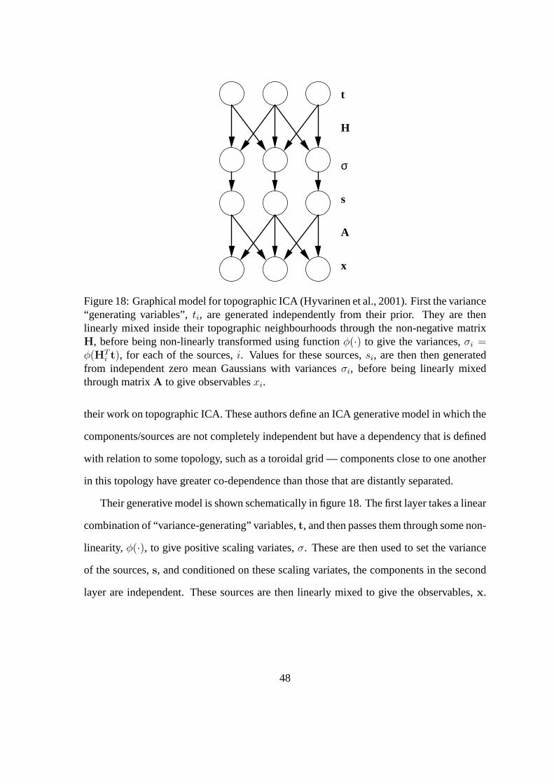
t

x

A

s

σ

H

Figure 18: Graphical model for topographic ICA (Hyvarinen et al., 2001). First the variance“generating variables”,ti, are generated independently from their prior. They are thenlinearly mixed inside their topographic neighbourhoods through the non-negative matrixH, before being non-linearly transformed using functionφ(·) to give the variances,σi =φ(HT

i t), for each of the sources,i. Values for these sources,si, are then then generatedfrom independent zero mean Gaussians with variancesσi, before being linearly mixedthrough matrixA to give observablesxi.

their work on topographic ICA. These authors define an ICA generative model in which the

components/sources are not completely independent but have a dependency that is defined

with relation to some topology, such as a toroidal grid — components close to one another

in this topology have greater co-dependence than those that are distantly separated.

Their generative model is shown schematically in figure 18. The first layer takes a linear

combination of “variance-generating” variables,t, and then passes them through some non-

linearity, φ(·), to give positive scaling variates,σ. These are then used to set the variance

of the sources,s, and conditioned on these scaling variates, the components in the second

layer are independent. These sources are then linearly mixed to give the observables,x.

48

The joint density for(s, t) is given by

p(s, t) =∏

i

psi

(si

φ (HTi t)

)pti(ti)

φ (HTi t)

(43)

and the log-likelihood of the data given the parameters is

L(B) =∑datax

∫ ∏i

psi

(BT

i x

φ (HTi t)

)pti(ti)

φ (HTi t)

| detB|dt (44)

whereB = A−1.

As noted in their paper, the data likelihood is intractable to compute because of the

integral over possible states oft. This prompts the authors to derive an approach that

makes various simplifications and approximations to give a lower bound on the likelihood.

Firstly, they restrict the form of the base density fors to be gaussian14 andφ(·) is taken

to be(·)− 12 . This yields the following expression for the marginal density ofs,

p(s) =

∫1

(2π)d2

exp

(−1

2

∑

k

tk

[∑i

h(i, k)s2i

]) ∏i

pti(ti)√

HTi tdt (45)

This expression is then simplified by the approximation,

√HT

i t ≈√

h(i, i)tk (46)

Whilst this approximation may not always be a good one, it is a strict lower bound on

the true quantity and thus allows for a lower bound on the likelihood as well. Their final

approximate likelihood objective,̃L(B), is then given by,

L̃(B) =∑

data

(d∑

j=1

G

(d∑

i=1

h(i, j)(BTi x)2

)+ log | det(B)|

)(47)

14Their model can therefore be considered as type of GSM, although the authors do not comment on this.

49

where the form of the scalar functionG is given by,

G(τ) = log

∫1√2π

exp

(1

2tτ

)pt(t)

√h(i, i)dt (48)

The results obtained by Hyvarinen and Hoyer (2001); Hyvarinen et al. (2001) are very

similar to those presented here in section 4. These authors also noted the similarity between

elements of their model and the response properties of simple and complex cells in V1.

Interestingly, the optimisation problem that theyactually solve (i.e. maximisation of

equation 47), rather than the one they originally propose, can be mapped directly onto

the optimisation problem for a square, topographic PoT model if we take:B ≡ JPoT,

h(i, j) = WPoTij andG(τ) = log(1 + 1

2τ). More generally, we can construct an equiva-

lent, square energy-based model whose likelihood optimisation corresponds exactly to the

optimisation of their “approximate” objective function. In this sense, we feel that our per-

spective has some advantages. Firstly, in that we have a more accurate picture of what

model we areactually (trying) to optimise. Secondly, in that we are able to move more

easily to overcomplete representations. If Hyvarinen et al. were to make their model over-

complete there would no longer be a deterministic relationship between their sourcess and

x — this additional complication would make the already difficult problems of inference

and learning significantly harder. Thirdly, in the HPoT framework we are able to learn the

top-level weightsW in a principled way using the techniques discussed in section 3.3.

5.3 Representational differences between (TH)PoT & (T)ICA

As well as specifying different probabilistic models, overcomplete energy-based models

such as the PoT differ from overcomplete causal models in the types of representation they

(implicitly) entail. This has interesting consequences when we consider the “population

codes” suggested by the two types of model. We focus on the representation in the first layer

50

(“simple cells”), although similar arguments might be made as we proceed hierarchically.

In an overcomplete causal model, many configurations of the sources are compatible

with a configuration of the input.15 For a given input, a posterior distribution is induced

over the sources in which the inferred values for different sources are conditionally depen-

dent. As a result, although linear in the generative direction, the formation of a posterior

representation in overcomplete causal models is essentiallynon-linearand moreover it is

non-localdue to the lack of conditional independence. This implies that unlike EBM’s

inference in causal models is often iterative if not intractable and therefore certainly time

consuming. Also, although we can specify the basis functions associated with a unit, it is

much harder to specify any kind of feed-forward receptive field in causal models. The issue

of how such a posterior distribution could be encoded in a representation remains open; a

common postulate (made on the grounds of efficient coding) is that a maximum a posteriori

(MAP) representation should be used, but we note that even computing the MAP value is

usually iterative and slow.

Conversely, in overcomplete EBM’s with deterministic hidden units such as we have

presented in this paper, the mapping from inputs to representations remains simple and

non-iterative and requires only local information.

In figure 19 we try to schematically illustrate a salient consequence of this difference

between EBM’s and causal models. Panel (A) shows an array of image vectors which

should be understood to be either a subset of the basis functions in an overcomplete causal

model, or a subset of the filters in overcomplete PoT model. In panel (B) we illustrate

the way in which four example inputs are represented; these inputs have been chosen to

be four of the vectors shown in panel (A). The left-hand column of panel (C) shows the

responses of the units in an EBM-style model, whilst the right-hand column shows the

15In fact, strictly speaking there is a subspace of of source configurations of the same dimensionality as theinput space.

51

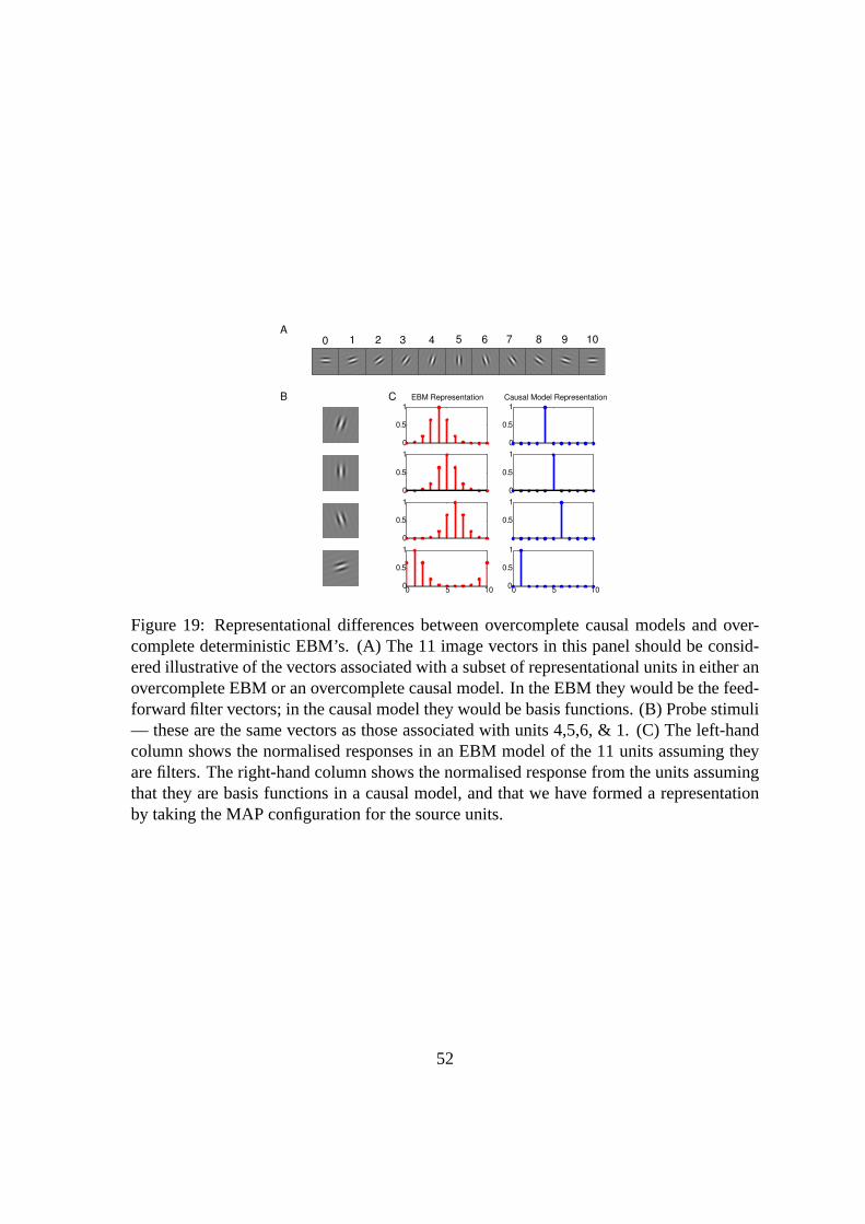
0

0.5

1

0

0.5

1

0

0.5

1

0

0.5

1

0

0.5

1

0.5

1

0 5 100

0.5

1

0 5 100

0.5

1

A

B

0 321 4 765 1098

EBM Representation Causal Model RepresentationC

Figure 19: Representational differences between overcomplete causal models and over-complete deterministic EBM’s. (A) The 11 image vectors in this panel should be consid-ered illustrative of the vectors associated with a subset of representational units in either anovercomplete EBM or an overcomplete causal model. In the EBM they would be the feed-forward filter vectors; in the causal model they would be basis functions. (B) Probe stimuli— these are the same vectors as those associated with units 4,5,6, & 1. (C) The left-handcolumn shows the normalised responses in an EBM model of the 11 units assuming theyare filters. The right-hand column shows the normalised response from the units assumingthat they are basis functions in a causal model, and that we have formed a representationby taking the MAP configuration for the source units.

52

MAP responses from an overcomplete causal model.

This is admittedly an extreme case, but it provides an good illustration of the point

we wish to make. More generally, although representations in an overcomplete PoT are

sparse there is also some redundancy; the PoT population response is typically less sparse

(Willmore and Tolhurst, 2001) than an “equivalent” causal model.

Interpreting the two models as a description of neural coding, one might expect the

EBM representation to be more robust to the influences of neural noise as compared with

the representation suggested from a causal approach. Furthermore, the EBM style repre-

sentation is shiftable — it has the property that for small changes in the input there are

small changes in the representation. This property would not necessarily hold for a highly

overcomplete causal model. Such discontinuous representation might make subsequent

computations difficult and non-robust, and it also seems somewhat at odds with the neuro-

biological data — however proper comparison is difficult since there is no real account of

dynamic stimuli or spiking in either model. At present, it remains unclear which type of

model — causal or energy-based — provides the more appropriate description of coding in

the visual system, especially since there are many aspects that neither approach captures.

5.4 Divisive Normalisation

Wainwright et al. (2000) also show that Gaussian scale mixtures, with appropriate choices

of the distribution of scaling variables, are able to capture a particular form of higher order

structure found in images. This structure is evident in the correlations between (square)

rectified outputs of linear filters applied to natural scene ensembles. Even when the raw

filter outputs themselves are uncorrelated, there is often dependency between their rectified

outputs. This can be demonstrated neatly by so-called bow-tie plots in which the distribu-

tion for the output of one filterconditionedon the output of another filter is plotted. An

53

A B

C D

Figure 20: (A) Joint histogram of responses for two neighbouring filters from a topographicmodel. (B) Conditional histogram for response of one filter given the response of the sec-ond. Note the characteristic “bow tie” shape — whilst the linear responses are uncorrelated,there is a magnitude of the two filter responses. Filter 2 is much more likely to respondstrongly when filter 1 is also responding strongly. (C) Divisively normalised joint responsehistogram using Eqn.50. (D) Conditional histogram of divisively normalised responses.Clearly, in going from (B) to (D) most of the higher order dependencies have been re-moved by divisive normalisation (this effect is much harder to discern in joint histogramsthan in conditional histograms).

example of such bow-tie plots for the filters learnt using a square implementation of our

PoT is given in figure 20 (B).

This “bow-tie” phenomenon has also been given prominence in the context of under-

standing “divisive normalisation” of V1 responses (Simoncelli and Schwartz, 1999; Wain-

wright et al., 2001; Cavanaugh et al., 2002a,b). In these approaches the authors suggest a

divisive normalisation of the form given in equation 49 might help to remove higher order

dependency from the simple cell responses.

R∗j =

L2j

σ2j +

∑j ωjkL2

k

(49)

whereσ2j andωjk are free parameters andLk are the outputs of linear filters applied to an

54

image. Their parameters are chosen to minimise the expectation of(log(R∗

j

))2 over a set

of input patterns. This can also be somewhat related to the GSM framework.

We note that the divisive interaction in equation 49 is extremely similar to the form that

would arise in our framework if we inferred the MAP estimate ofu, given an input pattern,

and then used these{ui} to recover “underlying” Gaussian variates. So, it is natural to

investigate how the learnt weightsW perform at removing this higher order redundancy.

We derive divisive normalisation (or “gaussianisation”) in our model as,

y∗i = yi

(∑j

Wji(αj − 1)

1 + 12zj

) 12

(50)

wherey are the first layer deterministic hidden units andz are the units of the second layer.

Figure 20 (D) shows an example of the results of such an operation. We see that there

is much greater independence between the normalised responses and the raw responses.

Furthermore, we note that the information required to perform the normalisation is present

within the activities of the top layer activities,z — our “complex cells”.

Combining this with earlier results, it is tempting to postulate the existence of cortical

micro-circuitry in which complex cell responses feed back (via interneurons) to divisively

normalise simple cell responses — although this is complicated by the fact that complex

cells themselves also experience divisive normalisation effects.

6 Summary

We have presented a hierarchical energy-based density model that we suggest is generally

applicable to data-sets that have a sparse structure, or that can be well characterised by

constraints that are often well-satisfied, but occasionally violated by a large amount.

By applying our model to natural scene images we are able to provide an interpreta-

55

tional account for many aspects of receptive field and topographic map structure within pri-

mary visual cortex, and which also develops sensible high-dimensional population codes.

Deterministic features (i.e. the first- and second-layer filter outputs) within our model play

a key role in defining the density of a given image patch, and we are able to make a close

relationship between these features and the responses of simple cells and complex cells in

V1. Furthermore, by constraining our model to interact locally we are able to provide some

computational motivation for the forms of the cortical maps for retinotopy, phase, spatial

frequency and orientation. Preliminary results also suggest that stereo response properties

and the maps for ocular dominance might be similarly explained.

Whilst our model is closely related to some previous work, most prominently Hyvarinen

et al. (2001), it is importantly different in its formulation and describes different statistical

relations in the overcomplete case, and bestows a different interpretation on the learnt fea-

tures. We are not aware of any other high-dimensional, statistically-motivated models that

have been used to give accounts for this range of topographic maps — particularly stereo

tuning and ocular dominance as well as orientation, spatial frequency, position and phase

— along with accounts for simple and complex cell responses in an overcomplete setting.

We present our model as both a general alternative tool to ICA for describing sparse data

distributions, and also as an alternative interpretive account for some of the neurobiological

observations from the mammalian visual system.

Acknowledgements

We thank Peter Dayan and Yee Whye Teh for important intellectual contributions to this

work and many other researchers for helpful discussions. The work was funded by the

Gatsby Charitable Foundation, the Wellcome Trust, NSERC, CFI. GEH holds a Canada

Research Chair.

56

Appendices

A Sampling in HPoT models

Complete Models

We start our discussion with sampling in complete HPoT models. In this case there is a

simple invertible relationship betweenx andy, implying that we may focus on sampling

y and subsequently transforming these samples back tox-space throughx = J−1y. Un-

fortunately, unlessW is diagonal, ally variables are coupled throughW, which makes it

difficult to devise an exact sampling procedure. Hence, we resort to Gibbs sampling using

Eqn.12 where we replaceyj = Jjx to acquire sampleu|y. To obtain a sampley|u we

convert Eqn.8 into

P (y|u) = Ny

[y; 0,Diag[WTu]−1

](51)

We iterate this process (alternatingly samplingu ∼ P (u|y) andy ∼ P (y|u)) until the

Gibbs sampler has converged. Note that bothP (u|y) andP (y|u) are factorized distribu-

tions implying that bothu andy variables can be sampled in parallel.

Undercomplete Models

While for the complete case we may simply transform oury-samples tox space through

x = J−1y, the situation is slightly more complex in the undercomplete case. Here, we start

again by running our Gibbs sampler defined above to get a sample fory, but in addition we

also acquire a sample fromy⊥ ∼ Ny⊥ [y⊥; 0, σ2I]. Samples fory andy⊥ are subsequently

combined into a sample inx-space using,

x = PJx + P⊥J x = J#y + KTy⊥ (52)

57

wherePJ is the projection operator onto the space space spanned by the rows ofJ, while

P⊥J is the projection operator onto its complement subspace given by Eqn.19. Moreover,

J# = JT (JJT )−1 is the pseudo-inverse ofJ.

To explicitly compute an orthonormal basisKT we can compute the following SVD

decompositionABCT = SV D([JT |0]). The lastD − M columns ofA then form and

orthonormal basis in the complement subspace,A = [ADM |KT ]. Moreover, the pseudo-

inverse ofJ can also be computed asJ# = ADMB−1MMCT

MM . Alternatively, we can sam-

ple x′ ∼ Nx[x′|0, σ2I] and subsequently project the samples on the orthogonal subspace:

KTy⊥ = P⊥x′.

Overcomplete Models

In the overcomplete case we are no longer allowed to first sample they variables, and sub-

sequently transform them intox space. The reason is that the deterministic relationy = Jx

means that when there are morey variables thanx variables, somey configurations are not

allowed, i.e. they are not in the range of the mappingx → Jx with x ∈ R. If we sample

y, all these samples (with probability one) will have some components in these forbidden

dimensions, and it is unclear how to transform them correctly intox-space. An approxima-

tion is obtained by projecting they-samples intox-space using̃x = J#y. We have often

used this approximation in our experiments and have obtained good results, but we note

that its accuracy is expected to decrease as we increase the degree of overcompleteness.

A more expensive but correct sampling procedure for the overcomplete case is to use

a Gibbs chain in the variablesu and x (instead ofu and y) by using Eqns.12 and 13

directly. In order to samplex|u we need to compute a Cholesky factorization of the inverse-

covariance matrix of the Gaussian distributionP (x|u),

RTR = JVJT V = Diag[WTu] (53)

58

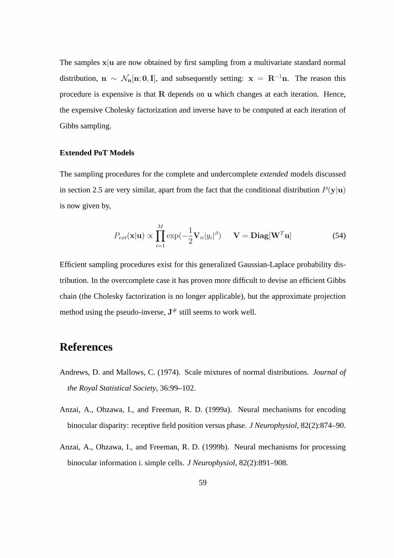
The samplesx|u are now obtained by first sampling from a multivariate standard normal

distribution, n ∼ Nn[n;0, I], and subsequently setting:x = R−1n. The reason this

procedure is expensive is thatR depends onu which changes at each iteration. Hence,

the expensive Cholesky factorization and inverse have to be computed at each iteration of

Gibbs sampling.

Extended PoT Models

The sampling procedures for the complete and undercompleteextendedmodels discussed

in section 2.5 are very similar, apart from the fact that the conditional distributionP (y|u)

is now given by,

Pext(x|u) ∝M∏i=1

exp(−1

2Vii|yi|β) V = Diag[WTu] (54)

Efficient sampling procedures exist for this generalized Gaussian-Laplace probability dis-

tribution. In the overcomplete case it has proven more difficult to devise an efficient Gibbs

chain (the Cholesky factorization is no longer applicable), but the approximate projection

method using the pseudo-inverse,J# still seems to work well.

References

Andrews, D. and Mallows, C. (1974). Scale mixtures of normal distributions.Journal of

the Royal Statistical Society, 36:99–102.

Anzai, A., Ohzawa, I., and Freeman, R. D. (1999a). Neural mechanisms for encoding

binocular disparity: receptive field position versus phase.J Neurophysiol, 82(2):874–90.

Anzai, A., Ohzawa, I., and Freeman, R. D. (1999b). Neural mechanisms for processing

binocular information i. simple cells.J Neurophysiol, 82(2):891–908.

59

Anzai, A., Ohzawa, I., and Freeman, R. D. (1999c). Neural mechanisms for processing

binocular information ii. complex cells.J Neurophysiol, 82(2):909–24.

Atick, J. J. and Redlich, A. N. (1992). What does the retina know about natural scenes.

Neural Computation, 4(2):196–210.

Bartholomew, D. (1987).Latent Variable Models and Factor Analysis. Charles Griffin &

Co Ltd.

Bell, A. J. and Sejnowski, T. J. (1995). An information maximization approach to blind

separation and blind deconvolution.Neural Computation, 7(6):1129–1159.

Bell, A. J. and Sejnowski, T. J. (1997). The ”independent components” of natural scenes

are edge filters.Vision Research, 37(23):3327–3338.

Carreira-Perpinan, M. and Hinton, G. (2005). On contrastive divergence learning. InArti-

ficial Intelligence and Statistics.

Cavanaugh, J. R., Bair, W., and Movshon, J. A. (2002a). Nature and interaction of signals

from the receptive field center and surround in macaque v1 neurons.J Neurophysiol,

88(5):2530–46.

Cavanaugh, J. R., Bair, W., and Movshon, J. A. (2002b). Selectivity and spatial distribution

of signals from the receptive field surround in macaque v1 neurons.J Neurophysiol,

88(5):2547–56.

Deerwester, S., Dumais, S., Landauer, T., Furnas, G., and Harshman, R. (1990). Indexing

by latent semantic analysis.Journal of the American Society of Information Science,

41(6):391–407.

Fleet, D. J., Wagner, H., and Heeger, D. J. (1996). Neural encoding of binocular disparity:

energy models, position shifts and phase shifts.Vision Res, 36(12):1839–57.

60

Freund, Y. and Haussler, D. (1992). Unsupervised learning of distributions of binary vec-

tors using 2-layer networks. InAdvances in Neural Information Processing Systems,

volume 4, pages 912–919.

Heskes, T. (1998). Selecting weighting factors in logarithmic opinion pools. In Jordan,

M. I., Kearns, M. J., and Solla, S. A., editors,Advances in Neural Information Processing

Systems, volume 10. The MIT Press.

Hinton, G. and Teh, Y. (2001). Discovering multiple constraints that are frequently ap-

proximately satisfied. InProceedings of the Conference on Uncertainty in Artificial

Intelligence, pages 227–234, Seattle, Washington.

Hinton, G. E. (2002). Training products of experts by minimizing contrastive divergence.

Neural Computation, 14(8):1771–1800.

Hoyer, P. O. and Hyvarinen, A. (2000). Independent component analysis applied to feature

extraction from colour and stereo images.Network-Computation in Neural Systems,

11(3):191–210.

Hyvarinen, A. and Hoyer, P. O. (2001). A two-layer sparse coding model learns simple

and complex cell receptive fields and topography from natural images.Vision Research,

41(18):2413–2423.

Hyvarinen, A., Hoyer, P. O., and Inki, M. (2001). Topographic independent component

analysis.Neural Computation, 13(7):1527–1558.

Lewicki, M. and Sejnowski, T. (2000). Learning overcomplete representations.Neural

Computation, 12:p.337–365.

Li, Z. and Atick, J. J. (1994). Efficient stereo coding in the multiscale representation.

Network-Computation in Neural Systems, 5:157–174.

61

Marks, T. K. and Movellan, J. R. (2001). Diffusion networks, products of experts, and

factor analysis. Technical Report UCSD MPLab TR 2001.02, University of California

San Diego.

Olshausen, B. A. and Field, D. J. (1996). Emergence of simple-cell receptive field proper-

ties by learning a sparse code for natural images.Nature, 381:607–610.

Olshausen, B. A. and Field, D. J. (1997). Sparse coding with an overcomplete basis set: A

strategy employed by v1?Vision Research, 37(23):3311–3325.

Portilla, J., Strela, V., Wainwright, M., and Simoncelli, E. P. (2003). Image denoising

using scale mixtures of gaussians in the wavelet domain.IEEE Trans Image Processing,

12(11):1338–1351.

Prince, S. J., Cumming, B. G., and Parker, A. J. (2002). Range and mechanism of encoding

of horizontal disparity in macaque v1.J Neurophysiol, 87(1):209–21.

Ringach, D. L. (2002). Spatial structure and symmetry of simple-cell receptive fields in

macaque primary visual cortex.J Neurophysiol, 88(1):455–63.

Simoncelli, E. (1997). Statistical models for images: Compression, restoration and syn-

thesis. In31st Asilomar Conference on Signals, Systems and Computers, Pacific Grove,

CA.

Simoncelli, E. P. and Schwartz, O. (1999). Modeling surround suppression in v1 neurons

with a statistically-derived normalization model. InAdvances in Neural Information

Processing Systems 11, volume 11, pages 153–159.

Smolensky, P. (1986). Information processing in dynamical systems: foundations of har-

mony theory. In Rumehart, D. and McClelland, J., editors,Parallel Distributed Process-

62

ing: Explorations in the Microstructure of Cognition. Volume 1: Foundations. McGraw-

Hill, New York.

Teh, Y., Welling, M., Osindero, S., and Hinton, G. (2003). Energy-based models for sparse

overcomplete representations.Journal of Machine Learning Research - Special Issue on

ICA, 4:1235–1260.

Tipping, M. and Bishop, C. (1999). Probabilistic principal component analysis.Journal of

the Royal Statistical Society, Series B, 21(3):611–622.

van Hateren, J. H. and van der Schaaf, A. (1998). Independent component filters of natural

images compared with simple cells in primary visual cortex.Proc R Soc Lond B Biol

Sci, 265(1394):359–66.

Wainwright, M. J., Schwartz, O., and Simoncelli, E. P. (2001). Natural image statistics and

divisive normalisation: Modeling nonlinearities and adaptation in cortical neurons. In

Rao, R. P. N., Olshausen, B. A., and Lewicki, M. S., editors,Statistical Theories Of The

Brain. MIT Press.

Wainwright, M. J. and Simoncelli, E. P. (2000). Scale mixtures of gaussians and the statis-

tics of natural images. InAdvances in Neural Information Processing Systems 12, vol-

ume 12, pages 855–861.

Wainwright, M. J., Simoncelli, E. P., and Willsky, A. S. (2000). Random cascades of

gaussian scale mixtures and their use in modeling natural images with application to de-

noising. In7th International Conference on Image Processing, Vancouver, BC, Canada.

IEEE Computer Society.

Welling, M., Agakov, F., and Williams, C. (2003a). Extreme components analysis. In

Advances in Neural Information Processing Systems, volume 16, Vancouver, Canada.

63

Welling, M., Hinton, G., and Osindero, S. (2002a). Learning sparse topographic repre-

sentations with products of student-t distributions. InAdvances in Neural Information

Processing Systems, volume 15, Vancouver, Canada.

Welling, M., Zemel, R., and Hinton, G. (2002b). Self-supervised boosting. InAdvances in

Neural Information Processing Systems, volume 15, Vancouver, Canada.

Welling, M., Zemel, R., and Hinton, G. (2003b). A tractable probabilistic model for projec-

tion pursuit. InProceedings of the Conference on Uncertainty in Artificial Intelligence.

Welling, M., Zemel, R., and Hinton, G. (2004). Probabilistic sequential independent com-

ponents analysis.IEEE-Transactions in Neural Networks , Special Issue on Information

Theory.

Williams, C., Agakov, F., and Felderhof, S. (2001). Products of gaussians. InAdvances in

Neural Information Processing Systems, volume 14, Vancouver, CA.

Williams, C. K. I. and Agakov, F. (2002). An analysis of contrastive divergence learn-

ing in gaussian boltzmann machines. Technical Report EDI-INF-RR-0120, School of

Informatives.

Willmore, B. and Tolhurst, D. J. (2001). Characterizing the sparseness of neural codes.

Network-Computation in Neural Systems, 12(3):255–270.

Yuille, A. (2004). A comment on contrastive divergence. Technical report, Department

Statistics and Psychology UCLA. Technical Report.

Zhu, Y. D. and Qian, N. (1996). Binocular receptive field models, disparity tuning, and

characteristic disparity.Neural Comput, 8(8):1611–41.

64