Modelling the performance of underground heat exchangers and storage systems Master of Science Thesis in the Master’s Programme Structural Engineering and Building Performance Design DAVID VAN REENEN Department of Civil and Environmental Engineering Division of Building Technology Building Physics CHALMERS UNIVERSITY OF TECHNOLOGY Göteborg, Sweden 2011 Master’s Thesis 2011:83

Welcome message from author
This document is posted to help you gain knowledge. Please leave a comment to let me know what you think about it! Share it to your friends and learn new things together.
Transcript
Modelling the performance of
underground heat exchangers and
storage systems
Master of Science Thesis in the Master’s Programme Structural Engineering and
Building Performance Design
DAVID VAN REENEN
Department of Civil and Environmental Engineering
Division of Building Technology
Building Physics
CHALMERS UNIVERSITY OF TECHNOLOGY
Göteborg, Sweden 2011
Master’s Thesis 2011:83


MASTER’S THESIS 2011:83
Modelling the performance of
underground heat exchangers and
storage systems
Master of Science Thesis in the Master’s Programme Structural Engineering and
Building Performance Design
DAVID VAN REENEN
Department of Civil and Environmental Engineering
Division of Building Technology
Building Physics
CHALMERS UNIVERSITY OF TECHNOLOGY
Göteborg, Sweden 2011

Modelling the Performance of Underground Heat Exchangers and Storage Systems
Master of Science Thesis in the Master’s Programme Structural Engineering and
Building Performance Design
DAVID VAN REENEN
© DAVID VAN REENEN, 2011
Examensarbete / Institutionen för bygg- och miljöteknik,
Chalmers tekniska högskola 2011:83
Department of Civil and Environmental Engineering
Division of Building Technology
Building Physics
Chalmers University of Technology
SE-412 96 Göteborg
Sweden
Telephone: + 46 (0)31-772 1000
Cover:
The illustration on the cover shows a diagram showing the S-function of a ground
heat exchanger, the mesh around a borehole, and the resulting temperature
distribution.
Chalmers Reproservice / Department of Civil and Environmental Engineering
Göteborg, Sweden 2011

I
Modelling the Performance of Underground Heat Exchangers and Storage Systems
Master of Science Thesis in the Master’s Programme Structural Engineering and
Building Performance Design
DAVID VAN REENEN
Department of Civil and Environmental Engineering
Division of Building Technology
Building Physics
Chalmers University of Technology
ABSTRACT
Geothermal heat pumps are systems that combine a closed loop underground heat
exchanger or open loop groundwater heat exchanger along with a heat pump. These
systems use the ground (or ground water) as a source of heat in the winter or cooling
in the winter. When heating and cooling are used on a seasonal basis, the storage of
thermal energy can be accomplished. This is useful to reduce the energy demand of
buildings. The purpose of this thesis project was to investigate and quantify the
performance of ground source heat pumps and underground storage systems. This
study focused on the development of a model of underground heat exchangers and
their integration into complete building systems. The behaviour of ground source heat
pumps and underground storage was numerically evaluated using a combination of
the commercial finite element software COMSOL Multiphysics and Matlab/Simulink.
Various models of underground heat exchangers have been developed that consider
transient conditions of full three dimensional heat transfer interaction between the
ground, the underground pipe network, and the external environment. The model
simplifies the flow in the pipe network to one dimension flow with transverse heat
transfer coupled with a full three dimensional model of the ground to analyze the heat
transfer in the entire system. The underground heat exchanger has been integrated
into a building model. These models are used to simulate the dynamic behaviour of a
building, including all relevant thermal parameters such as heating, cooling, and
control systems. Using S-functions in Simulink, the geothermal heat pump has been
integrated into the building to observe its overall performance. A number of
underground heat exchanger configurations have been studied and their effect on the
overall thermal performance of buildings has been analyzed. The cycling of
temperatures in the ground during heating and cooling seasons has been observed.
The increased cycling of indoor temperature inside a building has also been observed.
This cycling is partially due to the slower response of the heat pump and the fact that
the heat pump turns off and on due to temperature limits.
Key words: Simulation, geothermal heat pumps, underground heat storage, thermal,
whole building simulation

II

CHALMERS Civil and Environmental Engineering, Master’s Thesis 2011:83 III
Contents
ABSTRACT I
CONTENTS III
PREFACE V
NOTATIONS VI
1 INTRODUCTION 1
1.1 Background 1
1.2 Objective and scope 2
1.3 Limitations 2
2 THEORETICAL BACKGROUND 3
2.1 Underground heat exchanger 3
2.2 Heat transfer 4
2.2.1 Heat transfer by conduction 4
2.2.2 A pipe with transverse heat flow 5
2.3 Modelling of conduction and convection 6
3 DEVELOPMENT OF AN UNDERGROUND HEAT EXCHANGER MODEL 8
3.1 Heat conduction 8
3.1.1 Line model with constant heat flux from a horizontal pipe 8
3.1.2 Step Response for a cylinder 12
3.2 Heat convection in a pipe 13
3.2.1 Pipe flow modelled with a one dimensional PDE 13
3.2.2 Pipe flow modelled using a predefined heat transfer module 15
3.2.3 Coupled fluid dynamics and heat transfer 16
3.2.4 Transient simulation of one dimensional fluid flow 19
3.3 Two dimensional conduction coupled to one dimensional convection 23
3.4 Three dimensional conduction coupled to one dimensional convection 24
3.4.1 Fluid flow with a constant ground temperature 24
3.4.2 Fluid flow with a coupled ground temperature 26
3.4.3 Fluid flow in a pipe near ground surface 28
3.4.4 Transient performance of the model 32
4 MODELS OF UNDERGROUND HEAT EXCHANGERS 33
4.1 The COMSOL models 33
4.1.1 Single linear horizontal pipe 33
4.1.2 Single loop BHE 35
4.1.3 Models of multiple single loop BHEs 36
4.2 Simulink and S–Functions 38
4.2.1 A simple embedded model using a S–function 38

CHALMERS, Civil and Environmental Engineering, Master’s Thesis 2011:83 IV
4.3 S–Functions of underground heat exchangers 40
4.3.1 Single linear horizontal pipe 40
4.3.2 Models of BHEs 43
4.4 Step response of BHEs 46
4.5 Heating and cooling step response of BHEs 49
5 INTEGRATION OF UNDERGROUND HEAT EXCHANGERS IN BUILDING
MODELS 51
5.1 Integration into a building system 51
5.1.1 Model of the heat exchangers 52
5.1.2 Modelling of a heat pump 55
5.1.3 Control of the heat pump 57
6 PERFORMANCE OF UNDERGROUND HEAT EXCHANGERS 58
6.1 Response of a simple building model 58
6.1.1 The ISE model of a building 58
6.1.2 Simulation details 61
6.1.3 De Bilt results 66
6.1.4 Gothenburg results 68
6.1.5 Discussion 70
7 CASE STUDY OF AN EXISTING BUILDING: ANATOMY HOUSE 71
7.1 Development of a lumped thermal model 71
7.2 Anatomy House (Anatomi Hus) at Salgrenska Hospital in Gothenburg 73
7.2.1 Building characteristics 74
7.2.2 Simulink model of the building 78
7.2.3 Preliminary simulations of the Anatomy House 82
7.2.4 Development of a model including ground coupled heat pumps 84
7.2.5 Simulation of the Anatomy House with BHEs 86
8 CONCLUSIONS 89
9 RECOMMENDATIONS FOR FURTHER STUDY 90
10 REFERENCES 91
APPENDIX A DETAILS OF THE MODEL COUPLING IN COMSOL 92
APPENDIX B CODE FOR EXAMPLE S–FUNCTIONS 94
APPENDIX C S–FUNCTION OF UNDERGROUND HEAT EXCHANGERS 96

CHALMERS Civil and Environmental Engineering, Master’s Thesis 2011:83 V
Preface
In this thesis project the development of models simulating the performance of
geothermal heat pumps and their integration in buildings has been completed. This
project was carried out from September 2010 to June 2011 as a joint project between
Chalmers University of Technology, Sweden and Technical University of Eindhoven,
Netherlands. The project was jointly supervised by Professor Angela Sasic
Kalagasidis of the Division of Building Technology in the Department of Civil and
Environmental Engineering at Chalmers University of Technology and Assistant
Professor A.W.M. (Jos) van Schijndel of the Division of Building Physics and
Services of the Department of Architecture, Building, and Planning of the Technical
University of Eindhoven.
The project was initiated at Chalmers University of Technology in September 2010
through December 2010. It was continued at the Technical University of Eindhoven
in January 2011 through April 2011. The project was finalized again at Chalmers
University of Technology in May and June 2011.
I would like to thank both Angela Sasic Kalagasidis and Jos van Schijndel for their
help and guidance in the development and conclusion of this project. They have both
been very helpful and supportive. I would also like to thank my colleague, Natalie
Williams Portal, for her support and helpfulness as we worked on separate projects
with the same supervisors.
Gothenburg June 2011
David van Reenen

CHALMERS, Civil and Environmental Engineering, Master’s Thesis 2011:83 VI
Notations
Roman upper case letters
Bi Biot number, [–] ��� Coefficient of performance, [–] � Depth of a pipe in the ground, [m] �� Hydraulic radius, [m] � Fourier number, [–] Length or thickness, [m] �� Mass flow rate, [kg/s] � Nusselt number, [–]
P Pressure, [Pa]
Pr Prandtl number, [–]
Q Heat flow rate, [W] �� Reynolds number, [–]
T Temperature, [K]
Roman lower case letters
�� Specific heat capacity, [J/(kg·K)] � Enthalpy, [J/kg] � Heat pump efficiency, [–] �� Characteristic length, [m] η� Heat exchanger efficiency, [m] � Heat flux, [W/m2] � Fluid velocity, [m/s] � Fluid velocity vector, [m/s] � Time, [s] � Absolute viscosity of water, [m
2/s] �, �, Cartesian coordinates [m]
Greek lower case letters
!" Heat transfer coefficient [W/K·m2] # Thermal conductivity [W/mK] $ Density [kg/m
3] � Heat flow [W/m
2]
Subscripts
� Convective %�� Exterior & Ground ' Interior '( Inlet � Liquid Outer

CHALMERS, Civil and Environmental Engineering, Master’s Thesis 2011:83 1
1 Introduction
1.1 Background
Warming of the global climate is now considered unequivocal as evidenced by
warming temperature in the air and the oceans, melting of snow and ice, and the rising
sea levels (IPCC, 2007). One way to combat global warming is to reduce the energy
demand used for the heating and cooling of buildings.
Geothermal heat pumps are systems that combine a closed loop ground heat
exchanger or open loop groundwater heat exchanger along with a heat pump. These
systems use the ground (or ground water) as a source of heat in the winter and/or
cooling in the summer. In heating mode the ground is used as a condenser while in
the summer the ground is used as an evaporator. A typical installation consists of a
borehole containing two small diameter tubes linked at the bottom with a U–bend.
This is termed a borehole heat exchanger (BHE). For each kWh of heating or cooling
energy that the systems output, an input of 0.22 to 0.35 kWh of electricity is required.
This results in a 30 to 50% lower power consumption than typical air–to–air heat
pump system (Sanner et al., 2003).
Energy storage systems are also used to achieve a reduction in total energy use of
buildings. Excess energy can be captured when available and stored for use when
there is a lower supply or higher demand. This can result in a reduction in the total
and peak energy use of buildings. In buildings, heat is normally the type of energy
that is captured and stored. These storage systems are used to store heat captured
during warm periods and then used to heat the building during colder periods. This
can be done on a diurnal or seasonal basis. It can also be used for storing energy that
can only be generated during limited periods. An example of this is storing solar
energy. Heat storage can be valuable on both a short term and long term basis. In the
short term, energy can be stored for use in diurnal temperature variation or during an
emergency loss of energy supply. Long term storage can allow for seasonal storage of
energy such as described above. Underground thermal energy storage systems can
consist of either open aquifer storage or underground heat storage systems. These
systems can be used for cooling of a building, but also for the storage of solar or other
waste heat that can then be used for seasonal heating (Sanner et al., 2003).
Ground heat storage, using geothermal heat pumps, is an example of long term
storage. It is not as useful for short term storage, but can be successfully used for the
seasonal storage of energy (Hellström, 1991).
Duffie and Beckman (1975) described three requirements for heat storage:
1. It must be able to receive and discharge heat with relatively small
temperature differences.
2. It should have small energy losses
3. It should be inexpensive.
Previous studies have been conducted on geothermal heat pumps and underground
storage systems. They have generally consisted of simplified one dimensional or two
dimensional systems and many have been limited to the long term response of the
systems. This study will focus on the development of a three dimensional model of
the ground and underground heat exchangers. It will include complex modelling of
underground heat exchangers, such as BHEs, and their integration into buildings. It

CHALMERS, Civil and Environmental Engineering, Master’s Thesis 2011:83 2
will also examine the performance of BHEs on their own and as part of a complete
building system.
1.2 Objective and scope
The aim of the project was to investigate underground heat exchangers and model
their short and long term performance. This study focused on the development of a
model for the integration of geothermal heat pumps into buildings and examined their
use as heat storage systems. Numerical analysis was executed using a combination of
Matlab/Simulink and the commercial finite element software COMSOL.
This study is related to previous research conducted on the principles of heat
extraction from the ground by horizontally and vertically buried pipes. A three
dimensional model of underground heat exchangers was developed in COMSOL that
considered both steady state and transient conditions. This model included a full three
dimensional representation of the ground and the borehole. Building models in
Matlab/Simulink have also been studied. The two models were combined to observe
the overall performance of a model building with an integrated geothermal heat pump
system. A parametric study of a simplified building model along with a case study of
an existing building is presented to accomplish this.
This thesis report documents details of the development of a model for underground
heat exchanger along with some theoretical background of the model. It details the
integration of this model into a building model and the performance of the system as
part of a typical building and a case study of an existing building.
1.3 Limitations
This study has focused on the development of a model for ground–coupled heat
pumps. It has focused on two types of systems: a horizontal pipe parallel and near the
ground surface and BHEs. Other types of systems were not considered.
The models developed also make assumptions regarding the thermal properties of the
ground. The ground is assumed to be homogeneous and in the case studies uniform
thermal properties are assumed. The model does, however, allow for the properties to
be varied. There is also assumed to be no movement of ground water.

CHALMERS, Civil and Environmental Engineering, Master’s Thesis 2011:83 3
2 Theoretical Background
2.1 Underground heat exchanger
Ground–source heat pumps were originally developed for residential buildings. These
can consist of several different types of systems. These include ground–coupled,
groundwater, and surface water heat pumps. (ASHRAE, 2003).
This study has focused on ground–coupled heat pumps (GCHP). GCHPs combine an
underground heat exchanger with a heat pump in a closed loop. They use the earth as
a heat source when operating in heating mode using a fluid to transfer heat from the
ground to the evaporator of the heat pump. In cooling mode, the cycle is reversed and
the ground is used as a heat sink (Sanner et al., 2003).
The underground heat exchanger can be one of two types. A horizontal system
consists of pipes laid horizontally in the ground close to the surface. These systems
take a large amount of ground surface area and can be affected by changes in the
outdoor weather. Vertical systems, often termed borehole heat exchangers (BHEs),
consist of two small diameter tubes linked at the bottom with a U–bend. These
connected pipes are then inserted into a vertical borehole ranging in depth from 15 to
200 m (ASHRAE, 2003). A schematic diagram of a typical BHE is shown in Figure
2.1.
Figure 2.1 Schematic diagram of a BHE.
Ground
ground
borehole
u-pipe
insulation

CHALMERS, Civil and Environmental Engineering, Master’s Thesis 2011:83 4
One detailed study presented a selection of analytical solutions of heat conduction in
the ground (Claesson and Dunand, 1983). The goal of this study was to assess the
potential for extracting heat from the ground in different situations using
mathematical methods. It considered two dimensional heat extraction with various
pipe configurations that could be solved analytically. It was limited to horizontal
pipes laid in the ground.
Studies have also been undertaken to model the performance of BHEs in two
dimensions. One such study compared eight different single borehole cross sections
(Acuna and Palm, 2009). This study considered steady state heat transfer to the
ground to obtain a borehole thermal resistance and compared the performance of the
different configurations.
2.2 Heat transfer
Heat transfer is the process involving the transport energy through materials across a
temperature difference. This study focused on heat transfer by both conduction and
convection. Heat transfer in the ground was limited to conduction. Heat transfer in
the pipes of the underground heat exchanger was simulated as convection through the
pipe with transverse heat loss to the ground. As a result, the temperature in the pipe
increases or decreases as it flows from the inlet to the outlet of the system. This
section details the basic theory and equations used for solving the energy balance
equations for developing a full model of the underground heat exchanger.
2.2.1 Heat transfer by conduction
Heat flow by conduction is governed by Fourier’s law. The density of heat flow
through a solid by heat conduction in one dimension is defined by:
� ) *# ∆,∆� (2.1)
Fourier’s law in differential form is shown in Equation (2.2). This equation considers
temperature, T, as a function of the space coordinates x, y, and z along with time.
� ) *#-, (2.2)
Conduction in materials is modelled using Fourier’s Second Law. Equation (2.3)
shows the version of the heat equation used in this study.
$�� .,.� * - · 0#-,1 ) 2 (2.3)
Heat flow by a moving fluid is governed by heat convection. The heat flux carried by
a moving fluid through a control volume by heat convection is defined by
� ) $ · � · � (2.4)
In the general case enthalpy is a function of both the internal temperature and pressure
of the fluid.

CHALMERS, Civil and Environmental Engineering, Master’s Thesis 2011:83 5
3� ) 4.�.,56 · 3, 7 4.�.�58 · 3� (2.5)
� ) 9 ��8
· 3, 7 9 4.�.�586· 3� (2.6)
In the case of the underground heat exchanger, the fluid flowing through the system
can be considered as non–compressible, meaning:
4.�.�56 ) 0 (2.7)
And since �; is constant
� ) �� · , (2.8)
The heat flow by convection is then
� ) $ · � · �� · , (2.9)
The energy balance for a control volume leads to the differential equation.
$�� .,.� ) *-q ) *$ · � · �� · -, (2.10)
The above is the final equation for modelling the heat transfer in the entire
underground heat exchanger system.
2.2.2 A pipe with transverse heat flow
As an alternative to a full three dimensional model of fluid flow and heat transfer in a
pipe, a simplified one dimensional model was examined. Figure 2.2 shows a simple
pipe with a surface resistance surrounded by a steady–state temperature of T(x) along
the length of the pipe. Around the pipe the temperature is constant. Temperature
differences inside the pipe and perpendicular to the flow are neglected. The liquid
flows at a constant mass flow rate �=� .
Figure 2.2 Pipe with transverse heat flow.
The analytical solution for an air channel with transverse heat flow can easily be
determined (Hagentoft, 2001). This solution is applied to a fluid flow in a pipe in the
0 L
�� = !" " ,>0x1
T0x1 x

CHALMERS, Civil and Environmental Engineering, Master’s Thesis 2011:83 6
ground with a circumference of ". The temperature of the fluid in the pipe is solved
for based on a known temperature in the ground.
The convective heat flow out of the channel is:
2�0�1 ) ���� =,0�1 (2.11)
The differential equation for the heat balance between the fluid and the ground is:
* 33� A2�0�1B 7 "!" C,>0�1 * ,0�1D ) 0 (2.12)
The solution for the basic case with a constant ground temperature, pipe size, ground
conductivity, and flow through the pipe is shown below.
,0�1 ) ,E 7 0,FG * ,E1HI/=K (2.13)
The length �� [m] is known as the characteristic length for the interaction between the
convective heat flow and transverse heat loss along the channel. It is defined by:
�� ) cMM� =L"α" (2.14)
2.3 Modelling of conduction and convection
Modelling of the heat transfer in the underground heat exchanger has been
accomplished using the computer software package COMSOL Multiphysics.
COMSOL is a finite element modelling software package that contains a number of
predefined physics interfaces, including heat transfer and fluid flow. It also facilitates
the development of models using arbitrary partial differential equations input by the
user. The software is then used to solve these equations using the finite element
method with various mathematical solvers. Coupling between various physical
interfaces or between entirely different models with varying geometries can also be
accomplished.
In this project, COMSOL version 4.0a was initially used to develop the models of the
underground heat exchangers. Later in the project it was found there were some
difficulties when trying to integrate the final models in Matlab as an S–function.
There appeared to be some memory leaks in that version software, resulting in
memory errors when running simulations for multiple iterations. Due to this, a switch
to COMSOL 3.5a was initiated. Since this was an older version, it also had a more
mature MATLAB interface resulting in a more straightforward approach for the use
of S–functions.
COMSOL can be used to model heat transfer by conduction, convection, and surface
radiation using its heat transfer module. Full practical and theoretical details of this
module are available in the COMSOL Heat Transfer Module User’s Guide (COMSOL
AB, 2008). Heat transfer via conduction, such as shown in Equation (2.3) can be
modelled as heat transfer through convection in fluids as shown in Equation (2.10).
For heat transfer in fluids, including both conduction and convection, the equation
modelled in COMSOL is shown in Equation (2.15).

CHALMERS, Civil and Environmental Engineering, Master’s Thesis 2011:83 7
ρ�� .,.� 7 ρ��R · -T ) - · 0k-,1 7 Q (2.15)
Note that the velocity, u, is in bold typeface, indicating that it is a vector. Also note
that k is used to indicate the thermal conductivity of the materials as opposed to #
which is used in the remainder of the report.
In order to model the heat transfer between the ground and the pipe and the
corresponding heat transfer between the pipe and the ground linear extrusion coupling
has been used. An edge extrusion variable, T_geom1, has been created in the model
of the ground as shown in Figure 2.3. This variable is mapped to a source which is
the line in the ground, which represents the pipe. The destination for this variable is
then specified as the line in the pipe model. The corresponding extrusion variable for
the temperature of the fluid in the pipe, T_geom2, is mapped in the same way.
Figure 2.3 Linear Edge Extrusion variable specified in the model of the ground.
Equations were then input to evaluate the heat transfer between the ground and the
pipe. The heat transfer from the pipe to the ground was input as a weak term added to
the edge equation setting for the pipe edge as shown below.
test(T)·alpha0·L0·(T_geom2-T) (2.16)
The heat flux into the pipe from the ground could simply be added as a domain heat
source with the equation.
alpha0·L0·(T_geom1-T) (2.17)
This model could then be used to simulate the thermal performance of a horizontal
pipe in the ground. For more information on the how the model was developed in
complete details of the model developed in COMSOL see Appendix A.
CHALMERS, Civil and Environmental Engineering, Master’s Thesis 2011:83 8
3 Development of an Underground Heat
Exchanger Model
In the process of developing the model of an underground heat exchanger a number of
steps were undertaken to verify its performance against several different analytical
solutions. The verifications present the development of the model from conduction in
the ground and convection in the pipe modelled independently to the model of one
dimensional pipe flow fully coupled to three dimensional conduction in the ground.
The first section of this chapter details verifications that consider conduction in the
ground. The simulations that were conducted are:
• Semi infinite ground region with a line heat source
• Transient response – temperature step change in a cylinder
Modelling of heat convection in a pipe with a moving fluid was then considered. The
simulations that were conducted are:
• Pipe flow modelled with a one dimensional PDE
• Pipe flow modelled with a predefined heat transfer module
• Comparison of one dimensional pipe convection to coupled fluid dynamics
and heat transfer
• Transient response – one dimensional pipe convection
With the verification of uncoupled conduction in the ground and convection in the
pipe complete, coupling of the heat transfer was examined considering two
dimensional conduction in the ground. In this case steady state coupling was
examined.
Finally, coupling of one dimensional flow with three dimensional conduction was
examined. This was done to conclude the verification of the final developed models.
The simulations that were conducted are:
• Fluid flow with a constant ground temperature
• Fluid flow with a coupled ground temperature
• Fluid flow in a pipe near ground surface
• Transient response
The above verifications and developments are presented below in the following
sections.
3.1 Heat conduction
3.1.1 Line model with constant heat flux from a horizontal pipe
A line model of an infinite steady–state horizontal pipe acting as a heat sink can be
solved analytically (Claesson and Dunand, 1983). The ground is considered as a
semi–infinite region with a single pipe in the ground. The rate of heat exchange from
the ground to the pipe is q (W/m). The ground is homogeneous and isotropic with a
constant thermal conductivity of λ (W/m·K).

CHALMERS, Civil and Environmental Engineering, Master’s Thesis 2011:83 9
Figure 3.1 Simple two dimensional model of a horizontal pipe in the ground.
The steady state temperature in the ground for a point sink can be solved analytically
with Equation (3.1) shown below.
,0�, 1 ) �2 · V · # · �( W�X 7 0 * �1XW�X 7 0 7 �1X (3.1)
As an analytical verification of the heat transfer module in COMSOL, A two
dimensional model was developed using the ‘Heat Transfer in a Solid’ physics.
A reference case to benchmark the COMSOL model to the analytical equation was
accomplished using the same properties as in a previous study (Claesson and Dunand,
1983). The properties used were:
λ = 1.5 W/m·K D = 1 m q = 10 W/m
Several simulations were conducted to compare the analytical solution with the results
from COMSOL.
The first simulation consisted of a ground temperature of 10 °C with a heat source of
10 W/m at a depth of 1 m in the ground. The resulting temperature difference, as
calculated by COMSOL is shown in Figure 3.2.
x
z
z=D q
YX,3�X 7 YX,3 X ) 0

CHALMERS, Civil and Environmental Engineering, Master’s Thesis 2011:83 10
Figure 3.2 Temperature [°C] distribution around a pipe at depth of 1 m in the
ground.
A series of simulations were also conducted to determine the sensitivity of results to
changes in the domain size of the ground since the analytical solution considers a
semi–infinite ground region. The results of these simulations were compared to the
analytical solution to get an approximate requirement for the ground domain size in
future simulations. The results of this comparison are shown in Figure 3.3. This
figure shows the temperature along a vertical line through the centre of the pipe from
the ground surface to a depth of 10 m. The lines on the figure indicate that the
analytical solution is approached as the domain size is increased. Figure 3.4 shows
the temperature difference between the analytical solution and the COMSOL
simulation for the location at the centre line of the pipe at a 10 m depth.
These figures indicate that a domain size of 10 m by 20 m is quite close to the
analytical solution but there is still a visible difference. With a domain size of 20 m
by 40 m the difference in temperatures at a 10 m depth is below 0.05 °C. In future
simulations, based on this result, the domain size of the ground around the pipe was
maintained at greater than 20 m.

CHALMERS, Civil and Environmental Engineering, Master’s Thesis 2011:83 11
Figure 3.3 Ground domain size comparison.
Figure 3.4 Temperature difference between COMSOL simulation and analytical
solution along the centre of the pipe at a depth of 10 m.
5
5.5
6
6.5
7
7.5
8
8.5
9
9.5
10
0 2 4 6 8 10
Gro
un
d T
emp
era
ture
[°C
]
Depth Along Centre of Pipe [m]
Analytical solution
depth = 5 m, width = 10 m
depth = 20 m, width = 40 m
depth = 40 m, width = 80 m
0.000
0.050
0.100
0.150
0.200
0.250
20 30 40 50 60 70 80
Dif
fere
nce
fro
m A
na
lyti
cal
So
luti
on
at
10m
Dep
th [
ºC]
Total Simulation Domain Width [m]
CHALMERS, Civil and Environmental Engineering, Master’s Thesis 2011:83 12
3.1.2 Step Response for a cylinder
As a validation of transient heat conduction, the step response of a cylinder to a
change in temperature was also modelled in COMSOL. The dimensionless solution
to the temperature is show in Equation (3.2) (Hagentoft, 2001). This solution for
temperature T is for a long cylinder with an initial temperature of ," with a surface
temperature of ,Z. Full details of the solution are found in the source.
�0r, t1 ) 2]^_eHabcde J"0r · βh/r"10βhX 7 ]^X1 · J"0βh1i
hjZ (3.2)
Where,
� ) , * ,",Z * ," (3.3)
The β numbers are the positive roots of the equation:
klZ0k1 ) mn · l"0k1 (3.4)
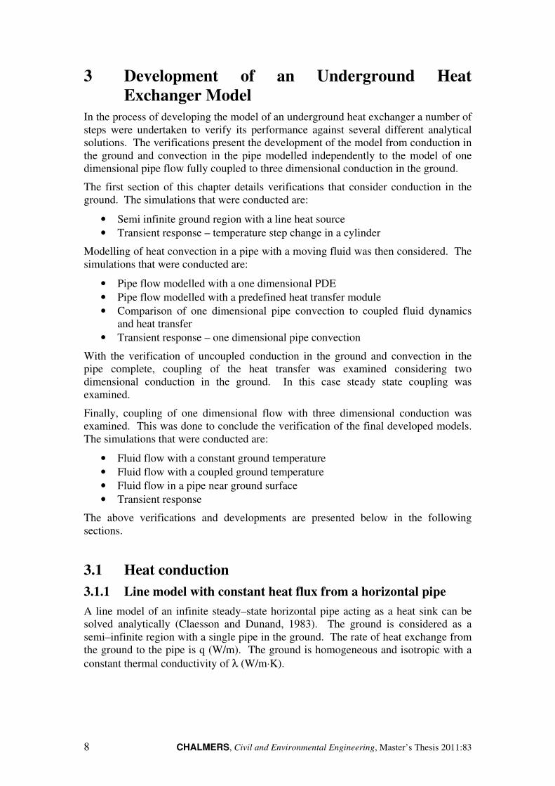
In COMSOL a three dimensional cylinder was constructed as shown in Figure 3.5.
The cylinder was simulated as a solid object with only heat transfer by conduction.
This was done just to test the transient solvers in COMSOL.
Figure 3.6 shows a comparison of the COMSOL and Analytical solution for the
surface temperature of the cylinder. The results show a good agreement between the
two solutions.
Figure 3.5 Cylinder geometry used in step change simulation.

CHALMERS, Civil and Environmental Engineering, Master’s Thesis 2011:83 13
Figure 3.6 Response of the surface temperature along a long cylinder to a step
change in the inner temperature of the cylinder.
3.2 Heat convection in a pipe
3.2.1 Pipe flow modelled with a one dimensional PDE
COMSOL can be used to solve arbitrary partial differential equations (PDEs) in both
a coefficient and general form. In this section the coefficient form of the partial
differential equation has been used to solve a one dimensional heat transfer problem.
A model was developed to verify COMSOLs modelling of fluid flow in a pipe with
transverse heat flow as described in Section 2.2.2.
In COMSOL, Equation (2.12) was modelled using the coefficient form PDE interface.
Equation (3.5) shows the implementation of this PDE that was used to model a steady
state simulation of the pipe (COMSOL AB, 2008).
%o .X�.�X 7 3o .�.� 7 - · 0*�-� * !� 7 p1 7 k · -� 7 q� ) r (3.5)
The convection equation was modelled by setting k ) �� · �� · ,, q ) "!", and r ) "!","0�1. Note that the heat capacity, ��, and the mass flow rate, �� =, were
both assumed to be constant. Since there was assumed to be negligible conduction in
the pipe fluid, the parameters �, ! and p were all set to zero. Steady state conditions
were also assumed and %o and 3o were also set to zero. This resulted in Equation
(3.6).
0
10
20
30
40
50
60
0 100 200 300 400 500 600 700 800
Tem
pera
ture
[°
C]
Time [s]
Analytical
COMSOL

CHALMERS, Civil and Environmental Engineering, Master’s Thesis 2011:83 14
Equation:
*��M� -, * "!", ) "!","0�1 In COMSOL:
k · -� 7 q� ) r
(3.6)
To compare the COMSOL model with the analytical solution the determination of the
surface resistance !" around the pipe was required. This surface resistance consists of
three components: the surface resistance between the fluid and the pipe, the thermal
resistance of the pipe, and the contact resistance between the ground and the pipe. In
this validation it was assumed that water was flowing through the pipe.
The surface resistance between the water and the pipe can be calculated by
considering the conditions of the flow through the pipe. Realistic flow conditions in
the pipe are shown in Table 3.1. These conditions were found in table of sizing
information on ground heat exchangers (ASHRAE, 2003).
Table 3.1 Flow conditions.
Description Symbol Value Units
diameter of pipe D 0.06 m
velocity of water V 0.14 m/s
density of water $ 1000 kg/m3
heat capacity of fluid Cp 4200 W·s/kg
To determine if the flow was turbulent or laminar flow, Reynolds Number was
calculated using Equation (3.7). The result of 8400 indicated that the flow was
turbulent.
�� ) � · ��� (3.7)
The Nussselt number for turbulent flow was then found using the Dittus and Boetler
relation for heating (Rohsenow, Hartnett, and Cho, 1998) as shown in Equation (3.8).
� ) 0.024 · �%".v · �w".x (3.8)
The convection heat transfer coefficient, !y, was then determined using Equation
(3.9) from the Nussselt number.
� ) !y��#z (3.9)
The resulting heat transfer coefficient was calculated at approximately 700 W/(m2K).

CHALMERS, Civil and Environmental Engineering, Master’s Thesis 2011:83 15
The thermal resistance of the pipe was calculated using Equation (3.10) and then
inverted to find the heat transfer coefficient (Claesson and Dunand, 1983).
{�z ) 12V#� ln 4���F5 (3.10)
The ability of the ground to remove heat from the area around the pipe was assumed
to infinite. This assumption was made in order to simulate a larger temperature drop
along the length of the pipe. This was done to make the comparison between the
COMSOL simulation and the analytical solution easier to visualize.
Using the PDE interface in COMSOL and solving the equation as shown in Equation
(3.6) a validation of COMSOL was accomplished. The results of this are shown in
Figure 3.7. This shows an exact match between the analytical and COMSOL results.
Figure 3.7 Comparison of the analytical solution to COMSOL’s PDE interface
solution for flow in a channel with transverse heat loss.
3.2.2 Pipe flow modelled using a predefined heat transfer module
The heat transfer module in COMSOL is designed for heat transfer by conduction,
convection, and radiation. This allows for the simulation of heat transfer in gases,
liquids, and solids. The heat transfer in fluids module allows for simulation of
conduction and convection in a moving fluid. Equation (2.15) shows the differential
equation for heat transfer in fluids. Using the same parameters as in Section 3.2.1
steady–state transverse heat loss in a pipe was simulated using COMSOL. The
results, shown in Figure 3.8, indicate an exact match with the analytical solution.
0
10
20
30
40
50
60
0 20 40 60 80 100
Tem
per
atu
re
[°
C]
Location along pipe [m]
Analytical
COMSOL-PDE

CHALMERS, Civil and Environmental Engineering, Master’s Thesis 2011:83 16
Figure 3.8 Comparison of an analytical solution to COMSOL’s heat transfer
interface solution for flow in a channel with transverse heat loss.
3.2.3 Coupled fluid dynamics and heat transfer
To analyze the transverse heat transfer from the fluid in the pipe to the ground several
simulation were attempted in COMSOL using the interface for coupled heat transfer
and turbulent flow. In COMSOL this model is called ‘Conjugate Heat Transfer’ and
is part of COMSOL’s CFD Module. Full details of the CFD Module can be found in
the COMSOL CFD Module User’s Guide (COMSOL AB, 2008). Some theoretical
background regarding the modelling of the fluid dynamics is shown below.
Fluid flow in the pipe has been modelled using the � * ε turbulence model. This
model introduces two transport equations and two dependent variables:
• k, the turbulent kinetic energy, and
• ε, the dissipation rate of turbulence energy.
Turbulent viscosity is modelled by Equation (3.11).
�8 ) ρ�� kXε (3.11)
where,
Cµ is a model constant.
The transport equation for k is shown below in Equation (3.12).
0
10
20
30
40
50
60
0 20 40 60 80 100
Te
mp
era
ture
[°
C]
Location along pipe [m]
Analytical
COMSOL - Heat Transfer

CHALMERS, Civil and Environmental Engineering, Master’s Thesis 2011:83 17
ρ .�.� 7 ρR · -k ) - · �4µ 7 µ�σ�5 -k� 7 P� * ρε (3.12)
Where the production term is as indicated below in Equation (3.13).
P� ) µ� 4-R: 0-R 7 0-R1�1 * 23 0- · R1X5 * 23 ρk- · R (3.13)
Equation (3.14) shows the transport equation for ε.
ρ .�.� 7 ρR · -ε ) - · �4µ 7 µ�σ�5 -ε� 7 C�Z εk P� * C�Xρ εXk (3.14)
As a validation of the one dimensional channel flow simulation shown in Section
2.2.2, an axisymetric model of a 50 m length of pipe with a constant temperature
boundary conditions was assembled. The geometry of the model is shown in Figure
3.9. In order to limit the size and number of elements in the model, it included only
the fluid in the pipe and the pipe itself. The temperature around the outer edge of the
pipe was assumed to be constant. This was done to match the assumption of constant
ground temperature made in the channel flow simulations above.
In COMSOL the ‘Conjugate Heat Transfer Interface’ is set up to model heat transfer
through a fluid in collaboration with a solid where heat is transferred by conduction.
The interface for conjugate heat transfer includes models for turbulent flow including
fast moving fluids that have a high Reynolds number. This interface also adds
functionality for calculating the dispersion of heat transfer due to turbulence. This is a
complex model that was used to validate the much simpler one dimensional pipe flow
model.
The temperature in the water along the centre of the pipe is compared to the one
dimensional analytical solution as shown in Figure 3.10. The results show a
reasonably close agreement between the two solutions. The two dimensional,
axisymetric model shows a short flat section where the turbulent flow develops
followed by a slightly larger decrease in temperature along the length of the pipe. The
analytical model appears to show a smaller decrease in temperature, but does provide
a good model for pipe flow.

CHALMERS, Civil and Environmental Engineering, Master’s Thesis 2011:83 18
Figure 3.9 Geometry of axisymetric pipe simulated using the ‘Conjugate Heat
Transfer’ interface.
Figure 3.10 Steady–state comparison of three dimensional conjugate heat transfer
and one dimensional channel flow.
0
10
20
30
40
50
60
0 10 20 30 40 50
Te
mp
era
ture
[°
C]
Location along pipe [m]
Analytical
COMSOL - Conjugate Heat Transfer (2D Axisymetric)
CHALMERS, Civil and Environmental Engineering, Master’s Thesis 2011:83 19
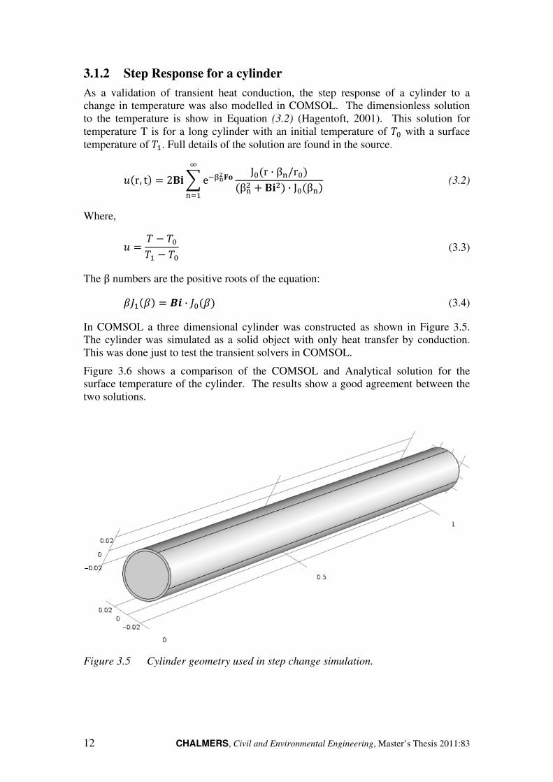
3.2.4 Transient simulation of one dimensional fluid flow
A transient simulation was attempted to validate the performance of COMSOL in a
one dimensional pipe as it responds simply to a step change in the temperature of the
water at the inlet. This simulation assumed no transverse heat transfer along the
length of the pipe and no conduction in the pipe fluid. The fluid in the pipe was
initially at 12 °C. At time zero the water at the inlet was changed to 50 °C. Due to
the step change in the inlet temperature, a hot wave should move down the pipe until
the temperature in the entire pipe is 50 °C.
When using COMSOL’s default time dependent solver, oscillation in the solved
temperature were observed as shown in Figure 3.11. To reduce the oscillations and
improve the accuracy of the simulations, several modifications were made in
COMSOL. These changes included reduction of the time step, reduction in the
element size, and reduction of the tolerance of the solver.
COMSOL also has an additional feature for handling numerical instabilities within the
heat transfer interface. One of the techniques is to add terms to the transport
equations. This is termed artificial diffusion and can be used to stabilize the solution.
Details of the methods can be found in the COMSOL documentation (COMSOL AB,
2008). With artificial diffusion the oscillations can be controlled as shown in Figure
3.12. The general performance of the simulation is similar to an exact step change.
There is, however, some smoothing of the transition from the initial to inlet
temperature of the pipe. The impact of this will be relatively small, since the
simulated response, on average, is similar to the exact solution.
Figure 3.11 Transient simulation of convective heat flow responding to a step
change in the inlet temperature using COMSOL’s default solver.
0
10
20
30
40
50
60
70
0 50 100 150 200
Tem
per
atu
re [°C
]
Location along pipe [m]
0
300
600
900
1200
1500
Time [s]

CHALMERS, Civil and Environmental Engineering, Master’s Thesis 2011:83 20
Figure 3.12 Transient simulation of convective heat flow responding to a step
change in the inlet temperature with solver stabilization.
A second transient simulation of a one dimensional pipe as it responds to a step
change in the temperature of the water at the inlet was conducted. In this simulation
transverse heat transfer along the length of the pipe was considered. Heat loss to a
medium at constant temperature was used. The fluid in the pipe was initially at 12 °C.
At time zero the water at the inlet was changed to 50 °C. The results of this
simulation are shown in Figure 3.13. These results show that as the fluid flow
through the pipe, the temperature changes from the initial ground temperature to the
steady state temperature solution as shown in Figure 3.8.
0
10
20
30
40
50
60
0 50 100 150 200
Tem
per
atu
re [°C
]
Location along pipe [m]
100
100 - Exact
500
500 - Exact
900
900 - Exact
1300
1300 - Exact
Time [s]

CHALMERS, Civil and Environmental Engineering, Master’s Thesis 2011:83 21
Figure 3.13 Transient simulation of convective heat flow responding to a step
change in the inlet temperature from an initial colder ground
temperature.
In order to examine the periodic response of the temperatures in the pipe, a model was
examined with a periodically varying temperature at the inlet of the pipe. The
temperature in the surrounding pipe was assumed to be constant at a temperature of
12 °C. This was also the initial temperature for both the ground and the pipe. The
inlet temperature, ,F, varied according to Equation (3.15) with a mean inlet
temperature, ,��oG, of 50 °C, an amplitude, ,o��, of 10 °C, a time period, ��, of one
hour, and with zero time delay, ��.
,F ) ,��oG 7 ,o�� · sin �2 · V · 0� * ��1�� � (3.15)
The general response of the temperature in the pipe to the varying inlet temperature is
show in Figure 3.14. The resulting temperature response at the outlet of the pipe
formed a regular periodic function as shown in Figure 3.15. There is a reduction in
the mean temperature and amplitude as well as a time delay when compared to the
original inlet temperature. The time delay is 1430 s, the time it takes for water to
move from the inlet to the outlet based on an average velocity of 0.14 m/s.
0
10
20
30
40
50
60
0 50 100 150 200
Tem
per
atu
re [°C
]
Location along pipe [m]
0
300
600
900
1200
1500
Time [s]

CHALMERS, Civil and Environmental Engineering, Master’s Thesis 2011:83 22
Figure 3.14 Periodic transient simulation of convective heat flow responding to a
periodic inlet temperature from an initial colder ground temperature.
Figure 3.15 Time response of the temperature at the pipe boundaries subject to a
periodically varying inlet temperature from an initial colder ground
temperature.
0
10
20
30
40
50
60
70
0 50 100 150 200
Tem
per
atu
re [°C
]
Location along pipe [m]
0
400
800
1200
1600
2000
2400
Time [s]
0
10
20
30
40
50
60
70
0 1000 2000 3000 4000 5000 6000 7000 8000
Tem
per
atu
re [
C]
Time[s]
x=0
x=200
Periodic Equation

CHALMERS, Civil and Environmental Engineering, Master’s Thesis 2011:83 23
3.3 Two dimensional conduction coupled to one
dimensional convection
With separate verifications of conduction in the ground and convection in the pipe
complete, coupling of the heat transfer was examined. The first coupled simulation,
presented here, considers two dimensional conduction in the ground with one
dimensional convection in the pipe. The development of a two dimensional model
was achieved using linear extrusion coupling as described in Section 2.3. In this
simulation steady state coupling was examined.
A simple pipe through a two dimensional domain was developed as shown in Figure
3.16. A separate one dimensional model of the pipe was also developed. It is shown
in Figure 3.17. In order to couple the two models, an edge extrusion variable was first
used in the model of the ground. This variable is mapped to a source, which is the
line in the ground representing the pipe. The destination for this variable is then
specified as the line in the pipe model. The corresponding extrusion variable for the
temperature of the fluid in the pipe is mapped in the same way to the line in the
ground. The heat transfer between the pipe and the ground was then modelled with
the following equation.
q ) "!"�,"0�1 * ,0�1� (3.16)
In COMSOL this heat transfer from the pipe to the ground is automatically calculated
for each time step and for each element in the simulation.
Figure 3.16 Model of the ground in a two dimensional domain.
CHALMERS, Civil and Environmental Engineering, Master’s Thesis 2011:83 24
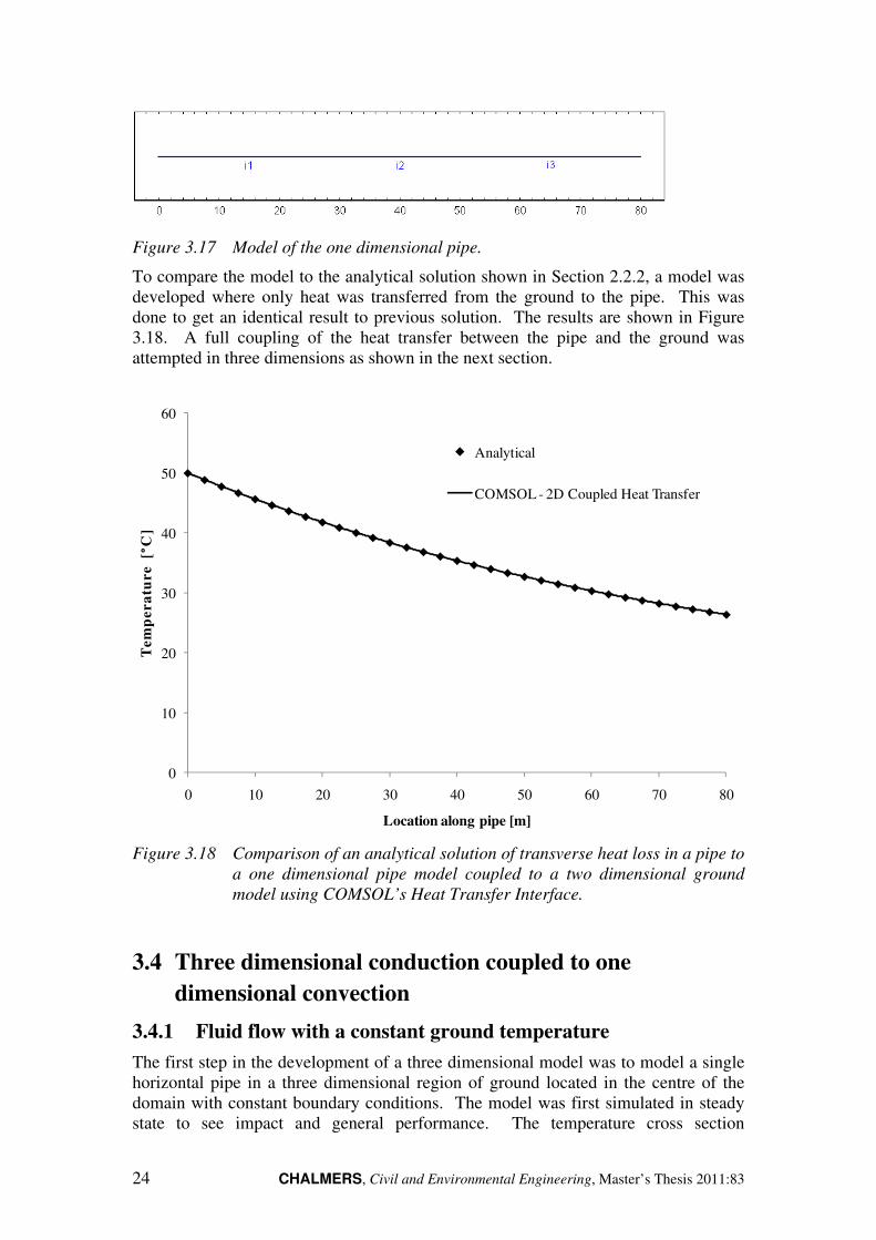
Figure 3.17 Model of the one dimensional pipe.
To compare the model to the analytical solution shown in Section 2.2.2, a model was
developed where only heat was transferred from the ground to the pipe. This was
done to get an identical result to previous solution. The results are shown in Figure
3.18. A full coupling of the heat transfer between the pipe and the ground was
attempted in three dimensions as shown in the next section.
Figure 3.18 Comparison of an analytical solution of transverse heat loss in a pipe to
a one dimensional pipe model coupled to a two dimensional ground
model using COMSOL’s Heat Transfer Interface.
3.4 Three dimensional conduction coupled to one
dimensional convection
3.4.1 Fluid flow with a constant ground temperature
The first step in the development of a three dimensional model was to model a single
horizontal pipe in a three dimensional region of ground located in the centre of the
domain with constant boundary conditions. The model was first simulated in steady
state to see impact and general performance. The temperature cross section
0
10
20
30
40
50
60
0 10 20 30 40 50 60 70 80
Te
mp
era
ture
[°
C]
Location along pipe [m]
Analytical
COMSOL - 2D Coupled Heat Transfer

CHALMERS, Civil and Environmental Engineering, Master’s Thesis 2011:83 25
perpendicular to the pipe can then be compared to the temperature distributions
obtained in Section 3.1.1 based on an assumption of a constant temperature cross
section. The geometry of the pipe and the ground can be seen below in Figure 3.19.
Figure 3.19 Geometry of the three dimensional simulation.
The results of the simulation, when compared to the analytical solution from Equation
(2.13) are shown in Figure 3.20. The agreement between the simulation and the
analytical solution, as in previous cases, is very good. This indicates that the one
dimensional pipe flow model is able to simulate the heat transfer from the pipe to the
ground with sufficient accuracy.

CHALMERS, Civil and Environmental Engineering, Master’s Thesis 2011:83 26
Figure 3.20 Comparison of an analytical solution of transverse heat loss in a pipe to
a one dimensional pipe model coupled to a three dimensional ground
model with constant ground temperature using COMSOL’s Heat
Transfer Interface.
3.4.2 Fluid flow with a coupled ground temperature
An attempt was made to validate the full coupling between the fluid flow in the pipe
and the ground. This was accomplished by constructing a two dimensional
axisymetric model in COMSOL using the heat transfer interface. An 800 m long pipe
was simulated with the geometry as shown in Figure 3.. Water flowed along the pipe
at a rate of 0.14 m/s. The flow turbulence was not modelled. The conduction of the
water in the radial direction was assumed to be very high to model heat transfer
towards the ground. The purpose of this validation was to verify the full coupling
between the heat transfer in the pipe with the heat transfer in the ground. The
geometry of the three dimensional model is shown in Figure 3.22.
0
10
20
30
40
50
60
0 20 40 60 80 100
Te
mp
er
atu
re [°
C]
Location along pipe [m]
Analytical
COMSOL-3D Constant Tsoil

CHALMERS, Civil and Environmental Engineering, Master’s Thesis 2011:83 27
Figure 3.21 Geometry of the two dimensional axisymetric simulation.
Figure 3.22 Geometry of a three dimensional, fully coupled model with a pipe in the
centre of the ground.
The results from the comparison between the two models are shown in Figure 3.23.
There appears to be a reasonable agreement between the two models. It appears that
water
pipe
ground
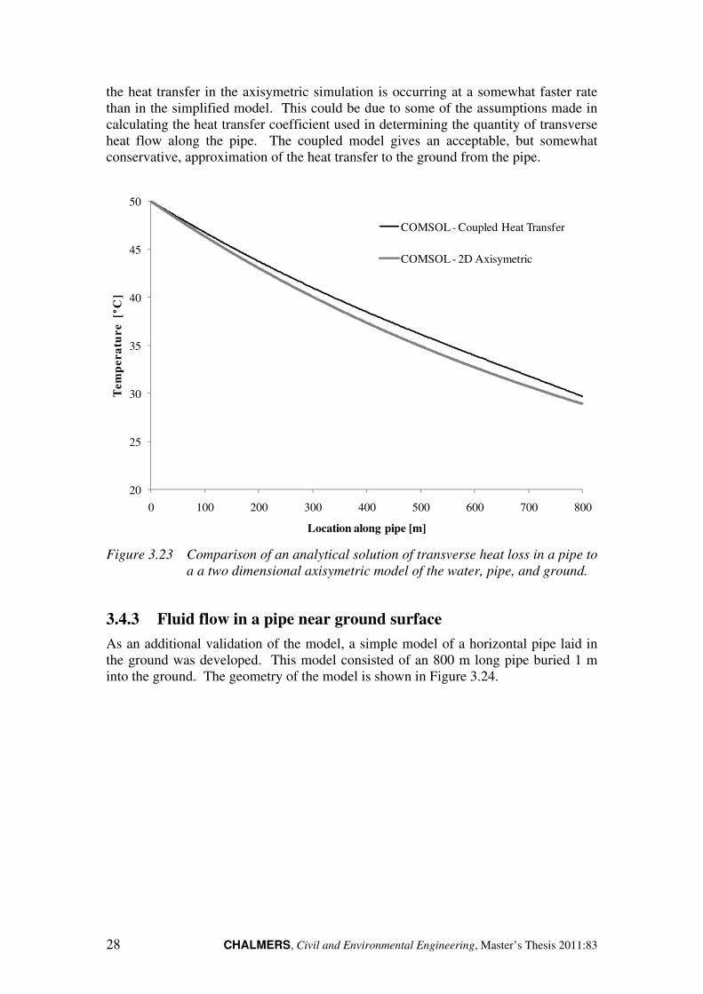
CHALMERS, Civil and Environmental Engineering, Master’s Thesis 2011:83 28
the heat transfer in the axisymetric simulation is occurring at a somewhat faster rate
than in the simplified model. This could be due to some of the assumptions made in
calculating the heat transfer coefficient used in determining the quantity of transverse
heat flow along the pipe. The coupled model gives an acceptable, but somewhat
conservative, approximation of the heat transfer to the ground from the pipe.
Figure 3.23 Comparison of an analytical solution of transverse heat loss in a pipe to
a a two dimensional axisymetric model of the water, pipe, and ground.
3.4.3 Fluid flow in a pipe near ground surface
As an additional validation of the model, a simple model of a horizontal pipe laid in
the ground was developed. This model consisted of an 800 m long pipe buried 1 m
into the ground. The geometry of the model is shown in Figure 3.24.
20
25
30
35
40
45
50
0 100 200 300 400 500 600 700 800
Tem
pe
ra
tur
e [°
C]
Location along pipe [m]
COMSOL - Coupled Heat Transfer
COMSOL - 2D Axisymetric

CHALMERS, Civil and Environmental Engineering, Master’s Thesis 2011:83 29
Figure 3.24 Geometry of a three dimensional, fully coupled model with a pipe at a
depth of 1 m in the ground.
During this validation an analytical solution was compared to the numerical
simulation results. The equation for the analytical solution was the same as used in
Equation (2.13). The only difference was in the calculation of α". An equivalent
thermal resistance of the ground was added to heat transfer coefficient. The
calculation of this was based on an equation for the resistance of a pipe buried in the
ground (Claesson and Dunand, 1983). The additional transfer coefficient, α>, is
calculated with:
α> ) ��·�hCc·�� D (3.17)
With this additional transfer coefficient accounted for in the analytical solution a close
match is developed to the COMSOL model. The result is shown in Figure 3.25

CHALMERS, Civil and Environmental Engineering, Master’s Thesis 2011:83 30
Figure 3.25 Comparison of an analytical solution of transverse heat loss in a pipe to
a one dimensional pipe model coupled to a three dimensional ground
model with a coupled ground temperature.
The above simulation was done along an 800 m long domain. It had a depth and
width of 60 m. In order to assess the required domain size around the pipe a
parametric study was conducted where the depth and width were varied from 20 to 80
m with a step size of 20 m. The results of this study are shown in Figure 3.26 and
Figure 3.27. These show almost no effect on the temperature distribution in the pipe
as the width and depth of the domain is increased above 20 m. Figure 3.26 shows that
each of the domain sizes yielded identical results. Figure 3.27 shows the results from
the 20 and 40 m size domain. The results for the 60 and 80 m size domain were the
same as those from 40 m. Based on this result, future simulations will use a similar
domain size.
0
10
20
30
40
50
60
0 100 200 300 400 500 600 700 800 900
Te
mp
era
tur
e
[°C
]
Location along pipe [m]
Analytical
COMSOL - Coupled Heat Transfer

CHALMERS, Civil and Environmental Engineering, Master’s Thesis 2011:83 31
Figure 3.26 Comparison of domain size in a one dimensional pipe model fully
coupled to a three dimensional ground mode.
Figure 3.27 Temperature distribution at x=10 m along the centre of the pipe with
various domain sizes.
20
25
30
35
40
45
50
0 100 200 300 400 500 600 700 800
Tem
pera
ture [°
C]
Location along pipe [m]
20
40
60
80
10
12
14
16
18
20
22
24
26
28
30
0 5 10 15 20
Tem
pera
ture [°
C]
Depth below soil [m]
20
40
CHALMERS, Civil and Environmental Engineering, Master’s Thesis 2011:83 32
3.4.4 Transient performance of the model
Two simple analyses were conducted to examine the transient performance of the pipe
flow in the fully coupled ground. The analyses involved a step and periodical change
in the inlet temperature of the pipe. The temperature at the boundaries of the ground
was assumed to be constant.
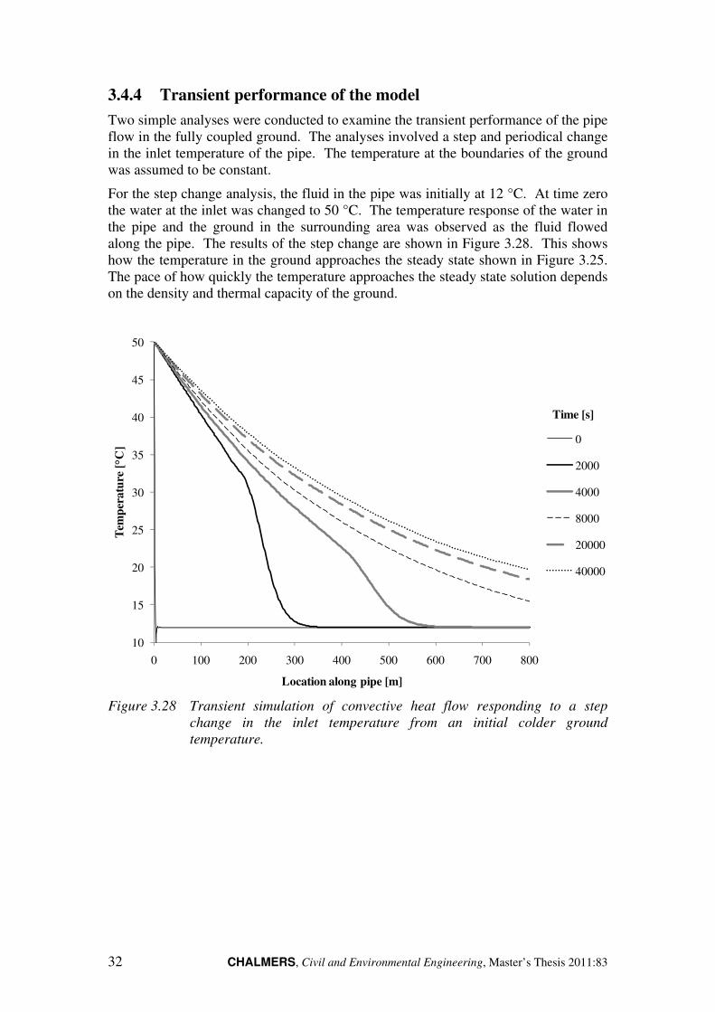
For the step change analysis, the fluid in the pipe was initially at 12 °C. At time zero
the water at the inlet was changed to 50 °C. The temperature response of the water in
the pipe and the ground in the surrounding area was observed as the fluid flowed
along the pipe. The results of the step change are shown in Figure 3.28. This shows
how the temperature in the ground approaches the steady state shown in Figure 3.25.
The pace of how quickly the temperature approaches the steady state solution depends
on the density and thermal capacity of the ground.
Figure 3.28 Transient simulation of convective heat flow responding to a step
change in the inlet temperature from an initial colder ground
temperature.
10
15
20
25
30
35
40
45
50
0 100 200 300 400 500 600 700 800
Tem
per
atu
re [°C
]
Location along pipe [m]
0
2000
4000
8000
20000
40000
Time [s]

CHALMERS, Civil and Environmental Engineering, Master’s Thesis 2011:83 33
4 Models of Underground Heat Exchangers
Several models were completed in COMSOL of the underground heat exchangers.
Models of both horizontal pipes and borehole exchangers have been developed. This
chapter describes each of the models. This chapter also describes the process of
converting the underground heat exchanger model into an S–function for use in
Simulink. Finally, the response of the BHE model to a step changes in the inlet
temperature of the fluid flowing through the system is also examined using the
developed S–functions.
4.1 The COMSOL models
4.1.1 Single linear horizontal pipe
The first model created was of a single horizontal pipe in the ground. The pipe is
modelled as a straight pipe at a constant depth in the ground. The model can also be
used to simulate any horizontal pipe placed at a constant depth in the ground where
curves or elbows in the pipe or additional pipes do not have a significant effect on
each other. For example, an entire horizontal pipe loop could be simulated if
segments of the loop do not thermally interact with other segments. The model could
also be modified, however, to be used in other configurations of horizontal pipes.
Figure 4.1 Final model of a horizontal underground heat exchanger.
The model allows the user to input a number of different properties and parameters as
variables in the model. These values include the characteristics of the pipe, the initial
temperatures in the domains, and the thermal characteristics of the ground. A full list
of the properties and variables that the user can enter are shown in Table 4.1.

CHALMERS, Civil and Environmental Engineering, Master’s Thesis 2011:83 34
Table 4.1 List of global constants for horizontal underground heat exchanger.
Input Variable Description Units
L0 Inner circumference of the pipe m
alpha0 Heat transfer coefficient from fluid to ground W/(m2·K)
Tgin Initial ground temperature °C
Ti Initial inlet temperature of the pipe °C
xarea Cross sectional area of the pipe °C
flow_velocity Velocity of the fluid in the pipe m/s
Tsoiltop Initial exterior temperature at ground surface °C
Tsoilbottom Initial and long term temperature of ground °C
k_ground Conductivity of the ground W/(m·K)
rho_ground Density of the ground kg/m3
cp_ground Heat Capacity of the ground J/(kg·K)
k_fluid Conductivity of the pipe fluid W/(m·K)
rho_fluid Density of the pipe fluid kg/m3
cp_fluid Heat Capacity of the pipe fluid J/(kg·K)
The model of the ground considers conduction through the ground using the thermal
characteristics of k_ground, rho_ground, and cp_ground. The ground is assumed to
be isotropic with a constant density and heat capacity throughout. The model could
be modified, however, to consider variation in these properties within the ground to
model different layers of soil and rock. The model, as mentioned previously, also
assumes there is no diffusion of water within the ground.
Adiabatic boundary conditions are used along all of the boundaries of the ground
except for the top and bottom. The space around the pipe domain was selected such
that the adiabatic boundary conditions can accurately represent real situations. A
distance of 20 m was chosen based on the results obtained from Section 3.4.3. The
top and bottom boundary both have a temperature specified at the boundary. The
variables Tsoiltop and Tsoilbottom are used to input the top and bottom temperature,
respectively. The top temperature is the outdoor dry bulb temperature while the
bottom temperature is the long term average temperature of the ground.
The model of the pipe consists simply of a one–dimensional line with a length, in this
case, of 200 m as shown in Figure 4.2. The model of the pipe considers only
convection in the pipe using the thermal characteristics of k_fluid, rho_fluid, and

CHALMERS, Civil and Environmental Engineering, Master’s Thesis 2011:83 35
cp_fluid. The velocity of the fluid in the pipe is assumed to be constant at a rate of
flow_velocity. Since only convection is being simulated only one boundary condition
must be specified. In this case the temperature at the inlet (x=0) is specified. The
return temperature is calculated during the simulations.
Figure 4.2 Linear model of a horizontal pipe.
4.1.2 Single loop BHE
The BHE is modelled using a three dimensional model of the ground with a
cylindrical borehole in the centre. The pipe is modelled as two straight pipe segments
running vertically through the borehole. One segment represents the flow in the pipe
running down to the bottom and the other segment represents the fluid returning.
Figure 4.3 shows the model of the ground with the borehole.
Figure 4.3 Model of the ground and the single loop BHE.
This model, as with the horizontal pipe model, allows the user to input a number of
different properties and parameters as variables in the model. The values input are the
same as for the horizontal pipe, with the addition of specifying the characteristics of
the grout or filler material used within the borehole. A full list of the properties and

CHALMERS, Civil and Environmental Engineering, Master’s Thesis 2011:83 36
variables that the user can enter are shown in Table 4.2. The boundary conditions of
the ground are identical to those described in the section above.
Table 4.2 List of global constants for the BHE models.
Input Variable Description Units
L0 Inner circumference of the pipe m
alpha0 Heat transfer coefficient from fluid to ground W/(m2·K)
Tgin Initial ground temperature °C
Ti Initial inlet temperature of the pipe °C
xarea Cross sectional area of the pipe °C
flow_velocity Velocity of the fluid in the pipe m/s
Tsoiltop Initial exterior temperature at ground surface °C
Tsoilbottom Initial and long term temperature of ground °C
k_ground Conductivity of the ground W/(m·K)
rho_ground Density of the ground kg/m3
cp_ground Heat capacity of the ground J/(kg·K)
k_grout Conductivity of the grout W/(m·K)
rho_grout Density of the grout kg/m^3
cp_grout Heat Capacity of the grout J/(kg·K)
k_fluid Conductivity of the pipe fluid W/(m·K)
rho_fluid Density of the pipe fluid kg/m3
cp_fluid Heat Capacity of the pipe fluid J/(kg·K)
4.1.3 Models of multiple single loop BHEs
Several COMSOL models with multiple boreholes were developed to verify the
performance of more complex models. For example, a model with four boreholes was
developed as shown in Figure 4.4. This model was developed in the same way as the
single U–pipe model. There is, however, a separate model for each pipe. In this
study they are assumed to be operating in parallel.

CHALMERS, Civil and Environmental Engineering, Master’s Thesis 2011:83 37
Figure 4.4 Model of the ground and four BHE systems.
An infinite array of BHE can also be modelled. The model is nearly identical to the
single BHE shown in the previous section. The only difference is the spacing around
the borehole. The boundaries of the simulation will be at the midpoint between the
adjacent boreholes. For example, consider an array of boreholes, similar to what is
shown in Figure 4.5, have a spacing of x m between them. In this case the same
model of a single BHE, shown in the previous section, can be used. The only
difference is the space around the borehole in the x and y direction would be equal to
half the distance between the boreholes.

CHALMERS, Civil and Environmental Engineering, Master’s Thesis 2011:83 38
Figure 4.5 Top view of a sample array of BHEs.
4.2 Simulink and S–Functions
In order to simulate complex building models, the Simulink program was used.
Simulink is a program for the simulation of time varying and embedded systems. It
provides an interactive graphical environment that is integrated into Matlab. The
graphical environment allows development of models using something similar to flow
diagrams.
In Simulink S–Functions can be used to interact with complex functions written in
various programming environments. In the Matlab documentation an S–Function is
described as:
S–functions (system–functions) provide a powerful mechanism for extending
the capabilities of the Simulink environment. An S–function is a computer
language description of a Simulink block written in MATLAB®
, C, C++, or
Fortran.
In these simulations Level 2 S–functions were used. Level 2 S–functions allow
functions to be written in MATLAB that can interact with the Simulink environment
in a highly customizable fashion.
Using these S–functions, COMSOL simulations can be integrated into a Simulink
block. In COMSOL, there is an interface for incorporating simulations into Matlab
functions. The COMSOL models are simply saved as a model m–file which allows
them to be run in Matlab.
4.2.1 A simple embedded model using a S–function
A simple model was developed in COMSOL, converted to an m–file, and integrated
into an S–function. This S–function was then used in a Simulink model which is
shown in Figure 4.6. This model was developed simply for the purpose of testing the
functionality of Simulink and COMSOL integration.
x [m]

CHALMERS, Civil and Environmental Engineering, Master’s Thesis 2011:83 39
Figure 4.6 Simple Simulink model including an embedded S–function that invokes
a COMSOL model.
The model created in COMSOL was a simple model of one dimensional heat flow.
After being developed, it was then saved as a model m–file. This model m–file is
written in Matlab script and it can be directly run using MATLAB. The S–function,
heat1Dsfun, was developed from this m–file in the required format. The code for the
function, which shows the form of the S–function, is shown in Figure 4.6. This code
shows the required function blocks that are needed to create a Level–2 m–file. It
includes the functions Setup, Update, and Output. The purpose of each of these
functions in the context of running a transient COMSOL simulation is as follows:
• Setup. This function initiates the setup of the S–function, including the code
for the creation of the COMSOL model.
• Update. This function updates the COMSOL model during each time–step in
the Simulink simulation. For example, any new boundary conditions are
applied to the model and the simulation is run until the next time step.
• Output. In this function, any desired outputs from the COMSOL simulation
are output to the Simulink simulation.
Full details of the Level–2 S–functions can be found in the MATLAB documentation
(MathWorks, Inc., 1984). The full code for the setup and updating of the heat1Dsfun
simulation can be found in Appendix A.
Sine Wave
Scope
heat1Dsfun
Level-2 M-file
S-Function

CHALMERS, Civil and Environmental Engineering, Master’s Thesis 2011:83 40
Figure 4.7 Matlab S–function showing function block set–up. (Note that the code
to initialize and update the COMSOL simulation has been removed).
4.3 S–Functions of underground heat exchangers
The procedure and format, as described in the previous section was used to integrate
full COMSOL models of underground heat exchangers into Simulink models of
buildings. This section describes each of the S–functions that were developed.
4.3.1 Single linear horizontal pipe
A Level 2 S–function of the horizontal pipe model was developed similar to the
simple S–function developed in the previous section. The model developed in section
4.1.1 was saved as a model m–file and then programmed as part of a dynamic S–
function. The function consists of the main model m–file, ‘SinglePipeHoriz_sfun.m’,
along with a separate file containing a list of constants and parameters. This file is
named ‘SinglePipeHoriz_constants.m’. It contains details such as the characteristics
of the pipe, the thermal properties of all the materials, parameters relating to the size
of the mesh, and an option to output the temperature in the ground to a separate file.
The full list of constants and parameters contained in this file are shown in Table 4.3.
function heat1Dsfun(block) % Level-2 M file S-Function demonstrating integration of a COMSOL model. setup(block); %endfunction
function setup(block) %% Register number of input and output ports block.NumInputPorts = 1; block.NumOutputPorts = 1; %% Setup functional port properties to dynamically %% inherited. block.SetPreCompInpPortInfoToDynamic; block.SetPreCompOutPortInfoToDynamic; block.InputPort(1).DirectFeedthrough = true; %% Set block sample time to inherited block.SampleTimes = [-1 0]; %% Set the block simStateCompliance to default (i.e., same as a built-in block) block.SimStateCompliance = 'DefaultSimState'; %% Run accelerator on TLC block.SetAccelRunOnTLC(false); %% Register methods block.RegBlockMethod('PostPropagationSetup', @DoPostPropSetup); block.RegBlockMethod('Outputs', @Output); block.RegBlockMethod('Update', @Update); %%%%%%%%%%%%%%%%%%%%%%%%%%%%%%%%%%%%%%%%%%%%%%%% global fem global tout global solut %%%%%%%%%%%%%%%%%%%%%%%%%%%%%%%%%%%%%%%%%%%%%%%%% % Initialize COMSOL Simulations %%% %%%%%%%%%%%%%%%%%%%%%%%%%%%%%%%%%%%%%%%%%%%%%%%%
function Update(block) %%%%%%%%%%%%%%%%%%%%%%%%%%%%%%%%%%%%%%%%%%%%%%%%% % Update COMSOL Simulations %%% %%%%%%%%%%%%%%%%%%%%%%%%%%%%%%%%%%%%%%%%%%%%%%%% %endfunction
function Output(block) global tout block.OutputPort(1).Data = tout; %endfunction

CHALMERS, Civil and Environmental Engineering, Master’s Thesis 2011:83 41
Table 4.3 List of static parameters and simulation variables in
SinglePipeHoriz_constants.m file.
Input Variable Description Units
Static Parameters
horiz_pipe.pipelength Length of pipe m
horiz_pipe.pipedepth Depth of pipe from ground surface m
horiz_pipe.soilspace Space of ground around the pipe in all
horizontal directions and in depth
m
Simulation Variables
horiz_pipe.L0 Inner circumference of the pipe m
horiz_pipe.alpha0 Heat transfer coefficient from fluid to
ground
W/(m2·K)
horiz_pipe.Tgin Initial ground temperature °C
horiz_pipe.Ti Initial inlet temperature of the pipe °C
horiz_pipe.xarea Cross sectional area of the pipe °C
horiz_pipe.flow_velocity Velocity of the fluid in the pipe m/s
horiz_pipe.Tsoiltop Initial exterior temperature at ground
surface
°C
horiz_pipe.Tsoilbottom Initial and long term temperature of
ground
°C
horiz_pipe.k_ground Conductivity of the ground W/(m·K)
horiz_pipe.rho_ground Density of the ground kg/m3
horiz_pipe.cp_ground Heat capacity of the ground J/(kg·K)
horiz_pipe.k_grout Conductivity of the grout W/(m·K)
horiz_pipe.rho_grout Density of the grout kg/m^3
horiz_pipe.cp_grout Heat Capacity of the grout J/(kg·K)
horiz_pipe.k_fluid Conductivity of the pipe fluid W/(m·K)
horiz_pipe.rho_fluid Density of the pipe fluid kg/m3
horiz_pipe.cp_fluid Heat capacity of the pipe fluid J/(kg·K)
CHALMERS, Civil and Environmental Engineering, Master’s Thesis 2011:83 42
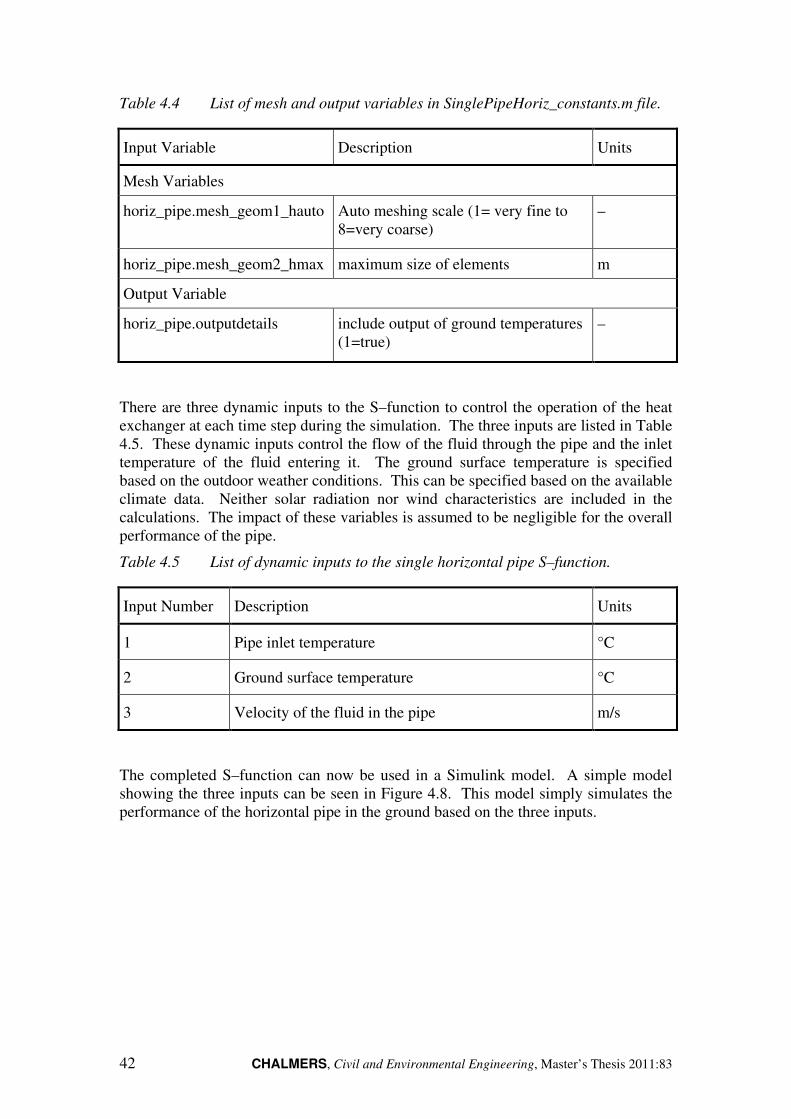
Table 4.4 List of mesh and output variables in SinglePipeHoriz_constants.m file.
Input Variable Description Units
Mesh Variables
horiz_pipe.mesh_geom1_hauto
Auto meshing scale (1= very fine to
8=very coarse)
–
horiz_pipe.mesh_geom2_hmax maximum size of elements m
Output Variable
horiz_pipe.outputdetails
include output of ground temperatures
(1=true)
–
There are three dynamic inputs to the S–function to control the operation of the heat
exchanger at each time step during the simulation. The three inputs are listed in Table
4.5. These dynamic inputs control the flow of the fluid through the pipe and the inlet
temperature of the fluid entering it. The ground surface temperature is specified
based on the outdoor weather conditions. This can be specified based on the available
climate data. Neither solar radiation nor wind characteristics are included in the
calculations. The impact of these variables is assumed to be negligible for the overall
performance of the pipe.
Table 4.5 List of dynamic inputs to the single horizontal pipe S–function.
Input Number Description Units
1 Pipe inlet temperature °C
2 Ground surface temperature °C
3 Velocity of the fluid in the pipe m/s
The completed S–function can now be used in a Simulink model. A simple model
showing the three inputs can be seen in Figure 4.8. This model simply simulates the
performance of the horizontal pipe in the ground based on the three inputs.

CHALMERS, Civil and Environmental Engineering, Master’s Thesis 2011:83 43
Figure 4.8 Simulink model including an embedded S–Function of the horizontal
pipe model.
4.3.2 Models of BHEs
Several models of various configurations of BHEs were also developed. These
models were developed in order to be able to quantify the performance of several
different types of BHEs. The S–functions that were created are shown in Table 4.6.
Table 4.6 List of S–functions created for modeling BHEs.
S–function filename Type of System Modelled Constants File
InfSingleUpipe_sfun.m Single or infinite array of
boreholes
InfSingleUpipe_constants.m
Upipe_124_sfun.m Model of one, two, or four
boreholes
Upipe_124_constants.m
Upipe_4816_sfun.m Model of four, eight, or
sixteen boreholes
Upipe_4816_constants.m
Each of the three S–functions is linked to a file containing its relevant constants and
parameters as listed in Table 4.6. Similar to the file for the horizontal pipe, the
constants file contains details such as the characteristics of the pipe and the borehole,
the thermal properties of all the materials, parameters relating to the size of the mesh,
and an option to output the temperature in the ground to a separate file. The full list
of constants and parameters contained in this file are shown in Table 4.7. Note that
this file contains the constants that are common to all three of the S–functions.
Constants that only apply to one or two of the functions are indicated in the table.
Sine Wave - Pipe Inlet Temp [°C]
Scope
1
Pipe Inlet Temperature [°C]Manual Switch
SinglePipeHoriz_sfun
Level-2 M-fi le
S-Function9.8
Ground Surface Temperature [°C]
0.6
Fluid Velocity [m/s]

CHALMERS, Civil and Environmental Engineering, Master’s Thesis 2011:83 44
Table 4.7 List of static parameters, mesh variables and the output variable in the
BHE constant files.
Input Variable Description Units
Static Parameters
U_pipe.pipelength Length of pipe m
U_pipe.pipedepth Depth of pipe from ground surface m
U_pipe.soilspace Space of ground around the pipe in all
horizontal directions and in depth
m
U_pipe.boreholediameter Diameter of the borehole m
U_pipe.relativepipelocation Relative location of the pipes in the borehole
compared to the width of the borehole
–
U_pipe.TsoilinitialdegC Initial ground temperature °C
U_pipe. Boreholespace1
Spacing between the boreholes m
U_pipe.nborehole2 Number of boreholes to simulate –
Mesh Variables
U_pipe.mesh_geom1_hauto Auto meshing scale –
U_pipe.mesh_geom2_hmax Maximum size of elements m
Output Variable
U_pipe.outputdetails Include output of ground temperatures
(1=true)
–
Notes:
1. Boreholespace. This applies to all models. If one single borehole is to be simulated
with the InfSingleUPipe model then this value should be equal to the pipespace value.
2. Number of Pipes. Only applies to Upipe148 and Upipe4816 models. In the
Upipe148 only 1,4 and 8 are applicable values and in Upipe4816 only 4,8, and 16 are
applicable.

CHALMERS, Civil and Environmental Engineering, Master’s Thesis 2011:83 45
Table 4.8 List of simulation variables in the BHE constant files.
Input Variable Description Units
Simulation Variables
U_pipe.L0 Inner circumference of the pipe m
U_pipe.alpha0 Heat transfer coefficient from fluid to ground W/(m2·K)
U_pipe.Tgin Initial ground temperature °C
U_pipe.Ti Initial inlet temperature of the pipe °C
U_pipe.xarea Cross sectional area of the pipe °C
U_pipe.flow_velocity Velocity of the fluid in the pipe m/s
U_pipe.Tsoiltop Initial exterior temperature at ground surface °C
U_pipe.Tsoilbottom Initial and long term temperature of ground °C
U_pipe.k_ground Conductivity of the ground W/(m·K)
U_pipe.rho_ground Density of the ground kg/m3
U_pipe.cp_ground Heat Capacity of the ground J/(kg·K)
U_pipe.k_grout Conductivity of the grout W/(m·K)
U_pipe.rho_grout Density of the grout kg/m3
U_pipe.cp_grout Heat Capacity of the grout J/(kg·K)
U_pipe.k_fluid Conductivity of the pipe fluid W/(m·K)
U_pipe.rho_fluid Density of the pipe fluid kg/m3
U_pipe.cp_fluid Heat Capacity of the pipe fluid J/(kg·K)
As with the single horizontal pipe, there are three dynamic inputs to the S–function
which control the operation of the heat exchanger at each time step during the
simulation. The three inputs are the same as those for the horizontal pipe and are
listed in Table 4.5.
The completed S–function can now be used in a Simulink model. A simple model
showing the three inputs can be seen in Figure 4.9. This model simply simulates the
performance of the horizontal pipe in the ground based on the three inputs.

CHALMERS, Civil and Environmental Engineering, Master’s Thesis 2011:83 46
Figure 4.9 Simulink model including an embedded S–function of the BHE model.
4.4 Step response of BHEs
In order to implement a comparison between the different BHEs, it was decided to
compare the performance of each of the models in response to a step change in
temperature. This was done to obtain a simplified response of the heat exchangers as
well as verify their expected performance. The simulations were conducted using the
borehole S–functions ‘InfSingleUpipe_sfun.m’, ‘Upipe_124_sfun.m’, and
‘Upipe_4816_sfun.m’. The tested borehole configurations are shown in Figure 4.10
and listed in Table 4.9.
Each simulation consisted of a ground domain, boreholes, and pipes at an initial
constant temperature of 8 °C. At time zero, the flow through each of the boreholes
begins at a velocity of 0.6 m/s at an inlet temperature of 4°C. In order to compare the
step response between the pipes, the return temperature in the water has been recorded
for one year. In cases with multiple boreholes, the flow through each borehole was
assumed to be in parallel.
Switch
Scope
1
Pipe Inlet T [°C]
Periodic Pipe Inlet T [°C]
InfSingleUpipe_sfun
Level-2 M-file
S-Function9.8
Ground Surface Temperature [°C]
0.6
Fluid Velocity [m/s]
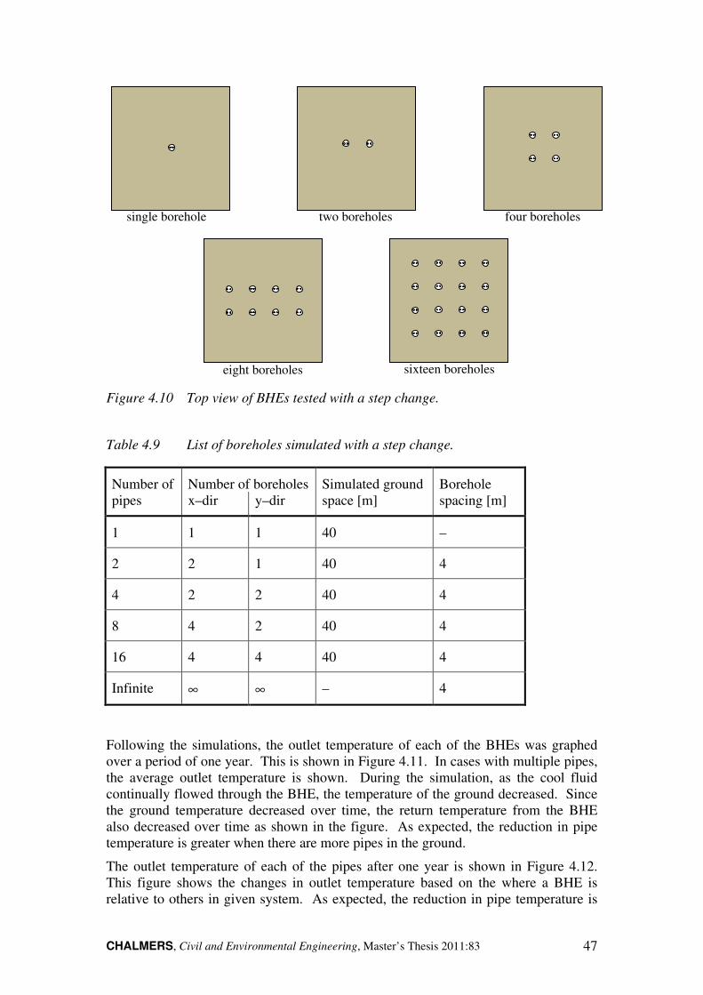
CHALMERS, Civil and Environmental Engineering, Master’s Thesis 2011:83 47
Figure 4.10 Top view of BHEs tested with a step change.
Table 4.9 List of boreholes simulated with a step change.
Number of Number of boreholes Simulated ground Borehole
pipes x–dir y–dir space [m] spacing [m]
1 1 1 40 –
2 2 1 40 4
4 2 2 40 4
8 4 2 40 4
16 4 4 40 4
Infinite ∞ ∞
– 4
Following the simulations, the outlet temperature of each of the BHEs was graphed
over a period of one year. This is shown in Figure 4.11. In cases with multiple pipes,
the average outlet temperature is shown. During the simulation, as the cool fluid
continually flowed through the BHE, the temperature of the ground decreased. Since
the ground temperature decreased over time, the return temperature from the BHE
also decreased over time as shown in the figure. As expected, the reduction in pipe
temperature is greater when there are more pipes in the ground.
The outlet temperature of each of the pipes after one year is shown in Figure 4.12.
This figure shows the changes in outlet temperature based on the where a BHE is
relative to others in given system. As expected, the reduction in pipe temperature is
single borehole two boreholes four boreholes
eight boreholes sixteen boreholes

CHALMERS, Civil and Environmental Engineering, Master’s Thesis 2011:83 48
greater when a BHE is in the core of a system and surrounded by other pipes. The
temperature reduction is the greatest for corner BHE.
Figure 4.11 Outlet temperature of a BHE in response to a step change in inlet
temperature.
Figure 4.12 Outlet temperature after one year of BHEs in response to a step
change in inlet temperature.
3.9
4
4.1
4.2
4.3
4.4
4.5
4.6
4.7
4.8
0 50 100 150 200 250 300 350
Tem
per
atu
re [
°C]
Time[days]
1 Borehole
2 Boreholes
4 Boreholes
8 Boreholes
16 Boreholes
Infinte Number
3.6
3.8
4
4.2
4.4
4.6
4.8
5
0 4 8 12 16 20
Tem
per
atu
re [
ºC]
Number of Pipes
Corner
Edge
Core
Infinite
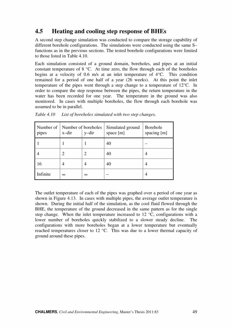
CHALMERS, Civil and Environmental Engineering, Master’s Thesis 2011:83 49
4.5 Heating and cooling step response of BHEs
A second step change simulation was conducted to compare the storage capability of
different borehole configurations. The simulations were conducted using the same S–
functions as in the previous sections. The tested borehole configurations were limited
to those listed in Table 4.10.
Each simulation consisted of a ground domain, boreholes, and pipes at an initial
constant temperature of 8 °C. At time zero, the flow through each of the boreholes
begins at a velocity of 0.6 m/s at an inlet temperature of 4°C. This condition
remained for a period of one half of a year (26 weeks). At this point the inlet
temperature of the pipes went through a step change to a temperature of 12°C. In
order to compare the step response between the pipes, the return temperature in the
water has been recorded for one year. The temperature in the ground was also
monitored. In cases with multiple boreholes, the flow through each borehole was
assumed to be in parallel.
Table 4.10 List of boreholes simulated with two step changes.
Number of Number of boreholes Simulated ground Borehole
pipes x–dir y–dir space [m] spacing [m]
1 1 1 40 –
4 2 2 40 4
16 4 4 40 4
Infinite ∞ ∞
– 4
The outlet temperature of each of the pipes was graphed over a period of one year as
shown in Figure 4.13. In cases with multiple pipes, the average outlet temperature is
shown. During the initial half of the simulation, as the cool fluid flowed through the
BHE, the temperature of the ground decreased in the same pattern as for the single
step change. When the inlet temperature increased to 12 °C, configurations with a
lower number of boreholes quickly stabilized to a slower steady decline. The
configurations with more boreholes began at a lower temperature but eventually
reached temperatures closer to 12 °C. This was due to a lower thermal capacity of
ground around these pipes.

CHALMERS, Civil and Environmental Engineering, Master’s Thesis 2011:83 50
Figure 4.13 Outlet temperature after one year of BHEs in response to a step
change in inlet temperature.
4
5
6
7
8
9
10
11
12
0 50 100 150 200 250 300 350
Tem
per
atu
re [
°C]
Time[days]
Inlet
1 Borehole
4 Boreholes
16 Boreholes
Infinite
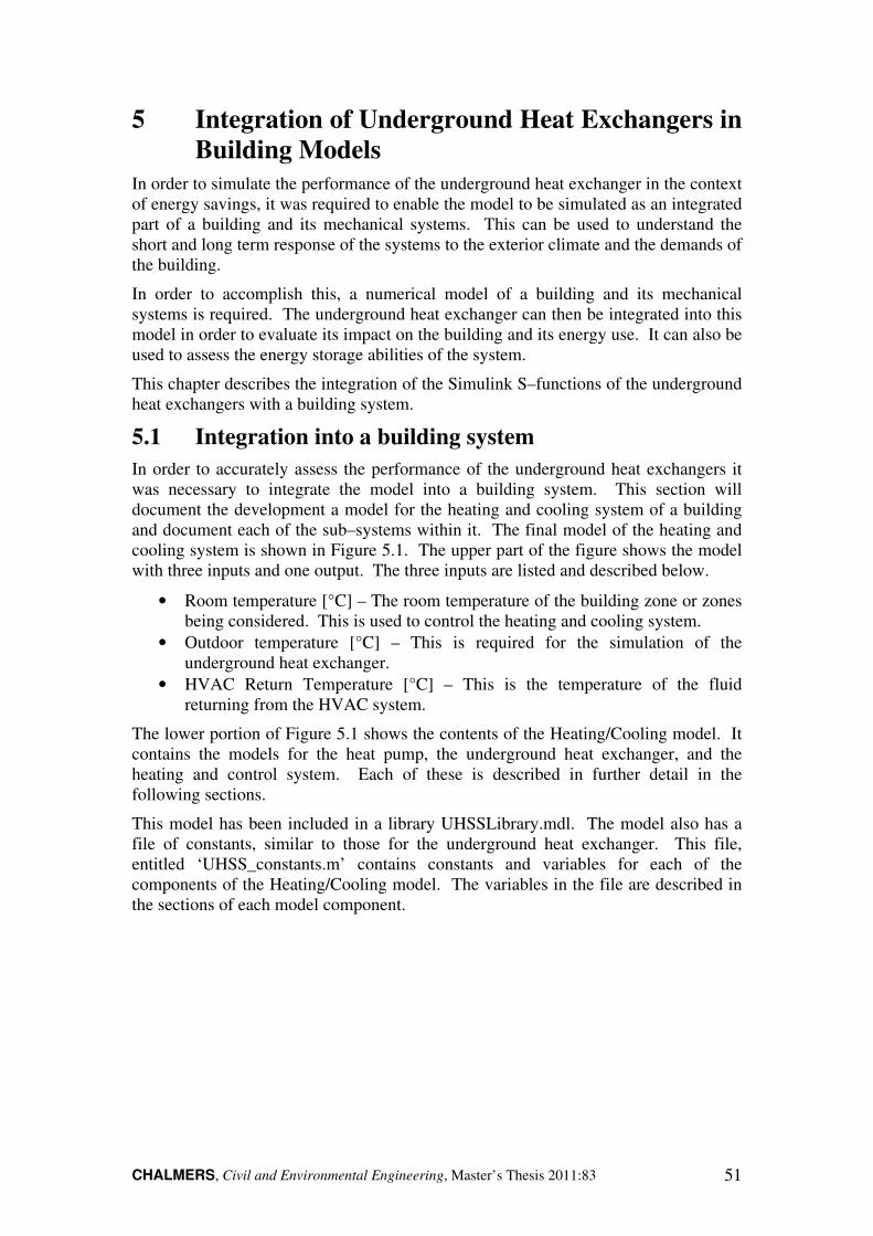
CHALMERS, Civil and Environmental Engineering, Master’s Thesis 2011:83 51
5 Integration of Underground Heat Exchangers in
Building Models
In order to simulate the performance of the underground heat exchanger in the context
of energy savings, it was required to enable the model to be simulated as an integrated
part of a building and its mechanical systems. This can be used to understand the
short and long term response of the systems to the exterior climate and the demands of
the building.
In order to accomplish this, a numerical model of a building and its mechanical
systems is required. The underground heat exchanger can then be integrated into this
model in order to evaluate its impact on the building and its energy use. It can also be
used to assess the energy storage abilities of the system.
This chapter describes the integration of the Simulink S–functions of the underground
heat exchangers with a building system.
5.1 Integration into a building system
In order to accurately assess the performance of the underground heat exchangers it
was necessary to integrate the model into a building system. This section will
document the development a model for the heating and cooling system of a building
and document each of the sub–systems within it. The final model of the heating and
cooling system is shown in Figure 5.1. The upper part of the figure shows the model
with three inputs and one output. The three inputs are listed and described below.
• Room temperature [°C] – The room temperature of the building zone or zones
being considered. This is used to control the heating and cooling system.
• Outdoor temperature [°C] – This is required for the simulation of the
underground heat exchanger.
• HVAC Return Temperature [°C] – This is the temperature of the fluid
returning from the HVAC system.
The lower portion of Figure 5.1 shows the contents of the Heating/Cooling model. It
contains the models for the heat pump, the underground heat exchanger, and the
heating and control system. Each of these is described in further detail in the
following sections.
This model has been included in a library UHSSLibrary.mdl. The model also has a
file of constants, similar to those for the underground heat exchanger. This file,
entitled ‘UHSS_constants.m’ contains constants and variables for each of the
components of the Heating/Cooling model. The variables in the file are described in
the sections of each model component.

CHALMERS, Civil and Environmental Engineering, Master’s Thesis 2011:83 52
Figure 5.1 Model of the heating and cooling system.
5.1.1 Model of the heat exchangers
The model of the heat exchangers contains both the model for the underground heat
exchanger along with a second heat exchanger between the heat pump and the
underground heat exchanger. This model is shown in Figure 5.3.
Scope
18
Room Temperature [°C]
10
Outdoor Temperature [°C]
Heating/Cooling
40
HVAC Return [°C]
HVAC Supply
1
Tout
TinHP
Power
Toutdoor
Tout
UHSS
HeatPumpOutput
RoomT [oC]
Power E [W]
Operateion Mode
Heat Cool Control
T UHSS_return [oC]
F UHSS_return [kg/s]
T HVAC_return [oC]
F HVAC_in [kg/s]
Ewp_max [W]
OpType
T UHSS_supply [oC]
T HVAC_supply [oC]
COP
Ewp [W]
HP Model (H+C)3
HVAC.flowrate
Fcond3
Treturn [oC]
2
Toutdoor
1
RoomT [oC]
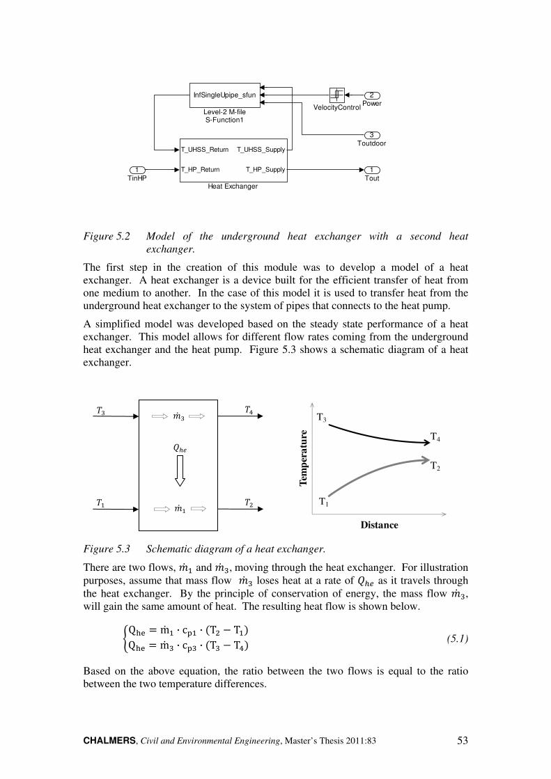
CHALMERS, Civil and Environmental Engineering, Master’s Thesis 2011:83 53
Figure 5.2 Model of the underground heat exchanger with a second heat
exchanger.
The first step in the creation of this module was to develop a model of a heat
exchanger. A heat exchanger is a device built for the efficient transfer of heat from
one medium to another. In the case of this model it is used to transfer heat from the
underground heat exchanger to the system of pipes that connects to the heat pump.
A simplified model was developed based on the steady state performance of a heat
exchanger. This model allows for different flow rates coming from the underground
heat exchanger and the heat pump. Figure 5.3 shows a schematic diagram of a heat
exchanger.
Figure 5.3 Schematic diagram of a heat exchanger.
There are two flows, {� Z and {� �, moving through the heat exchanger. For illustration
purposes, assume that mass flow {� � loses heat at a rate of 2�� as it travels through
the heat exchanger. By the principle of conservation of energy, the mass flow {� �,
will gain the same amount of heat. The resulting heat flow is shown below.
�Q�� ) m� Z · cMZ · 0TX * TZ1Q�� ) m� � · cM� · 0T� * Tx1 (5.1)
Based on the above equation, the ratio between the two flows is equal to the ratio
between the two temperature differences.
1
Tout
VelocityControl
InfSingleUpipe_sfun
Level-2 M-fileS-Function1
T_UHSS_Return
T_HP_Return
T_UHSS_Supply
T_HP_Supply
Heat Exchanger
3
Toutdoor
2
Power
1
TinHP
,� {� �
{� Z
,x
,Z ,X
2��
Tem
per
atu
re
Distance
T3
T4
T1
T2

CHALMERS, Civil and Environmental Engineering, Master’s Thesis 2011:83 54
m� �m� Z ) 0T� * Tx10TX * TZ1 (5.2)
The efficiency, η�, is defined as the ratio of the sum of the two temperature
differences divided by the total temperature difference as shown below.
η� ) 0T� * Tx1 7 0TX * TZ10T� * TZ1 (5.3)
Based on the results of these equations and definitions, the temperatures TX and Tx can
be calculated.
TX ) η� · 0T� * TZ14m� � · cM�m� Z · cMZ 7 15
· m� � · cM�m� Z · cMZ 7 ,Z (5.4)
Tx ) T� * η� · 0T� * TZ14m� � · cM�m� Z · cMZ 7 15
(5.5)
The completed model in Simulink is shown below in Figure 5.4.
Figure 5.4 Simulink model of a heat exchanger.
The user has control over two variables that control the performance of the heat
exchanger. These are listed in Table 5.1 and are included in the file
‘UHSS_constants.m’.
Table 5.1 List of variables in the model of a heat exchanger.
Input Variable Description Units
HE.efficiency Efficiency, η�, of the heat exchanger –
HE.flowratio Ratio of flow in the underground heat
exchanger to the flow in the heat pump
–
2
T_HP_Supply
1
T_UHSS_Supply
HE.efficiency
k
Subtract2
Subtract1
Subtract
Product
HE.flowratio
Flow RatioDivide1
Divide
u+1
Bias
2
T_HP_Return
1
T_UHSS_Return

CHALMERS, Civil and Environmental Engineering, Master’s Thesis 2011:83 55
5.1.2 Modelling of a heat pump
Heat pumps were modelled with a series of equations and the COMSOL models of
the underground heat exchangers were integrated with Simulink. The heat pump is
modelled with some simple differential equations as shown in A. W. M. van Schijndel
and de Wit (2003). The three equations used are shown below.
¡¢£¢¤COP ) k · 0.5 · Ty§h 7 0.5 · Ty¨©� 7 273.1500.5 · Ty§h 7 0.5 · Ty¨©�1 * 00.5 · T«§h 7 0.5 · T«¨©�1Cy dTy¨©�dt ) m� y§h · c · 0Ty§h * Ty¨©�1 7 COP · E�M
C« dT«¨©�dt ) m� «§h · c · 0T«§h * T«¨©�1 * 0COP * 11 · E�M (5.6)
The model was developed for a heat pump with a coefficient of performance, COP,
[–] as defined by the first equation in the set. In the ideal case the COP is equal to the
average temperature of the condenser (in Kelvin) divided by the temperature
difference between the compressor and the evaporator. To model more realistic
situation the efficiency, k, is implemented.
The second two equations model the performance of both the condenser and the
evaporator. In each case, the change in temperature of each reservoir is proportional
to the mass flow,m� through it; the electric power, Ehp, input, and the capacity, C, of
the system. The specific thermal capacity of the fluid is denoted by c. The subscript
c indicates the fluid at the condenser, v is the fluid at the evaporator, in is incoming,
and out is outgoing.
This model was implemented as an S–function and modifications to the model were
implemented to convert the heat pump into a reversible system to accommodate the
use of the heat pump for both heating and cooling.
The user has control over a number of variables that control the performance of the
heat pump. These are listed in Table 5.2 and are included in the file
‘UHSS_constants.m’.
Table 5.2 List of variables in the model of a heat pump.
Input Variable Description Units
HP.WPTC2 Heating – High Temperature Limit °C
HP.WPTC1 Heating – Low Temperature Limit °C
HP.WPTH2 Cooling – High Temperature Limit °C
HP.WPTH1 Cooling – Low Temperature Limit °C
HP.WPkw Efficiency of the heat pump –
HP.Evap_Cap Evaporator Capacity J/(kg*K)
HP.Comp_Cap Compressor Capacity J/(kg*K)

CHALMERS, Civil and Environmental Engineering, Master’s Thesis 2011:83 56
The temperature limits are used in the control of the operation of the heat pump. The
heat pump will turn off and resume operation based on the limits. For example the
shut down once the heating reservoir is above the high temperature limit and will then
resume operation once the temperature has fallen below the low temperature limit.
The other variables are used in the calculations shown in Equation (5.6).
The Simulink model of the heat pump is shown in Figure 5.5. The heat pump object
calls an S–function model of the heat pump. The OnOffControl object at the bottom
of the figure is used to shut off and resume operation of the heat pump based on the
temperature limits described above.
Figure 5.5 Simulink model of a heat pump.
4
Ewp [W]
3
COP
2
T HVAC_supply [oC]
1
T UHSS_supply [oC]
Product
T UHSS_supply [oC]
T HVAC_supply [oC]
opt
OnOf f 1
OnOf f 2
OnOffControl
T UHSS_return [oC]
F UHSS_return [kg/s]
T HVAC_return [oC]
F HVAC_in [kg/s]
E [W]
k
OpTy pe
Ev ap_Cap
Comp_Cap
UHSS_sup / HVAC_sup / COP
Heat Pump
HP.Evap_Cap
Evap_Cap
HP.WPkw
Constant-k
HP.Comp_Cap
Comp_Cap
6
OpType
5
Ewp_max [W]
4
F HVAC_in [kg/s]
3
T HVAC_return [oC]
2
F UHSS_return [kg/s]
1
T UHSS_return [oC]
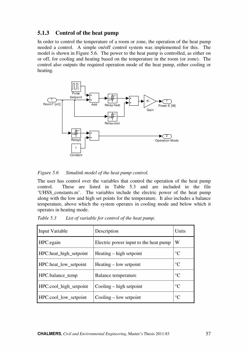
CHALMERS, Civil and Environmental Engineering, Master’s Thesis 2011:83 57
5.1.3 Control of the heat pump
In order to control the temperature of a room or zone, the operation of the heat pump
needed a control. A simple on/off control system was implemented for this. The
model is shown in Figure 5.6. The power to the heat pump is controlled, as either on
or off, for cooling and heating based on the temperature in the room (or zone). The
control also outputs the required operation mode of the heat pump, either cooling or
heating.
Figure 5.6 Simulink model of the heat pump control.
The user has control over the variables that control the operation of the heat pump
control. These are listed in Table 5.3 and are included in the file
‘UHSS_constants.m’. The variables include the electric power of the heat pump
along with the low and high set points for the temperature. It also includes a balance
temperature, above which the system operates in cooling mode and below which it
operates in heating mode.
Table 5.3 List of variable for control of the heat pump.
Input Variable Description Units
HPC.egain Electric power input to the heat pump W
HPC.heat_high_setpoint Heating – high setpoint °C
HPC.heat_low_setpoint Heating – low setpoint °C
HPC.balance_temp Balance temperature °C
HPC.cool_high_setpoint Cooling – high setpoint °C
HPC.cool_low_setpoint Cooling – low setpoint °C
2
Operation Mode
1
Power E [W]
Relay2
Relay-heat
Relay-cool
Pulse
Setpoint
-K-
Gain
1
Constant
Add
1
RoomT [oC]

CHALMERS, Civil and Environmental Engineering, Master’s Thesis 2011:83 58
6 Performance of Underground Heat Exchangers
6.1 Response of a simple building model
In order to examine the integrated performance of BHEs, a number of simulations
were conducted using a simple building model. In order to get a relatively
straightforward comparison, a simple building model was used.
6.1.1 The ISE model of a building
ISE (Indoor temperature Simulink Engineering tool) is a simplified modelling tool for
the simulation of the temperature response of a single zoned building (A. W. M. van
Schijndel, 2003). It is used in Simulink with user–friendly graphical interface. ISE
was designed to be used in the following situations:
1. A simple evaluation of the indoor temperature performance of a building
2. A simple estimate of both the heating a cooling potential and capacity
3. Allow for the evaluation and design of building systems and controls
The interface of the model in Simulink is shown in Figure 6.1.
The ISE model implements a model of a single building zone using the State Space
equation in Simulink to simulate the performance of a building. The Simulink model
is shown in Figure 6.2. The model treats the building as a single zone with a limited
number of inputs. The model accounts for heat conduction and radiation through the
wall and windows of the building and has additional inputs for internal heat gains and
the output of the heating and cooling system. The model then computes the internal
temperature in the zone. It also implements a temperature controller for regulating the
heating and cooling output.
Figure 6.1 ISE (Indoor temperature Simulink Engineering tool).

CHALMERS, Civil and Environmental Engineering, Master’s Thesis 2011:83 59
Figure 6.2 ISE Building ZONE model.
The ISE building model allows the user to input a number of parameters describing
the building. This includes the volume of the building along with characteristics of
the floor, walls, and windows. The parameters that can be input by the user are shown
in Figure 6.3.
Figure 6.3 Parameters of the ISE Building ZONE model.
1
Output
x' = Ax+Bu
y = Cx+Du
State-Space
Scope
1
Input

CHALMERS, Civil and Environmental Engineering, Master’s Thesis 2011:83 60
In order to include the performance of the underground heat exchangers it was
necessary to integrate these models into the ISE model. The original model’s heating
and cooling system simply consisted of a proportional system controlled by the
temperature difference between the indoor temperature and the desired temperature
set point. The heat flow into the building zone was computed in this model.
The model of the heating and cooling system with an integrated underground heat
exchanger that had been developed previously and shown in Figure 5.1 required
modifications in order to be linked into the ISE model heating/cooling module. The
building model in the ISE model requires an input of the heat flow, Q heating/cooling
(W). This flow is the amount of heating or cooling determined by the control system
required to heat or cool the building. Due to this, a module was developed to simulate
a heating and cooling system. The model of the integrated system is shown in Figure
6.4.
Figure 6.4 Model of the heating/cooling system with an integrated underground
heat exchanger.
The model developed to simulate a heating and cooling system is shown in Figure 6.5.
This model determines the quantity of heating or cooling, Qout, required by the
building zone. The output of the heating and cooling system is simply based on the
average temperature of the fluid flowing through the system, the temperature of the
room, and a heat transfer coefficient, K [W/K].
Q¨©� ) K · 4T�,§h 7 T�,¨©�2 * T°¨¨±5 (6.1)
To model the transient performance of the system a lumped model was developed.
The model consisted of the heating and cooling system with a capacity of C�«²y. The
change in energy of the system is simply the difference between the output of the
system, the input to the system, and the change in energy. The resulting equation is
shown below.
1
Qout
TinHP
Power
Toutdoor
Tout
UHSS
T HVAC Supply [oC]
T Room [oC]
T HVAC Return [oC]
Qout [W]
Simulate HVAC
RoomT [oC]
Power E [W]
Operation Mode
Heat Cool Control
T UHSS_return [oC]
F UHSS_return [kg/s]
T HVAC_return [oC]
F HVAC_in [kg/s]
Ewp_max [W]
OpTy pe
T UHSS_supply [oC]
T HVAC_supply [oC]
COP
Ewp [W]
HP Model (H+C)2
.34
Fcond
2
Toutdoor
1
RoomT [oC]

CHALMERS, Civil and Environmental Engineering, Master’s Thesis 2011:83 61
C�«²y dT�,¨©�dt ) m� �«²y · cM · �T�,§h * T�,¨©�� * K · 4T�,§h 7 T�,¨©�2 * T°¨¨±5 (6.2)
The temperature output of the heating system is solved for in the equation. From this
result, the heat output of the system is determined from Equation (6.1). The resulting
model, developed in Simulink is shown in Figure 6.5.
Figure 6.5 Model of the heating/cooling system.
6.1.2 Simulation details
The simulations, using the ISE model with an integrated geothermal heat pump were
executed for two locations. The locations chosen were De Bilt, The Netherlands and
Gothenburg, Sweden. Weather data was available for both of these locations. Three
year simulations were conducted. The buildings were simulated with the same
parameters relating to the size and other characteristics of the building. The
parameters used for the simulations are shown in Table 6.1
Table 6.1 Building parameters for the building simulations
Description Value Units
Building Volume 500 m3
Ventilation Rate 1 ach
Facade Surface Area 242 m2
Facade R Value 2.5 m2K/W
Internal Wall Area 100 m2
Window Surface Area 16 m2
Window R Value 0.33 m2K/W
The operation of the heat pump was controlled using the system detailed in Section
5.1.3. The temperature setting for the heat pump are shown below in Table 6.2
2
Qout [W]
1
T HVAC Return [oC]
f(u)
total heat
f(u)
derivative
1
s
Integrator
2
T Room [oC]
1
T HVAC Supply [oC]

CHALMERS, Civil and Environmental Engineering, Master’s Thesis 2011:83 62
Table 6.2 Temperature control settings for the heat pump.
Temperatures [°C]
Balance
Heating Cooling
Low High Low High
22.5 20 21.5 24.5 26
In the ISE model, thirty years of weather data for De Bilt was included from the year
1971 to 2000. The simulations were conducted over the years from 1973 to 1975.
This was done, since the average outdoor temperature in each of these years was near
the average for the entire time period. The outdoor temperature for the selected time
period is shown in Figure 6.6. Three full years of weather data were available for
Gothenburg from 2004 to 2006. The outdoor temperature for this period is shown in
Figure 6.7.
BHEs were used in each of the systems. The model InfSingleUpipe_sfun.m was used
for the simulations. The spacing between the pipes simulated at a four and six metre
spacing to get an indications on the effects of pipe spacing. A full list of the
parameters used for the heat exchanger is listed in Table 6.3 and Table 6.4.
Internal heat loads were also included in the buildings models. This was done to
ensure there was a cooling load in the building at certain parts of the year. The
amounts are listed in Table 6.5. The relatively high loads for the Gothenburg
simulations were chosen to simulate a building with considerable cooling loads in
order to assess energy storage capabilities.

CHALMERS, Civil and Environmental Engineering, Master’s Thesis 2011:83 63
Table 6.3 List of static parameters, mesh variables, and an output variable in the
BHE constant files used for the building simulations.
Input Variable Value Units
Static parameters
U_pipe.pipelength 200 m
U_pipe.pipedepth 2 m
U_pipe.soilspace 20 m
U_pipe.boreholediameter 0.13 m
U_pipe.relativepipelocation 0.8 –
U_pipe. TsoilinitialdegC 9.8 °C
U_pipe. Boreholespace1
4 and 6 M
Mesh Variables
U_pipe.mesh_geom1_hauto 8 –
U_pipe.mesh_geom2_hmax 4 M
Output Variable
U_pipe.outputdetails 1 –
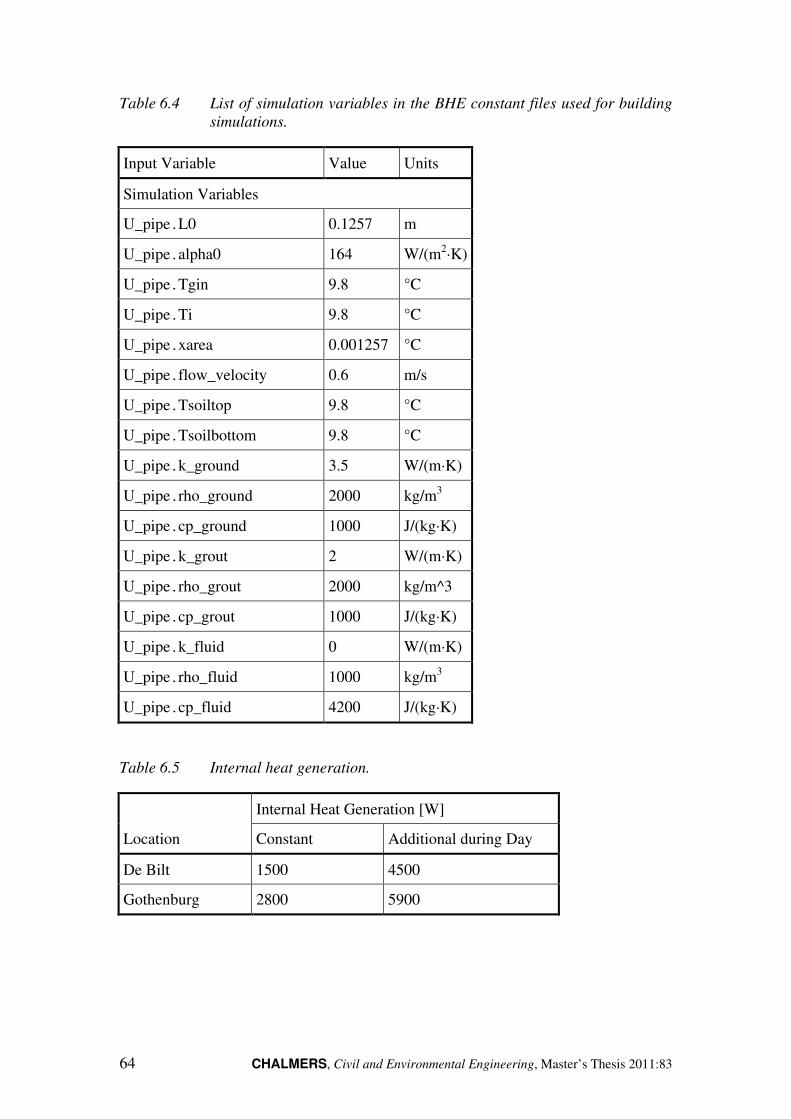
CHALMERS, Civil and Environmental Engineering, Master’s Thesis 2011:83 64
Table 6.4 List of simulation variables in the BHE constant files used for building
simulations.
Input Variable Value Units
Simulation Variables
U_pipe.L0 0.1257 m
U_pipe.alpha0 164 W/(m2·K)
U_pipe.Tgin 9.8 °C
U_pipe.Ti 9.8 °C
U_pipe.xarea 0.001257 °C
U_pipe.flow_velocity 0.6 m/s
U_pipe.Tsoiltop 9.8 °C
U_pipe.Tsoilbottom 9.8 °C
U_pipe.k_ground 3.5 W/(m·K)
U_pipe.rho_ground 2000 kg/m3
U_pipe.cp_ground 1000 J/(kg·K)
U_pipe.k_grout 2 W/(m·K)
U_pipe.rho_grout 2000 kg/m^3
U_pipe.cp_grout 1000 J/(kg·K)
U_pipe.k_fluid 0 W/(m·K)
U_pipe.rho_fluid 1000 kg/m3
U_pipe.cp_fluid 4200 J/(kg·K)
Table 6.5 Internal heat generation.
Location
Internal Heat Generation [W]
Constant Additional during Day
De Bilt 1500 4500
Gothenburg 2800 5900

CHALMERS, Civil and Environmental Engineering, Master’s Thesis 2011:83 65
Figure 6.6 Outdoor temperature in De Bilt, Netherlands (1973 to 1975).
Figure 6.7 Outdoor temperature in Gothenburg, Sweden (2004 to 2006).
0 200 400 600 800 1000 1200-15
-10
-5
0
5
10
15
20
25
30
35
Time [days]
Tem
pera
ture
[°C
]
0 200 400 600 800 1000 1200-15
-10
-5
0
5
10
15
20
25
30
35
Time [days]�
Tem
pera
ture
[°C
]

CHALMERS, Civil and Environmental Engineering, Master’s Thesis 2011:83 66
6.1.3 De Bilt results
The overall performance of the system was examined by calculating the energy use
and output of the buildings over the length of the simulation. Figure 6.8 and Figure
6.9 show the cumulative energy supplied to the building and electrical energy used by
the building respectively. The cumulative energy used after three years is tabulated
and shown in Table 6.6.
Figure 6.8 Cumulative absolute energy supplied to the building zone for the De
Bilt simulations.
Figure 6.9 Cumulative absolute energy supplied as electricity to the heat pump for
the De Bilt simulations.
0
5
10
15
20
25
30
35
40
0 200 400 600 800 1000 1200
Cu
mu
lati
ve
En
erg
y [
MW
h]
Time [days]
4 m spacing
6 m Spacing
0
1
2
3
4
5
6
7
8
0 200 400 600 800 1000 1200
Cu
mu
lati
ve
En
erg
y [
MW
h]
Time [days]
4 m Spacing
6 m Spacing

CHALMERS, Civil and Environmental Engineering, Master’s Thesis 2011:83 67
Table 6.6 Cumulative energy use in De Bilt Simulations
Borehole
spacing [m] Year
Energy [MWh]
COP Heating Cooling Cumulative Use HP Electrical
4 m
1 10.17 2.50 12.68 2.74 4.63
2 7.53 1.44 8.97 2.01 4.46
3 8.82 2.90 11.72 2.58 4.54
Total 26.53 6.84 33.37 7.33 4.55
6 m
1 10.17 2.50 12.67 2.70 4.69
2 7.54 1.43 8.97 1.91 4.70
3 8.82 2.91 11.73 2.54 4.61
Total 26.53 6.84 33.37 7.16 4.66
The temperature in the ground was also determined during the simulations. The
ground temperature at a depth midway along the borehole and two meters away are
compared in Figure 6.10.
Figure 6.10 Ground temperature at a distance of 2 m from the borehole for the De
Bilt Simulations.
8.6
8.8
9
9.2
9.4
9.6
9.8
10
0 200 400 600 800 1000 1200
Te
mp
era
ture
[°C
]
Time [days]
4 m spacing
6 m Spacing

CHALMERS, Civil and Environmental Engineering, Master’s Thesis 2011:83 68
Note that in the De Bilt simulations there was a cooling load, but it was significantly
lower than the heating load. This is demonstrated by the fact that the temperature in
the ground continued to decline over the length of the simulation. The results also
show a somewhat lower electrical energy use with greater pipe spacing.
6.1.4 Gothenburg results
The overall performance of the system was examined by calculating the energy use
and output of the buildings over the length of the simulation. Figure 6.11 and Figure
6.12 show the cumulative energy supplied to the building and electrical energy used
by the building respectively. The cumulative energy used after three years is
tabulated and shown in Table 6.7
Figure 6.11 Cumulative absolute energy supplied to the building zone for the
Gothenburg simulations.
0
5
10
15
20
25
30
0 200 400 600 800 1000 1200
Cu
mu
lati
ve
En
erg
y [
MW
h]
Time [days]
4 m spacing
6 m Spacing

CHALMERS, Civil and Environmental Engineering, Master’s Thesis 2011:83 69
Figure 6.12 Cumulative absolute energy supplied as electricity to the heat pump for
the Gothenburg simulations.
Table 6.7 Cumulative energy use in Gothenburg simulations.
Borehole
spacing [m] Year
Energy [MWh]
COP Heating Cooling Cumulative Use HP Electrical
4 m
1 2.82 6.49 9.31 1.88 4.95
2 2.15 6.72 8.87 1.81 4.91
3 0.44 5.08 5.52 1.02 5.41
Total 5.41 18.29 23.70 4.71 5.04
6 m
1 2.63 6.51 9.15 1.81 5.05
2 2.03 6.74 8.77 1.72 5.10
3 0.36 5.10 5.46 0.99 5.52
Total 5.02 18.36 23.37 4.52 5.17
The temperature in the ground was also determined during the simulations. The
ground temperature at a depth midway along the borehole and two meters away are
compared in Figure 6.13.
0
1
2
3
4
5
6
0 200 400 600 800 1000 1200
Cu
mu
lati
ve
En
erg
y [
MW
h]
Time [days]
4 m spacing
6 m spacing

CHALMERS, Civil and Environmental Engineering, Master’s Thesis 2011:83 70
Figure 6.13 Ground temperature at a distance of 2 m from the borehole for the
Gothenburg simulations.
In the Gothenburg simulations there was a higher cooling load than a heating load.
As a result, the trend in the temperature in the ground rises. There is, however, a
periodic fluctuation in the temperature as a result of heating and cooling. The results
also show a somewhat lower electrical energy use with higher pipe spacing.
6.1.5 Discussion
The results of the simulations give some preliminary results on the performance of
BHEs and their use in energy storage. The results from Gothenburg, particularly,
show the fluctuations in the temperature of the ground with underground heat storage.
There is a rise in the temperature of the ground during the cooling season and the
lowering of temperatures during the heating season can be observed. When designing
a system, a balance between the heat removed and the heat stored needs to be
maintained.
There also was a small decrease in the total energy use of the heat pump when the
pipe spacing was increased from four to six meters for both of the simulations. This
could be due, in heating for example, to lower ground temperatures around the
underground heat exchanger which could lead to lower temperature differences
between the inlet and outlet temperatures of the heat exchanger. This would result in
a lower heat output requiring longer operation of the heat pump and greater energy
use.
9.6
9.7
9.8
9.9
10
10.1
10.2
10.3
10.4
0 200 400 600 800 1000 1200
Te
mp
era
ture
[°C
]
Time [days]
4 m spacing
6 m Spacing

CHALMERS, Civil and Environmental Engineering, Master’s Thesis 2011:83 71
7 Case Study of an Existing Building: Anatomy
House
7.1 Development of a lumped thermal model
In order to simulate an existing building a simplified lumped thermal capacity model
was used to accomplish this. A lumped model is based on the assumption that the
spatial variation of temperature in a body is constant. That is, the temperature
variation across the body in space is negligible. The temperature in that body varies
with time depending on its thermal capacity and the heat flows into and out of the
body (Bejan and Kraus, 2003). For example, consider a body with a volume, V,
surface area, A´, density, ρ, and specific heat, cM, at an initial temperature of Ti. After
time t=0, there is conduction that occurs from an external temperature, T�µ�0t1, through a material with a conductance, U. Using the lumped model, the temperature
of the body, T, is determined with the differential equation of the process shown
below.
ρ · V · cM · dTdt ) *U · A´ · 0T * T�µ�0t11 (7.1)
With the initial condition:
T0t ) 01 ) T§ (7.2)
This example only shows the conduction into the body. To simulate a building all of
the significant heat flows are considered, such as solar radiation, conduction, wind
convection, internal heat gains, ventilation, and air leakage. The building can also be
divided into multiple bodies with thermal flows between them. The differential
equation for the lumped model of a body with only conduction into that body can be
solved using Simulink. The model for this is shown in Figure 7.1.
Figure 7.1 A simple lumped model of a building in Simulink with heat flow into the
body through conduction.
Subtract
Product
1/s
Integrator
Text
External TDivide
U
Conductance
C
Capacity
A
Area
Text(t)-T
UA(Text-T)
dT(t)/dtT(t)

CHALMERS, Civil and Environmental Engineering, Master’s Thesis 2011:83 72
The solution to Equation (7.1) can be solved for as the equation shown below when
assuming a constant exterior temperature, T�µ�. T0t1 ) T�µ� 7 0T§ * T�µ�1 · eH�/�¸ (7.3)
Where the time constant, ty is:
ty ) U · A´C (7.4)
The lumped capacity of the building, C, is found with the equation below:
C ) ρ · V · cM (7.5)
Using a simple numerical example, the solution to the differential equation was
compared to the Simulink model results for the temperature of the body. The results,
shown in Figure 7.2, show that Simulink calculates a solution that is identical to the
analytical solution.
Figure 7.2 Comparison of simple lumped model in Simulink with the analytical
solution of the equation.
A lumped model for a whole building can also be developed. For a simple building
the interior of the building can be modelled as one body. The temperature in the
interior of the building is assumed to be constant. There are also additional thermal
flows into and out of the building that need to be considered. These flows include
conduction through the walls and windows, air convection at surfaces, long and short
wave radiation, indoor heating systems, internal heat gains, ventilation, air
conditioning, and air leakage.
0
2
4
6
8
10
12
14
16
18
20
0 20000 40000 60000 80000 100000 120000 140000 160000
Te
mp
er
atu
re
[°
C]
Time[s]
Analytical
Simulink
CHALMERS, Civil and Environmental Engineering, Master’s Thesis 2011:83 73
In developing more complex models of building, multiple lumped bodies can be
modelled together in one simulation. For example a building could be divided into
two zones if there are two floors in the building. The model must then consider any
flows between the zones. The performance of different flows can also be modelled in
detail using Simulink. The thermal flows provided by a heating system, for example,
can be modelled to include proportional control and delayed thermal outflows.
7.2 Anatomy House (Anatomi Hus) at Salgrenska
Hospital in Gothenburg
In order to evaluate the underground heat exchanger and its integration into buildings,
a case study of an existing building was conducted. This case study investigated the
performance of the Anatomy House, an office building located in Göteborg, Sweden.
It is located near the Sahlgrenska University Hospital. Figure 7.3 shows an image of
the building and its surroundings.
The building was originally constructed in the 1960s as an anatomy laboratory, thus
the name Anatomy House. The building was later renovated during which the
laboratories were removed and replaced with offices. The renovation of the building
included the installation of a new ventilation and air conditioning system.
The new ventilation system was a Variable Air Volume (VAV) system. An air
conditioning plant was installed in the attic as part of the ventilation system. The
purpose of the air conditioning system is to maintain a supply air temperature to the
offices of 15 °C during working hours. The ventilation rates to the offices can be
adjusted based on the occupancy and when additional cooling is required.
This section presents the model developed in Simulink to model the Anatomy House.

CHALMERS, Civil and Environmental Engineering, Master’s Thesis 2011:83 74
Figure 7.3 Image and location of the Anatomy House in Göteborg (Microsoft,
2010).
7.2.1 Building characteristics
A lumped model of the building was developed to consider the main heat sources,
heat sinks, and components with a significant heat capacity. As a first step, a model
was developed for the fourth floor of the building. This model considered heat
conduction through the walls and windows, thermal radiation through the windows,
internal heat generation, ventilation and air leakage, and supplementary heating. The
floor was divided into two zones while accounting for cross–ventilation between
them. This section describes the assumptions and calculations that have been used to
model the Anatomy House. The assumptions and building characteristics are based
on a previous study (Sasic Kalagasidis, 2009). In this study complex simulations
were conducted of the Anatomy house using the building simulation program HAM–
Tools (Sasic Kalagasidis, 2004).
The response of each of the zones to thermal loads has been calculated using a lumped
thermal capacity of each zone. Typically, the thermal capacity of the building
envelope that contributes to the lumped capacity of the building interior is considered
to be only the thermal mass located on the interior side of the insulation within the
building envelope. The modeling of the Anatomy House was more challenging
because of the lack of insulation. The wall sections in the building consist of a solid
70 cm brick wall. To determine the thickness of the wall that contributed to the
lumped capacity, the penetration depth, 3�, of the wall was calculated using Equation

CHALMERS, Civil and Environmental Engineering, Master’s Thesis 2011:83 75
(7.6) with a time period, ��, of one day. This time period was used to model the daily
fluctuation in the indoor environment.
3� ) ¹q · ��V (7.6)
In addition to the brick wall double pane windows are part of the building envelope.
The thermal properties of the building envelope are shown in Table 7.1.
Table 7.1 Thermal properties of the building envelope.
Thermal
Conductivity Density
Heat
Capacity Emissivity Absorptivity
[W/m·K] [kg/m3] [J/kg·K] [–] [–]
Brick 0.7 1800 800 0.9 0.4
Glass 1 2500 750 0.9 0.06
A lumped model was also used for determining the outer temperature of the wall
which was used to calculate the heat conduction into the building. The same
penetration depth was used as described above. The heat flows used in this lumped
model include the heat flow through the wall to the interior, heat transfer at the
surface including convection, and heat flow due to long and short wave radiation.
The solar radiation absorbed on the wall is calculated using:
�º�=o»,zo== ) qo¼º,F · ½¾�F»��¿,F0�1 7 ¾�FÀÀÁº�0�1 · ÃF (7.7)
The heat transfer at the surface was calculated using:
!� ) 5.82 7 3.96 · � � Ç 5 {/È (7.8)
!� ) 7.68 · �".ÉÊ 7 3.96 · � � Ë 5 {/È (7.9)
The heat conduction from the interior through the wall was then calculated using
Equation (7.10).
2zo== ) ÌÃzo== · 0,FG¿�»F�» * ,�Á¿�»1 (7.10)
The lumped model developed for each interior zone also included the conduction.
The other heat flows include internal heat sources, conduction and solar radiation
through the windows, supply air ventilation, air leakage, supply heat, and cross
ventilation between the zones.
The intensity of the internal heat gains was based on the data from.... They are listed
in Table 7.2. The internal gains during the working hours from 8:00 to 18:00 are
3890 W. During non–working hours the internal heat gains are assumed to be 500W.

CHALMERS, Civil and Environmental Engineering, Master’s Thesis 2011:83 76
Table 7.2 Intensity of internal heat gains
Gain Type Description Total Gain [W]
People There are 12.6 (60%) out of possible
21, each releasing 80 W. 1010
Computers and Printers 8 W/m2 of floor area or 100 W per
office 1310
Office Lighting 7 W/m2 of floor area with 12.6 out
of 21 offices in use at the same time 1150
Corridor Lighting 5 W/m2 of floor area 420
Total 3890
Heat gains through the windows consisted of solar radiation and conduction.
Radiation was calculated using:
2º�=0�1 ) q · Í · ½¾�F»��¿,F0�1 · ÎZ0!1 7 ¾�FÀÀÁº�0�1 · ÎX · ÃzFG��z (7.11)
The transmittance ÎZ, is a function of the angle of incidence. The solar transmittance
was calculated using the values shown below in Table 7.3.
Table 7.3 Solar transmittance, ÎZ, versus solar incidence angle.
Ï 0 10 20 30 40 50 60 70 80 90
ÐÑ 0.747 0.747 0.745 0.74 0.73 0.707 0.652 0.517 0.263 0
The VAV system provides ventilation and cooling when the air is warm to the offices.
The air exchange rate is controlled as shown in Figure 7.4. The minimum air
exchange rate of 0.7 ACH is provided at all times. If the temperature rises above 21
°C the exchange rate is increased to 1 ACH. A maximum supply of 3 ACH is
provided when the temperature is at 25 °C or above. The air supply rate, as described,
is enabled during normal working hours from 6:00 to 19:00. During evenings and on
weekends a supply rate of 0.4 ACH is maintained. A supply air temperature of 15 °C
was maintained.

CHALMERS, Civil and Environmental Engineering, Master’s Thesis 2011:83 77
Figure 7.4 Supply air flow rate as controlled by the indoor air temperature during
working hours.
The total air supply to each zone was calculated based on the assumption that all of
the air supply units were of the same size and provided the same ventilation rate. This
means that the total air supply to the floor was based on the number of vents as shown
in Equation (7.12). The total ventilation for the floor was 23.7 % of the total
ventilation.
2o,À=��» ) (�{Í%w r È�;;�� q'w �('�È ;%w r�w��q� (�{Í%w r È�;;�� �('�È · 2o,¿�¿o= (7.12)
The difference between the supply and exhaust flow rate was found to be
approximately 35%. The exhaust fan takes more air out than is introduced by the
supply fan resulting in an under–pressurization of the building. The air leakage, in the
calculations, was assumed to be 35% during working hours and zero during nights
and weekends.
There is no solid partition between the north and south zone of the building. During
normal conditions it is assumed that many doors are left ajar and there is a significant
amount of air movement between the zones. Based on this assumption an exchange
rate of 3 ACH of cross ventilation was simulated.
The cooling load on the zone and for the air conditioning system was determined
during the simulations. The cooling load in the air conditioning plant was calculated
by determining how much cooling was required to maintain a constant supply air
temperature. The design temperature, ,ºÁ��=Ò, was 13 °C.
2���=,��F= ) � 0 'r ,�Á¿ Ç ,ºÁ��=Ò$ · �� · 2o,¿�¿o=0�1 · ½,�Á¿0�1 * ,ºÁ��=Ò 'r ,�Á¿ Ë ,ºÁ��=Ò (7.13)

CHALMERS, Civil and Environmental Engineering, Master’s Thesis 2011:83 78
The effect of ventilation on the interior zones of the building was based on the
ventilation rate as described in Figure 7.4 and the temperature difference between the
interior temperature and the supply air temperature as described in Equation (7.14).
2Ó�G¿ ) $ · �� · 2o,¿�¿o=0�1 · ½,ºÁ��=Ò * ,Ô�G�0�1 (7.14)
The heating load was calculated based on the heat required to maintain an indoor air
temperature of 21 °C during working hours and 20 °C during nights and weekends.
7.2.2 Simulink model of the building
The model of the Anatomy House, developed in Simulink, divided the building into a
north zone and a south zone. The loads and temperatures are then simulated for each
zone with the cross ventilations between them. The final model of the building is
shown in Figure 7.5. The figure shows the subsystems for each of the north and south
zone, along with the air conditioning and heating systems for each.
Figure 7.5 Simulink model of the Anatomy House
The model of each of the entire interior zones, as shown in Figure 7.6, determines the
thermal loads from the exterior walls and inputs the results to the model of the interior
zone. In each of the wall subsystems an equivalent exterior temperature of the wall is
calculated along with the heat transfer through the windows. These values are then
output to the interior zone.
simoutsouthwall
To Workspace4
simoutsouth
To Workspace3
simoutnorthwall
To Workspace2
simoutnorth
To Workspace1
GBGweather_SMHI
text
From
TinCrossVent
Qheatcool
Tin
Qout
Qwallgains
GeomOut
EntireZone-South
TinCrossVent
Qheatcool
Tin
Qout
Qwallgains
GeomOut
EntireZone-North
Tout
Tin
Qtot
Qload
AirConditioning+Heat-south
Tout
Tin
Qtot
Qload
AirConditioning+Heat-north

CHALMERS, Civil and Environmental Engineering, Master’s Thesis 2011:83 79
Figure 7.6 Simulink model of entire zone of the Anatomy House
The equivalent exterior temperature of the wall was determined by modelling the
exterior portion of the wall as a lumped system. The subsystem model is shown in
Figure 7.7. The heat transfer into the section of the wall due to the exterior weather is
calculated in the ‘Outdoor surface weather conditions, walls and roof’ subsystem.
The heat transfer from the interior of the building is also calculated based on the
temperature difference between the interior temperature and the equivalent exterior
temperature. The resulting loads are divided by the lumped capacity of the system
and then integrated at each time step to find the equivalent wall temperature. The heat
transfer through the windows is also calculated in this subsystem.
4
GeomOut
3
Qwallgains
2
Qout
1
Tin
Textern
TinCrossVent
QwindowsRad
WallTout
Qheatcool
Tin
QOut
Zone
Scope1
Scope
ZoneInfo(zone_num).Orientations
ZoneInfo(zone_num).Tilts
ZoneInfo(zone_num).Areas
Geometry
text
From
Geometry
TWallInt
TwallExt
Qwindow
Qgains
AllExteriorWallWindows4
Geometry
TWallInt
TwallExt
Qwindow
Qgains
AllExteriorWallWindows3
Geometry
TWallInt
TwallExt
Qwindow
Qgains
AllExteriorWallWindows1
2
Qheatcool
1
TinCrossVent

CHALMERS, Civil and Environmental Engineering, Master’s Thesis 2011:83 80
Figure 7.7 Simulink subsystem of the lumped model of the exterior walls and
windows
The subsystem of the heating and air conditioning system for the building is shown in
Figure 7.8. Seperate systems are modelled for each zone. The output of the heating
system is a proportional control calculated from the temperature difference between
the interior of the zone and the temperature setpoint. The ventilation system is
modelled on the description shown in the previous section with a ventilation rate
shown in Figure 7.4. The subsystem output two different heat flows. Qout is the
amount of heat transfer directly into the building zone. Qload is the amount of energy
used to heat or cool the air in the ventilation system to the desired temperature.
3
Qgains
2
Qwindow
1
TwallExt
Surf aceWeather WindowFlux
WindowRadiation
GeomSurface w eather data
Weather on surface
Weather
Tsurf
Heat from exterior
Outdoor surface conditions
walls and roof1
s
Integrator-K-
Gain-UA
-K-
Gain-Area
Divide-C-
CapacityAdd1
Add
2
TWallInt
1
Geometry

CHALMERS, Civil and Environmental Engineering, Master’s Thesis 2011:83 81
Figure 7.8 Simulink subsystem of the heating and air conditioning model
The final lumped model calculations for the interior zone of the building are done in
the subsystem shown in Figure 7.9. This model considers all of the thermal loads that
have been described and computes the resulting interior temperature of the zone. The
model considers all of the passive loads along with the heating and cooling loads from
the mechanical systems.
2
Qload
1
Qtot
TSupply
Tsupply
Sum of
Elements
Subtract1
Subtract
Scope1
Saturation1Saturation
Pulse-Week1
Pulse-Week
Pulse-Day
Pulse
Generator
Product4
Product3 Product2Product1
Merge
Merge
PercentLeakage
Leakage
if { }Tout
Tsupply
Tin
Pulse
QheatIndoor
If Action
Heat Air
else { }Tout
Tsupply
Tin
Pulse
QCoolingIndoor
If Action
Cooling
u1
u2
if (u2<=u1)
else
If
-K-
Gain
TSetpoint(1)
Constant_Tsetpoint
-C-
Constant1
Add
2
Tin
1
Tout
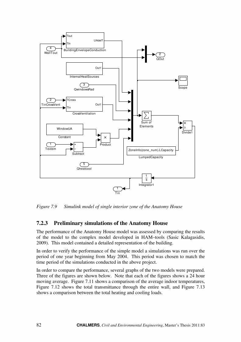
CHALMERS, Civil and Environmental Engineering, Master’s Thesis 2011:83 82
Figure 7.9 Simulink model of single interior zone of the Anatomy House
7.2.3 Preliminary simulations of the Anatomy House
The performance of the Anatomy House model was assessed by comparing the results
of the model to the complex model developed in HAM–tools (Sasic Kalagasidis,
2009). This model contained a detailed representation of the building.
In order to verify the performance of the simple model a simulations was run over the
period of one year beginning from May 2004. This period was chosen to match the
time period of the simulations conducted in the above project.
In order to compare the performance, several graphs of the two models were prepared.
Three of the figures are shown below. Note that each of the figures shows a 24 hour
moving average. Figure 7.11 shows a comparison of the average indoor temperatures,
Figure 7.12 shows the total transmittance through the entire wall, and Figure 7.13
shows a comparison between the total heating and cooling loads.
2
QOut
1
Tin
Sum of
Elements
Subtract
Scope
Product
ZoneInfo(zone_num).LCapacity
LumpedCapacity
Out1
InternalHeatSources
1
s
Integrator1
Divide1
TCross
TInOut1
CrossVentilation
WindowUA
Constant
Tout
TinUAdelT
BuildingEnvelopeConduction
5
Qheatcool
4
WallTout
3
QwindowsRad
2
TinCrossVent
1
Textern

CHALMERS, Civil and Environmental Engineering, Master’s Thesis 2011:83 83
Figure 7.10 Comparison of the 24 hour moving average of indoor temperatures in
the simplified and complex models of the Anatomy house
Figure 7.11 Comparison of a 24 hour moving average of the total wall transmission
in the simplified and complex models of the Anatomy house
19
20
21
22
23
24
25
26
27
28
0 50 100 150 200 250 300 350
Av
era
ge
Ind
oo
r Te
mp
era
ture
[°C
]
Time [days]
24 per. Mov. Avg. (Simplified)
24 per. Mov. Avg. (Complex)
-8
-7
-6
-5
-4
-3
-2
-1
0
1
2
0 50 100 150 200 250 300 350
Tota
l W
all
Tra
nsm
issi
on
[k
W]
Time [days]
24 per. Mov. Avg. (Simplified)
24 per. Mov. Avg. (Complex)

CHALMERS, Civil and Environmental Engineering, Master’s Thesis 2011:83 84
Figure 7.12 Comparison of a 24 hour moving average of the heating and cooling
rates in the simplified and complex models of the Anatomy house
The results from the figures do show similar trend in the performance of the building.
For example, both models show elevated temperatures in the building around day 100.
The simple model however, shows significantly higher temperatures than the complex
model. The simple model also shows higher heating loads during the period from
approximately day 200 to day 350. These observations could indicate that some of
the simplifications made in the model result in some errors in the calculations. It was
decided, however, to proceed with the integration of a heat pump model into the
simplified model, since the general trends in the performance of the two models were
similar.
7.2.4 Development of a model including ground coupled heat
pumps
In order to integrate the underground heat pumps into the model of the Anatomy
house, the models of the heating systems for each zone were combined into a single
model. The air conditioning and ventilation systems were kept as separate objects. In
this simulation only the primary heating system of the building was integrated with
the ground couple heat pump. The primary heating system is separate from the
cooling and air conditioning system and can be simply modified to integrate the
underground heat pump system. This was implemented to see the impacts of adding
the system to the building. The Simulink model of the building with the combined
system is shown in Figure 7.13.
-10
-5
0
5
10
15
20
0 50 100 150 200 250 300 350
Tota
l H
ea
tin
g a
nd
Co
oli
ng
[k
W]
Time [days]
24 per. Mov. Avg. (Complex)
24 per. Mov. Avg. (Simplified)

CHALMERS, Civil and Environmental Engineering, Master’s Thesis 2011:83 85
Figure 7.13 Simulink model of the Anatomy House modified to include a heating
and cooling system with integrated underground heat exchangers
The subsystem of the integrated heating and cooling system is shown in Figure 7.14.
It contains models for the heat pump, underground heat exchanger, the control system,
and the heating system. The model then outputs the total heat flows into each zone.
simoutsouthwall
To Workspace4
simoutsouth
To Workspace3
simoutnorthwall
To Workspace2
simoutnorth
To Workspace1
Heating
HVAC Integrated
GBGweather_SMHI
text
From
TinCrossVent
Qheatcool
Tin
Qout
Qwallgains
GeomOut
EntireZone-South
TinCrossVent
Qheatcool
Tin
Qout
Qwallgains
GeomOut
EntireZone-North
Tout
Tin
Qheat
Qtot
Qload
AirConditioning+Heat-south
Tout
Tin
Qheat
Qtot
Qload
AirConditioning+Heat-north

CHALMERS, Civil and Environmental Engineering, Master’s Thesis 2011:83 86
Figure 7.14 Simulink subsystem of the heating and air conditioning model
7.2.5 Simulation of the Anatomy House with BHEs
The model with the integrated BHEs was simulated over the same time period as the
previous simulations in order to determine their impact. The overall temperature
comparison is shown in Figure 7.15. As expected, the temperature trends compared
between the two simulations are quite similar. There are, however, some differences
that can be seen in the short term response. Figure 7.16 shows the temperature
response over a period of one week.
This figure shows the cyclic nature of the heat pump performance. Due to the slower
response and the fact that the heat pump turns off and on due to temperature limits the
interior temperature has a more cyclic response. In reality, the cycles shown in the
figure could be reduced, but there would most likely be more fluctuations than with
the direct heating simulated with the simple model. The simple model simulated
direct proportional heating into the interior zone of the building. In reality there
would be more fluctuations in this temperature as well, as there would be delays in the
response as well.
Table 7.4 shows the total amount of energy output by the heating system integrated
with the heat pump along with the total electrical energy used to power the heat pump.
The heat pump over the length of the simulation has an average COP of 4.8. This is
theoretically quite high, but does give an indication that a large amount of heat is
obtained from the ground with a significantly reduced input.
2
QoutS
1
QoutN
TinHP
Power
Toutdoor
Tout
UHSS1
(u(1)+u(2))/2
Mean
RoomT [oC]Power E [W]
Operation Mode
Heat Cool Control
T UHSS_return [oC]
F UHSS_return [kg/s]
T HVAC_return [oC]
F HVAC_in [kg/s]
Ewp_max [W]
OpTy pe
T UHSS_supply [oC]
T HVAC_supply [oC]
COP
Ewp [W]
HP Model (H+C)3
T HVAC Supply
T Room
RoomTs
T HVAC Return
QoutN
QoutS
FullHVACHeat
HVAC.flowrate
Fcond
3
Toutdoor
2
RoomTS[oC]
1
RoomTN [oC]

CHALMERS, Civil and Environmental Engineering, Master’s Thesis 2011:83 87
Table 7.4 Cumulative energy use for heating system
Energy [MWh]
COP Heating Output HP Electrical
29.2 6.1 4.8
Figure 7.15 Comparison of the average indoor temperatures in the simplified model
with and without an underground heat pump system over one year
19
20
21
22
23
24
25
26
27
28
0 50 100 150 200 250 300 350
Av
era
ge
Ind
oo
r Te
mp
era
ture
[°C
]
Time [days]
24 per. Mov. Avg. (With BHE)
24 per. Mov. Avg. (Simplified)

88
Figure
The temperature of the ground at the centre depth of the pipe at a distance t
from the pipe over the year of the simulations is shown in
since only heating was used, the temperature in the ground decreases over the year
once significant use of the heating system has begu
Figure
88
Figure
The temperature of the ground at the centre depth of the pipe at a distance t
from the pipe over the year of the simulations is shown in
since only heating was used, the temperature in the ground decreases over the year
once significant use of the heating system has begu
Figure
Av
era
ge
Ind
oo
r Te
mp
era
ture
[°C
]
Figure
The temperature of the ground at the centre depth of the pipe at a distance t
from the pipe over the year of the simulations is shown in
since only heating was used, the temperature in the ground decreases over the year
once significant use of the heating system has begu
Figure
19
19.5
20
20.5
21
21.5
22
22.5
23
23.5
24
Figure 7.
The temperature of the ground at the centre depth of the pipe at a distance t
from the pipe over the year of the simulations is shown in
since only heating was used, the temperature in the ground decreases over the year
once significant use of the heating system has begu
Figure 7.
19
19.5
20
20.5
21
21.5
22
22.5
23
23.5
24
250
.16
The temperature of the ground at the centre depth of the pipe at a distance t
from the pipe over the year of the simulations is shown in
since only heating was used, the temperature in the ground decreases over the year
once significant use of the heating system has begu
.17
250
Comparison of the average indoor temperatures in the simplified model
with and without
The temperature of the ground at the centre depth of the pipe at a distance t
from the pipe over the year of the simulations is shown in
since only heating was used, the temperature in the ground decreases over the year
once significant use of the heating system has begu
Ground temperature at a distance of 2
simulation of the
251
CHALMERS
Comparison of the average indoor temperatures in the simplified model
with and without
The temperature of the ground at the centre depth of the pipe at a distance t
from the pipe over the year of the simulations is shown in
since only heating was used, the temperature in the ground decreases over the year
once significant use of the heating system has begu
Ground temperature at a distance of 2
simulation of the
CHALMERS
Comparison of the average indoor temperatures in the simplified model
with and without an
The temperature of the ground at the centre depth of the pipe at a distance t
from the pipe over the year of the simulations is shown in
since only heating was used, the temperature in the ground decreases over the year
once significant use of the heating system has begu
Ground temperature at a distance of 2
simulation of the Anatomy
252
CHALMERS, Civil and Environm
Comparison of the average indoor temperatures in the simplified model
an
The temperature of the ground at the centre depth of the pipe at a distance t
from the pipe over the year of the simulations is shown in
since only heating was used, the temperature in the ground decreases over the year
once significant use of the heating system has begu
Ground temperature at a distance of 2
Anatomy
252
Civil and Environm
Comparison of the average indoor temperatures in the simplified model
underground heat pump system over one week
The temperature of the ground at the centre depth of the pipe at a distance t
from the pipe over the year of the simulations is shown in
since only heating was used, the temperature in the ground decreases over the year
once significant use of the heating system has begu
Ground temperature at a distance of 2
Anatomy
Civil and Environm
Comparison of the average indoor temperatures in the simplified model
underground heat pump system over one week
The temperature of the ground at the centre depth of the pipe at a distance t
from the pipe over the year of the simulations is shown in
since only heating was used, the temperature in the ground decreases over the year
once significant use of the heating system has begu
Ground temperature at a distance of 2
Anatomy House
253
Time [days]
Civil and Environm
Comparison of the average indoor temperatures in the simplified model
underground heat pump system over one week
The temperature of the ground at the centre depth of the pipe at a distance t
from the pipe over the year of the simulations is shown in
since only heating was used, the temperature in the ground decreases over the year
once significant use of the heating system has begu
Ground temperature at a distance of 2
House
253
Time [days]
Civil and Environm
Comparison of the average indoor temperatures in the simplified model
underground heat pump system over one week
The temperature of the ground at the centre depth of the pipe at a distance t
from the pipe over the year of the simulations is shown in
since only heating was used, the temperature in the ground decreases over the year
once significant use of the heating system has begu
Ground temperature at a distance of 2
House.
Time [days]
Civil and Environmental Engineering
Comparison of the average indoor temperatures in the simplified model
underground heat pump system over one week
The temperature of the ground at the centre depth of the pipe at a distance t
from the pipe over the year of the simulations is shown in
since only heating was used, the temperature in the ground decreases over the year
once significant use of the heating system has begun.
Ground temperature at a distance of 2
254
Time [days]
ental Engineering
Comparison of the average indoor temperatures in the simplified model
underground heat pump system over one week
The temperature of the ground at the centre depth of the pipe at a distance t
from the pipe over the year of the simulations is shown in
since only heating was used, the temperature in the ground decreases over the year
n.
Ground temperature at a distance of 2 m from the borehole for the
ental Engineering
Comparison of the average indoor temperatures in the simplified model
underground heat pump system over one week
The temperature of the ground at the centre depth of the pipe at a distance t
from the pipe over the year of the simulations is shown in
since only heating was used, the temperature in the ground decreases over the year
m from the borehole for the
ental Engineering
Comparison of the average indoor temperatures in the simplified model
underground heat pump system over one week
The temperature of the ground at the centre depth of the pipe at a distance t
from the pipe over the year of the simulations is shown in Figure
since only heating was used, the temperature in the ground decreases over the year
m from the borehole for the
255
ental Engineering, Master’s Thesis
Comparison of the average indoor temperatures in the simplified model
underground heat pump system over one week
The temperature of the ground at the centre depth of the pipe at a distance t
Figure
since only heating was used, the temperature in the ground decreases over the year
m from the borehole for the
255
, Master’s Thesis
Comparison of the average indoor temperatures in the simplified model
underground heat pump system over one week
The temperature of the ground at the centre depth of the pipe at a distance t
Figure 7
since only heating was used, the temperature in the ground decreases over the year
m from the borehole for the
, Master’s Thesis
Comparison of the average indoor temperatures in the simplified model
underground heat pump system over one week
The temperature of the ground at the centre depth of the pipe at a distance t
7.17
since only heating was used, the temperature in the ground decreases over the year
m from the borehole for the
, Master’s Thesis
Comparison of the average indoor temperatures in the simplified model
underground heat pump system over one week
The temperature of the ground at the centre depth of the pipe at a distance t
17. As expected,
since only heating was used, the temperature in the ground decreases over the year
m from the borehole for the
256
With BHE
Simplified
, Master’s Thesis
Comparison of the average indoor temperatures in the simplified model
underground heat pump system over one week
The temperature of the ground at the centre depth of the pipe at a distance two metres
. As expected,
since only heating was used, the temperature in the ground decreases over the year
m from the borehole for the
256
With BHE
Simplified
, Master’s Thesis
Comparison of the average indoor temperatures in the simplified model
underground heat pump system over one week
wo metres
. As expected,
since only heating was used, the temperature in the ground decreases over the year
m from the borehole for the
With BHE
Simplified
, Master’s Thesis 2011
Comparison of the average indoor temperatures in the simplified model
underground heat pump system over one week
wo metres
. As expected,
since only heating was used, the temperature in the ground decreases over the year
m from the borehole for the
With BHE
Simplified
2011:83
Comparison of the average indoor temperatures in the simplified model
wo metres
. As expected,
since only heating was used, the temperature in the ground decreases over the year
m from the borehole for the
257
83
Comparison of the average indoor temperatures in the simplified model
wo metres
. As expected,
since only heating was used, the temperature in the ground decreases over the year
m from the borehole for the
257

CHALMERS, Civil and Environmental Engineering, Master’s Thesis 2011:83 89
8 Conclusions
Overall, this project has developed a useful model of underground heat exchangers
that can accurately model their performance. In the development of this model,
COMSOL has proven to be a useful tool for modelling heat transfer by conduction
and convection of the heat exchanger. The use of model coupling allowed the
simplification of the three dimensional convection in the pipe into a one dimensional
problem. This model has been validated and shown to model the fluid flow through
an underground heat exchanger and the resulting change in ground temperatures.
The integration of the model into a building model was accomplished by the use of
the model m–file created in COMSOL. An S–function was used to integrate the
complete model of the heat exchanger into a model of a building. This has been
shown to simulate the performance of a building with an integrated geothermal heat
pump system.
The results of the simulations give some preliminary results on the performance of
BHEs and their use in energy storage. Fluctuations in the temperature could be seen
during the heating and cooling periods. There also was a small decrease in the energy
use when the pipe spacing was increased from four to six meters.
The results of the simulations give some preliminary results on the performance of
BHEs and their use in energy storage. The results from Gothenburg, particularly,
show the fluctuations in the temperature of the ground with underground heat storage.
There is a rise in the temperature of the ground during the cooling season and the
lowering of temperatures during the heating season can be observed. When designing
a system, a balance between the heat removed and the heat stored needs to be
maintained
The case study of the Anatomy House shows how the interior temperatures in a
building can be affected by the use of a ground couple heat pump can affect the short
term temperature response. The results show increased cycles due to the slower
response of the heat pump and due to the fact that the heat pump turns off and on due
to temperature limits.

CHALMERS, Civil and Environmental Engineering, Master’s Thesis 2011:83 90
9 Recommendations for Further Study
This study has focused on two types of geothermal heat exchanger systems: a
horizontal pipe parallel and near the ground surface and BHEs. Other types of
systems could also be modelled in a similar manner to model their performance
including open loop underground heat exchangers and aquifer systems.
The ground was assumed to be homogeneous with uniform thermal properties. The
effect of variation in these properties should be done. The movement of ground water
was ignored in this study. It would be valuable to quantify the effects of this on the
performance of the systems.
Further study of underground heat storage should also be initiated. This could include
the effects of spacing of pipes, different layouts of the pipes , and imbalances between
the heating and cooling loads.

CHALMERS, Civil and Environmental Engineering, Master’s Thesis 2011:83 91
10 References
ASHRAE. (2003): ASHRAE Handbook: HVAC Applications. SI ed. Atlanta, Ga:
American Society of Heating, Refrigerating and Air Conditioning Engineers.
Acuna, J, and B Palm. (2009): Local Conduction Heat Transfer in U–pipe Borehole
Heat Exchangers. Proceedings of the COMSOL Conference 2009 Milan.
Bejan, A, and A.D Kraus. (2003): Heat transfer handbook. Wiley–IEEE.
COMSOL AB. (2008): COMSOL Multiphysics.
Claesson, J, and A Dunand. (1983): Heat extraction from the ground by horizontal
pipes: a mathematical analysis. Swedish Council for Building Research.
Hagentoft, C–E. (2001): Introduction to building physics. Lund: Studentlitteratur.
Hellström, G. (1991): Ground Heat Storage, Thermal Analyses of Duct Storage
Systems, Part I: Theory (thesis). Lund.
IPCC. (2007): Climate Change 2007: Synthesis Report. Contribution of Working
Groups I, II, and III to the Fourth Assessment Report of the Intergovernmental
Panel on Climate Change [Core Writing Team, Pachuari, R.K and Reisinger,
A. (eds)]. IPCC Secretariat, Geneva, Switzerland,
MathWorks, Inc. (1984): Matlab and Simulink.
Microsoft. (2010): Bing Maps. Bing Maps. http://www.bing.com/maps/.
Rohsenow, W.M, J.P Hartnett, and Young I. Cho. (1998): Handbook of heat transfer.
McGraw–Hill, May 1.
Sanner, B, C Karytsas, D Mendrinos, and L Rybach. (2003): Current status of ground
source heat pumps and underground thermal energy storage in Europe.
Geothermics 32 (4–6): 579–588.
Sasic Kalagasidis, A. (2004): HAM–Tools–An Integrated Simulation Tool for Heat,
Air and Moisture Transfer Analyses in Building Physics.
Sasic Kalagasidis, A. (2009): Possibilities with weather forecast control of building
cooling system in Sweden: a pre–study for the Swedish Meteorological and
Hydrological Institute (SMHI). Chalmers University of Technology.
van Schijndel, A.W.M. and M.H.M. de Wit. (2003): Advanced simulation of building
systems and control with Simulink. In Eighth International IBPSA
Conference, Eindhoven, Netherlands.
van Schijndel, A.W.M. (2003): ISE (MatLab 6.5 or higher): User Manual. Technische
Universiteit Eindhoven.

CHALMERS, Civil and Environmental Engineering, Master’s Thesis 2011:83 92
Appendix A Details of the Model Coupling in
COMSOL
COMSOL allows for the coupling of different models to simulate interaction between
them. Model Couplings allow a user to map variables from one section in a model to
another or also to integrate a variable along curves and map from one entity to
another. In COMSOL 3.5a Extrusion coupling variables were used as shown in the
figure below. Variables were created for each pipe segment in each model. Using a
linear extrusion source vertices and destination vertices were specified.

CHALMERS, Civil and Environmental Engineering, Master’s Thesis 2011:83 93
The heat transfer from the ground to the pipe was specified on the subdomain settings
for the pipe model. The heat flow was specified using the coupling variable
T_geom1a which would access the temperature in the ground at the same location as
the pipe. The heat flow from the pipe to the ground is specified for the equation.
The corresponding flow from the pipe to the ground is done in the model of the
ground using the Edge Settings. The weak form of the heat transfer equation is
specified along each pipe segment edge in the ground. The equation in this case is: Õ%q� ) ,%È�0,1 · q�;�q0 · 0 · 0,_&%{2q * ,1 The figure below shows how this is implemented in the COMSOL interface.

CHALMERS, Civil and Environmental Engineering, Master’s Thesis 2011:83 94
Appendix B Code for Example S–functions
Code for Initialization of COMSOL Simulation in heat1Dsfun
%%%%%%%%%%%%%%%%%%%%%%%%%%%%%%%%%%%%%%%%%%%%%%%%%
% Initialize COMSOL Simulations %%%
%%%%%%%%%%%%%%%%%%%%%%%%%%%%%%%%%%%%%%%%%%%%%%%%
% COMSOL version
clear vrsn
vrsn.name = 'COMSOL 3.5';
vrsn.ext = 'a';
vrsn.major = 0;
vrsn.build = 603;
vrsn.rcs = '$Name: $';
vrsn.date = '$Date: 2008/12/03 17:02:19 $';
fem.version = vrsn;
% Geometry
g1=solid1([0,0.2]);
% Analyzed geometry
clear s
s.objs={g1};
s.name={'I1'};
s.tags={'g1'};
fem.draw=struct('s',s);
fem.geom=geomcsg(fem);
% Initialize mesh
fem.mesh=meshinit(fem);
% Application mode 1
clear appl
appl.mode.class = 'HeatTransfer';
appl.sshape = 2;
appl.assignsuffix = '_ht';
clear bnd
bnd.type = 'T';
bnd.T0 = {288.15,293.15};
bnd.ind = [2,1];
appl.bnd = bnd;
clear equ
equ.C = 1000;
equ.init = 283.15;
equ.k = 0.3;
equ.rho = 2000;
equ.ind = [1];
appl.equ = equ;
fem.appl{1} = appl;
fem.frame = {'ref'};
fem.border = 1;
fem.outform = 'general';
clear units;
units.basesystem = 'SI';
fem.units = units;
% ODE Settings
clear ode
clear units;
units.basesystem = 'SI';
ode.units = units;
fem.ode=ode;
% Multiphysics
fem=multiphysics(fem);
% Extend mesh
fem.xmesh=meshextend(fem);
% Solve problem
fem.sol=femtime(fem, ...
'solcomp',{'T'}, ...
'outcomp',{'T'}, ...
'blocksize','auto', ...
'tlist',[colon(0,1,2)], ...
'tout','tlist');
solut=fem.sol.u(:,3);
indout=uint32(size(solut,1)/2);
tout=solut(indout)-273.15;
disp('prevtime tout');
%endfunction
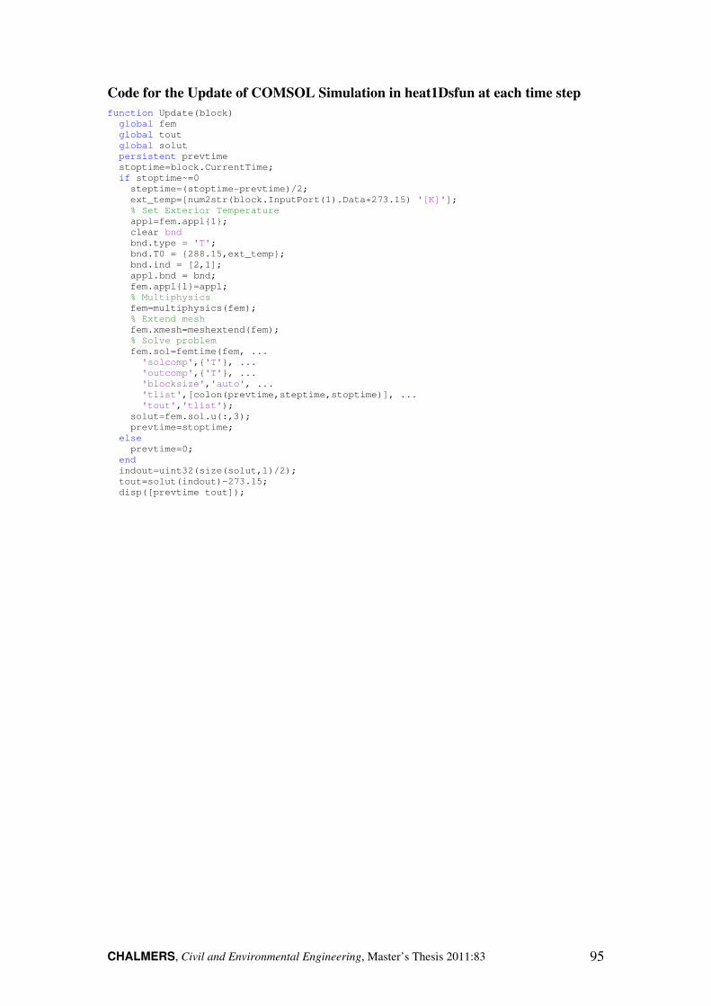
CHALMERS, Civil and Environmental Engineering, Master’s Thesis 2011:83 95
Code for the Update of COMSOL Simulation in heat1Dsfun at each time step function Update(block)
global fem
global tout
global solut
persistent prevtime
stoptime=block.CurrentTime;
if stoptime~=0
steptime=(stoptime-prevtime)/2;
ext_temp=[num2str(block.InputPort(1).Data+273.15) '[K]'];
% Set Exterior Temperature
appl=fem.appl{1};
clear bnd
bnd.type = 'T';
bnd.T0 = {288.15,ext_temp};
bnd.ind = [2,1];
appl.bnd = bnd;
fem.appl{1}=appl;
% Multiphysics
fem=multiphysics(fem);
% Extend mesh
fem.xmesh=meshextend(fem);
% Solve problem
fem.sol=femtime(fem, ...
'solcomp',{'T'}, ...
'outcomp',{'T'}, ...
'blocksize','auto', ...
'tlist',[colon(prevtime,steptime,stoptime)], ...
'tout','tlist');
solut=fem.sol.u(:,3);
prevtime=stoptime;
else
prevtime=0;
end
indout=uint32(size(solut,1)/2);
tout=solut(indout)-273.15;
disp([prevtime tout]);

CHALMERS, Civil and Environmental Engineering, Master’s Thesis 2011:83 96
Appendix C S–function of Underground Heat
Exchangers
Model of Horizontal Pipe in the Ground
Function Name: SinglePipeHoriz_sfun.m
The model developed in Section 4.3.1 was saved as a model m–file and then modified
into an S–function. The function consists of the main model m–file
‘SinglePipeHoriz_sfun.m’ along with a file containing a list of constants and
parameter, ‘SinglePipeHoriz_constants.m’. The constants and parameters file is
shown below.
% SinglePipeHoriz_constants.m %Static Parameters that are parameters of s–function horiz_pipe.pipelength=200; %length of the pipe horiz_pipe.pipedepth=2; % depth of pipe from the ground surface horiz_pipe.soilspace=20; % space of ground around the pipe in all % horizontal directions and in depth
% Variables for Horizontal Pipe Simulation horiz_pipe.L0='0.207'; %circumference of the pipe [m] horiz_pipe.alpha0='140'; %heat transfer coefficient from fluid to soil [W/(m2K)] horiz_pipe.Tgin='9.8[degC]'; %initial ground temperature [°C] horiz_pipe.Ti='9.8[degC]'; %initial inlet temperature of the pipe [°C] horiz_pipe.xarea='0.002827'; %cross sectional area of the pipe [°C] horiz_pipe.flow_velocity='0.2'; %velocity of the fluid in the pipe [m/s] horiz_pipe.Tsoiltop='9.8[degC]'; % initial exterior temperature at soil surface [°C] horiz_pipe.Tsoilbottom='12[degC]'; %initial and long term temperature of ground [°C] horiz_pipe.k_ground='2[W/(m*K)]'; % conductivity of the ground [W/(m*K)] horiz_pipe.rho_ground='1500[kg/m^3]'; % density of the ground [kg/m^3] horiz_pipe.cp_ground='800[J/(kg*K)]'; % heat Capacity of the ground [J/(kg*K)] horiz_pipe.k_fluid='0[W/(m*K)]'; % conductivity of the pipe fluid [W/(m*K)] horiz_pipe.rho_fluid='1000[kg/m^3]'; % density of the pipe fluid [kg/m^3] horiz_pipe.cp_fluid='4200[J/(kg*K)]'; % heat Capacity of the pipe fluid [J/(kg*K)]
% Variables for Mesh horiz_pipe.mesh_geom1_hauto=7; % Auto meshing scale (1= very fine to 8=very coarse) horiz_pipe.mesh_geom2_hmax=5; %maximum size of elements [m]
% Variables for Output horiz_pipe.outputdetails=1; % include output of soil temperatures(1=true)
function SinglePipeHoriz_sfun(block)
% Level-2 M file S-Function for a model of a single horizontal pipe in
% the ground.
setup(block);
%endfunction
function setup(block)
%% Register number of dialog parameters
block.NumDialogPrms = 0;
%% Register number of input and output ports
block.NumInputPorts = 3;
% 3 dynamic inputs - 1. Pipe inlet fluid Temperature [°C]
% 2. Surface temperature of the ground [°C]
% 3. Velocity of the fluid in the pipe [m/s]
block.NumOutputPorts = 1;
%% Setup functional port properties to dynamically inherited.
block.SetPreCompInpPortInfoToDynamic;
block.SetPreCompOutPortInfoToDynamic;
block.InputPort(1).DirectFeedthrough = true;
%% Set block sample time to inherited
block.SampleTimes = [-1 0];
%% Run accelerator on TLC
block.SetAccelRunOnTLC(false);
%% Register methods

CHALMERS, Civil and Environmental Engineering, Master’s Thesis 2011:83 97
block.RegBlockMethod('PostPropagationSetup', @DoPostPropSetup);
block.RegBlockMethod('Outputs', @Output);
block.RegBlockMethod('Update', @Update);
% Global variables
global tout
global solut
global xfem
global flagoutputdetails
% call file with constant parameters of model
SinglePipeHoriz_constants
flagoutputdetails=horiz_pipe.outputdetails;
%% Control Parameters
pipelength= horiz_pipe.pipelength;
pipedepth= horiz_pipe.pipedepth;
soilspace= horiz_pipe.soilspace;
strdomainwidth=num2str(soilspace*2);
strsoildepth=num2str(pipedepth+soilspace);
stryloc=num2str(-soilspace);
strdepthloc=num2str(-pipedepth-soilspace);
strdomainlength=num2str(pipelength+soilspace*2);
%% Beginning of COMSOL generated code
%% COMSOL version
clear vrsn
vrsn.name = 'COMSOL 3.5';
vrsn.ext = 'a';
vrsn.major = 0;
vrsn.build = 608;
vrsn.rcs = '$Name: v35ap $';
vrsn.date = '$Date: 2009/05/11 07:38:49 $';
xfem.version = vrsn;
% turn off COMSOL Simulation progress window
flreport('off')
%% Constants – modified from COMSOL generated code
xfem.const = {'L0',horiz_pipe.L0, ...
'alpha0',horiz_pipe.alpha0, ...
'Tgin',horiz_pipe.Tgin, ...
'Ti',horiz_pipe.Ti, ...
'xarea',horiz_pipe.xarea, ...
'flow_velocity',horiz_pipe.flow_velocity, ...
'Tsoiltop',horiz_pipe.Tsoiltop, ...
'Tsoilbottom',horiz_pipe.Tsoilbottom, ...
'Tsoiltop2',horiz_pipe.Tsoiltop, ...
'k_ground',horiz_pipe.k_ground, ...
'rho_ground',horiz_pipe.rho_ground, ...
'cp_ground',horiz_pipe.cp_ground, ...
'k_fluid',horiz_pipe.k_fluid, ...
'rho_fluid',horiz_pipe.rho_fluid, ...
'cp_fluid',horiz_pipe.cp_fluid};
%% Geometry and Mesh
% Geometry 1
flclear fem
clear draw
g1=block3(strdomainlength,strdomainwidth,strsoildepth,'base','corner','pos',{'0',stryl
oc,strdepthloc},'axis',{'0','0','1'},'rot','0');
g2=curve3([soilspace,pipelength+soilspace],[0,0],[-pipedepth,-pipedepth]);
draw.s.objs = {g1};
draw.s.name = {'BLK1'};
draw.s.tags = {'g1'};
draw.c.objs = {g2};
draw.c.name = {'B1'};
draw.c.tags = {'g2'};
fem.draw = draw;
fem.geom = geomcsg(fem);
fem.mesh=meshinit(fem, ...
'hauto',horiz_pipe.mesh_geom1_hauto);
xfem.fem{1}=fem;
% Geometry 2
flclear fem
clear draw
g3=solid1([0,pipelength]);
draw.s.objs = {g3};
draw.s.name = {'I1'};
draw.s.tags = {'g3'};
fem.draw = draw;
fem.geom = geomcsg(fem);
fem.mesh=meshinit(fem, ...
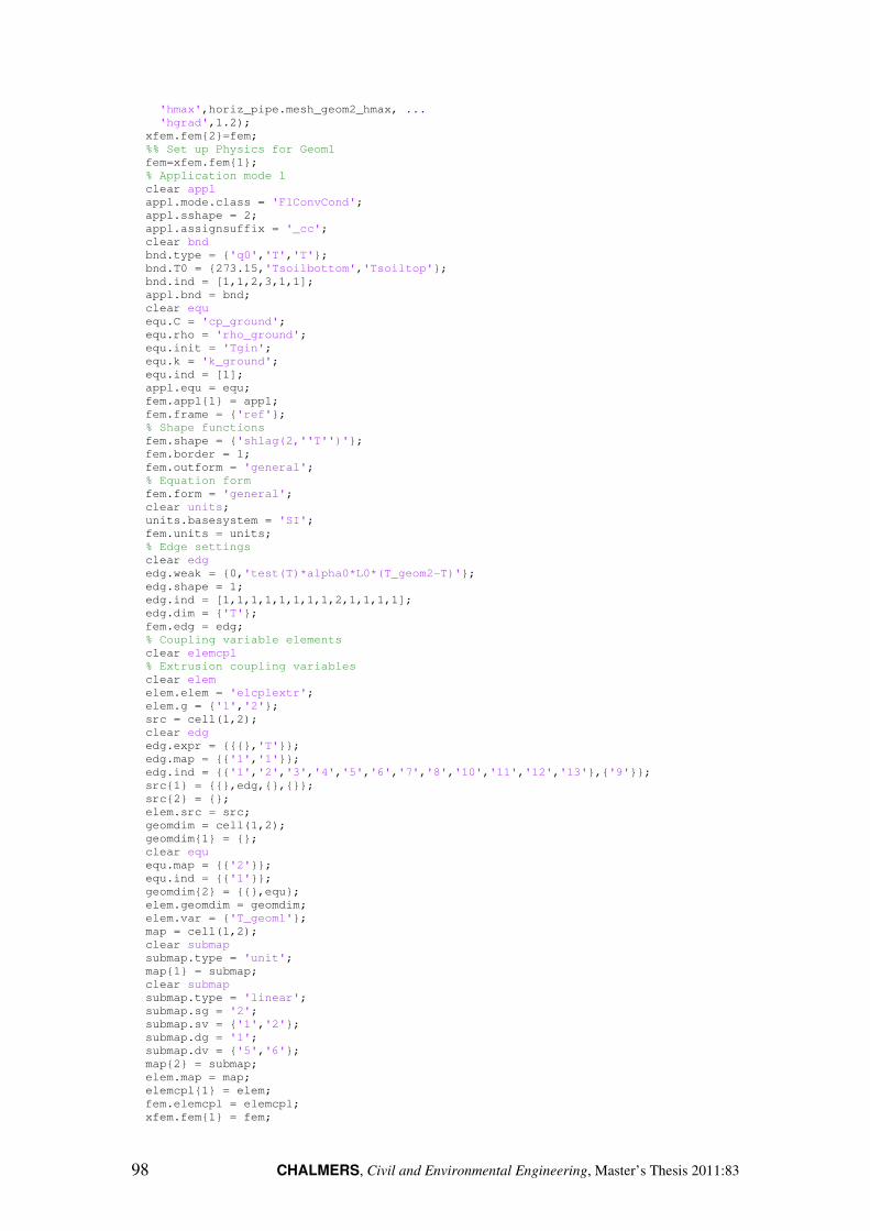
CHALMERS, Civil and Environmental Engineering, Master’s Thesis 2011:83 98
'hmax',horiz_pipe.mesh_geom2_hmax, ...
'hgrad',1.2);
xfem.fem{2}=fem;
%% Set up Physics for Geom1
fem=xfem.fem{1};
% Application mode 1
clear appl
appl.mode.class = 'FlConvCond';
appl.sshape = 2;
appl.assignsuffix = '_cc';
clear bnd
bnd.type = {'q0','T','T'};
bnd.T0 = {273.15,'Tsoilbottom','Tsoiltop'};
bnd.ind = [1,1,2,3,1,1];
appl.bnd = bnd;
clear equ
equ.C = 'cp_ground';
equ.rho = 'rho_ground';
equ.init = 'Tgin';
equ.k = 'k_ground';
equ.ind = [1];
appl.equ = equ;
fem.appl{1} = appl;
fem.frame = {'ref'};
% Shape functions
fem.shape = {'shlag(2,''T'')'};
fem.border = 1;
fem.outform = 'general';
% Equation form
fem.form = 'general';
clear units;
units.basesystem = 'SI';
fem.units = units;
% Edge settings
clear edg
edg.weak = {0,'test(T)*alpha0*L0*(T_geom2-T)'};
edg.shape = 1;
edg.ind = [1,1,1,1,1,1,1,1,2,1,1,1,1];
edg.dim = {'T'};
fem.edg = edg;
% Coupling variable elements
clear elemcpl
% Extrusion coupling variables
clear elem
elem.elem = 'elcplextr';
elem.g = {'1','2'};
src = cell(1,2);
clear edg
edg.expr = {{{},'T'}};
edg.map = {{'1','1'}};
edg.ind = {{'1','2','3','4','5','6','7','8','10','11','12','13'},{'9'}};
src{1} = {{},edg,{},{}};
src{2} = {};
elem.src = src;
geomdim = cell(1,2);
geomdim{1} = {};
clear equ
equ.map = {{'2'}};
equ.ind = {{'1'}};
geomdim{2} = {{},equ};
elem.geomdim = geomdim;
elem.var = {'T_geom1'};
map = cell(1,2);
clear submap
submap.type = 'unit';
map{1} = submap;
clear submap
submap.type = 'linear';
submap.sg = '2';
submap.sv = {'1','2'};
submap.dg = '1';
submap.dv = {'5','6'};
map{2} = submap;
elem.map = map;
elemcpl{1} = elem;
fem.elemcpl = elemcpl;
xfem.fem{1} = fem;
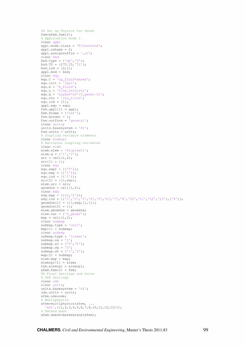
CHALMERS, Civil and Environmental Engineering, Master’s Thesis 2011:83 99
%% Set up Physics for Geom2
fem=xfem.fem{2};
% Application mode 1
clear appl
appl.mode.class = 'FlConvCond';
appl.sshape = 2;
appl.assignsuffix = '_cc';
clear bnd
bnd.type = {'qc','T'};
bnd.T0 = {273.15,'Ti'};
bnd.ind = [2,1];
appl.bnd = bnd;
clear equ
equ.C = 'cp_fluid*xarea';
equ.init = 'Tgin';
equ.k = 'k_fluid';
equ.u = 'flow_velocity';
equ.Q = 'alpha0*L0*(T_geom1-T)';
equ.rho = 'rho_fluid';
equ.ind = [1];
appl.equ = equ;
fem.appl{1} = appl;
fem.frame = {'ref'};
fem.border = 1;
fem.outform = 'general';
clear units;
units.basesystem = 'SI';
fem.units = units;
% Coupling variable elements
clear elemcpl
% Extrusion coupling variables
clear elem
elem.elem = 'elcplextr';
elem.g = {'1','2'};
src = cell(1,2);
src{1} = {};
clear equ
equ.expr = {{'T'}};
equ.map = {{'1'}};
equ.ind = {{'1'}};
src{2} = {{},equ};
elem.src = src;
geomdim = cell(1,2);
clear edg
edg.map = {{{},'2'}};
edg.ind = {{'1','2','3','4','5','6','7','8','10','11','12','13'},{'9'}};
geomdim{1} = {{},edg,{},{}};
geomdim{2} = {};
elem.geomdim = geomdim;
elem.var = {'T_geom2'};
map = cell(1,2);
clear submap
submap.type = 'unit';
map{1} = submap;
clear submap
submap.type = 'linear';
submap.sg = '1';
submap.sv = {'5','6'};
submap.dg = '2';
submap.dv = {'1','2'};
map{2} = submap;
elem.map = map;
elemcpl{1} = elem;
fem.elemcpl = elemcpl;
xfem.fem{2} = fem;
%% Final Settings and Solve
% ODE Settings
clear ode
clear units;
units.basesystem = 'SI';
ode.units = units;
xfem.ode=ode;
% Multiphysics
xfem=multiphysics(xfem, ...
'edl',{[1,2,3,4,5,6,7,8,10,11,12,13]});
% Extend mesh
xfem.xmesh=meshextend(xfem);
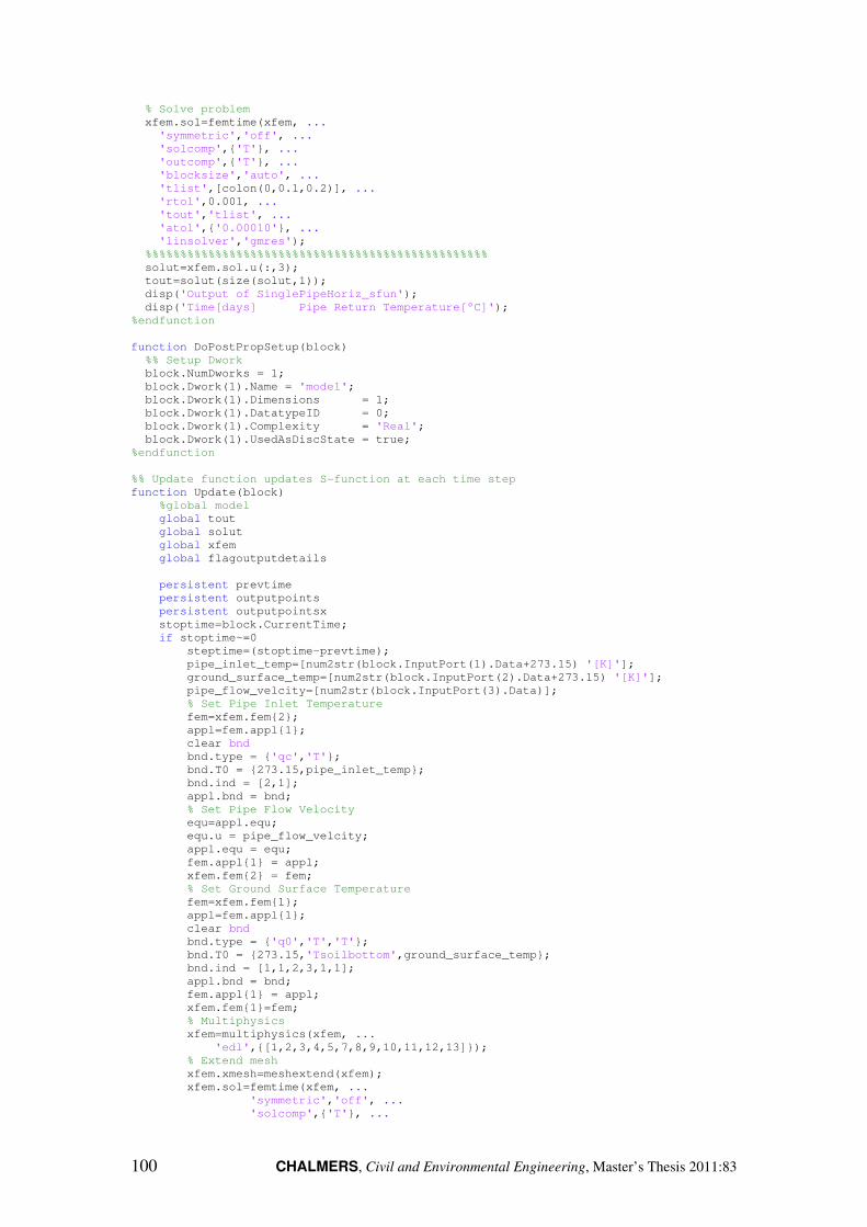
CHALMERS, Civil and Environmental Engineering, Master’s Thesis 2011:83 100
% Solve problem
xfem.sol=femtime(xfem, ...
'symmetric','off', ...
'solcomp',{'T'}, ...
'outcomp',{'T'}, ...
'blocksize','auto', ...
'tlist',[colon(0,0.1,0.2)], ...
'rtol',0.001, ...
'tout','tlist', ...
'atol',{'0.00010'}, ...
'linsolver','gmres');
%%%%%%%%%%%%%%%%%%%%%%%%%%%%%%%%%%%%%%%%%%%%%%%%%
solut=xfem.sol.u(:,3);
tout=solut(size(solut,1));
disp('Output of SinglePipeHoriz_sfun');
disp('Time[days] Pipe Return Temperature[°C]');
%endfunction
function DoPostPropSetup(block)
%% Setup Dwork
block.NumDworks = 1;
block.Dwork(1).Name = 'model';
block.Dwork(1).Dimensions = 1;
block.Dwork(1).DatatypeID = 0;
block.Dwork(1).Complexity = 'Real';
block.Dwork(1).UsedAsDiscState = true;
%endfunction
%% Update function updates S-function at each time step
function Update(block)
%global model
global tout
global solut
global xfem
global flagoutputdetails
persistent prevtime
persistent outputpoints
persistent outputpointsx
stoptime=block.CurrentTime;
if stoptime~=0
steptime=(stoptime-prevtime);
pipe_inlet_temp=[num2str(block.InputPort(1).Data+273.15) '[K]'];
ground_surface_temp=[num2str(block.InputPort(2).Data+273.15) '[K]'];
pipe_flow_velcity=[num2str(block.InputPort(3).Data)];
% Set Pipe Inlet Temperature
fem=xfem.fem{2};
appl=fem.appl{1};
clear bnd
bnd.type = {'qc','T'};
bnd.T0 = {273.15,pipe_inlet_temp};
bnd.ind = [2,1];
appl.bnd = bnd;
% Set Pipe Flow Velocity
equ=appl.equ;
equ.u = pipe_flow_velcity;
appl.equ = equ;
fem.appl{1} = appl;
xfem.fem{2} = fem;
% Set Ground Surface Temperature
fem=xfem.fem{1};
appl=fem.appl{1};
clear bnd
bnd.type = {'q0','T','T'};
bnd.T0 = {273.15,'Tsoilbottom',ground_surface_temp};
bnd.ind = [1,1,2,3,1,1];
appl.bnd = bnd;
fem.appl{1} = appl;
xfem.fem{1}=fem;
% Multiphysics
xfem=multiphysics(xfem, ...
'edl',{[1,2,3,4,5,7,8,9,10,11,12,13]});
% Extend mesh
xfem.xmesh=meshextend(xfem);
xfem.sol=femtime(xfem, ...
'symmetric','off', ...
'solcomp',{'T'}, ...

CHALMERS, Civil and Environmental Engineering, Master’s Thesis 2011:83 101
'outcomp',{'T'}, ...
'blocksize','auto', ...
'tlist',[colon(prevtime,steptime,stoptime)], ...
'init',solut,...
'rtol',0.0001, ...
'tout','tlist', ...
'atol',{'0.000010'}, ...
'linsolver','gmres');
solut=xfem.sol.u(:,2);
prevtime=stoptime;
if flagoutputdetails==1
[outputdata,pe]=postinterp(xfem,'T',outputpoints);
outputdata=outputdata-273.15;
fid =fopen('SingleHorizPipe_ground_output.txt', 'a+');
fprintf(fid,'%e\t',stoptime);
fprintf(fid, '%e\t', outputdata);
fprintf(fid, '\r');
fclose(fid);
[outputdata,pe]=postinterp(xfem,'T',outputpointsx,'Geomnum',2);
outputdata=outputdata-273.15;
fid =fopen('InfSingleUPipe_pipe_output.txt', 'a+');
fprintf(fid,'%e\t',stoptime);
fprintf(fid, '%e\t', outputdata);
fprintf(fid, '\r');
fclose(fid);
end
else
prevtime=0;
if flagoutputdetails==1
SinglePipeHoriz_constants
pipelength= horiz_pipe.pipelength;
pipedepth= horiz_pipe.pipedepth;
soilspace= horiz_pipe.soilspace;
[outputcoord.x,outputcoord.y,outputcoord.z]=meshgrid( ...
soilspace:(pipelength/7):(soilspace+pipelength), ...
0:(soilspace/6):(soilspace/2), ...
((-soilspace/2)-pipedepth):soilspace/6:-pipedepth);
outputpoints=[outputcoord.x(:)';outputcoord.y(:)';outputcoord.z(:)'];
outputpointsx=[soilspace:(pipelength/7):(soilspace+pipelength)];
fid =fopen('SingleHorizPipe_ground_output.txt', 'a+');
fprintf(fid, 'Sfunction Output: Ground Temperature \r')
for iline=1:3
fprintf(fid, '\t')
fprintf(fid, '%e\t', outputpoints(iline,:));
fprintf(fid, '\r');
end
fclose(fid);
fid =fopen('SingleHorizPipe_pipe_output.txt', 'a+');
fprintf(fid, 'Sfunction Output: Pipe Temperature [°C] \r')
fprintf(fid, '\t')
fprintf(fid, '%e\t', outputpointsx(:));
fprintf(fid, '\r');
fclose(fid);
end
end
tout=solut(size(solut,1));
disp([num2str(prevtime/3600/24) ' ' num2str(tout)]);
%endfunction
function Output(block)
global tout
block.OutputPort(1).Data = tout-273.15;
%endfunction

CHALMERS, Civil and Environmental Engineering, Master’s Thesis 2011:83 102
Model of BHEs
The models developed in Section 4.3.2 were saved as a model m–file and then
modified into an S–function. The functions each consists of the main model m–file
along with a file containing a list of constants and parameters as shown in Table 4.6.
An example of the constants and parameters file is shown below. The main model S–
functions are not shown, as they are similar to the model of the horizontal pipe shown
above.
File with Constants: InfSingleUpipe_constants.m
%General Parameters U_pipe.upipelength=200; % length of the bore hole [m] U_pipe.upipecover=2; % depth of pipe from the ground surface [m] U_pipe.soilspace=20; % space of ground around the pipe in all % horizontal directions and in depth [m] U_pipe.boreholediameter=0.13; %diameter of the borehole [m] U_pipe.relativepipelocation=0.8; % relative location of % pipes in borehole [-] ((relativepipelocation=distance of pipe from % centre of bore hole)/(radius of borehole)) U_pipe.TsoilinitialdegC=9.8; % initial ground temperature [°C] U_pipe.pipesspace=6; % space between pipes [m]
% Variables for Simulation U_pipe.L0='0.1257'; %circumference of the pipe [m] U_pipe.alpha0='164'; %heat transfer coefficient from fluid to soil [W/(m2K)] U_pipe.Tgin='10[degC]'; %initial ground temperature [°C] U_pipe.Ti='10[degC]'; %initial inlet temperature of the pipe [°C] U_pipe.xarea='0.0012566'; %cross sectional area of the pipe [°C] U_pipe.flow_velocity='0.6'; %velocity of the fluid in the pipe [m/s] U_pipe.Tsoiltop='9.8[degC]'; % initial exterior temperature at soil surface [°C] U_pipe.Tsoilbottom='9.8[degC]'; %initial and long term temperature of ground [°C] U_pipe.k_ground='3.5[W/(m*K)]'; % conductivity of the ground [W/(m*K)] U_pipe.rho_ground='2000[kg/m^3]'; % density of the ground [kg/m^3] U_pipe.cp_ground='1000[J/(kg*K)]'; % heat Capacity of the ground [J/(kg*K)] U_pipe.k_grout='2.0[W/(m*K)]'; % conductivity of the grout [W/(m*K)] U_pipe.rho_grout='2000[kg/m^3]'; % density of the grout [kg/m^3] U_pipe.cp_grout='1000[J/(kg*K)]'; % heat Capacity of the grout [J/(kg*K)] U_pipe.k_fluid='0[W/(m*K)]'; % conductivity of the pipe fluid [W/(m*K)] U_pipe.rho_fluid='1000[kg/m^3]'; % density of the pipe fluid [kg/m^3] U_pipe.cp_fluid='4200[J/(kg*K)]'; % heat Capacity of the pipe fluid [J/(kg*K)]
% Variables for Mesh % Variables for 3D ground mesh U_pipe.mesh_geom1_hauto=8; % Auto meshing scale (1= very fine to 8=very coarse) U_pipe.mesh_geom1_xscale=20; % relative scaling in x direction U_pipe.mesh_geom1_yscale=20; % relative scaling in y direction % Variables for 1D pipe elements U_pipe.mesh_geom2_hmax=4; %maximum size of elements [m]
% Variables for Ground Temperature Output U_pipe.outputdetails=1; % include output of soil temperatures(1=true)
Related Documents