Modelling the Internet Delay Space Based on Geographical Locations

Modelling the Internet Delay Space Based on Geographical Locations

Sebastian Kaune∗, Konstantin Pussep∗, Christof Leng∗, Aleksandra Kovacevic∗,Gareth Tyson†, and Ralf Steinmetz∗

∗ Technische Universitat Darmstadt, Germany† Lancaster University, United Kingdom

Abstract

Existing approaches for modelling the Internet delayspace predict end-to-end delays between two arbitraryhosts as static values. Further, they do not capturethe characteristics caused by geographical constraints.Peer-to-peer (P2P) systems are, however, often verysensitive to the underlying delay characteristics of theInternet, since these characteristics directly influencesystem performance.

This work proposes a model to predict lifelike delaysbetween a given pair of end hosts. In addition to itslow delay computation time, it has only linear memorycosts which allows large scale P2P simulations to beperformed. The model includes realistic delay jitter,subject to the geographical position of the sender andthe receiver. Our analysis, using existing Internet mea-surement studies reveals that our approach seems to bean optimal tradeoff between a number of conflictingproperties of existing approaches.

1. Introduction

Peer-to-peer (P2P) systems have gained significantresearch attention in recent years. Due to their large-scale, simulation is often the most appropriate evalu-ative method. Internet properties, and especially theirdelay characteristics, often directly influence P2P sys-tem performance. In delay-optimized overlays, for in-stance, proximity neighbor selection (PNS) algorithmsselect the closest node in the underlying network fromamong those that are considered equivalent by therouting table. The definition of closeness is typicallyround-trip time (RTT). In addition, having realisticdelay cluster properties is equally important whenanalyzing caching strategies and server placement po-lices. Therefore, in order to obtain accurate results,simulations must include an adequate model of theInternet delay space.

The main challenges in creating such a model canbe summarized as follows: (i) The model must be ableto predict lifelike delays between a given pair of end-hosts. (ii) The model must include realistic delay jitter.Normally, the propagation of messages is affected bythe processing and queuing delays of intermediaterouters, something which varies over time. Therefore,end-to-end delays vary between two arbitrary nodesand are therefore non-static.

We argue that both requirements are subject to thegeographical position of the sender and the receiver.First, the minimal delay is limited by the propaga-tion speed of signals in the involved links whichincreases proportionally with the link length. Second,the Internet infrastructure is very different in differentcountries. As long-term measurement studies (cf. Sec.3.1) reveal, jitter and packet loss rates are heavilyinfluenced by the location of participating nodes. Forexample, the routers in a developing country are morelikely to suffer from overload than those in a moreeconomically advanced country. Such observations aretypical for real-world measurement data but are absentin artificial delay models that ignore geographicallocations.

The main contribution of this paper is the provisionof a predictive model of the Internet delay space thatfulfils the above stated requirements. To do so, weuse rich data from two measurement projects as input.The resulting delays are non-static, and realisticallyreflect the delay characteristics caused by the geo-graphical constraints. Additionally, we compare ourmodel against the existing approaches of obtainingend-to-end delays. To this end, we show that our calcu-lated distance of non-measured links is also a suitablerepresentation of delays occurring in the Internet. Thecomplexity of our model is O(n) which is acceptablefor the inherent memory constraints of large scalesimulations.

In Section 2 we give an overview of the state-of-the art Internet delay models. Section 3 describes the

data sets we use and the assumptions we make. Finally,our model is presented in Section 4 and evaluated inSection 5. Concluding remarks are given in Section 6.

2. Related WorkCurrently, there are three different approaches to

obtaining a delay model for P2P-related simulations.The first approach uses the King tool [1] to computethe all-pair end-to-end delays among a large numberof globally distributed DNS servers. In more detail,each server is typically located in a distinct domain,and the measured delays therefore represent the staticInternet delay space among the edge networks. Dueto the quadratic time requirement for collecting thisdata, the size of the resulting delay matrix is oftenlimited. For example, [1] provides a delay matrix with1740 rows/columns. This is a non-trivial amount ofmeasurement data to obtain. Delay synthesizers usethis statistical data as an input to produce Internet delayspaces at a large scale [2].

The second approach is based on using artificial linkdelays assigned by topology generators such as Inet[3] or GT-ITM [4]. Within this approach, a topologyfile is initially generated for a pre-defined numberof nodes. The end-to-end delay is then computed onthe fly by determining the topology’s all-pair shortest-path; a process which requires high computationalpower. Alternatively, pre-computation of an all-pairdelay matrix squares the memory overhead to O(n2).

The third approach is to start with the data of Inter-net measurement projects, e.g. Surveyor [5], CAIDA[6], and AMP [7]. These projects typically performactive probing to up to a million destination hosts,derived from a small number of globally distributedmonitor hosts. Prior work uses this data as an input togenerate realistic delay by embedding hosts into a lowdimensional Euclidean space [8].

This work follows the third approach of obtainingend-to-end delays. However, our approach differs torecent work in the following two major points. First,none of the aforementioned approaches considers re-alistic delay jitter. That is, recent approaches aim topredict static delays, either the average or minimumdelay between two hosts. Second, most of prior workdoes not accurately reflect delay characteristics causedby the different geographical regions of the world. Thisissue can, however, highly influence the performanceof P2P systems, as we will see later on.

3. Data Collection and Assumptions

This section provides background information onthe measured Internet delay data we use in this work.

Finally, the assumptions on which our delay model isbased on are given.

3.1. Data from two Internet measurementprojects

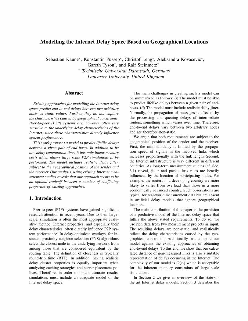
We use two kinds of data for this work. Firstly,we utilise the measurement data of the CAIDA’smacroscopic topology probing project from August2007 [6]. This data contains a large volume of RTTmeasurements taken between 20 globally distributedmonitor hosts and nearly 400,000 destination hosts.Within this project, each monitor actively probes everyhost stored in the so-called destination list by sendingICMP [9] echo-requests. This lists account for 313,471hosts covering the routable IPv4 space, alongside58,312 DNS clients. Each monitor-to-destination linkis measured 5-10 times a month, resulting in an overallamount of 40 GB of measurement data. Fig. 1(a)plots this data in relation to the geographical distancebetween each monitor host and its destinations. Both,the geographical locations of the monitors and thedestination hosts are determined by MaxMind GeoIPservice1 [10]. It can be observed that there is a propor-tionality of the RTT to the length of the transmissionmedium. Also, the figure clearly shows the impact ofthe queuing/processing delays caused by intermediaterouters. The ’islands’ at 8000 - 12000 km and 300 -400 ms RTT arises from countries in Africa and SouthAsia.

To study the changes of delay over time, we ad-ditionally incorporate the data of the PingER project[11]. This project currently has more than 40 mon-itoring sites in 20 countries and about 670 destina-tion sites in 150 countries in most regions of theworld. Compared to the CAIDA project, the numberof monitor sites is significantly higher and globallymore distributed whereas the amount of remote sitesis by order of magnitudes smaller. Nevertheless, theRTT for one monitor-to-destination link is measuredup to 960 times a day, in contrast to 5-10 times permonth by the CAIDA project. As seen later on, thisallows us to accurately predict the inter-packet delayvariation between any two hosts located in differentregions, countries or continents.

3.2. Assumptions

As already stated before, the CAIDA projectmeasures RTTs containing the end-to-end delay of

1. The obviously impossible RTT values below the propagationtime of the speed of light in fiber can be explained by a falsepositioning through MaxMind.

0

100

200

300

400

500

600

700

800

0 5000 10000 15000 20000

Me

asu

red

ro

un

d-t

rip

tim

e (

in m

sec)

Distance (in kilometres)

Speed of light in fiberLinear regression (world)

(a)

MaxMind

H1 = <(x1, … xn), GeoData>

HN = <(x1, … xn), GeoData>

Host set with GeoData

Embedding into Euclidean space

…

End-to-end-link jiiter distribution

H1

H2

60 ms PingER

60 ms

CAIDA

Simulation Framework

MinimumRTT2

Delay(H1, H2) = + Jitter

Static part Random part

(b)

Figure 1. The measured round-trip times in relation to the geographical distance in August 2007 (left).Overview about our delay space modeling techniques (right).

monitor-to-destination links, but also the transmissionand processing delay of the destination host whenreceiving the echo-request and sending the echo-reply.We assume for the remainder of this paper, that theend-to-end delay can be calculated by dividing themeasured RTT by two whilst neglecting the lattertwo delays. This is a reasonable assumption since thesize of the echo packet is only 52 bytes. Also, theprocessing delay on the destination host is usually inthe range of nanoseconds, and is therefore negligible.

4. ModelThis section details our model that aims to realisti-

cally predict end-to-end delays between two arbitraryhosts chosen from a predefined host set. These delaysare non-static, and consider the geographical locationof both the source and destination host. Further, themodel properties in terms of computation and memoryoverhead are given.

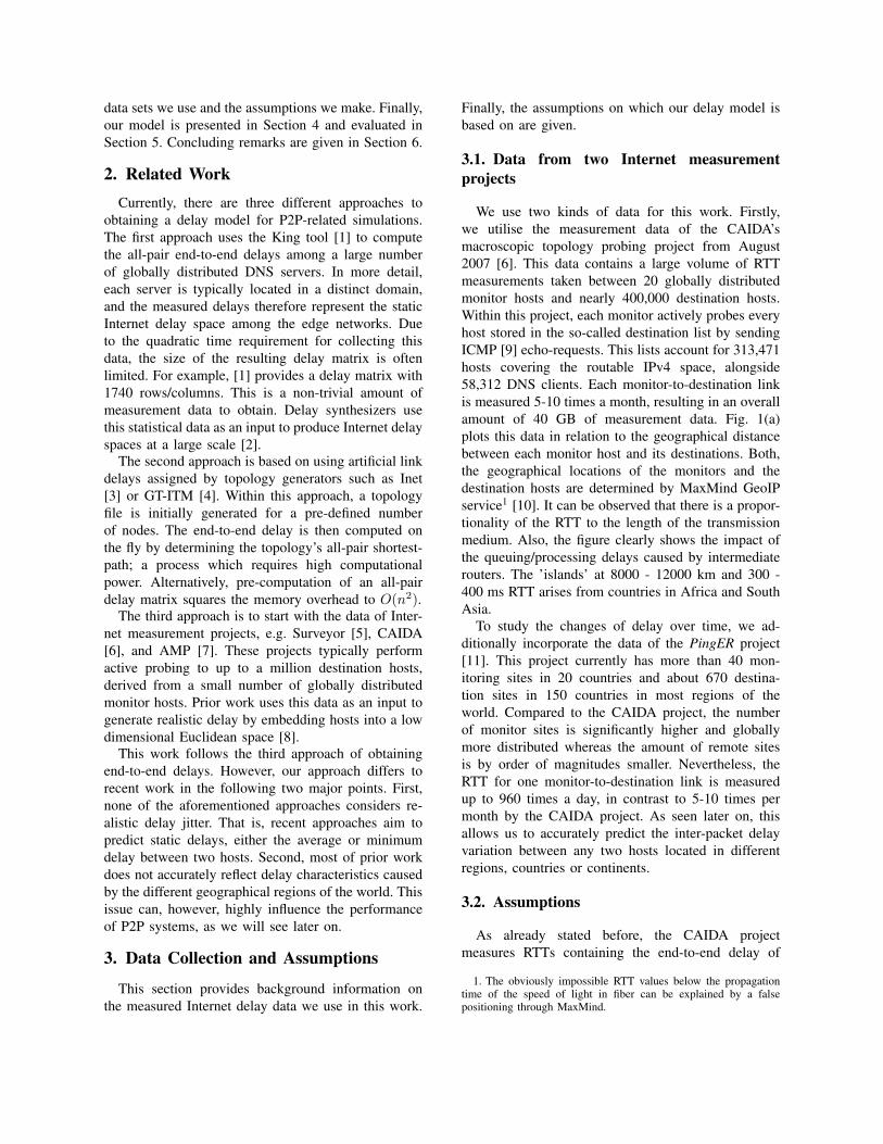
4.1. OverviewWe split up the modelling of delay into a two-

part architecture. The first part computes the minimumdelay between any two hosts based on the measuredround-trip time samples of CAIDA, and is thereforestatic. The second part, on the other hand, is variableand determines the inter-packet delay variation of thisminimum delay, also known as jitter.

Thus, the end-to-end delay between two hosts H1

and H2 is then given by

delay(H1,H2) =minimumRTT

2+ jitter (1)

Fig. 1(b) gives an overview of our two part delayspace modelling techniques. The first part (top left)generates a set of hosts from which the simulation

framework can choose a subset from. More precisely,this set is composed of the destination list of theCAIDA measurement project. Using the MaxMindGeoIP database, we are able to look up the IP ad-dresses of these hosts and find out their geographicposition, i.e., continent, country, region, and ISP. Inorder to calculate the minimum delay between any twohosts, the Internet is modelled as a multidimensionalEuclidean spaceS. Each host is then characterized bya point in this space so that the minimum round-triptime between any two nodes can be predicted by awell-defined distance function.

The second part (top right), on the other hand, deter-mines the inter-packet delay variation of this minimumdelay; it uses the rich data of the PingER project toreproduce end-to-end link jitter distributions. Thesedistributions can then be used to calculate random jittervalues at simulation runtime.

Basically, both parts of our architecture require anoffline computation phase to prepare the data neededfor the simulation framework. Our overall goal is thento have a very compact and scalable presentation of theunderlay at simulation runtime without introducing asignificant computational overhead. In the following,we describe each part of the architecture in detail.

4.2. Part I: Embedding CAIDA hosts into theEuclidean Space

The main challenge of the first part is to place the setof destination hosts into a multidimensional Euclideanspace, so that the computed minimum round-trip timesapproximate the measured distance as accurately aspossible. To do so, we follow the approach of [12]and apply the technique of global network positioningin a slightly different way. However, this results inan optimization problem of minimizing the sum of

the error between the measured and the calculateddistances.

In the following, we denote the coordinate of ahost H in a D-dimensional coordinate space as cSH =(cSH,1, ..., c

SH,D). The measured round-trip time be-

tween the hosts H1 and H2 is given by dH1H2 whilstthe computed distance dSH1H2

is defined by a distancefunction that operates on those coordinates:

dSH1H2 =√

(cSH1,1− cSH2,1

)2 + ...+ (cSH1,D− cSH2,D

)2

(2)As needed for the minimization problems described

below, we introduce a weighted error function ε(·) tomeasure the quality of each performed embedding:

ε(dH1H2 , dSH1H2) =

(dH1H2 − dSH1H2

dH1H2

)2

(3)

At first, we calculate the coordinates cSL1, ..., cSLN

ofa small sample of N hosts, also known as landmarksL1 to LN . These coordinates then serve as referencepoints with which the position of any destination hostcan be oriented in S. A precondition for the selectedlandmarks is the existence of measured round-triptimes to each other. In our approach, these landmarksare chosen from the set of measurement monitors fromthe CAIDA project, since these monitors fulfil thisprecondition. To this end, we seek to minimize thefollowing objective function fobj1:

fobj1(cSL1 , ..., c

SLN

) =∑

Li,Lj∈{L1,...,LN}|i>j

ε(dLiLj , dSLiLj

)

(4)There are many approaches with different compu-

tational costs that can be applied [12][13]. Previouswork has shown that a five dimensional Euclideanembedding approximates the Internet delay space verywell [14]. Therefore, we select N (=6) monitors out ofall available monitors using the maximum separationmethod [8]. This method determines the subset of Nmonitors out of all available monitors which producesthe maximum sum for all inter-monitor round-triptimes2. Due to the fact that the overall number ofmonitors within the CAIDA project is 20, these moni-tors can easily be obtained through iteration across allcombinations.

In the second step, each destination host is individu-ally (one after the other) embedded into the Euclideanspace. To do this, round-trip time measurements toall N monitor hosts must be available. Similarly tothe previous step, we take the minimum value across

2. Note that we consider only the minimum value across thesamples of inter-monitor RTT measurements

the monitor-to-host RTT samples. While positioningthe destination hosts coordinate into S, we aim tominimize the overall error between the predicted andmeasured monitor-to-host RTT by solving the follow-ing minimization problem fobj2:

fobj2(cSH) =

∑Li∈{L1,...,LN}

ε(dHLi , dSHLi

) (5)

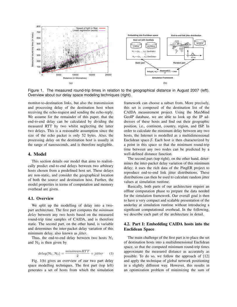
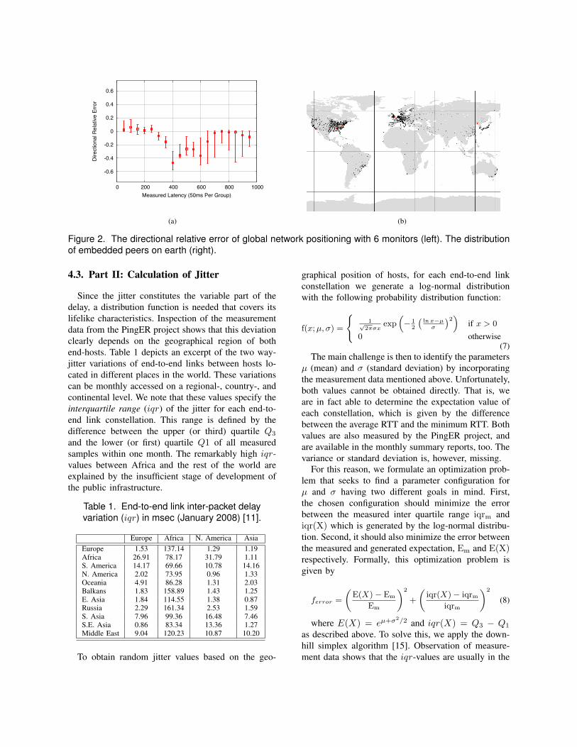
An exact solution of this non-linear optimizationproblem is very complex and computationally inten-sive; we therefore apply an approximate solution thatcan be found by applying the generic downhill simplexalgorithm of Nelder and Mead [15]. Finally, Fig. 2(b)depicts all embedded monitor hosts (red points) anddestination hosts, and their determined geographicallocation on earth.

Once all host coordinates are computed, we use thedirectional relative error r to quantify the quality of theoverall embedding. This metric describes the relativedeviation of the calculated value to the measureddistance, and is defined as

r(dH1H2 , dSH1H2) =

dH1H2 − dSH1H2

min(dH1H2 , dSH1H2

)(6)

A directional relative error of 0 means that themeasured and calculated distances are equal; a valueof 1 indicates that the calculated distance is the halfof the measured one whilst an error of -1 means thatthe calculated distance is double of the measured one.

Fig. 2(a) depicts this error after the positioning ofall the hosts. For this illustration, we consider onlythe measured minimum round-trip times used for ourembedding as stated above. We then classify theminto distinct intervals, each of 50 ms. Afterwards, wecalculate the directional relative error for each interval.The squares depict the interval’s median error, whereasthe vertical lines indicate the 25th percentile and the75th percentile. It can be observed that the embed-ding effectively predicts round-trip times in intervalsbetween (0ms, 300ms]. The quality of the embeddingdecreases, however, for round-trip times in ranges of300ms, 600ms. That is, our embedding tends to overpredict the measured data in these intervals. Neverthe-less, we note that the round-trip times in these intervalsonly account for 5.8% of the measured data.

In this regard, we have also experimented withembeddings in higher dimensional Euclidean spacesreaching up to 11 dimensions. However, we observeonly a very negligible improvement of the qualityof the modelled delay space; the results for 6, 9and 12 selected monitor hosts, creating a 5, 8, and11 dimensional embedding respectively, were nearlyidentical.

-0.6

-0.4

-0.2

0

0.2

0.4

0.6

0 200 400 600 800 1000

Dire

ctio

nal R

elat

ive E

rror

Measured Latency (50ms Per Group)

(a) (b)

Figure 2. The directional relative error of global network positioning with 6 monitors (left). The distributionof embedded peers on earth (right).

4.3. Part II: Calculation of Jitter

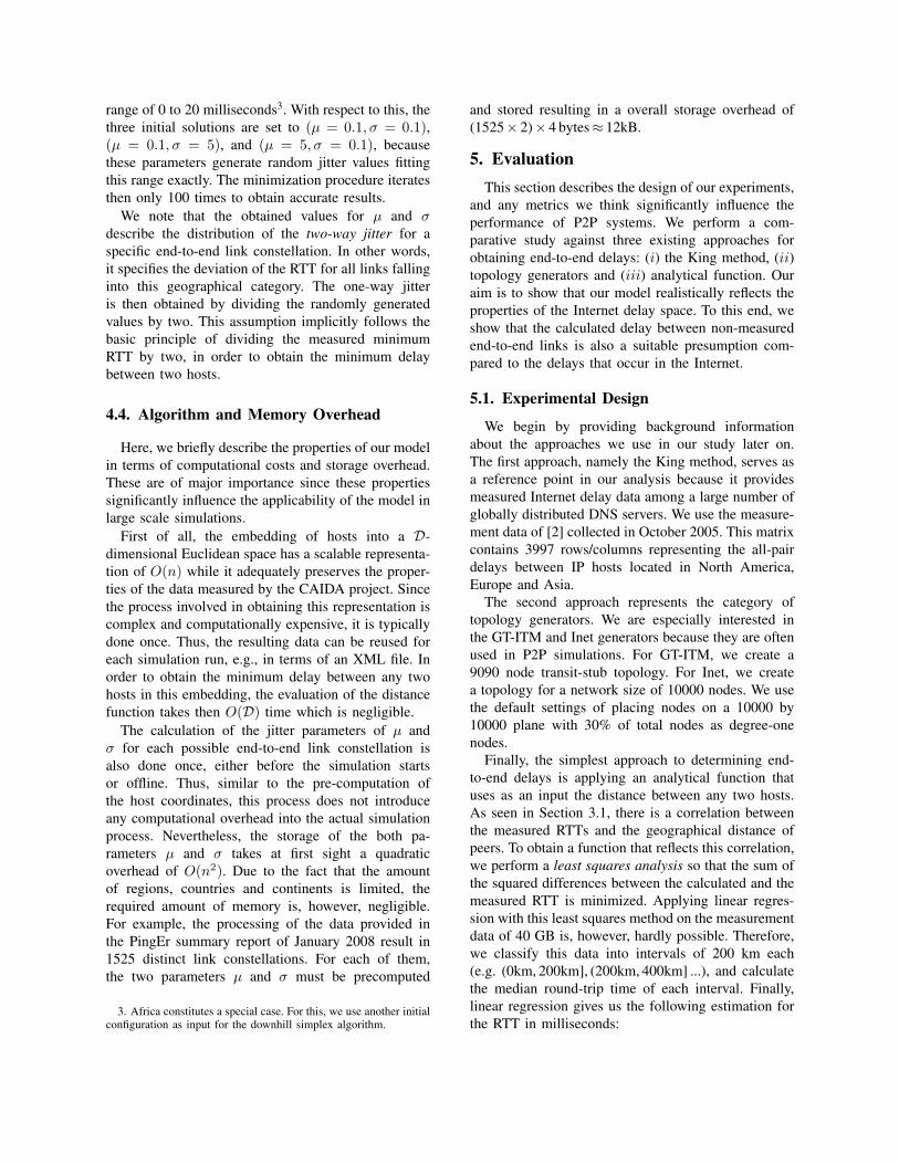
Since the jitter constitutes the variable part of thedelay, a distribution function is needed that covers itslifelike characteristics. Inspection of the measurementdata from the PingER project shows that this deviationclearly depends on the geographical region of bothend-hosts. Table 1 depicts an excerpt of the two way-jitter variations of end-to-end links between hosts lo-cated in different places in the world. These variationscan be monthly accessed on a regional-, country-, andcontinental level. We note that these values specify theinterquartile range (iqr) of the jitter for each end-to-end link constellation. This range is defined by thedifference between the upper (or third) quartile Q3

and the lower (or first) quartile Q1 of all measuredsamples within one month. The remarkably high iqr-values between Africa and the rest of the world areexplained by the insufficient stage of development ofthe public infrastructure.

Table 1. End-to-end link inter-packet delayvariation (iqr) in msec (January 2008) [11].

Europe Africa N. America AsiaEurope 1.53 137.14 1.29 1.19Africa 26.91 78.17 31.79 1.11S. America 14.17 69.66 10.78 14.16N. America 2.02 73.95 0.96 1.33Oceania 4.91 86.28 1.31 2.03Balkans 1.83 158.89 1.43 1.25E. Asia 1.84 114.55 1.38 0.87Russia 2.29 161.34 2.53 1.59S. Asia 7.96 99.36 16.48 7.46S.E. Asia 0.86 83.34 13.36 1.27Middle East 9.04 120.23 10.87 10.20

To obtain random jitter values based on the geo-

graphical position of hosts, for each end-to-end linkconstellation we generate a log-normal distributionwith the following probability distribution function:

f(x;µ, σ) =

{1√

2πσxexp(− 1

2

(ln x−µσ

)2)if x > 0

0 otherwise(7)

The main challenge is then to identify the parametersµ (mean) and σ (standard deviation) by incorporatingthe measurement data mentioned above. Unfortunately,both values cannot be obtained directly. That is, weare in fact able to determine the expectation value ofeach constellation, which is given by the differencebetween the average RTT and the minimum RTT. Bothvalues are also measured by the PingER project, andare available in the monthly summary reports, too. Thevariance or standard deviation is, however, missing.

For this reason, we formulate an optimization prob-lem that seeks to find a parameter configuration forµ and σ having two different goals in mind. First,the chosen configuration should minimize the errorbetween the measured inter quartile range iqrm andiqr(X) which is generated by the log-normal distribu-tion. Second, it should also minimize the error betweenthe measured and generated expectation, Em and E(X)respectively. Formally, this optimization problem isgiven by

ferror =

(E(X)− Em

Em

)2

+

(iqr(X)− iqrm

iqrm

)2

(8)

where E(X) = eµ+σ2/2 and iqr(X) = Q3 − Q1

as described above. To solve this, we apply the down-hill simplex algorithm [15]. Observation of measure-ment data shows that the iqr-values are usually in the

range of 0 to 20 milliseconds3. With respect to this, thethree initial solutions are set to (µ = 0.1, σ = 0.1),(µ = 0.1, σ = 5), and (µ = 5, σ = 0.1), becausethese parameters generate random jitter values fittingthis range exactly. The minimization procedure iteratesthen only 100 times to obtain accurate results.

We note that the obtained values for µ and σdescribe the distribution of the two-way jitter for aspecific end-to-end link constellation. In other words,it specifies the deviation of the RTT for all links fallinginto this geographical category. The one-way jitteris then obtained by dividing the randomly generatedvalues by two. This assumption implicitly follows thebasic principle of dividing the measured minimumRTT by two, in order to obtain the minimum delaybetween two hosts.

4.4. Algorithm and Memory Overhead

Here, we briefly describe the properties of our modelin terms of computational costs and storage overhead.These are of major importance since these propertiessignificantly influence the applicability of the model inlarge scale simulations.

First of all, the embedding of hosts into a D-dimensional Euclidean space has a scalable representa-tion of O(n) while it adequately preserves the proper-ties of the data measured by the CAIDA project. Sincethe process involved in obtaining this representation iscomplex and computationally expensive, it is typicallydone once. Thus, the resulting data can be reused foreach simulation run, e.g., in terms of an XML file. Inorder to obtain the minimum delay between any twohosts in this embedding, the evaluation of the distancefunction takes then O(D) time which is negligible.

The calculation of the jitter parameters of µ andσ for each possible end-to-end link constellation isalso done once, either before the simulation startsor offline. Thus, similar to the pre-computation ofthe host coordinates, this process does not introduceany computational overhead into the actual simulationprocess. Nevertheless, the storage of the both pa-rameters µ and σ takes at first sight a quadraticoverhead of O(n2). Due to the fact that the amountof regions, countries and continents is limited, therequired amount of memory is, however, negligible.For example, the processing of the data provided inthe PingEr summary report of January 2008 result in1525 distinct link constellations. For each of them,the two parameters µ and σ must be precomputed

3. Africa constitutes a special case. For this, we use another initialconfiguration as input for the downhill simplex algorithm.

and stored resulting in a overall storage overhead of(1525× 2)× 4 bytes≈ 12kB.

5. EvaluationThis section describes the design of our experiments,

and any metrics we think significantly influence theperformance of P2P systems. We perform a com-parative study against three existing approaches forobtaining end-to-end delays: (i) the King method, (ii)topology generators and (iii) analytical function. Ouraim is to show that our model realistically reflects theproperties of the Internet delay space. To this end, weshow that the calculated delay between non-measuredend-to-end links is also a suitable presumption com-pared to the delays that occur in the Internet.

5.1. Experimental Design

We begin by providing background informationabout the approaches we use in our study later on.The first approach, namely the King method, serves asa reference point in our analysis because it providesmeasured Internet delay data among a large number ofglobally distributed DNS servers. We use the measure-ment data of [2] collected in October 2005. This matrixcontains 3997 rows/columns representing the all-pairdelays between IP hosts located in North America,Europe and Asia.

The second approach represents the category oftopology generators. We are especially interested inthe GT-ITM and Inet generators because they are oftenused in P2P simulations. For GT-ITM, we create a9090 node transit-stub topology. For Inet, we createa topology for a network size of 10000 nodes. We usethe default settings of placing nodes on a 10000 by10000 plane with 30% of total nodes as degree-onenodes.

Finally, the simplest approach to determining end-to-end delays is applying an analytical function thatuses as an input the distance between any two hosts.As seen in Section 3.1, there is a correlation betweenthe measured RTTs and the geographical distance ofpeers. To obtain a function that reflects this correlation,we perform a least squares analysis so that the sum ofthe squared differences between the calculated and themeasured RTT is minimized. Applying linear regres-sion with this least squares method on the measurementdata of 40 GB is, however, hardly possible. Therefore,we classify this data into intervals of 200 km each(e.g. (0km, 200km], (200km, 400km] ...), and calculatethe median round-trip time of each interval. Finally,linear regression gives us the following estimation forthe RTT in milliseconds:

0

0.2

0.4

0.6

0.8

1

0 200 400 600 800 1000 1200 1400

CD

F

Round-trip time (in msec)

Cambridge, UK (measured)Cambridge, UK (predicted)

Eugene, OR, US (measured)Eugene, OR, US (predicted)

Shenyang, CN (measured)Shenyang, CN (predicted)

(a)

0

0.2

0.4

0.6

0.8

1

0 200 400 600 800 1000 1200 1400

CD

F

Round-trip time (in msec)

GT-ITMInet

(b)

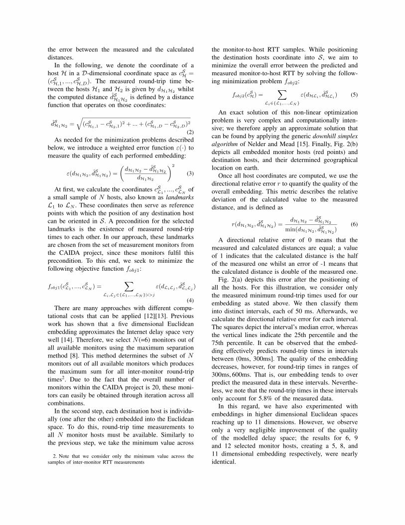
Figure 3. The measured and predicted round-trip time (RTT) distribution as seen from different locations inthe world (left). The RTT distribution as seen from a typical node generated by topology generators (right).

fworld(da,b) = 62 + 0.02 ∗ da,b (9)

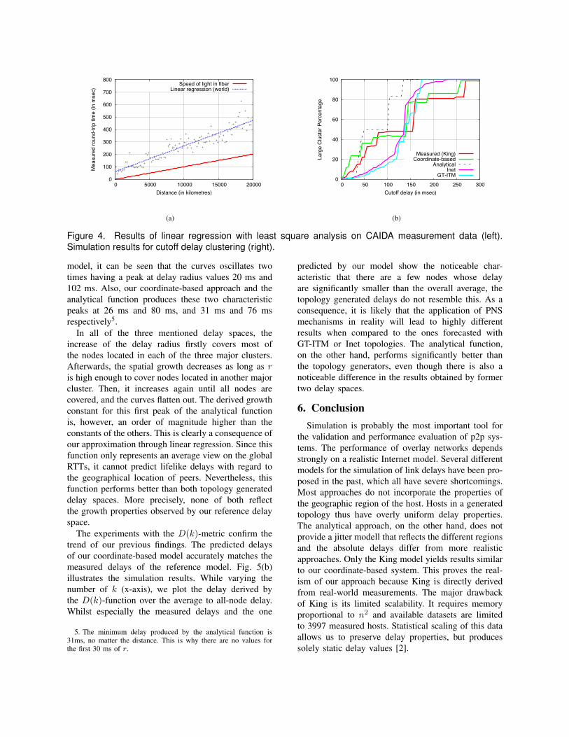
whereas da,b is the distance between two hosts inkilometres. The delay is then given by f(da,b) dividedby two. Fig. 4(a) illustrates this function and thecalculated median RTT times of each interval.

5.2. Metrics

To benchmark the different approaches on theirability to realistically reflect Internet delay character-istics, we apply a set of metrics that are known tosignificantly influence the performance of P2P systems[2]:• Cutoff delay clustering – In the area of P2P content

distribution networks, topologically aware clustering isa very important issue. Nodes are often grouped intoclusters based on their delay characteristics, in order toprovide higher bandwidth and to speed up access [16].The underlying delay model must therefore accuratelyreflect the Internet’s clustering properties. Otherwise,analysis of system performance might lead to wrongconclusions.

To quantify this, we use a clustering algorithmwhich iteratively merges two distinct clusters into alarger one until a cutoff delay value is reached. Inmore detail, at first each host is treated as a singletoncluster. The algorithm then determines the two closestclusters to merge. The notion of closeness between twoclusters is defined as the average delay between allnodes contained in both cluster. The merging processstops if the delay of the two closest clusters exceedsthe predefined cutoff value. Afterwards, we calculatethe fraction of hosts contained in the largest clustercompared to the entire host set under study.

• Spatial growth metric – In many application areasof P2P systems, such as in mobile P2P overlays, thecost of accessing a data object grows as the numberof hops to the object increases. Therefore, it is oftenadvantageous to locate the ’closest’ copy of a dataobject to lower operating costs and reduce responsetimes. Efficient distributed nearest neighbor selectionalgorithms have been proposed to tackle this issuefor growth-restricted metric spaces [17]. In this metricspace, the number of nodes contained in the radius ofdelay r around node p, increases at most by a constantfactor c when doubling this delay radius. Formally,let Bp(r) denote the number of nodes contained in adelay radius r, then Bp(r) ≤ c ·Bp(2r). The functionBp(r)/Bp(2r) can therefore be used to determine thespatial growth c of a delay space.• Proximity metric – In structured P2P overlays

which apply proximity neighbor selection (PNS), over-lay neighbors are selected by locating nearby underlaynodes [18]. Thus, these systems are very sensitiveto the underlying network topology, and especiallyto its delay characteristics. An insufficient model ofthe Internet delay space would result in routing tableentries that do not occur in reality. This would inturn directly influence the routing performance andconclusions might then be misleading. To reflect theneighborhood from the point of view of each host,we use the D(k)-metric. This metric is defined byD(k) = 1

|N |∑p∈N d(p, k), whereas d(p, k) is the

average delay from node p to its k-closest neighborsin the underlying network [19].

5.3. Analysis with measured CAIDA data

Before we compare our system against existingapproaches, we briefly show that our delay model

produces lifelike delays even though their calculationis divided into two distinct parts.

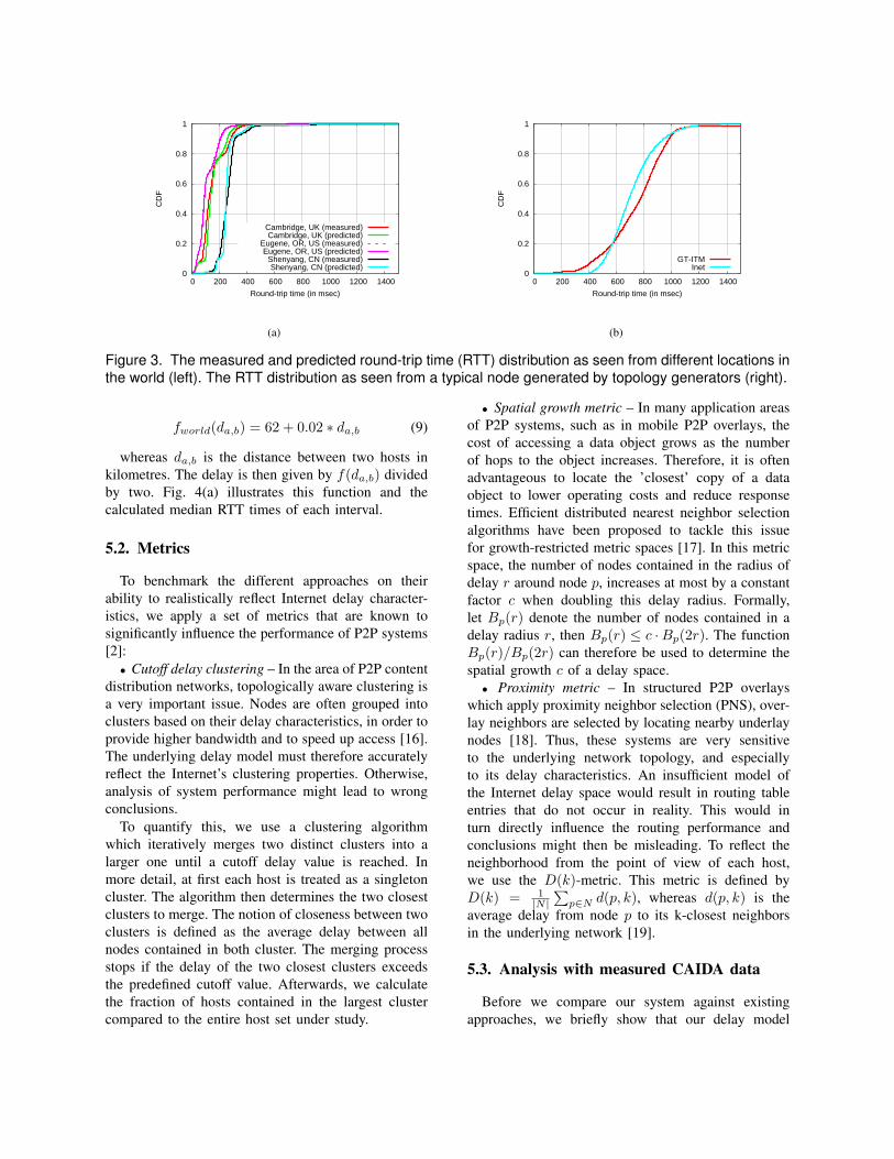
As an illustration of our results, Fig. 3(a) depictsthe measured RTT distribution for the Internet as seenfrom CAIDA monitors in three different geographi-cal locations, as well as the RTTs predicted by ourmodel. We note that these distributions now containall available samples to each distinct host, as opposedto the previous section where we only considered theminimum RTT.

First, we observe that our predicted RTT distributionaccurately matches the measured distribution of eachmonitor host. Second, the RTT distribution variessubstantially in different locations of the world. Forexample, the measured path latencies from China toend-hosts spread across the world have a median RTTmore than double that of the median RTT measuredin Europe, and even triple that of the median RTTmeasured in the US. Additionally, there is a noticeablecommonality between all these monitors regardingto the fact that the curves rise sharply in a certainRTT interval, before they abruptly flatten out. Theformer fact indicates a very high latency distributionwithin these intervals, whereas the latter shows that asignificant fraction of the real-world RTTs are in theorder of 200 ms and above.

In contrast to this, Fig. 3(b) shows the RTT distribu-tion as seen from a typical node of the network whenusing the topologies generated by Inet and GT-ITM asstated before. When comparing Fig. 3(a) and Fig. 3(b),it can be observed that the real-world RTT distributionssignificantly differ from the RTT distributions createdby the topology generators. In particular, around 10-20% of the real-world latencies are more than doublethan their median RTT. This holds especially true forthe monitor hosts located in Europe and in the US (seeFig. 3(a)). Topology generators do not reflect this char-acteristic. Additionally, our experiments showed that inthe generated topologies, the RTT distribution seen bydifferent nodes does not significantly vary, even thoughthey are placed in different autonomous subsystemsand/or router levels. Thus, topology generators do notaccurately reflect the geographical position of peers,something which heavily influences the node’s latencydistribution for the Internet.

5.4. Comparison to Prior Work

We compare our model against existing approachesfor obtaining end-to-end delays using the metrics pre-sented before. The reference point for each metric isthe all-pair delay matrix received by the King method.We use this because the data is directly derived from

the Internet. However, we are aware that this data onlyrepresents the delay space among the edge networks.To enable a fair comparison, we select, from our finalhost set, all hosts that are marked as DNS servers inCAIDA’s destination list. We only utilize those that arelocated in Europe, Northern America or Asia. Thesenodes form the host pool for our coordinate-basedmodel, and the analytical function, from which wechose random sub-samples later on. For the gener-ated GT-ITM topology, we select only stub routersfor our experiments to obtain the delays among theedge networks. For the Inet topology, we repeat thisprocedure for all degree-1 nodes. To this end, wescale the delays derived from both topologies such thattheir average delays matches the average delay of ourreference model. While this process does not affectdelay distribution’s properties, it alleviates the directcomparison of results.

The results presented in the following are the aver-ages over 10 random sub-samples of each host poolwhereas the sample size for each run amounts to 3000nodes4.

We begin to analyse the cluster properties of thedelay spaces produced by each individual approach.Fig. 4(b) illustrates our results after applying theclustering algorithm with varying cutoff values. Itcan be observed that for the reference model, ourapproach (coordinate-based), and the distance function,the curves rise sharply at three different cutoff values.This indicates the existence of three major clusters. Byinspecting the geographical origin of the cluster mem-bers of the latter two models, we find that these clustersexactly constitute the following three regions: Europe,Asia and North America. Further, the three cutoffvalues of the analytical function are highly shifted tothe left, compared to the values of the reference model.Nevertheless, the basic cluster properties are preserved.The curve of our delay model most accurately followsthe one of the reference model, but it is still shifted by10-20 ms to the left. Finally, both topology generateddelays do not feature any clear clustering property. Thisconfirms the findings that have already been observedin [2].

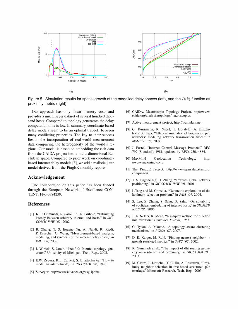
To analyse the growth properties of each delayspace, we performed several experiments each timeincrementing the radius r by one millisecond. Fig. 5(a)depicts our results. The x-axis illustrates the variationof the delay radius r whereas the y-axis shows themedian of all obtained Bp(2r) /Bp(r) samples foreach specific value of r. Regarding the reference

4. It is shown in [2] that the properties we are going to ascertainby our metrics are independent of the sample size. Thus, it does notmatter if we set it to 500 or 3000 nodes.

0

100

200

300

400

500

600

700

800

0 5000 10000 15000 20000

Mea

sure

d ro

und-

trip

time

(in m

sec)

Distance (in kilometres)

Speed of light in fiberLinear regression (world)

(a)

0

20

40

60

80

100

0 50 100 150 200 250 300

Larg

e Cl

uste

r Per

cent

age

Cutoff delay (in msec)

Measured (King)Coordinate-based

AnalyticalInet

GT-ITM

(b)

Figure 4. Results of linear regression with least square analysis on CAIDA measurement data (left).Simulation results for cutoff delay clustering (right).

model, it can be seen that the curves oscillates twotimes having a peak at delay radius values 20 ms and102 ms. Also, our coordinate-based approach and theanalytical function produces these two characteristicpeaks at 26 ms and 80 ms, and 31 ms and 76 msrespectively5.

In all of the three mentioned delay spaces, theincrease of the delay radius firstly covers most ofthe nodes located in each of the three major clusters.Afterwards, the spatial growth decreases as long as ris high enough to cover nodes located in another majorcluster. Then, it increases again until all nodes arecovered, and the curves flatten out. The derived growthconstant for this first peak of the analytical functionis, however, an order of magnitude higher than theconstants of the others. This is clearly a consequence ofour approximation through linear regression. Since thisfunction only represents an average view on the globalRTTs, it cannot predict lifelike delays with regard tothe geographical location of peers. Nevertheless, thisfunction performs better than both topology generateddelay spaces. More precisely, none of both reflectthe growth properties observed by our reference delayspace.

The experiments with the D(k)-metric confirm thetrend of our previous findings. The predicted delaysof our coordinate-based model accurately matches themeasured delays of the reference model. Fig. 5(b)illustrates the simulation results. While varying thenumber of k (x-axis), we plot the delay derived bythe D(k)-function over the average to all-node delay.Whilst especially the measured delays and the one

5. The minimum delay produced by the analytical function is31ms, no matter the distance. This is why there are no values forthe first 30 ms of r.

predicted by our model show the noticeable char-acteristic that there are a few nodes whose delayare significantly smaller than the overall average, thetopology generated delays do not resemble this. As aconsequence, it is likely that the application of PNSmechanisms in reality will lead to highly differentresults when compared to the ones forecasted withGT-ITM or Inet topologies. The analytical function,on the other hand, performs significantly better thanthe topology generators, even though there is also anoticeable difference in the results obtained by formertwo delay spaces.

6. ConclusionSimulation is probably the most important tool for

the validation and performance evaluation of p2p sys-tems. The performance of overlay networks dependsstrongly on a realistic Internet model. Several differentmodels for the simulation of link delays have been pro-posed in the past, which all have severe shortcomings.Most approaches do not incorporate the properties ofthe geographic region of the host. Hosts in a generatedtopology thus have overly uniform delay properties.The analytical approach, on the other hand, does notprovide a jitter modell that reflects the different regionsand the absolute delays differ from more realisticapproaches. Only the King model yields results similarto our coordinate-based system. This proves the real-ism of our approach because King is directly derivedfrom real-world measurements. The major drawbackof King is its limited scalability. It requires memoryproportional to n2 and available datasets are limitedto 3997 measured hosts. Statistical scaling of this dataallows us to preserve delay properties, but producessolely static delay values [2].

1

10

100

0 100 200 300 400 500

Med

ian

B(2r

)/B(r)

Radius r (in msec)

Measured (King)Coordinate-based

AnalyticalInet

GT-ITM

(a)

0

0.2

0.4

0.6

0.8

1

0 0.2 0.4 0.6 0.8 1

D(k)

/D(N

)

k/N

Measured (King)Coordinate-based

AnalyticalInet

GT-ITM

(b)

Figure 5. Simulation results for spatial growth of the modelled delay spaces (left), and the D(k)-function asproximity metric (right).

Our approach has only linear memory costs andprovides a much larger dataset of several hundred thou-sand hosts. Compared to topology generators the delaycomputation time is low. In summary, coordinate-baseddelay models seem to be an optimal tradeoff betweenmany conflicting properties. The key to their successlies in the incorporation of real-world measurementdata comprising the heterogeneity of the world’s re-gions. Our model is based on embedding the rich datafrom the CAIDA project into a multi-dimensional Eu-clidean space. Compared to prior work on coordinate-based Internet delay models [8], we add a realistic jittermodel derived from the PingER monthly reports.

AcknowledgementThe collaboration on this paper has been funded

through the European Network of Excellence CON-TENT, FP6-0384239.

References

[1] K. P. Gummadi, S. Saroiu, S. D. Gribble, “Estimatinglatency between arbitrary internet end hosts,” in SIG-COMM IMW ’02, 2002.

[2] B. Zhang, T. S. Eugene Ng, A. Nandi, R. Riedi,P. Druschel, G. Wang, “Measurement-based analysis,modeling, and synthesis of the internet delay space,” inIMC ’06, 2006.

[3] J. Winick, S. Jamin, “Inet-3.0: Internet topology gen-erator,” University of Michigan, Tech. Rep., 2002.

[4] E.W. Zegura, K.L. Calvert, S. Bhattacharjee, “How tomodel an internetwork,” in INFOCOM ’96, 1996.

[5] Surveyor, http://www.advance.org/csg-ippm/.

[6] CAIDA. Macroscopic Topology Project, http://www.caida.org/analysis/topology/macroscopic/.

[7] Active measurement project, http://watt.nlanr.net.

[8] G. Kunzmann, R. Nagel, T. Hossfeld, A. Binzen-hofer, K. Eger, “Efficient simulation of large-Scale p2pnetworks: modeling network transmission times,” inMSOP2P ’07, 2007.

[9] J. Postel, “Internet Control Message Protocol,” RFC792 (Standard), 1981, updated by RFCs 950, 4884.

[10] MaxMind Geolocation Technology, http://www.maxmind.com/.

[11] The PingER Project, http://www-iepm.slac.stanford.edu/pinger/.

[12] T. S. Eugene Ng, H. Zhang, “Towards global networkpositioning,” in SIGCOMM IMW ’01, 2001.

[13] L.Tang and M. Crovella, “Geometric exploration of thelandmark selection problem,” in PAM ’04, 2004.

[14] S. Lee, Z. Zhang, S. Sahu, D. Saha, “On suitabilityof euclidean embedding of internet hosts,” in SIGMET-RICS ’06, 2006.

[15] J. A. Nelder, R. Mead, “A simplex method for functionminimization,” Computer Journal, 1965.

[16] G. Tyson, A. Mauthe, “A topology aware clusteringmechanism,” in PGNet ’07, 2007.

[17] D. R. Karger, M. Ruhl, “Finding nearest neighbors ingrowth restricted metrics,” in SoTC ’02, 2002.

[18] K. Gummadi et al., “The impact of dht routing geom-etry on resilience and proximity,” in SIGCOMM ’03,2003.

[19] M. Castro, P. Druschel, Y. C. Hu, A. Rowstron, “Prox-imity neighbor selection in tree-based structured p2poverlays,” Microsoft Research, Tech. Rep., 2003.