Modelling the Evolution of Credit Spreads using the Cox Process within the HJM Framework: A CDS Option Pricing Model

Electronic copy available at: http://ssrn.com/abstract=1352114

QUANTITATIVE FINANCE RESEARCH CENTRE

Quantitative Finance Research Centre Research Paper 232 October 2008

Modelling the evolution of Credit Spreads using the Cox Process within the HJM framework: a CDS option pricing model

Carl Chiarella, Viviana Fanelli and Silvana Musti

ISSN 1441-8010

Electronic copy available at: http://ssrn.com/abstract=1352114

Modelling the Evolution of Credit Spreads using theCox process within the HJM framework: a CDS

Option Pricing Model

Carl Chiarella∗ Viviana Fanelli† Silvana Musti‡

Abstract

In this paper a simulation approach for defaultable yield curves is developed withinthe Heath et al. (1992) framework. The default event is modelled using the Cox pro-cess where the stochastic intensity represents the credit spread. The forward creditspread volatility function is affected by the entire credit spread term structure. Thepaper provides the defaultable bond and credit default swap option price in a proba-bility setting equipped with a subfiltration structure. The Euler-Maruyama stochasticintegral approximation and the Monte Carlo method are applied to develop a numer-ical scheme for pricing. Finally, the Antithetic Variable technique is used to reducethe variance of credit default swap option prices.

Keywords: Pricing, HJM model, Cox process, Monte Carlo method, CDS optionJEL Classification: C63, G13, G33

∗School of Finance and Economics, University of Technology, Sydney, PO Box 123, Broadway, NSW2007, Australia ([email protected])

†Corresponding Author: Dipartimento di Scienze Economiche, Matematiche e Statistiche, Universitàdegli Studi di Foggia, Largo Papa Giovanni Paolo II, 1, 71100, Foggia, Italy ([email protected])

‡Dipartimento di Scienze Economiche, Matematiche e Statistiche, Università degli Studi di Foggia,Largo Papa Giovanni Paolo II, 1, 71100, Foggia, Italy ([email protected])

1

1 IntroductionSince the 1990s, the focus on credit risk has increased amongst academics and financialmarket practitioners. This is due to the concerns of regulatory agencies and investorsregarding the high exposure of financial institutions to over-the-counter derivatives. Itis also due to the rapid development of markets for price-sensitive and credit-sensitiveinstruments that allow institutions and investors to trade this risk.

The New Basel Accord (International Convergence of Capital Measurement and CapitalStandard, Basel II, 26 January 2004) promotes the standards for credit risk management,obligating financial institutions to fulfill a variety of regulatory capital requirements. Byincreasing the reliability of the credit derivative market, the Basel II rules have contributedto its success.

In the credit risk literature two principal kinds of models are widely used: the structuralmodels and the reduced form models.

Structural models were proposed by Merton (1974), Black and Cox (1976), Shimkoet al. (1993) and Longstaff and Schwartz (1995), to cite the principal contributions. Thesemodels focus on the analysis of a firm’s structural variables: the default event derives fromthe evolution of the firm’s assets and it is completely specified in an endogenous way.

The main drawback of the structural approach is that since many of the firm’s assetsare typically not traded, the firm’s value process is fundamentally unobservable, makingimplementation difficult. Furthermore, this approach assumes that only bonds with ho-mogeneous levels of seniority exist and that the risk-free rates are constant over the periodof evaluation.

Zhou (1997) and Schönbucher (1996) are two important contributions that use jumpdiffusion processes for the evolution of the firm’s value in the Merton model. These modelsare more realistic in generating the shape of a credit spread term structure compared to theclassical structural models that seem to underestimate credit spread values. Jump-diffusionmodels also have the advantage of allowing the default event to occur abruptly.

Reduced form models are characterized by a more flexible approach to credit risk.They mainly model the spread between the defaultable interest rate and the risk-free rate.The default time is a stochastic variable modelled as a stopping time. The two earliestcontributions to this approach are those of Jarrow and Turnbull (1995) and Jarrow et al.(1997).

Jarrow and Turnbull (1995) consider a constant and deterministic Poisson intensity.In contrast, Jarrow et al. (1997) consider the issuer’s rating as the fundamental variabledriving the default process and the rating dynamics are modelled as a Markov chain, wheredefault is the absorbing state.

Lando (1998) uses a stochastic intensity, while the default process is described by aCox process which allows a remarkable degree of analytical tractability. The Cox processis a generalization of the Poisson process when the intensity is random. If the Cox processis conditional on a particular realization of the intensity, it becomes an inhomogeneousPoisson process.

Das and Sundaram (2000) find a more flexible pricing methodology valid both for bondsand credit derivatives. A defaultable bond price is equal to the expected value of futurepayoffs discounted by a defaultable interest rate. The term structure models existing inthe literature, such as Cox et al. (1985) and Heath et al. (1992) can then be used to model

2

the defaultable term structure.An important result demonstrated in Duffie and Lando (2001) is the way in which a

structural model of the Black and Cox (1976) type is consistent with the reduced formclass of models when asymmetric information about structural characteristics is revealed.

Recently, academics and practitioners have utilized the risk-neutral pricing methodol-ogy to carry out credit spread term structure analysis. Duffie and Singleton (1999) providea discrete-time reduced-form model in order to evaluate risky debt and credit derivatives inan arbitrage-free environment. They add a forward spread process to the forward risk-freerate process and use the Heath et al. (1992) approach to obtain the arbitrage-free driftrestriction and by using the "Recovery of Market Value" condition (Duffie and Singleton(1999)), they provide a recursive formula that is easy to implement.

The HJM approach is used by Schönbucher (1998) in order to model the term structureof defaultable interest rates. The defaultable bond price is obtained under the followingassumptions: i) positive recovery rates, ii) reorganization of the defaulted firms with thepossibility of multiple default, and iii) uncertainty about the magnitude of the default.Furthermore, the firm’s default causes jumps in the defaultable interest rate process. Usingthe HJM approach, Schönbucher (1998) provides a drift restriction for the defaultableterm structure. A similar result is obtained in Pugachevsky (1999), where the HJM driftrestriction is obtained by applying the arbitrage free condition obtained in Maksyumiukand Gatarek (1999) and without assuming any jumps to default.

Finally, Jeanblanc and Rutkowski (2002), Jamshidian (2004) and Brigo and Morini(2005) suggest a different approach to defaultable bond and credit derivative modelling:in a probability space equipped with a subfiltration structure the default is modelled as aCox process. Furthermore, Chen et al. (2008) provide a model for valuing a credit defaultswap when the interest rate and the hazard rate are correlated. They provide an explicitsolution to the model by solving a bivariate Riccati equation. Their model is solved quicklyso that all the parameters of the model are simultaneously estimated.

In this paper, we build on the cited recent literature and develop a model for creditspread term structure evolution and credit derivative pricing. The HJM model has beenextensively analyzed in the literature from a theoretical point of view: our intent, instead, isto focus on the applications of the model for pricing purposes. In particular, we model theforward credit spread curve within the HJM framework using the theory of Cox processeswhere the stochastic intensity represents the credit spread. The HJM model is known tobe one of the most general term structure models and for this reason we have chosen toextend its interest rate dynamics to the defaultable rate: the forward credit spread volatilityfunction, the initial credit spread curve and specifications of the volatility structure are thesole inputs. Because of the arbitrage-free condition, the drift can be expressed in terms ofthe volatility. We assume a stochastic volatility for both the risk-free interest rate and thecredit spread, so that analytical results are not readily available and model implementationis generally possible only via a numerical simulation approach. We develop and implementan efficient numerical scheme that allows bond and credit derivative pricing. The accuracyof the calculated values is improved by the application of a well known method of variancereduction, the Antithetic Variable technique.

In Section 2 we describe the model. In Section 3 we outline the foundations of creditdefault swap (CDS) pricing and derive CDS option pricing formulae under the equivalentmartingale measure. In Section 4 we outline the application of Monte Carlo simulation to

3

the HJM model based on the Euler-Maruyama discretisation of the forward rate dynamics.A variance reduction technique is applied to improve the efficiency of the Monte Carlomethod and to provide more accurate numerical results for pricing. Then, the efficiency ofthe computational technique in terms of runtimes is investigated. The analysis concerningthe runtime/accuracy trade-off indicates how the evaluation method can be successfullyutilized by credit risk practitioners who wish to price credit risk products with satisfactorylevels of accuracy and reasonable runtimes. Section 5 concludes.

2 Model settingThe model is set in a filtered probability space (Ω,F , (Ft)t≥0,P), T is assumed to be thefinite time horizon and F = FT is the σ-algebra at time T . All statements and definitionsare understood to be valid until the time horizon T . The probability space is assumed to belarge enough to support both an Rd-valued stochastic process X = Xt : 0 ≤ t ≤ T thatis right continuous with left limit, and a Poisson process N(t) with N(0) = 0, independentof X.

The background driving process X generates the subfiltration H = (Ht)t≥0 = (σ(Xs :0 ≤ s ≤ t))t≥0 representing the flow of all background information except default itself andH = HT is the sub-σ-algebra at time T .

The Poisson process N(t) has a non negative and right-continuous stochastic intensityλ(t) which is independent of N(t) and follows the diffusion process

dλ(t) = µλ(t)dt + σλ(t)dWλ(t), (1)

where µλ(t) is the drift of the intensity process, σλ(t) is the volatility of the intensityprocess and Wλ is a standard Wiener process under the objective probability measure P.The intensity process λ(t) is assumed to be adapted to H, and the assumption of timedependent intensity implies the existence of an inhomogeneous Poisson process.

In the subfiltration setting outlined above it is natural to consider an Ht-conditionalPoisson process in such a way that a Cox process is associated with the state variablesprocess X and the intensity function λ(t). We define τi, i ∈ N, as the times of defaultgenerated by the Cox process N(t) =

∑∞i=1 1τi≤t with intensity λ(t). We only consider

the time of the first default and it will be referred to with τ := τ1. Then, the defaultabletime τ is a stopping time, τ : Ω → R+

0 , defined as the first jump time of N(t),

τ = inft ∈ R+0 |N(t) > 0.

The right-continuous default indicator process 1τ≤t generates the subfiltration Fτ =(F τ

t )t≥0 = (σ(1τ≤s : 0 ≤ s ≤ t))t≥0, that is assumed to be one component of the fullfiltration F = (Ft)t≥0. Since obviously F τ

t ⊂ Ft, ∀t ∈ R+0 , τ is a stopping time with

respect to F, but it is not necessarily a stopping time with respect to H. It follows thatF = H ∨ Fτ , that is Ft = Ht ∨ F τ

t ∀t ∈ R+0 .

For any t ∈ R+0 , we define the default probability as P(τ ≤ t|Ht) and the survival

probability as P(τ > t|Ht). These two quantities indicate, respectively, the probability ofdefault occurring or not occurring up to time t. In the subfiltration setting, asset pricingis consistent with the application of the iterated expectation law.

4

At any time t, the risk-free zero-coupon bond price is denoted by P (t, T ), where Trepresents the maturity time, T > t, and it is calculated according to

P (t, T ) = e−R T

t f(t,s)ds, (2)

where f(t, T ) is the instantaneous risk free forward rate at time t applicable at fixedmaturity T . Conversely, if the derivative of P (t, T ) with respect to maturity T exists, theinstantaneous risk free forward rate can be written in terms of the bond price as

f(t, T ) = − ∂

∂TlogP (t, T ). (3)

We assume that the forward rate is driven by the diffusion process

df(t, T ) = α(t, T, ·)dt + σ(t, T, ·)dW (t), (4)

where α(t, T, ·) is the instantaneous forward rate drift function, σ(t, T, ·) is the instanta-neous forward rate volatility function and W (t) is a standard Wiener process with respectto the objective probability measure P. The third argument in the brackets (t, T, ·) indi-cates the possible forward rate dependence on other path dependent quantities, such as thespot rate or the forward rate itself. The instantaneous risk-free short rate r(t) is definedas r(t) := f(t, t).We recall that the HJM no-arbitrage drift restriction is

α(t, T, ·) = σ(t, T, ·)[∫ T

t

σ(t, s, ·)ds− φ(t)

]. (5)

Similar statements hold for defaultable bonds. We indicate with Pd,R(t, T ) the genericprice at any time t of a defaultable zero-coupon bond with maturity T and recovery rateR. If we set

Pd(t, T ) := Pd,0(t, T ),

we havePd(t, T ) = 1τ>te

− R Tt fd(t,s)ds, (6)

where fd(t, T ) is the instantaneous defaultable forward rate at time t applicable to fixedmaturity T . If the derivative of Pd(t, T ) with respect to maturity T exists and assumingthat the default occurs after t, the instantaneous defaultable forward rate can be writtenin terms of the bond price as

fd(t, T ) = − ∂

∂TlogPd(t, T ) (7)

and is assumed to be modelled by the stochastic process

dfd(t, T ) = αd(t, T, ·)dt + σd(t, T, ·)dWd(t), (8)

where αd(t, T, ·) and σd(t, T, ·) are, respectively, the drift function and the volatility func-tion of the instantaneous defaultable forward rate. Furthermore Wd(t) is a standard Wienerprocess with respect to the objective probability measure P. As in (4), the third argumentin the brackets (t, T, ·) indicates, again, the possible defaultable forward rate dependence

5

on other path dependent quantities, such as the defaultable spot rate or the defaultableforward rate itself.

Spot rate dynamics are derived from the forward rate dynamics, since rd(t) := fd(t, t).Recalling that the market is arbitrage free if and only if there exists a probability measureP such that discounted asset price processes are martingales, the defaultable bond price isnow obtained as the risk-neutral expectation of the discounted bond value, namely

Pd(t, T ) = 1τ>tEeP[e−R T

t rd(s)ds|Ht] (9)

where e−R T

t rd(s)ds is the defaultable stochastic discount factor and P is the risk-neutralequivalent probability measure.

Following Lando (1998), the pricing formula at time t for a defaultable zero couponbond with maturity T is given by

Pd(t, T ) = EeP[e−R T

t r(s)ds1τ>T|Ft] =

= EeP[EeP[e−R T

t r(s)ds1τ>T|HT ∨ F τt ]|Ft] =

= EeP[e−R T

t r(s)ds1τ>tEeP[1τ>T|HT ∨ F τt ]|Ft] =

= 1τ>tEeP[e−R T

t (r(s)+λ(s))ds|Ft] =

= 1τ>tEeP[e−R T

t (r(s)+λ(s))ds|Ht]. (10)

The last equation follows from the law of iterated expectations. Comparing equation (9)with equation (10), we see that the default free and defaultable instantaneous spot rateare related by

rd(t) = r(t) + λ(t), (11)

where λ(t) is the (stochastic) intensity rate. So the credit spread at the short end is λ(t).Equation (11) suggests writing the credit spread across rates of all maturities as λs(t, T )so that

fd(t, T ) = f(t, T ) + λs(t, T ). (12)

We assume for λs(t, T ) the dynamics

λs(t, T ) = λs(0, T ) +

∫ t

0

αλ(s, T, ·)ds +

∫ t

0

σλ(s, T, ·)dWλ(s), (13)

where αλ(t, T, ·) is the drift, σλ(t, T, ·) is the volatility of the credit spread curves and Wλ(t)is a standard Wiener process under P. For (11) and (12) to be compatible at T = t wemust have

λ(t) = λs(t, t). (14)

From (13) it follows that the stochastic integral equation for λ(t) may be written

λ(t) = λs(t, t) = λs(0, t) +

∫ t

0

αλ(s, t, ·)ds +

∫ t

0

σλ(s, t, ·)dWλ(s), (15)

from which (the subscript 2 denotes partial derivative with respect to the second argument)

dλ(t) =

[αλ(t, t, ·) +

∫ t

0

αλ2(s, t, ·)ds +

∫ t

0

σλ2(s, t, ·)dWλ(s)

]dt +

σλ(t, t, ·)dWλ(t). (16)

6

Thus in order that (1) and (16) be compatible it must be the case that the µλ(t) and σλ(t)in equation (1) are given by

µλ(t) = αλ(t, t, ·) +

∫ t

0

αλ2(s, t, ·)ds +

∫ t

0

σλ2(s, t, ·)dWλ(s),

σλ(t) = σλ(t, t, ·).

For simplicity of expression we shall assume stochastic differential equations driven by oneBrownian motion for both the risk-free forward rate and the credit spread. Consequently,the correlation between the Brownian motions dW and dWλ becomes a scalar coefficientthat we write as

ρ = corr(dW, dWλ). (17)

We use the Heath et al. (1992) approach to model the term structure of defaultableinterest rates. The main advantages of the HJM model are that in the formulation of thespot rate process and bond price process the market price of interest rate risk drops outby being incorporated into the Wiener process under the risk neutral measure; the modelis automatically calibrated to the initial yield curve and the drift term in the forward ratedifferential equation is a function of the volatility term. As result of the latter characteristic,the HJM model can be considered as a class of models, each one identified by the choice of avolatility function. Consequently, we need to give a specific functional form to the volatilityterm in order to obtain a specific HJM model. The main complication of this approachis that some volatility functions make the dynamics for r(t) and rd(t) path dependent,in other words non-Markovian, and since the bond price dynamics depend on these, theyalso become non-Markovian making the model difficult to handle, both analytically andnumerically.

Using the HJM approach, we show in Appendix B that the no-arbitrage restriction onthe drift of the credit spread process may be written as

αλ(t, T ) =ρ

[σ(t, T )

∫ T

t

σλ(t, s)ds + σλ(t, T )

∫ T

t

σ(t, s)ds

]dv

+ σλ(t, T )

∫ T

t

σλ(t, s)ds− σλ(t, T )φλ(t).

so that the stochastic dynamics for the defaultable forward rate, written in integral form,are

fd(t, T ) = f(0, T ) + λs(0, T )

+∫ t

0

[σ(v, T )

∫ T

vσ(v, s)ds + σλ(v, T )

∫ T

vσλ(v, s)ds

]dv

+∫ t

0ρ

[σ(v, T )

∫ T

vσλ(v, s)ds + σλ(v, T )

∫ T

vσ(v, s)ds

]dv

+∫ t

0

[σ(v, T )dW (v) + σλ(v, T )dWλ(v)

]. (18)

7

In (18)

W (t) = W (t)−∫ t

0

φ(s)ds, (19)

Wλ(t) = Wλ(t)−∫ t

0

φλ(s)ds, (20)

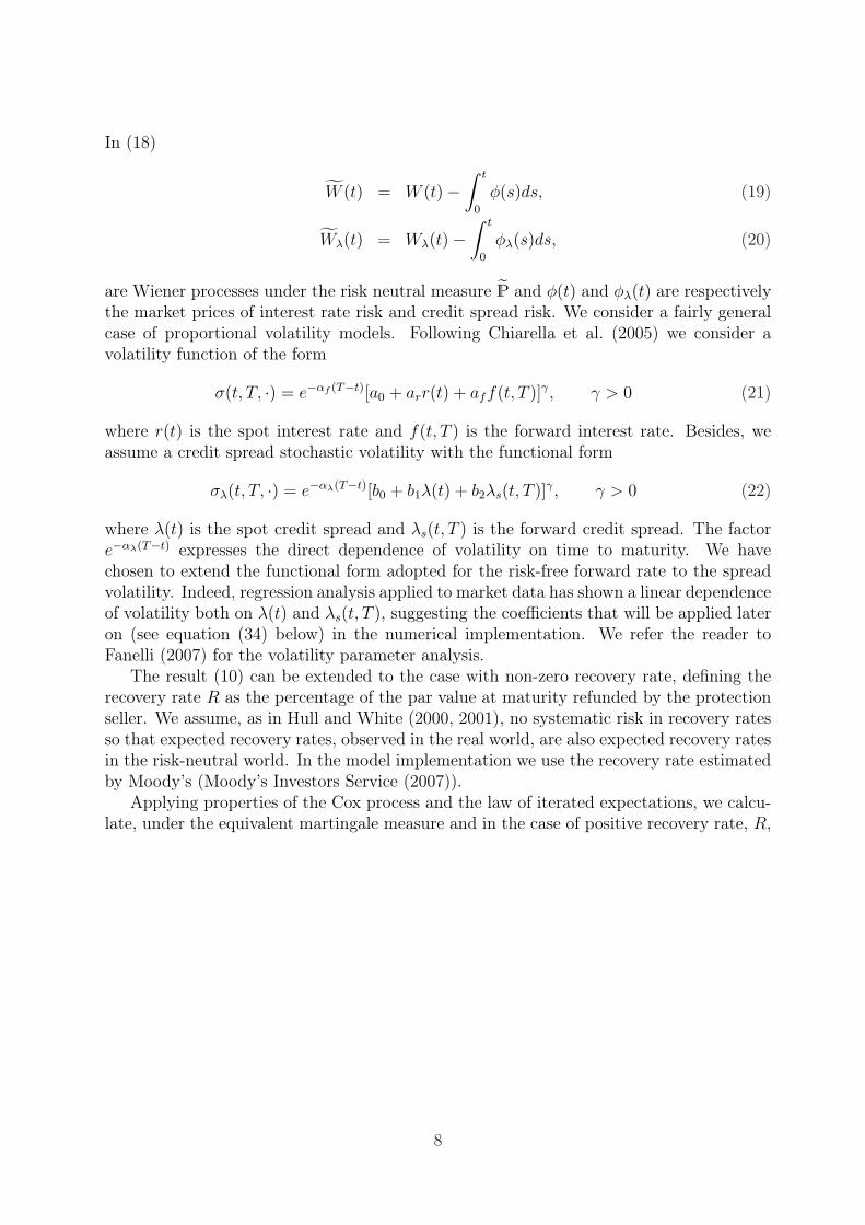
are Wiener processes under the risk neutral measure P and φ(t) and φλ(t) are respectivelythe market prices of interest rate risk and credit spread risk. We consider a fairly generalcase of proportional volatility models. Following Chiarella et al. (2005) we consider avolatility function of the form

σ(t, T, ·) = e−αf (T−t)[a0 + arr(t) + aff(t, T )]γ, γ > 0 (21)

where r(t) is the spot interest rate and f(t, T ) is the forward interest rate. Besides, weassume a credit spread stochastic volatility with the functional form

σλ(t, T, ·) = e−αλ(T−t)[b0 + b1λ(t) + b2λs(t, T )]γ, γ > 0 (22)

where λ(t) is the spot credit spread and λs(t, T ) is the forward credit spread. The factore−αλ(T−t) expresses the direct dependence of volatility on time to maturity. We havechosen to extend the functional form adopted for the risk-free forward rate to the spreadvolatility. Indeed, regression analysis applied to market data has shown a linear dependenceof volatility both on λ(t) and λs(t, T ), suggesting the coefficients that will be applied lateron (see equation (34) below) in the numerical implementation. We refer the reader toFanelli (2007) for the volatility parameter analysis.

The result (10) can be extended to the case with non-zero recovery rate, defining therecovery rate R as the percentage of the par value at maturity refunded by the protectionseller. We assume, as in Hull and White (2000, 2001), no systematic risk in recovery ratesso that expected recovery rates, observed in the real world, are also expected recovery ratesin the risk-neutral world. In the model implementation we use the recovery rate estimatedby Moody’s (Moody’s Investors Service (2007)).

Applying properties of the Cox process and the law of iterated expectations, we calcu-late, under the equivalent martingale measure and in the case of positive recovery rate, R,

8

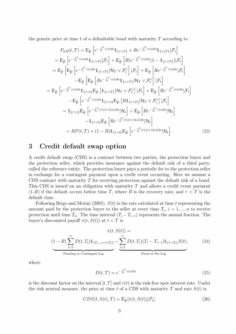
the generic price at time t of a defaultable bond with maturity T according to

Pd,R(t, T ) = EeP[e−

R Tt r(s)ds1τ>T + Re−

R Tt r(s)ds1τ≤T|Ft

]

= EeP[e−

R Tt r(s)ds1τ>T|Ft

]+ EeP

[R(e−

R Tt r(s)ds(1− 1τ>T)|Ft

]

= EeP[EeP

[e−

R Tt r(s)ds1τ>T|HT ∨ F τ

t

]|Ft

]+ EeP

[Re−

R Tt r(s)ds|Ft

]

−EeP[EeP

[Re−

R Tt r(s)ds1τ>T|HT ∨ F τ

t

]|Ft

]

= EeP[e−

R Tt r(s)ds1τ>tEeP

[1τ>T|HT ∨ F τ

t

] |Ft

]+ EeP

[Re−

R Tt r(s)ds|Ft

]

−EeP[e−

R Tt r(s)ds1τ>tEeP

[R1τ>T|HT ∨ F τ

t

] |Ft

]

= 1τ>tEeP[e−

R Tt (r(s)+λ(s))ds|Ht

]+ EeP

[Re−

R Tt r(s)ds|Ht

]

−1τ>tEeP[Re−

R Tt (r(s)+λ(s))ds|Ht

]

= RP (t, T ) + (1−R)1τ>tEeP[e−

R Tt (r(s)+λ(s))ds|Ht

]. (23)

3 Credit default swap optionA credit default swap (CDS) is a contract between two parties, the protection buyer andthe protection seller, which provides insurance against the default risk of a third party,called the reference entity. The protection buyer pays a periodic fee to the protection sellerin exchange for a contingent payment upon a credit event occurring. Here we assume aCDS contract with maturity T for receiving protection against the default risk of a bond.This CDS is issued on an obligation with maturity T and allows a credit event payment(1-R) if the default occurs before time T , where R is the recovery rate, and τ < T is thedefault time.

Following Brigo and Morini (2005), S(t) is the rate calculated at time t representing theamount paid by the protection buyer to the seller at every time Ti, i = 1, ..., n to receiveprotection until time Tn. The time interval (Ti−Ti−1) represents the annual fraction. Thebuyer’s discounted payoff π(t, S(t)) at t < T is

π(t, S(t)) =

(1−R)n∑

i=1

D(t, Ti)1Ti−1<τ≤Ti

︸ ︷︷ ︸Floating or Contingent Leg

−n∑

i=1

D(t, Ti)(Ti − Ti−1)1τ>TiS(t)

︸ ︷︷ ︸Fixed or Fee Leg

, (24)

where

D(t, T ) = e−R T

t r(s)ds (25)

is the discount factor on the interval [t, T ] and r(t) is the risk-free spot interest rate. Underthe risk neutral measure, the price at time t of a CDS with maturity T and rate S(t) is

CDS(t, S(t), T ) = EeP[π(t, S(t))|Ft]. (26)

9

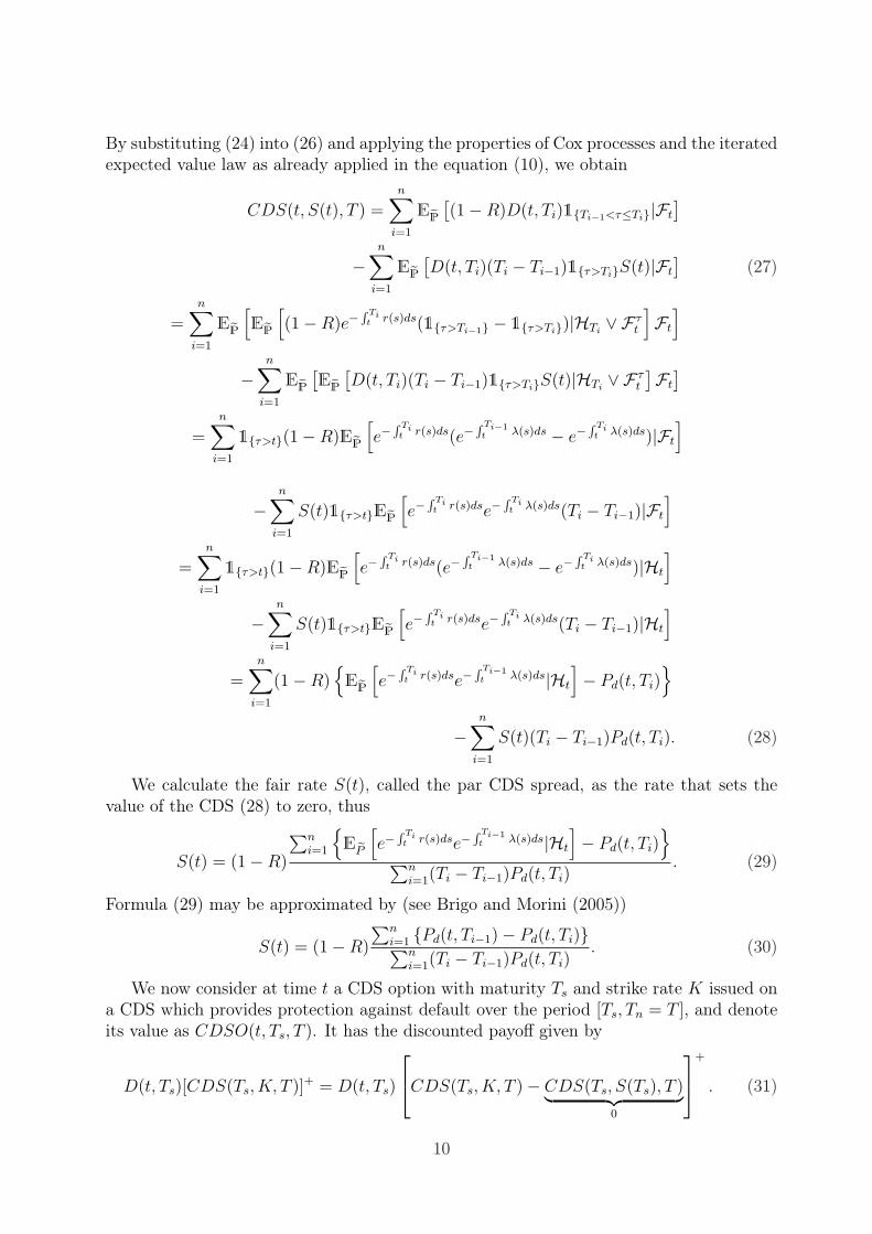
By substituting (24) into (26) and applying the properties of Cox processes and the iteratedexpected value law as already applied in the equation (10), we obtain

CDS(t, S(t), T ) =n∑

i=1

EeP[(1−R)D(t, Ti)1Ti−1<τ≤Ti|Ft

]

−n∑

i=1

EeP[D(t, Ti)(Ti − Ti−1)1τ>TiS(t)|Ft

](27)

=n∑

i=1

EeP[EeP

[(1−R)e−

R Tit r(s)ds(1τ>Ti−1 − 1τ>Ti)|HTi

∨ F τt

]Ft

]

−n∑

i=1

EeP[EeP

[D(t, Ti)(Ti − Ti−1)1τ>TiS(t)|HTi

∨ F τt

]Ft

]

=n∑

i=1

1τ>t(1−R)EeP[e−

R Tit r(s)ds(e−

R Ti−1t λ(s)ds − e−

R Tit λ(s)ds)|Ft

]

−n∑

i=1

S(t)1τ>tEeP[e−

R Tit r(s)dse−

R Tit λ(s)ds(Ti − Ti−1)|Ft

]

=n∑

i=1

1τ>t(1−R)EeP[e−

R Tit r(s)ds(e−

R Ti−1t λ(s)ds − e−

R Tit λ(s)ds)|Ht

]

−n∑

i=1

S(t)1τ>tEeP[e−

R Tit r(s)dse−

R Tit λ(s)ds(Ti − Ti−1)|Ht

]

=n∑

i=1

(1−R)EeP

[e−

R Tit r(s)dse−

R Ti−1t λ(s)ds|Ht

]− Pd(t, Ti)

−n∑

i=1

S(t)(Ti − Ti−1)Pd(t, Ti). (28)

We calculate the fair rate S(t), called the par CDS spread, as the rate that sets thevalue of the CDS (28) to zero, thus

S(t) = (1−R)

∑ni=1

E eP

[e−

R Tit r(s)dse−

R Ti−1t λ(s)ds|Ht

]− Pd(t, Ti)

∑n

i=1(Ti − Ti−1)Pd(t, Ti). (29)

Formula (29) may be approximated by (see Brigo and Morini (2005))

S(t) = (1−R)

∑ni=1 Pd(t, Ti−1)− Pd(t, Ti)∑n

i=1(Ti − Ti−1)Pd(t, Ti). (30)

We now consider at time t a CDS option with maturity Ts and strike rate K issued ona CDS which provides protection against default over the period [Ts, Tn = T ], and denoteits value as CDSO(t, Ts, T ). It has the discounted payoff given by

D(t, Ts)[CDS(Ts, K, T )]+ = D(t, Ts)

CDS(Ts, K, T )− CDS(Ts, S(Ts), T )︸ ︷︷ ︸

0

+

. (31)

10

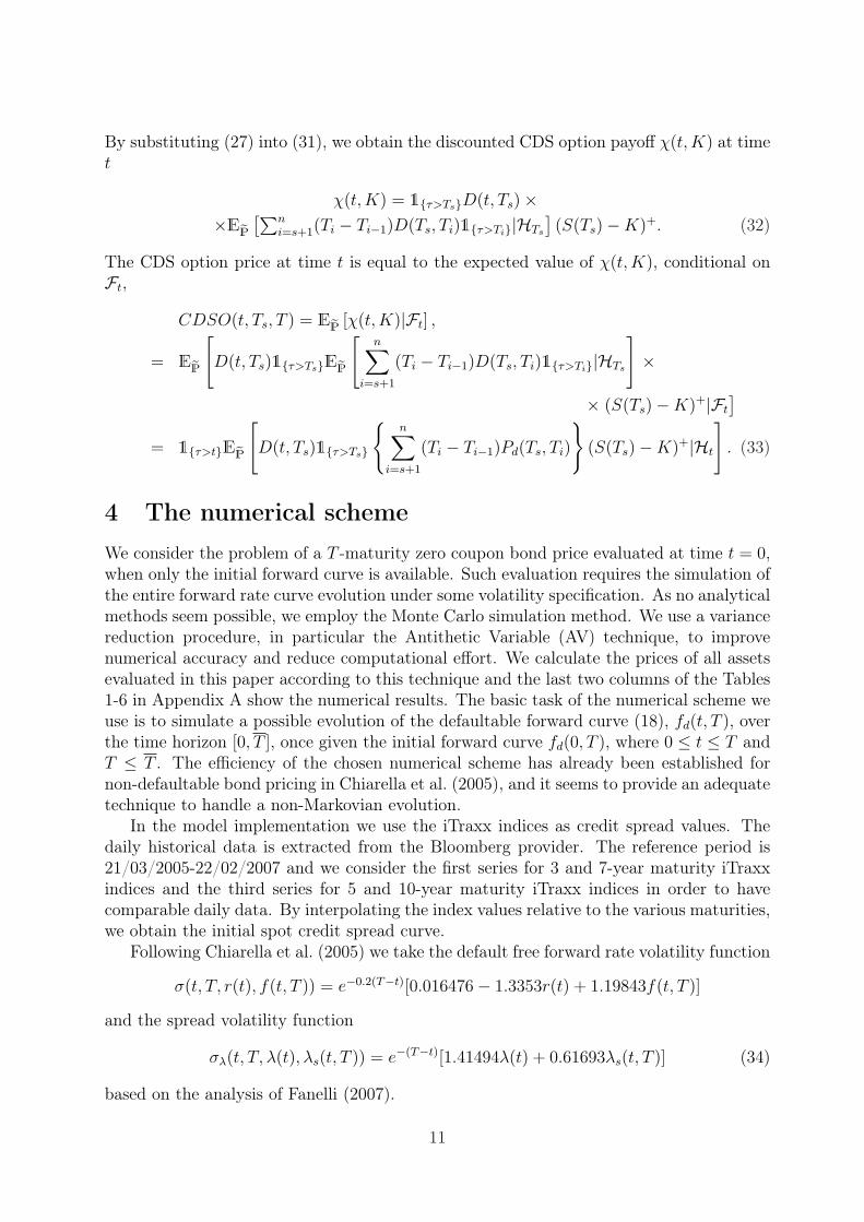
By substituting (27) into (31), we obtain the discounted CDS option payoff χ(t,K) at timet

χ(t,K) = 1τ>TsD(t, Ts)××EeP

[∑ni=s+1(Ti − Ti−1)D(Ts, Ti)1τ>Ti|HTs

](S(Ts)−K)+. (32)

The CDS option price at time t is equal to the expected value of χ(t,K), conditional onFt,

CDSO(t, Ts, T ) = EeP [χ(t,K)|Ft] ,

= EeP

[D(t, Ts)1τ>TsEeP

[n∑

i=s+1

(Ti − Ti−1)D(Ts, Ti)1τ>Ti|HTs

]×

× (S(Ts)−K)+|Ft

]

= 1τ>tEeP

[D(t, Ts)1τ>Ts

n∑

i=s+1

(Ti − Ti−1)Pd(Ts, Ti)

(S(Ts)−K)+|Ht

]. (33)

4 The numerical schemeWe consider the problem of a T -maturity zero coupon bond price evaluated at time t = 0,when only the initial forward curve is available. Such evaluation requires the simulation ofthe entire forward rate curve evolution under some volatility specification. As no analyticalmethods seem possible, we employ the Monte Carlo simulation method. We use a variancereduction procedure, in particular the Antithetic Variable (AV) technique, to improvenumerical accuracy and reduce computational effort. We calculate the prices of all assetsevaluated in this paper according to this technique and the last two columns of the Tables1-6 in Appendix A show the numerical results. The basic task of the numerical scheme weuse is to simulate a possible evolution of the defaultable forward curve (18), fd(t, T ), overthe time horizon [0, T ], once given the initial forward curve fd(0, T ), where 0 ≤ t ≤ T andT ≤ T . The efficiency of the chosen numerical scheme has already been established fornon-defaultable bond pricing in Chiarella et al. (2005), and it seems to provide an adequatetechnique to handle a non-Markovian evolution.

In the model implementation we use the iTraxx indices as credit spread values. Thedaily historical data is extracted from the Bloomberg provider. The reference period is21/03/2005-22/02/2007 and we consider the first series for 3 and 7-year maturity iTraxxindices and the third series for 5 and 10-year maturity iTraxx indices in order to havecomparable daily data. By interpolating the index values relative to the various maturities,we obtain the initial spot credit spread curve.

Following Chiarella et al. (2005) we take the default free forward rate volatility function

σ(t, T, r(t), f(t, T )) = e−0.2(T−t)[0.016476− 1.3353r(t) + 1.19843f(t, T )]

and the spread volatility function

σλ(t, T, λ(t), λs(t, T )) = e−(T−t)[1.41494λ(t) + 0.61693λs(t, T )] (34)

based on the analysis of Fanelli (2007).

11

We divide [0, T ] into N subintervals of length 4t = TN, so that n = t

4t, m = T

4tfor

0 ≤ t ≤ T ≤ T and f(t, T ) = f(n∆t,m∆t). The Euler-Maruyama discretisation is usedto approximate the stochastic integral equation (18) (see Kloeden and Platen (1999)).

We start by considering at time zero the initial defaultable forward curve with genericmaturity T = m∆t, where 1 ≤ m ≤ N , that is fd(0, 0) = rd(0), fd(0, ∆t), fd(0, 2∆t),..., fd(0, N∆t). Hence we obtain the generic recursive formula for the defaultable forwardcurve evolution in the form

fd((n + 1)∆t,m∆t) = f(n∆t,m∆t) + λ(n∆t, m∆t, ·)+σ(n∆t,m∆t, ·) ∑m−1

i=n σ(n∆t, i∆t, ·)∆t + σλ(n∆t, m∆t, ·) ∑m−1i=n σλ(n∆t, i∆t, ·)∆t

+ρ[σ(n∆t,m∆t, ·) ∑m−1

i=n σλ(n∆t, i∆t, ·)∆t + σλ(n∆t,m∆t, ·) ∑m−1i=n σ(n∆t, i∆t, ·)∆t

]

+σ(n∆t,m∆t, ·)∆W (n + 1) + σλ(n∆t,m∆t, ·)∆Wλ(n + 1). (35)

The numerical scheme is used to price zero coupon defaultable bonds using equation(10), or equation (23) if there is a non-zero recovery rate. We test the accuracy of theevaluation technique by comparing the estimates with the analytical bond price at time 0calculated according to the exact formula

Pd(0, T ) = e−R T0 fd(0,s)ds,

where fd(0, t) is the observed initial defaultable forward curve.Thus we calculate the k− th bond price (k = 0, 1, 2, ..., Π) corresponding to the k− th

simulated path according to

P kd (0, N∆t) = e−

PN−1j=0 [rk(j∆t)+λk(j∆t)]∆t, (36)

where each simulated forward curve also determines the evolution of the spot rate overthe maturity period [0, T ] by setting m = n + 1 in (35). Simulations are repeated over

∏paths and the approximate defaultable bond price value at time zero is given by

PMCd (0, N∆t) =

1∏Q

∑i=0

P id(0, N∆t). (37)

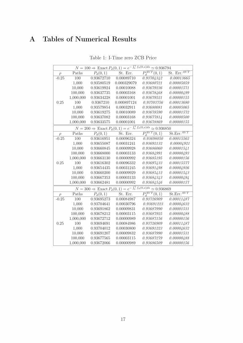
The numerical results for the simulations of time zero bond prices with one year ma-turity are displayed in Table 1. Here and in all the Tables we use the Antithetic Variabletechnique in order to improve numerical accuracy and reduce computational effort. InTable 1 the third and fourth columns refer to the results obtained with the plain MonteCarlo Algorithm, while the last two columns are obtained with the Antithetic Variabletechnique. For each discretisation (N = 100, 200, 300) the exact defaultable bond pricesare calculated and can be compared in Table 1 to the simulated bond prices obtained byvarying the number of paths and the correlation coefficient. This comparison gives us onetest of the efficiency of the numerical scheme and verifies the accuracy of the computations.In Table 1 we illustrate the impact on the standard error of variations of N and Π. Inparticular, in the case of one million paths, the standard error becomes significant at onlythe fifth decimal place. We use both negative and positive correlation values, even thoughthe negative correlation is more consistent with the observed market situation.

12

In the case of positive recovery rate, the value P kd,R(0, N∆t) is approximated by

P kd,R(0, T ) = R e−

PN−1j=0 rk(j∆t)∆t + (1−R)e−

PN−1j=0 [rk(j∆t)+λk(j∆t)]∆t, (38)

and again the Monte Carlo bond price may be computed. Table 2 shows the simulatedinitial price of a bond maturing in one year using Π = 100/1, 000/10, 000 respectively, usingrecovery rates observed in the market (see Moody’s Investors Service (2007)) and N =200. In this case we assume only negative correlation. Also in this case we can comparesimulated results with the actual ones and independently of the recovery rate value, themethod reaches an accuracy of almost four decimal figures after 10,000 simulated paths.PAV T

d and St. ERR.AV T represent respectively the evaluation using the Antithetic Variabletechnique and its standard error. The reduction in the standard errors demonstrates theeffectiveness of this technique.

We now consider the general case in which we evaluate at time t0, 0 ≤ t0 ≤ T ≤ T , adefaultable bond with maturity T and zero recovery rate. We simulate the evolution of thefunction f(t, τ), τ ≥ t, τ ∈ [0, T ], with t varying in [0, t0]. For every t ∈ [0, t0] we obtaintherefore an approximation to the curve f(t, τ), τ ≥ t. We simulate

∏evolutions of the

curve and for the k − th simulated curve at time t0, we calculate the corresponding bondvalue

P kd (t0, T ) = e

− R Tt0

fkd (t0,s)ds

.

Then, the futures price, evaluated at 0, of a bond with delivery t0 and maturity T , thatwe denote Pd(0, t0, T ), is calculated according to

Pd(0, t0, T ) = EeP[Pd(t0, T )|F0],

which can be approximated by the Monte Carlo method as

PMCd (0, t0, T ) =

1∏Q

∑

k=1

P kd (t0, T ) ' EeP[Pd(t0, T )|F0].

For these calculations we simply use the Euler-Maruyama integral approximation

∫ T

t0

fkd (t0, s)ds =

N−1∑i=n

fkd (n∆t, i∆t)∆t.

The numerical results are shown in Table 3. We calculate the value of a zero coupon bondwith 5-year maturity at time t = 2 and of a zero coupon bond with 10-year maturity at timet = 5. The effect of different combinations of (N, Π) on the standard error is shown andthe best accuracy is obtained with N = 500, Π = 10, 000. More accurate approximationsare obtained in the sixth column by applying the AV technique.

Turning now to the credit default swap, we assume at time t the purchase of a CDS ona defaultable zero coupon bond with maturity T and recovery rate R. The contract givesprotection against a default event occurring at time τ over the single interval [Tk−1, Tk],where we recall that Tk = k∆t, Tk−1 = (k − 1)∆t and T = N∆t.

13

Using the Monte Carlo simulation approach above we obtain the approximate fair rateS(0) at time zero as

SMC(0) = (1−R)PMC

d (0, (k − 1)∆t)− PMCd (0, k∆t)

(k∆t− (k − 1)∆t)PMCd (0, k∆t)

. (39)

In Table 4 we display numerical results for a credit default swap contract on a riskyzero coupon bond with recovery rate 0.30 and maturity 3 years, denoted Pd,0.3(0, 3) andwe take N = 300. The protection buyer pays a fee S(0) in exchange for protection againsta default occurring at time τ over the interval [0, 1]. In the first row of the table, the exactCDS rate, calculated using formula (30), is displayed. The accuracy of the approximationimproves by increasing the number of paths. The standard error is significant at the fourthdecimal place. The fourth and fifth columns display the results obtained with the variancereduction technique.

Finally, we consider the credit default swap option. To price this we need to evaluateat time zero a call option with maturity Ts, 0 < Ts < T , issued on a CDS. Under theterms of the CDS, the protection buyer pays a fixed fee K in exchange for a contingentpayment (1−R) upon a credit event occurring over the period [Ts, T ]. The CDSO value isequal to the expected value of the discounted payoff at maturity date with respect to therisk-neutral measure P, namely (see equation (33))

CDSO(0, Ts, T ) =

1τ>0EeP[Pd(0, Ts)

(T − Ts)Pd(Ts, T )

(S(Ts)−K)+|H0

]. (40)

In the numerical scheme the option maturity times are Ts = n∆t and T = N∆t and theMonte Carlo price is given as

CDSOMC(0, n∆t, N∆t) =1∏

Q∑

k=1

CSDOk(0, n∆t, N∆t), (41)

where

CDSOk(0, n∆t, N∆t) =

P kMCd (0, n∆t)

(N∆t− n∆t)P kMC

d (n∆t, N∆t)

(Sk(n∆t)−K)+. (42)

In Table 5 we present the numerical results for the CDSO calculations. At time zerowe price a call option with maturity date Ts = 2 issued on a CDS. The CDS has a zerocoupon bond Pd,0.30(0, 3) as its underlying and the default protection period is [2,3]. Weimplement the model using different strike prices and N = 300. The simulated pricesreflect the actual market behaviour as they decrease when the strike rate increases. Onthe contrary, the results shown in Table 6 are related to prices of the call option accordingto different numbers of paths, when the strike rate is equal to 200 bp. In both tables MonteCarlo simulations with the number of paths equal to 1,000, already gives a CDSO valuewith three decimal accuracy. The last two columns in both tables show the AV techniqueresults.

We can observe that the standard error using the AV method always turns out to be onequarter of the standard error obtained by the standard Monte Carlo method. The accuracy

14

of the prices increases by one decimal place with the application of the AV technique.Results displayed in the Tables 1-6 show how the accuracy of the numerical computationsincreases with N and with the number of simulations Π. Besides, by observing the resultswe verify that the AV technique is efficient because it fulfills the condition of effectiveness,namely

2V ar(CDSOAV T ) ≤ V ar(CDSO). (43)In our final analysis we seek to assess the efficiency of the numerical scheme in terms of

runtimes. We compute the root mean-square deviation (RMSD) of the one year maturityzero coupon bond price, P (0, N∆t), from the “true” value, P Tr(0, N∆t), using AV tech-nique Monte Carlo bond prices with 100; 1,000; 10,000 and 100,000 paths, with values ofN of 100, 200 and 300 and correlation ±0.25. The “true” price is estimated using 1,000,000paths with N =100, 200 and 300. Then, for each N , we compute the RMSDs:

RMSDΠ =

√√√√ 1

Π

Π∑i=1

(P i(0, N∆t)− P Tr(0, N∆t))2

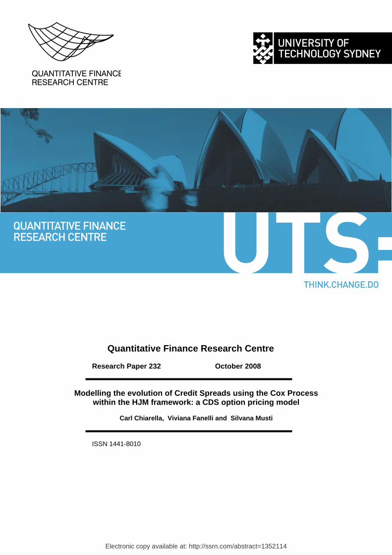
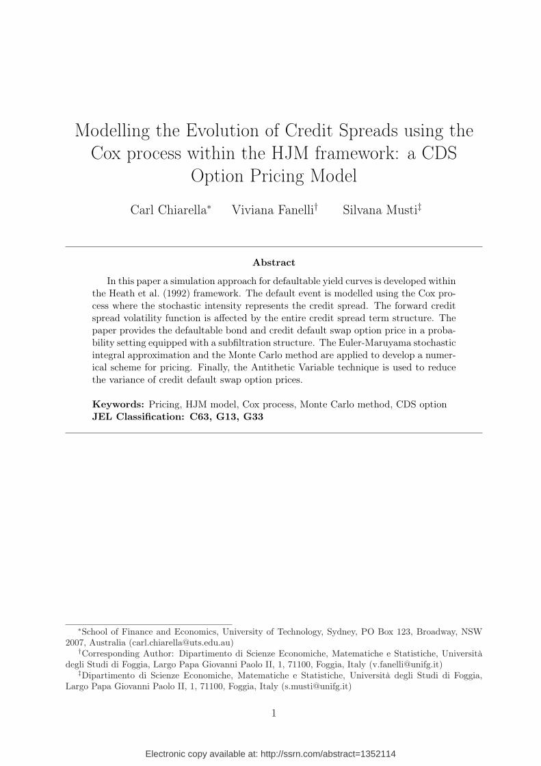
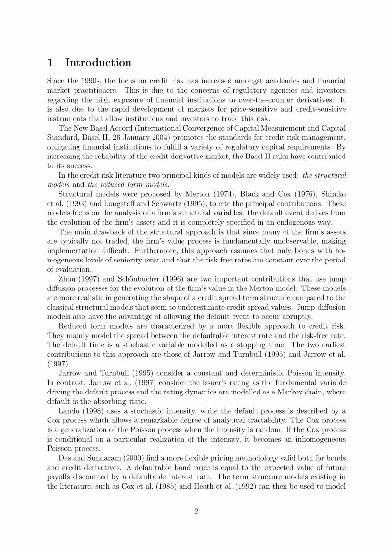
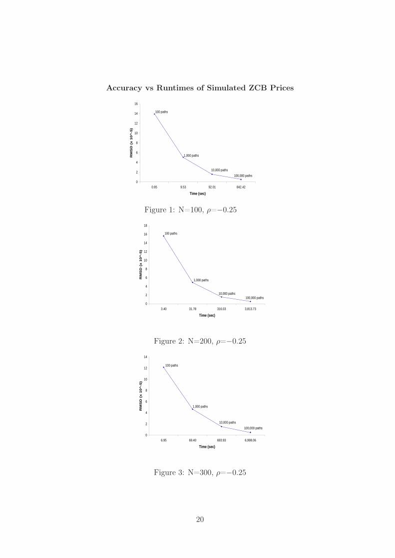
with Π = 100; 1, 000; 10, 000; 100, 000. In Table 7 we provide the RMSD values and the cor-responding runtimes for different N and Π in the case of positive and negative correlations.We find that increasing the number of paths, the pricing accuracy improves, confirmingthe previous considerations made about the results of the AV technique (Table 1). Clearly,both in the case of correlation coefficient equal to −0.25 and 0.25, the calculation is ob-tained faster when N = 100 than in the other cases. In particular, for each Π, the runtimetriples by increasing the discretisation from 100 to 200 and it doubles when N goes from200 to 300. In contrast, for a given Π, the accuracy basically remains unchanged whenN = 100, 200 and 300. For each N , by increasing the number of paths from 100 to 1,000the accuracy improves by one decimal place, while it remains basically unchanged movingfrom 1,000 to 10,000 paths. The best accuracy trade-off is obtained with 100,000 paths:for all discretisations the accuracy improves by two decimal places with respect to the oneobtained with Π = 100. This allows us to assert that the best efficiency trade-off of thenumerical scheme is obtained with N = 100, because runtimes are the lowest. With regardto the number of simulated paths, the choice will depend on the accuracy required. As wecan see from Table 7, the accuracy/runtimes results seem not to be influenced by the signof the correlation coefficient. For this reason we plot results only for ρ = −0.25 in Figures1-3. On the horizontal axis we measure the runtimes (seconds) on a logarithmic scale inorder to better highlight the computational time differences of the computed values. Onthe vertical axis the RMSDs are reported. The Figures are a more intuitive representationof the Table 7 data and they allow the reader to more readily appreciate the conclusionsdrawn above. It is evident that, for a given Π, as N increases, the runtime required toobtain a given accuracy increases. For example, a comparison of Figures 1 and 2 showsthat with 1,000 paths we can reach the accuracy of about 5 · 10−5 in 9.53 seconds if Nequals to 100, whereas we need 31.78 seconds if N equals to 200.

5 ConclusionsWe have developed an HJM model for the defaultable interest rate term structure whenthe forward rate volatility functions depend on time to maturity, on the instantaneous

15

defaultable spot rate and on the entire forward curve. The Cox process describes thedefault event and its intensity denotes the credit spread.

The described volatility functions are path dependent and therefore difficult to han-dle both analytically and numerically. Using a simple numerical scheme, based on theEuler-Maruyama discretisation for stochastic integrals, we develop a numerical approachto simulate the evolution of the entire defaultable curve over the time horizon in an efficientway. A more detailed discussion of the numerical scheme and further numerical results ofits implementation are provided by Fanelli (2007).

The expected bond value conditional on the realization of the Cox process intensity iscomputed by using an inhomogeneous Poisson process. In this way, the explicit reference tothe default event is eliminated and is defined as a function of the default process intensity.

We use the Monte Carlo method to calculate the defaultable bond price both in thecase of zero recovery rate and positive recovery rate. The numerical results indicate thenumerical scheme’s efficiency for evaluating corporate bonds and credit derivatives. Thedeveloped pricing numerical scheme also allows the evaluation of forward risky bond prices.Furthermore, we develop a numerical scheme for CDS and CDS option pricing. The An-tithetic Variable technique improves the accuracy of the simulated prices by reducing thestandard error.

The numerical analysis is completed with a study of the trade off between runtimesand accuracy, suggesting suitable combinations of number of paths/level of discretisation,in order to reach the accuracy required in the price evaluations. The analysis indicateshow the numerical scheme can be successfully utilized by credit risk practitioners in orderto price credit risk products with satisfactory levels of accuracy and reasonable runtimes.

As the number of credit derivatives grows continuously, new approaches for their eval-uation are required. Consequently, future research will need to develop new numericalschemes for the evaluations of other more exotic types of credit derivatives, such as basketproducts.

16

A Tables of Numerical Results

Table 1: I-Time zero ZCB Price

N = 100 ⇒ ExactPd(0, 1) = e−R 10 fd(0,s)ds ' 0.936794

ρ Paths Pd(0, 1) St. Err. PAV Td (0, 1) St. Err.AV T

-0.25 100 0.93672710 0.00089710 0.93704342 0.000136651,000 0.93580519 0.000329079 0.93680721 0.0000505910,000 0.93619924 0.00010088 0.93679236 0.00001571100,000 0.93637735 0.00003168 0.93678468 0.000004991,000,000 0.93634228 0.00001001 0.93679521 0.00000155

0.25 100 0.9367210 0.000897124 0.93703756 0.000136801,000 0.93579854 0.00032911 0.93680081 0.0000506510,000 0.93619275 0.00010089 0.93678590 0.00001572100,000 0.93637082 0.00003168 0.93677814 0.000005001,000,000 0.93633575 0.00001001 0.93678869 0.00000155

N = 200 ⇒ ExactPd(0, 1) = e−R 10 fd(0,s)ds ' 0.936850

ρ Paths Pd(0, 1) St. Err. PAV Td (0, 1) St.Err.AV T

-0.25 100 0.93616951 0.00096324 0.93698050 0.000155621,000 0.93655087 0.00031241 0.93692132 0.0000492110,000 0.93660845 0.00009928 0.93686060 0.00001541100,000 0.93668000 0.00003133 0.93684991 0.000004931,000,000 0.93663130 0.00000992 0.93685195 0.00000156

0.25 100 0.93616302 0.00096332 0.93697433 0.000155771,000 0.93654435 0.00031245 0.93691498 0.0000492610,000 0.93660200 0.00009929 0.93685412 0.00001543100,000 0.93667353 0.00003133 0.93684343 0.000004941,000,000 0.93662481 0.00000992 0.93684546 0.00000157

N = 300 ⇒ ExactPd(0, 1) = e−R 10 fd(0,s)ds ' 0.936869

ρ Paths Pd(0, 1) St. Err. PAV Td (0, 1) St.Err.AV T

-0.25 100 0.93695273 0.00084987 0.93726909 0.000114871,000 0.93704641 0.00030796 0.93691223 0.0000463210,000 0.93691862 0.00009831 0.93687990 0.00001531100,000 0.93678212 0.00003115 0.93687925 0.000004881,000,000 0.93672712 0.00000989 0.93687156 0.00000156

0.25 100 0.93694691 0.00084986 0.93726909 0.000114871,000 0.93704012 0.00030800 0.93691223 0.0000463210,000 0.93691207 0.00009832 0.93687990 0.00001531100,000 0.93677565 0.00003115 0.93687279 0.000004881,000,000 0.93672066 0.00000989 0.93686509 0.00000156

17

Table 2: Time zero ZCB Prices in the case of positive recovery rate (R)

R Exact Pd,R(0, 1) Paths Pd,R(0, 1) St. Err. PAV Td,R (0, 1) St. Err.AV T

0.27 0.93697471 100 0.93736910 0.00089803 0.93697471 0.000133941,000 0.93645934 0.00032909 0.93697471 0.0000496210,000 0.93685062 0.00010089 0.93697471 0.00001545

0.30 0.93699474 100 0.93738799 0.00089810 0.93722816 0.000133651,000 0.93647963 0.00032908 0.93700550 0.0000495310,000 0.93687058 0.00010088 0.93699106 0.00001542

0.36 0.93703481 100 0.93742577 0.00089824 0.93726511 0.000133091,000 0.93652021 0.00032906 0.93704516 0.0000493510,000 0.93691050 0.00010088 0.93703080 0.00001538

0.44 0.93708823 100 0.93747614 0.00089844 0.93728974 0.000132731,000 0.93657432 0.00032904 0.93709804 0.0000491410,000 0.93696373 0.00010087 0.93708378 0.00001532

Table 3: ZCB Futures Prices

ρ N Paths Pd(0, 2, 5) St.Err. PAV Td (0, 2, 5) St.Err.AV T

-0.25 500 100 0.77723533 0.00384184 0.77869190 0.001078191,000 0.77870174 0.00131634 0.77929703 0.0003961310,000 0.77930372 0.00041341 0.77931346 0.00010909

0.25 100 0.777138976 0.00383949 0.77859926 0.001077281,000 0.77859938 0.00131551 0.77919335 0.0003968410,000 0.77919522 0.00041326 0.77923799 0.00010945

ρ N Paths Pd(0, 5, 10) St.Err. Pd(0, 5, 10)AV T St.Err.AV T

-0.25 1,000 100 0.64604114 0.005267 0.64792752 0.003591921,000 0.65095188 0.00183757 n.a. n.a.

0.25 100 0.64589044 0.00525009 0.64774897 0.003604831,000 0.65072434 0.00183321 n.a. n.a.

n.a. = not available

Table 4: Time zero Credit Default Swaps on a risky zero coupond bond with R = 0.3 andmaturity of 3 years

Exact CDS=470.499 bpPaths CDS Rate St.Err. CDSAV T Rate St.ErrAV T

100 468.847 0.00073091 469.509 0.000268241,000 469.089 0.00027412 470.219 0.0001017210,000 469.498 0.00008365 n.a. n.a.

n.a. = not available

18

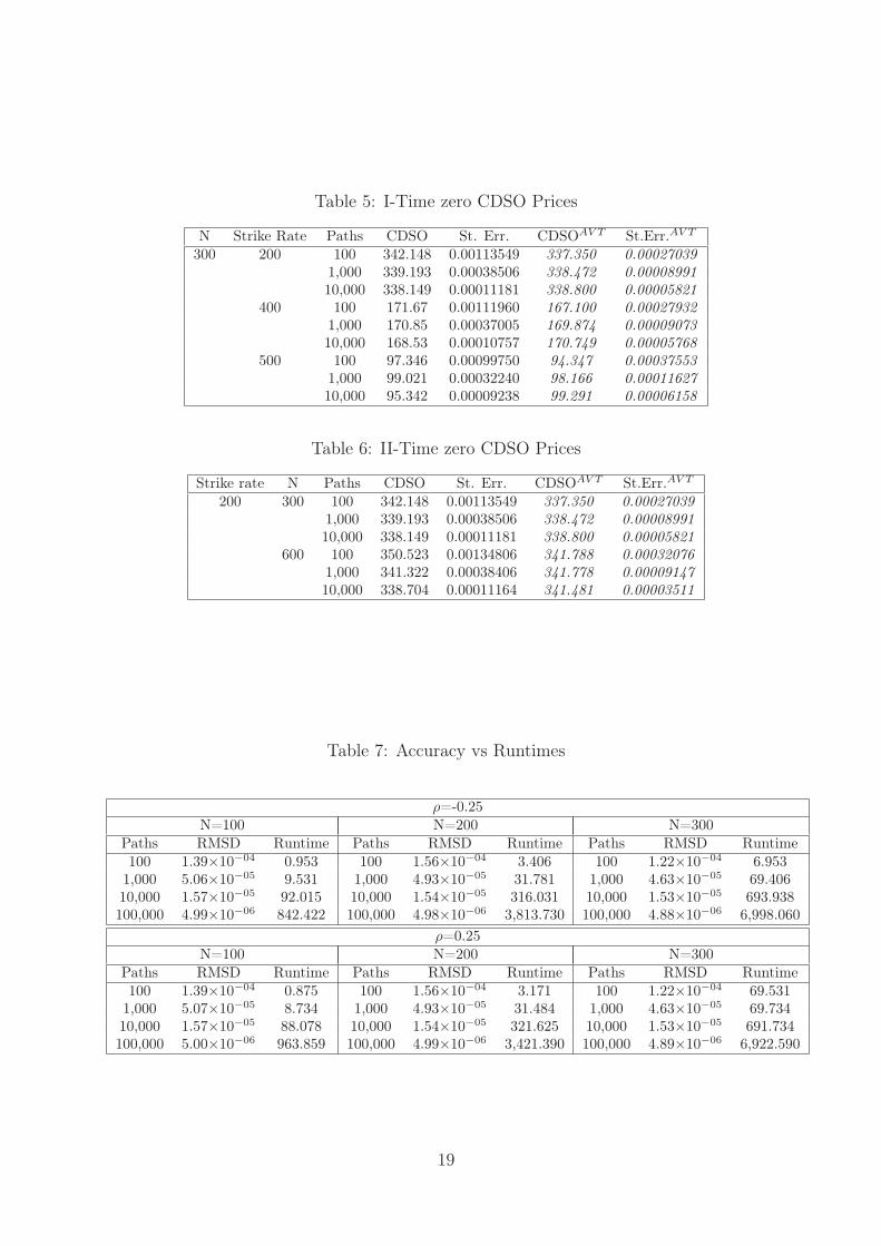
Table 5: I-Time zero CDSO Prices

N Strike Rate Paths CDSO St. Err. CDSOAV T St.Err.AV T

300 200 100 342.148 0.00113549 337.350 0.000270391,000 339.193 0.00038506 338.472 0.0000899110,000 338.149 0.00011181 338.800 0.00005821

400 100 171.67 0.00111960 167.100 0.000279321,000 170.85 0.00037005 169.874 0.0000907310,000 168.53 0.00010757 170.749 0.00005768

500 100 97.346 0.00099750 94.347 0.000375531,000 99.021 0.00032240 98.166 0.0001162710,000 95.342 0.00009238 99.291 0.00006158

Table 6: II-Time zero CDSO Prices

Strike rate N Paths CDSO St. Err. CDSOAV T St.Err.AV T

200 300 100 342.148 0.00113549 337.350 0.000270391,000 339.193 0.00038506 338.472 0.0000899110,000 338.149 0.00011181 338.800 0.00005821

600 100 350.523 0.00134806 341.788 0.000320761,000 341.322 0.00038406 341.778 0.0000914710,000 338.704 0.00011164 341.481 0.00003511

Table 7: Accuracy vs Runtimes

ρ=-0.25N=100 N=200 N=300

Paths RMSD Runtime Paths RMSD Runtime Paths RMSD Runtime100 1.39×10−04 0.953 100 1.56×10−04 3.406 100 1.22×10−04 6.9531,000 5.06×10−05 9.531 1,000 4.93×10−05 31.781 1,000 4.63×10−05 69.40610,000 1.57×10−05 92.015 10,000 1.54×10−05 316.031 10,000 1.53×10−05 693.938100,000 4.99×10−06 842.422 100,000 4.98×10−06 3,813.730 100,000 4.88×10−06 6,998.060

ρ=0.25N=100 N=200 N=300

Paths RMSD Runtime Paths RMSD Runtime Paths RMSD Runtime100 1.39×10−04 0.875 100 1.56×10−04 3.171 100 1.22×10−04 69.5311,000 5.07×10−05 8.734 1,000 4.93×10−05 31.484 1,000 4.63×10−05 69.73410,000 1.57×10−05 88.078 10,000 1.54×10−05 321.625 10,000 1.53×10−05 691.734100,000 5.00×10−06 963.859 100,000 4.99×10−06 3,421.390 100,000 4.89×10−06 6,922.590

19

Accuracy vs Runtimes of Simulated ZCB Prices

0

2

4

6

8

10

12

14

16

0.95 9.53 92.01 842.42

Time (sec)

RM

SD

(x 1

0^

-5)

100 paths

1,000 paths

100,000 paths

10,000 paths

Figure 1: N=100, ρ=−0.25

0

2

4

6

8

10

12

14

16

18

3.40 31.78 316.03 3,813.73

Time (sec)

RM

SD

(x 1

0^

-5)

1,000 paths

100 paths

10,000 paths100,000 paths

Figure 2: N=200, ρ=−0.25

0

2

4

6

8

10

12

14

6.95 69.40 693.93 6,998.06

Time (sec)

RM

SD

(x 1

0^

-5)

100 paths

1,000 paths

10,000 paths

100,000 paths

Figure 3: N=300, ρ=−0.25

20

B The HJM model for the defaultable term structureFrom equation (12) and the assumed dynamics of f(t, T ) and λs(t, T ), the HJM forwarddefaultable term structure dynamics may be expressed in the form

dfd(t, T ) = α(t, T, ·)dt + αλ(t, T, ·)dt + σ(t, T, ·)dW (t) + σλ(t, T, ·)dWλ(t). (44)

Integrating both sides, we obtain the instantaneous defaultable forward rate expressed inthe integral form

fd(t, T ) = f(0, T ) + λs(0, T ) +∫ t

0α(v, T, ·)dv +

∫ t

0αλ(v, T, ·)dv

+∫ t

0σ(v, T, ·)dW (v) +

∫ t

0σλ(v, T, ·)dWλ(v), (45)

where:

- f(0, T ) and λs(0, T ) are, respectively, the initial forward risk-free rate curve and theinitial forward spread curve, observable at time t = 0;

- α(t, T, ·) and αλ(t, T, ·) are the instantaneous drift functions of the risk-free forward rateand credit spread, where the third argument indicates the possible dependence onother path dependent variables, such as the spot rate, the forward rate itself or thecredit spread;

- σ(t, T, ·) and σλ(t, T, ·) are the instantaneous volatility functions of the risk-free forwardrate and credit spread, where, as above, the third argument indicates the aforemen-tioned possible dependence on other path dependent variables, such as the spot rate,the forward rate itself or the credit spread;

- W (t) and Wλ(t) are Wiener processes with respect to the objective probability measureP.

In the following, we denote the price of a defaultable ZCB with zero recovery rate asPd(t, T ). Therefore, in the case of no default, we have:

Pd(t, T ) = e−R T

t fd(t,s)ds = e−R T

t (f(t,s)+λs(t,s))ds. (46)

By the use of Fubini’s Theorem for the stochastic integral and application of Ito’s lemma,the defaultable bond price is found to satisfy the stochastic differential equation

dPd(t, T ) = [r(t) + λ(t) + b(t, T ) + bλ(t) + ρa(t, T )aλ(t, T )]Pd(t, T )dt

+a(t, T )Pd(t, T )dW (t) + aλ(t, T )Pd(t, T )dWλ(t), (47)

where

a(v, t) = − ∫ t

vσ(v, s)ds,

aλ(v, t) = − ∫ t

vσλ(v, s)ds,

(48)

21

and

b(v, t) = − ∫ t

vα(v, s)ds + 1

2a(v, t)2,

bλ(v, t) = − ∫ t

vαλ(v, s)ds + 1

2aλ(v, t)2.

(49)

Equation (47) can be also written in return form as

dPd(t, T )

Pd(t, T )= [r(t) + λ(t) + b(t, T ) + bλ(t) + ρa(t, T )aλ(t, T )]dt

+a(t, T )dW (t) + aλ(t, T )dWλ(t). (50)

In order to obtain the no arbitrage condition, we start from (50) and apply the Schön-bucher (1998) approach and the Björk (2004) methodology. That is we apply the economicprinciple that the expected excess return on the defaultable bond is equal to the risk pre-mium. Thus keeping in mind that a(t, T ) and aλ(t, T ) are respectively “the amounts ofrisk” associated with the Wiener increments dW (t) and dWλ(t) we write

[r(t) + b(t, T ) + bλ(t, T ) + ρa(t, T )aλ(t, T )]− r(t) =

φ(t)a(t, T ) + φλ(t)aλ(t, T ), (51)

where φ is the market price of interest rate (W (t)) risk and φλ is the price of spread (Wλ(t))risk. Equation (51) is the “martingale measure equation”. It allows the transition fromthe actual risky world under the objective P measure to the risk neutral world under themeasure P. On the left-hand side we have the excess rate of return for the defaultablebond over the risk-free rate, and on the right-hand side we have the linear combinationof the volatilities and market prices of risk that combine to yield the instantaneous riskpremium. Some simple rearrangements express (51) in the more convenient form

b(t, T )− φ(t)a(t, T ) + bλ(t, T )− φλ(t)aλ(t, T ) + ρa(t, T )aλ(t, T ) = 0. (52)

By substituting (48) and (49) into (52) we obtain

−∫ T

t

α(t, s)ds +1

2

(∫ T

t

σ(t, s)ds

)2

−∫ T

t

αλ(t, s)ds

+1

2

(∫ T

t

σλ(t, s)ds

)2

+ ρ

∫ T

t

σ(t, s)ds

∫ T

t

σλ(t, s)ds

+φ(t)

∫ T

t

σ(t, s)ds + φλ(t)

∫ T

t

σλ(t, s)ds = 0. (53)

By differentiating with respect to T, the above expression can be rewritten in the form

−α(t, T ) + σ(t, T )

∫ T

t

σ(t, s)ds− αλ(t, T )

+σλ(t, T )

∫ T

t

σλ(t, s)ds + ρσ(t, T )

∫ T

t

σλ(t, s)ds

+ρσλ(t, T )

∫ T

t

σ(t, s)ds− φ(t)σ(t, T )− φλ(t)σλ(t, T ) = 0. (54)

22

From (54) we can obtain the HJM forward rate drift restriction for defaultable processes,namely

αd(t, T ) = α(t, T ) + αλ(t, T )

= σ(t, T )

∫ T

t

σ(t, s)ds + σλ(t, T )

∫ T

t

σλ(t, s)ds

+ρ

[σ(t, T )

∫ T

t

σλ(t, s)ds + σλ(t, T )

∫ T

t

σ(t, s)ds

]

−φ(t)σ(t, T )− φλ(t)σλ(t, T ). (55)

We define two new processes

W (t) = W (t) +

∫ t

0

(−φ(s))ds, (56)

and

Wλ(t) = Wλ(t) +

∫ t

0

(−φλ(s))ds, (57)

so that

dW (t) = dW (t)− φ(t)dt, (58)

and

dWλ(t) = dWλ(t)− φλ(t)dt. (59)

For later calculations we note that the last two equations imply that

dW (t) = dW (t) + φ(t)dt, (60)

anddWλ(t) = dWλ(t) + φλ(t)dt. (61)

By an application of Girsanov’s Theorem W (t) and Wλ(t) will be Wiener processes underP. By substituting (55), (60) and (61) into (44) we obtain

dfd(t, T ) =

[σ(t, T )

∫ T

t

σ(t, s)ds + σλ(t, T )

∫ T

t

σλ(t, s)ds

+ρσ(t, T )

∫ T

t

σλ(t, s)ds + ρσλ(t, T )

∫ T

t

σ(t, s)ds

]dt

+σ(t, T )dW (t) + σλ(t, T )dWλ(t). (62)

By integrating, we obtain the instantaneous defaultable forward rate dynamics in stochasticintegral equation form, namely

fd(t, T ) = f(0, T ) + λs(0, T )

+

∫ t

0

[σ(v, T )

∫ T

v

σ(v, s)ds + σλ(v, T )

∫ T

v

σλ(v, s)ds

]dv

+

∫ t

0

ρ

[σ(v, T )

∫ T

v

σλ(v, s)ds + σλ(v, T )

∫ T

v

σ(v, s)ds

]dv

+

∫ t

0

[σ(v, T )dW (v) + σλ(v, T )dWλ(v)

]. (63)

23

From (63) we derive the defaultable spot rate process rd(t) = fd(t, t), so that

rd(t) = f(0, t) + λs(0, t)

+

∫ t

0

[σ(v, t)

∫ t

v

σ(v, s)ds + σλ(v, t)

∫ t

v

σλ(v, s)ds

]dv

+

∫ t

0

ρ

[σ(v, t)

∫ t

v

σλ(v, s)ds + σλ(v, t)

∫ t

v

σ(v, s)ds

]dv

+

∫ t

0

[σ(v, t)dW (v) + σλ(v, t)dWλ(v)

]. (64)

From (55) and (5) we deduce the HJM credit spread drift condition, which can be written

αλ(t, T ) = ρ

[σ(t, T )

∫ T

t

σλ(t, s)ds + σλ(t, T )

∫ T

t

σ(t, s)ds

]

+σλ(t, T )

∫ T

t

σλ(t, s)ds− φλ(t)σλ(t, T ) . (65)

As in the default free HJM model, the derivative security price is evaluated independentlyof the market prices of risk, because they get absorbed in the change of measure to P,under which the spot rate and bond price processes are expressed in the arbitrage freedynamics. Finally we derive the bond pricing formula under P.

We start by choosing the numeraire

Bd(t) = eR t0 rd(s)ds,

so that relative bond price is given by

Z(t, T ) =Pd(t, T )

Bd(t)= Pd(t, T )e−

R t0 rd(t)ds. (66)

By applying Ito’s Lemma to (66) and recalling the definitions (48) and (49), we obtain

dZ(t, T ) = [b(t, T )Z(t, T ) + bλ(t, T )Z(t, T )] dt

+a(t, T )Z(t, T )dW + aλ(t, T )Z(t, T )dWλ. (67)

By Girsanov’s Theorem and using relation (52), the process (67) can be written in termsof the Brownian motions (58) and (59) generated by the equivalent martingale probabilitymeasure P, thus we write

dZ(t, T ) = a(t, T )Z(t, T )dW (t) + aλ(t, T )Z(t, T )dWλ(t). (68)

Since the stochastic differential equation is driftless, Z(t, T ) is a martingale under theprobability measure P and the bond value is calculated as the expected value with respectto the probability measure P with expected future payoffs discounted using the defaultablerate rd(t), that is

Pd(t, T ) = EeP[e−

R tt rd(s)ds

]. (69)

The above evaluation rule may be applied to price any derivative security within the HJMframework. An exhaustive mathematical explanation of the risk neutral valuation principleis given in Bielecki and Rutkowski (2001).

24

ReferencesBielecki, T. & Rutkowski, M. (2001). Credit risk: Modeling, Valuation and Hedging.

Springer Verlag.

Björk, T. (2004). Arbitrage Theory in Continuous Time, (second ed.). OXFORD Finance.

Black, F. & Cox, J. (1976). Valuing Corporate Securities: Some Effects of Bond IndentureProvisions. Journal of Finance, 31(2):351–367.

Brigo, D. & Morini, M. (2005). CDS Market Formulas and Models. In: Proceedings of the18th Annual Warwick Options Conference, September 30, 2005, Warwick, UK.

Chen, R., Cheng, X., Fabozzi, F. J., & Liu, B. (2008). An explicit, multi-factor credit de-fault swap pricing model with correlated factors. Journal of Financial and QuantitativeAnalysis, 43(1):123–160.

Chiarella, C., Clewlow, L., & Musti, S. (2005). A volatility decomposition control vari-ate technique for Monte Carlo simulations of Heath Jarrow Morton models. EuropeanJournal of Operational Research, 161(2):325–336.

Cox, J., Ingersoll, J., & Ross, S. (1985). A theory of the term structure of interest rates.Econometrica, 53:385–407.

Das, S. & Sundaram, R. (2000). A Discrete-Time Approach to Arbitrage-Free Pricing ofCredit Derivatives. Management Science, 46(1):46–62.

Duffie, D. & Lando, D. (2001). Term structures of credit spreads with incomplete account-ing information. Econometrica, 69:633–664.

Duffie, D. & Singleton, K. (1999). Modelling Term Structures of Defaultable Bonds. Reviewof Financial Studies, 12:687–720.

Fanelli, V. (2007). Numerical implementation of a credit risk model in the HJM framework.PhD thesis, Dipartimento di Scienze Economiche, Matematiche e Statistiche, Universitàdi Foggia.

Heath, D., Jarrow, R., & Morton, A. (1992). Bond Pricing and the Term Structure ofInterest Rates: A New Methodology for contingent claims valuation. Econometrica,60(1):77–105.

Hull, J. & White, A. (2000). Valuing credit default swaps I: No counterparty default risk.Journal of Derivatives, 8(1):29–40.

Hull, J. & White, A. (2001). Valuing credit default swaps II: Modeling default correlations.Journal of Derivatives, 8(3):12–22.

Jamshidian, F. (2004). Valuation of credit default swaps and swaptions. Finance andStochastics, 8(3):343–371.

Jarrow, R., Lando, D., & Turnbull, S. (1997). A Markov Model for the Term Structure ofCredit Spreads. Review of Financial Studies, 10:481–523.

25

Jarrow, R. A. & Turnbull, S. M. (1995). Pricing Derivatives on Financial Securities Subjectto Credit Risk. Journal of Finance, 50(1):53–85.

Jeanblanc, M. & Rutkowski, M. (2002). Default risk and hazard process, pages 281–312.In Mathematical Finance - Bachelier Congress 2000. H. Geman, D. Madan, S.R. Pliskaand T. Vorst, eds., Springer-Verlag, Berlin, 2002.

Kloeden, P. & Platen, E. (1999). Numerical Solution of Stochastic Differential Equations.Springer-Verlag.

Lando, D. (1998). On Cox Processes and Credit Risky Securities. Review of DerivativesResearch, 2(2/3):99–120.

Longstaff, F. & Schwartz, E. (1995). The pricing of credit risk derivatives. Journal ofFixed Income, 5(1):6–14.

Maksyumiuk, R. & Gatarek, D. (1999). Applying HJM to credit risk. Risk, 12(5):67–68.

Merton, R. (1974). On the pricing of corporate debt: The Risk Structure of Interest Rates.The Journal of Finance, 29:449–470.

Moody’s Investors Service (2007). EUROPEAN CORPORATE DEFAULT AND RECOV-ERY RATES, 1982-2006.

Pugachevsky, D. (1999). Generalizing with HJM. Risk, 12:103–105.

Schönbucher, P. (1996). Valuation of securities subject to credit risk, University of Bonn,Department of Statistics, retrieved May 10, 2006, from http://www.schonbucher.de.

Schönbucher, P. (1998). Term structure modelling of defaultable bonds. Review of Deriva-tives Research, 2:123–134.

Shimko, D., Tejima, N., & Deventer, D. (1993). The Pricing of Risky Debt when InterestRates are Stochastic. Journal of Fixed Income, pages 58–66.

Zhou, C. (1997). Jump-diffusion approach to modeling credit risk and valuing defaultablesecurities, Finance and Economics Discussion Paper Series 1997/15, Board of Governorsof the Federal Reserve System.

26