MODELLING OF MULTIPLE DELAMINATIONS IN SHELLS USING XFEMconfsys.encs.concordia.ca/ICCM19/AllPapers/FinalVersion/BRO81242.pdf · THE 19TH INTERNATIONAL CONFERENCE ON COMPOSITE MATERIALS

THE 19TH INTERNATIONAL CONFERENCE ON COMPOSITE MATERIALS

MODELLING OF MULTIPLE DELAMINATIONS IN SHELLS USING XFEM

J. Brouzoulis1∗, M. Fagerstrom1

Department of Applied Mechanics, Chalmers University of Technology, Goteborg, Sweden∗Corresponding author ([email protected])

Keywords: multiple delaminations, XFEM, shell theory

1 Introduction

There is an ever increasing interest in utilising FiberReinforced Polymers (FRP) in the automotive indus-try, especially for structural components. This callsfor computational tools which can be used for theevaluation of crashworthiness. One key point is theneed for computational efficiency as the models aregenerally very complex. Furthermore, there is amultitude of failure mechanisms which may be trig-gered in a layered composite, during impact or crash,with multiple delaminations being one of the primarymechanisms.

It is therefore of high importance to be able to modeldelaminations in a computationally efficient manner,especially for a large number of laminae. In fact, to beable to simulate the progressive failure of FRP com-ponents is a necessity for such components to be com-petitive within the automotive industry, as e.g. statedin the ERTRAC Research and Innovation Roadmapfor Safe Road Transport [1].

In view of this, this work is a first step towards devel-oping a computationally efficient shell element whichcan account for multiple (interlaminar) delaminations.One commonly adopted approach is to model each in-dividual ply (or a set of plies) using several stackedshell or solid elements. However, this will lead to alarge amount of degrees of freedom, especially whenthe number of plies increases. Another, more econom-ical, approach is to use a single shell element whichcan account (internally) for the discontinuities that de-velop during delamination. Such an element may beconstructed by enriching a suitable shell element withdiscontinuous shape functions in accordance with theeXtended Finite Element Method (XFEM), cf. [2] for

a similar approach. Note that the present approachis similar to a layerwise model where displacementsjumps are hierarchically added to the displacementsfield, cf. e.g. [3].

2 Continuous shell kinematics

To set the stage, we first briefly describe the under-lying shell kinematics for a non-delaminated shell,which in the subsequent section then will be extendedto allow for arbitrarily many delaminations.

2.1 Initial shell geometry and convected coordi-nates

As a staring point, the initial configuration B0 of theshell is considered parameterised in terms of con-vected (covariant) coordinates (ξ1, ξ2, ξ) as

B0 =X := Φ(ξ) = Φ(ξ) + ξM(ξ)

with ξ ∈ A and ξ ∈ h02 [−1, 1]

(1)

where we introduced the contracted notation ξ =(ξ1, ξ2, ξ) and ξ = (ξ1, ξ2) and where the mappingΦ(ξ) maps the inertial Cartesian frame into the un-deformed configuration, cf. Figure 1. Furthermore,A is the midsurface of the inertial configuration. InEq. (1), the mapping Φ is defined by the midsurfaceplacement Φ and the outward unit normal vector fieldM (with |M | = 1). The coordinate ξ is associatedwith this direction and h0 is the initial thickness of theshell.

Furthermore, it should be noted that

dX = (Gα ⊗Gα) · dX +M ⊗M · dX =

= Gα(ξ)dξα +M(ξ)dξ (2)

whereby the covariant basis vectors are defined by

Gα = Φ,α + ξM ,α α = 1, 2 (3)

G3 = G3 = M (4)

where •,α denotes the derivative with respect to ξα. Inaddition, in Eq. (2) it was used that the contravariantbasis vectorsGi are associated with the covariant vec-tors Gi in the normal way, i.e. Gi ⊗Gi = I, leadingto

Gj = GijGi, Gj = GijGi (5)

with

Gij = Gi ·Gj and Gij = (Gij)−1 (6)

Finally, the infinitesimal volume element dB0 of thereference configuration is formulated in the convectedcoordinates as

dB0 = b0dξ1dξ2dξ with b0 = (G1 ×G2) ·G3 (7)

2.2 Current shell geometry

The current (deformed) geometry is in the present for-mulation described by the time dependent deforma-tion map ϕ(ξ, t) ∈ B of the inertial Cartesian frameas

x(ξ, t) = ϕ(ξ, t) + ξm(ξ, t) +1

2ξ2γ(ξ, t)m(ξ, t)

(8)where the mapping is defined by the midsurface place-ment ϕ, the spatial director field m and an additionalscalar thickness inhomogeneity strain γ, cf. Figure 1.As can be seen, the specification of the current config-uration corresponds to a second order Taylor expan-sion along the director field, involving the inhomo-geneity strain γ, thereby describing inhomogeneousthickness deformation effects of the shell. In particu-lar, the pathological Poisson locking effect is avoidedin this fashion.

To identify the corresponding deformation gradient,a relative motion dx of the placement map ϕ withrespect to the reference placement Φ is considered as

dx = F · dX with F =∂ x

∂ ξ

∂ ξ

∂X= gi ⊗Gi (9)

where the spatial covariant basis vectors gi = ∂x/∂ξiare identified as

gα = ϕ,α +

(ξ +

1

2γξ2

)m,α +

1

2γ,αξ

2m (10)

g3 = (1 + γξ)m (11)

3 XFEM extension for multiple delaminations

As stated above, the primary focus of the current workis to develop a shell element formulation able to rep-resent arbitrarily many delaminations within one ele-ment. Consequently, the above basic shell kinematicsneed to be extended to allow for displacement and di-rector discontinuities across each delamination inter-face. For this purpose, we propose herein a kinemat-ical extension in line with the XFEM (or partition ofunity concept) such that the deformation map into thespatial deformed configuration is subdivided into onecontinuous and one discontinuous part as

x(ξ, t) = ϕc(ξ, t) +ϕd(ξ, t) (12)

where the continuous part takes on the same form asthe underlying non-delaminated shell element

ϕc(ξ, t) = ϕc(ξ, t)+ξmc(ξ, t)+1

2ξ2γ(ξ, t)mc(ξ, t)

(13)As for the discontinuous part, it is considered as a sumof enrichments – one for each delamination – accord-ing to the XFEM, however restricted only to discon-tinuous enrichment of the midsurface placement andthe director field. Hence, in the case of Ndel delami-nations through the thickness, the discontinuous parttakes on the following form

ϕd(ξ) =

Ndel∑

k=1

HS (Sk(X, t))(ϕdk(ξ, t) + ξmd

k(ξ, t))

= HSk

(ϕdk + ξmd

k

)(sum over k)

(14)

In Eq. (14), HS(Sk(X)) = HSkis introduced as the

standard Heaviside function pertaining to the particu-lar delamination surface ΓSk

. Furthermore, Sk is anassociated level set function defining the position ξk(in thickness direction) of this surface. In particular,

M

G1

G2

A, V

Ω0, B0

Ω, B

mg2

g1

E1

E2

E3

Inertial configuration

F

Φ

Reference configuration

ϕ

Current configuration

Figure 1: Mappings of shell model defining undeformed and deformed shell configurations relative to inertialCartesian frame.

Sk is the signed distance function to the delaminationinterface k such that, for the current approach wherewe restrict the initial director field to coincide with theoutward normal vector, it can be defined simply as

Sk = ξ − ξk whereby∂ Sk∂X

= M (15)

where M is the normal to each delamination sur-face in the reference configuration. To obtain the cor-responding deformation gradient, we first emphasisethat

∂ HSk

∂X=∂ HSk

∂ Sk

∂ Sk∂X

= δSkM (16)

where δSk is the Dirac-delta function defined as∫

B0δSk • dB0 =

∫

ΓSk

• dΓSk (17)

for any quantity •.

Consequently, in analogy with Eq. (9)-(11), the defor-mation gradient pertaining to the extended kinematicsis obtained in the form

F =(ϕc +ϕd

)⊗∇X = F b + δSkF

dk (18)

whereF b = gb

j ⊗Gj , j = 1, 2, 3 (19)

andF dk =

(ϕdk + ξmd

k

)⊗M (20)

layer

delamination

discontinuity jumppointwise map

ξ

−h0

2

h0

2

ξ1

ξ2

ξNdel

ϕc

ϕc + ϕd1

ϕc + ϕd1 + ϕd

2

ϕc +∑Ndel

k=1 ϕdk

Figure 2: Illustration of a laminate subject to multipledelaminations.

The corresponding spatial covariant basis vectors areobtained as

gbα = ϕc

,α +

(ξ + γ

1

2ξ2

)mc

,α + γ,α1

2ξ2mc

+

Ndel∑

k=1

HSk

(ϕdk,α + ξmd

k,α

) (21)

gb3 = (1 + γξ)mc +

Ndel∑

k=1

HSkmd

k (22)

4 Weak form of momentum balance

In this section, we establish the momentum balanceof the shell considering the weak continuum repre-sentation of the shell applied to the shell kinematicsintroduced above. To arrive at the current stress resul-tant formulation, we start from the basic weak form ofthe momentum balance in terms of contributions frominertia W ine, internal work W int and external workWext as

Find: n such that:

W ine(

¨n; δn)

+W int (n; δn) (23)

+Wext (n; δn) = 0 ∀δn

where we introduced the array of solution fields

nT =(ϕc,mc, γ, ϕd

k,mdk

)(24)

where, for example, ϕdk refers to the array

(ϕd1 , ϕ

d2 , . . . , ϕ

dNdel

) and represents the additional dis-continuity fields associated with the existing delami-nations. Furthermore, the inertia and the internal andexternal virtual work contributions are given as

W ine =

∫

B0ρ0

(δϕc + δϕd

)·(ϕc + ϕd

)dB0,

(25)

W int =

∫

B0

(δFT · F

): SdB0 (26)

and

Wext =

∫

B0ρ0

(δϕc + δϕd

)· b dB0

+

∫

∂B0

(δϕc + δϕd

)· t1dΩ0

(27)

where b is the body force per unit volume, t1 =P ·N∂B0 is the nominal traction vector on the outerboundary ∂B0 and P = F ·S is the first Piola Kirch-hoff stress tensor.

To obtain the explicit form of each individual term inEqs. (25)-(27), we start by concluding that the inertiapart is given by

W ine =

∫

B0ρ0

(δϕc +HSk

δϕdk

)·(ϕc +HSlϕ

dl

)dB0

=

∫

Ω0

ρ0δnT(M ¨n+ M con) dΩ0

(28)

where the consistent mass matrix M and the convec-tive mass force M

conper unit area are obtained us-

ing a similar strategy as in Reference [4], although ac-counting for the alternative discontinuity enrichment.Note that, M con involves contributions from the firstorder time derivatives of the displacement field in theinertia term of the virtual work as described in Refer-ence [5]. Furthermore, in order to arrive at Eq. (28), achange of the integration domain from B0 (3D) to Ω0

(2D) was made via the ratio j0(ξ) = b0/ω0 definingthe relation between area and volumetric measures ofthe shell defined as

dB0 = j0dξdΩ0 with

dΩ0 = ω0dξ1dξ2 and ω0 = |Φ,1 ×Φ,2|(29)

Furthermore, when limiting the perpendicular forcesto external pressure – approximated in view of theCauchy traction t = −pn on the deformed midsur-face Ω – the external workWext can be written as

Wext =

∮

∂Ω0

(δϕc · N c

+ δmc · M c+ δγMs

c)

ds

+

∮

∂Ω0

(δϕd

k · Ndk + δmd

k · Mdk

)ds

−∫

Ωp(δϕc + δϕd

)· n dΩ

(30)

where p = p (t, ξ1, ξ2) is the external pressure, n isthe spatial normal of the deformed midsurface Ω andwhere N

c, M

c, Ms

c, N

dk and M

dk are stress resul-

tants with respect to the prescribed in-plane traction

acting on the outer boundary (perpendicular to themidsurface), defined as

Nc

=

∫ h0/2

−h0/2t1dξ (31)

Mc

=

∫ h0/2

−h0/2ξ

(1 +

1

2ξγ

)t1dξ (32)

Msc

=

∫ h0/2

−h0/2

1

2ξ2mc · t1dξ (33)

Ndk =

∫ h0/2

−h0/2HSk

t1dξ =

∫ h0/2

ξk

t1dξ (34)

Mdk =

∫ h0/2

−h0/2HSk

ξt1dξ =

∫ h0/2

ξk

ξt1dξ (35)

To obtain the explicit form of the internal virtual workcontribution we first note that this contribution can bereformulated, given the present kinematical represen-tation, as

W int =

∫

B0

(δF bT · F b

): S dB0

+

Ndel∑

k=1

∫

ΓSk

(δϕd

k + ξδmdk

)· tcoh(Jϕd

kK)dΩ0

(36)

where tcoh is the (continuous) degrading normal trac-tion on the delamination surface (with respect to theoutward pointing normal M ), which in the presentapproach will be represented by a cohesive zone lawas a function of the delamination discontinuity

JϕdkK =

(ϕdk + ξkm

dk

), (37)

cf. Section 5 below. Based on this, we note that the’internal work’ can be written as

W int =

∫

Ω0

δnTc N cdΩ0 +

∫

Ω0

δnTd NddΩ0

+

Ndel∑

k=1

∫

ΓSk

(δϕd

k + ξδmdk

)· tcoh(Jϕd

kK)dΩ0

(38)

where the shell deformation and stress resultant vec-

tors have been introduced as

δnTc =

[δϕc

,α,mc,α, δm

c, δγ,α, δγ]

δnTd =

[δϕd

k,α, δmdk,α, δm

dk

]

NTc = [N cα,M cα,T c,M cα

s , T cs ]

NTd =

[Ndα

k ,Mdαk ,T d

k

]

(α = 1, 2) involving the membrane, bend-ing, shear/thickness stretch stress resultantsNα,Mα,T ,Ndα

k ,Mdαk ,T d

k (the three latter beingconjugated with the discontinuous displacementvariables) and the higher order stress resultants Mα

s

and Ts. By introducing the abbreviation Sαigi = sαgthe explicit expressions for the stress resultants canbe written

Nα =

∫ h0/2

−h0/2sαg j0dξ (39)

Mα =

∫ h0/2

−h0/2

(1 +

1

2γξ

)ξsαg j0dξ (40)

T =

∫ h0/2

−h0/2

((1 + γξ) s3

g +1

2ξ2sαg γ,α

)j0dξ

(41)

Mαs =

∫ h0/2

−h0/2

1

2ξ2sαg ·mcj0dξ (42)

Ts =

∫ h0/2

−h0/2(1

2ξ2sαg ·mc

,α + ξs3g ·mc)j0dξ

(43)

Ndαk =

∫ h0/2

ξk

sαg j0dξ (44)

Mdαk =

∫ h0/2

ξk

ξsαg j0dξ (45)

T dk =

∫ h0/2

ξk

s3gj0dξ (46)

Finally, by substituting the displacement field into theweak form we are given the equation of motion as

Ma = f ext −M con − bint − bcoh (47)

where bint, bcoh, and f ext, denote internal, cohesiveand external forces respectively.

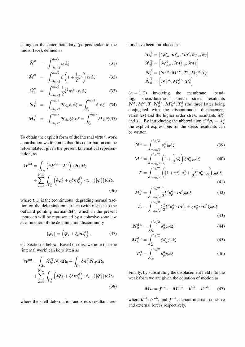
σn

σfn

g0g = Jϕd

kKgmax

Figure 3: Bilinear cohesive zone law adopted in thecurrent paper.

5 Modelling of progressive delamination

As indicated in Section 4, the progressive inter–laminar fracture process (delamination) is modelledusing a cohesive zone approach. Furthermore, by in-troducing a cohesive zone model, interpenetration ofthe layers is avoided allowing for a realistic represen-tation of the (interlaminar) kinematics.

5.1 Cohesive zone model

In this paper, a bilinear cohesive zone model, cf. Fig-ure 3, is adopted instead of a more refined model sincethe focus of this study is on the (extended) kinemat-ics. Furthermore, it keeps the modelling complexityto a minimum. Also note that the chosen cohesive lawis purely elastic such that any unloading would followthe loading path in reverse; however, only exampleswith monotonic loading is studied in the present pa-per such that this non-physical unloading behaviour isavoided.

6 Numerical examples

To illustrate the proposed kinematics, three numericalexamples are presented. The first example concernssimulation of the common double cantilever beam(DCB) test with the purpose of validating the kine-matics of the element under progressive delamination.The second example illustrates the capability of the el-ement formulation to kinematically represent two de-laminations within a single element. The final exam-

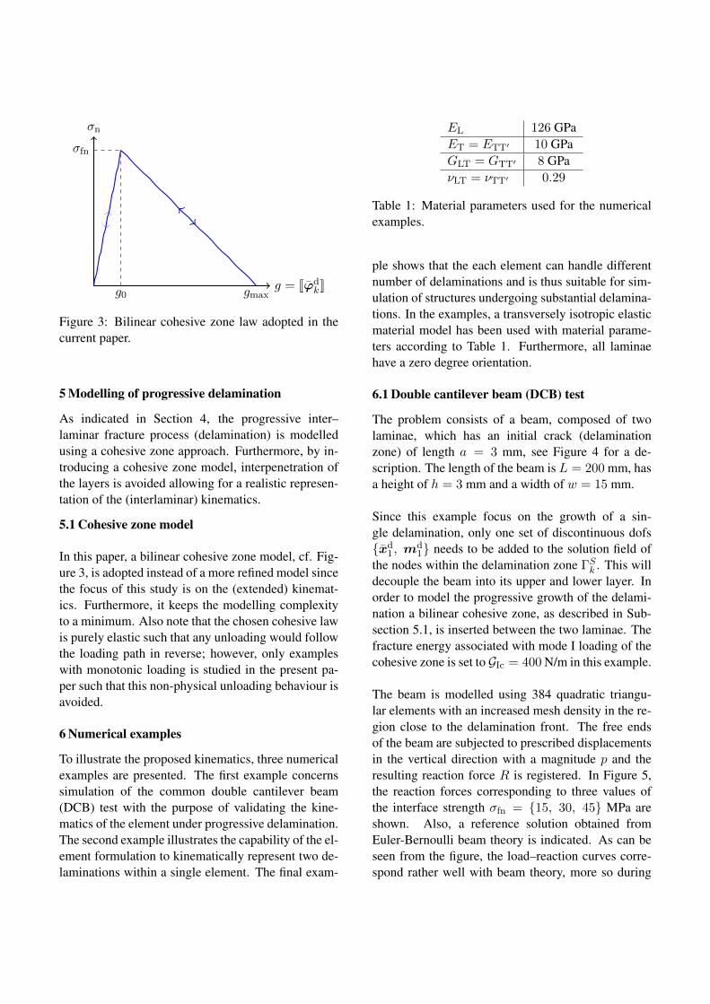
EL 126 GPaET = ETT′ 10 GPaGLT = GTT′ 8 GPaνLT = νTT′ 0.29

Table 1: Material parameters used for the numericalexamples.

ple shows that the each element can handle differentnumber of delaminations and is thus suitable for sim-ulation of structures undergoing substantial delamina-tions. In the examples, a transversely isotropic elasticmaterial model has been used with material parame-ters according to Table 1. Furthermore, all laminaehave a zero degree orientation.

6.1 Double cantilever beam (DCB) test

The problem consists of a beam, composed of twolaminae, which has an initial crack (delaminationzone) of length a = 3 mm, see Figure 4 for a de-scription. The length of the beam is L = 200 mm, hasa height of h = 3 mm and a width of w = 15 mm.

Since this example focus on the growth of a sin-gle delamination, only one set of discontinuous dofsxd

1 , md1 needs to be added to the solution field of

the nodes within the delamination zone ΓSk . This willdecouple the beam into its upper and lower layer. Inorder to model the progressive growth of the delami-nation a bilinear cohesive zone, as described in Sub-section 5.1, is inserted between the two laminae. Thefracture energy associated with mode I loading of thecohesive zone is set to GIc = 400 N/m in this example.

The beam is modelled using 384 quadratic triangu-lar elements with an increased mesh density in the re-gion close to the delamination front. The free endsof the beam are subjected to prescribed displacementsin the vertical direction with a magnitude p and theresulting reaction force R is registered. In Figure 5,the reaction forces corresponding to three values ofthe interface strength σfn = 15, 30, 45 MPa areshown. Also, a reference solution obtained fromEuler-Bernoulli beam theory is indicated. As can beseen from the figure, the load–reaction curves corre-spond rather well with beam theory, more so during

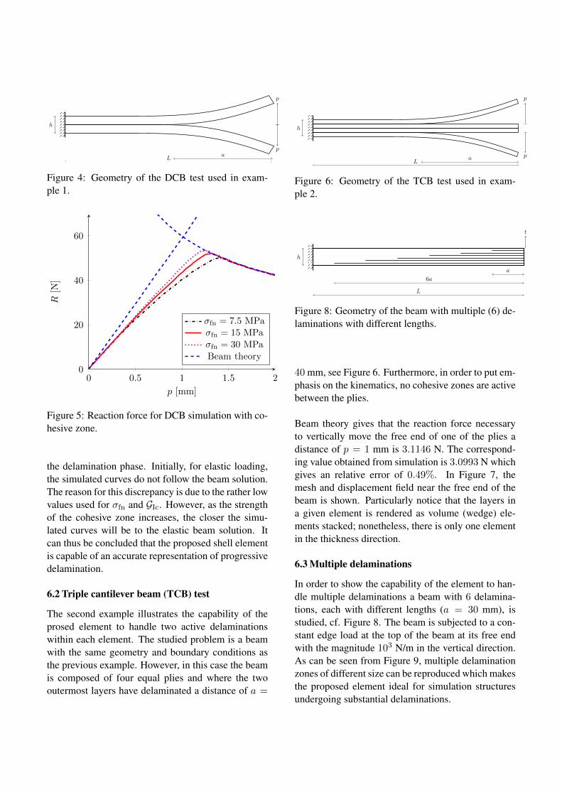
p

pa

L

h

Figure 4: Geometry of the DCB test used in exam-ple 1.

0 0.5 1 1.5 20

20

40

60

p [mm]

R[N

]

σfn = 7.5 MPaσfn = 15 MPaσfn = 30 MPaBeam theory

Figure 5: Reaction force for DCB simulation with co-hesive zone.

the delamination phase. Initially, for elastic loading,the simulated curves do not follow the beam solution.The reason for this discrepancy is due to the rather lowvalues used for σfn and GIc. However, as the strengthof the cohesive zone increases, the closer the simu-lated curves will be to the elastic beam solution. Itcan thus be concluded that the proposed shell elementis capable of an accurate representation of progressivedelamination.

6.2 Triple cantilever beam (TCB) test

The second example illustrates the capability of theprosed element to handle two active delaminationswithin each element. The studied problem is a beamwith the same geometry and boundary conditions asthe previous example. However, in this case the beamis composed of four equal plies and where the twooutermost layers have delaminated a distance of a =

p

paL

h

Figure 6: Geometry of the TCB test used in exam-ple 2.

t

6a

a

L

h

Figure 8: Geometry of the beam with multiple (6) de-laminations with different lengths.

40 mm, see Figure 6. Furthermore, in order to put em-phasis on the kinematics, no cohesive zones are activebetween the plies.

Beam theory gives that the reaction force necessaryto vertically move the free end of one of the plies adistance of p = 1 mm is 3.1146 N. The correspond-ing value obtained from simulation is 3.0993 N whichgives an relative error of 0.49%. In Figure 7, themesh and displacement field near the free end of thebeam is shown. Particularly notice that the layers ina given element is rendered as volume (wedge) ele-ments stacked; nonetheless, there is only one elementin the thickness direction.

6.3 Multiple delaminations

In order to show the capability of the element to han-dle multiple delaminations a beam with 6 delamina-tions, each with different lengths (a = 30 mm), isstudied, cf. Figure 8. The beam is subjected to a con-stant edge load at the top of the beam at its free endwith the magnitude 103 N/m in the vertical direction.As can be seen from Figure 9, multiple delaminationzones of different size can be reproduced which makesthe proposed element ideal for simulation structuresundergoing substantial delaminations.

Figure 7: Mesh and displacement field for the triple cantilever beam test (magnification factor = 5).

Figure 9: Displacement field for beam with multipledelaminations (magnification factor = 50).

7 Concluding remarks

In this paper, the kinematics of a seven parametershell element has been extended to handle internal de-laminations. The extended element formulation, inline with the XFEM, allows for an arbitrary num-ber of delaminations. From numerical examples, itis shown that the element is capable of accurately rep-resenting the internal discontinuities and can be usedfor simulation of progressive delamination. Futurework includes the extension of the element to handlethrough the thickness cracks in addition to delamina-tions. Thereby, being able to capture two prominentfailure mechanisms present in the failure of compos-ites.

Acknowledgement

The research leading to these results receives fundingfrom the European Community’s Seventh FrameworkProgramme (FP7/2007-2013) under grant agreementno. 314182 (the MATISSE project). This publica-tion solely reflects the authors’ views. The EuropeanCommunity is not liable for any use that may be madeof the information contained herein.

References

[1] ERTRAC, “Research and Innovation Roadmapfor Safe Road Transport,” tech. rep., 2013.

[2] R. de Borst and J. J. C. Remmers, “Computationalmodelling of delamination,” Composites Scienceand Technology, vol. 66, pp. 713–722, May 2006.

[3] D. H. Robbins and J. N. Reddy, “Variable kine-matic modelling of laminated composite plates,”International Journal for Numerical Methodsin Engineering, vol. 39, no. November 1995,pp. 2283–2317, 1996.

[4] S. Mostofizadeh, M. Fagerstrom, and R. Larsson,“Dynamic crack propagation in elastoplastic thin-walled structures: Modelling and validation,” In-ternational Journal for Numerical Methods in En-gineering, 2013.

[5] R. Larsson, “Dynamic fracture modeling inshell structures based on XFEM,” InternationalJournal for Numerical Methods in Engineering,vol. 86, no. December 2010, pp. 499–527, 2011.