Modelling of daily fluxes of water and carbon from shortgrass steppes

Agricultural and Forest Meteorology 100 (2000) 137–153

Modelling of daily fluxes of water and carbon fromshortgrass steppes

Y. Nouvellona,∗, S. Rambalb, D. Lo Seena, M.S. Moranc, J.P. Lhommed,A. Béguéa, A.G. Chehbounie, Y. Kerr f

a CIRAD, 34093, Montpellier cedex 5, Franceb DREAM-CEFE, CNRS (UPR 9056) 34293, Montpellier cedex 5, France

c USDA-ARS, Phoenix, AZ, USAd ORSTOM/CICTUS, Hermosillo, Mexicoe ORSTOM/IMADES, Hermosillo, Mexico

f CESBIO-CNES, Toulouse, France

Received 27 October 1998; received in revised form 20 September 1999; accepted 5 October 1999

Abstract

A process-based model for semi-arid grassland ecosystems was developed. It is driven by standard daily meteorologicaldata and simulates with a daily time step the seasonal course of root, aboveground green, and dead biomass. Water infiltrationand redistribution in the soil, transpiration and evaporation are simulated in a coupled water budget submodel. The main plantprocesses are photosynthesis, allocation of assimilates between aboveground and belowground compartments, shoots androots respiration and senescence, and litter fall. Structural parameters of the canopy such as fractional cover and LAI are alsosimulated. This model was validated in southwest Arizona on a semi-arid grassland site.

In spite of simplifications inherent to the process-based modelling approach, this model is useful for elucidating interac-tions between the shortgrass ecosystem and environmental variables, for interpreting H2O exchange measurements, and forpredicting the temporal variation of above- and belowground biomass and the ecosystem carbon budget. Published by ElsevierScience B.V.

Keywords:Simulation model; Water and carbon fluxes; Shortgrass ecosystem; Arid environment; SALSA program

1. Introduction

Arid and semi-arid rangelands constitute nearly onethird of the earth’s land surface (Branson et al., 1972).The broad extent of arid and semi-arid regions andtheir sensitivity to climatic variations and land-usechanges make it imperative to improve our under-

∗ Corresponding author. Present address: USDA-ARS-USWCL,SW Watershed Research Center, 2000 E. Allen Road, Tucson, AZ85719, USA; Tel.:+1-520-670-6380; fax:+1-520-670-5550.E-mail address:[email protected] (Y. Nouvellon).

standing of the hydrologic, atmospheric and ecolog-ical interactions and sustainability of these systems.The Semi-Arid Land Surface Atmosphere (SALSA)program was conceived as a long-term, multidisci-plinary, monitoring and modelling effort to understandthe complex interactions between hydrometeorolog-ical, biological and ecological processes occurringin semi-arid areas (Goodrich, 1994). The Upper SanPedro River Basin (USPB) was selected as the focalarea for SALSA experiments. It spans the Mexico–USborder from Sonora to Arizona and includes suchmajor vegetation types as desert shrubsteppe, riparian

0168-1923/00/$ – see front matter Published by Elsevier Science B.V.PII: S0168-1923(99)00140-9

138 Y. Nouvellon et al. / Agricultural and Forest Meteorology 100 (2000) 137–153

communities, grasslands, oak savannah and ponderosapine woodlands. As part of the integrated SALSAobjectives, research is focused on methods for esti-mating water, carbon and energy balance of semi-aridrangelands over large areas. One of the objectives is todevelop coupled soil-vegetation-atmosphere (SVAT)and plant growth models that can assimilate remotesensing data (Goodrich et al., 1998) to scale up localresults to the landscape or regional scale.

Such an approach requires that any plant growthmodel realistically describes temporal variability inthe amount of live and dead aboveground biomass,Leaf Area Index (LAI), and percent cover. This in-formation is necessary to account for the influence ofthe vegetation canopy on the boundary layer (Lo Seenet al., 1997) and to couple with a land surface re-flectance model while performing the assimilation ofremotely sensed data (Lo Seen et al., 1995; Mouginet al., 1995). In this paper, we present a process-basedplant growth model for shortgrass ecosystems devel-oped in this perspective. The model has the same struc-ture as the model of Mougin et al. (1995) which hadbeen developed and validated for annual grasslands ofthe Sahel. The main improvements needed were rel-ative to the presence of a root compartment whosedynamics cannot be ignored for perennial grasslandecosystems. These included allocation and transloca-tion processes between aboveground and belowgroundplant compartments. Also, a more physically-baseddescription of the evapotranspiration process (based onPenman-Monteith (Monteith, 1965)) together with theaerodynamic and soil resistances have been includedin the water budget submodel. The model retains themost important environmental variables affecting plantgrowth processes and operates with a daily time stepusing readily available daily meteorological data anda limited number of plant and soil parameters.

In the study region, plant growth and the determi-nation of peak biomass depend not only on highlyunpredictable amounts of rainfall (Mc Mahon andWagner, 1985), but also on carbohydrates previouslystored in the root system. This storage pool is alsoa determining element in the response to grazingby large herbivores, in the survival during severedroughts, and in the domination of plant communitiesby perennial grass species. A realistic representationof belowground processes is therefore needed to suc-cessfully simulate aboveground growth patterns. The

model simulates the seasonal and inter-annual coursesof aboveground live and standing dead biomass aswell as leaf area of the dominant perennial grasses.The living root compartment permits inter-annualsimulation of important processes such as transloca-tion of carbohydrates from roots to shoots during theearly regrowth period at the end of the dry seasonand storage of photoassimilates in the belowgroundcompartment. Also, as water is known to be the mostimportant limiting factor on plant growth in semi-aridenvironments, soil water availability is computed ina water balance submodel. As in other publishedmodels (e.g. Feddes et al., 1978; Rambal and Cornet,1982; Chen and Coughenour, 1994), plant growth andwater fluxes processes are coupled in a functional anddynamic way.

While existing models account for more environ-mental effects on plant growth (e.g. Sauer, 1978;Detling et al., 1979; Coughenour et al., 1984; White,1984; Hanson et al., 1988; Bachelet, 1989), some aredifficult to parameterise (as stated in Hanson et al.,1985) or have been designed for other objectives. Themodel presented here retains only the most relevantprocesses so as to obtain a simplified yet realisticsimulation. However, apart from simulating the onedimensional transfer of water and carbon, the modelhas some characteristics which makes it a candi-date for spatialization using remote sensing data. Forexample, it has kept to a minimum the number ofspatially variable input parameters (meteorologicaldriving variables and site specific parameters) andalso simulates surface variables which can be used inreflectance or radiative transfer models.

Here, this paper only gives a description of themodel together with its validation on a grassland siteof the USPB during three consecutive growing sea-sons. How the model is used in a scheme for includingremote sensing data is not described at this stage, asthis is the subject of ongoing work.

2. Model description

2.1. General model structure

The course of biomass of three main compartmentsof the vegetation cover: green live shoots, dead shootsand living roots are simulated on a daily time step.

Y. Nouvellon et al. / Agricultural and Forest Meteorology 100 (2000) 137–153 139

The main processes involved in the plant growth sub-model are photosynthesis, allocation of photosynthatesto shoots and roots, translocation of carbohydratesfrom roots to shoots during the early growing pe-riod at the beginning of the wet season, respiration,and senescence. Many physiological processes suchas photosynthesis and senescence are dependent onwater availability in the root zone, which is simulatedin a water balance submodel.

2.2. Vegetation growth model

The time course of biomass in the compartments isdescribed by three differential equations with respectto time (t):

dBag

dt= aaPg + Tra − Rat − Sa (1)

dBr

dt= arPg − Tra − Rrt − Sr (2)

dBad

dt= Sa − L (3)

where Bag, Br, and Bad are living abovegroundbiomass, living root biomass and standing deadbiomass, respectively;Pg is the daily gross photo-synthesis;aa andar are the photosynthate allocationpartition coefficients to shoot and root compartments(aa + ar = 1); Tra represents the translocation of car-bohydrates from the roots to the living abovegroundcompartment;Rat and Rrt are total daily amounts ofrespiration from aboveground and root compartments,Sa andSr represent the losses of biomass of the livingshoots and roots due to senescence; andL representsthe litter fall. Bag, Br, and Bad, are expressed in gDM m−2.

2.2.1. PhotosynthesisThe daily carbon increment for the whole system

results from photosynthesis. The gross daily canopyphotosynthesis can be expressed as

Pg = SεcεIεbf1(9l)f2(T ) (4)

whereS is the daily incoming solar radiation;εc theclimatic efficiency (Photosynthetically Active Radi-ation (PAR)/S); εI the efficiency of interception bygreen leaves (orf PAR= intercepted PAR/PAR); and

εb is the energy conversion efficiency (org assimi-lated CH2O per unit of intercepted PAR). Functionsf1 and f2 account for the constraints imposed by wa-ter stress, leaf water potential,9 l , and temperature,Trespectively.

Water stress reduces photosynthesis by limiting theCO2 diffusion from air to leaf tissues as a result ofstomatal closure. It is expressed as a function of leafwater potential as in Rambal and Cornet (1982):

f1(9l) = (1.64rs min + rm + 1.39ra)

(1.64rsc + rm + 1.39ra)(5)

wherersc andrs min are current and minimum canopystomatal resistance to water vapour; andrm andra aremesophyll resistance and canopy boundary layer re-sistance to water vapour. The constants 1.64 and 1.39relate to the ratio of diffusivities of CO2 and watervapour in the air at 20◦C, and the ratio of the rate oftransfer of CO2 and water vapour in the canopy bound-ary layer, respectively.rsc is calculated as a functionof9 l (see below). For C4 grasses,rm is approximately80 sm−1 (Gifford and Musgrave, 1973; Jones, 1992),andrs min 100 sm−1 (Rambal and Cornet, 1982).

To calculatef2, we assume a null daily photosyn-thesis for temperatures smaller than a minimum tem-perature, and a linear relationship between photosyn-thesis and daily mean air temperature for temperaturesranging between minimum and optimum temperature.f2(T) can be expressed by:

f2(T ) =

0if Ta ≤ Tmin1 − (Topt − T )/(Topt − Tmin)

if Tmin < Ta < Topt1if Ta ≥ Topt

(6)

whereTmin and Topt are the minimum and optimumtemperature for gross photosynthesis of C4 grasses,respectively 7◦C (Sauer, 1978) and 38◦C (Penning deVries and Djitèye, 1982).

The climatic efficiencyεc is fixed to 0.47 (Szeicz,1974), and the interception efficiencyεI is calculatedas a function of green LAI (Lg) and total LAI (Lt):

εI =[1 − e(−k1Lt)

] Lg

Lt(7)

Lg = SgBag (8)


Ld = SdBad (9)

Lt = Lg + Ld (10)

whereLd is the dead biomass LAI;Sg andSd are thespecific leaf areas of the aboveground green biomassand the standing dead biomass [0.0105 m2 g−1 and0.0110 m2 g−1, respectively (Goff, 1985)];k1 has beenmeasured in a similar semi-arid grassland to be 0.58(Nouvellon, 1999).

The energy conversion efficiencyεb is dependent onthe physiological age and therefore varies during thegrowing season. The depressing effect of leaf agingon εb is taken into account:

εb = εb max f3(age) (11)

whereεb max is the maximum energy conversion effi-ciency for young mature tissues, andf3 is an empiricalfunction representing the effect of aging onεb. Thephysiological leaf age andf3 were calculated as in theBLUEGRAMA model (Detling et al., 1979).εb max isusually taken as 8 g DM MJ−1 (Charles-Edwardset al., 1986).

2.2.2. AllocationThe available carbon pool resulting from photosyn-

thesis is allocated into above-and belowground partsaccording to the allocation coefficients,aa andar, re-spectively. The daily amount which should be translo-cated from shoot to rootTar is calculated according toHanson et al. (1988). Their model is based on the as-sumption that a balance must be maintained betweenshoots and roots such that the amount of abovegroundphytomass that the present root biomass can supportis not exceeded. The excess amount of biomass in theshoots is determined as:

Bax = rx Bag − Br (12)

whererx is the root to shoot ratio below which translo-cation occurs, set to 10 for perennial warm seasongrass (Hanson et al., 1988). IfBax > 0, biomass flowsfrom the shoots to the roots. If not, there is no alloca-tion. Tar is calculated so that the root to shoot ratio isfixed to rx on a daily basis:

rx = Br + Tar

Bag − Tar(13)

which, when combined with Eq. (12), means that:

Tar = Bax

1 + rx(14)

Allocation coefficients are calculated assuming thatTar should not exceed the gross photosynthesisPg:

ar ={Tar/Pg1

if Tar < Pgif Tar ≥ Pg

(15)

The allocation coefficient for aboveground parts is cal-culated as:

aa = 1 − ar (16)

When the calculated shoot senescence exceeds a crit-ical rate of 0.012,ar is given a value of 0.71. Thisvalue is based on results of Singh and Coleman (1975)who found that during the late growth stage of thesemi-arid shortgrass blue grama (Bouteloua gracilis(H.B.K.) Lag.), 71% of the photoassimilated radiocar-bon moved to roots.

2.2.3. Root to shoot translocationTranslocation of carbohydrates from roots to shoots,

Tra occurs during the early season regrowth or laterin the season if some process such as grazing has re-moved a critical amount of green biomass. The modelused to calculateTra is the one proposed by Hanson etal. (1988), which necessitates three conditions for thisprocess to occur: (1) The average 10 day soil tempera-ture must be greater than 12.5◦C; (2) the average 5 daysoil water potential must be greater than−1.2 MPa,and; (3)Br > rx Bag.

If all these conditions are met:

Tra = trBr (17)

wheretr is the proportion of root biomass translocateddaily to shoots (=0.005 at 25◦C). We assume thattranslocation is temperature dependent with aQ10= 3.

2.2.4. RespirationTotal respirationRt is the sum of total aboveground

respiration,Rat, and total root respiration,Rrt. For C4grasses photorespiration is negligible. Thus, the above-ground respirationRat can be expressed as the sum ofmaintenance and growth respiration:

Rat = maf4(T )Bag + ga(aaPg + Tra) (18)


and the total root respirationRrt is expressed as:

Rrt = mrf4(T )Br + gr(arPg) (19)

where ma and mr are the maintenance respirationcoefficients for aboveground and root biomass;f4(T)represents the effect of temperature on maintenancerespiration (Q10= 2); ga and gr are the growth res-piration coefficients for aboveground and root com-partment, respectively. These coefficients representthe cost for producing new biomass (McCree, 1970;Amthor, 1984). ga and gr are approximately 0.25(McCree, 1970; Penning de Vries and Djitèye, 1982;Amthor, 1984; Ruimy et al., 1996) and 0.2 (Bachelet,1989), respectively. Shoot maintenance respirationis 0.02 g DM per g DM per day at 20◦C (Amthor,1984). Root maintenance respiration is 0.002 g C (gmetabolic C day)−1 (Bachelet, 1989) at 20◦C. As-suming 60% of structural material in roots (Bachelet,1989), this led to an overall maintenance respirationrate of 0.0008 g DM per g DM per day.

2.2.5. SenescenceThe amounts of green aboveground biomass and

root biomass which die each day,Sa andSr, are cal-culated as:

Sa = da Bag (20)

Sr = dr Br (21)

whereda and dr are the death rate for abovegroundpart and roots, respectively.da is calculated as a func-tion of leaf physiological age, plant water potential anddaily minimum temperature according to Detling et al.(1979).da varies from 0.0074 for young well-wateredshoots, up to 0.14 for old shoots at−5 MPa. Thesevalues are close to those used by Coughenour et al.(1984) and Bachelet (1989).dr is assumed to be con-stant during the year, and was calculated based on theresults of Anway et al. (1972) who estimated the rootbiomass replacement rate of blue grama as 25% peryear.

2.2.6. LitterfallTransfer of material from standing dead biomass to

litter can be caused by wind, rain and dust (Clark andPaul, 1970). We assumed that the effects of dust andwind were negligible compared to the effect of rain.

The rate of standing dead biomass pushed down byrain on a given day (kr) was calculated as in Hansonet al. (1988):

kr = 0.25 [1− exp(−0.025R)] (22)

whereR is the total daily precipitation (in mm), and−0.025 is the tolerance of standing dead biomass toprecipitation for warm season grass (Hanson et al.,1988). Daily litter production (La) is thus:

La = kr Bad (23)

2.3. Water balance model

The water balance model follows the generalscheme described in Leenhardt et al. (1995). It uses asimplified two layer canopy evapotranspiration modelcoupled with a multilayered soil water balance. A top0–0.02 m soil layer controls the direct evaporationand two deeper layers (0.02–0.15 and 0.15–0.60 m)participate in both evaporation and plant water uptake.

2.3.1. Soil water balanceEach soil layer is characterised by its water content

θ and water potentialψ ; these two variables are re-lated by the widely used power-function model for theretention curve first proposed by Brooks and Corey(1964) and further simplified by Campbell (1974) andSaxton et al. (1986):

ψ = Aθb (24)

Changes in soil water content are simulated by a mul-tilayered bucket model with a daily time step. Thewater infiltrating the soil is distributed down the pro-file according to the bucket model: the soil layers arefilled successively from top to bottom untilθ reachesfield capacity. We assumed that field capacity is equalto the water content at−33 kPa soil water potential.The daily change of the soil water content of the firstlayer of depthz1 is:

1θ1 = R − Es1 −D1

z1(25)

where R is the amount of rainfall (mm),D1 thedrainage from the first layer to the second (mm); andEs1 is the evaporation from the first layer (mm). Inthe two other layers, the daily changes are


1θi = Di−1 − Esi −Qci −Di

zi − zi−1(26)

where i is the soil layer number;Di−1 the water in-filtrated from the previous layer (mm); andQci is thewater extracted from the layeri for transpiration (seenext section) (mm). Drainage from a layeri to layeri + 1 occurs whenθi > θ fci , whereθ fci is the field ca-pacity (mm3 mm−3).

2.3.2. Estimation of actual evapotranspirationThe total evaporation from the sparse discontinu-

ous grass canopy is calculated as the sum of bare soilevaporationEs and canopy evaporationEC. EC andEsare calculated empirically from the evapotranspirationof a continuous canopy and evaporation of a bare soilregardless of their percentage covers. Iffvg, fvd andfs are respectively, the cover fraction of green vegeta-tion, dead vegetation and bare soil (fvg + fvd + fs= 1),Ec andEs are calculated based on Penman-Monteithequation (Monteith, 1965) as:

Ec = fvg[sA+ ρcpD/rac]

[(s + γ (1 + rsc/rac))λ](27)

Es = fs[sA+ ρcpD/ras]

[(s + γ (1 + rss/ras))λ](28)

whereA is the available energy, which is the differencebetween net radiationRn and soil heat fluxG; D thevapour pressure deficit of the air at a reference heightabove the surface;λ the latent heat of vaporisation;ρair density;cp the specific heat of air at constant pres-sure;γ the psychrometric constant ands is the slope ofthe saturated vapour pressure curve at the temperatureof the airTa; rsc andrss are the surface resistances fora full canopy and a bare soil, respectively; andrac andras are the corresponding aerodynamic resistances.fvgandfvd are calculated as a function ofLg andLd:

fvg =[1 − e(−k2Lt)

] Lg

Lt(29)

fvd =[1 − e(−k2Lt)

] Ld

Lt(30)

The evaporationEs is distributed between the differentlayers of the soil profile following an extinction coef-ficient which depends on soil water content, thicknessand depth of each layer (Van Keulen, 1975; Rambaland Cornet, 1982).

In the model, rainfall interception by the canopy,and the subsequent evaporation of intercepted wa-ter are not considered. In shortgrass ecosystems, theamount of water intercepted by the canopy is usu-ally limited by low aboveground biomass and percentcover, but it may not be negligible during the growingseason if several rainfall events occur during the day(Thurow et al., 1987; Dunkerley and Booth, 1999). Itwas assumed that evaporation of intercepted water iscompensated by an equivalent reduction in transpira-tion, so that it does not increase total evapotranspira-tion.

2.3.3. Estimation of available energyThe available energyA is the difference between

net radiationRn and soil heat fluxG. Rn and G areestimated as follows:

Rn = Sn + Ln (31)

whereSn is the net short-wave radiation; andLn is thenet long-wave radiation.Sn is given by:

Sn = S(1 − α) (32)

whereSis the incoming short-wave radiation; andα isthe albedo of the surface (taken to be equal to 0.3 fora bare soil and 0.2 for dense canopy).Ln is calculatedwith a Brunt-type equation (Shuttleworth, 1993).

Ln = −c(ae + be√e)σ (Ta + 273.2)4 (33)

wherec is an adjustment coefficient for cloud cover;eis the vapour pressure in KPa;ae andbe are regressioncoefficients (=0.34 and−0.14, respectively);σ is theStefan-Boltzmann constant; andTa is the mean airtemperature in◦C. The coefficient of adjustment forcloud cover is given by:

c = ac

(S

So

)+ bc (34)

whereSo is the solar radiation for clear skies, calcu-lated as a function of day of year and latitude followingPerrin de Brichambaut and Vauge (1982);ac = 1.35and bc = −0.35 for arid areas (Shuttleworth, 1993).For a bare soil from which water can evaporate dur-ing the whole day,Ln is calculated over 24 h andG isneglected because the diurnal gain is assumed to bal-ance the nocturnal loss. For a full canopy,G is taken


equal to 5% of (Sn + Ln), andLn is calculated over thedaylength.

2.3.4. Resistance modelsThe bulk stomatal resistance of the canopyrsc is cal-

culated as a function of leaf water potential9 l (MPa)as:

rsc = rs min

[1 +

(91

91/2

)n](35)

where rs min is the minimal stomatal resistance ob-served in optimal conditions;91/2 the leaf waterpotential corresponding to a 50% stomatal closure(MPa); andn is an empirical parameter (Rambal andCornet, 1982).

The soil surface resistancerss is calculated as afunction of the water content of the first soil layerby means of an empirical relationship (Camillo andGurney, 1986):

rss = 4140(θs1 − θ1)− 805, (s m−1) (36)

whereθ1 represents the water content of the top soil0–0.02 m layer (m3 H2O m−3 soil);θs1 is the soil watercontent at saturation (m3 m−3) of the ground surfacelayer.

The aerodynamic resistances are calculated as:

ra = ln2[(zr − d)/z0]

(k2U)(37)

where zr is the reference height where wind speedU and air humidity are measured;k the von Karmanconstant (0.41);d the zero plane displacement; andz0 is the roughness length calculated as a fraction ofthe mean heighthc of the vegetation canopy,z0 = 0.1hc and d= 0.67 hc. For a bare soil,z0 = 0.01 m andd= 0. hc is approximately 0.12 m for this shortgrassecosystem (Goff, 1985; Weltz et al., 1994).

2.3.5. Calculation of leaf water potentialThe leaf water potential9 l is needed to calculate the

canopy resistance and hence the canopy transpiration.It is obtained iteratively by equatingEc [given by Eq.(27) in whichrsc is replaced by its formulation in Eq.(35)] with the sum of the water amounts extracted bythe roots from the different soil layers, as calculatedfollowing an analogy with Ohm’s law:

Qi = (9si −9l)

rspi(38)

whererspi and9si are the soil-plant resistance and thewater potential in theith soil layer. At the daily timescale used in the model, we assume that internallystored water does not contribute significantly to tran-spiration and that the canopy generates a water poten-tial just sufficient to equal transpiration and root wa-ter uptake (Rambal and Cornet, 1982). At lower timescale, models have been proposed to account for thevariation of water storage in the canopy (Kowalik andTurner, 1983).rspi is a linear function of root biomassin the ith layer, and9si is inferred fromθi throughthe soil retention curve9s= f(θ ). 9 l of day n is cal-culated from9si of dayn−1, and is used to calculatersc andEc of dayn.

3. Calibrating and testing the model

3.1. Site description and experimental setup

The model was validated against data obtained bythe USDA-ARS Southwest Watershed Research Cen-ter at the Kendall site from June 28 1990 through theend of 1992. The site is located in the Walnut GulchExperimental Watershed (31◦43′N 110◦W) within theSan Pedro Basin in southeastern Arizona (Renard etal., 1993). The topography is characterised by gentlyrolling hills, with a mean elevation of 1526 m ASL.The annual precipitation ranges from 250 to 500 mmwith approximately two thirds falling during the‘monsoon season’ from July to September (Osborn etal., 1972). Summer precipitation is characterized byconvective thunderstorms of limited extent resultingfrom moist unstable air masses coming from the Gulfof Mexico, whereas winter precipitation results fromfrontal storms characterised by long duration, lowintensity and large area coverage (Sellers and Hill,1974). Over a year, daily global radiation and PARare 19.1 and 9.0 MJ, respectively. Maximum globalradiation occurs in June (26.8 MJ per day), and theminimum in December (10.0 MJ per day). The meanannual temperature is 16.7◦C and the mean monthlytemperature ranges from 8 to 27◦C. Extreme tempera-tures of −8.6 and 40.5◦C have been recorded inDecember/January and June/July, respectively. The


average frost-free season is 239 days. Relativehumidity is low throughout the year (averagevalue= 39.5%). April–June have the lowest relativehumidity and August and September the highest.During December and January, high values are alsocommon due to effects of frontal rain events. Themean annual wind speed is about 3.6 m s−1.

The vegetation cover within the Kendall study areais dominated by C4 perennial grasses whose dominantspecies are black grama (Bouteloua eriopoda(Torr.)Torr.), curly mesquite (Hilaria belangeri (Steud.)Nash), hairy grama (Bouteloua hirsuta(Lag.) andthree-awn (Aristida hamulosa(Henr.)) (Weltz et al.,1994), and whose root systems are almost exclusivelyrestricted to the upper 60 cm of soil (Cox et al., 1986;Nouvellon, 1999).

Rainfall was monitored at the Kendall site, usingautomated weighing raingauges (Renard et al., 1993).Other ancillary meteorological data included windspeed, measured at 2 m Above Ground Level (AGL)using a R. M. Young photo-chopper cup anemometer,solar radiation, measured at 3.5 m AGL using a LiCorsilicon pyranometer model LI-200SZ, and relative airhumidity and air temperature, measured at 2 m AGLusing a Campbell Scientific Inc. (CSI) temperatureand relative humidity sensor model 207 contained ina Gill radiation shield (Kustas and Goodrich, 1994;Kustas et al., 1994). Net radiation was also measured,at 3.3 m AGL with a REBS Q*6 net radiometer (Kus-tas et al., 1994; Stannard et al., 1994), as well as soilmoisture from Time Domain Reflectimetry (TDR)probes spaced every 0.1 m down to a depth of 0.6 m(Amer et al., 1994).

Biomass and LAI were estimated at the Kendallsite at 2 weeks to 1 month intervals during the grow-ing seasons, and approximately at 1.5 month intervalsbetween the growth periods (Tiscareno-Lopez, 1994).Each estimation of live and dead standing biomass re-sulted from clipping plants within eight 0.5 m× 1.0 mquadrats, and weighing them after a 24 h dryingperiod at 70◦C.

3.2. Model parameters

A number of attempts have been made to predictretention curves from soil texture data (e.g. Arya andParis, 1981; Rawls et al., 1982; De Jong, 1983 and

Saxton et al., 1986). These attempts have not beencompletely successful (e.g. Ahuja et al., 1985). Nev-ertheless, the relationship between soil water contentand soil water potential is strongly dependent on soiltexture. In this study, we assume the broad-based re-gression equations proposed by Saxton et al. (1986)which adequately predict the two parameters of themoisture retention curves (Eq. (24)) as a function ofmeasured soil particle size distribution in each soillayer. For the 0.02–0.15 and 0.15–0.60 m soil layersthe b parameters calculated following this regressionand measured soil textures are−8.71 and−8.51, re-spectively. These values are rather low compared tothat obtained by Clapp and Hornberger (1978) fromthe statistics of moisture parameters for sandy clayloam soils (−7.12± 2.43).

Parameters describing root biomass distributionwere set following the results of Cox et al. (1986)who measured root biomass distribution on a similarsemi-arid grassland close to this site in August 1983.According to their results, 73% of root biomass wasfound in the first 0.15 m. These results were closeto those of Singh and Coleman (1975) who foundon a shortgrass prairie, dominated by blue grama,that 68–78% of the total root biomass occurred be-tween 0 and 0.20 m. Other model parameter valuesare summarised in Table 1.

Initial water content in the soil layers, as well asdead and living aboveground biomass were measured.Initial root biomass was fitted so that simulated above-ground biomass compared well with the first measure-ments of the 1990 growing season. As expected, thisvalue (444 g DM m−2) was close to but less than thevalue obtained at a later stage during the 1983 grow-ing season (Cox et al., 1986).

3.3. Simulation results

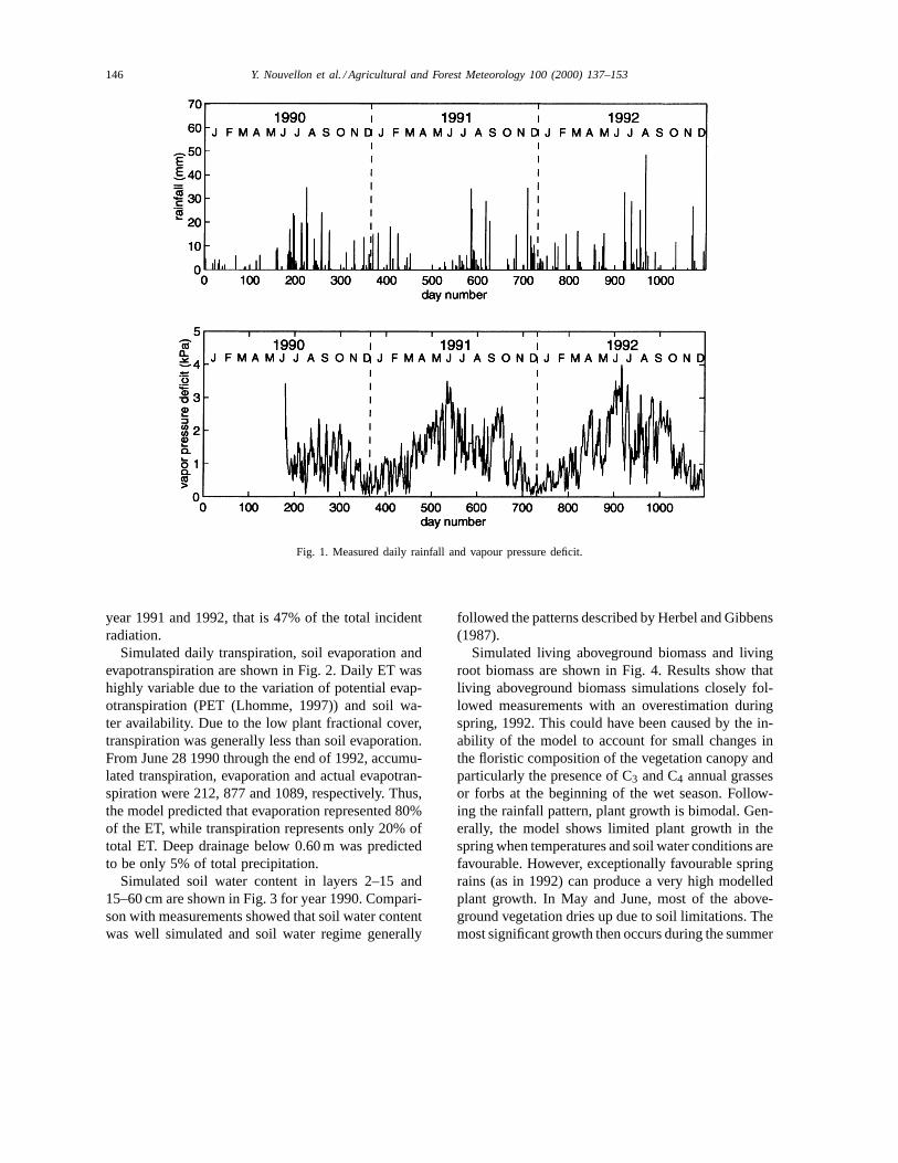
Simulation started before the 1990 monsoon sea-son on June 28 [Day Of Year (DOY) 179] and rancontinuously throughout end of 1992. Daily values ofrainfall and vapour pressure deficit (VPD) are shownon Fig. 1. Annual rainfall amounts were 412, 369 and434 mm for years 1990, 1991 and 1992, respectively(in 1990, 349 mm fell between DOY 179 and 365; seeTable 2). The rainfall patterns are of prime importancefor perennial grass growth and survival. By compar-


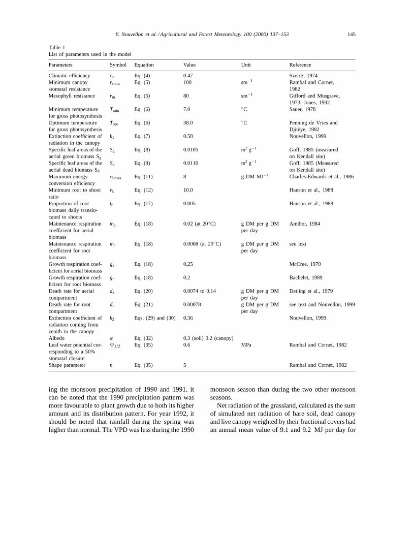
Table 1List of parameters used in the model

Parameters Symbol Equation Value Unit Reference

Climatic efficiency εc Eq. (4) 0.47 Szeicz, 1974Minimum canopystomatal resistance

rsmin Eq. (5) 100 sm−1 Rambal and Cornet,1982

Mesophyll resistance rm Eq. (5) 80 sm−1 Gifford and Musgrave,1973; Jones, 1992

Minimum temperaturefor gross photosynthesis

Tmin Eq. (6) 7.0 ◦C Sauer, 1978

Optimum temperaturefor gross photosynthesis

Topt Eq. (6) 38.0 ◦C Penning de Vries andDjit eye, 1982

Extinction coefficient ofradiation in the canopy

k1 Eq. (7) 0.58 Nouvellon, 1999

Specific leaf areas of theaerial green biomass Sg

Sg Eq. (8) 0.0105 m2 g−1 Goff, 1985 (measuredon Kendall site)

Specific leaf areas of theaerial dead biomass Sd

Sd Eq. (9) 0.0110 m2 g−1 Goff, 1985 (Measuredon Kendall site)

Maximum energyconversion efficiency

εbmax Eq. (11) 8 g DM MJ−1 Charles-Edwards et al., 1986

Minimum root to shootratio

rx Eq. (12) 10.0 Hanson et al., 1988

Proportion of rootbiomass daily translo-cated to shoots

tr Eq. (17) 0.005 Hanson et al., 1988

Maintenance respirationcoefficient for aerialbiomass

ma Eq. (18) 0.02 (at 20◦C) g DM per g DMper day

Amthor, 1984

Maintenance respirationcoefficient for rootbiomass

mr Eq. (18) 0.0008 (at 20◦C) g DM per g DMper day

see text

Growth respiration coef-ficient for aerial biomass

ga Eq. (18) 0.25 McCree, 1970

Growth respiration coef-ficient for root biomass

gr Eq. (18) 0.2 Bachelet, 1989

Death rate for aerialcompartment

da Eq. (20) 0.0074 to 0.14 g DM per g DMper day

Detling et al., 1979

Death rate for rootcompartment

dr Eq. (21) 0.00078 g DM per g DMper day

see text and Nouvellon, 1999

Extinction coefficient ofradiation coming fromzenith in the canopy

k2 Eqs. (29) and (30) 0.36 Nouvellon, 1999

Albedo α Eq. (32) 0.3 (soil) 0.2 (canopy)Leaf water potential cor-responding to a 50%stomatal closure

91/2 Eq. (35) 0.6 MPa Rambal and Cornet, 1982

Shape parameter n Eq. (35) 5 Rambal and Cornet, 1982

ing the monsoon precipitation of 1990 and 1991, itcan be noted that the 1990 precipitation pattern wasmore favourable to plant growth due to both its higheramount and its distribution pattern. For year 1992, itshould be noted that rainfall during the spring washigher than normal. The VPD was less during the 1990

monsoon season than during the two other monsoonseasons.

Net radiation of the grassland, calculated as the sumof simulated net radiation of bare soil, dead canopyand live canopy weighted by their fractional covers hadan annual mean value of 9.1 and 9.2 MJ per day for


Fig. 1. Measured daily rainfall and vapour pressure deficit.

year 1991 and 1992, that is 47% of the total incidentradiation.

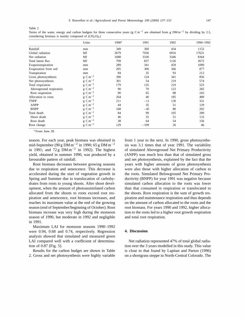
Simulated daily transpiration, soil evaporation andevapotranspiration are shown in Fig. 2. Daily ET washighly variable due to the variation of potential evap-otranspiration (PET (Lhomme, 1997)) and soil wa-ter availability. Due to the low plant fractional cover,transpiration was generally less than soil evaporation.From June 28 1990 through the end of 1992, accumu-lated transpiration, evaporation and actual evapotran-spiration were 212, 877 and 1089, respectively. Thus,the model predicted that evaporation represented 80%of the ET, while transpiration represents only 20% oftotal ET. Deep drainage below 0.60 m was predictedto be only 5% of total precipitation.

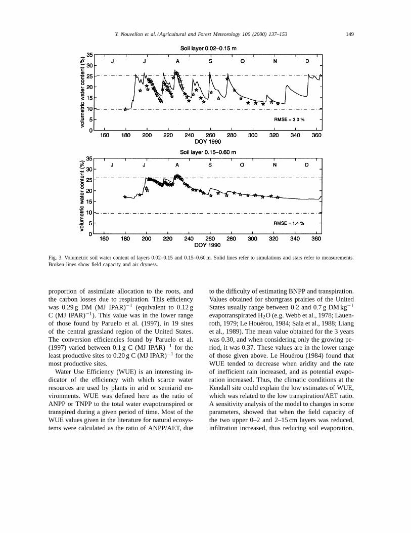
Simulated soil water content in layers 2–15 and15–60 cm are shown in Fig. 3 for year 1990. Compari-son with measurements showed that soil water contentwas well simulated and soil water regime generally

followed the patterns described by Herbel and Gibbens(1987).

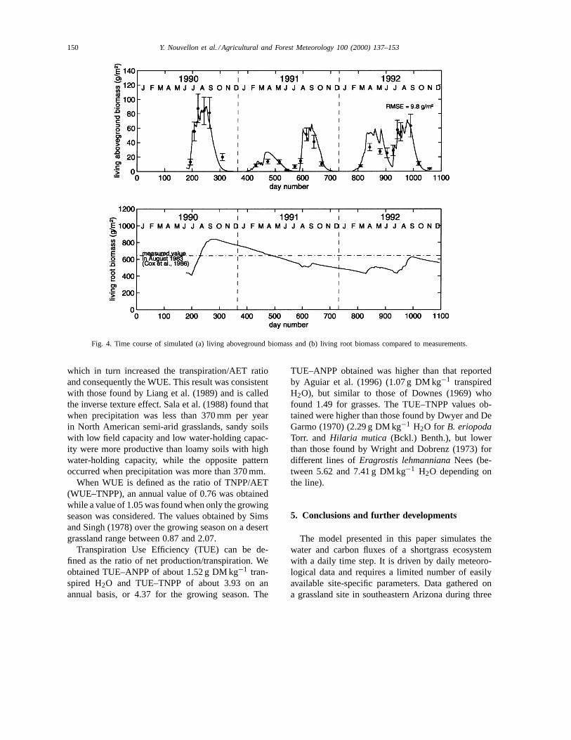
Simulated living aboveground biomass and livingroot biomass are shown in Fig. 4. Results show thatliving aboveground biomass simulations closely fol-lowed measurements with an overestimation duringspring, 1992. This could have been caused by the in-ability of the model to account for small changes inthe floristic composition of the vegetation canopy andparticularly the presence of C3 and C4 annual grassesor forbs at the beginning of the wet season. Follow-ing the rainfall pattern, plant growth is bimodal. Gen-erally, the model shows limited plant growth in thespring when temperatures and soil water conditions arefavourable. However, exceptionally favourable springrains (as in 1992) can produce a very high modelledplant growth. In May and June, most of the above-ground vegetation dries up due to soil limitations. Themost significant growth then occurs during the summer


Table 2Terms of the water, energy and carbon budgets for three consecutive years (g C m−2 are obtained from g DM m−2 by dividing by 2.5,considering biomass is mainly composed of (CH2O)n)

Units 1990a 1991 1992 1990–1992

Rainfall mm 349 369 434 1152Global radiation MJ 3679 7036 6916 17631Net radiation MJ 1688 3330 3346 8364Total latent flux MJ 709 837 1126 2672Evapotranspiration mm 289 341 459 1089Evaporation from soil mm 205 306 366 877Transpiration mm 84 35 93 212Gross photosynthesis g C m−2 390 124 341 856Net photosynthesis g C m−2 301 54 219 574Total respiration g C m−2 179 135 210 525Aboveground respiration g C m−2 90 70 122 282Root respiration g C m−2 90 65 88 243

Allocation to roots g C m−2 264 40 185 489TNPP g C m−2 211 −11 130 331ANPP g C m−2 44 35 51 129BNPP g C m−2 168 −45 80 202

Total death g C m−2 84 99 105 289Shoot death g C m−2 46 35 51 133Root death g C m−2 38 64 54 156

Root change g C m−2 129 −109 26 46

a From June 28.

season. For each year, peak biomass was obtained inmid-September (90 g DM m−2 in 1990; 65 g DM m−2

in 1991; and 72 g DM m−2 in 1992). The highestyield, obtained in summer 1990, was produced by afavourable pattern of rainfall.

Root biomass decreases between growing seasonsdue to respiration and senescence. This decrease isaccelerated during the start of vegetation growth inSpring and Summer due to translocation of carbohy-drates from roots to young shoots. After shoot devel-opment, when the amount of photoassimilated carbonallocated from the shoots to roots exceed root res-piration and senescence, root biomass increases, andreaches its maximum value at the end of the growingseason (end of September/beginning of October). Rootbiomass increase was very high during the monsoonseason of 1990, but moderate in 1992 and negligiblein 1991.

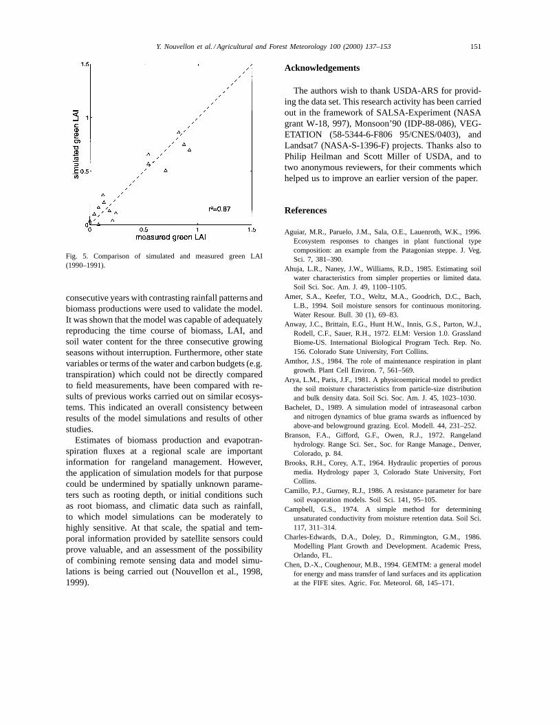
Maximum LAI for monsoon seasons 1990–1992were 0.94, 0.68 and 0.74, respectively. Regressionanalysis showed that simulated and measured greenLAI compared well with a coefficient of determina-tion of 0.87 (Fig. 5).

Results for the carbon budget are shown in Table2. Gross and net photosynthesis were highly variable

from 1 year to the next. In 1990, gross photosynthe-sis was 3.1 times that of year 1991. The variabilityof simulated Aboveground Net Primary Productivity(ANPP) was much less than that of simulated grossand net photosynthesis, explained by the fact that theyears with higher amounts of gross photosynthesiswere also those with higher allocation of carbon tothe roots. Simulated Belowground Net Primary Pro-ductivity (BNPP) for year 1991 was negative becausesimulated carbon allocation to the roots was lowerthan that consumed in respiration or translocated tothe shoots. Root respiration is the sum of growth res-piration and maintenance respiration and thus dependson the amount of carbon allocated to the roots and theroot biomass. For years 1990 and 1992, higher alloca-tion to the roots led to a higher root growth respirationand total root respiration.

4. Discussion

Net radiation represented 47% of total global radia-tion over the 3 years modelled in this study. This valueis close to that found by Lapitan and Parton (1996)on a shortgrass steppe in North-Central Colorado. The


Fig. 2. Simulated daily (a) total evaporation, (b) evaporation from soil, and (c) transpiration.

evaporation processes used on average 32% of the netradiation. The amount of transpiration was found tobe low when compared to evaporation. On an annualbasis, modelled transpiration represented only 20% ofactual evapotranspiration because of the low fractionalcover of green vegetation even during the growing sea-son. Furthermore, this region is often characterised bysmall inefficient rain events that wet only the surfacesoil layer.

Mean annual ANPP and TNPP (Aboveground andTotal Net Primary Productivity) were 107 and 276 gDM m−2, respectively. Thus, the ratio of ANPP/TNPPwas 0.39. For semi-arid grasslands, values for this ra-tio range between 0.25 and 0.6 (Sims and Singh, 1978;Milchunas and Lauenroth, 1992). Over the 3 years,57% of gross photosynthesis and 85% of net photo-synthesis were allocated to roots. This is consistentwith the simulation results of Detling et al. (1979)who found that 65% ofPg and 80% ofPn were allo-

cated to belowground structures. Sixty-one percent ofPg was lost in total respiration, a value close to thatfound by Detling et al. (1979). Root respiration repre-sented 46% of total respiration, an intermediate valuebetween the lowest 21% found by Bachelet (1989) andthe highest 71% by Detling et al. (1979). The amountlost by aboveground respiration was 33% ofPg.

Efficiency of PAR interception by green leaves wasclosely related to the pattern of LAI development.The maximum value was 0.41 for a LAI of 0.94. Overthe simulation period, only 14% of the incident PARwas intercepted by living vegetation. The efficiencywith which this intercepted PAR was converted intogross photosynthesis was 1.92 g DM (MJ IPAR)−1.This simulated low value was due to the effect ofnon-optimum temperatures, water limitation and leafageing. The efficiency with which the intercepted PARwas converted into aboveground net production wasfound to be even lower, due to the model’s high


Fig. 3. Volumetric soil water content of layers 0.02–0.15 and 0.15–0.60 m. Solid lines refer to simulations and stars refer to measurements.Broken lines show field capacity and air dryness.

proportion of assimilate allocation to the roots, andthe carbon losses due to respiration. This efficiencywas 0.29 g DM (MJ IPAR)−1 (equivalent to 0.12 gC (MJ IPAR)−1). This value was in the lower rangeof those found by Paruelo et al. (1997), in 19 sitesof the central grassland region of the United States.The conversion efficiencies found by Paruelo et al.(1997) varied between 0.1 g C (MJ IPAR)−1 for theleast productive sites to 0.20 g C (MJ IPAR)−1 for themost productive sites.

Water Use Efficiency (WUE) is an interesting in-dicator of the efficiency with which scarce waterresources are used by plants in arid or semiarid en-vironments. WUE was defined here as the ratio ofANPP or TNPP to the total water evapotranspired ortranspired during a given period of time. Most of theWUE values given in the literature for natural ecosys-tems were calculated as the ratio of ANPP/AET, due

to the difficulty of estimating BNPP and transpiration.Values obtained for shortgrass prairies of the UnitedStates usually range between 0.2 and 0.7 g DM kg−1

evapotranspirated H2O (e.g. Webb et al., 1978; Lauen-roth, 1979; Le Houérou, 1984; Sala et al., 1988; Lianget al., 1989). The mean value obtained for the 3 yearswas 0.30, and when considering only the growing pe-riod, it was 0.37. These values are in the lower rangeof those given above. Le Houérou (1984) found thatWUE tended to decrease when aridity and the rateof inefficient rain increased, and as potential evapo-ration increased. Thus, the climatic conditions at theKendall site could explain the low estimates of WUE,which was related to the low transpiration/AET ratio.A sensitivity analysis of the model to changes in someparameters, showed that when the field capacity ofthe two upper 0–2 and 2–15 cm layers was reduced,infiltration increased, thus reducing soil evaporation,


Fig. 4. Time course of simulated (a) living aboveground biomass and (b) living root biomass compared to measurements.

which in turn increased the transpiration/AET ratioand consequently the WUE. This result was consistentwith those found by Liang et al. (1989) and is calledthe inverse texture effect. Sala et al. (1988) found thatwhen precipitation was less than 370 mm per yearin North American semi-arid grasslands, sandy soilswith low field capacity and low water-holding capac-ity were more productive than loamy soils with highwater-holding capacity, while the opposite patternoccurred when precipitation was more than 370 mm.

When WUE is defined as the ratio of TNPP/AET(WUE–TNPP), an annual value of 0.76 was obtainedwhile a value of 1.05 was found when only the growingseason was considered. The values obtained by Simsand Singh (1978) over the growing season on a desertgrassland range between 0.87 and 2.07.

Transpiration Use Efficiency (TUE) can be de-fined as the ratio of net production/transpiration. Weobtained TUE–ANPP of about 1.52 g DM kg−1 tran-spired H2O and TUE–TNPP of about 3.93 on anannual basis, or 4.37 for the growing season. The

TUE–ANPP obtained was higher than that reportedby Aguiar et al. (1996) (1.07 g DM kg−1 transpiredH2O), but similar to those of Downes (1969) whofound 1.49 for grasses. The TUE–TNPP values ob-tained were higher than those found by Dwyer and DeGarmo (1970) (2.29 g DM kg−1 H2O for B. eriopodaTorr. andHilaria mutica (Bckl.) Benth.), but lowerthan those found by Wright and Dobrenz (1973) fordifferent lines ofEragrostis lehmannianaNees (be-tween 5.62 and 7.41 g DM kg−1 H2O depending onthe line).

5. Conclusions and further developments

The model presented in this paper simulates thewater and carbon fluxes of a shortgrass ecosystemwith a daily time step. It is driven by daily meteoro-logical data and requires a limited number of easilyavailable site-specific parameters. Data gathered ona grassland site in southeastern Arizona during three


Fig. 5. Comparison of simulated and measured green LAI(1990–1991).

consecutive years with contrasting rainfall patterns andbiomass productions were used to validate the model.It was shown that the model was capable of adequatelyreproducing the time course of biomass, LAI, andsoil water content for the three consecutive growingseasons without interruption. Furthermore, other statevariables or terms of the water and carbon budgets (e.g.transpiration) which could not be directly comparedto field measurements, have been compared with re-sults of previous works carried out on similar ecosys-tems. This indicated an overall consistency betweenresults of the model simulations and results of otherstudies.

Estimates of biomass production and evapotran-spiration fluxes at a regional scale are importantinformation for rangeland management. However,the application of simulation models for that purposecould be undermined by spatially unknown parame-ters such as rooting depth, or initial conditions suchas root biomass, and climatic data such as rainfall,to which model simulations can be moderately tohighly sensitive. At that scale, the spatial and tem-poral information provided by satellite sensors couldprove valuable, and an assessment of the possibilityof combining remote sensing data and model simu-lations is being carried out (Nouvellon et al., 1998,1999).

Acknowledgements

The authors wish to thank USDA-ARS for provid-ing the data set. This research activity has been carriedout in the framework of SALSA-Experiment (NASAgrant W-18, 997), Monsoon’90 (IDP-88-086), VEG-ETATION (58-5344-6-F806 95/CNES/0403), andLandsat7 (NASA-S-1396-F) projects. Thanks also toPhilip Heilman and Scott Miller of USDA, and totwo anonymous reviewers, for their comments whichhelped us to improve an earlier version of the paper.

References

Aguiar, M.R., Paruelo, J.M., Sala, O.E., Lauenroth, W.K., 1996.Ecosystem responses to changes in plant functional typecomposition: an example from the Patagonian steppe. J. Veg.Sci. 7, 381–390.

Ahuja, L.R., Naney, J.W., Williams, R.D., 1985. Estimating soilwater characteristics from simpler properties or limited data.Soil Sci. Soc. Am. J. 49, 1100–1105.

Amer, S.A., Keefer, T.O., Weltz, M.A., Goodrich, D.C., Bach,L.B., 1994. Soil moisture sensors for continuous monitoring.Water Resour. Bull. 30 (1), 69–83.

Anway, J.C., Brittain, E.G., Hunt H.W., Innis, G.S., Parton, W.J.,Rodell, C.F., Sauer, R.H., 1972. ELM: Version 1.0. GrasslandBiome-US. International Biological Program Tech. Rep. No.156. Colorado State University, Fort Collins.

Amthor, J.S., 1984. The role of maintenance respiration in plantgrowth. Plant Cell Environ. 7, 561–569.

Arya, L.M., Paris, J.F., 1981. A physicoempirical model to predictthe soil moisture characteristics from particle-size distributionand bulk density data. Soil Sci. Soc. Am. J. 45, 1023–1030.

Bachelet, D., 1989. A simulation model of intraseasonal carbonand nitrogen dynamics of blue grama swards as influenced byabove-and belowground grazing. Ecol. Modell. 44, 231–252.

Branson, F.A., Gifford, G.F., Owen, R.J., 1972. Rangelandhydrology. Range Sci. Ser., Soc. for Range Manage., Denver,Colorado, p. 84.

Brooks, R.H., Corey, A.T., 1964. Hydraulic properties of porousmedia. Hydrology paper 3, Colorado State University, FortCollins.

Camillo, P.J., Gurney, R.J., 1986. A resistance parameter for baresoil evaporation models. Soil Sci. 141, 95–105.

Campbell, G.S., 1974. A simple method for determiningunsaturated conductivity from moisture retention data. Soil Sci.117, 311–314.

Charles-Edwards, D.A., Doley, D., Rimmington, G.M., 1986.Modelling Plant Growth and Development. Academic Press,Orlando, FL.

Chen, D.-X., Coughenour, M.B., 1994. GEMTM: a general modelfor energy and mass transfer of land surfaces and its applicationat the FIFE sites. Agric. For. Meteorol. 68, 145–171.


Clapp, R.B., Hornberger, G.M., 1978. Empirical equations forsome hydraulic properties. Water Resour. Res. 14, 601–604.

Clark, F.E., Paul, E.A., 1970. The microflora of grassland. Adv.Agron. 22, 375–435.

Coughenour, M.B., McNaughton, S.J., Wallace, L.L., 1984.Modelling primary production of perennial graminoids —uniting physiological processes and morphometric traits. Ecol.Modell. 23, 101–134.

Cox, J.R., Frasier, G.W., Renard, K.G., 1986. Biomass distributionat Grassland and Shrubland sites. Rangelands 8 (2), 67–68.

De Jong, R., 1983. Soil water description curves estimated fromlimited data. Can. J. Soil Sci. 63, 697–703.

Detling, J.K., Parton, W.J., Hunt, H.W., 1979. A simulation modelof Bouteloua gracilisbiomass dynamics on the North Americanshortgrass prairie. Oecologia 38, 167–191.

Downes, R.W., 1969. Differences in transpiration rates betweentropical and temperate grasses under controlled conditions.Planta 88, 261–273.

Dunkerley, D.L., Booth, T.L., 1999. Plant canopy interception ofrainfall and its significance in a banded landscape, arid westernNew South Wales, Australia. Water Resour. Res. 35 (5), 1581–1586.

Dwyer, D.D., De Garmo, H.C., 1970. Greenhouse productivityand water use efficiency of selected desert shrubs and grassesunder four soil-moisture levels New Mexico State University,Agric. Exp. Stat. Bull. 570, Las Cruces, New Mexico.

Feddes, R.A., Kowalik, P.J., Zaradny H., 1978. Simulation of fieldwater use and cropyield. Simulation Monograph. Pudoc-DLO,Wageningen, The Netherlands, p. 189.

Gifford, R.M., Musgrave, R.B., 1973. Stomatal role in thevariability of net CO2 exchange rate by two maize inbreds.Aust. J. Biol. Sci. 26, 35–44.

Goff, B.F., 1985. Dynamics of canopy structure and soil surfacecover in a semi-arid grassland. Master’s thesis, University ofArizona, Tucson.

Goodrich, D.C., 1994. SALSA-MEX: A large scale Semi-AridLand-Surface-Atmospheric Mountain Experiment. In: Proc.Int. Geoscience and Remote Sensing Symp. (IGARSS’94),Pasadena, CA, vol. 1, August 8–12, 1994, pp. 190–193.

Goodrich, D.C., Chehbouni, A.G., Goff, B. et al., 1998.An overview of the 1997 activities of the Semi-AridLand-Surface-Atmosphere (SALSA program). Proc. 78thAmerican Meteorological Society Annual Meeting, Phoenix,Arizona, 11–16 January.

Hanson, J.D., Parton, W.J., Innis, G.S., 1985. Plant growth andproduction of grassland ecosystems: a comparison of modellingapproaches. Ecol. Modell. 29, 131–144.

Hanson, J.D., Skiles, J.W., Parton, W.J., 1988. A multi-speciesmodel for rangeland plant communities. Ecol. Modell. 44, 89–123.

Herbel, C.H., Gibbens, R.P., 1987. Soil water regimes of loamysands and sandy loams on arid rangelands in southern NewMexico. J. Soil Water Conserv. 42, 442–447.

Jones, H.G., 1992. Plants and Microclimate. A QuantitativeApproach to Environmental Plant Physiology, 2nd ed.Cambridge University Press, Cambridge, p. 429.

Kowalik, P.J., Turner, N.C., 1983. Diurnal changes in the waterrelations and transpiration of a soybean crop simulated duringthe development of water deficits. Irrig. Sci. 4, 225–238.

Kustas, W.P., Goodrich, D.C., 1994. Preface to the special issueon Monsoon 90. Water Resour. Res. 30 (5), 1211–1225.

Kustas, W.P., Blanford, J.A., Stannard, D.I., Daughtry, C.S.T.,Nichols, W.D., Weltz, M.A., 1994. Water Resour. Res. 30 (5),1351–1361.

Lapitan, R.L., Parton, W.J., 1996. Seasonal variabilities in thedistribution of the microclimatic factors and evapotranspirationin a shortgrass steppe. Agric. For. Meteorol. 79, 113–130.

Lauenroth, W.K., 1979. Grassland primary production:North American grasslands in perspective. In: French,N.L. (Ed.), Perspectives in Grassland Ecology. Springer,Berlin/Heidelberg/New York, pp. 2–24.

Leenhardt, D., Voltz, M., Rambal, S., 1995. A survey of severalagroclimatic soil water balance models with reference to theirspatial application. Eur. J. Agron. 4, 1–14.

Le Houérou, H.N., 1984. Rain use efficiency: a unifying conceptin arid-land ecology. J. Arid Environ. 7, 213–247.

Liang, Y.M., Hazlett, D.L., Lauenroth, W.K., 1989. Biomassdynamics and water use efficiencies of five plant communitiesin the shortgrass steppe. Oecologia 80, 148–153.

Lhomme, J.P., 1997. Towards a rational definition of potentialevaporation. Hydrol. Earth System Sci. 1 (2), 257–264.

Lo Seen, D., Mougin, E., Rambal, S., Gaston, A., Hiernaux,P., 1995. A regional Sahelian grassland model to be coupledwith multispectral satellite data. II. Toward the control of itssimulations by remotely sensed indices. Remote Sens. Environ.52, 194–206.

Lo Seen, D., Chehbouni, A., Njoku, E., Saatchi, S., Mougin,E., Monteny, B., 1997. An approach to couple vegetationfunctioning and soil-vegetation-atmosphere-transfer models forsemiarid grasslands during the HAPEX-Sahel experiment.Agric. For. Meteorol. 83, 49–74.

McCree, K.J., 1970. An equation for the rate of respiration ofwhite clover plants grown under controlled conditions. In:Setlik, I. (Ed.), Prediction and Measurement of PhotosyntheticProductivity. Proc. IBP/PP Tech. Meet., Trebon. PUDOC,Wageningen, The Netherlands, pp. 221–229.

Mc Mahon, J.A., Wagner, F.H., 1985. The Mojave, Sonoranand Chihuahuan deserts of North America. In: Evenari, M.,Noy-Meir, I., Goodall, D.W. (Eds.), Hot Deserts and AridShrublands. Ecosystems of the world 12A, pp. 105–202.

Milchunas, D.G., Lauenroth, W.K., 1992. Carbon dynamics andestimates of primary production by harvest,14C dilution, and14C turnover. Ecology 73 (2), 593–607.

Monteith, J.L., 1965. Evaporation and the environment. Symp.Soc. Exp. Biol. 19, 205–234.

Mougin, E., Lo Seen, D., Rambal, S., Gaston, A., Hiernaux, P.,1995. A regional Sahelian grassland model to be coupled withmultispectral satellite data. I. Model description and validation.Remote Sens. Environ. 52, 181–193.

Nouvellon, Y., 1999. Modélisation du fonctionnement de prairiessemi-arides et assimilation de données radiométriques dansle modèle. Ph.D. thesis, Institut National AgronomiqueParis-Grignon.


Nouvellon, Y., Lo Seen, D., Bégué, A., Rambal, S., Moran, M.S.,Qi, J., Chehbouni, A., Kerr, Y., 1998. Combining remote sensingand vegetation growth modeling to describe the carbon andwater budget of semi-arid grasslands. IGARSS’98, 6–10 July,Seattle, Washington.

Nouvellon, Y., Lo Seen, D., Rambal, S., Bégué, A., Moran, M.S.,Kerr, Y., Qi, J., 1999. Time course of radiation use efficiencyin a shortgrass ecosystem: consequences for remotely-sensedestimation of primary production. Remote Sens. Environ., inpress.

Osborn, H.B., Lane, L.J., Hundley, J.F., 1972. Optimum gaging ofthunderstorm rainfall in Southeastern Arizona. Water Resour.Res. 8 (1), 259–265.

Paruelo, J.M., Epstein, H.E., Lauenroth, W.K., Burke, I.C., 1997.ANPP estimates from NDVI for the central grassland regionof the United States. Ecology 78 (3), 953–958.

Penning de Vries, F.W.T., Djitèye, M.A., 1982. La productivitédes pâturages Sahéliens. Une étude des sols, des végétations etde l’exploitation de cette ressource naturelle. Agric. Res. Rep.918, Pudoc, Wageningen, p. 525.

Perrin de Brichambaut, C., Vauge, C., 1982. Le gisement solaire.Evaluation de la ressource énergétique. Lavoisier Ed., Paris.

Rambal, S., Cornet, A., 1982. Simulation de l’utilisation de l’eauet de la production végétale d’une phytocénose Sahélienne duSénégal. Acta Oecologica Oecol. Plant 3 (17), 381–397.

Rawls, W.J., Brakensiek, D.L., Saxton, K.E., 1982. Estimation ofsoil water properties. Transac. Am. Soc. Agric. Eng. 25, 1316–1320.

Renard, K.G., Lane, L.J., Simanton, J.R., Emmerich, W.E., Stone,J.J., Weltz, M.A., Goodrich, D.C., Yakowitz, D.S., 1993.Agricultural impacts in an arid environment: Walnut Gulchstudies. Hydrol. Sci. Technol. 9 (1–4), 145–190.

Ruimy, A., Dedieu, G., Saugier, B., 1996. TURC: a diagnosticmodel of continental gross primary productivity and net primaryproductivity. Glob. Biogeochem. Cycles 10, 269–286.

Sala, O.E., Parton, W.J., Joyce, L.A., Lauenroth, W.K., 1988.Primary production of the central grassland region of the UnitedStates. Ecology 69 (1), 40–45.

Sauer, R.H., 1978. A simulation model for grassland primaryproducer phenology and biomass dynamics. In: Innis, G.S.(Ed.), Grassland Simulation Model. Ecological Studies, 26.Springer, Berlin/Heidelberg/New York, pp. 55–87.

Saxton, K.E., Rawls, W.J., Romberger, J.S., Papendick, R.I., 1986.Estimating generalized soil-water characteristics from texture.Soil Sci. Soc. Am. J. 50, 1031–1036.

Sellers, W.D., Hill, R.H., 1974. Arizona climate 1931–1972. TheUniversity of Arizona Press, Tucson.

Sims, P.L., Singh, J.S., 1978. The structure and the function of tenwestern north american grasslands. III. Net primary production.Turnover and efficiencies of energy capture and water use. J.Ecol. 66, 573–597.

Singh, J.S., Coleman, D.C., 1975. Evaluation of functional rootbiomass and translocation of photoassimilated carbon-14 ina shortgrass prairie ecosystem. In: Marshall, J.K. (Ed.), TheBelowground Ecosystem: A Synthesis of Plant AssociatedProcesses. Dowden, Hutchison and Ross, Stroudsburg,Pennsylvania.

Shuttleworth, W.J., 1993. Evaporation. In: Maidment, D.R. (Ed.),Handbook of Hydrology. McGraw-Hill, New York.

Stannard, D.I., Blanford, J.H., Kustas, W.P., Nichols, W.D., Amer,S.A., Schmugge, T.J., Weltz, M.A., 1994. Interpretation ofsurface flux measurements in heterogeneous terrain during theMonsoon ’90 experiment. Water Resour. Res. 30 (5), 1227–1239.

Szeicz, G., 1974. Solar radiation for plant growth. J. Appl. Ecol.11, 617–636.

Tiscareno-Lopez, M., 1994. A bayesian-monte carlo approach toaccess uncertainties in process-based, continuous simulationmodels. Ph.D. thesis, University of Arizona, Tucson.

Thurow, T.L., Blackburn, W.H., Warren, S.D., Taylor, C.A., 1987.Rainfall interception by midgrass, shortgrass, and live oakmottes. J. Range Manage. 40, 455–460.

Van Keulen, H., 1975. Simulation of water use and herbage growthin arid regions. Simulation Monographs. Pudoc, Wageningen,p. 176.

Webb, W., Szarek, S., Lauenroth, W., Kinerson, R., Smith,M., 1978. Primary productivity and water use in nativeforest, grassland, and desert ecosystems. Ecology 59 (6)1239–1247.

Weltz, M.A., Ritchie, J.C., Fox, H.D., 1994. Comparison of laserand field measurements of vegetation height and canopy cover.Water Resour. Res. 30 (5), 1311–1319.

White, E.G., 1984. A multispecies simulation model of grasslandproducers and consumers II. Producers. Ecol. Modell. 24, 241–262.

Wright, L.N., Dobrenz, A.K., 1973. Efficiency of water use andassociated characteristics of Lehmann Lovegrass. J. RangeManage. 26 (3), 210–212.

Modelling of daily fluxes of water and carbon from shortgrass steppes

Documents