Modelling Mortality with Common Stochastic Long-Run Trends

Page 1

Forecasting Mortality Trends allowing forCause-of-Death Mortality Dependence

Severine Gaille1 Michael Sherris2

Abstract

Longevity risk is amongst the most important factors to consider for pric-ing and risk management of longevity products. Past improvements in mor-tality over many years, and the uncertainty of these improvements, haveattracted the attention of experts, both practitioners and academics. Sinceaggregate mortality rates reflect underlying trends in causes of death, insurersand demographers are increasingly considering cause-of-death data to betterunderstand risks in their mortality assumptions. The relative importance ofcauses of death has changed over many years. As one cause reduces, othersincrease or decrease. The dependence between mortality for different causesof death is important when projecting future mortality. However, for sce-nario analysis based on causes of death, the assumption usually made is thatcauses of death are independent. Recent models, in the form of Vector ErrorCorrection Models (VECM), have been developed for multivariate dynamicsystems and capture time dependency with common stochastic trends. Thesemodels include long-run stationary relations between the variables, and thusallow a better understanding of the nature of this dependence. This paperapplies VECM to cause-of-death mortality rates in order to assess the de-pendence between these competing risks. We analyze the five main causes ofdeath in Switzerland. Our analysis confirms the existence of a long-run sta-tionary relationship between these five causes. This estimated relationship isthen used to forecast mortality rates, which are shown to be an improvementover forecasts from more traditional ARIMA processes, that do not allow forcause-of-death dependencies.

Keywords: Mortality forecasts, Causes of death, VECM, Dependence, CommontrendsJEL Classifications: C32, C52, J11, G22, I13

1Professor of Actuarial ScienceDepartment of Actuarial Science, Faculty of Business and Economics, University of Lausanne,Switzerland, Tel +41 21 692 33 72, [email protected]

2Professor of Actuarial Studies and Chief Investigator ARC Centre of Excellence in PopulationAgeing ResearchMBA, FIAA, FIA, FSA, FFinRisk and Actuarial Studies, CEPAR, Australian School of Business, University of New SouthWales, Australia, Tel +61-2-9385 2333, Fax +61-2-9385 1883, [email protected]

1

Page 2

1 Introduction

Cause-of-death trends have important implications for forecasting aggregate mor-tality rates. The need for better methods of forecasting mortality trends includingthe impact of cause-of-death trends has been recognised for some time (Stoto andDurch, 1993). Official projections in some countries are based on cause-specificmortality, with each cause forecasted in isolation and subsequently aggregated toproduce total mortality (Wong-Fupuy and Haberman (2004)). An important limita-tion is allowing for dependence between cause-of-death mortality rates. Dependencebetween several causes is not observable. For any given death, it is not possible toknow what would have been the future cause of death if the person had remainedalive. Therefore, the common assumption is that of independence between causesof death, following early work of Chiang (1968).

A better understanding of trends in the underlying causes of death has thepotential to improve mortality projections. The use of cause-of-death data is seenas being beneficial (Tuljapurkar (1998), Gutterman and Vanderhoof (1998) andTabeau et al. (2001)) as well as having limitations (Booth and Tickle (2008) andRichards (2009)). Despite this potential, most mortality projections are based onaggregate rates (Pitacco (2004), Booth and Tickle (2008)) or assume independencebetween causes (Andreev and Vaupel (2006)).

There are a number of studies that consider cause-of-death forecasts using the in-dependence assumption including Rogers and Gard (1991), Wilmoth (1996), Tabeauet al. (1999), Caselli et al. (2006). In these studies, total future mortality rate re-sults from the summation of cause-specific mortality forecasts, each cause beingprojected without taking into account trends in other causes of death. For exam-ple, in McNown and Rogers (1992), univariate ARIMA models are used to forecastparameters of a function fitted to the age pattern of mortality. They forecast thefour main causes of death (heart diseases, cancer, vascular diseases, accident andviolence) and other causes to 1985 using data from 1960 to 1975. A similar approachis used in Knudsen and McNown (1993). Caselli (1996) forecasts mortality by causefor ages 60 and over for 25 European countries over the period 1988-2020, using datafrom 1950 to 1990 and an Age-Period-Cohort model. She adds cause-specific ratesto estimate future aggregate mortality rates.

In this paper, we propose an approach for capturing the dependence betweencauses of death using Vector Autoregression (VAR) and Vector Error CorrectionModels (VECM). They have been developed in econometrics to model multivari-ate dynamic systems including time dependency between economic variables andallowing for common stochastic trends. VECM also include long-run equilibriumrelationships using cointegrating relations. We apply VECM to cause-of-death mor-tality rates. The analysis supports the existence of long-run stationary relationshipsbetween the five main causes of death and provides insights into the form of depen-dence between these competing risks over recent years. These long-run stationaryrelationships are then used to forecast mortality rates. The benefits gained frommodeling the underlying cause trends with these methods are quantified by com-paring the resulting mortality forecasts with those from more traditional ARIMAprocesses, that do not allow for cause-of-death dependencies.

This paper presents a new modeling approach for researchers interested in un-derstanding the dependence between cause-of-death mortality rates. The model-

2

Page 3

ing approach provides the potential to assist practitioners in setting dependenceassumptions for scenario analysis based on cause-of-death mortality. The bene-fits of incorporating cause dependence in longevity and mortality risk models aredemonstrated and can be used in official projections for countries interested incause-specific mortality as well as by insurers issuing longevity and mortality riskproducts.

The paper starts with introducing the data in Section 2. After a brief expla-nation of the features of VAR and VECM modeling, these models are applied tocause-specific mortality for females in Switzerland (Section 3). In Section 4, theestimated relationships between the causes of death are used to forecast mortalityrates and the results are compared with forecasts from more traditional ARIMAprocesses. Finally, Section 5 concludes.

2 Data

The World Health Organization (WHO) provides a comprehensive database forcauses of death (World Health Organization (2012)). Mid-year population andnumber of deaths according to the underlying cause of death are maintained forvarious countries over the last 50 to 60 years. The data are typically divided intofive-year age groups. We use data for Switzerland from 1951 to 2007 to illustratethe methods. Similar benefits would apply to other countries experiencing changesin causes of death.

The WHO database classifies the causes of death according to the InternationalClassification of Diseases (ICD), thus ensuring consistencies between countries (Ta-ble (1)). Under the ICD, the underlying cause of death is specified as the diseaseor injury which initiated the train of morbid events leading directly to death, orthe circumstances of the accident or violence which produced the fatal injury. Inthis study, only the five main ICD primary causes of death are considered, whichare the diseases of the circulatory system, cancer, diseases of the respiratory sys-tem, external causes, and infectious and parasitic diseases. These major causes ofdeath account for about 80% of the deaths in recent years, while they made upapproximately 60% – 70% 50 years ago.

In order to work on data consistent over time and across countries1, a few ad-justments are made to the dataset. First, as recommended by the Human MortalityDatabase (Human Mortality Database (2012)), the number of deaths of unknownage is divided up across the age range.

Second, ages 85 and over are grouped together as well as ages one to four. Thus,our database is composed of nineteen age groups, the first for infants less than oneyear old, a second for children aged one to four, thereafter in groups of five years,ending with the group aged 85 and above.

Third, an adaptation is due to the changes of the classification of the diseasesover time. Indeed, to improve the classification and to adapt it to changes inscience and technology, the ICD evolved from ICD 7 in the 1950’s to ICD 10 stillused today. Therefore, the data are not directly comparable for different periodsand comparability ratios are necessary to allow comparisons, as in Gaille and Sherris(2011). Since Switzerland did not adopt ICD 9, two sets of ratios are developed,

1Future researches might be interested in comparisons across countries.

3

Page 4

one for 1969 when ICD 8 was adopted and one for 1995 when ICD 10 was adopted.By dividing the death number in a new classification with the comparability ratiolinking this classification with the previous one (and previous comparability ratioswhere appropriate), we remove discontinuities in the death rates in 1969 and 1995.Indeed, the comparability ratios are determined so that the average of the deathrates over the last two years of a classification coincides with the average of thedeath rates over the first two years of the next classification (for details, see Gailleand Sherris (2011)).

Finally, trends by cause of death are examined using an age-standardized centraldeath rate, the standard population being equal to the population of the last yearunder observation, here 2007. We denote by m∗

t,d,s the death rate in year t for caused and gender s, assuming that the age-structure of the population is constant overthe complete period under observation and fixed at the level of 2007.

3 Model Fit

Vector AutoRegressive (VAR) models are used to model vectors of variables that areassumed stationary. A pth-order vector autoregression, denoted as VAR(p), is basedon p lags of the variables in the model. Thus, expected changes are modeled byallowing for lagged relationships between the variables and also for the correlationsbetween the variables. For mortality modeling, a vector of age-standardized cause-specific death rates transformed to stationary variables can be effectively modeledwith a VAR.

More efficient processes exist to model non-stationary or integrated variables.These models are called Vector Error Correction Models (VECM). The intuition be-hind these models is that the variables may move together with common stochastictrends, even though they are non-stationary. Therefore, even if each variable is non-stationary, a linear combination of these variables may exist such that the relation isstationary. This linear combination represents a long-run equilibrium relationshipcalled cointegration.2 The system may have more than one cointegrating relation,if each combination is linearly independent from the others. These relations may beincluded in a VAR model, which is then called a VECM. Comprehensive referenceson these models are e.g. Hamilton (1994) and Lutkepohl (2005).

Johansen’s approach is used to estimate the number of cointegrating relations inthe process as well as the parameters of the VECM. The steps to follow to estimatea VECM are summarized in Gaille and Sherris (2011). First, the lag order ofthe VAR is selected through Akaike’s Information Criteria (AIC), Hannan-QuinnCriterion (HQ), Schwarz Criterion (SC), Final Prediction Error (FPE). Second,the stationarity of the variables is considered through several unit root tests: theKwiatkowski-Phillips-Schmidt-Shin test (KPSS), the Augmented Dickey-Fuller test(ADF), the Phillips-Perron test (PP) or the Elliot-Rothenberg-Stock test (ERS).Third, the Johansen’s procedure is applied if some of the variables are integratedin order to find the number of cointegrating relations. For that purpose, the tracetest and the maximum-eigenvalue test are used. Besides, the Johansen’s procedureallows to include a vector of constants and/or a vector of trends in the model while

2In this paper, we consider variables that are integrated of order one. In that special case,cointegrating relations are necessarily stationary. For a more general framework, see Hamilton(1994) and Lutkepohl (2005).

4

Page 5

testing for cointegration. Therefore, depending on the specification of the model, thecointegrating relations may be stationary around a constant level or a trend. Forth,a VAR(p− 1) on the first difference is estimated when the variables are integratedand not cointegrated. Otherwise, the appropriate VECM is developed. Finally,model validation tests should be performed, such as tests for residual autocorrelationand non-normality.

This procedure is applied to cause-specific death rates for females in Switzerland,determined as the logarithm of m∗

t,d,female. The variables of the VECM analysis arethe age-standardized death rates for: 1) diseases of the circulatory system; 2) cancer;3) diseases of the respiratory system; 4) external causes; 5) infectious & parasiticdiseases. Since at least 50 years of observation are usually necessary to reliablyestimate a VECM, the model is fitted over the period 1951 to 2000 and forecastsare performed until 2007. Some details of tests performed are omitted for ease ofpresentation and are available from the authors upon request.

Lag order: The four tests show some contradictory results. FPE indicates a lagorder of two as optimal (a trend and a constant being included in the VAR or not),while SC indicates a lag order of one, AIC a lag order of five and HQ a lag varyingbetween one and two, the result depending on the deterministic part included inthe VAR (a trend, a constant or none). Since this study focuses on forecastingperformances and such performances may be improved with a smaller number ofparameters, a lag of one is adopted.

Unit root tests: The four tests clearly indicate at a 5% significance level that thediseases of the circulatory system, the external causes of death and the infectiousand parasitic diseases are non-stationary. The results are not so evident for theother two causes of death. Indeed, KPSS accepts the null hypothesis of stationarityaround a trend for cancer, while ADF, PP and ERS tests accept the null hypoth-esis of non-stationarity at a 5% significance level. With respect to the diseases ofthe respiratory system, KPSS, ADF and ERS indicate non-stationarity at a 5%significance level, while PP test rejects the non-stationarity. Since three tests outof four point out non-stationarity for these last two causes of death, the five causesof death are assumed non-stationary for the following analysis.

Cointegrating relations: The trace test and the maximum-eigenvalue test ofthe Johansen’s procedure are performed and presented in Table 2. According tothese tests, one cointegrating relation exists between the stochastic death rates ofthe five main causes of death for females in Switzerland. Indeed, the trace statistictests the null hypothesis of r cointegrating relations against the alternative of ncointegarting relations, n being the number of variables in the VECM, here thefive causes of death, and r < n. The test indicates that four, three, two and onecointegrating relations are not rejected against the alternative of five cointegratingrelations at a 5% significance level.

The maximum-eigenvalue statistic tests the null hypothesis of r cointegratingrelations against the alternative of r + 1. Therefore, the null hypothesis of onecointegrating relation is accepted against the alternative of two cointegrating rela-tions, while the null hypothesis of zero cointegrating relation is rejected. Thus, one

5

Page 6

long-run equilibrium relationship ties the causes of death together and reveals howthe death rates were changing relative to each others over the past 50 years.

The Johansen’s approach also allows to test for a potential trend in cointegra-tion. The null hypothesis of no linear trend in cointegration is rejected with ap-value of 0.5%, which indicates that a deterministic trend should be also includedin the cointegrating relation and not only in the variables. In other words, thedeterministic trend is not eliminated by the cointegrating relation. The cointegrat-ing relation represents a stationary process added to a deterministic linear trend.Finally, the null hypothesis of no quadratic trend is accepted at a 2.5% significancelevel, with a p-value close to 4%.

Fitted VECM: The Vector Error Correction Model fitted to the five cause-specific death rates is presented in Equation 1.

∇ logm∗t,I&P,s

∇ logm∗t,cancer,s

∇ logm∗t,circ,s

∇ logm∗t,resp,s

∇ logm∗t,external,s

=

1.29−0.91−3.96−34.72

0.48

+

0.0089−0.0061−0.0265−0.2332

0.0033

×

[1.49 −19.56 −6.32 −4.52 1.86 −0.24

]

×

logm∗t−1,I&P,s

logm∗t−1,cancer,s

logm∗t−1,circ,s

logm∗t−1,resp,s

logm∗t−1,external,s

t− 1

. (1)

The cointegrating relation between the causes of death is given by the secondterm on the right-hand side of this equation. It can be written as

zt = 1.49 · logm∗t−1,I&P,s − 19.56 · logm∗

t−1,cancer,s − 6.32 · logm∗t−1,circ,s

− 4.52 · logm∗t−1,resp,s + 1.86 · logm∗

t−1,external,s − 0.24 · (t− 1), (2)

where zt is a stochastic and stationary variable representing the deviation from theequilibrium. Thus, the model allows for stochastic trends in mortality rates, whilemaintaining long-run relationship between the causes of death through Equation2. Relative changes in mortality between causes are reflected in this relationship,which represents historical evolutions. Mortality was evolving stochastically, butdeath rates were also driven by this long-run equilibrium relationship between thecauses which was maintained stationary over the past 50 years. Thus, by usingsuch a long-run stationary relation in a VECM for forecasting, we assume that thisrelation will continue in the future.

Model validation: Diagnostic tests are performed on the residuals of the fittedmodel. As indicated in Table 3, the normality of the residuals is accepted by thethree tests. However, some autocorrelations between the residuals remain accordingto the Portmanteau test. Such a result is not surprising since we fitted a modelwith a small number of parameters with a lag value of one. A VECM of higher

6

Page 7

order may provide better results with respect to this test. Since we are interested inthe forecasting performance of the model, this is expected to be better with fewerparameters.

4 Forecasting

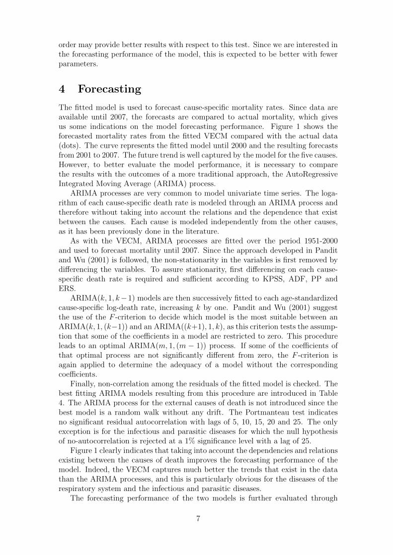
The fitted model is used to forecast cause-specific mortality rates. Since data areavailable until 2007, the forecasts are compared to actual mortality, which givesus some indications on the model forecasting performance. Figure 1 shows theforecasted mortality rates from the fitted VECM compared with the actual data(dots). The curve represents the fitted model until 2000 and the resulting forecastsfrom 2001 to 2007. The future trend is well captured by the model for the five causes.However, to better evaluate the model performance, it is necessary to comparethe results with the outcomes of a more traditional approach, the AutoRegressiveIntegrated Moving Average (ARIMA) process.

ARIMA processes are very common to model univariate time series. The loga-rithm of each cause-specific death rate is modeled through an ARIMA process andtherefore without taking into account the relations and the dependence that existbetween the causes. Each cause is modeled independently from the other causes,as it has been previously done in the literature.

As with the VECM, ARIMA processes are fitted over the period 1951-2000and used to forecast mortality until 2007. Since the approach developed in Panditand Wu (2001) is followed, the non-stationarity in the variables is first removed bydifferencing the variables. To assure stationarity, first differencing on each cause-specific death rate is required and sufficient according to KPSS, ADF, PP andERS.

ARIMA(k, 1, k−1) models are then successively fitted to each age-standardizedcause-specific log-death rate, increasing k by one. Pandit and Wu (2001) suggestthe use of the F -criterion to decide which model is the most suitable between anARIMA(k, 1, (k−1)) and an ARIMA((k+1), 1, k), as this criterion tests the assump-tion that some of the coefficients in a model are restricted to zero. This procedureleads to an optimal ARIMA(m, 1, (m − 1)) process. If some of the coefficients ofthat optimal process are not significantly different from zero, the F -criterion isagain applied to determine the adequacy of a model without the correspondingcoefficients.

Finally, non-correlation among the residuals of the fitted model is checked. Thebest fitting ARIMA models resulting from this procedure are introduced in Table4. The ARIMA process for the external causes of death is not introduced since thebest model is a random walk without any drift. The Portmanteau test indicatesno significant residual autocorrelation with lags of 5, 10, 15, 20 and 25. The onlyexception is for the infectious and parasitic diseases for which the null hypothesisof no-autocorrelation is rejected at a 1% significance level with a lag of 25.

Figure 1 clearly indicates that taking into account the dependencies and relationsexisting between the causes of death improves the forecasting performance of themodel. Indeed, the VECM captures much better the trends that exist in the datathan the ARIMA processes, and this is particularly obvious for the diseases of therespiratory system and the infectious and parasitic diseases.

The forecasting performance of the two models is further evaluated through

7

Page 8

two summary statistics. The first one is the well-known mean absolute percentageerror statistic (MAPE), the average of the absolute percentage gap between theforecasted and observed death rates. The average is made for a specific year overthe five causes.

The second statistic compares the forecasted death rates with the no-changeforecast. The no-change forecast assumes that the future mortality is constant overtime and fixed at the level of the last observation, here the death rates of 2000. Themean square error (MSE) between the forecasted and the observed death rates isdivided by the MSE between the no-change forecast and the observed death rates.The square root of the result represents our second statistic called the no-changeforecast statistic. The MSE are computed over the five causes of death. A modelperforms better than the standard assumption of no change in mortality if the ratiois smaller than unity. Table 5 compares the results for the VECM and ARIMAmodels.

The forecasts of the VECM are much closer to the actual death rates than theforecasts of the ARIMA processes. Indeed, both the MAPE and the no-changeforecast statistics are smaller for the VECM. Besides, since the value of the no-change forecast statistic is below unity, the two models perform better than thestandard assumption of no change in mortality over the seven years.

Since the forecasted trend of the ARIMA process for the diseases of the respi-ratory system and the infectious and parasitic diseases is far from what is actuallyobserved (see Figure 1), these two causes significantly affect the value of the MAPEand the no-change forecast statistics. For these two causes of death, the best as-sumption with an ARIMA process would be that there is no trend and thus, thatmortality is constant over time. Under such an assumption, while keeping theARIMA models described in Table 4 for the three other causes of death, the MAPEand the no-change forecast statistics are reduced, as presented in Table 5 underthe adapted ARIMA, but still higher than the VECM results. Indeed, the VECMperformance comes from its ability to capture relationships between the causes ofdeath and to use them in the forecasting process, while the ARIMA models simplyignore these.

5 Conclusion

This paper presents a new application of VECM to cause-of-death mortality andintroduces a new modeling approach for cause-specific mortality that takes into ac-count dependencies between causes. The model is able to capture long-run trendsand the stationary relationships between the variables. A long-run equilibrium re-lationship is shown to exist between the five main causes of death for Swiss females,providing an approach to model the cause-of-death dependence. By including thisequilibrium relationship, that is the cointegrating relation, in the modeling frame-work, forecasting is shown to be improved. If past trends are expected to continue inthe future, including them in the model instead of modeling each cause in isolation,such as with traditional ARIMA processes, assists in forecasting future mortalityrates.

8

Page 9

References

Andreev, K. F. and Vaupel, J. W. (2006). Forecasts of cohort mortality after age50. Working paper of the Max Planck Institute for Demographic Research.

Booth, H. and Tickle, L. (2008). Mortality modelling and forecasting: A review ofmethods. Annals of Actuarial Science, 3, 3–43.

Caselli, G. (1996). Future longevity among the elderly. In G. Caselli and A. D.Lopez, editors, Health and Mortality among Elderly Populations , pages 235–265.Clarendon Press Oxford.

Caselli, G., Vallin, J., and Marsili, M. (2006). How useful are the causes of deathwhen extrapolating mortality trends. An update. Social Insurance Studies fromthe Swedish Social Insurance, 4.

Chiang, C. L. (1968). Introduction to Stochastic Process in Biostatistics . JohnWiley and Sons, New York.

Gaille, S. and Sherris, M. (2011). Modeling mortality with common stochastic long-run trends. The Geneva Papers on Risk and Insurance - Issues and Practice,36(4), 595–621.

Gutterman, S. and Vanderhoof, I. T. (1998). Forecasting changes in mortality: Asearch for a law of causes and effects. North American Actuarial Journal , 2(4),135–138.

Hamilton, J. D. (1994). Time Series Analysis . Princeton University Press.

Human Mortality Database (2012). University of California, Berkeley (USA), andMax Planck Institute for Demographic Research (Germany). Available at www.

mortality.org or www.humanmortality.de.

Knudsen, C. and McNown, R. (1993). Changing causes of death and the sex differ-ential in the usa: Recent trends and projections. Population Research and PolicyReview , 12, 27–41.

Lutkepohl, H. (2005). New Introduction to Multiple Time Series Analysis . CrownPublishing Group.

McNown, R. and Rogers, A. (1992). Forecasting cause-specific mortality using timeseries methods. International Journal of Forecasting , 8, 413–432.

Pandit, S. M. and Wu, S.-M. (2001). Time Series and System Analysis with Appli-cations . Krieger.

Pitacco, E. (2004). Survival models in a dynamic context: a survey. Insurance:Mathematics and Economics , 35, 279–298.

Richards, S. J. (2009). Selected issues in modelling mortality by cause and in smallpopulations. British Actuarial Journal , 15, 267–283.

Rogers, A. and Gard, K. (1991). Applications of the Heligman/Pollard modelmortality schedule. Population Bulletin of the United Nations , 30, 79–105.

9

Page 10

Stoto, M. A. and Durch, J. S. (1993). Forecasting survival, health, and disability:Report on a workshop. Population and Development Review , 19(3), 557–581.

Tabeau, E., Ekamper, P., Huisman, C., and Bosch, A. (1999). Improving over-all mortality forecasts by analysing cause-of-death, period and cohort effects intrends. European Journal of Population, 15, 153–183.

Tabeau, E., Van Den Bergh Jeths, A., and Heathcote, C. (2001). Forecasting Mor-tality in Developed Countries. Insights from a Statistical, Demographic and Epi-demiological Perspective. Kluwer Academic Publishers, Dordrecht.

Tuljapurkar, S. (1998). Forecasting mortality change: Questions and assumptions.North American Actuarial Journal , 2(4), 127–134.

Wilmoth, J. R. (1996). Mortality projections for Japan: A comparison of fourmethods. In G. Caselli and A. D. Lopez, editors, Health and Mortality amongElderly Populations , pages 266–287. Clarendon Press Oxford.

Wong-Fupuy, C. and Haberman, S. (2004). Projecting mortality trends: Recentdevelopments in the United Kingdom and the United States. North AmericanActuarial Journal , 8(2), 56–83.

World Health Organization (2012). WHO Mortality Database. http://www.who.

int/whosis/mort/download/en/index.html.

10

Page 11

Table 1: International Classification of Diseases - Coding system

Notes: The International Classification of Diseases changed three times between 1951 and 2007.

The aim of these changes was to account for progresses in science and technology and to achieve

more refined descriptions.

11

Page 12

Table 2: Tests for the number of cointegrating relations

(a) Trace test

(b) Maximum-eigenvalue test

Notes: A statistic lower than the corresponding critical value indicates that the null hypothesis

of r cointegrating relations is accepted against the alternative of n (trace test) or the alternative

of r+1 (maximum-eigenvalue test) at a α% significance level. Thus, these tables indicate that one

cointegrating relation is accepted at a 5% significance level. These two tests assess the number

of long-run equilibrium relationships among the age-standardized log-death rates of the five main

causes of death for females in Switzerland over the period 1951–2000.

Table 3: Tests on residuals of the fitted VECM, 1951–2000, females in Switzerland

Notes: The null hypothesis of no-autocorrelation among the residuals is tested through the

Portmanteau statistic, with a lag of 15 and 25. The skewness statistic, the kurtosis statistic and

a combination of these are used to test the normality of the residuals.

12

Page 13

●●

●●●●●

●

●

●

●

●●

●

●●

●

●●●

●

●●

●●●

●●

●●

●●

●

●

●●

●●

●●

●

●●

●●

●●

●●

●

●

●●

●●

●●

1950 1960 1970 1980 1990 2000

−5.

8−

5.6

−5.

4−

5.2

−5.

0−

4.8

years

Circ

ulat

ory

(a) Circulatory

system, VECM

●●

●●●●●

●

●

●

●

●●

●

●●

●

●●●

●

●●

●●●

●●

●●

●●

●

●

●●

●●

●●

●

●●

●●

●●

●●

●

●

●●

●●

●●

1950 1960 1970 1980 1990 2000

−5.

8−

5.6

−5.

4−

5.2

−5.

0−

4.8

years

Circ

ulat

ory

(b) Circulatory

system, ARIMA

●

●

●

●●

●●●

●

●

●

●

●

●●

●

●

●

●●

●

●

●

●●

●●

●

●●

●

●

●●●

●●

●

●

●●

●

●

●

●

●●

●

●

●

●●●

●

●

●●

1950 1960 1970 1980 1990 2000

−6.

1−

6.0

−5.

9−

5.8

years

Can

cer

(c) Cancer, VECM

●

●

●

●●

●●●

●

●

●

●

●

●●

●

●

●

●●

●

●

●

●●

●●

●

●●

●

●

●●●

●●

●

●

●●

●

●

●

●

●●

●

●

●

●●●

●

●

●●

1950 1960 1970 1980 1990 2000

−6.

1−

6.0

−5.

9−

5.8

years

Can

cer

(d) Cancer, ARIMA

●

●

●

●

●

●

●

●

●

●

●

●

●

●

●

●

●

●

●

●

●

●

●

●

●

●

●

●

●

●

●

●

●

●

●

●

●

●●

●

●

●

●

●

●●

●●●

●

●

●●

●

●

●●

1950 1960 1970 1980 1990 2000

−8.

0−

7.5

−7.

0−

6.5

years

Res

pira

tory

(e) Respiratory

system, VECM

●

●

●

●

●

●

●

●

●

●

●

●

●

●

●

●

●

●

●

●

●

●

●

●

●

●

●

●

●

●

●

●

●

●

●

●

●

●●

●

●

●

●

●

●●

●●●

●

●

●●

●

●

●●

1950 1960 1970 1980 1990 2000

−8.

0−

7.5

−7.

0−

6.5

years

Res

pira

tory

(f) Respiratory

system, ARIMA

●

●

●

●

●

●

●

●●

●

●

●

●

●●

●

●●

●

●

●

●

●●

●

●●

●

●●

●●

●

●

●

●

●

●●●

●

●

●

●

●

●

●

●●

●

●

●

●

●

●

●

●

1950 1960 1970 1980 1990 2000

−7.

6−

7.5

−7.

4−

7.3

−7.

2−

7.1

−7.

0

years

Ext

erna

l

(g) External causes,

VECM

●

●

●

●

●

●

●

●●

●

●

●

●

●●

●

●●

●

●

●

●

●●

●

●●

●

●●

●●

●

●

●

●

●

●●●

●

●

●

●

●

●

●

●●

●

●

●

●

●

●

●

●

1950 1960 1970 1980 1990 2000

−7.

6−

7.5

−7.

4−

7.3

−7.

2−

7.1

−7.

0

years

Ext

erna

l(h) External causes,

ARIMA

●

●

●●●

●●

●●

●

●

●●●

●

●

●●

●

●

●●●

●

●●

●

●

●

●

●

●●

●●

●

●

●

●●

●

●

●●

●

●●

●

●

●

●●

●

●●

●●

1950 1960 1970 1980 1990 2000

−9.

5−

9.0

−8.

5−

8.0

years

I&P

(i) Infectious & para-

sitic diseases, VECM

●

●

●●●

●●

●●

●

●

●●●

●

●

●●

●

●

●●●

●

●●

●

●

●

●

●

●●

●●

●

●

●

●●

●

●

●●

●

●●

●

●

●

●●

●

●●

●●

1950 1960 1970 1980 1990 2000

−9.

5−

9.0

−8.

5−

8.0

years

I&P

(j) Infectious & para-

sitic diseases, ARIMA

Figure 1: Observed, fitted and forecasted cause-specific log-death rates, females in

Switzerland

Notes: The observed age-standardized log-death rates are depicted by the dots. The curve

represents the fitted model until 2000 and the forecasted rates since then.

13

Page 14

Table 4: Fitted ARIMA(p, 1, q) processes to the logarithm of m∗t,d,female, Switzerland

Circ: ARIMA(2,1,0) Cancer: ARIMA(1,1,0)

Values CI 95% Values CI 95%

constant -0.017 -0.023 -0.012 -0.006 -0.010 -0.002

trend - - - - - -

φ1 -1.073 -1.477 -0.668 -0.380 -0.647 -0.113

φ2 -0.537 -0.786 -0.287 - - -

θ1 0.517 0.081 0.954 - - -∑ε2t 0.057 0.023

Resp: ARIMA(2,1,0) I&P: ARIMA(0,1,0)

Values CI 95% Values CI 95%

constant -0.059 -0.104 -0.014 -0.098 -0.174 -0.022

trend 0.002 0.000 0.003 0.003 0.000 0.005

φ1 -0.942 -1.166 -0.719 - - -

φ2 -0.609 -0.833 -0.385 - - -

θ1 - - - - - -∑ε2t 1.804 0.871

Notes: All models are identified and estimated over the period 1951 - 2000. First differencing

transformation is performed on every variable.

14

Page 15

Table 5: Mean absolute percentage error and no-change forecast statistics

Notes: The mean absolute percentage error is written as MAPE. The no-change forecast repre-

sents the square root of the ratio of the mean square error of one of the two considered models with

the mean square error of the no-change forecast. The no-change forecast assumes the mortality

does not change anymore and so is fixed at the level of 2000 for the following seven years. All

summary statistics are averages over the five causes of death for females in Switzerland.

Original ARIMA: the statistics result from the ARIMA processes described in Table 4.

Adapted ARIMA: the statistics result from the ARIMA processes described in Table 4, except

for the diseases of the respiratory system and the infectious and parasitic diseases for which the

trend was removed.

15