Modelling microscale flow and colloid transport in saturated porous media

Modeling microscale flow and colloid transport in saturatedporous media

Hui Gao a, Jie Han b, Yan Jin b, and Lian-Ping Wang a,∗aDepartment of Mechanical Engineering, University of Delaware, Newark, DE 19716-3140, USAbDepartment of Plant and Soil Sciences, University of Delaware, Newark, DE 19716-3140, USA

Abstract

The microscale flow of water in natural soil porous media affects the transport of colloids and other con-taminants contained in groundwater. In this study, two completely different computational approaches areapplied to simulate pore-scale viscous flows in saturated porous media. The first is the lattice Boltzmannmethod based on the mesoscopic lattice Boltzmann equation. The second method, referred to as Physalis byits developers, is a hybrid representation in which a numerical solution based on discretized Navier-Stokesequation is coupled with analytical Stokes flow solutions valid locally near the surface of porous-mediumgrains. The porous medium is represented by a channel partially filled with circular (in 2D) or spherical (in3D) particles. We demonstrate that the two methods can produce almost identical viscous flow at the porescale, providing a rigorous cross-validation for each approach. A Lagrangian particle-tracking approach isthen used to study the transport of colloids in these flows, considering hydrodynamic forces, Brownian force,and electro-chemical surface-interaction forces acting on each colloid. Due to the competing effects of hy-drodynamic transport and electro-chemical interactions, it is shown that enhanced removal of colloids fromthe fluid by solid surfaces occurs when the residence time of colloids in a given flow passage is increased,in qualitative agreement with pore-scale visualization experiments using confocal microscopy.

Key words: Porous medium; saturated soil; lattice Boltzmann equation; colloid; deposition.

1 Introduction

Understanding the mechanisms of colloid retention and transport in soil porous media is of importance to themanagement of groundwater contamination by contaminants that could sorb to and migrate with mobile colloidsor by pathogenic microorganisms. Even for the relatively simple case of saturated soil and aquifer, the transportof colloids and their attachment to solid surfaces are governed by a multitude of physical processes: transport bylow-speed microscale water flows, Brownian motion due to random thermal fluctuation, and a variety of electro-chemical interactions between colloids and solid surfaces [8]. These physical processes together encompass alarge range of length scales from millimeter scale to nanometer scale, with each possibly dominating the motionof a colloid depending on the colloid’s relative location within a pore-scale passage. A quantitative modeling tool

∗ Corresponding author.Email address: [email protected] (Lian-Ping Wang).

Preprint submitted to Elsevier Science 15 February 2008

requires both an accurate pore-scale flow simulation and a realistic representation of all important colloid-surfaceinteraction forces.

This paper concerns mainly the accurate simulation of complex flows at the pore-scale. This will be addressedby employing two completely different computational approaches to a given flow problem. First, we will explorethe use of lattice Boltzmann method (LBM) as a simulation tool for viscous flow through a porous medium.The LBM approach is based on a kinetic formulation and have certain advantages over the traditional Navier-Stokes based CFD [26,4]. While LBM models capable of addressing thermal flows, flows through porous media,multiphase flows, electro-osmotic flows, and contact line, etc., have been proposed in recent years, two generalaspects remain to be studied before they can be applied to complex flow modeling. The first aspect concerns theaccuracy and reliability of these LBM models for practical applications. Since these models have typically onlybeen tested for idealized problems, their applications to complex flow problems need to be critically examined anddifferent possible LB models be compared. The second aspect concerns a variety of LBM implementation issueswhen dealing with practical applications.

Since accurate local measurements of pore-scale microscale flows are not usually feasible, our strategy hereis to introduce a second, Navier-Stokes based computational approach. The hybrid approach, referred to as Physalisby its original developers [28], integrates a numerical solution of discretized Navier-Stokes equation on a simpleuniform grid with an analytical representation of local flow near the surface of a solid particle. Direct comparisonsbetween LBM and Physalis offer an opportunity for cross-validating each approach as well as contrasting theirpros and cons.

As the first step, we focus our attention on a two-dimensional model of porous media, namely, a two-dimensional channel partially filled with fixed circular cylinders. After the accuracy of the flow simulation isestablished, the trajectories of colloids are simulated under the influence of Stokes drag, Brownian force, andelectro-chemical surface-interaction forces. The rate of deposition of colloids on solid surfaces at a given solutionionic strength is then analyzed for several flow speeds. A thorough analysis of colloid deposition under variousconditions can be found in our companion paper [12].

2 Methodology

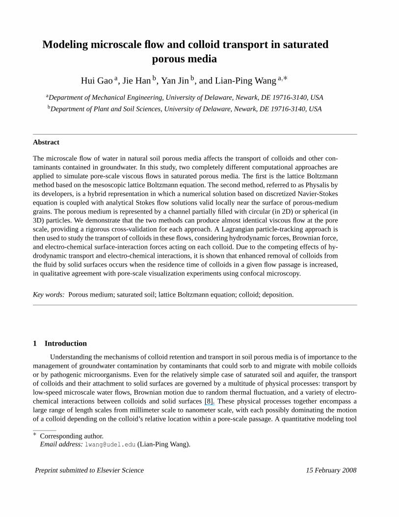
Consider a viscous flow in a two-dimensional channel with 7 fixed cylinders as shown in Fig. 1. This two-dimensional setting is used to mimic a slice of a 0.8mm×0.8mm channel packed with glass beads (0.20 mm indiameter) (i.e., see Fig. 10 below). Flow is driven by a constant pressure gradient or a body force in the y direction.Periodic boundary condition is assumed in flow direction with a periodicity length of L, while no-slip velocitycondition is applied on the two sidewalls at x = 0 and x = H, and on the surface of the 7 glass cylinders. Thechannel width H is set to 200 and the cylinders have an identical diameter of 30. The computational domain sizein terms of the grid-spacing (dx = dy = 1) is 200 in the x direction and 93 in the y direction. The centers of the 7cylinders are located at (50,25), (100,25), (150,25), (25,68), (75,68), (125,68), and (175,68), respectively.

At the initial time t = 0, the fluid is at rest. The body force per unit volume is set to FB = 8ρνUc/H2, suchthat the centerline velocity of the channel would be Uc at long time when the body force is balanced by the viscouseffects, if there were no glass cylinders in the channel. Here ν and ρ are the fluid kinematic viscosity and density,respectively. The magnitude of Uc is adjusted to match the flow rate in our microchannel flow experiment. For theresults discussed here, Uc is such that the Reynolds number based on Uc and H is UcH/ν = 0.20025.

2.1 The lattice Boltzmann approach

In the LBM approach, the lattice-Boltzmann equation for the distribution function f i of the mesoscopicparticle with velocity ei

2

Fig. 1. A sketch of the two dimensional channel with 7 fixed glass beads.

fi(x+ eiδt , t +δt)− fi(x, t) = −1τ

[

fi(x, t)− f (eq)i (x, t)

]

+ψi(x, t) (1)

is solved with a prescribed forcing field ψi designed to model the driving pressure gradient or body force. In thiswork, ψi is specified as ψi(x, t) = Wiei ·F/c2

s , where F is the macroscopic force per unit mass acting on the fluid.The standard D2Q9 lattice model in 2D and the D3Q19 model in 3D [26] are used with the following equilibriumdistribution function

f (eq)i (x, t) = Wi

[

ρ+ρ0ei ·u

c2s

+ρ0uu : (eiei − c2

s I)2c4

s

]

, (2)

where Wi is the weight, the sound speed cs is 1/√

3, and I ≡ [δi j] is the second-order identity tensor. The meandensity ρ0 is set to 1.0. The macroscopic hydrodynamic variables are computed as

ρ = ∑i

fi, ρ0u = ∑i

fiei, p = ρc2s , (3)

where ρ, u, and p are the fluid density fluctuation (the local fluid density is ρ0 + ρ), velocity, and pressure, re-spectively. The above form of the equilibrium distribution was suggested by He and Luo [13] to best model theincompressible Navier-Stokes equation.

A uniform lattice is used to cover the computational domain. The straight channel walls are located in themiddle of lattice links so a second-order accuracy is achieved with a simple bounce-back implementation. The inletand outlet are also located half way on the lattice links to facilitate the implementation of the periodic boundarycondition in the y direction.

The key implementation issue here is the treatment of solid particle surfaces. For each lattice node near aparticle surface, we identify all links moving into the surface and their relative boundary-cutting location, namely,the percentage (α) of a link located outside the surface. Since particles are fixed, this information is pre-processedbefore the flow evolution. Before the streaming step, the missing population is properly interpolated in terms of αand two populations lying before and after the path of the missing population [32,20]. For results in this paper, weused the first-order interpolation based on two known populations, and found that the results are quite similar to thesecond-order interpolation based on three nodes [20]. All lattice nodes lying within the solid particles (including

3

the fluid-solid interface) are excluded from LBE evolution, their velocities are simply set to zero. As a validationcheck, the total mass for the fluid nodes (excluding the fluid-solid interface nodes) is computed and found to remainconstant as time is advanced.

We also tested the generalized lattice Boltzmann equation or the multiple-relaxation-time (MRT) model aspresented in [19,16]. The MRT has been shown to improve numerical stability so flows at higher Reynolds numberscan be simulated. Here our flow is at low flow Reynolds number, but we will demonstrate an interesting robustnessof MRT which allows a wider range of relaxation parameter (or viscosity setting) to be used in the LBM approach,when compared to the usual BGK collision model shown in Eq. (1).

2.2 The Navier-Stokes approach: Physalis

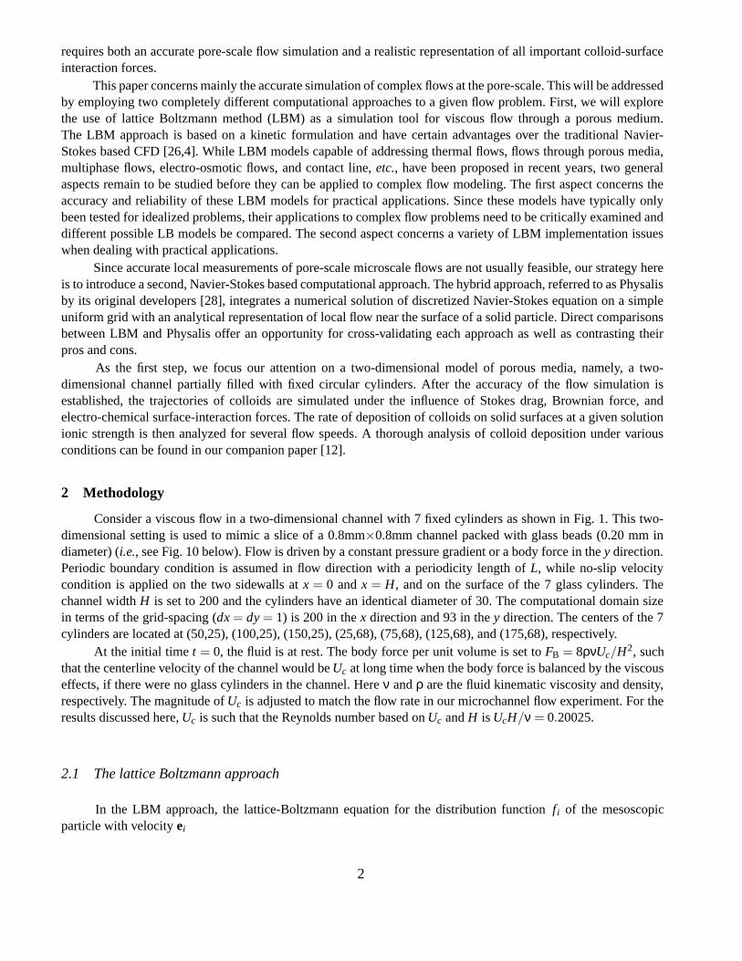
To validate the lattice Boltzmann approach and compare it with traditional Navier-Stokes based computa-tional approaches, we also developed a code using the hybrid method proposed by Prosperetti and co-workers [28,33,34].The method was named Physalis [28]. Physalis combines a numerical discrete representation of the Navier-Stokesviscous flow around particles and an analytical representation imbedded near the surface of each particle.

Fig. 2. The cage used to represent a glass bead surface in Physalis, for a glass bead with a radius of 15 grid spacings.Solid circles denote pressure cage nodes, open circles are vorticity cage nodes, filled triangles are u-velocity cagenodes, and open triangles are v-velocity cage nodes. The thick line denotes the glass bead surface.

The basic idea behind Physalis is as follows. Because of the no-slip boundary conditions on its surface, asolid particle induces a specific local flow structure that could be used to linearize the Navier-Stokes equations inthe neighborhood of the particle surface. The fluid velocity, pressure, and vorticity near the particle surface canbe expressed analytically using series solutions of Stokes flow equations. As a result, the geometric surface of theparticle can be replaced by a Stokes flow solution valid in a narrow but finite region near the surface, known as thecage region as indicated by the two dash circles in Figure 2.

4

There are three main components in Physalis. The first component is an analytical representation of the flowwithin the cage region. This is obtained by the method of separation of variables applied to Stokes flow equations.The general form in 2D is given in [33] and in 3D is found in [34,10]. The second component is the numericalmethod for Navier-Stokes equations on a regular mesh (the flow solver). The second-order project method [3] isused. The intermediate velocity in the fractional step procedure is solved by a factorization method [17], while thePoisson equation for the projection step is solved by a combination of transformation and tridiagonal inversion.This mesh extends to the interior of the particle surface. The velocity cage essentially defines an internal boundaryfor the viscous flow where the Stokes solution is employed to specify the boundary conditions there.

The most essential component is the coupling or matching between the numerical solution on the regularmesh and the Stokes solution in the cage. This coupling is achieved by an iterative procedure in which (a) thenumerical solution is used to refine the coefficients in the Stokes flow representation and in turn (b) the numericalsolution is refined by an updated boundary conditions at the velocity cage from the refined Stokes flow. The first partis accomplished by a Singular Value Decomposition algorithm since an overspecified linear system (the number ofcage nodes used for coupling is larger than the number of coefficients) is to be solved. The second part currentlyrelies only on the specific method of defining the cage velocity nodes or the internal boundary, so the analyticalnature of the Stokes solution may not be fully taken advantage of. There are more than one way to specify the cageregion [28]. For accuracy of the Stokes flow representation, it is desirable to select the cage nodes as close to thesurface of the particle as possible.

An important advantage of this hybrid method is that the force and torque acting on the particle can becalculated directly from the Stokes solution, avoiding often tedious numerical integration of local viscous force onthe particle surface that is necessary for other non-hybrid numerical methods.

2.3 Dynamics of colloids

When the steady viscous flow is established in the microscale porous channel, colloids are randomly injectedinto the flow at the inlet with a velocity equal to the local fluid velocity, at a rate that corresponds to a concentrationof 1 ppm. One ppm indicates that the colloid mass concentration is 1 mg/L or a number concentration of 1810 permm3 of the solution. If we assume that the two-dimensional flow model represents a slice of thickness equal to thecolloid radius, then the above concentration implies that there are about 23.7 colloids in the periodic fluid domainshown in Fig. 1. Since this concentration is very low, the fluid flow is assumed to be unaffected by the presenceof colloids. Each colloid is treated as a discrete entity (point-like particle) and moves according to the followingequation of motion

mcdv(t)

dt= Fdrag +Fb +Fg +FB +Fc, (4)

where v(t) is the instantaneous (Lagrangian) velocity of the colloid, mc ≡ 4πρca3c/3 is the mass of the colloid,

ρc is the material density of the colloid, and ac is the radius of the colloid. All relevant physical parameters andtheir corresponding value in the numerical simulation are shown in Table 1. The hydrodynamic forces include theviscous drag Fdrag and the buoyancy force Fb. Other forces such as the pressure-gradient force, the added mass,Basset history term [22] are neglected here due to the very slow solvent (water) flow. Fg is the gravitational bodyforce. FB is a random force designed to simulate Brownian motion of the colloid due to local thermal fluctuationsof solvent molecules. Finally, Fc represents interaction forces of the colloid with the glass (grain and wall) surfaceor other deposited colloids. The colloid is assumed to have a radius of ac = 0.5 µm, this together with the slowStokes flow of the solvent implies that a Stokes drag could be assumed, namely,

Fdrag = ζ(u(Y(t), t)−v(t)) , with ζ ≡ 6πµac, (5)

5

Table 1Physical parameters and their value in the numerical simulation.

Symbol Physical value Value in simulation

water density ρ 1000 kg/m3 1

water viscosity µ 0.001 kg/(m.s) 0.8

grid spacing dx, dy 2 µm 1

channel width H 800 µm 400

periodicity length L 372 µm 186

glass cylinder radius R 60 µm 30

colloid radius ac 0.5 µm 0.25

velocity used in setting FB Uc 679.5 m/day 0.01258

mean speed realized Us 2.887 m/day 5.347×10−5

porosity ε 0.734 0.734

nominal flow speed Us/ε ∼ 4.0 m/day 7.285×10−5

colloid density ρc 1055 kg/m3 1.055

time step dt 6.4×10−5 s 20

mass of colloid (actual) mc 5.524×10−16 kg 0.06905

mass of colloid (assumed) m∗c 6.033×10−12 kg 754.0

response time (actual) τc 5.86×10−8 s 1.831×10−2

response time (assumed) τ∗c 6.4×10−4 s 200

force Fdrag,Fc, etc. (1.563×10−9)F N F

where u(x, t) is the Eulerian solvent velocity field, Y(t) is the instantaneous location of the colloid obtained fromthe kinematic equation dY(t)/dt = v(t), and µ is the solvent viscosity. As the first step, we neglected the effects oflocal fluid shear and any corrections of the viscous force due to glass cylinder surface or channel wall. Local shearflow may induce viscous force (i.e., lift force) normal to the flow [27,23]. Hydrodynamic interaction of the colloidwith a surface can result in a modified drag, additional lift, and non-zero torque [11,25]. These modifications couldbe included in our Lagrangian colloid-tracking approach. Here we chose to keep the force formulation simplefor the following reasons: (a) in a study conducted by Arcen et al. [2], it was shown that the results of particlestatistical properties from numerical simulation based on the standard drag force only are not much differentfrom these obtained using wall-corrected drag and lift forces; (b) computations of wall and shear corrections arecomputationally expensive; (c) there appear to be inconsistencies in the literature regarding the general expressionof viscous force acting on a particle in a shear flow near a surface; and (d) we intend to develop a systematicunderstanding by gradually adding complexity to the description of hydrodynamic forces, one step at a time.

The Stokes inertial response time of the colloid τc ≡ mc/ζ = 2ρca2c/(9µ) is about 5.86× 10−8 s, which is

much smaller than the typical flow time scale. Therefore, the colloid would move along a streamline if no otherforces were considered. In the numerical simulation, we assumed a value of τ∗c = 6.4× 10−4 s, which is severalorder of magnitude larger than the actual value, but is still very much smaller than the flow time scale, in order to

6

(a) (b)

h/ac h/ac

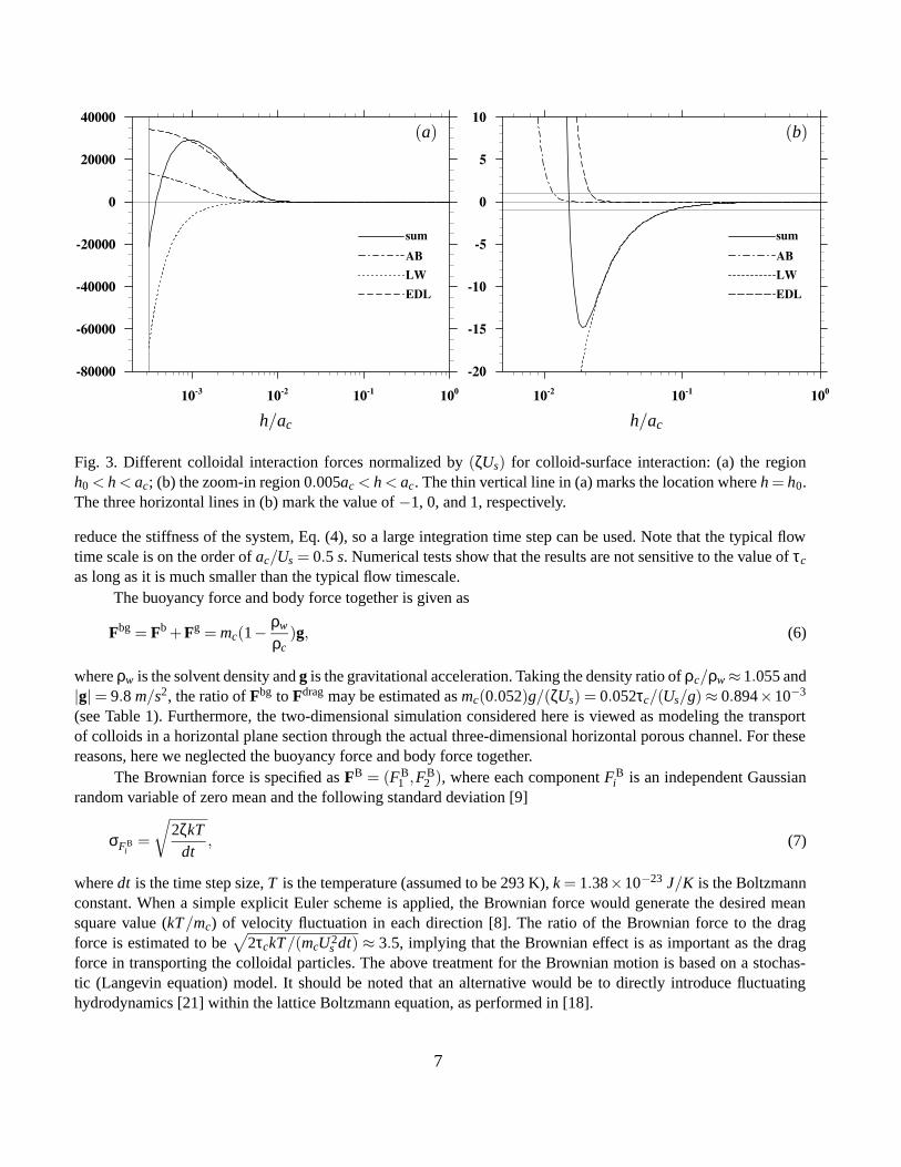
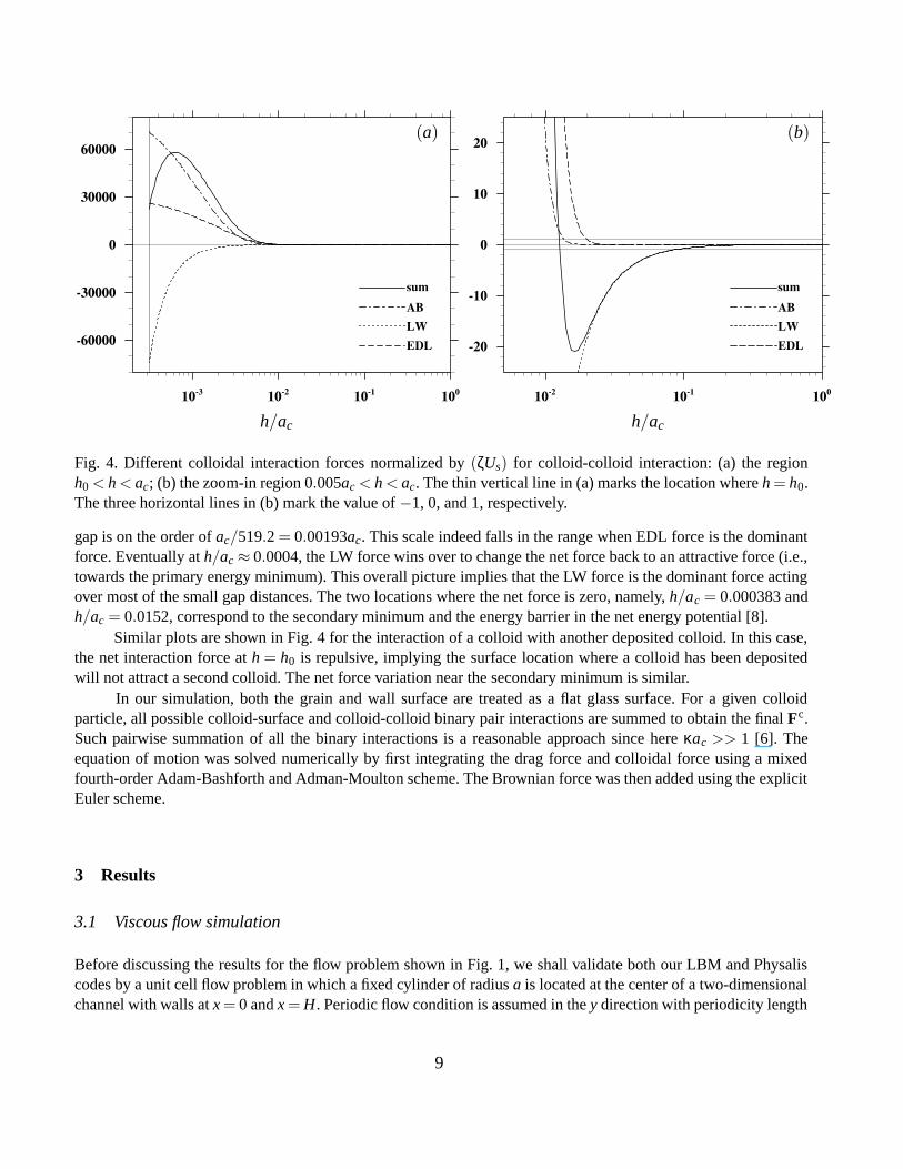
Fig. 3. Different colloidal interaction forces normalized by (ζUs) for colloid-surface interaction: (a) the regionh0 < h < ac; (b) the zoom-in region 0.005ac < h < ac. The thin vertical line in (a) marks the location where h = h0.The three horizontal lines in (b) mark the value of −1, 0, and 1, respectively.

reduce the stiffness of the system, Eq. (4), so a large integration time step can be used. Note that the typical flowtime scale is on the order of ac/Us = 0.5 s. Numerical tests show that the results are not sensitive to the value of τc

as long as it is much smaller than the typical flow timescale.The buoyancy force and body force together is given as

Fbg = Fb +Fg = mc(1−ρw

ρc)g, (6)

where ρw is the solvent density and g is the gravitational acceleration. Taking the density ratio of ρc/ρw ≈ 1.055 and|g| = 9.8 m/s2, the ratio of Fbg to Fdrag may be estimated as mc(0.052)g/(ζUs) = 0.052τc/(Us/g) ≈ 0.894×10−3

(see Table 1). Furthermore, the two-dimensional simulation considered here is viewed as modeling the transportof colloids in a horizontal plane section through the actual three-dimensional horizontal porous channel. For thesereasons, here we neglected the buoyancy force and body force together.

The Brownian force is specified as FB = (FB1 ,FB

2 ), where each component FBi is an independent Gaussian

random variable of zero mean and the following standard deviation [9]

σFBi

=

√

2ζkTdt

, (7)

where dt is the time step size, T is the temperature (assumed to be 293 K), k = 1.38×10−23 J/K is the Boltzmannconstant. When a simple explicit Euler scheme is applied, the Brownian force would generate the desired meansquare value (kT/mc) of velocity fluctuation in each direction [8]. The ratio of the Brownian force to the dragforce is estimated to be

√

2τckT/(mcU2s dt) ≈ 3.5, implying that the Brownian effect is as important as the drag

force in transporting the colloidal particles. The above treatment for the Brownian motion is based on a stochas-tic (Langevin equation) model. It should be noted that an alternative would be to directly introduce fluctuatinghydrodynamics [21] within the lattice Boltzmann equation, as performed in [18].

7

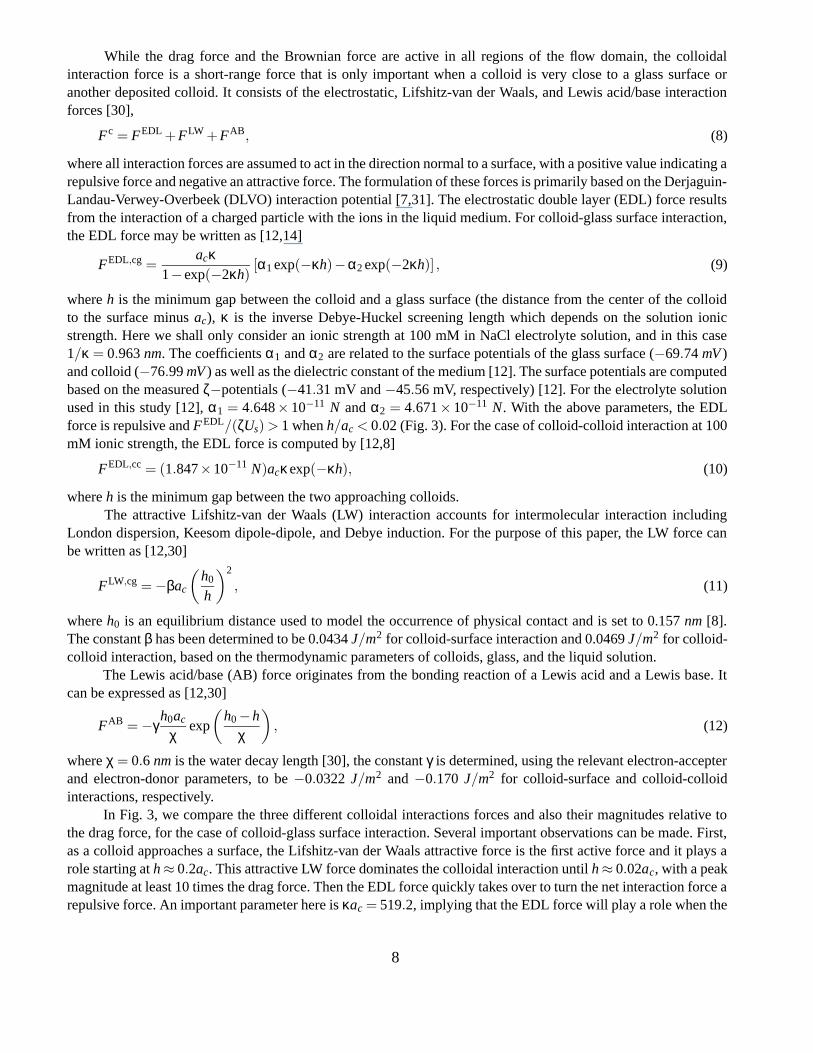
While the drag force and the Brownian force are active in all regions of the flow domain, the colloidalinteraction force is a short-range force that is only important when a colloid is very close to a glass surface oranother deposited colloid. It consists of the electrostatic, Lifshitz-van der Waals, and Lewis acid/base interactionforces [30],

Fc = FEDL +FLW +FAB, (8)

where all interaction forces are assumed to act in the direction normal to a surface, with a positive value indicating arepulsive force and negative an attractive force. The formulation of these forces is primarily based on the Derjaguin-Landau-Verwey-Overbeek (DLVO) interaction potential [7,31]. The electrostatic double layer (EDL) force resultsfrom the interaction of a charged particle with the ions in the liquid medium. For colloid-glass surface interaction,the EDL force may be written as [12,14]

FEDL,cg =acκ

1− exp(−2κh)[α1 exp(−κh)−α2 exp(−2κh)] , (9)

where h is the minimum gap between the colloid and a glass surface (the distance from the center of the colloidto the surface minus ac), κ is the inverse Debye-Huckel screening length which depends on the solution ionicstrength. Here we shall only consider an ionic strength at 100 mM in NaCl electrolyte solution, and in this case1/κ = 0.963 nm. The coefficients α1 and α2 are related to the surface potentials of the glass surface (−69.74 mV )and colloid (−76.99 mV ) as well as the dielectric constant of the medium [12]. The surface potentials are computedbased on the measured ζ−potentials (−41.31 mV and −45.56 mV, respectively) [12]. For the electrolyte solutionused in this study [12], α1 = 4.648× 10−11 N and α2 = 4.671× 10−11 N. With the above parameters, the EDLforce is repulsive and FEDL/(ζUs) > 1 when h/ac < 0.02 (Fig. 3). For the case of colloid-colloid interaction at 100mM ionic strength, the EDL force is computed by [12,8]

FEDL,cc = (1.847×10−11 N)acκexp(−κh), (10)

where h is the minimum gap between the two approaching colloids.The attractive Lifshitz-van der Waals (LW) interaction accounts for intermolecular interaction including

London dispersion, Keesom dipole-dipole, and Debye induction. For the purpose of this paper, the LW force canbe written as [12,30]

FLW,cg = −βac

(

h0

h

)2

, (11)

where h0 is an equilibrium distance used to model the occurrence of physical contact and is set to 0.157 nm [8].The constant β has been determined to be 0.0434 J/m2 for colloid-surface interaction and 0.0469 J/m2 for colloid-colloid interaction, based on the thermodynamic parameters of colloids, glass, and the liquid solution.

The Lewis acid/base (AB) force originates from the bonding reaction of a Lewis acid and a Lewis base. Itcan be expressed as [12,30]

FAB = −γh0ac

χexp

(

h0 −hχ

)

, (12)

where χ = 0.6 nm is the water decay length [30], the constant γ is determined, using the relevant electron-accepterand electron-donor parameters, to be −0.0322 J/m2 and −0.170 J/m2 for colloid-surface and colloid-colloidinteractions, respectively.

In Fig. 3, we compare the three different colloidal interactions forces and also their magnitudes relative tothe drag force, for the case of colloid-glass surface interaction. Several important observations can be made. First,as a colloid approaches a surface, the Lifshitz-van der Waals attractive force is the first active force and it plays arole starting at h ≈ 0.2ac. This attractive LW force dominates the colloidal interaction until h ≈ 0.02ac, with a peakmagnitude at least 10 times the drag force. Then the EDL force quickly takes over to turn the net interaction force arepulsive force. An important parameter here is κac = 519.2, implying that the EDL force will play a role when the

8

(a) (b)

h/ac h/ac

Fig. 4. Different colloidal interaction forces normalized by (ζUs) for colloid-colloid interaction: (a) the regionh0 < h < ac; (b) the zoom-in region 0.005ac < h < ac. The thin vertical line in (a) marks the location where h = h0.The three horizontal lines in (b) mark the value of −1, 0, and 1, respectively.

gap is on the order of ac/519.2 = 0.00193ac. This scale indeed falls in the range when EDL force is the dominantforce. Eventually at h/ac ≈ 0.0004, the LW force wins over to change the net force back to an attractive force (i.e.,towards the primary energy minimum). This overall picture implies that the LW force is the dominant force actingover most of the small gap distances. The two locations where the net force is zero, namely, h/ac = 0.000383 andh/ac = 0.0152, correspond to the secondary minimum and the energy barrier in the net energy potential [8].

Similar plots are shown in Fig. 4 for the interaction of a colloid with another deposited colloid. In this case,the net interaction force at h = h0 is repulsive, implying the surface location where a colloid has been depositedwill not attract a second colloid. The net force variation near the secondary minimum is similar.

In our simulation, both the grain and wall surface are treated as a flat glass surface. For a given colloidparticle, all possible colloid-surface and colloid-colloid binary pair interactions are summed to obtain the final Fc.Such pairwise summation of all the binary interactions is a reasonable approach since here κac >> 1 [6]. Theequation of motion was solved numerically by first integrating the drag force and colloidal force using a mixedfourth-order Adam-Bashforth and Adman-Moulton scheme. The Brownian force was then added using the explicitEuler scheme.

3 Results

3.1 Viscous flow simulation

Before discussing the results for the flow problem shown in Fig. 1, we shall validate both our LBM and Physaliscodes by a unit cell flow problem in which a fixed cylinder of radius a is located at the center of a two-dimensionalchannel with walls at x = 0 and x = H. Periodic flow condition is assumed in the y direction with periodicity length

9

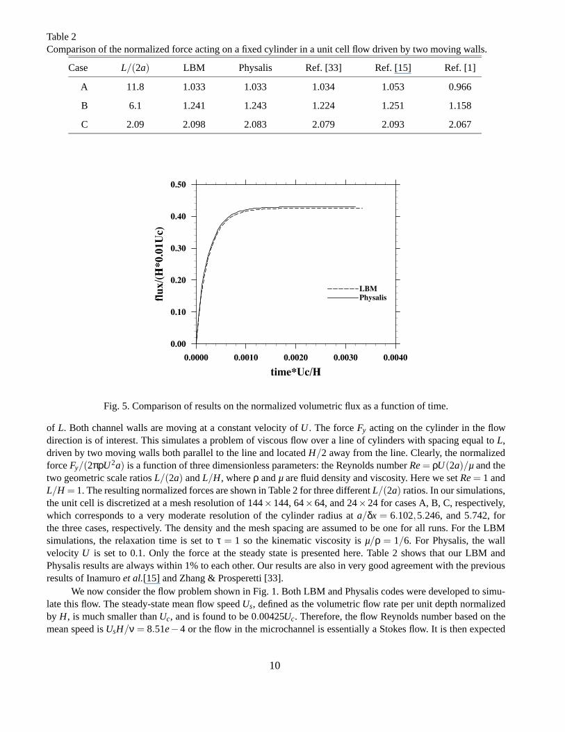
Table 2Comparison of the normalized force acting on a fixed cylinder in a unit cell flow driven by two moving walls.

Case L/(2a) LBM Physalis Ref. [33] Ref. [15] Ref. [1]

A 11.8 1.033 1.033 1.034 1.053 0.966

B 6.1 1.241 1.243 1.224 1.251 1.158

C 2.09 2.098 2.083 2.079 2.093 2.067

Fig. 5. Comparison of results on the normalized volumetric flux as a function of time.

of L. Both channel walls are moving at a constant velocity of U . The force Fy acting on the cylinder in the flowdirection is of interest. This simulates a problem of viscous flow over a line of cylinders with spacing equal to L,driven by two moving walls both parallel to the line and located H/2 away from the line. Clearly, the normalizedforce Fy/(2πρU2a) is a function of three dimensionless parameters: the Reynolds number Re = ρU(2a)/µ and thetwo geometric scale ratios L/(2a) and L/H, where ρ and µ are fluid density and viscosity. Here we set Re = 1 andL/H = 1. The resulting normalized forces are shown in Table 2 for three different L/(2a) ratios. In our simulations,the unit cell is discretized at a mesh resolution of 144×144, 64×64, and 24×24 for cases A, B, C, respectively,which corresponds to a very moderate resolution of the cylinder radius at a/δx = 6.102,5.246, and 5.742, forthe three cases, respectively. The density and the mesh spacing are assumed to be one for all runs. For the LBMsimulations, the relaxation time is set to τ = 1 so the kinematic viscosity is µ/ρ = 1/6. For Physalis, the wallvelocity U is set to 0.1. Only the force at the steady state is presented here. Table 2 shows that our LBM andPhysalis results are always within 1% to each other. Our results are also in very good agreement with the previousresults of Inamuro et al.[15] and Zhang & Prosperetti [33].

We now consider the flow problem shown in Fig. 1. Both LBM and Physalis codes were developed to simu-late this flow. The steady-state mean flow speed Us, defined as the volumetric flow rate per unit depth normalizedby H, is much smaller than Uc, and is found to be 0.00425Uc. Therefore, the flow Reynolds number based on themean speed is UsH/ν = 8.51e−4 or the flow in the microchannel is essentially a Stokes flow. It is then expected

10

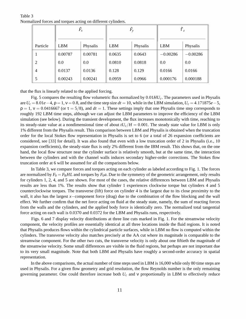
Table 3Normalized forces and torques acting on different cylinders.

F̃x F̃y Γ̃z

Particle LBM Physalis LBM Physalis LBM Physalis

1 0.00787 0.00781 0.0635 0.0643 −0.00286 −0.00286

2 0.0 0.0 0.0810 0.0818 0.0 0.0

4 0.0137 0.0136 0.128 0.129 0.0166 0.0166

5 0.00243 0.00241 0.0959 0.0966 0.000176 0.000188

that the flux is linearly related to the applied forcing.Fig. 5 compares the resulting flow volumetric flux normalized by 0.01HUc. The parameters used in Physalis

are Uc = 8.01e−4, ρ = 1, ν = 0.8, and the time step size dt = 10, while in the LBM simulation, Uc = 4.171875e−5,ρ = 1, ν = 0.0416667 (or τ = 5/8), and dt = 1. These settings imply that one Physalis time step corresponds toroughly 192 LBM time steps, although we can adjust the LBM parameters to improve the efficiency of the LBMsimulation (see below). During the transient development, the flux increases monotonically with time, reaching toits steady-state value at a nondimensional time of about tUc/H = 0.001. The steady state value for LBM is only1% different from the Physalis result. This comparison between LBM and Physalis is obtained when the truncationorder for the local Stokes flow representation in Physalis is set to 6 (or a total of 26 expansion coefficients areconsidered, see [33] for detail). It was also found that even with a low truncation order of 2 in Physalis (i.e., 10expansion coefficients), the steady-state flux is only 2% different from the IBM result. This shows that, on the onehand, the local flow structure near the cylinder surface is relatively smooth, but at the same time, the interactionbetween the cylinders and with the channel walls induces secondary higher-order corrections. The Stokes flowtruncation order at 6 will be assumed for all the comparisons below.

In Table 3, we compare forces and torques acting on each cylinder as labeled according to Fig. 1. The forcesare normalized by F0 = FBHL and torques by F0a. Due to the symmetry of the geometric arrangement, only resultsfor cylinders 1, 2, 4, and 5 are shown. For most of the cases, the relative differences between LBM and Physalisresults are less than 1%. The results show that cylinder 1 experiences clockwise torque but cylinders 4 and 5counterclockwise torques. The transverse (lift) force on cylinder 4 is the largest due to its close proximity to thewall, it also has the largest x−component force (drag) due to the combination of the flow blocking and the walleffect. We further confirm that the net force acting on fluid at the steady state, namely, the sum of reacting forcesfrom the walls and the cylinders, and the applied body force is identically zero. The normalized total tangentialforce acting on each wall is 0.0370 and 0.0372 for the LBM and Physalis runs, respectively.

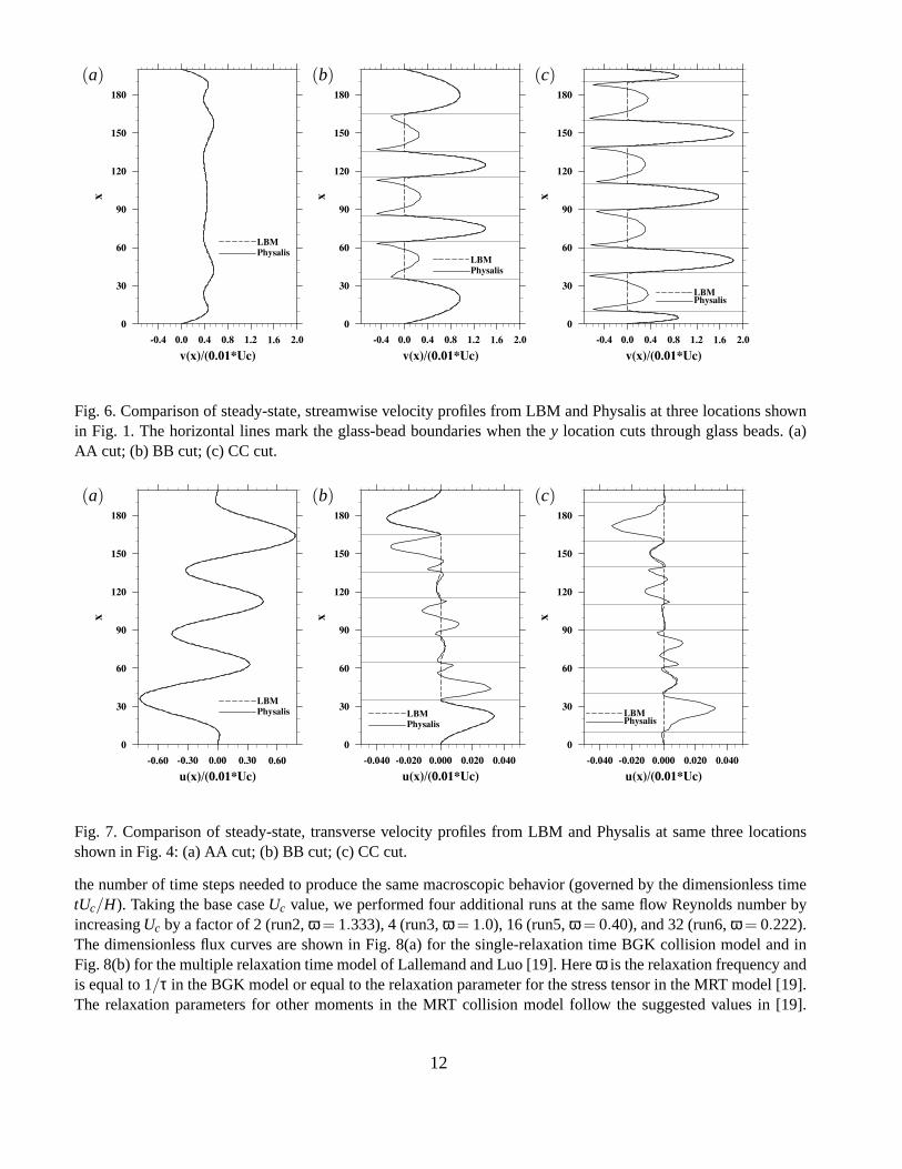
Figs. 6 and 7 display velocity distributions at three line cuts marked in Fig. 1. For the streamwise velocitycomponent, the velocity profiles are essentially identical at all three locations inside the fluid regions. It is notedthat Physalis produces flows within the cylindrical particle surfaces, while in LBM no flow is computed within thecylinders. The transverse velocity also matches precisely at the AA cut where its magnitude is comparable to thestreamwise component. For the other two cuts, the transverse velocity is only about one fiftieth the magnitude ofthe streamwise velocity. Some small differences are visible in the fluid regions, but perhaps are not important dueto its very small magnitude. Note that both LBM and Physalis have roughly a second-order accuracy in spatialrepresentation.

In the above comparisons, the actual number of time steps used in LBM is 16,000 while only 80 time steps areused in Physalis. For a given flow geometry and grid resolution, the flow Reynolds number is the only remaininggoverning parameter. One could therefore increase both Uc and ν proportionally in LBM to effectively reduce

11

(a) (b) (c)

Fig. 6. Comparison of steady-state, streamwise velocity profiles from LBM and Physalis at three locations shownin Fig. 1. The horizontal lines mark the glass-bead boundaries when the y location cuts through glass beads. (a)AA cut; (b) BB cut; (c) CC cut.

(a) (b) (c)

Fig. 7. Comparison of steady-state, transverse velocity profiles from LBM and Physalis at same three locationsshown in Fig. 4: (a) AA cut; (b) BB cut; (c) CC cut.

the number of time steps needed to produce the same macroscopic behavior (governed by the dimensionless timetUc/H). Taking the base case Uc value, we performed four additional runs at the same flow Reynolds number byincreasing Uc by a factor of 2 (run2, ω = 1.333), 4 (run3, ω = 1.0), 16 (run5, ω = 0.40), and 32 (run6, ω = 0.222).The dimensionless flux curves are shown in Fig. 8(a) for the single-relaxation time BGK collision model and inFig. 8(b) for the multiple relaxation time model of Lallemand and Luo [19]. Here ω is the relaxation frequency andis equal to 1/τ in the BGK model or equal to the relaxation parameter for the stress tensor in the MRT model [19].The relaxation parameters for other moments in the MRT collision model follow the suggested values in [19].

12

(a) (b)

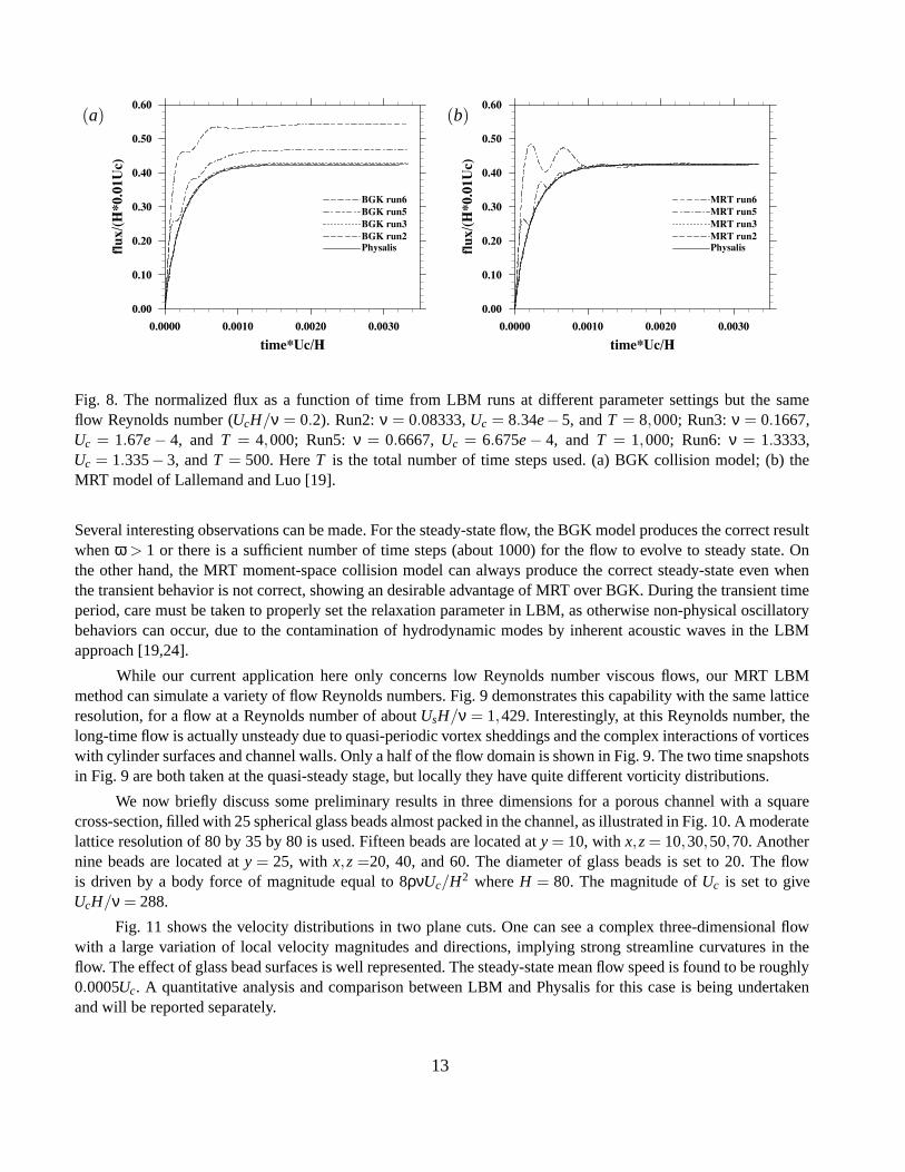
Fig. 8. The normalized flux as a function of time from LBM runs at different parameter settings but the sameflow Reynolds number (UcH/ν = 0.2). Run2: ν = 0.08333, Uc = 8.34e− 5, and T = 8,000; Run3: ν = 0.1667,Uc = 1.67e − 4, and T = 4,000; Run5: ν = 0.6667, Uc = 6.675e − 4, and T = 1,000; Run6: ν = 1.3333,Uc = 1.335− 3, and T = 500. Here T is the total number of time steps used. (a) BGK collision model; (b) theMRT model of Lallemand and Luo [19].

Several interesting observations can be made. For the steady-state flow, the BGK model produces the correct resultwhen ω > 1 or there is a sufficient number of time steps (about 1000) for the flow to evolve to steady state. Onthe other hand, the MRT moment-space collision model can always produce the correct steady-state even whenthe transient behavior is not correct, showing an desirable advantage of MRT over BGK. During the transient timeperiod, care must be taken to properly set the relaxation parameter in LBM, as otherwise non-physical oscillatorybehaviors can occur, due to the contamination of hydrodynamic modes by inherent acoustic waves in the LBMapproach [19,24].

While our current application here only concerns low Reynolds number viscous flows, our MRT LBMmethod can simulate a variety of flow Reynolds numbers. Fig. 9 demonstrates this capability with the same latticeresolution, for a flow at a Reynolds number of about UsH/ν = 1,429. Interestingly, at this Reynolds number, thelong-time flow is actually unsteady due to quasi-periodic vortex sheddings and the complex interactions of vorticeswith cylinder surfaces and channel walls. Only a half of the flow domain is shown in Fig. 9. The two time snapshotsin Fig. 9 are both taken at the quasi-steady stage, but locally they have quite different vorticity distributions.

We now briefly discuss some preliminary results in three dimensions for a porous channel with a squarecross-section, filled with 25 spherical glass beads almost packed in the channel, as illustrated in Fig. 10. A moderatelattice resolution of 80 by 35 by 80 is used. Fifteen beads are located at y = 10, with x,z = 10,30,50,70. Anothernine beads are located at y = 25, with x,z =20, 40, and 60. The diameter of glass beads is set to 20. The flowis driven by a body force of magnitude equal to 8ρνUc/H2 where H = 80. The magnitude of Uc is set to giveUcH/ν = 288.

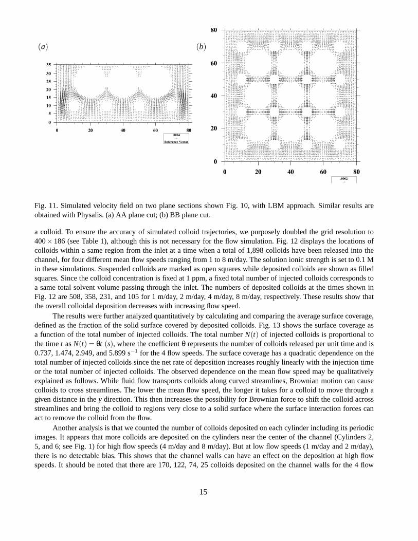
Fig. 11 shows the velocity distributions in two plane cuts. One can see a complex three-dimensional flowwith a large variation of local velocity magnitudes and directions, implying strong streamline curvatures in theflow. The effect of glass bead surfaces is well represented. The steady-state mean flow speed is found to be roughly0.0005Uc. A quantitative analysis and comparison between LBM and Physalis for this case is being undertakenand will be reported separately.

13

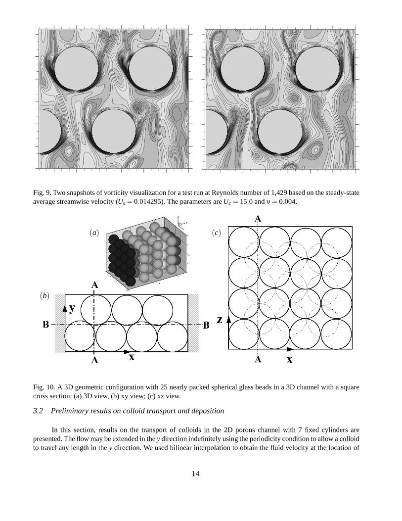
Fig. 9. Two snapshots of vorticity visualization for a test run at Reynolds number of 1,429 based on the steady-stateaverage streamwise velocity (Us = 0.014295). The parameters are Uc = 15.0 and ν = 0.004.

(a)

(b)

(c)

Fig. 10. A 3D geometric configuration with 25 nearly packed spherical glass beads in a 3D channel with a squarecross section: (a) 3D view, (b) xy view; (c) xz view.

3.2 Preliminary results on colloid transport and deposition

In this section, results on the transport of colloids in the 2D porous channel with 7 fixed cylinders arepresented. The flow may be extended in the y direction indefinitely using the periodicity condition to allow a colloidto travel any length in the y direction. We used bilinear interpolation to obtain the fluid velocity at the location of

14

(a) (b)

Fig. 11. Simulated velocity field on two plane sections shown Fig. 10, with LBM approach. Similar results areobtained with Physalis. (a) AA plane cut; (b) BB plane cut.

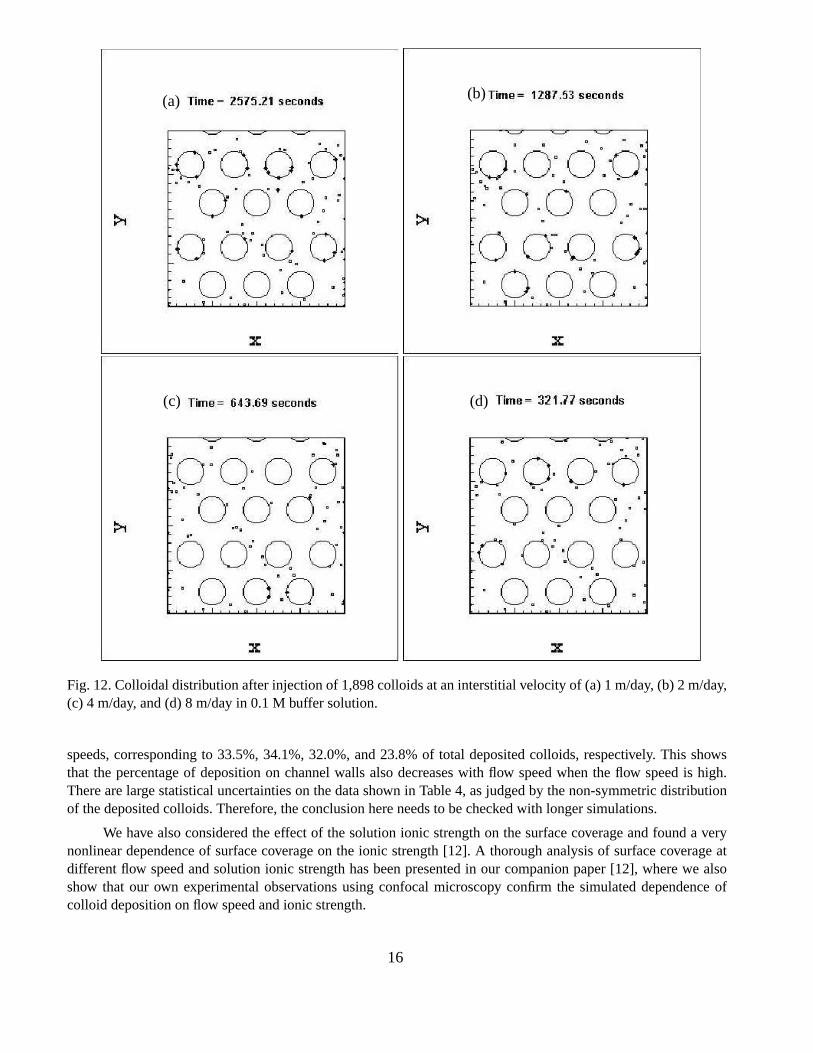
a colloid. To ensure the accuracy of simulated colloid trajectories, we purposely doubled the grid resolution to400× 186 (see Table 1), although this is not necessary for the flow simulation. Fig. 12 displays the locations ofcolloids within a same region from the inlet at a time when a total of 1,898 colloids have been released into thechannel, for four different mean flow speeds ranging from 1 to 8 m/day. The solution ionic strength is set to 0.1 Min these simulations. Suspended colloids are marked as open squares while deposited colloids are shown as filledsquares. Since the colloid concentration is fixed at 1 ppm, a fixed total number of injected colloids corresponds toa same total solvent volume passing through the inlet. The numbers of deposited colloids at the times shown inFig. 12 are 508, 358, 231, and 105 for 1 m/day, 2 m/day, 4 m/day, 8 m/day, respectively. These results show thatthe overall colloidal deposition decreases with increasing flow speed.

The results were further analyzed quantitatively by calculating and comparing the average surface coverage,defined as the fraction of the solid surface covered by deposited colloids. Fig. 13 shows the surface coverage asa function of the total number of injected colloids. The total number N(t) of injected colloids is proportional tothe time t as N(t) = θt (s), where the coefficient θ represents the number of colloids released per unit time and is0.737, 1.474, 2.949, and 5.899 s−1 for the 4 flow speeds. The surface coverage has a quadratic dependence on thetotal number of injected colloids since the net rate of deposition increases roughly linearly with the injection timeor the total number of injected colloids. The observed dependence on the mean flow speed may be qualitativelyexplained as follows. While fluid flow transports colloids along curved streamlines, Brownian motion can causecolloids to cross streamlines. The lower the mean flow speed, the longer it takes for a colloid to move through agiven distance in the y direction. This then increases the possibility for Brownian force to shift the colloid acrossstreamlines and bring the colloid to regions very close to a solid surface where the surface interaction forces canact to remove the colloid from the flow.

Another analysis is that we counted the number of colloids deposited on each cylinder including its periodicimages. It appears that more colloids are deposited on the cylinders near the center of the channel (Cylinders 2,5, and 6; see Fig. 1) for high flow speeds (4 m/day and 8 m/day). But at low flow speeds (1 m/day and 2 m/day),there is no detectable bias. This shows that the channel walls can have an effect on the deposition at high flowspeeds. It should be noted that there are 170, 122, 74, 25 colloids deposited on the channel walls for the 4 flow

15

(a) (b)

(c) (d)

Fig. 12. Colloidal distribution after injection of 1,898 colloids at an interstitial velocity of (a) 1 m/day, (b) 2 m/day,(c) 4 m/day, and (d) 8 m/day in 0.1 M buffer solution.

speeds, corresponding to 33.5%, 34.1%, 32.0%, and 23.8% of total deposited colloids, respectively. This showsthat the percentage of deposition on channel walls also decreases with flow speed when the flow speed is high.There are large statistical uncertainties on the data shown in Table 4, as judged by the non-symmetric distributionof the deposited colloids. Therefore, the conclusion here needs to be checked with longer simulations.

We have also considered the effect of the solution ionic strength on the surface coverage and found a verynonlinear dependence of surface coverage on the ionic strength [12]. A thorough analysis of surface coverage atdifferent flow speed and solution ionic strength has been presented in our companion paper [12], where we alsoshow that our own experimental observations using confocal microscopy confirm the simulated dependence ofcolloid deposition on flow speed and ionic strength.

16

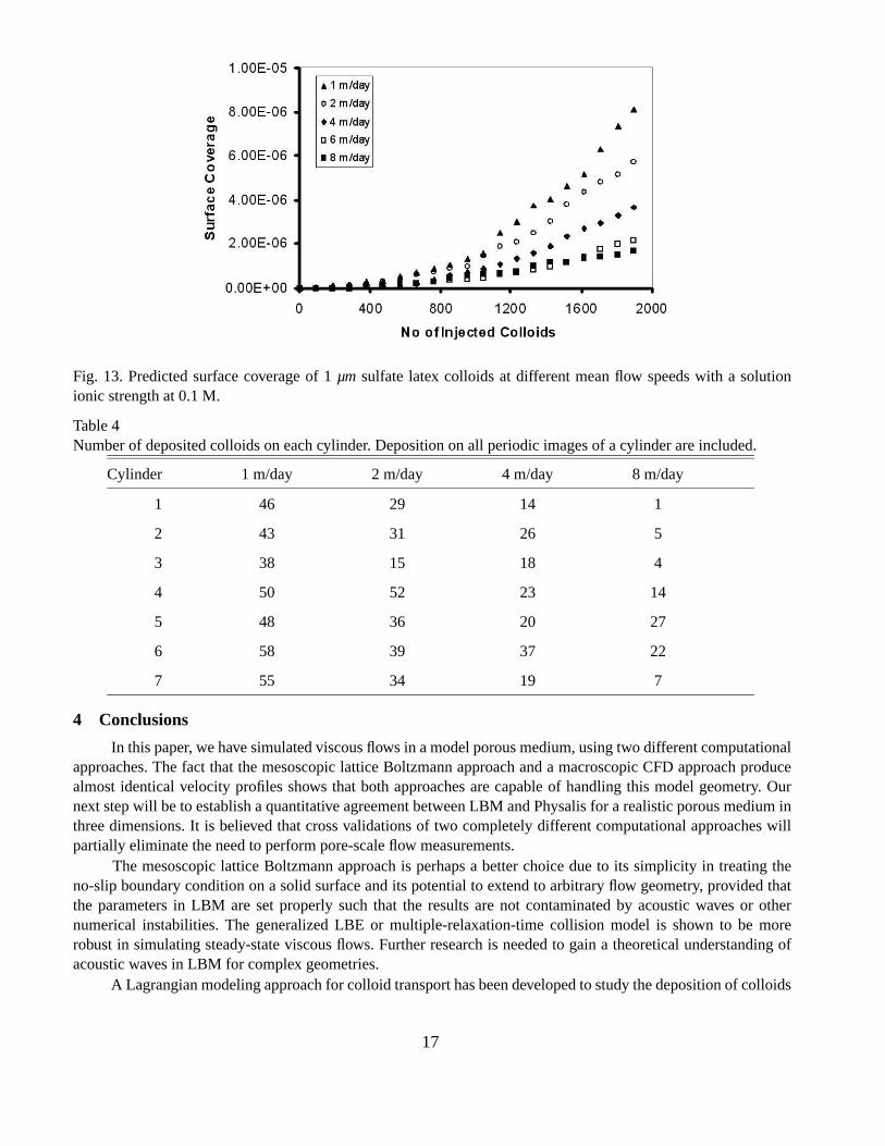
Fig. 13. Predicted surface coverage of 1 µm sulfate latex colloids at different mean flow speeds with a solutionionic strength at 0.1 M.

Table 4Number of deposited colloids on each cylinder. Deposition on all periodic images of a cylinder are included.

Cylinder 1 m/day 2 m/day 4 m/day 8 m/day

1 46 29 14 1

2 43 31 26 5

3 38 15 18 4

4 50 52 23 14

5 48 36 20 27

6 58 39 37 22

7 55 34 19 7

4 Conclusions

In this paper, we have simulated viscous flows in a model porous medium, using two different computationalapproaches. The fact that the mesoscopic lattice Boltzmann approach and a macroscopic CFD approach producealmost identical velocity profiles shows that both approaches are capable of handling this model geometry. Ournext step will be to establish a quantitative agreement between LBM and Physalis for a realistic porous medium inthree dimensions. It is believed that cross validations of two completely different computational approaches willpartially eliminate the need to perform pore-scale flow measurements.

The mesoscopic lattice Boltzmann approach is perhaps a better choice due to its simplicity in treating theno-slip boundary condition on a solid surface and its potential to extend to arbitrary flow geometry, provided thatthe parameters in LBM are set properly such that the results are not contaminated by acoustic waves or othernumerical instabilities. The generalized LBE or multiple-relaxation-time collision model is shown to be morerobust in simulating steady-state viscous flows. Further research is needed to gain a theoretical understanding ofacoustic waves in LBM for complex geometries.

A Lagrangian modeling approach for colloid transport has been developed to study the deposition of colloids

17

on solid surface. The key finding is that the rate of deposition depends on the flow speed and solution ionic strength,and the nature of the dependence agrees qualitatively with previous observations and our visualizations usingconfocal microscopy [12]. This demonstrates the feasibility of our computational model as a quantitative researchtool and its potential for revealing transport mechanisms at the pore scale. We intend to develop this model furtherto include other hydrodynamic interaction forces and three-dimensional flow effects, so a quantitative comparisonwith pore-scale experimental observations can be made possible. It is important to note that, because typicallyκac >> 1, the hydrodynamic interaction forces become active far before the electrostatic double layer interactionforce.

Acknowledgements. This study is supported by the U.S. Department of Agriculture (NRI, 2006-02551), U.S.National Science Foundation (ATM-0527140), and National Natural Science Foundation of China (Project No.10628206). The authors thank Ms. V.I. Lazouskaya for helpful discussions on the general topic of colloidal trans-port in both saturated and unsaturated soil.

References

[1] C.K. Aidun and Y. Lu 1995 Lattice Boltzmann simulation of solid particles suspended in a fluid. J. Stat. Phys.81: 49-61.

[2] O. Arcen, A. Taniere, and B. Oesterle, Int. J. Multiphase Flow 32 (2006) 1326-1339.

[3] D.L. Brown, R. Cortez, and M.L. Minion, J. Comp. Phys. 168 (2001) 464-499.

[4] S. Chen and G. Doolen, Annu. Rev. Fluid Mech. 30 (1998) 329-364.

[5] Y. Chu, Y. Jin, M. V. Yates, J. Environ. Qual., 29 (2000) 1103-1110.

[6] P.K. Das and S. Bhattacharjee 2005, Electrostatic double layer force between a sphere and a planar substratein the presence of previously deposited spherical particles. Langmuir, 21: 4755-4764.

[7] B.V. Derjaguin and L. Landau, 1941. Theory of the stability of strongly charged lyophobic sols and of theadhesion of strongly charged particles in solutions of electrolytes. Acta Physicochem (USSR) 1941, 14, 633-662.

[8] M.J. Elimelech, J. Gregory, X. Jia, and R. A. Williams, 1995, Particle Deposition and Aggregation:Measurement, Modeling, and Simulation, Butterworth-Heinemann, Oxford.

[9] M. Fujita, H. Nishikawa, T. Okubo, and Y. Yamaguchi. J. Appl. Phys. 42 (2004) 4434-4442

[10] H. Gao and L.-P. Wang, Paper 713, CDROM Proceedings of the 6th International Conference on MultiphaseFlow, Leipzig, Germany, July 9–17, 2007.

[11] A.J., Goldman, A.J., Cox R.G., and H. Brenner, Chem. Eng. Sci. 22 (1967) 653 - 660.

[12] J. Han, H. Gao, L.-P. Wang, and Y. Jin, 2008 Pore-scale investigations of flow speed and ionic strength oncolloid deposition in saturated media. Submitted to Langmuir..

[13] X. He, L.-S. Luo, I. Stat. Phys. 88 (1997) 927-944.

[14] Hogg, R., T. W. Healy, D. W. T. Fuerstenau. 1966. Mutual coagulation of colloidal dispersions. Faraday Soc.,62, 1638-1651.

[15] T. Inamuro, K.Maeba, and F. Ogino 2000, Flow between parallel walls containing a line of neutrally buoyantcircular cylinders. Int. J. Multiphase Flow, 26, 1981-2004.

[16] D. d’Humieres, I. Ginzburg, K. Krafczyk, P. Lallemand and L.-S. Luo, Phil. Trans. Roy. Soc. London A. 360(2002): 437-451.

[17] Kim, J. and P. Moin, J. Comp. Phys. 59 (1985) 308-323.

[18] A.J.C. Ladd 1993 Short-time motion of colloidal particles: Numerical simulation via a fluctuating lattice-Boltzmann equation. Phys. Rev. Lett. 70: 1339-1342.

18

[19] P. Lallemand and L.-S. Luo, Physical Review E. 61 (2000), 6546-6562.

[20] P. Lallemand and L.-S. Luo, J. Comp. Phys. 184 (2003), 406-421.

[21] L. Landau and E. Lifshitz, 1959, Fluid Mechanics, Addison-Wesley, London.

[22] M.R. Maxey and J.J. Riley, Phys. Fluids 26 (1983) 883 - 889.

[23] J.B., McLaughlin, J. Fluid Mech. 224 (1991) 261-274.

[24] R. Mei, L.-L. Luo, P. Lallemand, D. d’Humieres, Computers & Fluids 35 (2006) 855-862.

[25] M.E., O’Neill, Chem. Eng. Sci. 23 (1968) 1293 - 1298.

[26] Y. Qian, S. Succi, and S.A. Orszag, Annu. Rev. Comput. Phys. 3 (1995) 195-242.

[27] P.G., Saffman, J. Fluid Mech. 22 (1965) 385-340.

[28] S. Takagi, H.N. Oguz, Z. Zhang, A. Prosperetti, J. Comp. Phys. 187 (2003) 371-390.

[29] S.S. Thompson and M. V. Yates, Appl. Environ. Microbiol, 65 (1999) 1186-1190.

[30] van Oss, C. J. 1994. Interfacial forces in aqueous media. Marcel Dekker, New York.

[31] E.J. Verwey and J.T.G. Overbeek, 1948 Theory of Stability of Lyophobic Colloids, Elsevier, Amsterdam.

[32] D. Yu, R. Mei, L.-S. Luo, and W. Shyy, Progress in Aerospace Sci. 39 (2003) 329-367.

[33] Z. Zhang, A. Prosperetti, J. Appl. Mech. Trans. ASME 70 (2003) 64-74

[34] Z. Zhang, A. Prosperetti, J. Comp. Phys. 210 (2005) 292-324.

19