MODELLING FOR ENGINEERING AND HUMAN BEHAVIOUR 2015 Instituto Universitario de Matemática Multidisciplinar L. Jódar, L. Acedo and J. C. Cortés ( Editors ) Instituto Universitario de Matemática Multidisciplinar

Welcome message from author
This document is posted to help you gain knowledge. Please leave a comment to let me know what you think about it! Share it to your friends and learn new things together.
Transcript

MODELLING FOR ENGINEERING AND HUMAN BEHAVIOUR
2015Instituto Universitario de Matemática Multidisciplinar
L. Jódar, L. Acedo and J. C. Cortés ( Editors )
Instituto Universitario de Matemática Multidisciplinar

MODELLING FOR ENGINEERING,
& HUMAN BEHAVIOUR 2015
Instituto Universitario de Matematica Multidisciplinar
Universitat Politecnica de Valencia
Valencia 46022, SPAIN
Edited byLucas Jodar, Luis Acedo and Juan Carlos CortesInstituto Universitario de Matematica MultidisciplinarUniversitat Politecnica de ValenciaI.S.B.N.: 978-84-608-5355-8

CONTENTS
1. Modelling the flyby anomaly in a Whiteheadian theory of gravity, by L. AcedoPag: 1-5
2. Supply schedule in intermittent water supply based on quantitative and qualita-tive criteria, by A. E. Ilaya-Ayza, R. Perez-Garcıa, J. Izquierdo and J. Benıtez . . . . . .Pag:6-11
3. Internal Lubricant Content in inhalation Capsules, by G. Ayala, F. Dıez, M. T. Gassoand B. E. Jones . . . . . . . . . . . . . . . . . . . . . . . . . . . . . . . . . . . . . . . . . . . . . . . . . . . . . . . . . . . . . . . .Pag: 12-15
4. Microscopic and macroscopic models for gas leak detection, by F. Aznar, M. Pujoland R. Rizo . . . . . . . . . . . . . . . . . . . . . . . . . . . . . . . . . . . . . . . . . . . . . . . . . . . . . . . . . . . . . . . . . . . Pag: 16-20
5. Modelling the survival of the Spanish construction SME in a crisis environment,by I. Barrachina and E. de la Poza . . . . . . . . . . . . . . . . . . . . . . . . . . . . . . . . . . . . . . . . . . . . .Pag: 21-25
6. An algorithm for quasi-linear control problems in the economics of renewableresources: The steady state and end state for the infinite and long-term horizon,by L. Bayon, P. J. Garcıa-Nieto, R. Garcıa-Rubio, J. A. Otero and C. Tasis . . . . Pag: 26-31
7. A polynomial expansion method based on Helmholtz equation for the NeutronDiffusion Equation discretized by the Finite Volume Method, by A. Bernal, J. E.Roman, R. Miro and G. Verdu . . . . . . . . . . . . . . . . . . . . . . . . . . . . . . . . . . . . . . . . . . . . . . . . . Pag: 32-37
8. On the matrix Hill’s equation and its applications to engineering models, by P.Bader, S. Blanes, E. Ponsoda and M. Seydaoglu . . . . . . . . . . . . . . . . . . . . . . . . . . . . . . . Pag: 38-43
9. Adaptability of the acoustics of a room by varying the height of the acousticceiling, by P. J. Blazquez and L. Orcos . . . . . . . . . . . . . . . . . . . . . . . . . . . . . . . . . . . . . . . .Pag: 44-49
10. Water pump scheduling Optimization using Agent Swarm Optimization, by B.Brentan, I. Montalvo, E. Luvizotto Jr., J. Izquierdo and R. Perez-Garcıa . . . . . . . Pag: 50-55
11. Mathematical modelling of health care expenditure adjusted by morbidity, by V.Caballer, N. Guadalajara, D. Vivas and A. Clemente . . . . . . . . . . . . . . . . . . . . . . . . . . .Pag: 56-64
12. Calculated forecast for technical obsolescence in computerised tomography equip-ment, by F. Reyes-Santıas, V. Caballer, F. Gomez, J. Rivero de Aguilar and D. Vivas Pag:65-70
13. Heuristic Framework to Jointly Calibrate Leakage and Pressure in Water Distri-bution Systems, by E. Campbell, B. Brentan, J. Izquierdo and R. Perez-Garcıa . . . . Pag:71-76
14. A novel framework to sectorize water supply networks considering uncertainties,by E. Campbell, J. Izquierdo, R. Perez-Garcıa and I. Montalvo . . . . . . . . . . . . . . . . .Pag: 77-82

15. Analysis of a class of discrete SIR epidemic model, by B. Canto, C. Coll and E.Sanchez . . . . . . . . . . . . . . . . . . . . . . . . . . . . . . . . . . . . . . . . . . . . . . . . . . . . . . . . . . . . . . . . . . . . . . . Pag: 83-86
16. Modeling Plant Virus Propagation with Delays, by M. Jackson and B. M. Chen-Charpentier . . . . . . . . . . . . . . . . . . . . . . . . . . . . . . . . . . . . . . . . . . . . . . . . . . . . . . . . . . . . . . . . . . . . . . . . . . Pag:87-92
17. A Resource-constrained scheduling problem to optimize the use of resources in adistribution center with genetic algorithms, by D. Cipres, L. Polo and P. Artaso Pag:93-98
18. Dynamical tools for better understanding the stability of high-order methods forsolving nonlinear problems, by A. Cordero, A. A. Magrenan and J. R. Torregrosa Pag:99-104
19. New Taylor algorithm for the matrix cosine, by J. Ibanez, J. Sastre, P. Alonso, J.Peinado and E. Defez . . . . . . . . . . . . . . . . . . . . . . . . . . . . . . . . . . . . . . . . . . . . . . . . . . . . . . . .Pag: 105-110
20. Modelling the spread of gender violence in Spain, by S. Barreda, E. de la Poza andL. Jodar . . . . . . . . . . . . . . . . . . . . . . . . . . . . . . . . . . . . . . . . . . . . . . . . . . . . . . . . . . . . . . . . . . . . .Pag: 111-116
21. Mathematical modelling of radicalization processes based on the example ofright-wing extremism in Germany, by T. Deutsch and M. Ehrhardt . . . . .Pag: 117-122
22. Applying the Structural Equation Model to Co-creation in Degree Programs inEcuadorian Universities, by G. Ribes, O. Pantoja and A. Peralt . . . . . . . . . . Pag: 123-128
23. Front-fixing Transformation for Regime Switching Model of American Options,by V. N. Egorova, R. Company and L. Jodar . . . . . . . . . . . . . . . . . . . . . . . . . . . . . . . . Pag: 129-134
24. Positive numerical solution of two asset jump-diffusion partial-integro differentialmodels, by M. Fakharany, R. Company and L. Jodar . . . . . . . . . . . . . . . . . . . . . . . Pag: 135-140
25. Factors Affecting the Choice Modal of Transportation in an Urban Environment.Hierarchical Multi-Criteria Analysis, by A. Fraile, J. A. Sicilia, E. Larrode and B. RoyoPag: 141-147
26. Managing dependence in Flowgraphs models. An application to Reliability En-gineering, by C. Santamarıa, B. Garcıa-Mora, G. Rubio and R. Perez-Ocon . . . . . . . . . Pag:148-153
27. Hybrid wavelet support vector machine and artificial bee colony for predictingthe cyanotoxin content from experimental cyanobacteria concentrations in theTrasona reservoir: A case study in Northern Spain, by P. J. Garcıa Nieto, E. Garcıa-Gonzalo, J. R. Alonso and C. Dıaz . . . . . . . . . . . . . . . . . . . . . . . . . . . . . . . . . . . . . . . . . . . . . . . . . . . Pag:154-160
28. Valuation of commodity derivatives under jump-diffusion processes, by L. Gomez-Valle, Z. Habibilashkary and J. Martınez-Rodrıguez . . . . . . . . . . . . . . . . . . . . . . . . . . . . . . . . . . Pag:161-165

29. Applying a graph model for the Spanish Public University System, by A. Hervas,A. Jimenez, P. P. Soriano, R. Capilla, J. Peinado, J. Guardia and M. Pero . . . Pag: 166-171
30. New iterative splitting methods for partial differential equations, by J. Geiser, J.L. Hueso and E. Martınez . . . . . . . . . . . . . . . . . . . . . . . . . . . . . . . . . . . . . . . . . . . . . . . . . . . Pag: 172-177
31. Real-time water demand forecasting using support vector machine and adaptiveFourier series, by B. Brentan, E. Luvizotto Jr., M. Herrera, J. Izquierdo and R. Perez-Garcıa . . . . . . . . . . . . . . . . . . . . . . . . . . . . . . . . . . . . . . . . . . . . . . . . . . . . . . . . . . . . . . . . . . . . . . . . . . . . . . . Pag:178-182
32. Effects of the obesity on optimal control schedules of chemotherapy on a cancer-ous tumor , by S. E. Delgadillo, R. A. Ku-Carrillo and B. M. Chen-Charpentier . . . . . Pag:183-188
33. Convergence results for an optimal fourth-order family of methods presented bySharma, by I. K. Argyros, A. Cordero, A. A. Magrenan and J. R. Torregrosa Pag: 189-193
34. A Two-level ILU preconditioner for electromagnetism applications, by J. Cerdan,J. Marın and J. Mas . . . . . . . . . . . . . . . . . . . . . . . . . . . . . . . . . . . . . . . . . . . . . . . . . . . . . . . . .Pag: 194-201
35. Numerical Simulation of Needle Movement Nozzle Flow Coupled with Spray fora Diesel Injector Using an Eulerian Spray Atomization Model , by R. Payri, J.Gimeno, P. Martı and M. Alarcon . . . . . . . . . . . . . . . . . . . . . . . . . . . . . . . . . . . . . . . . . . . Pag: 202-206
36. Study of the influence of momentum interpolation methods in the SIMPLE al-gorithm for incompressible flows by an open-source CFD code, by J. Martınez, F.Piscaglia, A. Montorfano, A. Onorati and S. M. Aithal . . . . . . . . . . . . . . . . . . . . . . .Pag: 207-211
37. Improved railway wheelset-track interaction model in the highfrequency domain,by J. Martınez-Casas, J. Giner-Navarro, F. D. Denia, P. Vila and L. Baeza . . .Pag: 212-217
38. A new mathematical model for automated production lines based on probabilisticsubcycle times, by E. Garcıa and N. Montes . . . . . . . . . . . . . . . . . . . . . . . . . . . . . . . Pag: 218-223
39. Mathematical Model and Implementation of Rational Processing, by H. Mora, J.Mora-Pascual, J. M. Garcıa-Chamizo and M. T. Signes-Pont . . . . . . . . . . . . . . . . .Pag: 224-227
40. Formalization of a multi-agent system using Z notation: Application to a systemfor oil spill location, by F. J. Mora, R. Rizo, M. Pujol, F. Aznar and M. Sempere . . Pag:228-235
41. An algorithm for trajectory semantic similarity, by F. Moreno, S. Roman and V.Bogorny . . . . . . . . . . . . . . . . . . . . . . . . . . . . . . . . . . . . . . . . . . . . . . . . . . . . . . . . . . . . . . . . . . . . . Pag: 236-239
42. Capturing the Subjacent Risk of Death from a Population: the Wavelet Approx-imation, by I. Baeza and F. Morillas . . . . . . . . . . . . . . . . . . . . . . . . . . . . . . . . . . . . . . . . . . . . . . . . Pag:240-247

43. Modeling a fishery problem using random differential equations: The randomizedBertalanffy model, by M.-C. Casaban, J.-C. Cortes, A. Navarro-Quiles, J.V. Romero, M.-D.Rosello and R.-J. Villanueva . . . . . . . . . . . . . . . . . . . . . . . . . . . . . . . . . . . . . . . . . . . . . . . . . . . . . . . Pag:248-254
44. A front-fixing numerical method for a free boundary nonlinear diffusion logisticpopulation model, by M. A. Piqueras, R. Company and L. Jodar . . . . . . . . . . Pag: 255-260
45. A computational study on the influence of convergent-divergent orifices on theinner flow and cavitation development in diesel injector nozzles, by F. J. Salvador,D. Jaramillo, J.-V. Romero and M.-D. Rosello . . . . . . . . . . . . . . . . . . . . . . . . . . . . . . . Pag: 261-269
46. Mixed Truck Delivery Systems with both Hub-and-Spoke and Direct Shipment,by B. Royo, D. Escuin, A. Fraile, J. A. Sicilia and E. Larrode . . . . . . . . . . . . . . . . Pag: 270-275
47. A proposal to classify the epidemiological behavior of a network model of meningo-coccal C using ROC method, by L. Acedo, R.-M. Shoucri and R.-J. Villanueva . . . Pag:276-285
48. An approach for extrapolating turbocharger compression ratio maps for enginesimulations, by J. Galindo, R. Navarro, L. M. Garcıa-Cuevas and D. Tari . . Pag: 286-291
49. The inverse problem associated to K, s + 1-potent matrices, by L. Lebtahi, O.Romero and N. Thome . . . . . . . . . . . . . . . . . . . . . . . . . . . . . . . . . . . . . . . . . . . . . . . . . . . . . . Pag: 292-295
50. High-order iterative methods for solving nonlinear models, by A. Cordero, A. Fran-ques and J. R. Torregrosa . . . . . . . . . . . . . . . . . . . . . . . . . . . . . . . . . . . . . . . . . . . . . . . . . . . . . . . . . . . . Pag:296-301
51. Implementation/Adaptation of a Total Variation Diminishing (TVD) scheme toa non-linear 1D finite volume method for engine gas-exchange modelling, by A.J. Torregrosa, A. Broatch, F. J. Arnau and M. Hernandez . . . . . . . . . . . . . . . . . . . Pag: 302-306
52. Vibrations induced on the railway structure by the vehicle passage on a turnout.Study of mitigation measures, by J. L. Velarte, A. E. Blanco, S. Morales and J. RealPag: 307-312
53. Assessment of train derailment risk in ballasted an slab tracks with failed fas-teners, by S. Morales, J. I. Real, L. Montalban and T. Real . . . . . . . . . . . . . . . . . . . . . . . . . .Pag:313-318
54. Finite Element analysis of transitions between ballasted tracks and slab tracksin a tram line, by T. Real, J. Alcanız, C. Zamorano and J. I. Real . . . . . . . . . Pag: 319-324
55. Comparison between analytical and numerical models to predict vibrations inrailway tunnels, by F. Ribes, C. Hernandez, T. Real and J. Real . . . . . . . . . . .Pag: 325-330
56. Influence of rail corrugation on the vibrations induced by traffic loads, by J. Real,J. L. Velarte, C. Zamorano and T. Real . . . . . . . . . . . . . . . . . . . . . . . . . . . . . . . . . . . . . .Pag: 331-336

57. A Schwarz preconditioner for the neutron diffusion equation, by A. Vidal-Ferrandiz,S. Gonzalez-Pintor, D. Ginestar, G. Verdu and C. Demaziere . . . . . . . . . . . . . . . . Pag: 337-340
58. Randomizing the Bessel differential equation: Solution and probability proper-ties, by J.-Cortes, L. Jodar and L. Villafuerte . . . . . . . . . . . . . . . . . . . . . . . . . . . . . . . . . . . . . . . . Pag:341-346
59. A stochastic capacitated lot sizing problem under vendor managed inventory forthe paper industry, by L. Polo, D. Escuın and D. Cipres . . . . . . . . . . . . . . . . . . Pag: 347-352
60. A Tensor Bezier Shape Deformation for cluttered and uncertain spaces, by L.Hilario, A. Falco, N. Montes, F. Chinesta and M. C. Mora . . . . . . . . . . . . . . . . . . . Pag: 353-358
61. Closed-form formulae vs. PDE based numerical, by S. Papacek, B. Macdonald andC. Matonoha . . . . . . . . . . . . . . . . . . . . . . . . . . . . . . . . . . . . . . . . . . . . . . . . . . . . . . . . . . . . . . . . Pag: 359-364
62. Clustering based on rules and post-conceptualization for learning profiles onBorderline Personality Disorder, by K. Gibert, M. Ferrer, O. Andion and L. Salvador-Carulla . . . . . . . . . . . . . . . . . . . . . . . . . . . . . . . . . . . . . . . . . . . . . . . . . . . . . . . . . . . . . . . . . . . . . . . . . . . . . . Pag:365-368
Modelling the flyby anomaly in aWhiteheadian theory of gravity
L. Acedo ∗
Instituto Universitario de Matematica Multidisciplinar,
Building 8G, Door C, Second Floor,
Universitat Politecnica de Valencia, 46022 Valencia, Spain
November 30, 2015
1 Introduction
Back in 1990 NASA engineers noticed that the Galileo spacecraft flyby of theEarth exhibited an anomalous behaviour. The Deep Space Network recordsthe Doppler frequency shifts of radio signals as a measured of the velocityof these spacecraft. After substracting all possible sources of perturbations(including the Sun, the Moon, other planets, etc) a residual postencounterincrease in the frequency of radiosignals persisted. This can be interpretedas an increase of 3.92 mm/sec in the final velocity of the Galileo spacecraft inthis particular flyby [1]. Later on, a similar anomaly showed up in subsequentflybys performed by the Galileo spacecraft in 1992, NEAR in 1998, Cassiniin 1999 and the Rosetta and Messenger spacecraft in 2005. It is expected
that the recent Juno flyby whose perigee was achieved on September, 10th,2013 would also exhibit the anomaly but, apparently, the data is still notanalyzed [2].
Among the conventional effects considered to explain the anomaly, someauthors have calculated the order of magnitude of atmospheric friction, tides,charge and magnetic moment of the spacecraft, Earth albedo and Solar wind
∗e-mail: [email protected]
1
Modelling for Engineering & Human Behaviour 2015 2
[3]. Detailed calculations of the effects of the zonal harmonics in the improvedEarth gravity models [2] and the gravitomagnetic effect predicted by GeneralRelativity [4] have also proved insufficient to explain the anomalous increasesor decreases of asymptotic velocities. Possible explanations based upon newideas have also been considered in recent literature such as the interactionof the spacecraft with an halo of dark matter surrounding the Earth [5], astrong gravitomagnetic field generated by the Earth and following the celes-tial parallels [6], anomalous couplings to the gravitational potential vector oflinearized General Relativity [7] or a modification of the classical Newtonianpotential of a spherical planet by an offset of the gravitational centre [8]. Allthese unconventional ideas are highly speculative and they are not supportedby a theoretical framework.
Consequently, after 25 years of research this problem is still unsolved andit has even been featured in the list of unsolved problems in physics providedby Wikipedia [9].
In this work we have considered a recently proposed extension of White-head’s theory of gravity [10, 11] as a possible avenue to explain the flybyanomaly.
2 The extended Whitehead-Bel theory
The famous philosopher and mathematician A. N. Whitehead was also arecognized author in the field of theoretical physics. Although not so well-known as his work on philosophy of mathematics he proposed an alternativeto Einstein’s theory of General Relativity in 1922 in a book entitled ThePrinciple of Relativity [12]. The basic concept in Whitehead’s theory is thenull vector joining the retarded position of the source of gravity and the testparticle:
Lα = xα − xα . (1)
In terms of the source’s four-velocity, uα and the four-vector lα = 1/uαLαLα
we define the following symmetric covariant tensor:
gµν = ηµν −2Gm
c2rlµlν , (2)
where ηµν is the diagonal Minkowski’s metric: η00 = −1, η11 = η22 = η33 = 1,ηµν = 0, µ 6= ν . Here, gµν plays the role of the metric tensor in thecurved spacetime General Relativity (GR) but Whitehead’s considered the
Modelling for Engineering & Human Behaviour 2015 3
background spacetime as Minkowsikian. With these tools we can recover thepredictions for the classical tests of GR [13].
Recently, Bel has proposed an extension of Whitehead’s theory basedupon the more general symmetric covariant tensor we can build in terms oflinear combinations using the four-velocity, uµ, the retarded position vector,lµ and Minkowski’s metric tensor, ηµν as follows:
gµν = ηµν +1
r
(A0uµuν + A1ηµν + A2
(lµuν + lνuµ
)− A3lµlν
), (3)
where A0, . . ., A3 are constants determined by two conditions:(i) Consis-tency with Einstein’s vacuum equations and (ii) The Newtonian limit. Thisyields A0 = 2(A1 − A2 and A1 − A3 = 2GM . G being the gravitationalconstant and M the mass of the source [10, 11, 14].
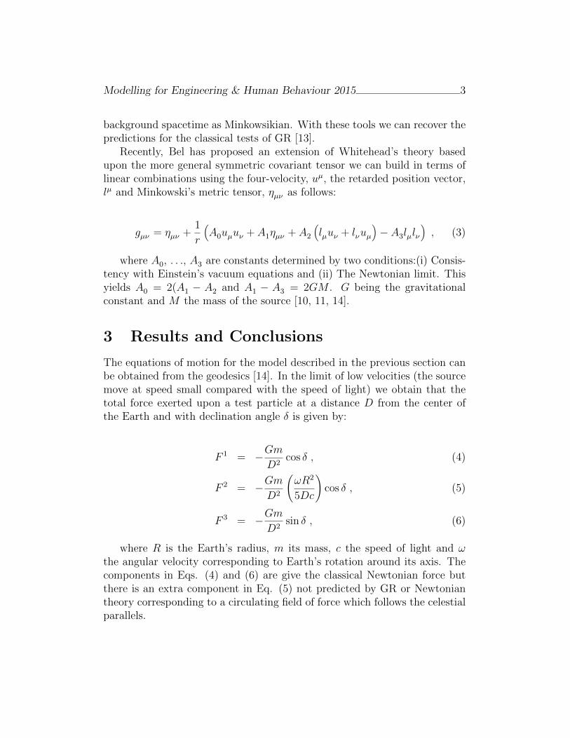
3 Results and Conclusions
The equations of motion for the model described in the previous section canbe obtained from the geodesics [14]. In the limit of low velocities (the sourcemove at speed small compared with the speed of light) we obtain that thetotal force exerted upon a test particle at a distance D from the center ofthe Earth and with declination angle δ is given by:
F 1 = −GmD2
cos δ , (4)
F 2 = −GmD2
(ωR2
5Dc
)cos δ , (5)
F 3 = −GmD2
sin δ , (6)
where R is the Earth’s radius, m its mass, c the speed of light and ωthe angular velocity corresponding to Earth’s rotation around its axis. Thecomponents in Eqs. (4) and (6) are give the classical Newtonian force butthere is an extra component in Eq. (5) not predicted by GR or Newtoniantheory corresponding to a circulating field of force which follows the celestialparallels.

Modelling for Engineering & Human Behaviour 2015 4
Although the Newtonian forces acting upon a rigid spherical body cannotmodify its angular momentum, it can be shown that the circulating field inEq. (5) allows for a transfer of energy and angular momentum from the Earthto the spacecraft or viceversa providing a mechanism to explain the reportedflyby anomalies. For a quantitative analysis of the predictions compared withthe observations for six flybys the interested reader is referred to Ref. [14].
References
[1] J. D. Anderson, J. K. Campbell, J. E. Ekelund, J. Ellis, J. F. Jordan,Anomalous orbital-energy changes observed during spacecraft flybys ofthe Earth, Phys. Rev. Lett. 100 (2008) id. 091102.
[2] L. Iorio, A flyby anomaly for Juno ?. Not from standard physics, Adv.Space Res. 54(11) (2014) 2441-45. arXiv:1311.4218
[3] C. Lammerzahl, O. Preuss, H. Dittus, Is the physics of the Solar Systemreally understood ? in Lasers, Clocks and Drag-Free Control, Astrophys.and Space Science Library 349 (2008) 75-101. arXiv:gr-qc/0604052
[4] L. Iorio, The effect of General Relativity on hyperbolic orbits and itsapplicatioin to the flyby anomaly, Scholarly Research Exchange 2009,id. 807695, 1-8.
[5] S. L. Adler, Can the flyby anomaly be attributed to earth-bound darkmatter ?, Phys. Rev. D 79 (2009) 023505. arXiv:0805.2895v4
[6] L. Acedo, The flyby anomaly: A case for strong gravitomagnetism ?,Adv. Space Res. 54 (2014) 788-796. arXiv:1505.06884
[7] M. J. Pinheiro, The flyby anomaly and the effect of a topological torsioncurrent, Phys. Lett. A 378 (2014) 3007-11.arXiv:1404.1101
[8] K. Wilhelm, B. N. Dwivedi, Anomalous Earth flybys of spacecraft, As-trophys. Space Sci. 358(18) (2015) 1-8.
[9] List of unsolved problems in physics, Wikipedia,https://en.wikipedia.org/wiki/List of unsolved problems in physics
(accessed November 18th, 2015).

Modelling for Engineering & Human Behaviour 2015 5
[10] Ll. Bel, A look inside the theory of the linear approximation, arXiv:gr-qc/0605057v3, 2007.
[11] Ll. Bel, A new look inside the theory of the linear approximation:Gravity assists and Flybys, unpublished paper. Available online athttp://www.lluisbel.com/upload/OnHold/FlyBys.pdf, 2015.
[12] A. N. Whitehead, The Principle of Relativity, Cosimo, Inc., New York,2007.
[13] A. J. Coleman, Whitehead’s principle of Relativity,arXiv:physics/0505027v2, 2005.
[14] L. Acedo, The flyby anomaly in an extended Whitehead’s theory, Galax-ies 3, 2015, 113-128.
Supply schedule in intermittent water supplybased on quantitative and qualitative criteria
A. E. Ilaya-Ayza ∗, R. Perez-Garcıa,J. Izquierdo, and J. Benıtez
Fluing-Instituto de Matematica Multidisciplinar (IMM)
Universitat Politecnica de Valencia,
Camino de Vera SN, pc: 46015, Valencia, Spain
November 30, 2015
1 Introduction
Intermittent water supply (IWS) is a form of access to water in which thewater is supplied only a few hours per day. This leads to problems of equityof supply [1, 2], infrastructure deterioration [3] and water quality [4]. Despitethese problems, IWS is very common in developing countries [5], where con-tinuous supply is very difficult due to insufficient funding, physical scarcityor mismanagement [6].
Generally, water companies that manage IWS have reduced economicresources. Therefore, proposals to improve the system performance must bebased on alternatives that involve reduced human and economic resources.
If the network is not sectorised, IWS is simultaneous for all users. Whenthe network is sectorised, sectors have non-simultaneous delivery schedules.
One problem of IWS is the peak flow occurring at certain times of day.This value is usually greater than the peak flow in a system with continuouswater supply (CWS). This reduces pressure and flow at the ends or highpoints and causes inequity in the supply and complaints from users.
∗e-mail: [email protected]
6
Modelling for Engineering & Human Behaviour 2015 7
Reorganizing supply schedules based on qualitative and quantitative tech-nical criteria reduces the peak flow and consequently improves pressures.
Water company experts’ opinion is very important in the optimizationprocess. Thus, pairwise comparison matrices defined in the Analytic Hierar-chy Process (AHP) [7] method are used to quantify this opinion.
2 The Proposed Methodology
In an IWS the pattern of supply tends to be constant by the presence ofhousehold deposits. Large flows occur in the first minutes but they arereduced at the end of the delivery period. The flow variation is not large,ranging from 20% to 30%. Therefore, it can be simplified by calculating theaverage volume per delivery period (Vs) [8] or supply blocks.
V sj =daily volume supplied to sectorsj
number of supply hours.
The optimization process assigns a new schedule to these supply blocksbased on the defined technical requirements. In this paper we use four crite-ria, three quantitative and one qualitative.
Pressure (C1): sectors with lower operating pressure are those that canchange their schedule, and users with lower pressure accept the measurestaken to improve their conditions of service. Number of users (C2): themore users the sector have, the lower the possibility of modifying its supplyschedule. The aim is to improve the service and reduce the number of peopleaffected by the change. Supply hours (C3): the sectors that have fewer supplyhours have greater flexibility in assigning a new schedule.
The qualitative criterion is related to the ease of operation of the sector(C4). It depends on various factors: the availability of sectorisation valves,their proper performance, their accessibility, the working difficulty for oper-ators, the mainly manual operation, complaints from the users, and others.Thus, this qualitative variable is consulted to experts from the water com-pany with the AHP methodology. The weight of this variable in every sectoris the normalized geometric mean of the eigenvectors of the pairwise com-parison matrices of each expert. Experts are also consulted to establish theweight of each criterion. Then the weight associated to number of users(wuj), pressure (wpj), supply hours (whj), and ease of operation (woj) foreach i sector are calculated. These weights are used in the objective function.
Modelling for Engineering & Human Behaviour 2015 8
We use integer linear programming (LP) with binary variables. As a resultof the optimization process we obtain an m × n matrix of binary variablesV = (vkl), where m is the number of hours of a day, and n is the total numberof sectors. A value of 1 in the matrix indicates the start of the supply periodof the sector.
To reallocate supply schedules in a block (all supply period), we proposeto use the m×m schedule square matrix U (j) = ukl, where
ukl =
1 k = 1, . . . ,m ∧ l = k, k + 1, . . . , k + h− 1,1 if k + h− 1 > m, then l = 1, 2, . . . , k + h− 1−m,0 otherwise.
to calculate supply schedule vectors for each sector j:
Xj =
(m∑i=1
viju(j)i1 ,
m∑i=1
viju(j)i2 , . . . ,
m∑i=1
viju(j)im
)= (x1j, x2j, . . . , xmj).
Multiplying the hourly volume V sj by the supply schedule vector Xj
correspondingly, we obtain the volume delivered to each sector in the corre-sponding period represented by vector Bj.
Bj = V sj · (x1j, x2j, . . . , xmj) = (b1j, b2j, . . . , bmj).
To start with an initial priority in the current schedule for each sector,we propose an m× n matrix S = (sij) where sij = 1 for an hour with watersupply and sij = 0 for an hour without water supply. We must include inthe objective function the information of volume entering the tank per hour.The normalized value is ti. The hour in which more water enters the tankis prioritized. There is also the possibility of sectors operating in cascade.Therefore, we consider the supply hour six and supply volume xiy of thesector in cascade.
These elements allow us to configure the optimization problem.
Maximizem∑i=1
n∑j=1
(wpj + wuj + whj + woj + sij)xij + tin∑
j=1
xij + six · xiy
Subject to
m∑i=1
vij = 1 ∀ j;n∑
j=1
xkj ≤ SS ∀ k;n∑
i=1
bki ≤ VS ∀ k.
The first constraint forces one supply period per sector. In the second con-straint the number of sectors that can work simultaneously, SS, is limited.
Modelling for Engineering & Human Behaviour 2015 9
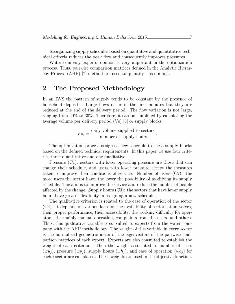
The output volume of the tank, V S, is the most important constraintin the optimization process. This value allows us to rearrange the supplyschedule of each sector and to find scenarios with better service conditions.
Figure 1: Supply schedule of each sector, Oruro south subsystem
3 Example of implementation
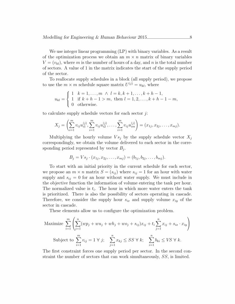
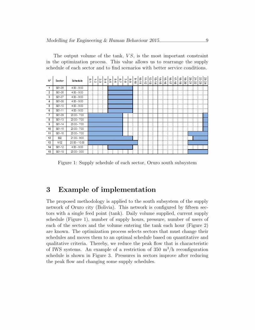
The proposed methodology is applied to the south subsystem of the supplynetwork of Oruro city (Bolivia). This network is configured by fifteen sec-tors with a single feed point (tank). Daily volume supplied, current supplyschedule (Figure 1), number of supply hours, pressure, number of users ofeach of the sectors and the volume entering the tank each hour (Figure 2)are known. The optimization process selects sectors that must change theirschedules and moves them to an optimal schedule based on quantitative andqualitative criteria. Thereby, we reduce the peak flow that is characteristicof IWS systems. An example of a restriction of 350 m3/h reconfigurationschedule is shown in Figure 3. Pressures in sectors improve after reducingthe peak flow and changing some supply schedules.
Modelling for Engineering & Human Behaviour 2015 10
Figure 2: Volume entering the tank and IWS current supply curve
4 Conclusion
Supply schedule management does not seek to perpetuate IWS. It is intendedas a short-term technical management solution, which seeks to improve theconditions of service and therefore improve quality of life. It is also a usefultool for a gradual transition from IWS to CWS.
Solutions to make IWS systems work better don’t necessarily require theconstruction of new infrastructure. IWS systems with insufficient fundinghave few economic resources. Solutions must be found based on existinginfrastructures and demanding minimal human and economic resources.
As a part of the LP problem, we propose the use of schedule matrices,which play an important role in the solution. They allow change the sectorschedule in blocks. Therefore, they are very useful for this kind of problems.
References
[1] K. Vairavamoorthy and K. Elango. Guidelines for the design and controlof intermittent water distribution systems, Waterlines, 21: 19–21, 2002.
[2] K. Vairavamoorthy, S. D. Gorantiwar, and A. Pathiranaa. Managingurban water supplies in developing countries; Climate change and waterscarcity scenarios, Physics and Chemistry of the Earth, 33: 330–339,2008.

Modelling for Engineering & Human Behaviour 2015 11
Figure 3: Optimizing supply schedules with constraint V S = 350 m3/h
[3] B. Charalambous. The Effects of Intermittent Supply on Water Dis-tribution Networks, Water Loss 2012 Conference, Manila, Philippines,2012.
[4] E. Kumpel and K. L. Nelson, Comparing microbial water quality in anintermittent and continuous piped water supply, Water Research, 47:5176–5188, 2013.
[5] C. Van den Berg and A. Danilenko, The IBNET Water Supply andSanitation Performance Blue Book. Washington D.C., The World Bank,2011.
[6] N. Totsuka, N. Trifunovic, and K. Vairavamoorthy, Intermittent urbanwater supply under water starving situations, 30th WEDC InternationalConference, Vientiane, Lao, 2004.
[7] T. L. Saaty and L. Vargas, Models, Methods, Concepts & Applicationsof the Analytic Hierarchy Process. New York, Springer, 2012.
[8] J. A. Cabrera-Bejar and V. G. Tzatchkov, Inexpensive Modeling of In-termittent Service Water Distribution Networks, World Environmentaland Water Resources Congress, 2009.
Internal Lubricant Content in inhalationCapsules
G.Ayala[∗, F. Dıez†, M.T.Gasso‡ and B.E. Jones\
([) Department of Statistics and O.R. University of Valencia
Avda. Vicent Andres Estelles, 1, 46100-Burjasot (Spain),
(†) Qualicaps Europe,
Qualicaps Europe S.A.U. 28108 Spain,
(‡) Institute of Multidisciplinar Mathematics and Department of Mathematics
Polythecnical University of Valencia, Camino de Vera s/n 46022. Valencia (Spain),
(\) School of Pharmacy & Pharmaceutical Sciences, Cardiff University, Cardiff, UK.
November 30, 2015
1 Introduction
Hard capsules are manufactured in a continuous process on large automatic ma-chines, see Figure 1. They are formed on stainless steel mould pins mountedin-line onto metal strips (bars). There are different sets of bars to make the capsand bodies of each size of capsule. Groups of bars are dipped in to a temperaturecontrolled container, called a dip pan, containing a warm aqueous solution ofthe polymer, either gelatin or hypromellose (HPMC). Films are formed on themould pins most commonly by a gelation process that relies on the temperaturedifference between the cold pin and the hot solution. This is an inherent propertyof gelatin solutions and HPMC solutions are formulated to gel by the addition ofa network former such as carrageenan and potassium chloride as a promoter [2].The bars are raised out of the dip-pan and are rotated end over end to improvethe film distribution on the pins as they are transferred from the lower level ofthe machine to the upper one. At this point the films have set and are no longermobile. Groups of bars are moved by hydraulic pushers through a series of dryingkilns, which use large volumes of controlled humidity and temperature to dry thefilms. At the end of the upper level the bars are transferred to the lower level and
∗[email protected];[email protected]; [email protected],[email protected]
12
Modelling for Engineering & Human Behaviour 2015 13
Figure 1: Capsules manufacturing ( From Qualicaps Europe).
are moved back to the front-end of the machine. When the pins emerged fromthe kilns they are dried to a level of >16.0%, which is just above the upper levelof the standard moisture content specification. These dried films adhere stronglyto the pins. The next part of the process is to strip them from the pins usingmetal jaws. The internal lubricant content (ILC) is a critical factor enabling thisto occur without capsule damage. If insufficient is used the capsule shells willsplit during removal. Pairs of bars, one cap and one body are selected from eachside of the machine and enter into the automatic section. The lubricant is apropriety mixture pharmaceutical grade excipients and is different for each cap-sule manufacturer and their compositions are registered in the companies DrugMaster File. Lubricant is loaded into a pump, the flow rate from which can beadjusted using a pressure valve. The lubricant is applied to a circular foam rollerthat transfers a sufficient quantity to the pins as they pass underneath. The pinbars are moved towards the centre of the machine and the pins are inserted intorotating circular tubes lined with a felt pad. These clean the pins and spread thelubricant evenly over their surface. These pads are changed at regular intervalsto avoid a build-up and saturation with the lubricant [1, 2, 3, 4, 5].
Several papers have described the influence of ILC on aerosolization [6, 7].The reference [7] showed that there is an optimum ILC range to obtain goodpowder release from capsules as measured by their emitted dose and fine particlefraction [7]. They suggested that the effect could be related to the roughness ofcapsule internal surface.
2 Results
The experts have evaluated the most important factors in the process control.Our study have two main goals. Firstly, the evaluation of which of these factorsare important i.e. their effects are relevant for the response variable, internal lu-bricant content (ILC from now on). Our experimental design has two categoricalfactors (pump flow and pin location) and one numeric covariable (time) with asample size of 432 corresponding to three levels for each experimental factors, 24
Modelling for Engineering & Human Behaviour 2015 14
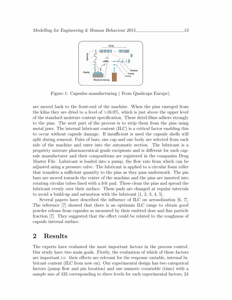
Figure 2: Observed means for different pump flows: low (solid line), medium(dashed line) and high (dotted line).
instants for the covariable time and two replications. The statistical analysis wasperfomed using the software environment R. We evaluate if there are significantfactors or if there exists any relevant interaction between them. All pairwise com-parisons of means and variances for each categorical factor have been performedand the results appears in table 1.
Table 1: Comparison of means (t-test) and variances(F-test)Dif. 95% CI p1 Ratio 95% CI p2
Pump flow 1-2 -16.66 [-20.14,-13.18] 0.00 0.61 [0.44,0.85] 0.002-3 -1.69 [-5.56,2.17] 0.39 1.00 [0.72,1.40] 0.981-3 -18.35 [-21.83,-14.88] 0.00 0.62 [0.45,0.86 ] 0.00
Location Bar4-Pi1 -9.43 [-13.12,-5.73] 0.00 0.74 [0.53,1.03] 0.07Pi1-Pi28 -2.32 [-6.47, 1.83] 0.27 0.84 [0.60,1.17] 0.29Bar4-Pi28 -11.75 [-15.64,-7.85] 0.00 0.62 [0.45,0.86] 0.00
A full factorial linear model have been fitted. A variable selection was ap-plied using and stepwise approach in order to minimize the Akaike informationcriterium. The final selected model has only the main effects (for pump flow andlocation) and two interaction, pump flow with time and pump flow with location.
Secondly, a functional data approach has been used. The response is now theobserved ILC along time and the predictors are pump flow and location. Themean functions for different pump flows (respectively locations) were comparedusing a functional anova. Significant differences are observed for pump flow factorbut not for location.

Modelling for Engineering & Human Behaviour 2015 15
Acknowledgements
This research was supported by Qualicaps Europe, S.A.U.; Spanish DGI Grantno. MTM2014-58159-P (M.T. Gasso) and G. Ayala (DPI2013-47279-C2-1-R).
References
[1] B.E. Jones. Quali-V R©-I: a new key for dry powder inhalers. Drug DeliveryTechnology, 3(6):52–57, 2003.
[2] B.E. Jones. Manufacture and properties of two- piece hard capsules, pages79–100. In: Podczeck, F., Jones, B.E. (Eds), Pharmaceutical Press, London,2nd edition, 2004.
[3] B.E. Jones. The evolution of DPI capsules. Inhalation, 2(6):20–23, 2008.
[4] S. Nagata. Advantages to HPMC capsules. A new generation’s hard capsule.Drug Deliv. Technol., 2:32–42, 2002.
[5] T. Ogura, Y. Furuya, and S. Matsuura. HPMC capsules , an alternative toGelatin. Pharm. Technol. Eur., 10:32–42, 1998.
[6] S. Saim and S.T. Horhota. Process for overcoming drug retention in hardgelatin inhalation capsules. Drug development and industrial pharmacy, 28:641–654, 2002. doi: 10.1081/DDC-120003855.
[7] I.Y. Saleem, F. Diez, B.E. Jones, N. Kayali, and L. Polo. Investigation onthe aerosol performance of dry powder inhalation hypromellose capsules withdifferent lubricant levels. International Journal of Pharmaceutics, 492(1-2),258 – 263, 2015. doi: http://dx.doi.org/10.1016/j.ijpharm.2015.07.034.
Microscopic and macroscopic models for gasleak detection
Fidel Aznar[ ∗, Mar Pujol[, and Ramon Rizo[
([) Department of Computer Science and Artificial Intelligence.
University of Alicante, San Vicent del Raspeig, Alicante (E-03080). Spain
November 30, 2015
1 Introduction
Fracking for natural gas and oil extraction significant leaks of methane, a po-tent greenhouse gas. This extraction technique proliferate across world, andscientists are raising questions about whether millions of gallons of contam-inated drilling fluids could be threatening water supplies, affecting humanhealth and increasing greenhouse effects.
Currently, many companies are using methane-leak detection tools, suchas infrared cameras, that are too labor-intensive and fail to find many sources.Researchers are developing more sensitive methane sensors for leak detectionthat utilize cavity ring-down spectroscopy (CRDS). These sensors can dis-cern between oil-and-gas-related methane emissions and those from biogenicsources, such as cattle. A principle advantage of the sensor is its simple de-sign, which allows for a lighter weight and less expensive, less complicatedsystems. This makes the sensor suitable for large-scale deployment in bothstationary systems and unmanned aerial vehicle and drone applications.
One of these applications is presented in [1], where a methane sensormounted on a remotecontrolled aircraft is developed. The aircraft was usedto quantify emission rates from well pads and a compressor station in Texas,
∗Contact author mail: [email protected]. This work has been supported by the SpanishMinisterio de Economia y Competitividad, project TIN2013-40982-R
16

Modelling for Engineering & Human Behaviour 2015 17
USA. In another paper presented in [2], a drone have been used for de-tecting fugitive methane emissions. Althought currently there are severalapplications of UAV for methane detection we have not found specific swarmbehaviours for this task, which is specially relevant for large area navigationand data recollection.
2 Microscopic behaviour
In this paper we will present a swarm behaviour, which monitors gas leaks byusing a swarm of homogeneous UAV. Thus, this system is fully distributed,scalable and highly fault tolerable. Our main goal, once the behaviour isdesigned, is to determine the ability of the swarm to locate, converge andfollow a gas leak. Therefore, a macroscopic model to predict the globalbehaviour of the swarm and to verify its performance will be specified. Morespecifically, we propose a homogeneous behaviour, executed by all agents,consisting of two states. Initially, drones look for any trace of the leak in theenvironment. Once the leak is detected, the drone will head to it. Then, thedrone will try to stay in its perimeter. The initial state is Discover, sincewe initially assume that the position of the leak is unknown. The transitionfrom Discover state is performed when the agent’s methane sensor detects aleak. In this case, the new state will be Gas.
vD(t) = vD(t− 1) + rand · µ1
vG(t) =∥∥∑
s∈S ((pos(s)− pos(rob)) · s)∥∥+∥∥∥∑|R|
i=1(pos(ri)− pos(rob))∥∥∥+ rand · µ2
Where vD and vG define the velocity to be executed in the Discover andGas behaviours respectively. µ parameters define the importance of randomperturbations for discovering and action executions using a gaussian randomgenerator with mean 0 and variance 1. S is a set that contains the mostintense readings for our methane sensor in a period of 1 minute. R is a setthat contains all the swarm drones.
Modelling for Engineering & Human Behaviour 2015 18
3 Macroscopic behaviour
In this work, we consider the framework proposed in [4] in order to obtainthe probability distribution of the swarm position for any time t. This willenable us to predict, in great detail, the behaviour of the overall system.As described by [4], once the microscopic behaviour has been defined, theglobal behaviour of the system can be calculated using the Fokker-Planckequation. This equation provides a method to statistically model a swarmof robots based on modelling techniques of multi-particle systems from thefield of quantum physics. From a Langevin equation, that represents thebehaviour of a single particle, the Fokker-Planck equation is derived for allthe system.
∂ρ(r, t)
∂t= −∇ (A(r, t)ρ(r, t)) +
1
2Q∇2
(B2(r, t)ρ(r, t)
)(1)
As we have already seen in [3], the FokkerPlanck equation implements thenecessary abstraction of microscopic details as described above and treatsrapidly-changing parameters such as noise. It is important to underline thatthe equation is still exact if this noise is generated by a Gaussian process, thatis, if it is fully determined by the first two moments. It gives the temporalevolution of the probability density describing the positions of the agents.
A function determines the displacement of the swarm. A depends pri-marily on a vector representing the directional information. A potential fieldP is commonly used to define it. In our case, we need to establish a functionthat takes into account the following things based on the proposed micro-scopic model: the random motion states of the robot; the probability thata movement of an agent fails in its execution (e.g. due to a collision); andthe potential field where the robots move. Although it is possible to modela probability distribution for each state, as our microscopic model has nointeraction between agents (except purely physical, as collisions) and the be-haviour of states is relatively simple, the macroscopic behaviour of the swarmcan be comprised in a single distribution.
A = γ∇mleak(r, t)
||∇mleak(r, t)||v (2)
Where γ is a normalization term and mleak is a potential field obtaniedfrom the expected leak evolution through the environment.

Modelling for Engineering & Human Behaviour 2015 19
Function B describes the nondeterministic motion and, therefore, it takesinto account the random motion of agents. Two forces, that must be con-sidered, take part in the microscopic behaviour. On the one hand, someinfluences derived from agents that are on Discover and Gas states. On theother hand, the behaviour itself causes that the environment has areas witha higher density of agents. In these areas the probability of collision can beincreased depending on the density of agents at a given time.
4 Experimentation
The simulation of the microscopic model has been developed using the soft-ware MASON. We use a swarm of 100 agents randomly distributed by theenvironment that moves uniformly at 60km/h. The simulation uses smallsize drones (< 3m2) and a environment size of 1km2.
We have carried out 200 random leak tests through the environment toverify the correct operation of our model at local level. Initially, we checkthe convergence of the swarm for a single static leak. We obtain that all therobots stay within the gas leak or in their perimeter (distance to the leak < 10meters) 98% of the tests. Next, using a gas leak simulation tools we verify deconvergence of the swarm with several active leaks (that change and evolveeach simulated time step) with another 200 tests. For this experimentationwe simulate variable winds from 0 to 5m/s. In this case we found that 78%of the times one or more drones are able to detect and follow the leak.
5 Conclusions
Taking into account the properties of methane emissions we have presenteda microscopic model for a swarm of drones, capable of monitoring these leaksproperly. We have also provided a macroscopical model, based on Fokker-Planck equations that can be used to predict the overall evolution of theswarm. This mathematical model will calculate the likelihood of an agent tobe placed in a position at a given time. The experimental results presentedshow the proper evolution of our system and their ability to detect and followa simulated gas leak.
Modelling for Engineering & Human Behaviour 2015 20
References
[1] Amir Khan, David Schaefer, Lei Tao, David J. Miller, Kang Sun, MarkA. Zondlo, William A. Harrison, Bryan Roscoe and David J. Lary. LowPower Greenhouse Gas Sensors for Unmanned Aerial Vehicles. RemoteSens. 2012, 4, 1355-1368.
[2] Kathryn McKain, Adrian Down, Steve M. Raciti, John Budney, Lucy R.Hutyra, and Cody Floerchinger, Scott C. Herndon, Thomas Nehrkorn,Mark S. Zahniser, Robert B. Jackson, and others. Methane emissionsfrom natural gas infrastructure and use in the urban region of Boston,Massachusetts. Proceedings of the National Academy of Sciences, 2015,12 (7), 1941-1946.
[3] Heiko Hamann. Space-Time Continuous Models of Swarm Robotic Sys-tems: Supporting Global-to-Local Programming, volume 9. Springer, 2010.
[4] Heiko Hamann and Heinz Worn. A framework of space–time continuousmodels for algorithm design in swarm robotics. Swarm Intelligence, 2(2-4):209–239, 2008.

Modelling for Engineering & Human Behaviour 2015____________________________21
Modelling the survival of the Spanish construction SME in a crisis
environment
Isabel Barrachina; Elena De la Poza.
Centro de Ingeniería Económica
Universitat Politècnica de València
Abstract
The construction sector headed the Spanish economy during the blooming period 1998-2007;
its direct contribution to the Spanish economic growth amounts over the 20% in annual terms.
The turmoil of the financial sector impacted the Spanish construction companies, mainly due
to their high indebtedness levels combined with the credit shortage from the banking system
to units, sellers and buyers. As a result a relevant number of construction companies declared
in bankruptcy producing a dominos effect impacting the whole Spanish economy. In this
context, taking into account financial-economic information we classify the small medium
sized construction companies by their financial distress levels (solvent; on risk of default).
Then, after identifying those companies which survived to the economic recession we model
the processes of survival of the Spanish SME to find out possible financial-economic patterns
that explain their continuity and to propose guidelines to strategy decision makers.
Keywords: survival; financial distress; construction sector; SME.
1. Introduction
The construction sector in Spain experienced a large expansion since 2000 becoming the main engine of the Spanish economy, (ICE, 2009).
There was an increase in housing prices and unprecedented growth of mortgage debt.
The global economic crisis (2008) caused a decline in mortgage approvals granted by banks it led to a clear increase of developers and construction companies declared bankrupt. However, some companies achieve to survive the financial downsize.
The primary goal of this study is to identify the strategies followed by the Spanish
construction companies on default risk at the beginning of the economic recession that
managed to survive. Also, the specific objectives are:
- Develop a descriptive analysis of Spanish construction companies and its trend
throughout the period of crisis [2008, 2013]
-Classify the enterprises in 2008 according to their economic-financial risk
-Analyze the survival capability of companies.
Modelling for Engineering & Human Behaviour 2015____________________________22
2. Methods
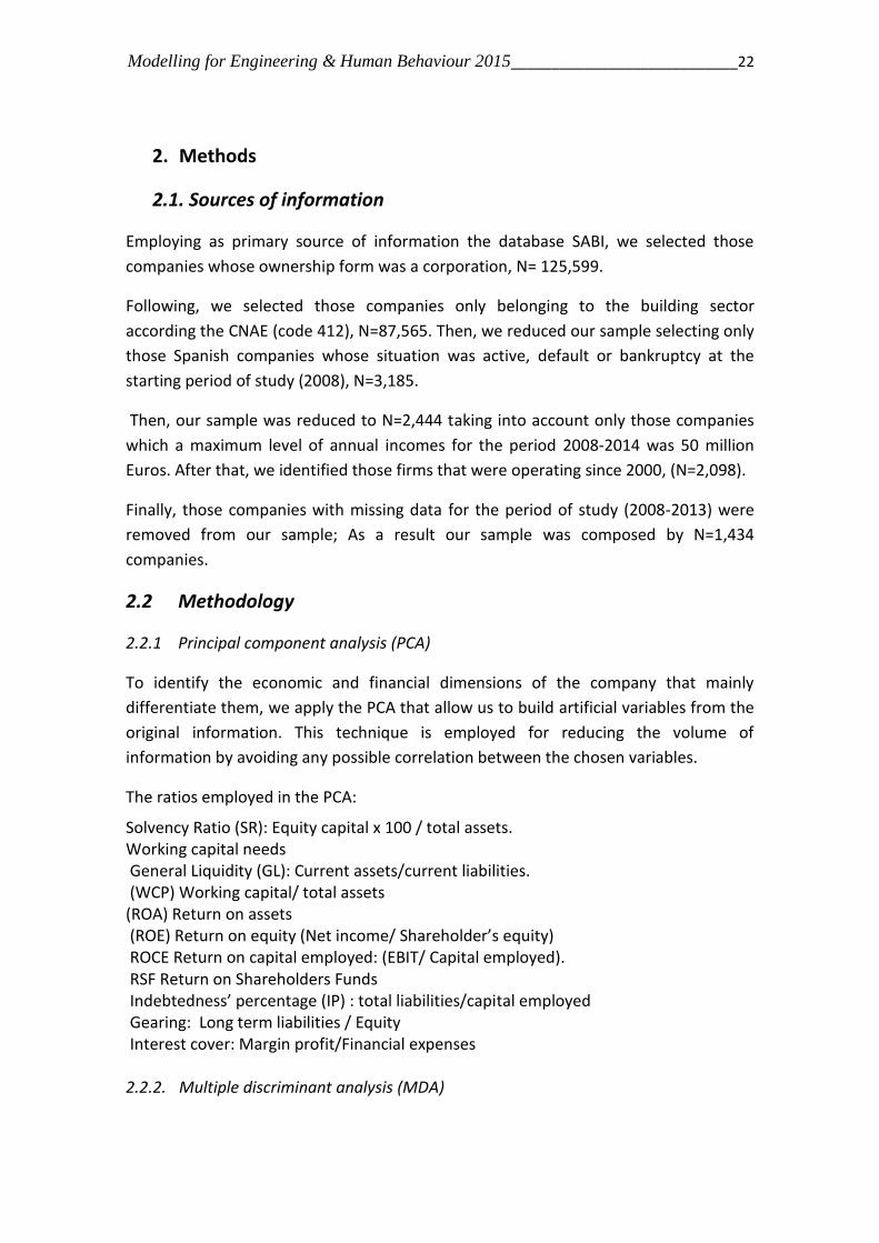
2.1. Sources of information
Employing as primary source of information the database SABI, we selected those
companies whose ownership form was a corporation, N= 125,599.
Following, we selected those companies only belonging to the building sector
according the CNAE (code 412), N=87,565. Then, we reduced our sample selecting only
those Spanish companies whose situation was active, default or bankruptcy at the
starting period of study (2008), N=3,185.
Then, our sample was reduced to N=2,444 taking into account only those companies
which a maximum level of annual incomes for the period 2008-2014 was 50 million
Euros. After that, we identified those firms that were operating since 2000, (N=2,098).
Finally, those companies with missing data for the period of study (2008-2013) were
removed from our sample; As a result our sample was composed by N=1,434
companies.
2.2 Methodology
2.2.1 Principal component analysis (PCA)
To identify the economic and financial dimensions of the company that mainly
differentiate them, we apply the PCA that allow us to build artificial variables from the
original information. This technique is employed for reducing the volume of
information by avoiding any possible correlation between the chosen variables.
The ratios employed in the PCA:
Solvency Ratio (SR): Equity capital x 100 / total assets. Working capital needs General Liquidity (GL): Current assets/current liabilities. (WCP) Working capital/ total assets (ROA) Return on assets (ROE) Return on equity (Net income/ Shareholder’s equity) ROCE Return on capital employed: (EBIT/ Capital employed). RSF Return on Shareholders Funds Indebtedness’ percentage (IP) : total liabilities/capital employed Gearing: Long term liabilities / Equity Interest cover: Margin profit/Financial expenses 2.2.2. Multiple discriminant analysis (MDA)

Modelling for Engineering & Human Behaviour 2015____________________________23
In order to find the mathematical model that better discriminate the companies into
two groups (default risk companies at year (n+1) versus no- risk companies at year
(n+1)) by their financial ratios estimates at year n. Hypothesis: the companies are on
default’s risk when their solvency ratio is lower than 1.5 (Amat, 2008).
2.2.3. Survival analysis
The reason to employ survival analysis is the necessity to take into account the variable
time (since other regression techniques such as the logistic regression does not) when
studying the behavior of companies. In particular, we want to identify the time that
takes for a company declare in default as a result of its economic-financial trend.
We chose Kaplan-Meier, a non-parametric estimate of the survival function. This
methodology is commonly used to describe survivorship of study population/s by a
intuitive graphical presentation.
This method calculates the probability of survival every time a company suffers the
event of bankruptcy, from the number of companies that are subject to bankruptcy
due to the crisis. The factor that differentiates one business from others is the initial
classification of companies according to their forecasted risk of default next year
3. Results
3.1 Descriptive Analysis and PCA results
At 2008, the starting year of the study, the 85% firms of our sample were functioning
(Total N=1,434). While at the end of the period of study (2013), the number of
companies operating was amounted to 1,210 which implies a drop of 15.6%. Derived
from the application of the PCA technique the variables ROE, IP, LP and WCP were
those with greater discriminant power, (Cohen et al., 2003)
3.2. MDA Results
Table 1 shows the standardized canonical discriminant Function coefficients with the
variables that better discriminate our sample into two groups: default companies at
(n+1) versus those that are not. The analysis diagnoses correctly the 77,8% companies.
Table 1.
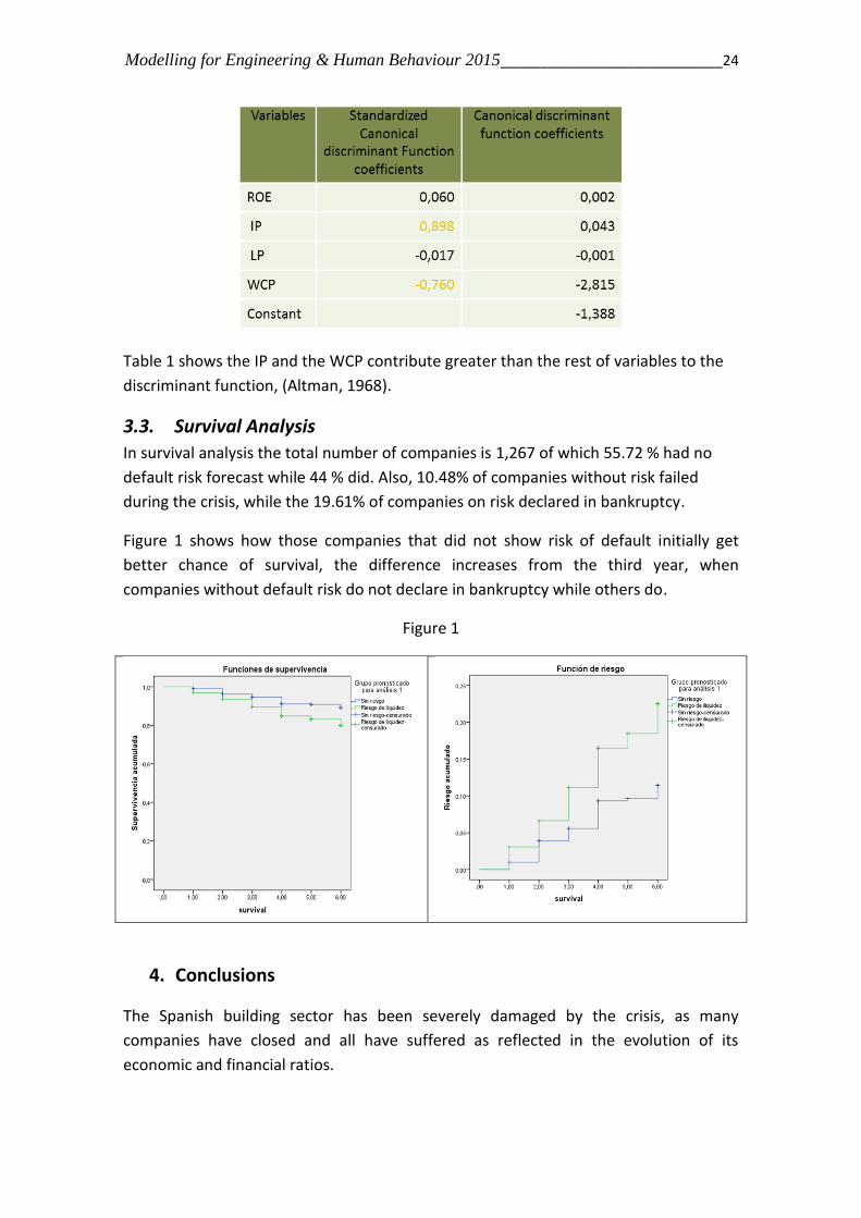
Modelling for Engineering & Human Behaviour 2015____________________________24
Table 1 shows the IP and the WCP contribute greater than the rest of variables to the
discriminant function, (Altman, 1968).
3.3. Survival Analysis
In survival analysis the total number of companies is 1,267 of which 55.72 % had no
default risk forecast while 44 % did. Also, 10.48% of companies without risk failed
during the crisis, while the 19.61% of companies on risk declared in bankruptcy.
Figure 1 shows how those companies that did not show risk of default initially get
better chance of survival, the difference increases from the third year, when
companies without default risk do not declare in bankruptcy while others do.
Figure 1
4. Conclusions
The Spanish building sector has been severely damaged by the crisis, as many
companies have closed and all have suffered as reflected in the evolution of its
economic and financial ratios.

Modelling for Engineering & Human Behaviour 2015____________________________25
The MDA shows the variables that more influence on the firm’s default risk are the
working capital firms’ percentage.
The MDA is a useful tool to predict the companies on risk to failure since classifies
correctly about the 92% of companies of the sample.
Throughout this study it has been determined that the chances of survival of
companies in a crisis environment decrease if the initial situation is of risk especially
from the third year of crisis environment.
During the monitoring period 10.48% SME that initially were not classified as risk of
default declared in bankruptcy especially during the first three years, and 19.61% of
companies classified as default risk.
The difference between the chances of survival between the two groups of firms
increases from the third year. 50% of the companies that survive the crisis whose
initial situation was risky do in a bad financial economic situation, while the other half
significantly improve their ratios.
Preliminary results show that its main strategy seems to be to improve the state of
liquidity through debt restructuring and the decrease in financial expenses due to
lower interest rates.
References
Altman, Edward I. (1968): “Financial ratios, discriminant analysis and the prediction of
corporate
Amat, Oriol (2008): “Análisis de Estados Financieros. Fundamentos y aplicaciones”
Información Comercial Española, ICE: Revista de economía, ISSN 0019-977X, Nº 850,
2009 (Ejemplar dedicado a: La primera crisis global: procesos, consecuencias, medidas)
, págs. 23-40
Cohen, J., Cohen, P. C., West, S. G., & Aiken, L. S. (2003). (3rd Ed.) Applied multiple
regression/correlation analysis for the behavioral sciences. Mahwah, NJ.: Lawrence
Erlbaum.
SABI Database [Last access: July 2015].
An algorithm for quasi-linear control problemsin the economics of renewable resources: Thesteady state and end state for the infinite and
long-term horizon.
L. Bayon1∗, P.J. Garcıa-Nieto1, R. Garcıa-Rubio2,J.A. Otero1 and C. Tasis1
(1) Department of Mathematics, University of Oviedo, Spain
(2) Department of Business & Administration, University of Salamanca, Spain
1 Introduction
This paper presents the problem of finding the optimal harvesting strategy(see [1], [2] and [3]), maximizing the expected present value of total revenues.The problem is formulated as an optimal control problem [4]. Combining thetechniques of Pontryagin’s Maximum Principle and the shooting method,an algorithm has been developed that is not affected by the values of theparameter. The algorithm is able to solve conventional problems as well ascases in which the optimal solution is shown to be bang-bang with singulararcs. In addition, we present a result that characterizes the optimal steady-state in infinite-horizon, autonomous models (except in the discount factor)and does not require the solution of the dynamic optimization problem. Wealso present a result that, under certain additional conditions, allows us toknow a priori the final state solution when the optimization interval is finite.Finally, several numerical examples are presented to illustrate the differentpossibilities of the method.
∗e-mail: [email protected]
26

Modelling for Engineering & Human Behaviour 2015 27
2 Statement of the problem
For the study of the economics of a renewable resource [2], we shall first seethe pattern of biological growth of the resource. In this paper, we considerthe growth function for a population of some species of fish. We assume thatthis fishery has a intrinsic growth rate denoted by r, which represents thedifference between the population’s birth and natural mortality rates. Let usassume that the population stock is x, and the rate of change of the populationis x. A commonly used functional form is the simple logistic function:
x(t) = fl(x) = rx(t)
(1− x(t)
k
)(1)
where k is the carrying capacity of the species. In this paper, and in linewith [3], we model the dynamics of the fish stock biomass (x) when humanharvesting is included in the problem, in the more general form as:
x(t) = fl(x)− h(t) (2)
where h(t), the rate of biomass harvest, will be considered as a independentvariable. Let us now see how to model the cost functions.
Let π(x, h) be the instantaneous net revenue from the harvest of the stockbiomass:
π(x, h) = p(h)h− c(x, h) (3)
where p(h) is the inverse demand function and c(x, h), the cost functionassociated with the harvest. The functional forms for the demand and costfunctions adopted in this paper are:
p(h) = p0 − p1h (4)
c(x, h) =chα
x(5)
where h represents landings of fish and p0 and p1 are coefficients. Substituting(4) and (5) in (3), the profit function is:
π(x, h) = p0h− p1h2 −chα
x(6)
where the meaning of the parameters is: p0 is the price of the stock, p1 is thestrength of demand, c is the cost of exploitation and α is the harvest costparameter.
Modelling for Engineering & Human Behaviour 2015 28
Our model of renewable resource exploitation is an open-access fisherymodel, in which each firm takes the market price of landed fish as given.The firm’s objective is to maximize profits from the harvest schedule overan infinite time horizon, subject to the dynamic constraint equation (2) andother natural and policy restrictions that involve limits (or bounds) for theharvest, h(t), and stock, x(t). Hence, our objective is to maximize profitfrom the harvest schedule over an infinite time horizon:
maxh(t)
∫ ∞0
π(x, h)e−δtdt = maxh(t)
∫ ∞0
(p0h− p1h2 −chα
x)e−δtdt (7)
subject to:
x(t) = fl(x)− h(t); x(0) = x0 (8)
h(t) ∈ H(t); x ∈ [0, k] (9)
where δ > 0 is the discount rate, i.e. the marginal returns on capital for thecompany, and x0 is the initial stock level.
As can be seen, the stated problem (7), (8), (9) is one of Optimal Control(OC) that presents a number of noteworthy features. First, the optimizationinterval is infinite. Second, the time t is not explicitly present in the problem(time-autonomous problem), except in the discount factor. Third, we imposeconstraints on the control and, fourth, it constitutes a problem which is quasi-linear when real values are considered for the parameters.
3 Optimization Algorithm
Faced with the complication of having to use different techniques when thefunctional is linear or nonlinear in the control variable, the contribution ofour method is that it is valid in cases ranging between quasi-linearity andsingular arcs. We have used the combined techniques of Pontryagin’s Maxi-mum Principle (PMP) [4] and the shooting method to build this optimizationalgorithm. If we denote by Yx(t) the coordination function:
Yx(t) = −Fufu· e
∫ t0 fxds +
∫ t
0
Fx · e∫ s0 fxdzds (10)
the theoretical development carried out allows us to present a necessary max-imum condition.
Modelling for Engineering & Human Behaviour 2015 29
Theorem 1. A necessary maximum conditionLet u∗ be the optimal control, let x∗ ∈ C1 be a solution of the above
problem. Then there exists a constant K ∈ R such that:
If umin < u∗ < umax =⇒ Yx∗(t) = KIf u∗ = umax =⇒ Yx∗(t) ≤ KIf u∗ = umin =⇒ Yx∗(t) ≥ K
(11)
Thus, the problem consists in finding for each K the function xK that sat-isfies: xK(0) = x0, the conditions of Theorem 1 and, from among thesefunctions, the one that satisfies the transversality condition:
limt→∞
λ(t) = 0 (12)
The algorithm consists of two fundamental steps:Step 1) The construction of xK . The construction of xK can be per-
formed using a discretized version of the coordination equation: Yx(t) = K.For each K, we construct the xK , using this equation and when the valuesobtained do not obey the constraints, we force the solution to belong to theboundary until the moment established by conditions of Theorem 1.
Step 2) The calculation of the optimal K. The calculation of the optimalK could be achieved by means of an adaptation of the shooting method.Varying the coordination constant, K, we search for the extremal that fulfilsthe second boundary condition (12). Starting out from two values for thecoordination constant, K: Kmin and Kmax and using a conventional methodsuch as the secant method, our algorithm converges satisfactorily.
4 Steady-state solution
For time-autonomous problems, where the time, t, is not explicitly presentin the problem, except in the discount factor, the optimal solution is timeinvariant in the long term and converges to an equilibrium state. The methoddeveloped in [5] characterizes the optimal steady-state in single-state, infinite-horizon problems, by means of a simple function of the state variable, calledthe evolution function.
The method consider the one-dimensional, infinite-horizon problems of
Modelling for Engineering & Human Behaviour 2015 30
the form:
maxu(t)
J =
∫ ∞0
G(x(t), u(t))e−δtdt (13)
x(t) = f (x(t), u(t)) , x(0) = x0 (14)
For a steady-state solution, u = R(x), the evolution function, is defined by:
L(x) = δ
(Gu(x,R(x))
fu(x,R(x))+ W (x)
)(15)
with:
W (x) =1
δG(x,R(x)) (16)
The function L(x) serves to formulate the following necessary condition forthe location of the optimal steady state xs:
L(xs) = 0 (17)
To the best of our knowledge, the problem stated in this paper has neverbeen addressed using this approach. The necessary condition (17), for ourproblem, is:
L(xs) = δ(−πh(xs, fl(xs)) + W (xs)
)= 0 (18)
The above equation can be solved for xs, allowing us to obtain the harvestequilibrium, hs. We can thus know the steady-state solution a priori, withoutsolving the dynamic problem.
5 Long-term horizon: the end state
Inspired by the previous section, in this section we present a new resultthat allows us to calculate a priori the final value that is reached when theoptimization interval is not infinite (once again, without the need to solvethe dynamic problem). To do so, we shall use the same model as above, butwith an optimization interval [0, T ], assuming that it is long enough for thesteady state to be reached in its development. In order to obtain the result,we need to make an additional assumption: the system must be autonomous,and hence we must consider δ = 0. Let us consider the following problem:
max
∫ T
0
F (x(t), x(t)) dt = maxh(t)
∫ T
0
π(x, h)dt (19)
Modelling for Engineering & Human Behaviour 2015 31
Based on the Euler’s equation, that can be rewritten for autonomous systemsas follows:
F − xFx = cte (20)
and given that the solution for the steady state, (xs, hs) (with x = 0), may beknown a priori by means of the method explained in the previous section, thevalue of the constant, cte, present in (20) can be obtained straightforwardly:
cte = F (xs) = π(xs, hs) (21)
If we now consider the final moment, T , the two following conditions mustbe simultaneously verified at that moment, given that the end state is free:
Fx(x(T ), h(T )) = 0F (x(T ), h(T )) = cte
(22)
The first is the transversality condition corresponding to the free end state,and the second the simplified Euler equation (20). Simply solving this system,the end state (x(T ), h(T )) can be obtained straightforwardly.
References
[1] C.W. Clark, Mathematical Bioeconomics: The optimal management ofrenewable resources, Wiley, New York, 1990.
[2] R. Perman, Y. Ma, J. McGilvray and M. Common, Natural Resource &Environmental Economics, Pearson Education, Harlow, England, 2003.
[3] S. Agnarsson, R. Arnason, K. Johannsdottir, L. Ravn-Jonsen, L.K. San-dal, S.I. Steinshamn and N. Vestergaard, Comparative evaluation of thefisheries policies in Denmark, Iceland and Norway: multispecies andstochastic issues, SNF Report No 25/07, Bergen, Norway, 2008.
[4] L.S. Pontryagin, Mathematical Theory of Optimal Processes (Classics ofSoviet Mathematics), CRC Press, 1987.
[5] Y. Tsur and A. Zemel, The infinite horizon dynamic optimization problemrevisited: A simple method to determine equilibrium states, EuropeanJournal of Operational Research, 131(3): 482-490, 2001.
A polynomial expansion method based onHelmholtz equation for the Neutron Diffusion
Equation discretized by the Finite VolumeMethod
A. Bernal‡ ∗, J.E. Roman†, R. Miro‡, and G. Verdu‡
(‡) Instituto de Seguridad Industrial, Radiofısica y Medioambiental(ISIRYM),
Universitat Politecnica de Valencia, Camı de Vera s/n,
(†) Departamento de Sistemas Informaticos y Computacion,
Universitat Politecnica de Valencia, Camı de Vera s/n.
November 30, 2015
1 Introduction
The solution of the Neutron Diffusion Equation (NDE) is the easiest wayto determine the spatial distribution of the neutron flux in nuclear reactors.Although this equation is a simplification of the neutron transport equationusing the Fick’s Law [1], it is an integro-differential equation depending ontemporal and spatial terms. In reactor physics, one habitually eliminates thetemporal dependence for solving the steady state by transforming the equa-tion into an eigenvalue problem. In spite of this, geometrical discretizationand numerical methods are required to solve the spatial derivatives of theNDE.
The Finite Volume Method (FVM) can be easily applied to unstructuredmeshes and is typically used in the transport equations [2]. Moreover, the
∗e-mail: [email protected]
32
Modelling for Engineering & Human Behaviour 2015 33
FVM is feasible and suitable to be applied to the NDE [3].
One can obtain accurate results with typical algorithms of the FVM ap-plied to NDE for fine meshes, but they require high computational resources[3]. In addition, a polynomial expansion method can be used to obtain ac-curate results for coarse meshes to accelerate the calculation [4]. By meansof this method, the neutron flux is expanded in each cell of the discretizedgeometry, as a sum of a finite set of basic polynomial terms, which are as-signed previously and their constant coefficients are determined by solvingthe eigenvalue problem by means of SLEPc [5]. SLEPc is a library for solvingeigenvalue problems in which the associated matrices are large and sparse,such as those arising after the discretization of partial differential equations.
In this paper, another set of polynomial terms, which are obtained byapplying the Helmholtz equation to the 3D neutron flux expansion, are usedto obtain better results in coarser meshes to accelerate the calculation. Theoutline of the paper is as follows. Section 2 presents the methodology used.Section 3 describes the reactors used and shows the results. Section 4 containsthe conclusions about the results.
2 Methodology
The method follows an iterative process for the eigenvalue (kkk) :
1. Calculation of the Helmholtz coefficient (λ), for each cell, dependingon (kkk) and the coefficients of the NDE.
2. Calculation of the Helmholtz coefficients for separation of variables:λx , λy , λz.
3. Update the polynomial expansion of the neutron flux depending onλx , λy , λz.
4. Calculate the volume and surface averaged values of the polynomialsand the surface averaged values of the gradient of the polynomials.
5. Solve the eigenvalue problem of the NDE to obtain kkk.
Modelling for Engineering & Human Behaviour 2015 34
3 Results
The eigenvalue (kkk) and the power (P ) will be the evaluated variables.The power in each cell i is a weighted sum of the neutron flux in i and isdefined in Equation 1. The power is normalized to accomplish the MeanPower (MP ) equals unity. The mean power is a weighted sum of the powerin each cell with not null power, which is defined in Equation 2.
Relative errors are used to evaluate the main variables: Eigenvalue Error(EE) and Power Error (PE) , defined in Equations 3 and 4. With the aimof reducing the extension of this paper, the Mean Power Error (MPE) willbe used instead of the Power Error for each cell, which is calculated as aweighted sum of the power of all the cells and is defined in Equation 5.
Pi =(Σi
f,1 · φ1,i + Σif,2 · φ2,i
)· constant (1)
MP =
∑Ni=1 Pi · Vi∑N
i=1 Vi(2)
EE(pcm) =|kkk − kkkref |kkkref
· 105 (3)
PEi(%) =|Pi − Piref |
Piref
· 100 (4)
MPE(%) =
∑Ni=1 PEi · |Pi| · Vi∑N
i=1 |Pi| · Vi(5)
Two reactors were simulated, a homogeneous and a heterogeneous one.The results of this method (HELMHOLTZ) will be compared with the resultsof the polynomial expansion method with simple polynomials (PEM) [4].
3.1 Homogeneous reactor
This reactor is a parallelepiped of the following dimensions: 99 cm x 60cm x 180 cm. It is composed of only one material. Boundary conditions ofzero flux have been imposed and the calculation has been performed in astructured mesh of 3x3x6. Since this reactor has a simple geometry and iscomposed of only one material, this case has analytical solution and it was

Modelling for Engineering & Human Behaviour 2015 35
Table 1: Results of the Homogeneous reactorHELMHOLTZ PEM
Number of iterations 4 1Time (s) 0.300 0.163EE (pcm) 66.00 716.64MPE (%) 0.00 0.00
the reference. The reference eigenvalue is 0.99339.
The results are shown in Table 1. One can see that EE decreases substan-tially, obtainining accurate results,that is, EE below 100 pcm. As regardsthe computational time, it increases due to the increase of the number ofiterations, but is low enough.
3.2 Langenbuch reactor
It is a heterogeneous reactor composed of four materials. A quarter ofthis reactor is shown in Figure 1. Boundary conditions of zero flux havebeen imposed and the calculation of the full reactor has been performed ina structured mesh of 11x11x10. The reference solution is calculated withthe code PARCS, which is a well-known neutron diffusion code in nuclearindustry. The reference eigenvalue calculated is 0.9950.
Figure 1: Cross sections of a quarter of Langenbuch reactor
The results are shown in Table 2. One can appreciate that both errorsdecrease, but this decrease is not substantial. However, if one pays attentionto tha axial power errors, which are shown in Table 3, one will see that theerror decreases more than 1 percent for the second and nineth axial levels.Moreover, in Tables 4 and 5, which display the radial power errors for eachmethod, the diferences of the error are even higher.

Modelling for Engineering & Human Behaviour 2015 36
Table 2: Results of Langenbuch reactorHELMHOLTZ PEM
Number of iterations 3 1Time (s) 2.178 0.795EE (pcm) 71.22 92.89MPE (%) 1.29 1.97
Table 3: Axial power relative error (%) of Langenbuch reactorAxial level HELMHOLTZ PEM
9 2.63 3.928 0.50 0.647 0.31 0.506 0.67 0.985 0.66 0.994 0.43 0.643 0.25 0.362 2.26 3.55
Table 4: Radial power relative error (%) for HELMHOLTZ2.2577 2.5730 1.4016 0.9965 1.4016 2.5730 2.2577
2.2577 0.7609 0.5927 0.1016 0.4642 0.1016 0.5927 0.7609 2.25772.5730 0.5927 1.0867 0.8261 0.6286 0.8261 1.0867 0.5927 2.57301.4016 0.1016 0.8261 1.2683 1.2096 1.2683 0.8261 0.1016 1.40160.9965 0.4642 0.6286 1.2096 1.8977 1.2096 0.6286 0.4642 0.99651.4016 0.1016 0.8261 1.2683 1.2096 1.2683 0.8261 0.1016 1.40162.5730 0.5927 1.0867 0.8261 0.6286 0.8261 1.0867 0.5927 2.57302.2577 0.7609 0.5927 0.1016 0.4642 0.1016 0.5927 0.7609 2.2577
2.2577 2.5730 1.4016 0.9965 1.4016 2.5730 2.2577
Table 5: Radial power relative error (%) for PEM4.0137 3.6148 2.3314 1.9122 2.3314 3.6148 4.0137
4.0137 1.0887 0.5303 0.2679 0.6644 0.2679 0.5303 1.0887 4.01373.6148 0.5303 1.3972 1.2793 1.1314 1.2793 1.3972 0.5303 3.61482.3314 0.2679 1.2793 1.8541 1.8393 1.8541 1.2793 0.2679 2.33141.9122 0.6644 1.1314 1.8393 2.5471 1.8393 1.1314 0.6644 1.91222.3314 0.2679 1.2793 1.8541 1.8393 1.8541 1.2793 0.2679 2.33143.6148 0.5303 1.3972 1.2793 1.1314 1.2793 1.3972 0.5303 3.61484.0137 1.0887 0.5303 0.2679 0.6644 0.2679 0.5303 1.0887 4.0137
4.0137 3.6148 2.3314 1.9122 2.3314 3.6148 4.0137
Modelling for Engineering & Human Behaviour 2015 37
4 Conclusions
A new polynomial expansion method based on Helmholtz equation hasbeen developed to discretize the Neutron Diffusion Equation by means ofthe Finite Volume Method. This method provides accurate results for coarsemeshes and consequently low computational time.
However, this method is not appropriate for fine meshes, because the com-putational time will be increased due to the iterations of kkk. In addition, onlythe results for the first eigenvalue and eigenvector have been shown, becausethis method provides bad results for the calculation of several eigenvalues,due to the wrong estimation of the coefficients of the Helmholtz equation foreach spatial variable x, y, z.
References
[1] W.M. Stacey, Nuclear Reactor Physics. New York, John Wiley & Sons,2001.
[2] K.A. Hoffmann and S.T. Chiang, Computational Fluis Dynamics, vol.2.Wichita, Engineering Education System, 2000.
[3] Alvaro Bernal, Rafael Miro, Damian Ginestar and Gumersindo Verdu.Resolution of the Generalized Eigenvalue Problem in the Neutron Dif-fusion Equation Discretized by the Finite Volume Method, Abstract andApplied Analysis, Volume(2014):1–15, 2014.
[4] A. Bernal, J.E. Roman, R. Miro, D. Ginestar and G. Verdu. An inter-cells polynomial expansion method for the steady-state 2 energy-groupneutron diffusion equation discretized by the Finite Volume Method,Mathematical Modelling in Engineering and Human Behaviour 2014.16th Edition of the Mathematical Modelling Conference Series at theInstitute for Multidisciplinary Mathematics, Valencia, September 3th-5th, 2014.
[5] V. Hernandez, J.E. Roman and V. Vidal. SLEPc: a scalable and flexibletoolkit for the solution of eigenvalue problems, ACM Transactions onMathematical Software, Volume(31):351–362, 2005.
On the matrix Hill’s equation and itsapplications to engineering models
P. Bader[, S. Blanes† ∗,E. Ponsoda†, and M. Seydaoglu ‡
([) Department of Mathematics and Statistics, La Trobe University, 3086 Bundoora VIC, Australia,
(†) Instituto de Matematica Multidisciplinar, Universitat Politecnica de Valencia. Spain,
(‡) Department of Mathematics, Faculty of Art and Science, Mus Alparslan University, 49100, Mus, Turkey.
1 Introduction
The study of the potential of a charged particle moving in the electric field ofa quadrupole, without considering the effects of the induced magnetic field,leads to the equations of motion
x1(t)x2(t)x3(t)
′′ =− 2e
md(V0 + V1 cos(t)) 0 0
02e
md(V0 + V1 cos(t)) 0
0 0 0
x1(t)x2(t)x3(t)
;
where x(t)′′ ≡ d2
dt2x(t) , e is the charge of the particle, m the mass, d is the
minimum distance from the electrode to the z-axis (the direction in whichthe particle is traveling), and V (t) = V0 + V1 cos(t) is the varying in timevoltage, see [6].
The uncoupled equations for xi, i = 1, 2, are the well-known Mathieuequations
x′′(t) + (α− β cos(t))x(t) = 0 ;
∗e-mail: [email protected]
38
Modelling for Engineering & Human Behaviour 2015 39
where α and β are appropriate constant parameters.From [7], the motion of the particles can be regulated by V0 and V1 such
that the stability of the equation is guaranteed only in a certain regions onthe α − β plane, and this fact allows to filter particles which is the basis ofthe quadrupole mass spectrometry.
Now, let us consider the more general problem which is a matrix versionof the so called Hill’s equation
x′′(t) + f(t)x(t) = 0 , (1)
where t ∈ R, x(t) ∈ Cr and f(t) is a r×r matrix valued function with periodT .
Hill’s equation has many applications in practical periodically variablesystems like the study of quadrupole mass filter and quadrupole devices,spatially linear electric fields, dynamic buckling of structures, electrons incrystal lattices, waves in periodic media, etc. see [5]. In [4], the theory ofFloquet is applied in order to study the equation (1). In most practical casesfT = f , and the fundamental matrix solution is a symplectic matrix. Thisproperty plays a fundamental role for the stability of the system. Our goal isto build new efficient symplectic methods based on Magnus expansions. Thenew methods are closely related to commutator-free methods [1] but theyshow a superior performance for this problem. We check the efficiency of themethods obtained through their application into some numerical examples.
2 Numerical integration for one period
Let us consider eq. (1) and the equivalent first order system
Z ′(t) = A(t)Z(t) ; Z(t) =
[x(t)x′(t)
], A(t) =
[0r×r Ir×r−f(t) 0r×r
], (2)
with Z(0) = Z0 ∈ Cr×r, and where Ir×r denotes the identity matrix. LetΦ(t, 0) be the fundamental matrix solution of (2), then
Φ′(t, 0) = A(t)Φ(t, 0) , Φ(0, 0) = I2r×2r . (3)
Then, if we denote by Φ(T ) = Φ(T, 0), the solution of (3) after a period,Floquet theory using f(t) = f(t + T ) tells us that Φ(t + T, t) = Φ(T ) andconsequently
Z(T ) = Φ(T )Z0 , Z(2T ) = Φ(T )Z(T ) = Φ2(T )Z0 , . . . , Z(nT ) = Φn(T )Z0.
Modelling for Engineering & Human Behaviour 2015 40
This implies that the system is stable if the moduli of every eigenvalue ofΦ(T ) are less than one.
If fT = f then A defined by (2), belongs to the symplectic Lie algebra,i.e. AT J + J A = 0 and Φ is a symplectic matrix, i.e. ΦT J Φ = J , whereJ is the fundamental symplectic matrix (i.e. J = A(t) for f(t) = I). The2r eigenvalues of Φ(T ) occur in reciprocal pairs λk, λk, i.e., λkλk = 1, k =1, . . . , r and for stable systems all of them lie in the unit circle. For thenumerical integration of (3), this property is not preserved in general bystandard methods, like Runge-Kutta schemes, and the numerical values ofthe eigenvalues will, in general, not lie in the unit circle. Symplectic methodson the other hand preserve the reciprocal structure which is expected to beadvantageous. Amongst them, we consider Magnus integrators [3] to solve(2)
Z(t) = exp (Ω(t))Z0 , Ω(t) =∞∑k=1
Ωk(t) , (4)
where the first terms in the expansion are given by
Ω1(t) =
∫ t
t0
A(t1) dt1 , Ω2(t) =1
2
∫ t
t0
∫ t1
t0
[A(t1), A(t2)] dt2 dt1 , . . .
and where [P,Q] = PQ−QP is the matrix commutator of P and Q. How-ever, using commutators in (4) reduces the sparsity of the matrix A(t). Infact, the computational cost to compute the symplectic matrix
E1 = exp
[A BC −AT
],
with BT = B,CT = C, is considerably higher than the evaluation of thesymplectic exponential matrices, E2, E3, given by
E2 = exp
[0 IC 0
], or E3 = exp
[0 0C 0
]=
[I 0C I
]. (5)
If we denote the computational cost (cost(Ei)) to compute Ei in terms ofbasic operations we find that
cost(E3) < cost(E2) cost(E1).
For this reason, we will look for composition methods that involve only thecheap (symplectic) exponentials with structures as in (5), and this requiresa deep analysis of the Lie algebra associated with this problem.

Modelling for Engineering & Human Behaviour 2015 41
We look for sixth-order methods based on the Magnus expansion, and weapproximate Ω(t) defined by (4) in the graded free algebra generated by
α1, . . . , αs , αi+1 =hi+1
i!
diA(t)
dti
∣∣∣∣t=t0+
h2
,
therefore αi = O(hi) . Up to sixth order, it suffices to consider only thealgebra generated by α1, α2 and α3 which leads to
Ω[6] = α1 +1
12α3−
1
12[12] +
1
240[23] +
1
360[113]− 1
240[212] +
1
720[1112] (6)
where [ij . . . kl] represents the nested commutator [αi, [αj, [. . . , [αk, αl] · · · ]]].In order to avoid to compute the exponential of commutators in (6), one canuse commutator-free Magnus integrators [2] (if x1,k 6= 0)
exp(Ω[6])
=s∏
i=1
exp
(3∑
k=1
xi,k αk
)=
s∏i=1
exp
(γkh
[0 ICk 0
]), (7)
where xi,k are coefficients to be determined with x1,k = γk, and Ck arelinear combinations of f(t) evaluated at a quadrature rule. For sixth-ordermethods, s ≥ 5 is required and negative coefficients γk are involved. Noticethe structural advantage for the generators
α1 = h
[0 IM 0
], α2 = h2
[0 0N 0
], α3 = h3
[0 0P 0
].
The exponentials of α2 and α3 are trivial to compute since they are nilpotentmatrices of order two: exp (αi) = I + αi , i = 2, 3 ; while the exponentialof α1 has a lower computational cost than for a full matrix. In addition, weobserve that [α2, α3] = [23] = 0 and the element [212] has the same matrixstructure as α2 or α3.
3 New efficient numerical methods
With an appropiate decomposition of the matrix exponential (7) in a productof matrix exponentials, we take advantage of the sparse structure of thematrices αi , i = 1, 2, 3 . For example
exp (x1α1 + x2α2 + x3α3) exp (x4α1 + x5α3 + x6 [α2, α1, α2])
× exp (x1α1 − x2α2 + x3α3) , (8)
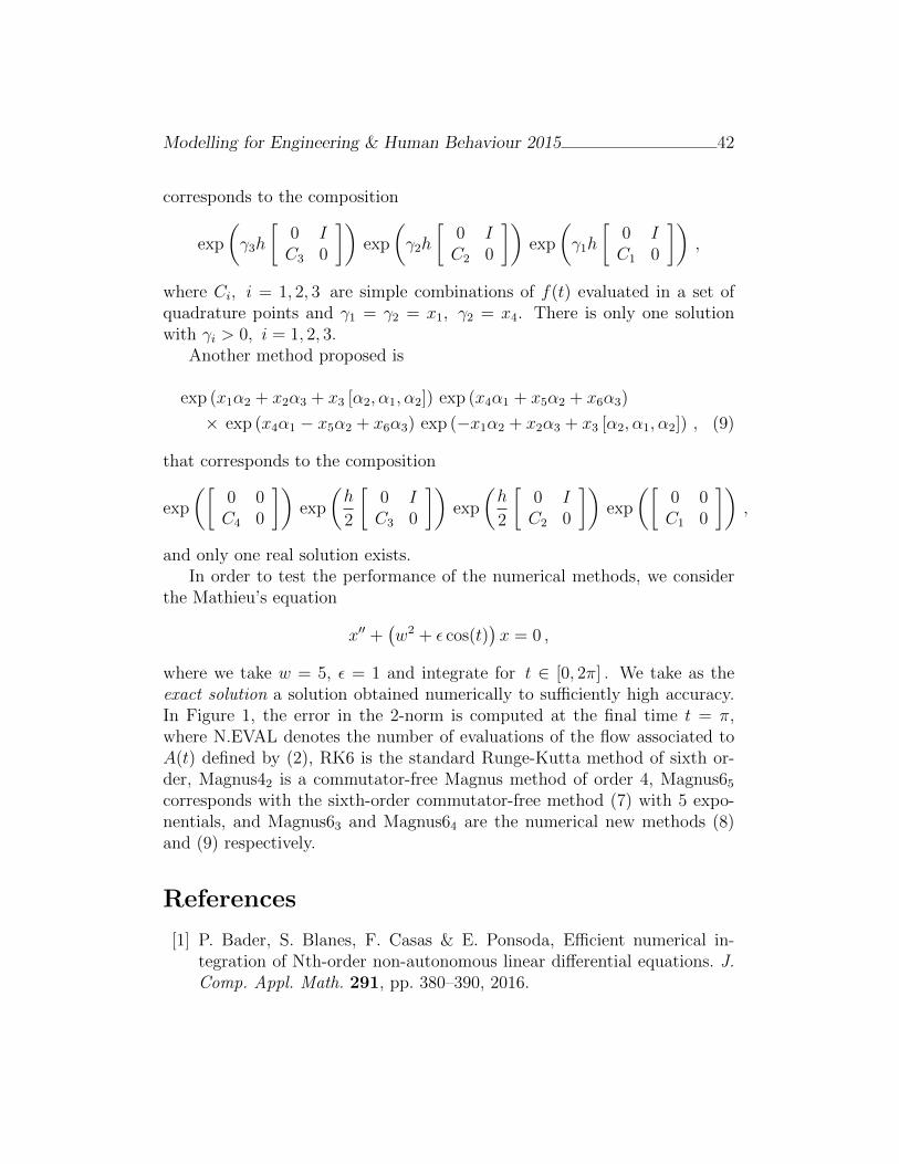
Modelling for Engineering & Human Behaviour 2015 42
corresponds to the composition
exp
(γ3h
[0 IC3 0
])exp
(γ2h
[0 IC2 0
])exp
(γ1h
[0 IC1 0
]),
where Ci, i = 1, 2, 3 are simple combinations of f(t) evaluated in a set ofquadrature points and γ1 = γ2 = x1, γ2 = x4. There is only one solutionwith γi > 0, i = 1, 2, 3.
Another method proposed is
exp (x1α2 + x2α3 + x3 [α2, α1, α2]) exp (x4α1 + x5α2 + x6α3)
× exp (x4α1 − x5α2 + x6α3) exp (−x1α2 + x2α3 + x3 [α2, α1, α2]) , (9)
that corresponds to the composition
exp
([0 0C4 0
])exp
(h
2
[0 IC3 0
])exp
(h
2
[0 IC2 0
])exp
([0 0C1 0
]),
and only one real solution exists.In order to test the performance of the numerical methods, we consider
the Mathieu’s equation
x′′ +(w2 + ε cos(t)
)x = 0 ,
where we take w = 5, ε = 1 and integrate for t ∈ [0, 2π] . We take as theexact solution a solution obtained numerically to sufficiently high accuracy.In Figure 1, the error in the 2-norm is computed at the final time t = π,where N.EVAL denotes the number of evaluations of the flow associated toA(t) defined by (2), RK6 is the standard Runge-Kutta method of sixth or-der, Magnus42 is a commutator-free Magnus method of order 4, Magnus65
corresponds with the sixth-order commutator-free method (7) with 5 expo-nentials, and Magnus63 and Magnus64 are the numerical new methods (8)and (9) respectively.
References
[1] P. Bader, S. Blanes, F. Casas & E. Ponsoda, Efficient numerical in-tegration of Nth-order non-autonomous linear differential equations. J.Comp. Appl. Math. 291, pp. 380–390, 2016.
Modelling for Engineering & Human Behaviour 2015 43
1.4 1.6 1.8 2 2.2 2.4
−10
−9
−8
−7
−6
−5
−4
−3
−2
−1
LOG(N.EVAL)
LOG(E
RROR)
Magnus42Magnus63Magnus65
RK6
Magnus64
Figure 1: Error at the final time t = π
[2] S. Blanes & P.C. Moan, Fourth- and sixth-order commutator-free Mag-nus integrators for linear and non-linear dynamical systems, Appl. Nu-mer. Math., 56, pp. 1519-1537, 2006.
[3] S. Blanes & E. Ponsoda, Time-averaging and exponential integratorsfor non-homogeneous linear IVPs and BVPs. Appl. Num. Math. 62, pp.875–894, 2012.
[4] R. Denk, On the Floquet exponents of Hill’s equation systems. Math.Nachr. 172, pp. 87–94, 1995.
[5] J. A. Richards, Analysis of periodically time-varying systems. Springer-Verlag. New York. 1983.
[6] L. Ruby, Applications of the Mathieu equation. Am. J. Phys. 64(1), pp.39–44, 1996.
[7] G. Teschl, Ordinary differential equations and dynamical systems. Grad-uate studies in mathematics, Vol. 140. AMS. U.S. 2012.
Adaptability of the acoustics of a room byvarying the height of the acoustic ceiling
P. J. Blazquez[ ∗and L. Orcos‡
([) Universidad Internacional de La Rioja (UNIR),
Av. Gran Vıa Rey Juan Carlos I, 41
26002, Logrono, La Rioja, Spain.
(‡) Universidad Nacional de Educacion a Distancia (UNED),
Calle Barriocepo, 34
26001 Logrono, La Rioja, Spain.
November 15, 2015
1 Introduction
Many problems from Applied Sciences including engineering can be solved bymeans of finding the solutions to equations using Mathematical Modelling [1,2]. For example, dynamic systems are mathematically modeled by differenceor differential equations, and their solutions usually represent the states ofthe systems.
Currently, several mathematical models for the analysis of reverberationtimes are used. Two of the most commonly applied models are the Sabine[3] and Eyring [4] as they can be used as methods for reverberation timescalculation [5, 6, 7, 8, 9] or as a comparative referencence for the applica-tion of new experimental methods [10, 11]. The application of these twomathematical models helps us to analyze and characterize the type of roomwith which we work, allowing us to estimate the behavior of reverberationtimes inside the room [5]. Both Sabine and Eyring Models, have served and
∗e-mail: [email protected]
44

Modelling for Engineering & Human Behaviour 2015 45
are still worth as a baseline in order to calculate the reverberation time indifferent types of enclosures, fact that makes them to be taken into accountas mathematical models in the study of the behavior of the halls [12].
The rest of the paper is organized as follows: in Section 2 we presentthe problem studied, in Section 3 two models are presented and in Section 4some tests and simulations are shown. Finally, the conclusions drawn to thisstudy are presented in the concluding Section 5.
2 Problem description
In this paper we analyze the application of the Sabine and Eyring mathe-matical models in three prototypes of acoustic rooms. We will observe if theresults obtained satisfy the desired conditions for the acoustic characteristicsof the different studied rooms. We will analyze the results of the reverber-ation times, by applying the Sabine and Eyring models, to prototypes ofacoustic rooms, which will be raised without any acoustic treatment. Theonly difference between these prototypes will be the variation in height ofcertain sections of the roof. What we want to show is that, by analyzing theresults obtained, when applying these two mathematical models to the pro-totypes raised, we can reach that the fact of installing a variable-conditioningceiling with acoustic materials, can let us have different rooms types in thesame one, being able to adapt the acoustic conditions, just varying the heightof the ceiling, optimizing the structural and acoustic characteristics of theroom.
3 Mathematical Models
Applying both mathematical models, we can calculate reverberation timesof our prototypes. These mathematical models help us to analyze and char-acterize the kind of room where we are, as we can estimate their behaviorthrough the results of reverberation times.
3.1 Sabine model
Sabine model is based on the existence of a diffuse field. The type of energyis specular, which fills the room with constant energy density, this meansthat the absorbent material is evenly distributed. To apply this model it has
Modelling for Engineering & Human Behaviour 2015 46
to be assumed that the average absorption coefficient is very low, less than0.3. Even so, this theory is applied to any asymmetrical distribution of theabsorbent material in a room and for any value of α [4].
The mathematical model attends to the following expression:
Rt =0.161× V
α× S
where
α =
∑n αn × Sn
Sso,
Rt =0.161× V∑n αn × Sn
being
• V = Room volume in cubic meters (m3).
• S = Total room surface (m2).
• α = Average absorption coefficient.
• Sn = Material absorption surface (m2).
• αn = Material absorption coefficient.
3.2 Eyring model
The Eyring model is based on the assumption of a diffuse field, that is tosay, it estimates that the absorption produced in the room is uniform. Thismodel is considered more accurate for average absorption coefficients greaterthan 0.3. When the value of the average absorption coefficient is very low,less than 0.3, the Eyring model tends to be the Sabine one [4].
The mathematical model attends to the following expression:
Rt =0.161× V
S× (ln(1− α))
where
α =
∑n αn × Sn
S

Modelling for Engineering & Human Behaviour 2015 47
so,
Rt =0.161× V
S× (ln(1−∑
n αn×Sn
S))
being
• V = Room volume in cubic meters (m3).
• S = Total room surface (m2).
• α = Average absorption coefficient.
• Sn = Material absorption surface (m2).
• αn = Material absorption coefficient.
4 Tests and simulations
In this section we will present the results of the application of the Sabineand Eyring models to the prototypes. These results will help us to analyzethe installation of a variable ceiling within a room.
In Figure 1 we show the results obtained in the simulation of prototypeswithout any acoustic treatment (7.0m Prototype, 7.05m Prototype 7.1m Pro-totype) letting us reflect on what it might mean the fact of changing theceiling of our prototype. To carry out this proposal, we will apply bothmathematical models, in order to analyze the reverberation times inside theprototypes. Then we will represent the results of reverberation times graph-ically and we will show the differences obtained in the two variations (from0 to 0.5 meters and from 0.5 meters to 1 meter) for the applied models.
5 Conclusions
We realize that the application of Sabine and Eyring mathematical modelsto this work acoustic Prototypes helps us to analyze their behavior as wevary the height of the sections of deployment of our roof.
Analyzing the results of the application of the mathematical models (seeFigure 1), we can see that the reduction of the reverberation time is consider-able. This fact indicates that the variation of the roof is a positive factor for
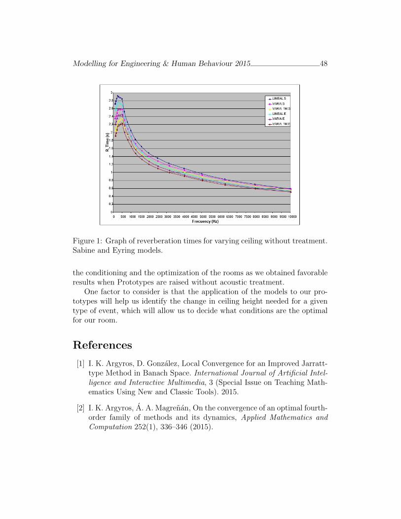
Modelling for Engineering & Human Behaviour 2015 48
Figure 1: Graph of reverberation times for varying ceiling without treatment.Sabine and Eyring models.
the conditioning and the optimization of the rooms as we obtained favorableresults when Prototypes are raised without acoustic treatment.
One factor to consider is that the application of the models to our pro-totypes will help us identify the change in ceiling height needed for a giventype of event, which will allow us to decide what conditions are the optimalfor our room.
References
[1] I. K. Argyros, D. Gonzalez, Local Convergence for an Improved Jarratt-type Method in Banach Space. International Journal of Artificial Intel-ligence and Interactive Multimedia, 3 (Special Issue on Teaching Math-ematics Using New and Classic Tools). 2015.
[2] I. K. Argyros, A. A. Magrenan, On the convergence of an optimal fourth-order family of methods and its dynamics, Applied Mathematics andComputation 252(1), 336–346 (2015).

Modelling for Engineering & Human Behaviour 2015 49
[3] W.C. Sabine, Dover Pub., 1900.
[4] C. F. Eyring, Reverberation time in dead rooms. Journal of the Acous-tical Society of America, 1930.
[5] N. Nishihara, T. Hidaka T, L. L. Beranek, Mechanism of sound absorp-tion by seated audience in halls. Journal of the Acoustical Society ofAmerica, 2001.
[6] H. Arau-Puchades, Improved Reverberation Formula. Revista deacustica, 1998.
[7] G. Moreira, A. Ramırez, Simulacion Computacional de Recintos Arqui-tectonicos y Modelos Matematicos V/S Condiciones Reales, CongresoInternacional de Acustica y Audio Profesional, 2011.
[8] J. Segura, R. Sanchis, J. Amarshi, E. A. Navarro, Condiciones acusticasde la camara anecoica electromagnetica de la Universitat de Valencia.Sociedad Espanola de Acustica, 2001.
[9] L. Leo, Analysis of Sabine and Eyring equations and their applicationto concert hall audience and chair absorption. Journal Acoustics, 2006.
[10] N. Bastian, R. Flores, Comparacion entre Modelacion del SoftwareEASE y Mediciones in situ. Sonac, 2012.
[11] C.E Boschi, A.F Gonzalez, Comparacion del valor teorico y la mediciondel TR60 mediante el metodo de la detonacion. EnIDI. Mendoza. Ar-gentina, 2008.
[12] H. Arau-Puchades, Revision del tiempo de reverberacion: El metodo decalculo, la precision y la ley. Congreso nacional de acustica, 2010.
Water pump scheduling Optimization using
Agent Swarm Optimization
B. Brentan‡ ∗, I. Montalvo†, E. Luvizotto Jr.‡ J. Izquierdo ⋆
and Rafael Perez-Garcıa⋆
()Computational Hydraulic Laboratory, University of Campinas,
Saturnino de Brito, 951, Campinas, Sao Paulo, Brazil,
(†) IngeniousWare GmbH,
Bahnhofstrae 4a, 76137, Karlsruhe, Germany,
(‡) Fluing - IMM, Universitat Politecnica de Valencia,
Camino de Vera, s/n, 5C bajo, Valencia, Spain.
November 30, 2015
1 Introduction
Utility companies must be able to supply water with the quality and quan-tity required by the consumers at the lowest energy consumption [?]. Tothis purpose, water supply management must be based on crucial decisionsabout maneuvers of pumps and valves, thus reducing energy consumptionand water losses. Optimized rules for water pumping, such as start andstop operations or speed variations bring better control of the system costs[?, ?]. Studies about pump operation, including both scheduling and rota-tion speed change decisions, have gained ground with the improvement ofcomputational resources and the development of hydraulic models able tosimulate the hydraulic behavior of water supply networks. And most re-cently, the application of optimization methods linked to such models hasachieved smarter and safer operational and strategic decisions [?].
∗e-mail: [email protected]
50
Modelling for Engineering & Human Behaviour 2015 51
However, to focus on engineering problem optimization operational con-straints to ensure the applicability of solutions in practice must be considered.One way to manage those constraints is by using multi-objective evolution-ary optimization considering contraints as additional objectives to be ful-filled. This idea has been applied to water supply systems for optimal designincluding reliability issues, sensor placement, calibration models and opera-tional rules. Considering a multi-objective approach and several constraintslinked to energy saving, we present an optimization based on Agent SwarmOptimization (ASO). Our solution takes into account not only pressure lim-its as constraints, but also limits on tank levels, water age, and the numberof pump maneuvers. As a result, applicable pump scheduling and efficientoperation of variable speed pumps are obtained.
2 Optimization Problem
The daily fluctuation of water demand and energy prices, the possibility ofmanaging tank levels, the operational limits on pressure, and the need tocontrol water quality improve the ability of the energy saving problem tomake decisions about pump status and speed. Keeping in mind the newparadigms for the cities, the main objective of finding optimal pump rules isthe reduction of energy consumption, which can be written according to
Min(Ce) =T∑
t=1
n∑
i=1
Qt,i ·Ht,i · γ
ηt,i, (1)
where Ce is the total cost, T is the total analysis time, usually 24 hours, Qt,i
is the flow at time step t for pump i, Ht,i is the head and ηt,i is the efficiencyof pump i at time step t.
To find the lowest cost means to find the best speed for each pump inthe system for each time step. So the decision vector v has componentsrepresenting the relative speed of each pump at each time step. The relativespeed showing the percentage of full speed is used. However, the use of lowspeed can bring operational problems and should be limited.
Pump operation is not only constrained by energy saving, but also bynormative and quality maintenance of distributed water parameters. Whilesingle objective algorithms treat constraints with penalty functions leavingdiscretionary the choice of multiplier parameters, multi-objective algorithms
Modelling for Engineering & Human Behaviour 2015 52
can treat constraints as objectives. In this way, objective functions are addedto the problem, corresponding to problem constraints.
So, the evaluation of the operational constraints is free of the empiricisminherent to the frequently arbitrary choice of penalty parameters. Howeverthe growing number of constraints requires of a robust algorithm to solvewith quality and agility the optimization problem. The following equationspresent the constraints we take into account in this work.
Min(Cp,min) =
Ntotal∑
node=1
(pmin − pnode,t), (2)
Min(Cp,max) =
Ntotal∑
node=1
(pmax − pnode,t), (3)
Min(Cm) =
n∑
i=1
mT,i −m⋆, (4)
Min(Cl) =
Ntanks∑
k=1
(lf,k − li,k), (5)
Min(Cw) =
Ntotal∑
node=1
(wnode − ws), (6)
where pmin is the minimal pressure required by the water system, pmax is themaximal pressure, pnode,t is the pressure at time step t at junction node, mT,i
is the number of start and stop operations at pump i, m⋆ is the maximalpump operation, Ntanks is the total number of tanks, lf,k and li,k are the finaland initial levels at tank k, wnode is the water age at a junction, and ws isthe standard water age required by the system to maintain quality.
3 Agent Swarm Optimzation - ASO
Agent Swarm Optimization (ASO) [?] is a generalization of Particle SwarmOptimization (PSO). The interaction among the agents enables the genera-tion of swarms, structures at an abstract viewpoint, which exhibit emergentbehaviors and interact with other agents. The algorithm increases the qual-ity of solutions because over the time the agents work in a distributed way
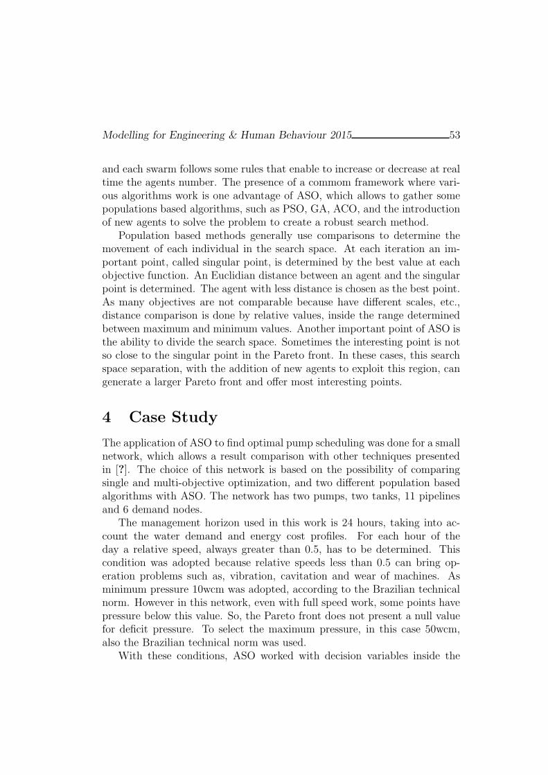
Modelling for Engineering & Human Behaviour 2015 53
and each swarm follows some rules that enable to increase or decrease at realtime the agents number. The presence of a commom framework where vari-ous algorithms work is one advantage of ASO, which allows to gather somepopulations based algorithms, such as PSO, GA, ACO, and the introductionof new agents to solve the problem to create a robust search method.
Population based methods generally use comparisons to determine themovement of each individual in the search space. At each iteration an im-portant point, called singular point, is determined by the best value at eachobjective function. An Euclidian distance between an agent and the singularpoint is determined. The agent with less distance is chosen as the best point.As many objectives are not comparable because have different scales, etc.,distance comparison is done by relative values, inside the range determinedbetween maximum and minimum values. Another important point of ASO isthe ability to divide the search space. Sometimes the interesting point is notso close to the singular point in the Pareto front. In these cases, this searchspace separation, with the addition of new agents to exploit this region, cangenerate a larger Pareto front and offer most interesting points.
4 Case Study
The application of ASO to find optimal pump scheduling was done for a smallnetwork, which allows a result comparison with other techniques presentedin [?]. The choice of this network is based on the possibility of comparingsingle and multi-objective optimization, and two different population basedalgorithms with ASO. The network has two pumps, two tanks, 11 pipelinesand 6 demand nodes.
The management horizon used in this work is 24 hours, taking into ac-count the water demand and energy cost profiles. For each hour of theday a relative speed, always greater than 0.5, has to be determined. Thiscondition was adopted because relative speeds less than 0.5 can bring op-eration problems such as, vibration, cavitation and wear of machines. Asminimum pressure 10wcm was adopted, according to the Brazilian technicalnorm. However in this network, even with full speed work, some points havepressure below this value. So, the Pareto front does not present a null valuefor deficit pressure. To select the maximum pressure, in this case 50wcm,also the Brazilian technical norm was used.
With these conditions, ASO worked with decision variables inside the
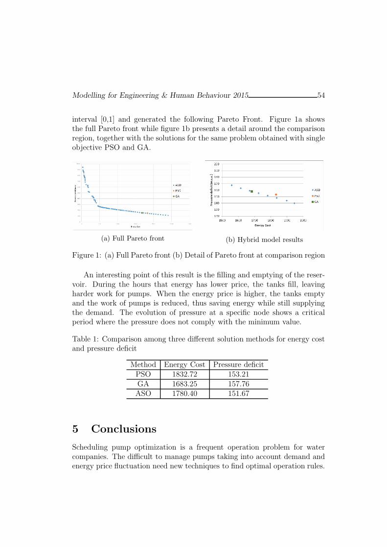
Modelling for Engineering & Human Behaviour 2015 54
interval [0,1] and generated the following Pareto Front. Figure 1a showsthe full Pareto front while figure 1b presents a detail around the comparisonregion, together with the solutions for the same problem obtained with singleobjective PSO and GA.
(a) Full Pareto front (b) Hybrid model results
Figure 1: (a) Full Pareto front (b) Detail of Pareto front at comparison region
An interesting point of this result is the filling and emptying of the reser-voir. During the hours that energy has lower price, the tanks fill, leavingharder work for pumps. When the energy price is higher, the tanks emptyand the work of pumps is reduced, thus saving energy while still supplyingthe demand. The evolution of pressure at a specific node shows a criticalperiod where the pressure does not comply with the minimum value.
Table 1: Comparison among three different solution methods for energy costand pressure deficit
Method Energy Cost Pressure deficitPSO 1832.72 153.21GA 1683.25 157.76ASO 1780.40 151.67
5 Conclusions
Scheduling pump optimization is a frequent operation problem for watercompanies. The difficult to manage pumps taking into account demand andenergy price fluctuation need new techniques to find optimal operation rules.

Modelling for Engineering & Human Behaviour 2015 55
This work presents an application of ASO, a multi objective optimizationalgorithm, thus eliminating the use of penalty functions. The Pareto frontcompared with previous GA and PSO results define an operational zonewhere the energy price decreases with a small increase of pressure deficit.
ASO is a generalization of PSO, treating swarms as agents and usingintelligent sel-adaptive parameters to find optimal values. The case studypresented here shows the efficiency of the method to build the Pareto front,reducing 25% of energy cost, while supplying demand and pressure nearbythe minimum values required.

Modelling for Engineering & Human Behaviour 2015_______________________________56
MATHEMATICAL MODELLING OF HEALTH
CARE EXPENDITURE ADJUSTED BY MORBIDITY
Vicent Caballer-Tarazonaª, Natividad Guadalajara-Olmedaª, David Vivas-Consueloª and Antonio
Clemente-Colladob
a) Research Centre for Health Economics and Management, Universitat Politècnica de
València, Cno de Vera s/n, Valencia, Spain
b) Denia Hospital. Marina Salud. Denia. Spain
1. Introduction
Econometric modelling of health care expenditure is a highly useful technique, among
other things for assigning capitation budgets, predicting health care use in the population
and improving planning and management of medical services. Traditionally, socio-
demographic variables (sex, income, social status) have been the most frequently used to
explain the factors that have an impact on health care expenditure. However, in recent years
various tools have appeared with the purpose of classifying the population into different
homogeneous groups of expenditure according to clinical risk (1,2).
To carry out this study, the system of patient classification we have used is CRG (3), the
system employed in the Valencia Community (Comunidad Valenciana) by the Directorate
of Pharmacy and Health Care Products (Dirección de Farmacia y Productos Sanitarios).
CRGs group population into 9 mutually exclusive health statuses according to diagnostics
from contacts with the health care system at all levels (pharmacy consumption, hospital
admissions, medical consultations, etc.). These health states are: 1) Healthy; 2) History of
significant acute disease; 3) Single minor chronic disease; 4) Minor chronic diseases; 5)
Single dominant chronic disease; 6) Chronic disease in 2 or more organ systems; 7)
Dominant chronic disease in 3 or more organ systems; 8) Dominant neoplasms, metastases
and complications; and 9) Extreme healthcare needs (Catastrophic conditions).
Within each health status, each patient may be further classified into 6 states of severity,
according to the extent of the clinical condition.

Modelling for Engineering & Human Behaviour 2015_______________________________57
However, to model health care expenditure we must bear in mind that there is positive
asymmetry in the distribution, with many registers equal to 0 and with a small proportion of
the public representing high cost, which causes heteroscedasticity when applying the
traditional OLS models(4). To compensate for these anomalies, Duan (5) proposes applying
a corrective coefficient, called a Smearing Estimator, to the lineal regression. Nevertheless,
other authors propose using Generalized Linear Models (GLM) as a more appropriate tool
to explain health expenditure (6). The GLM allow explanation of the result of an
endogenous variable when there is heteroscedasticity and the data distribution is not
normal.
The aim of this study is to model the total health care costs of patients from a single health
care district by applying different mathematical approaches.
2. Methodology
Data and Setting:
Data was collected for a total of 156,811 inhabitants from the Denia Health Department for
January to December 2013. The information concerning outpatient pharmaceutical
expenditure, primary health care contacts and CRG classification was extracted using the
corporate systems of the Valencia Community Regional Health Ministry (Conselleria de
Sanidad de la Comunidad Valenciana): SIP, SIA, CRC and GAIA.
Variables:
A database indicating the cost per patient was designed, which included pharmaceutical and
medical expenditure in the Denia Health Department. Each patient was placed in their
corresponding CRG according to their morbidity.
Modelling:
Both the multivariate linear regression logarithmic (MLR) and the generalized linear model
(GLM) were applied with health expenditure being the dependent variable and CRG health
status and demographic variables (age and sex) as the independent variables.

Modelling for Engineering & Human Behaviour 2015_______________________________58
Various modellings were carried out which included demographic and morbidity variables
and those with the greatest level of explanation according to the coefficient of
determination were chosen.
In both methodologies the logarithmic transformation of the dependent variable was carried
out to increase the goodness of fit and avoid problems of heteroscedasticity.
The log regression model takes the form:
LnY= Lnβ0 + Lnβ1*x1 + Lnβi*xi+εi (1)
Where:
• LnY= Naperian logarithm of Health Expenditure
• LnΒi =Parameter measuring the incidence of Group i on dependent variable in
logarithmic terms.
• Xi= Each of the clinical risk groups and severity level.
• εi = Smearing Estimator
Values and a severity level are obtained for each group through the regression coefficients.
Next, the logarithm of each group of patients is undone applying the exponential, after
which it is multiplied by the Smearing Estimator (mean of the exponential of the regression
residuals). Lastly, 1 is subtracted from the resulting value, as prior to carrying out the
regression 1 was added to all cost values to avoid the loss of data equal to 0 in the
logarithmic transformation.
The GLM Model takes the form
ηi = β0 + β1x1i + ... + βpxpi (2)
Where:
• LnY= Health Expenditure
• LnΒi =Parameter measuring the incidence of Group i on dependent variable
• Xi= Each of the clinical risk groups and severity levels and two functions
• a link function that describes how the mean, E(Yi) = µi , depends on the linear
predictor

Modelling for Engineering & Human Behaviour 2015_______________________________59
g(µi) = ηi I
• a variance function that describes how the variance, var(Yi) depends on the mean
var(Yi) = φV (µ)
where the dispersion parameter φ is a constant.
The value of the coefficient was transformed, undoing the logarithm to calculate the
predicted values for the model.
Goodness of fit for both models was compared estimating the correlation coefficient
between the real and predicted values for both models.
3. Results:
The total health care expenditure on the patients covered by the Denia health department
(156,811 people) in 2013 was 154,114,807.85 Euros. 18.96% of the population had no
contact with the health system, and therefore had zero cost. 76.93% had a cost less than the
mean, of which 43.55% registered a cost of less than 100 Euros.
On the other hand, on classifying the department population into the 9 CRG health statuses
it was observed that 54.63% of the population was classified as healthy, with a
consumption representing 13.34% of the total. The health statuses with the greatest burden
on the health system are those of group 5, single dominant or moderate chronic disease, and
group 6, significant chronic disease in multiple organ systems. Group 6 supposes 33.36%
of total department expenditure for a population that encompasses only 10.02% of the total.
Patients in group 5 incurred 25.87% of the total expenditure, while being 15.85% of the
population. The total consumption of health care resources for these two groups was
58.23%, while their demographic weight of 25.86% of the population is relatively small for
their volume of expenditure.

Modelling for Engineering & Human Behaviour 2015_______________________________60
Table 1. Percentage of population and expenditure according to CRG health status and severity level.
Severity levels, obviously, also affect health expenditure considerably, as appreciated in
Table 1.
The results of the OLS models are presented in Table 2. The model with the greatest
coefficient of determination was number 5, which combined the CRG health statuses, age
and sex. Nevertheless, to develop a more practical management tool, we chose model 3,
which only includes the CRG health status and severity level, but has a more simple
implementation, although a slightly inferior coefficient of determination than model 5.

Modelling for Engineering & Human Behaviour 2015_______________________________61
Table 2. Linear Regression Coefficients
In the same way the coefficients for the various models were calculated through the GLM
Table 3.
Model 1 Model 2 Model 3 Model 4 Model 5
Age rangeCRG Health
Status
CRG Health
Status, and
Severity level
CRG Health
Status,age &
sex
CRG Health
Status,severity
level, age and sex
Constant 4.124 4.124 3.38 3.74 3.76
Age -0.02 -0.02
Sex (Female) 0.32 0.32
Age 0-1 1.749
Age 2-14 0.481
Age 15-24 -0.082
Age 25-34 -0.04
Age 45-54 0.486
Age 55-64 1.166
Age 65-74 1.664
Age 75-84 2.421
Age 85 + 2.628
Health Status 2 2.824 2.82 2.84 2.84
Health Status 3 2.369 2.34 2.54 2.52
Health Status 4 3.199 2.95 3.50 3.25
Health Status 5 3.288 3.12 3.61 3.44
Health Status 6 4.22 3.88 4.74 4.39
Health Status 7 4.906 4.36 5.56 4.98
Health Status 8 4.991 4.39 5.45 4.81
Health Status 9 5.631 5.01 5.95 5.28
Severity level 2 0.54 0.58
Severity level 3 0.76 0.84
Severity level 4 0.96 1.09
Severity level 5 1.14 1.31
Severity level 6 1.57 1.67
F 1836.893 12966.873 8141.80 11044.67 7544.34
R2 0.095 0.398 0.403 0.413 0.419
Variables

Modelling for Engineering & Human Behaviour 2015_______________________________62
Table 3. Generalised Linear Models
Model 1 Model 2 Model 3 Model 4 Model 5
Age rangeCRG Health
Status
CRG Health
Status and
Severity level
CRG Health
Status,age &
sex
CRG Health
Status,severity
level, age and sex
Constant 7.854 5.485 5.485 5.543 5.547
Age -0.005 -0.006
Sex (Female) 0.201 0.206
Age 0-1 -0.726
Age 2-14 -0.926
Age 15-24 1.236
Age 25-34 3.347
Age 35-44 4.251
Age 45-54 3.300
Age 55-64 1.923
Age 65-74 1.018
Age 75-84 0.322
Age 85 + 0.000
Health Status 2 1.437 1.437 1.453 1.454
Health Status 3 1.039 0.997 1.129 1.093
Health Status 4 1.549 1.320 1.678 1.453
Health Status 5 1.896 1.728 2.058 1.891
Health Status 6 2.579 2.249 2.801 2.467
Health Status 7 3.158 2.665 3.433 2.936
Health Status 8 3.701 3.203 3.902 3.399
Health Status 9 4.092 3.446 4.297 3.633
Severity level 2 0.432 0.429
Severity level 3 0.634 0.650
Severity level 4 0.850 0.879
Severity level 5 0.947 1.002
Severity level 6 1.492 1.491
Deviance 1266380.53 451444.74 447127.05 443531.69 443531.69
Deviance climbing 1266380.53 451444.74 202345.12 202122.06 202122.06
Pearson Chi-square 189988.55 1180231.57 1144768.90 1178770.93 1178770.93
Pearson chi-square scaling 189988.55 1180231.57 518059.47 537178.32 537178.32
Maximum likelihood -1555099.04 -1147631.14 -1098785.81 -1097969.44 -1097969.44
Akaike information criterion (AIC) 3110218.08 2295280.29 2197601.62 2195972.88 2195972.88
Finite sample corrected AIC (AICC) 3110218.08 2295280.29 2197601.62 2195972.88 2195972.88
Bayesian Information Criterion (BIC) 3110317.71 2295369.95 2197751.06 2196142.25 2196142.25
Consistent AIC (CAIC) 3110327.71 2295378.95 2197766.06 2196159.25 2196159.25
Variables

Modelling for Engineering & Human Behaviour 2015_______________________________63
After carrying out the linear regression relating the value estimated by the models and the
real value, the coefficient of determination was calculated (Table 4). The proposed values
for the GLM present the best R2 of the three methodologies.
Table 4. Coefficient of determination for the linear regression between real and estimated value.
LM GLM Adjusted Patients CRG
Squared
correlation 0.247 0.255 0.214
4. Conclusion
By means of the CRG, it is possible to establish a Case Mix system appropriate for defining homogeneous consumption patterns, thus improving the efficiency of health care organizations. Furthermore, this Case Mix system may be useful to predict the allocation of health care resources for the population according to their CRG health status.
5. References
1. Ellis RP, Pope GC, Iezzoni L, Ayanian JZ, Bates DW, Burstin H, et al. Diagnosis-based
risk adjustment for Medicare capitation payments. Health Care Financ Rev.
1996;17(3):101–28.
2. Starfield B, Weiner J, Mumford L, Steinwachs D. Ambulatory care groups: a
categorization of diagnoses for research and management. Health Serv Res.
1991;26(1):53–74.
3. Hughes JS, MD; Averill RF, MS; Eisenhandler J, PhD; Goldfield NI, MD; Muldoon,
John MHA; Neff, John M. MD§; Gay JCM. Clinical Risk Groups (CRGs): A
Classification System for Risk-Adjusted Capitation-Based Payment and Health Care
Management. Med Care. 2004;42(1):81–90.

Modelling for Engineering & Human Behaviour 2015_______________________________64
4. Jones AM. Models for health care. 2010;(January). Available from:
http://www.york.ac.uk/media/economics/documents/herc/wp/10_01.pdf
5. Duan N. Smearing estimate - a nonparametric retransformation method. J Am Stat
Assoc. 1983;78(383):605–10.
6. Hill E, Miller E. Health expenditure estimation and functional form: applications of
the generalized gamma and extended estimating equations models. Health
Econ. 2010 May;19(5):608-27

Modelling for Engineering & Human Behaviour 2015_________________________65
CALCULATED FORECAST FOR TECHNICAL
OBSOLESCENCE IN COMPUTERISED
TOMOGRAPHY EQUIPMENT.
Francisco Reyes-Santiaª, Vicent Caballer-Tarazonab, Fernándo Gómez-López
c, Javier
Rivero de Aguilar-Ameneiroc and David Vivas-Consuelo
b
a) Facultad de Ciencias Empresariales y Turismo. Universidad de Vigo. Spain
b) Research Centre for Health Economics and Management, Universitat Politècnica de
València, Caminoo de Vera s/n, Valencia, Spain
c) FIS-Instituto de Salud Carlos III. Madrid. Spain
1. Introduction
To estimate the useful life of Computerised Tomography Equipment (CT), with the aim
of planning a budget the purchase of equipment and for the renewal of CT equipment
within an already installed base so as to, therefore, maintain and ensure quality in
providing an imaging diagnostic level in the National Health System.
Technical obsolescence is an increasingly decisive factor in the development and
maintenance of all kind of health care equipment, particularly in medical imaging [1]
The design of a prediction model provides an advance warning of the appearance of any
technology leap that involves technological obsolescence in Computerised Tomography
technology in use.
The starting data is made up by the different Computerised Tomography models
commercialised since 1974 and that have provided a technology leap in CT technology.
It is necessary to know if the data distribution fits into a normal curve, because if this is
not so the data will be transformed. A main components analysis in this methodology
has allowed for a reduction in the number of variables on the survey-file in
Computerised Tomography technology and facilitates subsequent work without a
significant loss of information. The Log Binomial Regression Model has enabled
probability calculations on answers (technology leap) to the different levels of stimuli
(changes in variables, temporary development, detection system, imaging resolution and
equipment power). Using a Discriminant analysis, the objective has been to estimate,
based on time, the chances of a technological leap occurring [2] [3].

Modelling for Engineering & Human Behaviour 2015_________________________66
2. Methodology
To estimate the technological life of Computerised Tomography equipment (CT) with
the aim of planning a purchasing budget to obtain equipment and renew the already
installed base of technology equipment (CT) and therefore maintain and ensure quality
in providing an imaging diagnostic level in the National Health System.
The design of a prediction model provides an advance warning of the appearance of any
technology leap that involves technological obsolescence in Computerised Tomography
Technology in use.
3. Results:
Main Components Analysis
The strategy followed has been to find a solution that enables us to explain the
maximum percentage of variance and an acceptable parsimony of the model and to
reduce the 18 descriptive CAT model variables; to set the explained percentage of
variance in 92.9%, which is fulfilled in the first six factors in the present study and
represented in graphic 1.
Graphic 1
A rotation of factors has been done and the varimax orthogonal rotation method has
been used (axis turn orthogonally, in the same angle), which is intended to minimise the
number of variables with high saturations in the same factor. The aim of this method is
to increase the highest saturations in a factor, while decreasing the lowest for the factor
to be easily interpretable.
1 2 3 4 5 6 7 8 9 10 11 12 13 14 15 16 17 18
Component Number
0
2
4
6
8
10
12
14
Eig
en
valu
e
Scree Plot

Modelling for Engineering & Human Behaviour 2015_________________________67
The importance of each factor is evaluated considering the proportion of variance
explained by the factor after rotation.
The 18 evaluated technical parameters in Computerised Tomography Technology have
been grouped in three main components: Detection System (detector material,
reconstruction matrices, reconstruction time, chest and abdomen scans, CT number
range (HU), Processor, Maximum tube power (kW), scans ways) which explains 72.4%
of the variance; Imaging Resolution (cutting thickness range, hard disk, selected kV,
fine beam, thick beam) which explains 13.55% of the variance and Equipment Power
(X-ray generator, number of data by turn or image, digital subtraction) which explains
7.1% of the variance.
Analysis Logit
The characteristics shown by the design of a provision model in a technology leap
demands the econometric specification is carried out through carefully chosen models,
the endogenous variable to model is a categorical variable with various response
alternatives. Within this modelling typology, Logit methodology adjusts to this aim
using logistics as an adjusting function. The use of this function ensures that the
estimation result can be interpreted as the occurrence probability of each endogenous
variable alternative because the estimated values are always between the variation range
0-1.
Within the Logit modelling models of dichotomous answer and multiple answer models
are distinguished, according to whether the endogenous variable to model has two or
more answer alternatives with different specification in both cases. For a single case of
dichotomous variable, in which there are only two possible answer alternatives (there is
a technology leap or not), the endogenous variable is usually coded with 1 to represent
the occurrence of the studied event or 0 to represent the non-occurrence.
The explanatory variables used in the model are the 3 main components previously
calculated. The prediction model obtains a successful percentage of 76.9%. Table 2
presents the results of the Logit model for the current research, showing its estimated
coefficient β for the equation variables, typical error of β (S.T.), the Wald statistic, the
degrees of freedom (df) and the p-value for the significance of the estimated coefficient
(Sig.), the reason for the estimated advantages (Exp(β)) and the confidence interval for
exp(β) at 95%.
Table 1.
VARIABLES β Std. Error Wald df Sig. Exp(B)
Intercept -6,717 3,249 4,275 1 0,039
DETECTION -3,975 1,901 4,372 1 0,037 0,019
RESOLUTION -3,766 1,814 4,312 1 0,038 0,023
POWER -2,461 0,998 6,076 1 0,014 0,085
YEARS 0,431 0,194 4,904 1 0,027 1,538
The logistic regression allows us to approximate an assessment on the influence of each
main component with the passing of time, the implementation of a technology leap,

Modelling for Engineering & Human Behaviour 2015_________________________68
with its significant influence with positive signs of temporary evolution (0.430), and
with a negative sign for the main component the detection system(-3.974), image
resolution (-3.766) and equipment power (-2.460), as well as a technology leap
expectative depending on the independent variables influence for temporary evolution
(1.538) and main components, detection system (0.018) image resolution (0.023) and
equipment power (0.085).
Discriminant Analysis
The monitoring periods of this type of analysis are almost always different given that
the CT models incorporate into the study at different periods of the observation, in
which case, the last in doing so have been observed during a lesser period than those
that entered at the beginning. The failure time of each model is measured from the start
date of each model’s study. Every model has real time, this corresponds to its
incorporation date until its last observation and a time “t” which represents time (in
years, months, days and so on), the time in which each model was monitored.
The Discriminant methodology has been used so that the intervals are determined by the
event occurrence, that is to say, the survival probability is calculated every time an
event happens. The conditional probability of survival, this being the probability of
being a survivor at the end of an interval which is conditioned by the fact that each
model is already a survivor at the start of the interval, is calculated from the exact
number of risk cases when the event occurs. This assumes that the instantaneous rate is
zero during the interval between two events.
The Discriminant analysis can be used to estimate the probability of changing the CT
model over a determined period of time and the factors influencing.
As in the Log Binomial, the explanatory variables used in the model are the 3
components calculated. The prediction model obtains a lower percentage of success
than the Log Binomial, around 66.7%.
Table 2 presents the results of the Discriminant analysis, showing the estimated
coefficient for the equation variables. The Canonical correlation shows a result of 0.481,
meaning a good discrimination for the function. Moreover, the Lambda Wilkx shows a
value of 0.769 and a p-value of 0.05.
Table 2.
Variables Coefficients
DETECTION 1,822
RESOLUTION 2,250
POWER 1,147
YEARS -2,888
The most important factor in influencing the change of technology seems to be the
image resolution followed by the detection system and a negative sing for temporary
evolution.

Modelling for Engineering & Human Behaviour 2015_________________________69
4. Conclusion Remarks
The results of the present project will enable advance knowledge of the expectations of
technological change in CT technology, allowing an advance in investment planning for
this technology, for acquiring and installing the equipment in hospitals where this type
of technology still does not exist and for the renewal of technology bases already
installed.
The results of the present research can be validated by the application of other medical
technologies, thus amplifying the impact of this research.
All this will have to be reflected by an investment budget plan for technology
acquisition.

Modelling for Engineering & Human Behaviour 2015_________________________70
References
[1] E. Society, “Renewal of radiological equipment.,” Insights Imaging, vol. 5, no. 5,
pp. 543–6, 2014.
[2] P. Sandborn, “Forecasting Technology and Part Obsolescence,” no. November,
pp. 1–13, 2010.
[3] N. Joshi, F. Stahnisch, and T. Noseworthy, Reassessment of Health
Technologies: obsolescence and waste, no. December. 2009.
Heuristic Framework to Jointly CalibrateLeakage and Pressure in Water Distribution
Systems
E. Campbell‡ ∗, B. Brentan†, J. Izquierdo ?
and Rafael Perez-Garcıa?
(‡) Berliner Wasserbetriebe, Anstalt des ffentlichen Rechts
10864 Berlin, Amtsgericht Charlottenburg, HRA 30951 B, Germany
(†) Computational Hydraulic Laboratory, University of Campinas,
Saturnino de Brito, 951, Campinas, Sao Paulo, Brazil,
(?) Fluing - IMM, Universitat Politecnica de Valencia,
Camino de Vera, s/n, 5C bajo, Valencia, Spain.
November 30, 2015
1 Introduction
Usually, calibration of water distribution systems (WDSs) is performed byjust changing pipe roughness values and water losses are not usually con-sidered. Furthermore, a point highlighted by [4] is pipe grouping, which canbring several errors in calibration processes if flow distribution is not suitablybalanced within the groups.
A common way to add water losses in a calibration problem is to asso-ciate nodes with emitter coefficients through flow balances. First, a globalcoefficient responsible to comply with daily demand balance is found. Then,a multiplier of hourly water demand is changed interactively to find somehourly flow balance. However, considering the physical correlation of water
∗e-mail: [email protected]
71
Modelling for Engineering & Human Behaviour 2015 72
losses and pressure this approach can bring some errors. If losses are fixedand pipeline roughness is changed, pressure change and flow balance may fail.Also, if roughness is fixed first, the emitter coefficients are fully conditionedby this distribution. All in all, it is obvious that a joint adjustment of pipelineroughness and node emitter coefficients is a more appropriate approach.
Taking into account optimization features of the calibration problem, sev-eral methods have been proposed for fast and accurate solution, such as linearand non-linear methods, and recently, bio-inspired algorithms. Among themost known bio-inspired methods, Genetic Algorithms (GAs) have been ap-plied to solve various optimization problems in WDSs.
Bearing in mind the difficulty to calibrate roughness and emitter coef-ficients, we propose a joint calibration of these parameters using GAs foroptimization applied to an objective function designed by its features andability to facility GA convergence. Clustering methods and self-organizedmaps for grouping pipes and nodes are used as a way to reduce the dimen-sion of the problem.
2 Optimization problem
2.1 Problem definition
Calibration of WDSs may be regarded as a minimization of the error betweenmeasured and simulated hydraulic parameters, subject to nodal pressure andpipeline flow contraints. In this work, we consider group roughness values,demand pattern factors, and emitter group coefficients as decision variables.
To obtain an accurate model, a right decision must be made on the ob-jective function, even when the problem is solved by bio-inspired algorithms.The absolute error and the relative absolute error, [5], are applied in severalworks as objective functions. Also the square error is widely applied, and [2]uses this function to monitor nodal pressure.
However, the sole use of pressure as the monitored variable is not alwaysable to bring the required accuracy for the model, and pipeline flows have tobe considered to reduce uncertainty and improve the results. In this way, asum of absolute pressure, flow and tank level errors is proposed by [3]. Sincethis approach takes into account more than one hydraulic parameter, thedifferences among variable scales can lead to convergence problems.
Considering the difficult of obtaining a good objective function able to
Modelling for Engineering & Human Behaviour 2015 73
describe correctly the problem and to be solved without too many conver-gence problems we test a set of objective functions to compare not only themodel final accuracy, but also the computational effort needed to find thesought results. To evaluate those functions we use hypothesis tests based onthe assumption that the mean value of measured and simulated values donot diverge significantly. If this hypothesis is not validated, the respectiveobjective function will not be accepted.
Our statistical hypothesis test shows that an objective function can beaccepted, if none of the tested mean values (in our case, six pressure valuesand one flow value) shows a probability value lower than certain threshold.Also the coefficient correlation (r2) among measured and simulated values isused to compare the model accuracy. However all the considered functionspresented a high value of this parameter, close to 1, corresponding to highability of finding good results.
Still, an important factor in bio-inspired optimization is the convergencetime. The search can be hampered by local minima which may slow thesearch. These local minima are closely linked to the objective function.Therefore, we propose a quality index (QI) to evaluate not only the ac-curacy of the model, but also the computational effort. For an objectivefunction o, QI is defined by
QIo =
E∏e=1
r2e
iteromin(Iter)
, (1)
where r2e is the correlation coefficient for control element e in the studiednetwork, having E control elements, itero is the total iteration required tostop the optimization method using objective function o, and Iter is a vectorwith the number of iterations for each objective function.
The best value for parameter QI is found by composing dimensionlessabsolute errors using maximum and minimum flow and pressure:
Minf(Q,H) =
p∑k=1
|Qk −Qmk
Max(Q)|+
N∑n=1
| pn − pknMax(p)
| (2)
Minf(Q,H) =
p∑k=1
|Qk −Qmk
Min(Qk)|+
N∑n=1
| pn − pknMin(pk)
| (3)
Modelling for Engineering & Human Behaviour 2015 74
where Qk is the simulated flow through pipe k, Qmk is the modeled flow for
the same pipe, Q is a vector containing all measured flows, pn is the pressureat node n, pmn is the pressure modeled at the same node, and p is a vectorcontaining all measured pressures.
Regarding the optimization algorithm, this work uses a version of GAdeveloped by Palisade linked with MS Excel, using the demand pattern fac-tor, the number of pipeline groups, and the number of node groups as thelength of the decision vector. An iterative process of hydraulic simulationsand optimization algorithm runs is done, which evaluates the error for 60chromosomes.
3 Node and pipeline clustering
Keeping in mind the importance of the correct choice of the objective func-tion, another fundamental process involved with the calibration problem isthe correct grouping of pipelines and nodes, especially for large WDSs. Thevariation of roughness coefficients and water losses depend on a set of vari-ables. We claim that the use of clustering methods can help divide theelements into homogeneous groups. A cluster is defined as a conglomerate ofobjects that has similar features.
3.1 Self organized maps - SOMs
SOMs are a type of unsupervised neural networks, with unconnected nodesthat are fully connected to the input. Frequently, SOMs are used to repre-sent multidimensional databases through a two-dimensional structure. ThusSOMs can be used as a clustering a technique.
The first step to build a SOM is to define its topology. This meansto define the number of neurons (models), which depend on the implicitstructure of the database. Usually this structure is not known and the testof several topologies can help define the size of the map. The main idea is tofind an uniform distribution of the database multidimensional vectors amongthe neurons. To this purpose a distance among the elements is used as anindicator of similarity. The smaller the distance among elements associatedto the same neuron, the better the topology [1].
Once defined the topology of a SOM, it is important to define some train-ing parameters. Parameters help associate each neuron with an artificial
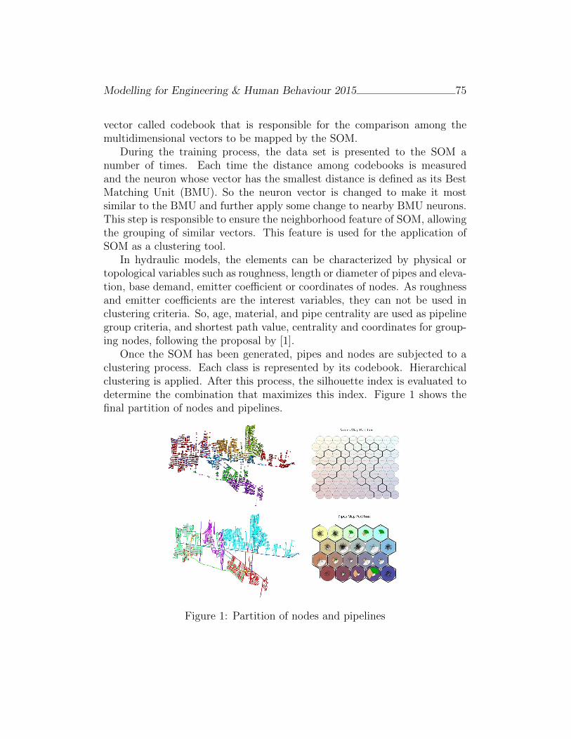
Modelling for Engineering & Human Behaviour 2015 75
vector called codebook that is responsible for the comparison among themultidimensional vectors to be mapped by the SOM.
During the training process, the data set is presented to the SOM anumber of times. Each time the distance among codebooks is measuredand the neuron whose vector has the smallest distance is defined as its BestMatching Unit (BMU). So the neuron vector is changed to make it mostsimilar to the BMU and further apply some change to nearby BMU neurons.This step is responsible to ensure the neighborhood feature of SOM, allowingthe grouping of similar vectors. This feature is used for the application ofSOM as a clustering tool.
In hydraulic models, the elements can be characterized by physical ortopological variables such as roughness, length or diameter of pipes and eleva-tion, base demand, emitter coefficient or coordinates of nodes. As roughnessand emitter coefficients are the interest variables, they can not be used inclustering criteria. So, age, material, and pipe centrality are used as pipelinegroup criteria, and shortest path value, centrality and coordinates for group-ing nodes, following the proposal by [1].
Once the SOM has been generated, pipes and nodes are subjected to aclustering process. Each class is represented by its codebook. Hierarchicalclustering is applied. After this process, the silhouette index is evaluated todetermine the combination that maximizes this index. Figure 1 shows thefinal partition of nodes and pipelines.
Figure 1: Partition of nodes and pipelines
Modelling for Engineering & Human Behaviour 2015 76
4 Conclusions
The calibration of a WDS model that considers not only roughness but alsoleaks through emitter coefficients, and hourly demand factors is not easy andrequires suitable optimization to define right values. The errors and difficul-ties of the process derive not only from adequate grouping processes but alsofrom suitability of the objective function that will describe the problem. Wepresent an approach, to jointly calibrate these three parameters using a bio-inspired genetic algorithm. To define the decision variables, we applied selforganizing maps that adequately divide pipelines and nodes into groups. Anobjective function using absolute error weighting of maximal and minimalvalues of control parameters (flow and pressure) is used, once the qualityindex of this function is the best.
This methodology presents computational time saving, finding high cor-relation parameters between measured and simulated variables, and reducingthe number of variables, once an SOM is able to define representative groups.
References
[1] E. Campbell, J. Izquierdo, I. Montalvo, A. Ilaya-Ayza, R. Perez-Garcıa,and M. Tavera. A flexible methodology to sectorize water supply net-works based on social network theory concepts and multi-objective opti-mization. 2015.
[2] T. Koppel and A. Vassiljev. Calibration of a model of an operationalwater distribution system containing pipes of different age. Advances inEngineering Software, 40(8):659–664, 2009.
[3] K. Lansey, W. El-Shorbagy, I. Ahmed, J. Araujo, and C. Haan. Cali-bration assessment and data collection for water distribution networks.Journal of Hydraulic Engineering, 127(4):270–279, 2001.
[4] R. W. Meier and B. D. Barkdoll. Sampling design for network model cal-ibration using genetic algorithms. Journal of Water Resources Planningand Management, 126(4):245–250, 2000.
[5] L. E. Ormsbee. Implicit network calibration. Journal of Water ResourcesPlanning and Management, 115(2):243–257, 1989.
A novel framework to sectorize water supplynetworks considering uncertainties
Enrique Campbell[ ∗, Joaquın Izquierdo†, Rafael Perez-Garcıa†,and Idel Motalvo‡
([) Berliner Wasserbetriebe
Neue Judenstraße 1, 10179, Berlin, Deutschland.
(†) Universitat Politecnica de Valencia
Camino de Vera SN, 46022, Valencia, Espana.
(‡) IngeniousWare GmbH
Bahnhofstraße 4a, 76137, Karlsruhe, Deutschland.
November 30, 2015
1 Introduction
Water Supply Network (WSN) sectorization entails the partial isolation ofareas within the networks by closing pipes and setting a flowmeter in a single(or few) feed lines. It has some drawbacks, namely, the economic investmentin boundary valves and flowmeters and the pressure reduction due to increaseof headloss. Whilst pressure reduction can translate into leakage reduction, itcan also lead to supply outage. A good sectorization layout must offset theseaspects; therefore, an optimal distribution of boundary valves and flowmetersmust be defined. In the methodology here proposed, the network is treatedas a social network, and a community detection algorithm is implementedto define the sectors, then, the arrangement entrances/boundaries is definedfor each sector using Genetic algorithms (GA) + Monte Carlo Simulation(MCS).
∗e-mail: [email protected]
77
Modelling for Engineering & Human Behaviour 2015 78
2 Community detection algorithm
WSNs can be represented as graphs, which allows to implement algorithmsderived from the graph theory domain. In the method proposed by Campbellet al. (2015) to define the trunk network, pipes are ranked according to theirrole in the supply of the entire network. For each node, the Shortest Paths,to all reachable nodes are calculated. The result is arranged in a square ma-trix, from where the Accumulated Shortest Path Value (ASPV) of each nodeis calculated and then, the values are transferred to pipes. This way, pipesconnected to the sources are expected to have the greatest values of ASPV,whilst the extreme pipes are expected to have an ASPV equals 1. This isused as a criterion to segregate the trunk network from the distribution net-work. The resulting distribution network is treated as a Social Network,and the Multilevel Community Detection Algorithm (Blondel et al., 2008)is implemented over it. The partition of the network with the highest valueof Modularity (Newman, 2006) index can generate extremely small commu-nities. Therefore, the communities in this partition are recursively mergedusing a merging process here proposed (see pseudocode below), to ensurethat all sectors comply with a series of pre-established limits. Such limitscan include, pipe length, number of connections, or a combination of severalcharacteristics.
Pseudocode:All pipes connecting communities are selected and put in a Set of Candidate Pipes(SCP); (1) Given pipe m, if INm ∈ Ci & FNm ∈ Cj −→ m ∈ SCP; from the CP,extract the subgroup of pipes scpi from which their corresponding communitiesdo not exceed a pre-established limit for a given feature; (2) Given scpi ∈ SCP,where, for every m, Li & Lj < Lmax; for every m, if Li + Lj < Lmax −→ i + j =i ∩ j; Steps 1-2 are repeated until no new pipes enter the scpi.
Here m = pipe; INm = initial node of pipe m; FNm = final node of pipe m;C = community; L = the characteristic used as a criterion.
Finally, the trunk network is re-coupled with the distribution network and thepipes connecting each sector with the first one are included among the SCP. Eachpipe inside the mentioned set can be defined either as boundary valve or as sectorentrance.
Modelling for Engineering & Human Behaviour 2015 79
3 Entrance-Closing valves definition
Between the unavoidable leakage volume and the total leakage volume that can befound in a typical WSN, there is an economic management level, which correspondsto the level where the cost of a new repair exceeds the benefits from the savings.One way to estimate such economical leakage level is through the assessment ofthe SRELL (Short Run Economic Leakage Level) based on a combination of theBABE (Background and Burst Estimates) concept (Thornton et al., 2008), andthe FAVAD (Fixed and Variable Area Discharge) theory (May, 1994). A very im-portant result derived from this estimation is the URELL (Lambert and Lalonde,2005), which corresponds to the volume of unreported leaks that is feasible to letoccur within one year. The method to estimate the SRELL includes an equation tocalculate the Optimal Frequency of Inspection (OFI) of the WSN, which is basedon three components: CI - Cost of intervention ($); CW - Variable cost of water($ /m3); RR -Rate of Rise (m3/day/year).
The calculation of the OFI can be used to predict the benefits of pressuremanagement in a WSN. According to the FAVAD theory, a pressure reductionentails a reduction in the leakage flow (background, detectable and reported).Furthermore by reducing the pressure, both, the RR, and the time required toperform a complete inspection of the WSN, is reduced, which translates into areduction of the annual budget for inspection, the SRELL and the URELL. Furtherbenefits derived from reducing pressure include: reduction of burst frequency,as described in Thornton & Lambert (2006), and a reduction of the domesticconsumption. When the flow in the network is reduced, the energy is expected tovary correspondingly. To calculate the total cost of energy, the energy consumptionof each hour (kWh), in which pumping is used, is multiplied by the cost of energy($ / kWh) (according to an energy price pattern). The resulting hourly costs areadded to obtain the daily energy consumption.
3.1 Objective function
In a WSN of hundred kilometres of pipe length, the number of pipes that can be setas boundary pipes or as sector entrances and the number of possible combinationsentrances/boundary valves can be very large. The more entrances a given sectorhas, the lower is the negative impact of sectorization over the nodal pressure, butmore difficult is to detect leakage events. On the other hand, the greater is thenumber of entrances, the more costly the sectorization becomes. In this paper,a GA is implemented to maximize the net benefit of sectorization. The status(closed/open) of the pipes, delimiting the sectors (candidate pipes), is establishedas decision variables (every candidate pipe’s status is set as decision variable). The
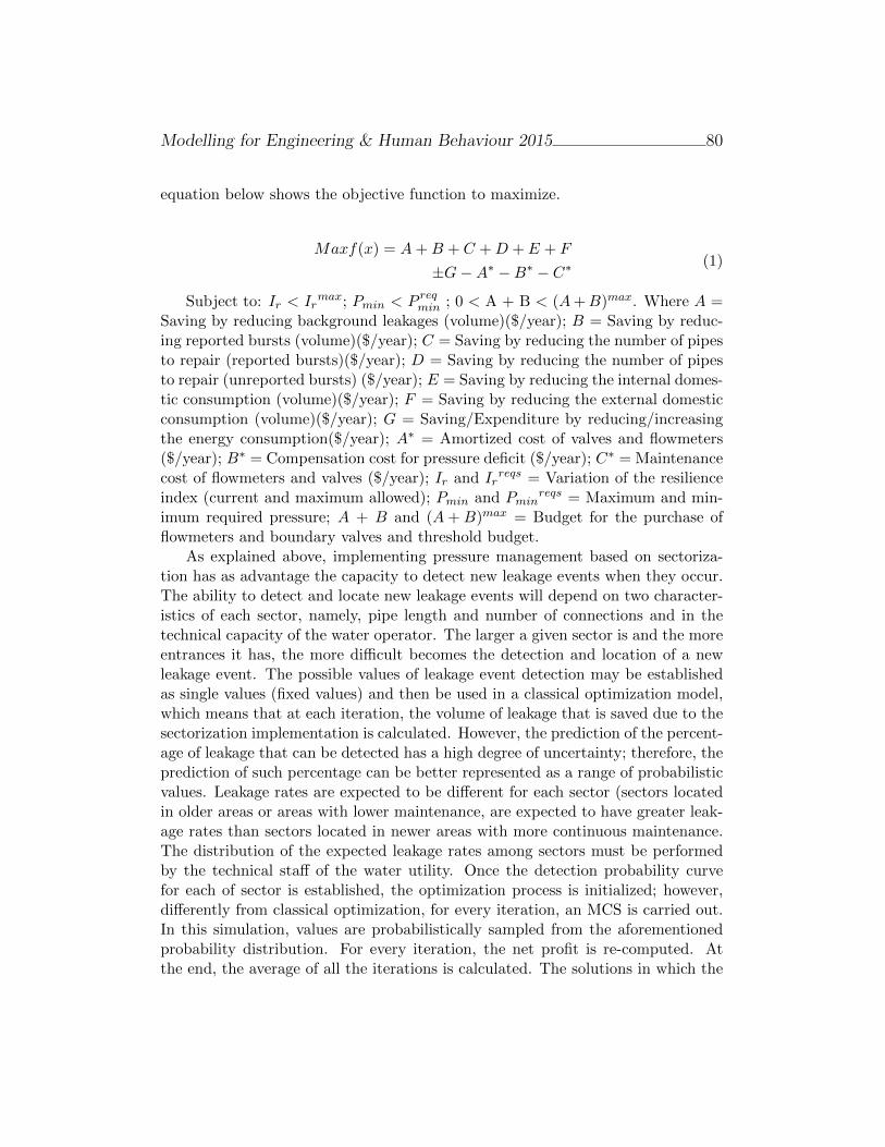
Modelling for Engineering & Human Behaviour 2015 80
equation below shows the objective function to maximize.
Maxf(x) = A + B + C + D + E + F
±G−A∗ −B∗ − C∗ (1)
Subject to: Ir < Irmax; Pmin < P req
min ; 0 < A + B < (A+B)max. Where A =Saving by reducing background leakages (volume)($/year); B = Saving by reduc-ing reported bursts (volume)($/year); C = Saving by reducing the number of pipesto repair (reported bursts)($/year); D = Saving by reducing the number of pipesto repair (unreported bursts) ($/year); E = Saving by reducing the internal domes-tic consumption (volume)($/year); F = Saving by reducing the external domesticconsumption (volume)($/year); G = Saving/Expenditure by reducing/increasingthe energy consumption($/year); A∗ = Amortized cost of valves and flowmeters($/year); B∗ = Compensation cost for pressure deficit ($/year); C∗ = Maintenancecost of flowmeters and valves ($/year); Ir and Ir
reqs = Variation of the resilienceindex (current and maximum allowed); Pmin and Pmin
reqs = Maximum and min-imum required pressure; A + B and (A + B)max = Budget for the purchase offlowmeters and boundary valves and threshold budget.
As explained above, implementing pressure management based on sectoriza-tion has as advantage the capacity to detect new leakage events when they occur.The ability to detect and locate new leakage events will depend on two character-istics of each sector, namely, pipe length and number of connections and in thetechnical capacity of the water operator. The larger a given sector is and the moreentrances it has, the more difficult becomes the detection and location of a newleakage event. The possible values of leakage event detection may be establishedas single values (fixed values) and then be used in a classical optimization model,which means that at each iteration, the volume of leakage that is saved due to thesectorization implementation is calculated. However, the prediction of the percent-age of leakage that can be detected has a high degree of uncertainty; therefore, theprediction of such percentage can be better represented as a range of probabilisticvalues. Leakage rates are expected to be different for each sector (sectors locatedin older areas or areas with lower maintenance, are expected to have greater leak-age rates than sectors located in newer areas with more continuous maintenance.The distribution of the expected leakage rates among sectors must be performedby the technical staff of the water utility. Once the detection probability curvefor each of sector is established, the optimization process is initialized; however,differently from classical optimization, for every iteration, an MCS is carried out.In this simulation, values are probabilistically sampled from the aforementionedprobability distribution. For every iteration, the net profit is re-computed. Atthe end, the average of all the iterations is calculated. The solutions in which the

Modelling for Engineering & Human Behaviour 2015 81
simulation results meet all the restrictions are marked as valid, and are used asfeedback to generate new solutions. The rest of the solutions are discarded.
4 Example of Implementation
To exemplify the methodology, it is implemented over a fraction of the WSN ofManagua city, Capital of Nicaragua. First, the supply trunk was identified, then,a set of 21 sectors, with pipe length between 3 and 34 km and with their respectivecandidate pipes (47 in total) were established. From the 21 sectors, six had onesingle entrance and the rest a set of 2-4 candidate pipes. The maximum differenceof elevation allowed between the nodes of each sector was set at 20 meters. As resultof the optimization of entrances/boundary valves, 35 flowmeters and 12 valves wereallocated. The annual net profit (savings - expenditures) resulted 72.397 $/year.If only background leakage reduction is considered among the benefits, the projectwould be infeasible.
5 Conclusion
In this paper we put in place a framework to account the benefits of sectorization,beyond only considering the benefits in terms of background leakage reduction. Asit is shown in the implementation example, by considering benefits as: savings byreducing reported leakage; savings by reducing unreported detectable leakage; sav-ings by reducing the number of pipes to repair (reported and unreported leakage)and savings due to reduction of domestic consumption (internal and external), thebalance Savings/Investment can be extremely different than when only background
Modelling for Engineering & Human Behaviour 2015 82
leaks are taken into consideration. In the presented example, the net profit ob-tained by implementing the proposed methodology is 72.397 $/year, significantlyabove the result obtained by only considering the reduction of background leakagesand energy, in which case, the project is infeasible. This work introduces novelconcepts to the sectorization research field, namely, Social Network CommunityDetection algorithms and MCS. With the first one, along with a merging processproposed in this work, it is possible to define sectors in WSNs depending of atrunk network. With MCS it is possible to take into consideration the inherentuncertainty in the prediction of new leakage events detection within the processof optimization of the entrances/boundaries valves. This is the first sectorizationresearch work that entails an analysis of the effect of sectorization layouts over thedetection of leakage events, and therefore we hope that the same could providenew guidelines for researchers and professionals involved in the WSN sectorizationresearch field.
References
[1] Blondel, V., Guillaume, J.L, Lambiotte, R. & Lefebvre, E. Fast unfolding ofcommunities in large networks Journal of Statistical Mechanics: Theory andExperiment, 10, pp. 10008, 2008.
[2] Campbell, E., Izquierdo, J., Montalvo, I., Ilaya-Ayza, A., Perez-Garcıa, R.& Tavera, M. A Flexible methodology to sectorize water supply networksbased on social network theory concepts and on multi-objective optimization.Journal of Hydroinformatics, 2015 (in press).
[3] Newman, M.Finding community structure in networks using the eigenvectorsof ma-trices. Physical Review E, 74(3), 2006.
[4] May, J. Leakage, pressure and control. In BICS International Conference onLeakage Control Investigation in Underground Assets, 1994, London, UK
[5] Lambert, A. & Lalonde, A.Using practical predictions of economic interven-tion frequency to calculate short run economic leakage level, with or withoutpressure management. Proceedings of IWA Specialised Conference ’Leakage2005’, Halifax, 2005, Nova Scotia, Canada.
[6] Thornton, J. & Lambert, A. Recent advances in understanding pressure: burstfrequency relationships. Update note (PowerPoint) for water loss task forcemembers, 2008. From [email protected]
Analysis of a class of discrete SIR epidemicmodel
B. Canto∗, C. Coll and E. SanchezInstituto de Matematica Multidisciplinar
Universitat Politecnica de Valencia, Camı de Vera s/n 46022 Valencia Spain
Deterministic models are represented by differential equations or differ-ence equations and therefore are associated equilibrium points. In this work,we develop a model with discrete age scale and discrete-time to analyze anepidemic with three states where each state is also subdivided in three com-partments depending on the age. The associated model assumes that thechain of infection and recovery is described as happening in discrete-timesteps, where each step is the interval between an individual acquiring infec-tion and passing it on to the next infected. Thus, the SIR model is describedby a discrete-time nonlinear system and it has unknown parameters whichdepend on the considered epidemic. This model is denoted by SIR(p) andit is a structured model, where each state is subdivided in: susceptible in-dividuals Si, infected individuals Ii and recovered individuals Ri at the i-thage compartment, for i = 1, 2, . . . ,m. The size of the population remainsconstant to N and an entry of new individuals proportional β(k)N state isadded to S1. The parameters involved in the model are as follows: Survivalrate: pi, qi and ri are the rate of survival individuals of Si, Ii and Ri, re-spectively. Change of compartment without changing the variable: σi, µi andνi are the rate of individuals becoming Si / Si+1, Ii / Ii+1 and Ri / Ri+1.Change of compartment with changing the variable: εi and δi are the rate ofsusceptible and infected individuals who pass from compartment i to i + 1.
Finally, the exposition rate and the recovered rate at time k are αiIi(k)
Nand
γi, respectively.
∗e-mail: [email protected]
83
Modelling for Engineering & Human Behaviour 2015 84
Then the model is of the form x(k + 1) = f(x(k),p), k ∈ Z wherex(k) ∈ Rn×n is the state vector, p is the parameter vector and f : Rn → Rn
is a continuously differentiable function in Rn.In the modeling process is important to know the behavior of the system
solution in a neighborhood of an equilibrium point. This allows us to deducewhether the disease will disappear, will be endemic or epidemic will growto generate a pandemic. In this way, we will use a linear approximationSIRL(p). First, the existence of the equilibrium points is studied. Since thepopulation size remains constant for all k
β(k)N = N −3∑
i=1
piSi(k)−3∑
i=1
qiIi(k)−3∑
i=1
riRi(k),
we obtain the disease-free equilibrium point Pf = (Sf1 , 0, 0, S
f2 , 0, 0, S
f3 , 0, 0)
given by
Sf1 =
N(1− p2 + σ2)(1− p3)
$; Sf
2 =σ1N(1− p3)
$; Sf
3 =σ1σ2N
$,
where $ = (1− p2 + σ2 + σ1)(1− p3) + σ2σ1.If we linearize around this point we obtain a linear approximation of
the initial system SIR(p) given by x(k + 1) = A(p)x(k) + b, being x(k) = S(k)I(k)R(k)
, A(p) the coefficient matrix that contains all the parameters of
the system and b = (N 0 0 0 0 0 0 0 0)T .In this work, the identifiability property of our model is analyzed in order
to confirm the possible identifiable parameters of the model from a givendata set. This analysis identifies the parameters or the relationship betweenparameters which are accessible from an input-output pair. In the last years,a great variety of works have been developed for the identifiability of severalmathematical models [1, 2] and [3].
Thus, a model is identifiable if the relationship between the set of possibleparameter values and the set of possible input-output behaviors is one-to-one. That is, given two parameter vectors p, p the equation xp(k) = xp(k)has only the solution p = p.
From the solution of the system SIRL(p), x(k) = Ak(p)x(0)+k−1∑i=0
Ai(p)b,
and using different initial conditions x(0), we can identify all the parameters
Modelling for Engineering & Human Behaviour 2015 85
except p1. The non-identifiability of p1 is therefore due only to the conditionthat the population is constant N at each time.
After solving the identifiability problem we obtain a model designed torepresent theoretical concepts, and to serve as bases for devising quantitativerelations and for predicting properties. By solving the identifiability prob-lem we guarantee that the model parameters can be estimated under idealconditions. In the next step, we will need to design a process to estimate theparameters that can be identified.
The usual estimation methods include the projection algorithm, gradientalgorithm and least squares algorithm, [4, 5]. In the estimation process willassume that for a given system the value of the parameters are not known,but we have recorded inputs and outputs over a time interval. So, considerpi = p, qi = q, ri = r, σi, µi and νi, i = 1, 2, 3, and εi and δi, i = 1, 2, areknown and the collection of observed dates given by
ob(k) = (S1(k) S2(k) S3(k) I1(k) I2(k) I3(k)R1(k) R2(k) R3(k))T ,
k = 1, 2, . . . , K, K ≥ 1. We will estimate relevant epidemiological pa-rameters as the transmission rates and the recovery rates, that is, p =(f1 f2 f3 γ1 γ2 γ3)T .
So, we rewrite the initial system as follows
x(k + 1) = M(k)p +N(k)
being matrices M(k) and N(k) obtained after the reorganization of the linearsystem SIRL(p).
Denote by e(i) = (ob(i) − x(i))T (ob(i) − x(i)), i = 1, . . . , K, and defineeK = col(e(i))K−1
i=0 , dK = col(d(i))Ki=1 = col(ob(i) − N(i − 1))Ki=1, and HK =col(M(i))K−1
i=0 .From K observed dataset we want estimate the value of p, that is, we can
find the parameter vector which minimizes to the quadratic cost function
J(K) =1
2
K∑i=1
e(i)T e(i) =1
2eTKeK =
1
2(dK −HKp)T (dK −HKp).
And we show that if there exists k0 such that Ii(k0) 6= 0, i = 1, 2, 3, thenthe solution from K observations with K > k0 is pK = (HT
k HK)−1HTKdK .
In addition, if there exists k0 such that Ii(k0) 6= 0, i = 1, 2, 3 then
Modelling for Engineering & Human Behaviour 2015 86
if ‖dK‖ <1
ρ(S−1K )
√ρ(SK)
then ‖pK‖ < 1,
being pK = S−1K HT
KdK the parameter which minimizes the problem associ-ated with K observation data.
If we add one observation ob(K+1), using a discrete-time variable systempK+1 = AKpK+BK , K ≥ 1 whereAK = S−1
K+1SK andBK = S−1K+1M(K)Td(K+
1), being SK = HTKHK , we get convergence conditions guaranteeing the suc-
cession of obtained parameters.Thus, assume that there exists k0 such that Ii(k0) 6= 0, i = 1, 2, 3, K > k0,
and consider the observation data such that
‖ob(K + 1)− x(K + 1)‖ < ε
ρ(S−1K )ρ(MT (K)M(K))
,
for some ε > 0. Then‖pK+1 − pK‖ < ε.
Acknowledgements: This research was partially supported by Ministerio deEconomıa y Competitividad under grant MTM2013-43678-P.
References
[1] Ben-Zvi A., McLellan P.J. and McAuley K.B., Identifiability of Linear Time-Invariant Differential-Algebraic systems. 2. The Differential-Algebraic Ap-proach, Ind. Eng. Chem. Res. 43(5): 1251–1259, 2004.
[2] Canto B., Coll C. and Sanchez E, Parameter identification of a Class of Eco-nomical Models, Discrete Dynamics in Nature and Society ID 408346, 1-12,2010.
[3] Canto B., Coll C. and Sanchez E, Identifiability of a class of discretized linearpartial differential algebraic equations, Math. Problems Eng. 1-12, 2011.
[4] Ding F., Liu P.X. and Liu G., Multiinnovatiovation Least-Squares Iden-tification for System Modeling, IEEE TRansaction on Systems,Man, andCybernetics-Part B: Cybernetics 18(3): 767–778, 2010.
[5] Malik M.B.and Salman M., State-space least mean square, Digital SignalProcessing 18: 334-345, 2008.
Modeling Plant Virus Propagation with Delays
Mark Jackson [ ∗, Benito M. Chen-Charpentier [ †
([) Department of Mathematics, University of Texas at Arlington, Arlington, TX 76019-0408,
November 30, 2015
1 Introduction
Plants are essential to not only man’s existence, but to every species onEarth. Sometimes, plants become infected with a disease. There are manydifferent ways that a plant may contract a disease. One of which is bacterial.For example, Magnaporthe oryzae is a bacteria that causes rice blast whichcan cause rice production to decrease up to 90 percent [4]. Also, a plant maybecome infected with a fungal disease. One such fungus is Botrytis cinerea,and it destroys the fruits the plant produces [10]. In this paper, we willbe interested in plant viruses and their dynamics. In order to work with theviruses, we must first understand how they replicate. For a virus to replicate,it must invade a healthy cell and use the cell’s DNA or RNA to reproduce.The infected cell bursts and several copies of the virus exit.The new virusparticles infect other cells. The viruses continue this process until there areno more healthy cells to invade. Different virus processes have been widelystudied. See for example [2], [12], [11], and [17].
Plant viruses cause many diseases some of which that affect many plantsall over the world. For instance, the Citrus tristeza virus once wiped outmillions of trees in Brazil [7]. But in order for an infected plant to infectanother, a virus from an infected plant must come in contact with a healthyplant. This may happen in several different ways. For example, a fieldworker might contact the juices of an infected plant and contact a healthy
∗e-mail:[email protected]†e-mail:[email protected]
87

Modelling for Engineering & Human Behaviour 2015 88
plant. Or maybe the interaction is more organic in that an infected plantmight have its juices fall directly onto a plant underneath it. Another, andthe most common, way for the transference is by an insect vector. Insectvectors transmit more than 70 percent of all known plant viruses [7]. Manyvectors that transport these viruses include aphids, whiteflies, leafhoppers,etc.
There are many ways that plant viruses interact with the vectors, but inthis paper we are concerned with circulative, persistent transmission. Thistransmission works in the following way. The vectors consume sap from aninfected host through their stylets. The viruses in the sap enter the salivaryglands, circulates within the vector, and then causes infection. This processcan take up to a few hours or up to a few days depending on the insect-vectorinteraction. The vector will hold the infection for the rest of it’s life. Whenthe infected vector contacts a healthy plant, some virus particles leave thevector and invade the plant [15, 16, 13]. Once the virus has circulated andpropagated throughout the plant, the plant may use defense mechanisms tocombat the virus. On example is by antiviral RNA silencing, a process bywhich slicing or translation repression of viruses occurs [8].
Many physical and biological processes (gestation, maturation, reproduc-tion, infection) take time to complete. In the case of a viral infection, it takestime for a virus to invade a cell, reproduce, and spread in order throughoutthe host. This process time is a delay time. Processes with delay timescan be modeled using delay differential equations (DDE). Delay times canchange the dynamics of the model. For example, delays may change the so-lutions, cause discontinuities in the derivative, introduce oscillations, affectuniqueness, or change the stability. Despite the complications and numericaldifficulties, results are more realistic from the biological and physical pointsof view. The effects of the delay times are highly coupled with the parametersof the model. See for example [6, 9].
Although there are many models that describe in interaction betweenvectors and humans, there are not as many that describe the relationshipbetween plants and vectors. In this paper, we construct a model assumingthat the virus gets transmitted by plant and insect contact, and is modeledusing Holling type II [1], since insects can only bite a limited number ofplants. In [15] a similar model is presented that also consider that infectioncan be transmitted from plant to plant. We do not consider such transmissionbecause in [16] it is said it is not common.

Modelling for Engineering & Human Behaviour 2015 89
2 Mathematical Model
In this model we do not consider a specific virus, plant, or insect vector, butwe make the following assumptions.
There are three populations of plants: Susceptible, S, healthy but subjectto be infected by the virus, Infective, I, already infected by the virus, andRecovered, R. Each of these variables describe their respective populationat time, t. The total number of plants will be denoted by the fixed positiveconstant K, K = S + I + R. It is reasonable to assume K is fixed, becausewhen a plant dies by the virus or natural death in farms, it is usually replacedwith a new healthy plant.
For the insect vectors, there will be two populations : Susceptible, X, andInfective, Y . Each of which describe the populations at time, t, as well. Thetotal number of insects will be denoted by the constant, N, N=X+Y. Also,the rate at which the insects enter the system, by birth or immigration, isconstant. There is no vertical transmission of the virus, and vectors cannottransmit the virus to another vector. In addition, vectors do not get killedby the virus nor do they defend against it. The vector will keep the virus forit’s lifespan and does not recover. The infective insects do not get sick fromthe virus, they are just carriers.
As far as the interaction between the insects and the plants, an infectedinsect vector can only infect a susceptible plant. The only way for the vectorto become infected is through coming in contact with an infected plant. Theinteraction between vector and plant is of predator-prey Holling type 2 [1].
The differential equations for this model are
dS
dt= µK + dI − µS − βY
1 + αYS
dI
dt=
βY
1 + αYS − (d+ µ+ γ)I
dR
dt= γI − µR
dX
dt= Λ− β1IX
1 + α1I−mX
dY
dt=
β1IX
1 + α1I−mY,
where µ is the natural death rate of the plants, d is the death rate of infected
Modelling for Engineering & Human Behaviour 2015 90
plants due to the disease, α is the saturation constant of plants due to vectors,β is the infection rate of plants due to vectors, γ is the recovery rate of plants,Λ is the replenishing rate of vectors (birth and/or immigration) β1 is infectionrate of vectors due to plants, α1 is the saturation constant of vectors due toplants and m is the natural death rate of vectors.
To get a more realistic model, we consider two delays, τ1, which is time ittakes a plant to become infected after contagion and τ2, the time it takes avector to become infected after contagion. The model with the two discretedelays, assuming that the total populations of plants and vectors are constantso R and X can be eliminated, is
dS
dt= µ(K − S)− βY (t− τ1)
1 + αY (t− τ1)S(t− τ1) + dI
dI
dt=
βY (t− τ1)1 + αY (t− τ1)
S(t− τ1)− ωI
dY
dt=
β1I(t− τ2)1 + α1I(t− τ2)
(Λ
m− Y (t− τ2))−mY.
The delay differential equations are solved numerically [3, 14] and ana-lyzed numerically using dde-biftool [5].
3 Discussion
We presented two plant virus propagation models, one with no delays andthe other with two delays. In the case where the basic reproduction numberwas less than 1, we notice that the introduction of delays introduces sig-nificant changes in the solution for the susceptible, infected, and recoveredplants, including a longer time to approach approach the disease free equi-librium point and oscillations. For the insect populations, there is a smallerchange in the solutions. When the basic reproduction number was greaterthan 1, however, the endemic steady state becomes stable and the diseasefree becomes unstable and this also corroborated by the numerical calcula-tions. The natural death rate of the vector was chosen as the continuationparameter. We changed the value of the natural death rate of the vector,since it is one value that can be modified by the use of pesticides, predatorsor other vector control means. Furthermore, the results show that it is not
Modelling for Engineering & Human Behaviour 2015 91
necessary to eliminate the vector completely, only to increase its death rateto control an epidemic.
The study of the stability of both equilibrium points of the delay dif-ferential equation system, has to be done numerically. We used the codedde-biftool [5], which also allows the variation of some parameters and willapproximate the location of bifurcation points.
We ran simulations for different values of the delay times, and similarresults were obtained. In particular, we increased the delay time for thevirus-insect interaction. The solutions were slightly different but the diseasefree equilibrium was stable for R0 < 1 and unstable when R0 > 1. Likewise,the endemic equilibrium was stable for R0 > 1 and unstable when R0 < 1.
In addition, there is a Hopf bifurcation of the disease free branch atm = .2974 when τ1 = 24, τ2 = 1, but the some populations at the bifurcatedbranch are negative, so the branch is unrealistic. The same is true for theHopf bifurcation point on the endemic equilibrium branch. So there are noperiodic solutions.
Delayed model is more realistic because it takes into account the timebetween the release of a factor and its absorption and its effect.
Although a specific plant, insect vector, and virus was not considered,the parameters can be modified to fit a particular situation.
References
[1] L. Allen, An Introduction to Mathematical Biology. Upper Saddle River,New Jersey, Pearson-Prentice Hall, 2007.
[2] R. M. Anderson and R. M. May, Infectious Diseases of Humans. Oxford,Oxford University Press, 1991.
[3] A. Bellen and M. Zennaro, Numerical Methods for Delay Differentialequations. New York, Oxford University Press, 2005.
[4] R. K. Ellur et al., Improvement of Basmati rice varieties for resistanceto blast and bacterial blight diseases using marker assisted backcrossbreeding, Plant Science Volume 242: 330–341, 2015.
[5] K. Engelborghs et al., DDE-BIFTOOL: a Matlab package for bifurcationanalysis of delay differential equations. Leuven, Belgium, Department ofComputer Sciences, Free University, 2001.
Modelling for Engineering & Human Behaviour 2015 92
[6] T. Erneux, Applied Delay Differential Equations. New York, Springer,2009.
[7] A. Fereres, Insect vectors as drivers of plant virus emergence, CurrentOpinion in Virology, Volume 10: 42–46, 2015.
[8] B. Ghoshal and H. Sanfacon, Symptom recovery in virus-infected plants:Revisiting the role of RNA silencing mechanisms, Virology, Volumes479–480: 167–179, 2015.
[9] Y. Kuang, Delay Equations with Applications to Population Dynamics.San Diego, Academic Press, 1993.
[10] S.V. Leontopoulosa et al. Effect of Different Formulations of Polyphe-nolic Compounds Obtained from OMWW on the Growth of SeveralFungal Plant and Food Borne Pathogens. Studies in vitro and in vivo.Agriculture and Agricultural Science Procedia, Volume 4: 327-337, 2015.
[11] M.A. Novak, Virus Dynamics: Mathematical Models of Immunologyand Virology. New York, Oxford University Press, 2000.
[12] A.S. Perelson, D.E. Kirschner and R. De Boer. Dynamics of HIV Infec-tion of CD4+ T-cells, Math. Biosci. Volume 114: 81–125, 1993.
[13] Y. Robert and D. Bourdin, Virus and Virus-like Diseases of Potatoesand Production of Seed-Potatoes. Dordrecht, Springer Science, 2001.
[14] L. F. Shampine, I. Gladwell, and S. Thompson, Solving ODEs withMATLAB., Cambridge, Cambridge University Press, 2003.
[15] R. Shi, H. Zhao, and S. Tang. Global Dynamic Analysis of a Vector-Borne Plant Disease Model, Advances in Difference Equations, Volume2014:59, 2014.
[16] A. Whitfield et al. Insect vector-mediated tranamission of plant viruses,Virology, Volumes 479–480: 278–289, 2015.
[17] D. Wodarz, Killer Cell Dynamics: Mathematical and ComputationalApproaches to Immunology. New York, Springer, 2007.
A Resource-constrained scheduling problem tooptimize the use of resources in a distribution
center with genetic algorithms.
David Cipres[ ∗, Lorena Polo[, and Pablo Artaso[
([) Aragon Institute of Technology (ITAINNOVA),
Marıa Luna 7-8, 50018 Zaragoza, Spain
November 30, 2015
1 Introduction
The complexity of the planning process in a distribution center is high dueto the large number of variables and possible combinations that may affect inthe development process. Different trends in manufacturing and distributionhave made the order picking process more and more important and complex.These new trends cause high variability in the workload, on the other handthe available resources are limited and they have to be planned in advance.Sometimes the available resources are adjusted to the company needs; othertimes available resources are below what is needed and could lead to problemin the overall operation.
Although the distribution centers have a key role in the success, or failure,in supply chains [Frazelle, 2002] at the design stage, there is no systematic orscientific approach to the physical design of ware-houses [Goetschalckx et al.,2002, Baker, 2008]. In the absence of a defined and accepted methodologywarehouse designers develop their own methods [Oxley, 1994]. In the litera-ture review there are different examples using meta heuristics in the transportand warehousing domain like [Escuın et al., 2012, Sicilia et al., 2015, Royo
∗e-mail: [email protected]
93
Modelling for Engineering & Human Behaviour 2015 94
et al., 2015]. But still there is an enormous gap between the published ware-house research and the practice of warehouse design and operations [Gu et al.,2007]. For a typical warehouse, the cost of order picking is estimated to beas much as 55% of the total warehouse operating expense [Tompkins et al.,2010].
2 Problem description
To solve this problem we propose a method that fits the complexity of thepicking process with high variability and integrated with other warehous-ing operations. In this paper we focus in the resource allocation to tasksin a distribution center. Scheduling and Resource Allocation are tradition-ally considered as very complex business problems. The challenge is how toschedule operational resources according to the operational flow in a distribu-tion center in specified time intervals. The main variables are the resourcesassigned to tasks and work intervals. To solve this assignation problem, wehave implemented a genetic algorithm to get a fast and feasible solution. Inaddition, outputs are compared with the results obtained by a linear pro-gramming model (LP) solved by an optimization library. The objective fromthis model is to define a decision-making system for planning task and re-source assignment with the required service level in the distribution centers.The main constrains identified are that we have to maintain the service level(Truck schedule time table). There is a limitation in the use of resources(operators, forklifts, docks). And finally we have to maintain the precedencesequence among the tasks.
2.1 Model description
The complexity of this problem could be high, it is a NP-Hard problem.For little instances, it could be solved with standard lineal programmingtechniques like Simplex Method. In this case the dimension of the problemis big, the number of scheduled task in one day is bigger than 300, the numberof operators could be 50. The genetic algorithm is a heuristic, it is routinelyused to generate useful solutions to optimization and search problems withno size limitation. The Chromosome representation in our algorithm has fivegenes: Orders (O), Tasks (T ), tEams (E), time Period (P ) and Quantity ofresources (Q).

Modelling for Engineering & Human Behaviour 2015 95
Phase Description
Initialization A first theoretical solution is computed taking onlyprecedence constraints and temporal restrictions of thetasks into account.
Selection The selection of the individuals who are going to repro-duce.
Cross-Over The Cross-Over operation mix the genes from two par-ents in one generation, and creates two new child calledoffspring.
Mutation An order which belongs to a solution can be mutated inthree distinct ways
Evaluation Schedule performance is measured in terms of resourceavailability and length of the order execution.
Table 1: Genetic Algorithm phases
One order is composed by tasks. Each task from one Order has to beassigned to a Team with skill to perform the task in one period of time. Thequantity of resources assigned is defined by Q. The algorithm schedules tasksfrom one initial plan and evolves considering precedence and resource con-straints. The selected algorithm is a Steady-State Genetic algorithm becauseoverlaps populations. The size of the population remains constant. Then,once the offspring has been added, the population is truncated by randomlyremoving two chromosomes from the ten per cent worst evaluated ones. Thepopulation size used in the problems depends on the nature of the problem.In this case the population size is 50.
Tasks have precedence relationships between them so so each task cannot start until its predecessors have completely finished. In addition, thereare temporal restrictions. That is to say that some tasks can be blocked,other can be delayed and other can be brought forward. In addition, thereare several resources types with their own temporal restrictions and task-resource dependencies.
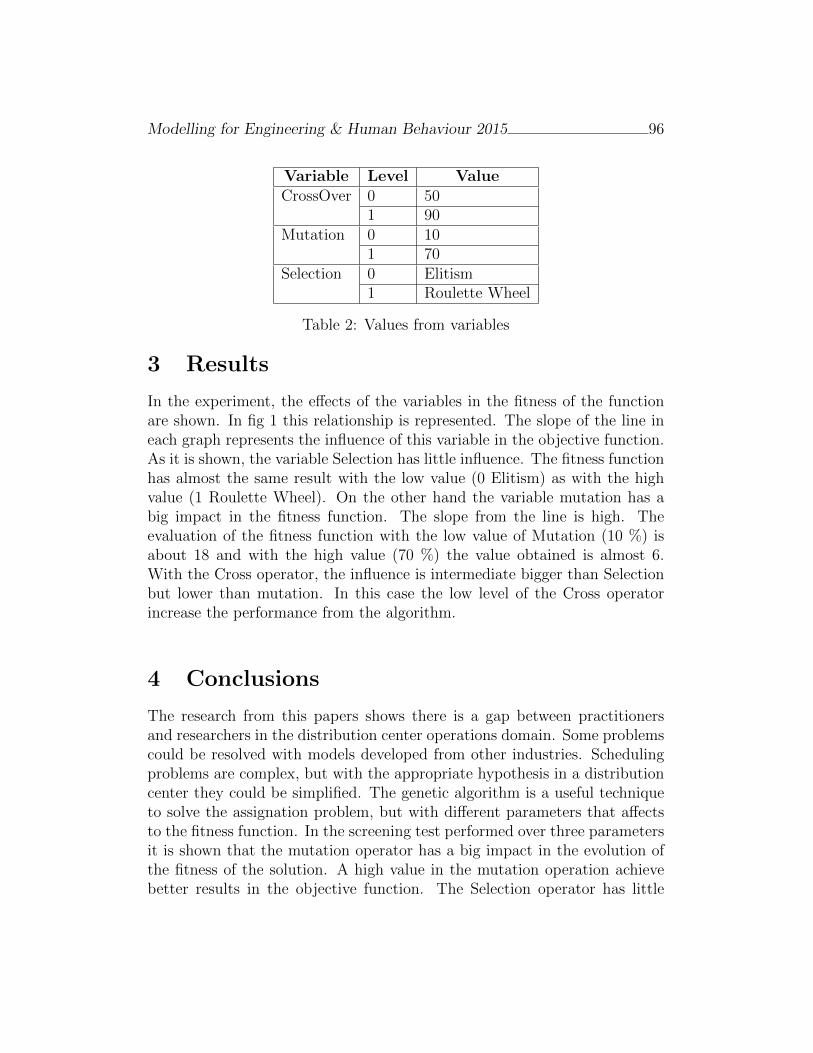
Modelling for Engineering & Human Behaviour 2015 96
Variable Level ValueCrossOver 0 50
1 90Mutation 0 10
1 70Selection 0 Elitism
1 Roulette Wheel
Table 2: Values from variables
3 Results
In the experiment, the effects of the variables in the fitness of the functionare shown. In fig 1 this relationship is represented. The slope of the line ineach graph represents the influence of this variable in the objective function.As it is shown, the variable Selection has little influence. The fitness functionhas almost the same result with the low value (0 Elitism) as with the highvalue (1 Roulette Wheel). On the other hand the variable mutation has abig impact in the fitness function. The slope from the line is high. Theevaluation of the fitness function with the low value of Mutation (10 %) isabout 18 and with the high value (70 %) the value obtained is almost 6.With the Cross operator, the influence is intermediate bigger than Selectionbut lower than mutation. In this case the low level of the Cross operatorincrease the performance from the algorithm.
4 Conclusions
The research from this papers shows there is a gap between practitionersand researchers in the distribution center operations domain. Some problemscould be resolved with models developed from other industries. Schedulingproblems are complex, but with the appropriate hypothesis in a distributioncenter they could be simplified. The genetic algorithm is a useful techniqueto solve the assignation problem, but with different parameters that affectsto the fitness function. In the screening test performed over three parametersit is shown that the mutation operator has a big impact in the evolution ofthe fitness of the solution. A high value in the mutation operation achievebetter results in the objective function. The Selection operator has little
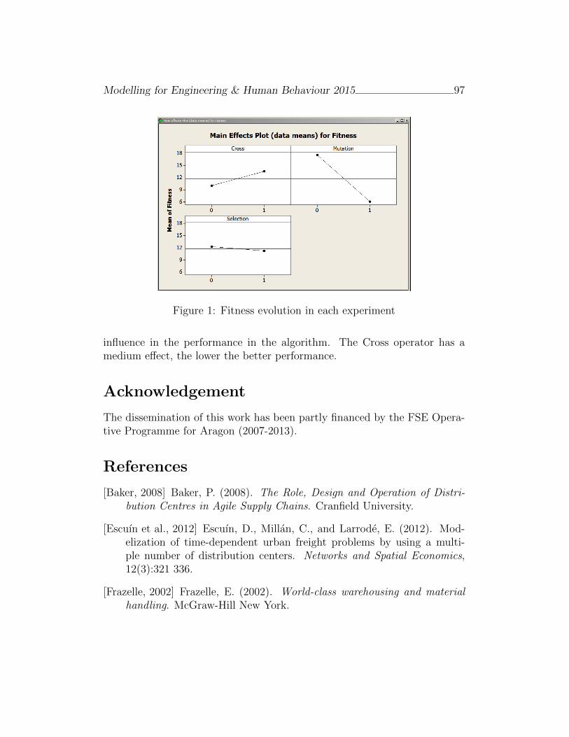
Modelling for Engineering & Human Behaviour 2015 97
Figure 1: Fitness evolution in each experiment
influence in the performance in the algorithm. The Cross operator has amedium effect, the lower the better performance.
Acknowledgement
The dissemination of this work has been partly financed by the FSE Opera-tive Programme for Aragon (2007-2013).
References
[Baker, 2008] Baker, P. (2008). The Role, Design and Operation of Distri-bution Centres in Agile Supply Chains. Cranfield University.
[Escuın et al., 2012] Escuın, D., Millan, C., and Larrode, E. (2012). Mod-elization of time-dependent urban freight problems by using a multi-ple number of distribution centers. Networks and Spatial Economics,12(3):321 336.
[Frazelle, 2002] Frazelle, E. (2002). World-class warehousing and materialhandling. McGraw-Hill New York.

Modelling for Engineering & Human Behaviour 2015 98
[Goetschalckx et al., 2002] Goetschalckx, M., Vidal, C. J., and Dogan, K.(2002). Modeling and design of global logistics systems: A review ofintegrated strategic and tactical models and design algorithms. EuropeanJournal of Operational Research, 143(1):1–18.
[Gu et al., 2007] Gu, J., Goetschalckx, M., and Mcginnis, L. (2007). Re-search on warehouse operation: A comprehensive review. EuropeanJournal of Operational Research, 177(1):1–21.
[Oxley, 1994] Oxley, J. (1994). Avoiding inferior design: The design of awarehouse is not a simple matter and the consequences of inadequatewarehouse planning cannot be overstated. Storage handling distribution,38:28.
[Rowley, 2000] Rowley, J. (2000). The principles of warehouse design. TheInstitute of Logistics & Transport, Corby.
[Royo et al., 2015] Royo, B., Fraile, A., Larrode, E., and Muerza, V. (2015).Route planning for a mixed delivery system in long distance transporta-tion and comparison with pure delivery systems. Journal of Computa-tional and Applied Mathematics.
[Sicilia et al., 2015] Sicilia, J. A., Quemada, C., Royo, B., and Escuın, D.(2015). An optimization algorithm for solving the rich vehicle routingproblem based on variable neighborhood search and tabu search meta-heuristics. Journal of Computational and Applied Mathematics.
[Tompkins et al., 2010] Tompkins, J., White, J., Bozer, Y., and Tanchoco,J. (2010). Facilities Planning. Wiley.
Dynamical tools for better understanding thestability of high-order methods for solving
nonlinear problems ∗
A. Cordero[ †, A.A. Magrenan‡, and Juan R. Torregrosa[
([) Instituto de Matematicas Multidisciplinar,
Universitat Politecnica de Valencia, Camino de Vera, s/n, 46022-Valencia, Spain
(‡) Universidad Internacional de La Rioja, Logrono, Spain
November 30, 2015
1 Introduction
In many branches of Science and Technology it is necessary to solve differentkinds of nonlinear equations or systems F (x) = 0, where F : X → Y , being Xand Y Banach spaces. The best known iterative scheme is Newton’s method
x(k+1) = x(k) − [F ′(x(k))]−1F (x(k)), k = 0, 1, . . .
but Traub’s scheme increases the order of convergence of Newton’s one, with-out a complex iterative formula
y(k) = x(k) − [F ′(x(k))]−1F (x(k)),x(k+1) = y(k) − [F ′(x(k))]−1F (y(k)), k = 0, 1, . . .
(1)
where F ′(x) denotes the Frechet derivative of F . This scheme can be suc-cessfully used, with third-order convergence, on nonlinear problems.
∗This research was partially supported by Ministerio de Economıa y CompetitividadMTM2014-52016-C2-1, 2-P.†e-mail: [email protected]
99
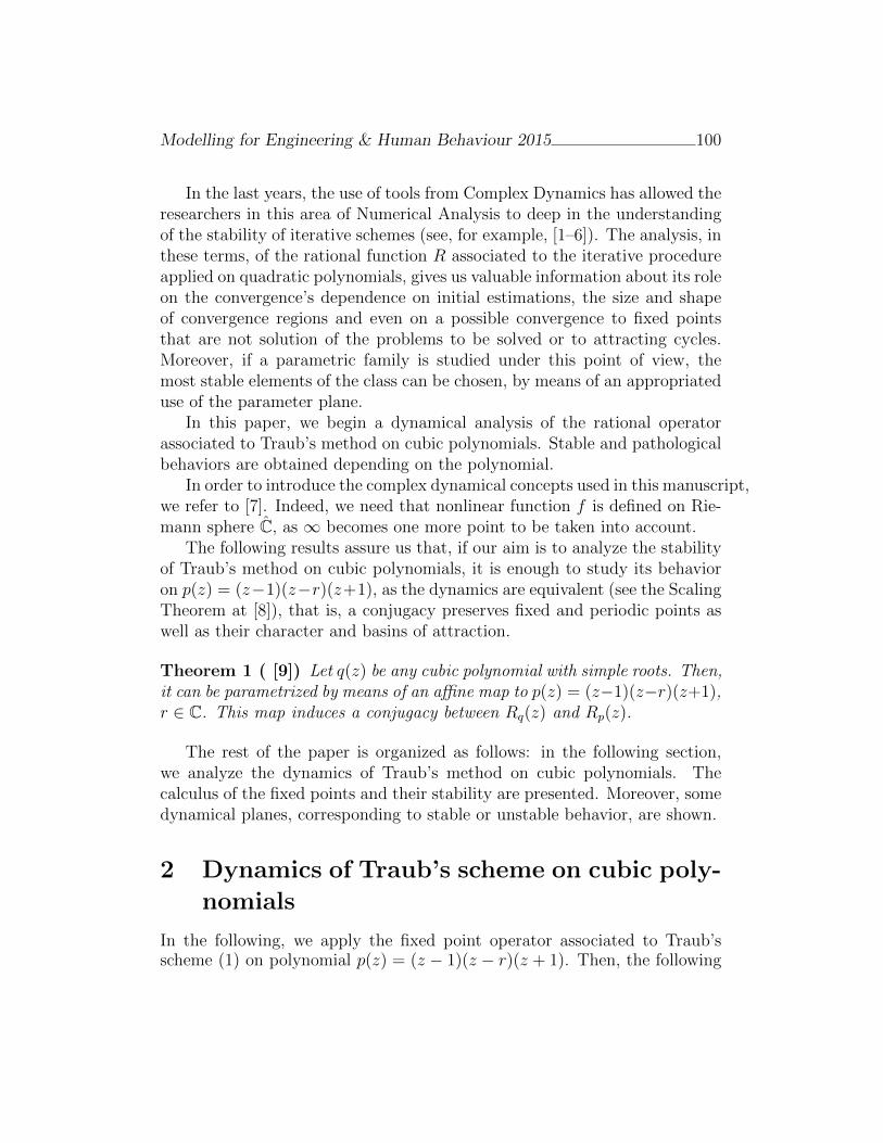
Modelling for Engineering & Human Behaviour 2015 100
In the last years, the use of tools from Complex Dynamics has allowed theresearchers in this area of Numerical Analysis to deep in the understandingof the stability of iterative schemes (see, for example, [1–6]). The analysis, inthese terms, of the rational function R associated to the iterative procedureapplied on quadratic polynomials, gives us valuable information about its roleon the convergence’s dependence on initial estimations, the size and shapeof convergence regions and even on a possible convergence to fixed pointsthat are not solution of the problems to be solved or to attracting cycles.Moreover, if a parametric family is studied under this point of view, themost stable elements of the class can be chosen, by means of an appropriateduse of the parameter plane.
In this paper, we begin a dynamical analysis of the rational operatorassociated to Traub’s method on cubic polynomials. Stable and pathologicalbehaviors are obtained depending on the polynomial.
In order to introduce the complex dynamical concepts used in this manuscript,we refer to [7]. Indeed, we need that nonlinear function f is defined on Rie-mann sphere C, as ∞ becomes one more point to be taken into account.
The following results assure us that, if our aim is to analyze the stabilityof Traub’s method on cubic polynomials, it is enough to study its behavioron p(z) = (z−1)(z−r)(z+1), as the dynamics are equivalent (see the ScalingTheorem at [8]), that is, a conjugacy preserves fixed and periodic points aswell as their character and basins of attraction.
Theorem 1 ( [9]) Let q(z) be any cubic polynomial with simple roots. Then,it can be parametrized by means of an affine map to p(z) = (z−1)(z−r)(z+1),r ∈ C. This map induces a conjugacy between Rq(z) and Rp(z).
The rest of the paper is organized as follows: in the following section,we analyze the dynamics of Traub’s method on cubic polynomials. Thecalculus of the fixed points and their stability are presented. Moreover, somedynamical planes, corresponding to stable or unstable behavior, are shown.
2 Dynamics of Traub’s scheme on cubic poly-
nomials
In the following, we apply the fixed point operator associated to Traub’sscheme (1) on polynomial p(z) = (z − 1)(z − r)(z + 1). Then, the following
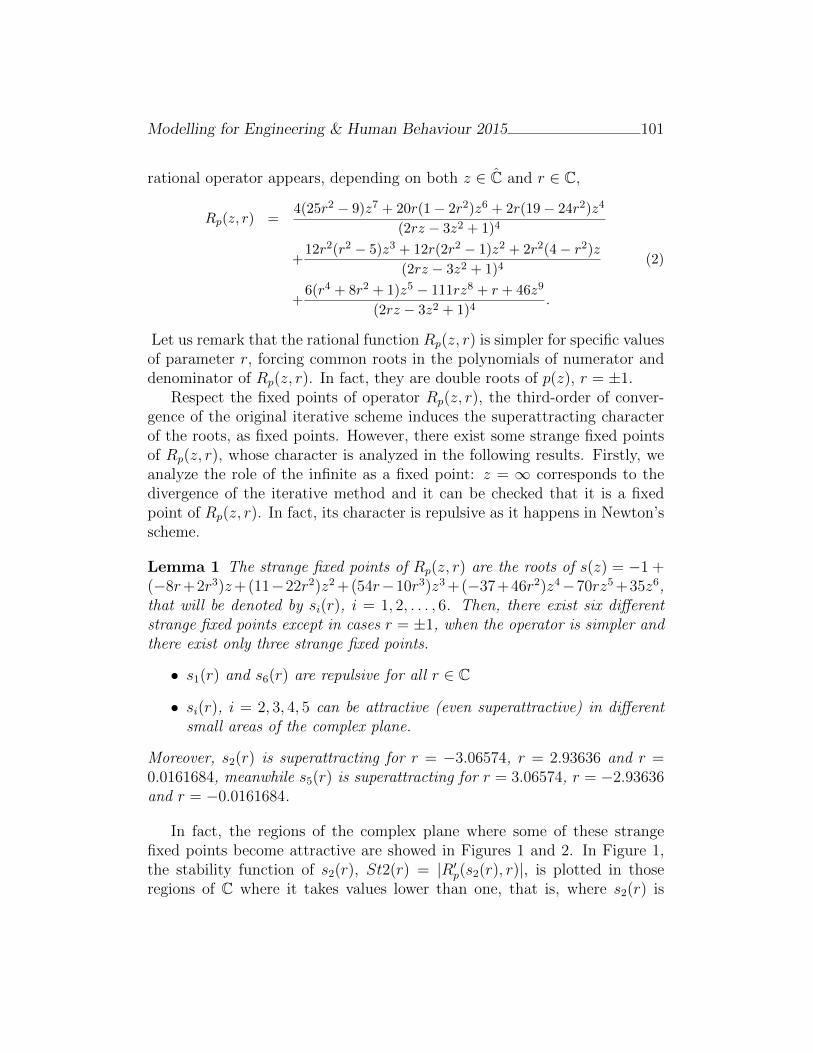
Modelling for Engineering & Human Behaviour 2015 101
rational operator appears, depending on both z ∈ C and r ∈ C,
Rp(z, r) =4(25r2 − 9)z7 + 20r(1− 2r2)z6 + 2r(19− 24r2)z4
(2rz − 3z2 + 1)4
+12r2(r2 − 5)z3 + 12r(2r2 − 1)z2 + 2r2(4− r2)z
(2rz − 3z2 + 1)4(2)
+6(r4 + 8r2 + 1)z5 − 111rz8 + r + 46z9
(2rz − 3z2 + 1)4.
Let us remark that the rational function Rp(z, r) is simpler for specific valuesof parameter r, forcing common roots in the polynomials of numerator anddenominator of Rp(z, r). In fact, they are double roots of p(z), r = ±1.
Respect the fixed points of operator Rp(z, r), the third-order of conver-gence of the original iterative scheme induces the superattracting characterof the roots, as fixed points. However, there exist some strange fixed pointsof Rp(z, r), whose character is analyzed in the following results. Firstly, weanalyze the role of the infinite as a fixed point: z = ∞ corresponds to thedivergence of the iterative method and it can be checked that it is a fixedpoint of Rp(z, r). In fact, its character is repulsive as it happens in Newton’sscheme.
Lemma 1 The strange fixed points of Rp(z, r) are the roots of s(z) = −1 +(−8r+2r3)z+(11−22r2)z2 +(54r−10r3)z3 +(−37+46r2)z4−70rz5 +35z6,that will be denoted by si(r), i = 1, 2, . . . , 6. Then, there exist six differentstrange fixed points except in cases r = ±1, when the operator is simpler andthere exist only three strange fixed points.
• s1(r) and s6(r) are repulsive for all r ∈ C
• si(r), i = 2, 3, 4, 5 can be attractive (even superattractive) in differentsmall areas of the complex plane.
Moreover, s2(r) is superattracting for r = −3.06574, r = 2.93636 and r =0.0161684, meanwhile s5(r) is superattracting for r = 3.06574, r = −2.93636and r = −0.0161684.
In fact, the regions of the complex plane where some of these strangefixed points become attractive are showed in Figures 1 and 2. In Figure 1,the stability function of s2(r), St2(r) = |R′p(s2(r), r)|, is plotted in thoseregions of C where it takes values lower than one, that is, where s2(r) is
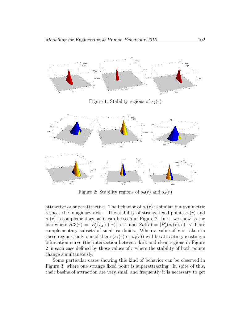
Modelling for Engineering & Human Behaviour 2015 102
Figure 1: Stability regions of s2(r)
Figure 2: Stability regions of s3(r) and s4(r)
attractive or superattractive. The behavior of s5(r) is similar but symmetricrespect the imaginary axis. The stability of strange fixed points s3(r) ands4(r) is complementary, as it can be seen at Figure 2. In it, we show as theloci where St3(r) = |R′p(s3(r), r)| < 1 and St4(r) = |R′p(s4(r), r)| < 1 arecomplementary subsets of small cardioids. When a value of r is taken inthese regions, only one of them (s3(r) or s4(r)) will be attracting, existing abifurcation curve (the intersection between dark and clear regions in Figure2 in each case defined by those values of r where the stability of both pointschange simultaneously.
Some particular cases showing this kind of behavior can be observed inFigure 3, where one strange fixed point is superattracting. In spite of this,their basins of attraction are very small and frequently it is necessary to get
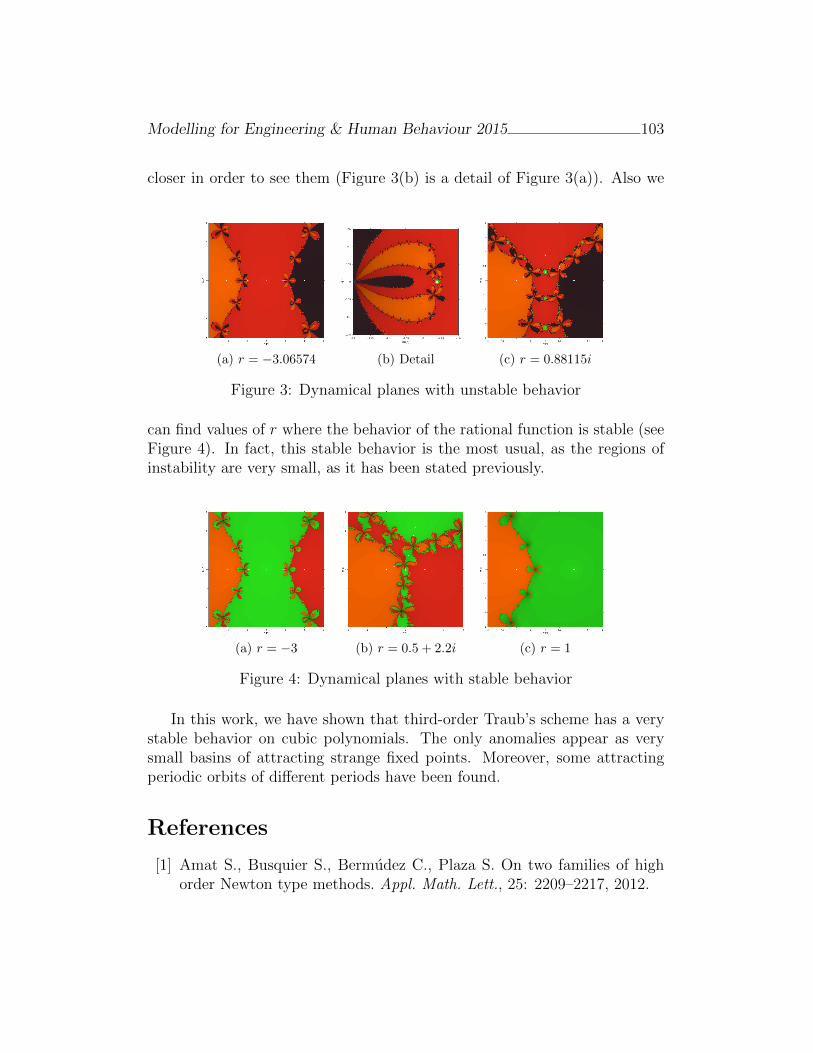
Modelling for Engineering & Human Behaviour 2015 103
closer in order to see them (Figure 3(b) is a detail of Figure 3(a)). Also we
(a) r = −3.06574 (b) Detail (c) r = 0.88115i
Figure 3: Dynamical planes with unstable behavior
can find values of r where the behavior of the rational function is stable (seeFigure 4). In fact, this stable behavior is the most usual, as the regions ofinstability are very small, as it has been stated previously.
(a) r = −3 (b) r = 0.5 + 2.2i (c) r = 1
Figure 4: Dynamical planes with stable behavior
In this work, we have shown that third-order Traub’s scheme has a verystable behavior on cubic polynomials. The only anomalies appear as verysmall basins of attracting strange fixed points. Moreover, some attractingperiodic orbits of different periods have been found.
References
[1] Amat S., Busquier S., Bermudez C., Plaza S. On two families of highorder Newton type methods. Appl. Math. Lett., 25: 2209–2217, 2012.

Modelling for Engineering & Human Behaviour 2015 104
[2] Chicharro F., Cordero A., Torregrosa J.R. Drawing dynamical and pa-rameter planes of iterative families and methods. The Sci. World J.,2013: Article ID 780153, 2013.
[3] Cordero A., Garcıa-Maimo J., Torregrosa J.R., Vassileva M.P., VindelP. Chaos in King’s iterative family. Appl. Math. Lett., 26: 842–848, 2013.
[4] Cordero A., Torregrosa J.R., Vindel P. Study of the dynamics of third-order iterative methods on quadratic polynomials. Intern. J. Comput.Math., 89(13-14): 1826–1836, 2012.
[5] Magrenan A. A. Different anomalies in a Jarratt family of iterative root-finding methods. App. Math. Comput., 233: 29–38, 2014.
[6] Neta B., Chun C., Scott M. Basins of attraction for optimal eighth ordermethods to find simple roots of nonlinear equation. App. Math. Comput.,227: 567–592, 2014.
[7] Blanchard P. Complex Analytic Dynamics on the Riemann Sphere. Bull.AMS, 11(1): 85–141, 1984.
[8] Amat S., Busquier S., Plaza S. Review of some iterative root-findingmethods from a dynamical point of view. Scientia, 10: 3–35, 2004.
[9] Roberts G., Horgan-Kobelski J. Newton’s versus Halley’s method: adynamical systems approach. Intern. J. Bifur. Chaos, 14: 3459–3475,2004.
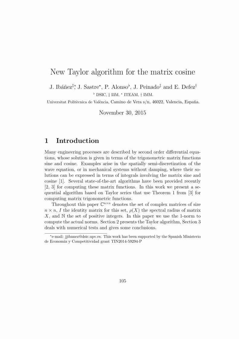
New Taylor algorithm for the matrix cosine
J. Ibanez‡∗, J. Sastre⋆, P. Alonso, J. Peinado‡ and E. Defez†
DSIC, ‡ I3M, ⋆ ITEAM, † IMM.
Universitat Politecnica de Valencia, Camino de Vera s/n, 46022, Valencia, Espana.
November 30, 2015
1 Introduction
Many engineering processes are described by second order differential equa-tions, whose solution is given in terms of the trigonometric matrix functionssine and cosine. Examples arise in the spatially semi-discretization of thewave equation, or in mechanical systems without damping, where their so-lutions can be expressed in terms of integrals involving the matrix sine andcosine [1]. Several state-of-the-art algorithms have been provided recently[2, 3] for computing these matrix functions. In this work we present a se-quential algorithm based on Taylor series that use Theorem 1 from [3] forcomputing matrix trigonometric functions.
Throughout this paper Cn×n denotes the set of complex matrices of sizen× n, I the identity matrix for this set, ρ(X) the spectral radius of matrixX, and N the set of positive integers. In this paper we use the 1-norm tocompute the actual norms. Section 2 presents the Taylor algorithm, Section 3deals with numerical tests and gives some conclusions.
∗e-mail: [email protected]. This work has been supported by the Spanish Ministeriode Economıa y Competitividad grant TIN2014-59294-P
105
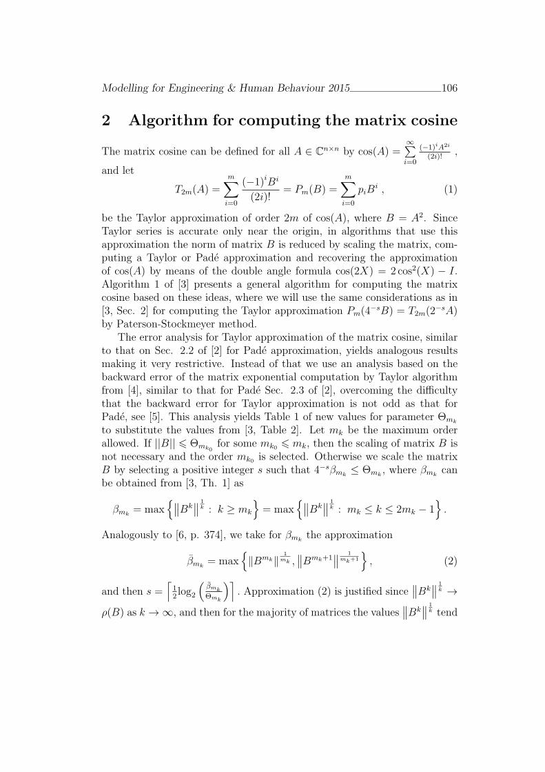
Modelling for Engineering & Human Behaviour 2015 106
2 Algorithm for computing the matrix cosine
The matrix cosine can be defined for all A ∈ Cn×n by cos(A) =∞∑i=0
(−1)iA2i
(2i)!,
and let
T2m(A) =m∑i=0
(−1)iBi
(2i)!= Pm(B) =
m∑i=0
piBi , (1)
be the Taylor approximation of order 2m of cos(A), where B = A2. SinceTaylor series is accurate only near the origin, in algorithms that use thisapproximation the norm of matrix B is reduced by scaling the matrix, com-puting a Taylor or Pade approximation and recovering the approximationof cos(A) by means of the double angle formula cos(2X) = 2 cos2(X) − I.Algorithm 1 of [3] presents a general algorithm for computing the matrixcosine based on these ideas, where we will use the same considerations as in[3, Sec. 2] for computing the Taylor approximation Pm(4
−sB) = T2m(2−sA)
by Paterson-Stockmeyer method.The error analysis for Taylor approximation of the matrix cosine, similar
to that on Sec. 2.2 of [2] for Pade approximation, yields analogous resultsmaking it very restrictive. Instead of that we use an analysis based on thebackward error of the matrix exponential computation by Taylor algorithmfrom [4], similar to that for Pade Sec. 2.3 of [2], overcoming the difficultythat the backward error for Taylor approximation is not odd as that forPade, see [5]. This analysis yields Table 1 of new values for parameter Θmk
to substitute the values from [3, Table 2]. Let mk be the maximum orderallowed. If ||B|| 6 Θmk0
for some mk0 6 mk, then the scaling of matrix B isnot necessary and the order mk0 is selected. Otherwise we scale the matrixB by selecting a positive integer s such that 4−sβmk
≤ Θmk, where βmk
canbe obtained from [3, Th. 1] as
βmk= max
∥∥Bk∥∥ 1
k : k ≥ mk
= max
∥∥Bk∥∥ 1
k : mk ≤ k ≤ 2mk − 1.
Analogously to [6, p. 374], we take for βmkthe approximation
βmk= max
∥Bmk∥
1mk ,∥∥Bmk+1
∥∥ 1mk+1
, (2)
and then s =⌈12log2
(βmk
Θmk
)⌉. Approximation (2) is justified since
∥∥Bk∥∥ 1
k →
ρ(B) as k → ∞, and then for the majority of matrices the values∥∥Bk
∥∥ 1k tend

Modelling for Engineering & Human Behaviour 2015 107
to be decreasing and tend to have less variations for higher matrix powers.Algorithm 1 computes the matrix cosine based on the ideas above with theobjective of simplicity for a parallel implementation [5].
Table 1: New values of Θmkfor [3, Table 2] and matrix powers B2,
B3,· · · , Bqmk used to compute (1) by Paterson-Stockmeyer method.
k mk qk Θmkk mk qk Θmk
1 1 1 6.661338018806219e-16 5 9 3 1.1899836540632902 2 2 1.154075612730971e-07 6 12 4 4.9241778846304853 4 2 2.491236564385514e-03 7 16 4 16.060545858967604 6 3 8.976968236812591e-02 8 20 5 35.62660483639449
Algorithm 1 Given a matrix A ∈ Cn×n and mk, this algorithm computesC = cos(A) by (1) with m lower than or equal to mk.
1: B = A2
2: if ||B|| 6 Θmkthen (see Table 1 for the values Θmk
)3: Compute the first positive integer mk0 such that ∥B∥ ≤ Θmk0
4: Compute powers B2, · · · , Bqk0 (see Table 1 for values qk)5: Compute C = Pmk0
(B) from (1) by Paterson-Stockmeyer methodusing the powers from Step 4
6: else7: Compute the powers B2, · · · , Bqk
8: Compute βmkfrom (2)
9: s =⌈12log
2
(βmk
Θmk
)⌉10: Compute C = Pmk
(4−sB) from (1) by Paterson-Stockmeyer method,scaling and using the powers from Step 7
11: for i = 1 : s do12: C = 2C2 − I13: end for14: end if
By using the fact that sin(A) = cos(A − π2I), Algorithm 1 can be easily
used to compute the matrix sine. The computational cost of Algorithm 1 is2k0n
3 flops provided ||B|| 6 Θmk, or 2(k + s)n3 flops if ||B|| > Θmk
. Thestorage cost is (2 + qk0)n
2 if ||B|| 6 Θmk, and (2 + qk)n
2 otherwise.
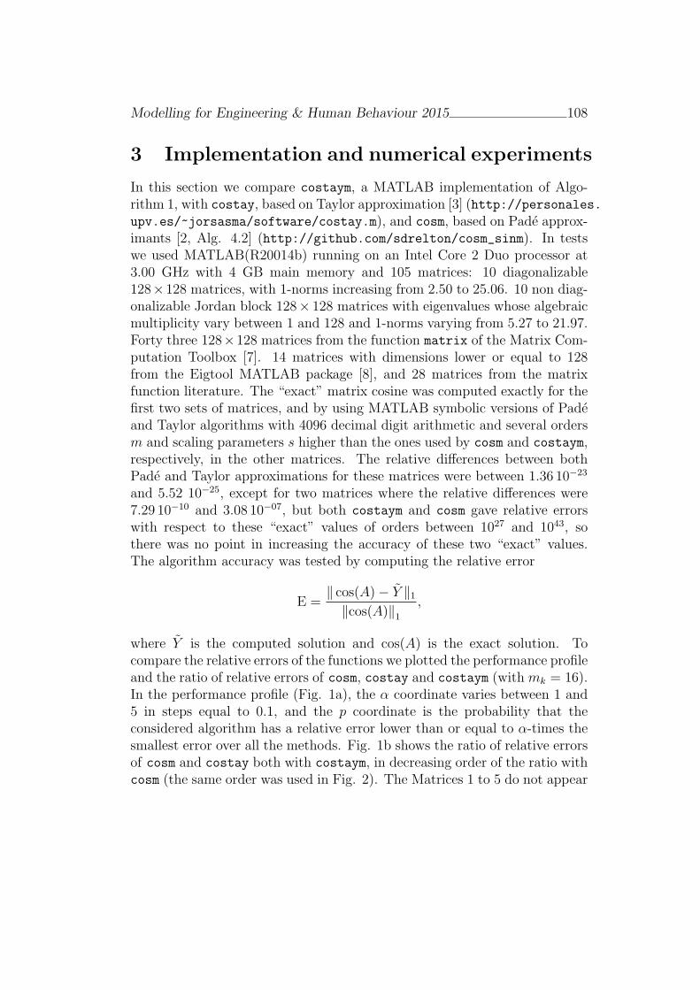
Modelling for Engineering & Human Behaviour 2015 108
3 Implementation and numerical experiments
In this section we compare costaym, a MATLAB implementation of Algo-rithm 1, with costay, based on Taylor approximation [3] (http://personales.upv.es/~jorsasma/software/costay.m), and cosm, based on Pade approx-imants [2, Alg. 4.2] (http://github.com/sdrelton/cosm_sinm). In testswe used MATLAB(R20014b) running on an Intel Core 2 Duo processor at3.00 GHz with 4 GB main memory and 105 matrices: 10 diagonalizable128×128 matrices, with 1-norms increasing from 2.50 to 25.06. 10 non diag-onalizable Jordan block 128× 128 matrices with eigenvalues whose algebraicmultiplicity vary between 1 and 128 and 1-norms varying from 5.27 to 21.97.Forty three 128×128 matrices from the function matrix of the Matrix Com-putation Toolbox [7]. 14 matrices with dimensions lower or equal to 128from the Eigtool MATLAB package [8], and 28 matrices from the matrixfunction literature. The “exact” matrix cosine was computed exactly for thefirst two sets of matrices, and by using MATLAB symbolic versions of Padeand Taylor algorithms with 4096 decimal digit arithmetic and several ordersm and scaling parameters s higher than the ones used by cosm and costaym,respectively, in the other matrices. The relative differences between bothPade and Taylor approximations for these matrices were between 1.36 10−23
and 5.52 10−25, except for two matrices where the relative differences were7.29 10−10 and 3.08 10−07, but both costaym and cosm gave relative errorswith respect to these “exact” values of orders between 1027 and 1043, sothere was no point in increasing the accuracy of these two “exact” values.The algorithm accuracy was tested by computing the relative error
E =∥ cos(A)− Y ∥1
∥cos(A)∥1,
where Y is the computed solution and cos(A) is the exact solution. Tocompare the relative errors of the functions we plotted the performance profileand the ratio of relative errors of cosm, costay and costaym (with mk = 16).In the performance profile (Fig. 1a), the α coordinate varies between 1 and5 in steps equal to 0.1, and the p coordinate is the probability that theconsidered algorithm has a relative error lower than or equal to α-times thesmallest error over all the methods. Fig. 1b shows the ratio of relative errorsof cosm and costay both with costaym, in decreasing order of the ratio withcosm (the same order was used in Fig. 2). The Matrices 1 to 5 do not appear
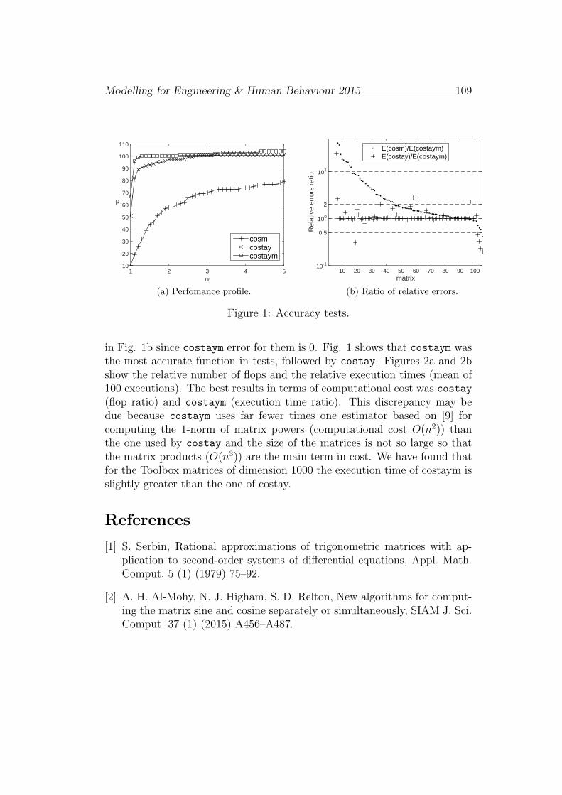
Modelling for Engineering & Human Behaviour 2015 109
α
1 2 3 4 5
p
10
20
30
40
50
60
70
80
90
100
110
cosmcostaycostaym
(a) Perfomance profile.
matrix10 20 30 40 50 60 70 80 90 100
Rel
ativ
e er
rors
rat
io
10-1
0.5
100
2
101
E(cosm)/E(costaym)E(costay)/E(costaym)
(b) Ratio of relative errors.
Figure 1: Accuracy tests.
in Fig. 1b since costaym error for them is 0. Fig. 1 shows that costaym wasthe most accurate function in tests, followed by costay. Figures 2a and 2bshow the relative number of flops and the relative execution times (mean of100 executions). The best results in terms of computational cost was costay(flop ratio) and costaym (execution time ratio). This discrepancy may bedue because costaym uses far fewer times one estimator based on [9] forcomputing the 1-norm of matrix powers (computational cost O(n2)) thanthe one used by costay and the size of the matrices is not so large so thatthe matrix products (O(n3)) are the main term in cost. We have found thatfor the Toolbox matrices of dimension 1000 the execution time of costaym isslightly greater than the one of costay.
References
[1] S. Serbin, Rational approximations of trigonometric matrices with ap-plication to second-order systems of differential equations, Appl. Math.Comput. 5 (1) (1979) 75–92.
[2] A. H. Al-Mohy, N. J. Higham, S. D. Relton, New algorithms for comput-ing the matrix sine and cosine separately or simultaneously, SIAM J. Sci.Comput. 37 (1) (2015) A456–A487.
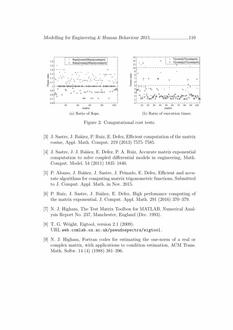
Modelling for Engineering & Human Behaviour 2015 110
matrix20 40 60 80 100
Flo
ps r
atio
0.6
0.7
0.8
0.9
1
1.1
1.2
1.3
1.4
1.5
1.6flops(cosm)/flops(costaym)flops(costay)/flops(costaym)
(a) Ratio of flops.
matrix10 20 30 40 50 60 70 80 90 100
Tim
es r
atio
0
1
2
3
4
5
6
7
8
9
10
11
12
13T(cosm)/T(costaym)T(costay)/T(costaym)
(b) Ratio of execution times.
Figure 2: Computational cost tests.
[3] J. Sastre, J. Ibanez, P. Ruiz, E. Defez, Efficient computation of the matrixcosine, Appl. Math. Comput. 219 (2013) 7575–7585.
[4] J. Sastre, J. J. Ibanez, E. Defez, P. A. Ruiz, Accurate matrix exponentialcomputation to solve coupled differential models in engineering, Math.Comput. Model. 54 (2011) 1835–1840.
[5] P. Alonso, J. Ibanez, J. Sastre, J. Peinado, E. Defez, Efficient and accu-rate algorithms for computing matrix trigonometric functions, Submittedto J. Comput. Appl. Math. in Nov. 2015.
[6] P. Ruiz, J. Sastre, J. Ibanez, E. Defez, High perfomance computing ofthe matrix exponential, J. Comput. Appl. Math. 291 (2016) 370–379.
[7] N. J. Higham, The Test Matrix Toolbox for MATLAB, Numerical Anal-ysis Report No. 237, Manchester, England (Dec. 1993).
[8] T. G. Wright, Eigtool, version 2.1 (2009).URL web.comlab.ox.ac.uk/pseudospectra/eigtool.
[9] N. J. Higham, Fortran codes for estimating the one-norm of a real orcomplex matrix, with applications to condition estimation, ACM Trans.Math. Softw. 14 (4) (1988) 381–396.

Modelling for Engineering & Human Behaviour 2015_______________________111
Modelling the spread of gender violence in Spain
Sonia Barreda1; Elena De la Poza*2; Lucas Jódar1
1 Instituto Universtario de Matemática Multidisciplinar. Universitat Politècnica de València 2 Centro de Ingeniería Económica. Departamento de Economía y Ciencias Sociales. Universitat
Politècnica de València * Corresponding author email: [email protected]
Abstract 793 (September 2015) women were assassinated by their significant other in Spain since 2003 up until now. Even when the number of gender victims is comparable to the number of victims by traffic or terrorism, the Government has not assigned equal amount of resources to reduce the magnitude of this hidden social problem. In this paper we model the spread of this social disease, dividing the Spanish male population aged among the interval [16, 70] in mutually exclusive compartments according to degrees of gender abuse. Our results show a worsening of the trend of last years. However, recommendations are given to reduce the propagation of this problem.
1. Introduction
Gender violence is an old and universal problem, happening worldwide. The problem is inversely proportional to the level of egalitarianism of the country. It is not until recent times that has been institutionally identified and condemned as a social urgency (1979). The intimate violence problem is mainly hidden, due to several reasons such as:
The low acceptance by the victims,
It takes place in the core of the couple,
It produces social shame, a feeling of emotional failure experienced by women,
The strength of a “machismo” culture combined with the common victim behaviour: to forgive and forget lower levels of violence which by itself does not solve any IPV situation, all the contrary promotes its increase.
The magnitude of the problem is such that 793 (September 4th 2015) women were assassinated by their significant other or ex-couple in Spain since 2003 up until now; but only 7.2% of the murdered women had reported their fear and previous IPV to police. Even when the number of gender victims is comparable to the number of victims by terrorism, the Government has not assigned equal amount of resources to reduce the magnitude of this hidden social problem. The primary goal of this work consist of modelling the spread of this social disease to quantify the number of intimate partner aggressors aged [16, 74] in Spain during the period 2012-2017. Also, to provide recommendations (individual and Public Authorities) to reduce and prevent the magnitude of this social epidemic.

Modelling for Engineering & Human Behaviour 2015_______________________112
2. Methods 2.1 Population of study At January 2012, male population aged [16, 74] in Spain amounted to 16,794,613 men. Then, the first step consists of splitting the population of potential men abusers in Spain aged among the interval [16, 74] in four compartments: Gender Egalitarian men; regular man; emotional-psychological abuser and physical aggressor. S: Gender Egalitarian man defined as men free of sexist micro-aggressions, (Altrocchi and Crosby, 1989) N: Regular men defined as men influenced by the general sexist environment and they may practice low intensity sexist micro-aggression. AS: Emotional-Psychological abuser, men who try to make their partners feel bad about themselves or they attack their partner’s self-esteem, (Stith, 2011). AF: Physical aggressor men who use physical force against their partner including forced sexual activity, (Stith, 2011). S(n)=1,713,051, meant to be the 30% of the male population aged [16,40] at semester n=1. Indeed the 10.20% of the total male population, MacroSurvey, Spanish Ministry of Gender Issues, 2011). N(n)= 8,901,145 represented the 53% of the total male population AS(n)= 6,046,061 represented the 36% of the total male population, (Meil, 2012). AF(n)= 134,359 amounted to the 0.8% of the total male population, (Spanish Ministry of Justice) Following we identify the drivers that lead men to transit from one subpopulation to another. By modelling the transit coefficients we can build the mathematical model that allow us to predict the number of IPV aged [16, 74] in Spain in 2017.
2.2. Transition Coefficients’ Modelling Firstly, the factors that affect the transition between subpopulations were identified as follows:
-Demographics (birth & death rate and emigration) -Women's role in the couple -Men’s alcohol and drug consumption
-Jealousy & wrong romantic stereotypes -Economic stress (Long-term unemployment) -Contagion effect (previous experiences of abuse) In fact, Demographic, Economic, Sociological and Technological factors are taken into account. Then, the transit coefficients are modelled and estimated: β1(n)= β1=egalitarian transit coefficient (egalitarian couple influence, from N subpopulation to S) β2(n)=β2= jealousy + drugs/alcohol consumption in a non-egalitarian relationship transit from N subpopulation to AS

Modelling for Engineering & Human Behaviour 2015_______________________113
β3(n)=β3 =drugs/alcohol consumption in a stable relationship transit from AS subpopulation to AF β4(n)=β4=LT unemployment consumers of drugs/alcohol in a broken relationship from AS subpopulation to AF β5(n)=β5=break up of a relationship with a non-egalitarian woman from S subpopulation to N β6(n)=β6 =recovery transit due to a new relationship and therapy from AF subpopulation to N β7(n)=β7= psychopathic rate transit from N subpopulation to AS β8(n)=β8=Technology stacking transit from N subpopulation to AS γ2(n)= recovery transit by stable egalitarian couple from AS subpopulation to N Following, it is explained how the coefficients are built.
β1(n)=β1= egalitarian transit coefficient The proportion of men aged [16,35] who are not jealous and their couple (stable relationship) is an egalitarian woman, β1=0.35*0.30*0.30= 0.03/4=0.0075.
β2(n)=β2=jealousy + drugs/alcohol consumption in a non-egalitarian relationship transit Assuming the hypothesis that amounts the 70% males suffer from jealousy, β2(n) measures the proportion of jealous men consuming drugs and/or alcohol in a stable relationship with a non-egalitarian woman. β2(n)=[1/2]*(0.7*(0.05+0,0E))*0.7=0,1225+0.035E, where E is a perturbation coefficient due to the difficulty to measure the proportion of consumers of drugs and alcohol. We assume the variation range of E is 2% centred about 5%
β3(n)=β3= drugs/alcohol abuse in a stable relationship transit. It is estimated as β3=0,105/2=0,0525. It reflects the proportion of men aggressors consumers of drugs and/or alcohol in a stable relationship,(Márkez et al, 2004)
β4(n)= Long term unemployment and consumers of drugs/alcohol abuse breaking the relationship.
It is estimated as β4(n)=[1/2]*[(0.5*0.27*0.02)+(0.5*(0.05+0.0E))]=0.026+0.025E It measures the proportion of long-term unemployed men consumers of drugs and alcohol whose relationship breaks (Márkez et al, 2004)
β5(n)= β5=break up of a relationship with a non-egalitarian woman. Estimated as β5=[1/2]*(0.7*0.174*0.5)=0.03045. It measures the proportion of men in a relationship with a non-egalitarian woman experiencing the break of the relationship, (Survey of Health and Sexual Habits & Ethology)
β6(n)=β6=recovery transit due to a new relationship and therapy Estimated as β6=[1/2]*[(0,5*0.3)+(0.5*0.7*0.005)]=0.08375. It measures the proportion of separated or divorced men engaging in a new relationship with an egalitarian woman plus the proportion of separated men engaging in a new relationship with a non-egalitarian women who attends to therapy (Stith, 1991)
β7(n)=psychopathic rate transit (Genetic). β7(n)=1%. It is the proportion of psychopathic men, (1%)=0.01. (Garrido, 2008).

Modelling for Engineering & Human Behaviour 2015_______________________114
β8(n)=β8= Technology stacking transit Built as β8=1/2*[0,5*0,7*0,5*0,7]= 0,06125. It measures the proportion of jealous men who are aged in the interval [16, 40] in a relationship with a non-egalitarian woman who uses technology as the channel for executing or exercising control aggression to their couples. (Logan et al., 2006)
γ2(n)= recovery transit by stable egalitarian couple It is measured as γ2(n)=1/2*[0.35*0.3*1]=0.0649. It represents the proportion of men aged in the interval [16,35] who starts a stable relationship (at least 1 year) with an egalitarian woman. Finally, the demographic factors are defined as follows: Incomers in the model due the male population becoming 16 years old, (INE). We assume these proportions remain constant for the short period of study. This coefficient is denoted as
i(n-32).
Those who exit the model, there are two types, the population becoming 75 years old but also deceased population between [16,74]. In both cases, we assume these amounts remain constant for the short period of study
considered. This coefficient is denoted as Di, 1£ i £ 4.
Finally, the emigration due to economic reasons (Izquierdo et al., 2015). We assume the amount of emigrants is sized according to the 2012 proportion of each subpopulation.
g1ri (n) =
113203*ri; 1£ i £ 4 n=0; 1 (2012)
131204*ri; 1£ i £ 4 n=2, 3 (2013)
49736*ri; 1£ i £ 4 n=4, 5 (2014)
0 11³ n³ 6 (2015, 2016, 2017)
ì
í
ïï
î
ïï
ü
ý
ïï
þ
ïï
where ri is the proportion of each subpopulation estimated at Jan 2012.
2.3 Model The model is expressed as follows:
Figure 1 draws the transits between subpopulations:
S(n+1) = S(n)+ b1N(n)+a1(n-32)- D1 -g1ri (n)-b5S(n)
N(n+1) = N(n)- b1N(n)+a2(n-32)- D2 -g1r 2(n)+ b5S(n)+ b6AF(n)+g2AS(n)- b2N(n)+T
AS(n+1) = AS(n)+a3(n-32)- D3 -g1r 3(n)-(b3 + b4)AS(n)-g2AS(n)+ b2N(n)-T
AF(n+1) = AF(n)+a4(n-32)- D4 -g1r 4(n)+ (b3 +b4)AS(n)-b6AF(n)
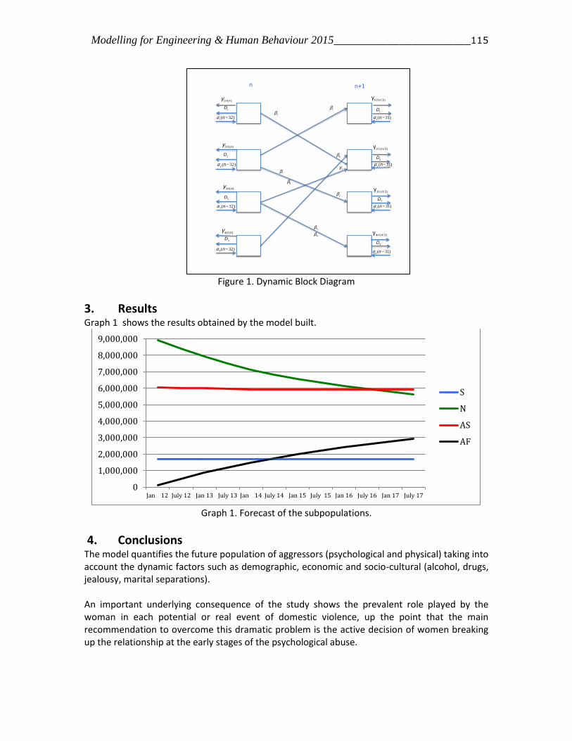
Modelling for Engineering & Human Behaviour 2015_______________________115
Figure 1. Dynamic Block Diagram
3. Results Graph 1 shows the results obtained by the model built.
Graph 1. Forecast of the subpopulations.
4. Conclusions The model quantifies the future population of aggressors (psychological and physical) taking into account the dynamic factors such as demographic, economic and socio-cultural (alcohol, drugs, jealousy, marital separations). An important underlying consequence of the study shows the prevalent role played by the woman in each potential or real event of domestic violence, up the point that the main recommendation to overcome this dramatic problem is the active decision of women breaking up the relationship at the early stages of the psychological abuse.
AF
AS
N
SS
N
AS
AF
n n+1
D1 D1
D2 D2
D3 D3
D4D4
a1(n- 32) a1(n- 31)
a2 (n- 32)
a3(n- 32)
a2 (n- 31)
a4(n- 32)a4(n- 31)
a3(n- 31)
b1
g1r i (n)
g2ri (n)
g3ri (n)
g 4ri (n)
g1r i (n+1)
g 2 r i (n+1)
g3r i (n+1)
g 4r i (n+1)
b5
g2
b2
b6
b3
b4
b7
b8
0
1,000,000
2,000,000
3,000,000
4,000,000
5,000,000
6,000,000
7,000,000
8,000,000
9,000,000
Jan 12 July 12 Jan 13 July 13 Jan 14 July 14 Jan 15 July 15 Jan 16 July 16 Jan 17 July 17
S
N
AS
AF

Modelling for Engineering & Human Behaviour 2015_______________________116
The model also surges the hidden population of aggressors that is not quantified by the official statistics, which show the problem when it is irreparable. The study is susceptible to be applied to any other geographical area where data become available as well as the period of study that can be also changed although it is important to take into account that the longer period the results obtained are less reliable.
References J. Altrocchi and R.A. Crosby, Sex Roles, June 1989, Volume 20, Issue 11-12, pp 639-648 Clarifying and measuring the concept of traditional vs. egalitarian roles in marriages MJ Diaz-Aguado; R Martinez. (2014), “Types of Adolescent Male Dating Violence Against Women, Self-Esteem, and Justification of Dominance and Aggression”.J Interpers Violence, October 17, 2014 V. Garrido, (2013), El psicópata. Algar, 2000 M. Izquierdo, J. F. Jimeno and A. Lacuesta, (2015), “Spain: From Inmigration to Emigration?”, Working paper N1503, Spanish Central Bank, Spain, Eurosystem. TK. Logan, J Cole, L Shannon. “Partner Stalking: How Women Respond, Cope, and Survive”, Springer: New York, United States, 2006.
I. Markez, C. Romera, C. Merino, X. Arana, M. Calvo, A. Peleteiro, M. Poo, (2002), Violencia
domestica, consumo de sustancias y otras circunstancias concurrentes. ¿El derecho versus
derecho a la salud? Revista de la Asociación Española Neuropsiquiatría, XXII (83), 125-133.
G. Meil, (2011), Análisis de la Encuesta sobre percepción social de la violencia de género.
Ministerio de Sanidad, Servicio Sociales e Igualdad. Delegación del Gobierno para la Violencia
de Género. C. Southworth, J. Finn, S. Dawson, C. Fraser and S. Tucker, (2007), “Intimate Partner Violence, Technology, and Stalking”, Violence Against Women, 13; 842. DOI: 10.1177/1077801207302045 Spanish Statistiscs Institute, www.ine.es S. M. Stith, E.E. McCollum, K.H.Rosen, (2011), Couples Therapy for Domestic Violence, American Psychological Association, Washington, DC.
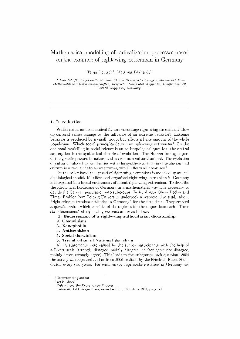
Mathematical modelling of radicalization processes based
on the example of right-wing extremism in Germany
Tanja Deutsch1, Matthias Ehrhardt1,
a Lehrstuhl für Angewandte Mathematik und Numerische Analysis, Fachbereich C
Mathematik und Naturwissenschaften, Bergische Universität Wuppertal, Gauÿstrasse 20,
42119 Wuppertal, Germany
1. Introduction
Which social and economical factors encourage right-wing extremism? Howdo cultural values change by the inuence of an extreme behavior? Extremebehavior is produced by a small group, but aects a large amount of the wholepopulation. Which social principles determine right-wing extremism? On theone hand modelling in social science is an anthropological question: the centralassumption is the synthetical theorie of evolution. The Human beeing is partof the genetic process in nature and is seen as a cultural animal. The evolutionof cultural values has similarities with the synthetical theorie of evolution andculture is a result of the same process, which aects all creatures.1
On the other hand the spread of right-wing extremism is modeled by an epi-demiological model. Manifest and organised right-wing extremism in Germanyis integrated in a broad enviroment of latent right-wing extremism. To describethe ideological landscape of Germany in a mathematical way it is necessary todevide the German population into subgroups. In April 2002 Oliver Decker andElmar Brähler from Leipzig University undertook a respresentive study about"right-wing extremism attitudes in Germany" for the rst time. They createda questionnaire, which consists of six topics with three questions each. Thesesix "dimensions" of right-wing extremism are as follows.
1. Endorsement of a right-wing authoritarian dictatorship2. Chauvinism3. Xenophobia4. Antisemitism5. Social darwinism6. Trivialisation of National SocialismAll 18 statements were valued by the survey participants with the help of
a Likert scale (strongly disagree, mainly disagree, neither agree nor disagree,mainly agree, strongly agree). This leads to ve subgroups each question. 2004the survey was repeated and as from 2006 realised by the Friedrich Ebert Foun-dation every two years. For each survey representative areas in Germany are
∗Corresponding author1see R. Boyd,
Culture and the Evolutionary Process,
University Of Chicago Press, second edition, 15th June 1988, page 1-4

Modelling for Engineering & Human Behaviour 2015 118
determined by a sample-point-selection. The subgroubs as follows are thus rep-resentive of the German society.For dening social subgroups respective the right-wing extremism in Germanywe calculate the mean value derived from the three questions each "dimension".For the years 2002 to 2014 follows for each "dimension" and each subgroup onespecic value and we obtain a classication of the German society respectiveright-wing extremism over a period of 13 years:
• G(t) Number of opponents, who disagree with the statements of therespective "dimension".
• N(t) Number of people, who have a negative attitude towards the state-ments of the respective "dimension" and mainly disagree with them.
• U(t) Number of undecided, who neither agree nor disagree with thestatements of the respective "dimension".
• S(t) Number of semi fanatics, who mainly agree with the statements ofthe respective "dimension".
• R(t) Number of radicals, who agree with the statements of the respective"dimension".
2. The ETA-model
A paper2 written by Francisco J. Santonja, Ana C. Tarazona and Rafael J.Villanueva published in 2008 describes in a mathematcial way the spread of anextreme ideology by the example of ETA in the bask country. In this modelthe size of the total population is not constant, but depends on intrinsic andextrinsic inuencing variables. There is a birth rate and mortality rate, whichhave some proportional inuence on the subgroups. Λ(t) is the number of birthsand Φ(t) the number of deaths at time t. Extrinsic the number of immigrantsΓ(t) and the number of emigrants Σ(t) inuence proportional to their sizessubgroups G and N . In this context parameters α1 and α2 describe due tosocial climate the relationship between immigration and emigration at time t.Analogous to the model built in Valencia we model the spread of right-wingextremism in Germany. The dynamics between the subgroups are described bytransition terms. It is particularly interesting how subgroup U behaves, becauseit is the fragile part of society, which is susceptible to radicalization.
After scaling the equations, we obtain the following system of ordinary dif-ferential equations.
g′(t) = (σ(t)− γ(t))g(t) + α2γ(t)− kβ1g(t)n(t)− α1σ(t), (1)
n′(t) = (σ(t)− γ(t))n(t) + (1− α2)γ(t)− β1n(t)u(t)− (1− α1)σ(t), (2)
u′(t) = (σ(t)− γ(t))u(t) + β1n(t)u(t) + β2s(t)u(t), (3)
2see F. J. Santonja, A. C. Tarazona und R. J. Villanueva,
A mathematical model of the pressure of an extreme ideology on a society,
Elsevier, August 2008
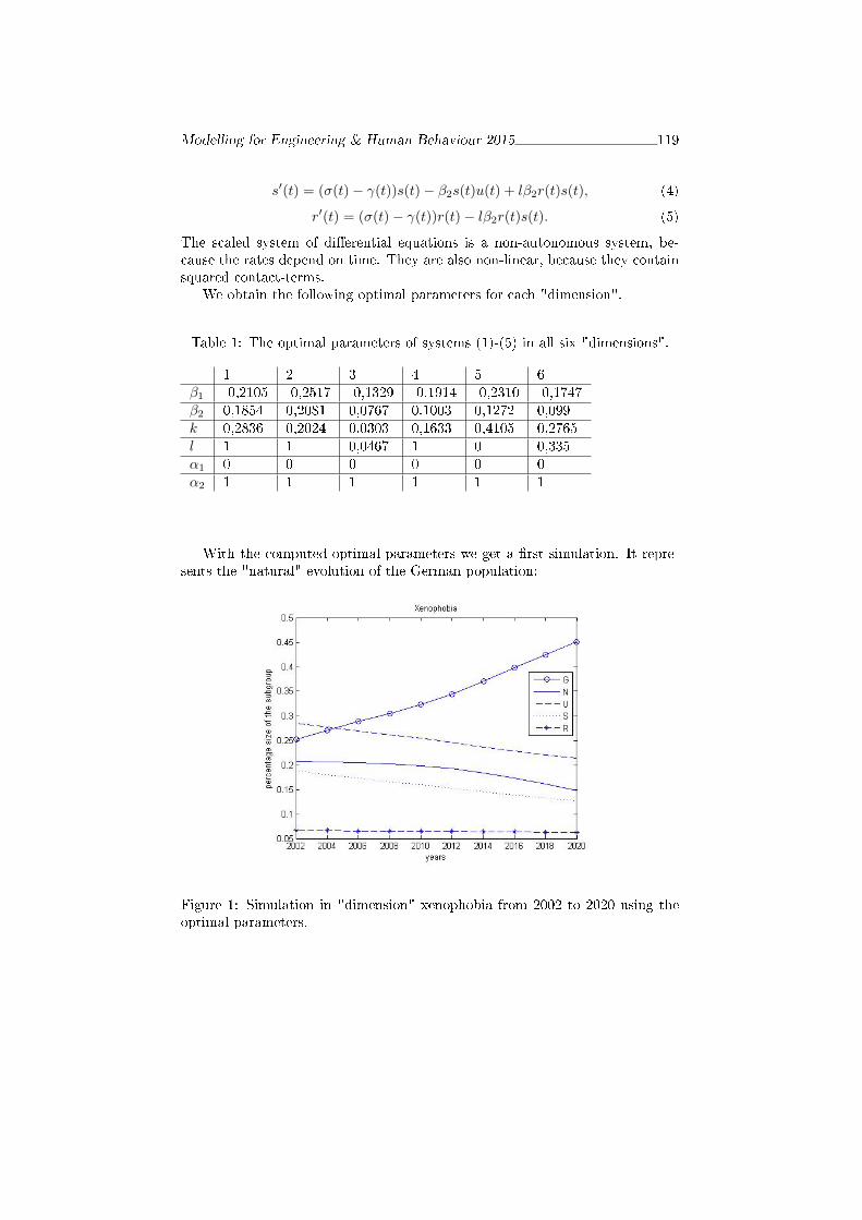
Modelling for Engineering & Human Behaviour 2015 119
s′(t) = (σ(t)− γ(t))s(t)− β2s(t)u(t) + lβ2r(t)s(t), (4)
r′(t) = (σ(t)− γ(t))r(t)− lβ2r(t)s(t). (5)
The scaled system of dierential equations is a non-autonomous system, be-cause the rates depend on time. They are also non-linear, because they containsquared contact-terms.
We obtain the following optimal parameters for each "dimension".
Table 1: The optimal parameters of systems (1)-(5) in all six "dimensions".
1 2 3 4 5 6
β1 -0,2105 -0,2517 -0,1329 -0,1914 -0,2310 -0,1747
β2 0,1854 0,2081 0,0767 0,1003 0,1272 0,099
k 0,2836 0,2024 0,0303 0,1633 0,4105 0,2765
l 1 1 0,0467 1 0 0,335
α1 0 0 0 0 0 0
α2 1 1 1 1 1 1
With the computed optimal parameters we get a rst simulation. It repre-sents the "natural" evolution of the German population:
Figure 1: Simulation in "dimension" xenophobia from 2002 to 2020 using theoptimal parameters.
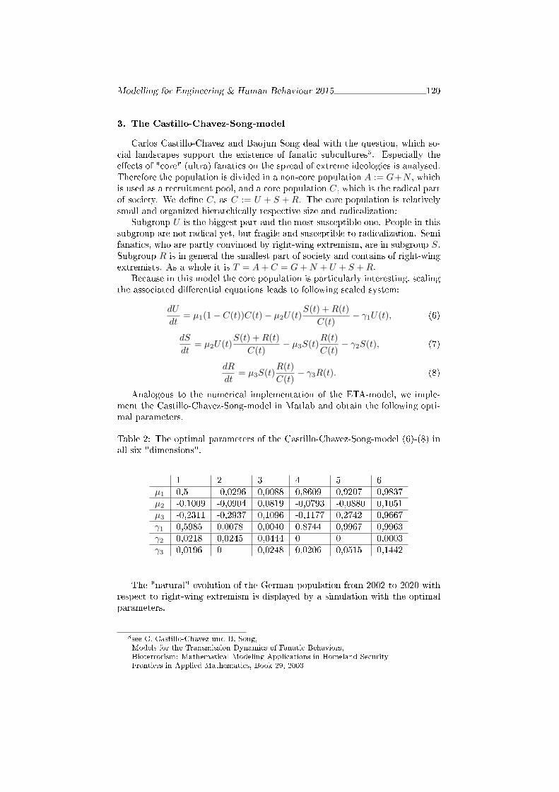
Modelling for Engineering & Human Behaviour 2015 120
3. The Castillo-Chavez-Song-model
Carlos Castillo-Chavez and Baojun Song deal with the question, which so-cial landscapes support the existence of fanatic subcultures3. Especially theeects of "core" (ultra) fanatics on the spread of extreme ideologies is analysed.Therefore the population is divided in a non-core population A := G+N , whichis used as a recruitment pool, and a core population C, which is the radical partof society. We dene C, as C := U + S + R. The core population is relativelysmall and organized hierarchically respective size and radicalization:
Subgroup U is the biggest part and the most susceptible one. People in thissubgroup are not radical yet, but fragile and susceptible to radicalization. Semifanatics, who are partly convinced by right-wing extremism, are in subgroup S.Subgroup R is in general the smallest part of society and contains of right-wingextremists. As a whole it is T = A+ C = G+N + U + S +R.
Because in this model the core population is particularly interesting, scalingthe associated dierential equations leads to following scaled system:
dU
dt= µ1(1− C(t))C(t)− µ2U(t)
S(t) +R(t)
C(t)− γ1U(t), (6)
dS
dt= µ2U(t)
S(t) +R(t)
C(t)− µ3S(t)
R(t)
C(t)− γ2S(t), (7)
dR
dt= µ3S(t)
R(t)
C(t)− γ3R(t). (8)
Analogous to the numerical implementation of the ETA-model, we imple-ment the Castillo-Chavez-Song-model in Matlab and obtain the following opti-mal parameters.
Table 2: The optimal parameters of the Castillo-Chavez-Song-model (6)-(8) inall six "dimensions".
1 2 3 4 5 6
µ1 0,5 -0,0296 0,0088 0,8609 0,9207 0,9837
µ2 -0,1009 -0,0904 0,0819 -0,0793 -0,0880 0,1051
µ3 -0,2311 -0,2937 0,1096 -0,1177 0,2742 0,9667
γ1 0,5985 0,0078 0,0040 0,8744 0,9967 0,9963
γ2 0,0218 0,0245 0,0444 0 0 0,0003
γ3 0,0196 0 0,0248 0,0206 0,0515 0,1442
The "natural" evolution of the German population from 2002 to 2020 withrespect to right-wing extremism is displayed by a simulation with the optimalparameters.
3see C. Castillo-Chavez und B. Song,
Models for the Transmission Dynamics of Fanatic Behaviors,
Bioterrorism: Mathematical Modeling Applications in Homeland Security
Frontiers in Applied Mathematics, Book 29, 2003
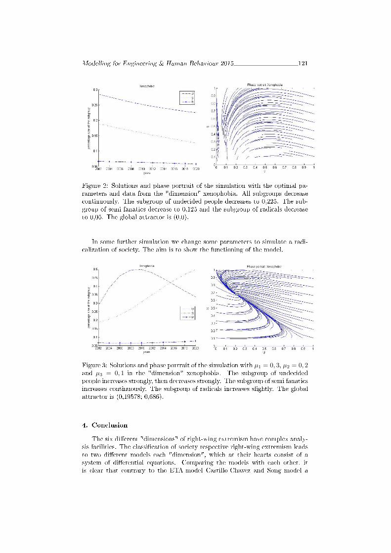
Modelling for Engineering & Human Behaviour 2015 121
Figure 2: Solutions and phase portrait of the simulation with the optimal pa-rameters and data from the "dimension" xenophobia. All subgroups decreasecontinuously. The subgroup of undecided people decreases to 0,225. The sub-group of semi fanatics decrease to 0,125 and the subgroup of radicals decreaseto 0,05. The global attractor is (0,0).
In some further simulation we change some parameters to simulate a radi-calization of society. The aim is to show the functioning of the model.
Figure 3: Solutions and phase portrait of the simulation with µ1 = 0, 3, µ2 = 0, 2and µ3 = 0, 1 in the "dimension" xenophobia. The subgroup of undecidedpeople increases strongly, then decreases strongly. The subgroup of semi fanaticsincreases continuously. The subgroup of radicals increases slightly. The globalattractor is (0,19578; 0,686).
4. Conclusion
The six dierent "dimensions" of right-wing extremism have complex analy-sis facilities. The classication of society respective right-wing extremism leadsto two dierent models each "dimension", which at their hearts consist of asystem of dierential equations. Comparing the models with each other, itis clear that contrary to the ETA-model Castillo-Chavez and Song model a
Modelling for Engineering & Human Behaviour 2015 122
circulation. Individuals, which come from a core subgroup and go via "recov-ery γi, i = 1; 2; 3, back to the moderate part of society, become part of therecruitment pool again. γ1 is in the most "dimensions" of right-wing extrem-ism the highest one, whereby a remarkable small value (γ1 = 0, 004) occurs in"dimension" xenophobia. This implies that the decimation of subgroup U issignicantly due to a transition to A. In "dimension" xenophobia subgroup Ucould be more susceptible to radicalization than to recovery. This conclusionis further suggested by µ2 = 0, 0819, which is a positive value. When γ1 isthe highest parameter, it can be derived that a radicalization is stopped afterthe transition from A to U by an early movement back to the moderate partof society. Just a few individuals become more radical. Besides xenophobia,the "dimension" chauvinism makes an exception. In this "dimensions" µ3 isaccording to amount the highest parameter. Because it is γ3 = 0 at the sametime, the decimation of subgroup R is explained by a transition from R to S.In the ETA-model the dynamics occurring are linear G ↔ N ↔ U ↔ S ↔ R,which implies a step-by-step radicalization or moderation. Explicitly a seperatimmigration and emigration rate for subgroups G and N are considered. Foreach "dimension" of right-wing extremism we get α1 = 0 and α2 = 1. Themodel gives the impression that the social climate in Germany causes an immi-gration to subgroup G and an emigration from subgroup N . The parameter lin "dimension" xenophobia is relatively small, which implies a slight dynamicR → S. In the "dimensions" endorsement of a right-wing authoriterian dic-tatorship, chauvinism and antisemitism is l = 1, which leads to equipollenttransitions U ↔ S and S ↔ R. In all "dimensions" is β1 < 0 and at thesame time β2 > 0, whereby according to amount β1 is higher than β2. This weinterpret as the central dynamic
G← N ← U ← S ← R.
Especially in "dimension" social darwinism k is relatively high, which implies astrong transition from N to G.By calculating thresholds and attractors Castillo-Chavez and Song show thatthe most eective approach for the eradication of the right-wing extremismcomes from sucient eort to limit recruitment into the radical core groupC: The control threshold is L1 = µ1
γ1. One way to bring this quantity below
1 is to reduce the value of µ1. This reduction corresponds to an increase inthe resistance of the general population A to "advances" from the core. Theelimination of the fanatic population R is critically important. L3 = µ3
γ3< 1
implies that the fanatic population will crash regardless of its size. Since thevalue of γ3 is actually a tiny number or, equivalently, since the residence time1γ3
is long, then it is quite unlikely that L3 could be made less than 1. Thisscenario leads to an increase of R.
Applying the Structural Equation Model toCo-creation in Degree Programs in Ecuadorian
Universities
Ribes-Giner, G.[ , Pantoja Dıaz, O. † ∗, and Peralt, A. ‡
([) Universidad Politecnica de Valencia,
Espana,
(†) Escuela Politecnica Nacional,
Ecuador,
(‡) European University of Valencia,
Espana,
November 30, 2015
1 Abstract
Although a number of studies have been carried out on co-creation in inno-vative marketing, only a few apply this approach to higher education. Theaim of this paper is to study the links between participation, communication,co-creation and satisfaction in undergraduate programs, in order to validatea model that could be applied in this field to enhance strategic management.In this approach the student is considered the cornerstone of the collabora-tion and a valuable stakeholder in the academic process. The literature wasreviewed for topics supporting the proposed model and Structural EquationModeling was applied to validate it. The results demonstrate that co-creationis an innovative approach that guarantees higher levels of satisfaction in theuniversity context.
∗e-mail: [email protected]
123
Modelling for Engineering & Human Behaviour 2015 124
2 Introduction
Co-creation is related to co-creation and co-production and is designed toinvolve clients as active participants in different steps of creating servicesor products. The co-creation approach has been studied by various authors[5, 9]. This tendency has been analyzed in different contexts, including in-formation technology [4], the footwear sector [15], tourism, travel services[6] and financial services [2]. In the field of higher education, [17]; [16]; and[12] focused on postgraduates programs and found co-creation had a positiveimpact and generated student loyalty.
The objective of the present study is to analyze the different relationshipsthat emerge when co-creation is applied to undergraduate students. Thisresearch was expected to allow us to validate or reject a proposed co-creationmodel, designed to be adopted as a strategic management tool in order togive universities a competitive advantage.
Adopting co-creation as a plausible alternative makes it possible to con-nect with students from the initial phase of idea generation [9]. In this way,the university obtains enhanced information on what students actually want[3] and from the students’ perspective it improves their perception, trust,satisfaction and loyalty.
The study firstly focuses on a review of the literature, in order to pro-pose a solid model based on co-creation. The principal constructs analyzedare communication, participation, co-creation and satisfaction. Exploratoryand confirmatory factor analysis and structural equation modeling were thestatistical tools implemented to validate the model, and undergraduate pro-grams were used as the case study.
3 The Conceptual Model
This section delves into the theoretical foundation of the proposed co-creationmodel, with participation, communication, co-creation and satisfaction as theprincipal constructs.
3.1 Communication vs Participation
Several studies, e.g. [1, 8] have shown the relationship between communica-tion and participation.

Modelling for Engineering & Human Behaviour 2015 125
3.2 Participation vs Co-Creation
[2] and [5] comment on the direct and positive effect of participation onco-creation.
3.3 Communication vs Co-Creation
[11, 10, 13] have shown that communication with the customer is vital forsuccessful co-creation.
3.4 Co-Creation vs Satisfaction
Satisfaction is one of the principal results of co-creation. This relationshiphas been studied by authors such as [14, 6] and [7].
3.5 The Proposed Co-creation Model
The proposed model is shown in Figure 1, and includes all the aforementionedrelationships between communication and participation, participation andco-creation, communication and co-creation and co-creation and satisfaction.
Figure 1: The Co-creation Research Model.
4 Methodology and Results
A questionnaire was given to 395 Ecuadorian undergraduate students from11 different universities, using a seven-item Likert scale.
The exploratory factor analysis was applied to validate the instrumentsused in the SPSS program. The Varimax Rotation and the Maximum Like-lihood extraction method with 4 fixed components were used to detect prob-lems and found four items in the first iteration. In the second iteration the
Modelling for Engineering & Human Behaviour 2015 126
conflicting items were excluded and a Cronbach’s alpha of about 0.906 wasobtained (over 0.7 is good). The explained variance was about 64.4%, theKMO value was 0.910 (higher than 0.5), and the Bartlett test gave p=.000.
A confirmatory factor analysis was carried out with the objective of ex-ploring the associations between items and constructs, using SPSS AMOS(Analysis of Moment Structures) program. The convergent validity wasverified, since all the constructs had an average variance extracted (AVE)above 0.5. The composite reliability of the constructs also showed valueshigher than 0.7, and the factor loadings for communication, participation,co-creation and satisfaction were higher than 0.5. The estimated coefficientsof each item were all significant (t-value > 2.0). The discriminant validitywas checked through the square roots of the AVEs, in which all the constructshad higher values than the inter-construct correlations.
The final analysis was by the commonly used structural equation model-ing (SEM), to find the relationships between the constructs. Different indica-tors were studied to determine whether the model had a good fit. The com-parative fix index (CFI) had a good value of 0.96 (over 0.95), and the adjustedgoodness-of-fit index (AGFI) also showed a good value of 0.903 (>0.8). Theroot mean square residual (RMR) was 0.076 (<0.09), the normative fit index(NFI) was 0.948 and the root mean square error of approximation (RMSEA)was 0.077 (<0.08). The squared multiple correlation of co-creation showedthat 62% (a high value) of this element is explained by the direct effect ofparticipation and the direct and indirect effects of communication. In thecase of participation, half of its variance (46%) is explained by the directimpact of communication and 68% of the satisfaction variance is explainedby the direct effect of co-creation.
Also studied was mediation by participation in the relationship betweencommunication and co-creation, where a poor but significant partial media-tion was detected.
These results led us to conclude that the four relationships studied havesignificant and positive impacts, thus proving that the four hypotheses re-lated to the undergraduate programs context were correct:
• Communication has a positive and significant impact above co-creation(γ =0.62, p-value <0.001).
• Communication has a positive and significant impact on participation(γ=0.68, p-value < 0.001).
Modelling for Engineering & Human Behaviour 2015 127
• Participation has a positive and significant effect on co-creation with alesser impact (β=0.22, p-value = 0.003).
• Co-creation has a significant and the highest impact on satisfaction(β=0.83, p-value < 0.001).
References
[1] James C Anderson and James A Narus. A model of distributor firmand manufacturer firm working partnerships. the Journal of Marketing,pages 42–58, 1990.
[2] Seigyoung Auh, Simon J Bell, Colin S McLeod, and Eric Shih. Co-production and customer loyalty in financial services. Journal of retail-ing, 83(3):359–370, 2007.
[3] Lance A Bettencourt, Stephen W Brown, and Nancy J Sirianni. Thesecret to true service innovation. Business Horizons, 56(1):13–22, 2013.
[4] Ja-Shen Chen, Hung-Tai Tsou, and Russell KH Ching. Co-productionand its effects on service innovation. Industrial Marketing Management,40(8):1331–1346, 2011.
[5] Michael Etgar. A descriptive model of the consumer co-production pro-cess. Journal of the Academy of Marketing Science, 36(1):97–108, July2007.
[6] Ursula S Grissemann and Nicola E Stokburger-Sauer. Customer co-creation of travel services: The role of company support and customersatisfaction with the co-creation performance. Tourism Management,33(6):1483–1492, 2012.
[7] Christian Gronroos. Service logic revisited: who creates value? and whoco-creates? European Business Review, 20(4):298–314, 2008.
[8] Thomas Kohler, Kurt Matzler, and Johann Fuller. Avatar-based inno-vation: Using virtual worlds for real-world innovation. Technovation,29(6):395–407, 2009.
Modelling for Engineering & Human Behaviour 2015 128
[9] Per Kristensson, Jonas Matthing, and Niklas Johansson. Key strate-gies for the successful involvement of customers in the co-creation ofnew technology-based services. International Journal of Service Indus-try Management, 19(4):474–491, 2008.
[10] Anders Lundkvist and Ali Yakhlef. Customer involvement in new servicedevelopment: a conversational approach. Managing Service Quality,14(2/3):249–257, 2004.
[11] Albert M Muniz Jr and Hope Jensen Schau. How to inspire value-laden collaborative consumer-generated content. Business Horizons,54(3):209–217, 2011.
[12] Agustın Peralt Rillo and Gabriela Ribes-Giner. Una orientacion proac-tiva hacia el mercado para los programas de Postgrado. Direccion yOrganizacion, 50:37–47, 2013.
[13] C.K. Prahalad and Venkat Ramaswamy. Co-creating unique value withcustomers. Strategy & Leadership, 32(3):4–9, January 2004.
[14] Coimbatore Krishna Prahalad and Venkat Ramaswamy. The future ofcompetition: Co-creating unique value with customers. Harvard BusinessPress, 2013.
[15] Venkat Ramaswamy. Co-creating value through customers’ experiences:the Nike case. Strategy & Leadership, 36(5):9–14, 2008.
[16] Gabriela Ribes-Giner, A. Peralt Rillo, and Ismael Moya Clemente. Co-creation innovation model for masters programs in the universities. In-novation and Teaching Technologies, 117, 2014.
[17] Gabriela Ribes-Giner and Agustın Peralt Rillo. Structural equationmodeling of co-creation and its influence on the student’s satisfactionand loyalty towards university. Journal of Computational and AppliedMathematics, 2015.
Front-fixing Transformation for RegimeSwitching Model of American Options
V.N. Egorova[ ∗, R. Company[, and L. Jodar[
([) Universitat Politecnica de Valencia,
Camino de Vera s/n, 46022 Valencia, Spain
November 30, 2015
1 Introduction
We consider the American put option on the asset St = S with strike priceE and maturity T < ∞. Let Vi(S, τ) denote the option price functions,where τ = T − t denotes the time to maturity, the asset price S and theregime αt = i. Then, Vi(S.τ), 1 ≤ i ≤ I, satisfy the following free boundaryproblem:
∂Vi∂τ
=σ2i
2S2∂
2Vi∂S2
+ riS∂Vi∂S− riVi +
∑l 6=i
qil(Vl − Vi), S > S∗i (τ), 0 < τ ≤ T,
(1)where S∗i (τ) denote optimal stopping boundaries of the option. Initial con-ditions are
Vi(S, 0) = max(E − S, 0), S∗i (0) = E, i = 1, ..., I. (2)
∗e-mail: [email protected]
129
Modelling for Engineering & Human Behaviour 2015 130
Boundary conditions for i = 1, .., I are as follows
limS→∞
Vi(S, τ) = 0, (3)
Vi(S∗i (τ), τ) = E − S∗i (τ), (4)
∂Vi∂S
(S∗i (τ), τ) = −1. (5)
2 Front-Fixing transformation
Based on the transformation used by the authors in [4], [1] for the case ofjust one equation, let us consider the multivariable transformation
xi = lnS
S∗i (τ), 1 ≤ i ≤ I. (6)
Note that the new variables xi lie in the fixed positive real line. Price Viof i-th regime involved in i-th equation of the system and i-th free boundaryare related by the dimensionless transformation
Pi(xi, τ) =
Vi(S, τ)
E, Xi(τ) =
S∗i (τ)
E, 1 ≤ i ≤ I. (7)
Value of option l-th regime appearing in i-th coupled equation, l 6= i,becomes
Pl,i(xi, τ) =
Vl(S, τ)
E. (8)
Since from (7), Vl(S,τ)E
= Pl(xl, τ) and taking into account transformation
(6) for indexes i and l one gets that
Pl,i(xi, τ) = Pl(x
l, τ), (9)
and it occurs when the variables are related by the equation
xl = xi + lnXi(τ)
Xl(τ), 1 ≤ i, l ≤ I. (10)
From (6) - (9) the problem (1) - (5) for 1 ≤ i ≤ I takes a new form:
∂Pi∂τ
(xi, τ) =σ2i
2
∂2Pi∂(xi)2
(xi, τ) +
(ri −
σ2i
2+X ′i(τ)
Xi(τ)
)∂Pi∂xi
(xi, τ)
−riPi(xi, τ) +∑l 6=i
qil(Pl,i(xi, τ)− Pi(xi, τ)) = 0, xi > 0, 0 < τ ≤ T,
(11)
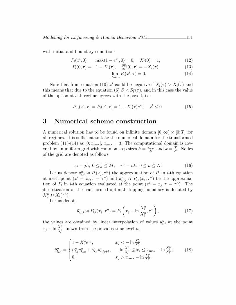
Modelling for Engineering & Human Behaviour 2015 131
with initial and boundary conditions
Pi(xi, 0) = max(1− exi , 0) = 0, Xi(0) = 1, (12)
Pi(0, τ) = 1−Xi(τ), ∂Pi
∂xi(0, τ) = −Xi(τ), (13)
limxi→∞
Pi(xi, τ) = 0. (14)
Note that from equation (10) xl could be negative if Xl(τ) > Xi(τ) andthis means that due to the equation (6) S < S∗l (τ), and in this case the valueof the option at l-th regime agrees with the payoff, i.e.
Pl,i(xi, τ) = Pl(x
l, τ) = 1−Xl(τ)exl
, xl ≤ 0. (15)
3 Numerical scheme construction
A numerical solution has to be found on infinite domain [0;∞) × [0;T ] forall regimes. It is sufficient to take the numerical domain for the transformedproblem (11)-(14) as [0;xmax], xmax = 3. The computational domain is cov-ered by an uniform grid with common step sizes h = xmax
Mand k = T
N. Nodes
of the grid are denoted as follows
xj = jh, 0 ≤ j ≤M ; τn = nk, 0 ≤ n ≤ N. (16)
Let us denote uni,j ≈ Pi(xj, τn) the approximation of Pi in i-th equation
at mesh point (xi = xj, τ = τn) and unli,j ≈ Pl,i(xj, τn) be the approxima-
tion of Pl in i-th equation evaluated at the point (xi = xj, τ = τn). Thediscretization of the transformed optimal stopping boundary is denoted byXni ≈ Xi(τ
n).Let us denote
unli,j ≈ Pl,i(xj, τn) = Pl
(xj + ln
Xni
Xnl
, τn), (17)
the values are obtained by linear interpolation of values unl,j at the point
xj + lnXn
i
Xnl
known from the previous time level n,
unli,j =
1−Xn
i exj , xj < − ln
Xni
Xnl
;
αnl,junl,j0
+ βnl,junl,j0+1, − ln
Xni
Xnl≤ xj ≤ xmax − ln
Xni
Xnl
;
0, xj > xmax − lnXn
i
Xnl.
(18)
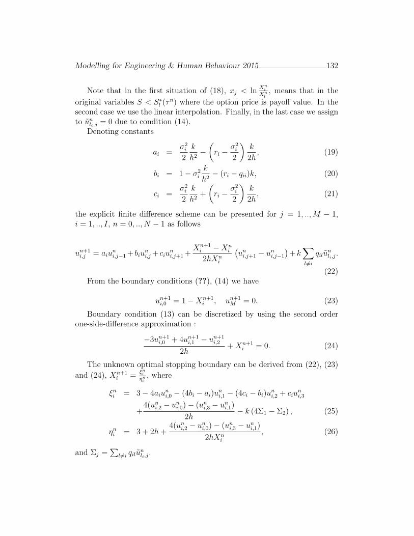
Modelling for Engineering & Human Behaviour 2015 132
Note that in the first situation of (18), xj < lnXn
i
Xnl
, means that in the
original variables S < S∗l (τn) where the option price is payoff value. In the
second case we use the linear interpolation. Finally, in the last case we assignto unli,j = 0 due to condition (14).
Denoting constants
ai =σ2i
2
k
h2−(ri −
σ2i
2
)k
2h, (19)
bi = 1− σ2i
k
h2− (ri − qii)k, (20)
ci =σ2i
2
k
h2+
(ri −
σ2i
2
)k
2h, (21)
the explicit finite difference scheme can be presented for j = 1, ..,M − 1,i = 1, .., I, n = 0, .., N − 1 as follows
un+1i,j = aiu
ni,j−1 + biu
ni,j + ciu
ni,j+1 +
Xn+1i −Xn
i
2hXni
(uni,j+1 − uni,j−1
)+k
∑l 6=i
qilunli,j.
(22)From the boundary conditions (??), (14) we have
un+1i,0 = 1−Xn+1
i , un+1M = 0. (23)
Boundary condition (13) can be discretized by using the second orderone-side-difference approximation :
−3un+1i,0 + 4un+1
i,1 − un+1i,2
2h+Xn+1
i = 0. (24)
The unknown optimal stopping boundary can be derived from (22), (23)
and (24), Xn+1i =
ξniηni, where
ξni = 3− 4aiuni,0 − (4bi − ai)uni,1 − (4ci − bi)uni,2 + ciu
ni,3
+4(uni,2 − uni,0)− (uni,3 − uni,1)
2h− k (4Σ1 − Σ2) , (25)
ηni = 3 + 2h+4(uni,2 − uni,0)− (uni,3 − uni,1)
2hXni
, (26)
and Σj =∑
l 6=i qilunli,j
.
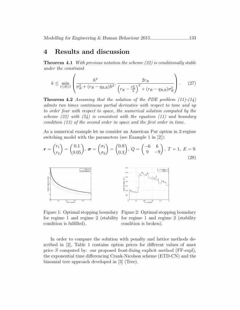
Modelling for Engineering & Human Behaviour 2015 133
4 Results and discussion
Theorem 4.1 With previous notation the scheme (22) is conditionally stableunder the constraint
k ≤ min1≤R≤I
h2
σ2R + (rR − qR,R)h2
,2rR(
rR −σ2R
2
)2+ (rR − qR,R)σ2
R
. (27)
Theorem 4.2 Assuming that the solution of the PDE problem (11)-(14)admits two times continuous partial derivative with respect to time and upto order four with respect to space, the numerical solution computed by thescheme (22) with (24) is consistent with the equation (11) and boundarycondition (13) of the second order in space and the first order in time.
As a numerical example let us consider an American Put option in 2-regimeswitching model with the parameters (see Example 1 in [2]):
r =
(r1r2
)=
(0.1
0.05
), σ =
(σ1σ2
)=
(0.8
0.3
), Q =
(−6 69 −9
), T = 1, E = 9.
(28)
0 0.2 0.4 0.6 0.8 13
4
5
6
7
8
9
Time to maturity
Opt
imal
sto
ppin
g bo
unda
ry
Regime 1Regime 2
Figure 1: Optimal stopping boundaryfor regime 1 and regime 2 (stabilitycondition is fulfilled).
Figure 2: Optimal stopping boundaryfor regime 1 and regime 2 (stabilitycondition is broken).
In order to compare the solution with penalty and lattice methods de-scribed in [2], Table 1 contains option prices for different values of assetprice S computed by: our proposed front-fixing explicit method (FF-expl),the exponential time differencing Crank-Nicolson scheme (ETD-CN) and thebinomial tree approach developed in [3] (Tree).
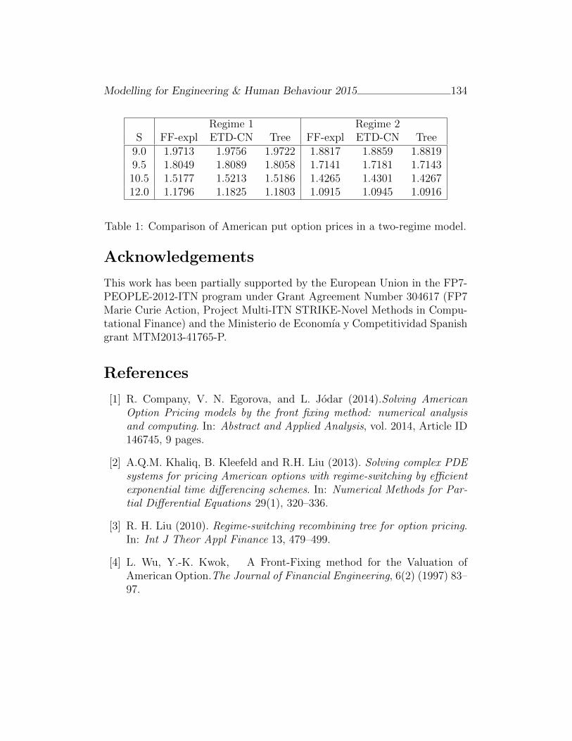
Modelling for Engineering & Human Behaviour 2015 134
Regime 1 Regime 2S FF-expl ETD-CN Tree FF-expl ETD-CN Tree
9.0 1.9713 1.9756 1.9722 1.8817 1.8859 1.88199.5 1.8049 1.8089 1.8058 1.7141 1.7181 1.714310.5 1.5177 1.5213 1.5186 1.4265 1.4301 1.426712.0 1.1796 1.1825 1.1803 1.0915 1.0945 1.0916
Table 1: Comparison of American put option prices in a two-regime model.
Acknowledgements
This work has been partially supported by the European Union in the FP7-PEOPLE-2012-ITN program under Grant Agreement Number 304617 (FP7Marie Curie Action, Project Multi-ITN STRIKE-Novel Methods in Compu-tational Finance) and the Ministerio de Economıa y Competitividad Spanishgrant MTM2013-41765-P.
References
[1] R. Company, V. N. Egorova, and L. Jodar (2014).Solving AmericanOption Pricing models by the front fixing method: numerical analysisand computing. In: Abstract and Applied Analysis, vol. 2014, Article ID146745, 9 pages.
[2] A.Q.M. Khaliq, B. Kleefeld and R.H. Liu (2013). Solving complex PDEsystems for pricing American options with regime-switching by efficientexponential time differencing schemes. In: Numerical Methods for Par-tial Differential Equations 29(1), 320–336.
[3] R. H. Liu (2010). Regime-switching recombining tree for option pricing.In: Int J Theor Appl Finance 13, 479–499.
[4] L. Wu, Y.-K. Kwok, A Front-Fixing method for the Valuation ofAmerican Option.The Journal of Financial Engineering, 6(2) (1997) 83–97.
Positive numerical solution of two assetjump-diffusion partial-integro differential
models
M. Fakharany[ ∗, R. Company[, and L. Jodar[
([) Instituto de Matematica Multidisciplinar, Universitat Politecnica de Valencia,
Camino de Vera s/n, 46022 Valencia, Spain.
November 30, 2015
1 Introduction
In this paper a finite difference scheme for the partial-integro differentialequation (PIDE) for two assets under jump-diffusion model is proposed.First, in order to avoid numerical drawbacks of the mixed derivative term, asuitable transformation of variables removes this term. Second, the centralfinite difference approximation in space is implemented for the differentialpart of the new PIDE, while the integral part is approximated using a 2DGauss-Hermite quadrature reducing the computational cost.The stochastic differential equations for a two-dimensional Merton jump dif-fusion model are given by
dSi(t)
Si(t)= (r − qi − λκi)dt+ σidWi + (eJi − 1)dZ(t), i = 1, 2, (1)
where Si, qi, σi, i = 1, 2 are the two assets prices, asset dividend yields,asset volatilities respectively, r is the risk free interest and Wi are standardBrownian motions correlated by ρ ∈ (−1, 1). J1 and J2 are the jump sizescorrelated by ρJ ∈ (−1, 1), κi represent the expected relative jump sizes
∗e-mail: [email protected]
135
Modelling for Engineering & Human Behaviour 2015 136
(κi = E[eJi − 1]), Z and λ are the poisson process and its jump intensity.Based on Ito calculus, the corresponding PIDE for the unknown option priceU(x1, x2, τ) takes the form
∂U
∂τ=σ21
2
∂2U
∂x21+ ρσ1σ2
∂2U
∂x1∂x2+σ22
2
∂2U
∂x22+
(r − q1 − λκ1 −
σ21
2
)∂U
∂x1
+
(r − q2 − λκ2 −
σ22
2
)∂U
∂x2−(r+λ)U+λ
∫R2
U(x1+η1, x2+η2)g(η1, η2)dη1dη2,
(2)where (x1, x2) = (lnS1/E, lnS2/E), E is the strike price, τ = T − t is thetime to maturity and g(η1, η2) is the probability density function of a bivariatenormal distribution, given by
g(η1, η2) =
exp
[− 1
2(1−ρ2J )
((η1−µ1σ1
)2− 2ρJ (η1−µ1)(η2−µ2)
σ1σ2+(η2−µ2σ2
)2)]2πσ1σ2
√1− ρ2J
, (3)
such that µ1, µ2, σ1 and σ2 are the means and standard deviations of thejumps J1 and J2 respectively. There are several kinds of two assets problemdepending on the nature of the payoff. Here we focus on options of the bestand worst types. In this case, the option gives a holder the right to receivethe maximum or minimum of the two underlying assets at maturity. Thepayoff f(x1, x2) for put on minimum [1, 3] and the boundary conditions aregiven by
f(x1, x2) = Emax(1−min(ex1 , ex2), 0) (4)
limx1→−∞ U(x1, x2, τ) = Ee−rτ , limx2→−∞ U(x1, x2, τ) = Ee−rτ ,limx1→∞ ∂x1U(x1, x2, τ) = 0, limx2→∞ ∂x2U(x1, x2, τ) = 0.
(5)
2 The problem transformation and numerical
scheme
From numerical analysis view, the presence of the mixed derivative in thePIDE leads to several problems in the numerical scheme performance suchas delaying the convergence and poor accuracy. Moreover, the discretizationof this term requires nine or seven constrained stencil points which increasesthe computational cost. Here this term is removed using the characteristic
Modelling for Engineering & Human Behaviour 2015 137
equation as in [4, 5] since ∆ = σ21σ
22(ρ2−1) < 0. Consequently, the PIDE (2)
is of elliptic type, then by using the canonical transformation [6], the suitablechange or variables are given by
y1 =σ2ρ
σ1x1, y2 = x2−
σ2ρ
σ1x1 = x2−my1, m =
ρ
ρ, V (y1, y2, τ) = exp((r+λ)τ)U(x1, x2, τ),
(6)and (2) is transformed into
∂V∂τ
=σ22 ρ
2
2
(∂2V∂y21
+ ∂2V∂y22
)+ a1
∂V∂y1
+ a2∂V∂y2
+σ1λσ2ρ
∫R2 V (φ1, φ2, τ)g( σ1
σ2ρ(φ1 − y1), φ2 − y2 + m(φ1 − y1))dφ1dφ2,
(7)
where
a1 = ρσ2σ1
(r − q1 − λk1 − σ21
2),
a2 =(
(1− ρσ2σ1
)r − (q2 − ρσ2σ1q1)− λκ2 + ρσ2
σ1λκ1 − σ2
2
2+ ρσ1σ2
2
),
φ1 = y1 + σ2ρσ1η1, φ2 = y2 − σ2ρ
σ1η1 + η2.
(8)
For the associated boundary conditions for Put option on minimum, one gets
limy1→−∞ V (y1, y2, τ) = Eeλτ , limy2→−∞ V (y1, y2, τ) = Eeλτ
limy1→∞ ∂y1V (y1, y2, τ) = 0, limy2→∞ ∂y2V (y1, y2, τ) = 0.(9)
Now we ready to set up an efficient explicit numerical scheme for the prob-lem (7)-(9). First, let us consider a rectangular domain in x1x2−plane withboundaries x1 ∈ [a, b] and x2 ∈ [c, d]. Under the transformation (6), the rect-angular domain is converted to a rhomboid domain in y1y2−plane. Let N1
and N2 represent the number of the discretization points in y1 and y2 direc-tions, hx1 = (b−a)/N1 and hx2 = (d−c)/N2 are the stepsizes in x1x2−plane,h1 and h2 are the stepsizes in y1y2−plane which are obtained by hx1 andhx2 such that h1 = σ2
σ1ρhx1 , h2 = hx2 . Hence y1,i = y1,0 + ih1, 0 ≤ i ≤ N1,
y1,0 = σ2σ1ρa, we discretize y2 using two indices i and j; yi2,j = yi,0 + jh2
where yi,0 = c − σ2σ1ρ(a + ihx1), 0 ≤ i ≤ N1, since we have oblique lines
and τn = nk, 0 ≤ n ≤ Nτ , k = T/Nτ . Let V ni,j be the approximation of
V (y1,i, yi2,j, τ
n), the central finite difference approximations are used for thefirst and second spatial derivatives while the explicit forward discretizationis implemented to approximate the first time-derivative of V . Finally, theintegral part is approximated using 2D Gauss-Hermite quadrature formula
Modelling for Engineering & Human Behaviour 2015 138
[7], then the corresponding finite difference scheme is given by
V n+1i,j = α1V
ni,j + α2V
ni+1,j + α3V
ni−1,j + α4V
ni,j+1 + α5V
ni,j−1 +
kλσ1σ2ρ
Ini,j, (10)
where
α1 = 1− kσ22 ρ
2( 1h21
+ 1h22
), α2 = k2h1
(σ22 ρ
2
h1+ a1), α3 = k
2h1(σ22 ρ
2
h1− a1),
α4 = k2h2
(σ22 ρ
2
h2+ a2), α5 = k
2h2(σ22 ρ
2
h2− a2),
(11)
Ini,j =L∑`=1
M∑m=1
ω`ωmg(σ1σ2ρ
(φ1,`−y1,i), φ2,m−yi2,j+m(φ1,`−y1,i)) exp[φ21,`+φ
22,m]V n(φ1,`, φ2,m),
(12)such that φm and φ` are the roots of Hermite polynomials of degrees M andL respectively. ωm and ω` are the corresponding weighting values.Since (φ1,`, φ2,m) are not necessary points of the grid, then in order to matchthe discretization of the integral part with the differential part, the bivariateinterpolation four point approximation [7] is used. Hence the approximationfor V n
`,m is given by
V n`,m ≈ δi`,2(δjm,2V
ni`,jm
+ δjm,1Vni`,jm+1) + δi`,1(δjm,3V
ni`+1,jm+1 + δjm,4V
ni`+1,jm),
(13)where
δi`,1 =φ1,`−y1,i`
h1, δi`,2 =
y1,i`+1−φ1,`h1
, δjm,1 =φ2,m−y
i`2,jm
h2,
δjm,2 =yi`2,jm+1−φ2,m
h2, δjm,3 =
φ2,m−yi`+1
2,jm
h2, δjm,4 =
yi`+1
2,jm+1−φ2,mh2
.
Finally the discretization for initial and boundary conditions are
V 0i,j = f(y1,i, y
i2,j), 0 ≤ i ≤ N1, 0 ≤ j ≤ N2,
V n0,j = V n
i,0 = Eeλτn, 0 ≤ i ≤ N1, 0 ≤ j ≤ N2, n ≥ 1,
V nN1,j+1 = V n
N1,j, 0 ≤ j ≤ N2 − 1, V n
i+1,N2= V n
i,N2, 0 ≤ i ≤ N1 − 1.
3 Example
In order to show the efficiency of the proposed scheme let us consider thean European put option with parameters T = 1, E = 100, r = 0.05,q1 = q2 = 0, σ1 = 0.12, σ2 = 0.15, ρ = 0.3, λ = 0.6, µ1 = −0.1,
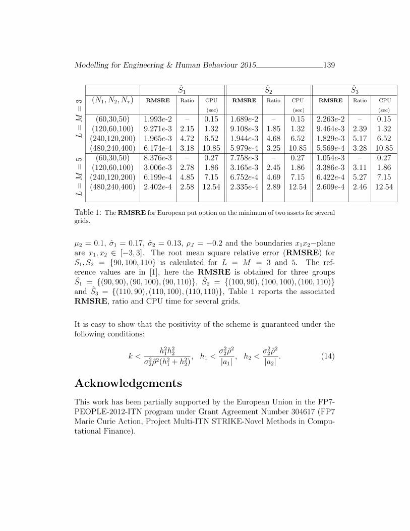
Modelling for Engineering & Human Behaviour 2015 139
S1 S2 S3
(N1, N2, Nτ ) RMSRE Ratio CPU RMSRE Ratio CPU RMSRE Ratio CPU
(sec) (sec) (sec)
(60,30,50) 1.993e-2 – 0.15 1.689e-2 – 0.15 2.263e-2 – 0.15(120,60,100) 9.271e-3 2.15 1.32 9.108e-3 1.85 1.32 9.464e-3 2.39 1.32
L=M
=3
(240,120,200) 1.965e-3 4.72 6.52 1.944e-3 4.68 6.52 1.829e-3 5.17 6.52(480,240,400) 6.174e-4 3.18 10.85 5.979e-4 3.25 10.85 5.569e-4 3.28 10.85
(60,30,50) 8.376e-3 – 0.27 7.758e-3 – 0.27 1.054e-3 – 0.27(120,60,100) 3.006e-3 2.78 1.86 3.165e-3 2.45 1.86 3.386e-3 3.11 1.86(240,120,200) 6.199e-4 4.85 7.15 6.752e-4 4.69 7.15 6.422e-4 5.27 7.15(480,240,400) 2.402e-4 2.58 12.54 2.335e-4 2.89 12.54 2.609e-4 2.46 12.54
L=M
=5
Table 1: The RMSRE for European put option on the minimum of two assets for severalgrids.
µ2 = 0.1, σ1 = 0.17, σ2 = 0.13, ρJ = −0.2 and the boundaries x1x2−planeare x1, x2 ∈ [−3, 3]. The root mean square relative error (RMSRE) forS1, S2 = 90, 100, 110 is calculated for L = M = 3 and 5. The ref-erence values are in [1], here the RMSRE is obtained for three groupsS1 = (90, 90), (90, 100), (90, 110), S2 = (100, 90), (100, 100), (100, 110)and S3 = (110, 90), (110, 100), (110, 110), Table 1 reports the associatedRMSRE, ratio and CPU time for several grids.
It is easy to show that the positivity of the scheme is guaranteed under thefollowing conditions:
k <h21h
22
σ22 ρ
2(h21 + h22), h1 <
σ22 ρ
2
|a1|, h2 <
σ22 ρ
2
|a2|. (14)
Acknowledgements
This work has been partially supported by the European Union in the FP7-PEOPLE-2012-ITN program under Grant Agreement Number 304617 (FP7Marie Curie Action, Project Multi-ITN STRIKE-Novel Methods in Compu-tational Finance).
Modelling for Engineering & Human Behaviour 2015 140
References
[1] Clift S. S., and Forsyth P. A. Numerical solution of two asset jump dif-fusion models for option valuation Applied Mathematical Mathematics,Volume(58): 743–782, 2008.
[2] Rambeerich N., Tangman D. Y., Lollchund M.R., and Bhuruth M. High-order computational methods for option valuation under multifactormodels European Journal of Operational Research, Volume(224): 219–226,2013.
[3] D. J. Duffy, Finite Difference Methods in Financial Engineering: aPartial Differential Approach. England, John Wiley & Sons Ltd, TheAtrium, Southern Gate, Chichester, West Sussex PO19 8SQ, 2006.
[4] Company R., Jodar L., Fakharany M., and Casaban M.-C. Removing thecorrelation term in the option pricing Heston model: numerical analysisand computing Abstract and Applied Analysis, Volume (2013): 1–11.
[5] Fakharany M., Company R., and Jodar L. Positive finite differenceschemes for partial integro-differential option pricing model AppliedMathematics and Computation, Volume(249): 320–332.
[6] S. J. Farlow, Partial differential equations for scientists and engineers.New York, Dover Publications Inc., 1993.
[7] M. Abramowitz and I. A. Stegun. Handbook of mathematical functions:with formulas, graphs, and mathematical tables. Dover Books on Math-ematics, 1961.
Factors Affecting the Choice Modal ofTransportation in an Urban Environment.
Hierarchical Multi-Criteria Analysis
A. Fraile[ ∗, J.A. Sicilia §, E. Larrode[ and B. Royo†
([) Department of Mechanical Engineering, Universidad de Zaragoza, Spain.
(§) Universidad Internacional de La Rioja (UNIR), Logrono, La Rioja, Spain.
(†) Instituto Tecnologico de Aragon, Zaragoza, Spain.
November 30, 2015
1 Introduction
In recent decades there have been profound social, economic and technolog-ical changes have led to a new model of urban mobility. That model, whichtends to be implemented globally, is characterized by the increase in averagedistances travelled, changes in the grounds for the displacements and changesin the location of production activities. In modern economies is essential thatsuitable transport that enables the population mobility and the consequentaccessibility to services. However, its current configuration is causing strongnegative externalities and generates much of the problems of environmental,social and energy sustainability. The changes required by the current un-sustainable configuration should be based on a new vision of transportationand the development of theoretical and empirical criteria that enable thecreation of sustainable transport systems. Such a system must be based onthe principle of multimodal transport.
The purpose of this paper is to analyze the most important factors ofurban mobility in its current configuration, analyze the negative externalities
∗e-mail: [email protected]; [email protected]
141
Modelling for Engineering & Human Behaviour 2015 142
caused by the transportation, and develop the principles necessary to developa model in which the modal distribution is optimized in a city in a way thatis sustainable, both in terms of passengers and freight.
Previously, in other works as [2, 3, 4] using different methodologies, thefactors affecting modal choice in different countries are analyzed, success sto-ries in sustainable mobility are described and traffic optimization indicatorsare described.
To do this, in the Decision Theory, it has been selected Analytic HierarchyProcess (AHP) technique to support different stages of the proposed method-ology. This technique allows by building a hierarchical model, efficiently andgraphically, organizes information about a problem, break it down and ana-lyze it by parts in different matrix, visualize the effects of changes in levelsand synthesize.
2 Objectives
The main objectives sought in this article are:
• Analyze key factors of urban mobility in the current situation of cities,taking into account all the elements involved in mobility in urban envi-ronments (technological advances, new regulations, influence the eco-nomic attitude, changes in urban planning,...) and study their behav-ior.
• From here, develop the principles necessary to develop a model to aiddecision-making for action, in order to meet three overall objectives,customer satisfaction, sustainable growth and energy and environmen-tal efficiency.
Similarly, secondary objectives are:
• Develop a model of analysis to study mobility in an urban environmenttaking into account the influence of factors affecting transport for bestmodal split.
• Justify, within the theory of decision, the selection of AHP techniqueto support various stages of the proposed methodology; Building theanalysis model, in collaboration with a group of experts in the field;Define all elements of the model (criteria, sub-criteria, attributes and
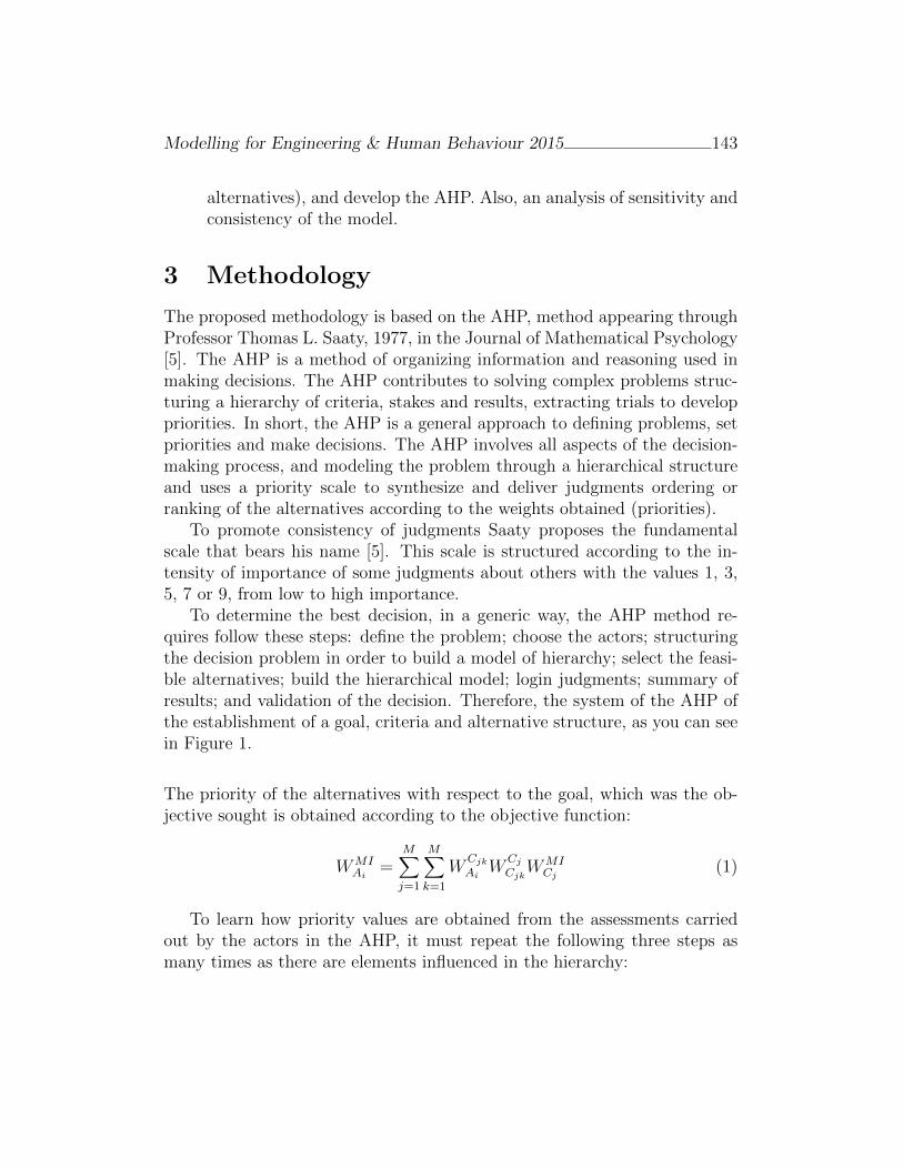
Modelling for Engineering & Human Behaviour 2015 143
alternatives), and develop the AHP. Also, an analysis of sensitivity andconsistency of the model.
3 Methodology
The proposed methodology is based on the AHP, method appearing throughProfessor Thomas L. Saaty, 1977, in the Journal of Mathematical Psychology[5]. The AHP is a method of organizing information and reasoning used inmaking decisions. The AHP contributes to solving complex problems struc-turing a hierarchy of criteria, stakes and results, extracting trials to developpriorities. In short, the AHP is a general approach to defining problems, setpriorities and make decisions. The AHP involves all aspects of the decision-making process, and modeling the problem through a hierarchical structureand uses a priority scale to synthesize and deliver judgments ordering orranking of the alternatives according to the weights obtained (priorities).
To promote consistency of judgments Saaty proposes the fundamentalscale that bears his name [5]. This scale is structured according to the in-tensity of importance of some judgments about others with the values 1, 3,5, 7 or 9, from low to high importance.
To determine the best decision, in a generic way, the AHP method re-quires follow these steps: define the problem; choose the actors; structuringthe decision problem in order to build a model of hierarchy; select the feasi-ble alternatives; build the hierarchical model; login judgments; summary ofresults; and validation of the decision. Therefore, the system of the AHP ofthe establishment of a goal, criteria and alternative structure, as you can seein Figure 1.
The priority of the alternatives with respect to the goal, which was the ob-jective sought is obtained according to the objective function:
WMIAi
=M∑j=1
M∑k=1
WCjk
AiW
Cj
CjkWMI
Cj(1)
To learn how priority values are obtained from the assessments carriedout by the actors in the AHP, it must repeat the following three steps asmany times as there are elements influenced in the hierarchy:
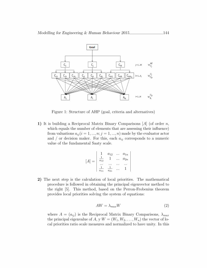
Modelling for Engineering & Human Behaviour 2015 144
Figure 1: Structure of AHP (goal, criteria and alternatives)
1) It is building a Reciprocal Matrix Binary Comparisons [A] (of order n,which equals the number of elements that are assessing their influence)from valuations aij(i = 1, ..., n; j = 1, ..., n) made by the evaluator actorand / or decision maker. For this, each aij corresponds to a numericvalue of the fundamental Saaty scale.
[A] =
∣∣∣∣∣∣∣∣∣∣1 a12 ... a1n1
a121 ... a2n
... ... ... ...1
a1n1
a2n... 1
∣∣∣∣∣∣∣∣∣∣2) The next step is the calculation of local priorities. The mathematical
procedure is followed in obtaining the principal eigenvector method tothe right [5]. This method, based on the Perron-Frobenius theoremprovides local priorities solving the system of equations:
AW = λmaxW (2)
where A = (aij) is the Reciprocal Matrix Binary Comparisons, λmax
the principal eigenvalue of A, y W = (W1,W2, . . . ,Wn) the vector of lo-cal priorities ratio scale measures and normalized to have unity. In this

Modelling for Engineering & Human Behaviour 2015 145
case, normalization has applied the so called distributive (∑
j Wj = 1).In practice, the solution W is obtained (power method) by raising thematrix judgments on a sufficiently large power, adding rows and nor-malizing these values by dividing the sum of each row for the totalamount. The process ends when the difference between two consec-utive powers is small. The priority vector w represents the relativeimportance of the criteria or sub compared in each pairwise compari-son matrices.
3) For the analysis of consistency, it is estimated the maximum eigenvalueassociated λmax with [A] and the consistency index (CI) is obtained:
CI =λmax − nn− 1
(3)
where n is the orden of the matrix.
If the reason for inconsistency (CR), where the random index (RI) isobtained from Table 1, is less than 10% then states that the valuationsare consistent and the values Wi(i = 1, ..., n) of the eigenvector Ware accepted as good. If not, the decision maker is asked to redo thevaluations of the Reciprocal Matrix Binary Comparisons:
CR =CI
RI(4)
Matrix size 1 2 3 4 5 6 7 8 9 10RI 0 0 0.525 0.882 1.115 1.252 1.341 1.404 1.452 1.484
Table 1: Table of random values (Saaty) [1]
Finally in this paper, the AHP model structure is composed of the goal, 2criterias (Ci), 13 sub-criterias (SCij), 24 attributes (Qi) y 6 alternatives Ai.
• Goal: Efficiency in the modal split in urban environments.
• C1: Actors; C2: Factors.
Modelling for Engineering & Human Behaviour 2015 146
• SC11: Users; SC12: Regulator and administrator; SC13: Urban popula-tion centres of attraction; SC14: Suppliers of technological innovation;SC15: Business mobility and distribution services; SC21: Accessibil-ity; SC22: Quality of service; SC23: Comfort;SC24 Efficiency; SC25:Security; SC26: Technology; SC27: Environmental impact; SC28: Or-ganization of the urban environment.
• Q1: Design of Access roads suitable to use; Q2: Good organizationof circulation; Q3: Existence of stops proportion to population den-sity; Q4: Location appropriate car park; Q5: Balanced distribution ofloading and unloading areas; Q6: Sufficient capacity; Q7: Low jour-ney; Q8: High frequency; Q9: High rate flexibility; Q10: Comfort; Q11:Good computer interactive service; Q12: Low path length; Q13: Diffi-cult terrain; Q14: Bad weather; Q15: Low costs in use; Q16: Low energyconsumption; Q17: Low accident; Q18: Adequate traffic control; Q19:Technology vehicular updated; Q20: Existence of information and com-munications technology; Q21: Low emissions; Q22: Complete rules-useregulation; Q23: Existence of mobility plan; Q24: Complex morphology.
• A1: Pedestrian mobility; A2: Transportation by private vehicle; A3:Collective transport; A4: Goods transport vehicle; A5: Mobility non-motorized vehicle; A6: New modes of mobility.
In short, it structured decision making from the most general to the mostspecific thanks to the knowledge of the expert group. These experts havealso been responsible for analyzing the model through 505 judgments. In thisphase of the methodology incorporates judgments based on the informationobtained or the perception of the actors in the process. Therefore, once ithas well defined and structured hierarchy, the operations described continuesafter systematic: the reciprocal matrix of binary relationships is obtained,the reason inconsistency and, if this is less than 10%, eigenvector accept theright of the Reciprocal Matrix Binary Comparisons as a measure of localpriority.
4 Conclusions
Progress has been made in the use of techniques covered in the DecisionTheory for modeling complex systems. In particular, it discussed a new
Modelling for Engineering & Human Behaviour 2015 147
approach of using the AHP which allows taking into account the influence offactors interacting in deciding which mode of transport used for each shift andachieve the objective of meeting the needs of the user, sustainable growth ofthe city and improving the energy and environmental efficiency, which resultsin a certain modal split. This way you can have a holistic view of behaviorin urban environments.
There are few jobs that advance the use of this technique of analysis forlarge cases such as transport problems and less focusing the analysis modelfrom a global perspective in which agents interact with each other as is donein this project, unlike the widespread use of AHP to solve decision-makingproblems.
It has been proposed a method that through the results of the applica-tion of AHP allows assessment of the modal split in different settings, andcan serve as a comparison for future decision-making, ie, has established aframework of comparison.
References
[1] Aguaron, J., Moreno-Jimenez, J.M. The geometric consistency index:Approximated thresholds. European Journal of Operational Research.,Volume 147 (1): 137–145, 2003.
[2] Buehler, R. Determinants of transport mode choice: a comparison ofGermany and the USA. Journal of Transport Geography, 2011.
[3] Litman, T. Sustainable transportation indicators. A recommended re-search program for developing sustainable transportation indicators anddata. Transportation Research Board Annual Meeting, 2009.
[4] Murphy, E. Excess commuting and modal choice. Transportation re-search - Part A. Policy and Practice, Volume 43 (8): 735-743, 2009.
[5] Saaty, T.L. The Analytic Hierarchy Process. New York: McGraw-Hill,1980.
[6] Saaty, T.L. The legitimacy of rank reversal. ,Omega, Volume 12: 513-516, 1984.
Managing dependence in Flowgraphs models.An application to Reliability Engineering
C. Santamarıa† ∗, B. Garcıa–Mora†, G. Rubio† and R. Perez–Ocon‡
(†) Instituto de Matematica Multidisciplinar,
Universitat Politecnica de Valencia.
(‡) Departamento de Estadıstica e Investigacion Operativa,
Universidad de Granada.
November 30, 2015
1 Introduction
Multi-state stochastic processes are a convenient framework for modeling re-liability problems in engineering and the statistical flowgraph [1] approach isan eficient tool to perform the task. Flowgraphs methodology is specificallysuited for semi-Markov processes. In fact it was originally developed to modeltotal system waiting times for semi-Markov processes. The semi-Markov as-sumption implies independence among waiting time distributions. However,there are situations that need relax this assumption. Within the frameworkof the flowgraph methodology dependency management is not achieved withgenerality, only in a few special cases. A successful approach is requiredwhen the conditional independence assumption for waiting times does nothold. The Markovian Arrival Process (MAP) has the relevant property ofdependence between consecutive interarrival times in a process with multi-ple events, what constitutes it an effective tool for modeling the dependencein multi-state processes. In the following sections we develop the approach,focusing on a device that undergoes two types of failure.
∗e-mail: [email protected]
148

Modelling for Engineering & Human Behaviour 2015 149
Modelling engineering systemsFlowgraph Models
Markovian Arrival ProcessAplication system of two components
Concluding remarks
- -
0
Operating
1
First Failure
2
Second Failure
System with two components
B. Garcıa-Mora Dependence in Flowgraph Models
Figure 1: Three states Flowgraph Model: failures in the two component.
2 The Mathematical Flowgraph Models
The Flowgraph Model represents a multistate model with directed line seg-ments or transitions (branches) connecting the states (nodes). Figure 1 repre-sents a three states flowgraph model of a system with two components wherethe state 0 is the beginning of the process (the system is operating), state1represents the first failure of the first component and the state 2 representsthe failure of the second component fails (the system is off). The step-by-step process of setting up a Flowgraph Model and solving for quantities ofinterest consists of:
1. Establishing states graph in the model, which are connected by branchesor transitions. Every transition i → j has a transition probabilitypij and a waiting time distribution Fij(x), the cumulative distributionfunction of the time x spent in state i, given that a transition to joccurs.
2. Decide on a probability model family Fij(x) in each branch i → j. Inthis case we use a linear combination of three Erlang distributions [2],that they are a particular case of a type–phase distribution [3].Thiscombination will be represented by
Fij(x) = p1ijG1ij(x) + p2ijG2ij(x) + p3ijG3ij(x)
where G1ij(t), G2ij(t), G3ij(t) are the three Erlang distributions andp1ij + p2ij + p3ij = 1, pmij > 0, m = 1, 2, 3 in each transition. Thenthe representation of Fij(t) as a phase-type distribution is (α, T ) withα an initial probability vector and T a matrix of transitions inside of agenerator matrix Q.
3. Characterizing the transition i→ j by means of a transmittance. Thisconsists of the product of pij and an integral transform of Fij(x), that
Modelling for Engineering & Human Behaviour 2015 150
is pij L(Fij). This integral transform is the Laplace transform of aphase–type distribution with expression
Lij = L(Fij) = αm+1 + α(sI − T )−1T 0, for Re(s) > 0
where T is the transition matrix of the mixture of three Erlangs distri-bution.
4. Obtention of the Laplace transform between the two states of interest.Having calculated the transmittances pijLij for each transition i →j, we have to reduce the flowgraph model to a single transmittancebetween the states 0 and 2 in the Figure 1. For it we use the Manson’srules [4] where the transmittance of transitions in series (0 −→ 1 −→ 2)is the product of the series transmittances.
L02 ∗ (s) = p01p12L01(s)L12(s)
5. Invert the Laplace transformation L02 ∗ (s) in order to obtain the dis-tribution function (CDF) of the state of interest: state 2. We use aninversion algorithm called EULER [5].
3 Markovian Arrival Process
Within the framework of the Flowgraph models, the semi-Markov assumptionimplies independence between the two interarrival times of each transitioni → j and we need to consider dependence between the two transitions.In this case Phase-type distributions can be extended to describe correlatedinter-event times and the resulting models are the Markovian Arrival Pro-cesses (MAPs) [3].
A Markovian Arrival Process (π,D0, D1) is an irreducible Markov chainwith a finite state space S, an initial vector π and a generator matrix Qwhich can be represented as Q = D0 +D1 where,
• D1 ≥ 0, D1 6= 0.
• D0(i, j) ≥ 0 for i 6= j.
• (π,D0) is a phase-type distribution.
Modelling for Engineering & Human Behaviour 2015 151
The joint density function of a MAP generating k consecutive events withinter-event times xi, i = 1, 2, . . . , k is given by
f(x1, x2, . . . , xk) = πeD0x1D1eD0x2D1 . . . e
D0xkD1ρ
where ρ represents a column matrix of ones of an appropriate dimension.The idea is to perform a MAP (π,D0, D1) for modeling the transition of
interest 0 → 1 → 2 using the joint density function for the two dependentinterarrival times x1 and x2
f(x1, x2) = πeD0x1D1eD0x2D1ρ
where
• (π,D0) is a phase-type distribution. To build the matrix D0 of a phase–type distribution we use the following theorem [3]:
Theorem 3.1 If F1(·) and F2(·) are both continuous PH-distributionswith representations (α, T ) and (β, S) of orders m and n respectively,then their convolution F (·) = (F1 ∗ F2)(·) is a PH-distribution withrepresentation (γ, L), given by
γ = (α, αm+1β) and L =
[T T 0β0 S
]
In our approach D0 is L obtained from the convolution of the functionsF01 and F12, each one of them are the resulting mixtures of three Er-langs in each transition shown in the previous section. The probabilityvector π was set heuristically.
• D1 represents a correction of D0. The matrix D1 with free parametersis fitted by maximizing the likelihood function for censored data [6] inthe transitions 0→ 1→ 2. The censored data likelihood at state j is
Lj(βj|Dj) =
Kj∏k=1
∏i∈Ojk
njk, i∏h=1
pjk, ih fjk(tjk, ih; βjk, ih)
× ∏i∈Ojk
(1− Fj(t∗j, i))
where t∗j, i is the observed censoring time in state j for observation iand Fj is the cumulative distribution function (CDF) corresponding to
the mixture density fj(t∗j, i) =
∑Kj
k=1 pjk, ihfjk(t∗j, i; βjk, ih).
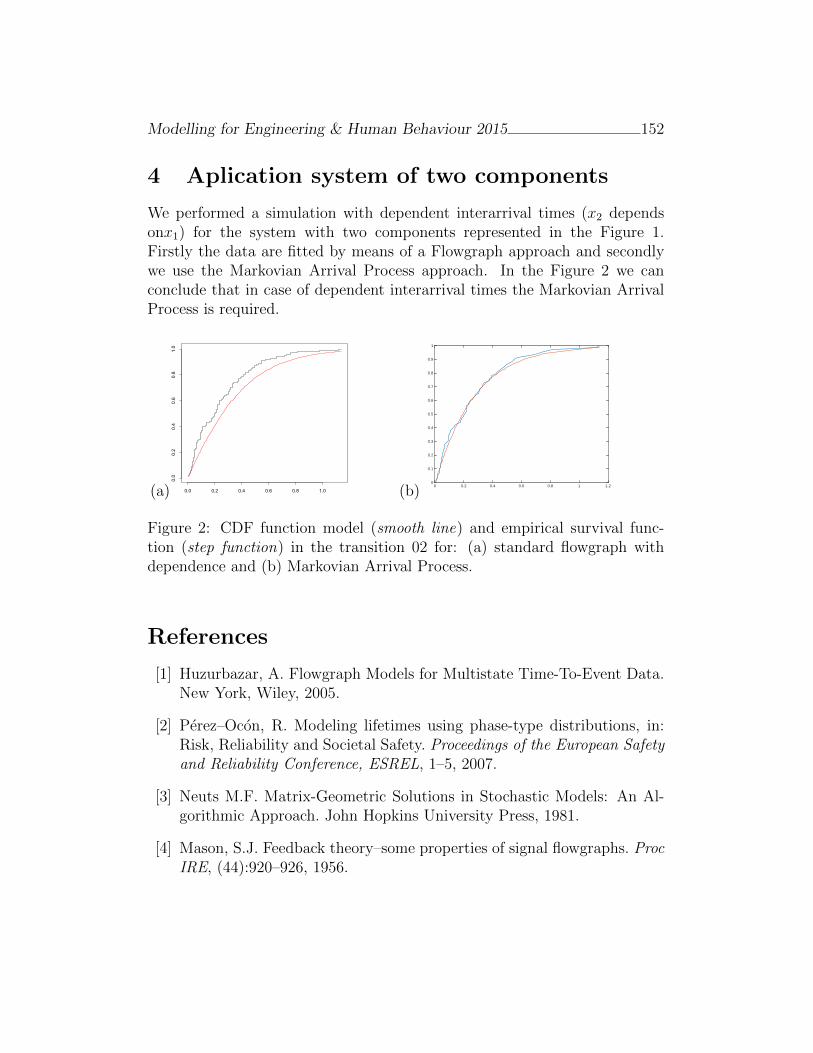
Modelling for Engineering & Human Behaviour 2015 152
4 Aplication system of two components
We performed a simulation with dependent interarrival times (x2 dependsonx1) for the system with two components represented in the Figure 1.Firstly the data are fitted by means of a Flowgraph approach and secondlywe use the Markovian Arrival Process approach. In the Figure 2 we canconclude that in case of dependent interarrival times the Markovian ArrivalProcess is required.
(a) 0.0 0.2 0.4 0.6 0.8 1.0
0.0
0.2
0.4
0.6
0.8
1.0
Time
CDF02
(b)0 0.2 0.4 0.6 0.8 1 1.2
0
0.1
0.2
0.3
0.4
0.5
0.6
0.7
0.8
0.9
1
Figure 2: CDF function model (smooth line) and empirical survival func-tion (step function) in the transition 02 for: (a) standard flowgraph withdependence and (b) Markovian Arrival Process.
References
[1] Huzurbazar, A. Flowgraph Models for Multistate Time-To-Event Data.New York, Wiley, 2005.
[2] Perez–Ocon, R. Modeling lifetimes using phase-type distributions, in:Risk, Reliability and Societal Safety. Proceedings of the European Safetyand Reliability Conference, ESREL, 1–5, 2007.
[3] Neuts M.F. Matrix-Geometric Solutions in Stochastic Models: An Al-gorithmic Approach. John Hopkins University Press, 1981.
[4] Mason, S.J. Feedback theory–some properties of signal flowgraphs. ProcIRE, (44):920–926, 1956.

Modelling for Engineering & Human Behaviour 2015 153
[5] Collins, D.H. and Huzurbazar, A.V. Prognostic models based on sta-tistical Flowgraphs. Appl. Stochastic Models Bus. Ind., (28):141–151,2012.
[6] Huzurbazar, A. and Williams, B. Incorporating Covariates in Flow-graph Models: Applications to Recurrent Event Data. Technometrics,52(2):198-208, 2010.
Hybrid wavelet support vector machine andartificial bee colony for predicting thecyanotoxin content from experimental
cyanobacteria concentrations in the Trasonareservoir: A case study in Northern Spain
P.J. Garcıa Nieto ∗, E. Garcıa-Gonzalo,J.R. Alonso Fernandez†, C. Dıaz Muniz†
() Department of Mathematics, University of Oviedo,
Faculty of Sciences, C/ Calvo Sotelo s/n, 33007 Oviedo, Spain.
(†) Cantabrian Basin Authority, Spanish Ministry of Agriculture, Food and Environment,
Plaza de Espana 2, 33007 Oviedo, Spain.
November 30, 2015
Abstract
This study presents a novel hybrid algorithm, support vector ma-chines with Mexican hat wavelet kernel function (wavelet SVMs) incombination with the artificial bee colony (ABC) technique, for pre-dicting the cyanotoxin content from cyanobacterial concentrations de-termined experimentally in the Trasona reservoir. This optimizationtechnique involves kernel parameter setting in the SVM training pro-cedure, which significantly influences the regression accuracy. Theagreement of the wavelet ABC–SVM–based model with experimen-tal data confirmed its good performance. Indeed, a coefficient of de-termination equal to 0.91 was obtained. Finally, conclusions of thisinnovative research work are exposed.
∗e-mail: [email protected]
154
Modelling for Engineering & Human Behaviour 2015 155
Keywords Support vector machines (SVMs); Wavelet kernel; Artificialbee colony (ABC); Cyanotoxins; Regression analysis
1 Introduction
Cyanobacteria, also known as blue-green algae, is a phylum of bacteriathat obtain their energy through photosynthesis. Indeed, cyanobacteria areaquatic and photosynthetic, that is, they live in the water, and can man-ufacture their own food. Sometimes, they become hazardous due to theiruncontrolled growth giving place to the formation of extensive harmful algalblooms (HABs) [1]. In addition, some cyanobacteria produce toxins calledcyanotoxins [1]. In this way, the association of toxicity with such blooms hasfrequently led to the closure of recreational waters when blooms are observed.
To fix ideas, the objective of this study is to evaluate the applicationof wavelet kernel support vector machines (SVMs) [2] in combination withthe Artificial Bee Colony (ABC) technique [3] to identify cyanotoxins in theTrasona reservoir (Principality of Asturias, Northern Spain). In recent years,the combination of wavelet theories and SVMs has drawn considerable at-tention owing to its high predictive ability for a wide range of applicationsand better performance than other traditional learning machines. In orderto carry out the optimization mechanism corresponding to the kernel op-timal hyperparameters setting in the SVM training, the artificial bee colony(ABC) technique was used here with success. The artificial bee colony (ABC)technique [3] is an optimization algorithm based on the intelligent foragingbehaviour of honey bee swarm.
2 Materials and methods
2.1 Experimental dataset
The dataset used for the SVM analysis were collected over 5 years (2006–2010)from several samples in Trasona reservoir. The total number of data pro-cessed was about 151 values (see Appendix A). Furthermore, we have takeninto account the two dominant species of the cyanobacteria community inthis research work: M. aeruginosa and W. naegeliana. It should be notedthat the main goal of this study is to obtain the dependence relationshipof cyanotoxins (output variable), expressed in micrograms per liter, as a
Modelling for Engineering & Human Behaviour 2015 156
function of the following eight biological and fifteen physical–chemical inputvariables (see Appendix A).
2.2 Support vector machine (SVM) method
In machine learning, support vector machines (SVMs) are a set of relatedsupervised learning methods used for classification and regression [4]. TheSVMs were originally developed for classification, and were later generalizedto solve regression problems. This last method is called support vector re-gression (SVR). The model produced by SVR depends on a subset of thetraining data, because the cost function for building the model ignores anytraining data that are close (within a threshold ε) to the model prediction.When the regression SVM is applied to non–linear separable data, it is ne-cessary to use the kernel trick . The reason that this kernel trick is useful isthat there are many regression problems that are not linearly regressable inthe space of the inputs x, which might be in a higher dimensionality featurespace given a suitable mapping x → ψ (x) [4].
2.3 Wavelet kernel and wavelet SVMs
Wavelet kernel SVMs refer to the wavelet kernel that combines the wavelettechnique with SVMs [2]. In this sense, the translation invariant waveletkernel so–called Mexican hat wavelet kernel is [2]:
ψ (x) =2
4√9π
·(1− x2
)· exp
(−x2
2
)
Given the above mother wavelet, the corresponding wavelet kernel functionis [2]:
K (x,x′) =N∏j=1
24√9π
(1− (xj − x′
j)2
a2
)· exp
(−(xj − x′
j)2
2a2
)
The decision function of wavelet SVMs for regression can be expressed as [2]:
f (x) =l∑
i=1
(αi − α∗i )
N∏j=1
ψ(xj − xij
a
)+ b
Specifically, the Mexican hat wavelet kernel has been used in this researchwork due to its similar shape to the HABs.
Modelling for Engineering & Human Behaviour 2015 157
2.4 The artificial bee colony (ABC) algorithm
The algorithm Artificial Bee Colony (ABC) is an evolutionary optimizationalgorithm inspired in the behaviour of the bees foraging food sources [3].Indeed, in the ABC technique, the colony consists of three groups of bees:employed bees, onlookers and scouts. It is assumed that there is only oneartificial employed bee for each food source. In other words, the number ofemployed bees in the colony is equal to the number of food sources aroundthe hive. Employed bees go to their food source and come back to hive anddance on this area. The employed bee whose food source has been abandonedbecomes a scout and starts to search for finding a new food source. Onlookerswatch the dances of employed bees and choose food sources depending ondances.
2.5 The goodness–of–fit of this approach
It is important to select the model that best fits the experimental data. Thecriterion based on the coefficient of determination (R2) was considered here[5]. A coefficient of determination value of 1.0 indicates that the regressioncurve fits the data perfectly.
3 Analysis of results and discussion
The biological and physical-chemical input variables considered in this workare shown in Appendix A. The total number of predicting variables used tobuild the hybrid wavelet kernel ABC–SVM–based model was 24. As it canbe observed one of the variables is formed by the product of the variable M.aeruginosa multiplied by the variable W. naegeliana due to the coexistenceof these two species of cyanobacteria in order to reproduce their dynamicswithout interference from external factor. This mathematical formulationadds a multiplicative additional term to account for the two species’ inter-actions according to a more realistic mathematical modelling in Biology [1].This kind of interaction (synergistic interaction) will be explained later ina more detail. All the input biological variables are measured in biovolume(cubic millimeters per liter) and the output variable (cyanotoxins) in micro-grams per liter.
Additionally, it is well known that the SVM techniques are strongly de-pendent on the SVM hyperparameters: the regularization factor C; the hy-
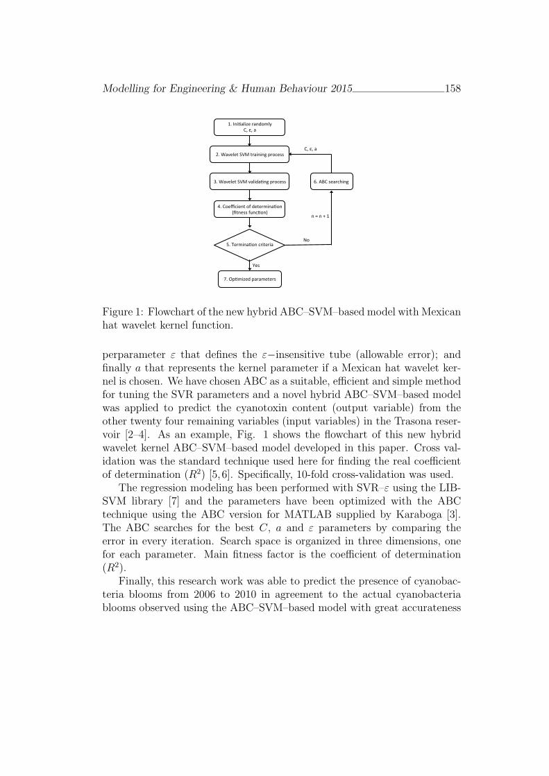
Modelling for Engineering & Human Behaviour 2015 158
!"#$%&'()&*+#,(%-./)0#
12#32#(#
4"#5(6+)+7#89:#7,(&%&%;#<,.=+>>#
?"#5(6+)+7#89:#6()&-('%;#<,.=+>>#
@"#1.+A=&+%7#.B#-+7+,/&%('.%#
CD7%+>>#BE%='.%F#
G"#HI1#>+(,=J&%;#
K"#L<'/&*+-#<(,(/+7+,>#
M"#N+,/&%('.%#=,&7+,&(#
12#32#(#
O.#
P+>#
%#Q#%#R#!#
Figure 1: Flowchart of the new hybrid ABC–SVM–based model with Mexicanhat wavelet kernel function.
perparameter ε that defines the ε−insensitive tube (allowable error); andfinally a that represents the kernel parameter if a Mexican hat wavelet ker-nel is chosen. We have chosen ABC as a suitable, efficient and simple methodfor tuning the SVR parameters and a novel hybrid ABC–SVM–based modelwas applied to predict the cyanotoxin content (output variable) from theother twenty four remaining variables (input variables) in the Trasona reser-voir [2–4]. As an example, Fig. 1 shows the flowchart of this new hybridwavelet kernel ABC–SVM–based model developed in this paper. Cross val-idation was the standard technique used here for finding the real coefficientof determination (R2) [5, 6]. Specifically, 10-fold cross-validation was used.
The regression modeling has been performed with SVR–ε using the LIB-SVM library [7] and the parameters have been optimized with the ABCtechnique using the ABC version for MATLAB supplied by Karaboga [3].The ABC searches for the best C, a and ε parameters by comparing theerror in every iteration. Search space is organized in three dimensions, onefor each parameter. Main fitness factor is the coefficient of determination(R2).
Finally, this research work was able to predict the presence of cyanobac-teria blooms from 2006 to 2010 in agreement to the actual cyanobacteriablooms observed using the ABC–SVM–based model with great accurateness
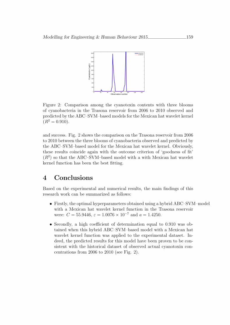
Modelling for Engineering & Human Behaviour 2015 159
0 20 40 60 80 100 120 1400
200
400
600
800
1000
1200
1400
1600
1800
Observation number
Cya
noto
xins
( µ
g/L)
observedpredicted
Figure 2: Comparison among the cyanotoxin contents with three bloomsof cyanobacteria in the Trasona reservoir from 2006 to 2010 observed andpredicted by the ABC–SVM–based models for the Mexican hat wavelet kernel(R2 = 0.910).
and success. Fig. 2 shows the comparison on the Trasona reservoir from 2006to 2010 between the three blooms of cyanobacteria observed and predicted bythe ABC–SVM–based model for the Mexican hat wavelet kernel. Obviously,these results coincide again with the outcome criterion of ‘goodness of fit’(R2) so that the ABC–SVM–based model with a with Mexican hat waveletkernel function has been the best fitting.
4 Conclusions
Based on the experimental and numerical results, the main findings of thisresearch work can be summarized as follows:
• Firstly, the optimal hyperparameters obtained using a hybrid ABC–SVM–modelwith a Mexican hat wavelet kernel function in the Trasona reservoirwere: C = 55.9446, ε = 1.0076× 10⁻⁷ and a = 1.4250.
• Secondly, a high coefficient of determination equal to 0.910 was ob-tained when this hybrid ABC–SVM–based model with a Mexican hatwavelet kernel function was applied to the experimental dataset. In-deed, the predicted results for this model have been proven to be con-sistent with the historical dataset of observed actual cyanotoxin con-centrations from 2006 to 2010 (see Fig. 2).
Modelling for Engineering & Human Behaviour 2015 160
• Finally, the synergistic variable Microcystis aeruginosa×Woronichinianaegeliana and pH values could be considered the most influential para-meters in the prediction of cyanotoxin contents in the Trasona reservoir,respectively.
Appendix A. Supplementary data
Supplementary data associated with this article can be found athttps://www.dropbox.com/s/byvcyy2smpwwv12/Trasona reservoir data sc.xls?dl=0.
References
[1] J. Huisman, H.C.P. Matthijs, P.M. Visser, Harmful Cyanobacteria, NewYork, Springer, 2010.
[2] A. Widodo, B.-S. Yang, Wavelet support vector machine for inductionmachine fault diagnosis based on transient current signal, Expert Syst.Appl. 35 (1–2):307–316, 2008.
[3] D. Karaboga, B. Basturk, A powerful and efficient algorithm for nu-merical function optimization: artificial bee colony (ABC) algorithm, J.Global Optim. 39(3):459–171, 2007.
[4] I. Steinwart, A. Christmann, Support Vector Machines, New York,Springer, 2008.
[5] D. Freedman, R. Pisani, R. Purves, Statistics, New York, W.W. Norton& Company, 2007.
[6] R. Picard, D. Cook, Cross-validation of regression models, J. Am. Stat.Assoc. 79(387):575–583, 1984.
[7] C.-C. Chang, C.-J. Lin, LIBSVM: a library for support vector machines,ACM T. Int. Syst. Technol. 2:1–27, 2011.
Valuation of commodity derivatives underjump-diffusion processes∗
L. Gomez-Valle†, Z. Habibilashkary‡, and J. Martınez-Rodrıguez§
Facultad de Ciencias Economicas y Empresariales, Universidad de Valladolid,
Avenida del Valle Esgueva, 6, 47010-Valladolid, Spain
November 30, 2015
1 Introduction
The estimation of the market prices of risk is an open question in the jump-diffusion derivative literature when a closed-form solution for the future pric-ing problem is not known. In this paper, we obtain some results that relatethe drifts and jump intensities of the risk-neutral processes with future andspot prices. These results provide an original procedure to estimate the risk-neutral drifts and jump intensities. These functions are not observable buttheir estimation is necessary for pricing commodity derivatives. Moreover,this new approach avoids the estimation of the physical drift as well as themarket prices of risk in order to price commodity futures. Finally, an appli-cation to NYMEX (New York Mercantile Exchange) data is illustrated.
∗L. Gomez-Valle and J. Martınez-Rodrıguez were supported in part by the GIR Op-timizacion Dinamica, Finanzas Matematicas y Utilidad Recursiva of the University ofValladolid and the projects and MTM2014-56022-C2-2-P of the Spanish Ministerio deEconomıa y Competitividad and European FEDER Funds and VA191U13 of the Conse-jerıa de Educacion, JCyL.†e-mail: [email protected]‡e-mail: [email protected]§e-mail: [email protected]
161
Modelling for Engineering & Human Behaviour 2015 162
2 The valuation model
In this section, we present a two-factor jump-diffusion model of commodityfuture prices. The first factor is the spot price S, and the second factoris the instantaneous convenience yield δ. Let (Ω,F ,P) be a probabilityspace equipped with a filtration F satisfying the usual conditions, [6]. Forsimplicity and tractability and as usual in the literature, we assume thatthe distribution of the jump size under Q measure, risk-neutral probabilitymeasure, is known and equal to the distribution under P measure. That is,we assume that all risk premium related to jump is artificially absorbed bythe change in the intensity of jump under the physical measure to λQS underrisk-neutral measure, see [4]. The factors of the model are assumed to followthese joint jump-diffusion stochastic processes:
dS =(µS − σSθWS
)dt+ σSdW
QS + Y dNQS , (1)
dδ =(µδ − σδθWδ
)dt+ σδdW
Qδ , (2)
where µS and µδ are the drifts under P measure, σS and σδ the volatilities,Y is the jump amplitude and it is a random variable which follows a normaldistribution N(0, σY ). Moreover, WQ
S and WQδ are the Wiener processes.
The market prices of risk of Wiener processes are θWS(S, δ) and θWδ(S, δ)and NQS represents the compensated Poisson process, under Q measure, therisk-neutral measure, with intensity λQS (S, δ) = λS(S, δ)θNS(S, δ). We assumethat the increments to standard Brownian motions are correlated with:
dWQS dW
Qδ = ρdt,
and dWQS is assumed to be independent of ˜dN
QS , which means that the diffu-
sion and jump components are independent of each other. We suppose thatall functions satisfy enough technical regularity conditions: see [5]. Underthe above assumptions, a commodity future price at time t with maturity attime T , t ≤ T , can be expressed as F (t, S, δ;T ) and at maturity is
F (T, S, δ;T ) = S. (3)
We also assume that the price of a future can be expressed by
F (t, S, δ;T ) = EQ[S(T )|Ft], (4)
Modelling for Engineering & Human Behaviour 2015 163
where EQ denotes the conditional expectation under the Q measure. Thefuture price (4) is the solution of the following partial integro-differentialequation
Ft +(µS − σSθWS
)FS +
(µδ − σδθWδ
)Fδ +
1
2σ2SFSS +
1
2σ2δFδδ + ρσSσδFSδ
+ λQSEQYS
[F (t, S + JS, δ)− F (t, S, δ)] = 0 (5)
with terminal condition (3), see the version of Feynman-Kac Dynkin lemmafor jump-diffusion processes in [3].
3 Exact results and approximations
In this section, we propose a new approach for estimating the functions of therisk-neutral jump-diffusion stochastic factors directly from data in the mar-kets. Then, as we know all the coefficients of the partial integro-differentialequation (5), we can price the future prices. Therefore, it is not necessary toestimate the market prices of risk for pricing commodity futures.
Theorem 1 Let F (t, S, δ;T ) be a solution to (5) subject to (3), and S followsa jump-diffusion process given by (1) and δ follows a diffusion process givenby (2), then:
∂F
∂T|T=t =
(µS − σSθWS
)(t), (6)
∂(SF )
∂T|T=t =
(2S∂F
∂T|T=t + σ2
S + λQSEQYS
[J2S]
)(t), (7)
∂(δF )
∂T|T=t =
(δ∂F
∂T|T=t + S(µδ − σδθWδ + ρσSσδ
)(t). (8)
Parallel results for jump-diffusion interest rate models can be found in [2].
4 Empirical application
In order to show how the approach in Section 3 can be implemented, wewill price natural gas futures with data from the NYMEX. Natural gas spotand future prices were obtained from the Energy Information Administration
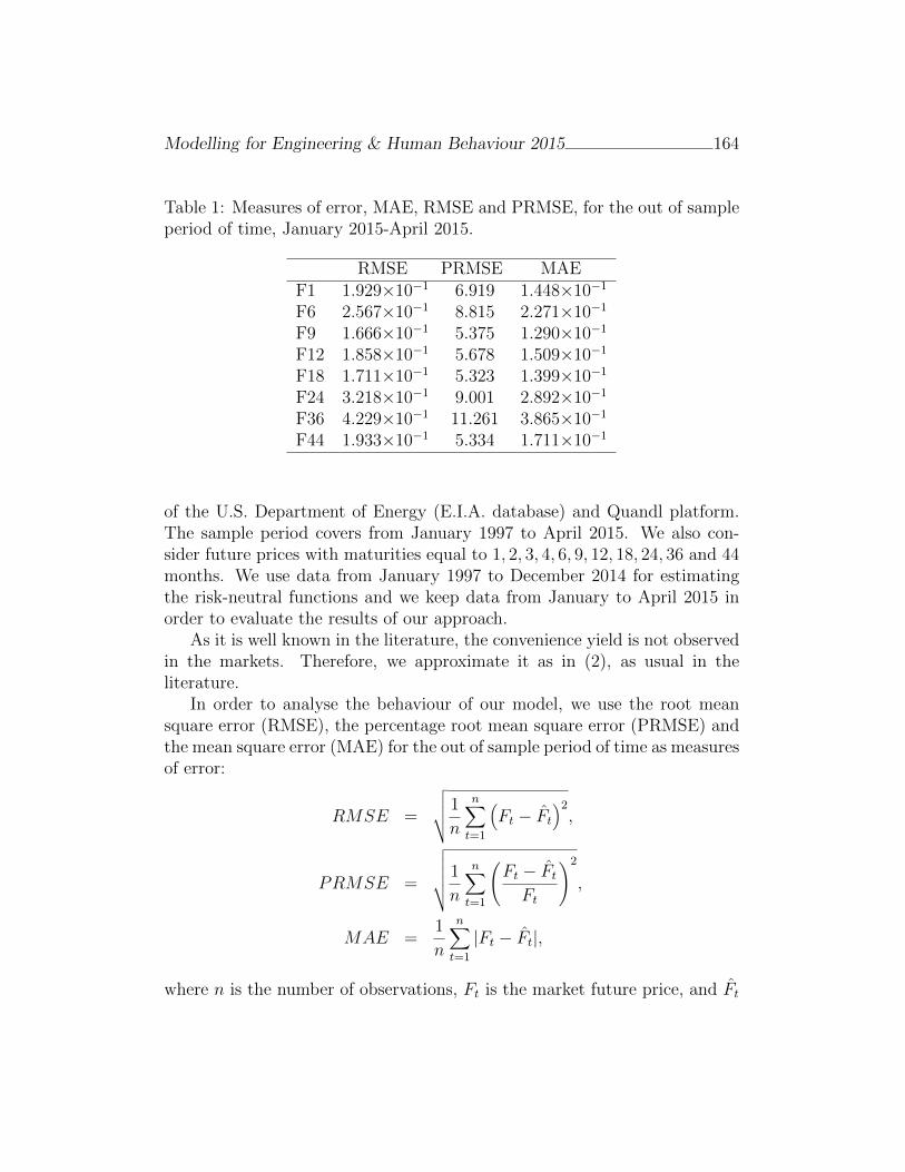
Modelling for Engineering & Human Behaviour 2015 164
Table 1: Measures of error, MAE, RMSE and PRMSE, for the out of sampleperiod of time, January 2015-April 2015.
RMSE PRMSE MAEF1 1.929×10⁻¹ 6.919 1.448×10⁻¹
F6 2.567×10⁻¹ 8.815 2.271×10⁻¹
F9 1.666×10⁻¹ 5.375 1.290×10⁻¹
F12 1.858×10⁻¹ 5.678 1.509×10⁻¹
F18 1.711×10⁻¹ 5.323 1.399×10⁻¹
F24 3.218×10⁻¹ 9.001 2.892×10⁻¹
F36 4.229×10⁻¹ 11.261 3.865×10⁻¹
F44 1.933×10⁻¹ 5.334 1.711×10⁻¹
of the U.S. Department of Energy (E.I.A. database) and Quandl platform.The sample period covers from January 1997 to April 2015. We also con-sider future prices with maturities equal to 1, 2, 3, 4, 6, 9, 12, 18, 24, 36 and 44months. We use data from January 1997 to December 2014 for estimatingthe risk-neutral functions and we keep data from January to April 2015 inorder to evaluate the results of our approach.
As it is well known in the literature, the convenience yield is not observedin the markets. Therefore, we approximate it as in (2), as usual in theliterature.
In order to analyse the behaviour of our model, we use the root meansquare error (RMSE), the percentage root mean square error (PRMSE) andthe mean square error (MAE) for the out of sample period of time as measuresof error:
RMSE =
√√√√ 1
n
n∑t=1
(Ft − Ft
)2,
PRMSE =
√√√√√ 1
n
n∑t=1
(Ft − FtFt
)2
,
MAE =1
n
n∑t=1
|Ft − Ft|,
where n is the number of observations, Ft is the market future price, and Ft
Modelling for Engineering & Human Behaviour 2015 165
is the predicted future price by our jump-diffusion model.Table 1 shows these three measures of error for the future prices along
the out of sample period of time for different maturities. Overall, the threemeasures get the highest level for futures with maturities of 24 and 36 months,i.e., for long maturities.
References
[1] Gibson, R. and Schwartz, E.S. Stochastic convenience yield and thepricing of oil contingent claims, The Journal of Finance, Volume 45 (3):959–976, 1990.
[2] Gomez-Valle, L. and Martınez-Rodrıguez, J. Estimation of risk-neutralprocesses in single-factor jump- diffusion interest rate models, Journalof Computational and Applied Mathematics, Volume 291: 48–57, 2016.
[3] Hanson F.B., Applied Stochastic Processes and Control for Jump-Diffusions. Philadelphia, SIAM, 2007.
[4] Nawalkha, S.K., Beliaeva, N., and Soto, G. , Dynamic Term StructureModelling: The Fixed Income Valuation Course. New Jersey, John Wiley& Sons, Inc, 2007.
[5] Øksendal, B., and Sulem, A., Applied Stochastic Control of Jump Dif-fusions, Berlin, Heidelberg, Springer-Verlag, 2007.
[6] Runggaldier, W.J., Jump-diffusion models, in: S.T. Rachev (Ed.),Handbook of Hevauy Tayled Distributions in Finance. Universitat Karis-ruhe, Karisruhe, North Holland, Germany, 169–209, 2003.
Applying a graph model for the SpanishPublic University System
Antonio Hervas [ ∗, Andreu Jimenez†, Pedro-Pablo Soriano †,Roberto Capilla †, Jesus Peinado†, Joan Guardia ‡, and Maribel Pero ‡
([) Universitat Politecnica de Valencia,
Instituto Universitario de Matematica Multidisciplinar ,
(†) Universitat Politecnica de Valencia ,
(‡) Universitat de Barcelona,
Institut de Recerca en Cervell, Cognicio i Conducta (IR3C).
November 30, 2015
1 Introduction
In the process of accessing the Spanish Public University System (S.U.P.E.),students applying for admission to several degrees in an orderly manner, the”system” assigns each applicant a degree and an university based on thecriteria established by the laws or is on a waiting list. Thus traffic occursbetween students who have requested a degree and is allocated to another lessdesired. This paper presents a process that allows us to model the S.U.P.E.access system using a graph, allowing us to identify some properties of thedegrees and consequently to analyze the abstract system performance.
2 Building the graph
In the S.U.P.E., after finishing the High School students must pass an exam,and then, according a polynomial formula they must apply for a degree.
∗e-mail: [email protected]
166

Modelling for Engineering & Human Behaviour 2015 167
They must select in an ordered way their options. The regional governmentassigns the positions according to their own criteria. The number of studentsdepends on regions, in Catalonia over 50.000 per year, in Valencia 25.000.
So, student applies for Degree A in first position, degree B in secondplace, another degree C in third place, and successively. We construct agraph whose vertices are the titles that are given in every university of theregion. Edge (A, B) shows that students who have applied for the grade Aas their first option have been enrolled in degree B. We assign weights basedon the percentage of students accessing to their second, third, fourth andfifth option. In Figure 1 we can see the built graph. The size of the verticesindicates the number of vacancies offered to students, the edges indicate thedirection of flow of students, and the weight of the edges indicates the valueof the flow according to the criteria discussed above.
3 Graph structure
Once obtained the graph, the first thing we did was to study the connectedcomponents.In some cases it seemed to make sense. In other cases, not atall, i.e. in engineering appear certain geographic aspects.So, we study thegraph over the point of view of communities. This concept is related withthe high density of connections in the graph, [1], [3], [2].
In a graph, a community compose a set of vertices that are highly interre-lated, meaning that there are many edges between them. In contrast, thereare few edges that connect vertices community with the rest of the graph.Or put another way, there is a high density of connections within each com-munity and a low density of connections between communities. The reasonfor using this technique is given by the fact that: ”Community structuremethods normally assume that the network of interest divides naturally intosubgroups and the experimenter’s job is to find those groups. The numberand size of the groups are thus determined by the network itself and not bythe experimenter.”, [2].
Given a network, and proposed a division of the network into commu-nities, modularity is a property that indicates how good is this division.Modularity, is a function which evaluates the goodness of partitions of agraph into clusters.[1], [4].
It is considered a good division one that gets communities have a largenumber of edges within the small communities face a number of inter-communal

Modelling for Engineering & Human Behaviour 2015 168
Figure 1: The graph for a system with 250 degrees and 25.000 students.
Figure 2: Connected component of the graph corresponding to the area ofEngineering.

Modelling for Engineering & Human Behaviour 2015 169
edges (vertices incidents these edges belong to different communities).Thereare several algorithms that allow us to get the communities on a graph, andshow us modularity, but they offer different results depending on the cri-teria for group vertices used. Also most of them apply only to undirectedgraphs.[1], [3], [5], [6] and [7].
We apply all the algorithms to our graph. Even the community lookssimilar, really the results are very different. See Figure 3.
Figure 3: Community graph under different algorithms.
4 Proposed Algorithm.
So, we propose an algorithm that finds communities in which all vertices canreach the same vertex. The main idea of operating algorithm is as follows:
• Order the vertices for the number of other vertices can be reached fromeach one, m
• In the event that m was reached by two vertices, then orders the verticesfor the number of vertices that can achieve
• Walk the ordered sequence of vertices for each vertex v marked asmembers of the same community to those from which one can reachthe vertex v, and that does not yet belong to any community.
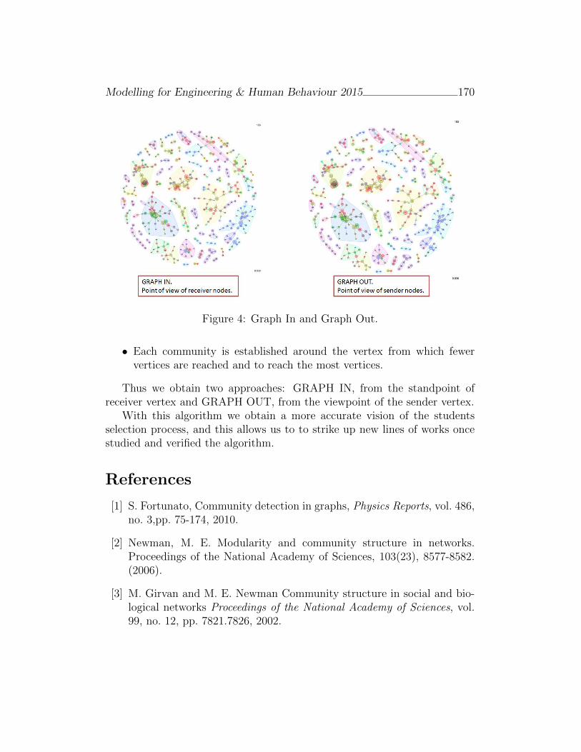
Modelling for Engineering & Human Behaviour 2015 170
Figure 4: Graph In and Graph Out.
• Each community is established around the vertex from which fewervertices are reached and to reach the most vertices.
Thus we obtain two approaches: GRAPH IN, from the standpoint ofreceiver vertex and GRAPH OUT, from the viewpoint of the sender vertex.
With this algorithm we obtain a more accurate vision of the studentsselection process, and this allows us to to strike up new lines of works oncestudied and verified the algorithm.
References
[1] S. Fortunato, Community detection in graphs, Physics Reports, vol. 486,no. 3,pp. 75-174, 2010.
[2] Newman, M. E. Modularity and community structure in networks.Proceedings of the National Academy of Sciences, 103(23), 8577-8582.(2006).
[3] M. Girvan and M. E. Newman Community structure in social and bio-logical networks Proceedings of the National Academy of Sciences, vol.99, no. 12, pp. 7821.7826, 2002.

Modelling for Engineering & Human Behaviour 2015 171
[4] M. E. Newman and M. Girvan. Finding and evaluating community struc-ture in networks Physical review E, vol. 69, no. 2, p. 026113, 2004.
[5] A. Clauset, M. E. Newman, and C. Moore Finding community structurein very large networks Physical review E, vol. 70, no. 6, p. 066111, 2004.
[6] U. N. Raghavan, R. Albert, and S. Kumara. Near linear time algorithmto detect community structures in large-scale networks. Physical ReviewE, vol. 76, no. 3,p. 036106, 2007.
[7] M. E. Newman. Finding community structure in networks using theeigenvectors of matrices Physical review E, vol. 74, no. 3, p. 036104,2006.
New iterative splitting methods for partialdifferential equations∗
J. Geiser[, J.L. Hueso†, and E. Martınez‡
([) Dept. of Electrical Engineering and Information Technology,
Ruhr-University of Bochum, Germany,
(†) Instituto de Matematica Multidisciplinar,
Universitat Politecnica de Valencia, Spain,
(‡) Instituto de Matematica Pura y Aplicada,
Universitat Politecnica de Valencia, Spain.
November 30, 2015
1 Introduction
We propose some modifications in schemes of iterative splitting techniquesfor partial differential equations and introduce the parallel version of somealgorithms. Theoretical results related to the order of the iterative splittingfor these schemes are obtained. In the numerical experiments we compare theobtained results by applying iterative methods to approximate the solutionsof the nonlinear systems obtained from the discretization of the splittingtechniques.
Iterative splitting schemes are used to solve nonlinear systems obtainedfrom ordinary differential equations or spatial discretized partial differentialequations. In their original scheme, one applies a Picard-iterative technique
∗This work has been supported by Ministerio de Ciencia e Innovacion de EspanaMTM2014-52016-C2-02.†e-mail: [email protected]
172
Modelling for Engineering & Human Behaviour 2015 173
to solve the nonlinear systems, see [2] and [3]. The drawback of such Picard’stechniques is that they are a first order scheme, see [4].
In this work, we are motivated to develop new nonlinear solvers, which aare modification of the iterative splitting schemes in [1] and [2]. Our improve-ment is finding higher order nonlinear schemes by using Newton’s method,which is embedded in the splitting methods. Such novel schemes are moreaccurate, of higher order and they accelerate the traditional solver schemes.Further, we derive parallel versions of each scheme to obtain an up to datenonlinear solver for large scale computations, see [5].
2 Splitting techniques
A great variety of natural phenomenons can be described by an ordinarydifferential equation or a partial differential equation, the solution of whichnot always can be obtained by analytical methods. In fact, in the major-ity of cases, it is much more practical using numerical methods in order toapproximate the solution.
Specifically, we deal with a particular form for PDE that can be expressedin the following form:
∂u(v, t)
∂t= A(u(v, t))u(v, t) +B(u(v, t))u(v, t) + g(v, t), (1)
where t ∈ [0, T ], the initial condition u(v, 0) = u0(v), and A(u), B(u) areoperators, in a Banach space X, involving only spatial derivatives of u, whileg(v, t) is an exterior perturbation.
In this cases, the splitting techniques can be used with the aim of substi-tute the original problem into a sequence of simpler problems, when the sizeof the problem is big, or maybe we need solve the problem taking into ac-count physical properties of some part of the equation, always with the finalobjective of building efficient methods with the usual properties of accuracyand stability.
The traditional method is the sequential operator splitting but nowadaysiterative splitting is being the objective of different studies, [6],[7]. In allcases we discretize the time interval [0, T ] in N subintervals [tn, tn+1], n =1, 2, . . . , N and solve different problems consecutively in each of these subin-tervals. Now, our aim is to introduce some modifications in the recent iter-ative splitting schemes defined in [1], and to present the parallel version ofthese algorithms.
Modelling for Engineering & Human Behaviour 2015 174
2.1 New schemes for iterative splitting
Let us consider algorithm (5.13) of [1], that is written as follows:
dui(t)
dt= A(ui−1(t))ui(t) +B(ui−1(t))ui−1(t), with ui(t
n) = u(tn),
dui(t)
dt= A(ui(t))ui(t) +B(ui(t))ui(t), with ui(t
n) = u(tn),
We propose a modification based on the idea of using the solution of firstequation ui(t) updating operators A(u) and B(u) in the second equationof the same iteration, that is, substituting A(ui−1) and B(ui−1) by A(ui)and B(ui). Moreover we consider all possible variations for combining thenonlinear operators, having four different schemes.
2.1.1 Linear Serial Iterative Splitting (LS)
dui(t)
dt= A(ui−1(t))ui(t) +B(ui−1(t))ui−1(t), with ui(t
n) = u(tn), (2)
dui(t)
dt= A(ui(t))ui(t) +B(ui(t))ui(t), with ui(t
n) = u(tn), (3)
with i = 1, 2, . . . ,m, and u0(t) is a fixed starting function that verifies theinitial condition u0(0) = u0. Once the m iterations have been performed, wetake the approximated solution u(tn+1) = um(tn+1).
2.1.2 Linear Parallel Iterative Splitting (LP)
dui(t)
dt= A(ui−1(t))ui(t) +B(ui−1(t))ui−1(t), with ui(t
n) = cn, (4)
d˜ui(t)
dt= A(ui−1(t))ui−1(t) +B(ui−1(t))˜ui(t), with ˜ui(t
n) = u(tn), (5)
and the next iteration is
ui(t) =ui(t) + ˜ui(t)
2
with i = 1, 2, . . . ,m, and u0(t) is a fixed starting function that verifies theinitial condition u0(0) = u0. Once the m iterations have been performed, wetake the approximated solution u(tn+1) = um(tn+1).
Modelling for Engineering & Human Behaviour 2015 175
2.1.3 Quasilinear Serial Iterative Splitting (QS)
dui(t)
dt= A(ui(t))ui(t) +B(ui−1(t))ui−1(t), with ui(t
n) = u(tn),
dui(t)
dt= A(ui(t))ui(t) +B(ui(t))ui(t), with ui(t
n) = u(tn),
with i = 1, 2, . . . ,m, and u0(t) is a fixed starting function that verifies theinitial condition u0(t) = 0. Once the m iterations have been performed, wetake the approximated solution u(tn+1) = um(tn+1).
2.1.4 Quasilinear Parallel Iterative Splitting (QP)
On the other hand, we can choose a parallel version, which is given as:
dui(t)
dt= A(ui(t))ui(t) +B(ui−1(t))ui−1(t), with ui(t
n) = u(tn),
d˜ui(t)
dt= A(ui−1(t))ui−1(t) +B(˜ui(t))˜ui(t), with ˜ui(t
n) = u(tn),
and the next iteration is
ui(t) =ui(t) + ˜ui(t)
2
with i = 1, 2, . . . ,m, and u0(t) is a fixed starting function that verifies theinitial condition u0(t) = 0.
Once the m iterations have been performed, we take the approximatedsolution u(tn+1) = um(tn+1).
3 Theoretical results
In this section we obtain the convergence order for the different algorithmsand the expressions for the local error.
Theorem 3.1. We assume to have bounded nonlinear operators A and B,while given as ||A(u)|| ≤ Amax and ||B(u)|| ≤ Bmax for all u ∈ X.
Then the numerical errors after m iterations are given for the differentschemes as:
Modelling for Engineering & Human Behaviour 2015 176
1. Serial version, the numerical error is given as:
||em(τ)|| ≤ AmmaxB
mmaxO(τ 2m),
2. Parallel version, the numerical error is given as:
||em(τ)|| ≤ (Amax
2+Bmax
2)mO(τm).
4 Numerical experience
We compare different splitting schemes applied to two examples, the mixedconvection-diffusion and Burgers’ equation and a momentum equation thatmodels a viscous flow. The differential equations in each splitting intervalare solved by using the back-Euler-Newton algorithm.
It is worth mentioning that one step of Newton’s method suffices to reachan approximate solution of the implicit Euler method in each splitting inter-val. Additional steps do not produce a significant error reduction. Thus, inthe numerical examples, only one Newton’s step is performed.
References
[1] J. Geiser. Modified Jacobian Newton Iterative Method: Theory and Ap-plications. Mathematical problems in Engineering, Hindawi PublishingCorporation, (2009), Article ID 307298.
[2] J. Geiser. Iterative Splitting Methods for Differential Equations. Chap-man & Hall/CRC Numerical Analysis and Scientific Computing Series,ed. Magoules and Lai, 2011.
[3] O. Nevanlinna. Remarks on Picard-Lindelof Iteration: Part I, BIT 29(1989) 328–346.
[4] C.T. Kelly. Iterative Methods for Linear and Nonlinear Equations. Fron-tiers in Applied Mathematics, SIAM, Philadelphia, PA, 1995.

Modelling for Engineering & Human Behaviour 2015 177
[5] M.J. Gander. 50 Years of Time Parallel Time Integration, T. Carraro,M. Geiger, S. Korkel, R. Rannacher, to appear in Multiple Shooting andTime Domain Decomposition, Springer Verlag, 2015.
[6] I. Farago and J. Geiser. Iterative Operator-Splitting methods for LinearProblems, Preprint No. 1043 of Weierstrass Institute for Applied Anal-ysis and Stochastics, Berlin, Germany, 2005.
[7] J. Geiser. Iterative Operator-Splitting Methods with higher order Time-Integration Methods and Applications for Parabolic Partial Differen-tial Equations, Journal of Computational and Applied Mathematics 217,(2008), 227–242.
Real-time water demand forecasting using
support vector machine and adaptive Fourier
series
B. Brentan⋆ ∗, E. Luvizotto Jr.⋆, M. Herrera † J. Izquierdo
and R. Perez-Garcıa
(⋆)Computaional Hydraulic Laboratory, University of Campinas, Brazil
(†) EDEn - Dept. of Architecture and Civil Eng., University of Bath, UK
() Fluing - IMM, Universitat Politecnica de Valencia, Spain
November 30, 2015
1 Introduction
Both safe operations of water supply systems (WDSs) and design of newWDSs require water demand forecasting. For a monitored WDS, the use ofdata can provide deep knowledge on water demand and become a powerfulmanagement tool to improve system efficiency.
ARIMA models have been traditionally applied for modeling water de-mand. However this approach usually considers linear correlations amongvariables. This hypothesis not always help develop a model able to makepredictions with required accuracy, thus harming control processes. Recentworks propose the use of artificial intelligence and machine learn tools tomodel the non-linearity among the variables. [?] compare various predictivemethods applied to hourly water demand forecasting, suggesting support vec-tor machine as one of the best models. The arrival of new data can becomeobsolete in off-line models and the application to operation modes requiresgreat improvement of accuracy, which can be obtained by on-line models.
178
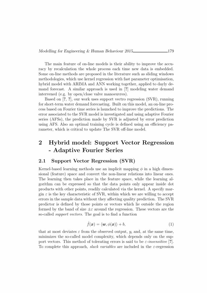
Modelling for Engineering & Human Behaviour 2015 179
The main feature of on-line models is their ability to improve the accu-racy by recalculation the whole process each time new data is embedded.Some on-line methods are proposed in the literature such as sliding windowsmethodologies, which use kernel regression with fast parameter optimisation,hybrid model with ARIMA and ANN working together, applied to dayly de-mand forecast. A similar approach is used in [?] modeling water demandintervened (e.g. by open/close valve manoeuvres).
Based on [?, ?], our work uses support vectro regression (SVR), runningfor short-term water demand forecasting. Built on this model, an on-line pro-cess based on Fourier time series is launched to improve the predictions. Theerror associated to the SVR model is investigated and using adaptive Fourierseries (AFSs), the prediction made by SVR is adjusted by error predictionusing AFS. Also an optimal training cycle is defined using an efficiency pa-rameter, which is critical to update The SVR off-line model.
2 Hybrid model: Support Vector Regression
- Adaptive Fourier Series
2.1 Support Vector Regression (SVR)
Kernel-based learning methods use an implicit mapping φ in a high dimen-sional (feature) space and convert the non-linear relations into linear ones.The learning then takes place in the feature space, while the learning al-gorithm can be expressed so that the data points only appear inside dotproducts with other points, readily calculated via the kernel. A specify mar-gin ε is the key characteristic of SVR, within which we are willing to accepterrors in the sample data without they affecting quality prediction. The SVRpredictor is defined by those points or vectors which lie outside the regionformed by the band of size ±ε around the regression. These vectors are theso-called support vectors. The goal is to find a function
f(x) = 〈w, φ(x)〉+ b, (1)
that at most deviates ε from the observed output, yi and, at the same time,minimizes the so-called model complexity, which depends only on the sup-port vectors. This method of tolerating errors is said to be ε-insensitive [?].To complete this approach, slack variables are included in the ε-regression

Modelling for Engineering & Human Behaviour 2015 180
fostering the chances to achieve better predictions in a more relaxed space.
2.2 Adaptive Fourier Series (AFS)
The Fourier series set of equations presented here is based on [?], wheretrigonometric adjustment is applied to data coming from both equally andnot-equally spaced measurements. Taking equally spaced values of t in theperiod of interest, and normalizing times to the interval [0 , 2π], the error ebetween the real deviation d and the Fourier value at time step ti is written
e =
N−1∑
i=0
f(ti)− [a0 +
M∑
j=1
aj · cos(jti) +
M∑
j=1
bj · sin(jti)]2. (2)
where M is the length of the Fourier polynomial, and a0, aj and bj are theadjustable Fourier coefficients.
Applying, the least square method to minimize e, taking into accountobvious orthogonality conditions, it is possible to obtain each adjustablecoefficient of the series.
2.3 Hybrid model
The hybrid model can be fast enough to respond to abrupt changes in wa-ter demand conditions. Using SVR for standard prediction, we propose anadditive layer, the Fourier layer, to adjust the deviation. First, a calibrationprocess is required to define the SVR parameters:
• Parameter C, which gives a trade-off between model complexity andthe amount up to which deviations larger than ε are tolerated, alsoresponsible of the robustness of the regression model.
• Parameter ε, which regulates the radius of the ε-tube around the re-gression function.
To train the model, a mesh is created with pairs of ǫ and C, with correspond-ing ranges: 0.05 ≤ ǫ ≤ 0.9 and 1 ≤ C ≤ 1500. A Grid Search Method isapplied to tune the parameters, in which each pair represent a possible ofsolution.
Once tuned, the model is running and the deviations d between predictedand observe demand are computed. Deviation is typically larger at demand
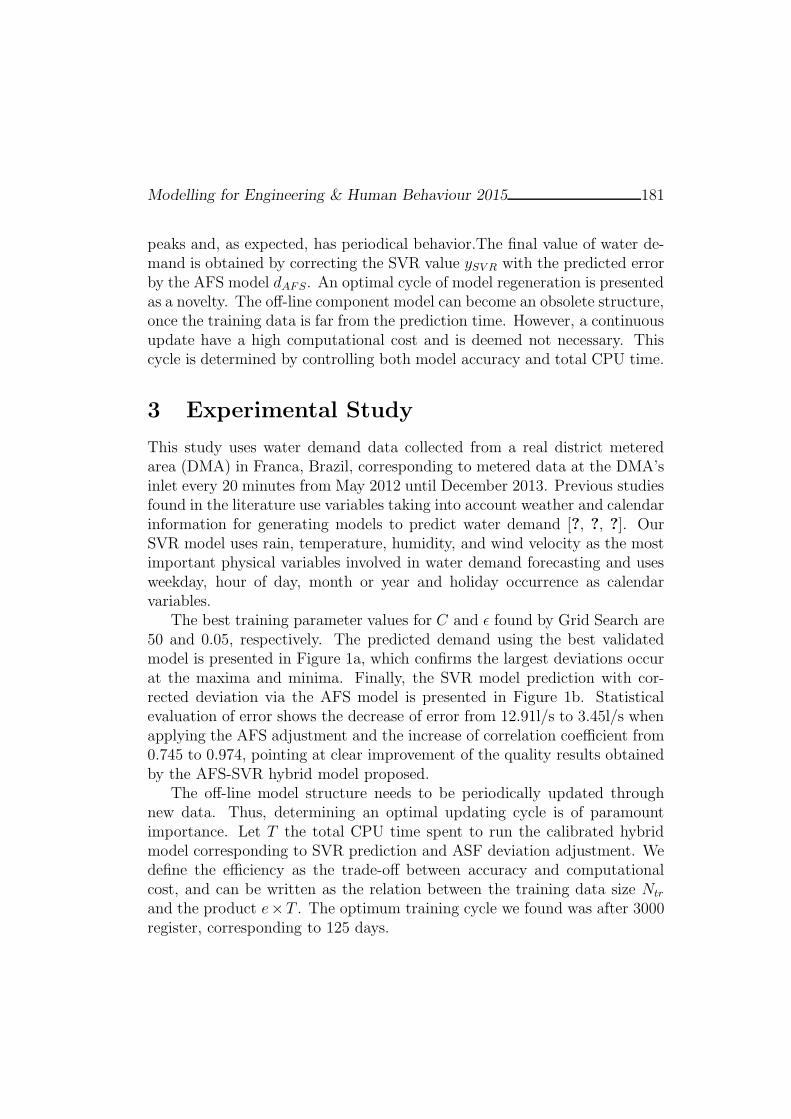
Modelling for Engineering & Human Behaviour 2015 181
peaks and, as expected, has periodical behavior.The final value of water de-mand is obtained by correcting the SVR value ySVR with the predicted errorby the AFS model dAFS. An optimal cycle of model regeneration is presentedas a novelty. The off-line component model can become an obsolete structure,once the training data is far from the prediction time. However, a continuousupdate have a high computational cost and is deemed not necessary. Thiscycle is determined by controlling both model accuracy and total CPU time.
3 Experimental Study
This study uses water demand data collected from a real district meteredarea (DMA) in Franca, Brazil, corresponding to metered data at the DMA’sinlet every 20 minutes from May 2012 until December 2013. Previous studiesfound in the literature use variables taking into account weather and calendarinformation for generating models to predict water demand [?, ?, ?]. OurSVR model uses rain, temperature, humidity, and wind velocity as the mostimportant physical variables involved in water demand forecasting and usesweekday, hour of day, month or year and holiday occurrence as calendarvariables.
The best training parameter values for C and ǫ found by Grid Search are50 and 0.05, respectively. The predicted demand using the best validatedmodel is presented in Figure 1a, which confirms the largest deviations occurat the maxima and minima. Finally, the SVR model prediction with cor-rected deviation via the AFS model is presented in Figure 1b. Statisticalevaluation of error shows the decrease of error from 12.91l/s to 3.45l/s whenapplying the AFS adjustment and the increase of correlation coefficient from0.745 to 0.974, pointing at clear improvement of the quality results obtainedby the AFS-SVR hybrid model proposed.
The off-line model structure needs to be periodically updated throughnew data. Thus, determining an optimal updating cycle is of paramountimportance. Let T the total CPU time spent to run the calibrated hybridmodel corresponding to SVR prediction and ASF deviation adjustment. Wedefine the efficiency as the trade-off between accuracy and computationalcost, and can be written as the relation between the training data size Ntr
and the product e×T . The optimum training cycle we found was after 3000register, corresponding to 125 days.
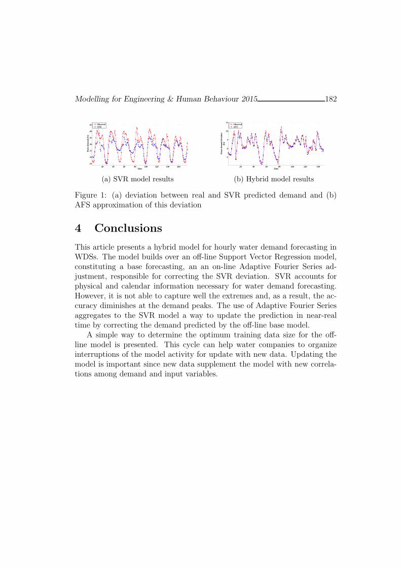
Modelling for Engineering & Human Behaviour 2015 182
20 40 60 80 100 120 140 16015
20
25
30
35
40
45
Time
Wat
er d
eman
d (l/
s)
ObservedSVR
(a) SVR model results
20 40 60 80 100 120 140
−5
0
5
10
15
Time
Wat
er d
eman
d de
viat
ion
(l/s)
ObservedAFS
(b) Hybrid model results
Figure 1: (a) deviation between real and SVR predicted demand and (b)AFS approximation of this deviation
4 Conclusions
This article presents a hybrid model for hourly water demand forecasting inWDSs. The model builds over an off-line Support Vector Regression model,constituting a base forecasting, an an on-line Adaptive Fourier Series ad-justment, responsible for correcting the SVR deviation. SVR accounts forphysical and calendar information necessary for water demand forecasting.However, it is not able to capture well the extremes and, as a result, the ac-curacy diminishes at the demand peaks. The use of Adaptive Fourier Seriesaggregates to the SVR model a way to update the prediction in near-realtime by correcting the demand predicted by the off-line base model.
A simple way to determine the optimum training data size for the off-line model is presented. This cycle can help water companies to organizeinterruptions of the model activity for update with new data. Updating themodel is important since new data supplement the model with new correla-tions among demand and input variables.
Effects of the obesity on optimal controlschedules of chemotherapy on a cancerous
tumor
S.E. Delgadillo[ ∗, R.A. Ku-Carrillo†, and B.M. Chen-Charpentier‡
([, † )Departamento de Matematicas y Fısica, Universidad Autonoma de Aguascalientes
Av. Universidad 940, Cd. Universitaria, Aguascalientes, Mexico
(‡) Department of Mathematics, University of Texas at Arlington,
Arlington, TX 76019, USA
November 30, 2015
1 Introduction
In this work, we propose and analyze a cancer-obesity model for the growthof a tumor where chemotherapy schedules are obtained using optimal controltechniques. Our aim is to study how the obesity can affect different tumorgrowth scenarios when chemotherapy is applied. This was motivated bythe reported relationship between obesity and cancer in several experimentalstudies such as [1, 2, 3, 4]. Among the cancers that present this relationshipare colorectal cancer, breast cancer in postmenopausal women, endometriumcancer, renal cancer, and esophagus cancer [5].
Our model incorporates an equation for stored fat in the organism bymeans of a logistic equation. It is well known that this equation includes acoefficient to model the carrying capacity which could be related to the fatstored in the organism. In order to get some insights about this problem,this model proposes a mathematical interaction between the stored fat in the
∗e-mail: [email protected]
183
Modelling for Engineering & Human Behaviour 2015 184
organism and the cancerous tumor. We consider that an increment of fat inthe organism increases the growth rate of the tumor. Another aspect thatour model expects to capture is the dynamics of the immune system cells,particularly the T8 cells related to the regress of small tumor. In this case,the immune response is a natural control that kills tumor cells in order tokeep a healthy organism.
A literature review of the models of obesity and cancer shows differentapproaches. Close related models to ours are those which take into accountthe immune system and the tumor cells populations such as [7, 8], Kirschnerand Panetta [9], and Bellomo [10]. Even though this list is not exhaustive,it illustrates the wide variety of immune cancer models. Our model proposalis based on De Pillis and Radunskaya model, reported in [7, 8] which alsomodels the chemotherapy treatment using control theory.
2 The cancer-obesity model with chemother-
apy
The model that we study in this work is the following:
I = s+ρIT
α + µF + T− c1IT − d1I − a1(1− e−u)I
T = r1T (1− b1T )− c2IT − c3TN + c5TF − a2(1− e−u)T
N = r2N(1− b2N)− c4TN − a3(1− e−u)N
F = r3F (1− b3F )− c6FT − a4(1− e−u)F,
u = v − d2u (1)
where I(t) denotes the number of immune cells at time t, T (t) is the numberof tumor cells at time t, N(t) the number of normal cells at time t, F (t) isthe fat stored in adipocytes at time t, and u(t) is the drug in the organism.The function v(t) models the application protocol of chemotherapy. Theparameters associated to the immune system are s, the basal response, andρ, the immune response stimulated by the cancer cells. The constants r1,r2 and r3 are the growth rates for the tumor cells, the normal cells andthe fat, respectively. The competition terms are the constants c1, c2, c3, c4between the different populations and c5 is the contribution of the fat to thecancerous cells growth. Finally, the constants a1, a2, a3, and a4 model thekill effectiveness of the drug on I, T , N and F populations, respectively.

Modelling for Engineering & Human Behaviour 2015 185
The equilibrium analysis of model (1) without the presence of chemother-apy is important to understand the dynamics of the system, i.e. whenu(t) = 0 for all t. Let us mention, that the model has been normalizedin such a way that b2.
The equilibrium points can be classified depending on whether there ispresence of fat (F = 1/b3) or not (F = 0). The following equilibrium pointsarise in the model (1) with the condition, F = 1/b3 obtained by solving theassociated nullclines system.
• Dead: PO1 = ( sd1, 0, 0, 1
b3). Only immune cells and fat are present. It
is easy to verify that this equilibrium point is always unstable.
• Total cancer invasion: PO2 = (I, T, 0, 1b3
) represents a case of deathbecause there are not normal cells. The stability of the equilibriumpoint changes depending on the parameter values.
• Tumor-free: PO3 = ( sd1, 0, 1
b2, 1b3
) represents the case of health becausethe tumor density is zero. This point is stable when r1 + c5
b3< c2s
d1+
c3b2
. The stability condition depends on the tumor growth rate, theinteraction coefficients and the basal source rate of the immune system.
• Coexistence: PO4 = (I, T,N, 1b3
). In these equilibria all types of cellscoexist and there can be zero, one, two or three points depending on theparameter values. The stability might vary depending on the parametervalues.
For the case when there is not presence of fat F = 0 we found the sametype of equilibria, but they are all unstable because the growth rate of thefat is positive, r3 > 0.
3 Optimal control application
Our optimal control problem consists in finding a function v(t) such as thecancer cell population T hits a minimum at a given time tf while the densityof normal cells is greater than 0.75 for all t. We look for minimizing theobjective function:
J(tf ) = T (tf ),
Modelling for Engineering & Human Behaviour 2015 186
restricted to keeping the normal cells population above 0.75 :
N(t) ≥ 0.75, 0 ≤ t ≤ tf .
For simplicity, we denote the state variables by (I, T,N, F, u) = (x1, x2, x3, x4, x5).If tf is the final time, the optimal control problem will be:
Min J(x, v) = x2(tf ),
subject to the equation system (1) and the following constrain:
k(x, t, v) = x3(t)− 0.75 ≥ 0, 0 ≤ t ≤ tf . (2)
The associated hamiltonian for the optimal control problem is:
H = p1(x1) + p2(x2) + p3(x3) + p4(x4) + p5(x5) + ηk,
where the functions pi = − ∂H∂xi, or explicitly:
p1 = −p1(
ρx2α + x2 + µx4
− c1x2 − d1 − a1(1− e−x5)
)+ p2c2x2
p2 = −p1(
(α + µx4)ρx1(α + x2 + µx4)2
− c1x1)− p2(r1 − 2r1b1x2 − c2x1 − c3x3 + c5x4
− a2(1− e−x5)) + p3c4x3 + p4c6x4
p3 = p2c3x2 − p3(r2 − 2r2b2x3 − c4x2 − a3(1− e−x5)
)− η(t)
p4 = p1
(ρx1x2µ
(α + x2 + µx4)2
)− p2c2x2 − p4
(r3 − 2r3b3x4 − c6x2 − a4(1− e−x5)
)p5 = e−x5 (p1a1x1 + p2a2x2 + p3a3x3 + p4a4x4) + p5d2, (3)
where η(t) ≤ 0 with η(t)k(t) = 0.
η(t) =
−1 if x3(t) ≤ 0.75
0 other case.(4)
The boundary values for the co-state variables are:
p1(tf ) = 0, p2(tf ) = 1, p3(tf ) = 0, p4(tf ) = 0, p5(tf ) = 0.
Modelling for Engineering & Human Behaviour 2015 187
Finally, the control equation is given by,
∂H
∂v= p5 = 0,
for 0 ≤ v(t) ≤ 1. Bang-bang type solutions are compatible with this system,
v(t) =
0 p5 > 01 p5 < 0.
(5)
We carried out numerical experiments to determine the optimal chemother-apy schedules using parameters reported in the literature.
4 Conclusions
A mathematical model for the effect of obesity on the tumor growth, andconsequently, on the optimal control chemotherapy schedules has been dis-cussed in this paper. The numerical experiments showed that the effectsof losing weight can be adjuvant to the chemotherapy treatment, and also,that weight gain can cause a lesser reduction of the tumor when is appliedchemotherapy. Specific examples of such effects were presented in paper.
References
[1] Rubin, H., Promotion and selection by serum growth factors drive fieldcancerization, which is anticipated in vivo by type 2 diabetes and obesity,Proceedings of the National Academy of Sciences, 110(34): 13927-13931,2013.
[2] Ehsanipour, E.A. and Sheng, X. and Behan, J.W. and Wang, X. andButturini, A. and Avramis, V.I. and Mittelman, S.D., Adipocytes causeleukemia cell resistance to L-asparaginase via release of glutamine, Can-cer research, 73(10): 2998-3006, 2013.
[3] Taubes, G., Unraveling the obesity-cancer connection, Science,335(6064): 28-32, 2012.
[4] Hursting, S.D., Minireview: The Year in Obesity and Cancer, MolecularEndocrinology 26(12): 1961-1966, 2012.

Modelling for Engineering & Human Behaviour 2015 188
[5] Schwab, M., Encyclopedia of cancer, Berlin Heidelberg, Springer, 2016.
[6] Zhang, X., Wu, W.and Yu, J., Obesity and Cancer. Zurich SpringerInternational Publishing, 2016.
[7] De Pillis, L.G. and Radunskaya, A., A mathematical tumor model withimmune resistance and drug therapy: an optimal control approach,Computational and Mathematical Methods in Medicine, 3(2): 79-100,2001.
[8] De Pillis, L.G. and Radunskaya, A., The dynamics of an optimally con-trolled tumor model: A case study, Mathematical and Computer Mod-elling, 37(11):1221-1244, 2003.
[9] Kirschner, D. and Panetta, J.C., Journal of mathematical biology 37(3):235-252, 1998.
[10] Bellomo, N. and Li, N.K. and Maini, P.K., On the foundations of cancermodelling: selected topics, speculations, and perspectives, MathematicalModels and Methods in Applied Sciences, 18(04): 593–646, 2008.
Convergence results for an optimalfourth-order family of methods presented by
Sharma
I. K. Argyros[, A. Cordero†, A. A. Magrenan‡ ∗and J. R. Torregrosa†
([) Cameron University,
73505 Lawton, OK, USA
(†) Universitat Politecnica de Valencia,
46022 Valencia, Spain
(‡) Universidad Internacional de La Rioja (UNIR),
Av. Gran Vıa Rey Juan Carlos I, 41, 26002 Logrono, La Rioja, Spain.
November 15, 2015
1 Introduction
In this study, we are concerned with the problem of approximating a solutionx∗ of the nonlinear equation
F (x) = 0 (1)
where F is a differentiable operator defined on a subset Ω of X with values inY . Using mathematical modelling, many problems in computational sciencesand other disciplines can be brought in a form like (1). The solutions of theseequations (1) can rarely be found in closed form. Therefore solutions of theseequations (1) are approximated by iterative methods.
In this work, we consider the following family of methods defined by
∗e-mail: [email protected]
189

Modelling for Engineering & Human Behaviour 2015 190
Sharma in [6] for each n = 0, 1, 2, . . . by
yn = xn −2
3
F (xn)
F ′ (xn)
zn = xn −F ′ (xn) + 3F ′ (yn)
−2F ′ (xn) + 6F ′ (yn)
F (xn)
F ′ (xn)
xn+1 = xn −F ′ (xn) + aF ′ (yn)
bF ′ (xn) + cF ′ (yn)
F (zn)
F ′ (xn)
(2)
where a, b, c are parameters.
2 Convergence result
We shall study the local convergence analysis of method defined for eachx = 0, 1, 2 . . .
yn = xn − ξF ′ (xn)−1 F (xn)
zn = xn − λA−1n F ′ (xn)−1 F (xn)
xn+1 = zn − µB−1n F ′ (xn)−1 F (zn)
(3)
where x0 is an initial point, ξ, λ, µ are parameters,
An = 2 (F ′ (xn) + 3F ′ (yn))−1
(F ′ (xn)− 3F ′ (yn))
andBn = (F ′ (xn) + aF ′ (yn))
−1(bF ′ (xn) + cF ′ (yn)) .
Theorem 2.1 Let F : D ⊂ X → Y be a Frechet-differentiable operator.Suppose that there exist x∗ ∈ D, L0 > 0, L > 0, M0 > 0, M ≥ 1, α > 0,a ∈ S \ −1,b, c, ξ, λ, µ ∈ S such that for all x, y ∈ D the followingconditions hold:
M |1− ξ| < 1,
p (0)M0
4(1 + |µ|M) < 1,
F (x∗) = 0, F ′ (x∗)−1 ∈ L (Y,X) , ‖F ′ (x∗) ‖ ≤ α, (4)
‖F ′ (x∗)−1 (F ′ (x)− F ′ (x∗)) ‖ ≤ L0‖x− x∗‖, (5)
‖F ′ (x∗)−1 (F ′ (x)− F ′ (y)) ‖ ≤ L‖x− y‖, (6)
‖F ′ (x) ‖ ≤M0, (7)

Modelling for Engineering & Human Behaviour 2015 191
‖F ′ (x∗)−1 F ′ (x) ‖ ≤M, (8)
andU (x∗, r) ⊆ D, (9)
where functions p and ϕ are defined as:
p (t) = 4M (2 +M0|λ|) , if λ 6= 0
orp (t) = 0, if λ = 0,
and
ϕ (t) =|1 + b|L0 (1 + g1 (t)) t
|1 + a|(
1−(
L0
|1 + a|(1 + |a|g1 (t)) t
)t
) , if a+ b+ c+ 1 = 0
or
ϕ (t) =(|1 + b|+ |a+ c|)M
|1 + a|(
1−(
L0
|1 + a|(1 + |a|g1 (t)) t
)t
) , if (|1 + b|+ |a+ c|)M < |1+a|
where,
g1 (t) =1
2 (1− L0t)[Lt+ 2M |1− ξ|]
Moreover, we define
γ (t) =3L0 (1 + g1 (t)) t
4
(1− L0
4(1 + 3g1 (t)) t
) ,and r is the minimum of
• 2 (1−M |1− ξ|)2L0 + L
.
• The smallest positive root of:
3L0 (1 + g1 (t)) t+ L0 (1 + 3g1 (t)) t− 4 = 0

Modelling for Engineering & Human Behaviour 2015 192
• The smallest positive root of:
1
2 (1− L0t)
Lt+M0p (t)
2
(1−
((L0
4(1 + 3g1 (t))
)t
)(1− γ (t))
)−1 = 0
• The smallest positive root of:
L0
|1 + a|(1 + |a|g1 (t)) t− 1 = 0
• The smallest positive root of:
|1 + b|L0 (1 + g1 (t)) t+ |1 + a|(
L0
|1 + a|(1 + |a|g1 (t)) t
)t− |1 + a| = 0.
• The smallest positive root of: 1
2 (1− L0t)
Lt+M0p (t)
2
(1−
(L0
4(1 + 3g1 (t))
)t
)(1− γ (t))
×[1 +
|µ|M(1− L0t) (1− ϕ (t))
]− 1 = 0.
Then, sequence xn generated for x0 ∈ U (x∗, r)\x∗ by method (3) is welldefined, remains in U (x∗, r) for each n = 0, 1, 2, . . . and converges to x∗.
As family (3) is a parametric family, we can study the dynamics by menasof using the techniques presented in [1, 2, 3, 4, 5].
References
[1] I. K. Argyros, A. A. Magrenan, On the convergence of an optimal fourth-order family of methods and its dynamics, Appl. Math. Comput. 252(1),336–346 (2015).

Modelling for Engineering & Human Behaviour 2015 193
[2] F. Chicharro, A. Cordero, J.R. Torregrosa, Drawing dynamical and pa-rameters planes of iterative families and methods, The Scientific WorldJournal Volume 2013 Article ID 780153.
[3] A. Cordero, J. Garcıa-Maimo, J.R. Torregrosa, M.P. Vassileva, P. Vin-del, Chaos in King’s iterative family, Applied Mathematics Letters 26(2013) 842–848.
[4] A. A. Magrenan, Different anomalies in a Jarratt family of iterative root-finding methods, Applied Mathematics and Computation 233 (2014),29–38.
[5] A. A. Magrenan, A new tool to study real dynamics: The convergenceplane Applied Mathematics and Computation, 248 (2014), 215–224.
[6] R. Sharma, Iterative methods for the solution of nonlinear equations(PhD Thesis), Punjab University, 2011.
A Two-level ILU preconditioner forelectromagnetism applications
J. Cerdan∗, J. Marın and J. MasInstituto de Matematica Multidisciplinar
Universitat Politecnica de Valencia, Camı de Vera s/n 46022 Valencia Spain
1 Introduction
The numerical solution of the Maxwell’s equations [7] plays a crucial rolein numerous large scale industrial and scientific applications related withelectromagnetism phenomena. To name a few, the computation of the an-tenna radiation pattern, electromagnetic interference and compatibility stud-ies of an electrical device with their environment, and scattering problemsas the computation of the radar cross-section of 3D body are important foraerospace industry.
The most common techniques for obtaining a numerical solution of Maxwell’sequations can be classified either into methods that solve the differentialequations or methods that consider their integral formulation. Integral equa-tions methods (IEMs) have emerged as an attractive alternative for CEM ap-plications. These methods solve the problem by reformulating the Maxwell’sequations as a set of integral equations with equivalent sources [2]. The inte-gral equations relate the electric and magnetic fields to the equivalent electricand magnetic currents on the surface of the object. This leads to a reductionon the dimensionality of the problem by one, and therefore allows signifi-cant reduction on the number of unknowns of the associated linear systems.Because the boundary conditions are incorporated into the surface integralequations, IEMs can handle general geometries in open domains withoutformulating any artificial boundary.
∗e-mail: [email protected]
194
Modelling for Engineering & Human Behaviour 2015 195
The integral equations are usually discretized by means of the boundaryelement method (BEM) or the Method of Moments (MoM) [8]. The matri-ces arising from IEMs are dense and expensive to solve. Since in large-scaleindustrial applications the size of the matrices can be very large the applica-tion of direct gaussian elimination methods is out of context, leaving the useof Krylov-type iterative methods as the only practical alternative. As it iswell known, the success of an iterative method for ill-conditioned problemsdepends on applying a suitable preconditioning technique to the system ma-trix. In [1] the author show that most algebraic factorized preconditionersfail to produce good converge rates or even fail to converge. The best resultson medium size problems were obtained with sparse approximate inversepreconditioners based on Frobenious norm minimization [5].
Our aim in this work is to present a technique for the compuation ofILU-type preconditioners for ill-conditioned CEM applications. The methodis based on graph partitioning techniques applied to the near field matrixof the linear systems. The paper is organized as follows. In Sections 2and 3 we review the main ideas of graph partitioning and the algorithmfor computing a two-level ILU for CEM applications. Then, the numericalresults are presented in Section 4.
2 Graph partitioning
The idea behind graph partitioning is the computation of a p−way partition-ing of the adjacency graph of a matrix keeping the size of the p subgraphsbalanced while minimizing to some extent the number of edges that are cut.Let A be a sparse structurally symmetric matrix. The associated undirectedadjacency graph G = (V,E) consists of a set nodes V = 1, . . . , n, one nodefor each row or column of the matrix, and the edge set E. There is an edge〈i, j〉 for any matrix entry aij 6= 0. Note that there is not distinction between〈i, j〉 and 〈j, i〉. For nonsymmetric sparse patterns the adjacency graph ofA + AT is considered instead. We define the separator set as the group ofnodes which are connected by edges that are cut in the graph partition. Wealso define the group of interior nodes as the nodes which are connected withthe separator set. Thus, there are p groups of interior nodes, one for eachsubgraph of the partition. By numbering first the interior nodes and tak-ing the separator set last, the matrix is permuted into the following block
Modelling for Engineering & Human Behaviour 2015 196
angular form:
P TAP =
A1 B1
A2 B2
. . ....
Ap Bp
C1 C2 . . . Cp AS
(1)
where P is a permutation matrix. The diagonal blocks A1, ..., Ap correspondto subgraphs induced by the interior nodes in the graph decomposition, theoff-diagonal blocks Bi y Ci represent the connections between interior nodesand the separator set, and As correspond to the subgraph induced by theseparator set.
3 Two-level ILU preconditioner
Consider a linear system of n equations with n unknowns given by
Ax = b (2)
obtained after the discretization of the integral form of the Maxwell’s equa-tions using the Method of Moments. The matrix A is called the impedancematrix and it is dense, non-hermitian and with complex elements. Moreover,the impedance matrix is often characterized by a large condition numberwhich results in a slow convergence of iterative methods. A preconditioningtechnique consists in finding a matrix M for wich an approximate solutionof the equivalent linear systems
M−1Ax = M−1b , or AM−1y = b , x = M−1y (3)
is obtained more efficiently. The matrix M is called the preconditioner. Ifthe preconditioned matrix M−1A (or AM−1) has a better condition numberthan A or its eigenvalues have a favourable distribution, one can expect animprovement of the convergence rate of the iterative method [9].
The impedance matrix relates the induced currents with the incidentfields on the surface of the 3D body. Each equation represents the inter-action between an edge of the mesh and its neighbourhood. In general, themagnitudes of its entries associated with the electric and magnetic field oper-ators decrease with the distance between edges of the mesh. If we decompose
Modelling for Engineering & Human Behaviour 2015 197
the impedance matrix into its near-field and far-field entries, equation (2) canbe rewritten as
(Anear + Afar)x = b , (4)
where the near-field matrix Anear contains only those entries representingthe interactions between source and test basis functions lying within somethreshold distance. A good preconditioner should approximate the inverseof A or, at least, its near-field entries. Therefore, the preconditioner will beformulated using the matrix Anear. After computing a p−way partitioningfor the adjaceny graph of Anear and permuting the matrix as described in theprevious section, one obtains the block angular form (1) which has a blockLU factorization given by
P TAnearP =
L1
L2
. . ....
Lp
F1 F2 . . . Fp LS
U1 E1
U2 E2
. . ....
Up Ep
. . . US
, (5)
where Ai = LiUi, Ei = L−1i Bi, Fi = CiU
−1i . The matrices LS and US are the
triangular factors of the Schur complement matrix
S = AS −p∑
i=1
CiA−1i Bi. (6)
From (5) an incomplete factorization P TAnearP is obtained by computinga ILU decomposition for each diagonal block, i.e., Ai ≈ LiUi. Moreover, sinceA−1
i ≈ U−1i L−1
i , it also follows from equation (6) that an approximation of theSchur complement matrix S is computed and factorized as S ≈ LSUS. Thisdouble factorization and approximation characterizes the two-level nature ofthe algorithm. The ILU factorization described is used as a preconditionerfor the iterative solution of the permuted linear system
(P TAP )y = P T b, y = P Tx,
where A is the full matrix, i.e., A = Anear + Afar.
Modelling for Engineering & Human Behaviour 2015 198
4 Numerical experiments
In this section we show the results of the numerical experiments obtained fora set of model problems which are listed in Table 1. All matrices were kindlyprovided to us by the EADS-CASA company. A threshold distance of 0, 04meters was used to filter the impedance matrix A. All codes developed for thetests were written in FORTRAN 95 in double precision complex arithmetic,and have been compiled with Intel Fortran Composer XE 2013 and linkedwith the Intel Math Kernel Library. For the experiments we used one AMDOpteron CPU of a Sun Fire X2200 M2 Server. The GMRES(m) method[10] with right preconditioning was used to solve the linear systems. Theiterative method was stopped when the initial residual was reduced by atleast six orders of magnitude. The METIS software package [6] was used toobtain a p−way partitioning of the near-field adjacency graph. The ILUTalgorithm was used to compute the incomplete factorizations [9]. In our testsonly the threshold option was used to reduce the fill-in and it is indicated inthe caption of the tables.
The numerical experiments were conducted to show the effect of the num-ber of partitions on the quality of the ILU preconditioner, the effect of ap-plying reorderings to the diagonal blocks of the permuted near-field matrixbefore computing the incomplete factorization, and finally a comparison ofthe proposed ILU preconditioner with SPAI which is widely used in CEMapplications.
Table 1: Tested matrices
Matrix n ρ(Anear)
CETAF3 3097 0.02CETAF5 5021 0.01CETAF10 10022 0.01CN2 2038 0.05CN3 3020 0.02CN5 5005 0.01
It is well known that incomplete factorizations for nonsymmetric matricescan benefit from symmetric reorderings applied to the coefficient matrix,
Modelling for Engineering & Human Behaviour 2015 199
such as fill-in reducing orderings and level set reorderings. Therefore, wetested the effect of the multiple minimum degree, quotient minimum degree,reverse Cuthill-McKee and nested dissection [3, 4]. In table 2 we refer tothem as mmd, qmd, rcm and nd, respectively, whereas no indicates naturalordering. This table shows the effect of the symmetric reorderings for thematrix CETAF3, and the effect of the number of partitions of the adjacencygraph of the near field matrix. For the rest of matrices a similar behaviourwas observed. The parameter p indicates the number of partitions, Rmethodis the symmetric reordering method applied to the diagonal blocks and Schurcomplement matrix, Tr is the time spent to compute these reorderings, ρ isthe density of the preconditioner with respect the number of nonzeros ofAnear, iter is the number of iterations, Tp and Tsol are the preconditionercomputation time and iterative solution time, respectively. All the timingscorrespond to the CPU time in seconds. Note that the value p = 1 indicatesthat the ILUT preconditioner was computed for the full matrix, i.e., withoutthe two-level approach proposed.
First, with respect the effect of symmetric reorderings we observe thatapplying the minimum degree or reverse Cuthill-Mckee produces sparser pre-conditioners and, at the same time, decreases the number of iterations neededto converge. In general we found that multiple minimum degre performedthe best, although no big differences compared with quotient minimum de-gree or reverse Cuthill-Mckee were found. Moreover, the time needed tocompute and apply this preprocessing to the matrix is very small comparedwith the overall time solution. Second, we note that the two-level ILUT pre-conditioner increases the convergence rate and also helps to obtain sparserpreconditioners. The total time was reduced considerably for almost all thetested matrices. Moreover, a nice feature is that the number of iterationsalmost remain constant with the number of partitions. Finally, it is worthto mention that a SPAI preconditioner with the same nonzero density spent9.9 seconds and 169 iterations to converge. The computation time was 40seconds for CETAF3. We found for all the matrices tested that the two-level ILUT preconditioner allways converged faster in time and number ofiterations. Taking into account that computing and incomplete LU is alsoconsiderably cheaper, we think that the two-level ILU preconditioner pro-posed is a competitive alternative for CEM applications.
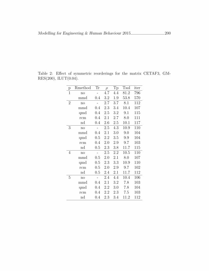
Modelling for Engineering & Human Behaviour 2015 200
Table 2: Effect of symmetric reorderings for the matrix CETAF3, GM-RES(200), ILUT(0.04).
p Rmethod Tr ρ Tp Tsol iter1 no - 4.7 4.4 81.2 796
mmd 0.4 3.2 1.9 53.8 5702 no - 2.7 3.7 8.1 112
mmd 0.4 2.3 3.4 10.4 107qmd 0.4 2.5 3.2 9.1 115rcm 0.4 2.1 2.7 8.0 111nd 0.4 2.6 2.5 10.1 117
3 no - 2.5 4.3 10.9 110mmd 0.4 2.1 3.0 9.0 104qmd 0.5 2.2 3.5 9.9 104rcm 0.4 2.0 2.9 9.7 103nd 0.5 2.3 3.8 11.7 115
4 no - 2.5 2.2 10.5 110mmd 0.5 2.0 2.1 8.0 107qmd 0.5 2.3 3.3 10.9 110rcm 0.5 2.0 2.9 9.7 102nd 0.5 2.4 2.1 11.7 112
5 no - 2.4 4.4 10.4 106mmd 0.4 2.1 3.2 7.8 103qmd 0.4 2.2 3.0 7.8 104rcm 0.4 2.2 2.3 7.5 103nd 0.4 2.3 3.4 11.2 112
Modelling for Engineering & Human Behaviour 2015 201
References
[1] B. Carpentieri. Sparse preconditioners for dense linear systems, fromelectromagnetic applications. PhD thesis, PhD Thesis, l’Institut Na-tional Polytechnique de Toulouse, CERFACS, 2002.
[2] W. C. Chew, J.-M. Jin, E. Michielssen, and J. Song. Fast and EfficientAlgorithms in Computational Electromagnetics and Elastic Waves. Mor-gan & Claypool Publishers, 2009.
[3] I. S. Duff, A. M. Erisman, and J. K. Reid. Direct Methods for SparseMatrices. Oxford University Press, London, 1986.
[4] A. George and J. W. H. Liu. Computer Solution of Large Sparse PositiveDefinite Systems. Prentice-Hall, Englewood Cliffs, NJ., 1981.
[5] M. J. Grote and T. Huckle. Parallel preconditioning with sparse ap-proximate inverses. SIAM J. on Scientific Computing, 18(3):838–853,1997.
[6] G. Karypis and V. Kumar. METIS: A software package for partitioningunstructured graphs, partitioning meshes, and computing fill-reducingorderings of sparse matrices (version 3.0). Technical report, University ofMinnesota, Department of Computer Science and Army HPC ResearchCenter, October 1997.
[7] J. C. Maxwell.. A dynamical theory of the electromagnetic field.155:459–512, 1865.
[8] S. M. Rao, D. R. Wilton, and A. W. Glisson. Electromagnetic scatteringby surfaces of arbitrary shape. IEEE Trans. Antennas Propagat., AP-30:409–418, 1982.
[9] Y. Saad. Iterative Methods for Sparse Linear Systems. PWS PublishingCo., Boston, 1996.
[10] Y. Saad and M. H. Schulz. GMRES: A generalized minimal residualalgorithm for solving nonsymmetric linear systems. SIAM Journal onScientific and Statistical Computing, 7:856–869, 1986.

Numerical Simulation of Needle MovementNozzle Flow Coupled with Spray for a DieselInjector Using an Eulerian Spray Atomization
Model
R. Payri[, J. Gimeno[, P. Martı-Aldaravı[∗, M. Alarcon[
([) CMT - Motores Termicos, Universitat Politecnica de Valencia,
Edificio 6D, Camino de Vera s/n, 46022, Valencia, Spain.
November 30, 2015
1 Introduction
The study of flow characteristics inside Diesel nozzles is tricky due to theirsmall characteristic length and hard testing conditions (very high pressureand velocity). That is the reason why Computational Fluid Dynamics (CFD)is widely used to study such kind of flows [1, 2]. These techniques modelthe real domain generally by finite volume discretization. Therefore, thegeometry of the nozzle must be very well known in advance.
In order to obtain geometrical details of Diesel nozzle, silicone mold tech-nique [3] has been widely used over the years. Nevertheless, new powerfultechniques such as X-ray tomography [4] have been also successfully em-ployed. In fact, this last technique not only allows obtaining the sizing of thenozzle with a resolution of microns, but also the time resolved position of theneedle and measurements in the dense region of the spray [5]. It is knownthat needle movement affect spray behavior (and so combustion efficiency)specially during opening and closing transients [6, 7].
∗e-mail: [email protected]
202
Modelling for Engineering & Human Behaviour 2015 203
From another point of view, the in-nozzle flow pattern defines the spraybehavior and characteristics [8]. Though nozzle flow and spray are clearlylinked. Under this framework, the objective of this work is to employ an al-ready existing Eulerian model, able to simulate nozzle flow and spray at thesame time [10], to computationally address the effects of needle movementon the spray behavior. To do so, Spray A conditions of Engine CombustionNetwork (ECN) [11] are considered. Nozzle of Spray A is very well charac-terized in terms of geometry and flow characteristics, including needle liftmeasurements. However, the time resolution used for measuring needle ve-locity may not be high enough, then it is possible that some post-processing(i.e. moving average) of the experimental signal is required.
2 Methodology
The Eulerian Spray Atomization (ESA) is a homogeneous model built to sim-ulate non-evaporative conditions so far [10], and it has been deeply describedin previous works [10, 12, 13]. In this type of models, the air-fuel mixtureis considered as a single phase and the dispersion is calculated through abalance equation [9].
Simulations (which are peformed in OpenFOAM 2.3.0 R©) set-up is similarto the one configured in previous works [10, 12], being the main differencethe needle position and movement. The needle lift was measured by means ofX-ray tomography [4]. The velocity of the needle has a peaky shape, whichmay lead to unstable or unrealistic simulations, so the signal has been filteredusing a moving average filter. By comparing simulations perfomed with thesetwo needle velocity laws (original and filtered) it is possible to check if thishas an impact on the spray behavior. However, the combination of needlemovement and time varying pressure at inlet boundary leads to mass flowrate curves quite different from experimental ones. Therefore, an additionalsimulation is performed in which the pressure is fixed and the non-filteredneedle velocity is used.
OpenFOAM 2.3.0 R© supports mesh morphing six degree of freedom.However, for this work only the axial movement is needed. Mesh motionis based on solving the cell-center Laplacian for the given component of themotion velocity, and cells are deformed accordingly in all directions to keepcell quality (skewness, aspect ratio) under acceptable levels.
Modelling for Engineering & Human Behaviour 2015 204
3 Results and discussion
First parameters to be analyzed are the mas flow rate and momentum flux,together with the non-dimensional coefficients that define the nature of theflow: Cv, Ca and Cd, following Desantes et al. [14] procedure. All simulationspredict almost the same value for the discharge coefficient Cd, 2% lowerthan the experimental. This is due to the under-prediction of the velocitycoefficient, which means that simulations give a velocity slightly lower thanexperiments. This difference may be related to uncertainties on referencedensity value. Nevertheless, differences are small.
Comparing mass flow rate and momentum flux signals, it can be observedthat time varying pressure inlet boundary by itself is not enough to obtainthe oscillations in mass flow and momentum experimentally observed. Infact, when that condition is combined with needle movement, oscillationsgrow but do not follow experimental data. This means that pressure signalon the rail should not be used as boundary condition in internal nozzle flowsimulations.
Spray parameters need to be also analyzed. Simulation with fixed needleslightly over-estimates the near-field spray penetration, whilst simulationswith moving needle give quite similar curves than experiments. Both sim-ulation curves overlaps, one more evidence that filtering the needle velocitymay not be needed.
4 Conclusions
Spray A conditions have been simulated by using the ESA model. Needlemovement has been taken into account under different approaches: fixedneedle, the raw experimental data for needle lift, and filtered signal to re-move possible instabilities. The following conclusions can be drawn from thecurrent work:
• No clear difference has been observed between raw lift data and thefiltered signal. There is no need of post-processing the needle lift data.Although the acquisition frequency seemed to be low, is enough forperforming simulations.
• Needle movement is needed to capture oscillations experimentally ob-served in mass flow rate and momentum flux. However, it must be
Modelling for Engineering & Human Behaviour 2015 205
combined with the right inlet boundary condition and the proper ini-tialization.
• Errors in spray penetration are minimized if needle movement is con-sidered.
• Spray structure is generally well predicted, except that ESA computa-tional model over-predicts fuel concentration for distances longer than5 mm.
Therefore, when the needle lift is available, it is recommended to con-sider it in the simulations to improve predictions in both nozzle and sprayparameters. Special attention must be paid to inlet boundary condition andinitialization of simulations. Nonetheless, there is still work to do to improveDiesel spray models.
References
[1] F. J. Salvador, J.-V. Romero, M.-D. Rosello and D. Jaramillo, Numer-ical simulation of primary atomization in diesel spray at low injectionpressure, Journal of Computational and Applied Mathematics, In Press,Available on-line, (2015).
[2] G. Strotos, P. Koukpuvinis and A. Theodorakakos, Transient heatingeffects in high pressure Diesel injector nozzles, International Journal ofHeat and Fluid Flow, 51 (2015), pp. 257–267.
[3] V. Macian, V. Bermudez, R. Payri and J. Gimeno, New technique fordetermination of internal geometry of a Diesel nozzle with the use ofsilicone methodology, Experimental Techniques, 39 (2003), pp. 39–43.
[4] A. L. Kastengren, F. Z. Tiloco, C. F. Powell, J. Manin, L. M. Pickett, R.Payri and T. Bazyn, Engine Combustion Network (ECN): Measurementsof Nozzle Geometry and Hydraulic Behavior, Atomization and Sprays,22 (2012), pp. 1011–1052.
[5] A. L. Kastengren, F. Z. Tiloco, D. J. Duke, C. F. Powell, X. Zhangand S. Moon, Time-resolved X-Ray Radiography of Sprays from EngineCombustion Network Spray A Diesel Injectors, Atomization and Sprays,24 (2014), pp. 251–272.
Modelling for Engineering & Human Behaviour 2015 206
[6] W. G. Lee and R. D. Reitz, A Numerical Investigation of Transient Flowand Cavitation within Minisac and VCO Diesel Injector Nozzles, Pro-ceedings of the 2009 Spring Technical Conference of the ASME InternalCombustion Engine Division (2009), pp. 643–653.
[7] R. Payri, J. Gimeno, J. P. Viera and A. H. Plazas, Needle lift profileinfluence on the vapor phase penetration for a prototype diesel directacting piezoelectric injector, Fuel, 113 (2013), pp. 257–265.
[8] V. Bermdez, R. Payri, F. J. Salvador and A. H. Plazas, Study of the in-fluence of nozzle seat type on injection rate and spray behavior, IMechE.Part D: Journal of Automobile Engineering, 219 (2005), pp. 677–689.
[9] A. Vallet, A. A. Burluka and R. Borghi, Development of a EulerianModel for the “Atomization” of a Liquid Jet, Atomization and Sprays,11 (2001), pp. 619–642.
[10] F. J. Salvador, J. Gimeno, J. M. Pastor and P. Martı-Aldaravı, Effectof turbulence model and inlet boundary condition on the Diesel spraybehavior by an Eulerian Spray Atomization (ESA) model, InternationalJournal of Multiphase Flow, 65 (2015), pp. 108-116.
[11] M. Bardi, R. Payri, L. M. Malbec, G. Bruneaux, L. M. Pickett, J. Manin,T. Bazyn and C. Genzale, Engine Combustion Network: Comparison ofSpray Development, Vaporization, and Combustion in Different Com-bustion Vessels, Atomization and Sprays, 22 (2012), pp. 807-842.
[12] J. M. Desantes, R. Payri, J. Gimeno and P. Martı-Aldaravı, Simulationof the First Millimeters of the Diesel Spray by an Eulerian Spray Atom-ization Model Applied on ECN Spray A Injector, SAE Technical Paper2014-01-1418 (2014).
[13] R. Payri, S. Ruiz, J. Gimeno and P. Martı-Aldaravı, Verification of anew CFD compressible segregated and multi-phase solver with differentflux update-equations sequences, Applied Mathematical Modelling, 39(2015), pp. 851–861.
[14] J. M. Desantes, R. Payri, J. M. Pastor and J. Gimeno, Experimentalcharacterization of internal nozzle flow and diesel spray behavior. Part1: Non-evaporative conditions. Atomization and Sprays, 17 (2005), pp.315–345.
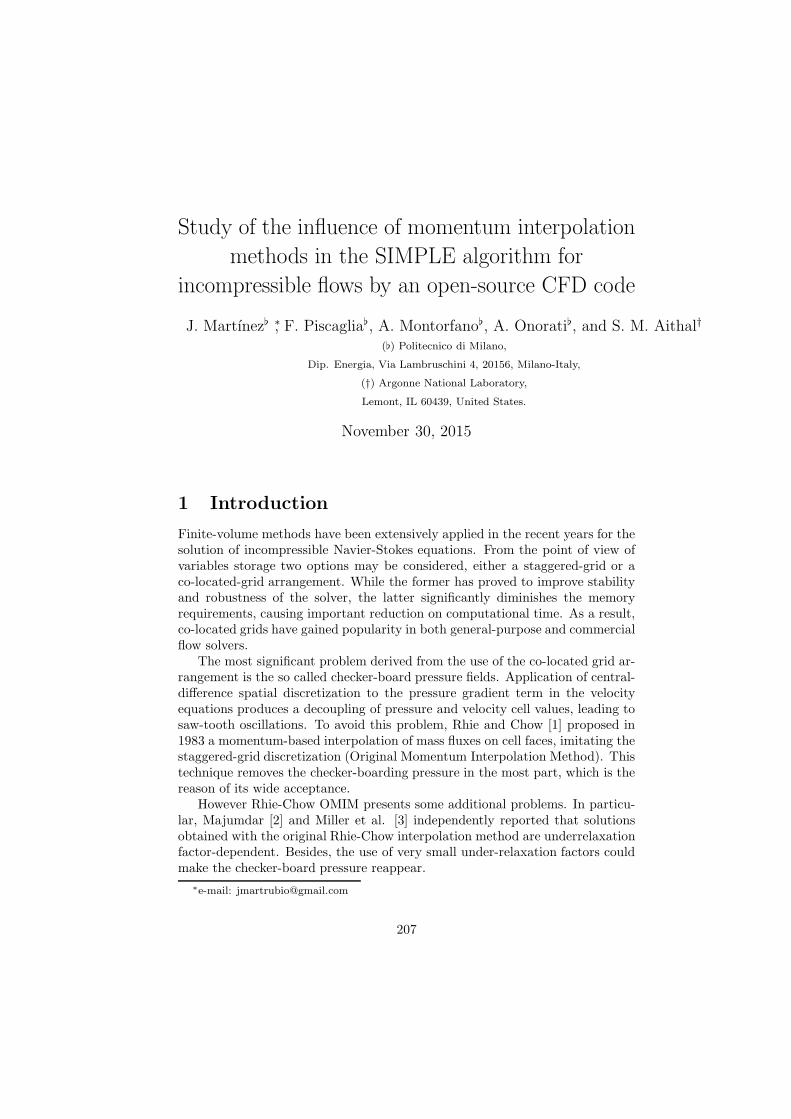
Study of the influence of momentum interpolation
methods in the SIMPLE algorithm for
incompressible flows by an open-source CFD code
J. Martınez ∗, F. Piscaglia, A. Montorfano, A. Onorati, and S. M. Aithal†
() Politecnico di Milano,
Dip. Energia, Via Lambruschini 4, 20156, Milano-Italy,
(†) Argonne National Laboratory,
Lemont, IL 60439, United States.
November 30, 2015
1 Introduction
Finite-volume methods have been extensively applied in the recent years for thesolution of incompressible Navier-Stokes equations. From the point of view ofvariables storage two options may be considered, either a staggered-grid or aco-located-grid arrangement. While the former has proved to improve stabilityand robustness of the solver, the latter significantly diminishes the memoryrequirements, causing important reduction on computational time. As a result,co-located grids have gained popularity in both general-purpose and commercialflow solvers.
The most significant problem derived from the use of the co-located grid ar-rangement is the so called checker-board pressure fields. Application of central-difference spatial discretization to the pressure gradient term in the velocityequations produces a decoupling of pressure and velocity cell values, leading tosaw-tooth oscillations. To avoid this problem, Rhie and Chow [1] proposed in1983 a momentum-based interpolation of mass fluxes on cell faces, imitating thestaggered-grid discretization (Original Momentum Interpolation Method). Thistechnique removes the checker-boarding pressure in the most part, which is thereason of its wide acceptance.
However Rhie-Chow OMIM presents some additional problems. In particu-lar, Majumdar [2] and Miller et al. [3] independently reported that solutionsobtained with the original Rhie-Chow interpolation method are underrelaxationfactor-dependent. Besides, the use of very small under-relaxation factors couldmake the checker-board pressure reappear.
∗e-mail: [email protected]
207

Modelling for Engineering & Human Behaviour 2015 208
In parallel, for the solution of incompressible steady-state flow problems, se-veral algorithms have been proposed during the years, to deal with the pressure-velocity coupling of Navier-Stokes equations. In particular SIMPLE (Semi-Implicit Method for Pressure Linked Equations), SIMPLER (SIMPLE-Revised),SIMPLEC (SIMPLE-Consistent) and PISO (Pressure Implicit with Splitting ofOperators) are some the most well known algorithms.
The aim of the present paper is to apply the method for mass fluxes inter-polation proposed by Majumdar in combination with different pressure-velocitycoupling algorithms, to study the overall solver performance in terms of accuracyof the solution, dependency on the under-relaxation factors and convergencerate. Two simple 2D cases have been selected with this purpose: a laminarlid-driven cavity and a NACA-0012 aifoil profile.
2 Numerical methodology
The open-source finite-volume CFD code OpenFOAM R©, extended with the im-plementation of Majumdar correction and alternative pressure-velocity couplingalgorithms (SIMPLE-R, SIMPLE-C), has been used for this study. The twocases selected for the tests tried to evaluate the performance of the correctionin a theoretical simple laminar case (cavity), where an orthogonal quadrilateralmesh or a triangle mesh with low non-orthogonality was used, and a more com-plex case (airfoil) with a non-orthogonal mesh where turbulence was present andlack of convergence of results might have limited the influence of the correction.For each of the two cases the numerical procedure followed is described below.
2.1 Lid-driven cavity
A laminar lid-driven cavity case was simulated using either a uniform orthogonalmesh, a non-uniform orthogonal mesh or a triangle mesh as shown in Fig. 1.
Figure 1: 2D meshes chosen for cavity case
Two Reynolds numbers, namely 1000 and 5000, were used for the simula-tions. Linear interpolation was used for convective and diffusive terms. Con-vergence was assumed to be achieved when normalized residuals of both com-ponents of velocity and pressure equations was below 1.0 · 10−8. Benchmarksolutions from Ghia et al. [4] have been used to compare vertical velocity pro-files along the horizontal center-line.

Modelling for Engineering & Human Behaviour 2015 209
2.2 NACA 0012 airfoil profile
The turbulent flow (Re ≈ 6 · 106 based on the chord length) around a NACA0012 airfoil profile was studied under incompressible conditions (M = 0.15). Astructured grid of 14625 cells (225 × 65 with 129 points on airfoil surface) wasemployed, giving an approximate average y+ ≈ 1 over the airfoil profile (see Fig.2). Numerical results have been compared to experimental references, includingpressure distribution [5], lift and drag [6] coefficients on upper wall, for differentangles of attack.
Figure 2: 2D mesh of NACA 0012 profile and zoom to airfoil region
3 Results
As expected, the dependency of the solution of OMIM with respect to the veloc-ity under-relaxation is quickly reduced as mesh refinement increases. Majumdarcorrection completely eliminates the dependency, at the cost of reducing the ac-curacy of the solution. It can be proved that Majumdar solution tends to thatobtained by OMIM when velocity under-relaxation factor approaches 0. In fact,if the error in the determination of vertical velocity in one point is plotted withrespect to the number of cells of the simulation (see Fig. 3), we can see howMajumdar solution is completely independent of under-relaxation factors butgenerates always a bigger error than standard OMIM for any value of velocityequations under-relaxation factor.
When comparing the performance of different pressure-velocity coupling al-gorithms, the use of SIMPLE-C significantly reduces the number of iterationsrequired to arrive to a given threshold in the equations residuals, when comparedto other classical algorithms (SIMPLE, SIMPLE-R, PISO) .
Given the slight dependency of results for fine meshes, NACA 0012 wasused to test how important these small variations in velocity profiles affect theprediction of pressure (Cp), drag (CD) and lift coefficient (CL). As shown inFig. 4, for those parameters mainly affected by pressure distribution (Cp, CL)no significant differences are found when OMIM is used for different under-relaxation factors. However, for drag coefficients, where velocity derivativesbecome of importance, some differences might appear. It was checked thatMajumdar correction eliminates most part of these dependencies for the levelor convergence achieved in the simulations.
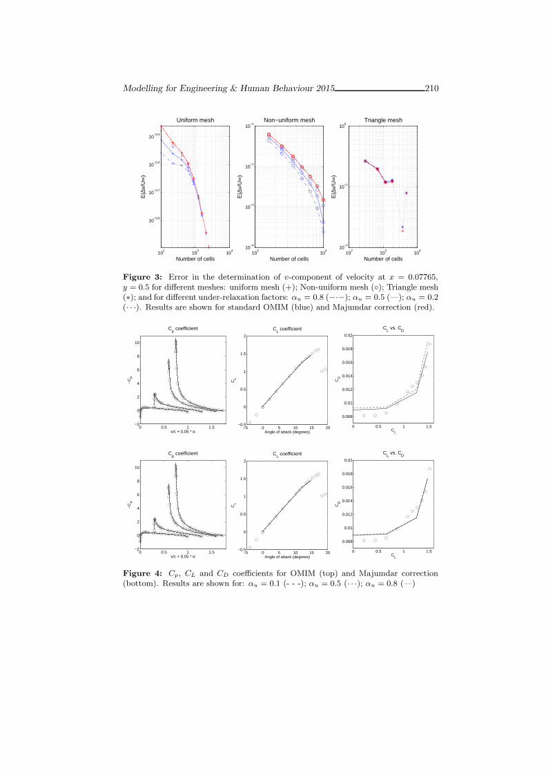
Modelling for Engineering & Human Behaviour 2015 210
102
103
104
10−0.8
10−0.7
10−0.6
10−0.5
Number of cells
E(∆
v/U
∞)
Uniform mesh
103
104
10−4
10−3
10−2
10−1
Number of cells
E(∆
v/U
∞)
Non−uniform mesh
102
103
104
10−2
10−1
100
Number of cells
E(∆
v/U
∞)
Triangle mesh
Figure 3: Error in the determination of v-component of velocity at x = 0.07765,y = 0.5 for different meshes: uniform mesh (+); Non-uniform mesh (); Triangle mesh(∗); and for different under-relaxation factors: αu = 0.8 (−·−); αu = 0.5 (—); αu = 0.2(· · ·). Results are shown for standard OMIM (blue) and Majumdar correction (red).
0 0.5 1 1.5−2
0
2
4
6
8
10
x/c + 0.05 * α
−C
P
Cp coefficient
−5 0 5 10 15 20−0.5
0
0.5
1
1.5
2
CL coefficient
Angle of attack (degrees)
CL
0 0.5 1 1.5
0.008
0.01
0.012
0.014
0.016
0.018
0.02
CL vs. C
D
CL
CD
0 0.5 1 1.5−2
0
2
4
6
8
10
x/c + 0.05 * α
−C
P
Cp coefficient
−5 0 5 10 15 20−0.5
0
0.5
1
1.5
2
CL coefficient
Angle of attack (degrees)
CL
0 0.5 1 1.5
0.008
0.01
0.012
0.014
0.016
0.018
0.02
CL vs. C
D
CL
CD
Figure 4: Cp, CL and CD coefficients for OMIM (top) and Majumdar correction(bottom). Results are shown for: αu = 0.1 (- - -); αu = 0.5 (· · ·); αu = 0.8 (—)

Modelling for Engineering & Human Behaviour 2015 211
4 Conclusions
In the present paper Majumdar correction and two alternative pressure-velocitycoupling algorithms (SIMPLE-C and SIMPLE-R) have been implemented inOpenFOAM R©. Majumdar correction has proved to eliminate the dependencyof the solution on velocity under-relaxation factors. While the dependency ofOMIM is reduced when a fine mesh is used, its influence in coefficients depen-ding on velocity derivatives should still be considered. For the cases studied,SIMPLE-C algorithm has proved to improve the convergence speed with respectto other classical algorithms (SIMPLE, SIMPLE-R or PISO).
References
[1] C.M. Rhie and W. L. Chow. A numerical study of the turbulent flow pastan isolated airfoil with trailing edge separation AIAA J., vol. 21, pp. 1525-1532, 1983
[2] S. Majumdar Role of underrelaxation in momentum interpolation for cal-culation of flow with nonstaggered grids Numerical Heat Transfer, vol. 13,pp. 125-132, 1988
[3] T.F. Miller and F.W. Schmidt Use of a Pressure-Weighted InterpolationMethod for the Solution of Incompressible Navier-Stokes Equations on aNon-Staggered Grid System Numerical Heat Transfer, vol. 14, pp. 213-233,1988
[4] U.Ghia, K. N. Ghia and C. T. Shin High-Re Solutions for IncompressibleFlow using the Navier-Stokes Equation and a Multigrid Method Journal of
Computational Physics, vol. 48, pp. 387-411, 1982
[5] N. Gregory and C. L. O’Reilly Low-Speed Aerodynamic Characteristicsof NACA 0012 Aerofoil Sections, including the Effects of Upper-SurfaceRoughness Simulation Hoar Frost NASA R&M 3726, 1970
[6] C. L. Ladson, A. S. Hill and W. G. Johnson Jr. Pressure Distributionsfrom high Reynolds Number Transonic Tests of a NACA 0012 Airfoil inthe Langley 0.3 Meter Transonic Cryogenic Tunnel NASA TM 100826,1987
Modelling for Engineering & Human Behaviour 2015_________________________________212
Improved railway wheelset-track interaction model
in the high–frequency domain José Martínez-Casas
1, Juan Giner-Navarro
1, F. D. Denia
1, Paloma Vila
1 and L. Baeza
1
1Centro de Investigación en Ingeniería Mecánica, Universitat Politècnica de València,
Camino de Vera s/n, 46022 Valencia, Spain.
e-mail address of corresponding author: [email protected]
ABSTRACT
As it is well known, there are various phenomena related to railway train-track interaction,
some of them caused by the high–frequency dynamics of the system, such as rolling noise,
squeal noise and short-pitch rail corrugation. Due to these phenomena and some others
unsolved so far, a large effort has been made over the last 40 years in order to define suitable
models for studying train-track interaction. In most of the early works the vehicle was modelled
as a rigid body system. Later, the introduction of the wheelset flexibility in the model was
required to have a more realistic representation of the wheel–rail interaction effects at higher
frequencies. Recently, more advanced train-track interaction models have been developed for
vehicle running on straight track and negotiating a curved track, where the rails are modelled by
means of Timoshenko beam elements with cyclic boundary conditions. Thus, the rail model is
valid up to 1.5 kHz for lateral vibration and up to 2 kHz for vertical vibration. Therefore, this
confines the frequency range of validity for the complete train-track model to 1.5 kHz.
The aim of this paper is to propose an improvement of the train-track interaction models so as to
extend their range of validity above 1.5 kHz. With this purpose, a track model based on the 3D
Moving Element Method (MEM) is developed to replace the Timoshenko beam considered in
earlier studies, adopting cyclic boundary conditions and Eulerian coordinates. The MEM
approach considers a mobile finite element (FE) mesh which moves with the vehicle speed, so
the mass of the rail ‘flows’ with the velocity of the vehicle but in the opposite direction through
the mesh. The MEM permits to fix the contact area in the middle of the finitely long track and,
hence, to refine longitudinally the mesh only around the contact area. This Eulerian-modal
approach reduces substantially the number of degrees of freedom of the problem whereby,
together with a refinement just around the fixed contact area, the computational cost of the
proposed model is much lower than FEM models widely used. Simulation results for the
proposed modelling approach are presented and discussed for different excitation sources
including random rail roughness and singularities such as wheel flats. All the simulation cases
are made for a Timoshenko beam and a 3D MEM rail models, in order to point out the
differences in the contact forces above the range of validity of the Timoshenko beam.
1. INTRODUCTION
The complexity of the train-track interaction comes from the vibration coupling between the
railway vehicle and a flexible track, in which wheel–rail contact forces couple both sub-systems
and their surface imperfections, such as rail roughness and wheel out-of-roundness, excite the
global system. Unwanted phenomena such as damage of the rolling surfaces in the form of high
levels of noise and vibration [1], corrugation [2], rolling contact fatigue [3] and dynamic
stresses may appear in some cases due to large level of vibration and large dynamic fluctuations
of the contact forces, which need to be carefully considered in order to avoid failures due to
metal fatigue.

Modelling for Engineering & Human Behaviour 2015_________________________________213
Accordingly, many suitable train-track interaction models have been developed over the last 40
years. Finite Element (FE) models have strongly entered in railways research to extend the
frequency range above 1 kHz to address the previous phenomena, but only very recently,
further works have considered the flexibility and inertial effects due to wheelset rotation [4]. In
order to widen the range of valid frequencies, this wheelset model is used in this paper, which
takes into account the gyroscopic and inertial effects associated with the rotation by using
Eulerian modal coordinates and, hence, reducing the computational cost.
In recently published train-track interaction models, the rails are modelled by means of
Timoshenko beam elements with cyclic boundary conditions [5], thus the rail model being
valid up to 1.5 kHz for lateral vibration and up to 2 kHz for vertical vibration according to [1];
this confines the frequency range of validity for the complete train-track model to 1.5 kHz. The
aim of this paper is, hence, to propose an improvement of the train-track interaction model [4]
so as to extend their range of validity above 1.5 kHz. With this purpose, a track model based on
the Moving Element Method (MEM) technique is developed to replace the Timoshenko beam
considered in earlier studies, adopting cyclic boundary conditions and Eulerian coordinates.
The proposed model is based on the Moving Element Method (MEM) presented by Koh et. al.
[6, 7] for 1D and 2D beam tracks. In the present work, this Eulerian approach has been extended
to a straight 3D real track extruded from the UIC-60 profile (3D MEM model). The Eulerian
coordinate system is attached to the moving vehicle instead of a fixed coordinate system.
Hence, the mesh is moving with this mobile frame and consequently the material of the rail
‘flows’ into this mesh. This relative motion requires considering the material derivative for the
formulation of the rail dynamics. In this model, the contact area is fixed on the same elements,
allowing refine the mesh just around the fixed contact area. Therefore, the 3D MEM model
permits to decrease the computational cost compared to the FEM models commonly employed.
Results for the proposed modelling approach are presented and discussed for a selected vehicle
type and a straight track for different excitation sources including random rail roughness and
singularities such as wheel flats. All the simulation cases are made for a Timoshenko beam and
a 3D MEM models representing the track. The vertical contact force for both model are
analysed and compared with special attention to discrepancies above the range of validity of the
Timoshenko beam (from 1.5 to 8.5 kHz).
2. THE VEHICLE–TRACK INTERACTION MODEL
For the vehicle-track interaction model, a sub-structuring technique [5] is followed in this
paper, permitting to divide the whole system into three substructures: the vehicle, the rails and
the discrete rail supports, all coupled by the wheel-rail contact forces and the forces generated
at the rail pads. The vehicle is confined to one wheelset with primary suspension, and two static
forces on the primary suspensions are included to represent the weight of the bogie and the car
body. The wheelset has been modelled as a flexible and rotating wheelset [4], in which
Eulerian-modal coordinates are employed due to the axial symmetry of the body. This modal
approach leads to a significant reduction of the computation cost of the simulation.
In the present paper, the track is included by two different flexible models: Timoshenko beam
model [5], with a limited frequency range of validity (up to 1.5 kHz for lateral vibration and up
to 2 kHz for vertical vibration), and the 3D Moving Element Method (MEM) proposed in this
work with the purpose of extending the range to the high-frequency domain. A cyclic approach
is considered in both cases since it provides some benefit with respect to classical track
modelling or the finite one.
Modelling for Engineering & Human Behaviour 2015_________________________________214
For the wheel-rail contact forces in the contact patch, Hertzian model is adopted here for the
normal contact and FASTSIM is the software used for the tangential contact that depends on the
normal contact force and of the creepages. The contact model considers the real geometry of the
contacting profiles and includes the non-linearities between creepages and creep forces The
discrete rail supports are introduces in the form of lumped parameter systems, where the rail
pads are modelled as lumped viscoelastic elements, sleepers as lumped masses, and the ballasts
as equivalent stiffness and damping below the lumped masses.
3. 3D MOVING ELEMENT METHOD (MEM)
The Moving Element Method (MEM) was presented first by Koh et. al. [6, 7] as an efficient
Eulerian approach to treat moving loads applied on finite beams. This section summarise the
effort of extending this technique to a 3D finite track with cyclic boundary conditions at the
edges aiming to widen the frequency range of validity of the Timoshenko beam model used in
previous works. Taking into account the material derivative and convective terms, and using
the virtual work principle and modal superposition, the equation of motion is obtained below:
QqAKqCqM ~~~
2~ 2VV , (1)
where V is the velocity of the vehicle, q is the Eulerian-modal coordinate vector, Q is the
vector of generalised forces from contact and rail pad forces, and the matrices are the following:
dVol
~ TΦΦM , d
xVol
~ T
ΦΦC , d
xxVol
~
T
ΦΦA , (2)
being Φ the mode shape functions matrix of the cyclic rail, M~
the modal mass matrix, K~
the
modal stiffness matrix, C~
introduces the inertial force due to the convective velocity, and
A~
contains the inertial force due to the convective acceleration.
The modal differential equation of motion of the rail in Eq. (1) is linear and then the matrices
are only calculated one time at the beginning of the simulation. Therefore, the proposed 3D
MEM model is suitable in the high–frequency domain and has a low computational cost.
4. RESULTS
In this section, results of wheelset-track interaction simulations for the proposed modelling
approach are presented considering different sources of excitation: random rail roughness and
wheelflat. All the simulations consider the vehicle running at 300 km/h through a tangent track;
each case is run separately for a Timoshenko beam and a 3D MEM modelling the track. Both
models are compared by the vertical contact force obtained from the simulations above the
range of validity of the Timoshenko beam (from 1.5 to 8.5 kHz) in order to study the
contributions of the 3D MEM in the high–frequency range.
Fig. 1 shows the time history of the vertical contact force for an excitation caused by randomly
corrugated rails, assuming a corrugation spectrum corresponding to the ISO 3095 limit, which
establishes a third-octave band spectrum of the rail roughness. As expected, the dynamic
fluctuations of the vertical contact force show a complex waveform, arising from the dynamic
response of the wheelset-track system to broadband random excitation. The results for both
track models present a similar trend and mean values, although a higher frequency content is
observed for the MEM.
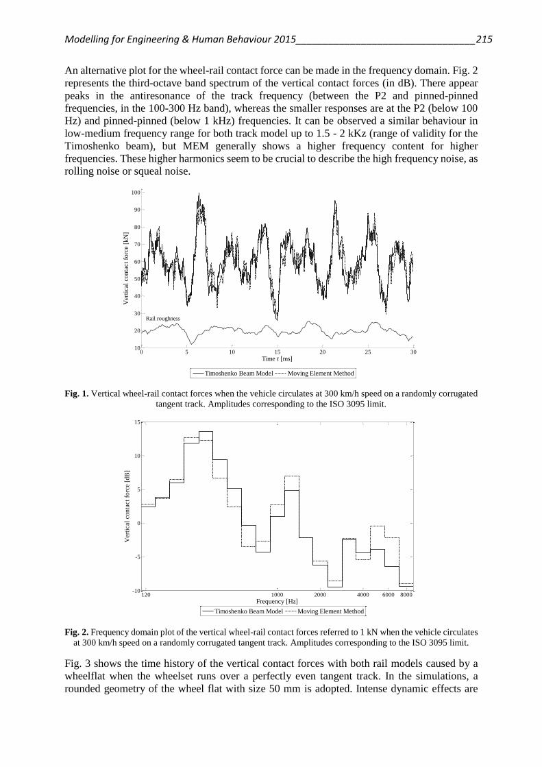
Modelling for Engineering & Human Behaviour 2015_________________________________215
An alternative plot for the wheel-rail contact force can be made in the frequency domain. Fig. 2
represents the third-octave band spectrum of the vertical contact forces (in dB). There appear
peaks in the antiresonance of the track frequency (between the P2 and pinned-pinned
frequencies, in the 100-300 Hz band), whereas the smaller responses are at the P2 (below 100
Hz) and pinned-pinned (below 1 kHz) frequencies. It can be observed a similar behaviour in
low-medium frequency range for both track model up to 1.5 - 2 kKz (range of validity for the
Timoshenko beam), but MEM generally shows a higher frequency content for higher
frequencies. These higher harmonics seem to be crucial to describe the high frequency noise, as
rolling noise or squeal noise.
0 5 10 15 20 25 3010
20
30
40
50
60
70
80
90
100
Rail roughness
Time t [ms]
Vert
ical
conta
ct
forc
e [
kN
]
Timoshenko Beam Model Moving Element Method
Fig. 1. Vertical wheel-rail contact forces when the vehicle circulates at 300 km/h speed on a randomly corrugated
tangent track. Amplitudes corresponding to the ISO 3095 limit.
120 1000 2000 4000 6000 8000-10
-5
0
5
10
15
Frequency [Hz]
Vert
ical
conta
ct
forc
e [
dB
]
Timoshenko Beam Model Moving Element Method
Fig. 2. Frequency domain plot of the vertical wheel-rail contact forces referred to 1 kN when the vehicle circulates
at 300 km/h speed on a randomly corrugated tangent track. Amplitudes corresponding to the ISO 3095 limit.
Fig. 3 shows the time history of the vertical contact forces with both rail models caused by a
wheelflat when the wheelset runs over a perfectly even tangent track. In the simulations, a
rounded geometry of the wheel flat with size 50 mm is adopted. Intense dynamic effects are
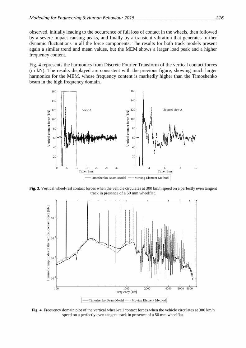
Modelling for Engineering & Human Behaviour 2015_________________________________216
observed, initially leading to the occurrence of full loss of contact in the wheels, then followed
by a severe impact causing peaks, and finally by a transient vibration that generates further
dynamic fluctuations in all the force components. The results for both track models present
again a similar trend and mean values, but the MEM shows a larger load peak and a higher
frequency content.
Fig. 4 represents the harmonics from Discrete Fourier Transform of the vertical contact forces
(in kN). The results displayed are consistent with the previous figure, showing much larger
harmonics for the MEM, whose frequency content is markedly higher than the Timoshenko
beam in the high frequency domain.
0 5 10 15 20 25 300
20
40
60
80
100
120
140
160
Time t [ms]
Vert
ical
co
nta
ct
forc
e [
kN
]
View A
Timoshenko Beam Model Moving Element Method
4 6 8 100
20
40
60
80
100
120
140
160
Time t [ms]
Vert
ical
co
nta
ct
forc
e [
kN
] Zoomed view A
Fig. 3. Vertical wheel-rail contact forces when the vehicle circulates at 300 km/h speed on a perfectly even tangent
track in presence of a 50 mm wheelflat.
100 1000 2000 4000 6000 8000
10-4
10-3
10-2
10-1
Frequency [Hz]
Har
monic
am
pli
tudes
of
the
ver
tica
l co
nta
ct f
orc
e [k
N]
Timoshenko Beam Model Moving Element Method
Fig. 4. Frequency domain plot of the vertical wheel-rail contact forces when the vehicle circulates at 300 km/h
speed on a perfectly even tangent track in presence of a 50 mm wheelflat.

Modelling for Engineering & Human Behaviour 2015_________________________________217
5. CONCLUSIONS
This paper has presented a new 3D model for a finite railway track which has been formulated
through the Moving Element Method (MEM) technique and developed as a Finite Element
(FE) model in order to improve the modelling of high frequency dynamics. The model
considers an Eulerian coordinate system attached to the moving vehicle instead of a fixed
coordinate system and adopts cyclic boundary conditions. This approach permits to decrease
the computational cost compared to the FEM models commonly used.
Results for the vertical contact force are presented for two types of excitation: randomly
corrugated tangent track and excitation arising from a wheelflat when the wheelset running at
300 km/h along. The MEM and Timoshenko beam models have been compared in all cases.
Both models show a similar behaviour in the low-medium frequency domain (up to 2 kHz) for
two excitation cases, where a similar trend and mean values can be observed. Significant
discrepancies appear, however, in the high frequency range, above 2-3 kHz, where the MEM
model has higher frequency content and larger peaks than Timoshenko beam. Hence, the
proposed MEM model seems suitable to describe the high frequency dynamics associated to
different railway phenomena such as short pitch rail corrugation, wheelflat excitation, axle
fatigue, rolling noise, squeal noise and braking noise.
ACKNOWLEDGEMENTS
The authors gratefully acknowledge the financial support of Ministerio de Economía y
Competitividad and the European Regional Development Fund (project
TRA2013-45596-C2-1-R), as well as Generalitat Valenciana (project Prometeo/2012/023) and
Ministerio de Educación, Cultura y Deporte (project SP20140659) as part of Programa Campus
de Excelencia Internacional.
REFERENCES
[1] D. J. Thompson, Railway Noise and Vibration: Mechanisms, Modelling and Means of
Control, Elsevier, 2009.
[2] J. C. O. Nielsen, R. Lundén, A. Johansson and T. Vernersson, Train-track Interaction and
Mechanisms of Irregular Wear on Wheel and Rail Surfaces, Vehicle System Dynamics 40 (1-3)
(2003) 3-54.
[3] A. Ekberg, Fatigue of railway wheels, The Wheel/Rail Interface Handbook Woodhead
Publishing in Mechanical Engineering (2009) 211-244.
[4] J. Martínez-Casas, L. Mazzola, L. Baeza and S. Bruni, Numerical estimation of stresses in
railway axles using a train-track interaction model, International Journal of Fatigue 47 (2013)
18-30.
[5] L. Baeza and H. Ouyang, A railway track dynamics model based on modal substructuring
and a cyclic boundary condition, Journal of Sound and Vibration 330 (2011) 75–86.
[6] C. G. Koh, J. S. Y. Ong, D. K. H. Chua and J. Feng, Moving Element Method for train-track
dynamics, International Journal for Numerical Methods in Engineering 56 (2003) 1549–1567.
[7] C. G. Koh, G. H. Chiew, C. C. Lim, A numerical method for moving load on continuum,
Journal of Sound and Vibration 300 (2007) 126–138.
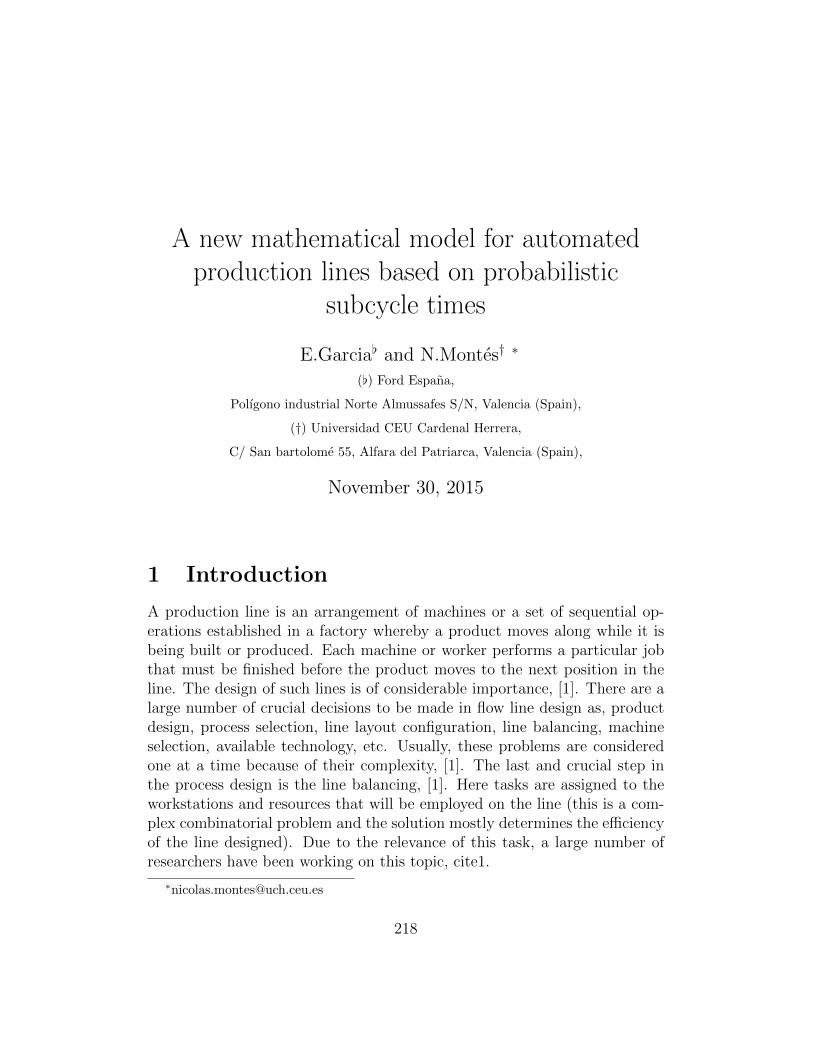
A new mathematical model for automatedproduction lines based on probabilistic
subcycle times
E.Garcia[ and N.Montes† ∗
([) Ford Espana,
Polıgono industrial Norte Almussafes S/N, Valencia (Spain),
(†) Universidad CEU Cardenal Herrera,
C/ San bartolome 55, Alfara del Patriarca, Valencia (Spain),
November 30, 2015
1 Introduction
A production line is an arrangement of machines or a set of sequential op-erations established in a factory whereby a product moves along while it isbeing built or produced. Each machine or worker performs a particular jobthat must be finished before the product moves to the next position in theline. The design of such lines is of considerable importance, [1]. There are alarge number of crucial decisions to be made in flow line design as, productdesign, process selection, line layout configuration, line balancing, machineselection, available technology, etc. Usually, these problems are consideredone at a time because of their complexity, [1]. The last and crucial step inthe process design is the line balancing, [1]. Here tasks are assigned to theworkstations and resources that will be employed on the line (this is a com-plex combinatorial problem and the solution mostly determines the efficiencyof the line designed). Due to the relevance of this task, a large number ofresearchers have been working on this topic, cite1.
218

Modelling for Engineering & Human Behaviour 2015 219
But, what happens when the line is designed and installed in the factory?.The designers defined the maximum production rate, mainly in jobs per hour(JPH), knowing as Engineering Running Capacity (ERC). The goal of thefactory employees is to achieve this maximum production rate, defining thethroughput of the line. Reality shows that the ERC is extremely difficult orimpossible to achieve so the factory employees define a new based-experiencemaximum production rate and is known as the Engineering Running Rate(ERR). The literature does not offer a reason about this throughput reduc-tion, being the objective of the present paper.
Therefore, in the present paper a novel mathematical model that willallow us to demonstrate that the ERR is due to the machine variability partsis developed . The proposed model is tested in a real welding line in Ford S.A.located at the Almussafes factory. This line has 35 welding units distributedin 8 workstations. The paper is organized as follows. Section 2 presentsa mathematical model. Section 3 presents the mini-terms characterization.Section 4 presents a a real welding line and the simulation results. Section 5concludes the paper with an emphasis on future research challenges.
2 Mathematical model. From micro-term to
long term
The literature classifies the data used in the analysis into long-term andshort-term. Long-term is mainly used for process planning, while short-termfocuses primarily on process control. Therefore, following the definition in[2], the short-term is referred to an operational period not large enough fora machines failure period to be described by a statistic distribution. Themachine’s cycle time is considered short-term. The present study redefinesshort-term into two new terms, mini-term and micro-term. A mini-termcould be defined as a machine part, in a preventive maintenance policy or ina breakdown, where it could be replaced in an easier and faster manner thananother machine part subdivision. Also a mini-term could be defined as asubdivision that allows us to understand and study the machine behavior. Inthe same way, a micro-term is defined as each mini-term part that could bedivided itself. In general, Factory Plan time can be represented as a tensor;
F =∑16l6p
∑16s6k
∑16M6j
∑16m6i
= τl,s,M,m (1)
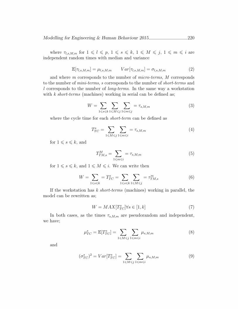
Modelling for Engineering & Human Behaviour 2015 220
where τl,s,M,m for 1 6 l 6 p, 1 6 s 6 k, 1 6 M 6 j, 1 6 m 6 i areindependent random times with median and variance
E[τl,s,M,m] = µl,s,M,m V ar[τl,s,M,m] = σl,s,M,m (2)
and where m corresponds to the number of micro-terms, M correspondsto the number of mini-terms, s corresponds to the number of short-terms andl corresponds to the number of long-terms. In the same way a workstationwith k short-terms (machines) working in serial can be defined as;
W =∑16s6k
∑16M6j
∑16m6j
= τs,M,m (3)
where the cycle time for each short-term can be defined as
T sTC =
∑16M6j
∑16m6i
= τs,M,m (4)
for 1 6 s 6 k, and
TMTM,s =
∑16m6i
= τs,M,m (5)
for 1 6 s 6 k, and 1 6M 6 i. We can write then
W =∑16s6k
= T sTC =
∑16s6k
∑16M6j
= τmTM,s (6)
If the workstation has k short-terms (machines) working in parallel, themodel can be rewritten as;
W = MAX[T sTC ]∀s ∈ [1, k] (7)
In both cases, as the times τs,M,m are pseudorandom and independent,we have;
µsTC = E[T s
TC ] =∑
16M6j
∑16m6i
µs,M,m (8)
and
(σsTC)2 = V ar[T s
TC ] =∑
16M6j
∑16m6i
µs,M,m (9)
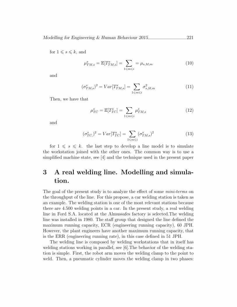
Modelling for Engineering & Human Behaviour 2015 221
for 1 6 s 6 k, and
µsTM,s = E[T s
TM,s] =∑
16m6i
= µs,M,m (10)
and
(σsTM,s)
2 = V ar[T sTM,s] =
∑16m6i
σ2s,M,m (11)
Then, we have that
µsTC = E[T s
TC ] =∑
16m6i
µsTM,s (12)
and
(σsTC,)
2 = V ar[T sTC ] =
∑16m6i
(σsTM,s)
2 (13)
for 1 6 s 6 k. the last step to develop a line model is to simulatethe workstation joined with the other ones. The common way is to use asimplified machine state, see [4] and the technique used in the present paper
3 A real welding line. Modelling and simula-
tion.
The goal of the present study is to analyze the effect of some mini-terms onthe throughput of the line. For this propose, a car welding station is taken asan example. The welding station is one of the most relevant stations becausethere are 4.500 welding points in a car. In the present study, a real weldingline in Ford S.A. located at the Almussafes factory is selected.The weldingline was installed in 1980. The staff group that designed the line defined themaximum running capacity, ECR (engineering running capacity), 60 JPH.However, the plant engineers have another maximum running capacity, thatis the ERR (engineering running rate), in this case defined in 51 JPH.
The welding line is composed by welding workstations that in itself haswelding stations working in parallel, see [6].The behavior of the welding sta-tion is simple. First, the robot arm moves the welding clamp to the point toweld. Then, a pneumatic cylinder moves the welding clamp in two phases:
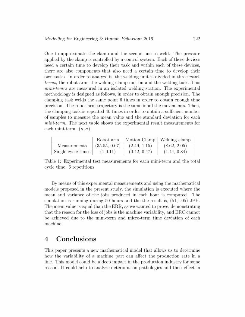
Modelling for Engineering & Human Behaviour 2015 222
One to approximate the clamp and the second one to weld. The pressureapplied by the clamp is controlled by a control system. Each of these devicesneed a certain time to develop their task and within each of these devices,there are also components that also need a certain time to develop theirown tasks. In order to analyze it, the welding unit is divided in three mini-terms, the robot arm, the welding clamp motion and the welding task. Thismini-temrs are measured in an isolated welding station. The experimentalmethodology is designed as follows, in order to obtain enough precision. Theclamping task welds the same point 6 times in order to obtain enough timeprecision. The robot arm trajectory is the same in all the movements. Then,the clamping task is repeated 40 times in order to obtain a sufficient numberof samples to measure the mean value and the standard deviation for eachmini-term. The next table shows the experimental result measurements foreach mini-term. (µ, σ).
Robot arm Motion Clamp Welding clampMeasurements (35.55, 0.67) (2.49, 1.15) (8.62, 2.05)
Single cycle times (1,0.11) (0.42, 0.47) (1.44, 0.84)
Table 1: Experimental test measurements for each mini-term and the totalcycle time. 6 repetitions
By means of this experimental measurements and using the mathematicalmodels proposed in the present study, the simulation is executed where themean and variance of the jobs produced in each hour is computed. Thesimulation is running during 50 hours and the the result is, (51,1.05) JPH.The mean value is equal than the ERR, as we wanted to prove, demonstratingthat the reason for the loss of jobs is the machine variability, and ERC cannotbe achieved due to the mini-term and micro-term time deviation of eachmachine.
4 Conclusions
This paper presents a new mathematical model that allows us to determinehow the variability of a machine part can affect the production rate in aline. This model could be a deep impact in the production industry for somereason. It could help to analyze deterioration pathologies and their effect in

Modelling for Engineering & Human Behaviour 2015 223
the throughput. In this sense, a deep characterization of the machine partdeterioration is required. Although, manufactures have a threshold for thelifespan of the parts, however, for maintenance workers the evolution of thedeterioration during the lifespan time could be crucial in the throughput ofthe line, as well as for the detection of pathologies with great variability.
5 Acknowledgments
Authors wish to thank Ford Espana S.A and in particular Almussafes Factoryfor their support in the present research.
References
[1] O.Battaıa and A.Dolghi. A taxonomy of line balancing problems andtheir solution approaches. International Journal of production Eco-nomics, Volume(142):259–277, 2013.
[2] PhD Q. Chang. Supervisory factory control based on real-time produc-tion feedback, 2011.
[3] L.Li, Q.Chang, J.Ni. Real time production improvement throughbottleneck control. International Journal of production research,Volume(47:21):6145–6158, 2009.
[4] F.Leal, R.F.S.Costa, J.A.B.Montevechi, D.A.Almeida, F.A.S.Marins Apractical guide for operational validation of discrete simulation modelspesquisa Operational, Volume(31(1)):57–77, 2011.
[5] PhD C.E.Lopez. Unbalanced workload allocation in large assembly lines,2014.
[6] PhD E. Garcia. Analisis de los sub-tiempos de ciclo tecnico en la mejoradel rendimiento de las lıneas de fabricacion, Summer 2016.
Mathematical Model and Implementation ofRational Processing
H. Mora[ ∗, J. Mora Pascual[, J.M. Garcıa Chamizo[
and M.T. Signes Pont[
([) Specialized Processors Architecture Laboratory
Department of Computer Technology, University of Alicante
San Vicent del Raspeig, Alicante (E-03080). Spain
November 30, 2015
1 Introduction
High precision computing is a very active research area due to the numberof interesting applications that need it.
This work aims to propose a mathematical model to represent and op-erate rational numbers without error. This model constitutes the formalframework of an arithmetic architecture where computational techniques aredefined to build the operators with rational numbers.
The key idea of this research is based on representing explicitly the non-zero periodic part of the rational number expressed by the positional numbersystem. The main challenge of this notation is to develop arithmetic methodsto compute the numbers, especially if they are also represented in floatingpoint.
∗e-mail: [email protected]
224
Modelling for Engineering & Human Behaviour 2015 225
2 Related Work
There are several alternatives to represent binary and decimal numbers in acomputer [2,3] and even some proposals allow to represent rational numberswithout error [4]. The standard representation formats [1] are not amongthem.
The main drawbacks of the more accurate ways of representing numbersare the complexity of their arithmetic methods and the lack of precision whenthe numbers are transformed into positional number system expressions.
The most recent proposals based on the interval arithmetic and on-line[5] methods offer alternatives of interest which improve the precision of theresults. However, they are unable to provide an exact value but only anapproximation for irrational or periodic rational numbers.
3 Formal Framework for High Precision Com-
puting
Let f be a general mathematical function. Any computable function whoseresult approximates to f according to a particular implementation is definedimplementation function of f. In this way:
codomain(Γf (~x)) ⊆ codomain(f(~x)) (1)
and then,
∀~x ∈ domain(Γf (~x)), |Γf (~x)− f(~x)| ≤ ε (2)
where,~x : function argumentsε : Approximation of f by Γ.
An architecture Λ is characterised both by the set of functions that it pro-vides and by the way in which they are implemented. Let the following setof functions be:
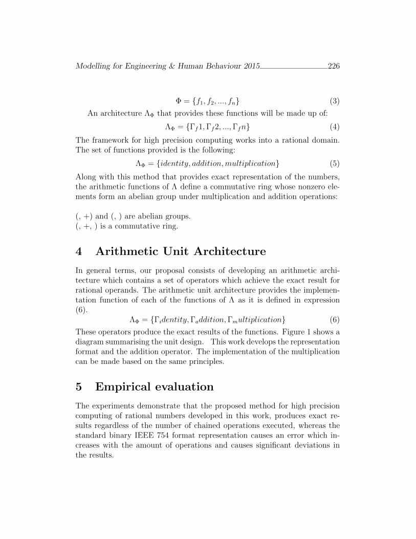
Modelling for Engineering & Human Behaviour 2015 226
Φ = f1, f2, ..., fn (3)
An architecture ΛΦ that provides these functions will be made up of:
ΛΦ = Γf1,Γf2, ...,Γfn (4)
The framework for high precision computing works into a rational domain.The set of functions provided is the following:
ΛΦ = identity, addition,multiplication (5)
Along with this method that provides exact representation of the numbers,the arithmetic functions of Λ define a commutative ring whose nonzero ele-ments form an abelian group under multiplication and addition operations:
(, +) and (, ) are abelian groups.(, +, ) is a commutative ring.
4 Arithmetic Unit Architecture
In general terms, our proposal consists of developing an arithmetic archi-tecture which contains a set of operators which achieve the exact result forrational operands. The arithmetic unit architecture provides the implemen-tation function of each of the functions of Λ as it is defined in expression(6).
ΛΦ = Γidentity,Γaddition,Γmultiplication (6)
These operators produce the exact results of the functions. Figure 1 shows adiagram summarising the unit design. This work develops the representationformat and the addition operator. The implementation of the multiplicationcan be made based on the same principles.
5 Empirical evaluation
The experiments demonstrate that the proposed method for high precisioncomputing of rational numbers developed in this work, produces exact re-sults regardless of the number of chained operations executed, whereas thestandard binary IEEE 754 format representation causes an error which in-creases with the amount of operations and causes significant deviations inthe results.
Modelling for Engineering & Human Behaviour 2015 227
Figure 1: General overview of the Rational Arithmetic Architecture
6 Conclusions
The research presented in this paper describes a mathematical model forrepresenting and processing rational numbers. This proposal is an alternativecalculation model when the accuracy in storage and processing of rationalnumbers is a key aspect to be considered.
References
[1] ANSI/IEEE. IEEE Standard for Binary Floating-Point Arithmetic.ANSI/IEEE Standard 754-2008 IEEE, 2008.
[2] JL. Sanchez et al. An iterative method for improving decimalcalculations on computers Mathematical and Computer Modelling,Volume(50):869–878, 2009.
[3] A. Vazquez, E. Antelo A High-Performance Significand BCD Adderwith IEEE 754-2008 Decimal Rounding IEEE Symposium on ComputerArithmetic, 135–144, 2009.
[4] D. Piso and J.D. Bruguera. Obtaining Accurate Error Expressions andBounds for Floating-Point Multiplicative Algorithms The ComputerJournal, Volume(2):319–331, 2014.
[5] C. Garca, S. Gonzalez, J. Villalba, E.L. Zapata On-line DecimalAdder with RBCD Representation IEEE International Conference onApplication-Specific Systems, Architectures and Processors, 53–60, 2012.
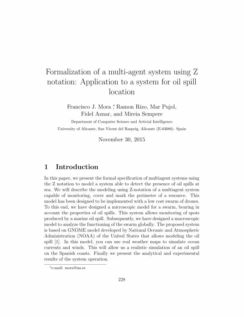
Formalization of a multi-agent system using Znotation: Application to a system for oil spill
location
Francisco J. Mora ∗, Ramon Rizo, Mar Pujol,Fidel Aznar, and Mireia Sempere
Department of Computer Science and Articial Intelligence
University of Alicante, San Vicent del Raspeig, Alicante (E-03080). Spain
November 30, 2015
1 Introduction
In this paper, we present the formal specification of multiagent systems usingthe Z notation to model a system able to detect the presence of oil spills atsea. We will describe the modeling using Z-notation of a multiagent systemcapable of monitoring, cover and mark the perimeter of a resource. Thismodel has been designed to be implemented with a low cost swarm of drones.To this end, we have designed a microscopic model for a swarm, bearing inaccount the properties of oil spills. This system allows monitoring of spotsproduced by a marine oil spill. Subsequently, we have designed a macroscopicmodel to analyze the functioning of the swarm globally. The proposed systemis based on GNOME model developed by National Oceanic and AtmosphericAdministration (NOAA) of the United States that allows modeling the oilspill [1]. In this model, you can use real weather maps to simulate oceancurrents and winds. This will allow us a realistic simulation of an oil spillon the Spanish coasts. Finally we present the analytical and experimentalresults of the system operation.
∗e-mail: [email protected]
228

Modelling for Engineering & Human Behaviour 2015 229
2 Formalization with Z language
The language Z is accessible to researchers from variety of different back-grounds and allows us to provide a consistent unified formal account of anabstract agent system. Precisely and unambiguously provide meanings forthe common concepts. Allows formally define system modeling and sys-tem behavior. Well-structured to provide a foundation for subsequent de-velopment of increasingly more refined concepts. ZMichael Luck and Markd’Inverno wrote Structuring a Z Specification to Provide a Formal Frameworkfor Autonomous Agent Systems in 1995 [2].
The main components of the model are environment, objects, agentsand autonomous agents. An agent is an instantiation of an object togetherwith an associated goal or set of goals.For objects, agents and autonomousagents we define their state when situated in an environment in ObjectState,AgentState and AutonomousAgentState. We define how they act in an envi-ronment in the schemes ObjectAction, AgentAction and AutonomousAgen-tAction respectively. For agents and autonomous agents, we detail how theyperceive in a given environment in AgentPerception and AutonomousAgent-Perception.
We will modeled a system to mark and cover a oil spills, defining thedifferent schemes.
3 Microscopic System Behavior
We propose a homogeneous behavior that run in all the agents of the swarm.This behavior has three states: Wander, Resource and InResource. In broadterms, the agents initially sought by the environment trying to find sometrace of the spill. Once the spill is detected, the agent is directed towardsit. Finally it will try to keep inside (to cover) or on its perimeter (to mark)depending on the desired behavior. When agents are inside the spill andtherefore do not perceive their limit, they do a random motion until it meetsthe sea.
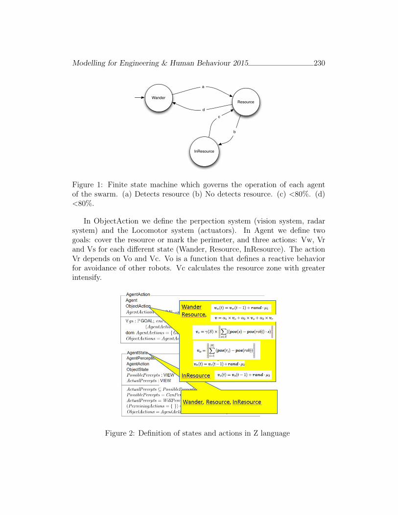
Modelling for Engineering & Human Behaviour 2015 230
WanderResource
InResource
c
b
d
a
Figure 1: Finite state machine which governs the operation of each agentof the swarm. (a) Detects resource (b) No detects resource. (c) <80%. (d)<80%.
In ObjectAction we define the perpection system (vision system, radarsystem) and the Locomotor system (actuators). In Agent we define twogoals: cover the resource or mark the perimeter, and three actions: Vw, Vrand Vs for each different state (Wander, Resource, InResource). The actionVr depends on Vo and Vc. Vo is a function that defines a reactive behaviorfor avoidance of other robots. Vc calculates the resource zone with greaterintensify.
Figure 2: Definition of states and actions in Z language
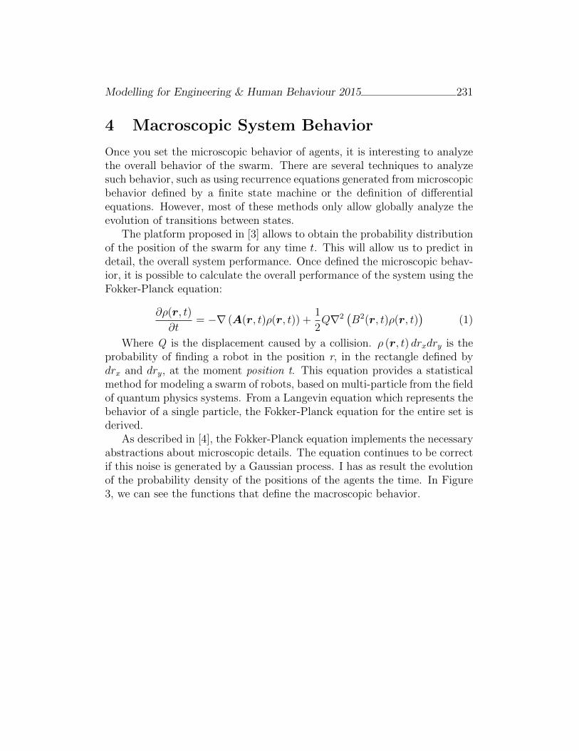
Modelling for Engineering & Human Behaviour 2015 231
4 Macroscopic System Behavior
Once you set the microscopic behavior of agents, it is interesting to analyzethe overall behavior of the swarm. There are several techniques to analyzesuch behavior, such as using recurrence equations generated from microscopicbehavior defined by a finite state machine or the definition of differentialequations. However, most of these methods only allow globally analyze theevolution of transitions between states.
The platform proposed in [3] allows to obtain the probability distributionof the position of the swarm for any time t. This will allow us to predict indetail, the overall system performance. Once defined the microscopic behav-ior, it is possible to calculate the overall performance of the system using theFokker-Planck equation:
∂ρ(r, t)
∂t= −∇ (A(r, t)ρ(r, t)) +
1
2Q∇2
(B2(r, t)ρ(r, t)
)(1)
Where Q is the displacement caused by a collision. ρ (r, t) drxdry is theprobability of finding a robot in the position r, in the rectangle defined bydrx and dry, at the moment position t. This equation provides a statisticalmethod for modeling a swarm of robots, based on multi-particle from the fieldof quantum physics systems. From a Langevin equation which represents thebehavior of a single particle, the Fokker-Planck equation for the entire set isderived.
As described in [4], the Fokker-Planck equation implements the necessaryabstractions about microscopic details. The equation continues to be correctif this noise is generated by a Gaussian process. I has as result the evolutionof the probability density of the positions of the agents the time. In Figure3, we can see the functions that define the macroscopic behavior.
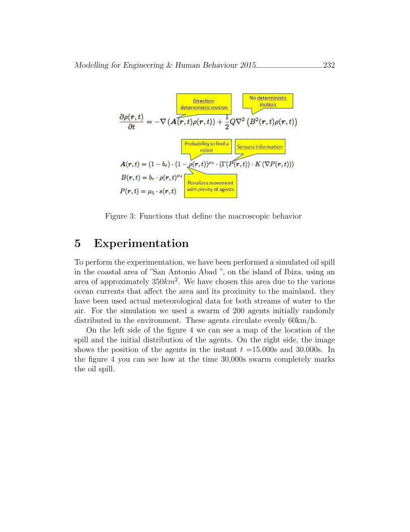
Modelling for Engineering & Human Behaviour 2015 232
Figure 3: Functions that define the macroscopic behavior
5 Experimentation
To perform the experimentation, we have been performed a simulated oil spillin the coastal area of ”San Antonio Abad ”, on the island of Ibiza, using anarea of approximately 350km2. We have chosen this area due to the variousocean currents that affect the area and its proximity to the mainland. theyhave been used actual meteorological data for both streams of water to theair. For the simulation we used a swarm of 200 agents initially randomlydistributed in the environment. These agents circulate evenly 60km/h.
On the left side of the figure 4 we can see a map of the location of thespill and the initial distribution of the agents. On the right side, the imageshows the position of the agents in the instant t =15.000s and 30.000s. Inthe figure 4 you can see how at the time 30,000s swarm completely marksthe oil spill.
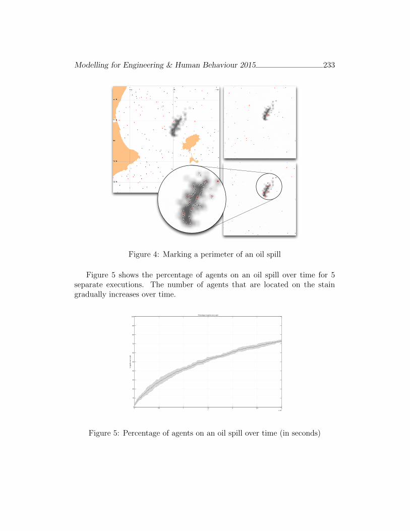
Modelling for Engineering & Human Behaviour 2015 233
Figure 4: Marking a perimeter of an oil spill
Figure 5 shows the percentage of agents on an oil spill over time for 5separate executions. The number of agents that are located on the staingradually increases over time.
0 0.5 1 1.5 2 2.5 3x 10⁴
0
10
20
30
40
50
60
70
80
90
100Percentage of agents over a spill
t
% A
gent
s ov
er a
spi
ll
Figure 5: Percentage of agents on an oil spill over time (in seconds)
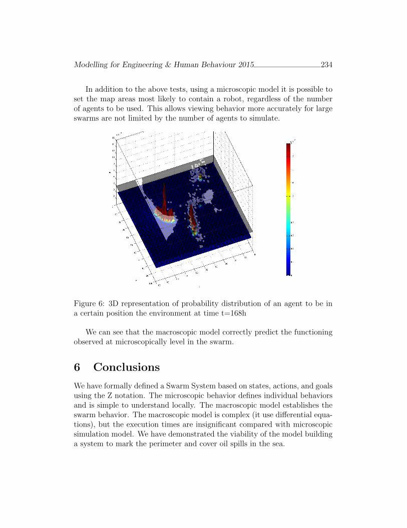
Modelling for Engineering & Human Behaviour 2015 234
In addition to the above tests, using a microscopic model it is possible toset the map areas most likely to contain a robot, regardless of the numberof agents to be used. This allows viewing behavior more accurately for largeswarms are not limited by the number of agents to simulate.
Figure 6: 3D representation of probability distribution of an agent to be ina certain position the environment at time t=168h
We can see that the macroscopic model correctly predict the functioningobserved at microscopically level in the swarm.
6 Conclusions
We have formally defined a Swarm System based on states, actions, and goalsusing the Z notation. The microscopic behavior defines individual behaviorsand is simple to understand locally. The macroscopic model establishes theswarm behavior. The macroscopic model is complex (it use differential equa-tions), but the execution times are insignificant compared with microscopicsimulation model. We have demonstrated the viability of the model buildinga system to mark the perimeter and cover oil spills in the sea.

Modelling for Engineering & Human Behaviour 2015 235
References
[1] United States. National Ocean Service. Office of Response and Restora-tion. General noaa operational modelling environment (gnome technicaldocumentation. U.S. Dept. of commerce, National Oceanic and Atmo-spheric Administration, National Ocean Service, Office of Response andRestoration, 2012
[2] Justin Clark and Rafael Fierro. Mobile robotic sensors for perimeterdetection and tracking. ISA Transactions, 46(1):3-13, 2007
[3] Hamann, Heiko and Worn, Heinz. A framework of space–time continu-ous models for algorithm design in swarm robotics. Swarm Intelligence.Spinger. 2008 pag.209-239
[4] Hamann, Heiko. Space-Time Continuous Models of Swarm Robotic Sys-tems: Supporting Global-to-Local Programming. Springer.2010
Acknowledgement
This work has been supported by the Spanish Ministerio de Economıa yCompetitividad project TIN2013-40982-R. Project co-financed with FEDERfunds.
An algorithm for trajectory semantic similarity
Francisco Moreno[ ∗, Santiago Roman†, and Vania Bogorny‡
([ †) Universidad Nacional de Colombia, Sede Medellın.,
Carrera 80 No 65-223 - Nucleo Robledo Medellın, Colombia,
(‡) Universidad Federal de Santa Catarina,
CEP 88040-900 - Campus Universitario Cx.P.476 Florianpolis S.C.
November 30, 2015
1 Introduction
Trajectory data are collected as raw trajectories, represented as a sequenceof space time points, that correspond to the position (x, y) of an object ina space at an instant (t). The discovery of similar movement behavior fromtrajectory data is interesting for several domains, such as trajectory cluster-ing and nearest neighbor queries. In this extended abstract, we propose anew similarity function for semantic trajectories, which supports both the se-mantics of the places visited by the trajectories and the activities performedat each place, what to the best of our knowledge has not been addressed be-fore. While previous works [1, 2] do only consider the exact matching of thesemantic dimension, we propose to use a taxonomy of places and activitiesto consider partial matching of places and activities performed at a place.The main contribution of this work is a new similarity function for measuringdifferent semantic information of trajectory data.
∗e-mail: [email protected]
236
Modelling for Engineering & Human Behaviour 2015 237
2 Trajectories similarity
Similarly to [3] we consider a Category (concept) Tree for the Classificationof the Sites (CTCS). For simplicity, each site is associated with a uniquecategory corresponding to a leaf node of the tree. Similarly, we consider aCategory Tree for the Classification of the Activities (CTCA).Let S be a set of m sites S = s1, s2, . . . , sm where si = (s id, s name,s cat), where s id is the site identifier, s name its name and s cat representsthe CTCS category (leaf node) which is associated with the site. Thus, onesite is (directly) associated with one leaf node of the CTCS and (indirectly)with all the ancestor nodes of that leaf node in the CTCS.Example. Let S = s1, s2, s3, s4, s5, s6, s7 where s1 = (1, Cinema Central,Cinema), s2 = (2, Bocagrande, Beach), s3 = (3, Universidad de Carta-gena, University), s4 = (4, El Rosario, Beach), s5 = (5, Golden Disco,Discotheque), s6 = (6, Universidad de Bolvar, University), and s7 = (7,Botanical Garden, Park).Similarly, we define a set of p activities A = a1, a2, . . . , ap where ai =(a id, a name, a cat), where a id is the identifier of the activity, a name itsname and a cat represents the CTCA category (leaf node) which is associatedwith the activity.Example. LetA = a1, a2, a3, a4, a5, a6, a7, a8 where a1 = (1, Studying math,studying), a2 = (2, Bicycling, Playing sports), a3 = (3, Reading sciencefiction, Reading), a4 = (4, Dancing electronic, Dancing), a5 = (5, StudyingSpanish, Studying), a6 = (6, Swimming, Playing sports), a7 = (7, Singingrock, Karaoke) and a8 = (8, Watching adventure movies, watching movies).On the other hand, a trajectory T is a set of n episodes T = e1, e2, . . . , en,where ei = (si, ai, ti):si ∈ S represents the site where the episode occurred,ai ∈ A represents the activity accomplished in the site si,ti = (tini, tfin) represents the time of start (tini) and end (tfin) ot theepisode, tini < tfin.
Example. Let T1 = e1, e2, e3, e4 where e1 = (s6, a5, t1), e2 = (s4, a6, t2),e3 = (s1, a8, t3), and e4 = (s7, a3, t4); and where t1 = (8am, 12m), t2 =(3pm, 4pm), t3 = (4pm, 5 : 30pm), and t4 = (8pm, 9pm), all times correspondto 18/Feb/2015. .To calculate the similarity we extend the proposal of [4]. They propose aformula to determine whether two trajectories are spatial similarity completebased on the set of points of interest (POI) of each one and a threshold θ.
Modelling for Engineering & Human Behaviour 2015 238
Let POIns,Tithe set of all associated sites (either directly or indirectly) with
one node ns ∈ CTCS included in the episodes of trajectory Ti. The similaritybetween two trajectories Ti and Tj with regard to ns, Cns,Ti,Tj
, is calculatedby Equation (1).
Cns,Ti,Tj=
∣∣POIns,Ti∩ POIns,Tj
∣∣∣∣POIns,Ti∪ POIns,Tj
∣∣ (1)
That is, Cns,Ti,Tjis the relationship between the total number of sites common
to the two trajectories associated with the node ns and the total number ofsites of the two trajectories associated with that node. Cns,Ti,Tj
= INDEF(undefined) if POIns,Ti
∪POIns,Tj6= ∅, i.e., when none of the two trajectories
have sites associated with the node ns.Consider two trajectories Ti and Tj. In our method, we compute the similar-ity of each node ns ∈ CTCS (or ns ∈ CTCA if the similarity is consideredwith regard to activities) by Equation (1), i.e., SIMns = Cns,Ti,Tj
. In thisway, the user can analyze the trajectories similarity with regard to eachCTCS node. For instance, if ns is the root of CTCS, then Cns,Ti,Tj
indicatesthe similarity of the trajectories from a general point of view (node “Site”).The user can then analyze the similarity from a more specific point of view ashe descends through the levels of CTCS or a CTCA (a “drill-down”). Notethat in our method, to calculate the similarity of a non-leaf node, calculatingthe similarity of its child nodes, is not required.
References
[1] Josh Jia-Ching Ying, Eric Hsueh-Chan Lu, Wang-Chien Lee, Tz-ChiaoWeng, and Vincent S Tseng. Mining user similarity from semantic tra-jectories. In Proceedings of the 2nd ACM SIGSPATIAL InternationalWorkshop on Location Based Social Networks, pages 19–26. ACM, 2010.
[2] Vania Bogorny, Chiara Renso, Artur Ribeiro Aquino, FernandoLucca Siqueira, and Luis Otavio Alvares. Constant–a conceptual datamodel for semantic trajectories of moving objects. Transactions in GIS,18(1):66–88, 2014.
[3] Min-Joong Lee and Chin-Wan Chung. A user similarity calculation basedon the location for social network services. In Database Systems for Ad-vanced Applications, pages 38–52. Springer, 2011.

Modelling for Engineering & Human Behaviour 2015 239
[4] Hongbin Zhao, Qilong Han, Haiwei Pan, and Guisheng Yin. Spatio-temporal similarity measure for trajectories on road networks. In In-ternet Computing for Science and Engineering (ICICSE), 2009 FourthInternational Conference on, pages 189–193. IEEE, 2009.
Capturing the Subjacent Risk of Death from a Population: theWavelet Approximation
I. Baeza Sampere ∗ and F. Morillas Jurado †
Universitat de Valencia,
Dpt. Economia Aplicada, Avgda. Tarongers s/n, 46122, Valencia (Spain).
November 30, 2015
1 IntroductionIn the study of the biometric behavior of a population it is usual to analyze some biometrics characteristics:life expectancy, risk of death (or survival) at age x, and others. This work focuses in the study of the risk ofdeath at each age x. It is relevant to remark that the value of the risk of death it is unknown (generally).
In this work a method based in the wavelet decomposition with multiresolution schema, combiningapproximation by Thresholding and Piecewise Polynomial Harmonic (PPH) techniques is articulated toestimate a subjacent risk of death of a population.
It is important to emphasize (for the demographic and actuarial fields) the importance that has to obtaingood estimates of the true probabilities of death. The estimation of the subjacent risk can be used toestimate the premiums of several types of insurance policies; or the mathematics reserves (obligatory) thatan insurance company must set aside; or to estimate the Sustainability Factor to determine the age of theretirement, or the quantity of the pensions (in the spanish case) (view [14]). In this context, the instrumentwidely used to summarize the experience of mortality observed in a region or period is the Life Table ([2]).This construction it is organized by age, and the information that we can find corresponds to the calledbiometric functions. Among these functions, the most commons are: the number of exposed at risk ofdying at age x,lx; the number of death at age x, dx; the crude rates of death at age x, qx; the life expectancyat several ages, eωx ; and others.
In particular, the study of the age of death is easier if we consider that the variable is continuous and weassume that there is a real rate but it is altered by random fluctuations. From this, this work considers thatthis phenomenon has a random nature and that it is impossible to replicate. This fact makes that the valuesof biometric functions are always unknown and that only estimations can be obtained. Then, the efforts ofthis study it is in making estimates of the underlying values of qx, x = 0, . . . , ω ( ω being the highestage considered in the study) . We perceive the sum of both (real rates and random fluctuations) and weassume that true rates have a structural behavior. This hypothesis justifies the extensive development of thegraduation techniques.
∗e-mail:[email protected]†e-mail:[email protected]
240
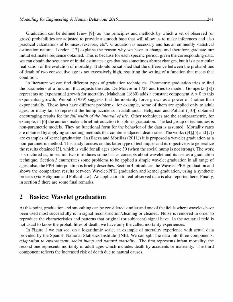
Modelling for Engineering & Human Behaviour 2015 241
Graduation can be defined (view [9]) as "the principles and methods by which a set of observed (orgross) probabilities are adjusted to provide a smooth base that will allow us to make inferences and alsopractical calculations of bonuses, reserves, etc". Graduation is necessary and has an eminently statisticalestimation nature. London [12] explains the reason why we have to change and therefore graduate ourinitial estimates sequence obtained. This is because for each specific period, given the corresponding data,we can obtain the sequence of initial estimates ages that has sometimes abrupt changes, but it is a particularrealization of the evolution of mortality. It should be satisfied that the difference between the probabilitiesof death of two consecutive age is not excessively high, requiring the setting of a function that meets thatcondition.
In literature we can find different types of graduation techniques. Parametric graduation tries to findthe parameters of a function that adjusts the rate: De Moivre in 1724 and tries to model. Gompertz ([8])represents an exponential growth for mortality; Makeham (1860) adds a constant component A > 0 to thisexponential growth; Weibull (1939) suggests that the mortality force grows as a power of t rather thanexponentially. These laws have different problems: for example, some of them are applied only to adultages; or many fail to represent the hump accidents in adulthood. Heligman and Pollard ([10]) obtainedencouraging results for the full width of the interval of life. Other techniques are the semiparametric, forexample, in [6] the authors make a brief introduction to splines graduation. The last group of techniques isnon-parametric models. They no functional form for the behavior of the data is assumed. Mortality ratesare obtained by applying smoothing methods that combine adjacent death rates. The works ([4],[5] and [7])are examples of kernel graduation. In (Baeza and Morillas (2011)) it is proposed a wavelet graduation as anon-parametric method. This study focuses on this latter type of techniques and its objective is to generalizethe results obtained [3], which is valid for all ages above 30 (when the social hump is not strong). The workis structured as, in section two introduces some basics concepts about wavelet and its use as a graduationtechnique. Section 3 enumerates some problems to be applied a simple wavelet graduation in all range ofages; also, the PPH interpolation is briefly describes. Section 4 introduces the Wavelet-PPH graduation andshows the comparison results between Wavelet-PPH graduation and kernel graduation, using a syntheticprocess (via Heligman and Pollard law). An application to real-observed data is also reported here. Finally,in section 5 there are some final remarks.
2 Basics: Wavelet graduationAt this point, graduation and smoothing can be considered similar and one of the fields where wavelets havebeen used most successfully is in signal reconstruction/cleaning or cleaned. Noise is removed in order toreproduce the characteristics and patterns that original (or subjacent) signal have. In the actuarial field isnot usual to know the probabilities of death, we have only the called mortality experiences.
In Figure 1 we can see, on a logarithmic scale, an example of mortality experience with actual dataprovided by the Spanish National Statistics Institute (INE). We can split the data into three components:adaptation to environment, social hump and natural mortality. The first represents infant mortality, thesecond one represents mortality in adult ages which includes death by accidents or maternity. The thirdcomponent reflects the increased risk of death due to natural causes.
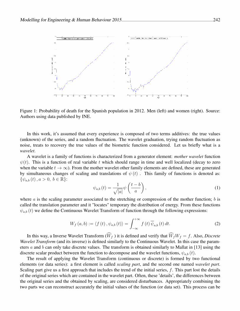
Modelling for Engineering & Human Behaviour 2015 242
Figure 1: Probability of death for the Spanish population in 2012. Men (left) and women (right). Source:Authors using data published by INE.
In this work, it’s assumed that every experience is composed of two terms additives: the true values(unknown) of the series, and a random fluctuation. The wavelet graduation, trying random fluctuation asnoise, treats to recovery the true values of the biometric function considered. Let us briefly what is awavelet.
A wavelet is a family of functions is characterized from a generator element: mother wavelet functionψ(t). This is a function of real variable t which should range in time and well localized (decay to zerowhen the variable t→∞). From the mother wavelet other family elements are defined, these are generatedby simultaneous changes of scaling and translations of ψ (t) . This family of functions is denoted as:ψa,b (t) , a > 0, b ∈ R:
ψa,b (t) =1√|a|ψ
(t− ba
), (1)
where a is the scaling parameter associated to the stretching or compression of the mother function; b iscalled the translation parameter and it "locates" temporary the distribution of energy. From these functionsψa,b (t) we define the Continuous Wavelet Transform of function through the following expressions:
Wf (a, b) := 〈f (t) , ψa,b (t)〉 =
∫ +∞
−∞f (t)ψa,b (t) dt. (2)
In this way, a Inverse Wavelet Transform (Wf ) it is defined and verify that WfWf = f . Also, DiscreteWavelet Transform (and its inverse) is defined similarly to the Continuous Wavelet. In this case the param-eters a and b can only take discrete values. The transform is obtained similarly to Mallat in [13] using thediscrete scalar product between the function to decompose and the wavelet functions, ψa,b (t).
The result of applying the Wavelet Transform (continuous or discrete) is formed by two functionalelements (or data series): a first element is called scaling part, and the second one named wavelet part.Scaling part give us a first approach that includes the trend of the initial series, f . This part lost the detailsof the original series which are contained in the wavelet part. Often, these ’details’, the differences betweenthe original series and the obtained by scaling, are considered disturbances. Appropriately combining thetwo parts we can reconstruct accurately the initial values of the function (or data set). This process can be
Modelling for Engineering & Human Behaviour 2015 243
applied iteratively and application leads: on another scale, a new part scaling and wavelet and so on. Ifthe process only is applied in the scaling part, it is named Multiresolution Analysis; if, also, it is appliedin the wavelet part, it is named Wavelets Packets. Often, the wavelet part and the scaling part obtained areorthogonal, so is, the information contained in a part is not contained in the other, i.e., the information it iscomplementary, not redundant. It is usual, for example in signal processing, to assume that when a seriesof data has random fluctuations (noise or not), these are in the wavelet part. So the elimination or reductionof noise is linked to the treatment of wavelet part (as previous to apply inverse transform to recoverythe signal). The aim of the wavelet graduation is to reduce or even eliminate random fluctuations usingthresholding techniques: truncating the values of wavelet part, assuming certain threshold as an elementthat determines whether a value is or not considered as random fluctuation.
3 Limitations of the simple wavelet graduation: The PPH interpola-tion
The wavelet graduation may have more or less significant drawbacks according to the available informationor the functional relationship of the data. In the case of life tables, in [3], this technique only can beapplied to ranges above 30 years of age. For younger age mortality curve has a non-linear relationship thatcomplicates the analysis by the lack of information. We consider important to highlight some aspects:
• When we apply the wavelet technique, the incorporation of symmetric information at the ends of theseries introduces noise discontinuity.
• The problem of discontinuity reappears if we use a wavelet family with a big support or if we useMultiresolution Analysis.
• Some effect, similar to the Gibbs phenomenon, has also been detected by smoothing the central area,the accident or social hump.
To avoid these limitations we consider the PPH interpolation as a previous step to applied the wavelet grad-uation, increasing synthetically the available data. The PPH technique is a nonlinear interpolation schemeof forth order and depending of the data. It was introduced in [1] and based on a piecewise polynomialharmonic operator. The PPH interpolation has several desirable features:
• Each polynomial piece is constructed with four centered point,
• On smooth region it is as accurate as its linear equivalent,
• No introduce oscillations and
• Preserve the concavity / convexity of the function.
The PPH polynomial value at is given by the expression:
Pj
(xj+ 1
2
)=fj + fj+1
2− 1
4Dh2 (3)
where
D =
2DjDj+1
Dj+Dj+1if DjDj+1 > 0
0 otherwise.(4)
and Dj = f [xj−1, xj, xj+1] are the divided differences associates to the interpolatory stencil.
Modelling for Engineering & Human Behaviour 2015 244
4 Combining wavelet and PPH techniques to graduate:validationAs we have seen, graduation wavelet has problems when we apply it to the entire range of age of thebiometric function. To solve this we will introduce some additional information for inter annual data.These new data will be given by the PPH interpolation since it allows incorporating additional data withoutintroducing oscillations and preserving the concavity (or convexity) of the function.
The calibration and validation of the Wavelet-PPH technique that we proposed, it is do measuring thecapacity of the recovery the true probabilities of death. In the practice this probabilities are unknown,for this reason we articulate a synthetic procedure, which give us an arbitrary number of synthetic deathexperiences (N = 104), all of them equally plausible from the same -and known- true probabilities ofdeath(via Helligman and Pollard law,HPL). The numeric procedure it is based on the HPL to obtain a (true)probabilities of death, and estimates the synthetics values of the next variables: number of deaths for eachage,dx; and the exposed at risk of death lx. The relation between them and the numerical procedure are,for each age x = 0, 1, . . . , ω: dx ∼ Bi(lx, qx), dx = lx − lx+1, with initial value l0 = 105 (arbitrary).Briefly, to obtain a first synthetic scenario: (i) the initial value of l0 is fixed in all experiment, 104.(ii) Itis obtained d10 as a random number from Bi(l0, q0). (iii) The number of exposed at risk to age x = 1 isestimated as survival at age 0 via l11 = l0 − d10. (iv) The synthetic observed rates is q10 =
d10l0
. (v) Nextly, we
iterate the process for next age, so is: d11 ∼ Bi(l11, q1); l12 = l11 − d11; and q11 =d11l11
. The procedure continuefor x = 2, . . . , ω; obtaining the first sequence of synthetic observed rates q10, q
11, . . . , q
1ω. To obtain the
others synthetic observed rates, the procedure it is initialized obtaining alternative values for each variablesdkx, l
kx and qkx, for k = 1, 2, . . . , N . The procedure described ability us to measue The simulation procedure
allows us to apply the graduation method to each series of synthetic values,qk0 , qk1 , . . . , q
kω, k = 1, . . . , N , and
enables us to measure the capacity of the recover the true values (prefixed via HPL). Also, these syntheticseries are used to compare the Wavelet-PPH technique with Gaussian kernel graduation. We consider twotypes of indicators: goodness of fit and smoothness:
The Mean relative indicator (IRM): IRM (q) = 1ω+1
ω∑x=0
|qx−qx|qx
.
The Mean squared relative indicator (IRCM): IRCM (q) = 1ω+1
ω∑x=0
|qx−qx|2qx
.
The Whittaker-Henderson smoothness indicator [15]: S = |S (qx)− S (qx)|where S (qx) =ω−2∑x=0
(∆2qx)2
In the above definitions qx denotes the theoretical probability of death (HPL), and qx indicates thegraduated probability, the value obtained by applying the graduation to each generated realizations. Thedefined indicators suggest that the lower value is the best estimate of the theoretical probability is obtained,suggesting that another technical improvement in this regard.
Table 1 shows the results of the comparison between the Wavelet-PPH graduation and the Gaussiankernel graduation. In columns 3 and 4 we can see the mean value of the indicators for the 104 syntheticdeath experiences. The last column presents the percentage of times that Wavelet-PPH obtains better resultsthan Gaussian kernel graduation.

Modelling for Engineering & Human Behaviour 2015 245
Table 1. Indicators. Comparison Wavelet-PPH vs. Kernel
N Indicator Wavelet-PPH Kernel Better W-PPH(%)IRM 0,0338977 0,03903211 86,74
100 IRCM 0,00370256 0,00885898 99,84S 0,00058177 0,00945352 100,00
IRM 0,034489398 0,0392806 85,37200 IRCM 0,003280213 0,009398363 100,00
S 0,000700086 0,009761079 100,00IRM 0,034557725 0,039082103 82,74
400 IRCM 0,003582433 0,009322405 99,96S 0,000870859 0,00998631 100,00
IRM 0,035888371 0,038810222 74,07800 IRCM 0,00369508 0,009175132 99,97
S 0,002292422 0,010123821 100,00
The table 2 shows the parameters for the Wavelet-PPH graduation. We opted for the biorthogonalwavelet family. Wavelet is selected by means of a criterion based on energy retention instead an exhaustivestrategy like in [3]. The measure is given by H = ‖qx‖2
‖qx‖2. We work with a criterion for thresholding based
on [13].
Table 2. Parameters used in Wavelet-PPH technique
N Wavelet Scales Thresholding100 Biorthogonal 3.3 2 0,15200 Biorthogonal 3.3 3 0,2400 Biorthogonal 3.3 4 0,25800 Biorthogonal 3.3 5 0,3
In Figure 2 (left), are presented for the entire range of ages: the Heligman and Pollard theorical model; arandom realization; and the two approximations by graduation, the kernel graduation and the Wavelet-PPHgraduation (with N=400 and the parameters given by table 2). In Figure 2(right) we observe details of thesefunctions more closely.
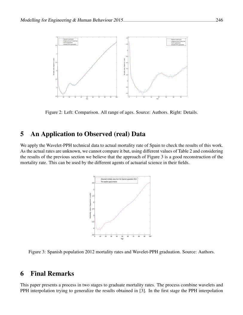
Modelling for Engineering & Human Behaviour 2015 246
0 5 10 15 20 25 30 35
-3.4
-3.2
-3
-2.8
-2.6
-2.4
-2.2
-2
-1.8
-1.6
Age
Mort
alit
y r
ate
s (
logaritm
ic s
cale
)
Random realization
Heligmand and Pollard law
Kernel graduation
Wavelet-PPH graduation
0 10 20 30 40 50 60 70 80 90 100-3.5
-3
-2.5
-2
-1.5
-1
-0.5
0
Age
Mort
alit
y r
ate
s (
logaritm
ic s
cale
)
Random realization
Heligmand and Pollard law
Kernel graduation
Wavelet-PPH graduation
Figure 2: Left: Comparison. All range of ages. Source: Authors. Right: Details.
5 An Application to Observed (real) DataWe apply the Wavelet-PPH technical data to actual mortality rate of Spain to check the results of this work.As the actual rates are unknown, we cannot compare it but, using different values of Table 2 and consideringthe results of the previous section we believe that the approach of Figure 3 is a good reconstruction of themortality rate. This can be used by the different agents of actuarial science in their fields.
0 10 20 30 40 50 60 70 80 90 100-4.5
-4
-3.5
-3
-2.5
-2
-1.5
-1
-0.5
0
Age
Mort
ality
rate
s (
logaritm
ic s
cale
)
Spanish population 2012 mortality rates and wavelet graduation
Observed mortality rates from the Spanish population 2012
The wavelet approximation
Figure 3: Spanish population 2012 mortality rates and Wavelet-PPH graduation. Source: Authors.
6 Final RemarksThis paper presents a process in two stages to graduate mortality rates. The process combine wavelets andPPH interpolation trying to generalize the results obtained in [3]. In the first stage the PPH interpolation
Modelling for Engineering & Human Behaviour 2015 247
allows to incorporate additional data without introducing oscillations and preserving the concavity (or con-vexity) of the function. The second stage use wavelets eliminate the noise (or random fluctuations) in orderto reconstruct the true values of the biometric function considered. That technique can be applied to allrange of ages and, in the sense of the indicators used, give us better results than kernel graduation. Also, thetechnique presented is more robust in the sense that, when the indicator considered is better (minus value)for the kernel graduation than Wavelet-PPH technique, the relative difference is higher than if we considerthe reverse relation.
AcknowledgementsThis research was partially supported by Ministerio de Economía y Competitividad under grant MTM2012-31698.
References[1] Amat S., Busquier S. and Candela V. A polynomial approach to the piecewise hyperbolic method. I.J. Comput. Fluid
Dynam.,3(17): 205–217, 2003.
[2] Ayuso M., Corrales H., Guillen M., Pérez-Marín A.M. and Rojo J.L. Estadistica Actuarial Vida. Barcelona: UBe, 2007.
[3] Baeza I. and Morillas F.G. Using wavelet to non-parametric graduation of mortalily rates Anales del Instituto de ActuariosEspañoles, 17: 135–164,2011.
[4] Copas J. and Haberman S. Non parametric graduation using kernel methods Journal of the Institute of Actuaries, (110):135–156, 1983.
[5] Felipe A., Guillen M., Nielsen J. Longevity studies based on kernel hazard estimation. Insurance: Mathematics andEconomics, (28):191–204,2001.
[6] Forfar D.,McCutcheon J. and Wilkie A. On graduation by mathematical formulae Journal of the Institute of Actuaries,(115): 693–694,1988.
[7] Gavin J.,Haberman S. and Verrall R. Moving weighted average graduation using kernel estimation Mathematics andEconomics, 12 (2):113–126, 1993.
[8] Gompertz B. On the nature of the function of the law of human mortality and on a new mode of determining the value oflife contingencies Transactions of The Royal Society, (115): 513–585,1825.
[9] Haberman S. and Renshaw A. Generalized linear models and actuarial science The Statistician, 4(45):113–126,1996.
[10] Heligman L. and Pollard J. The age pattern of mortality Journal of the Institute of Actuaries,(107): 49–80,1980.
[11] Instituto Nacional de Estadistica. Tablas de mortalidad de la población de España por año, sexo, edad y funciones[On-line].Madrid: INEbase. http://www.ine.es [visited:02/09/2015].
[12] D. London, Graduation: The Revision of Estimates. Coonecticut, ACTEX Publications, 1985.
[13] Mallat S.G. A theory for multiresolution signal decomposition: The wavelet representation IEEE Translation, 11(7):84–95,1980.
[14] Meneu Gaya R., Devesa Carpio J.E., Devesa Carpio M. and Nagore García A. El Factor de Sostenibilidad: Diseños alter-nativos y valoración financiero-actuarial de sus efectos sobre los parámetros del sistema Economía Española y ProtecciónSocial, V:63–96,2013.
[15] Whittaker E.T. On a new method of graduation Proc. Edinburgh Math. Soc., (41): 63–75,1923.
Modeling a fishery problem using randomdifferential equations: The randomized
Bertalanffy model
M.-C. Casaban[, J.-C. Cortes[ ∗, A. Navarro-Quiles[,
J.V. Romero[, M.-D.Rosello[ and R.-J. Villanueva[.([) Instituto Universitario de Matematica Multidisciplinar,
Universitat Politecnica de Valencia, Spain.
November 30, 2015
1 Introduction
Starting with the contributions of Newton, Leibniz, Jacob and Johan Bernoulli,the usefulness of the differential equations have been demonstrated. Usually,inputs parameters are based in sample data, which lead to measurementerrors. Then, there are some situations where we must to consider this pa-rameters like randomness magnitudes.
In this paper we solve the following initial value problem (i.v.p.) basedon a random homogeneous Bernoulli-type differential equation
X(t) = CX(t) +D(X(t))A, t ≥ t0 ,X(t0) = X0 ,
(1)
where all the input parameters X0, D, C and A are assumed to be absolutelycontinuous random variables (r.v.’s) defined on a common probability space,(Ω,F,P).
Solving random differential equations involves not only the computationof the solution, as an ordinary differential equations but the determination of
∗e-mail: [email protected]
248
Modelling for Engineering & Human Behaviour 2015 249
the main statistical properties associated with the solution stochastic process(s.p.), such as the mean and variance functions. If it is possible, the determi-nation of the first probability density function (p.d.f.) is also recommendablesince from it one can get a full statistical description of the solution in everytime instant t. In this work, we deal with the computation of the 1-p.d.f. ofthe solution X(t) of the i.v.p. (1).
Notice that this problem is compound by 15 cases (obviously, excludingthe deterministic case where all the inputs are constants). In this paper, wewill focus on the general scenario, where all inputs parameters are r.v.’s, andwe will assume that
P[ω ∈ Ω : A(ω) 6= 1] = 1. (2)
In order to deal with the general scenario all the cases listed in Table 1must be undertaken, however in this piece only Case I will be developed sincethe rest of the casuistries can be dealt following an analogous reasoning tothe one showed below.
Case I P[ω ∈ Ω : X0(ω) 6= 0] = 1 = P[ω ∈ Ω : C(ω) 6= 0]Case II P[ω ∈ Ω : X0(ω) = 0] = 1 = P[ω ∈ Ω : C(ω) 6= 0]Case III P[ω ∈ Ω : X0(ω) 6= 0] = 1 = P[ω ∈ Ω : C(ω) = 0]Case IV P[ω ∈ Ω : X0(ω) = 0] = 1 = P[ω ∈ Ω : C(ω) = 0]
Table 1: List of different cases considered to compute the 1-p.d.f. of thesolution s.p. to the Bernoulli random i.v.p. (1) under assumption (2).
With this aim, we apply the Random Variable Transformation (R.V.T.)method, [1]. Further, the following result will be also useful to conduct ourstudy:
In the case that U = (U1, U2) be an absolutely continuous real randomvector defined on a probability space (Ω,F,P), with joint p.d.f. fU(u1, u2).Assume that U1(ω) 6= 0 and U2(ω) 6= 1 for all ω ∈ Ω. Then, the p.d.f. fV (v)
of the transformation V = (U1)1
1−U2 is given by
fV (v) =
∫D(U2)
fU(v1−u2 , u2)∣∣(1− u2)v−u2∣∣ du2, (3)
where D(U2) denotes the domain of U2.
Modelling for Engineering & Human Behaviour 2015 250
2 Solving the Case I
Let us assume that (X0, D,C,A) is a random vector with joint p.d.f.fX0,D,C,A(x0, d, c, a).
Our objective is to compute the 1-p.d.f. of the solution s.p. of the i.v.p.(1) in the Case I, thus, where the parameters X0 and C are nonzero withprobability one.
With this aim, making the change of variable
X(t) = (Z(t))1
1−A ,
the nonlinear problem (1) can be transformed into the linear i.v.p.
Z(t) = (1− A)CZ(t) + (1− A)D, t ≥ t0 ,Z(t0) = (X0)
1−A,
whose exact closed form solution s.p. is given by
Z(t) = (X0)1−A e(1−A)C(t−t0) +
D
Ce(1−A)C(t−t0)−D
C.
Now, fixing t ≥ t0, denote Z = Z(t) and applying R.V.T. method in itsgeneral form, we get the joint p.d.f. of the random vector (Z,D,C,A). Then,marginalizing, the p.d.f. of the random vector (Z,A) is given by
fZ,A(z, a)
=
∫D(D)
∫D(C)
fX0,D,C,A
((−d+ e−c (t−t0)(1−a)(zc+ d)
c
) 11−a
, d, c, a
)
×
∣∣∣∣∣e−c(t−t0)(1−a)1− a
(−d+ e−c(t−t0)(1−a)(zc+ d)
c
) a1−a
∣∣∣∣∣ dc dd.
Considering X(t) = (Z(t))1
1−A , applying (3) to U1 = Z, U2 = A and V = X,and considering t ≥ t0 arbitrary, the 1-p.d.f. of the solution s.p. X(t) of thei.v.p. (1) is given by
f1(x, t)
=
∫D(A)
∫D(D)
∫D(C)
fX0,D,C,A
((−d+ e−c (t−t0)(1−a)(x1−a c+ d)
c
) 11−a
, d, c, a
)
×
∣∣∣∣∣e−c(t−t0)(1−a)xa
(−d+ e−c(t−t0)(1−a)(x1−ac+ d)
c
) a1−a
∣∣∣∣∣ dc dd da .
(4)
Modelling for Engineering & Human Behaviour 2015 251
3 An application to modelling: Bertalanffy
model
The Bertalanffy model [2, 3] is useful to describe the fish weight growth overthe time. It is given by
W (t) = −λW (t) + η(W (t))2/3, t ≥ t0 ,W (t0) = W0 ,
(5)
where W (t) is the fish growth at time instant t, η is the intrinsic growth rateand λ is the linear coefficient. We observe that the i.v.p. (5) corresponds aparticular problem of the random i.v.p. (1). Notice that this case does notfit to any of the four cases listed in Table 1, since now the exponent A in theBernoulli i.v.p. (1) is the constant 2/3. We follow four steps to show a fullstudy of this application.
Step 1: To randomize the classical model. Then, taking into account thei.v.p. (5) we consider that the initial condition, W0, and we assume that thecoefficients, η and λ are absolutely continuous r.v.’s defined on a commonprobability space, (Ω,F,P), being fW0,η,λ(w0, η, λ) their joint p.d.f. Moreover,let us suppose that
P [ω ∈ Ω : W0(ω) 6= 0] = 1, P [ω ∈ Ω : λ(ω) 6= 0] = 1.
Step 2: We will determine the 1-p.d.f. of the solution s.p. W (t). This isdone by following the same development exhibited in Section 2, this yields
f1(w, t)
=1
3fZ(w1/3
)|w|−2/3
=
∫D(η)
∫D(λ)
fW0,η,λ
((e(1/3)λ(t−t0) λw1/3 + η − e(1/3)λ(t−t0) η
λ
)3
, η, λ
)
×(
e(1/3)λ(t−t0) λw1/3 + η − e(1/3)λ(t−t0) η
λ
)2
e(1/3)λ(t−t0) |w|−2/3dλ dη.
(6)
Step 3: We use real data in order to assign a probabilistic distribution toinput random vector, Q = (W0, η, λ). The data are the fish weights wi forwallaye species in lbs every year ti, 1 ≤ i ≤ 33 = N . They are collected inTable 2.

Modelling for Engineering & Human Behaviour 2015 252
ti (years) 1 2 3 4 5 6 7 8 9 10 11wi (lbs) 0.2 0.4 0.6 0.9 1 1.3 1.6 1.8 2.3 2.6 2.9
ti (years) 12 13 14 15 16 17 18 19 20 21 22wi (lbs) 3.1 3.4 3.7 4.5 5.2 5.7 6.2 6.5 6.7 6.8 7.2
ti (years) 23 24 25 26 27 28 29 30 31 32 33wi (lbs) 8.2 9 9.5 10 10.5 11 11.5 12 12.5 13 14
Table 2: Fish weights wi for walleye species in lbs every year ti, 1 ≤ i ≤33 = N .
Step 4: To obtain the distribution of the random vector Q = (W0, η, λ)by using an inverse frequentist technique. This leads to the following distri-bution for the input random vector
Q = (W0, η, λ) ∼ N3(µQ; ΣQ),
where µQ = (0.365934, 0.305461, 0.0880184) and
ΣQ =
0.0029288 −0.000812275 −0.000400288
−0.00081227 0.000268075 0.000136915
−0.000400288 0.000136915 0.0000705259
.In the Figure 1, the 1-p.d.f. of W (t) at different time intervals is shown.
Finally, we can construct both punctual and probabilistic predictionsbased on confidence intervals. In the Figure 2 one observes that the proposedrandomized Bertalanffy model captures satisfactorily data uncertainty.
Acknowledgements
This work has been partially supported by the Ministerio de Economıa yCompetitividad grants MTM2013-41765-P. Ana Navarro Quiles acknowl-edges the doctorate scholarship granted by Programa de Ayudas de Investi-gacion y Desarrollo (PAID), Universitat Politecnica de Valencia.
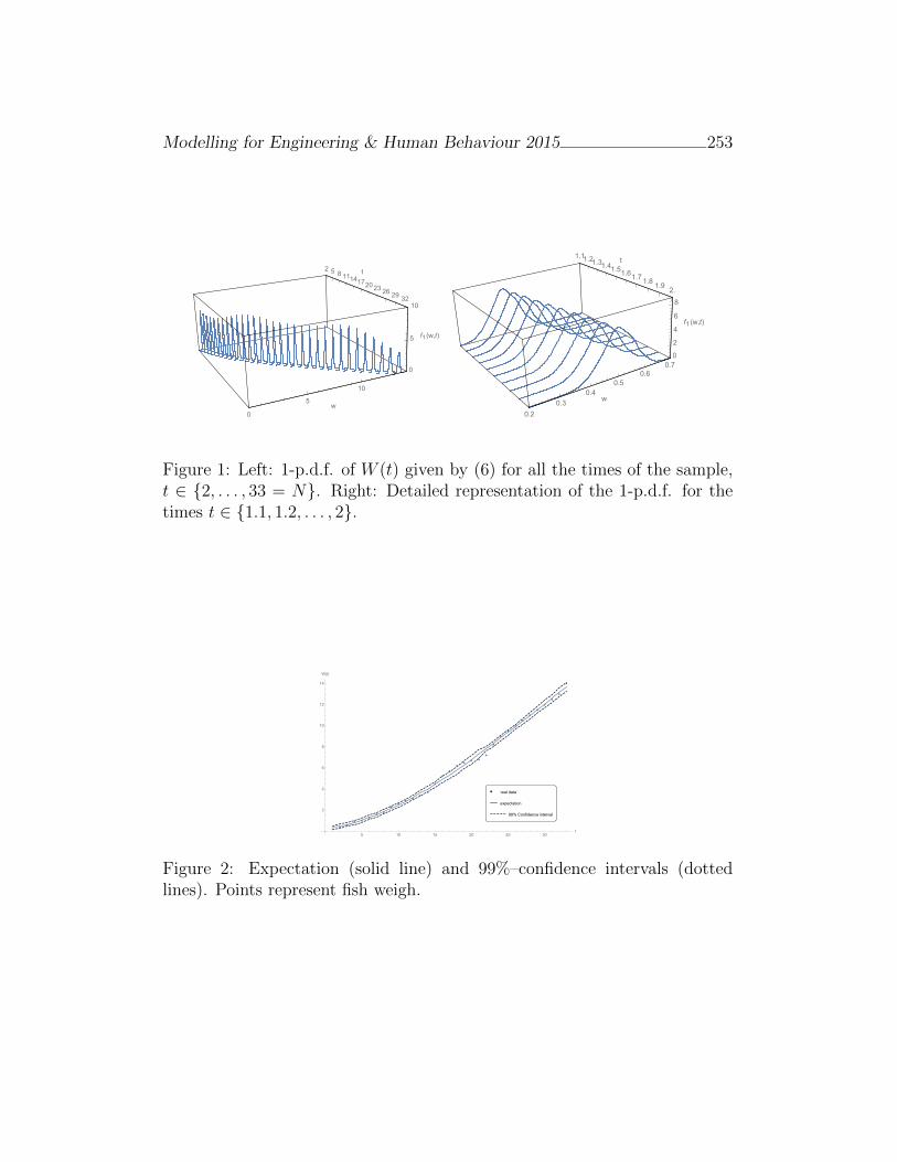
Modelling for Engineering & Human Behaviour 2015 253
2 5 8 1114172023 26 29 32
t
0
5
10
w
0
5
10
f1 (w,t)
1.11.21.31.41.51.61.71.8
1.92.
t
0.2
0.3
0.40.5
0.60.7
w
0
2
4
6
8
f1 (w,t)
Figure 1: Left: 1-p.d.f. of W (t) given by (6) for all the times of the sample,t ∈ 2, . . . , 33 = N. Right: Detailed representation of the 1-p.d.f. for thetimes t ∈ 1.1, 1.2, . . . , 2.
5 10 15 20 25 30t
2
4
6
8
10
12
14
W(t)
real data
expectation
99% Confidence interval
Figure 2: Expectation (solid line) and 99%–confidence intervals (dottedlines). Points represent fish weigh.
Modelling for Engineering & Human Behaviour 2015 254
References
[1] T.T. Soong, Random Differential Equations in Science and Engineering.New York, Academic Press, 1973.
[2] Bertalanffy, L. von. A quantitative theory of organic growth (Inquirieson Growth Laws II) Human Biology, Volume(10): 181–213, 1938.
[3] Bertalanffy, L. von. Quantitative laws in metabolism and growth TheQuarterly Review of Biology, Volume(32): 217–231, 1957.
[4] M. C. Casaban, J. C. Cortes, J. V. Romero, M. D. Rosell o. Determin-ing the first probability density function of linear random initial valueproblems by the Random Variable Transformation (RVT) technique:A comprehensive study Abstract and Applied Analysis, Volume(2014) :1–25, 2014.
[5] M. C. Casaban, J. C. Cortes, J. V. Romero, M. D. Rosello. Probabilis-tic solution of random SI-type epidemiological models using the randomvariable transformation technique Communications in Nonlinear Sci-ence and Numerical Simulation Volume(24): 1–3, 2015.
[6] M. C. Casaban, J. C. Cortes, A. Navarro-Quiles, J. V. Romero, M.D. Rosello, R. J. Villanueva. Probabilistic solution of the homogeneousRiccati differential equation: A case-study by using linearization andtransformation techniques Journal of Computational of Applied Mathe-matics Volume(291): 20–35, 2016.
[7] L. v. Qiming, J. W. Pitchford. Stochastic von Bertalanffy models withapplications to fish recruitment Journal of Theoretical Biology Vol-ume(244): 640–655, 2007.
A front-fixing numerical method for a freeboundary nonlinear diffusion logistic
population model
M. A. Piqueras† ∗, R. Company† , and L. Jodar†
(†) Instituto de Matematica Multidisciplinar, Universitat Politecnica de Valencia,
Camino de Vera s/n, 46022 Valencia, Spain.
November 30, 2015
1 Introduction
The spatial-temporal spreading of a new invasive species in a habitat hasinterest in ecology and is modeled by a moving boundary diffusion logisticpartial differential problem, where the moving boundary represents the un-known expanding front of the species. In this paper a front-fixing approachis applied in order to transform the original moving boundary problem into afixed boundary one. A finite difference method preserving qualitative prop-erties of the theoretical solution is proposed. Results are illustrated withnumerical experiments.
The diffusive logistic model of [2] for the density of population of theinvasive species U(t, x) depending on time t and spatial variable x states asfollows
∂U
∂t−D∂
2U
∂x2= U(a− bU), t > 0, 0 < x < H(t), (1)
together with the boundary conditions
∂U
∂x(t, 0) = 0, U(t,H(t)) = 0, t > 0, (2)
∗e-mail: [email protected]
255
Modelling for Engineering & Human Behaviour 2015 256
the Stefan condition
H ′(t) = −µ∂U∂x
(t,H(t)), t > 0, (3)
and the initial conditions
H(0) = H0, U(0, x) = U0(x), 0 ≤ x ≤ H0. (4)
The initial function U0(x) satisfies the following properties
U0(x) ∈ C2([0, H0]), U ′0(0) = U0(H0) = 0, U0(x) > 0, 0 ≤ x < H0. (5)
Here H(t) is the unknown moving boundary such that the populationis distributed in the interval [0, H(t)], D > 0 is the dispersal rate and thepositive parameters a and b are the intrinsic growth rate and the intraspecificcompetition, respectively.
2 Transformation and discretization of the con-
tinuous problem
Let us consider the Landau transformation, [1, 3],
z(t, x) =x
H(t), W (t, z) = U(t, x). (6)
Under substitution (6) problem (1)-(4) takes the form
G(t)∂W
∂t−G′(t)z
2
∂W
∂z−D∂
2W
∂z2= G(t)W (a− bW ), t > 0, 0 < z < 1, (7)
whereG(t) = H2(t), t ≥ 0. (8)
Boundary conditions (2) and Stefan condition (3) take the form
∂W
∂z(t, 0) = 0, W (t, 1) = 0, t > 0, (9)
and
G′(t) = −2µ∂W
∂z(t, 1), t > 0, (10)
Modelling for Engineering & Human Behaviour 2015 257
respectively, while the initial conditions (4) become
G(0) = H20 , W (0, z) = W0(z) = U0(zH0), 0 ≤ z ≤ 1. (11)
Conditions (5) for the initial function U0(x) are translated to W0(z) asfollows
W0(z) ∈ C2([0, 1]), W ′0(0) = W0(1) = 0, W0(z) > 0, 0 ≤ z < 1. (12)
Let us consider the step size discretization k = ∆t, h = ∆z = 1/M , andthe mesh points (tn, zj), with tn = kn, n ≥ 0, zj = jh, 0 ≤ j ≤ M andM positive integer. Let us consider the forward approximation of the timederivatives
wn+1j − wnj
k≈ ∂W
∂t(tn, zj),
gn+1 − gn
k≈ G′(tn), (13)
and the central approximation of the spatial derivatives
wnj+1 − wnj−12h
≈ ∂W
∂z(tn, zj),
wnj−1 − 2wnj + wnj+1
h2≈ ∂2W
∂z2(tn, zj). (14)
Then, we have the following explicit scheme
gn+1 = gn +kµ
h(4wnM−1 − wnM−2), n ≥ 0, (15)
wn+1j = anjw
nj−1 + bnjw
nj + cnjw
nj+1, n ≥ 0, 0 ≤ j ≤M − 1, (16)
where the coefficients are given by
anj =k
h2
(D
gn−zjµ(4wnM−1 − wnM−2)
4gn
),
bnj = 1 + k(a− bwnj )− k
h22D
gn,
cnj =k
h2
(D
gn+zjµ(4wnM−1 − wnM−2)
4gn
). (17)
Modelling for Engineering & Human Behaviour 2015 258
3 Consistency
Let us consider the problem (7)-(11), denoted in vector form as L(W,G) =(L1(W,G),L2(W,G),L3(W,G)) where equations (7),(9), (11) are written inthe form
L1(W,G) =∂W
∂t−G
′(t)
G(t)
z
2
∂W
∂z− D
G(t)
∂2W
∂z2−W (a−bW ) = 0, t > 0, 0 < z < 1,
(18)
L2(W,G) =∂W
∂z(t, 0) = 0, t > 0, (19)
L3(W,G) = G′(t) + 2µ∂W
∂z(t, 1) = 0, t > 0, (20)
and the finite difference scheme, written together as L(w, g)= (L1(w, g), L2(w, g), L3(w, g)) where
L1(w, g) =wn+1j − wnj
k− zj
2
wnj+1 − wnj−12h
(gn+1 − gn
gnk
)−Dgnwnj−1 − 2wnj + wnj+1
h2− wnj (a− bwnj ) = 0, n ≥ 0, 0 ≤ j ≤M − 1,
(21)
L2(w, g) =wn1 − wn−1
2h= 0, n ≥ 0, (22)
L3(w, g) =gn+1 − gn
k− µ
h(4wnM−1 − wnM−2) = 0, n ≥ 0. (23)
It holds that the scheme L(w, g) is consistent with the problem L(W,G) andthe local truncation error behaves
T nj (W,G) = O(k) +O(h2). (24)
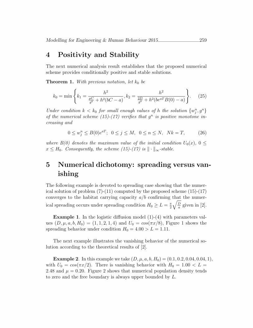
Modelling for Engineering & Human Behaviour 2015 259
4 Positivity and Stability
The next numerical analysis result establishes that the proposed numericalscheme provides conditionally positive and stable solutions.
Theorem 1. With previous notation, let k0 be
k0 = min
k1 =
h2
µCg0
+ h2(bC − a), k2 =
h2
2Dg0
+ h2(beaTB(0)− a)
. (25)
Under condition k < k0 for small enough values of h the solution wnj , gnof the numerical scheme (15)-(17) verifies that gn is positive monotone in-creasing and
0 ≤ wnj ≤ B(0)eaT ; 0 ≤ j ≤M, 0 ≤ n ≤ N, Nk = T, (26)
where B(0) denotes the maximum value of the initial condition U0(x), 0 ≤x ≤ H0. Consequently, the scheme (15)-(17) is ‖ · ‖∞-stable.
5 Numerical dichotomy: spreading versus van-
ishing
The following example is devoted to spreading case showing that the numer-ical solution of problem (7)-(11) computed by the proposed scheme (15)-(17)converges to the habitat carrying capacity a/b confirming that the numer-
ical spreading occurs under spreading condition H0 ≥ L = π2
√Da
given in [2].
Example 1. In the logistic diffusion model (1)-(4) with parameters val-ues (D,µ, a, b,H0) = (1, 1, 2, 1, 4) and U0 = cos(πx/8), Figure 1 shows thespreading behavior under condition H0 = 4.00 > L = 1.11.
The next example illustrates the vanishing behavior of the numerical so-lution according to the theoretical results of [2].
Example 2. In this example we take (D,µ, a, b,H0) = (0.1, 0.2, 0.04, 0.04, 1),with U0 = cos(πx/2). There is vanishing behavior with H0 = 1.00 < L =2.48 and µ = 0.20. Figure 2 shows that numerical population density tendsto zero and the free boundary is always upper bounded by L.
Modelling for Engineering & Human Behaviour 2015 260
0 5 10 15 20 25 300
0.5
1
1.5
2
2.5
3
3.5
x
U (
t, x)
t = 4t = 3t = 2t = 1t = 0Habitat carrying capacity a/b = 2.00
Fig. 1. Numerical solution for several values of time in a spreading case.
0 0.5 1 1.5 2 2.50
0.2
0.4
0.6
0.8
1
x
U (
t, x)
t = 10t = 8t = 6t = 4t = 2t = 0
Spreading barrier L = 2.48
Fig. 2. Numerical solution for several values of time in a vanishing case.
References
[1] J. Crank, Free and Moving Boundary Problems, Oxford Science Publi-cations, 1984.
[2] Y. Du, Z. Lin, Spreading-vanishing dichotomy in the diffusive logisticmodel with a free boundary, SIAM J. Math. Anal., 42(1):377–405, 2010.
[3] H. G. Landau, Heat condution in a melting solid, Quarterly of AppliedMathematics, 8:81–95, 1950.
A computational study on the influence ofconvergent-divergent orifices on the inner flowand cavitation development in diesel injector
nozzles
F.J. Salvador[∗, D. Jaramillo-Cıscar[, J.-V. Romero† andM.-D. Rosello†
([) CMT-Motores Termicos, Universitat Politecnica de Valencia,
Camino de Vera s/n, Edificio 6D, 46022 Valencia, Spain,
(†) Instituto de Matematica Multidisciplinar, Universitat Politecnica de Valencia,
Camino de Vera s/n, Edificio 8G, 2, 46022 Valencia, Spain
November 30, 2015
1 Introduction
Nowadays modern diesel engines are facing to the improvement in the fuelconsumption and the reduction of pollutant emissions. The first step beforeto study the combustion process or the air-fuel mixing process is to studythe flow behaviour inside the diesel injector that will be the responsible forthe subsequent processes.
In order to accomplish with the required improvement, non-conventionalorifices have been studied in the recent years [1–5]. Those studies involvethe use of elliptical nozzles [1–3] and divergent nozzles [4,5]. The aim of thisstudy is to increase the available information on non-conventional orifices indiesel injectors. For that reason 3 convergent-divergent nozzles have been
∗Corresponding author, Dr. F. Javier Salvador, e-mail: [email protected], Tele-phone: 34-963879659, Fax: 34-963877659
261

Modelling for Engineering & Human Behaviour 2015 262
numerically studied. Due to the divergent component of the orifices, thecavitation phenomenon plays an important role in the flow behaviour. Thiskind of geometry is common in other areas as acoustic [6] and refrigerationsystems [7].
The present extended abstract has been divided into 5 sections. First ofall, a brief description of the computational fluid dynamics (CFD) approachused to study the cavitation phenomenon is performed in section 2. Thegeometry characteristics for the three convergent-divergent nozzles that havebeen studied are explained in section 3. The results of the study are presentedin section 4 and finally, the main conclusions are drawn in section 5.
2 Description of the CFD approach
The study has been performed with a code previously validated [8,9] and ableto simulate cavitation phenomenon using a homogeneous equilibrium model(HEM). The HEM is based in the assumption that the liquid and vapourphases are in each cell completely mixed and in equilibrium. The model usea barotropic equation of state to relate the density and the pressure. Thecompressibility on each cell depends on the liquid and the vapour phases.
The turbulence is modelled using a RANS approach. This method solvesthe Reynolds-averaged Navier Stokes (RANS) equations which models tur-bulent quantities, decomposing the fluid properties into an averaged and afluctuating component. From previous studies the RNG k-ε model has beenshown to be the best option to model the turbulence.
3 Geometry and boundary conditions
A multi-hole nozzle with 7 orifices has been used as a basis. Due to thesymmetry of the geometry the full nozzle is reduced to only 1 of the 7 orifices(51.4o). The orifices of the 3 convergent-divergent nozzles that have beenstudied are composed as shown in the Figure 1 of an initial convergent partuntil the middle of the orifice and a divergent part from the middle until theoutlet. The convergent and the divergent part are selected to be symmetrical,so the inlet and the outlet diameters, denoted by Di and D0 respectively, arethe same. The geometrical characteristics regarding the orifices can be foundat Table 1, whereDmid is the middle diameter and k-factor the conicity factor.

Modelling for Engineering & Human Behaviour 2015 263
Figure 1: Orifice’s geometry.
Nozzle θ [o] Dmid [µm] D0 [µm] k-factorcon [–]CD-2.5 2.5 124.6 156.3 3.2CD-3.5 3.5 124.6 169.0 4.4CD-4.5 4.5 124.6 181.7 5.7
Table 1: Geometrical characteristics of the orifices
For each part of the orifice the k-factor is defined as follows:
k-factorcon =Di −Dmid
10µm(1)
k-factordiv =Dmid −D0
10µm(2)
As the inlet and the outlet diameters are the same both k-factors havethe same absolute value but different sign. For that reason any reference tothe k-factor will be in absolute value.
k-factordiv = −k-factorcon (3)
For the simulations a fixed pressure condition has been used at the entrywhile for the outlet a mean pressure condition has been used. The mean
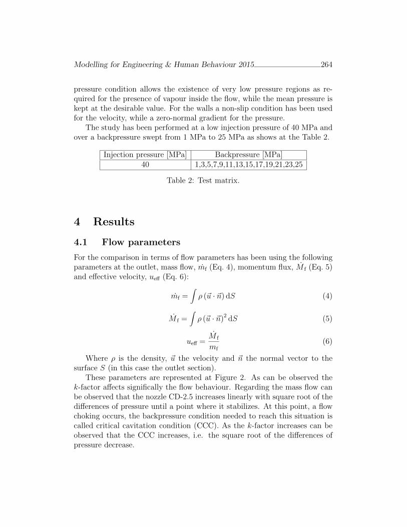
Modelling for Engineering & Human Behaviour 2015 264
pressure condition allows the existence of very low pressure regions as re-quired for the presence of vapour inside the flow, while the mean pressure iskept at the desirable value. For the walls a non-slip condition has been usedfor the velocity, while a zero-normal gradient for the pressure.
The study has been performed at a low injection pressure of 40 MPa andover a backpressure swept from 1 MPa to 25 MPa as shows at the Table 2.
Injection pressure [MPa] Backpressure [MPa]40 1,3,5,7,9,11,13,15,17,19,21,23,25
Table 2: Test matrix.
4 Results
4.1 Flow parameters
For the comparison in terms of flow parameters has been using the followingparameters at the outlet, mass flow, mf (Eq. 4), momentum flux, M f (Eq. 5)and effective velocity, ueff (Eq. 6):
mf =∫ρ (~u · ~n) dS (4)
M f =∫ρ (~u · ~n)2 dS (5)
ueff =M f
mf
(6)
Where ρ is the density, ~u the velocity and ~n the normal vector to thesurface S (in this case the outlet section).
These parameters are represented at Figure 2. As can be observed thek-factor affects significally the flow behaviour. Regarding the mass flow canbe observed that the nozzle CD-2.5 increases linearly with square root of thedifferences of pressure until a point where it stabilizes. At this point, a flowchoking occurs, the backpressure condition needed to reach this situation iscalled critical cavitation condition (CCC). As the k-factor increases can beobserved that the CCC increases, i.e. the square root of the differences ofpressure decrease.
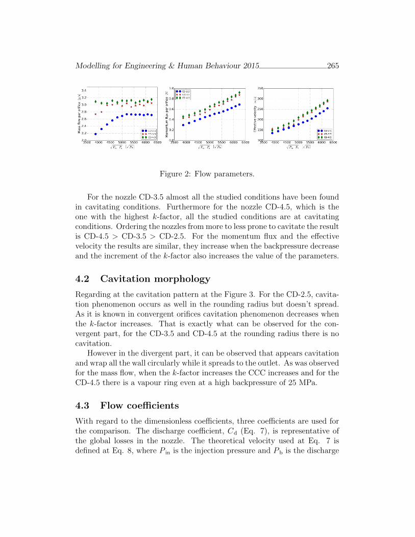
Modelling for Engineering & Human Behaviour 2015 265
Figure 2: Flow parameters.
For the nozzle CD-3.5 almost all the studied conditions have been foundin cavitating conditions. Furthermore for the nozzle CD-4.5, which is theone with the highest k-factor, all the studied conditions are at cavitatingconditions. Ordering the nozzles from more to less prone to cavitate the resultis CD-4.5 > CD-3.5 > CD-2.5. For the momentum flux and the effectivevelocity the results are similar, they increase when the backpressure decreaseand the increment of the k-factor also increases the value of the parameters.
4.2 Cavitation morphology
Regarding at the cavitation pattern at the Figure 3. For the CD-2.5, cavita-tion phenomenon occurs as well in the rounding radius but doesn’t spread.As it is known in convergent orifices cavitation phenomenon decreases whenthe k-factor increases. That is exactly what can be observed for the con-vergent part, for the CD-3.5 and CD-4.5 at the rounding radius there is nocavitation.
However in the divergent part, it can be observed that appears cavitationand wrap all the wall circularly while it spreads to the outlet. As was observedfor the mass flow, when the k-factor increases the CCC increases and for theCD-4.5 there is a vapour ring even at a high backpressure of 25 MPa.
4.3 Flow coefficients
With regard to the dimensionless coefficients, three coefficients are used forthe comparison. The discharge coefficient, Cd (Eq. 7), is representative ofthe global losses in the nozzle. The theoretical velocity used at Eq. 7 isdefined at Eq. 8, where P in is the injection pressure and P b is the discharge

Modelling for Engineering & Human Behaviour 2015 266
Figure 3: Cavitation pattern.
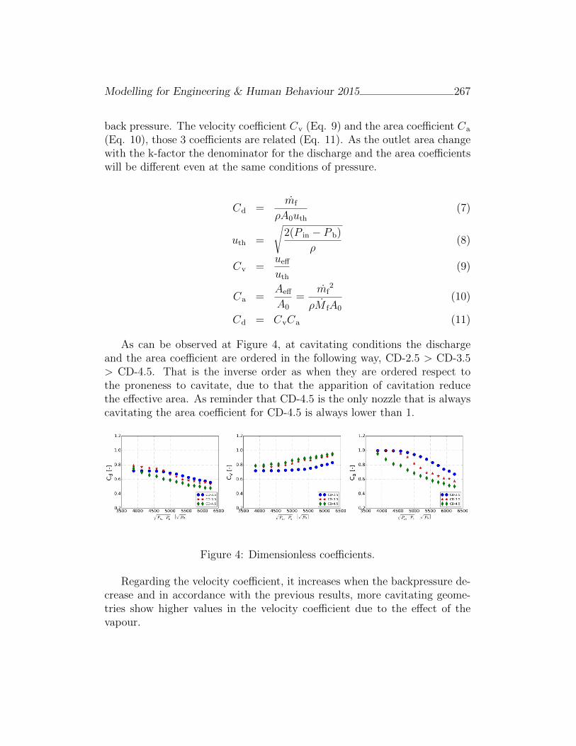
Modelling for Engineering & Human Behaviour 2015 267
back pressure. The velocity coefficient Cv (Eq. 9) and the area coefficient Ca
(Eq. 10), those 3 coefficients are related (Eq. 11). As the outlet area changewith the k-factor the denominator for the discharge and the area coefficientswill be different even at the same conditions of pressure.
Cd =mf
ρA0uth
(7)
uth =
√2(P in − P b)
ρ(8)
Cv =ueff
uth
(9)
Ca =Aeff
A0
=mf
2
ρM fA0
(10)
Cd = CvCa (11)
As can be observed at Figure 4, at cavitating conditions the dischargeand the area coefficient are ordered in the following way, CD-2.5 > CD-3.5> CD-4.5. That is the inverse order as when they are ordered respect tothe proneness to cavitate, due to that the apparition of cavitation reducethe effective area. As reminder that CD-4.5 is the only nozzle that is alwayscavitating the area coefficient for CD-4.5 is always lower than 1.
Figure 4: Dimensionless coefficients.
Regarding the velocity coefficient, it increases when the backpressure de-crease and in accordance with the previous results, more cavitating geome-tries show higher values in the velocity coefficient due to the effect of thevapour.
Modelling for Engineering & Human Behaviour 2015 268
5 Conclusions
The main conclusions of this study are summarized in the following points:
• Due to the divergent part of the orifice, the Convergent-Divergent noz-zles are more prone to cavitate (even at high backpressure conditions).The k-factor influences the appearance of cavitation (CD-4.5 > CD-3.5> CD-2.5).
• The effective velocity is increased with the k-factor in this types ofnozzles. Together with the increase of cavitation, a better quality inthe air-fuel mixing process is presupposed for higher k-factor.
• As it is known, high k-factor in convergent nozzles prevents cavitationto appear in the rounding radius. And that has been obtained. ForCD-2.5, a small amount of vapour appears at the rounding radius asidethe divergent part, while for CD-3.5 and CD-4.5 cavitation just appearsin the divergent part but not in the rounding radius.
Acknowledgments
The authors would like to express gratitude for the computer resources, tech-nical expertise and assistance provided by the Universidad de Valencia relat-ing to the use of the supercomputer “Tirant”.
References
[1] Chih Ming Ho and Ephraim Gutmark. Vortex induction and mass en-trainment in a small-aspect-ratio elliptic jet. Journal of Fluid Mechanics,179:383–405, 1987.
[2] Fazle Hussain and Hyder S. Husain. Elliptic jets. Part 1. Characteristicsof unexcited and excited jets. Journal of Fluid Mechanics, 208:257–320,1989.
[3] S. Molina, F.J. Salvador, M. Carreres, and D. Jaramillo. A computationalinvestigation on the influence of the use of elliptical orifices on the innernozzle flow and cavitation development in diesel injector nozzles. EnergyConversion and Management, 79:114–127, mar 2014.

Modelling for Engineering & Human Behaviour 2015 269
[4] J. Benajes, S. Molina, C. Gonzalez, and R. Donde. The role of nozzleconvergence in diesel combustion. Fuel, 87(10-11):1849–1858, aug 2008.
[5] Ozgur Oguz Taskiran and Metin Ergeneman. Effect of nozzle dimensionsand fuel type on flame lift-off length. Fuel, 115:833–840, jan 2014.
[6] Chih-Chung Hu, Win-Ti Lin, Chun-Min Su, and Wen-Jay Liu. Dischargecharacteristics of small sonic nozzles in the shape of pyramidal convergentand conical divergent. Flow Measurement and Instrumentation, 25:26–31,jun 2012.
[7] Jinghui Liu, Jiangping Chen, and Zhijiu Chen. Critical flashing flow inconvergentdivergent nozzles with initially subcooled liquid. InternationalJournal of Thermal Sciences, 47(8):1069–1076, aug 2008.
[8] F.J. Salvador, J.-V. Romero, M.-D. Rosello, and J. Martınez-Lopez. Val-idation of a code for modeling cavitation phenomena in Diesel injectornozzles. Mathematical and Computer Modelling, 52(7-8):1123–1132, oct2010.
[9] F. Payri, R. Payri, F.J. Salvador, and J. Martınez-Lopez. A contribu-tion to the understanding of cavitation effects in Diesel injector nozzlesthrough a combined experimental and computational investigation. Com-puters & Fluids, 58:88–101, apr 2012.
Mixed Truck Delivery Systems with bothHub-and-Spoke and Direct Shipment
B. Royo[ ∗, D. Escuin†, A. Fraile[, JA. Sicilia‡, and E. Larrode[
([) Universidad de Zaragoza,
Calle Marıa de Luna 3, 50018, Zaragoza,
(†) Instituto Tecnologico de Aragon,
Calle Marıa de Luna 7, 50018, Zaragoza,
(‡) Universidad Internacional de La Rioja (UNIR),
Gran Vıa Rey Juan Carlos I, 41. 26002 Logrono, La Rioja.
November 30, 2015
1 Introduction
Progress of the supply chain management and the increase of e-commerceplaces the freight motor carriers to consider strategies and tactics to min-imize costs while maintaining a high service quality. Therefore, [1] definesdifferent distribution strategies networks: many to many, hub&spoke andpeddling&collecting, which are usually studied separately.Several studies show positive effects of mixing strategies. The following pa-pers: [2], [3], [4], [5], [6], [7], etc., developed metaheuristics to solve differentcombined scenarios.In this case, a linear programming model of a mixed delivery system solvedin [6], is proposed. Previous researches have developed mathematical formu-lation as in [8], [9] and [10], however, to the best of our knowledge this is thefirst study to model a mixed delivery system with several hubs, stopoversand time constraints.
∗e-mail:[email protected]
270
Modelling for Engineering & Human Behaviour 2015 271
2 Problem description
This paper deals with the load planning problem of lessthantruckload motorcarriers, the determination of how freight should be routed through the net-work to minimize costs while maintaining service.The main features of the problem are: an order consists on a pickup anda delivery node with small freight and time windows; to be managed it isallowed to go through at least one “hub”, to stop among direct shipments,to stop between “hub” node or node“hub” connections and the “hubs” arelinked but stopovers are not allowed.
3 Mathematical Formulation
The following lists the assumption, the required parameters and the decisionvariables to formulate the problem.
Assumptions:Each order o ∈ O consists on a pickup i ∈ N and a delivery node j ∈ N withcij as the shortest distance among them. The service time in a node is takenas ti.
Input Data:Ho, Hd the set of origin and destination “hubs” respectively and R and Eare the set of pickup and delivery nodes where N = Ho ∪Hd ∪R ∪ E.Let di ∈ N the delivery node of the pickup node i ∈ N and ah ∈ N the“hubs” pickup node of the delivery node h ∈ N .V consists on the set of vehicles with a capacity Q and they are not allowedto arrived before ei and after li and mi as the amount of freight in node i ∈ N .
Zero one decision variables:
xvij =
1 If v ∈ V goes form node i ∈ Nto node j ∈ N.
0 otherwise.(1)
yih =
1 If i ∈ R ∪ E starts or ends in “hubs” h ∈ Ho.
0 otherwise.(2)
Modelling for Engineering & Human Behaviour 2015 272
uij =
1 If a line trip goes from “hubs”i, to “hubs”j ∈ Ho.
0 otherwise.(3)
Other variables are svi , i ∈ N, v ∈ V is the arrival time at node i by thevehicle v and qvi , i ∈ N, v ∈ V is the amount of available capacity of thevehicle v in the node i.
Objective functionThe minimization of the total distance including the distance among “hubs”:
min∑k∈V
∑i∈N
∑j∈N
cijxkij +
∑i∈Ho
∑j∈Ho
cijuij (4)
Subject to constraints: ∑h∈Ho
∑i∈Hd∪E
xvhi = 1 ∀v ∈ V (5)
∑i∈Ho∪R
∑h∈Hd
xvih = 1 ∀v ∈ V (6)
xvdp = 0 ∀v ∈ V, ∀p ∈ R, ∀d ∈ E (7)
∑v∈V
∑j∈N
xvij = 1 ∀i ∈ N (8)
xvii = 0 ∀v ∈ V, ∀i ∈ N (9)
∑i∈Ho∪R∪E,i!=j
xvij −
∑i∈Hd∪R∪E,i!=j
xvji = 0 ∀v ∈ V, ∀j ∈ R ∪ E (10)
5, 6 ensure no pickup node after arriving at Ho and no delivery nodebefore leaving Ho, 7 to prevent any pickup node precedes any delivery node,8,9 guarantee every node is visited only once and 10 is the flow conservationequation that ensures the continuity of each vehicle route.
Modelling for Engineering & Human Behaviour 2015 273
1− xvdo2do1
−∑h∈Hd
∑o∈R
xvoh ≤ (1− xv
o1o2)M ∀v ∈ V, ∀o1, o2 ∈ R (11)
1−∑o1∈R
∑h2∈Hd
xvo1h2− xv
h2do1≤ (1− xv
oh)M ∀v ∈ V, ∀o ∈ R, ∀h ∈ Ho (12)
xvoe = 0 ∀v ∈ V, ∀o ∈ R, ∀e ∈ E, do! = e (13)
11, 12 y 13 ensure all pickup nodes precede delivery nodes following last-in-first-out policy in direct shipments.
1− ydoh ≤ (2−∑
j∈R∪Ho
xvjh −
∑j∈Ho∪R
xvoj)M ∀v ∈ V, ∀o ∈ R, ∀h ∈ Hd ∪Ho
(14)
1− ydh ≤ (2−∑
j∈E∪Hd
xvhj −
∑j∈E
xvdj)M ∀v ∈ V, ∀d ∈ E,∀h ∈ Ho (15)
1− uh1h2 ≤ (2− yoh1 − ydoh2)M ∀o ∈ R, ∀h1 ∈ Ho, h2 ∈ Hd (16)
14 and 15 identify pickup or delivery routes from a node to a Ho and from aHd to a node respectively. 16 refers routes among “hubs”.
svh = 0 ∀v ∈ V, ∀h ∈ Hd (17)
svi + ti − svj + cij ≤ (1− xvij)M ∀v ∈ V, ∀i, j ∈ N (18)
ei ≤ svi ∀v ∈ V, ∀i ∈ N (19)
Modelling for Engineering & Human Behaviour 2015 274
svi ≤ li ∀v ∈ V, ∀i ∈ N (20)
17and 18 show how to obtain values related to time. 19 y 20 refers timewindows boundaries.
qvi ≤ Q ∀v ∈ V, ∀i ∈ N (21)
qvh ≤ (1− xvhj)M ∀v ∈ V, ∀j ∈ R, ∀h ∈ Ho (22)
qvi + mj − qvj ≤ (1− xvij)M ∀v ∈ V, ∀i ∈ Ho ∪R, ∀j ∈ R ∪Hd (23)
qvi ≤ (1− xvij)M ∀v ∈ V, ∀i ∈ E,∀j ∈ Hd (24)
qvj + mj − qvi ≤ (1− xvij)M ∀v ∈ V, ∀i ∈ E ∪Ho (25)
qvi + mj − qvj ≤ (1− xvij)M ∀v ∈ V, ∀i ∈ R, ∀j ∈ E (26)
Vehicles cannot exceed capacity as is ensured in 21,22,23,24,25 and 26.
4 Conclusions
To the best of our knowledge, our is the first study to develop a mathematicalmodel representing a transport scenery where features of different problemsconverge as ’less than truckload, hub allocation, long distances, time win-dows, route planing, direct shipments allowing stopovers and hub shipmentsallowing stopovers’.This research could be extended by considering more constraints as limits onthe hubs’ capacity or on hubs’ operational time.
References
[1] Estrada, M. Efficient distribution strategies for less-than-truckload car-riers. PhD. thesis. School of Civil Engineering, Technical University ofCatalonia, Spain., 2007
Modelling for Engineering & Human Behaviour 2015 275
[2] Jiyin Liu, Chung-Lun Li and Chun-Yan Chan. Mixed truck deliverysystems with both hub-and-spoke and direct shipment TransportationResearch Part E: Logistics and Transportation Review, Volume(39):325-339, 2003
[3] Kuby, M. J. and Gray, R. G. The hub network design problem withstopovers and feeders: The case of federal express. Transportation Re-search Part A: Policy and Practice, Volume(27):1-12, 1993
[4] Kuo, Y. and Wang, C.-C. A variable neighborhood search for the mul-tidepot vehicle routing problem with loading cost. Expert Systems withApplications, Volume(39):6949-6954, 2012.
[5] Crevier, B., Cordeau, J.-F. and Laporte, G. The multi-depot vehiclerouting problem with inter-depot routes. European Journal of Opera-tional Research, Volume(176):756-773, 2007.
[6] Royo, B. Fraile, A. Larrode, E. and Muerza, V. Route planning fora mixed delivery system in long distance transportation and compari-son with pure delivery systems. Journal of Computational and AppliedMathematics, Volume(291):488-496, 2015.
[7] Caramia, M. and Guerriero, F. A heuristic approach to long-haul freight transportation with multiple objective functions. Omega,Volume(37):600-614, 2009.
[8] Aykin, T. The hub location and routing problem. European Journal ofOperational Research, Volume(83):200-219, 1995.
[9] Cheng-Chang Lin and Sheu-Hua Chen. An integral constrained gen-eralized hub-and-spoke network design problem. Transportation Re-search Part E: Logistics and Transportation Review, Volume(44):986-1003, 2008.
[10] Hande Yaman, Bahar Y. Kara and Barbaros C. Tansel. The latest ar-rival hub location problem for cargo delivery systems with stopovers.Transportation Research Part B: Methodological, Volume(41):906-919,2007.
A proposal to classify the epidemiologicalbehavior of a network model of meningococcal
C using ROC method
L. Acedo[ ∗, R.-M. Shoucri†, R.-J. Villanueva‡
([) Instituto Universitario de Matematica Multidiciplinar,
Universitat Politecnica de Valencia, Valencia, Spain,
(†) Department of Mathematics & Computer Science,
Royal Military College of Canada,
(‡) Instituto Universitario de Matematica Multidiciplinar,
Universitat Politecnica de Valencia, Valencia, Spain.
November 30, 2015
1 Introduction
Meningococcal disease is caused by the bacterium Neisseria meningitidis, alsocalled meningococcus. About 10% of people have this type of bacteria in theback of their nose and throat with no signs or symptoms of disease, beingcalled carrier. But sometimes Neisseria meningitidis bacteria can invade thebody causing certain illnesses, which are known as meningococcal diseases[1].
Neisseria meningitidis bacteria are spread through the exchange of respi-ratory and throat secretions like spit (e.g., living in close quarters, kissing,sharing drinks). Fortunately, these bacteria are not as contagious as whatcauses the common cold or the flu. Besides, the bacteria are not spread by
∗e-mail: [email protected]
276
Modelling for Engineering & Human Behaviour 2015 277
casual contact or by simply breathing the air where a person with meningo-coccal disease has been. Sometimes Neisseria meningitidis bacteria spread topeople who have had close or lengthy contact with a patient with meningo-coccal disease. People in the same household, roommates, or anyone withdirect contact with a patient’s oral secretions, meaning saliva or spit, (suchas a boyfriend or girlfriend) would be considered at increased risk of gettingthe infection [1]
Meningitis is an infection of the brain and spinal cord and can even infectthe blood. Nowadays the main cause of Meningitis is the bacterium Neisse-ria meningitidis. This bacterium is transmitted exclusively among humans,mainly during adolescence. An individual may get infected by contact with acarrier individual, that is, healthy carriers transmit the bacteria. It is treatedwith specific antibiotic, however, even properly treated, there is up to 10%of mortality and 10% of survivors have sequelae [2, 3].
Recently, network models under a computational (simulations) point ofview are being used to study the short-medium term transmission dynamicsof infectious diseases and to find sets of feasible model parameters by fittingmodel with data. Also, the network modeling allows to include randomnessin a natural way in the model simulations [4, 5].
One of the main problems in the study of the transmission dynamics ofMen C is that there is a lack of reliable data, because the time of carrieris very short (around 3 months), much less than the duration of a typicalclinical trial. Moreover, there are facts well know, as Men C may have cyclicalbehavior: every 7 (more or less) years there is an outbreak of Men C in Africa.
However in a network under a computational point of view, we need toolsthat allow us to classify the behavior of the model outputs. With these tools:
• we could determine the area of the parameters space responsible of adetermined behavior,
• the knowledge of these parameters could help us to understand betterits transmission dynamics,
• the knowledge of these parameters could help us to determine if thecyclic behavior is also characteristic of other places (for instance, Eu-rope).
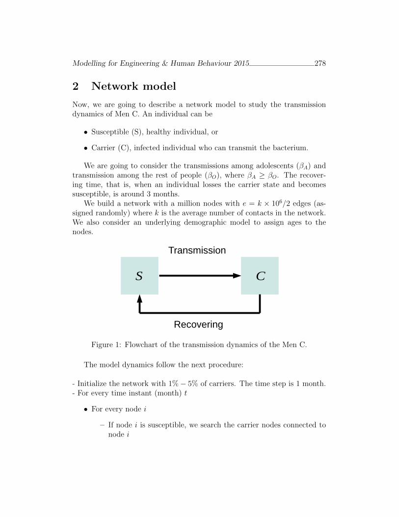
Modelling for Engineering & Human Behaviour 2015 278
2 Network model
Now, we are going to describe a network model to study the transmissiondynamics of Men C. An individual can be
• Susceptible (S), healthy individual, or
• Carrier (C), infected individual who can transmit the bacterium.
We are going to consider the transmissions among adolescents (βA) andtransmission among the rest of people (βO), where βA ≥ βO. The recover-ing time, that is, when an individual losses the carrier state and becomessusceptible, is around 3 months.
We build a network with a million nodes with e = k × 106/2 edges (as-signed randomly) where k is the average number of contacts in the network.We also consider an underlying demographic model to assign ages to thenodes.
S C
Transmission
Recovering
Figure 1: Flowchart of the transmission dynamics of the Men C.
The model dynamics follow the next procedure:
- Initialize the network with 1%− 5% of carriers. The time step is 1 month.- For every time instant (month) t
• For every node i
– If node i is susceptible, we search the carrier nodes connected tonode i
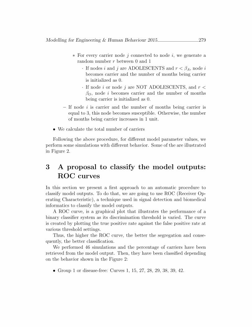
Modelling for Engineering & Human Behaviour 2015 279
∗ For every carrier node j connected to node i, we generate arandom number r between 0 and 1
· If nodes i and j are ADOLESCENTS and r < βA, node ibecomes carrier and the number of months being carrieris initialized as 0.
· If node i or node j are NOT ADOLESCENTS, and r <βO, node i becomes carrier and the number of monthsbeing carrier is initialized as 0.
– If node i is carrier and the number of months being carrier isequal to 3, this node becomes susceptible. Otherwise, the numberof months being carrier increases in 1 unit.
• We calculate the total number of carriers
Following the above procedure, for different model parameter values, weperform some simulations with different behavior. Some of the are illustratedin Figure 2.
3 A proposal to classify the model outputs:
ROC curves
In this section we present a first approach to an automatic procedure toclassify model outputs. To do that, we are going to use ROC (Receiver Op-erating Characteristic), a technique used in signal detection and biomedicalinformatics to classify the model outputs.
A ROC curve, is a graphical plot that illustrates the performance of abinary classifier system as its discrimination threshold is varied. The curveis created by plotting the true positive rate against the false positive rate atvarious threshold settings.
Thus, the higher the ROC curve, the better the segregation and conse-quently, the better classification.
We performed 46 simulations and the percentage of carriers have beenretrieved from the model output. Then, they have been classified dependingon the behavior shown in the Figure 2:
• Group 1 or disease-free: Curves 1, 15, 27, 28, 29, 38, 39, 42.
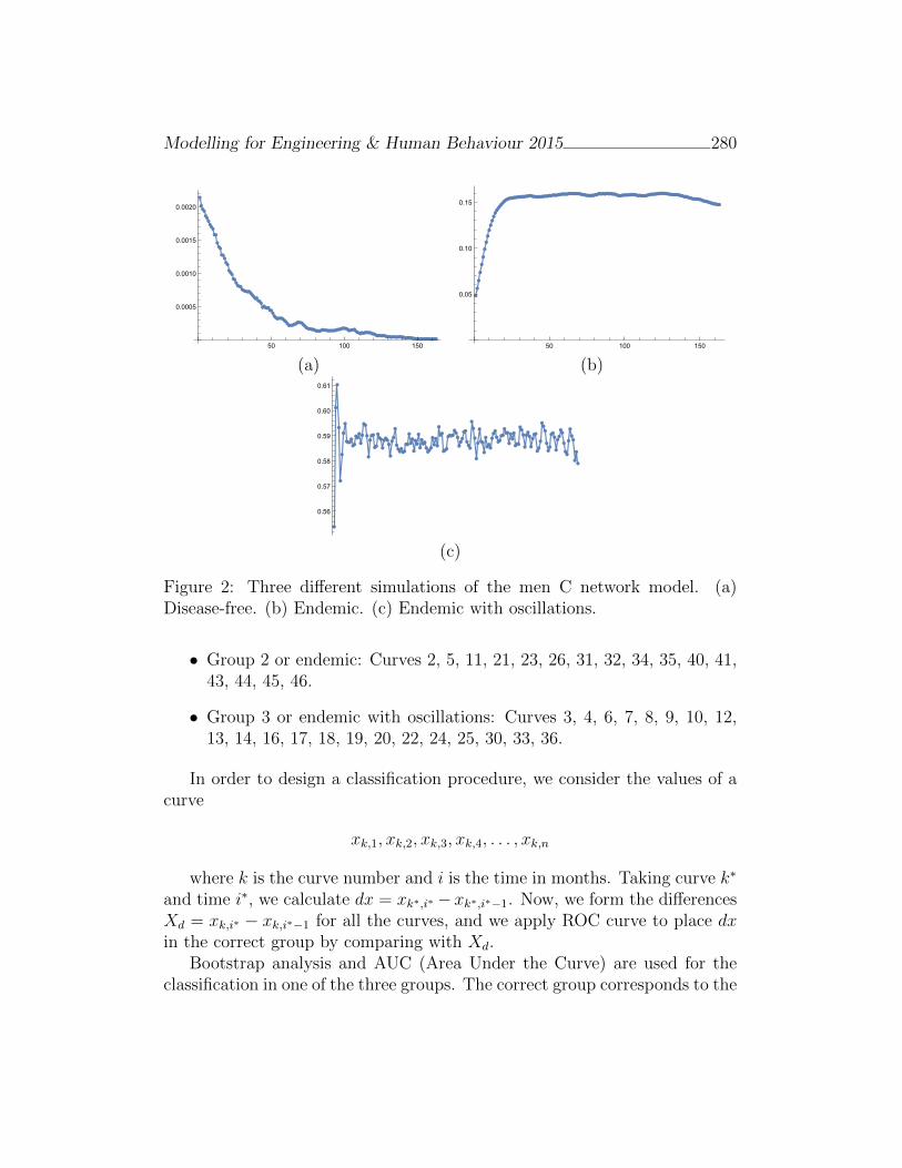
Modelling for Engineering & Human Behaviour 2015 280
50 100 150
0.0005
0.0010
0.0015
0.0020
50 100 150
0.05
0.10
0.15
(a) (b)
0.56
0.57
0.58
0.59
0.60
0.61
(c)
Figure 2: Three different simulations of the men C network model. (a)Disease-free. (b) Endemic. (c) Endemic with oscillations.
• Group 2 or endemic: Curves 2, 5, 11, 21, 23, 26, 31, 32, 34, 35, 40, 41,43, 44, 45, 46.
• Group 3 or endemic with oscillations: Curves 3, 4, 6, 7, 8, 9, 10, 12,13, 14, 16, 17, 18, 19, 20, 22, 24, 25, 30, 33, 36.
In order to design a classification procedure, we consider the values of acurve
xk,1, xk,2, xk,3, xk,4, . . . , xk,n
where k is the curve number and i is the time in months. Taking curve k∗
and time i∗, we calculate dx = xk∗,i∗ −xk∗,i∗−1. Now, we form the differencesXd = xk,i∗ − xk,i∗−1 for all the curves, and we apply ROC curve to place dxin the correct group by comparing with Xd.
Bootstrap analysis and AUC (Area Under the Curve) are used for theclassification in one of the three groups. The correct group corresponds to the
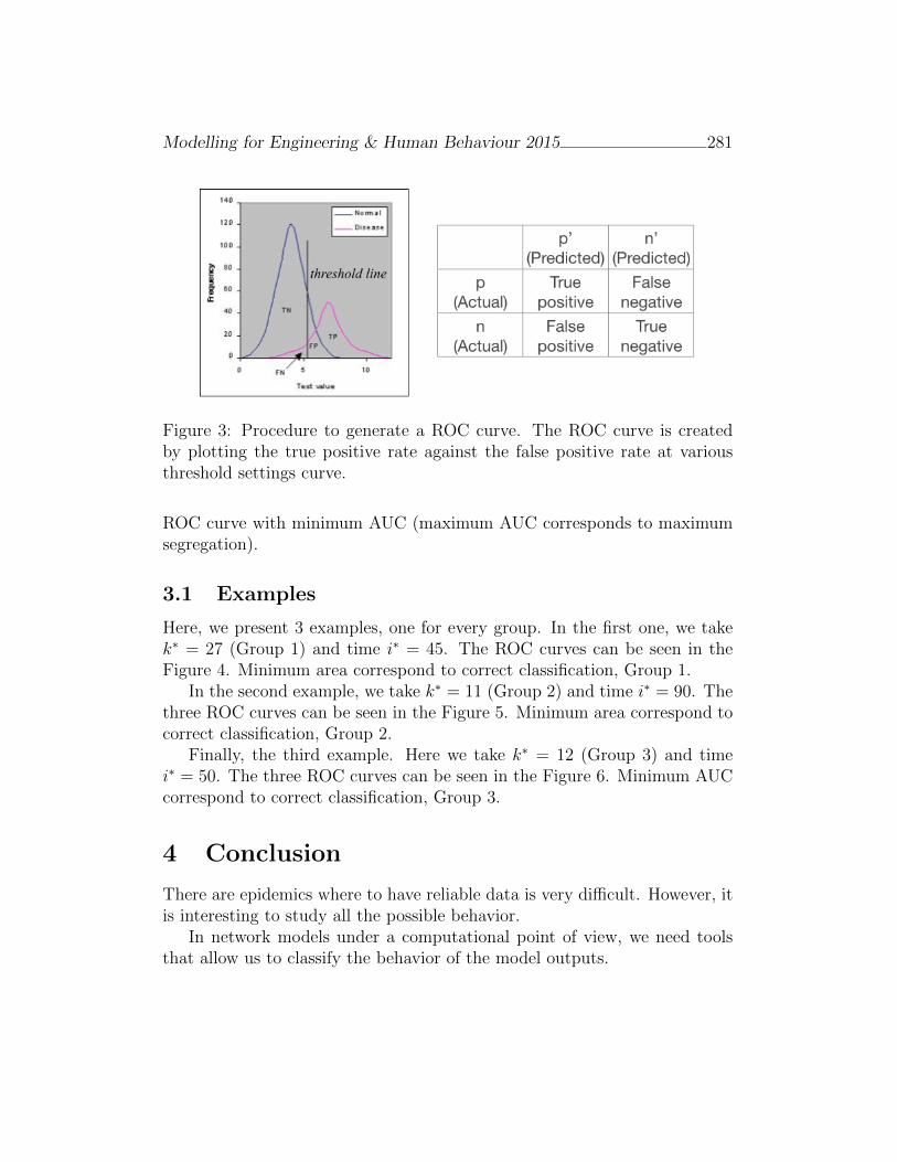
Modelling for Engineering & Human Behaviour 2015 281
Figure 3: Procedure to generate a ROC curve. The ROC curve is createdby plotting the true positive rate against the false positive rate at variousthreshold settings curve.
ROC curve with minimum AUC (maximum AUC corresponds to maximumsegregation).
3.1 Examples
Here, we present 3 examples, one for every group. In the first one, we takek∗ = 27 (Group 1) and time i∗ = 45. The ROC curves can be seen in theFigure 4. Minimum area correspond to correct classification, Group 1.
In the second example, we take k∗ = 11 (Group 2) and time i∗ = 90. Thethree ROC curves can be seen in the Figure 5. Minimum area correspond tocorrect classification, Group 2.
Finally, the third example. Here we take k∗ = 12 (Group 3) and timei∗ = 50. The three ROC curves can be seen in the Figure 6. Minimum AUCcorrespond to correct classification, Group 3.
4 Conclusion
There are epidemics where to have reliable data is very difficult. However, itis interesting to study all the possible behavior.
In network models under a computational point of view, we need toolsthat allow us to classify the behavior of the model outputs.
Modelling for Engineering & Human Behaviour 2015 282
Here we have presented a first approach with the goal of classifying thebehavior of the output of a network model of Men C. We have selected adifference on one curve, and then tried to classify it in one of the threegroups; generally it works, we get the correct group; but there is still workto be done to improve the classification algorithm, study accuracy, etc.
References
[1] http://www.cdc.gov/meningococcal/index.html
[2] Cartwright K.,Meningococcal carriage and disease. In: Cartwright K.,editor. Meningococcal disease. Chichester, UK: John Wiley & Sons; p.71-114, 1995.
[3] De Walls P. Immunization strategies for the control of serogroup Cmeningococcal disease in developed countries. Expert Rev Vaccines 5:269-75, 2006.
[4] L. Acedo, J.-A. Morano, R.-J. Villanueva, J. Villanueva-Oller, J. Diez-Domingo, Using random networks to study the dynamics of respiratorysyncytial virus (RSV) in the Spanish region of Valencia, Mathematicaland Computer Modelling, Volume 54 (7?8): 1650-1654, 2011.
[5] Gilberto Gonzalez-Parra, Rafael-J. Villanueva, Javier Ruiz-Baragano,Jose-A. Morano, Modelling influenza A(H1N1) 2009 epidemics using arandom network in a distributed computing environment, Acta Tropica,Volume 143: 29-35, 2015.
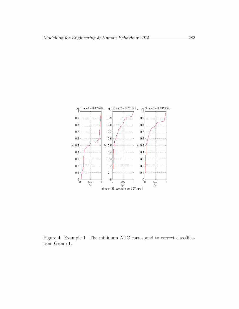
Modelling for Engineering & Human Behaviour 2015 283
Figure 4: Example 1. The minimum AUC correspond to correct classifica-tion, Group 1.
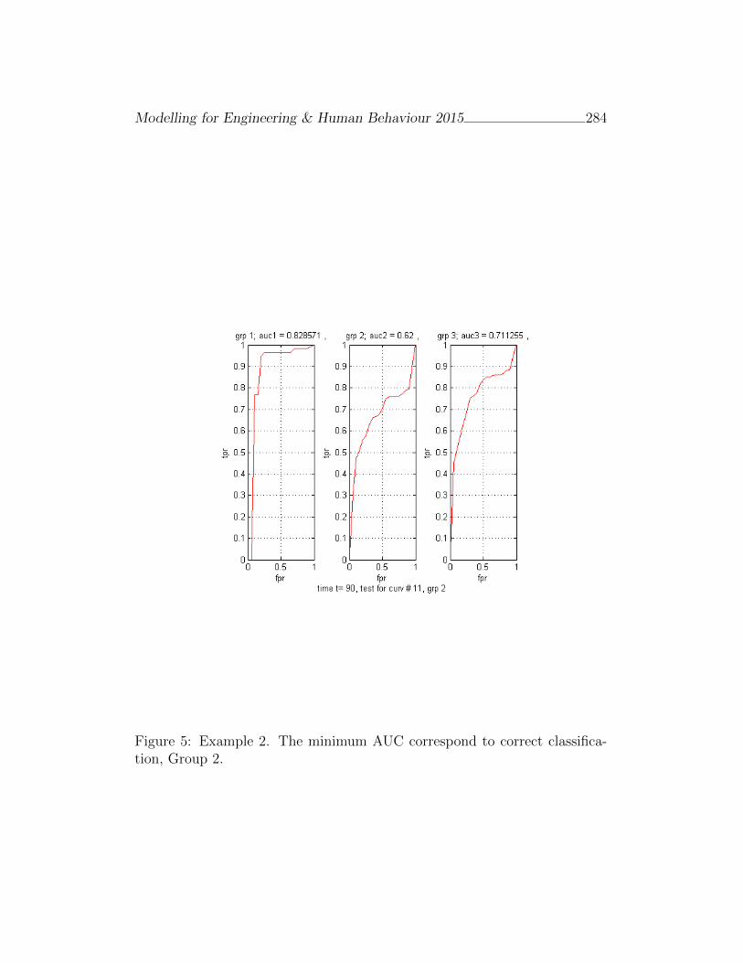
Modelling for Engineering & Human Behaviour 2015 284
Figure 5: Example 2. The minimum AUC correspond to correct classifica-tion, Group 2.
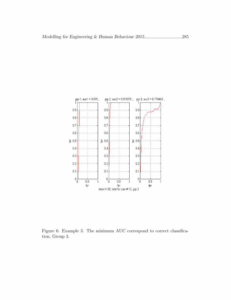
Modelling for Engineering & Human Behaviour 2015 285
Figure 6: Example 3. The minimum AUC correspond to correct classifica-tion, Group 3.
An approach for extrapolating turbocharger
compression ratio maps for engine simulations
J. Galindo, R. Navarro, L.M. Garcıa-Cuevas, and D. Tarı ∗
() CMT - Motores Termicos
Universitat Politecnica de Valencia
Camino de Vera, 46022 Valencia
November 30, 2015
1 Introduction
As pollutant regulations of internal combustion engines are becoming morerestrictive year by year, manufacturers are forced to design, certify and con-struct new engines as fast as possible. This rush combined with the highamount of independent variables and parameters available in the engine andits subsystems lead the characterization process to be simulated using 0D-1Dcodes, since the modern computational units are powerful enough to handlelarge number of simulations at the same time without risk of damaging actualengines. Thus, the improvement of the accuracy and convergence of the codesis critical.When a turbocharged ICE needs to be simulated, the most usedcompressor submodel in the 0D-1D codes relies on a compressor map wherethe operating condition is interpolated. This work is addressed to extend acommon compressor map range to assure the accuracy and convergence ofthe simulation.
Compressors behave quite differently in each of their regions, implying adifficulty for a single extrapolation method to predict all of them. So that,for the extrapolation approach proposed in this work, each zone is going to
∗e-mail: [email protected]
286
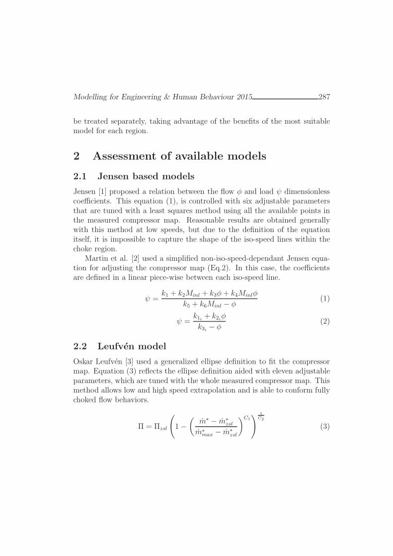
Modelling for Engineering & Human Behaviour 2015 287
be treated separately, taking advantage of the benefits of the most suitablemodel for each region.
2 Assessment of available models
2.1 Jensen based models
Jensen [1] proposed a relation between the flow φ and load ψ dimensionlesscoefficients. This equation (1), is controlled with six adjustable parametersthat are tuned with a least squares method using all the available points inthe measured compressor map. Reasonable results are obtained generallywith this method at low speeds, but due to the definition of the equationitself, it is impossible to capture the shape of the iso-speed lines within thechoke region.
Martin et al. [2] used a simplified non-iso-speed-dependant Jensen equa-tion for adjusting the compressor map (Eq.2). In this case, the coefficientsare defined in a linear piece-wise between each iso-speed line.
ψ =k1 + k2Minl + k3φ+ k4Minlφ
k5 + k6Minl − φ(1)
ψ =k1i + k2iφ
k3i − φ(2)
2.2 Leufven model
Oskar Leufven [3] used a generalized ellipse definition to fit the compressormap. Equation (3) reflects the ellipse definition aided with eleven adjustableparameters, which are tuned with the whole measured compressor map. Thismethod allows low and high speed extrapolation and is able to conform fullychoked flow behaviors.
Π = Πzsl
(1−
(m∗ − m∗
zsl
m∗
max− m∗
zsl
)C1
) 1
C2
(3)
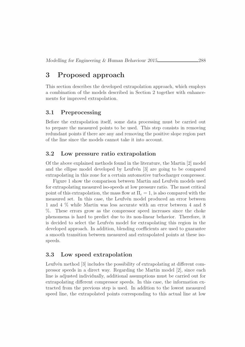
Modelling for Engineering & Human Behaviour 2015 288
3 Proposed approach
This section describes the developed extrapolation approach, which employsa combination of the models described in Section 2 together with enhance-ments for improved extrapolation.
3.1 Preprocessing
Before the extrapolation itself, some data processing must be carried outto prepare the measured points to be used. This step consists in removingredundant points if there are any and removing the positive slope region partof the line since the models cannot take it into account.
3.2 Low pressure ratio extrapolation
Of the above explained methods found in the literature, the Martin [2] modeland the ellipse model developed by Leufven [3] are going to be comparedextrapolating in this zone for a certain automotive turbocharger compressor.
Figure 1 show the comparison between Martin and Leufven models usedfor extrapolating measured iso-speeds at low pressure ratio. The most criticalpoint of this extrapolation, the mass flow at Πc = 1, is also compared with themeasured set. In this case, the Leufven model produced an error between1 and 4 % while Martin was less accurate with an error between 4 and 8%. These errors grow as the compressor speed increases since the chokephenomena is hard to predict due to its non-linear behavior. Therefore, itis decided to select the Leufven model for extrapolating this region in thedeveloped approach. In addition, blending coefficients are used to guaranteea smooth transition between measured and extrapolated points at these iso-speeds.
3.3 Low speed extrapolation
Leufven method [3] includes the possibility of extrapolating at different com-pressor speeds in a direct way. Regarding the Martin model [2], since eachline is adjusted individually, additional assumptions must be carried out forextrapolating different compressor speeds. In this case, the information ex-tracted from the previous step is used. In addition to the lowest measuredspeed line, the extrapolated points corresponding to this actual line at low
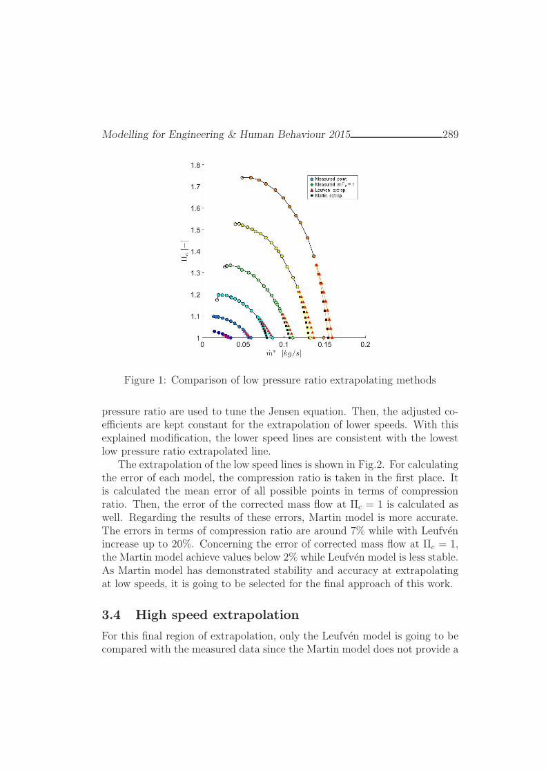
Modelling for Engineering & Human Behaviour 2015 289
Figure 1: Comparison of low pressure ratio extrapolating methods
pressure ratio are used to tune the Jensen equation. Then, the adjusted co-efficients are kept constant for the extrapolation of lower speeds. With thisexplained modification, the lower speed lines are consistent with the lowestlow pressure ratio extrapolated line.
The extrapolation of the low speed lines is shown in Fig.2. For calculatingthe error of each model, the compression ratio is taken in the first place. Itis calculated the mean error of all possible points in terms of compressionratio. Then, the error of the corrected mass flow at Πc = 1 is calculated aswell. Regarding the results of these errors, Martin model is more accurate.The errors in terms of compression ratio are around 7% while with Leufvenincrease up to 20%. Concerning the error of corrected mass flow at Πc = 1,the Martin model achieve values below 2% while Leufven model is less stable.As Martin model has demonstrated stability and accuracy at extrapolatingat low speeds, it is going to be selected for the final approach of this work.
3.4 High speed extrapolation
For this final region of extrapolation, only the Leufven model is going to becompared with the measured data since the Martin model does not provide a
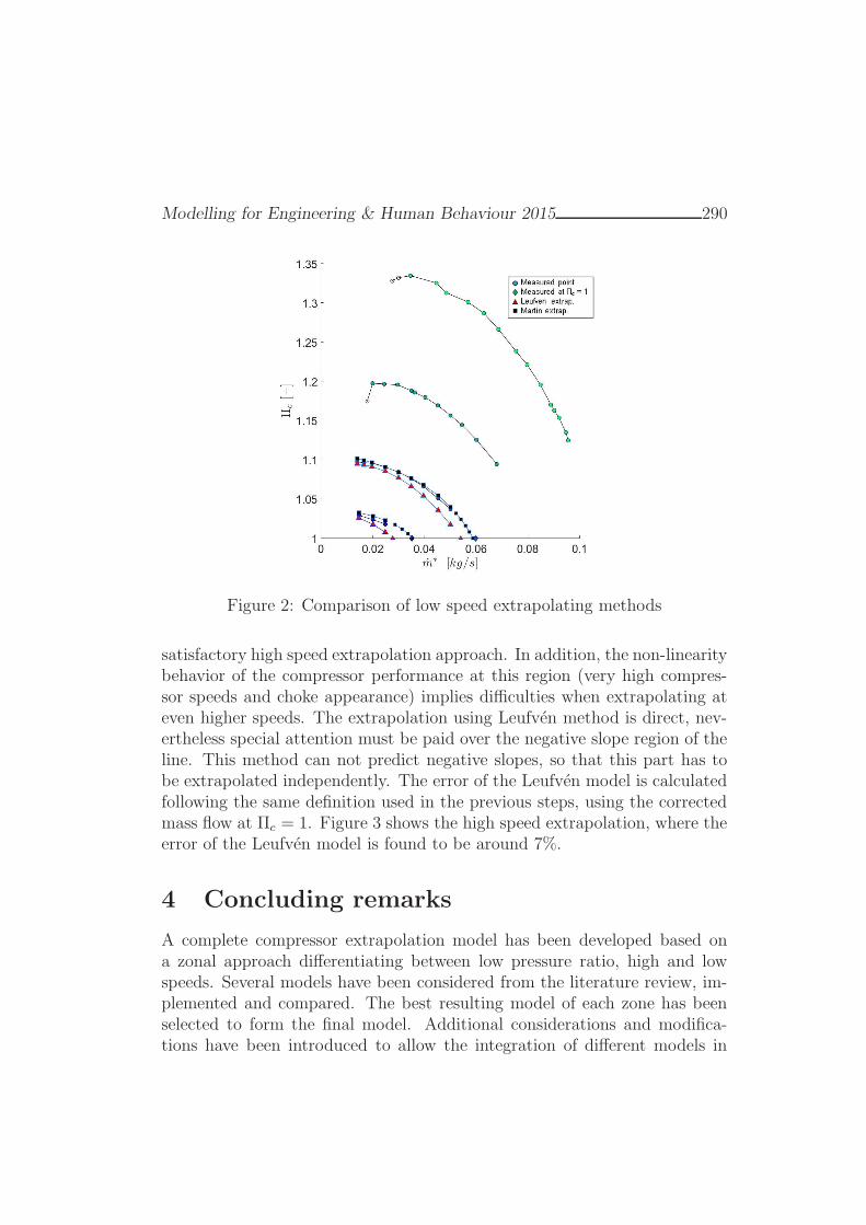
Modelling for Engineering & Human Behaviour 2015 290
Figure 2: Comparison of low speed extrapolating methods
satisfactory high speed extrapolation approach. In addition, the non-linearitybehavior of the compressor performance at this region (very high compres-sor speeds and choke appearance) implies difficulties when extrapolating ateven higher speeds. The extrapolation using Leufven method is direct, nev-ertheless special attention must be paid over the negative slope region of theline. This method can not predict negative slopes, so that this part has tobe extrapolated independently. The error of the Leufven model is calculatedfollowing the same definition used in the previous steps, using the correctedmass flow at Πc = 1. Figure 3 shows the high speed extrapolation, where theerror of the Leufven model is found to be around 7%.
4 Concluding remarks
A complete compressor extrapolation model has been developed based ona zonal approach differentiating between low pressure ratio, high and lowspeeds. Several models have been considered from the literature review, im-plemented and compared. The best resulting model of each zone has beenselected to form the final model. Additional considerations and modifica-tions have been introduced to allow the integration of different models in
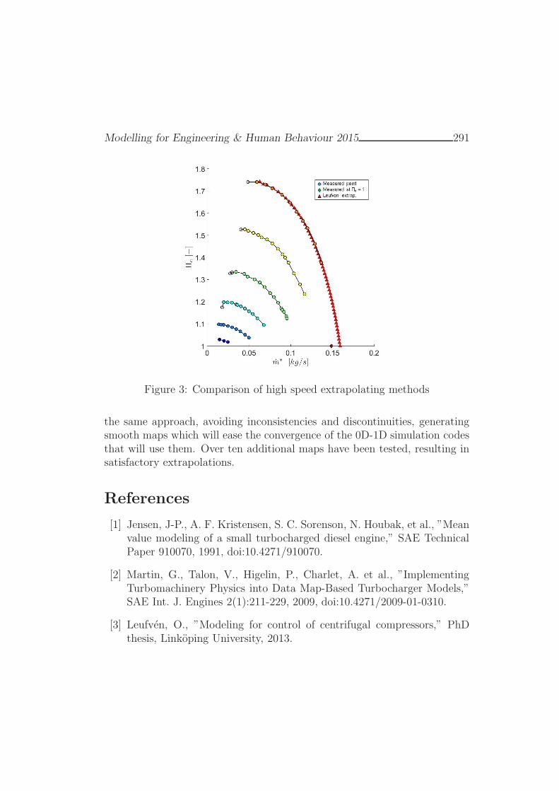
Modelling for Engineering & Human Behaviour 2015 291
Figure 3: Comparison of high speed extrapolating methods
the same approach, avoiding inconsistencies and discontinuities, generatingsmooth maps which will ease the convergence of the 0D-1D simulation codesthat will use them. Over ten additional maps have been tested, resulting insatisfactory extrapolations.
References
[1] Jensen, J-P., A. F. Kristensen, S. C. Sorenson, N. Houbak, et al., ”Meanvalue modeling of a small turbocharged diesel engine,” SAE TechnicalPaper 910070, 1991, doi:10.4271/910070.
[2] Martin, G., Talon, V., Higelin, P., Charlet, A. et al., ”ImplementingTurbomachinery Physics into Data Map-Based Turbocharger Models,”SAE Int. J. Engines 2(1):211-229, 2009, doi:10.4271/2009-01-0310.
[3] Leufven, O., ”Modeling for control of centrifugal compressors,” PhDthesis, Linkoping University, 2013.
The inverse problem associated toK, s + 1-potent matrices
L. Lebtahi[ ∗, O. Romero† †, and N. Thome‡ ‡
([) Universidad Internacional de La Rioja, E–26002 Logrono, Spain,
(†) Departamento de Comunicaciones,
Universitat Politecnica de Valencia, E–46022 Valencia, Spain,
(‡) Instituto Universitario de Matematica Multidisciplinar,
Universitat Politecnica de Valencia, E–46022 Valencia, Spain.
November 30, 2015
1 Introduction
In [3], the authors introduced and characterized a new kind of matrices calledK, s+ 1-potent where K is involutory. We recall that a matrix A ∈ Cn×n
is called K, s + 1-potent if KAs+1K = A and for some s ∈ 1, 2, . . . .These matrices generalize all the following classes of matrices: s+1-potentmatrices, periodic matrices, idempotent matrices, involutory matrices, cen-trosymmetric matrices, mirrorsymmetric matrices, circulant matrices, etc.The class of K, s+ 1-potent matrices was linked to other kind of matricessuch as s+ 1-generalized projectors, K-Hermitian matrices, normal ma-trices, Hamiltonian matrices, etc. [4]. Moreover, some related results weregiven in [1] from an algebraic point of view. Furthermore, in [5] the authorsdeveloped an algorithm to perform this class of matrices. This problem iscalled the direct problem.
∗e-mail: [email protected]†e-mail: [email protected]‡e-mail: [email protected]
292
Modelling for Engineering & Human Behaviour 2015 293
The aim of this paper is to design an algorithm to solve the inverse prob-lem, that is, to find all the involutory matrices K for which a given matrixA is K, s+ 1-potent.
2 Obtaining the involutory matrices K
It is well known that the Kronecker product is an important tool to solve somematrix problems, as for example the Sylvester and Lyapunov equations. TheKronecker sum, obtained as a sum of two Kronecker products, is applied, forexample, to solve the two-dimensional heat equation, to rewrite the Jacobiiteration matrix, etc. [6]. The notations ⊗ and ⊕ used in this paper refer tothe Kronecker product and Kronecker sum of two matrices, respectively; andXT denotes the transpose of the matrix X [2]. For any matrix X = [xij] ∈Cn×n, let v(X) = [vk] ∈ Cn2×1 be the vector formed by stacking the columnsof X into a single column vector. The expression [v(X)](j−1)n+1,...,(j−1)n+n,for j = 1, . . . , n, denotes the jth column of X.
In what follows, we will need the following property: if A ∈ Cn×n andB ∈ Cn×n then
Ker(A) ∩Ker(B) = Ker
([AB
]), (1)
which is also valid for a finite number of matrices of suitable sizes, whereKer(.) denotes the null space of the matrix (.).
We recall that the principal idempotents associated with the eigenvaluesλ1, . . . , λl are given by
Pt =pt(A)
pt(λt)where pt(η) =
l∏i = 1i 6= t
(η − λi). (2)
By using the function ϕ and the projectors introduced in [3], it is possible toconsider the matrix
M =
P T0 ⊕−Pϕ(0)
P T1 ⊕−Pϕ(1)
...P T(s+1)2−2 ⊕−Pϕ((s+1)2−2)
P T(s+1)2−1 ⊕−P(s+1)2−1
. (3)
The algorithm presented below solves the aforementioned inverse problem.

Modelling for Engineering & Human Behaviour 2015 294
Algorithm
Inputs: A matrix A ∈ Cn×n and an integer s ≥ 1.
Outputs: All the involutory matrices K ∈ Cn×n such that A is aK, s+ 1-potent matrix.
Step 1 Compute σ(A) = σ1, σ2, . . . , σl.
Step 2 Define Λ = 0 ∪ Ω(s+1)2−1 = λ0, λ1, . . . , λ(s+1)2−1 in
the following order 0, ω1(s+1)2−1, . . . , ω
(s+1)2−2(s+1)2−1, 1.
Step 3 If σi /∈ Λ for some i ∈ 1, 2, . . . , l or A(s+1)2 6= A thengo to Step 13.
Step 4 Rearrange the eigenvalues σi’s as in Λ. Rename them byβ1, β2, . . . , βl.
Step 5 For every i = 1, 2, . . . , l, identify βi with the correspond-ing λj, for all j = 0, 1, . . . , (s + 1)2 − 1. The set of thesesubscripts j’s will be called j1, j2, . . . , jl.
Step 6 For every t ∈ 1, 2, . . . , l, compute the principal idem-potents associated with λj1 , λj2 , . . . , λjl by using (2).
Step 7 Compute ϕ(j1), ϕ(j2), . . . , ϕ(jl).
Step 8 Define the matrix M as in (3) containing only the rowblocks corresponding to the eigenvalues λj1 , λj2 , . . . , λjl.
Step 9 Compute the null space of the matrix M obtaining thesolution v(K).
Step 10 If v(K) = 0 then go to Step 13.
Step 11 Reshape the entries of v(K) in the square matrix Kobtaining
K =[
[v(K)]1,...,n [v(K)]n+1,...,2n . . . [v(K)](n2−n+1,...,n2]
Step 12 The outputs are those matricesK’s that satisfyK2 = In.Go to End. Otherwise, go to Step 13.
Modelling for Engineering & Human Behaviour 2015 295
Step 13 ‘There is no matrix K ∈ Cn×n such that A is K, s+1-potent’.
End
Example 1 For s = 4 and
A =
i 0 00 5 −20 15 −6
our algorithm gives all the following solutions K:
K =
z9 0 00 −5z1 + 6z5 2z1 − 2z50 −15z1 + 15z5 6z1 − 5z5
,where z1, z5, z9 ∈ −1, 1.
References
[1] G. Bourgeois Similar powers of a matrix Linear and Multilinear Algebra,(61): 699–709, 2013.
[2] P. Lancaster, The Theory of Matrices, 2nd Edition. London, AcademicPress, 1985.
[3] L. Lebtahi, O. Romero, N. Thome, Characterizations of K, s + 1-Potent Matrices and Applications Linear Algebra and its Applications,(436): 293-306, 2012.
[4] L. Lebtahi, O. Romero, N. Thome, Relations between K, s+1-PotentMatrices and Different Classes of Complex Matrices Linear Algebra andits Applications, (438): 1517–1531, 2013.
[5] L. Lebtahi, O. Romero, N. Thome, Algorithms for K, s+1-potent ma-trix constructions Journal of Computational and Applied Mathematics,(249): 157–162, 2013.
[6] D.S. Watkins, Fundamentals of Matrix Computations, 3rd Edition. NewJersey, Wiley, 2010.
High-order iterative methods for solvingnonlinear models ∗
A. Cordero[, A. Franques[, and Juan R. Torregrosa[ †
([) Instituto de Matematicas Multidisciplinar,
Universitat Politecnica de Valencia, Camino de Vera, s/n, 46022-Valencia, Spain
November 30, 2015
1 Introduction
The polar decomposition is a generalization to complex matrices of the trigono-metric representation of a complex number. Specifically, let A be a complexmatrix of size m × n, m ≥ n (in other case, we work with the transposematrix). Then there exist a matrix U ∈ Cm×n, with orthonormal columnsand a Hermitian positive semi-definite H ∈ Cn×n such that
A = UH, U∗U = In, (1)
where U∗ denotes the conjugate transpose of U and In is the identity matrixof size n×n. The Hermitian factor H is always unique and can be expressedas H = (A∗A)1/2. If matrix A has full rank, then H is positive definite andthe unitary factor U is uniquely determined. The polar decomposition is wellknown and can be found in many textbooks, see, for example, [4].
Let us observe that, once the unitary factor U is calculated, the otherfactor is obtained in a simple way, H = U∗A. So, our goal in this work is toobtain factor U .
∗This research was partially supported by Ministerio de Economıa y CompetitividadMTM2014-52016-C2-2-P.†e-mail: [email protected]
296
Modelling for Engineering & Human Behaviour 2015 297
In this paper, we are interested in computing the polar decompositionby means of an iterative method of the fixed-point form Uk+1 = G(Uk),provided that the initial guess matrix U0 is given. Let us remember thatfrom the unitary factor U the other factor of the polar decomposition isobtained easily. In [3] Higham proposed a fixed-point algorithm based onNewton’s method to compute the square root of a number, for obtaining theunitary factor U of a nonsingular n×n matrix A. Starting with U0 = A, thesequence Uk is computed by
Uk+1 =1
2(Uk + U−∗k ), (2)
where U−∗k denotes (U−1k )∗. The quadratic convergence of sequence Ukk≥0was proved.
Fifteen years later, Du in [1] generalized Higham’s algorithm for rectan-gular matrices by means of the iterative expression
Uk+1 =1
2(Uk + U †∗k ), (3)
where U †k denotes the Moore-Penrose pseudoinverse of Uk. This scheme keepsthe order of convergence of the previous one.
In a similar way as Hihgam with Newton’s method, Gander in [2] usedHalley’s scheme for scalar equations for designing the following algorithmthat converges to the unitary factor with order of convergence three for non-singular matrices.
Uk+1 = [Uk(3I + U∗kUk)] [I + 3U∗kUk]−1 . (4)
Recently, a fourth-order iterative method for computing the polar decom-position was developed by Khaksar and Soleymani in [5] from a fourth-ordermethod for solving nonlinear equations. The iterative expression of thisscheme is
Uk+1 = [Uk(7I + Yk)(I + 3Yk)] [I + 18Yk + 13Zk]−1 , (5)
where Yk = U∗kUk, Zk = YkYk and U0 = A.The rest of the paper is organized as follows: in Section 2, a new root-
finding scheme for scalar equations is designed and, from it, an iterativescheme for computing the polar decomposition of any rectangular matrix is
Modelling for Engineering & Human Behaviour 2015 298
derived. The sixth-order of convergence, for as proper initial matrix, of thedesigned method is proving. Some numerical test are presented in Section 3to confirm the theoretical results and for comparing our scheme with otherknown ones.
2 The proposed iterative scheme and its con-
vergence
Many multi-point iterative schemes for solving nonlinear scalar equationsf(x) = 0 have been designed in the last years. The main interest of thesefixed-point methods is the possibility to reach any order of convergence. Theconnection between the matrix iterations for computing polar decomposition,or in general for approximating the solution of a nonlinear matrix equation,and iterative methods for nonlinear scalar equations were described by Ian-nazzo in [6].
In fact, the matrix form of fixed-point type methods for polar decompo-sition is the generalization of applying the nonlinear equation solvers to thematrix equation
F (U) := U∗U − I = 0,
where I is the identity matrix of the appropriate size. This reveals therelation between the polar decomposition and matrix sign function.
Let us consider the following iterative expression for finding the simplezeros of a nonlinear equation f(x) = 0
yk = xk −10− 4Lf (xk)
10− 9Lf (xk)
f(xk)
f ′(xk),
xk+1 = yk −f(yk)
f ′(yk),
(6)
where Lf (xk) =f(xk)f ′′(xk)
f ′(xk)2is the degree of logarithmic convexity. This
scheme is the composition of the scheme proposed in [7] for finding matrixsign functions and Newton’s method. By using Taylor expansion of thedifferent elements of the iterative expression (6), we can prove the followingresult.
Theorem 1 Let α ∈ I be a simple zero of a sufficiently differentiable func-tion f : I ⊆ R → R for an open interval I, and x0 ∈ I an initial guess
Modelling for Engineering & Human Behaviour 2015 299
close enough to α. Then, iterative expression (6) converge to α with order ofconvergence six, being its error equation
ek+1 =1
25c2(c
22 − 5c3)
2e6k +O(e7k),
where cj =1
j!
f (j)(α)
f ′(α), j = 2, 3, . . ., and ek = xk − α.
Solving the equation u2 − 1 = 0 by (6), we have the iterative expressionin the reciprocal form
uk+1 =36uk + 314u3k + 384u5k + 66u7k
4 + 141u2k + 435u4k + 211u6k + 9u8k, k = 0, 1, . . . (7)
The global convergence of this iterative formula on quadratic polynomialsallows us to extend it in the matrix form
Uk+1 = [Uk(36I + 314Yk + 384Zk + 66Xk)] [4 + 141Yk + 435Zk + 211Xk + 9Wk]−1 ,(8)
where Yk = U∗kUk, Zk = YkYk, Xk = YkZk and Wk = ZkZk.Expression (8) is a new iterative fixed-point scheme for finding the polar
decomposition via calculating the unitary matrix U . In the following resultwe analyze the convergence of sequence Ukk≥0 generated by the iterativescheme (8).
Theorem 2 Let A be an arbitrary m × n complex matrix of rank r. Then,the sequence of matrix iterates Ukk≥0 obtained from (8) converges to theunitary factor U , with order of convergence six, for U0 = A.
3 Numerical results
In this section we are going to present the numerical results. The numericaltests have been made in Matlab in double precision arithmetics, with 50digits of mantissa. The computer specifications are Intel(R) Core(TM), i5-2500, CPU 3.30 GHz, with 16 GB of RAM. We compare our scheme, denotedas CTM, with several known iterative methods such as (3) denoted by NM,(4) denoted by HM and (5) denoted by KSM, of orders of convergence two,

Modelling for Engineering & Human Behaviour 2015 300
three and four, respectively, which also require one inverse per iteration. Weuse two different stopping criterium: the difference between the last iterates
‖Uk+1 − Uk‖M < tol
and this other one ∥∥U∗k+1Uk+1 − I∥∥M< tol,
where tol is the tolerance and ‖ · ‖M is a proper matrix norm.
Example 1 In this experiment, we analyze the behavior of the differentmethods on a random rectangular matrix of size 510 × 500 generated inMatlab by A = rand(510, 500), working in double precision arithmetics.
In Table 1 we show the results obtained by applying the different methodson matrix A, with tolerance tol = 10−10 and initial estimation U0 = A.Specifically, we present the values of ‖Uk+1−Uk‖2 and ‖UT
k+1Uk+1− I500‖2 inthe last iteration, where I500 is the identity matrix of order 500, the numberof iterations and the elapsed time, in seconds, being the mean execution timefor 50 performances of each method (the command cputime of Matlab hasbeen used).
Newton Halley KSM CTMiterations 13 9 7 6‖Uk+1 − Uk‖2 1.70e-14 1.12e-15 1.64e-14 1.31e-15‖UT
k+1Uk+1 − I500‖2 3.34e-15 1.50e-15 1.51e-15 1.31e-15e-time 5.67 1.93 1.84 1.78
Table 1: Numerical results for a random matrix of size 510 × 500 in doubleprecision aritmethics
Example 2 In this example, we analyze the behavior of the different meth-ods on Hilbert matrix of size 75× 75 generated in Matlab by B = hilb(75),working in double precision arithmetics and under the same conditions asExample 1. Let us remember that it is an example of ill-conditioned matrix.
In this case, the number of iterations increases significantly, in fact New-ton’s method is not convergent. However, the elapsed time decreases becausematrix B has a small size.
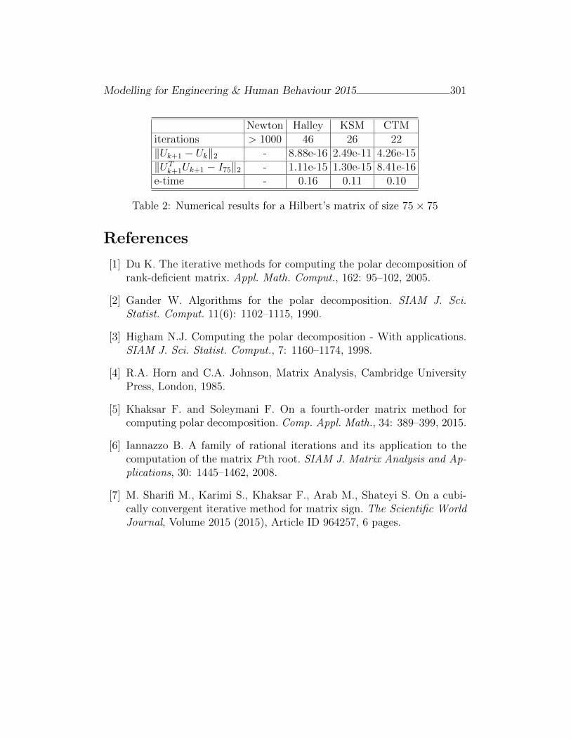
Modelling for Engineering & Human Behaviour 2015 301
Newton Halley KSM CTMiterations > 1000 46 26 22‖Uk+1 − Uk‖2 - 8.88e-16 2.49e-11 4.26e-15‖UT
k+1Uk+1 − I75‖2 - 1.11e-15 1.30e-15 8.41e-16e-time - 0.16 0.11 0.10
Table 2: Numerical results for a Hilbert’s matrix of size 75× 75
References
[1] Du K. The iterative methods for computing the polar decomposition ofrank-deficient matrix. Appl. Math. Comput., 162: 95–102, 2005.
[2] Gander W. Algorithms for the polar decomposition. SIAM J. Sci.Statist. Comput. 11(6): 1102–1115, 1990.
[3] Higham N.J. Computing the polar decomposition - With applications.SIAM J. Sci. Statist. Comput., 7: 1160–1174, 1998.
[4] R.A. Horn and C.A. Johnson, Matrix Analysis, Cambridge UniversityPress, London, 1985.
[5] Khaksar F. and Soleymani F. On a fourth-order matrix method forcomputing polar decomposition. Comp. Appl. Math., 34: 389–399, 2015.
[6] Iannazzo B. A family of rational iterations and its application to thecomputation of the matrix P th root. SIAM J. Matrix Analysis and Ap-plications, 30: 1445–1462, 2008.
[7] M. Sharifi M., Karimi S., Khaksar F., Arab M., Shateyi S. On a cubi-cally convergent iterative method for matrix sign. The Scientific WorldJournal, Volume 2015 (2015), Article ID 964257, 6 pages.
Implementation/Adaptation of a Total
Variation Diminishing (TVD) scheme to a
non-linear 1D finite volume method for engine
gas-exchange modelling
A.J. Torregrosa∗, A. Broatch, F.J. Arnau, and M. HernandezCMT - Motores Termicos. Universitat Politecnica de Valencia.
Camino de Vera s/n. 46022–Valencia, Spain.
November 30, 2015
1 Introduction
A suitable compromise between the quality of the solution and the compu-tational cost when predicting wave dynamics in intake and exhaust systemsof internal combustion engines is provided by quasi-3D models, in which themomentum equation is solved in a simplified fashion on a staggered mesh [1].However, those methods are affected by overshoots at discontinuities whenused in their basic form. It was shown in previous work by the authors [2]that a Flux Corrected Transport (FCT) methodology provided satisfactoryresults through the combination of dissipation via damping together withthe phoenical form of the anti-diffusion term. However, FCT methods candistort the solution and produce significant errors in mass conservation un-der some circumstances, and thus flux limiters based on the total variationdiminishing (TVD) criterion [3] are usually preferred.
In this paper, the benefits of rendering the quasi-3D model equations inTVD form were explored, both in terms of the removal of flow oscillationsand of the quality of the frequency domain behaviour of the solution.
∗e-mail: [email protected]
302
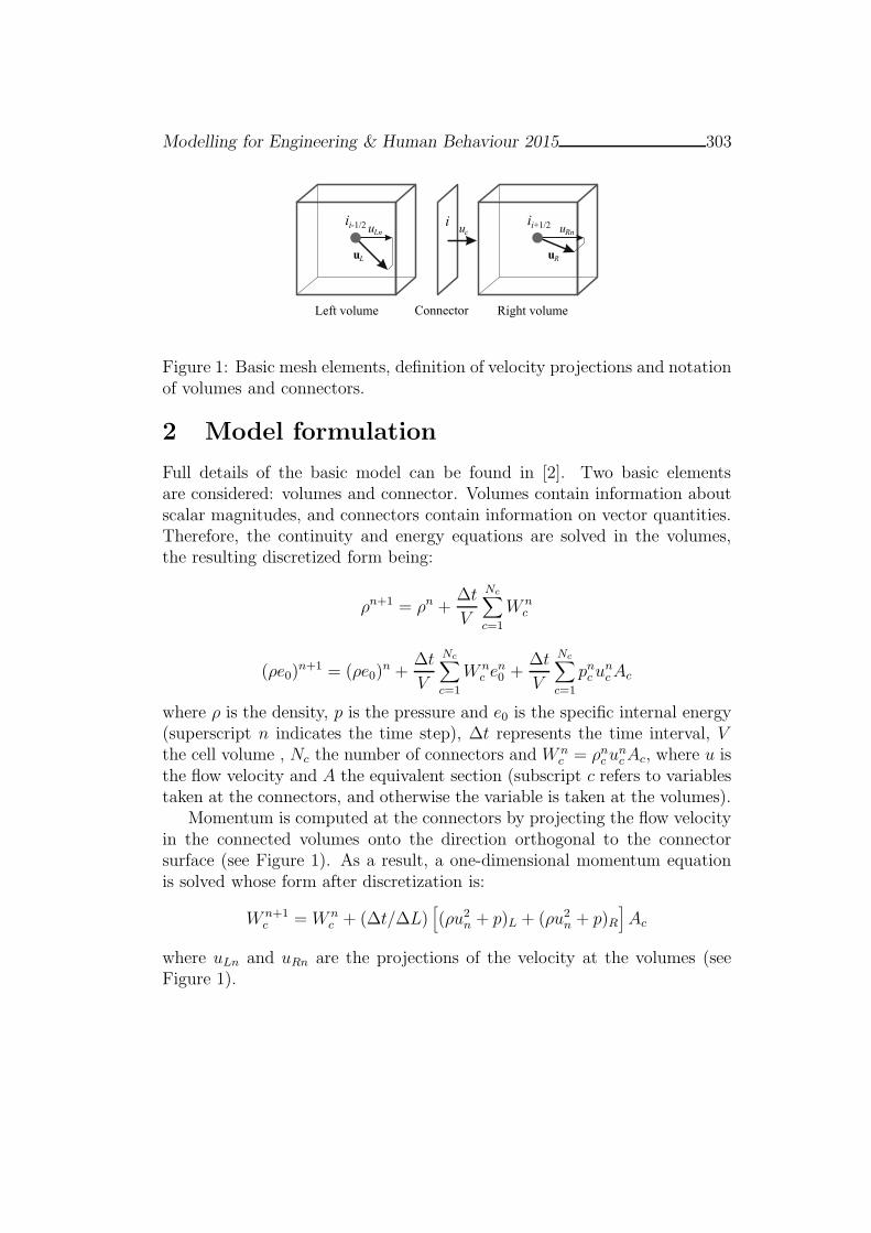
Modelling for Engineering & Human Behaviour 2015 303
uRnucuLn
uL uR
Connector Right volumeLeft volume
iii-1/2 ii+1/2
Figure 1: Basic mesh elements, definition of velocity projections and notationof volumes and connectors.
2 Model formulation
Full details of the basic model can be found in [2]. Two basic elementsare considered: volumes and connector. Volumes contain information aboutscalar magnitudes, and connectors contain information on vector quantities.Therefore, the continuity and energy equations are solved in the volumes,the resulting discretized form being:
ρn+1 = ρn +∆t
V
Nc∑
c=1
W n
c
(ρe0)n+1 = (ρe0)
n +∆t
V
Nc∑
c=1
W n
c en
0+
∆t
V
Nc∑
c=1
pncun
cAc
where ρ is the density, p is the pressure and e0 is the specific internal energy(superscript n indicates the time step), ∆t represents the time interval, Vthe cell volume , Nc the number of connectors and W n
c= ρn
cun
cAc, where u is
the flow velocity and A the equivalent section (subscript c refers to variablestaken at the connectors, and otherwise the variable is taken at the volumes).
Momentum is computed at the connectors by projecting the flow velocityin the connected volumes onto the direction orthogonal to the connectorsurface (see Figure 1). As a result, a one-dimensional momentum equationis solved whose form after discretization is:
W n+1
c= W n
c+ (∆t/∆L)
[(ρu2
n+ p)L + (ρu2
n+ p)R
]Ac
where uLn and uRn are the projections of the velocity at the volumes (seeFigure 1).
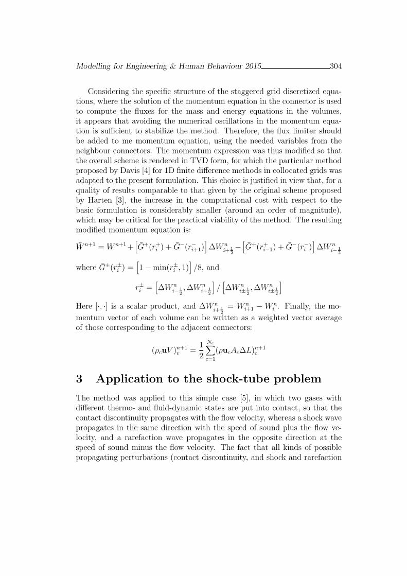
Modelling for Engineering & Human Behaviour 2015 304
Considering the specific structure of the staggered grid discretized equa-tions, where the solution of the momentum equation in the connector is usedto compute the fluxes for the mass and energy equations in the volumes,it appears that avoiding the numerical oscillations in the momentum equa-tion is sufficient to stabilize the method. Therefore, the flux limiter shouldbe added to me momentum equation, using the needed variables from theneighbour connectors. The momentum expression was thus modified so thatthe overall scheme is rendered in TVD form, for which the particular methodproposed by Davis [4] for 1D finite difference methods in collocated grids wasadapted to the present formulation. This choice is justified in view that, for aquality of results comparable to that given by the original scheme proposedby Harten [3], the increase in the computational cost with respect to thebasic formulation is considerably smaller (around an order of magnitude),which may be critical for the practical viability of the method. The resultingmodified momentum equation is:
W n+1 = W n+1+[G+(r+i ) + G−(r−i+1
)]∆W n
i+1
2
−[G+(r+i−1
) + G−(r−i )]∆W n
i−1
2
where G±(r±i ) =[1−min(r±i , 1)
]/8, and
r±i=
[∆W n
i−1
2
,∆W n
i+1
2
]/[∆W n
i±1
2
,∆W n
i±1
2
]
Here [·, ·] is a scalar product, and ∆W n
i+1
2
= W n
i+1− W n
i . Finally, the mo-
mentum vector of each volume can be written as a weighted vector averageof those corresponding to the adjacent connectors:
(ρcuV )n+1
v=
1
2
Nc∑
c=1
(ρucAc∆L)n+1
c
3 Application to the shock-tube problem
The method was applied to this simple case [5], in which two gases withdifferent thermo- and fluid-dynamic states are put into contact, so that thecontact discontinuity propagates with the flow velocity, whereas a shock wavepropagates in the same direction with the speed of sound plus the flow ve-locity, and a rarefaction wave propagates in the opposite direction at thespeed of sound minus the flow velocity. The fact that all kinds of possiblepropagating perturbations (contact discontinuity, and shock and rarefaction
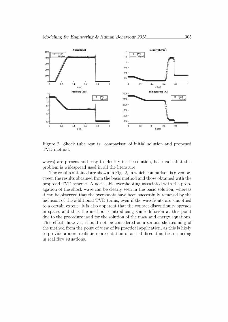
Modelling for Engineering & Human Behaviour 2015 305
Figure 2: Shock tube results: comparison of initial solution and proposedTVD method.
waves) are present and easy to identify in the solution, has made that thisproblem is widespread used in all the literature.
The results obtained are shown in Fig. 2, in which comparison is given be-tween the results obtained from the basic method and those obtained with theproposed TVD scheme. A noticeable overshooting associated with the prop-agation of the shock wave can be clearly seen in the basic solution, whereasit can be observed that the overshoots have been successfully removed by theinclusion of the additional TVD terms, even if the wavefronts are smoothedto a certain extent. It is also apparent that the contact discontinuity spreadsin space, and thus the method is introducing some diffusion at this pointdue to the procedure used for the solution of the mass and energy equations.This effect, however, should not be considered as a serious shortcoming ofthe method from the point of view of its practical application, as this is likelyto provide a more realistic representation of actual discontinuities occurringin real flow situations.
Modelling for Engineering & Human Behaviour 2015 306
4 Conclusion
A staggered-mesh time domain model which makes use of a non-linear sec-ond order time and space discretization based on finite volumes has beencomplemented with suitable terms so that a Total Variation Diminishingformulation has been achieved. This has allowed suppressing overshoots atdiscontinuities. However, the behaviour of the solution in the vicinity of thediscontinuities present in the shock-tube problem indicates that additionalwork is needed so that the dissipative character of the method may be re-duced.
References
[1] G. Montenegro, A. Onorati and A. Della Torre. The prediction of si-lencer acoustical performances by 1D, 1D-3D and quasi-3D non-linearapproaches. Computers & Fluids, 71: 208–223, 2013.
[2] A.J. Torregrosa, A. Broatch, F.J. Arnau and M. Hernandez. A non-linear quasi-3D model with Flux-Corrected-Transport for engine gas-exchange modelling. Journal of Computational and Applied Mathemat-
ics, 291: 103-111, 2016.
[3] A. Harten. High resolution schemes for hyperbolic conservation laws.Journal of Computational Physics, 49: 357–393, 1983.
[4] S.F. Davis. A simplified TVD finite difference scheme via artificial vis-cosity. SIAM Journal on Scientific and Statistical Computing, 8: 1–18,1987.
[5] G.A. Sod. Survey of several finite-difference methods for systems of non-linear hyperbolic conservation laws. Journal of Computational Physics,135: 172–186, 1997.
Modelling for Engineering & Human Behaviour 2015________________________307
Vibrations induced on the railway structure by the vehicle
passage on a turnout. Study of mitigation measures
J. L. Velarte1*
, A. E. Blanco1, S. Morales
1, J. Real
1
1Institute for Multidisciplinary Mathematics, Polytechnic University of Valencia,
46022, Valencia, Spain
November 30, 2015
1. Introduction
A turnout is a simple mechanism that allows the intersection of two different tracks at
the same level. Nevertheless, the presence of singular points such as crossing noses or
switch blades hinders its dynamic behavior. The main reason lies in the rail geometry
variations, which induces irregularities in the wheel-rail contact. As a consequence,
great dynamic forces take place [1] which damage both vehicle and track elements and
force to the railway operator to adopt expensive corrective measures.
In order to delve into this topic, this investigation studies the vertical dynamic response
of a railway turnout once some corrective measures are introduced. For this purpose, a
numerical feed-back interaction between a Finite Elements model of the track and a
multi-body model of the vehicle is developed. Then, the results of both models are
coupled and the validity of the whole process is assessed with real data obtained during
a data gathering campaign.
2. Methodology
In order to assess the influence of different corrective measures in the vibration
generation phenomenon, a numerical feed-back interaction between a Finite Elements
model of a track developed by means of ANSYS software and a multi-body model of a
rail vehicle developed by means of VAMPIRE software is proposed (Figure 1).
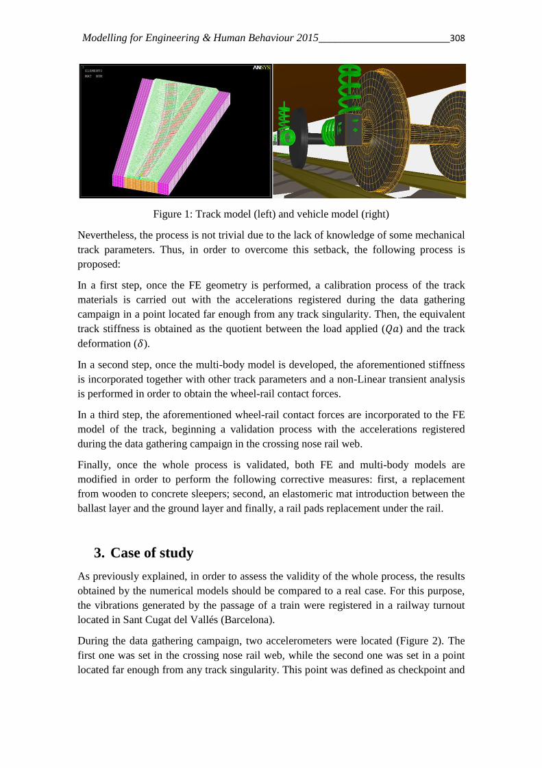
Modelling for Engineering & Human Behaviour 2015________________________308
Figure 1: Track model (left) and vehicle model (right)
Nevertheless, the process is not trivial due to the lack of knowledge of some mechanical
track parameters. Thus, in order to overcome this setback, the following process is
proposed:
In a first step, once the FE geometry is performed, a calibration process of the track
materials is carried out with the accelerations registered during the data gathering
campaign in a point located far enough from any track singularity. Then, the equivalent
track stiffness is obtained as the quotient between the load applied (𝑄𝑎) and the track
deformation (𝛿).
In a second step, once the multi-body model is developed, the aforementioned stiffness
is incorporated together with other track parameters and a non-Linear transient analysis
is performed in order to obtain the wheel-rail contact forces.
In a third step, the aforementioned wheel-rail contact forces are incorporated to the FE
model of the track, beginning a validation process with the accelerations registered
during the data gathering campaign in the crossing nose rail web.
Finally, once the whole process is validated, both FE and multi-body models are
modified in order to perform the following corrective measures: first, a replacement
from wooden to concrete sleepers; second, an elastomeric mat introduction between the
ballast layer and the ground layer and finally, a rail pads replacement under the rail.
3. Case of study
As previously explained, in order to assess the validity of the whole process, the results
obtained by the numerical models should be compared to a real case. For this purpose,
the vibrations generated by the passage of a train were registered in a railway turnout
located in Sant Cugat del Vallés (Barcelona).
During the data gathering campaign, two accelerometers were located (Figure 2). The
first one was set in the crossing nose rail web, while the second one was set in a point
located far enough from any track singularity. This point was defined as checkpoint and

Modelling for Engineering & Human Behaviour 2015________________________309
was located 11 meters far from the crossing nose and 31 meters far from the switch
blades. The registered vehicle was a CAF 112 and circulated through the main direction.
Figure 2: Studied stretch (left) and crossing nose accelerometer location (right)
4. Model’s development
The computational considerations of both models are summarized below.
- FEM model:
The track geometry is simplified according to [2]. Thus, hexahedral SOLID45 elements
are set in rail pads, sleepers, ballast layer, ground layer and reinforced concrete layer.
Nonetheless, in order to simplify the rails geometry and in order to consider the rails
inertia variations, linear BEAM4 elements are considered for rails. In this sense, the
area moment of inertia of each section is obtained by means of AutoCAD software by
defining the 2-Dimensional geometry.
For the simulation, a succession of punctual forces is performed as if the vehicle
circulation were. Thus, the dynamic Eq. (1) is solved in every node of the model. In this
equation, [M], [C] and [K] are the mass, damping and stiffness matrixes; 𝑢, and are
the displacements, velocities and accelerations vectors and F(t) is the external forces
vector.
[M]+[C]+[K]𝑢=F(t) (1)
To calculate the damping matrix, it has been considered the Rayleigh’s damping theory
by assuming that [C] depends on two coefficients 𝛼 and 𝛽 according to Eq. (2).
[C] = α*[M] + β*[K] (2)
The diagonalization of this matrix allows obtaining the i-th term in the diagonal from
Eq. (3), where [Ø] is the normalized eigenvector of the mass matrix and wi is the natural
frequency of the system.
[Ø]𝑇[C][Ø] = α[Ø]T[M][Ø] + β[Ø]T[K][Ø] = [C] = [𝛼 + 𝛽𝑤1
2 … 0⋮ ⋱ ⋮0 … 𝛼 + 𝛽𝑤𝑛
2] (3)
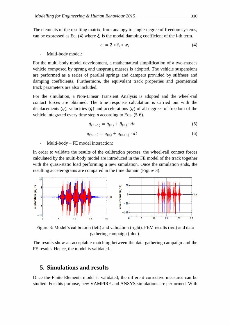
Modelling for Engineering & Human Behaviour 2015________________________310
The elements of the resulting matrix, from analogy to single-degree of freedom systems,
can be expressed as Eq. (4) where 𝜉𝑖 is the modal damping coefficient of the i-th term.
𝑐𝑖 = 2 ∗ 𝜉𝑖 ∗ 𝑤𝑖 (4)
- Multi-body model:
For the multi-body model development, a mathematical simplification of a two-masses
vehicle composed by sprung and unsprung masses is adopted. The vehicle suspensions
are performed as a series of parallel springs and dampers provided by stiffness and
damping coefficients. Furthermore, the equivalent track properties and geometrical
track parameters are also included.
For the simulation, a Non-Linear Transient Analysis is adopted and the wheel-rail
contact forces are obtained. The time response calculation is carried out with the
displacements (𝑞), velocities () and accelerations () of all degrees of freedom of the
vehicle integrated every time step n according to Eqs. (5-6).
(𝑛+1) = (𝑛) + (𝑛) · 𝑑𝑡 (5)
𝑞(𝑛+1) = 𝑞(𝑛) + (𝑛+1) · 𝑑𝑡 (6)
- Multi-body – FE model interaction:
In order to validate the results of the calibration process, the wheel-rail contact forces
calculated by the multi-body model are introduced in the FE model of the track together
with the quasi-static load performing a new simulation. Once the simulation ends, the
resulting accelerograms are compared in the time domain (Figure 3).
Figure 3: Model’s calibration (left) and validation (right). FEM results (red) and data
gathering campaign (blue).
The results show an acceptable matching between the data gathering campaign and the
FE results. Hence, the model is validated.
5. Simulations and results
Once the Finite Elements model is validated, the different corrective measures can be
studied. For this purpose, new VAMPIRE and ANSYS simulations are performed. With
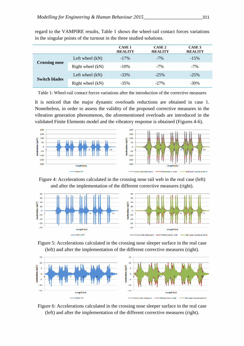
Modelling for Engineering & Human Behaviour 2015________________________311
regard to the VAMPIRE results, Table 1 shows the wheel-rail contact forces variations
in the singular points of the turnout in the three studied solutions.
CASE 1
/REALITY
CASE 2
/REALITY
CASE 3
/REALITY
Crossing nose Left wheel (kN) -17% -7% -15%
Right wheel (kN) -10% -7% -7%
Switch blades Left wheel (kN) -33% -25% -25%
Right wheel (kN) -35% -27% -30%
Table 1: Wheel-rail contact forces variations after the introduction of the corrective measures
It is noticed that the major dynamic overloads reductions are obtained in case 1.
Nonetheless, in order to assess the validity of the proposed corrective measures in the
vibration generation phenomenon, the aforementioned overloads are introduced in the
validated Finite Elements model and the vibratory response is obtained (Figures 4-6).
Figure 4: Accelerations calculated in the crossing nose rail web in the real case (left)
and after the implementation of the different corrective measures (right).
Figure 5: Accelerations calculated in the crossing nose sleeper surface in the real case
(left) and after the implementation of the different corrective measures (right).
Figure 6: Accelerations calculated in the crossing nose sleeper surface in the real case
(left) and after the implementation of the different corrective measures (right).
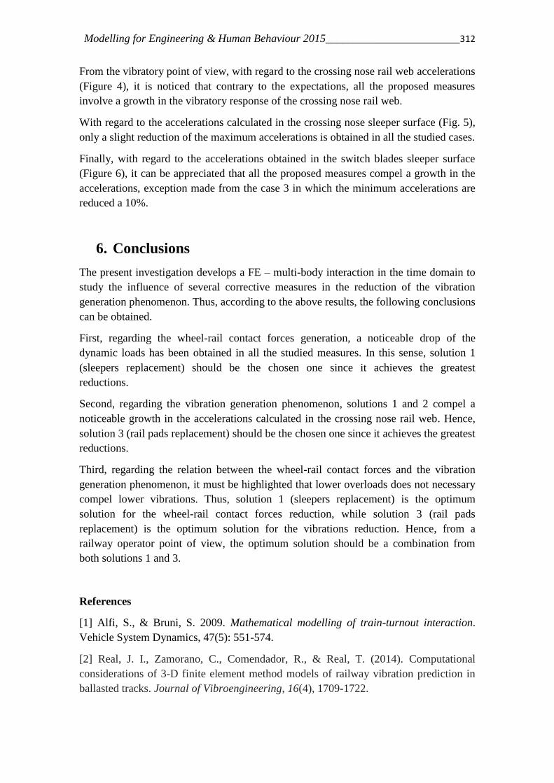
Modelling for Engineering & Human Behaviour 2015________________________312
From the vibratory point of view, with regard to the crossing nose rail web accelerations
(Figure 4), it is noticed that contrary to the expectations, all the proposed measures
involve a growth in the vibratory response of the crossing nose rail web.
With regard to the accelerations calculated in the crossing nose sleeper surface (Fig. 5),
only a slight reduction of the maximum accelerations is obtained in all the studied cases.
Finally, with regard to the accelerations obtained in the switch blades sleeper surface
(Figure 6), it can be appreciated that all the proposed measures compel a growth in the
accelerations, exception made from the case 3 in which the minimum accelerations are
reduced a 10%.
6. Conclusions
The present investigation develops a FE – multi-body interaction in the time domain to
study the influence of several corrective measures in the reduction of the vibration
generation phenomenon. Thus, according to the above results, the following conclusions
can be obtained.
First, regarding the wheel-rail contact forces generation, a noticeable drop of the
dynamic loads has been obtained in all the studied measures. In this sense, solution 1
(sleepers replacement) should be the chosen one since it achieves the greatest
reductions.
Second, regarding the vibration generation phenomenon, solutions 1 and 2 compel a
noticeable growth in the accelerations calculated in the crossing nose rail web. Hence,
solution 3 (rail pads replacement) should be the chosen one since it achieves the greatest
reductions.
Third, regarding the relation between the wheel-rail contact forces and the vibration
generation phenomenon, it must be highlighted that lower overloads does not necessary
compel lower vibrations. Thus, solution 1 (sleepers replacement) is the optimum
solution for the wheel-rail contact forces reduction, while solution 3 (rail pads
replacement) is the optimum solution for the vibrations reduction. Hence, from a
railway operator point of view, the optimum solution should be a combination from
both solutions 1 and 3.
References
[1] Alfi, S., & Bruni, S. 2009. Mathematical modelling of train-turnout interaction.
Vehicle System Dynamics, 47(5): 551-574.
[2] Real, J. I., Zamorano, C., Comendador, R., & Real, T. (2014). Computational
considerations of 3-D finite element method models of railway vibration prediction in
ballasted tracks. Journal of Vibroengineering, 16(4), 1709-1722.

Modelling for Engineering & Human Behaviour 2015________________________313
Assessment of train derailment risk in ballasted an slab tracks with failed fasteners
S. Morales1, J.I. Real
2, L. Montalbán
3, T. Real
4
1, 2,3,4 University Institute for Multidisciplinary Mathematics, Polytechnic University of
Valencia, 14 Camino de Vera, 46022 Valencia, Spain 1Corresponding author. (Tel. +34 963877000; Fax. +34 963877371
E-mail: [email protected],
1. Introduction
It is well known that curved layouts have a great influence on the dynamic behavior of
the vehicle-track system. Thus, correct designs as well as an effective maintenance plan
are key aspects to prevent and correct the deterioration of the vehicle and the track.
Vehicle-track dynamics in curves are closely related to derailments [1]. For this reason,
in [2] track and vehicle conditions are related with the proclivity to derailment in curves
of small radii. This study revealed that the derailment coefficient decreases as the curve
radius increases. Another similar research was conducted in [3] using the simulation
software SIMPACK. A deeper analysis about the influence of the curve parameters and
vehicle speed on derailment was presented in [4], employing the commercial software
ADAMS/Rail. Derailment in a high-radius curve (7000 m) including the effect of the
fastener failure is analyzed in [5]; this study demonstrated that in this high-radius
concrete curve, the stability of a high speed train is not compromised if the number of
failed fasteners is lower than 15.
The relationship between flawed fasteners and derailment risk has been also studied in
[6] in a tangent track using a coupled vehicle/track model. The results show the strong
influence of the disabled fasteners on the derailment coefficient and on the track
widening, which also increases the derailment risk. The research [7], conducted in slab
tracks, concludes that failed fasteners cause increased displacements on the rail and the
slab which become greater with increasing vehicle speed. In [8], the derailment risk in
a curved track is assessed considering failures in the track supports, demonstrating their
great influence on the running safety; the vehicle and the track infrastructure are
modeled as a multi-body system while the rails are modeled as Timoshenko beams
resting on discrete supports. The importance of the lateral dynamics on vehicle stability
has prompted the development of innovative elements, such as frictional sleepers [9] to
increase the lateral resistance of railway tracks, and of new monitoring techniques to
maintain the fasteners in perfect condition [10].
In this context, the present study aims to evaluate the dynamic behavior of the vehicle in
curved tracks where fasteners have failed. However, two different vehicles have been
considered (passengers and freight), with their respective speeds, and two curves of
different radii. Furthermore, all these situations have been evaluated and then compared
in two different scenarios: a ballasted track and a concrete slab track.

Modelling for Engineering & Human Behaviour 2015________________________314
2. Model of the studied track
To assess the risk of derailment, two models have been developed: a track FEM model
and a track-vehicle model.
The FEM model is used to calculate the values of track vertical and lateral stiffness in
different scenarios in which fasteners fail. For this reason, it has been developed to
represent in detail the upper part of the track superstructure, including the rails, the
fasteners and the sleepers which rest on elastic supports that simulate the granular
layers.
Track geometry has been implemented as a mesh of hexahedral elements with a
maximum side of 0.04m. The fastener clip has been represented in detail and the screw
effect has been represented by compressive forces acting on each clip. The lateral and
plan view of the fastener is imported in a CAD file to construct the model in ANSYS.
Regarding the boundary conditions, the length of the model is 9m, long enough to avoid
the influence of the extreme boundaries on the static results, which are always
calculated in the center of the model. Rotations and longitudinal movements of the rail
extremes are constrained in the model boundaries, while the sleeper displacements are
conditioned by spring elements that account for the elastic support.
Once the track model is developed, its stiffness is calibrated with data recorded in a
gathering campaign carried out in a real stretch.
Meanwhile, track-vehicle interaction has been analyzed by means of a multi-body
model performed in the commercial software VAMPIRE Pro. In this model two
vehicles (a passengers and a freight train) have been represented as dynamic systems of
three masses (unsprung, semi-sprung and sprung) connected by spring-damper elements
that simulate the contact with the rail and the vehicle suspensions.
The procedure followed to calculate the risk of derailment in each case is as follows:
First of all, in the track model, fasteners are steadily removed to calculate the variations
produced on the vertical stiffness kv and on the lateral stiffness kh when the fasteners
fail.
Subsequently, vertical and lateral track stiffness values are introduced into the track-
vehicle model, the passage of a vehicle is simulated and the wheel-rail contact forces
calculated. Once these forces are known, derailment coefficient can be finally obtained
as the relationship between lateral and vertical forces in the contact.
3. Simulation of different scenarios
In the present study different scenarios have been presented and their influence on the
risk of derailment has been assessed. Among the studied cases, in first term, the
influence of the number of failed fasteners has been evaluated; then, the importance of
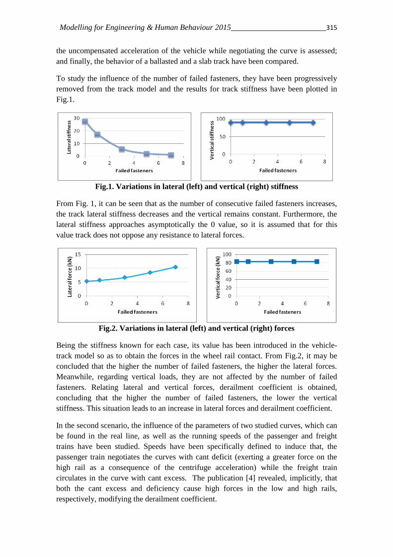
Modelling for Engineering & Human Behaviour 2015________________________315
the uncompensated acceleration of the vehicle while negotiating the curve is assessed;
and finally, the behavior of a ballasted and a slab track have been compared.
To study the influence of the number of failed fasteners, they have been progressively
removed from the track model and the results for track stiffness have been plotted in
Fig.1.
Fig.1. Variations in lateral (left) and vertical (right) stiffness
From Fig. 1, it can be seen that as the number of consecutive failed fasteners increases,
the track lateral stiffness decreases and the vertical remains constant. Furthermore, the
lateral stiffness approaches asymptotically the 0 value, so it is assumed that for this
value track does not oppose any resistance to lateral forces.
Fig.2. Variations in lateral (left) and vertical (right) forces
Being the stiffness known for each case, its value has been introduced in the vehicle-
track model so as to obtain the forces in the wheel rail contact. From Fig.2, it may be
concluded that the higher the number of failed fasteners, the higher the lateral forces.
Meanwhile, regarding vertical loads, they are not affected by the number of failed
fasteners. Relating lateral and vertical forces, derailment coefficient is obtained,
concluding that the higher the number of failed fasteners, the lower the vertical
stiffness. This situation leads to an increase in lateral forces and derailment coefficient.
In the second scenario, the influence of the parameters of two studied curves, which can
be found in the real line, as well as the running speeds of the passenger and freight
trains have been studied. Speeds have been specifically defined to induce that, the
passenger train negotiates the curves with cant deficit (exerting a greater force on the
high rail as a consequence of the centrifuge acceleration) while the freight train
circulates in the curve with cant excess. The publication [4] revealed, implicitly, that
both the cant excess and deficiency cause high forces in the low and high rails,
respectively, modifying the derailment coefficient.
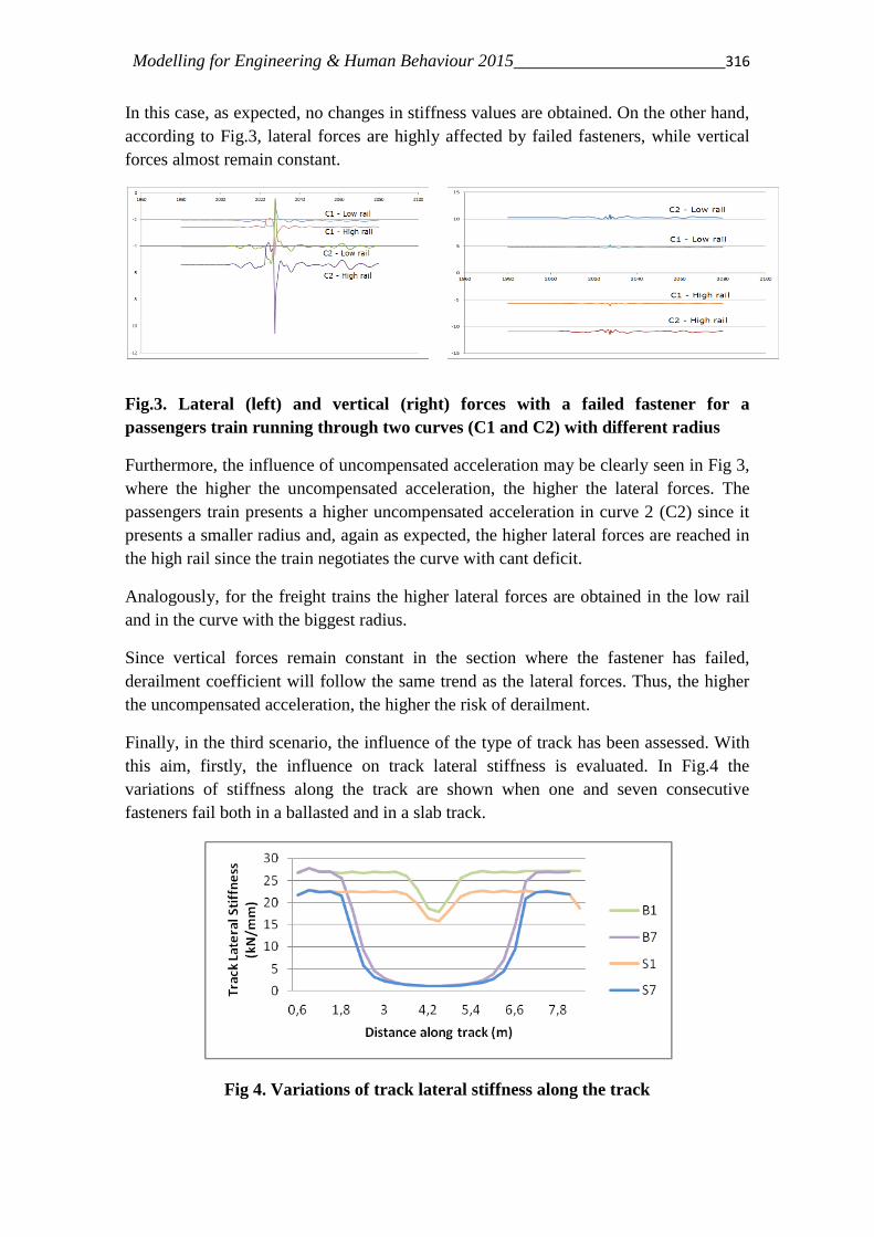
Modelling for Engineering & Human Behaviour 2015________________________316
In this case, as expected, no changes in stiffness values are obtained. On the other hand,
according to Fig.3, lateral forces are highly affected by failed fasteners, while vertical
forces almost remain constant.
Fig.3. Lateral (left) and vertical (right) forces with a failed fastener for a
passengers train running through two curves (C1 and C2) with different radius
Furthermore, the influence of uncompensated acceleration may be clearly seen in Fig 3,
where the higher the uncompensated acceleration, the higher the lateral forces. The
passengers train presents a higher uncompensated acceleration in curve 2 (C2) since it
presents a smaller radius and, again as expected, the higher lateral forces are reached in
the high rail since the train negotiates the curve with cant deficit.
Analogously, for the freight trains the higher lateral forces are obtained in the low rail
and in the curve with the biggest radius.
Since vertical forces remain constant in the section where the fastener has failed,
derailment coefficient will follow the same trend as the lateral forces. Thus, the higher
the uncompensated acceleration, the higher the risk of derailment.
Finally, in the third scenario, the influence of the type of track has been assessed. With
this aim, firstly, the influence on track lateral stiffness is evaluated. In Fig.4 the
variations of stiffness along the track are shown when one and seven consecutive
fasteners fail both in a ballasted and in a slab track.
Fig 4. Variations of track lateral stiffness along the track
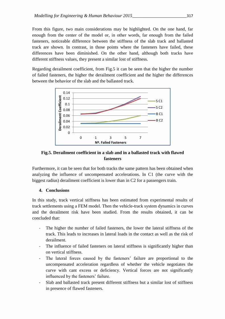
Modelling for Engineering & Human Behaviour 2015________________________317
From this figure, two main considerations may be highlighted. On the one hand, far
enough from the center of the model or, in other words, far enough from the failed
fasteners, noticeable difference between the stiffness of the slab track and ballasted
track are shown. In contrast, in those points where the fasteners have failed, these
differences have been diminished. On the other hand, although both tracks have
different stiffness values, they present a similar lost of stiffness.
Regarding derailment coefficient, from Fig.5 it can be seen that the higher the number
of failed fasteners, the higher the derailment coefficient and the higher the differences
between the behavior of the slab and the ballasted track.
Fig.5. Derailment coefficient in a slab and in a ballasted track with flawed
fasteners
Furthermore, it can be seen that for both tracks the same pattern has been obtained when
analyzing the influence of uncompensated accelerations. In C1 (the curve with the
biggest radius) derailment coefficient is lower than in C2 for a passengers train.
4. Conclusions
In this study, track vertical stiffness has been estimated from experimental results of
track settlements using a FEM model. Then the vehicle-track system dynamics in curves
and the derailment risk have been studied. From the results obtained, it can be
concluded that:
- The higher the number of failed fasteners, the lower the lateral stiffness of the
track. This leads to increases in lateral loads in the contact as well as the risk of
derailment.
- The influence of failed fasteners on lateral stiffness is significantly higher than
on vertical stiffness.
- The lateral forces caused by the fasteners’ failure are proportional to the
uncompensated acceleration regardless of whether the vehicle negotiates the
curve with cant excess or deficiency. Vertical forces are not significantly
influenced by the fasteners’ failure.
- Slab and ballasted track present different stiffness but a similar lost of stiffness
in presence of flawed fasteners.
0
0.02
0.04
0.06
0.08
0.1
0.12
0.14
0 1 3 5 7
De
railm
en
t C
oe
ffic
ien
t
Nº. Failed Fasteners
S C1
S C2
B C1
B C2
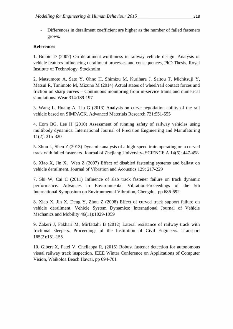
Modelling for Engineering & Human Behaviour 2015________________________318
- Differences in derailment coefficient are higher as the number of failed fasteners
grows.
References
1. Brabie D (2007) On derailment-worthiness in railway vehicle design. Analysis of
vehicle features influencing derailment processes and consequences, PhD Thesis, Royal
Institute of Technology, Stockholm
2. Matsumoto A, Sato Y, Ohno H, Shimizu M, Kurihara J, Saitou T, Michitsuji Y,
Matsui R, Tanimoto M, Mizuno M (2014) Actual states of wheel/rail contact forces and
friction on sharp curves – Continuous monitoring from in-service trains and numerical
simulations. Wear 314:189-197
3. Wang L, Huang A, Liu G (2013) Analysis on curve negotiation ability of the rail
vehicle based on SIMPACK. Advanced Materials Research 721:551-555
4. Eom BG, Lee H (2010) Assessment of running safety of railway vehicles using
multibody dynamics. International Journal of Precision Engineering and Manufaturing
11(2): 315-320
5. Zhou L, Shen Z (2013) Dynamic analysis of a high-speed train operating on a curved
track with failed fasteners. Journal of Zhejiang University- SCIENCE A 14(6): 447-458
6. Xiao X, Jin X, Wen Z (2007) Effect of disabled fastening systems and ballast on
vehicle derailment. Journal of Vibration and Acoustics 129: 217-229
7. Shi W, Cai C (2011) Influence of slab track fastener failure on track dynamic
performance. Advances in Environmental Vibration-Proceedings of the 5th
International Symposium on Environmental Vibration, Chengdu, pp 686-692
8. Xiao X, Jin X, Deng Y, Zhou Z (2008) Effect of curved track support failure on
vehicle derailment. Vehicle System Dynamics: International Journal of Vehicle
Mechanics and Mobility 46(11):1029-1059
9. Zakeri J, Fakhari M, Mirfattahi B (2012) Lateral resistance of railway track with
frictional sleepers. Proceedings of the Institution of Civil Engineers. Transport
165(2):151-155
10. Gibert X, Patel V, Chellappa R, (2015) Robust fastener detection for autonomous
visual railway track inspection. IEEE Winter Conference on Applications of Computer
Vision, Waikoloa Beach Hawai, pp 694-701
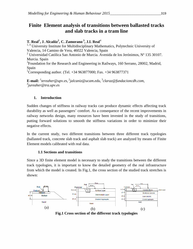
Modelling for Engineering & Human Behaviour 2015___________________________319
Finite Element analysis of transitions between ballasted tracks
and slab tracks in a tram line
T. Real
1, J. Alcañiz
2, C. Zamorano
3, J.I. Real
4
1, 4 University Institute for Multidisciplinary Mathematics, Polytechnic University of
Valencia, 14 Camino de Vera, 46022 Valencia, Spain 2 Universidad Católica San Antonio de Murcia. Avenida de los Jerónimos, Nº 135 30107.
Murcia. Spain 3Foundation for the Research and Engineering in Railways, 160 Serrano, 28002, Madrid,
Spain 1Corresponding author. (Tel. +34 963877000; Fax. +34 963877371
E-mail: [email protected],
1. Introduction
Sudden changes of stiffness in railway tracks can produce dynamic effects affecting track
durability as well as passengers’ comfort. As a consequence of the recent improvements in
railway networks design, many resources have been invested in the study of transitions,
putting forward solutions to smooth the stiffness variations in order to minimize their
negative effects.
In the current study, two different transitions between three different track typologies
(ballasted track, concrete slab track and asphalt slab track) are analyzed by means of Finite
Element models calibrated with real data.
1.1 Sections and transitions
Since a 3D finite element model is necessary to study the transitions between the different
track typologies, it is important to know the detailed geometry of the real infrastructure
from which the model is created. In Fig.1, the cross section of the studied track stretches is
shown:
(a)
(b)
(c)
Fig.1 Cross section of the different track typologies
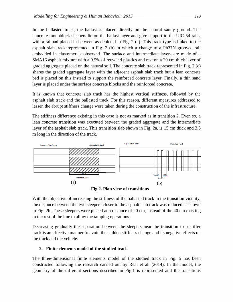
Modelling for Engineering & Human Behaviour 2015___________________________320
In the ballasted track, the ballast is placed directly on the natural sandy ground. The
concrete monoblock sleepers lie on the ballast layer and give support to the UIC-54 rails,
with a railpad placed in between as depicted in Fig. 2 (a). This track type is linked to the
asphalt slab track represented in Fig. 2 (b) in which a change to a Ph37N grooved rail
embedded in elastomer is observed. The surface and intermediate layers are made of a
SMA16 asphalt mixture with a 0.5% of recycled plastics and rest on a 20 cm thick layer of
graded aggregate placed on the natural soil. The concrete slab track represented in Fig. 2 (c)
shares the graded aggregate layer with the adjacent asphalt slab track but a lean concrete
bed is placed on this instead to support the reinforced concrete layer. Finally, a thin sand
layer is placed under the surface concrete blocks and the reinforced concrete.
It is known that concrete slab track has the highest vertical stiffness, followed by the
asphalt slab track and the ballasted track. For this reason, different measures addressed to
lessen the abrupt stiffness change were taken during the construction of the infrastructure.
The stiffness difference existing in this case is not as marked as in transition 2. Even so, a
lean concrete transition was executed between the graded aggregate and the intermediate
layer of the asphalt slab track. This transition slab shown in Fig. 2a, is 15 cm thick and 3.5
m long in the direction of the track.
(a) (b)
Fig.2. Plan view of transitions
With the objective of increasing the stiffness of the ballasted track in the transition vicinity,
the distance between the two sleepers closer to the asphalt slab track was reduced as shown
in Fig. 2b. These sleepers were placed at a distance of 20 cm, instead of the 40 cm existing
in the rest of the line to allow the tamping operations.
Decreasing gradually the separation between the sleepers near the transition to a stiffer
track is an effective manner to avoid the sudden stiffness change and its negative effects on
the track and the vehicle.
2. Finite elements model of the studied track
The three-dimensional finite elements model of the studied track in Fig. 5 has been
constructed following the research carried out by Real et al. (2014). In the model, the
geometry of the different sections described in Fig.1 is represented and the transitions

Modelling for Engineering & Human Behaviour 2015___________________________321
shown in Fig.2 have been implemented as well. The total length of the model is 60m,
divided in 3 stretches of the same length correspondent to each track typology. Two
different analyses are run on this model: one dynamic to obtain the accelerations induced
by the train loads passage and another static to calculate the deflections caused by these
loads and, subsequently, the vertical track stiffness.
The considered load corresponds to that transmitted by the considered vehicle, carrying 4
passengers per square meter in each of the three carriages. The final load result (90
kN/axle) has been incremented to include the dynamic overloads according to the German
criterion explained in Fastenrath (1981). The final load is 63.95 kN/wheel considering
medium track conditions and high statistical precision (95.5%). Vehicle speed has been set
in 35 km/h since all the real registers were measured when the trains run at speeds of 33-36
km/h.
3. Evaluation of improvements for the transition design
Since the most important property that the transition must fulfill is to provide a progressive
variation of the track vertical stiffness, three different methods existing in the literature to
achieve this aim are compared. To do so, from the FEM model, both the static (stiffness)
and dynamic (acceleration) responses are calculated on the track in the different scenarios
considered.
In the first case, a change of the stiffness of the elastomer is proposed, since authors as Lei
and Hang (2011) stated that elastomers have a noticeable influence on the vertical stiffness
of the track. Thus, a more elastic elastomer is chosen for the concrete slab track while the
stiffness elastomers placed over the sleepers on the ballasted track is progressively
increased, being it higher in those sections adjacent to the asphalt slab track. The result of
these changes is plotted in Fig. 3 (stiffness) and Fig. 4 (accelerations).
(a)
(b)
Fig.3. Evolution of the track vertical stiffness at transition 1 (a) and at transition 2 (b)
in the original case (red) and the new scenario (blue)
0
50
100
150
200
250
300
10 20 30Ve
rtic
al S
tiff
ne
ss (
kN/m
m)
Distance (m)
0
50
100
150
200
30 40 50Ve
rtic
al S
tiff
ne
ss (
kN/m
m)
Distance (m)
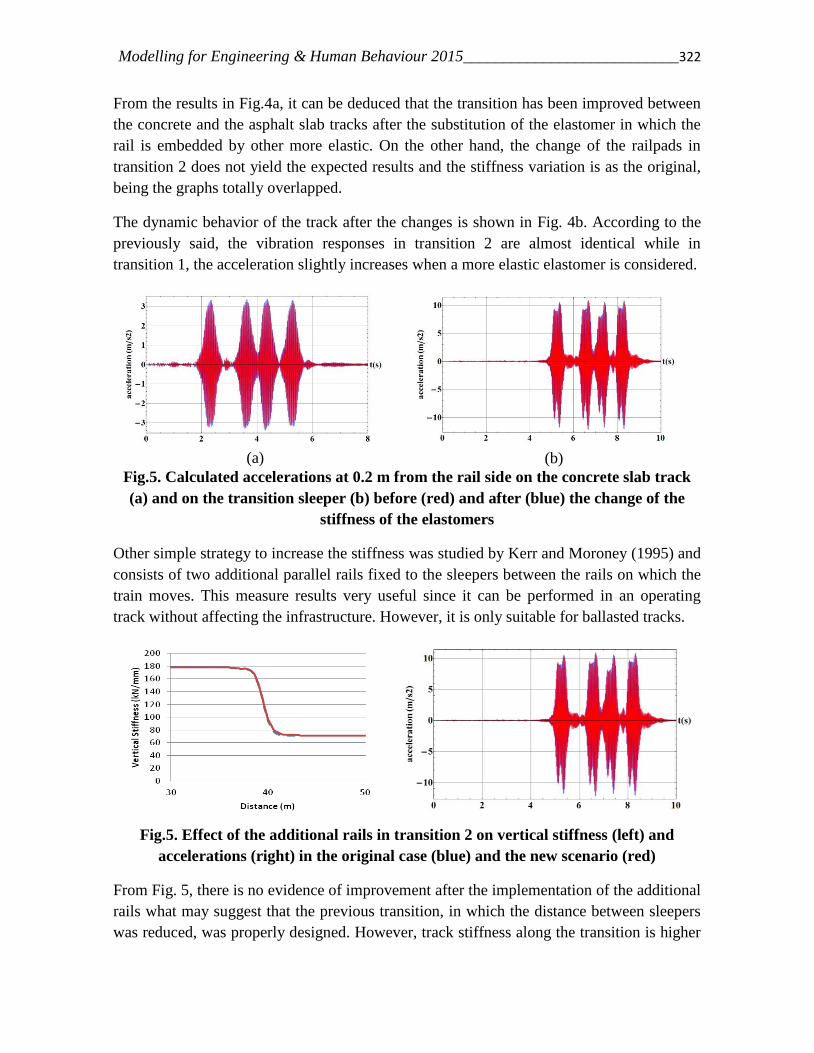
Modelling for Engineering & Human Behaviour 2015___________________________322
From the results in Fig.4a, it can be deduced that the transition has been improved between
the concrete and the asphalt slab tracks after the substitution of the elastomer in which the
rail is embedded by other more elastic. On the other hand, the change of the railpads in
transition 2 does not yield the expected results and the stiffness variation is as the original,
being the graphs totally overlapped.
The dynamic behavior of the track after the changes is shown in Fig. 4b. According to the
previously said, the vibration responses in transition 2 are almost identical while in
transition 1, the acceleration slightly increases when a more elastic elastomer is considered.
(a)
(b)
Fig.5. Calculated accelerations at 0.2 m from the rail side on the concrete slab track
(a) and on the transition sleeper (b) before (red) and after (blue) the change of the
stiffness of the elastomers
Other simple strategy to increase the stiffness was studied by Kerr and Moroney (1995) and
consists of two additional parallel rails fixed to the sleepers between the rails on which the
train moves. This measure results very useful since it can be performed in an operating
track without affecting the infrastructure. However, it is only suitable for ballasted tracks.
Fig.5. Effect of the additional rails in transition 2 on vertical stiffness (left) and
accelerations (right) in the original case (blue) and the new scenario (red)
From Fig. 5, there is no evidence of improvement after the implementation of the additional
rails what may suggest that the previous transition, in which the distance between sleepers
was reduced, was properly designed. However, track stiffness along the transition is higher
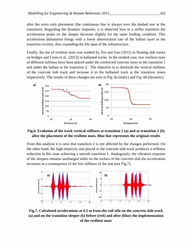
Modelling for Engineering & Human Behaviour 2015___________________________323
after the extra rails placement (the continuous line is always over the dashed one at the
transition). Regarding the dynamic response, it is observed how in a stiffer transition the
acceleration peaks on the sleeper decrease slightly for the same loading condition. This
acceleration diminution brings with a lower deterioration rate of the ballast layer in the
transition vicinity, thus expanding the life span of the infrastructure.
Finally, the use of resilient mats was studied by Xin and Gao (2011) in floating slab tracks
on bridges and Costa et al., (2012) in ballasted tracks. In the studied case, two resilient mats
of different stiffness have been placed under the reinforced concrete layer in the transition 1
and under the ballast in the transition 2. The objective is to diminish the vertical stiffness
of the concrete slab track and increase it in the ballasted track at the transition zones
respectively. The results of these changes are seen in Fig. 6a (static) and Fig. 6b (dynamic).
Fig.6. Evolution of the track vertical stiffness at transition 1 (a) and at transition 2 (b)
after the placement of the resilient mats. Blue line represents the original results
From this analysis it is seen that transition 2 is not affected by the changes performed. On
the other hand, the high-elasticity mat placed in the concrete slab track produces a stiffness
reduction in this zone achieving a smooth transition 1. Analogously, the vibration response
of the sleepers remains unchanged while on the surface of the concrete slab the acceleration
increases as a consequence of the low stiffness of the mat (see Fig.7).
Fig.7. Calculated accelerations at 0.2 m from the rail side on the concrete slab track
(a) and on the transition sleeper (b) before (red) and after (blue) the implementation
of the resilient mats
a) b)
a) b)
Modelling for Engineering & Human Behaviour 2015___________________________324
CONCLUSIONS
Two different transitions have been analyzed in this study. These transitions were located
between three different track typologies: ballasted track; asphalt slab track and concrete
slab track. To perform the analysis, a three-dimensional finite elements model has been
developed and validated with real acceleration measurements. From this model, different
scenarios have been assessed. The results of the study revealed:
The stiffness slope in the transition zone between a concrete and an asphalt slab
track can be improved either reducing the elastomer stiffness in the concrete slab
track or using resilient mats under the concrete slab track.
Additional rails on the ballasted track do not contribute achieve a smoother
transition. The sole reduction of the sleeper spacing in the sleepers closer to the
transition is recommended instead.
Neither the elastomer stiffness nor the resilient mats have improved the transition
behavior between asphalt and concrete slab tracks. In the cases in which the
stiffness slope is too acute, it would be convenient to increase the length of the
transition slab located beneath the asphalt slab track.
The dynamic behavior of the infrastructure is slightly modified when an elastic resilient
mat is placed under the concrete slab track, being the accelerations increased. Otherwise, no
significant changes have been reached.
REFERENCES
Costa, P. A., Calçada, R., & Cardoso, A. (2012). Ballast mats for the reduction of railway
traffic vibrations. Numerical study. Soil Dynamics and Earthquake Engineering , 42, 137-
150.
Fastenrath, F. (1981). Railroad Track: theory and practice: material properties, cross
sections, welding and treatment (1 ed.). New York: F. Ungar Pub. Co.
Kerr, A., & Moroney, B. (1995). Track transition problems and remedies. American
Railway Engineering Association , 742, 267-297.
Lei, X., & Zhang, B. (2011). Analysis of dynamic behavior for slab track of high-speed
railway based on vehicle and track elements. Journal of Transportation Engineering , 137,
227-240.
Real, J., Zamorano, C., Hernández, C., Comendador, R., & Real, T. (2014). Computational
considerations of 3-D finite element method models of railway vibration prediction in
ballasted tracks. Journal of Vibroengineering , 16 (4), 1709-1722.
Xin T., G. L. (2011). Reducing slab track vibration into bridge using elastic materials in
high speed railway. Journal of Sound and Vibration , 330, 2237-2248.
Modelling for Engineering & Human Behaviour_____________________________325
Comparison between analytical and numerical models to predict vibrations in
railway tunnels
Fran Ribes1*, César Hernández
1, Teresa Real
1, Julia Real
1
1Institute for Multidisciplinary Mathematics, Polytechnic University of Valencia,
46022,
Valencia, Spain
*Corresponding author. E-mail: [email protected]
1. INTRODUCTION
The increase of underground railway lines in urban areas has prompted the number of
people affected by railway externalities, such as noise and vibrations. Furthermore,
railway induced vibrations in tunnels may also compromise the stability of the tunnel or
the nearby buildings; for this reason, many mathematical models have been developed
in the last decades to model railway vibrations in the tunnel vicinity.
These mathematical models can be divided in two main groups: two-dimensional (2-D)
and three-dimensional (3-D). As 2-D models only consider wave propagation in the
plane which is perpendicular to the tunnel axis and underestimate soil damping, Gupta
et al. (2007) assert that this approach is not suitable to predict train induced vibrations.
This opinion is also supported by Andersen and Jones (2006), who compared the results
of 2-D and 3-D models, stating that 2-D models can be used to assess vibrations
qualitatively as a consequence of their low computational cost, but that do not yield
precise results.
Simultaneously, vibration prediction models can also be classified in two groups:
analytical and numerical models. Analytical models compute rapidly the exact solution
solving complex differential equations which, in order to be solved, require many
simplifications. The best-extended model available in the current literature is the Pipe-
in-Pipe model, developed by Forrest and Hunt (2006) and subsequently completed by
Hussein and Hunt (2007), Jones and Hunt (2011) and Kuo et al. (2011).
On the contrary, numerical vibration models in tunnels apply the Finite Element Method
(FEM), the Boundary Element Method (BEM) or both together to solve the dynamic
problem. Although numerical models require higher computational effort than analytical
methods, they allow introducing discontinuities and the different elements of the system
in detail.
With the objective of comparing two of the most-extended modeling methodologies in
the literature, the current study computes the vibrations induced by the passage of a
train following two different strategies: the analytical method Pipe-in-Pipe and a
numerical model constructed exclusively using a FEM software.

Modelling for Engineering & Human Behaviour_____________________________326
2. STUDIED SECCTION
The tunnel used in this study has a circular section with an inner diameter of 8.43m. The
tunnel structure is made of reinforced concrete segments, with a thickness of 0.32 cm,
and a 0.18 cm concrete grout. There are two parallel tracks of Iberian gauge (1.668m),
formed by UIC-60 rails embedded in the concrete slab using the system EDILON
Corkelast®.
The soil in which the tunnel is embedded is formed by alternating layers of silty sand
and clayey gravel. The water table is located at a depth equivalent to the tunnel center,
for this reason two different soils have been considered: saturated and non-saturated.
3. NUMERICAL MODEL
The FEM model is solved using the software ANSYS LS-DYNA. The dynamic
problem is expressed by the forced vibration equation where [M] is the global mass
matrix, [C] the damping matrix, [K] de stiffness matrix. In the other side of the
equation, the time dependent forces vector appears.
[𝑀] + [𝐶] + [𝐾]𝒖 = 𝑭𝒂(𝒕) (1)
The damping matrix must be determined in order to solve the dynamical problem. the
damping matrix is determined as a linear combination of the mass matrix [M] and the
stiffness matrix [K].
[𝐶] = 𝛼[𝑀] + 𝛽[𝐾] (2)
Regarding to the structure, the modeling must accurately represent the details and sizes
of the different elements (Fig.1). However, in order to reduce the computational
calculation time and meet the elements dimensions criteria imposed by the software,
some simplifications have been assumed. These simplifications are carefully chosen in
order to avoid any loss of accuracy in the final results.
Fig.1. FEM model of the track-tunnel-soil system
The material behavior is assumed to be linear elastic. This hypothesis is assumed
because it has been previously checked that the moving train does not induce large
strains in the soil in this case.

Modelling for Engineering & Human Behaviour_____________________________327
The vehicle is simulated as a three-mass system where the wheel–rail interaction is
modeled as a node-to-beam contact allowing for sliding and loss of contact, using the
Penalty algorithm. The contact elements provide an elastic support between the rail and
the wheel simulating the hertzian contact.
The full Newton–Raphson method is used to solve the non-linear equations of the
problem. The Newmark implicit time integration method is used, to solve the transient
dynamic equilibrium equations.
In numerical model, the elasticity modulus of the soil is subjected to a calibration
process to represent in the modeled homogeneous soil the same dynamic properties of
the real stratified soil. The different accelerograms obtained from the different values
chosen are compared with real accelerations registers measured in a point located at the
tunnel support.
Numerical model has been calibrated in time domain, but in order to compare it with the
numerical models results the frequency domain results have to be also in accordance
with measured results.
4. ANALYTICAL MODEL
The main characteristic of the Pipe-in-Pipe model (Forrest and Hunt (2006)) is that
considers the soil as a hollow cylinder of infinite length into which the tunnel is
embedded. Into the tunnel, there is a concrete slab which supports the rails. The
concrete slab and the rails are modeled as Euler-Bernouilli beams subjected to bending
forces. Between the rails and the slab there are railpads which provide an elastic support
for the rail while between the slab and the tunnel invert there is an elastic mat. The
displacements among the different elements in the model are coupled in the frequency
and wavenumber domain, in which the dynamic problem is also solved.
The wave propagation phenomenon through the soil is studied via the wave equation,
considering a solid, homogeneous, isotropic and linear-elastic medium for the tunnel
structure and the soil. The wave equation is displayed in Eq.(3), in which u is the
displacement vector; λ and μ are Lamé constants of the material; ρ is the density of the
material; f the volumetric forces and t is the independent variable time. Although it is a
3-D model, the dynamic behavior in the tunnel direction is assumed to remain
invariable in order to simplify the calculations.
(λ + μ)∇∇ ∙ u + μ∇2u + ρf = ρ∂2u
∂t2 (3)
Eq. (3) is also solved in the frequency and wavenumber domain, obtaining the field of
displacements u produced by a unit load acting in the tunnel invert in the vertical and
horizontal direction (See Hussein and Hunt (2007)). The coupling between the concrete
structure of the tunnel and the natural soil is solved taking into account that the values
of the field of displacements in the tunnel outer surface must be equal to the
Modelling for Engineering & Human Behaviour_____________________________328
displacements in the soil adjacent to the tunnel and that there must exist equilibrium of
external forces in that tunnel-soil interface.
The unit load is introduced as a harmonic excitation along the tunnel axis, taking into
account only the unsprung mass of the vehicle. Moreover, this load is decomposed
using Fourier series along the circular cross section as a summation of sinusoidal terms
in the three space directions (Gupta et al. (2007)). The resulting expression of the unit
load, acting at time t in the position x, in the j-th special direction in wavenumber-
frequency domain is represented in Eq.4, in which 𝑗𝑗𝑛 is the value of the unit load in
frequency-wavenumber domain; n accounts for the term of the Fourier series
decomposition; θ is the angle; ϕ depends on the load direction and ω and ξ are,
respectively, the frequency and the wavenumber.
𝑞𝑗(𝑥, 𝑡) = 𝑗𝑛𝑠𝑖𝑛 (𝑛𝜃 + 𝜙)𝑒𝑗(𝜔𝑡+𝜉𝑥) (4)
After solving the wave equation (3) for the unit load condition, the resulting
displacements for each space direction have an analogous expression, where the term
Ujjn represents the displacement calculated in the frequency-wavenumber domain.
𝑢𝑗(𝑥, 𝑡) = 𝑗𝑛𝑠𝑖𝑛 (𝑛𝜃 + 𝜙)𝑒𝑗(𝜔𝑡+𝜉𝑥) (5)
Hussein and Hunt (2009) implemented the complex model Pipe-in-Pipe in a software
programmed in Matlab. Introducing the vehicle, track, tunnel and soil inputs the
system’s response is directly computed in a specified frequency range.
The aim of this paper is to compare the calculated results from both models in order to
check the strengths of each methodology. For that reason, in analytical model, the same
characteristics as in the numerical model have been considered. However, there are
some differences between the input parameters each model requires. Despite the
majority could to be converted as an equivalent, the damping coefficients used in
numerical models are not available in the “Pipe-in-Pipe” model. Hence loss factor has
been calibrated in order to match the calculated results with the measured registers in
frequency domain.
5. RESULTS
In this section, the results obtained from both models are compared. To do this, the
results from three different points will be obtained. These points are located in the
surrounding soil. Must be noticed that Analytical model do not provide results in the
track elements.
Observing the results (Fig.2) is noticed that the frequency band from 20 to 80 Hz are
relatively close each other. However in the low frequency range there are noticeable
differences.
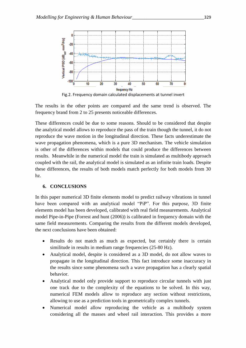
Modelling for Engineering & Human Behaviour_____________________________329
Fig.2. Frequency domain calculated displacements at tunnel invert
The results in the other points are compared and the same trend is observed. The
frequency brand from 2 to 25 presents noticeable differences.
These differences could be due to some reasons. Should to be considered that despite
the analytical model allows to reproduce the pass of the train though the tunnel, it do not
reproduce the wave motion in the longitudinal direction. These facts underestimate the
wave propagation phenomena, which is a pure 3D mechanism. The vehicle simulation
is other of the differences within models that could produce the differences between
results. Meanwhile in the numerical model the train is simulated as multibody approach
coupled with the rail, the analytical model is simulated as an infinite train loads. Despite
these differences, the results of both models match perfectly for both models from 30
hz.
6. CONCLUSIONS
In this paper numerical 3D finite elements model to predict railway vibrations in tunnel
have been compared with an analytical model “PiP”. For this purpose, 3D finite
elements model has been developed, calibrated with real field measurements. Analytical
model Pipe-in-Pipe (Forrest and hunt (2006)) is calibrated in frequency domain with the
same field measurements. Comparing the results from the different models developed,
the next conclusions have been obtained:
Results do not match as much as expected, but certainly there is certain
similitude in results in medium range frequencies (25-80 Hz).
Analytical model, despite is considered as a 3D model, do not allow waves to
propagate in the longitudinal direction. This fact introduce some inaccuracy in
the results since some phenomena such a wave propagation has a clearly spatial
behavior.
Analytical model only provide support to reproduce circular tunnels with just
one track due to the complexity of the equations to be solved. In this way,
numerical FEM models allow to reproduce any section without restrictions,
allowing to use as a prediction tools in geometrically complex tunnels.
Numerical model allow reproducing the vehicle as a multibody system
considering all the masses and wheel rail interaction. This provides a more
Modelling for Engineering & Human Behaviour_____________________________330
accurate reproduction of the train circulating that the infinite train of loads
moving along the tunnel considered in the analytical model
On the other hand, computing time is one of the most important factors when
defining the modeling strategy. In this regard, the simulation of the unbounded
domain as absorbing boundaries and the great amount of elements needed stand
as the major disadvantage of the 3D FEM models. In the studied case,
computing time is around of 20 hours for the FEM model while this time can be
reduced up to 2 minutes in the case of Pipe-in-Pipe model. Therefore, even
though 3D fem model provides a better reproduction of the dynamic response,
the lower calculation time make analytical models interesting tools when there
exist time or computing limitations.
References
Andersen, L, y C.J.C Jones. «Coupled boundary and finite element analysis of vibration from
railway tunnels - a comparison of two- and three-dimensional models.» Journal of Sound and
Vibration, 293 (3-5), 2006: 611-625.
Forrest, J.A, y H.E.M Hunt. «A three-dimensional tunnel model for calculation of train-induced
ground vibration.» Journal of Sound and Vibration 294 (2006): 678-705.
Gupta, S, M.F.M Hussein, G Degrande, H.E.M Hunt, y D. Clouteau. «A comparison of two
numerical models for the prediction of vibrations from underground railway traffic.» Soil
Dynamics and Earthquake Engineering 27 (2007): 608-624.
Hussein, M.F.M, y H.E.M Hunt. «A computationally efficient software application for
calculating vibration from underground railways.» Jounal of Physics: Conference Series 181
(2009): 1-6.
Hussein, M.F.M, y H.E.M Hunt. «A numerical model for calculating vibration from a railway
tunnel embedded in a full-space.» Journal of Sound and Vibration 305 (2007): 401-431.
Kuo, K. A, H.E.M Hunt, y M.F.M Hussein. «The effect of a twin tunnel on the propagation of
ground-borne vibration from an underground railway.» Journal of Sound and Vibration 330
(2011): 6203-6222.
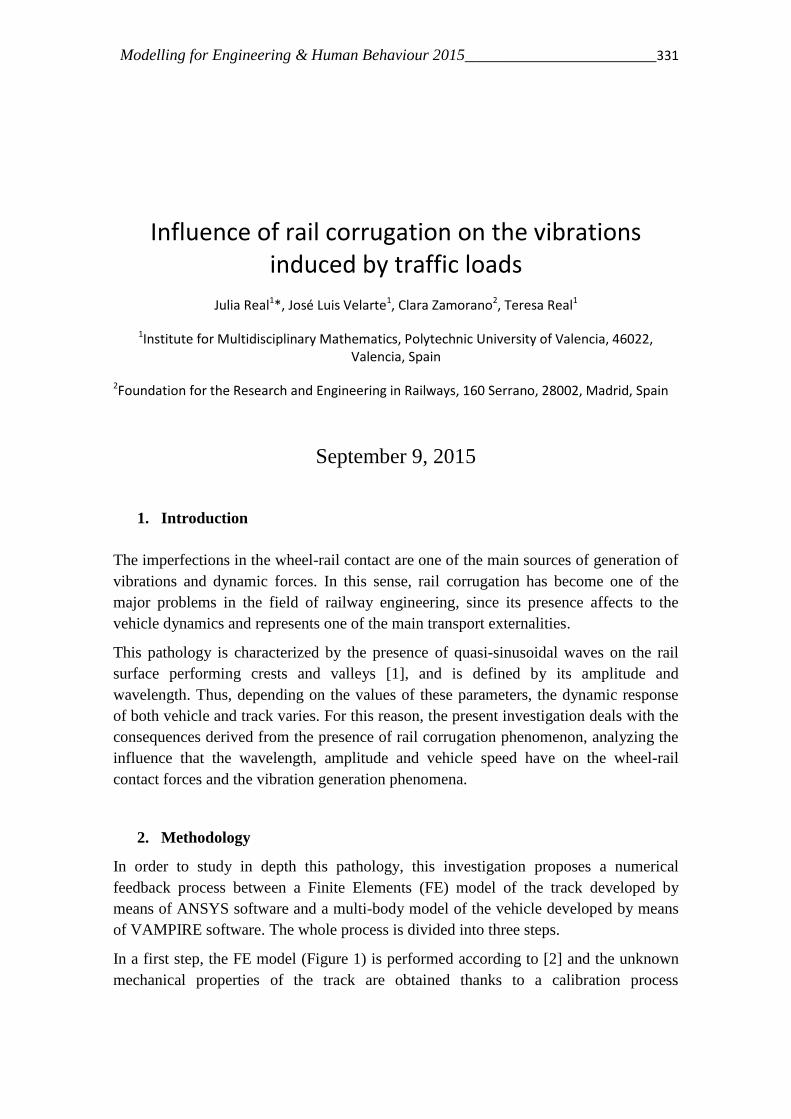
Modelling for Engineering & Human Behaviour 2015________________________331
Influence of rail corrugation on the vibrations induced by traffic loads
Julia Real1*, José Luis Velarte1, Clara Zamorano2, Teresa Real1
1Institute for Multidisciplinary Mathematics, Polytechnic University of Valencia, 46022, Valencia, Spain
2Foundation for the Research and Engineering in Railways, 160 Serrano, 28002, Madrid, Spain
September 9, 2015
1. Introduction
The imperfections in the wheel-rail contact are one of the main sources of generation of
vibrations and dynamic forces. In this sense, rail corrugation has become one of the
major problems in the field of railway engineering, since its presence affects to the
vehicle dynamics and represents one of the main transport externalities.
This pathology is characterized by the presence of quasi-sinusoidal waves on the rail
surface performing crests and valleys [1], and is defined by its amplitude and
wavelength. Thus, depending on the values of these parameters, the dynamic response
of both vehicle and track varies. For this reason, the present investigation deals with the
consequences derived from the presence of rail corrugation phenomenon, analyzing the
influence that the wavelength, amplitude and vehicle speed have on the wheel-rail
contact forces and the vibration generation phenomena.
2. Methodology
In order to study in depth this pathology, this investigation proposes a numerical
feedback process between a Finite Elements (FE) model of the track developed by
means of ANSYS software and a multi-body model of the vehicle developed by means
of VAMPIRE software. The whole process is divided into three steps.
In a first step, the FE model (Figure 1) is performed according to [2] and the unknown
mechanical properties of the track are obtained thanks to a calibration process
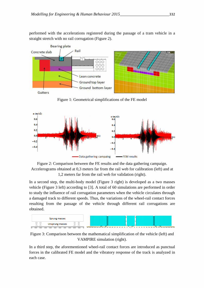
Modelling for Engineering & Human Behaviour 2015________________________332
performed with the accelerations registered during the passage of a tram vehicle in a
straight stretch with no rail corrugation (Figure 2).
Figure 1: Geometrical simplifications of the FE model
Figure 2: Comparison between the FE results and the data gathering campaign.
Accelerograms obtained at 0,3 meters far from the rail web for calibration (left) and at
1,2 meters far from the rail web for validation (right).
In a second step, the multi-body model (Figure 3 right) is developed as a two masses
vehicle (Figure 3 left) according to [3]. A total of 60 simulations are performed in order
to study the influence of rail corrugation parameters when the vehicle circulates through
a damaged track to different speeds. Thus, the variations of the wheel-rail contact forces
resulting from the passage of the vehicle through different rail corrugations are
obtained.
Figure 3: Comparison between the mathematical simplification of the vehicle (left) and
VAMPIRE simulation (right).
In a third step, the aforementioned wheel-rail contact forces are introduced as punctual
forces in the calibrated FE model and the vibratory response of the track is analyzed in
each case.

Modelling for Engineering & Human Behaviour 2015________________________333
The result of the whole process allows obtaining several conclusions about the influence
of rail corrugation parameters on both dynamic forces generation and the vibrations
generation phenomena.
3. Simulations and results
In order to study the influence of rail corrugation on vehicle-track dynamics, a
sensitivity analysis of rail corrugation parameters has been performed according to the
typical values collected in [4]. Thus, a total of 6 combinations have been studied (Table
1) for a speed range from 10 to 100 km/h in steps of 10 km/h (60 simulations).
λ=0.25m λ=0.5m λ=1m
A=0.15mm YES YES YES
A=0.3mm NO YES YES
A=0.5mm NO NO YES
Table 1: Combinations of the rail corrugation parameters
The influence of rail corrugation parameters on the vehicle-track dynamics has been
studied from two different points of view. The first one is focused on the wheel-rail
contact forces generation phenomenon, while the second one is focused on the vibration
generation phenomenon.
With regard to the first one, all the simulations have been performed in VAMPIRE
software. As an example of the results, the following Figure shows a comparison
between the wheel-rail contact forces obtained when a vehicle circulates at two different
speeds (30km/h and 70 km/h) through a track with the presence of a rail corrugation of
A=0.3 mm amplitude and λ=0.5 meters wavelength.
Figure 4: Wheel-rail contact forces generated in a track with the presence of a rail
corrugation of 0.3 mm amplitude and 0.5 meters wavelength when a vehicle circulates
at two different speeds: 30km/h and 70 km/h
It can be appreciated that, in both cases, a heterogeneous pattern takes place.
Nevertheless, the distance between the maximum and minimum peaks matches with the
rail corrugation wavelength (0.5 meters). The main reason of this heterogeneous pattern
is that the wheel-rail contact patch varies as a consequence of the combination between
the rail corrugation geometry and vehicle speed.
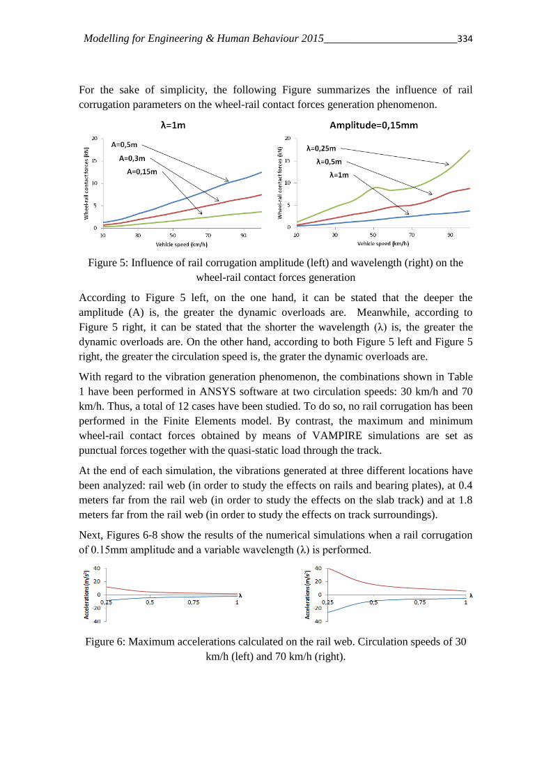
Modelling for Engineering & Human Behaviour 2015________________________334
For the sake of simplicity, the following Figure summarizes the influence of rail
corrugation parameters on the wheel-rail contact forces generation phenomenon.
Figure 5: Influence of rail corrugation amplitude (left) and wavelength (right) on the
wheel-rail contact forces generation
According to Figure 5 left, on the one hand, it can be stated that the deeper the
amplitude (A) is, the greater the dynamic overloads are. Meanwhile, according to
Figure 5 right, it can be stated that the shorter the wavelength (λ) is, the greater the
dynamic overloads are. On the other hand, according to both Figure 5 left and Figure 5
right, the greater the circulation speed is, the grater the dynamic overloads are.
With regard to the vibration generation phenomenon, the combinations shown in Table
1 have been performed in ANSYS software at two circulation speeds: 30 km/h and 70
km/h. Thus, a total of 12 cases have been studied. To do so, no rail corrugation has been
performed in the Finite Elements model. By contrast, the maximum and minimum
wheel-rail contact forces obtained by means of VAMPIRE simulations are set as
punctual forces together with the quasi-static load through the track.
At the end of each simulation, the vibrations generated at three different locations have
been analyzed: rail web (in order to study the effects on rails and bearing plates), at 0.4
meters far from the rail web (in order to study the effects on the slab track) and at 1.8
meters far from the rail web (in order to study the effects on track surroundings).
Next, Figures 6-8 show the results of the numerical simulations when a rail corrugation
of 0.15mm amplitude and a variable wavelength (λ) is performed.
Figure 6: Maximum accelerations calculated on the rail web. Circulation speeds of 30
km/h (left) and 70 km/h (right).

Modelling for Engineering & Human Behaviour 2015________________________335
Figure 7: Maximum accelerations calculated at 0.4 meters far from the rail web.
Circulation speeds of 30 km/h (left) and 70 km/h (right).
Figure 8: Maximum accelerations calculated at 1.8 meters far from the rail web.
Circulation speeds of 30 km/h (left) and 70 km/h (right).
According to Figures 6-8, on the one hand, the shorter the wavelength is, the greater the
accelerations are. On the other hand, the greater the circulation speed is, the greater the
accelerations are. Nevertheless, the effect of circulation speed decreases with the
distance to the track. Thus, the vibrations generated at the rail web (Figure 6) are 16
m/s2
when the vehicle circulates at 30 km/h and 40 m/s2
when the vehicle circulates at
30 km/h (230% higher). Nevertheless, this difference is reduced to 103% in Figure 7
and 14% in Figure 8.
Next, Figures 9-11 show the results of the numerical simulations when a rail
corrugation of λ=1m wavelength and a variable amplitude (A) is performed.
Figure 9: Maximum accelerations calculated on the rail web. Circulation speeds of 30
km/h (left) and 70 km/h (right).
Figure 10: Maximum accelerations calculated at 0.4 meters far from the rail web.
Circulation speeds of 30 km/h (left) and 70 km/h (right).

Modelling for Engineering & Human Behaviour 2015________________________336
Figure 11: Maximum accelerations calculated at 1.8 meters far from the rail web.
Circulation speeds of 30 km/h (left) and 70 km/h (right).
According to Figures 9-11, on the one hand, the deeper the amplitude is, the greater the
dynamic overloads are. On the other hand, as occurred in Figures 6-8, the greater the
circulation speed is, the greater the accelerations are. Meanwhile, the effect of
circulation speed decreases with the distance to the rail web.
4. Conclusions
In this work, a method consisting in a numerical feedback of a FE model of a track and
a multi-body model of a vehicle has been presented in order to study the influence of
rail corrugation parameters and vehicle circulation speed on the dynamic response of a
tram track. Thus, according to the numerical results, it can be stated that the shorter and
the deeper the rail corrugation is, the greater the wheel-rail contact forces and vibrations
are.
In this sense, the vehicle speed is also a key factor. Thus, the greater the circulation
speed is, the greater the dynamic overloads and accelerations are. Nevertheless, its
influence decreases with the distance to the rails.
REFERENCES
[1] Grassie, S. L. (2009). Rail corrugation: characteristics, causes, and
treatments. Proceedings of the Institution of Mechanical Engineers, Part F: Journal of
Rail and Rapid Transit, 223(6), 581-596.
[2] Real, J. I., Zamorano, C., Comendador, R., & Real, T. (2014). Computational
considerations of 3-D finite element method models of railway vibration prediction in
ballasted tracks. Journal of Vibroengineering, 16(4), 1709-1722.
[3] Real, J. I., Zamorano, C., Velarte, J. L., & Blanco, A. E. (2015). Development of a
vehicle–track interaction model to predict the vibratory benefits of rail grinding in the
time domain. Journal of Modern Transportation, 23(3), 189-201.
[4] Spanish regulations N.R.V. 7-5-2.1. (1993). Conservación de la vía. Amolado de las
superficies activas del carril, en vía. RENFE, Dirección de Mantenimiento de
Infraestructura.
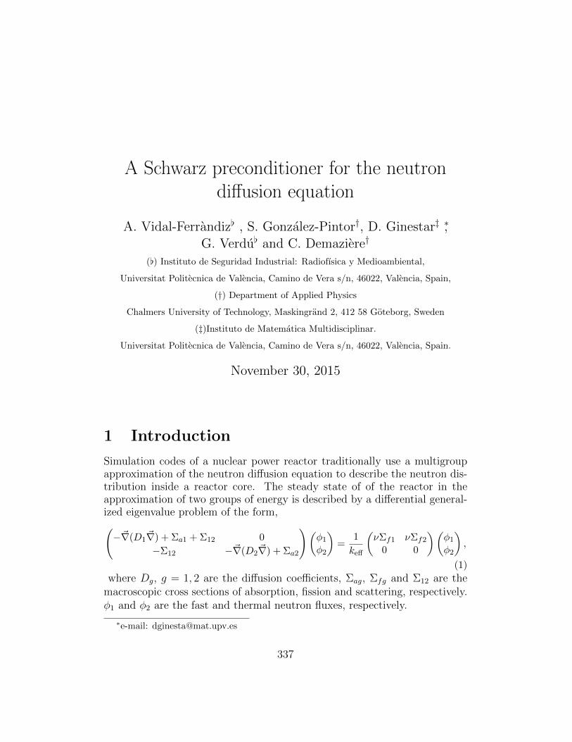
A Schwarz preconditioner for the neutrondiffusion equation
A. Vidal-Ferrandiz[ , S. Gonzalez-Pintor†, D. Ginestar‡ ∗,
G. Verdu[ and C. Demaziere†
([) Instituto de Seguridad Industrial: Radiofısica y Medioambiental,
Universitat Politecnica de Valencia, Camino de Vera s/n, 46022, Valencia, Spain,
(†) Department of Applied Physics
Chalmers University of Technology, Maskingrand 2, 412 58 Goteborg, Sweden
(‡)Instituto de Matematica Multidisciplinar.
Universitat Politecnica de Valencia, Camino de Vera s/n, 46022, Valencia, Spain.
November 30, 2015
1 Introduction
Simulation codes of a nuclear power reactor traditionally use a multigroupapproximation of the neutron diffusion equation to describe the neutron dis-tribution inside a reactor core. The steady state of of the reactor in theapproximation of two groups of energy is described by a differential general-ized eigenvalue problem of the form,(−~∇(D1
~∇) + Σa1 + Σ12 0
−Σ12 −~∇(D2~∇) + Σa2
)(φ1
φ2
)=
1
keff
(νΣf1 νΣf2
0 0
)(φ1
φ2
),
(1)
where Dg, g = 1, 2 are the diffusion coefficients, Σag, Σfg and Σ12 are themacroscopic cross sections of absorption, fission and scattering, respectively.φ1 and φ2 are the fast and thermal neutron fluxes, respectively.
∗e-mail: [email protected]
337
Modelling for Engineering & Human Behaviour 2015 338
Once a spatial discretization has been selected, the problem is reduced toits corresponding algebraic set of equations. To solve the algebraic eigenvalueproblem it is necessary to solve linear systems associated with t block ma-trices, corresponding tot the energy groups. These systems are solved usinga preconditioned Krylov method. For the spatial discretization of equation(1) a high order Finite Element Method (FEM) is used [1], which makesuse of Lagrange polynomials whose nodes form a Gauss-Lobbato quadratureset. These polynomials provide a partition of the shape functions into ver-tices, edges, faces and interior functions. Using this natural partition thelinear systems of equations associated with each energy group can be solvedusing a Schur Complement method that algebraically decouples the inte-rior degrees of freedom from the other ones. This method is advantageouswhen a high polynomial degree, p, is used in the FEM discretization. Toprecondition the resulting Schur complement system two different strategiesare described. First a substructuring block Jacobi preconditioner is stud-ied where the coupling between the different elements is neglected. Also, adomain decomposition algorithm with overlapping between subdomains, likethe additive Schwarz method, is considered. The performance of the differ-ent approaches is studied numerically using a three-dimensional model of areactor core.
2 Schur complement method
Consider the solution of a generic linear system,
Ax = f , (2)
which can be structured as,(Abb Abi
ATbi Aii
)(xbxi
)=
(fbfi
), (3)
where the degrees of freedom related to the interior of the finite elements aredecoupled algebraically using a technique known as the Schur complementmethod. This manipulation decomposes the system into the contributionsrelated to the subdomain boundaries, b, union of the vertices, edges and facesshape functions; and the interior shape functions, i. The resulting system isof the same size as of the boundary degrees of freedom and is written as,
Sxb = fS , (4)
Modelling for Engineering & Human Behaviour 2015 339
S = Abb − AbiA−1ii A
Tbi , fS = fb − AbiA
−1ii fi , and xi = A−1
ii (fi − ATbixb) .
2.1 Subtructuring preconditioner
In the same way as the original matrix, the Schur complement matrix has anstructure that can be algebraically separated into vertices, edges and facesdegrees of freedom, as followsSvv Sve Svf
STve See Sef
STvf ST
ef Sff
xb,vxb,exb,f
=
fS,vfS,efS,f
. (5)
A substructuring preconditioner for this system can be defined as,
Pvef =
Svv 0 00 block-diag(See) 00 0 block-diag(Sff )
−1
. (6)
The submatrices See and Sff represent the whole set of edges and facesdegrees of freedom, respectively. However, in the proposed preconditioner,each edge and each face is considered independently neglecting the interac-tions between different edges or faces forcing a block diagonal structure forthe submatrices.
For comparative reasons a simple diagonal Jacobi preconditioner, Pd, anda classical incomplete LU decomposition, PILU , are also implemented.
2.2 Restricted Additive Schwarz
Another possibility of preconditioning consists of introducing and overlappingbetween the subdomains by including the degrees of related to the verticesand edges in the different blocks. The last preconditioner is referred as aRestricted Additive Schwarz (RAS),
PRAS =K∑k
RTkXk (RkSRk)−1Rk, (7)
where the subdomain k is the complete union of two finite element cells, Rk
denote the restriction operator from the global domain to the subdomain k,RT
k in the corresponding extension operator and Xk is a partition of unitymatrix that scales the contribution of each degrees of freedom depending thenumber subdomain of in which it is present.
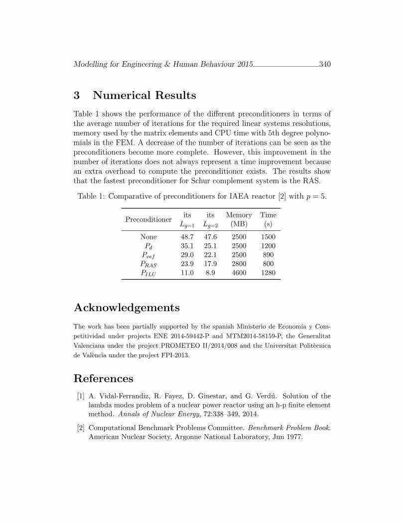
Modelling for Engineering & Human Behaviour 2015 340
3 Numerical Results
Table 1 shows the performance of the different preconditioners in terms ofthe average number of iterations for the required linear systems resolutions,memory used by the matrix elements and CPU time with 5th degree polyno-mials in the FEM. A decrease of the number of iterations can be seen as thepreconditioners become more complete. However, this improvement in thenumber of iterations does not always represent a time improvement becausean extra overhead to compute the preconditioner exists. The results showthat the fastest preconditioner for Schur complement system is the RAS.
Table 1: Comparative of preconditioners for IAEA reactor [2] with p = 5.
Preconditionerits its Memory TimeLg=1 Lg=2 (MB) (s)
None 48.7 47.6 2500 1500Pd 35.1 25.1 2500 1200Pvef 29.0 22.1 2500 890PRAS 23.9 17.9 2800 800PILU 11.0 8.9 4600 1280
Acknowledgements
The work has been partially supported by the spanish Ministerio de Economıa y Com-
petitividad under projects ENE 2014-59442-P and MTM2014-58159-P, the Generalitat
Valenciana under the project PROMETEO II/2014/008 and the Universitat Politecnica
de Valencia under the project FPI-2013.
References
[1] A. Vidal-Ferrandiz, R. Fayez, D. Ginestar, and G. Verdu. Solution of thelambda modes problem of a nuclear power reactor using an h-p finite elementmethod. Annals of Nuclear Energy, 72:338–349, 2014.
[2] Computational Benchmark Problems Committee. Benchmark Problem Book.American Nuclear Society, Argonne National Laboratory, Jun 1977.
Randomizing the Bessel differential equation:Solution and probability properties
J.-Cortes[ , L. Jodar[, and L. Villafuerte†∗
([) Instituto Universitario de Matematica Multidisciplinar,
Universitat Politecnica de Valencia,
Camino de Vera s/n, 46022, Valencia, Spain
(‡) Facultad de Ciencias en Fısica y Matematicas,
Univesridad Atonoma de Chiapas,
Ciudad Universitaria, 29050, Tuxtla Gutierrez, Mexico
December 4, 2015
1 Introduction
Much of mathematical physics is dominated by Laplace’s equation and whenit is translated into cylindrical coordinates, Bessel’s equation inevitably ap-pears [1]. This paper deals with the construction of a mean square solutionfor the Bessel random differential equation (r.d.e.)
t2X(t) + tX(t) + (t2 − A2)X(t) = 0, t > 0, (1)
with initial conditions
X(t0) = η1, X(t0) = η2. (2)
Input data A, η1, η2 are assumed to random variables defined on a com-plete probability space (Ω,F ,P). Using the so-called Lp-random calculusand assuming moment conditions on the random variables in the equation,
∗e-mail:[email protected]
341

Modelling for Engineering & Human Behaviour 2015 342
a mean square convergent generalized power series solution is constructed.As a result of this convergence, the sequences of the mean and standard de-viation obtained from the truncated power series solution are convergent aswell. The results obtained in the random framework extend their determin-istic counterpart. The theory is illustrated in two examples in which severaldistributions on the random inputs are assumed. Finally, we show throughexamples that the proposed method is computationally faster than MonteCarlo method.
The consideration of randomness in the A parameter that appears in theBessel differential equation (1) can be motivated from physical considera-tions. The wave propagation generated by a electric field and its variationsin the medium can be considered as being randomly varying due to unho-mogeneous physical properties of the medium. As it is shown in [2], thegoverning equation for the electric field in a specific direction is given bya Bessel equation of the form (1), where A coefficient depends upon ran-dom medium parameters. Another contributions solving random differentialequations in the mean square sense include [3, 4, 5].
2 Lp–random calculus and main contribution
In order to clarify the meaning of the derivatives in the Bessel equation(1), we will summarize the main definitions and results of the Lp–randomcalculus. Further details about them can be found in [4, 5]. Let p ≥ 1 bea real number. A real random variable X defined on the probability space(Ω,F ,P) is called of order p (in short, p-r.v.), if E[|X|p] < ∞ , where E[ ]denotes the expectation operator. The set Lp(Ω) of all the p-r.v.’s endowedwith the norm
‖X‖p = (E[|X|p])1/p,
is a Banach space. Let Xn : n ≥ 0 be a sequence in Lp(Ω). We say thatit is convergent in the p-th mean to X ∈ Lp(Ω), if limn→∞ ‖Xn −X‖p = 0.For p = 2, this 2-th mean convergence is usually referred to as mean squareconvergence. If there exists a stochastic process dX(t)
dt∈ Lp(Ω) such that∥∥∥∥X(t+ h)−X(t)
h− dX(t)
dt
∥∥∥∥p
−−→h→0
0 , t, t+ h ∈ T , (3)
then we say that the stochastic process X(t) is p-th mean differentiable at
t ∈ T and its p-th mean derivative at t is given by dX(t)dt
. The notation X(t)
Modelling for Engineering & Human Behaviour 2015 343
is also used for the p-th mean derivative of the stochastic process X(t) at thepoint t. Establishing new results related to the so-called Lp-random calculus,it is shown that under moment conditions on the r.v.’s in the Bessel equation,there exists a stochastic process with first and second 2-th mean derivatives,which is a mean square solution of the Bessel equation, precisely:
Theorem 1 Let A be a random variable satisfying conditions
i) P [ω ∈ Ω : A(ω) ≥ 0] = 1.
ii) A ∈ L16(Ω).
iii) There exist positive numbers r1 > 16 and δ1 > 0 such that
sups∈[−δ1,δ1]
E[eAr1 ln(t+s)
]<∞.
iv) There exist positive numbers r2 > 16 and δ2 > 0 such that
sups∈[−δ2,δ2]
E[e−Ar2 ln(t+s)
]<∞.
v) A(ω) ∈ ∪∞n=0[an, bn] w.p. 1, where n < an < bn < n+ 1.
Assume that the r.v.’s ηi ∈ L4(Ω), i = 1, 2, and the r.v. A is independentof random variables ηi, i = 1, 2. If dn := minn − bn−1, |n − an| and thereexists ε > 0 such that 0 < ε < dn for all n = 1, 2, 3, .... then the initial valueproblem
t2X(t) + tX(t) + (t2 − A2)X(t) = 0, X(t0) = η1, X(t0) = η2, (4)
t0, t ∈ [r1, r2], 0 < r1 < r2 < ∞, has a solution stochastic process X(t) ∈L2(Ω) given by
X(t) = α1X1(t) + α2X2(t), (5)
where
X1(t) = tA
[1 +
∞∑n=1
(−1)n
4nn!∏n
i=1(A+ i)t2n
]
X2(t) = t−A
[1 +
∞∑n=1
(−1)n
4nn!∏n
i=1(−A+ i)t2n
]
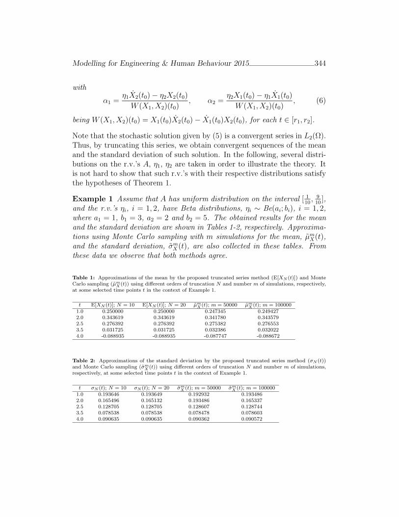
Modelling for Engineering & Human Behaviour 2015 344
with
α1 =η1X2(t0)− η2X2(t0)
W (X1, X2)(t0), α2 =
η2X1(t0)− η1X1(t0)
W (X1, X2)(t0), (6)
being W (X1, X2)(t0) = X1(t0)X2(t0)− X1(t0)X2(t0), for each t ∈ [r1, r2].
Note that the stochastic solution given by (5) is a convergent series in L2(Ω).Thus, by truncating this series, we obtain convergent sequences of the meanand the standard deviation of such solution. In the following, several distri-butions on the r.v.’s A, η1, η2 are taken in order to illustrate the theory. Itis not hard to show that such r.v.’s with their respective distributions satisfythe hypotheses of Theorem 1.
Example 1 Assume that A has uniform distribution on the interval [ 110, 9
10],
and the r.v.’s ηi, i = 1, 2, have Beta distributions, ηi ∼ Be(ai; bi), i = 1, 2,where a1 = 1, b1 = 3, a2 = 2 and b2 = 5. The obtained results for the meanand the standard deviation are shown in Tables 1-2, respectively. Approxima-tions using Monte Carlo sampling with m simulations for the mean, µmX(t),and the standard deviation, σmX (t), are also collected in these tables. Fromthese data we observe that both methods agree.
Table 1: Approximations of the mean by the proposed truncated series method (E[XN (t)]) and MonteCarlo sampling (µmX (t)) using different orders of truncation N and number m of simulations, respectively,at some selected time points t in the context of Example 1.
t E[XN (t)]; N = 10 E[XN (t)]; N = 20 µmX (t); m = 50000 µmX (t); m = 1000001.0 0.250000 0.250000 0.247345 0.2494272.0 0.343619 0.343619 0.341780 0.3435792.5 0.276392 0.276392 0.275382 0.2765533.5 0.031725 0.031725 0.032386 0.0320224.0 -0.088935 -0.088935 -0.087747 -0.088672
Table 2: Approximations of the standard deviation by the proposed truncated series method (σN (t))and Monte Carlo sampling (σm
X (t)) using different orders of truncation N and number m of simulations,respectively, at some selected time points t in the context of Example 1.
t σN (t); N = 10 σN (t); N = 20 σmX (t); m = 50000 σm
X (t); m = 1000001.0 0.193646 0.193649 0.192932 0.1934862.0 0.165496 0.165132 0.193486 0.1653372.5 0.128705 0.128705 0.128607 0.1287443.5 0.078538 0.078538 0.078478 0.0786034.0 0.090635 0.090635 0.090362 0.090572

Modelling for Engineering & Human Behaviour 2015 345
Example 2 Assume that A has a truncated beta distribution on [d,1-d] ,d = 1× 10⁻⁷, with parameters α = 1 and β = 3; η1 has a standard Gaussiandistribution, η1 ∼ N(0; 1) and η2 has with uniform distribution on [0, 1],η2 ∼ U ([0, 1]). From Tables 3-4 we observe a high agreement between bothapproximations.
Table 3: Approximations of the mean by the proposed truncated series method (E[XN (t)]) and MonteCarlo sampling (µmX (t)) using different orders of truncation N and number m of simulations, respectively,at some selected time points t in the context of Example 2.
t E[XN (t)]; N = 10 E[XN (t)]; N = 20 µmX (t); m = 50000 µmX (t); m = 1000001.0 0 0 0.005396 -0.0051132.0 0.293729 0.293729 0.297004 0.2893152.5 0.307795 0.307795 0.309329 0.3049803.5 0.147978 0.147978 0.146352 0.1489024.0 0.024559 0.024559 0.022073 0.026854
Table 4: Approximations of the standard deviation by the proposed truncated series method (σN (t))and Monte Carlo sampling (σm
X (t)) using different orders of truncation N and number m of simulations,respectively, at some selected time points t in the context of Example 2.
t σN (t); N = 10 σN (t); N = 20 σmX (t); m = 50000 σm
X (t); m = 1000001.0 1.000000 1.000000 1.004220 1.0023102.0 0.670807 0.670807 0.674305 0.6722272.5 0.364257 0.364257 0.366328 0.3647833.5 0.322779 0.322779 0.323623 0.3235594.0 0.484010 0.484010 0.485911 0.485238
A comparison of the CPU time used in Mathematica R© 7.0 to computesome numerical results presented in Tables 1-4 is shown in Table 5. Thesedata show that the proposed truncated series method is faster than the MonteCarlo Method.
Table 5: Execution time for computing the mean and variance for Examples 1 and 2 implemented on
Intel R© CoreTM
2 Duo, 4GB, 2.4GHz.
Methods Monte Carlo Truncated series method % Increase10× 104 simulations truncation order N=20
CPU(seconds) CPU(seconds)Example 1 94.30 31.46 300.2Example 2 94.32 3.49 2702.6
Modelling for Engineering & Human Behaviour 2015 346
3 Conclusions
In this paper mean square convergent generalized power series solution ofthe random Bessel differential equation (4) have been constructed takingadvantage of Lp-random calculus. The results obtained extend their deter-ministic counterpart under mild conditions. In addition, general expressionsto approximate both the mean and the variance of the solution have been de-termined. An important feature of our analysis is that these approximationsare guaranteed to converge to their respective exact values. To illustrate thereliability of the results, two examples have been provided. Finally, we wantto point out that our approach can be very useful to continue studying, froma probabilistic standpoint, other kind of Bessel differential equations.
Acknowledgements. This work has been partially supported by the Spanish Ministerio de Economıa
y Competitividad grant MTM2013-41765-P and by the European Union in the FP7-PEOPLE-2012-ITN
Program under Grant Agreement no. 304617 (FP7 Marie Curie Action, Project Multi-ITN STRIKE-Novel
Methods in Computational Finance) and Mexican Conacyt.
References
[1] F. E. Relton, Applied Bessel Functions, London, Blackie and Son Lim-ited, 1946.
[2] T. T. Soong, S. N. Chuang, , Solutions of a class of random differen-tial equations, SIAM Journal on Applied Mathematics 24 (4): 449–459,1973.
[3] M. El-Sohaly, Mean square convergent three and five points finite differ-ence scheme for stochastic parabolic partial differential equations, Elec-tronic Journal of Mathematical Analysis and Applications 2: 66–84,2014.
[4] T. T. Soong, Random Differential Equations in Science and Engineering,New York, Academic Press, 1973.
[5] L. Villafuerte, C. A. Braumann, J. C. Cortes, L. Jodar, Random dif-ferential operational calculus: Theory and applications, Computers andMathematics with Applications 59 (1): 115–125, 2010.
A stochastic capacitated lot sizing problemunder vendor managed inventory for the paper
industry
Lorena Polo[ ∗, David Escuın[, and David Cipres[
([) Aragon Institute of Technology,
Marıa Luna 7-8, 50018 Zaragoza, Spain
November 30, 2015
1 Introduction
Production lot-sizing has a great impact on inventory, particularly underseasonal fluctuations of demand and constrained production capacity. Manycompanies adopt the MTO (Make To Stock) policy in which products are notbuilt until a confirmed order for products is received by the manufacturer.Other companies maintain high levels of inventory (stock) to face periods ofuncertain demand. However, a production schedule which does not adjustaccurately the real demand may lead to overstocks for some products andstock-outs for other. Inventory sizing by product is especially important un-der uncertainty, when the inventory is necessary to guarantee a service levelin a stochastic environment. One of the integration practices that can con-tribute to reduce inventory in the supply chain is Vendor Managed Inventory(VMI). VMI programs allow for consumer demand information to be dissem-inated up the supply chain, thus mitigating upstream demand fluctuationsdue to the bullwhip effect [4] and [6] . Due to this demand anticipation,VMI may allow to reduce logistic and manufacturing costs, reduce overalllead-times, improve service level and reduce transportation costs.
∗e-mail: [email protected]
347
Modelling for Engineering & Human Behaviour 2015 348
The aim of this paper is to develop a mathematical model to seek themost effective inventory mix to face stochastic demand at minimum cost ina two-level supply chain. We focus on a multi-product dynamic lot-sizingproblem under stochastic demand subject to capacity and service level con-straints. Unlike previous studies, this model is executed to compare a MTOstrategy to a VMI partnership between the supplier and their customers [2].Both policies are developed within the model, and their results are comparedwithin the numerical application.
In the problem, a schedule of production orders is determined over theplanning horizon in order to minimize the inventory holding costs of thesupply chain, taking into consideration that the supplier is also responsibleof initiating the replenishment orders and deliveries of their customers ac-cording to the VMI partnership. The model also considers features such asservice level required, the production capacity at machine level, set up timeor product-machine allocation. The integration of stochastic demand in theproduction/inventory model is performed through the statistical distributionof the forecast accuracy. Historical data are analyzed to select the most suit-able forecasting model for each reference (also called SKU). The selectedmodel is triggered to forecast the demand during the rolling horizon.
The applicability of the proposed model is illustrated empirically usinga real case study: a paper manufacturing company that pursues to improvecustomer service level and supply chain inventory costs through a properproduction planning of their paper machines and a suitable VMI order re-plenishment schedule. A cost analysis of the supply chain inventory underdifferent service levels and under different adoption rates of VMI demon-strates the potential of this model to improve performance in the supplychain.
2 Methodology for the the paper industry
problem
The case study addressed in this paper is related with the supply chain forthe pulp and paper industry . The sector comprises companies that usewood as raw material and produce pulp, paper, board and other cellulose-based products. This work is focused in the two-echelon operations from themanufacturers (facilities that processes the raw material) and the customers
Modelling for Engineering & Human Behaviour 2015 349
that receives the paper and produces strong, lightweight cardboard boxes.The manufacturers must meet the customer’s requirements in terms of paperquality, wide and other paper properties. Several approaches are launched toschedule the production into the paper machines. Board must be dispatchedto the customers by different transport modes as in [3].
The study compares the performance of VMI and MTO strategies in thetwo-echelon serial supply chain with finite production capacity. The perfor-mance is investigated using difference equations forming a simulation model.The purpose of using simulation is to provide a simplified environment intowhich a number of situations and ideas can be tested. From the simulationoutputs, the effect of the strategies on manufacturing on-costs, inventoryholding costs and transport costs will be quantified and discussed.
As said before, with an MTO strategy, the manufacturer produces inresponse to a customer order, whereas the manufacturer produces in antici-pation of orders with an VMI strategy (see [1] and [5]). The paper industryconsidered in the use case triggers orders in a calendar agreed with the man-ufacturer (weekly or every two weeks). To calculate the size of the order, thecustomers estimate the demand during the lead time and dispatched as [7][8]. It cause large orders to cover the demand under the uncertainty. This isthe key aspect that VMI seeks to lower.
2.1 Overall architecture.
Firstly, at initial stages, it is necessary to analytically calculate the cus-tomers safety stock (how much extra stock that is maintained to mitigaterisk of stockouts due to uncertainties in supply and demand), the manufac-turer inventory, and fill rate for VMI and MTO strategies. They are basedon the lead time, the delay between the time the reorder point is reachedand renewed availability. This will be the starting point prior to adjust aiterative approach aimed at performing forecasting and optimization tasksiteratively following similar optimization as in [10]. The overall vision ofthe paper is reflected in the Figure 1 and is also generalized by [9]. Manu-facturers and customers provide qualitative and quantitative information toadopt the forecasting and decision models. Experts work in a collaborativeenvironment and demand forecasts and error estimates (an estimate of howfar actual demand may be from forecasted demand) feed the decision modelwhich optimizes the lot sizing (quantity of paper to be produced) of themanufacturers. Historical data stored at the manufactures and warehouses
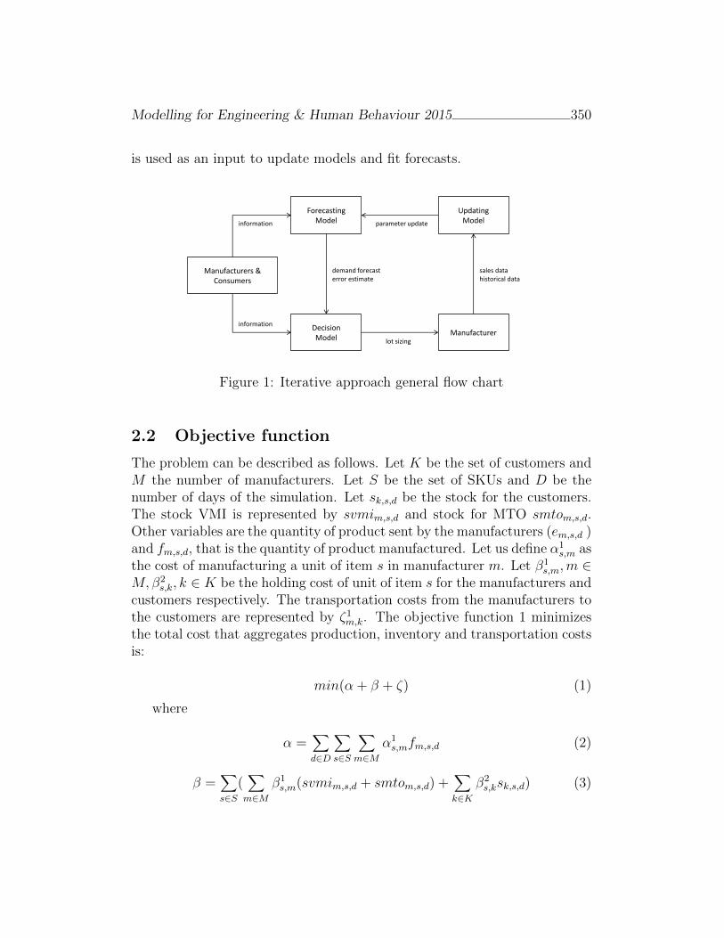
Modelling for Engineering & Human Behaviour 2015 350
is used as an input to update models and fit forecasts.
Forecasting Model
Manufacturers & Consumers
Decision Model
Updating Model
Manufacturer
information
information
demand forecast error estimate
sales data historical data
parameter update
lot sizing
Figure 1: Iterative approach general flow chart
2.2 Objective function
The problem can be described as follows. Let K be the set of customers andM the number of manufacturers. Let S be the set of SKUs and D be thenumber of days of the simulation. Let sk,s,d be the stock for the customers.The stock VMI is represented by svmim,s,d and stock for MTO smtom,s,d.Other variables are the quantity of product sent by the manufacturers (em,s,d )and fm,s,d, that is the quantity of product manufactured. Let us define α1
s,m asthe cost of manufacturing a unit of item s in manufacturer m. Let β1
s,m,m ∈M,β2
s,k, k ∈ K be the holding cost of unit of item s for the manufacturers andcustomers respectively. The transportation costs from the manufacturers tothe customers are represented by ζ1m,k. The objective function 1 minimizesthe total cost that aggregates production, inventory and transportation costsis:
min(α + β + ζ) (1)
where
α =∑d∈D
∑s∈S
∑m∈M
α1s,mfm,s,d (2)
β =∑s∈S
(∑m∈M
β1s,m(svmim,s,d + smtom,s,d) +
∑k∈K
β2s,ksk,s,d) (3)
Modelling for Engineering & Human Behaviour 2015 351
ζ =∑m∈M
∑k∈K
ζ1m,kem,k,s,d (4)
3 Conclusions
The work addresses the comparison between two replenishment policies. Theresults demonstrate the effectiveness of the model and the algorithms underVMI. The safety stock is reduced and, in turn, the inventory levels. Bytiming production and shipments, the manufacturer is able to manage theinventory level at the customers. VMI has proved to get a better performancethan MTO replenishment strategy. The paper simulates the VMI and tra-ditional supply chain MTO strategy in a scenario which previously has beenconfigured with the forecasted demand of the customer. During the rollinghorizon, the designed network of supply chain makes replenishment ordersto cover the forecasted demand with the objective of minimizing the totalcosts. It would be interesting to extend the model to address some aspectsmore deeply. How the shipments are scheduled based on the availability ofthe transport modes (rail of road transport) and the influence of the machinecycles derive on a great impact on the supply chain.
Acknowledgment
The dissemination of this work has been partly financed by the FSE Opera-tive Programme for Aragon (2007-2013).
References
[1] Disney, S.M. and Towill, D.R., 2003 The effect of VMI dynamics onthe bullwhip effect in supply chains, International Journal of Pro-duction Economics, Vol. 85, No. 2, pp199-215. DOI: 10.1016/S0925-5273(03)00110-5.
[2] Fraile, A. Larrode, E., Magrean, A. Sicilia, J.A. Decision model for sitingtransport and logistic facilities in urban environments: A methodologicalapproach. Journal of Computational and Applied Mathematics Volumen290: 100-120, 2015.
Modelling for Engineering & Human Behaviour 2015 352
[3] Gallego, J., Larrode, E., Sicilia, J.A., Royo, B. y Fraile, A. Optimizationand sizing methodology of necessary infraestructure for the incorpora-tion of hydrogen to the transportation sector. DYNA - Ingenierıa eIndustria., Volume 89: 405–412, 2014.
[4] Govindan, K. The optimal replenishment policy for time-varyingstochastic demand under vendor managed inventory. European Journalof Operational Research. Volume 242, Issue 2, 402-423, 2015.
[5] Johnson M., Eric, M., D, Tom. Vendor-managed inventory in the retailsupply chain Waller, Journal of Business Logistics; 1999; 20, 1; ProQuestBusiness Collection pg. 183
[6] Kwangyeol, R., Ilkyeong M., Seungjin O., Mooyoung J. A fractal echelonapproach for inventory management in supply chain networks. Interna-tional Journal of Production Economics Volume 143, Issue 2, 316-326.2013.
[7] Royo, B., Fraile, A., Larrode, E. y Muerza, M.V. Route planning fora mixed delivery system in long distance transportation and compari-son with pure delivery systems. Journal of Computational and AppliedMathematics. Volumen 291: 488-496. 2016.
[8] Royo, B. Sicilia, J.A., Oliveros, M.J., Larrode, E. Solving a Long-Distance Routing Problem using Ant Colony Optimization. AppliedMathematics & Information Sciences Volumen 9. 415-421. 2015.
[9] Peter A. Salzarulo. Vendor managed inventory programs and their effecton supply chain performance. Submitted to the faculty of the Univer-sity Graduate School in partial fulfillment of the requirements for thedegree Doctor of Philosophy in the Kelley School of Business. IndianaUniversity 2006.
[10] Sicilia, J.A., Royo, B., Quemada, C. Oliveros, M.J, Larrode, E. Andecision support system to long haul freight transportation by meansof ant colony optimization. DYNA - Ingenierıa e Industria. Volume 90:105-113. 2015.
A Tensor Bezier Shape Deformation forcluttered and uncertain spaces
L.Hilario[ ∗, A. Falco[, N. Montes†, F. Chinesta‡ and M.C.Mora
([) Cardenal Herrera University,
Departamento de Ciencias, Fısicas, Matematicas y de la Computacion
San Bartolome 55, 46115 Alfara del Patriarca (Valencia), Spain,
(†) Cardenal Herrera University,
Departamento de Ingenierıa de la Edificacion y Produccion Industrial
San Bartolome 55 46115 Alfara del Patriarca (Valencia), Spain,
(‡) Ecole Centrale Nantes,
Institut Universitaire de France
Nantes (France),
() Universitat Jaume I ,
Departamento de Ingenierıa Mecanica y Construccion
Avd. Vicent Sos Baynat s/n 12071 Castellon, Spain
November 30, 2015
1 AbstractIn this paper we propose an improvement of the Tensor Bezier Shape Deforma-tion algorithm developed in our previous work, [Hilario(2015]. In this case thealgorithm is applied in cluttered and uncertain spaces. The most common exam-ple of these spaces is the traffic congestion (cars, trucks and pedestrians) wherean automated system wants to guide you from a initial position to a final position.
353
Modelling for Engineering & Human Behaviour 2015 354
For instance how to cross a crowded square. In [Hilario(2015] a trajectory free ofcollisions of a mobile robot was computed obtaining the deformation of the ini-tial trajectory through a field of known vectors. The modified trajectory to avoidthe obstacles passes through these vectors. The improvement of the algorithmdeveloped in cluttered spaces looks for the more probable trajectory to cross thecluttered space in a safely manner. Some simulations are shown at the end of thepaper to illustrate the algorithm.
2 IntroductionThe aim of this study is how to guide a robot in a dynamic, cluttered and uncertainspace (DCUS). The problem in this situation is how the robot must work interact-ing with many robots or obstacles. If the space is uncertain or cluttered is difficultto predict the moviment of all of those. Our objective is how to obtain the optimaltrajectory of the mobile robot in a DCUS. An example of a DCUS is a square fullof cars and motorbikes, pedestrians! and the aim of this algorithm is to find thebest trajectory to cross this intersection avoiding all the obstacles.
Our previous work defined an algorithm based on the deformation of a Beziertrajectory through a field of vectors (forces). The consequence is how to guide amobile robot with a smooth trajectory free of collisions. DCUS represents betterthe real situation and our previous algorithm does not work fine in this realis-tics environments. In fact, our new algorithm will look for a preferred trajec-tory because it will be computed when possible. There are few works studyingthis situation, for example we can find [Toit(2012), Toit(2010)]. This publica-tion develops a procedure to approximately solve the stochastic dynamic prob-lem. Classical motion planning algorithms, [LaValle(2006)] mostly ignore un-certainty when planning in static or dynamic environments. When the future lo-cations of moving agents are known, the two common approaches are to add atime-dimension to the configuration space, or velocity tuning, [LaValle(2006)].When the future locations are unknown, the planning problems is either solvedlocally, [Burgard(1997), Fiorini(1998), Choset(2007)], or global planners guidesthe robot towards the goal and a local planner reacts to the dynamic componentof the environment, [LaValle(2006), Choset(2007), Clodic(2005)]. One of the at-tempt to extend the local planner to uncertain environments is the ProbabilisticVelocity Obstacle approach, [Fulgenzi(2008)].
[Toit(2010)] represents the first formal effort to incorporate the effect of antic-ipated future measurements in the motion planning process.
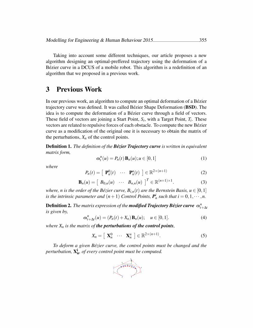
Modelling for Engineering & Human Behaviour 2015 355
Taking into account some different techniques, our article proposes a newalgorithm designing an optimal-preffered trajectory using the deformation of aBezier curve in a DCUS of a mobile robot. This algorithm is a redefinition of analgorithm that we proposed in a previous work.
3 Previous WorkIn our previous work, an algorithm to compute an optimal deformation of a Beziertrajectory curve was defined. It was called Bezier Shape Deformation (BSD). Theidea is to compute the deformation of a Bezier curve through a field of vectors.These field of vectors are joining a Start Point, Si, with a Target Point, Ti. Thesevectors are related to repulsive forces of each obstacle. To compute the new Beziercurve as a modification of the original one it is necessary to obtain the matrix ofthe perturbations, Xn of the control points.
Definition 1. The definition of the Bezier Trajectory curve is written in equivalentmatrix form,
αnt (u) = Pn(t)Bn(u);u ∈ [0,1] (1)
wherePn(t) =
[P0
n(t) · · · Pnn(t)
]∈ R2×(n+1) (2)
Bn(u) =[
B0,n(u) · · · Bn,n(u)]T ∈ R(n+1)×1. (3)
where, n is the order of the Bezier curve, Bi,n(t) are the Bernstein Basis, u ∈ [0,1]is the intrinsic parameter and (n+1) Control Points, Pi
n such that i = 0,1, · · · ,n.
Definition 2. The matrix expression of the modified Trajectory Bezier curve αnt+∆t
is given by,αn
t+∆t(u) = (Pn(t)+Xn)Bn(u); u ∈ [0,1]. (4)
where Xn is the matrix of the perturbations of the control points,
Xn =[
X0n · · · Xn
n]∈ R2×(n+1). (5)
To deform a given Bezier curve, the control points must be changed and theperturbation, Xi
n, of every control point must be computed.
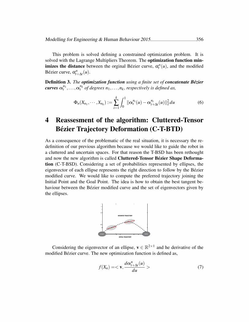
Modelling for Engineering & Human Behaviour 2015 356
This problem is solved defining a constrained optimization problem. It issolved with the Lagrange Multipliers Theorem. The optimization function min-imizes the distance between the orginal Bezier curve, αn
t (u), and the modifiedBezier curve, αn
t+∆t(u).
Definition 3. The optimization function using a finite set of concatenate Beziercurves αn1
t , . . . ,αnkt of degrees n1, . . . ,nk, respectively is defined as,
Φn(Xn1 , · · · ,Xnk) :=k
∑i=1
∫ 1
0‖αni
t (u)−αnit+∆t(u)‖
22 du (6)
4 Reassesment of the algorithm: Cluttered-TensorBezier Trajectory Deformation (C-T-BTD)
As a consequence of the problematic of the real situation, it is necessary the re-definition of our previous algorithm because we would like to guide the robot ina cluttered and uncertain spaces. For that reason the T-BSD has been rethoughtand now the new algorithm is called Cluttered-Tensor Bezier Shape Deforma-tion (C-T-BSD). Considering a set of probabilities represented by ellipses, theeigenvector of each ellipse represents the right direction to follow by the Beziermodified curve. We would like to compute the preferred trajectory joining theInitial Point and the Goal Point. The idea is how to obtain the best tangent be-haviour between the Bezier modified curve and the set of eigenvectors given bythe ellipses.
START% GOAL%
INITIAL&TRAJECTORY&
MODIFIED&TRAJECTORY&
Considering the eigenvector of an ellipse, v ∈ R2×1 and he derivative of themodified Bezier curve. The new optimization function is defined as,
f (Xn) =< v,dαn
t+∆t(u)du
> (7)

Modelling for Engineering & Human Behaviour 2015 357
considering < ., . > the scalar euclidean product.If we want to obtain the best tangent between the Bezier curve and the eigen-
vector of the ellipse, we should maximize this function.
5 ConclusionsThe critical situations for the autonomous systems are the cluttered and uncertainspaces. It is difficult to predict the movements of the humans and the movementsof obstacles when the path planning is solved in a congested environment. Wehave defined an initial framework to look for the preferred trajectory between aInitial Point and a Goal Point guiding the autonomous system trying to be freeof collisions. A preferred Bezier trajectory is defined computing the best tangentbetween the ellipses and the modified Bezier Trajectory.
References[Toit(2012)] N.E.Du Toit, and J.W. Burdick: Robot Motion Planning in Dynamic
Uncertain Environments. IEEE Transactions on Robotics, Vol. 28, NO. 1,February 2012.
[Toit(2010)] N.E.Du Toit and J.W. Burdick: Robot Motion Planning in Dy-namic, Cluttered, Uncertain Environments. IEEE International Conferenceon Robotics and Automation, May 2010.
[LaValle(2006)] S.M. LaValle: Planning Algorithms. Cambridge UniversityPress, 2006.
[Burgard(1997)] D. Fox, W. Burgard and S. Thrun: The dynamic window ap-proach to collision avoidance. IEEE Robotics and Automation Magazine,Vol.4, no.1, pp. 23-33, 1997.
[Fiorini(1998)] P. Fiorini and Z. Shiller: Motion planning in dynamic environ-ments using velocity obstacles. International Journal of Robotics Research,Vol. 17, no. 7, pp. 760-722, July 1998.
[Choset(2007)] H. Choset, K.M.Lynch, S. Hutchinson, G. Kantor, W. Burgard,L.E.Kavraki and S. Thrun: Principles of Robot Motion. MIT Press, 2007.

Modelling for Engineering & Human Behaviour 2015 358
[Clodic(2005)] A. Clodic, V. Montreuil, R. Alami and R. Chatila: A decisionalframework for autonomous robots interacting with humans. IEEE Interna-tional Workshop on Robot and Human Interactive Communication, August2005, pp. 543-548.
[Fulgenzi(2008)] C. Fulgenzi, A. Spalanzani and C. Laugier, Dynamic obstacleavoidance in uncertain environment combining pvos and occupancy grid.IEEE International Conference on Robotics and Automation, April 2007.
[Hilario(2015] Hilario L., Falco A., Montes N., Mora M.C. A tensor optimiza-tion algorithm for Bezier Shape Deformation. Journal of Computational andApplied Mathematics, doi: 10.1016/j.cam.2015.02.035.
Closed-form formulae vs. PDE basednumerical solution for FRAP data processing:
Theoretical and practical comparison
S. Papacek[ ∗, B. Macdonald†, and C. Matonoha‡
([) University of South Bohemia in C. Budejovice, Institute of Complex Systems, FFPW,
Zamek 136, 373 33 Nove Hrady, Czech Republic,
(†) University of Glasgow, School of Mathematics and Statistics,
Glasgow, G12 8QW, Scotland,
(‡) Institute of Computer Science, Academy of Sciences of the Czech Republic,
Pod Vodarenskou vezı 2, 182 07 Prague 8, Czech Republic.
November 30, 2015
1 Introduction
Fluorescence recovery after photobleaching (FRAP) is a widely used methodto analyse (usually using fluorescence microscopy) the mobility of either flu-orescently tagged or autofluorescent proteins (e.g., photosynthetic) in livingcells. The FRAP method works by imaging the recovery of fluorescenceintensity over time in a region of interest previously bleached by a high-intensity laser pulse. Whilst the basic principles of FRAP are simple andthe experimental setup is usually fixed, quantitative FRAP data analysis isnot well developed. Several models and numerical procedures are used forthe underlying model parameter estimation, i.e., the data processing step isnot currently well established. Hence, a natural inquiry: Are all FRAP dataprocessing methods well suited?
∗e-mail: [email protected]
359
Modelling for Engineering & Human Behaviour 2015 360
In this paper we rigorously formulate the inverse problem of model pa-rameter estimation (including the sensitivity analysis) making possible thecomparison of different FRAP data processing methods. Then, in a casestudy with simulated datasets, we focus on how different methods for data(pre)processing influence the error in parameter estimation. We explain whyour new method based on a general initial-boundary value problem formula-tion for the Fick diffusion PDE should exhibit less bias and narrower confi-dence intervals of the estimated model parameters, than other state-of-the-artmethods.
2 Model parameter estimation based on spatio-
temporal data
We aim to determine both the model parameter value p ∈ Rq, q ∈ N, and thecorresponding confidence interval, subject to the noise in data and a quantityrelated to the sensitivity, see (4). The data are represented by a (measured)signal on a Cartesian product of the space-points (xi)
ni=1 and time-points
(tj)mj=1. Let NData := m × n be the total number of spatio-temporal data
points. We define the operator S : Rq → RNData that maps parameter valuesp1, . . . , pq to the solution of the underlying initial-boundary value problem,e.g. (5), evaluated at points (xi, tj): S(p) = y(xi, tj, p) ∈ R, 1 ≤ i ≤n, 1 ≤ j ≤ m.
It is common in the FRAP community to perform a preprocessing, e.g.,space averaging [4], or not to employ all the NData measured values at points(xi, tj), i = 1, . . . , n, j = 1, . . . ,m [6]. Hence we define the observation op-erator G : RNData → RNdata that evaluates the set of values S(p) on a certainsubset of the full data space (Ndata ≤ NData): G(S(p)) = (z(xl, tl, p))
Ndata
l=1
The forward map F = G S, representing the parameter-to-output map-ping, is defined as the composition of the PDE solution operator S and theobservation operator G; F : p→ z(xl, tl, p)
Ndatal=1 . Our regression model is now
F (p) = data. (1)
The data are modelled and contaminated with additive Gaussian noise.Given some data, the aim of the parameter estimation problem is to find
pT , such that (1) is satisfied in some appropriate sense. Since (1) usuallyconsists of an overdetermined system (there are more data points than un-
Modelling for Engineering & Human Behaviour 2015 361
knowns), it cannot be expected that (1) holds with equality, but instead anappropriate notion is that of a least-squares solution p
‖ data− F (p) ‖2= minp‖ data− F (p) ‖2 . (2)
Fisher information matrix and confidence intervals
For the sensitivity analysis we require the Frechet-derivative F ′[p1, . . . , pq] ∈RNdata×q of the forward map F , that is
F ′[p1, . . . , pq] =(
∂∂p1F (p1, . . . , pq), . . . , ∂
∂pqF (p1, . . . , pq)
).
A corresponding quantity is the Fisher information matrix (FIM)
M [p1, . . . , pq] = F ′[p1, . . . , pq]TF ′[p1, . . . , pq] ∈ Rq×q. (3)
Using [1], we can estimate confidence intervals. Suppose we have computedp as the least-squares solution in (2), we can then define the residual asres2(p) = ‖F (p)− data‖2 =
∑Ndata
i=1 [datai − z(xi, ti, p)]2 . Then according to
[1], it is possible to quantify the error between the computed parameters pand the true parameters pT .
With the further comparison of certain methods of FRAP data processingin mind, we restrict ourselves on one single scalar parameter p estimation.Then, the Fisher information matrix M in (3) reduces into the scalar quan-
tity∑Ndata
i=1
[p ∂∂pz(xi, ti, p) |p=p
]2(corresponding to the semi-relative sensitiv-
ity and the estimate of the relative parameter error variance). The 1 − αconfidence interval for the observations, where α is the significance level, isthen described as follows
(p− pTp
)2Ndata∑i=1
[p∂
∂pz(xi, ti, p) |p=p
]2≤ res2(p)
Ndata − 1f1,Ndata−1(α), (4)
where f1,Ndata−1(α) corresponds to the upper α quantile of the Fisher distri-
bution with 1 and Ndata − 1 degrees of freedom. Notice the term res2(p)Ndata−1
is
an estimator of the error variance, such that the approximation res2(p)Ndata−1
∼ σ2
holds if Ndata is large [1].
Modelling for Engineering & Human Behaviour 2015 362
3 Comparison of several FRAP data process-
ing methods
The fluorescence intensity measured in a region of interest Ω is proportionalto the concentration of non-bleached particle’s cnb. It holds cnb
c+ cb
c= 1, where
cb is the bleached particles concentration, and c is the overall concentration.The Fick diffusion equation holds for both variables, cnb and cb respectively.Hence, for the sake of simplicity, we further study the spatio-temporal dy-namics of the fraction cb
c:= y, as a function of one spatial coordinate x, time
t and diffusion coefficient p
∂y
∂t− p∂
2y
∂x2= 0 , (5)
in (t0, T )× Ω, with suitable boundary conditions on (t0, T )× ∂Ω and initialconditions in Ω, where Ω ⊂ R, being the bleached particles distribution justafter the bleaching.
The one-point Mullineaux method
C. W. Mullineaux et al. [6] measured one-dimensional bleaching profilesalong the specimen long axis. They took the initial bleaching profile (ofbleached particles) as a Gaussian with half-width r0 at height (or depth)y0,0e
−2, i.e., the initial condition in the form of
y(x, t0) = y0,0 exp−2x2
r02, (6)
where t0 corresponds to the time instant just after bleaching and can be setto zero. For the infinite domain, i.e., x ∈ R, the solution y(x, t, p) of (5) is
y(x, t, p) =y0,0 r0√r02 + 8pt
exp−2x2
r02 + 8pt, x ∈ R, t ∈ [0, T ]. (7)
In order to determine the diffusion coefficient, Mullineaux et al. [6] tookonly the time evolution of the normalized fluorescence intensity in the centerof the bleached area (x = 0), i.e., z(t) := y(0, t, p)/y0,0, where the maximumbleached level is reached. Continuing with our terminology developed in Sec-tion 2, we have zM(t, p) = r0√
r02+8pt, and the corresponding FIM, based on the
Modelling for Engineering & Human Behaviour 2015 363
semi-relative sensitivities and normalized output (divided by the maximumvalue y0,0), collapses to the scalar quantity
MM =m∑j=1
[p∂zM(tj, p)
∂p
]2=
m∑j=1
(4r0ptj)2
(r02 + 8ptj)3=
1
4
m∑j=1
(8sj)2
(1 + 8sj)3, (8)
where we introduced the dimensionless variable sj :=ptjr02
.
Initial boundary value problem for (5) and the FIMcalculation
As the closed-form formulae approaches have several limitations or inaccu-racies, we propose to model the diffusion process by the Fick diffusion equa-tion with realistic initial and boundary conditions instead, e.g., as an initialboundary value problem (5-6). The parameter estimation is then formulatedas an ordinary least squares problem (2) resulting in the estimate pPDE, seee.g., [7, 4].
The uncertainty assessment of the estimate pPDE is based on the numer-ical evaluation of FIM. For each time instant tj we denote pj = pPDE, oursoftware CA-FRAP solves (5) and using the simulated output y(xi, tj, pj), i =1, . . . , n., according to (3), evaluates the FIM (diagonal in this case).
Our examples on simulated FRAP datasets show an agreement with thetheoretical prediction for the low data noise levels (for signal-to-noise ratiountil 30) only. FRAP data analysis is a challenging problem and a recentresearch direction, and scaling up to larger noise scenarios is work in progress.
Conclusion: We have developed a unified modelling framework for pro-cessing of FRAP data sets in order to compare two basic approaches ofthe fluorescent compounds mobility determination from the spatio-temporalFRAP measurement. The first and simplest approach is based on the curvefitting to a closed-form formula and obviously needs some unrealistic or hard-to-accomplish conditions. The second approach is based on a numerical ap-proximation of the Fick diffusion PDE (5). Both approaches are implementedin our software CA-FRAP, which advantageously uses the UFO (UniversalFunctional Optimization) system [5]. CA-FRAP simultaneously provides theparameter estimate and the corresponding standard error (with is therebyused to calculate the confidence interval).
Modelling for Engineering & Human Behaviour 2015 364
Acknowledgements
This work was supported by the MEYS of the Czech Republic - projects CE-NAKVA (No. CZ.1.05/2.1.00/01.0024), CENAKVA II (No. LO1205 underthe NPU I program), and by the long-term strategic development financingof the Institute of Computer Science (RVO:67985807).
References
[1] Bates D. M., and Watts D. G. Nonlinear regression analysis: Its appli-cations. New York, John Wiley & Sons, 1988.
[2] Cintron-Arias A., Banks H. T., Capaldi A., and Lloyd A. L. A sensitivitymatrix based methodology for inverse problem formulation. J. Inv. Ill-Posed Problems, Volume (17):545–564, 2009.
[3] Ellenberg J., et al. Nuclear membrane dynamics and reassembly in livingcells: targeting of an inner nuclear membrane protein in interphase andmitosis. The Journal of Cell Biology, Volume (138):1193-1206, 1997.
[4] Kindermann, S., and Papacek, S. On Data Space Selection and DataProcessing for Parameter Identification in a Reaction-Diffusion ModelBased on FRAP Experiments. Abstract and Applied Analysis, Volume(2015):17 pp., Article ID 859849, 2015.
[5] L. Luksan, M. Tuma, C. Matonoha, J. Vlcek, N. Ramesova, M. Siska,and J. Hartman, UFO 2014 - Interactive system for universal func-tional optimization. Technical Report V-1191, Institute of ComputerScience, Academy of Sciences of the Czech Republic, Prague 2014(http://www.cs.cas.cz/luksan/ufo.html).
[6] Mullineaux C. W., Tobin M. J., and Jones G. R. Mobility of photo-synthetic complexes in thylakoid membranes. Nature, Volume (390):421-424, 1997.
[7] Papacek S., Kana R., and Matonoha C. Estimation of diffusivity ofphycobilisomes on thylakoid membrane based on spatio-temporal FRAPimages. Mathematical and Computer Modelling, Volume (57):1907–1912,2013.

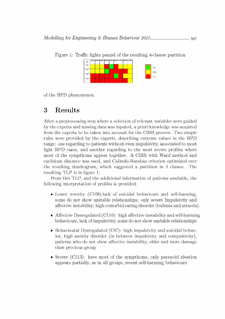
Related Documents