Modelling fluxes of water and sediment between Venice Lagoon and the sea

ARTICLE IN PRESS

Continental Shelf Research 30 (2010) 904–914

Contents lists available at ScienceDirect

Continental Shelf Research

0278-43

doi:10.1

� Corr

E-m

(A. Cucc

cnr.it (D

journal homepage: www.elsevier.com/locate/csr

Modelling fluxes of water and sediment between Venice Lagoon and the sea

Christian Ferrarin a,�, Andrea Cucco b, Georg Umgiesser a, Debora Bellafiore a,c, Carl L. Amos d

a Institute of Marine Science, National Research Council (ISMAR-CNR), Castello 1364/a, 30122 Venice, Italyb Institute for the Coastal Marine Environment, National Research Council (IAMC-CNR), Oristano, Italyc EuroMediterranean Centre for Climate Change (CMCC), Bologna, Italyd National Oceanography Centre (NOCS), Southampton, UK

a r t i c l e i n f o

Article history:

Received 5 February 2009

Received in revised form

5 July 2009

Accepted 25 August 2009Available online 4 September 2009

Keywords:

Finite element model

Venice Lagoon

Tidal inlets

Sand transport

43/$ - see front matter & 2009 Elsevier Ltd. A

016/j.csr.2009.08.014

esponding author. Tel.: +39 412404772; fax:

ail addresses: [email protected] (C. Ferrar

o), [email protected] (G. Umgiess

. Bellafiore), [email protected] (C.L. Amo

a b s t r a c t

To describe the exchange of water and sediment through the Venice Lagoon inlets a 3-D hydrodynamic

and sediment transport model has been developed and applied to a domain comprising Venice Lagoon

and a part of the Adriatic Sea. The model has been validated for both current velocities and suspended

particle concentration against direct observations and from observations empirically derived fluxes

from upward-looking acoustic Doppler current profiler probes installed inside each inlet. The model

provides estimates of the suspended sediment transport in the lower 3 m of the water column that is

not detected by acoustic Doppler current profiler sensors. The bedload model prediction has been

validated against measured sand transport rates collected by sand traps deployed in the Lido and

Chioggia inlets. Results indicate that, in the Lido inlet, 87% of the total load is in suspension, while the

rest moves as bedload.

& 2009 Elsevier Ltd. All rights reserved.

1. Introduction

Coastal lagoons are shallow water bodies partially isolatedfrom the adjacent sea by a sedimentary barrier and connected to itthrough one or several tidal inlets. The hydrodynamic behavior inthese coastal systems, even if is driven mainly by tide, is verycomplicated since this area contains a lot of different processes.Model applications could be useful in understanding the mainphysical processes, since a complete field datasets is hard toobtain.

The main purpose of this study is to investigate the dynamicsof the Venice Lagoon inlets in order to simulate the fluxes of waterand sediment between the lagoon and the sea (Fig. 1). Threejettied inlets, situated at the eastern boundary of the lagoon,exchange waters between the northern Adriatic Sea and thelagoon.

The sediment transport between the lagoon and the sea, andits effects on the morphology, is of crucial importance in themanagement of many aspects regarding the safeguarding of thelagoon environment and the city of Venice. The order ofmagnitude of the loss of sediment (especially fines) is stilldebated Carbognin and Cecconi (1997), Sarretta et al. (this issue)and Defendi et al. (this issue).

ll rights reserved.

+39 415204126.

in), [email protected]

er), debora.bellafiore@ismar.

s).

Fine sediments in the inner lagoon is mainly resuspended bywind generated waves and then transported by the tidal currents(Tambroni and Seminara, 2006; Carniello et al., 2005; Ferrarinet al., 2008). As discussed by Umgiesser et al. (2004b), the waveeffects of the bottom stress is negligible for the inlet regions ofVenice Lagoon and, even during severe storms, wave induced set-up in the lagoon is small compared to the wind induced set-up(Roland et al., in press; Nguyen et al., 2007). Moreover, since theinlets are placed a few hundred meters away from the shore, areduced amount of sediment resuspended by wave breaking inthe surf zone would be able to reach the inlets during the floodphase (Tambroni and Seminara, 2006). These previous findingsallow us to exclude the waves when simulating the inletsdynamics.

In the last decade, several numerical models have been appliedto provided a detailed pictures of the inlets dynamics using 1-Dand 2-D approaches. Bellafiore et al. (2008) applied a 2-D finiteelement hydrodynamic model over a spatial domain comprisingboth the Adriatic Sea and the Venice Lagoon to simulate the waterexchange between the sea and the lagoon. The good agreementbetween modelled and measured fluxes at the inlets demon-strated the efficiency of the model to reproduce tide-inducedwater exchanges between the sea and the lagoon basin.

Tambroni and Seminara (2006) applied a simple model of theinlet hydrodynamics to estimate the net exchange of sandassociated with the sequence of tidal events. As a result of their1-D sediment transport model they concluded that the yearly lossof sand though the Venice inlets is in the order of0:1� 106 m3 yr�1. As well, modelling by Umgiesser et al. (2006)

www.elsevier.com/locate/csr

dx.doi.org/10.1016/j.csr.2009.08.014

mailto:[email protected]







ARTICLE IN PRESS

Fig. 1. Bathymetry of the Venice Lagoon obtained by using the grid of the

numerical model, superimposed. Circles mark the location of the tidal gauges.

Diamonds indicate the location of the fixed ADCP in the inlets. A black square

marks the oceanographic tower Acqua Alta.

C. Ferrarin et al. / Continental Shelf Research 30 (2010) 904–914 905

indicates an export of sand from the lagoon through Lido inletthrough erosion of the major tidal channels.

These previous modelling studies lack a detailed verticalresolution of currents in the inlets for an adequate computationof the bed shear stresses that are fundamental in the estimation ofsuspended and bedload transport rates. The objective of this workis to provide, using a 3-D model, quantification of water andsediment fluxes through the Venetian inlets, also within the lower3 m of the water column that is not detected by the fixed ADCPsensors. It is therefore a preliminary step to a more ambitiousgoal, the quantification of the sediment budget through numericalmodelling. This estimation will be the topic of a forthcomingpaper, where also the wave model will be applied inside theVenice Lagoon.

2. Study area

Venice Lagoon, a coastal system located in the NorthwestAdriatic Sea (Fig. 1), covers roughly an area of 500 km2; its majoraxis is oriented north-east to south-west. It is characterized by acomplicated network of channels, intertidal flats and shoals. A fewprincipal deep channels (maximum depth around 15 m) cross anarea of very shallow water with an average depth on the order of1 m. The three inlets are called, from north to south, Lido,Malamocco and Chioggia and are from about 500 to about 900 mwide and up to 15 m deep.

All three inlets, Lido, Malamocco and Chioggia, are fixed bylong jetties. The construction of jetties has definitely enhanced the

degree of ebb-flood asymmetry experienced by the flow field inthe near-inlet region, suggesting that a net exchange of sedimentsthrough the inlet in each tidal cycle may be driven by purelyhydrodynamic factors (Tambroni and Seminara, 2006).

The main driving forces for water circulation within the lagoonare the tide (about 1 m excursion during spring tides) and thewind. The tide propagates into the lagoon along the deep, narrowchannels onto the tidal flats and tidal marshes.

Due to the high tidal energy and relatively shallow water, thewater masses are generally well mixed (Umgiesser et al., 2004a).In particular inside the inlets, where the water velocities are high(over 1 m s�1), vertical shear creates enough turbulence to mix thewater column (Gacic et al., 2002). Stratification of water massesoccurs only in the inner lagoon where the tidal energy isattenuated. Consequently the water exchanges between thelagoon and the sea that are driven mainly by the tide and thewind action, are essentially barotropic in nature (Gacic et al.,2002). Over 90% of the total variance in the average water fluxthrough the inlets is due to tidal forcing and the amount of marinewater that flows in and out during each tidal cycle amounts toabout a third of the total volume of the lagoon (Gacic et al., 2004).

Sediment features are affected by hydrodynamics with coarsermaterials in the proximity of the inlets and tidal channelsand finer materials in mudflats and salt marshes (Molinaroliet al., 2007).

3. Description of the models

The unstructured grid-based numerical model used in thisstudy is a coupled 3-D current and sediment transport modelworking simultaneously on a common finite element grid. The3-D hydrodynamic finite element model SHYFEM (Umgiesser,1997) solves the shallow water equations with a semi-implicitalgorithm that is unconditionally stable for gravity waves. At eachtime step, the resulting 3-D model computes for every node of thenumerical domain the water level and the current velocities ineach layer. Thereafter the sediment transport rate model SED-TRANS05 (Neumeier et al., 2008) computes the erosion anddeposition rates and determines the suspended sediment volumein the bottom model layers for several sediment sizes. Finally,suspended sediment transport is computed by means of atransport and diffusion module whereas the bedload sedimenttransport is computed by means of a direct advection scheme.

The 2-D version of the morphodynamic model has beenextensively described in Ferrarin et al. (2008). Here we reporton the extended 3-D model formulation.

3.1. The hydrodynamic model

The hydrodynamic model SHYFEM here applied has beendeveloped at ISMAR-CNR (Institute of Marine Science-National

Research Council) (Umgiesser and Bergamasco, 1995; Umgiesser etal., 2004a). The model uses finite elements for horizontal spatialintegration and a semi-implicit algorithm for integration in time.The finite element method is highly flexible due to the subdivisionof the numerical domain in triangles varying in form and size. It isespecially suited to reproduce the geometry and the hydrody-namics of complex shallow water basins such as Venice Lagoonwith its narrow channels and small islands.

Velocities are computed in the center of each element, whereasscalars are computed at each mode. Vertically the model appliesZ layers with varying thickness. Most variables are computed inthe center of each layer, whereas stress terms and verticalvelocities are solved at the interfaces between layers.

ARTICLE IN PRESS

C. Ferrarin et al. / Continental Shelf Research 30 (2010) 904–914906

The model resolves the primitive equations, vertically inte-grated on each layer. The horizontal diffusion, the baroclinicpressure gradient and the advective terms in the momentumequation are treated fully explicitly. The Coriolis force and thebarotropic pressure gradient terms in the momentum equationand the divergence term in the continuity equation are semi-implicitly treated. The vertical stress terms and the bottomfriction term are treated fully implicitly for stability reasons dueto the very shallow nature of the lagoon. The discretization resultsin unconditional stability which is essential for modelling theeffects of fast gravity waves, bottom friction and the Coriolisacceleration (Umgiesser and Bergamasco, 1995). For the computa-tion of the vertical diffusivities and viscosities a turbulenceclosure scheme has been used. This scheme is an adaptation of thek–e module of GOTM (general ocean turbulence model) describedin Burchard and Petersen (1999).

The equations, integrated on each layer, are

@Ul

@tþul

@Ul

@xþvl

@Ul

@y� fV l ¼ � ghl

@z@x�

ghl

r0

@

@x

Z z

�Hl

r0 dz

�hl

r0

@pa

@xþ

1

r0

ðttopðlÞx � tbottomðlÞ

x ÞþAH@2Ul

@x2þ@2Ul

@y2

� �ð1Þ

@Vl

@tþul

@Vl

@xþvl

@Vl

@yþ fUl ¼ � ghl

@z@y�

ghl

r0

@

@y

Z z

�Hl

r0 dz

�hl

r0

@pa

@yþ

1

r0

ðttopðlÞy � tbottomðlÞ

y ÞþAH@2Vl

@x2þ@2Vl

@y2

� �ð2Þ

@z@tþX

l

@Ul

@xþX

l

@Vl

@y¼ 0 ð3Þ

with l indicating the vertical layer, (Ul;Vl) the horizontal transportat each layer (integrated velocities), f the Coriolis parameter, pa

the atmospheric pressure, g the gravitational acceleration, z thesea level, r0 the average density of sea water, r¼ r0þr0 the waterdensity, t the internal stress term at the top and bottom of eachlayer, hl the layer thickness, Hl the depth of the bottom of layer l,AH the horizontal eddy viscosity.

The boundary conditions for stress terms are

tsurfacex ¼ cDrawx

ffiffiffiffiffiffiffiffiffiffiffiffiffiffiffiffiffiw2

xþw2y

q; tsurface

y ¼ cDrawy

ffiffiffiffiffiffiffiffiffiffiffiffiffiffiffiffiffiw2

xþw2y

qð4Þ

tbottomx ¼ cBr0uL

ffiffiffiffiffiffiffiffiffiffiffiffiffiffiffiu2

Lþv2L

q; tbottom

y ¼ cBr0vL

ffiffiffiffiffiffiffiffiffiffiffiffiffiffiffiu2

Lþv2L

qð5Þ

where cD is the wind drag coefficient, cB is the bottom frictioncoefficient, ra is the air density, ðwx;wyÞ are the zonal andmeridional components of the wind velocity, respectively, andðuL; vLÞ is the water velocity in the lowest layer.

At the lateral open boundaries of the domain, the water levelsare prescribed while at the closed boundaries the normal velocityis set to zero and the tangential velocity is a free parameter. Thiscorresponds to a full slip condition. The model also simulatesflooding and drying of the shallow water flats. This is especiallyimportant in Venice Lagoon, because the intertidal area coversabout 15% of the lagoon at low water spring tide conditions. Theflooding and drying mechanism has been implemented in a massconsistent way, and spurious oscillations that are generated arequickly damped. When the water levels fall below a threshold of5 cm, the element is removed from the computation, and watermass is conserved to compute water levels at every time step witha Laplacian interpolation. The element is reintroduced into thecomputation when the interpolated water level values are higherthan a second threshold of 10 cm. The wet and dry mechanismand its implementation into the model is fully described inUmgiesser et al. (2004a).

3.2. The sediment transport model

The sediment transport model SEDTRANS05 (Neumeier et al.,2008) simulates erosion and sedimentation rates under eithersteady currents or the combined and time-dependent influence ofwaves and currents.

The model adopts the Grant and Madsen (1986) continental shelfbottom boundary layer theory to predict bed shear stresses and thevelocity profile in the bottom boundary layer. The velocity computedby the 3-D hydrodynamic model in the bottom layer is used tocalculate the bed shear stress. SEDTRANS05 provides five formula-tions to predict sediment transport for non-cohesive sediments: themethods of Brown (1950), Yalin (1963) and Van Rijn (1993) predictthe bedload transport; the methods of Engelund and Hansen (1967)and Bagnold (1963) predict the total load transport.

Multiple grain sizes are used to track changes in seabedtexture, and differential transport of material. At each location, thebed is modeled as several layers, the uppermost of themrepresents the surficial active, or mixed, layer. For each size class,the volume of sediment removed from the bed during any timestep is limited by the amount available in the active layer. In thisway the model takes into account time-dependent and spatialsediment distribution and bed armoring.

Further details on the sediment transport algorithm forcohesive and sandy sediments are given in Neumeier et al.(2008) and Ferrarin et al. (2008).

The 3-D formulation of the advection–diffusion equation forsuspended sediment reads

@Sl

@tþ@ulSl

@xþ@vlSl

@yþ@ðwl �wsÞSl

@z¼ nh

@2Sl

@x2þ@2Sl

@y2

� �þnv;l

@2Sl

@z2þF

ð6Þ

where Sl is the suspended sediment concentration (SSC) in thelayer l, nh and nv;l are the horizontal and vertical turbulentdiffusion coefficients, respectively, and ws is the (positive) settlingvelocity. The term F represents external source terms. Thisequation conserves sediment mass that is advected with currents,deposits due to gravity and diffuses due to turbulence.

Vertical boundary conditions for the advection–diffusionequation are

þnv;top@Stop

@zþwsStop ¼ 0; z¼ top of the surface layer

�nv;bot@Sbot

@zþwsSbot ¼ ED; z¼ bottom of the lowest layer ð7Þ

where ED is the net sediment water column-bottom flux,corresponding to the difference between resuspension anddeposition for each grain class.

The vertical mixing coefficients nv;l are calculated by the k–eturbulence closure model.

4. Application to Venice Lagoon

4.1. The simulation set-up

The hydrodynamic numerical computation has been carried outon a spatial domain that represents Venice Lagoon and the shore infront of the lagoon by means of a grid that consists of 17278 nodesand 31910 triangular elements (Fig. 1). Only a small part of thenorthern Adriatic Sea (up to 15 km offshore) has been used incomputation in order to reduce the computational time. Additionallythis choice is connected with the handling of the wind forcing. In factthe implementation described in Bellafiore et al. (2008) applied theECMWF wind dataset over the entire Adriatic Sea, which suffer a

ARTICLE IN PRESS

Table 1Physical parameters used in the simulations.

Parameter Description Value

cD Wind drag coefficient 2:5� 10�3

r0 Average water density 1025 kg m�3

ra Air density 1:225 kg m�3

AH Horizontal viscosity 0 m2 s�1

Dt Max. time step 300 s

Current veloci0

2

4

6

8

10

12

0.8

0.6

0.4

0.2

0

-0.2

-0.4

Wat

er le

vel [

m]

04:00 08:00 1time

0 0.2 0.4Current v

Dep

th [m

]

AD

CP S

hadow zone

Fig. 2. Measured and modelled velocity profiles at Lido inlet during a tida

Table 2Statistical analysis of water simulated level for the year 2006.

Tide gauge RMSE BIAS SI R2

DSL 2.7 �0.4 0.10 0.995

DNM 2.8 �0.1 0.10 0.995

DSC 3.1 1.7 0.12 0.985

PS 2.2 �0.3 0.12 0.997

BUR 4.4 �0.1 0.17 0.987

MUR 3.1 1.2 0.12 0.995

SAL 2.7 1.2 0.11 0.997

CHI 3.9 2.9 0.15 0.995

Average 3.1 0.8 0.12 0.993

Analysis results are given in terms of RMSE (root mean square error) in cm, BIAS

(difference between mean of the observations and simulations) in cm, SI (scatter

index), and R2 (correlation coefficient).


general under-estimation in speed (Zampato et al., 2007). In thepresent work, the choice of a limited computational domain allowsone to use measured data collected at the Oceanographic TowerAcqua Alta (black square in Fig. 1) instead of using the low resolutionmeteorological modelled dataset. This improves the accuracy ofwind forcing especially in the region of the Venice Lagoon.

The inlet configurations include the infrastructures related tothe Mo.S.E project (from the Italian acronym for ‘‘ExperimentalElectromechanics Module’’) to defend the city of Venice and thesurrounding lagoon from high water events. The project entailsbuilding mobile barriers at the bottom of each inlet which, whenflood events threaten to become critical, will rise and shut off thelagoon from the sea. The main changes around the Lido inlet arethe construction of an artificial island in the middle of the inlet,the dredging of a new channel behind this new island and thecreation of two safety harbors in the sides of the channel. In theother two inlets (Malamocco and Chioggia), outer breakwatershave been built in the sea near the inlets and safety harbors havebeen created at the sides of the channels (Fig. 1).

The use of elements of variable sizes, typical of finite elementmethods, was fully exploited, in order to suit the complicatedgeometry of the basin, the rapidly varying topographic features,and the complex bathymetry.

The bathymetric data adopted for this study was collected in2000. In this application the water column has been discretizedinto 17 vertical layers with variable thickness ranging from 1 m, inthe topmost 10 m, to 7 m for the deepest layer of the outer shelf.

ty profile at Lido

2:00 16:00 [hours]

20:00

0.6 0.8 1elocity [m/s]

1.2

ADCPModel

MeasuredModel

06:0009:0011:0013:0016:0019:0022:00

Oce

an D

ata

View

l cycle. Corresponding water level variation is shown on the bottom.

ARTICLE IN PRESS


All simulations were forced by observed values of windrecorded inside the lagoon and offshore at the OceanographicTower Acqua Alta. Open boundaries are treated by definingobserved water levels at the Oceanographic Tower Acqua Alta. Inthis paper the baroclinic contribution is not considered thereforethe model results takes into account only the water exchangesbetween the lagoon and the sea induced by the tide and windaction. Hydrodynamic model parameters used in the simulationare listed in Table 1.

Seven grain-size classes of non-cohesive sediment rangingfrom medium to very fine sand, and 11 classes in the silt andclay ranges were prescribed. The grain size distribution ofbottom sediments has been mapped onto the finite elementgrid from more than 100 field samples (Magistrato alleAcque-Consorzio Venezia Nuova (MAV-CVN), 1999). Grain sizedistributions were considered to be homogeneous within eachsediment layer.

-9000-6000-3000

0 3000 6000 9000

Dis

char

ge [m

3 s-1

] ADCP Model

0.00.20.40.60.81.01.21.41.6

Velo

city

[m s

-1]

0.00.20.40.60.81.01.21.41.6

Velo

city

[m s

-1]

0.00.20.40.60.81.01.21.41.6

Velo

city

[m s

-1]

0.00.20.40.60.81.01.21.41.6

172 173 174

Velo

city

[m s

-1]

tim

Fig. 3. Time series of computed (dotted line) and measured (continuous line) current vel

shown on the top.

The critical erosion threshold and surface sediment density inVenice Lagoon have been found to be seasonally and spatiallyhighly variable. Amos et al. (2004) investigated the stability oftidal flats in Venice Lagoon in two surveys during summer 1998and subsequent winter, using two annular flumes: Sea Carouseland Mini Flume. The measured lagoon-averaged values of tce was1.77 Pa in the intertidal zone and 0.70 Pa in the subtidal zone.Amos et al. (2004) showed that the critical erosion thresholdcould be predicted from sediment bulk density. Due to its spatialvariability across the lagoon, the surface sediment densitydistribution has been initialized with field data collected overthe whole lagoon (Magistrato alle Acque-Consorzio VeneziaNuova (MAV-CVN), 1999).

In this study only the van Rijn algorithm is applied, becauseprevious studies (Neumeier et al., 2008; Villatoro et al., this issue)showed that it yields the best results for Venice inlets.

All simulations presented in this work are for the year 2006.

BIN

2 [2

m]

BIN

5 [5

m]

BIN

8 [8

m]

175 176 177 178

BIN

10

[10

m]

e [days]

ocity at different depth in the Lido inlet. Corresponding water discharge variation is

ARTICLE IN PRESS


4.2. Validation data

4.2.1. ADCP data

A seabed mounted, upward-looking, fixed ADCP was installedin each of the three tidal inlets of Venice Lagoon (Gacic et al.,2004; Kovacevic et al., 2008) (diamonds in Fig. 1). This type ofinstallation acquires current velocities and acoustical backscatter,which is calibrated to suspended particle concentration. Thepurpose of these installations is to study the time-dependentvariability of inlet currents, water exchange rates, and net residualsediment transports.

During a pilot phase that comprised neap and spring tides,about 100 ship-borne ADCP surveys were conducted to establish astatistical relationship between the vertically averaged watervelocities collected with the bottom mounted ADCP and the inletcross-sectional flow rates. Gacic et al. (2004, 2002) found that the10-min flow rates could be predicted with a precision of 97% (95%

Table 3Statistical analysis of simulated current velocity in the inlets for the year 2006 at

different depths.

Inlet Depth RMSE BIAS SI R2

Lido Top (2 m) 19.1 1.6 0.35 0.83

Bottom (10 m) 14.5 �4.1 0.31 0.87

Malamocco Top (2 m) 12.3 6.2 0.22 0.96

Bottom (18 m) 7.9 0.1 0.17 0.96

Chioggia Top (2 m) 18.9 �5.0 0.34 0.86

Bottom (7 m) 12.0 0.8 0.31 0.86

Analysis results are given in terms of RMSE (root mean square error) in cm s�1,

BIAS (difference between mean of the observations and simulations) in cm s�1, SI

(scatter index), and R2 (correlation coefficient).

0

0.01

0.02

0.03

0.04

0.05

00:00 04:00 08:00 12:00 16:00 2

Fric

tion

Velo

city

[m2

s-1]

Time

Lido Inlet (19-20/09/2006)

0

0.01

0.02

0.03

0.04

0.05

0.06

0.07

0.08

00:00 04:00 08:00 12:00 16:00 2

Fric

tion

Velo

city

[m2

s-1]

Time

Chioggia Inlet (13-14/07/2007)

Fig. 4. Bottom friction velocity derived from near bed ADV velocity (dots), vertically me

layer (dotted line).

confidence level) using a linear transfer function. In this way,empirically related fluxes can be provided at high temporalresolution.

Parameters of an inverse model to derive suspended sedimentconcentrations from ADCP backscatter intensities were tuned bymeans of corresponding water samples taken at various depth atthe moorings and during the ship surveys. The estimate of thehourly concentration uncertainty is about 3 mg l�1 (Defendi et al.,this issue).

The suspended solid flux from the bed-mounted ADCP isobtained from the hourly concentration estimates multiplied bythe discharge. The suspended sediment concentrations arevertically averaged values and refer to the portion of watercolumn above the fixed ADCP. Cross-sectional flux obtained fromvessel surveys is computed from the suspended sedimentconcentrations averaged over the transect crossing the inlet andpassing over the position of the bed-mounted ADCP. Theuncertainty on the total solid transport, computed using themethod of error propagation, was about 16% at the 95% confidencelevel (Kovacevic et al., 2007; Defendi et al., this issue).

4.2.2. Sand trap data

Sand transport rates at the Lido (2006) and Chioggia(2006, 2007 and 2008) inlets were measured using Helley–Smithsediment traps, equipped with 60mm nets. Modified Helley–Smith sand traps and a surface sampler were deployed synchro-nously from a boat for periods of 20 min duration. TwoHelley–Smith samplers sat on the bed in benthic (bedload,0ozo0:12 m) and epibenthic (0:21ozo0:33 m) modes. A thirdsampler was fixed to the vessel near the surface. The samplescovered a wide range of current velocities over both the flood andebb phases of the tide.

0:00 00:00 04:00 08:00 12:00 16:00 [hours, UT]

ADVModel 2DModel 3D

0:00 00:00 04:00 08:00 12:00 16:00 [hours, UT]

ADVModel 2DModel 3D

an velocity from 2-D model (continuous line) and velocity from the last 3-D model

ARTICLE IN PRESS


Additional data collection at Lido (2006) and Chioggia (2007)sites consisted of near bed current velocity (0.34 m above the bed)measured with a acoustic Doppler velocimeter (ADV) mounted ona frame that was lowered to the bed. See Amos et al. (in press) andVillatoro et al. (this issue) for further details and discussion on thesand trap and surveys methodology.

5. Results and discussion

The 3-D hydrodynamic model has been validated for thefollowing key variables:

�
propagation of the tidal wave by comparison with observedwater levels; � magnitude of modelled friction velocity by comparison with
observed current magnitudes and vertical current profiles;
� mass exchange at the inlets by comparison with observed and
empirically related fluxes.

The sediment transport model has been tested and modelresults are compared against:

�
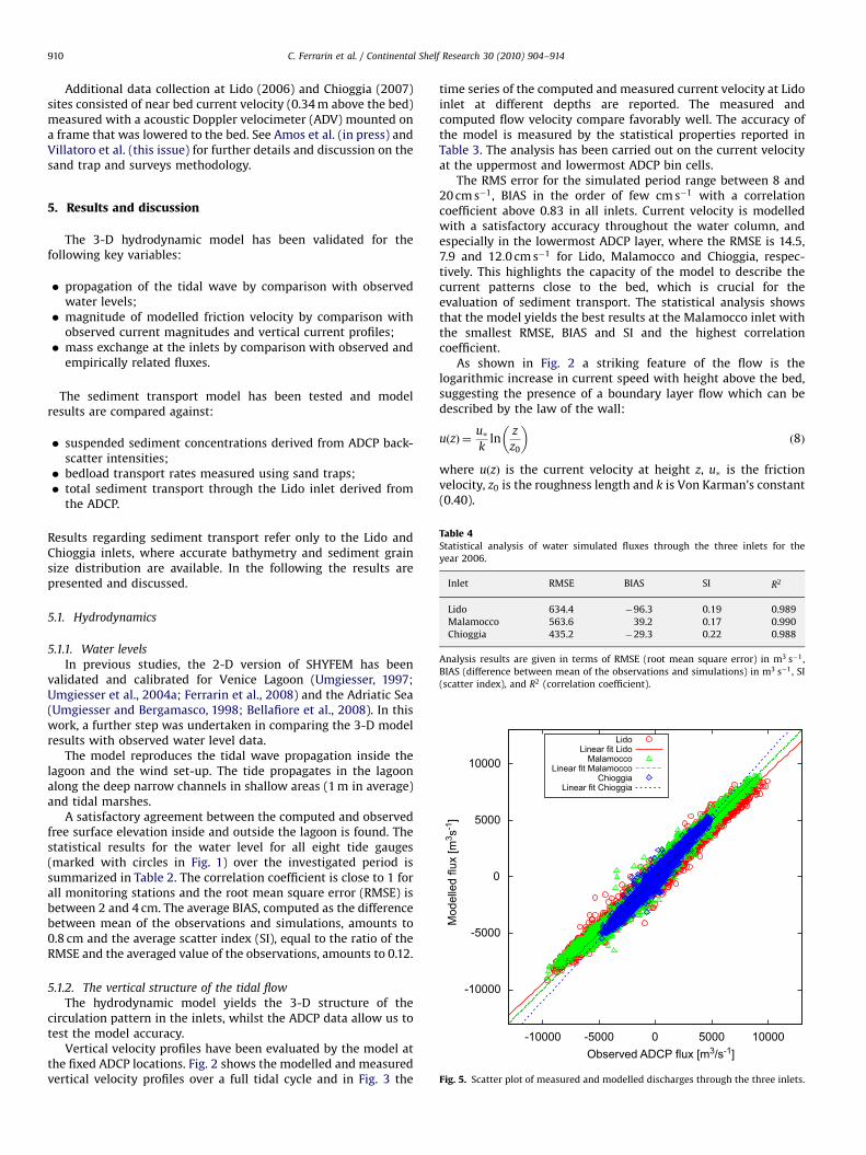
suspended sediment concentrations derived from ADCP back-scatter intensities; � bedload transport rates measured using sand traps; �
Table 4Statistical analysis of water simulated fluxes through the three inlets for the

year 2006.

Inlet RMSE BIAS SI R2

Lido 634.4 �96.3 0.19 0.989

Malamocco 563.6 39.2 0.17 0.990

Chioggia 435.2 �29.3 0.22 0.988

Analysis results are given in terms of RMSE (root mean square error) in m3 s�1,

BIAS (difference between mean of the observations and simulations) in m3 s�1, SI

(scatter index), and R2 (correlation coefficient).

-10000

-5000

0

5000

10000

-10000 -5000 0 5000 10000

LidoLinear fit Lido

MalamoccoLinear fit Malamocco

ChioggiaLinear fit Chioggia

Mod

elle

d flu

x [m

3 s-1

]

Observed ADCP flux [m3/s-1]

Fig. 5. Scatter plot of measured and modelled discharges through the three inlets.

total sediment transport through the Lido inlet derived fromthe ADCP.

Results regarding sediment transport refer only to the Lido andChioggia inlets, where accurate bathymetry and sediment grainsize distribution are available. In the following the results arepresented and discussed.

5.1. Hydrodynamics

5.1.1. Water levels

In previous studies, the 2-D version of SHYFEM has beenvalidated and calibrated for Venice Lagoon (Umgiesser, 1997;Umgiesser et al., 2004a; Ferrarin et al., 2008) and the Adriatic Sea(Umgiesser and Bergamasco, 1998; Bellafiore et al., 2008). In thiswork, a further step was undertaken in comparing the 3-D modelresults with observed water level data.

The model reproduces the tidal wave propagation inside thelagoon and the wind set-up. The tide propagates in the lagoonalong the deep narrow channels in shallow areas (1 m in average)and tidal marshes.

A satisfactory agreement between the computed and observedfree surface elevation inside and outside the lagoon is found. Thestatistical results for the water level for all eight tide gauges(marked with circles in Fig. 1) over the investigated period issummarized in Table 2. The correlation coefficient is close to 1 forall monitoring stations and the root mean square error (RMSE) isbetween 2 and 4 cm. The average BIAS, computed as the differencebetween mean of the observations and simulations, amounts to0.8 cm and the average scatter index (SI), equal to the ratio of theRMSE and the averaged value of the observations, amounts to 0.12.

5.1.2. The vertical structure of the tidal flow

The hydrodynamic model yields the 3-D structure of thecirculation pattern in the inlets, whilst the ADCP data allow us totest the model accuracy.

Vertical velocity profiles have been evaluated by the model atthe fixed ADCP locations. Fig. 2 shows the modelled and measuredvertical velocity profiles over a full tidal cycle and in Fig. 3 the

time series of the computed and measured current velocity at Lidoinlet at different depths are reported. The measured andcomputed flow velocity compare favorably well. The accuracy ofthe model is measured by the statistical properties reported inTable 3. The analysis has been carried out on the current velocityat the uppermost and lowermost ADCP bin cells.

The RMS error for the simulated period range between 8 and20 cm s�1, BIAS in the order of few cm s�1 with a correlationcoefficient above 0.83 in all inlets. Current velocity is modelledwith a satisfactory accuracy throughout the water column, andespecially in the lowermost ADCP layer, where the RMSE is 14.5,7.9 and 12:0 cm s�1 for Lido, Malamocco and Chioggia, respec-tively. This highlights the capacity of the model to describe thecurrent patterns close to the bed, which is crucial for theevaluation of sediment transport. The statistical analysis showsthat the model yields the best results at the Malamocco inlet withthe smallest RMSE, BIAS and SI and the highest correlationcoefficient.

As shown in Fig. 2 a striking feature of the flow is thelogarithmic increase in current speed with height above the bed,suggesting the presence of a boundary layer flow which can bedescribed by the law of the wall:

uðzÞ ¼u�k

lnz

z0

� �ð8Þ

where uðzÞ is the current velocity at height z, u� is the frictionvelocity, z0 is the roughness length and k is Von Karman’s constant(0.40).

ARTICLE IN PRESS


Identifying the existence of a log-layer is important because itprovides one way to estimate the bottom stress. The fitting ofmeasured velocity profiles to the logarithmic form (Eq. (8)) is triedin a least-square sense starting with the lowest three data pointsfollowing the approach of Lueck and Lu (1997). The error in thefitting is calculated as the maximum magnitude of the differencebetween the fitted values of uðzÞ and the observed data at eachvelocity bin. For a fit to be acceptable we require that this error isless than 1% of the maximum speed of the bins involved.

The fitting was tried with 52 561 velocity profiles collected inthe Lido inlet and covering the whole 2006 year. The profilingrange obtained for the Lido inlet was from 2.9 to 11.0 m above thebed. Only 21.5% of the velocity profiles can be fitted with a log-layer. The remaining 78.5% have a log-layer height less than 4.9 m,or no log-layer at all. To exclude the period around slack water, the

-40

-20

0

20

40

60

80

Wat

er le

vel [

m]

Observed Modelled

0

10

20

30

SS

C [m

g/l]

ADCP Model

0

10

20

30

SS

C [m

g/l]

0

10

20

30

SS

C [m

g/l]

0

10

20

30

172 173 174 1

SS

C [m

g/l]

time

Fig. 6. Time series of computed (dotted line) and measured (continuous line) suspende

level variation is shown on the top.

analysis has been successively restricted to situations represent-ing sediment transport stage, which has been defined when thecurrent speed in the lowest bin exceed the critical velocity at thatdepth. Friction velocity at 2.9 m above the bottom has beenevaluated using Eq. (8) and considering the site specific criticalfriction velocity for sediment movement found by Amos et al. (inpress) (0:017 m s�1); 30 716 velocity profiles result to be in thetransport stage and only 35.3% of them can be fitted with a log-layer.

From these results we argue that in principle the bottomboundary properties of this site could not be performed scalingthe vertically mean velocities from a 2-D model.

To highlight the real need of a 3-D approach a comparativecase study has been performed. ADV near bed (0.34 m above thebed) current velocity, vertically mean velocities from the 2-D

BIN

2 [2

m]

BIN

5 [5

m]

BIN

8 [8

m]

75 176 177 178

BIN

10

[10

m]

[days]

d sediment concentration at different depth in the Lido inlet. Corresponding water

ARTICLE IN PRESS

1e-05

1e-04

1e-03

1e-02

1e-01

1e+00

1e-05 1e-04 1e-03 1e-02 1e-01 1e+00

Qb

Com

pute

d [k

g/m

s]

Lido 06Chioggia 06Chioggia 07Chioggia 08

Qb Measured [kg/ms]

Fig. 7. Measured and computed sediment transport rates in Chioggia and Lido

inlets according to Van Rijn methods. Solid line indicates perfect agreement and

dashed lines represent factor 2 area.

Table 5Validation of the non-cohesive transport equation using 3-D model: percentage of

predicted value within factor 2 of measured values.

Dataset Number of samples Model results (%)

Lido 2006 10 50

Chioggia 2006 10 40

Chioggia 2007 11 45

Chioggia 2008 8 50


model and velocity from the last 3-D model layer (1 m above thebed) has been used to estimate the friction velocity throughEq. (8) using a roughness length of 0.002 m (Amos et al., in press).As shown in Fig. 4 the 3-D model reproduces the bottom frictionvelocity more accurately than the 2-D model. The friction velocityderived from 2-D model is underestimated in both Lido andChioggia cases during the ebb phase, revealing the limit of thisapproach in reproducing tidal flow in the inlets.

5.1.3. Water fluxes

Once the model was validated against water levels andvelocities, it was used to estimate the water exchange throughthe three inlets. Modelled fluxes through the inlets are comparedwith the empirically derived water discharges from the mooredADCP. The model reproduces the fluxes through the inlets with acorrelation coefficient larger than 0.98 in all cases and a RMSE of634.4, 563.6 and 435:2 m3 s�1 for Lido, Malamocco and Chioggiainlet respectively (Table 4). The accuracy of the model is measuredadditionally by the scatter index (SI) and BIAS. The SI amounts to0.17 at Malamocco, 0.19 at Lido and 0.22 at Chioggia. The BIASamounts to �96:3, 39.2, �29:3 at Lido, Malamocco and Chioggiainlet, respectively. Fig. 5 shows that the model matches well theempirical fluxes at Malamocco inlet, while slightly under-estimates the fluxes at Lido inlet and slightly over-estimatesthem at Chioggia inlet.

5.2. Sediment transport

Both suspended and bedload sediment transport is simulatedby the model over the whole computational domain. Suspendedsediment concentration profiles and bedload transport rates wereextracted for comparison at the bottom-mounted ADCP and sandtrap sampling locations.

5.2.1. Suspended sediment concentration profile

Time series of empirical and modelled SSC for the Lido inletduring a calm period of 2006 is shown in Fig. 6. The modelreproduces the sediment resuspension patterns that mimics thetidal cycle, revealing that, in calm conditions, sediments aregenerally resuspended locally by the tidal currents.

Modelled suspended sediment concentration decreases withheight above the bed suggesting a Rouse like vertical profile. Onthe other hand, empirically derived suspended particle concen-tration shows lower values on the deepest cell with respect to thecell above. The model underestimates the observed SSC, especiallyin the uppermost layers of the water column. This deviation isconsistent with the effects of the organic matter and phytoplank-ton on the acoustic backscatter intensity. Amos et al. (in press)reports that the material in the benthic boundary layer of theinlets is largely inorganic (495%); above this layer, organiccontent varied widely and is greatest near the surface. Discre-pancies between observation and model results could also be dueto the turbulent vertical exchange and settling velocities para-metrization.

5.2.2. Bedload sediment transport

Bedload sediment transport rate datasets are analyzedtogether. Even if they have been collected in different years anddifferent locations they are representative of similar tidalcondition. The seabed at both Chioggia and Lido sites is dominatedby well to moderately well sorted fine sand.

The comparison between measured and computed (using theVan Rijn algorithm) rates of sediment transport is shown in Fig. 7.The results are expressed in terms of the discrepancy ratio (r)defined as the ratio of the predicted and measured transport rate.

Table 5 shows the percentage of r values of the two datasetsfalling in the range of 0:5rrr2.

Between 40% and 50% of predicted values fall within a factor 2of the measured values. Scatter in the Chioggia 2006 datasetreflects the high uncertainty of the bedload algorithm at lowtransport stages. As shown in Fig. 7, the model tends to under-estimate the bedload transport rates at higher transport stage(Chioggia 2007 dataset).

5.2.3. Total sediment transport through the Lido inlet

A first attempt to describe the total sediment transportthrough the Lido inlet is presented. Modelled cross-sectionalfluxes of suspended solids were obtained by summing up the SSCtransports through each cell of the cross-section.

Fig. 8a shows the comparison between the total sedimenttransport in suspension computed by the model and the solid fluxderived from the ADCP (both bed-mounted and vessel-mounted).During low and moderate water speed conditions the modelledsediment fluxes match the observations. Around mid-ebb tide themodel predictions exceed observations systematically. Thisoverestimation during mid-ebb could be due to the fact thatthe model provides information on sediment transport within thelower portion of the water column that is not detected bythe ADCP sensors and where sediments concentration is greatest.This would suggest that 40% of the total sediment flux is found inthe lowest 3 m of the inlet water column.

The model estimates the bedload transport through the inlet atthe fixed ADCP site (Fig. 8b). Results show that sediment transport

ARTICLE IN PRESS

-200

-100

0

100

200

300

400a

b

Sol

id tr

ansp

ort d

isch

arge

[kg/

s]

ModelBed-ADCP

Vessel-ADCP

-200

-100

0

100

200

300

400

Sol

id tr

ansp

ort d

isch

arge

[kg/

s]

SuspendedBedload

-0.2 0

0.2 0.4 0.6 0.8

12:0019/09/06

18:00 00:00 06:00 12:0020/09/06

18:00 00:00 06:00 12:0021/09/06

Wat

er le

vel [

m]

Time [GMT]

Fig. 8. (a) Computed total suspended sediment transport (solid line) and empirical, from bed-mounted ADCP (dashed line) and vessel-mounted ADCP (dots) total

suspended solid transport at the Lido inlet and (b) modelled total suspended and bedload sediment transport through the Lido inlet. Corresponding water level variation is

shown on the bottom.


through Lido inlet is mostly in suspension (83%), while bedloadrepresents only a fraction of the total sediment transport (17%).Similar results have been found for most major rivers of the world,wherein approximately 10% of the total load is transported asbedload (Geophysics Study Committee and National GeographicSociety, 1994).

In general, for both suspension and bedload, the sediment fluxis positive, indicating a tendency for the loss of sediments fromthe lagoon.

6. Conclusions

In this study a 3-D hydrodynamic finite element modelcoupled with a sediment transport model have been applied toreproduce the water and sediment fluxes through the VeniceLagoon inlets. Comparison of model results with observations inthe area showed that the model could reproduce the majorfeatures of both hydrodynamic and sediment transport in the inletregion.

Both observations and model results reveal that the waterexchanges between the lagoon and the sea are driven mainly bythe tide and that, in the case of calm conditions, sediments in theinlet region are generally resuspended locally by tidal currents.

To examine the vertical character of the tidal flow in the Lidoinlet, the bottom mounted ADCP velocities were fitted to alogarithmic profile. Even if currents in the inlet regions are mainlybarotropic, the vertical structure of the tidal flow shows theabsence of a thick log-profile during most of the time. Conse-quently, a 3-D model approach is needed to represent correctly

the near bed current field. The comparison of the modelledfriction velocity with that derived from near bed ADV measure-ments showed that the 3-D approach reproduces the bottomboundary properties more accurately than the vertically inte-grated formulation.

Model results showed that sediment transport through Lidoinlet occurs mostly in suspension, while bedload represents only afraction of the total sediment transport. The model allows theprediction of the sediment transport within the near bed layerswhich cannot be permanently investigated by means of instru-mentations, such as ADCP. Therefore, the adopted numericalmodel can be considered as the suitable tool both for monitoringthe ongoing lagoon morphological changes and for predicting thepotential changes induced by the lagoon inlets modificationrelated to the Mo.S.E project.

To estimate the net sediment budget (total suspended andbedload) for Venice Lagoon there is a need to further improve themodelling chain. Especially in the case where during stormyconditions sediments are resuspended inside the lagoon, it is nottrue anymore that the sediments are only resuspended locally inthe inlets. In this case a 3-D fully coupled current, wave andsediment model is needed. This model is under development andwill be applied to investigate the long shore transport in front ofthe Venice Lagoon and its influence on the inlet morphodynamics.

Acknowledgments

This research was partially funded by the VECTOR project, Line5 CLIVEN: Aspetti dei cambiamenti climatici sulla Laguna di Venezia

ARTICLE IN PRESS


(case history), and by Ministero delle Infrastrutture e dei Trasporti-Magistrato alle Acque di Venezia, through Co.Ri.La, under theresearch program La Laguna di Venezia nel quadro dei cambiamenti

climatici, delle misure di mitigazione ed adattamento e dell’evolu-

zione degli usi del territorio. The authors wish to thank MiroslavGacic, Isaac Mancero Mosquera and Vedrana Kovacevic forproviding ADCP dataset and Luca Zaggia and Valentina Defendifor providing solid flux data. The wind and water level datasetshave been provided by the Venice Municipality.

References

Amos, C.L., Cappucci, S., Begamasco, A., Umgiesser, G., Bonardi, M., Cloutier, D.,Flindt, M., DeNat, L., Cristante, S., 2004. The stability of tidal flats in VeniceLagoon—the results of in situ measurements using two benthic annular flumes.Journal of Marine Systems 51, 211–241.

Amos, C.L., Villatoro, M., Rachel, H., Zaggia, L., Umgiesser, G., Venturini, V., Are, D.,Sutherland, T.A., Mazzoldi, A., Rizzetto, F., in press. The measurement of sandtransport in two inlets of Venice lagoon, Italy. Estuarine, Coastal and Shelf Science.

Bagnold, R.A., 1963. Mechanics of Marine Sedimentation. In: Hill, M.N. (Ed.), TheSea, vol. 3; 1963, pp. 265–305.

Bellafiore, D., Umgiesser, G., Cucco, A., 2008. Modelling the water exchangesbetween the Venice Lagoon and the Adriatic Sea. Ocean Dynamics 58, 397–413.

Brown, C.B., 1950. In: Rouse, H. (Ed.), Engineering Hydraulics.Burchard, H., Petersen, O., 1999. Models of turbulence in the marine environ-

ment—a comparative study of two equation turbulence models. Journal ofMarine Systems 21, 29–53.

Carbognin, L., Cecconi, G., 1997. The lagoon of Venice, environment, problems, andremedial measures. In: Field Guide of IAS Environmental SedimentologyConference, Venice. Consiglo Nationale della Ricerca, Venice, p. 71.

Carniello, L., Defina, A., Fagherazzi, S., D’Alpaos, L., 2005. A combined wind wave-tidalmodel for the Venice Lagoon, Italy. Journal of Geophysical Research 110, F04007.

Defendi, V., Kovacevic, V., Zaggia, L., Arena, F., this issue. Estimating sedimenttransport from acoustic measurements in the Venice Lagoon inlets. Con-tinental Shelf Research.

Engelund, F., Hansen, E., 1967. A Monograph on Sediment Transport in AlluvialStream. Teknisk Vorlag, Copenhagen, Denmark.

Ferrarin, C., Umgiesser, G., Cucco, A., Hsu, T.-W., Roland, A., Amos, C.L., 2008.Development and validation of a finite element morphological model forshallow water basins. Coastal Engineering 55 (9), 716–731.

Gacic, M., Kovacevic, V., Mazzoldi, A., Paduan, J.D., Arena, F., Mosquera, I.M., Gelsi, G.,Arcari, G., 2002. Measuring water exchange between the Venetian lagoon and theopen sea. EOS, Transaction, American Geophysical Union 83 (20), 217–222.

Gacic, M., Mosquera, I.M., Kovacevic, V., Mazzoldi, A., Cardin, V., Arena, F., Gelsi, G.,2004. Temporal variations of water flow between the Venetian lagoon and theopen sea. Journal of Marine Systems 51 (1–4), 33–47.

Geophysics Study Committee and National Geographic Society, 1994. MaterialFluxes on the Surface of the Earth. National Academy Press.

Grant, W.D., Madsen, O.S., 1986. The continental shelf bottom boundary layer.Annual Review of Fluid Mechanics 18, 265–305.

Kovacevic, V., Fendi, V.D., Arena, F., Gacic, M., Mosquera, I.M., Zaggia, L., Don�a, S.,Costa, F., Simionato, F., Mazzoldi, A., 2008. Water and solid transport estimatesthrough the Venetian Lagoon inlets using acoustic Doppler current profilers.

In: Scientific Research and Safeguarding of Venice. Research Program2004–2006. 2006 Results, vol. VI. CORILA, pp. 423–439.

Kovacevic, V., Fendi, V.D., Zaggia, L., Costa, F., Arena, F., Simionato, F., Mazzoldi, A.,Gacic, M., Amos, C.L., 2007. Time series of suspended particle concentrationfrom the conversion of acoustic backscatter at the Lido Inlet. In: ScientificResearch and Safeguarding of Venice. Research Program 2004–2006. 2005Results, vol. V. CORILA, pp. 315–339.

Lueck, R.G., Lu, Y., 1997. The logarithmic layer in a tidal channel. Continental ShelfResearch 14, 1785–1801.

Magistrato alle Acque-Consorzio Venezia Nuova (MAV-CVN), 1999. Mappaturadell’inquinamento dei fondali lagunari, studi e indagini. Rapporto finale.Technical Report OP 128, cap. 2, 4.1, 4.3.

Molinaroli, E., Guerzoni, S., Sarretta, A., Cucco, A., Umgiesser, G., 2007. Linksbetween hydrology and sedimentology in the Lagoon of Venice, Italy. Journal ofMarine Systems 68 (3–4), 303–317.

Neumeier, U., Ferrarin, C., Amos, C.L., Umgiesser, G., Li, M.Z., 2008. Sedtrans05: animproved sediment-transport model for continental shelves and coastalwaters. Computers & Geosciences 34 (10), 1223–1242.

Nguyen, X.T., Tanaka, H., Nagabayashi, H., 2007. Wave setup at River and InletEntrances Due to an Extreme Event. In: Proceedings of InternationalConference on Violent Flows, Organized by RIAM, Kyushu University, Fukuoka,Japan.

Roland, A., Cucco, A., Ferrarin, C., Hsu, T.-W., Liau, J.-M., Umgiesser, G., Zanke, U.,in press. On the development and verification of a 2d coupled wave-currentmodel on unstructured meshes. Journal of Marine System.

Sarretta, A., Molinaroli, E., Guerzoni, S., Fontolan, G., Pillon, S., this issue.Sediment budget in the Lagoon of Venice. Continental Shelf Research,doi:10.1016/j.csr.2009.07.002.

Tambroni, N., Seminara, G., 2006. Are inlets responsible for the morphologicaldegradation of Venice Lagoon?. Journal of Geophysical Research 111, F03013.

Umgiesser, G., 1997. Modelling the Venice Lagoon. International Journal of Salt LakeResearch 6, 175–199.

Umgiesser, G., Bergamasco, A., 1995. Outline of a primitive equations finiteelement model. Rapporto e Studi, Istituto Veneto of Scienze, Lettere ed Arti XII,pp. 291–320.

Umgiesser, G., Bergamasco, A., 1998. The spreading of the Po plume and the Italiancoastal current. In: Dronkers, Scheffers (Eds.), Physics of Estuaries and CoastalSeas. Rotterdam, pp. 267–275.

Umgiesser, G., Melaku Canu, D., Cucco, A., Solidoro, C., 2004a. A finite elementmodel for the Venice Lagoon. Development, set up, calibration and validation.Journal of Marine Systems 51, 123–145.

Umgiesser, G., Sclavo, M., Carniel, S., Bergamasco, A., 2004b. Exploring thebottom shear stress variability in the Venice Lagoon. Journal of Marine System51, 161–178.

Umgiesser, G., Pascalis, F.D., Ferrarin, C., Amos, C.L., 2006. A model of sandtransport in Treporti channel: northern Venice Lagoon. Ocean Dynamics56 (3–4), 339–351.

Van Rijn, L.C., 1993. Principles of Sediment Transport in Rivers, Estuaries andCoastal Sea. Aqua Publications, Amsterdam, The Netherlands.

Villatoro, M., Amos, C.L., Umgiesser, G., Ferrarin, C., Zaggia, L., this issue. Sandtransport in Chioggia inlet, Venice lagoon: theory versus observations.Continental Shelf Research, doi:10.1016/j.csr.2009.06.008.

Yalin, M.S., 1963. An expression for bedload transportation. Journal of Hydraulicsand Division ASCE 89 (HY3), 221–250.

Zampato, L., Umgiesser, G., Zecchetto, S., 2007. Sea level forecasting in Venicethrough high resolution meteorological fields. Estuarine, Coastal and ShelfScience 75, 223–235.

Modelling fluxes of water and sediment between Venice Lagoon and the sea

Documents