Modelling crime linkage with Bayesian networks

Modelling crime linkage with Bayesian Networks1

Jacob de Zoete, Marjan Sjerps, David Lagnado, Norman Fenton2

Keywords: crime linkage, serial crime, Bayesian networks, combining evidence, case linkage3

1. Introduction4

Suppose that two similar burglaries occur in a small village within a small time span. In the5

second one, a suspect is identified. The question whether this person is also responsible for the first6

crime arises. Clearly this depends on possible incriminating or exculpatory evidence in this first7

case, but also on the degree of similarity between the two burglaries. Several interesting questions8

arise in such common situations. For instance, can one “re-use” evidence incriminating the suspect9

in the second case as evidence in the first case? How does the evidence “transfer” between the two10

cases? How does the degree of similarity between the two cases affect this transfer? What happens11

when the evidence in the two cases partially overlaps, or shows dependencies? How can we make12

inferences for more than two cases?13

In practice, it is generally assumed by the police, prosecution and legal fact finders that when14

there are two or more crimes with specific similarities between them there is an increase in the belief15

that the same offender(group) is responsible for all the crimes. The probability that there is only one16

offender(group) depends on the degree of similarity between the crimes. Even for a small number of17

crimes, the probabilistic reasoning rapidly becomes too difficult. In such situations it is recognized18

that a Bayesian Network (BN) model can help model the necessary probabilistic dependencies and19

perform the correct probabilistic inferences to evaluate the strength of the evidence [1]. We can20

use BNs to examine how evidence found in one case influences the probability of hypotheses about21

who is the offender in another case.22

In this paper, we will show how BNs can help in understanding the complex underlying depen-23

dencies in crime linkage. It turns out that these complex dependencies not only help us understand24

the impact of crime similarities, but also produce results with important practical consequences.25

For example, if it is discovered that in one of the similar crimes the suspect is not involved, then26

simply discarding that crime from the investigation could lead to overestimation of the strength27

of the remaining cases due to the dependency structure of the crime linkage problem. Hence, the28

common procedure in law enforcement to select from a series of similar crimes only those cases29

where there is evidence pointing to the suspect and disregard the other cases and evidence can be30

misleading. Our analysis thus extends the analysis of Evett et al.[2]31

The notion of ‘crime linkage’ may be perceived and dealt with differently at different levels in32

the judicial process. During investigation (i.e., not at trial) considerations are typically very broad33

and connections among crimes may be made on other criteria than probability. In this paper, we34

focus on understanding the underlying logic regarding crime linkage. The examples we present35

serve as “thought experiments”. Such experiments are commonly used in mathematics to focus on36

the logic of the argumentation. In a thought experiment, a simple situation is considered that may37

Preprint submitted to Elsevier September 8, 2014

not be very realistic but which contains the essence of the problem, showing the most important38

arguments. In reality all sorts of detail will complicate the problem but the essence will remain the39

same. Thus, although the model does not incorporate all the difficulties involved when dealing with40

crime linkage in practice, it can highlight flaws in the reasoning and create a better understanding41

of the main line of reasoning.42

The paper is structured as follows: In Section 2 we present a selection of the relevant literature43

and state of the art on crime linkage. In Section 3 we will model different situations in crime linkage44

using BNs, starting with the simplest example of two linked cases. We introduce and extend, step-45

by-step, to a network with three cases in Section 4 where the evidence is directly dependent on46

each other (the extension to more cases is presented in the Appendix). In Section 5 we discuss our47

conclusions and give some ideas for future research.48

2. Literature and state of the art on crime linkage49

Crime linkage is a broad topic that has been extensively reported (for example in [3, 4, 5]). Here50

we focus only on two aspects of the literature that are relevant for our analysis, namely: (1) how to51

identify linked cases, and (2) how to model crime linkage. We discuss a (non extensive) selection52

of some key papers on these topics.53

2.1. Literature on how to identify linked cases54

For identifying linked cases, it is necessary to assess how similar two crimes are, how strong the55

link between the cases is and how sure we are that the offender in one case is also the offender in56

another case.57

The authors of [6, 7, 8] investigate the behavioural aspects of sexual crime offenders in solved58

cases. These studies concentrate on the consistency of the behaviour of serial sexual assault offend-59

ers. The authors conclude that certain aspects of the behaviour can be regarded as a signature of60

the offender. These aspects can be used to identify possibly linked crimes.61

The notion of such a ‘signature’ is discussed by Petherick in the chapter Offender Signature and62

Case Linkage [9]. It is noted that a signature in criminal profiling is a concept and not a ‘true’63

signature. A may signature suggest that it is unique, whereas in criminal profiling it can only serve64

as an indication of whether or not two or more crimes are connected to each other.65

Bennell and Canter [10] are interested in the probability (or indication) that two commercial66

burglaries are linked, given the modus operandi of these crimes. They use a database of solved67

commercial burglaries. Some of the burglaries studied had the same offender, which made it possible68

to identify behavioural features that reliably distinguish between linked and unlinked crime pairs.69

The authors present a model in which the distance between burglary locations and/or the method70

of entry can be used to determine the probability that the crimes are linked.71

Tonkin et al. did a similar study [11]. They concentrate on the distance between crime locations72

and the time between two crimes to distinguish linked and unlinked crimes. They conclude that the73

distance between crime locations found and/or the temporal proximity is able to achieve statistically74

significant levels of discrimination between linked and unlinked crimes.75

The discussed papers show that, in practice, it is possible to select certain features of crimes (like76

the distance or temporal proximity) to assign a probability to the event ‘the crimes are committed77

by the same person’. Taroni [12] discusses how such crime-related information may be used for the78

automatic detection of linked crimes.79

2

2.2. Literature on modelling crime linkage80

The papers discussed here focus on how to model possibly related crimes.81

Taroni et al. [13] introduce Bayesian networks that focus on hypothesis pairs that distinguish82

situations where two items of evidence obtained from different crime scenes do or do not have a83

common source. They show how Bayesian networks can help in assigning a probability to the event84

there is one offender responsible for both crimes. We concentrate on a different topic, namely the85

offender configuration (who is the offender in which case) and on how evidence implies guilt1 in one86

case influences the probability that a suspect is guilty in another case. Taroni et al. also present a87

Bayesian network for linking crimes with a utility and a decision node, which can help determine88

the direction for further investigation. Their study concentrates on how evidence from different89

cases influences the belief that there is a single offender responsible for both cases.90

In Evett et al. [2] the hypothesis of interest does concern the offender configuration. Two case91

examples of similar burglaries are considered. In the first case the evidence consists of a DNA profile92

with a very discriminative random match probability and in the second case the only evidence is93

the report of an eye witness. The influence of the evidence in the first case on the question of94

guilt in the second case is investigated. They vary the strength of the evidence that suggests that95

there is one offender responsible for both cases to see how this influences the event that a suspect is96

guilty in the individual cases. The most important observation from their work is that when there97

is evidence that there is one offender responsible for both cases, the evidence in the individual cases98

becomes relevant to the other cases as well. This can either increase or decrease the probability that99

the suspect is the offender in a particular case. Evett et al. classify evidence into two categories100

that concern: (1) a specific crime only and (2) evidence that relates to similarities between the two101

crimes. We will introduce a third type of evidence that concerns both specific crimes as well as the102

similarity between crimes.103

The case examples discussed by Evett et al. are viewed from the decision perspective of a104

prosecutor. The model they present should help to decide whether the prosecutor should charge105

a suspect with none, one or both crimes. However, Evett et al. do not consider the interesting106

question of what evidence should be presented when the suspect is charged with only one crime.107

We will show that it is wrong to select a subset of cases from a group of possibly linked cases and108

present only the evidence obtained in these cases. This is because evidence that is relevant in an109

individual case becomes of interest for the other cases when there exists a link between them.110

In practical casework, the degree of similarity between crimes is usually poorly defined and lacks111

a rigorous mathematical treatment. While not solving this problem, we believe that the Bayesian112

network framework which we develop in this paper is a step in the right direction. It shows how113

to draw rational inference given certain assumptions and judgements of similarity (but where these114

judgements come from, and how they should be assessed is still a difficult question, and the topic115

of the literature mentioned in Section 2.1).116

In what follows, we extend the work of Evett et al. by developing a generic Bayesian network.117

While they presented the necessary probabilities and relatedness structure needed for a Bayesian118

network they did not actually model a Bayesian network themselves. We further extend their work119

to situations with more than two crimes and present a type of evidence that they did not recognize120

in their paper, namely evidence supporting the claim that there is one offender responsible for121

1For simplicity, we shall assume that ‘guilty’ and ‘being the offender’ are equivalent even though in practice theyare not. For instance, when a 4-year old kills someone, he may be the offender but he is not guilty of murder.

3

multiple cases while simultaneously supporting the claim that the suspect is this offender. We will122

use an example to introduce and explain how different situations can be modelled using a Bayesian123

network. Most importantly, we show that it is not possible to ‘unlink’ crimes. When you have124

evidence that crimes are linked, all cases should be presented in court even when the suspect is125

charged for only a selection of them.126

3. Using Bayesian networks when there are two linked crimes127

In this section we introduce as a “thought experiment” the simplest example of two linked cases.128

In order to focus on the essence of crime linkage, we ignore in this paper important issues like the129

relevance of the trace, transfer-, persistence-, and recover probabilities, and background levels (see130

[1] for more realistic models). Also, we ignore all details in assessing the degree of similarity of131

observations, and simply say they ‘match’ or not, although we are aware that from a scientific132

point of view this is a problematic concept. We emphasize that in practice, these issues cannot be133

ignored.134

3.1. The basic assumptions135

Suppose that two crimes - each involving a single (but not necessarily the same) offender - have136

occurred and are investigated separately. In each case a piece of trace evidence, assumed to have137

been left by the offender, is secured. Our notion of a ‘trace’ is very general (in the sense described138

in [14]). It includes biological specimens like blood, hair and semen (from which e.g. a full or139

partial DNA profile can be determined), marks made (such as fingermarks, footmarks) or physical140

features as seen by an eye witness (such as height, hair colour or tattoos). In each case, the police141

has a suspect that ‘matches’ the trace. We label them as suspect 1 and suspect 2 for the suspects142

in crime 1 and 2 respectively.143

The Bayesian networks for these cases are as in Figure 1. The (yellow) offender in case i nodes144

(i = 1,2) have two states, ‘suspect i’ and ‘unknown’. The (pink) evidence nodes are conditionally145

dependent of the offender in case i nodes. They have two states, ‘match’ and ‘no match’. The146

probability tables for the offender in case i nodes are based on the possible offender population.147

Suppose that this possible offender population consists of 1000 men for each of the two crimes.2148

Assuming that every person is equally likely to be the offender when no other evidence is149

available gives a prior probability of 0.001 for the suspect being the offender in each case. For150

the (pink) evidence case i nodes, the probability that a random person matches determine the151

probability tables (for example, random match probabilities when the evidence concerns DNA152

profiles). Suppose that the random match probability3 for the evidence in case 1 is 0.0002 and for153

case 2 is 0.0003. Here, we assume that no errors occurred in the analysis of the evidential pieces154

and that the offender matches with certainty. So, the probability tables for the evidence case i155

nodes are as in Table 1.156

The Bayesian network shows what inserting evidence does to the probability that the suspect157

is the offender. By setting the state of the evidence case i nodes to ‘match’ we get the posterior158

probability that suspect i is the offender, given the evidence. In this example, the posterior prob-159

ability that suspect 1 is the offender in case 1 is 0.83 and the posterior probability that suspect 2160

2The number of men in the possible offender population only sets the prior on all the hypotheses of interest.Using another number of men will give another outcome but the conclusions we draw still hold.

3We ignore here all practical difficulties in estimating these frequencies

4

(a) First case (b) Second case

Figure 1: Bayesian networks for the two cases

offender in case 1unknown suspect 1

no match 0.9998 0match 0.0002 1

offender in case 2unknown suspect 2

no match 0.9997 0match 0.0003 1

Table 1: Probability tables for the evidence case 1 and evidence case 2 nodes

is the offender in case 2 is 0.77. The difference in posterior probability occurs because the random161

match probability in case 1 is lower than the random match probability in case 2. The probative162

value of the evidence in case 1 is therefore stronger. The same result is easily obtained by using163

formulas, see [15].164

3.2. Similarity evidence165

Now, suppose that suspect 1 and suspect 2 are the same person. Since this suspect matches with166

the evidence obtained in both cases, it appears that the cases are linked by a common offender, the167

suspect. In what follows, we will construct a Bayesian network that models these (possibly) linked168

cases.169

Next suppose that, in addition to evidence of similarity of offender, there is other evidence of170

similarity of the crimes. In contrast to evidence of ‘similarity of offender’ (which is human trace171

evidence in the sense explained in Section 3.1), evidence of ‘similarity of crime’ is not necessarily a172

human biological trace. This evidence could be, for example: a similar modus operandi, the time173

span between the two crimes, the distance between the two crime scenes, etc. In this example, we174

will use the evidence that fibres were recovered from the crime scenes that “matched” each other.175

In the second case, a balaclava is found at the crime scene. In the first case, fibres that match176

with the fibres from this balaclava are found. Since it is more likely to observe these matching177

fibres when the same person committed both burglaries than when two different persons did, the178

5

prosecution believe that there might be one person responsible for both crimes. Therefore, they179

want to link the crimes.180

The network follows the description of the probability tables given in Evett et al.[2]. They181

discuss a crime linkage problem with two cases and use matching fibres as similarity evidence.182

However, they do use different individual crime evidence.183

With two crimes, there are five possible scenarios regarding the offender configuration, namely:184

1. The suspect is the offender in both cases.185

2. The suspect is the offender in the first case; an unknown4 person is the offender in the second186

case.187

3. An unknown person is the offender in the first case; the suspect is the offender in the second188

case.189

4. An unknown person is the offender in both cases.190

5. An unknown person is the offender in the first case; another unknown person is the offender191

in the second case.192

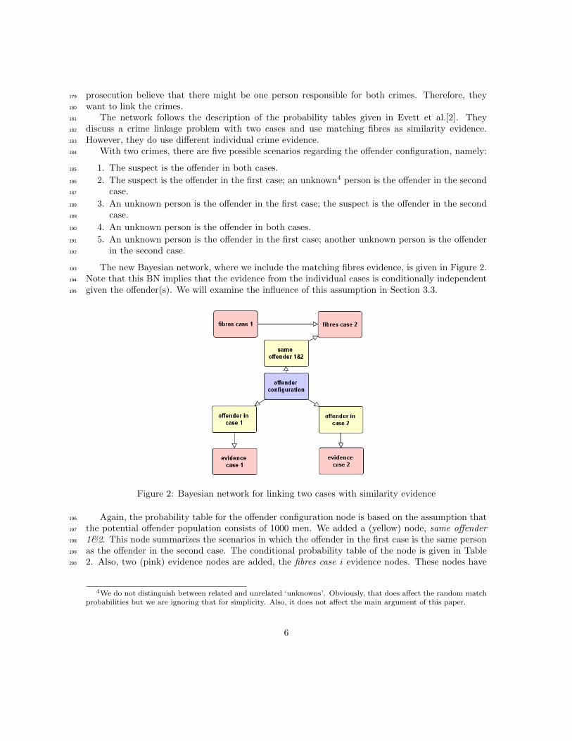
The new Bayesian network, where we include the matching fibres evidence, is given in Figure 2.193

Note that this BN implies that the evidence from the individual cases is conditionally independent194

given the offender(s). We will examine the influence of this assumption in Section 3.3.195

Figure 2: Bayesian network for linking two cases with similarity evidence

Again, the probability table for the offender configuration node is based on the assumption that196

the potential offender population consists of 1000 men. We added a (yellow) node, same offender197

1&2. This node summarizes the scenarios in which the offender in the first case is the same person198

as the offender in the second case. The conditional probability table of the node is given in Table199

2. Also, two (pink) evidence nodes are added, the fibres case i evidence nodes. These nodes have200

4We do not distinguish between related and unrelated ‘unknowns’. Obviously, that does affect the random matchprobabilities but we are ignoring that for simplicity. Also, it does not affect the main argument of this paper.

6

two states ‘type A’ (the type that is found on the crime scene and the balaclava) and ‘other’. To201

get the probability tables for these nodes, we need to determine how probable it is to observe fibres202

of type A. Suppose that the probability of observing this type of fibres in case 1 is 0.0001. We203

assume that if one person is responsible for both crimes, we will observe the same type of fibres in204

both cases.5 So, the probability tables are as in Table 3.205

same offender 1&2configuration both suspect suspect first suspect second same unknown different unknowns

Yes 1 0 0 1 0

No 0 1 1 0 1

Table 2: Probability table for the same offender 1&2 node

fibres case 1other 0.9999

type A 0.0001

fibres case 2same offender 1&2 no yes

fibres case 1 other type A other type A

other 0.9999 0.9999 1 0type A 0.0001 0.0001 0 1

Table 3: Probability tables for the fibres case i nodes

Now, by inserting the matching fibres evidence and the matching evidence from the individual206

cases 1 and 2, we can compute the posterior probabilities for the suspect being the offender. The207

probability that the suspect is the offender in case 1, given the evidence, has increased to 0.9999.208

In case 2, this posterior probability also increased to 0.9999. The probability that the suspect is209

the offender in both case 1 and case 2 follows from the offender configuration node. This posterior210

probability is 0.99988.211

The example shows that, by including evidence that increases the belief that the offenders in212

case 1 and 2 are the same, this also increases the belief that the suspect is the offender in the213

individual cases. The similarity evidence makes it possible that the value of evidence obtained214

in one case is ‘transferred’ to another case. The simple line of reasoning is as follows. There is215

evidence that the two crimes are committed by the same person. There is evidence that crime 1216

is committed by the suspect. The combination of these two pieces of evidence increases our belief217

that the suspect is the offender in crime 2, even without including the evidence found in crime 2.218

This also works the other way around, from crime 2 to crime 1.219

5In a more realistic setting, these numbers could be obtained by using a database of fibres. Also, other probabilitiesare involved, like the probability that the same balaclava was used by two different offenders. However, for thisexample the actual numbers are not that important, and we have chosen to follow the approach of Evett et al.[2].

7

Note that the likelihood ratio (LR), which is nowadays commonly reported by forensic experts,220

depends on the assumptions made about the prior probabilities of scenarios 1-5, see [16],[17]. This221

poses interesting reporting problems. However, this is not the main argument of this paper. In the222

following, we will focus on the posterior probabilities.223

It is important to note that the use of matching fibres as similarity evidence is provided just224

for convenience. As mentioned in Section 2.1, the distance between crime scenes, the time between225

crimes, the modus operandi or certain behaviour of the offender can provide very strong evidence226

that two crimes are committed by the same person. We could include any combination of these as227

similarity of crime evidence, but one can imagine that it is harder to come up with the probability228

for observing a certain modus operandi in a case. We could also include the work of Taroni[13] that229

concentrates on the question of the strength of the link between the cases.230

3.3. “Dependent” evidence231

In the last example, we assumed that the evidence obtained in the individual crimes is indepen-232

dent of each other, given the offender(s). However, if the pieces of evidence are of the same type233

(DNA, footmarks, eyewitness descriptions), knowing that the offender in both crimes is the same234

person makes them conditionally dependent. If one person is responsible for both burglaries, and235

we know that his DNA profile matches with the DNA profile obtained from the crime stain in case236

1, it is certain (ignoring all considerations of relevance and various types of errors) that his DNA237

profile will also match the crime stain in case 2. For our example, we will concentrate on a situation238

where the evidence in the individual cases consists of two pieces, one of a type that is also found in239

the other case and one of a ‘case individual’ type.240

In case 1, the evidence consists of a fingermark and a footmark of size 12. In case 2, the evidence241

consists of a partial DNA profile and a footmark of size 12. The suspect’s DNA profile matches242

with the partial DNA profile, his shoe size is 12 and his fingermark matches the fingermark from243

case 1. Clearly, the footmarks from the individual cases are conditionally dependent given whether244

or not the offender in both cases is the same person. We assume that shoes with size 12 have245

a population frequency of 0.01. The random match probability of the fingermark from case 1 is246

0.02. The random match probabilities of the partial DNA profile from case 2 is 0.03. Using these247

numbers, the combined evidential value of the evidential pieces in an individual case (which we248

assume to be conditionally independent) is the same as in the situations of Figure 1 and 2. The249

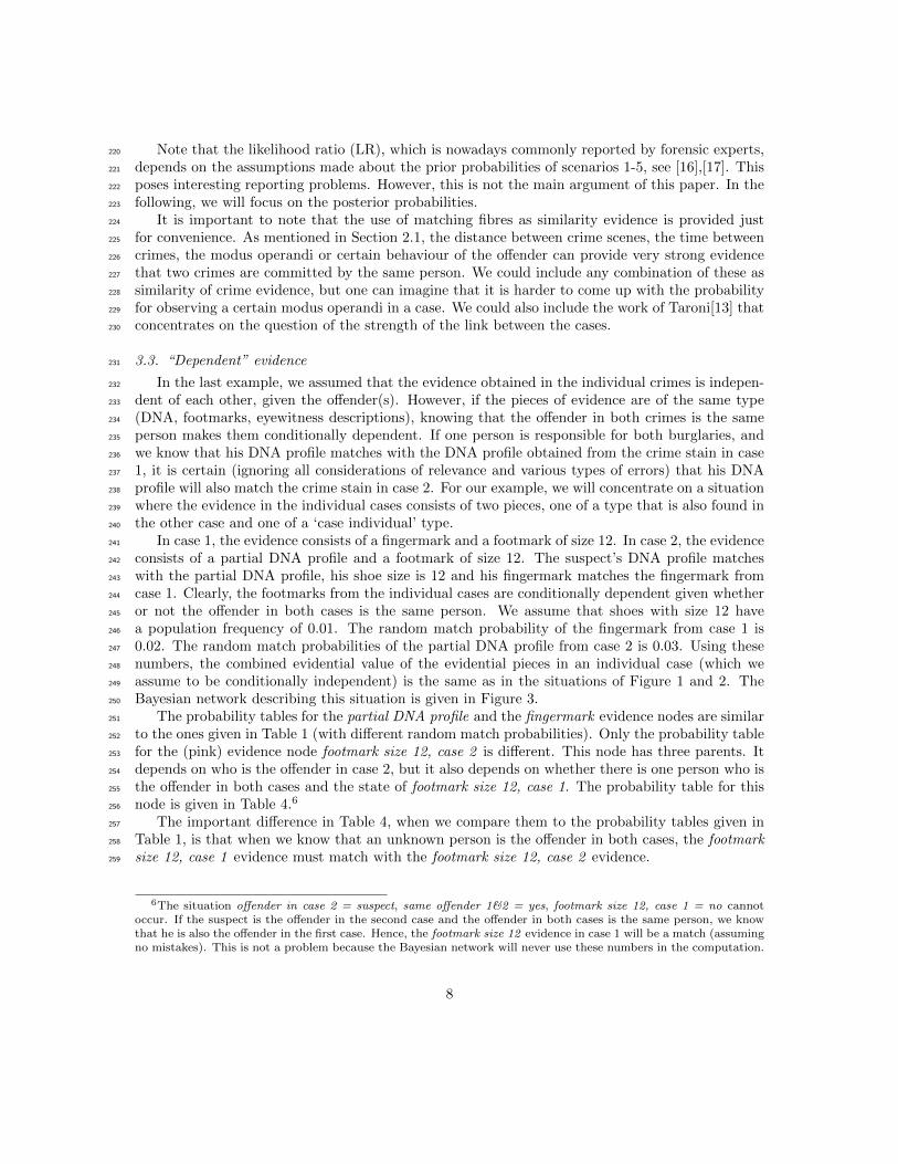
Bayesian network describing this situation is given in Figure 3.250

The probability tables for the partial DNA profile and the fingermark evidence nodes are similar251

to the ones given in Table 1 (with different random match probabilities). Only the probability table252

for the (pink) evidence node footmark size 12, case 2 is different. This node has three parents. It253

depends on who is the offender in case 2, but it also depends on whether there is one person who is254

the offender in both cases and the state of footmark size 12, case 1. The probability table for this255

node is given in Table 4.6256

The important difference in Table 4, when we compare them to the probability tables given in257

Table 1, is that when we know that an unknown person is the offender in both cases, the footmark258

size 12, case 1 evidence must match with the footmark size 12, case 2 evidence.259

6The situation offender in case 2 = suspect, same offender 1&2 = yes, footmark size 12, case 1 = no cannotoccur. If the suspect is the offender in the second case and the offender in both cases is the same person, we knowthat he is also the offender in the first case. Hence, the footmark size 12 evidence in case 1 will be a match (assumingno mistakes). This is not a problem because the Bayesian network will never use these numbers in the computation.

8

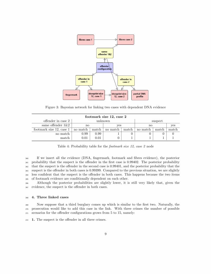
Figure 3: Bayesian network for linking two cases with dependent DNA evidence

footmark size 12, case 2offender in case 2 unknown suspect

same offender 1&2 no yes no yesfootmark size 12, case 1 no match match no match match no match match match

no match 0.99 0.99 1 0 0 0 0match 0.01 0.01 0 1 1 1 1

Table 4: Probability table for the footmark size 12, case 2 node

If we insert all the evidence (DNA, fingermark, footmark and fibres evidence), the posterior260

probability that the suspect is the offender in the first case is 0.99402. The posterior probability261

that the suspect is the offender in the second case is 0.99401, and the posterior probability that the262

suspect is the offender in both cases is 0.99399. Compared to the previous situation, we are slightly263

less confident that the suspect is the offender in both cases. This happens because the two items264

of footmark evidence are conditionally dependent on each other.265

Although the posterior probabilities are slightly lower, it is still very likely that, given the266

evidence, the suspect is the offender in both cases.267

4. Three linked cases268

Now suppose that a third burglary comes up which is similar to the first two. Naturally, the269

prosecution would like to add this case in the link. With three crimes the number of possible270

scenarios for the offender configurations grows from 5 to 15, namely:271

1. The suspect is the offender in all three crimes.272

9

2. The suspect is the offender in the first two crimes. An unknown person is the offender in the273

third crime.274

3. The suspect is the offender in the first and the third crime. An unknown person is the offender275

in the second crime.276

......277

14. An unknown person is the offender in the first crime. Another unknown person is the offender278

in the second and the third crime.279

15. Three different unknown persons are the offenders in the three crimes.280

In Appendix Appendix A we discuss the number of scenarios, given an arbitrary number, n, of281

cases.282

4.1. Assumptions about the evidence283

Again, the evidence in this case consists of footmark size 12. The same fibres as in case 1 and 2284

are found at the crime scene. The new same offender node summarises which cases have a common285

offender and has 5 states; (1) one offender for all cases, (2) one offender for the first two cases,286

another for the third, (3) one offender for the first and third case, another for the second, (4) one287

offender for the first case, another for the second and third and (5) three different offenders. The288

probability tables of the nodes fibre evidence case i are similar to those in Table 3 and are also289

based on the assumption that the fibre type occurs with probability 0.0001.290

The Bayesian network for this situation is given in Figure 4. The prior probabilities for the291

offender configuration have changed. Again we assume that the potential offender population292

consists of 1000 men. Under the assumption that each of these men is equally likely to be the offender293

in the individual cases, independently from each other we can compute the prior probabilities for294

all the scenarios. These are given in the fourth column of Table 5.295

If we insert the evidence, matching DNA profile, matching fingermark, footmarks of size 12 and296

matching fibres between the cases, we get the posterior probabilities for the offender configuration,297

given the evidence. These are given in the last column of Table 4. The distribution of posterior298

probabilities shows that it is very likely that the suspect is the offender in all cases (with probability299

0.99294). For the individual cases, the posterior probabilities that the suspect is the offender are300

0.99399, 0.99397 and 0.99299 respectively.301

4.2. Evidence proving innocence in the third case302

A piece of exculpatory evidence is found in the third case. In our example, an eyewitness303

description of the offender states that the offender has a permanent tattoo on his left arm. If the304

suspect does not have a tattoo on his left arm, and we assume that the eyewitness description is305

correct, i.e. the actual offender has a permanent tattoo, it is certain that the suspect is not the306

offender in the third case. Now, the prosecution can do two things, (1) drop the third case and go307

to court with the first two cases, where they have strong evidence of the suspect’s guilt, or (2) go308

to court with all three cases. The prosecution could argue that both options amount to the same309

outcome. In the first one, they drop the third case and use the evidence of the first two cases. In310

the second option, the prosecution uses all three but, since they have evidence that the suspect is311

innocent in the third crime, they are only interested in whether the suspect is guilty in the first two312

cases. We will show that the first option is wrong since it withholds exculpatory evidence from the313

court for the first two cases.314

10

Figure 4: Bayesian network for linking three cases with “dependent” evidence

When linking crimes, one needs to be aware that the sword cuts both ways. As we saw, if there315

is evidence in a case suggesting that there is one person responsible for both cases, evidence in one316

case is of interest for the question whether or not a suspect is guilty in another case. This means317

that if there is evidence in the first case that increases your belief that the suspect is the offender318

in the first case, it will also increase your belief that the suspect is the offender in the second case.319

This also works the other way around and is just as relevant: if there is evidence that a suspect is320

innocent in one case, this should also increase your belief that the suspect is innocent in the second321

case. This is illustrated by the example.322

Suppose that it is known that the proportion of men with a tattoo on their left arm is 1/25.7.323

The Bayesian network representing the situation is given in Figure 5. Remember that if we do not324

include the third case, we are in the situation of Figure 3.325

To compare the outcome in terms of the posterior probabilities when one drops or includes the326

third case, we compare the posterior probabilities of the offender configuration node of the models327

7In this case, where we insert as evidence that there is no match with the suspect, the probability is irrelevantsince it impossible to observe no match when the suspect is the donor (assuming no errors were made). In a situationwhere the evidence does not directly show that the suspect is innocent but where it only increases one’s belief thathe is innocent, the random match probability is relevant.

11

offender configuration

offender 1 offender 2 offender 3 prior probability posterior probabilityX X X 1.00 · 10−9 0.99X X 1 9.99 · 10−7 9.92 · 10−4

X 1 X 9.99 · 10−7 2.98 · 10−5

1 X X 9.99 · 10−7 1.98 · 10−5

X 1 1 9.99 · 10−7 2.98 · 10−5

X 1 2 9.97 · 10−4 2.97 · 10−6

1 X 1 9.99 · 10−7 1.98 · 10−5

1 X 2 9.97 · 10−4 1.98 · 10−6

1 1 X 9.99 · 10−7 5.95 · 10−7

1 2 X 9.97 · 10−4 5.94 · 10−8

1 1 1 9.99 · 10−7 5.95 · 10−3

1 1 2 9.97 · 10−4 5.94 · 10−6

1 2 1 9.97 · 10−4 5.94 · 10−6

2 1 1 9.97 · 10−4 5.94 · 10−6

1 2 3 0.99 5.92 · 10−7

Table 5: Prior and posterior probabilities for the offender configuration node, given that the offenderpopulation consists of 1000 men. The posterior probabilities are obtained by inserting the evidence.X represents the suspect, 1, 2 and 3 are other unknown men. The configuration 1, 2, X standsfor: An unknown man is the offender in the first case, another unknown man is the offender in thesecond case and the suspect is the offender in the third case.

.

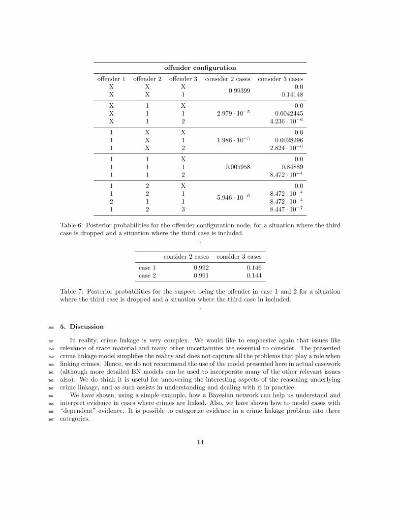
from Figure 3 and 5. This is done in Table 6. The posterior probabilities for the suspect being328

the offender in the individual cases under the situation where the third case is dropped and the329

situation where the third case is included are given in Table 7.330

The tables show that excluding or including the third case has serious consequences for the331

posterior probabilities, and thus, the outcome of a possible trial. When the third case is dropped,332

one can confidently state that it is very likely that the suspect is the offender in the first two cases.333

If we use the following two hypotheses,334

Hp: The suspect is the offender in case 1 and 2.335

Hd: The suspect is not the offender in case 1 nor in case 2.336

The posterior odds can be computed as

P(Hp|E)

P(Hd|E)=

0.99399

5.958 · 10−3 + 5.946 · 10−6= 167

The conclusion would be: Based on the observed evidence and the prior assumptions, it is 167 timesmore likely that the suspect is the offender in case 1 and 2 than that he is not the offender in case1 nor in case 2. When we include the third case and use the same hypothesis pair, the posteriorodds become,

P(Hp|E)

P(Hd|E)=

0.14148

0.84889 + 8.472 · 10−4 + 8.472 · 10−4 + 8.472 · 10−4 + 8.447 · 10−7= 0.17

12

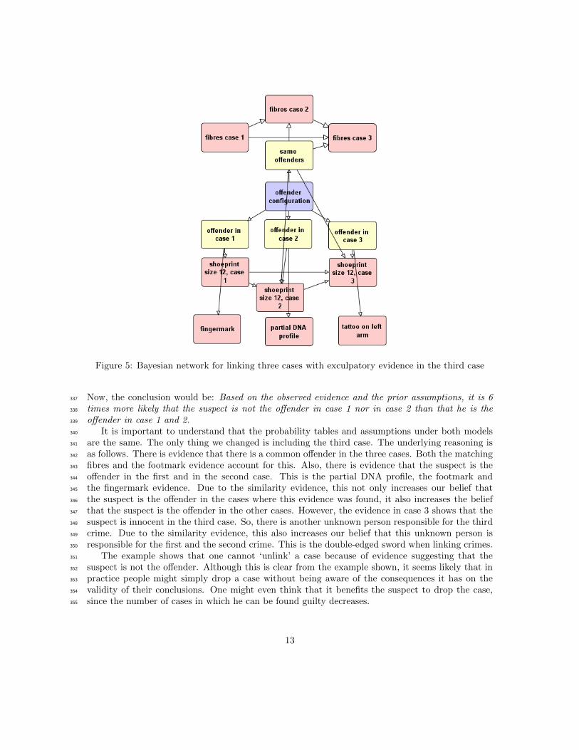
Figure 5: Bayesian network for linking three cases with exculpatory evidence in the third case

Now, the conclusion would be: Based on the observed evidence and the prior assumptions, it is 6337

times more likely that the suspect is not the offender in case 1 nor in case 2 than that he is the338

offender in case 1 and 2.339

It is important to understand that the probability tables and assumptions under both models340

are the same. The only thing we changed is including the third case. The underlying reasoning is341

as follows. There is evidence that there is a common offender in the three cases. Both the matching342

fibres and the footmark evidence account for this. Also, there is evidence that the suspect is the343

offender in the first and in the second case. This is the partial DNA profile, the footmark and344

the fingermark evidence. Due to the similarity evidence, this not only increases our belief that345

the suspect is the offender in the cases where this evidence was found, it also increases the belief346

that the suspect is the offender in the other cases. However, the evidence in case 3 shows that the347

suspect is innocent in the third case. So, there is another unknown person responsible for the third348

crime. Due to the similarity evidence, this also increases our belief that this unknown person is349

responsible for the first and the second crime. This is the double-edged sword when linking crimes.350

The example shows that one cannot ‘unlink’ a case because of evidence suggesting that the351

suspect is not the offender. Although this is clear from the example shown, it seems likely that in352

practice people might simply drop a case without being aware of the consequences it has on the353

validity of their conclusions. One might even think that it benefits the suspect to drop the case,354

since the number of cases in which he can be found guilty decreases.355

13

offender configuration

offender 1 offender 2 offender 3 consider 2 cases consider 3 casesX X X

0.993990.0

X X 1 0.14148

X 1 X2.979 · 10−5

0.0X 1 1 0.0042445X 1 2 4.236 · 10−6

1 X X1.986 · 10−5

0.01 X 1 0.00282961 X 2 2.824 · 10−6

1 1 X0.005958

0.01 1 1 0.848891 1 2 8.472 · 10−4

1 2 X

5.946 · 10−6

0.01 2 1 8.472 · 10−4

2 1 1 8.472 · 10−4

1 2 3 8.447 · 10−7

Table 6: Posterior probabilities for the offender configuration node, for a situation where the thirdcase is dropped and a situation where the third case is included.

.

consider 2 cases consider 3 cases

case 1 0.992 0.146case 2 0.991 0.144

Table 7: Posterior probabilities for the suspect being the offender in case 1 and 2 for a situationwhere the third case is dropped and a situation where the third case in included.

.

5. Discussion356

In reality, crime linkage is very complex. We would like to emphasize again that issues like357

relevance of trace material and many other uncertainties are essential to consider. The presented358

crime linkage model simplifies the reality and does not capture all the problems that play a role when359

linking crimes. Hence, we do not recommend the use of the model presented here in actual casework360

(although more detailed BN models can be used to incorporate many of the other relevant issues361

also). We do think it is useful for uncovering the interesting aspects of the reasoning underlying362

crime linkage, and as such assists in understanding and dealing with it in practice.363

We have shown, using a simple example, how a Bayesian network can help us understand and364

interpret evidence in cases where crimes are linked. Also, we have shown how to model cases with365

“dependent” evidence. It is possible to categorize evidence in a crime linkage problem into three366

categories.367

14

1. Evidence relevant for the question of who the offender is in a specific case.368

2. Evidence relevant for the question of whether the offender in two cases is the same person.369

3. A combination of 1 and 2: Evidence relevant for both questions.370

The first two categories are mentioned in Evett et al.[2]. The third category is a combination of371

the first two. For example if the similarity evidence is a match between fibres found at the different372

crime scenes, it falls in the second category. If, in addition, a sweater is found at the house of the373

suspect which fibres match with the fibres found at the crime scene, it belongs in the third category.374

When linking more than two crimes, the combined effect of different pieces of evidence, i.e. how375

one observation influences another, rapidly becomes more complex. The use of Bayesian networks376

helps us understand the relations between observations. In our example we have shown a model377

where three crimes are linked. Using a Bayesian network the problem breaks down to filling the378

entries of some very straightforward probability tables. We have only shown Bayesian networks for379

two and three crimes. In Appendix B Bayesian networks for situations with four and five crimes380

are presented.381

The number of possible offender configurations grows exponentially when the number of linked382

cases increases. Although we could use a computer to build a Bayesian network linking, e.g., twenty383

crimes and to fill the probability tables, the computation time will also increase according to the384

increase in offender configurations. The number of offender configurations with twenty crimes is385

474 869 816 156 751 [18]. When the number of linked crimes is not that high (say less than 10), the386

method to present and understand the relations between evidence described should help provide387

insight into the problem. For large numbers of linked crimes, further research needs to be done.388

More on this can be found in Appendix Appendix A and Appendix B.389

Most importantly, we have shown that one cannot ‘unlink’ cases. When there exists a link390

between cases, so there is evidence that there is one offender responsible for both cases, the cases391

should be treated simultaneously. In (forensic) practice, a similar thing occurs when multiple traces392

are secured of which the location of the traces suggest that they belong to one person, i.e. in a393

situation where fingermarks are recovered from an object. If these traces lay close to each other394

and form a grip pattern, it is likely that they belong to the same hand. Now, if only some of the395

fingermarks are similar to finger prints obtained from a suspect while the others are not, it is wrong396

to focus on the similarity evidence only.397

It would be interesting to see how judges and police investigators deal in practice with cases398

that appear to be linked, where evidence in one case points towards a suspect whereas in the other399

case the evidence suggests that the suspect is innocent. Our own limited experience is that the400

relevance of exculpatory evidence found in one case for other similar cases is underestimated. This401

hypothesis can be tested in properly designed experiments.402

Besides modelling linking of a large number of crimes, future research could study more complex403

situations of linked crimes. The research presented here could be expanded to situations where there404

is a group of criminals that e.g. rob houses together in various group compositions. In these cases it405

is possible to have a very similar and distinctive modus operandi, while the evidence in the different406

cases could point to different suspects.407

[1] F. Taroni, C. G. G. Aitken, P. Garbolino, and A. Biedermann. Bayesian Networks and Prob-408

abilistic Inference in Forensic Science. John Wiley & Sons, Ltd, Chichester, UK, February409

2006.410

[2] I. W. Evett, G. Jackson, D. V. Lindley, and D. Meuwly. Logical evaluation of evidence when a411

person is suspected of committing two separate offences. Science & Justice, 46(1):25–31, 2006.412

15

[3] O. Ribaux, A. Girod, S.J. Walsh, P. Margot, S. Mizrahi, and V. Clivaz. Forensic intelligence413

and crime analysis. Law and Psychology Review, pages 47–60, 2003.414

[4] J. Woodhams, R. Bull, and C.R Hollin. Case linkage: identifying crimes committed by the same415

offender. In Criminal Profiling: International Theory, Research and Practice, pages 117–133.416

Humana Press, 2007.417

[5] Crime linkage international network. Resource centre. http://www.birmingham.ac.uk/418

generic/c-link/activities/resources/index.aspx, 2014.419

[6] A. Davies. Rapists’ behaviour: a three aspect model as a basis for analysis and the identification420

of serial crime. Forensic Science International, 55(2):173–94, August 1992.421

[7] D. Grubin, P. Kelly, and C. Brunsdon. Linking Serious Sexual Assaults Through Behaviour.422

Technical report, Home Office - Research, Development and Statistics Directorate, 2001.423

[8] R. R. Hazelwood and J. I. Warren. Linkage analysis: Modus operandi, ritual, and signature424

in serial sexual crime. Aggression and Violent Behavior, 8(6):587–598, November 2003.425

[9] W. Petherick. Profiling and Serial Crime - Theoretical and practical issues. Anderson, 3rd426

edition, 2014.427

[10] C. Bennell and D. V. Canter. Linking commercial burglaries by modus operandi: tests using428

regression and ROC analysis. Science & Justice, 42(3):153–64, 2002.429

[11] M. Tonkin, J. Woodhams, R. Bull, and J. W. Bond. Behavioural case linkage with solved and430

unsolved crimes. Forensic Science International, 222(1-3):146–53, October 2012.431

[12] F. Taroni. Serial crime : a consideration of investigative problems. Forensic Science Interna-432

tional, 65:33–45, 1994.433

[13] F. Taroni, S. Bozza, and A. Biedermann. Two items of evidence, no putative source: an infer-434

ence problem in forensic intelligence. Journal of Forensic Sciences, 51(6):1350–61, November435

2006.436

[14] N. Fenton, M. Neil, and A. Hsu. Calculating and understanding the value of any type of match437

evidence when there are potential testing errors. Artificial Intelligence and Law, 22(1):1–28,438

October 2014.439

[15] I. W. Evett, P. D. Gill, G. Jackson, J. Whitaker, and C. Champod. Interpreting small quantities440

of DNA: the hierarchy of propositions and the use of Bayesian networks. Journal of Forensic441

Sciences, 47(3):520–30, May 2002.442

[16] J. S. Buckleton, C. M. Triggs, and C. Champod. An extended likelihood ratio framework for443

interpreting evidence. Science & Justice, 46(2):69–78, 2006.444

[17] F. Taroni and A. Biedermann. Inadequacies of posterior probabilities for the assessment of445

scientific evidence. Law, Probability and Risk, 4(1-2):89–114, March 2005.446

[18] OEIS Foundation Inc. The on-line encyclopedia of integer sequences. http://oeis.org/447

A000110, 2014.448

16

Funding449

This work was supported by the Netherlands Organisation for Scientific Research (NWO) as450

part of the project “Combining Evidence” in the Forensic Science programme [727.011.007].451

17

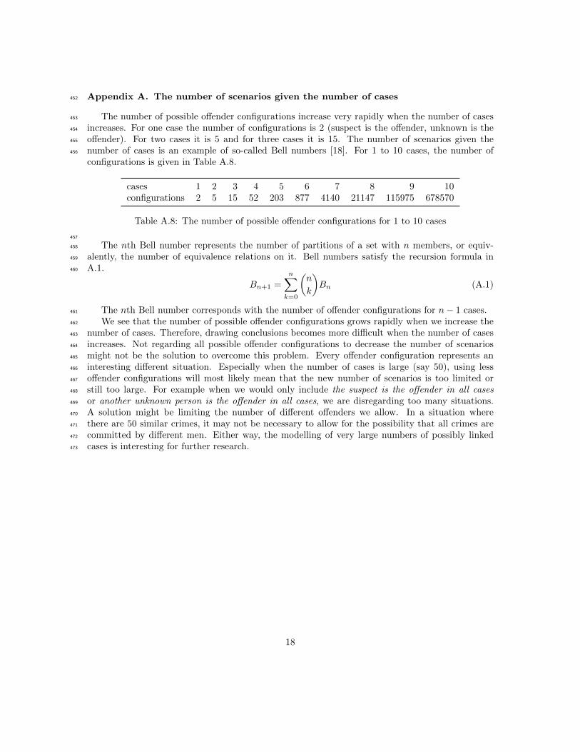
Appendix A. The number of scenarios given the number of cases452

The number of possible offender configurations increase very rapidly when the number of cases453

increases. For one case the number of configurations is 2 (suspect is the offender, unknown is the454

offender). For two cases it is 5 and for three cases it is 15. The number of scenarios given the455

number of cases is an example of so-called Bell numbers [18]. For 1 to 10 cases, the number of456

configurations is given in Table A.8.

cases 1 2 3 4 5 6 7 8 9 10configurations 2 5 15 52 203 877 4140 21147 115975 678570

Table A.8: The number of possible offender configurations for 1 to 10 cases

457

The nth Bell number represents the number of partitions of a set with n members, or equiv-458

alently, the number of equivalence relations on it. Bell numbers satisfy the recursion formula in459

A.1.460

Bn+1 =

n∑k=0

(n

k

)Bn (A.1)

The nth Bell number corresponds with the number of offender configurations for n− 1 cases.461

We see that the number of possible offender configurations grows rapidly when we increase the462

number of cases. Therefore, drawing conclusions becomes more difficult when the number of cases463

increases. Not regarding all possible offender configurations to decrease the number of scenarios464

might not be the solution to overcome this problem. Every offender configuration represents an465

interesting different situation. Especially when the number of cases is large (say 50), using less466

offender configurations will most likely mean that the new number of scenarios is too limited or467

still too large. For example when we would only include the suspect is the offender in all cases468

or another unknown person is the offender in all cases, we are disregarding too many situations.469

A solution might be limiting the number of different offenders we allow. In a situation where470

there are 50 similar crimes, it may not be necessary to allow for the possibility that all crimes are471

committed by different men. Either way, the modelling of very large numbers of possibly linked472

cases is interesting for further research.473

18

Appendix B. Bayesian networks for more cases474

In this section we present Networks for situations with four and five cases. As can be seen475

from Table A.8, the number of possible offender configurations is 52 for four cases and 203 for five476

cases. The probability tables are straightforward, and could therefore be made by the computer.477

We included an extra node. One that represents the number of men in the potential offender478

population. This node gives us the possibility to examine the influence of the prior on the posterior479

probabilities. The Bayesian networks in Figure B.6 and B.7 are similar to the networks we saw480

before and show that it is possible to use the same methods to model situations with more cases.481

Figure B.6: A Bayesian network linking four cases where the evidence consists of partial, overlap-ping, DNA profiles

19

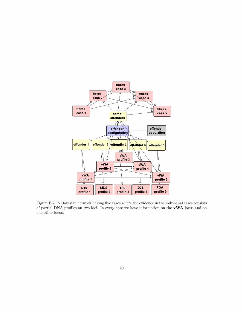
Figure B.7: A Bayesian network linking five cases where the evidence in the individual cases consistsof partial DNA profiles on two loci. In every case we have information on the vWA locus and onone other locus.

20