Modelling breakup process of a liquid drop in shear flow

Available online at www.sciencedirect.com

Applied Mathematical Modelling 33 (2009) 315–328

www.elsevier.com/locate/apm

Modelling breakup process of a liquid drop in shear flow

A. Fasano, F. Rosso *

Dip. Matematica Ulisse Dini, Universita di Firenze, Viale Morgagni 67/a, 50134 Firenze, Italy

Received 21 November 2006; received in revised form 25 October 2007; accepted 5 November 2007Available online 22 November 2007

Abstract

The aim of this paper is to give a contribution within the mathematical modelling of the deformation and breakup of adroplet in a continuous immiscible liquid phase in impulsively started shear flow. Starting from the results of Cristini et al.[V. Cristini, S. Guido, A. Alfani, J. Blawzdziewicz, M. Loewenberg, Drop breakup and fragment distribution in shear flow,J. Rheol. 47 (5) (2003) 1283–1298] we extrapolate a general scheme for the whole breakage process, on the basis of whichwe formulate a procedure for the computation of the size distribution function at the end of the process.� 2007 Elsevier Inc. All rights reserved.

Keywords: Drop size distribution; Breakage processes; Liquid–liquid dispersions; Multiple breakage

1. Introduction

The literature concerning the evolution of liquid–liquid dispersions is extremely large, testifying the impor-tance of the subject both from the industrial and the theoretical point of view. In a recent paper [1] we haveoutlined the state of the art about the breakage and coalescence kernels proposed by several authors and theprogress in mathematical modelling including the so-called volume scattering effect and the influence of multi-ple breakage. We refer to [1] for the relevant references.

The deformation and breakup of a droplet in a continuous immiscible liquid phase under microconfined flow isa subject of growing interest in several applications. Examples are microfluidics technologies and emulsion pro-cessing (see for example [2]). However, the current understanding of drop deformation, even in well-controlledflow fields, is rather limited, and the design issues concerning drop rheological behavior in microdevices are oftenaddressed on an empirical basis. Significant advances in modelling coagulation–fragmentation processes inmicrodevices can be found in a series of papers [3–6,4,7–10]. In particular [6] refers to the stochastic breakupin a turbulent flow, while the other papers are related to the case of laminar shear flow. The resulting theory israther comprehensive, since it proceeds on physical bases and includes the computational aspects.

In order to be specific, in the present paper we make explicit reference to the paper [3] by Cristini et al. con-cerning the study of the phenomenon of deformation and breakup of drops in impulsively started shear flow.

0307-904X/$ - see front matter � 2007 Elsevier Inc. All rights reserved.

doi:10.1016/j.apm.2007.11.006

* Corresponding author.E-mail addresses: [email protected] (A. Fasano), [email protected] (F. Rosso).

mailto:[email protected]

mailto:[email protected]

316 A. Fasano, F. Rosso / Applied Mathematical Modelling 33 (2009) 315–328

The advantage of the setting of such research is that breakage is isolated from the other phenomena usuallytaking place in liquid–liquid dispersions and it occurs in well known and well reproducible conditions. Whenshear is applied a drop is transformed in an elongated body which undergoes a sequence of breakage events.

The sequence of Figs. 1–5, show the various phases of the breakup of a single mother drop and are takenfrom a real experiment (courtesy of S. Guido).

In [3], the authors summarize their results in a simplified model providing the clue that the size distributionof the produced droplets seems to scale with the critical size drop for breakage. From their calculations weextrapolate a general scheme for the whole breakage process, on the basis of which we can formulate a pro-cedure for the computation of the size distribution function at the end of the process. In our scheme weemphasize the fact that each breakage sequence leaves a residual drop, whose contribution to the final distri-bution may not be negligible if the average number of breakage events in a sequence is not large. For instancewe can say that if that average is about 10, the cumulative volume of the residual drops is of the order of 10%of the total volume of the dispersed phase.

Clearly, the calculation of the distribution size of the residual drops is not simple, since their size dependson the specific sequence that has generated it.

In what follows we illustrate the formal steps for the derivation of the distribution function following abreakage experiment, including the influence of residual drops.

The intent of this study is mainly theoretical, since residual drops are not going to alter the final size dis-tribution to a significant extent when most of the drops decay in a large number of daughters. However,besides the importance of producing a nicely self-consistent theory, a practical relevance can be found when

Fig. 1. A drop starts to elongate in a plane shear flow.

Fig. 2. Maximum elongation is reached and breakage starts.

Fig. 3. Primary breakage event. Primary drops, satellites and residual body are clearly visible.

Fig. 4. An ordinary breakage event of the elongated body.

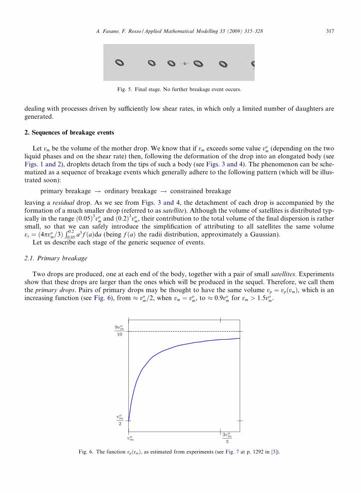
Fig. 5. Final stage. No further breakage event occurs.

A. Fasano, F. Rosso / Applied Mathematical Modelling 33 (2009) 315–328 317

dealing with processes driven by sufficiently low shear rates, in which only a limited number of daughters aregenerated.

2. Sequences of breakage events

Let vm be the volume of the mother drop. We know that if vm exceeds some value vom (depending on the two

liquid phases and on the shear rate) then, following the deformation of the drop into an elongated body (seeFigs. 1 and 2), droplets detach from the tips of such a body (see Figs. 3 and 4). The phenomenon can be sche-matized as a sequence of breakage events which generally adhere to the following pattern (which will be illus-trated soon):

primary breakage ! ordinary breakage ! constrained breakage

leaving a residual drop. As we see from Figs. 3 and 4, the detachment of each drop is accompanied by theformation of a much smaller drop (referred to as satellite). Although the volume of satellites is distributed typ-ically in the range ð0:05Þ3vo

m and ð0:2Þ3vom, their contribution to the total volume of the final dispersion is rather

small, so that we can safely introduce the simplification of attributing to all satellites the same volumevs ¼ ð4pvo

m=3ÞR 0:2

0:05a3f ðaÞda (being f ðaÞ the radii distribution, approximately a Gaussian).

Let us describe each stage of the generic sequence of events.

2.1. Primary breakage

Two drops are produced, one at each end of the body, together with a pair of small satellites. Experimentsshow that these drops are larger than the ones which will be produced in the sequel. Therefore, we call themthe primary drops. Pairs of primary drops may be thought to have the same volume vp ¼ vpðvmÞ, which is anincreasing function (see Fig. 6), from � vo

m=2, when vm ¼ vom, to � 0:9vo

m for vm > 1:5vom.

Fig. 6. The function vpðvmÞ, as estimated from experiments (see Fig. 7 at p. 1292 in [3]).


Some of the breakage processes may consist just in the formation of the principal drops, plus an unbreak-able residue. The conditions for this event will be discussed in the following subsection. Here we point out that,even in this special event, for simplicity of exposition we always associate to primary breakage the productionof two satellites, so that the minimal volume of a primary droplet is vo

m=2� vs. Due to the smallness of the ratiovs=vo

m � 10�3 and to uncertainty of the value of vom, such a simplification is irrelevant.

2.2. Ordinary breakage

Each breakage event reduces the volume vb of the elongated body by producing a pair of daughter dropletsðv1; v2Þ and a pair of satellites. In an ordinary breakage event vb is large enough to allow both volumes v1; v2 totake values in the admissible range ðvmin; vmaxÞ. Typically vmax � 2vmin. Daughters volumes have a distributionfunction F ðvÞ supported in ðvmin; vmaxÞ. The condition on vb guaranteeing an ordinary breakage event is

vb > 2ðvmax þ vsÞ: ð1Þ
In the sequel it will be convenient to look at ðv1; v2Þ as an ordered pair vmin 6 v1 6 v2 6 vmax. It is easy to get anestimate of the maximum and of the minimum number of ordinary events. After the separation of the primarydroplets the volume of the elongated body is
vð1Þb ¼ vm � 2vp � 2vs:

The maximum number Nmax of ordinary events corresponds to the hypothetical situation in which the daugh-ters in all events have the minimum volume:

0 < vð1Þb � 2Nmaxðvmin þ vsÞ < 2ðvmax þ vsÞ;
the latter inequality preventing a further ordinary breakage. Thus
vð1Þb

2ðvmin þ vsÞ� vmax þ vs

vmin þ vs< N max <

vð1Þb

2ðvmin þ vsÞ: ð2Þ

Since vmax ’ 2vmin we have

vmax þ vs

vmin þ vs’ 2� vs

vmin

;

so that Nmax can be, at most, one unit less than the maximum integer in vð1Þb =ð2ðvmin þ vsÞÞ. Similarly Nmin isdefined by the inequalities

0 < vð1Þb � 2Nminðvmax þ vsÞ < 2ðvmax þ vsÞ
implying
N min ¼vð1Þb

2ðvmax þ vsÞ

" #; ð3Þ

½�� denoting the maximum integer.Clearly the actual number N of ordinary events in a sequence depends on the outcome of each event of the

sequence. If in the jth event the cumulative volume of the daughters is 2V ðjÞ, then the sequence of ordinaryevents will be terminated when

vð1Þb �XN

j¼1

2ðV ðjÞ þ vsÞ < 2ðvmax þ vsÞ; ð4Þ

which defines N implicitly. Of course N ¼ 0 if vð1Þb < 2ðvmax þ vsÞ.

2.3. Constrained breakage

The l.h.s. of (4) defines the volume of the elongated body after the N þ 1 events, including the one produc-ing the primary drops:

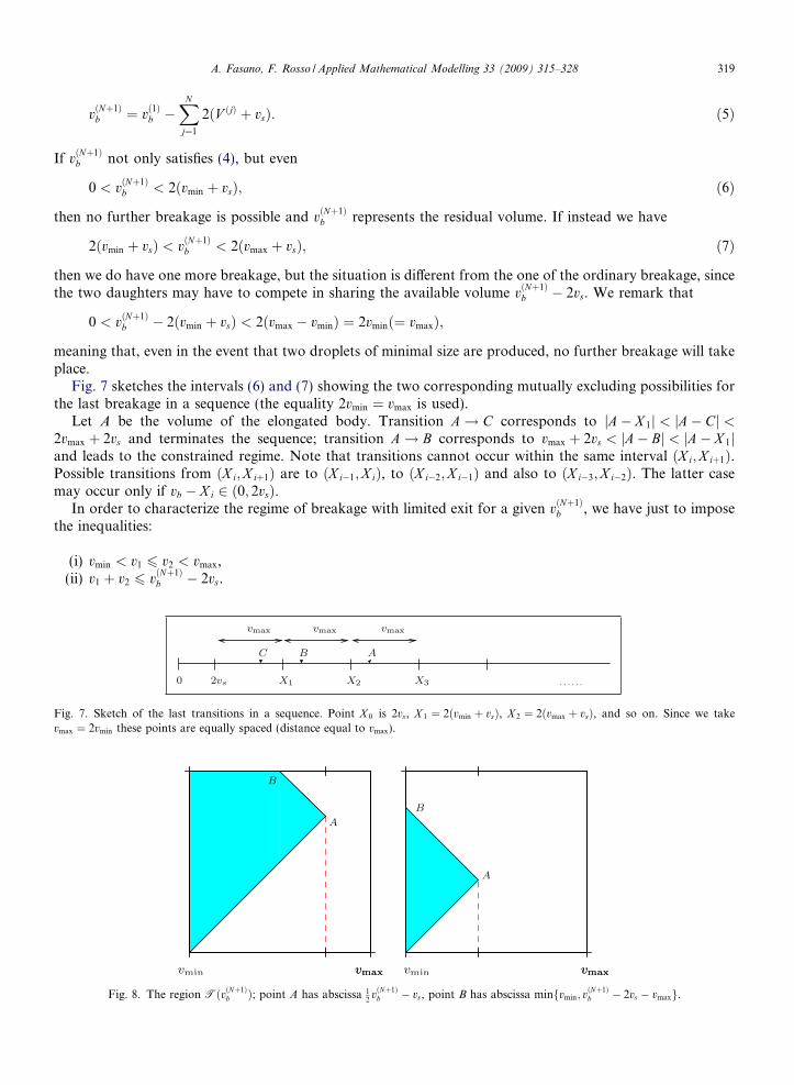
Fig. 7vmax ¼


vðNþ1Þb ¼ vð1Þb �

XN

j¼1

2ðV ðjÞ þ vsÞ: ð5Þ

If vðNþ1Þb not only satisfies (4), but even

0 < vðNþ1Þb < 2ðvmin þ vsÞ; ð6Þ

then no further breakage is possible and vðNþ1Þb represents the residual volume. If instead we have

2ðvmin þ vsÞ < vðNþ1Þb < 2ðvmax þ vsÞ; ð7Þ

then we do have one more breakage, but the situation is different from the one of the ordinary breakage, sincethe two daughters may have to compete in sharing the available volume vðNþ1Þ

b � 2vs. We remark that

0 < vðNþ1Þb � 2ðvmin þ vsÞ < 2ðvmax � vminÞ ¼ 2vminð¼ vmaxÞ;

meaning that, even in the event that two droplets of minimal size are produced, no further breakage will takeplace.

Fig. 7 sketches the intervals (6) and (7) showing the two corresponding mutually excluding possibilities forthe last breakage in a sequence (the equality 2vmin ¼ vmax is used).

Let A be the volume of the elongated body. Transition A! C corresponds to jA� X 1j < jA� Cj <2vmax þ 2vs and terminates the sequence; transition A! B corresponds to vmax þ 2vs < jA� Bj < jA� X 1jand leads to the constrained regime. Note that transitions cannot occur within the same interval ðX i;X iþ1Þ.Possible transitions from ðX i;X iþ1Þ are to ðX i�1;X iÞ, to ðX i�2;X i�1Þ and also to ðX i�3;X i�2Þ. The latter casemay occur only if vb � X i 2 ð0; 2vsÞ.

In order to characterize the regime of breakage with limited exit for a given vðNþ1Þb , we have just to impose

the inequalities:

(i) vmin < v1 6 v2 < vmax,(ii) v1 þ v2 6 vðNþ1Þ

b � 2vs.

. Sketch of the last transitions in a sequence. Point X 0 is 2vs, X 1 ¼ 2ðvmin þ vsÞ, X 2 ¼ 2ðvmax þ vsÞ, and so on. Since we take2vmin these points are equally spaced (distance equal to vmax).

Fig. 8. The region TðvðNþ1Þb Þ; point A has abscissa 1

2vðNþ1Þ

b � vs, point B has abscissa minfvmin; vðNþ1Þb � 2vs � vmaxg.


Thus the pair ðv1; v2Þ belongs to the domain TðvðNþ1Þb Þ shown in Fig. 8 corresponding to sup v1 ¼

ð1=2ÞvðNþ1Þb � vs larger (case (a)) or smaller (case (b)) than the mean v ¼ ðvmin þ vmaxÞ=2.

The segment AB is found taking the equality sign in (ii) above and corresponds to the ideal situation inwhich no residual drop is left. Clearly the maximal residual drop is obtained in the opposite ideal casev1 ¼ v2 ¼ vmin, leaving vmax

res ¼ vðNþ1Þb � 2ðvs þ vminÞ. According to inequalities (7), the latter quantity belongs

to ð0; vmaxÞ, as we have already seen.

2.4. The residual drop

The volume of the residual drop vres < 2ðvmin þ vsÞ depends on the volume of the mother drop and on thewhole sequence of events. We remark that the range of vres encompasses the whole volume range of daughterdroplets. We have the following cases:

(a) No breakage: vres ¼ vm if vm < vom, i.e. the distribution function of the mother drops is not altered below

vom.

(b) Primary breakage only: vres ¼ vð1Þb if 0 < vð1Þb < 2ðvmin þ vsÞ, i.e. 2ðvp þ vsÞ < vm < 2ðvp þ vmin þ 2vsÞ.(c) Primary breakage followed by a breakage sequence not including constrained breakage: vres ¼ vðNþ1Þ

b .(d) Breakage sequence terminating with constrained breakage: vres ¼ vðNþ2Þ

b .

3. The final distribution

3.1. Contribution of primary breakage

As we said, the primary breakage either is not possible, or it occurs with probability one. Among the pri-mary droplets we have to distinguish those having the maximum volume vp � 0:9vo

m from the smaller ones. IfwðvmÞ is the distribution of the mother droplets, the number of drops with volume 0:9vo

m produced by primarybreakage is

nmaxp ¼ 2

Z V o

1:5vom

wðvmÞdvm; ð8Þ

where V o is the upper bound of the support of wðvmÞ.Considering smaller drops, the number of primary drops with volume between vp and vp þ dvp will be

2wðvmÞdvm, with dvm ¼ dvp=v0pðvmÞ. Thus the distribution function of the primary drops for vp < 0:9vom is

uprmðvpÞ ¼ 2wð~vmÞv0pð~vmÞ

;1

2vo

m < vp < 0:9vom; ð9Þ

where ~vmðvpÞ is the inverse function of vpðvmÞ.

3.2. Contribution of ordinary breakage

Let us now consider the sequence of ordinary breakage events. Each event consists in the separation of adaughter (and a satellite) from each side of the elongated body (see Figs. 1–5). The two processes can be con-sidered independent of each other. If F ðvÞdv is the probability that a daughter drop has volume in the intervalðv; vþ dvÞ (with

R vmax

vminF ðvÞdv ¼ 1) then the probability for a pair of drops to fall in the element

ðv1; v1 þ dv1Þ � ðv2; v2 þ dv2Þ is F ðv1ÞF ðv2Þdv1 dv2, if we disregard for the moment the size ordering and we justthink of the pair as the outcome of an experiment repeated twice. However, we are not interested in which ofthe drops is ‘‘first” or ‘‘second” (or, equally, ‘‘ left” or ‘‘right”); thus the probability density for a pair ðv1; v2Þ,which we may order just by size, is 2F ðv1ÞF ðv2Þ. The integral over the square ðvmin; vmaxÞ � ðvmin; vmaxÞ of theproduct F ðv1ÞF ðv2Þ is 1, as well as the integral of 2F ðv1ÞF ðv2Þ over the triangle T ¼ fvmin < v1 < v2 < vmaxg.

If we allow F to depend on the volume of the elongated body we would be forced to update F after eachbreakage event. It looks natural to suppose that the elongated body keeps no memory of the original volume


vm of the mother drop. Instead, it seems more realistic to assume that F remains the same for all ordinaryevents and is affected by the size of the elongated body only when the regime of breakage with limited exitsis entered.

Accordingly, we claim that, for any v� 2 ðvmin; vmaxÞ, the number of daughters with volume in ðv�; v� þ dv�Þproduced by any of the mother drops in a sequence of N ordinary events is

Fig. 9.lying i

uðNÞordðv�Þdv� ¼ F ðv�Þdv � 2NZ V o

v1m

P ðN ; vmÞwðvmÞdvm ð10Þ

being v1m ¼ 2ðvp þ 2vs þ vminÞ and P ðN ; vmÞ the probability (still to be found) that a drop of volume vm can gen-

erate a sequence of exactly N ordinary events. In order to compute the latter, suppose we know that in eachordinary event the probability that the produced pair ðv1; v2Þ has cumulative volume v1 þ v2 between 2V and2ðV þ dV Þ is pðV ÞdV (with

R vmax

vminpðV ÞdV ¼ 1). Then take an ordered sequence vmin 6 V ð1Þ 6

V ð2Þ 6 . . . 6 V ðNÞ < vmax such that inequality (4) is satisfied for a given vm (this is a further condition on N

which is between NminðvmÞ and N maxðvmÞ). The set SðvmÞ of all such sequences defines a domain SðvmÞ inthe N max-dimensional cube with side ðvmin; vmaxÞ. We denote by SN ðvmÞ the set of all sequences with N ele-ments, defining the N-dimensional subdomain SN ðvmÞ. Then we can say that

P ðN ; vmÞ ¼ N !

ZSN ðvmÞ

pðV ð1ÞÞpðV ð2ÞÞ � � � pðV ðNÞÞdV ð1ÞdV ð1Þ � � � dV ðNÞ: ð11Þ

We denote by NðvmÞ the set of all possible values of N in SðvmÞ, i.e. the integers between NminðvminÞ andNmaxðvminÞ. So we can express the contribution of ordinary events to the resulting distribution of daughters’volume as

uordðv�Þ ¼ 2F ðv�ÞZ V o

v1m

XN2NðvmÞ

NP ðN ; vmÞwðvmÞdvm: ð12Þ

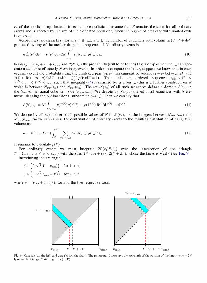
It remains to calculate pðV Þ.For ordinary events we must integrate 2F ðv1ÞF ðv2Þ over the intersection of the triangle

T ¼ fvmin < v1 6 v2 < vmaxg with the strip 2V < v1 þ v2 < 2ðV þ dV Þ, whose thickness isffiffiffi2p

dV (see Fig. 9).Introducing the arclength

n 2 0;ffiffiffi2pðV � vminÞ

� �for V < v;

n 2 0;ffiffiffi2pðvmax � V Þ

� �for V > v;

where v ¼ ðvmin þ vmaxÞ=2, we find the two respective cases

Case (a) (on the left) and case (b) (on the right). The parameter n measures the arclength of the portion of the line v1 þ v2 ¼ 2Vn the triangle T starting from ðV ; V Þ.


2

Z ffiffi2pðV�vminÞ

0

F V � nffiffiffi2p

� �F V þ nffiffiffi

2p

� �dn �

ffiffiffi2p

dV ðcase ðaÞÞ;

2

Z ffiffi2pðvmax�V Þ

0

F V � nffiffiffi2p

� �F V þ nffiffiffi

2p

� �dn �

ffiffiffi2p

dV ðcase ðbÞÞ:ð13Þ

Returning to the variable v1 ¼ V � n=ffiffiffi2p

we arrive at the final formula

pðV Þ ¼ 4

Z V

IðV ÞF ðv1ÞF ð2V � v1Þdv1 ð14Þ

with

IðV Þ ¼ vmin for V 2 vmin;vmin þ vmax

2

� �;

IðV Þ ¼ 2V � vmax for V 2 vmin þ vmax

2; vmax

� �:

ð15Þ

Remark 1. The function pðV Þ is indeed a probability density, i.e.R vmax

vminpðV ÞdV ¼ 1. This can be checked easily

since the latter integral, recalling (13), is twice the integral of the product F ðv1ÞF ðv2Þ over the trianglevmin < v1 6 v2 < vmax which in turn equals the product

R vmax

vminF ðv1Þdv1

R vmax

vminF ðv2Þdv2 ¼ 1. Similarly we can

check that pðV Þ provides the correct value of daughter droplets volume hvi ¼R vmax

vminvF ðvÞdv:
Z vmax
vmin

2VpðV ÞdV ¼Z vmax

vmin

Z vmax

vmin

ðv1 þ v2ÞF ðv1ÞF ðv2Þdv1 dv2

¼Z vmax

vmin

Z vmax

vmin

v1F ðv1Þdv1

� �F ðv2Þdv2 þ

Z vmax

vmin

Z vmax

vmin

v2F ðv2Þdv2

� �F ðv1Þdv1 ¼ 2hvi:

3.3. Contribution of the residual drops

The last step needed to determine the final volume distribution function is the evaluation of the contribu-tion uresðv�Þ of residual drops. According to our description in Section 2.4, ures is the sum of the followingterms:

(a) The unaltered tail of the original distribution function wðv�Þ
uaðv�Þ ¼ wðv�Þ with v� 2 ð0; 2vp þ 2vsÞ: ð16Þ
(b) The contribution coming directly from primary breakage, namely

ubðv�Þ ¼ 2wðv� þ 2vp þ 2vsÞ with v� 2 ð0; 2vmin þ 2vsÞ: ð17Þ
(c) The sum over N of the contribution due to all sequences of order N having a residual drop v� after ordin-
ary events only.(d) The sum over N of the contribution due to all sequences ending with a constrained breakage event with

residual volume v�.

Also in cases (c), (d) we select v� 2 ð0; 2vmin þ 2vsÞ. Computing ucðv�Þ;udðv�Þ is not trivial. Let us calculateuc. We note that a given residual volume v� can be obtained after N ordinary breakage events only if the fol-lowing conditions are satisfied:

(i) vm belongs to the interval

Iðv�;NÞ ¼ f2vp þ 2ðN þ 1Þvs þ 2Nvmin þ v� < vm

< 2vp þ 2ðN þ 1Þvs þ 2Nvmax þ v�g\ðv1

m; V0Þ;

(we recall that v1m ¼ 2ðvp þ 2vs þ vminÞ).


(ii) For a given vm satisfying (i) above, the sequence V ð1Þ; . . . ; V ðNÞ belongs to a suitable subsetcSN ðvm; v�Þ �SN ðvmÞ, corresponding to a subdomain
bSN ðvm; v�Þ � SN ðvmÞ
having one dimension less than SN . Indeed bSN ðvm; v�Þ is the intersection of SN ðvmÞ with the hyperplane

vð1Þb �XN

j¼1

2ðV ðjÞ þ vsÞ ¼ v�: ð18Þ

We remark that SN is the union of two disjoint sets:

SN ¼ Sð0ÞN [S

ð‘ÞN ;

where Sð0ÞN is defined through inequality (6) and S

ð‘ÞN through inequalities (7). Thus S

ð0ÞN is the set of

sequences consisting only of ordinary events, while Sð‘ÞN is the set of sequences ending with a breakage

with limited exit. Clearly cSN is a subset of Sð0ÞN , because of limitation v� 2 ð0; 2vmin þ 2vsÞ.

(iii) Only those values of N can be used for which the interval Iðv�;NÞ is not empty. Indeed N has to be lessthan N ð0Þ defined as

N ð0Þðv�Þ ¼ supNf2vp þ 2ðN þ 1Þvs þ 2Nvmin < V 0 � v�g: ð19Þ

To clarify our exposition, let us specialize the procedure for the first four possible values of N. For N ¼ 1,since vm ¼ v� þ 2vp þ 4vs þ 2V ð1Þ, we have 2vp þ 4vs þ 2vmin 6 vm � v� 6 2vp þ 4vs þ 2vmax, which definesIðv�; 1Þ. The subset cS1ðvm; v�Þ consists of a single event with V ð1Þ ¼ 1

2ðvm � v�Þ � vp � 2vs and the subdomainbS 1ðvm; v�Þ reduces to a point. Thus the contribution to uc is

uð1Þc ðv�Þ ¼Z

Iðv�;1Þp

1

2ðvm � v�Þ � vp � 2vs

� �wðvmÞdvm:

For N ¼ 2, vm ¼ v� þ 2vp þ 6vs þ 2ðV ð1Þ þ V ð2ÞÞ, implying the definition of Iðv�; 2Þ.Among the sequences in S2ðvmÞ we must select those satisfying

V ð1Þ þ V ð2Þ ¼ 1

2ðvm � v�Þ � vp � 3vs ¼ 2V ; V 2 ðvmin; vmaxÞ; ð20Þ

thus the subdomain bS 2ðvm; v�Þ is one-dimensional.The number of residual drops produced with volume in the interval ðv�; v� þ dv�Þ is obtained by integrating

over the interval Iðv�; 2Þ the original distribution wðvmÞ multiplied by the integral of 2pðV ð1ÞÞpðV ð2ÞÞ over theinfinitesimal strip between the lines bS 2ðvm; v�Þ; bS2ðvm; v� þ dv�Þ. The latter is found as in Fig. 10 and its thick-ness is obviously

ffiffiffi2p

dv�=4. The computation is the same as the one we worked out in (13), but with jdV jreplaced by jdv�=4j. The final result is

uð2Þc ðv�Þ ¼Z

Iðv�;2ÞwðvmÞ

Z V

IðV ÞpðV ð1ÞÞpð2V � V ð1ÞÞdV ð1Þ

" #dvm;

where V is defined by (20), and IðV Þ by (15).Let us continue our illustration by computing also uð3Þc . We set

V ð1Þ þ V ð2Þ þ V ð3Þ ¼ 1

2ðvm � v�Þ � vp � 4vs ¼ 3V ; V 2 ðvmin; vmaxÞ ð21Þ

and we see that the interval ðv�; v� þ dv�Þ is mapped onto ðV � dv�=6; V Þ. The set bS3ðvm; v�Þ is a polygon. Thedistance of the plane (21) from the origin is 3V =

ffiffiffi3p

, thus the thickness of the elementary domain dbS 3 betweenbS 3ðvm; v�Þ and bS 3ðvm; v� þ dv�Þ is ð3=ffiffiffi3pÞðdv�=6Þ. On bS 3ðvm; v�Þ we have to integrate the product

pðV ð1ÞÞpðV ð2ÞÞpð3V � V ð1Þ � V ð2ÞÞ and therefore, we must work out a parametrization with the pair V ð1Þ; V ð2Þ.The set in which ðV ð1Þ; V ð2ÞÞ varies, call it T 2ðV Þ, is defined via the system

Fig. 10. Integration procedure in the two relevant cases V 2 ðvmin; vÞ (on the left) and V 2 ðv; vmaxÞ (on the right). Here P denotes V, Q isV � dv�=4 and v is the mean point of ðvmin; vmaxÞ.


vmin < V ð1Þ 6 V ð2Þ < vmax;

V ð1Þ þ V ð2Þ ¼ 3V � V ð3Þ for V 6 V ð3Þ < minf3V � 2vmin; vmaxg:

(

For V ð3Þ ¼ V we get the vertex ðV ; V Þ (of T 2ðV Þ). For V ð3Þ > V the point ðV ð1Þ; V ð2ÞÞ can vary on the segmentconnecting the two points

A0 ¼ 3V � V ð3Þ

2;3V � V ð3Þ

2

� �; B0 ¼ ð3V � 2V ð3Þ; V ð3ÞÞ;

B0 corresponding to V ð2Þ ¼ V ð3Þ, provided that 3V � 2V ð3Þ > vmin. We have to distinguish two cases:

(A) 3V � 2vmax > vmin (i.e. 3V 2 ð5vmin; 6vminÞ). The situation is depicted in Fig. 11 with T 2ðV Þ identified withthe triangle whose vertices are A ¼ ðV ; V Þ, corresponding to V ð3Þ ¼ V , B ¼ ð3V � 2vmax; vmaxÞ andC ¼ ðð3V � vmaxÞ=2; ð3V � vmaxÞ=2Þ, both corresponding to V ð3Þ ¼ vmax. Note that ð3V � vmaxÞ=2 >ðvmin þ vmaxÞ=2.

(B) 3V � 2vmax < vmin (i.e. 3V 2 ð3vmin; 5vminÞ). Here we have two subcases:
(B1) 3V � 2vmin > vmax (i.e. 3V 2 ð4vmin; 5vminÞ),(B2) 3V � 2vmin < vmax (i.e. 3V 2 ð3vmin; 4vminÞ).
In case (B1) the point C is still defined, but ð3V � vmaxÞ=2 < ðvmin þ vmaxÞ=2. The corresponding Fig. 12(left) shows that T 2ðV Þ has now four vertices: A and C defined as in (A), and B1 ¼ ðvmin; 3V � vmax � vminÞ,B2 ¼ ðvmin; ð3V � vminÞ=2Þ. Clearly B1 corresponds to V ð3Þ ¼ vmax and B2 to V ð2Þ ¼ V ð3Þ.

In case (B2) the side B1C disappears (indeed V ð3Þ cannot reach vmax) and T 2ðV Þ reduces to the triangle inFig. 12 (right).

Thus we can write

uð3Þc ðv�Þ ¼1

2ffiffiffi3p

ZIðv�;3Þ

wðvmÞ �Z

T 2ðV Þ3!pðV ð1ÞÞpðV ð2ÞÞpð3V � V ð1Þ � V ð2ÞÞ

ffiffiffi3p

dV ð1Þ dV ð2Þ" #

dvm;

where V as a function of vm is defined by (21) and the factorffiffiffi3p

in front of dV ð1Þ dV ð2Þ is the ratio to dV ð1Þ dV ð2Þ

of the corresponding surface element on bS 3ðvm; v�Þ.Thus the final formula for uð3Þc is

uð3Þc ðv�Þ ¼ 3

ZIðv�;3Þ

wðvmÞ �Z

T 2ðV ÞpðV ð1ÞÞpðV ð2ÞÞpð3V � V ð1Þ � V ð2ÞÞdV ð1Þ dV ð2Þ

" #dvm:

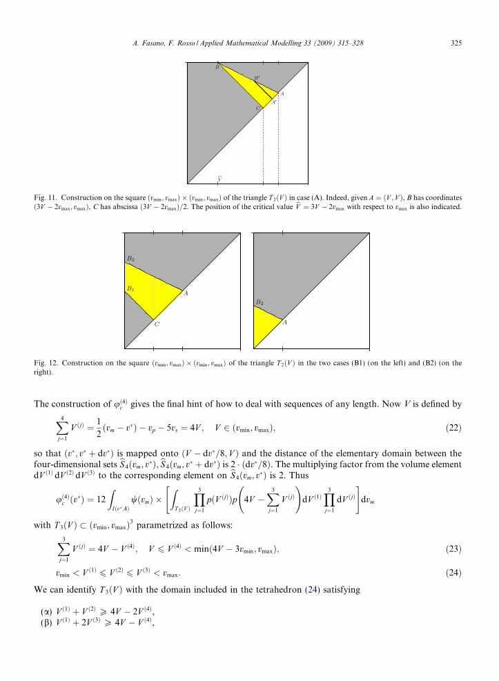
Fig. 11. Construction on the square ðvmin; vmaxÞ � ðvmin; vmaxÞ of the triangle T 2ðV Þ in case (A). Indeed, given A ¼ ðV ; V Þ, B has coordinatesð3V � 2vmax; vmaxÞ, C has abscissa ð3V � 2vmaxÞ=2. The position of the critical value eV ¼ 3V � 2vmax with respect to vmax is also indicated.

Fig. 12. Construction on the square ðvmin; vmaxÞ � ðvmin; vmaxÞ of the triangle T 2ðV Þ in the two cases (B1) (on the left) and (B2) (on theright).


The construction of uð4Þc gives the final hint of how to deal with sequences of any length. Now V is defined by
X4
j¼1

V ðjÞ ¼ 1

2ðvm � v�Þ � vp � 5vs ¼ 4V ; V 2 ðvmin; vmaxÞ; ð22Þ

so that ðv�; v� þ dv�Þ is mapped onto ðV � dv�=8; V Þ and the distance of the elementary domain between thefour-dimensional sets bS 4ðvm; v�Þ; bS4ðvm; v� þ dv�Þ is 2 � ðdv�=8Þ. The multiplying factor from the volume elementdV ð1Þ dV ð2Þ dV ð3Þ to the corresponding element on bS 4ðvm; v�Þ is 2. Thus

uð4Þc ðv�Þ ¼ 12

ZIðv�;4Þ

wðvmÞ �Z

T 3ðV Þ

Y3

j¼1

pðV ðjÞÞp 4V �X3

j¼1

V ðjÞ !

dV ð1ÞY3

j¼1

dV ðjÞ" #

dvm

with T 3ðV Þ � ðvmin; vmaxÞ3 parametrized as follows:
X3
j¼1

V ðjÞ ¼ 4V � V ð4Þ; V 6 V ð4Þ < minð4V � 3vmin; vmaxÞ; ð23Þ

vmin < V ð1Þ 6 V ð2Þ 6 V ð3Þ < vmax: ð24Þ

We can identify T 3ðV Þ with the domain included in the tetrahedron (24) satisfying

(a) V ð1Þ þ V ð2Þ P 4V � 2V ð4Þ,(b) V ð1Þ þ 2V ð3Þ P 4V � V ð4Þ,

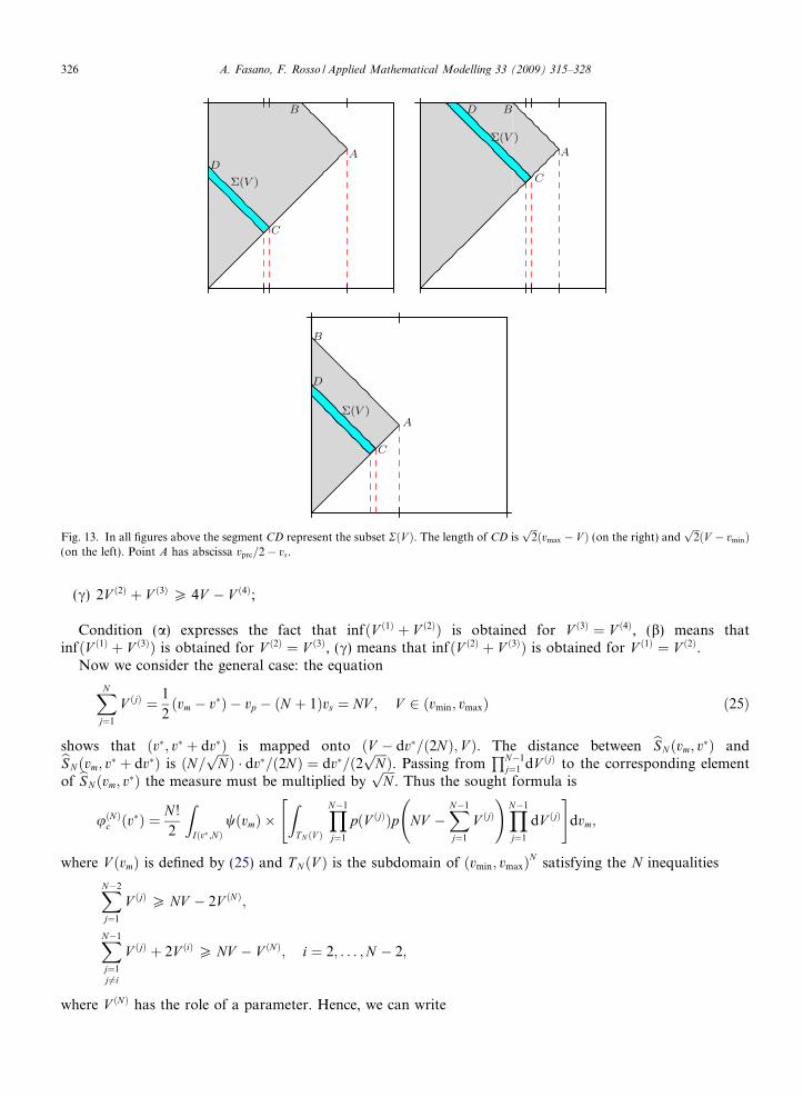
Fig. 13. In all figures above the segment CD represent the subset RðV Þ. The length of CD isffiffiffi2pðvmax � V Þ (on the right) and

ffiffiffi2pðV � vminÞ

(on the left). Point A has abscissa vprc=2� vs.


(c) 2V ð2Þ þ V ð3Þ P 4V � V ð4Þ;

Condition (a) expresses the fact that infðV ð1Þ þ V ð2ÞÞ is obtained for V ð3Þ ¼ V ð4Þ, (b) means thatinfðV ð1Þ þ V ð3ÞÞ is obtained for V ð2Þ ¼ V ð3Þ, (c) means that infðV ð2Þ þ V ð3ÞÞ is obtained for V ð1Þ ¼ V ð2Þ.

Now we consider the general case: the equation
XN
j¼1

V ðjÞ ¼ 1

2ðvm � v�Þ � vp � ðN þ 1Þvs ¼ NV ; V 2 ðvmin; vmaxÞ ð25Þ

shows that ðv�; v� þ dv�Þ is mapped onto ðV � dv�=ð2NÞ; V Þ. The distance between bSN ðvm; v�Þ andbSN ðvm; v� þ dv�Þ is ðN=ffiffiffiffiNpÞ � dv�=ð2NÞ ¼ dv�=ð2

ffiffiffiffiNpÞ. Passing from

QN�1j¼1 dV ðjÞ to the corresponding element

of bSNðvm; v�Þ the measure must be multiplied byffiffiffiffiNp

. Thus the sought formula is

uðNÞc ðv�Þ ¼N !

2

ZIðv�;NÞ

wðvmÞ �Z

T N ðV Þ

YN�1

j¼1

pðV ðjÞÞp NV �XN�1

j¼1

V ðjÞ !YN�1

j¼1

dV ðjÞ" #

dvm;

where V ðvmÞ is defined by (25) and T N ðV Þ is the subdomain of ðvmin; vmaxÞN satisfying the N inequalities
XN�2
j¼1

V ðjÞ P NV � 2V ðNÞ;

XN�1

j¼1j 6¼i

V ðjÞ þ 2V ðiÞ P NV � V ðNÞ; i ¼ 2; . . . ;N � 2;

where V ðNÞ has the role of a parameter. Hence, we can write


ucðv�Þ ¼XN ð0Þðv�Þ

N¼1

uðNÞc ðv�Þ: ð26Þ

In order to compute udðv�Þ we use the following argument. We consider the set of precursors of a residualdrop. These are the elongated bodies generated after a sequence of ordinary events and having volume inthe range ð2vmin þ vs; 2vmax þ 2vsÞ. We can calculate the distribution of precursors uprcðvprcÞ exactly as we havecalculated ucðv�Þ, i.e.

uprcðvprcÞ ¼XN ð0ÞðvprcÞ

N¼1

uðNÞc ðvprcÞ; vprc 2 ð2vmin þ 2vs; 2vmax þ 2vsÞ: ð27Þ

Next we analyze the terminating events leading from vprc to v� and corresponding to a cumulative volume

2V ¼ v1 þ v2 ¼ vprc � v� � 2vs ð28Þ

provided that

vprc � 2ðvmin þ vsÞ > v�: ð29Þ
For a given vprc, disregarding the size of the residual drop v�, the admissible pairs ðv1; v2Þ belong to the setTðvprcÞ, shown in Fig. 8. Eq. (28) defines a segment RðV Þ �TðvprcÞ.
Let us introduce the probability Fðv1; v2; vprcÞ defined over the domain TðvprcÞ, normalized so that
ZTðvprcÞ
Fðv1; v2; vprcÞdv1dv2 ¼1

2:

At this point we proceed as usual. The interval ðv�; v� þ dv�Þ generates an infinitesimal strip in TðvprcÞ whosethickness is dv�=

ffiffiffi2p

. Introducing the coordinate n along RðV Þ (see Fig. 13), we perform the integrals
Z ffiffi2pðvmax�V Þ
0

F V � nffiffiffi2p ; V þ nffiffiffi

2p ; vprc

� �dn; if V >

vmin þ vmax

2ðcase ðaÞÞ;Z ffiffi

2pðV�vminÞ

0

F V � nffiffiffi2p ; V þ nffiffiffi

2p ; vprc

� �dn; if V <

vmin þ vmax

2ðcase ðbÞÞ;

ð30Þ

which by means of the change of variable v1 ¼ V � n=ffiffiffi2p

become

2ffiffiffi2p Z V

ð2V�vmaxÞFðv1; V � v1; vprcÞdv1; if V >

vmin þ vmax

2ðcase ðaÞÞ;

2ffiffiffi2p Z V

vmin

Fðv1; V � v1; vprcÞdv1; if V <vmin þ vmax

2ðcase ðbÞÞ:

ð31Þ

Multiplying by ucðvprcÞð2dv�=ffiffiffi2pÞ we obtain the probability of the events leading from vprc to residual drops in

ðv�; v� þ dv�Þ, and the function udðv�Þ is finally got by integrating over the admissible range for vprc:

udðv�Þ ¼ 4

Z 2ðvmaxþvsÞ

2ðvminþvsÞþv�ucðvprcÞ

Z V

IðV ÞFðv1; V � v1; vprcÞdv1

" #dvprc;

where V is defined by (28) as a function of vprc, IðV Þ is exactly the same function given in (15), and (29) hasbeen taken into account in selecting the integration interval. Thus we have found

ures ¼ ua þ ub þ uc þ ud ð32Þ
and eventually
u ¼ uprm þ uord þ ures ð33Þ

is the distribution function of the droplets not belonging to the categories of maximal size primary drops andof satellite drops.


4. Averaging over sequences

We have already computed the probability P ðN ; vmÞ that a drop vm generates a sequence of N ordinaryevents. Thus we can calculate the average length of sequences originating from a parent vm

hNivm¼

XN2NðvmÞ

NP ðN ; vmÞ: ð34Þ

The average length of all sequences will be

hNi ¼Z V o

v1m

hNivmwðvmÞdvm: ð35Þ

We can also define the following quantities:

N c ¼Z vmax

vmin

ucðv�Þdv�; ð36Þ

N d ¼Z vmax

vmin

udðv�Þdv�; ð37Þ

counting the number of residual drops produced by a terminal or a constrained breakage, respectively. Ofcourse N c;Nd also count the number of sequences in the two classes. In this way we can determine the fractionof sequences terminating with a constrained breakage:

v ¼ N d

Nc þ Nd:

Acknowledgement

We wish to thank professor Stefano Guido of the Department of Chemical Engineering, Faculty of Engi-neering of the University of Napoli (Italy) for his comments and suggestions during the preparation of thispaper. We also wish to thank him for providing the movie of an experiment worked out in his departmentand from which Figs. 1–5 have been taken.

References

[1] A. Fasano, F. Rosso, Implementation of a fragmentation–coagulation-scattering model for the dynamics of stirred liquid–liquiddispersions, Physica D: Non Linear Phenom. 222 (1–2) (2006) 141–158 (special issue on Coagulation-fragmentation Processes).

[2] H. Stone, A. Stroock, A. Ajdari, Engineering flows in small devices microfluidics toward a lab-on-a-chip, Ann. Rev. Fluid Mech. 36(2004) 381–411.

[3] V. Cristini, S. Guido, A. Alfani, J. Blawzdziewicz, M. Loewenberg, Drop breakup and fragment distribution in shear flow, J. Rheol.47 (5) (2003) 1283–1298.

[4] Y. Renardy, V. Cristini, J. Li, Drop fragment distributions under shear with inertia, Int. J. Multiphase Flow 28 (7) (2002) 1125–1147.[5] V. Sibillo, G. Pasquariello, M. Simeone, V. Cristini, S. Guido, Drop deformation in microconfined shear flow, Phys. Rev. Lett. 97 (5)

(2006) 054502.[6] V. Cristini, J. Blawzdziewicz, M. Loewenberg, L.R. Collins, Breakup in stochastic stokes flows: sub-Kolmogorov drops in isotropic

turbulence, J. Fluid Mech. 492 (2003) 231–250.[7] V. Cristini, Y.C. Tan, Theory and numerical simulation of droplet dynamics in complex flows – a review, Lab on a Chip 4 (4) (2004)

257–264.[8] Y. Renardy, V. Cristini, Scalings for fragments produced from drop breakup in shear flow with inertia, Phys. Fluids 13 (8) (2001)

2161–2164.[9] Y.Y. Renardy, V. Cristini, Effect of inertia on drop breakup under shear, Phys. Fluids 13 (1) (2001) 7–13.

[10] V. Cristini, Y.Y. Renardy, Scaling for droplet sizes in shear-driven breakup: non-microfluidic ways to monodisperse emulsions, FluidDyn. Mater. Process. 2 (2) (2006) 77–94.

Modelling breakup process of a liquid drop in shear flow

Documents