Modelling Autoregressive Processes with a Shifting Mean

Modelling autoregressive processes with a shifting mean

Timo Terasvirta∗

Department of Economic StatisticsStockholm School of Economics

Andres Gonzalez

Banco de la Republica, ColombiaUnidad de investigaciones economicas

November 9, 2006

Abstract

This paper contains a nonlinear, nonstationary autoregressive model whose inter-cept changes deterministically over time. The intercept is a flexible function of time,and its construction bears some resemblance to neural network models. A modellingtechnique, modified from one for single hidden-layer neural network models, is devel-oped for specification and estimation of the model. Its performance is investigated bysimulation and further illustrated by two applications to macroeconomic time series.

Keywords: deterministic shift, nonlinear autoregression, nonstationarity, nonlineartrend, structural changeJEL Classification Codes: C22, C52

Acknowledgement:: This work has been supported by Jan Wallander’s and Tom Hedelius’s Foun-

dation, Grants No. J02-35 and P2005-0033:1. The paper has been presented at the workshop ”Nonlinear

Dynamical Methods and Time Series Analysis”, Udine, August/September 2006 and at the 14th SNDE

conference, Washington University, March 24-25, 2006. Material from the paper has also been discussed

in seminars at the European Central Bank, Frankfurt am Main, Bank of Finland, Helsinki, and Swedish

School of Economics and Business Administration, Helsinki. Comments from participants are gratefully

acknowledged. Our warmest thanks also to Birgit Strikholm for useful comments. The responsibility for

any errors and shortcomings in this work remains ours.

∗Department of Economic Statistics, Stockholm School of Economics, Box 6501, SE-113 83 Stockholm,Sweden, email: [email protected]

1 Introduction

There exist several methods of decomposing time series into components. Typically, one

of the components is called “trend”, and there may also be a cyclical component. When

a series is divided into these components, the “trend” is often extracted from the series

using a filtering procedure such as a two-sided moving average. The dynamic behaviour

of the trend-adjusted series is then modelled separately, and the results are conditional

on the filtered trend. For a recent overviews of filtering time series, see Canova (1998),

Baxter and King (1999), Morley (2000) and Morley, Nelson and Zivot (2003). Massmann,

Mitchel and Weale (2003) provide an overview of both smoothing, using a Kalman filter,

and filtering. It is also possible to assume that the series has a linear or perhaps quadratic

trend and estimate it jointly with the stochastic dynamic fluctuations in the series. The

fluctuations are then movements around this deterministic trend. In cases where this is

done, the series under study is most often a realization of a trending nonstationary process.

Sometimes a similar idea may be applied to series that do not “look” nonstationary in

the sense that they would seem to have a linear or quadratic trend. They may rather be

viewed as having a shift in the unconditional mean. In those cases a popular assumption

in econometrics has been that the underlying process has a break or breaks in the mean,

so the process is piecewise stationary. Some of the series may, however, be viewed as

having a smooth transition in the mean. These series may sometimes be relatively well

described by stationary autoregressive processes that contain a stationary root close to

the unit circle, although the data-generating process involves a deterministic shift in the

mean of the process.

Monthly European inflation series beginning around 1980 are a case in point. Their

early values are high but settle down in the 1990s, when the inflation rate keeps fluctuating

at a rather low level. This process may be characterized by an autoregressive model with

a near unit root and a starting-point far above the mean of the series. The role of this root

is to pull down the realization to the level where it fluctuates in the 1990s. Another view

would be to interpret the decrease in inflation as a downward shift in the unconditional

mean. This would imply that there have been changes in economic policy that are hard

to quantify and that have brought the inflation down. These changes are then proxied

by time and represented by a shifting mean in the autoregressive process. For more

discussion, see (Gonzalez, Hubrich and Terasvirta 2006). In the present paper we consider

an autoregressive model with a shifting mean that may be seen as a generalization of a

1

corresponding model with a single break or several breaks in the mean.

The autoregressive model with a shifting mean of the type we shall consider is similar

to a linear model with a polynomial trend in the sense that the parameters in the trend

are estimated jointly with other parameters. It differs from the smoothing and filtering

approaches, in which the series is first smoothed (components removed) or filtered, and

the remaining analysis is conditional on this step. The approach closest to ours is that

of Bierens (1997, 2000). Bierens (1997) derived a Dickey-Fuller test (Dickey and Fuller

(1979)) against the hypothesis of nonlinear trend stationarity in which the nonlinear trend

is approximated prior to testing by Chebyshev polynomials. Bierens (2000) developed

nonparametric tests of co-trending, a situation that occurs when a pair of series that are

stationary around a nonlinear trend follow each other closely, so that they share a common

trend. Our approach will also allow us to compare different series with shifting means and

see if the shifts are in some sense similar across series. This extension is, however, left for

further work.

The plan of the paper is as follows. The autoregressive model with a shifting mean

is presented in Section 2, and specification issues are dealt with in Section 3. Section 4

contains results of a Monte Carlo experiment, and empirical examples can be found in

Section 5. Section 6 concludes.

2 Nonlinear deterministic trend stationary models

The stationary autoregressive (AR) model with a shifting mean (SM) of order p [SM-

AR(p)] model, can be written as

yt = δ(t) +

p∑

j

θjyt−j + εt (1)

where the roots of the lag polynomial 1 −∑

θjLj lie outside the unit circle, {εt} is the

sequence of normal independent (0, σ2) errors and δ(t) is a deterministic nonlinear shift

function. It is often assumed that δ(t) is linear function of t in which case (1) is typically

called “trend-stationary”. Sometimes, however, the functional form of δ(t) is unknown.

In this paper we define δ(t) as follows:

δ(t) = δ0 +

q∑

i=1

δig(γi, ci, t/T ) (2)

where δi, i = 1, . . . , q, are parameters and g(γi, ci, t/T ), i = 1, . . . , q, are logistic transition

functions:

g(γi, ci, t/T ) =(

1 + exp(

− γi(t/T − ci)))

−1(3)

2

with γi > 0, i = 1, ..., q. The components in the shift function (2) are exchangeable, and

identification is achieved for example by assuming c1 < · · · < cq. In applications, it may

be sometimes assumed that 0 ≤ ci ≤ 1, i = 1, ..., q, but that restriction is not required by

the statistical theory.

The shifting mean of yt at time t equals

Etyt = (1 −

p∑

j=1

θjLj)−1δ(t).

One may also parameterize the SM-AR model as follows:

yt = δ(t) +

p∑

j=1

θj{yt−j − δ(t − j)} + εt

in which case Etyt = δ(t).

The specification of δ(t) in (2) with (3) bears resemblance to the so called “single

hidden-layer” artificial neural network model. It follows that theoretically, any function

h(t) satisfying rather mild regularity conditions can be approximated arbitrarily accurately

by δ(t) such that q ≤ q0 < ∞ in (2). This has been discussed in several papers including

Cybenko (1989) and Hornik, Stinchcombe and White (1989).

The parametric form of (2) is very flexible and contains as special cases well known

examples of nonlinear trends. For instance, when δ1 = · · · = δq = 0, (2) becomes constant,

and when q = 1, δ(t) changes smoothly from δ0 to δ0 + δ1 as a function of t, with the

centre of the change at t = c1T . The smoothness of the change is controlled by γ1: the

larger γ1 the faster the transition. When γ1 → ∞, δ(t) collapses into a step function, so

there is a single break in the intercept. On the contrary, when γ is small, δ(t) represents

a slow shift that around c is approximately linear. Values q > 1 add flexibility to δ(t).

For example, when q = 2, γ1 = γ2, c1 < c2 and δ1 = −δ2 in (2), δ(t) changes from δ0 at

the beginning of the sample to δ0 + δ1 for t ∈ (c1T, c2T ) and back towards δ0 for t > c2T .

This kind of symmetric change in the intercept can also be approximated with a logistic

function with a second-order exponent as explained in Terasvirta (1998) and Jansen and

Terasvirta (1996).

3 Model specification

In practical modelling situations, the form of the SM-AR model has to be determined from

the data. This implies selecting p and q. There is no natural order in which the choice is

made. It may be expected, however, that if p is selected first and there is a shifting mean,

3

appropriate selection criteria may sometimes choose a large p in order to accommodate the

shift. This may leave less room for a time-varying intercept. But then, if q is selected first,

it may in turn be large, as some of the stochastic variation may be ascribed to the shift

function. The order of selection may thus depend on the problem at hand. For example,

if there is economic theory suggesting that having a shifting mean may be an appropriate

solution, one may want to select q first. If this is not a case, choosing p first may be

the more appealing alternative of the two. The decision is left to the model builder.

Nevertheless, when q is selected first, one may use a heteroskedasticity-autocorrelation

consistent (HAC) estimator for the covariance matrix of the estimators throughout the

model selection process and thus account for the fact that the conditional mean may also

be time-varying.

3.1 QuickShift: a procedure for determining the number of transition

functions

Determining q in (2) may be done either by a sequence of specification tests or by model

selection criteria. We shall suggest a procedure that we call QuickShift. It is a simplified

form of a procedure that White (2006) recently proposed for specifying and estimating

artificial neural network models and that he called QuickNet. QuickShift as well as Quick-

Net have two useful properties. First, they transform the model selection problem into a

problem of selecting variables, which simplifies the computations. Second, overfitting is

avoided.

The origins of QuickNet lie in a result by Bierens (1990), saying that under very general

conditions E(εt|xt) 6= 0 implies that E(εt exp(x′

tθ)) 6= 0 for θ ∈ Θ. This means that when a

model is misspecified, the disturbance εt is correlated with functions of the form exp(x′

tθ)

for any θ ∈ Θ. Stinchcombe and White (1998) generalized this result and showed that it

holds for a very general family of functions, including the logistic function. It follows that

exp(x′

tθ) can be replaced by any function of the form G(x′

tθ) = (1 + exp {−x′

tθ})−1. In

fact, polynomial functions form perhaps the most important exception to this rule.

White (2006) uses the results of Stinchcombe and White (1998) to construct a sequen-

tial procedure for specifying a neural network model. The idea is simple: given a finite set

of hidden units that are logistic functions, the algorithm selects the subset of them that

gives the largest in-sample predictive power. The selection procedure is sequential: the

hidden unit with the largest correlation with the predictive error is selected at each step.

The algorithm stops when the predictive power of the marginal unit is sufficiently small.

4

QuickNet requires specifying a priori a maximum number of hidden units and a large

set of candidate functions. The maximum number of hidden units q can be set to any

value such that the model can be estimated, given the sample size. Applying White’s

idea to the present situation results in QuickShift. The hidden units are simply replaced

by logistic transition functions of type (3). The set of transition functions is obtained by

evaluating (3) over a fixed grid for γ and c. A feasible grid may be defined as follows:

ΘN = {(ΓNγ × CNc)} with ΓNγ = {γs : γs = κγs−1, s = 1, . . . ,Nγ , κ ∈ (0, 1)} and

CNc = {cs : cs = cs−1 + (1/Nc), s = 1, . . . ,Nc}.

Given q and ΘN , QuickShift consists of the following steps:

1. Estimate model (1) assuming δ(t) = δ0, save the residuals εt,0.

2. After selecting q − 1 transitions, q > 1, choose the transition function that has the

largest correlation with εt,q−1 that is, let

(γ, c)q = argmax(γs,cs)∈ΘN[r(g(γs, cs, t/T ), εq−1,t)]

2

where r(., .) is the sample correlation between g(γs, cs, t/T ) and

εq−1,t = yt − δ0 −

q−1∑

i=1

δig(γi, ci, t/T ) −

p∑

j=1

θjyt−j

3. Given (γ, c)q, obtain the estimates (δ0, . . . , δq, θ1, . . . , θq)′ by OLS. Save εq,t and

compute the value of the Bayesian Information Criterion (BIC), call it BIC(q).

4. Continue until q > q and choose q such that q = argminq∈(1,...,q)BIC(q).

The above description of QuickShift uses BIC as the criterion for determining q, but

other decision rules are possible. White (2006) uses a consistent cross-validation criterion

proposed by Racine (1997, 2000). In the present context this cross-validation criterion has

two problems. First, it increases the computational burden of the algorithm. Second, in

some situations computing the value of the cross-validation criterion is not possible. The

reason is that when the validation sample is large, the moment matrix for the estimation

sample can be near-singular. Near-singularity in the moment matrix is likely to occur

when two or more transition functions have similar location parameters and the slope

parameters are not sufficiently different from each other.

In another variant of QuickShift, tests for parameter nonconstancy are used as the

criterion for determining q. In this case, after adding a transition to the model a test

5

for remaining intercept nonconstancy is carried out and testing is continued sequentially

until the first non-rejection of the constancy hypothesis. We consider two tests available

for testing intercept nonconstancy. They are the Taylor expansion based test by Lin and

Terasvirta (1994) and the Neural Network test by Lee, White and Granger (1993).

The increasing sequence of dependent tests in applying QuickShift means that the

nominal size of the overall sequence is not known, although an upper bound for it can be

computed. In order to favour parsimony we suggest a decreasing sequence of significance

levels. That is, the algorithm is started with a relatively large significance level α0 = 0.5,

say, and is subsequently decreased following the rule αs+1 = ταs where s is the current

step of the algorithm, and τ ∈ (0, 1). When α0 is large, τ should be relatively small,

τ = 0.5, for example.

3.1.1 Taylor expansion based parameter constancy test

Assume for a moment that p has been specified and consider testing for a time-varying

intercept in (1). This testing situation is a nonstandard one, because under the null

hypothesis there are unidentified nuisance parameters in the model. Under the null hy-

pothesis H0 : γi = 0, i = 1, . . . , q, and so ci, i = 1, . . . , q, are unidentified. Furthermore,

while δ∗i = δ0+(1/2)∑q

i=1 δi can be estimated consistently, this is not true for the elements

of the sum. Lin and Terasvirta (1994) circumvent this identification problem by replacing

δ(t) in (2) with Taylor expansions of g(γi, ci, t/T ) around γi = 0, reparameterizing (1),

and testing H0 : δ(t) = δ0 as H10 : φi = 0, i = 1, . . . ,m, in the auxiliary regression

yt = δ∗0 +

m∑

i=1

φi(t/T )i + θ′wt + ε∗t (4)

where wt = (yt−1, . . . , yt−p)′, ε∗t = εt + R(t/T ), and R(t/T ) is the remainder of the Taylor

expansion. Note that the asymptotic theory is not affected by the Taylor expansion,

because under H10; ε∗t = εt. The null hypothesis H1

0 can be tested using the standard LM

statistic or its F-version. Under H10 the LM statistic has an asymptotic χ2 distribution

with m degrees of freedom, and the F-statistic is approximately distributed as F (m,T −

kp−m− 1). See Lin and Terasvirta (1994) and Granger and Terasvirta (1993) for details

on how to compute these statistics.

In order to carry out the test, one has to choose m. Lin and Terasvirta (1994) suggest

m = 3, but in the present context larger values of m may be considered depending on

how smooth the deterministic component has to be in order to be an adequate description

of the shifting mean. For example, it may be that m = 3 does not lead to a rejection

6

of the null hypothesis, whereas m = m0 > 3 will. A similar argument is used in Bierens

(1997) to determine the order of the Chebyshev polynomial of time used to approximate

the nonlinear trend. This procedure assumes that there is no serial correlation in the

errors. If the specification search is initiated by erroneously assuming p = 0, then the test

statistic should be computed using an HAC estimator for the error covariance matrix.

The parameter constancy test based on (4) can be used sequentially for determining the

number of transition functions in (2). This is possible because the test can be applied to

a model in which δ(t) has been already estimated, and the question then is whether this

specification adequately captures the intercept nonconstancy. Eitrheim and Terasvirta

(1996) generalized the test by Lin and Terasvirta (1994) to this situation. For ease of

presentation, assume that model (1) with q = 1 has been estimated and adding a new

transition function to it is considered. The extended model is

yt = δ0 + δ1g(γ1, c1, t/T ) + δ2g(γ2, c2, t/T ) + θ′wt + ε∗t (5)

where g(γ2, c2, t/T ) is defined in (3). The null hypothesis of no remaining intercept non-

constancy is H0 : γ2 = 0. The testing problem is again nonstandard because δ2 and c2

are not identified when H0 is true. The Taylor expansion approximation is applied again

and the null hypothesis H0 : γ2 = 0 becomes H10 : δ∗2i = 0, i = 1, . . . ,m, in the auxiliary

regression,

yt = δ∗0 + δ1g(γ1, c1, t/T ) +m

∑

i=1

δ∗2i(t/T )i + θ′wt + ε∗t . (6)

As before, the test can be computed using the standard LM test or its F-approximation.

Under the null hypothesis, the LM statistic is asymptotically χ2-distributed with m degrees

of freedom while the corresponding F statistic has an approximate F(m,T − kp − m)

distribution.

3.1.2 The neural network test

The neural network test is an LM test of H0 : δi = 0, i = 1, . . . , q in (2). This choice of

null hypothesis leaves γi, and ci, i = 1 . . . , q, unidentified when H0 holds. Lee et al. (1993)

solve the identification problem by drawing the unidentified parameters γi, ci, i = 1, . . . , q,

from a uniform distribution and testing H0 with an LM test for each draw where the LM

statistic has an asymptotic χ2 distribution with q degrees of freedom. As the neural

network tests involves several draws of γi and ci, i = 1, . . . , q, one ends up with a sequence

of dependent p-values. In this case, the Bonferroni inequality provides an upper bound

for the p-value of the composite statistic. Let p1, . . . , ps be the p-values corresponding to

7

s test statistics, and P(1), . . . , P(s) the ordered p-values. The Bonferroni inequality leads

to rejection of H0 at α level if P(1) ≤ α/s. Since it is based on the smallest p-value it may

cause a power loss in the test. In applications the number of draws is not usually large.

Lee et al. (1993) use s = 5 in their empirical application.

In this paper the Neural Network test is used for detecting remaining intercept non-

constancy after a number of transition functions have been added to (2). This implies

that in order to carry out the test one has to define a ceiling q for the number of transition

functions that can be included in the model. In this paper, q = 5.

4 Estimation

Once the number of transitions in (2) has been selected, the parameters of the model can

be estimated. However, full estimation of the model parameters can be a challenging task.

The reason is that in small samples the log-likelihood function of an SM-AR(p) model

typically has a complicated surface with nearly flat regions and a large number of local

maxima.

Fortunately, full estimation of parameters may not be necessary in the present context,

because QuickShift in general provides good approximations to maximum likelihood esti-

mates. However, when exact maximum likelihood estimates are considered necessary, po-

tential numerical problems may be solved by applying a global optimization algorithm such

as simulated annealing and using the vector of parameters (γ ′, c′)′ where γ = (γ1, . . . , γq)′

and c = (c1, . . . , cq)′, selected by QuickShift as starting-values. Brooks and Morgan (1995)

and Goffe, Ferrier and Rogers (1994) contain useful expositions of simulated annealing.

5 Monte Carlo Experiment

In this section we investigate the properties of QuickShift by simulation. In particular,

we concentrate ourselves on the effect that different criteria for selecting the number of

transitions will have on the performance of the algorithm. As mentioned in Section 3.1,

BIC, Cross-Validation criteria or a sequence of parameter constancy tests may be used in

connection with QuickShift. As a benchmark to our algorithms we present result based on

the sequential procedure by Bai and Perron (1998), designed for selecting the number of

breaks.

When parameter constancy tests are applied, setting up QuickShift requires deciding

upon the order on which p and q are selected. If one selects q first, an HAC estimator

8

for the co-variance matrix should be used when computing the value of the test statistic.

The second decision to be taken is whether or not use a rapidly decreasing sequence of

significance levels. If this is done, the selection may started with a rather large initial

nominal level. Alternatively, a low nominal level or a sequence of slowly decreasing levels

may be used throughout the selection procedure. Examples of both cases will be given.

Furthermore, we consider the situation in which p = 1 prior to selecting q and another

case in which q is selected assuming p = 1. In simulations where the significance level

is sequentially decreased, the algorithm is started with α0 = 0.5 and is decreased by a

factor τ = 0.5 after each rejection. In the constant size simulations α0 = 0.05. Finally,

since the test by Lin and Terasvirta can be computed using different values of m in (4),

we simulate the procedure with both m = 3 and m = 6 in order to investigate the effect

that the polynomial approximation has on QuickShift.

The data-generating processes are defined as follows:

yt = 0.1+0.7g(t/T, γ1 = 3, c1 = 0.33)−0.7g(t/T, γ2 = 2, c2 = 0.67)+ρyt−1+ǫt (Model 1)

yt = 0.1+0.3g(t/T, γ1 = 3, c1 = 0.25)+0.5g(t/T, γ2 = 3, c2 = 0.75)+ρyt−1+ǫt (Model 2)

yt =0.1 + ǫt for 0 < t/T ≤ 0.5, (Model 3)

=0.3 + ǫt for 0.5 < t/T ≤ 1,

yt =δ0 + δ1(t/T ) + ǫt for 0 < t/T ≤ 0.2, (Model 4)

=δ0 + 0.2δ1 + ǫt for 0.2 < t/T ≤ 1,

where δ0 = 0.5, δ1 = −0.2δ0, ρ is either 0 or 0.5, g(.) is defined in (3) and ǫt ∼ N(0, 0.2).

In Models 1 and 2, the shift in the mean is smooth, whereas it is abrupt in Model 3. Model

4 is a mixture of these two types in the sense that the shift is smooth, except that there

is a point of discontinuity at t/T = 0.2. The sample sizes are T = 150 and T = 300. The

results are based on 1000 replications from each model.

Figure 1 presents the shifting means for the four models when ρ = 0. The mean shift

in Model 1 starts and ends at the same value and the mean is largest in the middle of the

sample. This type of shift should be easily estimated by QuickShift as it satisfies (2) when

q = 2. The shift in Model 2 is somewhat more difficult to approximate because it may

already be well approximated by a single transition function instead of two, the number

of transitions in the data-generating mechanism. As already mentioned, Model 3 has a

9

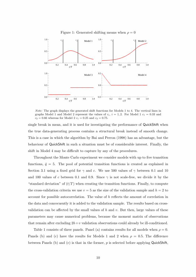
Figure 1: Generated shifting means when ρ = 0

0.2 0.4 0.6 0.8 1.00.0

0.5

1.0 c1 c2 Model 1

t/T0.2 0.4 0.6 0.8 1.0

0.0

0.5

1.0 c1 c2 Model 2

t/T

0.2 0.4 0.6 0.8 1.00.0

0.5

1.0Model 3

t/T0.2 0.4 0.6 0.8 1.0

−0.5

0.0

0.5Model 4

t/T

Note: The graph displays the generated shift functions for Models 1 to 4. The vertical lines ingraphs Model 1 and Model 2 represent the values of ci, i = 1, 2. For Model 1 c1 = 0.33 andc2 = 0.66 whereas for Model 2 c1 = 0.25 and c2 = 0.75.

single break in mean, and it is used for investigating the performance of QuickShift when

the true data-generating process contains a structural break instead of smooth change.

This is a case in which the algorithm by Bai and Perron (1998) has an advantage, but the

behaviour of QuickShift in such a situation must be of considerable interest. Finally, the

shift in Model 4 may be difficult to capture by any of the procedures.

Throughout the Monte Carlo experiment we consider models with up to five transition

functions, q = 5. The pool of potential transition functions is created as explained in

Section 3.1 using a fixed grid for γ and c. We use 500 values of γ between 0.1 and 10

and 100 values of c between 0.1 and 0.9. Since γ is not scale-free, we divide it by the

“standard deviation” of (t/T ) when creating the transition functions. Finally, to compute

the cross-validation criteria we use v = 5 as the size of the validation sample and h = 2 to

account for possible autocorrelation. The value of h reflects the amount of correlation in

the data and concecuently it is added to the validation sample. The results based on cross-

validation can be affected by the small values of h and v. But then, large values of these

parameters may cause numerical problems, because the moment matrix of observations

that remain after excluding 2h+v validation observations could already be ill-conditioned.

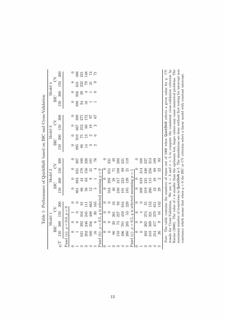
Table 1 consists of three panels. Panel (a) contains results for all models when ρ = 0.

Panels (b) and (c) have the results for Models 1 and 2 when ρ = 0.5. The difference

between Panels (b) and (c) is that in the former, p is selected before applying QuickShift,

10

whereas in the latter, q is selected first. It is seen from Panel (a) that when ρ = 0 and

T = 150 in Model 1, both BIC and CV find q = 2 more often than the other alternatives.

However, when T = 300, both criteria find more transitions, and for CV this tendency

is quite pronounced. For the other models, the outcome is somewhat different in that

the most frequent number of transitions is one and for BIC it does not increase with the

sample size. Even here, CV leads to less parsimonious models than BIC. For Model 2 the

correct number of transitions is two, but although CV often chooses q > 1, the dispersion

around q = 2 is large.

Selecting q under the assumption p = 0 makes a large difference compared to assuming

p = 1 when BIC is concerned, but CV yields rather similar results in both cases, at least

for Model 1. BIC is again more parsimonious than CV.

Results for QuickShift based on parameter constancy tests appear in Tables 2-4. The

tables contain two panels. In Panel (a), the significance level α0 = 0.5 for all tests. In

Panel (b), α0 = 0.05 and τ = 0.5, so the significance level is halved at each step. Three

test statistics are considered. LTj is the Lin and Terasvirta (LT) statistic with m = j,

j = 3, 6, and NN is the Lee, White and Granger neural network test with the Bonferroni

bound. In Table 2, it is assumed that ρ = 0. Table 3 contains results for the case ρ = 0.5

when the lag length in the autoregressive null model equals one. In Table 4, ρ = 0.5

and the test statistics are calculated using Andrews’s HAC estimator for the covariance

matrix.

The results in these tables indicate that parameter constancy tests perform better

than either BIC or CV. In this experiment, the constant significance level leads to more

parsimonious models than a sequence of decreasing levels. This result does not generalize,

however, as it is dependent on the initial significance level α0 which is quite high, α0 = 0.5.

Lowering it increases parsimony. From Table 2 it is seen that generally there is no big

difference between the LT and NN tests. There is one exception, however. When there

is a single break in the mean (Model 3), NN finds q = 1 more often than the two LT

tests. This is due to the difficulty of approximating a break with a polynomial of time.

LT3 is generally more parsimonious than LT6, but in some situations (Model 4 with a

discontinuity in the mean, Panel (b)) a sixth-order polynomial seems superior to a third-

order one. Comparing Tables 3 and 4 it seems that applying the HAC covariance matrix

sharpens the results. The choice is more focused on a single value of q than it is if the

presence of yt−1 in the model is ignored.

Table 5 contains results from the sequential selection procedure of Bai and Perron

11

(1998) (BP). This table is also divided into two panels. In Panel (a), the results concern

all models, assuming ρ = 0 in Models 1 and 2. Data for results in Panel (b) have been

generated only from Models 1 and 2 with ρ = 0.5. The alternative before selecting q are

p = 0 with the HAC estimator and p = 1 without it. Two significance levels, α = 0.05 and

α = 0.1 are used in this experiment. The results are sensitive to the choice between p = 0

(with HAC) or p = 1 (without HAC), the latter leading to a greater number of breaks

than the former. An interesting fact is that a single break (Model 4) is equally easily

found by, say, the NN test and QuickShift, as it is with the BP procedure. For Model 1,

BP selects either q = 0 or q = 2 when T = 150 but favours q ≥ 2 when T = 300. This

type of shift is obviously not easy to approximate by breaks.

So far we have reported results concerning the number of transitions found using Quick-

Shift as well breaks detected by BP. There are, however, qualitative differences between

the former and the latter. Figure 2 displays estimated shifting intercepts based on a sin-

gle time series generated from each of the four models. We also present the estimated

shift obtained using tenth-order Chebyshev polynomials because these polynomials are

commonly applied to approximating nonlinear functions. As is seen from the figure, the

approximating properties of our flexible intercept (2) are generally quite good compared

to the Chebyshev polynomial and BP. In particular, our model is vastly superior to the

polynomial approximation at both ends of the sample. Naturally, BP is superior to the

other methods when it comes to Model 3 that contains a break in the mean. It offers a

rather crude approximation when the shifting mean is smooth as in Models 1 and 2 and

is not very good on the downward sloping stretch of Model 4. A general conclusion is

that our SM-AR model is a useful tool when it comes to parameterizing autoregressive

processes with a shifting mean.

6 Applications

6.1 The series

In this section we present two applications of QuickShift in order to illustrate its proper-

ties. The first application is related to Garcia and Perron (1996), Bai and Perron (2003)

and Zeileis and Kleiber (2005). It consists of estimating the shifting mean of a US ex-post

real interest rate series. More precisely, the time series is the US ex-post real interest

rate, defined as the three-month Treasury bill rate deflated by the consumer price in-

dex (CPI) inflation rate. The series contains 103 quarterly observations for the period

12

Tab

le1:

Per

form

ance

ofQ

uic

kShift

bas

edon

BIC

and

Cro

ss-V

alid

atio

n

Model

1M

odel

2M

odel

3M

odel

4B

ICC

VB

ICC

VB

ICC

VB

ICC

Vq/

T150

300

150

300

150

300

150

300

150

300

150

300

150

300

150

300

Panel

(a):

ρ=

0.0

,p

=0

00

01

00

00

00

00

00

08

01

10

00

861

883

631

307

895

910

667

389

888

956

641

486

2621

392

316

61

66

44

178

100

86

75

252

275

94

39

232

221

3202

246

245

111

56

63

156

326

14

13

60

172

16

479

148

4160

356

408

663

12

931

191

32

19

97

11

31

74

516

630

165

51

476

20

267

10

971

Panel

(b):

ρ=

0.5

,q

isse

lect

edass

um

ing

p=

0

00

00

00

00

01

00

00

344

293

651

331

286

20

261

43

40

28

71

49

3158

74

227

93

240

317

188

280

4496

701

459

644

191

223

69

221

5260

205

53

220

185

139

21

119

Panel

(c):

ρ=

0.5

,q

isse

lect

edass

um

ing

p=

1

00

06

00

00

01

00

40

409

619

314

168

2402

265

274

55

319

245

340

237

3318

309

321

152

200

115

256

313

4254

417

379

651

43

19

68

189

526

916

142

29

222

93

Note

:T

he

table

conta

ins

the

num

ber

sof

tim

esout

of

1000

when

Quic

kShift

sele

cts

agiv

enva

lue

for

q.

CV

stands

for

Cro

ss-V

alidation.

We

use

h=

3and

v=

5to

com

pute

the

consist

ent

cross

-validation

criter

ion

by

Raci

ne

(2000).

The

valu

eofv

issm

aller

than

the

optim

um

but,

larg

erva

lues

may

cause

num

eric

alpro

ble

ms.

The

maxim

um

num

ber

oftr

ansitions

inQ

uic

kShiftis

5.

The

sim

ula

tions

are

done

without

firs

tte

stin

gfo

rin

terc

ept

non

const

ancy

whic

hm

eans

that

when

q=

0th

eB

ICor

CV

criter

ion

sele

cta

linea

rm

odel

with

const

ant

inte

rcep

t.

13

Table 2: Performance of QuickShift based on different parameter con-stancy tests assuming ρ = 0

Model 1 Model 2 Model 3 Model 4q LT3 LT6 NN LT3 LT6 NN LT3 LT6 NN LT3 LT6 NN

Panel (a): α0 = 0.05, τ = 1

T = 1500 0 1 0 0 0 0 0 1 1 0 3 41 2 7 15 962 920 958 939 943 971 965 967 9802 913 864 902 27 50 29 50 34 23 34 25 153 64 97 71 9 24 12 9 12 3 1 3 14 19 26 12 2 5 1 2 9 0 0 1 05 2 5 0 0 1 0 0 1 2 0 1 0

T = 3000 1 5 0 0 1 0 0 2 2 0 0 01 0 0 0 942 883 927 898 923 938 981 983 9922 882 503 656 40 58 50 79 51 43 18 9 63 67 365 272 17 48 20 22 15 13 1 8 24 49 115 70 1 9 3 1 6 3 0 0 05 1 12 2 0 1 0 0 3 1 0 0 0

Panel (b): α0 = 0.5, τ = 0.5

T = 1500 0 0 0 0 0 0 0 1 1 0 0 01 0 1 1 823 691 835 738 722 872 798 841 9262 835 688 830 131 196 119 215 211 100 183 129 653 132 257 157 43 99 43 40 49 17 18 25 94 31 49 12 2 13 3 6 15 6 1 5 05 2 5 0 1 1 0 1 2 4 0 0 0

T = 3000 0 0 0 0 0 0 1 1 1 0 0 01 0 0 0 782 592 765 621 668 790 845 875 9302 795 287 468 151 242 164 293 255 158 139 104 553 123 528 438 64 147 66 78 57 41 14 19 144 81 175 93 3 16 5 7 15 9 4 2 15 1 10 1 0 3 0 0 4 1 0 0 0

Note: The columns LT3 and LT6 contain results for Taylor expansion based testwhen m = 3 or m = 6 in (4), whereas results for the Neural Network test arereported in column NN. α0 is the initial nominal level in the sequential procedure,τ is the adjustment factor. The nominal level is adjusted following αs = ταs−1,s = 1, . . . , 5. Data for models 1 and 2 was generated assuming ρ = 0.0 and alltests are computed without including lags of yt into the null model.

14

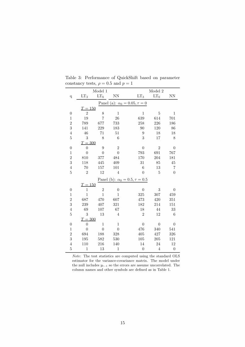
Table 3: Performance of QuickShift based on parameterconstancy tests, ρ = 0.5 and p = 1

Model 1 Model 2q LT3 LT6 NN LT3 LT6 NN

Panel (a): α0 = 0.05, τ = 0

T = 1500 2 8 1 1 5 11 19 7 26 639 614 7012 789 677 733 258 226 1863 141 229 183 90 120 864 46 71 51 9 18 185 3 8 6 3 17 8

T = 3000 0 9 2 0 2 01 0 0 0 793 691 7672 810 377 484 170 204 1813 118 445 409 31 85 454 70 157 101 6 13 75 2 12 4 0 5 0

Panel (b): α0 = 0.5, τ = 0.5

T = 1500 1 2 0 0 3 01 1 1 1 325 307 4592 687 470 607 473 420 3513 239 407 321 182 214 1514 69 107 67 18 44 335 3 13 4 2 12 6

T = 3000 0 1 1 0 0 01 0 0 0 476 340 5412 694 188 328 405 427 3263 195 582 530 105 205 1214 110 216 140 14 24 125 1 13 1 0 4 0

Note: The test statistics are computed using the standard OLSestimator for the variance-covariance matrix. The model underthe null includes yt−1 so the errors are assume uncorrelated. Thecolumn names and other symbols are defined as in Table 1.

15

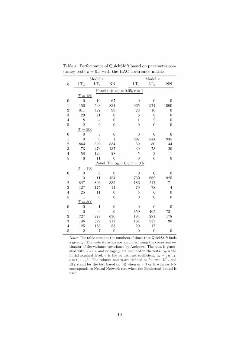
Table 4: Performance of QuickShift based on parameter con-stancy tests ρ = 0.5 with the HAC covariance matrix

Model 1 Model 2q LT3 LT6 NN LT3 LT6 NN

Panel (a): α0 = 0.05, τ = 1

T = 1500 0 10 67 0 0 01 150 538 834 965 974 10002 811 427 99 28 16 03 29 21 0 6 8 04 8 4 0 1 2 05 2 0 0 0 0 0

T = 3000 0 3 0 0 0 01 0 0 1 897 844 9352 863 590 834 59 80 443 73 273 137 39 73 204 58 123 28 5 3 15 6 11 0 0 0 0

Panel (b): α0 = 0.5, τ = 0.5

T = 1500 0 0 0 0 0 01 0 11 154 730 669 9252 847 803 835 186 247 713 127 175 11 79 78 44 25 11 0 5 6 05 1 0 0 0 0 0

T = 3000 0 1 0 0 0 01 0 0 0 659 465 7312 727 278 630 184 281 1783 146 529 317 137 237 904 125 185 53 20 17 15 2 7 0 0 0 0

Note: The table contains the numbers of times that QuickShift findsa given q. The tests statistics are computed using the consistent es-timator of the variance-covariance by Andrews. The data is gener-ated with ρ = 0.5 and no lags yt are included in the tests. α0 is theinitial nominal level, τ is the adjustment coefficient, αi = ταi−1,i = 0, . . . , 5. The column names are defined as follows: LT3 andLT6 stand for the test based on (4) when m = 3 or 6, whereas NNcorresponds to Neural Network test when the Bonferroni bound isused.

16

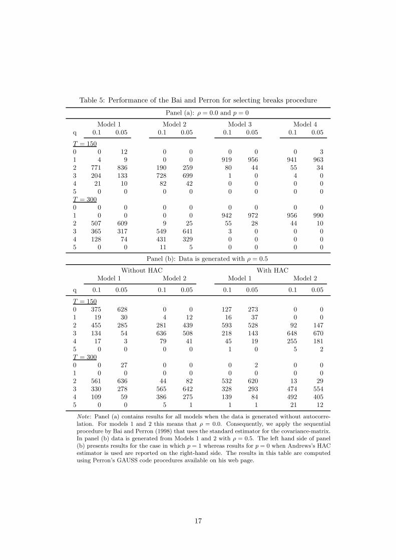
Table 5: Performance of the Bai and Perron for selecting breaks procedure

Panel (a): ρ = 0.0 and p = 0

Model 1 Model 2 Model 3 Model 4q 0.1 0.05 0.1 0.05 0.1 0.05 0.1 0.05

T = 1500 0 12 0 0 0 0 0 31 4 9 0 0 919 956 941 9632 771 836 190 259 80 44 55 343 204 133 728 699 1 0 4 04 21 10 82 42 0 0 0 05 0 0 0 0 0 0 0 0T = 3000 0 0 0 0 0 0 0 01 0 0 0 0 942 972 956 9902 507 609 9 25 55 28 44 103 365 317 549 641 3 0 0 04 128 74 431 329 0 0 0 05 0 0 11 5 0 0 0 0

Panel (b): Data is generated with ρ = 0.5

Without HAC With HACModel 1 Model 2 Model 1 Model 2

q 0.1 0.05 0.1 0.05 0.1 0.05 0.1 0.05

T = 1500 375 628 0 0 127 273 0 01 19 30 4 12 16 37 0 02 455 285 281 439 593 528 92 1473 134 54 636 508 218 143 648 6704 17 3 79 41 45 19 255 1815 0 0 0 0 1 0 5 2T = 3000 0 27 0 0 0 2 0 01 0 0 0 0 0 0 0 02 561 636 44 82 532 620 13 293 330 278 565 642 328 293 474 5544 109 59 386 275 139 84 492 4055 0 0 5 1 1 1 21 12

Note: Panel (a) contains results for all models when the data is generated without autocorre-lation. For models 1 and 2 this means that ρ = 0.0. Consequently, we apply the sequentialprocedure by Bai and Perron (1998) that uses the standard estimator for the covariance-matrix.In panel (b) data is generated from Models 1 and 2 with ρ = 0.5. The left hand side of panel(b) presents results for the case in which p = 1 whereas results for p = 0 when Andrews’s HACestimator is used are reported on the right-hand side. The results in this table are computedusing Perron’s GAUSS code procedures available on his web page.

17

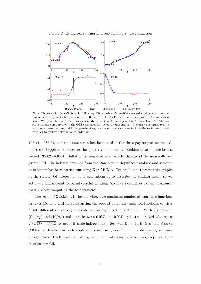
Figure 2: Estimated shifting intercepts from a single realization

0 100 200 300

0.00

0.25

0.50 Model 1

t

Bai and Perron True QuickShift Chebychev Pol

0 100 200 300

0.5

1.0 Model 2

t

0 100 200 300

0.0

0.2

0.4 Model 3

t0 100 200 300

0.00

0.25

0.50

Model 4

t

Note: The setup for QuickShift is the following: The number of transitions q is selected using sequentialtesting with LT3 as the test, where α0 = 0.05 and τ = 1. For Bai and Perron we used a 5% significancelevel. We generate one draw from each model with T = 300 and ρ = 0 in Models 1 and 2. All teststatistics are computed with the OLS estimator for the covariance matrix. In order to compare resultswith an alternative method for approximating nonlinear trends we also include the estimated trendwith a Chebychev polynomial of order 10.

1961(1)-1986(3), and the same series has been used in the three papers just mentioned.

The second application concerns the quarterly annualized Colombian inflation rate for the

period 1960(2)-2005(4). Inflation is computed as quarterly changes of the seasonally ad-

justed CPI. The index is obtained from the Banco de la Republica database and seasonal

adjustment has been carried out using X12-ARIMA. Figures 3 and 4 present the graphs

of the series. Of interest in both applications is to describe the shifting mean, so we

set p = 0 and account for serial correlation using Andrews’s estimator for the covariance

matrix when computing the test statistics.

The setup of QuickShift is the following. The maximum number of transition functions

in (2) is 15. The grid for constructing the pool of potential transition functions consists

of 500 different values of γ and c defined as explained in Section 3.1. With γ’s between

(0.1/σT ) and (10/σT ) and c are between 0.05T and 0.95T . γ is standardized with σT =

T/√

(T 2 − 1)/12 to make it scale-independent. See van Dijk, Terasvirta and Franses

(2002) for details. In both applications we use QuickShift with a decreasing sequence

of significance levels starting with α0 = 0.5 and adjusting αs after every rejection by a

fraction τ = 0.5.

18

6.2 Shifting mean of the US ex-post real interest rate

The number of transitions selected for the US interest rate series is reported in Table 6.3.

It has been selected assuming p = 0 and by carrying out the LT and NN test sequences

using Andrews’s estimator for the covariance matrix. As can be seen, QuickShift with BIC

selects a large number of transitions, six in all, whereas CV and the LT tests select two

and NN tests only find one. The fact that BIC selects a large number of transition may

be expected given the simulation results in Section 5. When we consider breaks, the Bai

and Perron procedure chooses three of them. This number of breaks in the US interest

rate series was also found by Bai and Perron (2003) and Zeileis and Kleiber (2005). It

differs from the outcome in Garcia and Perron (1996) who located two breaks.

Table 7 presents the selected transitions together with the estimated break dates. The

columns labelled ”Start”, ”Centre” and ”End” indicate the dates at which values of the qth

transition function begins to differ appreciably from zero, where the function takes value

0.5 and where it reaches one, respectively. For instance, the transition function of the first

transition begins to obtain values different from zero at 1968(1), the transition is centred

at 1972(2) and the function is practically equal to one after 1975(4). In other words, a

complete shift in the mean or regime change takes approximately seven years. The second

shift takes place in the second half of the sample. It has its centre at 1980(4) and spans over

a period of nine years. It is interesting to note that the centres of the transitions lie close to

the estimated break dates obtained by the Bai and Perron technique. Figure 3 shows the

estimated nonlinear means together with the selected transition functions (dashed lines).

The main difference between Bai and Perron’s mean and the one estimated with QuickShift

lies in the rate of adjustment towards a new level rather than in the levels themselves.

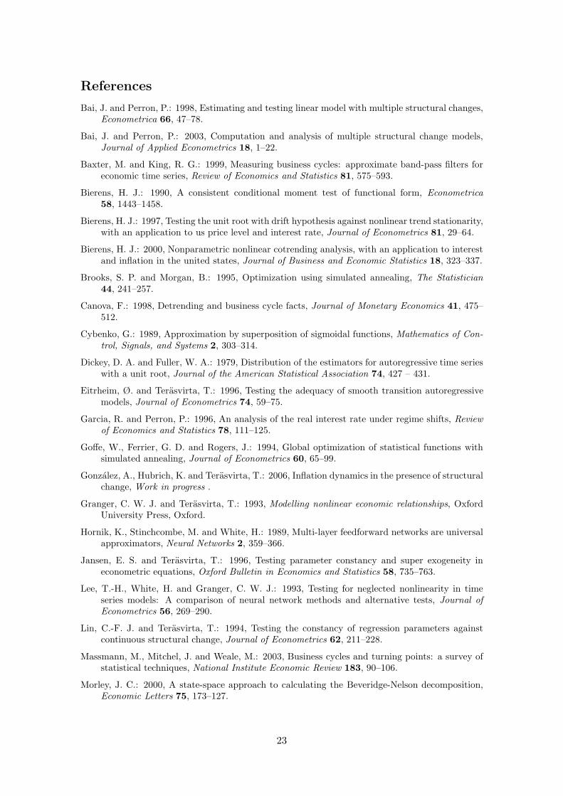
6.3 Shifting mean of the Colombian quarterly inflation rate

Results for the Colombian quarterly inflation are summarized in Tables 6.3 and 7 and

Figure 4. In this case, two transition functions are needed to capture the shifting mean.

The first one is centred at 1973(1) and the other at 1999(2). In the 1970s inflation increased

from around 10% to about 20% in more or less seven years, whereas the deceleration

process in the 1990s covers between 12 to 13 years and is about to be completed at the

end of the sample. A problem of interpretation arises when a transition is not completed by

the end of the observation period: will it continue or has a new level already been reached?

This is a forecasting problem not present when the shifting mean is characterized by breaks

in the intercept. But then, both approaches have a different problem: when will a new

19

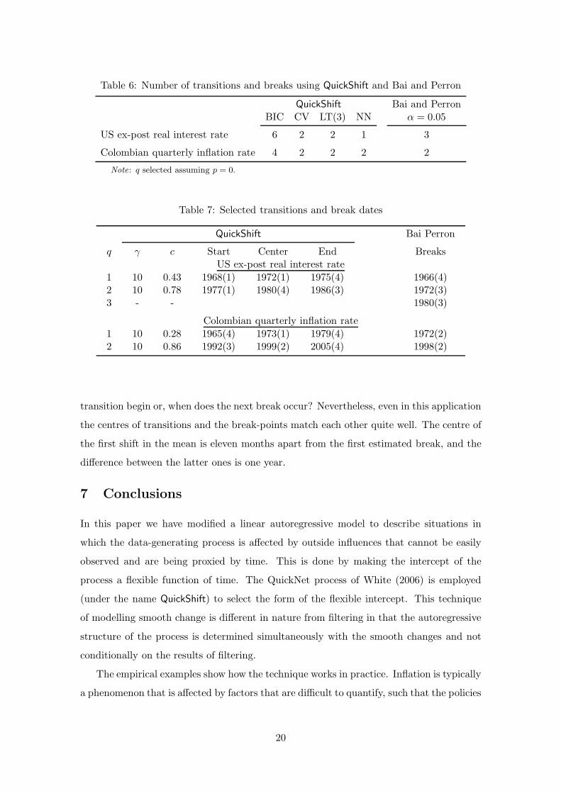
Table 6: Number of transitions and breaks using QuickShift and Bai and Perron

QuickShift Bai and PerronBIC CV LT(3) NN α = 0.05

US ex-post real interest rate 6 2 2 1 3

Colombian quarterly inflation rate 4 2 2 2 2

Note: q selected assuming p = 0.

Table 7: Selected transitions and break dates

QuickShift Bai Perron

q γ c Start Center End BreaksUS ex-post real interest rate

1 10 0.43 1968(1) 1972(1) 1975(4) 1966(4)2 10 0.78 1977(1) 1980(4) 1986(3) 1972(3)3 - - 1980(3)

Colombian quarterly inflation rate

1 10 0.28 1965(4) 1973(1) 1979(4) 1972(2)2 10 0.86 1992(3) 1999(2) 2005(4) 1998(2)

transition begin or, when does the next break occur? Nevertheless, even in this application

the centres of transitions and the break-points match each other quite well. The centre of

the first shift in the mean is eleven months apart from the first estimated break, and the

difference between the latter ones is one year.

7 Conclusions

In this paper we have modified a linear autoregressive model to describe situations in

which the data-generating process is affected by outside influences that cannot be easily

observed and are being proxied by time. This is done by making the intercept of the

process a flexible function of time. The QuickNet process of White (2006) is employed

(under the name QuickShift) to select the form of the flexible intercept. This technique

of modelling smooth change is different in nature from filtering in that the autoregressive

structure of the process is determined simultaneously with the smooth changes and not

conditionally on the results of filtering.

The empirical examples show how the technique works in practice. Inflation is typically

a phenomenon that is affected by factors that are difficult to quantify, such that the policies

20

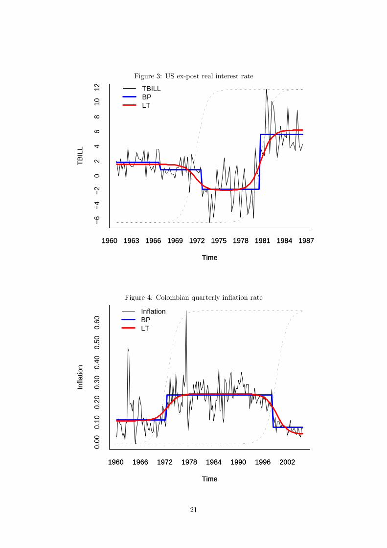
Figure 3: US ex-post real interest rate

Time

TB

ILL

1960 1963 1966 1969 1972 1975 1978 1981 1984 1987

−6

−4

−2

02

46

810

12 TBILLBPLT

Time

1960 1963 1966 1969 1972 1975 1978 1981 1984 1987

Figure 4: Colombian quarterly inflation rate

Time

Infla

tion

1960 1966 1972 1978 1984 1990 1996 2002

0.00

0.10

0.20

0.30

0.40

0.50

0.60

InflationBPLT

Time

1960 1966 1972 1978 1984 1990 1996 2002

21

of the central bank or institutional changes. The same is true for interest rates. The idea

that macroeconomic time series such as inflation and interest rates contain breaks has

been quite popular in econometric modelling, where the assumption of breaks has been

used to account for external influences such as changes in institutions. However, although

institutional changes in some situations can be abrupt, their effects on the series under

consideration may be distributed over a number of periods. The present applications show

how it is possible to obtain a more nuanced picture of deterministic changes in the series

by assuming that these changes can be smooth instead of just occurring abruptly at a

given moment of time.

22

References

Bai, J. and Perron, P.: 1998, Estimating and testing linear model with multiple structural changes,Econometrica 66, 47–78.

Bai, J. and Perron, P.: 2003, Computation and analysis of multiple structural change models,Journal of Applied Econometrics 18, 1–22.

Baxter, M. and King, R. G.: 1999, Measuring business cycles: approximate band-pass filters foreconomic time series, Review of Economics and Statistics 81, 575–593.

Bierens, H. J.: 1990, A consistent conditional moment test of functional form, Econometrica

58, 1443–1458.

Bierens, H. J.: 1997, Testing the unit root with drift hypothesis against nonlinear trend stationarity,with an application to us price level and interest rate, Journal of Econometrics 81, 29–64.

Bierens, H. J.: 2000, Nonparametric nonlinear cotrending analysis, with an application to interestand inflation in the united states, Journal of Business and Economic Statistics 18, 323–337.

Brooks, S. P. and Morgan, B.: 1995, Optimization using simulated annealing, The Statistician

44, 241–257.

Canova, F.: 1998, Detrending and business cycle facts, Journal of Monetary Economics 41, 475–512.

Cybenko, G.: 1989, Approximation by superposition of sigmoidal functions, Mathematics of Con-

trol, Signals, and Systems 2, 303–314.

Dickey, D. A. and Fuller, W. A.: 1979, Distribution of the estimators for autoregressive time serieswith a unit root, Journal of the American Statistical Association 74, 427 – 431.

Eitrheim, Ø. and Terasvirta, T.: 1996, Testing the adequacy of smooth transition autoregressivemodels, Journal of Econometrics 74, 59–75.

Garcia, R. and Perron, P.: 1996, An analysis of the real interest rate under regime shifts, Review

of Economics and Statistics 78, 111–125.

Goffe, W., Ferrier, G. D. and Rogers, J.: 1994, Global optimization of statistical functions withsimulated annealing, Journal of Econometrics 60, 65–99.

Gonzalez, A., Hubrich, K. and Terasvirta, T.: 2006, Inflation dynamics in the presence of structuralchange, Work in progress .

Granger, C. W. J. and Terasvirta, T.: 1993, Modelling nonlinear economic relationships, OxfordUniversity Press, Oxford.

Hornik, K., Stinchcombe, M. and White, H.: 1989, Multi-layer feedforward networks are universalapproximators, Neural Networks 2, 359–366.

Jansen, E. S. and Terasvirta, T.: 1996, Testing parameter constancy and super exogeneity ineconometric equations, Oxford Bulletin in Economics and Statistics 58, 735–763.

Lee, T.-H., White, H. and Granger, C. W. J.: 1993, Testing for neglected nonlinearity in timeseries models: A comparison of neural network methods and alternative tests, Journal of

Econometrics 56, 269–290.

Lin, C.-F. J. and Terasvirta, T.: 1994, Testing the constancy of regression parameters againstcontinuous structural change, Journal of Econometrics 62, 211–228.

Massmann, M., Mitchel, J. and Weale, M.: 2003, Business cycles and turning points: a survey ofstatistical techniques, National Institute Economic Review 183, 90–106.

Morley, J. C.: 2000, A state-space approach to calculating the Beveridge-Nelson decomposition,Economic Letters 75, 173–127.

23

Morley, J. C., Nelson, C. R. and Zivot, E.: 2003, Why are Beveridge-Nelson and unobserved-components decompositions of the GDP so different?, Review of Economics and Statistics

85, 235–243.

Racine, J.: 1997, Feasible cross-validatory model selection for general stationary processes, Journal

of Applied Econometrics 12, 169–179.

Racine, J.: 2000, Consistent cross-validatory model selection for dependent data: hv -block cross-validation, Journal of Econometrics 99, 39–61.

Stinchcombe, M. and White, H.: 1998, Consistent specification testing with nuisance parameterspresent only under the alternative, Econometric Theory 14, 295–325.

Terasvirta, T.: 1998, Modeling economic relationships with smooth transition regressions, in A. Ul-lah and D. E. A. Giles (eds), Handbook of Applied Economic Statistics, Dekker, New York,pp. 507–552.

van Dijk, D., Terasvirta, T. and Franses, P. H.: 2002, Smooth transition autoregressive models - asurvey of recent developments, Econometric Reviews 21, 1–47.

White, H.: 2006, Approximate nonlinear forecasting methods, in G. Elliott, C. W. J. Grangerand A. Timmermann (eds), Handbook of Economic Forecasting, Vol. 1, Elsevier, Amsterdam,pp. 459–512.

Zeileis, A. and Kleiber, C.: 2005, Validating multiple structural change models-a case study,Journal of Applied Econometrics 20, 685–690.

24

Modelling Autoregressive Processes with a Shifting Mean

Documents