Modeling time series with zero observations Andrew Harvey and Ryoko Ito Faculty of Economics, Cambridge University and Department of Economics and Nu¢ eld College, Oxford University February 21, 2017 Abstract We consider situations in which a signicant proportion of obser- vations in a time series are zero, but the remaining observations are positive and measured on a continuous scale. We propose a new dy- namic model in which the conditional distribution of the observations is constructed by shifting a distribution for non-zero observations to the left and censoring negative values. The key to generalizing the censoring approach to the dynamic case is to have (the logarithm of) the location/scale parameter driven by a lter that depends on the score of the conditional distribution. An exponential link function Corresponding author. Email: [email protected]. 1

Welcome message from author
This document is posted to help you gain knowledge. Please leave a comment to let me know what you think about it! Share it to your friends and learn new things together.
Transcript

Modeling time series with zero observations
Andrew Harvey and Ryoko Ito∗
Faculty of Economics, Cambridge University and
Department of Economics and Nuffi eld College,
Oxford University
February 21, 2017
Abstract
We consider situations in which a significant proportion of obser-
vations in a time series are zero, but the remaining observations are
positive and measured on a continuous scale. We propose a new dy-
namic model in which the conditional distribution of the observations
is constructed by shifting a distribution for non-zero observations to
the left and censoring negative values. The key to generalizing the
censoring approach to the dynamic case is to have (the logarithm of)
the location/scale parameter driven by a filter that depends on the
score of the conditional distribution. An exponential link function
∗Corresponding author. Email: [email protected].
1

means that seasonal effects can be incorporated into the model and
this is done by means of a cubic spline (which can potentially be time-
varying). The model is fitted to daily rainfall in northern Australia
and compared with a dynamic zero-augmented model.
KEYWORDS: Censored distributions; dynamic conditional score
model; generalized beta distribution; rainfall; seasonality, zero aug-
mented model.
JEL: C22
1 Introduction
Situations arise in which time series observations cannot be negative, but a
significant proportion of them are identically zero (or have been set to zero
because they fall below a certain threshold). The remaining observations
are positive and measured on a continuous scale. The usual way of dealing
with non-negative observations is to fit a location/scale model. When the
occurence of zeroes is too frequent to be compatible with such a distribution,
there are two ways of dealing with the problem. The first is by shifting a con-
tinuous location/scale distribution to the left and censoring all the negative
observations so that they are assigned a value of zero. The second is by the
introduction of a binary mechanism which assigns probabilities to zero and
positive observations and then draws positive observations from a continuous
location/scale distribution. Hautsch et al (2014) - hereafter HMS - adopt this
zero-augmented approach for modeling high frequency stock returns.
2

The key to generalizing the censoring approach to the dynamic case is
to set up an observation driven model in which (the logarithm of) the lo-
cation/scale parameter driven by a filter that depends on the score of the
conditional distribution. It can also be used to modify, and we think im-
prove, the zero-augmented approach. However, the censoring model is our
main focus because the model is a new one, with a potentially wide range of
applications, and its properties are of considerable interest. The score has
the important feature of automatically solving the problem of how to weight
the zeroes. (It is not correct to assign them a weight of zero or treat them
as missing because they are not independent of positive observations.) Fur-
thermore for a fat-tailed distribution, such as generalized beta distribution of
the second kind (GB2), the form of the score for location/scale is such that
extreme observations are downweighted. Hence the path of the filter is not
adversely affected by outliers. Such score-driven models, known as Dynamic
Conditional Score (DCS) or Generalized Autoregressive Score (GAS) models,
have already proved to be highly effective in a wide range of situations; see,
for example, Harvey (2013) and Creal et al (2011, 2015).
One reason for setting up a dynamic equation for the logarithm of the
location/scale parameter is to ensure that it remains positive. This is of con-
siderable importance in our example, which concerns daily rainfall data with
a strong seasonal pattern that we capture by a cubic spline. More generally
it allows explanatory variables to be included in the model without the risk
of predicting negative values. However, a second reason for modeling the
3

logarithm of location/scale is that the theoretical properties of the model
may be derived more easily. The score has the convenient property of having
a zero mean and for many continuous (uncensored) distributions its distribu-
tion has a known form. For example the score for a GB2 distribution follows
a beta distribution (of the first kind).
In an observation-driven model the one-step ahead distribution, and hence
the likelihood function, is available by construction. Corresponding parameter-
driven models, based on unobserved components, can also be set up but their
statistical treatment requires computationally intensive techniques, such as
MCMC or particle filtering; see the comments in Allik et al (2016), where
the practical importance of simple recursive techniques is stressed.
The censoring approach is closely connected to the dynamic Tobit model,
where location changes over time. In the Tobit case, the underlying variable
may be defined over the range −∞ to ∞ and is subject to censoring below
a certain value, which is usually known (and could be zero). A number of
researchers, including Zeger and Brookmayer (1986) and Park et al (2007),
have addressed this problem for autoregressive and autoregressive moving
average (ARMA) models when the underlying (uncensored) observations are
Gaussian. Allik et al (2016) generalize to state space models. Our approach
could be adapted to such situations by letting the conditional distribution
be generalized-t; see McDonald and Newey (1988) and Harvey and Lange
(2016). The generalized-t is derived from the GB2 and it includes Student’s
t and the general error distribution (GED) as special cases. The normal
4

distribution is, of course, a limiting case of Student’s t and a special case of
GED.
The plan of the paper is as follows. Section 2 examines the score for
a censored distribution, with particular reference to GB2 and generalized
gamma distributions. The score is then brought into a dynamic censored
model in Section 3 and into a dynamic zero-augmented model in Section 4.
Models are fitted to daily data on rainfall in northern Australia in Section 5.
Diagnostics are discussed and it is shown how the full multi-step predictive
distribution can be estimated by simulation. Although such pure time series
models cannot outperform a short-term weather forecast, they may be useful
for describing and simulating weather patterns. They may also be extended
to include explanatory variables, such as air pressure, and so may have a role
to play in improving the quality of weather forecasts.
2 Shifting and Censoring
Let xt be a continuous non-negative variable with scale ϕ = exp(λ) and
probability density function (PDF) fx and define a new variable as
yt =
xt − c, xt > c > 0
0, xt ≤ c(1)
5

where c is a constant. The original distribution is therefore shifted to the
left1 and negative values are censored with Pr(yt = 0) = Fx(c), where Fx is
again the cumulative density function (CDF) of xt. In this case c is treated
as though it were an unknown shape parameter. When c is fixed, Pr(yt = 0)
will tend to decrease as λ gets bigger.
More generally let c(λ) = exp(α0 + α1λ), where α0 and α1 are parame-
ters. The value of Fx depends on the standardized variable, xt exp(−λ), so
c(λ) exp(−λ) = exp(α0+(α1−1)λ). Thus Pr(yt = 0)→ 0 as λ→∞ provided
α1 < 1. As a rule, α1 will be negative.
Let I(y > 0) be an indicator that is zero when y = 0 and one when y > 0.
The distribution of yt is a discrete-continuous mixture with a point mass at
zero, that is
ln f(yt;λ,θ, c) = I(yt > 0) ln fx(yt + c) + (1− I(yt > 0)) lnFx(c), (2)
where θ is a vector of shape parameters and c does not depend on λ. The
corresponding score with respect to λ is
∂ ln f(yt)
∂λ= I(yt > 0)
∂ ln fx(yt + c)
∂λ+ (1− I(yt > 0))
∂ lnFx(c)
∂λ. (3)
When the score of the uncensored distribution is monotonically increas-
1Letting c be negative shifts the distribution to the right. Such distributions are notuncommon in statistics; an application in hydrology can be found in Ahmad et al (1988).
6

ing,∂ ln fx(0)
∂λ≤ ∂ lnFx(c)
∂λ≤ ∂ ln fx(c)
∂λ; (4)
see Appendix A. In words, the weight attached to a zero observation lies
between the weight given to a very small positive observation and the weight
given to zero in an uncensored model.
2.1 GB2 distribution
The generalized beta distribution of the second kind, denoted GB2, contains
a wide range of distributions for non-negative variables as special cases; see
Kleiber and Kotz (2003). The GB2 distribution has PDF
fx(x) =υ(x/ϕ)υξ−1
ϕB(ξ, ς) [(x/ϕ)υ + 1]ξ+ς
, x ≥ 0, ϕ, υ, ξ, ς > 0, (5)
where ϕ is the scale parameter, υ, ξ and ς are shape parameters and B(ξ, ς)
is the beta function. An exponential link function will be used for the scale
parameter, so ϕ = exp(λ). In uncensored models this leads to explicit ex-
pressions for the unconditional moments and the information matrix when
scale is time-varying; see Harvey (2013, ch 5).
The CDF of xt, F (xt; υ, ξ, ς), is a (regularized) incomplete beta function,
β(zt; ξ, ς) = B(zt; ξ, ς)/B(ξ, ς),
where B(zt; ξ, ς) is the incomplete beta function and zt = (xte−λ)υ; see
7

Kleiber and Kotz (2003, p 184). The incomplete beta function can be writ-
ten in closed form when ς and/or ξ is one. Note that in many packages, the
argument in β(.; ξ, ς) is zt/(1 + zt) rather than zt.
The tail index is η = υς. The lower this index, the fatter the tail. The
m − th moment of a distribution only exists for m < η. It can be more
convenient to replace the parameter ς by the tail index. Redefining scale by
replacing ϕ by ϕη1/υ then gives a reparameterized GB2 with PDF
f(y) =υ(y/ϕ)υξ−1
ϕηξB(ξ, η/υ) [(y/ϕ)υ /η + 1]ξ+η/υ
, ϕ, υ, ξ, η > 0. (6)
The generalized gamma (GG) is a limiting case of (6), obtained by letting
the inverse tail index η = 1/η → 0; see Kleiber and Kotz (2003, p.187) and
Harvey and Lange (2016). The incomplete beta functions are replaced by
incomplete gamma functions. Note that the η parametization with 0 ≤ η ≤ 1
tends to be more computationally stable.
The practical relevance of the shifted GB2 can be seen by considering the
density at the origin, that is when y = 0 and x = c. Only when υξ = 1, is
fx(0) positive and finite, taking the value fx(0) = υ/(ϕB(ξ, ς)); this is the
mode, ie fx(0) > fx(x) for x > 0. For υξ > 1, fx(0) = 0 and for υξ < 1,
fx(0) =∞. In a shifted distribution the ordinate of the continuous part of the
y distribution is positive and finite at the origin (for c > 0). The potential
importance of having a distribution with this property is clear from Figure
1, which shows the histogram of days with positive rainfall in Darwin in
8

January; the percentage of days with no rainfall was 26.1% (81 in total).
The IBM graph of Figure 2 in HMS (2014, p 95) also displays a histogram
where the continuous part of the distribution appears to be positive and finite
at the origin.
[Figure 1 about here.]
Remark 1 The F-distribution is a special case of GB2 when υ = 1 and
the degrees of freedom, ν1 and ν2, are the same in the numerator and the
denominator. However, even when these restrictions do not hold, the theory
for a censored F-distribution is similar to that of a GB2; for example the
incomplete beta function for F (ν1, ν2) is B(zc; ν1/2, ν2/2).
2.2 Likelihood and score
The first term in (2), the continuous part, is
ln fx(yt + c) = ln υ − υξλ+ (υξ − 1) ln(yt + c)− (ξ + ς) ln({(yt + c)e−λ}υ + 1)− lnB(ξ, ς)
= ln υ − υξλ+ (υξ − 1) lnxt − (ξ + ς) ln((xte−λ)υ + 1)− lnB(ξ, ς).
The score with respect to λ is
∂ ln f(yt)
∂λ= I(yt > 0)[υ(ξ + ς)bt − υξ]− (1− I(yt > 0))
υbξc(1− bc)ςB(zc; ξ, ς)
, (7)
9

where
bt = bt(ξ, ς) =(xte
−λ)υ
(xte−λ)υ + 1=
ztzt + 1
, bc ≤ bt(ξ, ς) ≤ 1. (8)
The expression for the second term comes about because Fx(xt) = β(zt; ξ, ς),
which is also the CDF of bt(ξ, ς), a beta distribution of the first kind. Thus
∂ lnFx∂λ
=∂ ln β(z; ξ, ς)
∂b
∂b
∂λ=
1
β(ξ, ς)
∂β(ξ, ς)
∂b
∂b
∂z
∂z
∂λ(9)
=−υ
β(zc; ξ, ς)fbbc(1− bc) =
−υbξc(1− bc)ςβ(zc; ξ, ς)B(ξ, ς)
≤ 0
where fb is the PDF of the beta(ξ, ς) distribution and bc is bt defined with
xt = c.
Confirmation that the expectation of the score is zero is given in Appendix
A. It is also shown that the variance of the score is
E
(∂ ln f(yt)
∂λ
)2=
υ2b2ξc (1− bc)2ςB(zc; ξ, ς)B(ξ, ς)
+ υ2(ξ + ς)(ξ + 1)ξ
(ξ + ς + 1)(1− β(zc; ξ + 2, ς))
−2υ2ξ2(1− β(zc; ξ + 1, ς)) + υ2ξ2(1− β(zc; ξ, ς)) (10)
Thus the variance depends on λ, which is not the case in the model without
censoring.
Remark 2 The result in (4) implies (when multiplied by minus one) that
υξ − υ(ξ + ς)(ce−λ)υ
(ce−λ)υ + 1≤ 1
B(zc; ξ, ς)
υ(ce−λ)υξ
((ce−λ)υ + 1)ξ+ς≤ υξ.
10

The second inequality is consistent with 26.5.4 in Abramovitz and Stegun
(1964, p 944).
As in an uncensored fat-tailed distribution, the score is bounded as yt →
∞; it tends towards the tail index υς. On the other hand, as yt → 0 it tends
to υ(ξ + ς)(ce−λ)υ/((ce−λ)υ + 1)− υξ and when yt = 0 it is
−1
B(zc; ξ, ς)
υ(ce−λ)υξ
((ce−λ)υ + 1)ξ+ς.
When ξ and/or ς is unity the incomplete beta function is available in
closed form and the score is easier to compute. For ς = 1, the Dagum
distribution, B(bc; ξ, 1) = bξcB(ξ, 1) = bξc/ξ, whereas for ξ = 1, the Burr
distribution, B(bc; 1, ς) = (1 − (1 − bc)ς)B(1, ς) = (1 − (1 − bc)ς)/ς; see also
Kleiber and Kotz (2003, p. 198, 213). For the log-logistic distribution, when
ξ = ς = 1, bt(1, 1) is uniform and so β(bt; ξ, ς) = bt. The score is just
∂ ln f(yt)
∂λ= I(yt > 0)
υ((yt + c)e−λ)υ − υ((yt + c)e−λ)υ + 1
− (1− I(yt > 0))υ
(ce−λ)υ + 1.
Figure 2 shows the score for the log-logistic distribution with υ = 2, unit
scale, that is λ = 0, and c set to 0.5. The value of the score at the origin is
−1.6.
[Figure 2 about here.]
11

The score for the more general formulation, c(λ) = exp(α0 + α1λ), has
∂ lnFx∂λ
=υ(α1 − 1)bξ(1− b)ς
B(zc; ξ, ς)(11)
because zt = (eα0+(α1−1)λ)υ.
2.3 Generalized gamma
The generalized gamma (GG) distribution is
f(y;ϕ, γ, υ) =υ
eλΓ(γ)
( yeλ
)υγ−1exp
(−(ye−λ)υ
), 0 ≤ y <∞,
with γ, υ > 0 and −∞ < λ < ∞. The gamma distribution is obtained by
setting υ = 1, whereas the Weibull sets γ = 1. The exponential distribution
sets υ = γ = 1. The CDF of the GG is the regularized incomplete gamma
function, γ(z; γ). If γ →∞ in the GG then we get the lognormal distribution,
provided additional conditions are put on the other parameters; see Kleiber
and Kotz (2003, p.149).
Remark 3 A slightly different form of the GG is obtained by letting the
inverse tail index in the GB2 of (6) go to zero.
The score for the censored GG distribution is
∂ ln f(yt)
∂λ= −(1− I(yt > 0))
υzγc exp(zc)
Γ(zc; γ)+ I(yt > 0)(((yt + c)e−λ)υ − υγ),
12

where Γ(zt; γ) = γ(z; γ)Γ(γ) is the incomplete gamma function and zt = gt =
(xte−λ)υ is distributed as gamma(υ, γ), with PDF fg at the true parameter
values. The first term follows because at xt = c
∂ lnFx∂λ
=fg,c
γ(zc; γ)υ(ce−λ)υ. (12)
Remark 4 For the Weibull distribution, direct evaluation of the derivative
of lnFx is possible because Fx = 1− exp(−xυe−λυ). Thus
∂ ln f(yt)
∂λ= −(1−I(yt > 0))
υcυe−υλ exp(−cυe−υλ
)1− exp (−cυe−υλ) +I(yt > 0)υ((yt+c)
υe−λυ−1).
The exponential distribution is a special case in which υ = 1.
3 Dynamic model for the censored distribu-
tion model
In a parameter-driven model, dynamics would be introduced into λ by letting
it follow a stochastic process. In other words it is an unobserved component.
Estimation then requires a computer-intensive approach, such as MCMC. By
contrast the DCS model is observation-driven, with the predictive distribu-
tion defined conditional on a filtered value of λ, denoted λt|t−1.
The DCS model for observations generated by the shifted location/scale
model, (1) with xt = εt exp(λt|t−1), is easily implemented. The dynamic
13

equation for the logarithm of location/scale is driven by the score, ∂ ln f(yt |
Yt−1;θ, c)/∂λt|t−1, and it is straightforward to add explanatory variables, con-
tained in a vector zt. Thus
λt|t−1 = ω + λ†t|t−1 + z′tβ (13)
with
λ†t+1|t = φλ†t|t−1 + κut, (14)
where ut denotes the conditional score and β denotes a vector of parameters.
Clearly λ†t|t−1 is stationary when |φ| < 1. For a GB2 the score is defined as
in (7). The dynamics can be extended by adding lags of λ†t|t−1 and/or ut.
The variance of the score depends on λt|t−1, unlike in the location/scale
model without censoring. Here there is the question as to whether to rede-
fine ut as the score divided by the information quantity, (10), or its square
root; see Creal et al (2013). In our application, ut is taken to be the raw
score. Whichever course of action is taken, the fact remains that the u′ts are
not identically distributed. This point needs to be borne in mind for the
development of an asymptotic theory for the ML estimator.
The one-step ahead predictive distribution gives the probability of a zero.
The conditional mean and quantiles can also be found. The τ−th conditional
quantile is defined as Pr(yT+1 ≥ qτ | YT ). Hence qτ = F−1x (τ)−c for τ > Fx(c)
(that is y > 0). For a GB2, F−1x (τ) is the inverse regularized incomplete beta
function; see Abramovitz and Stegun (1964, p 944-5). When ξ and/or ς
14

is one, the quantile function is relatively simple. For example, for a Burr
distribution, F−1(τ) = expλtpt−1[(1− τ)−1/ς − 1]1/υ.
The conditional mean is
E(yT+1 | YT ) =
∫ ∞0
yfx(y + c)dy =
∫ ∞c
xfx(x)dx
and for a GB2
E(yT+1 | YT ) = exp(λT+1|T )Γ(ξ + 1/υ)Γ(ς − 1/υ)
Γ(ξ)Γ(ς)(1−β(zc; ξ+1/υ, ς−1/υ)).
When c = 0 there is no censoring, β(zc; ξ + 1/υ, ς − 1/υ) = 0 giving the
formula in Kleiber and Kotz (2003, p 188). For the GG distribution
E(yT+1 | YT ) = exp(λT+1|T )Γ(γ + 1/υ)
Γ(γ)(1− γ(zc; γ + 1/υ)).
Multi-step forecasts can be made by simulation. Values of λT+`|T are
obtained by simulating beta variates, and hence the score, ` times. A value
of yT+` is then simulated, again from a beta (which converts into GB2). This
process is then repeated to build up a predictive distribution for yT+`.
4 Zero-augmented distributions
A zero-augmented point-mass mixture distribution assumes that positive ob-
servations occur with probability π and zeroes occur with probability 1− π.
15

The positive observations are drawn from a continuous distribution. For the
t− th observation
ln f(yt; π) = I(yt > 0) lnπ + I(yt > 0) ln f(yt) + (1− I(yt > 0)) ln(1− π).
The extra parameter is now π, 0 ≤ π ≤ 1, rather than c. HRS (2014, p 96-7)
adopt this formulation with a GB2 distribution (which they call generalized
F ) for non-zero observations. Their concern is with trading volume and so
I(.) is a ‘trade indicator’and π denotes the ‘trading probability’.
The difference between the zero-augmented and censored distributions is
illustrated in Figure 3. The continuous part of the zero-augmented distri-
bution is the original PDF multiplied by π and the probability of a zero is
1 − π. By contrast, in the case of censoring, the original distribution - for
x - is shifted to the left by c units and the area below the curve and to
the left of the vertical axis is the probability of a zero observation. If the
scale is changed the probability of a zero in the censored distribution changes
accordingly.
[Figure 3 about here.]
When υξ > 1 for GB2, f(0) = 0 and the issue then is whether it is
plausible to have zeroes occuring when the probability of values close to zero
is very small. On the other hand, when υξ < 1, f(0) = ∞ which is also
unappealing. When υξ = 1 the zero ordinate is positive and finite but this
16

has the limitation that it is the mode: thus it cuts out distributions where
the continuous part is away from zero.
The introduction of dynamics for π typically involves involves a logistic
transformation. When πt depends on λt|t−1,
πt|t−1 =exp(δ0 + δ1λt|t−1)
1 + exp(δ0 + δ1λt|t−1). (15)
Thus the π parameter is replaced by two new parameters, δ0 and δ1. We
expect δ1 to be positive because as location/scale increases, the probability
of a zero, 1− πt|t−1, is likely to fall.
Remark 5 Another possibility considered by HMS (2014, p 106-10) is a
dynamic equation for ln(πt|t−1/(1 − πt|t−1)), which is unconnected with the
equation for λt|t−1; compare the related autologistic model of Rydberg and
Shephard (2003). This model is a plausible one for capturing a trading prob-
ability but it is less appealing for modeling rainfall.
The score, which drives the dynamics for λt|t−1 in (14), is
∂ ln f(yt)
∂λt|t−1= I(yt > 0)
[(1− πt|t−1)δ1 +
∂ ln f(yt)
∂λt|t−1
]− (1− I(yt > 0))πt|t−1δ1.
17

For GB2,
∂ ln f(yt)
∂λt|t−1= I(yt > 0)[(1−πt|t−1)δ1+υ(ξ+ ς)bt−υξ− (1−I(yt > 0))πt|t−1δ1,
(16)
with x = y in (8).
When δ1 = 0, so πt|t−1 is constant, the score wrt λt|t−1 is zero2 for yt = 0.
This makes sense because the probability of a zero does not depend on λt|t−1.
In contrast, HMS (2014, p 101) follow researchers in the MEM literature,
such as Bauwens et al (2004), and adopt a model in which κut in (14) is
replaced by
κI(yt > 0) ln(yt/ exp(λt|t−1)) + κ0(1− I(yt > 0)) (17)
so there is an additional parameter, κ0, for zero observations. Note also that
whereas the score is bounded for a fat-tailed distribution, as in (16), the
response in (17) is unbounded.
Remark 6 From the properties of an exponential GB2 (EGB2) distribution,
E[ln(yt/ exp(λt|t−1))] = υ−1π[ψ(ξ)−ψ(ς)], where ψ is the digamma function.
Thus the (conditional) expectation of (17) is κυ−1π[ψ(ξ)− ψ(ς)] + κ0(1− π)
rather than zero, as for the score.
Remark 7 A zero-augmented censored distribution may be constructed to
2It is assumed that the probability of a zero from the continuous distribution is effec-tively zero.
18

give
ln f(yt; c, π) = (1− I(yt > 0)) ln{πFx(c) + 1− π}+ I(yt > 0) lnπ
+I(yt > 0) ln fx(yt + c).
Here Pr(yt = 0) = πFx(c) + 1 − π which becomes Fx(c) when π = 1 (pure
censoring) and 1 − π when c = 0 (pure zero-augmention). When π = 0,
positive observations cannot occur, so it is effectively ruled out, that is 0 <
π ≤ 1. Given a suffi ciently large sample, fitting the zero-augmented censored
model could be the starting point. The censored and zero-augmented models
then emerge as special cases.
5 Daily Rainfall in Northern Australia
Daily rainfall as recorded by the Bureau of Meteorology of the Australian
Government (http://www.bom.gov.au/climate/data/) is the total amount,
in millimeters (mm), of precipitation that reaches the ground (in a rain
gauge) in the 24 hours preceding 9am of each day. Our chosen locations
(identified by the associated station number in brackets) are Darwin Air-
port, Darwin, Northern Territory (014015) and Kuranda Railway Station,
Cairns, Queensland (031036). The sample period is a 10-year window from 1
January 2006 to 31 December 2015, which includes3 3652 days and two leap
3There were a few missing observations; ee http://www.bom.gov.au/climate/cdo/about/about-rain-data.shtml. These were replaced by the average of the two adjacent observations.
19

years. As can be seen from Table 1, it fails to rain on more than half the
days, but when there is rainfall it can be very heavy. The occasional day of
very heavy rain is apparent in Figure 1 and the case for using a fat-tailed
distribution is a strong one.
[Table 1 about here.]
Figure 4 shows the strong seasonal pattern in rainfall; it tends to be dry
during the (Australian) winter, with a high proportion of days when it fails
to rain. Figure 5 indicates that the volume of rain is inversely related to the
probability of no rain.
[Figure 4 about here.]
[Figure 5 about here.]
Figure 6 shows the empirical distribution of non-zero observations in No-
vember in Darwin. The rainfall for January, shown earlier in Figure 1, is much
higher. The hope is that when the time-varying location/scale changes, the
shape of the censored distribution will adapt appropriately.
[Figure 6 about here.]
20

5.1 Model
The dynamic censored model has a conditional GB2 distribution in the form
(6) and with scale dependent censoring, that is c(λ) = exp(α0 + α1λ). Thus
the score is
∂ ln f(yt)
∂λ= I(yt > 0)[υ(ξ + ς)bt − υξ]− (1− I(yt > 0))
υ(α1 − 1)bξ(1− b)ςB(zc; ξ, ς)
where zt = (eα0+(α1−1)λ)υ. The dynamic equation for the logarithm of loca-
tion/scale is as in (13) with explanatory variables used to model the seasonal
pattern, γt, as a deterministic cubic spline function, as in Harvey and Koop-
man (1992) and Ito (2016). We assume that one seasonal cycle is complete
in 365 days, that the pattern of seasonality is fixed and that continuity is
maintained from the end of one year to the beginning of the next. A little
experimentation indicated that the pattern was well captured by placing the
knots of the spline on the 50th day, the 100th day, the 160th day, the 240th
day, and the 300th day of the calendar year. It was also found that the GB2
worked best when parameterized in terms of η and it is these results that are
reported.
The zero-augmented model is also based on the GB2, but with a logis-
tic link function, as in (15). The seasonal is modeled by a spline as in the
censored model. Table 2 shows goodness of fit statistics, with AIC denoting
Akaike Information Criterion and BIC denoting Bayes (Schwartz) Informa-
tion Criterion. For Darwin the censored model gives the best fit whereas for
21

Cairns the zero-aumented model is better. Table 3 gives the ML estimates for
the preferred models. The first column of numbers is for the censored model
with α1 = 0 and the third column of numbers is for the zero-aumented model
with δ1 = 0. In both cases the unrestricted model gives the better fit. LR
tests4 lead to the same conclusion. For Darwin, the LR statistic for the
restricted and unrestricted censored models is 17.8 and for Cairns the LR
statistic for the zero-augmented models is 413.8.
[Table 2 about here.]
The unrestricted models reported in Table 2 were also fitted without the
dynamics of (14). The fit of the dynamic models was much better than the fit
of the corresponding static models. For the censored model fitted to Darwin,
the static AIC and BICs were 3.24 and 3.27 respectively ( as opposed to 3.17
and 3.20). For the zero-augmented model fitted to Cairns the static AIC and
BICs were 4.18 and 4.22. respectively.
[Table 3 about here.]
Table 3 shows the estimated parameter values of the preferred model
specifications. The parameters of the spline component were estimated si-
multaneously with these parameters, but they are omitted from the table.
4For large sample sizes, Terasvirta and Mellin (1986) argue that the BIC (SIC) cangive a better indication of statistical significance than a standard test at a conventionallevel of significance.
22

The value of φ̂ indicates that the non-periodic component, λ†t|t−1, is com-
fortably stationary. A negative α1 means that the probability of no rain
increases when heavy rain is unlikely. Although ξ close to one, the null hy-
pothesis that the distribution is Burr is rejected by an LR test at the 5%
level of significance - the statistic is 4.09 with a p−value of 0.04. The esti-
mated tail-indices are small, reflecting the fatness of the tails apparent in the
histograms of Figures 1 and 6.
5.2 Diagnostics
The PITs (probability integral transforms) for the positive observations are
PITy>0(yt; ct|t−1, λt|t−1) =Fx(yte
−λt|t−1 + ct|t−1e−λt|t−1)− Fx(ct|t−1e−λt|t−1)
1− Fx(ct|t−1e−λt|t−1)
for the censored model. For the zero-augmented model the PITs are as
above but multiplied by πt|t−1. The GB2 distribution appears to capture the
empirical distribution of the data reasonably well in both cases. Figure 7
plots the empirical CDF against the PITs for Darwin.
[Figure 7 about here.]
The correlogram of scores for Darwin is shown in Figure 8. The use of
scores for model checking follows from the principles underlying Lagrange
23

multiplier tests5. There is no indication of significant residual serial correla-
tion. The diagnostics for Cairns were also satisfactory.
[Figure 8 about here.]
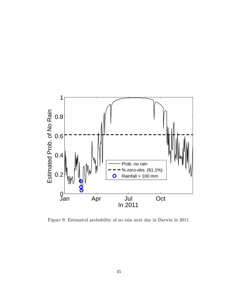
The probability of the next observation being non-zero is given by Fx(ct|t−1e−λt|t−1).
Figure 9 shows the estimated dynamic probability of no rain tomorrow in
2011; compare Figure 5. The small circles mark days with more than 100mm
of rain. Such days roughly coincide with a high probability of rain. As with
the scores, the correlogram of the binary variables, shown in Figure 10, gives
no indication of serial correlation.
[Figure 9 about here.]
[Figure 10 about here.]
5.3 Out-Of-Sample Performance
The out-of-sample period is from 1 January 2016 to 31 August 2016, which
is 244 days. The correlogram of post-sample scores in Figure 11 shows no
serial correlation. The same is true for the binary variables (not shown).
5Tests against time-variation that has not been captured by the model can, in principle,be constructed using score-based (Lagrange multiplier) tests. Such tests have been shownto be very effective; see Harvey (2013, section 2.5), Harvey and Thiele (2016) and Calvoriet al (2016). When the focus of attention is on λ in a location/scale model, score testsdiffer from tests based on the raw residuals; see, for example, HMS (2014, p 95-6). LMtest statistics have not been computed here but the residual correlogram shown here isinformative and re-assuring.
24

The post-sample goodness of fit can be assessed by the predictive likeli-
hood, that is the sum of the logarithms of the log-likelihoods. We can also
look at the ability of the model to forecast the binary outcome of whether or
not it rains tomorrow. The overall forecasting performance may be measured
by the Brier probability score
PS = {Fx(ct|t−1e−λt|t−1)− (1− I(yt > 0)}2; (18)
see Gneiting and Ranjan (2011, p 412). Table 4 gives the average predictive
likelihood and the Brier probability score, computed using a uniform weight-
ing scheme. The associated t-statistics are for comparing one-step ahead
density forecasts. The t-statistics are negative and statistically significantly
showing that the dynamic model specification is preferred.
[Table 4 about here.]
[Figure 11 about here.]
Finally the viability of obtaining multi-step ahead density forecasts by
simulation is illustrated in Figure 12. This shows the median and the 75%
quantile for Darwin obtained at the start of 2016.
[Figure 12 about here.]
25

6 Conclusion
Two ways of constructing a point-mass distribution were considered. One,
which is new, deals with zeroes by shifting a continuous distribution for
non-negative variables to the left and then censoring it at zero. The other
augments the continuous distribution with a binary mechanism for zeroes and
positive observations. In the dynamic case, the scale changes and is driven
by the score. The scale in turn feeds into a mechanism that determines the
degree of censoring or the probability of a zero. The application to daily
rainfall illustrates the use of these models and shows that both are viable.
The censored distribution model appears to be better for the Darwin data
whereas for Cairns the zero-augmented model is superior.
The data are highly seasonal and a large part of the change in scale
is determined by a seasonal pattern that is parsimoniously modeled by a
cubic spline. The seasonal pattern was assumed to be fixed, but for a longer
time series it might be possible to capture a changing seasonal pattern, as
in Proietti and Hillebrand (2017). Ito (2016) shows how dynamics may be
introduced into the seasonal spline. Another unexplored issue concerns the
use the use of periodic models, where parameters are different in different
seasons; see Hipel andMcLeod (1994). The parameters in periodic models are
typically the dynamic parameters, such as φ and κ, but shape parameters may
also change as distributions change with the seasons. For daily data a viable
way of including such effects would be to relate the dynamic and/or shape
26

parameters to the seasonal variation captured by the spline. For example,
we might use a logistic transformation for the autoregressive parameter. We
did not investigate periodic models given our relatively short time series, but
it may be a topic for future research.
The model may be extended by including explanatory variables other than
seasonals. For example, rainfall depends on air pressure and hence predicted
air pressure could be used in conjunction with our models to forecast the
probability of rain and give a distribution of rainfall.
Finally it should be noted that our treatment of dynamics for a censored
distribution has a wide range of applications in economics and finance.
APPENDIX
A Score inequality
The result is proven by noting that the expectation of the score is zero. In
the censored model
E
[∂ ln f(yt)
∂λ
]= Fx(c)
∂ lnFx(c)
∂λ+
∫ ∞c
∂ ln fx∂λ
fxdx = 0,
whereas in the uncensored case
∫ c
0
∂ ln fx∂λ
fxdx+
∫ ∞c
∂ ln fx∂λ
fxdx = 0
27

Thus ∫ c
0
∂ ln fx∂λ
fxdx = Fx(c)∂ lnFx(c)
∂λ
Because the score is monotonically increasing
∂ ln fx(0)
∂λ
∫ c
0
fxdx ≤∫ c
0
∂ ln fx∂λ
fxdx ≤∂ ln fx(c)
∂λ
∫ c
0
fxdx
and (4) follows.
B Expectation and variance of score of a cen-
sored GB2
E∂ ln f(yt)
∂λ= −Fx(c)
υbξc(1− bc)ςβ(zc; ξ, ς)B(ξ, ς)
+
∫ 1
bc
[υ(ξ + ς)bt − υξ]fbdbt
= −υbξc(1− bc)ςB(ξ, ς)
+
∫ 1
bc
[υ(ξ + ς)bt]fbdbt − υξ(1− β(zc; ξ, ς))
= −υbξc(1− bc)ςB(ξ, ς)
+ υ(ξ + ς)B(ξ + 1, ς)
B(ξ, ς)(1− β(zc; ξ + 1, ς))− υξ(1− β(zc; ξ, ς))
= −υbξc(1− bc)ςB(ξ, ς)
+ υξ(1− β(zc; ξ + 1, ς)− υξ(1− β(zc; ξ, ς))
= −υbξc(1− bc)ςB(ξ, ς)
+ υξ(β(zc; ξ, ς)− β(zc; ξ + 1, ς))
28

Note that zc = (ce−λ)υ and bc = zc/(zc + 1). Then, using (26.5.16) in
Abramovitz and Stegun (1964, p 944),
β(zc; ξ, ς)− β(zc; ξ + 1, ς) =1
ξB(ξ, ς)bξc(1− bc)ς .
As regards the variance of the score
E
(∂ ln f(yt)
∂λ
)2=
υ2b2ξc (1− bc)2ςβ(zc; ξ, ς)B2(ξ, ς)
+
∫ 1
bc
[υ(ξ + ς)bt − υξ]2fbdbt
=υ2b2ξc (1− bc)2ςB(zc; ξ, ς)B(ξ, ς)
+ υ2(ξ + ς)2B(ξ + 2, ς)
B(ξ, ς)(1− β(zc; ξ + 2, ς))
−2υ2(ξ + ς)ξB(ξ + 1, ς)
B(ξ, ς)(1− β(zc; ξ + 1, ς)) + υ2ξ2(1− β(zc; ξ, ς))
which then gives (10).
ACKNOWLEDGEMENT
Ryoko Ito thanks Nuffi eld College and the Institute for New Economic
Thinking at the Oxford Martin School of Oxford University for their financial
support.
29

REFERENCES
Abramowitz, M. and I. A. Stegun, (eds.), 1964, Handbook of Mathematical
Functions, New York: Dover Publications Inc.
Ahmad, M. I., Sinclair, C. D. and A. Werritty, 1988, Log-Logistic Flood
Frequency Analysis, Journal of Hydrology, 98, 205—224.
Allik, B., Miller, C., Piovoso, M. J. and R. Zurakowski, 2016, The Tobit
Kalman Filter: An Estimator for Censored Measurements. IEEE Transac-
tions on Control Systems Technology, 24, 365-71.
Bauwens, L., Giot, P., Grammig, J. and D. Veredas, 2004, A Comparison
of Financial Duration Models via Density Forecasts. International Journal
of Forecasting, 20, 589-609.
Blasques, F., Koopman, S. J. and A. Lucas, 2014, Maximum Likelihood
Estimation for Generalized Autoregressive Score Models. Tinbergen Institute
Discussion Paper, TI 2014-029/III, Amsterdam.
Calvori, F., Creal, D.W., Koopman, S.J. and A. Lucas, 2016, Testing
for Parameter Instability in Competing Modeling Frameworks, Journal of
Financial Econometrics (forthcoming).
Creal, D., Koopman, S. J. and A. Lucas, 2011, A Dynamic Multivariate
Heavy-Tailed Model for Time-Varying Volatilities and Correlations, Journal
of Business and Economic Statistics 29, 552-63.
Creal, D., Koopman, S. J. and A. Lucas, 2013, Generalized Autoregressive
Score Models with Applications. Journal of Applied Econometrics, 28, 777-
95.
30

Gneiting, T. and R. Ranjan, 2011, Comparing Density Forecasts using
Threshold- and Quantile-Weighted Scoring Rules. Journal of Business and
Economic Statistics, 29, 411-22.
Hautsch, N., Malec, P. and M. Schienle, 2014, Capturing the Zero: New
Class of Zero-Augmented Distributions and Multiplicative Error Processes,
Journal of Financial Econometrics, 12, 89-121.
Harvey, A.C. , 2013, Dynamic Models for Volatility and Heavy Tails: with
Applications to Financial and Economic Time Series. Econometric Society
Monograph, Cambridge University Press.
Harvey, A.C. and R-J. Lange, 2016, Volatility Modeling with a General-
ized t-Distribution, Journal of Time Series Analysis (forthcoming).
Harvey, A.C. and S. Thiele, 2016, Testing Against Changing Correlation.
Journal of Empirical Finance, 38, 575-89.
Hipel, R. W., and A. I. McLeod, 1994, Time Series Modelling of Water
Resources and Environmental Systems. Developments in Water Science, 45,
Elsevier, Amsterdam.
Ito, R. , 2016, Spline-DCS for Forecasting Trade Volume in High-Frequency
Finance, Cambridge Working Papers in Economics (CWPE1606), University
of Cambridge.
Kleiber, C. and S. Kotz, 2003, Statistical Size Distributions in Economics
and Actuarial Sciences. New York: Wiley.
McDonald, J.B. and W.K. Newey, 1988, Partially Adaptive Estimation of
Regression Models via the Generalized t Distribution, Econometric Theory,
31

4, 428-457.
Park, J. W., Genton, M. G., and Ghosh, S. K., 2007, Censored Time Series
Analysis with Autoregressive Moving Average Models, Canadian Journal of
Statistics, 35, 151—168.
Proietti, T. and E. Hillebrand, 2017, Seasonal Changes in Central Eng-
land Temperatures. Journal of the Royal Statistical Society, Series A (forth-
coming)
Rydberg, T., and N. Shephard, 2003, Dynamics of Trade-by-Trade Price
Movements: Decomposition and Models. Journal of Financial Econometrics
1, 2—25.
Teräsvirta, T. and I. Mellin, 1986, Model Selection Criteria and Model
Selection Tests in Regression Models. Scandinavian Journal of Statistics, 13,
159-171.
Zeger, S. L. and R. Brookmeyer, 1986, Regression Analysis with Censored
Autocorrelated Data, Journal of the American Statistical Association, 81,
722—729.
32

TABLES
Town Fraction of zeroes 75%-quantile Mean Max.
Darwin 0.665 1.8 5.2 367.6
Cairns 0.594 4.0 6.9 381.0Table 1: Sample statistics of rainfall, in millimeters, for the period 1
January 2006 and 31 December 2015.
33

Censor Zero-augmented
α1 = 0 α1 6= 0 δ1 = 0 δ1 6= 0
Darwin AIC 3.175 3.170 3.206 3.172
BIC 3.204 3.199 3.235 3.200
Cairns AIC 3.955 3.951 4.059 3.945
BIC 3.984 3.980 4.088 3.974Table 2 Goodness of fit statistics
34

Location Darwin Cairns
Model Censored Zero-aug.
Estimate S.E. Estimate S.E.
ω 0.43 0.55 0.54 0.13
φ 0.68 0.05 0.59 0.02
κ 0.41 0.06 0.29 0.04
δ0 - - -1.59 0.42
δ1 - - 2.34 0.18
α0 1.51 0.25 - -
α1 -0.38 0.20 - -
ν 0.63 0.09 0.81 0.03
ξ 1.75 0.15 3.12 0.04
η 0.31 0.16 0.44 0.10
η 3.26 2.29
ln L -5767.9 -7183.3Table 3 ML estimates of preferred models with GB2 as in the inverse tail
index parameterization of (6).
35

Town Darwin Cairns
Model Censored Zero-aug.
Static Dynamic Static Dynamic
Predictive likelihood 1.23 1.21 2.15 1.96
t-stat -3.70 -9.39
Brier PS 0.884 0.876 0.86 0.78
t-stat -2.66 -10.28Table 4 Average predictive likelihood and Brier probability scores, together
with the associated t-statistics for comparing one-step ahead density
forecasts.
36

FIGURES
0 20 40 60 80Daily rainfall (mm), January
0
5
10
15
20
25
30
35
His
togr
am
Figure 1: Daily rainfall in Darwin in December. Positive observations onlyarranged in bins of width 1mm
37

0.5 0.5 1.0 1.5 2.0 2.5 3.0 3.5 4.0
2
1
1
2
y
score
Figure 2: Log-logistic score with υ = 2 and c = 0.5.
38

1 0 1 2 3 4 5
0.1
0.2
0.3
0.4
0.5
0.6
0.7
x, y
f(y), f(x)
Figure 3: Log-logistic (thin line) with unit scale and υ = 2. Censored withc = 1 is thick line. Thin dash is censored with scale of 4. Thick dash isdistribution for positive observations for point-mass mixture with π = 0.5.
39

0 100 200 300Days of year
0
10
20
30
40
50
60
Aver
age
daily
rain
fall
(mm
)
Figure 4: Average daily rainfall in Darwin throughout the year, for 1 January2006 to 31 December 2015.
40

0 100 200 300Days of year
0
2
4
6
8
10
Num
ber o
f day
s of
no
rain
Figure 5: Darwin: Number of days in the sample period with no rain.
41

0 20 40 60 80Daily rainfall (mm), November
0
5
10
15
20
25
30
35
His
togr
am
Figure 6: Daily rainfall in Darwin in November. Positive observations onlyarranged in bins of width 1mm
42

0 0.2 0.4 0.6 0.8 10
0.2
0.4
0.6
0.8
1
Standard centered PIT
Empi
rical
CD
F
Figure 7: PITs for Darwin
43

0 100 200 3000.4
0.2
0
0.2
0.4
Lag
Sam
ple
Auto
corr.
of u
95% C.I.
Figure 8: Correlogram of scores from dynamic model fitted to Darwin
44
Jan Apr Jul Oct0
0.2
0.4
0.6
0.8
1
In 2011
Estim
ated
Pro
b. o
f No
Rai
n
Prob. no rain% zeroobs. (61.1%)Rainfall > 100 mm
Figure 9: Estimated probability of no rain next day in Darwin in 2011.
45

0 100 200 3000.4
0.2
0
0.2
0.4
Lag
Sam
ple
Auto
corr.
of v
95% C.I.
Figure 10: Correlogram of binary variables from dynamic model fitted toDarwin
46

0 10 20 300.4
0.2
0
0.2
0.4
Lag
Auto
corr.
of f
orca
st u
95% C.I.
Figure 11: Correlogram of out of sample scores for dynamic model fitted toDarwin
47

Jan Mar Apr Jun AugIn 2016
0
10
20
30
40
50
Mul
tiSt
ep D
ensi
ty F
orec
ast b
y Si
m.
Actual rainfallSim. Density 75%Quant.Sim. Density Median
Figure 12: Multi-step predictive density for Darwin at the start of 2016.
48
Related Documents