Modeling the structure and variability of the southern Benguela upwelling using QuikSCAT wind forcing

Ple

ase

note

that

this

is a

n au

thor

-pro

duce

d P

DF

of a

n ar

ticle

acc

epte

d fo

r pub

licat

ion

follo

win

g pe

er re

view

. The

def

initi

ve p

ublis

her-a

uthe

ntic

ated

ver

sion

is a

vaila

ble

on th

e pu

blis

her W

eb s

ite

1

JOURNAL OF GEOPHYSICAL RESEARCH July 2005; 110(C7) : NIL_1-NIL_18 http://dx.doi.org/10.1029/2004JC002529© 2005 American Geophysical Union An edited version of this paper was published by AGU.

Archimer http://www.ifremer.fr/docelec/Archive Institutionnelle de l’Ifremer

Modeling the structure and variability of the southern Benguela upwelling using QuikSCAT wind forcing

Bruno Blankea, Sabrina Speicha, Abderrahim Bentamyb*, Claude Royb*, Bamol Sowc

aLaboratoire de Physique des Oceans, UMR 6523, Centre National de la Recherche Scientifique/Institut Français de Recherche pour l'Exploitation de la Mer/Université de Bretagne Occidentale, Brest, France bInstitut Français de Recherche pour l'Exploitation de la Mer, Plouzané, France cLaboratoire de Physique de l'Atmosphère Siméon Fongang, Université Cheikh Anta Diop, Dakar, Senegal *: Corresponding author : [email protected] [email protected]

Abstract: The structure and patterns of variability of the southern Benguela coastal upwelling system are investigated with a high-resolution regional model forced by QuikSCAT winds over 1999–2003. The relevance of this global wind product is tested, at first, for the specific nearshore southeast Atlantic; then, the wind products are spatially or temporally degraded from the original 0.5° daily fluxes and are used to diagnose the main scales of the surface dynamical forcing variability. Time resolution appears as a crucial factor in the wind stress to retrieve the patterns of interannual anomalies in sea surface temperatures in a good agreement with independent NASA Pathfinder observations. Various upwelling indices are also calculated in the model to study specific warm or cold coastal events whose circulation schemes are detailed from a Lagrangian interpretation of the model time-varying three-dimensional velocity field. Our study emphasizes the connections established between the Benguela upwelling and the large-scale circulation in relation with, for instance, the Agulhas Current retroflection and associated ring shedding. Keywords: Coastal upwelling, Ai sea interaction, High resolution model

3

1. Introduction

The Benguela system, situated off the west coast of Africa, is one of the four major eastern

boundary upwellings of the World Ocean and spans the countries of Angola, Namibia and South

Africa. It is unique because it is bounded by warm water currents, namely the tropical Angola and

the Indian Ocean Agulhas Current systems at its northern and southern ends, respectively [Shannon

and Nelson, 1996 ; Shillington 1998]. The Agulhas retroflection introduces a high degree of

variability with no equivalent in any other upwelling area ; this results in a net equatorward

movement of heat in the Southeast Atlantic and connects the Benguela Current with the Indo-

Pacific [Lutjeharms, 1996]. The southern part of the Benguela system is located poleward of the

permanent Luderitz upwelling cell off Namibia at around 26°S. Here, like in the other eastern

boundary currents, fisheries are a major activity. They aim at targeting pelagic and demersal

resources found in abundance because of enhanced plankton production driven by intense

movement of surface water away from land together with the subsequent occurrence of cold

nutrient-rich water from the ocean depths [Shannon and Pillar, 1986]. By comparison with the

northern system, the southern Benguela region shelters numerous species, partly because of a higher

regularity in temperature anomalies, salinity and oxygen concentration at the origin of greater

stability and predictability of environmental factors [Shannon et al., 1985].

In the southern Benguela region, the surface currents are generally equatorward with vigorous

upwelling cells, strong and narrow equatorward shelf edge jets (near Cape Town and off Luderitz),

and a poleward undercurrent along the shelf bottom [Nelson and Hutchings, 1983] (see Figure 1).

A year-round upwelling is observed between approximately 15° and 30°S as well as a region of

seasonal upwelling further south [Cole and Villacastin, 2000]. Over the continental shelf, the

spectra of currents show significant peaks of periods ranging from 2.5 to 4 days [Nelson, 1989]

related either to modulations in atmospheric forcing [Jury, 1986] or to coastal trapped waves

traveling poleward, with periods of 3 to 8 days, from Walvis Bay in Namibia (20°S) to Port

Elizabeth (25.6°E) on the east coast of South Africa [Brundrit et al., 1987 ; Schumann and Brink,

4

1990]. These waves result in a net poleward flow of about 6 cm/s [Nelson, 1989], enhanced or

reduced upwelling and larger sea level changes than those simply inferred from wind. Nevertheless,

the areas along the west coast of southern Africa, where the strongest winds are the southerly ones,

are also those where upwelling is the most pronounced ; atmospheric variability is, to a large extent,

responsible for the occurrence of cold and warm events [Shannon et al., 1986 ; Shannon and

Nelson, 1996 ; Roy et al., 2001 ; Hardman-Mountford et al., 2003].

It is worth underlining that the longest series of reliable data for the Benguela region deals

with sea surface temperature (SST). Other oceanographic records (physical, chemical or biological

parameters) are either shorter or scattered in space and time. Therefore, our understanding of

interannual variability in the Benguela upwelling comes mainly from case studies of extreme, or

episodic, environmental warm, or cold, events, and among them especially from those responsible

for successive collapses, recoveries and switches in species dominance [Shannon et al., 1992]. The

background knowledge needed to understand, in particular, the differences in the way the northern,

central and southern parts of the Benguela upwelling system function requires the development of

viable integrative environmental mechanisms for the region as a whole, i.e., at the ecosystem level

[Hutchings et al., 1995]. From a management point of view, these changes in environmental events

as well as their impacts on the southern Benguela upwelling need to be predicted. The unique

character of the region necessitates special attention as this area borders the global ocean heat

“conveyer belt” linking the Pacific, Indian and Atlantic Oceans [Gordon, 1986 ; Rintoul, 1991] with

a potential impact of local marine environmental processes on world climate and vice versa.

To investigate the dynamics of marine resources in the Benguela region, a suite of models

taking advantage of the knowledge gained during the Benguela Ecology Program [Payne et al.,

1992 ; Pillar et al., 1998] has been designed and implemented [Fréon, 2000]. One of them is a

high-resolution regional model of the southern Benguela circulation [Penven et al., 2001a]. In this

study our aim is to use it to diagnose in the surface wind stress the scales of variability relevant to

the occurrence of anomalous warm, or cold, events. Our second objective is to build model-based

5

dynamical-upwelling indices aimed at characterizing the intensity and spatial extent of the

upwelling process. Then, we will propose circulation schemes for specific anomalous events and we

will relate them to the surrounding large-scale circulation. It is worth noting that, over more than

two decades, rather extensive investigations about upwelling processes over the Benguela shelf

were based on cruise- and mooring-data [see for instance Nelson and Hutchings, 1983] ; in other

respects, modeling studies can focus on the context of interactions between open ocean structures in

relation, for instance, with the Indian-Atlantic connection and smaller scales related to the

continental shelf and the upwelling itself. They will provide the background knowledge needed to

understand the impact of anomalous oceanographic events on transport processes linking the

spawning and nursery grounds of the southern Benguela upwelling system. The coastal jet flowing

along the Cape Peninsula is, indeed, another major oceanographic feature of the southern Benguela

region : it shows strong, semi-permanent, surface equatorward velocities ranging from 25 to

75 cm/s [Bang and Andrews, 1974 ; Gordon et al., 1995]. Moreover, this jet acts as the major

conveyor belt between the distant fish spawning areas on the Agulhas Bank and the nursery area

located within the upwelling region, at the north of Cape Columbine ; variability in the intensity

and direction of this flow is thought to be a major contributor in the success of fish recruitment.

To address these issues, our paper is organized as follows : section 2 introduces briefly the

numerical model and the main simulation parameters before discussing some issues in QuikSCAT

wind data. Section 3 presents the model sensitivity to changes in the space or time resolution of the

wind stress through degradation of the nominal QuikSCAT resolution. Section 4 deals with the

calculation of several dynamic upwelling indices and relates them to variability in the surface wind

stress and SST. The embedding of the coastal upwelling flow within the larger scales of the

Southeast Atlantic circulation is studied in section 5 with the calculation of circulation schemes in

relation with specific warm and cold events. Our conclusion is drawn in section 6.

2. Modeling Approach

6

a) The ocean model

The hydrodynamic code used is the Regional Ocean Modeling System (ROMS) [Haidvogel et

al., 2000 ; Marchesiello et al., 2001] ; the configuration used in this study was described in detail

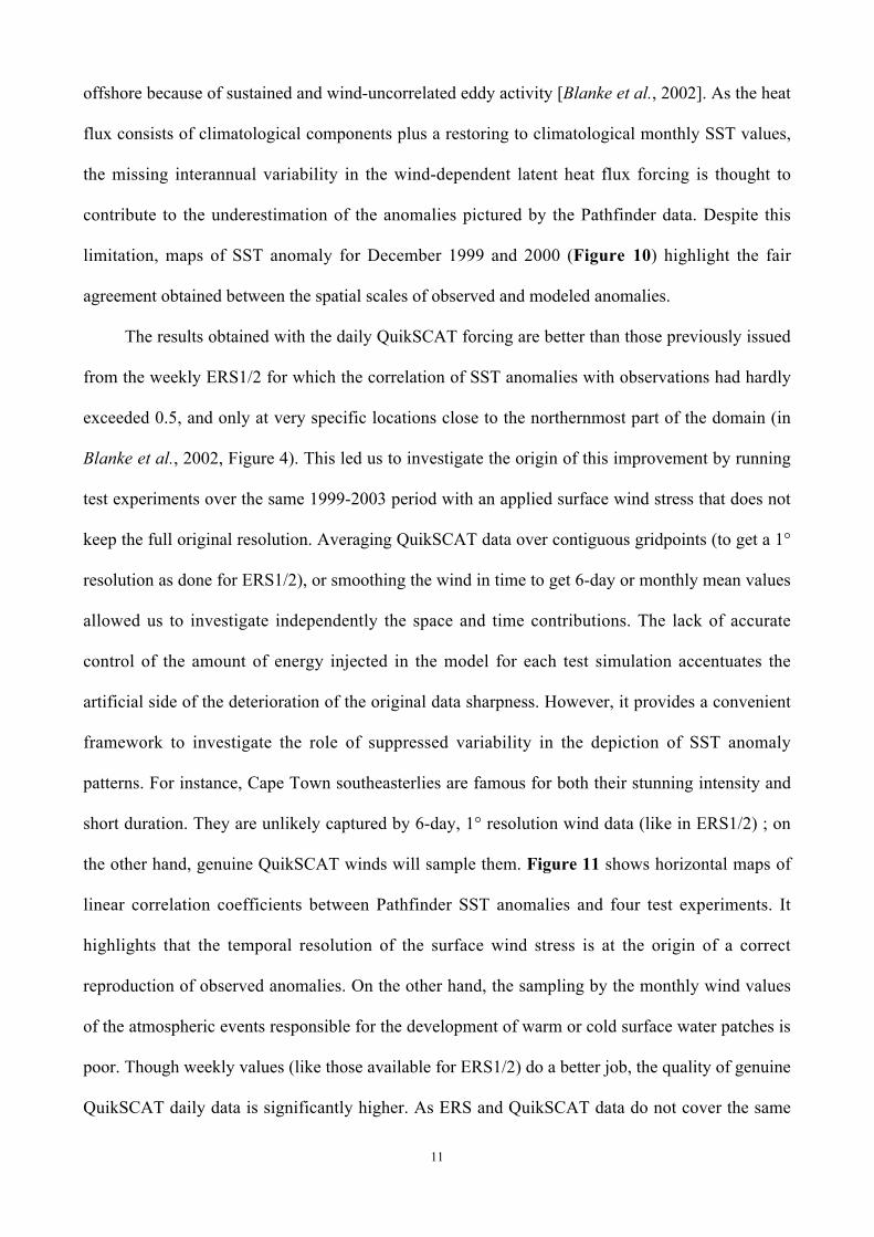
by Penven et al. [2001a] and Blanke et al. [2002]. The domain of study covers the southwestern

corner of Africa from 40°S to 28°S and from 10°E to 24°E ; resolution ranges from 9 km at the

coast to 16 km offshore (Figure 1) with 20 terrain-following levels that keep a high resolution near

the surface. Realistic topographic features are slightly smoothed to ensure stable and accurate

simulations [Haidvogel et al., 2000]. Surface wind stress apart, the model is forced with

climatological fluxes : heat and salinity fluxes from the Comprehensive Ocean–Atmosphere Data

Set (COADS) ocean surface monthly climatology [Da Silva et al., 1994] at the surface, and

seasonal time-averaged outputs of the AGAPE basin-scale ocean model [Biastoch and Krauß,

1999] at the three lateral boundaries facing the open ocean with an implicit active radiative

boundary scheme [Marchesiello et al., 2001]. In addition, a one-way radiative nesting scheme

[Flather, 1976] is adopted for the barotropic contribution. All subsequent analyses are developed

from two-day archives that sample appropriately the simulated variability.

A study by Blanke et al. [2002] demonstrated that the model forced by the weekly

1°×1°–resolution ERS1/2 wind stress gives a reasonably good representation of coastal upwelling

variability. However, some obvious disagreements between modeled and observed SST anomalies

were likely attributable to an insufficient wind resolution, both in space and time. The recent

availability, at IFREMER, of a four-year wind stress time series from the QuikSCAT satellite radar

scatterometer [Bentamy et al., 2002] encouraged us to pursue our progressive modeling approach of

interannual SST fluctuations by incorporating external variability with a daily and

0.5°×0.5°–resolution in the surface wind stress.

b) Surface wind stress sampling

7

QuikSCAT scatterometer swath is 1800 km, and its orbit is about 110 min. Hence,

scatterometer wind estimates can be close in space, but widely separated in time. Furthermore at a

given location, wind variability can be high during few hours. On average and over our area of

interest, two wind observations are expected at each grid point (0.5°×0.5°) on a daily basis.

However, on some particular days, QuikSCAT swath would not cover some sub-areas, and this

would result in a poor wind sampling. Even though the kriging method uses a structure function of

wind variables [IFREMER/CERSAT, 2002], it is necessary to investigate the impact of the number

and of the spatial and temporal distribution of the observations that are used to estimate the wind at

each gridpoint. As already done for ERS1/2 wind estimates [Bentamy et al., 1996], the question

brings in the impact of scatterometer sampling on the method accuracy and retrieval of highly

variable events by the objective analysis.

A good way to address the aliasing problem is to simulate scatterometer wind sampling from

regular surface winds considered as the “ground truth”, and then to compare the resultant wind field

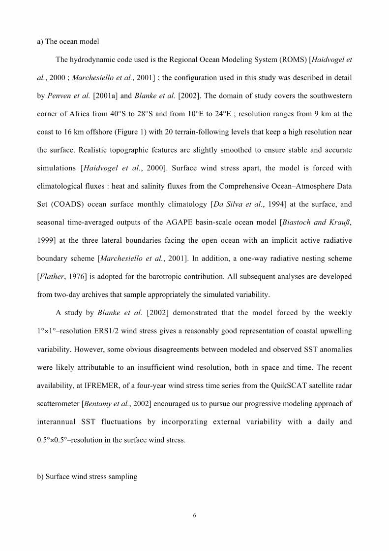
with the original one. We thus chose to use the European Center for Medium-Range Weather

Forecasts (ECMWF) surface wind analysis ; its spatial resolution is 1.125°×1.125° in longitude and

latitude and the analysis is made at synoptic times (00 h, 06 h, 12 h, 18 h). At each scatterometer

cell, ECMWF wind data are linearly interpolated in time and space. The former are called the

simulated scatterometer data, and denoted hereafter as Simu_QSCAT ; they are used to generate a

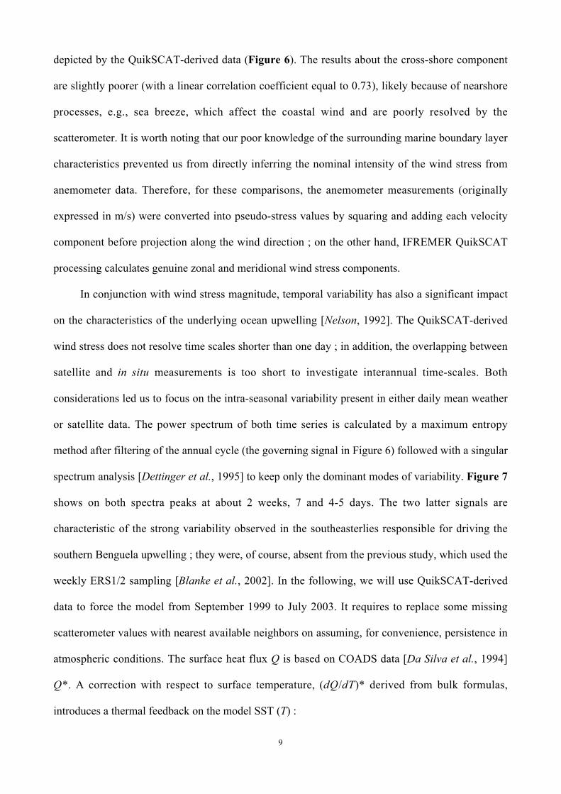
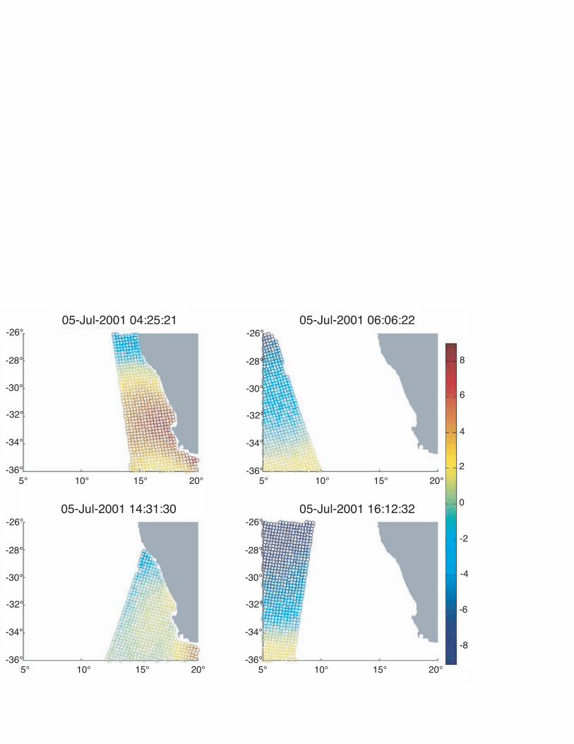
regular wind field through the kriging approach. For instance, Figures 2 and 3 show the four wind

analyses for a specific day, 5 July 2001, and the corresponding Simu_QSCAT, respectively ; they

illustrate the main shortcoming of the scatterometer wind-sampling scheme. Indeed, the eastern and

western areas are well sampled, whereas the central area is desert, e.g., between 10°E and 15°E, and

such cases account for about 30% of the total QuikSCAT wind observations over the Benguela

upwelling system. It is worth also noticing that the wind variability, especially in the southeast

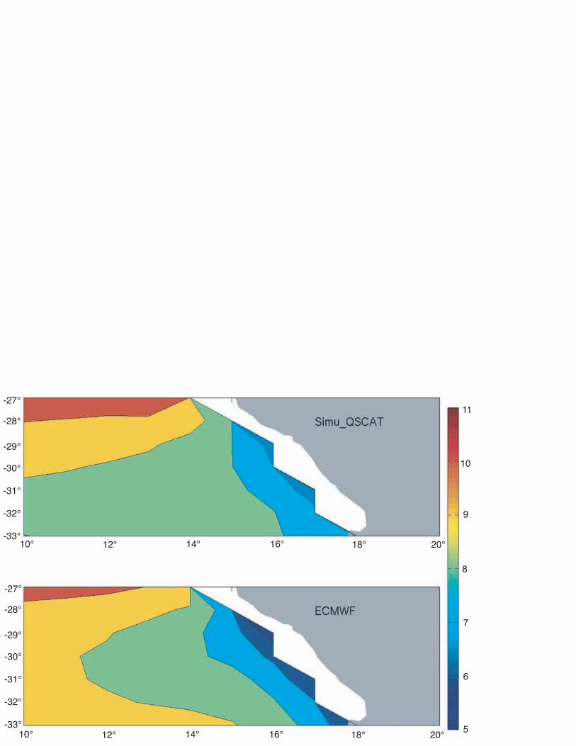
region, decreases from 9 to 5 m/s within 10 hours. Figure 4 (top panel) depicts the daily wind fields

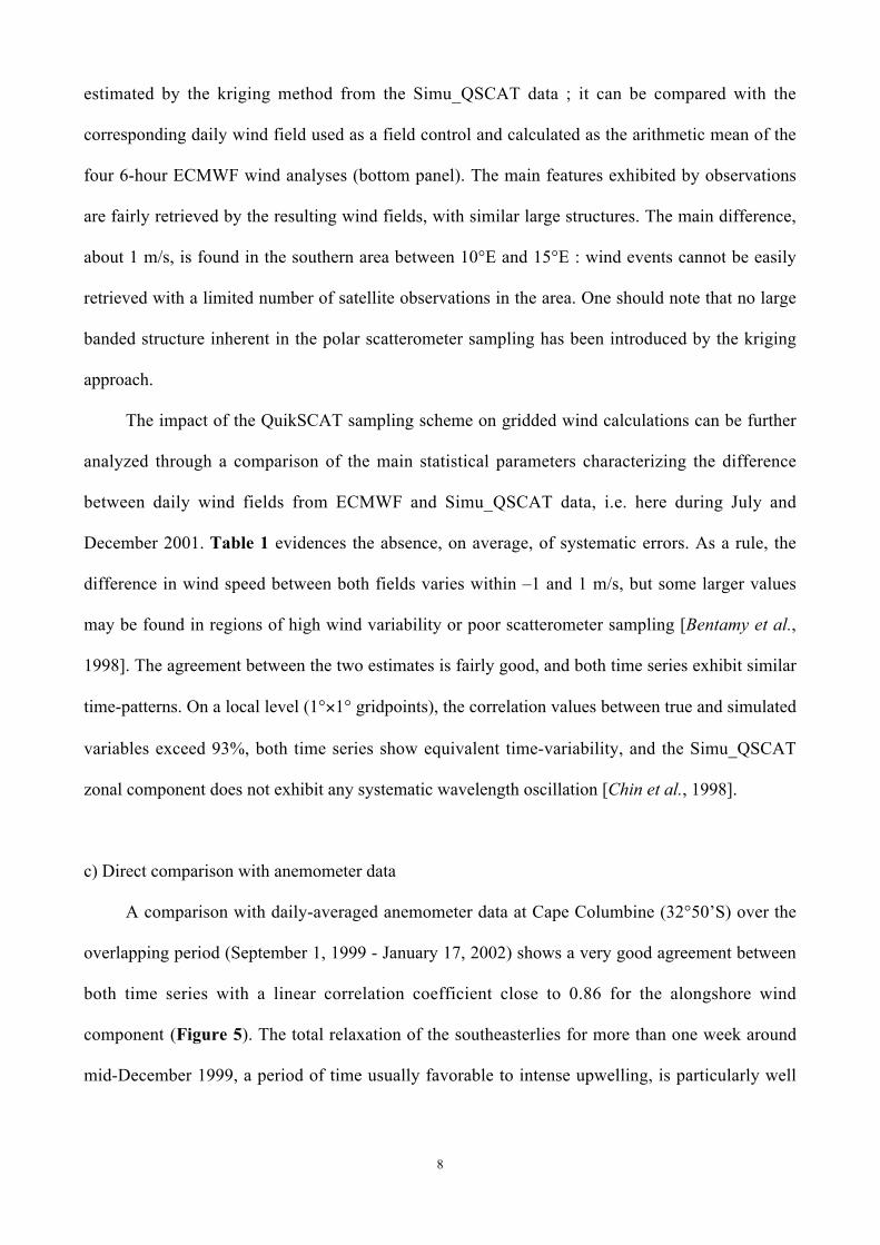
8

estimated by the kriging method from the Simu_QSCAT data ; it can be compared with the

corresponding daily wind field used as a field control and calculated as the arithmetic mean of the

four 6-hour ECMWF wind analyses (bottom panel). The main features exhibited by observations

are fairly retrieved by the resulting wind fields, with similar large structures. The main difference,

about 1 m/s, is found in the southern area between 10°E and 15°E : wind events cannot be easily

retrieved with a limited number of satellite observations in the area. One should note that no large

banded structure inherent in the polar scatterometer sampling has been introduced by the kriging

approach.

The impact of the QuikSCAT sampling scheme on gridded wind calculations can be further

analyzed through a comparison of the main statistical parameters characterizing the difference

between daily wind fields from ECMWF and Simu_QSCAT data, i.e. here during July and

December 2001. Table 1 evidences the absence, on average, of systematic errors. As a rule, the

difference in wind speed between both fields varies within –1 and 1 m/s, but some larger values

may be found in regions of high wind variability or poor scatterometer sampling [Bentamy et al.,

1998]. The agreement between the two estimates is fairly good, and both time series exhibit similar

time-patterns. On a local level (1°×1° gridpoints), the correlation values between true and simulated

variables exceed 93%, both time series show equivalent time-variability, and the Simu_QSCAT

zonal component does not exhibit any systematic wavelength oscillation [Chin et al., 1998].

c) Direct comparison with anemometer data

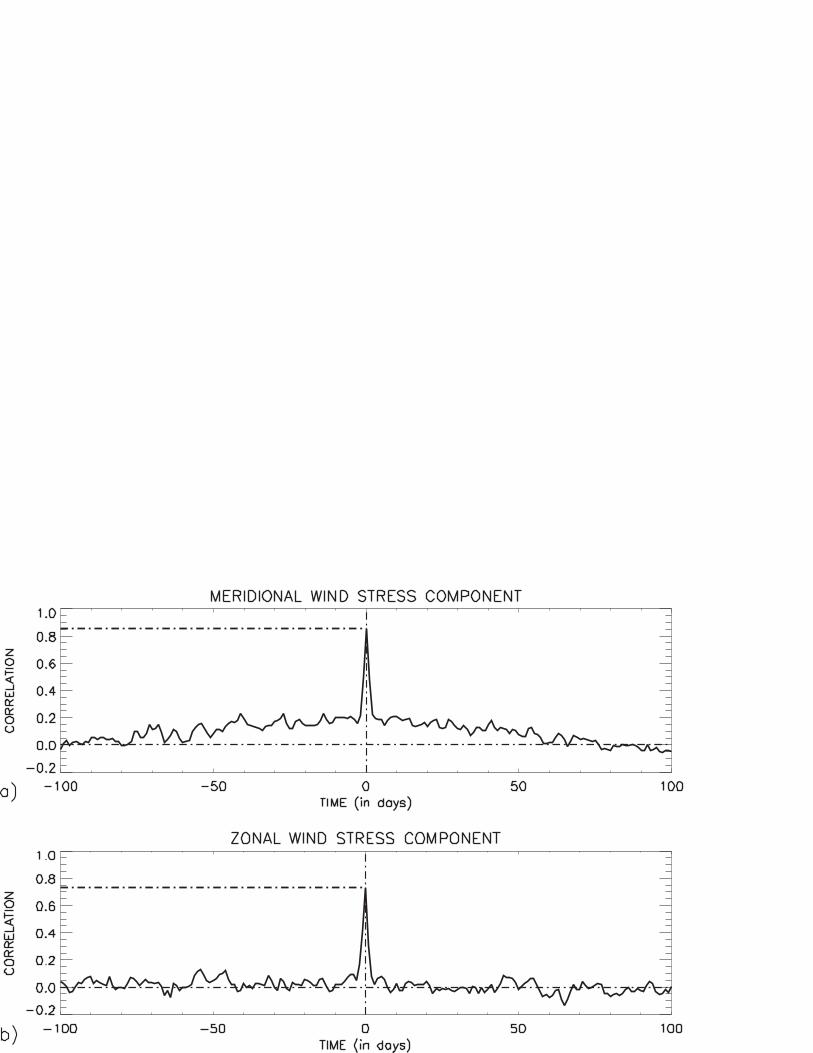
A comparison with daily-averaged anemometer data at Cape Columbine (32°50’S) over the

overlapping period (September 1, 1999 - January 17, 2002) shows a very good agreement between

both time series with a linear correlation coefficient close to 0.86 for the alongshore wind

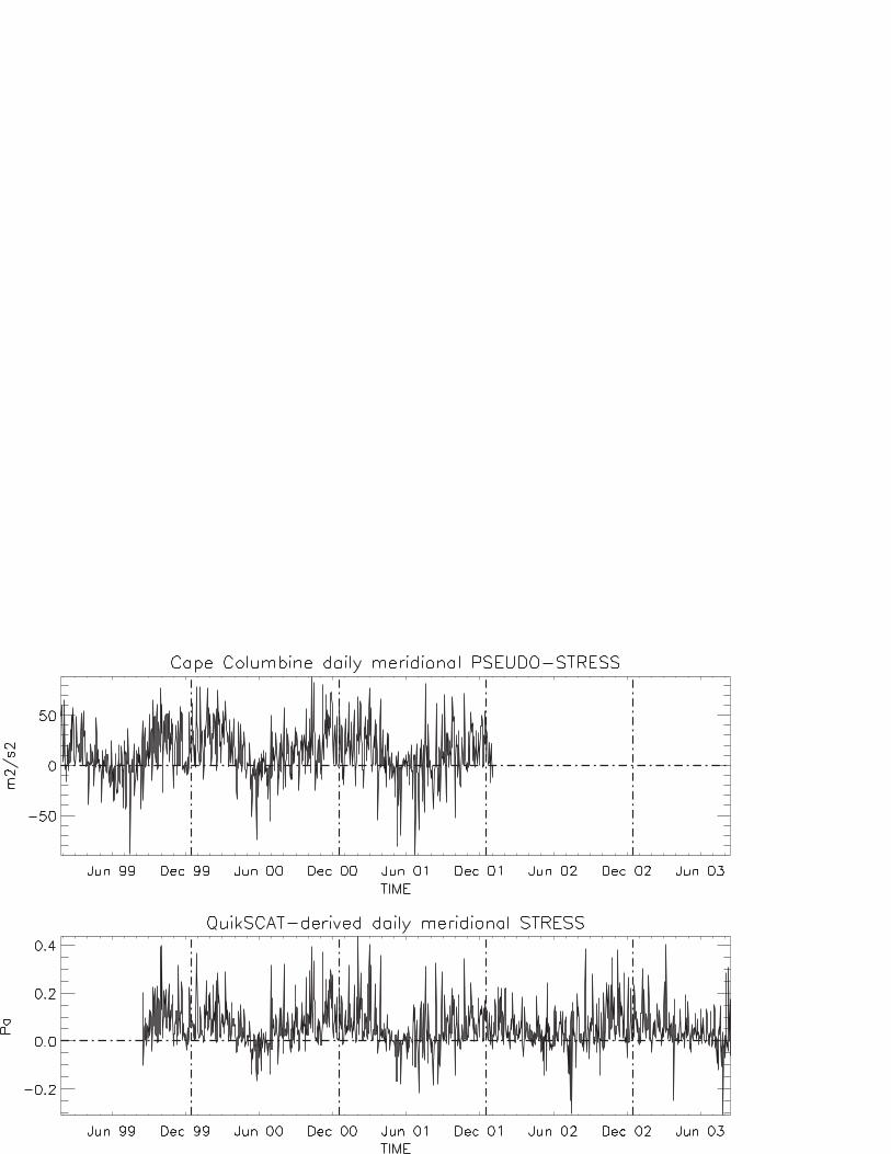
component (Figure 5). The total relaxation of the southeasterlies for more than one week around

mid-December 1999, a period of time usually favorable to intense upwelling, is particularly well

9

depicted by the QuikSCAT-derived data (Figure 6). The results about the cross-shore component

are slightly poorer (with a linear correlation coefficient equal to 0.73), likely because of nearshore

processes, e.g., sea breeze, which affect the coastal wind and are poorly resolved by the

scatterometer. It is worth noting that our poor knowledge of the surrounding marine boundary layer

characteristics prevented us from directly inferring the nominal intensity of the wind stress from

anemometer data. Therefore, for these comparisons, the anemometer measurements (originally

expressed in m/s) were converted into pseudo-stress values by squaring and adding each velocity

component before projection along the wind direction ; on the other hand, IFREMER QuikSCAT

processing calculates genuine zonal and meridional wind stress components.

In conjunction with wind stress magnitude, temporal variability has also a significant impact

on the characteristics of the underlying ocean upwelling [Nelson, 1992]. The QuikSCAT-derived

wind stress does not resolve time scales shorter than one day ; in addition, the overlapping between

satellite and in situ measurements is too short to investigate interannual time-scales. Both

considerations led us to focus on the intra-seasonal variability present in either daily mean weather

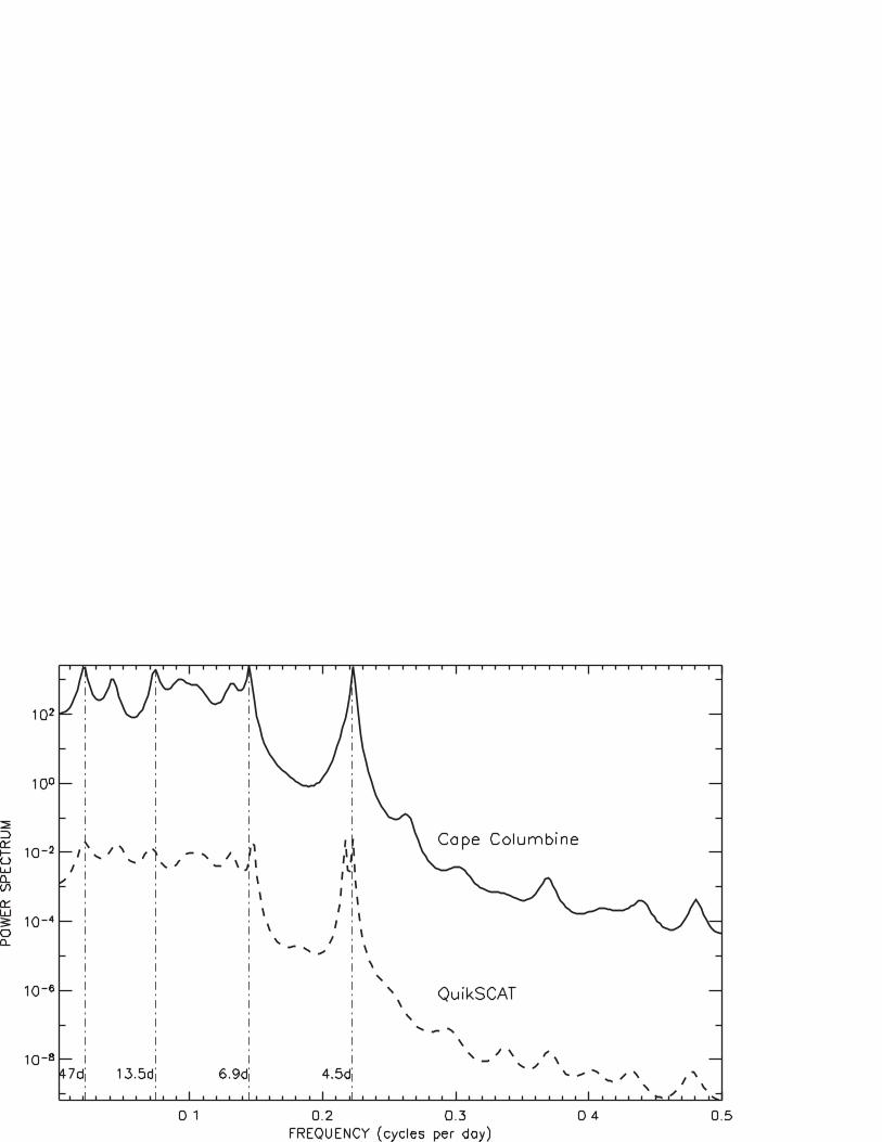
or satellite data. The power spectrum of both time series is calculated by a maximum entropy

method after filtering of the annual cycle (the governing signal in Figure 6) followed with a singular

spectrum analysis [Dettinger et al., 1995] to keep only the dominant modes of variability. Figure 7

shows on both spectra peaks at about 2 weeks, 7 and 4-5 days. The two latter signals are

characteristic of the strong variability observed in the southeasterlies responsible for driving the

southern Benguela upwelling ; they were, of course, absent from the previous study, which used the

weekly ERS1/2 sampling [Blanke et al., 2002]. In the following, we will use QuikSCAT-derived

data to force the model from September 1999 to July 2003. It requires to replace some missing

scatterometer values with nearest available neighbors on assuming, for convenience, persistence in

atmospheric conditions. The surface heat flux Q is based on COADS data [Da Silva et al., 1994]

Q*. A correction with respect to surface temperature, (dQ/dT)* derived from bulk formulas,

introduces a thermal feedback on the model SST (T) :

10

€

Q =Q* +dQdT

*T −T*( ) (1)

where T* is a monthly climatology based on Pathfinder SST timeseries. Finally, the outcome of a

prior 8-year integration with ERS1/2 winds (1991-1999) is used as an initial state for the model.

3. Sensitivity to wind stress resolution

The model displays a rich coastal mesoscale activity with no identical repetition from year to

year because of the variable surface wind stress conditions, intrinsic random eddy and filament

formation [Penven et al., 2001a ; 2001b ; Blanke et al., 2002]. The forcing of the model with

climatological SST and heat flux information allows us to compare objectively simulated and

observed interannual SST anomalies and define a valuable test bench for assessment of the degree

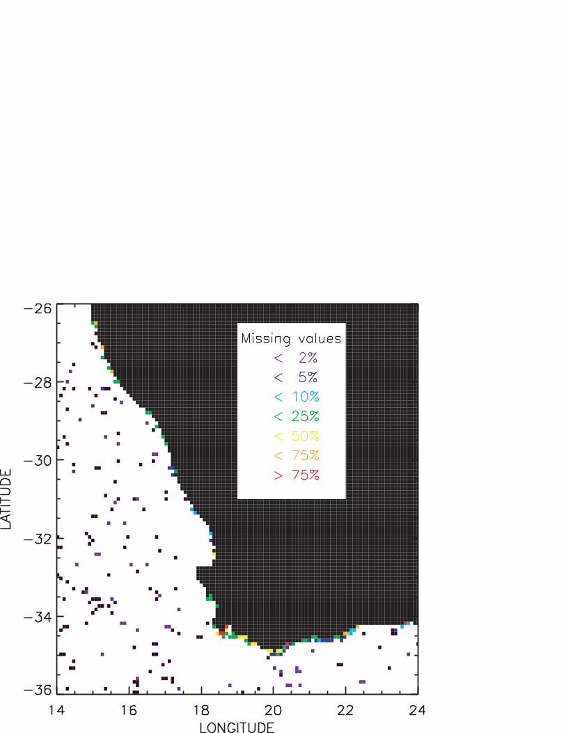
of realism of numerical simulations. We calculated Pathfinder interannual SST anomalies from

nominal monthly 9 km values over 1985-2002. This monthly product presents a limited number of

missing values (due to cloudy pixels in the original satellite data) (Figure 8). It allows an easy

calculation of climatological monthly maps (those used in the model heat flux formulation, i.e., T*

in Equation 1), from which the monthly SST anomalies are derived with no degradation of the

original Pathfinder 9 km resolution. A four-step process is used for the model. At each gridpoint,

we first smooth the SST time series with a 30-day moving averaging window. Then, we compute a

mean seasonal cycle by overlapping and averaging all successive years of the smoothed time series.

Anomalies are diagnosed from differences between the original time series and the mean seasonal

cycle. Monthly anomalies are finally computed by averaging the anomalies over monthly time

periods.

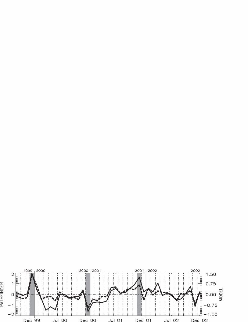
Figure 9 depicts observed and modeled time series of the SST anomalies averaged over the

continental shelf of the southern Benguela upwelling region for depths shallower than 200 m. A

direct response of the model and real ocean to wind variability explains the very fair agreement

between modeled and observed SST anomalies over the shelf ; the correlation is much lower

11

offshore because of sustained and wind-uncorrelated eddy activity [Blanke et al., 2002]. As the heat

flux consists of climatological components plus a restoring to climatological monthly SST values,

the missing interannual variability in the wind-dependent latent heat flux forcing is thought to

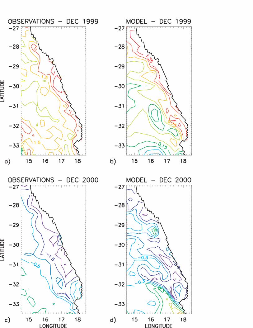
contribute to the underestimation of the anomalies pictured by the Pathfinder data. Despite this

limitation, maps of SST anomaly for December 1999 and 2000 (Figure 10) highlight the fair

agreement obtained between the spatial scales of observed and modeled anomalies.

The results obtained with the daily QuikSCAT forcing are better than those previously issued

from the weekly ERS1/2 for which the correlation of SST anomalies with observations had hardly

exceeded 0.5, and only at very specific locations close to the northernmost part of the domain (in

Blanke et al., 2002, Figure 4). This led us to investigate the origin of this improvement by running

test experiments over the same 1999-2003 period with an applied surface wind stress that does not

keep the full original resolution. Averaging QuikSCAT data over contiguous gridpoints (to get a 1°

resolution as done for ERS1/2), or smoothing the wind in time to get 6-day or monthly mean values

allowed us to investigate independently the space and time contributions. The lack of accurate

control of the amount of energy injected in the model for each test simulation accentuates the

artificial side of the deterioration of the original data sharpness. However, it provides a convenient

framework to investigate the role of suppressed variability in the depiction of SST anomaly

patterns. For instance, Cape Town southeasterlies are famous for both their stunning intensity and

short duration. They are unlikely captured by 6-day, 1° resolution wind data (like in ERS1/2) ; on

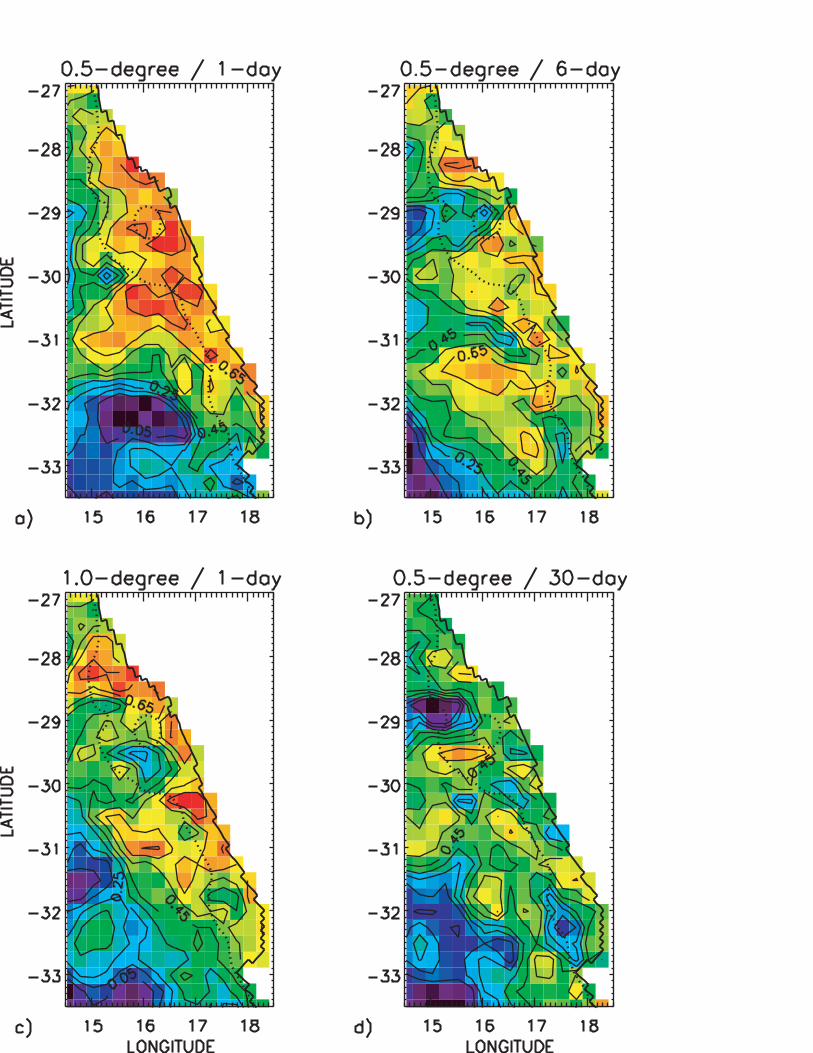
the other hand, genuine QuikSCAT winds will sample them. Figure 11 shows horizontal maps of

linear correlation coefficients between Pathfinder SST anomalies and four test experiments. It

highlights that the temporal resolution of the surface wind stress is at the origin of a correct

reproduction of observed anomalies. On the other hand, the sampling by the monthly wind values

of the atmospheric events responsible for the development of warm or cold surface water patches is

poor. Though weekly values (like those available for ERS1/2) do a better job, the quality of genuine

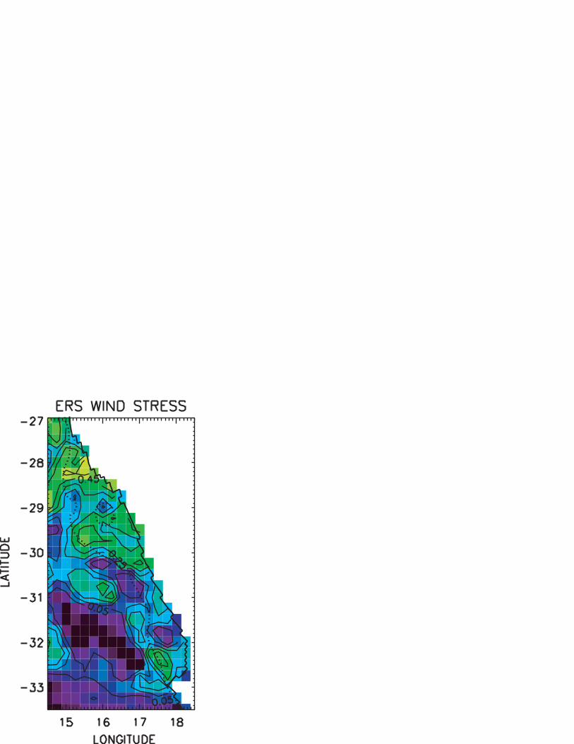
QuikSCAT daily data is significantly higher. As ERS and QuikSCAT data do not cover the same

12

period of time, Figure 12 shows an indirect comparison between both products by computing a

correlation map between Pathfinder SST anomalies and anomalies from the ERS-based experiment

analyzed in a former study [Blanke et al., 2002]. The calculations are done as above over a similar

period of time, but shifted by three years (1996-2000), which still includes the warm event of

December 1999. The spatial resolution of the wind stress looks less decisive, maybe because of the

inclusion in the full resolution QuikSCAT data of some spatial smoothing that softens the effect of

an additional degradation to a 1°×1° product (see section 1b).

According to Roy et al. [2001], whose approach was based on hourly anemometer data,

upwelling events may be defined as periods characterized by uninterrupted northward wind. In

compliance with this approach, we integrate upwelling-favorable winds over time till reaching a

period of unfavorable wind, and then the integration is reset to zero. Each upwelling event is

characterized by its duration (in days) and by the total accumulation of divergence at its end.

Table 2 sums up the results we obtain for the nominal QuikSCAT wind stress and for degraded

products after time and space filtering. To allow comparison with the study by Roy et al. [2001]

who identified a dozen of events for the period extending from 1 November 1999 to 30 April 2000,

let us define as unfavorable upwelling periods the days showing either southward or northward

wind stress below a given threshold τmin, and limit our identification to episodes longer than 3 days.

The value of τmin must be adjusted for each resolution to make sure that, for instance, the warm

episode of December 1999 is always considered as an upwelling-unfavorable period. The

calculations are done with the average value of the wind over the shelf. As expected, the wind stress

resolution causes no significant changes in the total amount of divergence accounted by upwelling

events. The differences are attributable to the non-linearity of the criteria used for the definition of

upwelling episodes. On the other hand, the total number of episodes is very sensitive to the time

resolution of the alongshore wind stress. Daily winds lead to about a hundred of episodes over three

years and a half ; this frequency is comparable with the one obtained by Roy et al. [2001]. Extreme

13

results are, of course, obtained for monthly wind values : upwelling episodes match sometimes the

full upwelling season in the southern Benguela region (roughly from October to March) because

unfavorable wind periods only happen, on a monthly average basis, in April-May. The longest

upwelling episode obtained with the nominal QuikSCAT resolution does not exceed 28 days, and

corresponds to the cold event of December 2000. This episode is also the longest one obtained with

six-day averaged winds, but it lasts much more than one month since it only ends in mid-March

2001. As a rule, six-day averaged winds provide no evidence of the sporadic nature of upwelling

events as they overestimate persistence in wind intensity. On the other hand, this diagnostic

corroborates the weak sensitivity of our modeling results to degradation in the spatial resolution of

the QuikSCAT-derived data.

One should note that correlation maps highlight some skill of the model over a region that

extends slightly beyond the continental shelf. They also present irregular patterns and the upwelling

occurs over a region broader than just the narrow coastal strip, because the offshore Ekman

transport is not a simple uniform flux along the eastern boundary, but occurs rather in jets like in

other eastern-boundary upwelling systems [Marchesiello et al., 2003]. The expansion of the

anomalies out of the shelf area and the increase with the distance to the shelf of the contrasts

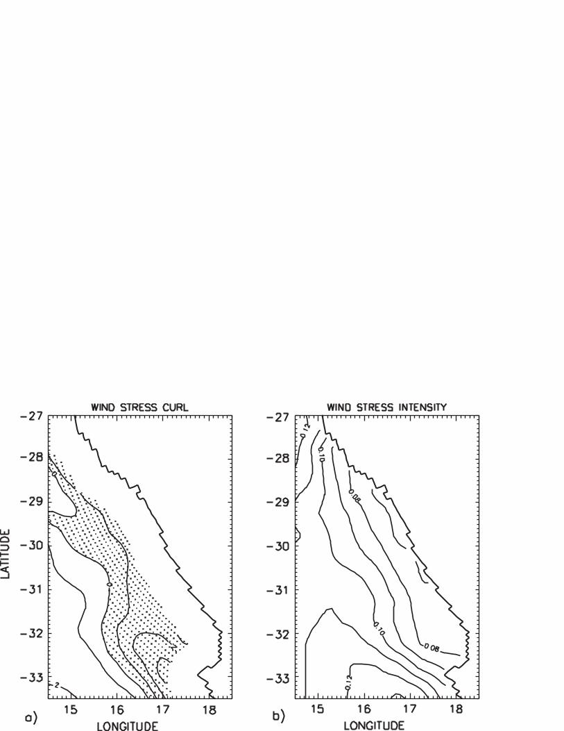
between observed and modeled signals are both worth being noted. One explanation is the negative

wind stress curl (Figure 13) associated with the topographically steered winds and at the origin of

an upwelling zone broader than the one produced by a strictly uniform wind with an equatorward

component. The curl is, here, calculated with the average of daily QuikSCAT wind stress values

over the months of December and January of years 1999 to 2003, and it compares well with the

map established by Bakun and Nelson [1991] and derived from in situ ship measurements.

4. Upwelling indices

a) Meridional structure of the nearshore upwelling

14

Variability in surface wind stress is expected to govern the fluctuations of the upwelling

process, and thus to have a direct impact on the SST field. Upwelling indices are usually based on

wind data or SST ones. These indices are just proxies of the actual process leading to the lift of

deep water onto the shelf, either as a direct compensation for offshore Ekman transport at the

coastline, or as the ocean dynamical response to a negative surface wind stress curl (in the southern

hemisphere). Hydrodynamic models provide an opportunity to directly assess the upwelling process

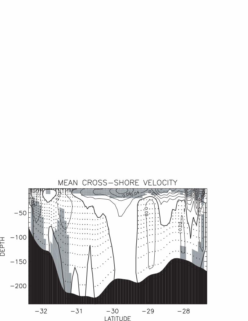
through the use of the simulated, complex three-dimensional velocity field. Figure 14 depicts the

time mean cross-shore velocity (counted positive for offshore movements) close to the shelf edge.

The vertical inspection of the mean flow shows that the southernmost area around St Helena Bay is

mostly associated with coastward movements, whereas the circulation further north shows a clearer

contrast between surface-expelled and subsurface-upwelled waters. This difference fits the view of

mesoscale structures transmitted northward from the retroflection area of the Agulhas Current,

flowing up the continental slope in its southernmost portion and interacting with the upwelling

circulation before attenuation over the shelf and export by Ekman divergence. The next section will

focus on these large-scale connections and more specifically the embedding of the shelf circulation

within the larger scales of the southern Benguela. The shaded areas in Figure 14 evidence the linear

correlation coefficient between local velocity and surface alongshore wind variations. As expected,

the surface Ekman flow varies in close phase with the wind. The deeper flow that feeds the

upwelling is far less structured ; moreover, the position of shoreward currents shows more

numerous time fluctuations and poor correlation with wind, even though the integrated flow

balances exactly the full surface Ekman flow.

Notwithstanding their differences in spatial structure, the expelled surface flow and the

upwelled waters share common properties in magnitude conveniently addressed by upwelling

indices. We choose to focus on two indicators : the former is aimed at characterizing the intensity of

the upwelling in the inner-shelf region, whereas the latter is designed to address, on a broader scale,

the spatial influence of the upwelling process. These indicators provide an integrated vision of the

15

upwelling system by freeing from the meridional variability discussed above. Such indices are

easily comparable to other integrated quantities whose geographical distribution is poorly known

like, for instance, the supply of nutrients over the shelf. Recent major anomalous events for the

southern Benguela include December 1999 and March 2000 [Roy et al., 2001] as well as December

2000 and November 2001 (see Figure 9). As the simulation forced by QuikSCAT-derived wind

stress showed some obvious ability to reproduce this variability, we use the model velocity field to

investigate the magnitude of the upwelling associated with these anomalies.

b) Nearshore upwelling intensity : Shelf overturning

Let us focus, first, on the inner part of the western shelf by building a streamfunction in a

vertical plane to take advantage of the bay-shape aspect of the western coast between 27°S and

33°S (see Figure 1). The net volume transport across the edge of a fixed subdomain with neither

internal source nor sink of mass is virtually zero like, for instance, along the blue line drawn in

Figure 1. The integration along this line of the cross-shore and vertical transport components

following the model alongshore coordinate, j, provides, for each time step, a two-dimensional

transport field (UU, WW) :

€

UU i,k( ) = U(i, j,k)j∑ (2)

€

WW i,k( ) = W (i, j,k)j∑ (3)

where i, j, and k are the model coordinates, U and W are the model cross-shore and vertical

transports, respectively. At any time, this field is non-divergent as both fulcra of the integration are

located on land ; it can be expressed as a streamfunction ψ :

€

UU i,k( ) = δkψ i,k( ) (4)

€

WW i,k( ) = −δiψ i,k( ) (5)

Let us choose the reference (ψ = 0) so that ψ > 0 in standard upwelling conditions (i.e., a

counterclockwise circulation in a cross-shore/depth plane with east to the right hand side).

16

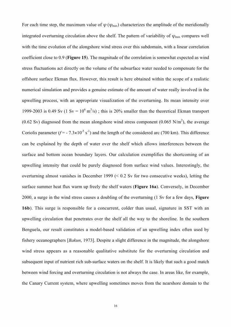
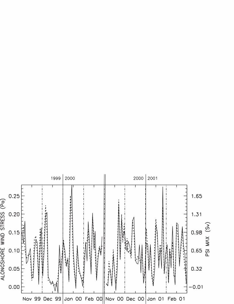
For each time step, the maximum value of ψ (ψmax) characterizes the amplitude of the meridionally

integrated overturning circulation above the shelf. The pattern of variability of ψmax compares well

with the time evolution of the alongshore wind stress over this subdomain, with a linear correlation

coefficient close to 0.9 (Figure 15). The magnitude of the correlation is somewhat expected as wind

stress fluctuations act directly on the volume of the subsurface water needed to compensate for the

offshore surface Ekman flux. However, this result is here obtained within the scope of a realistic

numerical simulation and provides a genuine estimate of the amount of water really involved in the

upwelling process, with an appropriate visualization of the overturning. Its mean intensity over

1999-2003 is 0.49 Sv (1 Sv = 106 m3/s) ; this is 20% smaller than the theoretical Ekman transport

(0.62 Sv) diagnosed from the mean alongshore wind stress component (0.065 N/m2), the average

Coriolis parameter (f = - 7.3×10-5 s-1) and the length of the considered arc (700 km). This difference

can be explained by the depth of water over the shelf which allows interferences between the

surface and bottom ocean boundary layers. Our calculation exemplifies the shortcoming of an

upwelling intensity that could be purely diagnosed from surface wind values. Interestingly, the

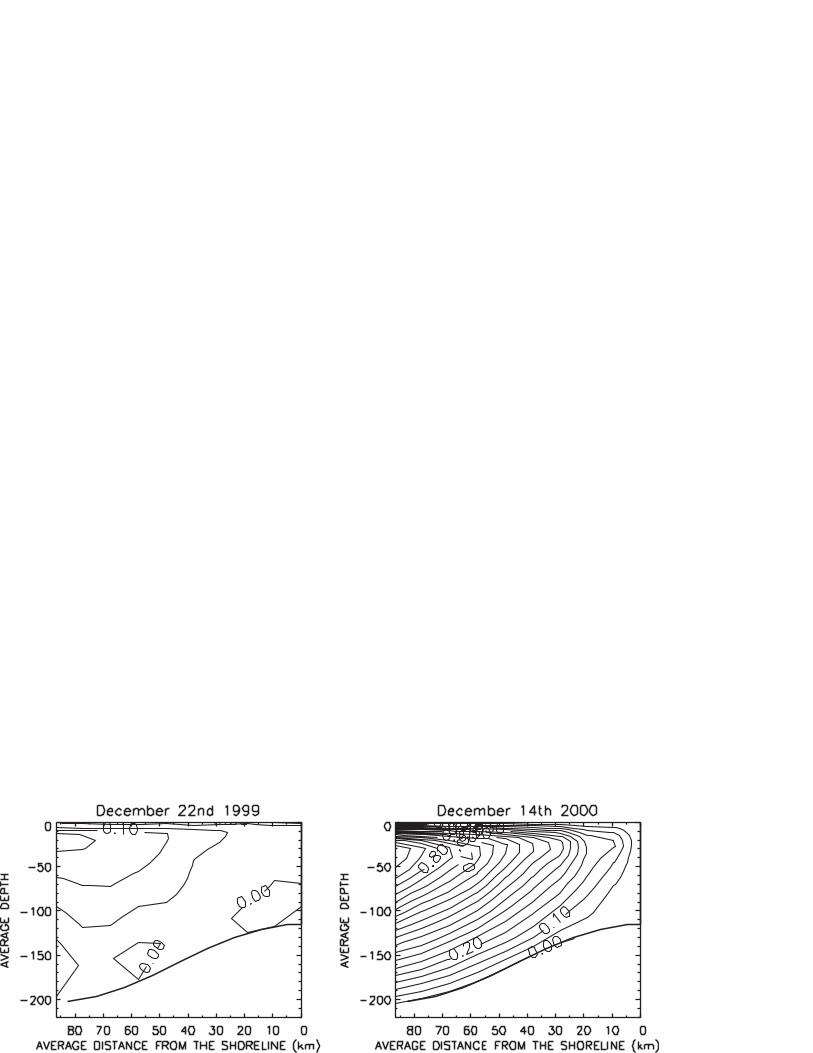
overturning almost vanishes in December 1999 (< 0.2 Sv for two consecutive weeks), letting the

surface summer heat flux warm up freely the shelf waters (Figure 16a). Conversely, in December

2000, a surge in the wind stress causes a doubling of the overturning (1 Sv for a few days, Figure

16b). This surge is responsible for a concurrent, colder than usual, signature in SST with an

upwelling circulation that penetrates over the shelf all the way to the shoreline. In the southern

Benguela, our result constitutes a model-based validation of an upwelling index often used by

fishery oceanographers [Bakun, 1973]. Despite a slight difference in the magnitude, the alongshore

wind stress appears as a reasonable qualitative substitute for the overturning circulation and

subsequent input of nutrient rich sub-surface waters on the shelf. It is likely that such a good match

between wind forcing and overturning circulation is not always the case. In areas like, for example,

the Canary Current system, where upwelling sometimes moves from the nearshore domain to the

17

shelf break [Barton et al., 1977], or the Gulf of Guinea where remotely forced coastal trapped

waves contribute to upwelling [Picaut, 1983], wind-based upwelling indices are likely unable to

condense the full underlying complex dynamics. By providing an estimate of overturning amplitude

model-based indices can be very helpful in these regions.

c) Upwelling spatial extension : Torque calculation

The spatial extent of the region affected by upwelling variability is worth being investigated.

On the edge of a domain bounded northward and southward by the yellow lines, A and B, (Figure 1

at about 27.5°S and 33°S) and on the open ocean side by any given isobath h varied from 50 m over

the shelf to 2500 m, the intensity of the upwelling circulation can be diagnosed at any time t with

the following torque calculation :

€

M(h,t) = −k s,z( )UT s,z,t( )dz dsz= bottom

surface∫∫ (6)

where z denotes depth, UT is the cross-edge velocity (counted negative when directed toward the

interior domain), s is a curvilinear coordinate following the path of isobath h and of imposed

northern and southern limits, and k(z) is the vertical mapping of depth over model terrain-following

levels (from 0 at the surface to 20 at the ocean bottom). As the model three-dimensional velocity

field is non-divergent and as there is no source or sink of mass, we have :

€

UT s,z,t( )dz dsz= bottom

surface∫∫ ≡ 0 (7)

The calculation of M does not depend on any reference value for k. For a given velocity profile, M

intensity is maximum when the inflow (negative values of UT) and the outflow (positive values of

UT) are concentrated in the bottom and uppermost model layers, respectively. On the contrary,

values close to zero denote a regime with no substantial contrast in the vertical structure of the

circulation, before and after passage in the inshore domain. Equivalent results could be obtained

with a weighting factor referring directly to depth rather than to model levels, but would lead to

more an inequity between surface and deep currents. Equation (7) is consistent with the essence of

18

terrain following levels that allow an accurate representation of layered flows over topography. It

efficiently filters incoming and outgoing eddy structures propagating along isopycnals and more

acceptably depicted by sigma levels than by geopotential levels.

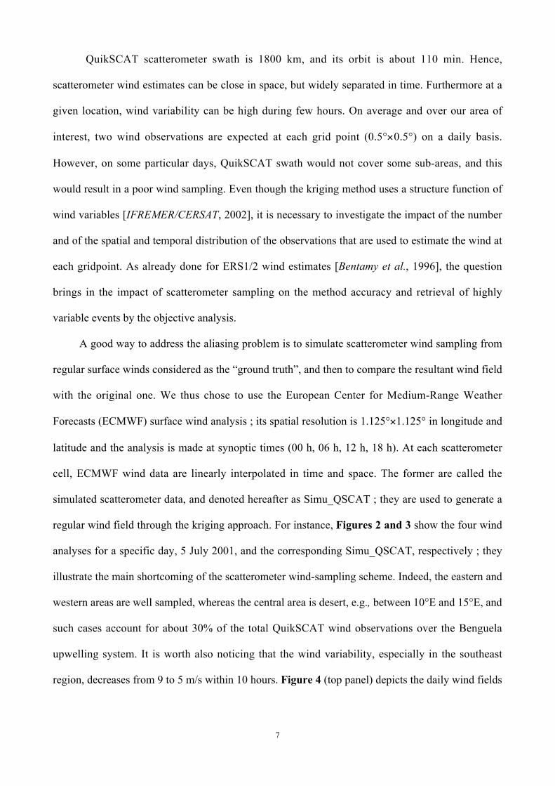
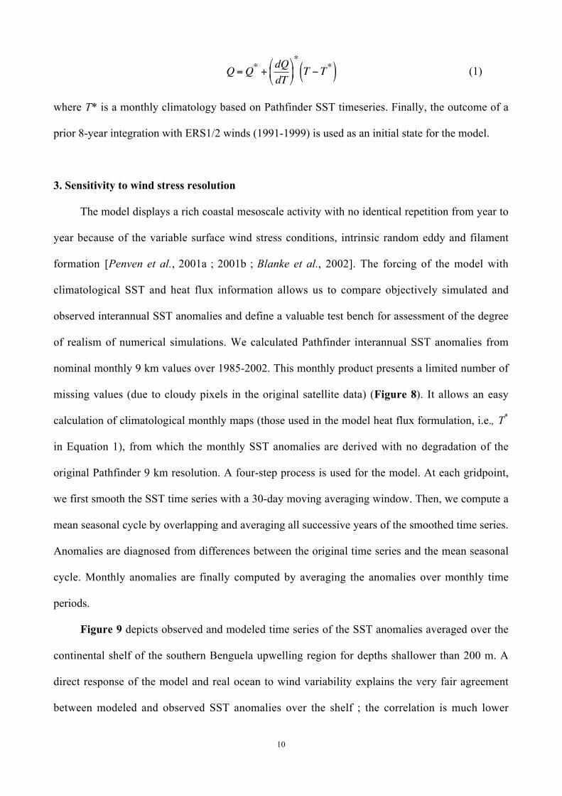
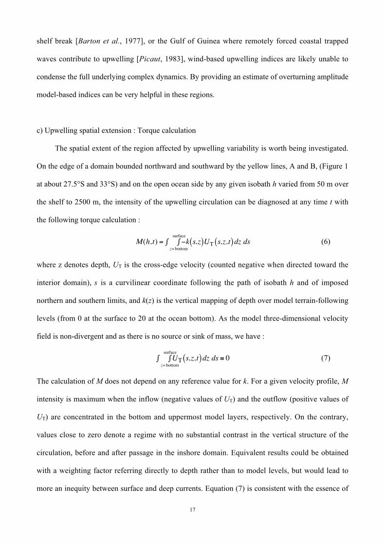
For values of h in the range 150-200 m, Figure 17 shows that M(h, t) matches very well the

time evolution of the ψ maximum : indeed, the correlation coefficient in time of both quantities is

maximum (0.924) for h = 180 m and exceeds 0.9 over the range 100-400 m. Therefore, our torque

calculation is a relevant upwelling index, which maps very well the amplitude of the overturning

above the shelf and can be used as an extension of this latter to evaluate the sensitivity of the open

ocean to upwelling processes. As the domain under study encompasses a larger offshore area, the

variability of the overturning circulation expressed by M is progressively out of phase with the

signal on the shelf edge, where the correlation with the alongshore wind stress is the greatest one

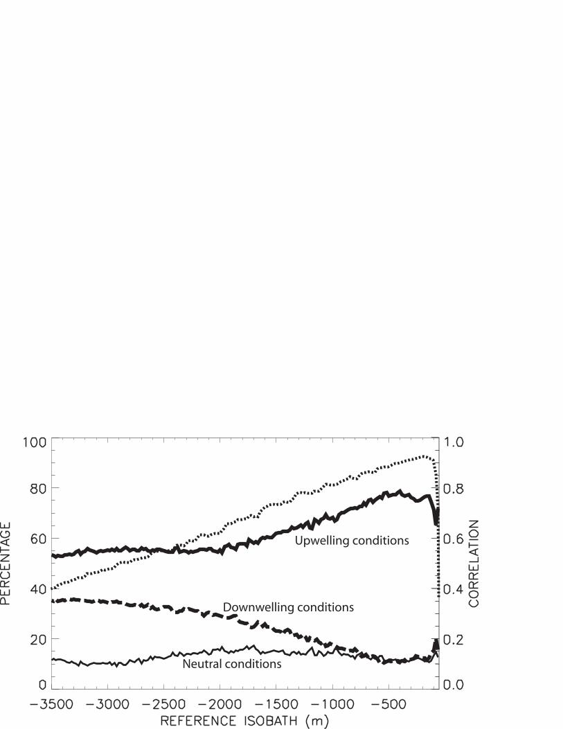
(data not shown). For each reference isobath, conditions are defined as genuine upwelling (or

downwelling) ones when positive (or negative) values of M exceeds a fifth of the standard deviation

of the time series ; other phases can be referred to neutral conditions (Figure 17). Note that

equivalent calculations can be done for ψmax, and lead to 79.5%, 18%, and 2.5% of upwelling,

downwelling and neutral conditions, respectively. The percentage of upwelling conditions

asymptotes a constant value for ocean depths greater than 2000 m (at roughly 250 km from the

coastline), whereas neutral conditions always remain within 10 and 17%. As expected, the coastal

circulation, which is directly driven by the wind stress over the shelf, shows propensity to

upwelling because the alongshore component of the wind is directed preferentially toward the

equator. Even though the wind stress curl can contribute to an offshore extent of upwelling, the

decrease of upwelling signal over the continental slope suggests that the ocean dynamical response

to changes in the surface wind forcing is partly masked by other processes offshore (e.g., mesoscale

eddies or filaments, upwelling plumes in the lee of Cape Peninsula and Cape Columbine) [Blanke et

al., 2002].

19

5. Large-scale embedding

The sensitivity of the shelf circulation to alongshore wind stress variability must not be

separated from the study of the embedment of the coastal flow in a broader regional dynamics. The

western coast of South Africa, and more specially St Helena Bay, is a major retention area for

larvae and young fish recruits ; on the other hand, spawning is mostly concentrated southeast of the

tip of South Africa, in the vicinity of the Agulhas Bank. Whatever the season, the Agulhas Current

and the shedding of retroflection eddies maintain a permanent connection between both areas

[Lutjeharms, 1996]. A technique previously proposed in Blanke and Raynaud [1997] and Blanke et

al. [1999] consists in sketching synthetic pictures of the large-scale circulation connected to the

upwelling with contours of a two-dimensional Lagrangian streamfunction to project the three-

dimensional pathways of selected water masses on a horizontal plane.

In order to derive a picture of the large-scale connections liable to serve as a basis for specific

case studies, let us focus on a pie-shaped region surrounding the upwelling region and extending

210-270 km offshore from the tip of Cape Peninsula to 27°S ; at first, we investigate the water

masses exchanged between the southeastern edge and the other ocean boundaries of this area with a

10-day velocity climatology derived from the full 1999-2003 integration (Figure 18). Calculations

are made separately for the flow exiting from and for the one coming in through the southeastern

edge. One should be aware that the resulting contours are not those of the barotropic streamfunction

given by the vertical integration of the full velocity field since the Lagrangian analysis allows one

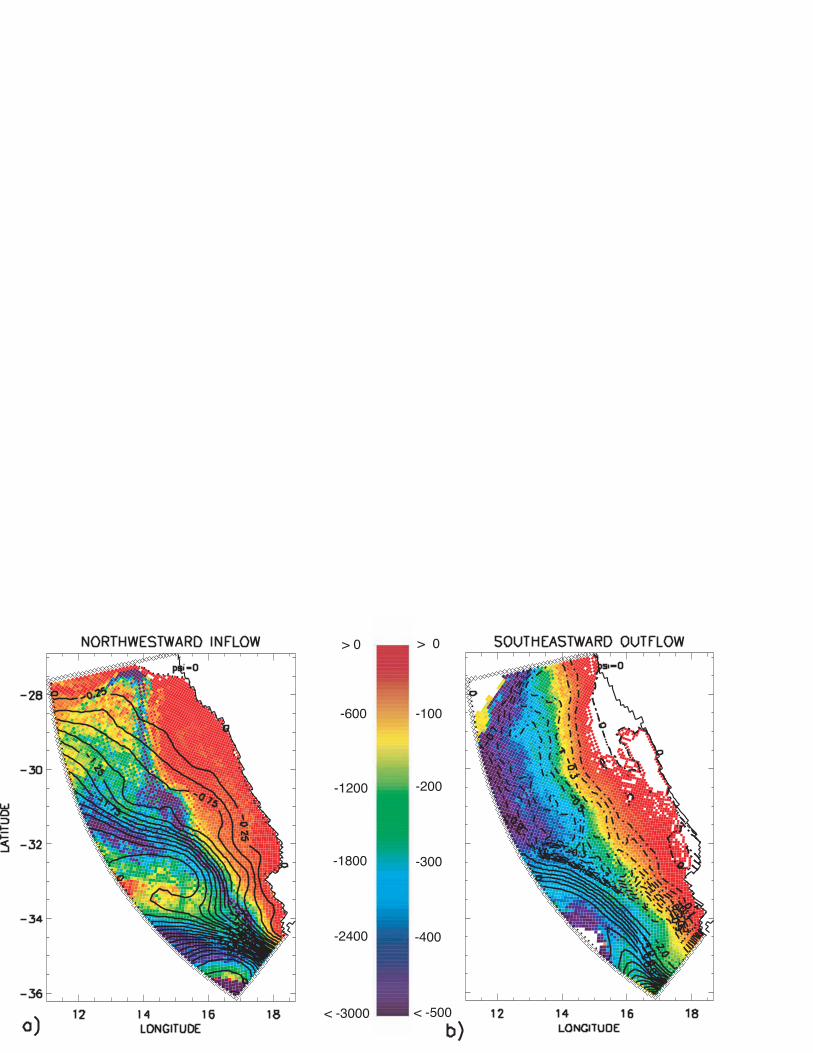
to focus on specific water masses or components of the total flow. Figure 18a shows that the

outflow is dominated by the southeastward export of Atlantic origin deep water on its way to the

Indian Ocean in good agreement with inverse modeling results by Arhan et al. [2003] ; it also

highlights the southward transmission of water against the continental slope in the form of distinct

veins. The upper vein lies within 300-500 m in depth and reminds observations of the Benguela

shelf edge poleward undercurrent by Shannon and Nelson [1996] ; a second vein (1500-3000 m) is

20

in agreement with the general description by Nelson [1989] of the deep poleward motion toward the

Cape Basin. The inflow (Figure 18b) consists of 7.0 Sv of surface water transferred northeastward

within the Benguela Current from the Agulhas Current retroflection and the South Atlantic Current

contribution [Hardman-Mountford et al., 2003]. One should note that a part of this transfer,

calculated here with climatological flow conditions, reaches the continental shelf and likely

interferes with the coastal upwelling.

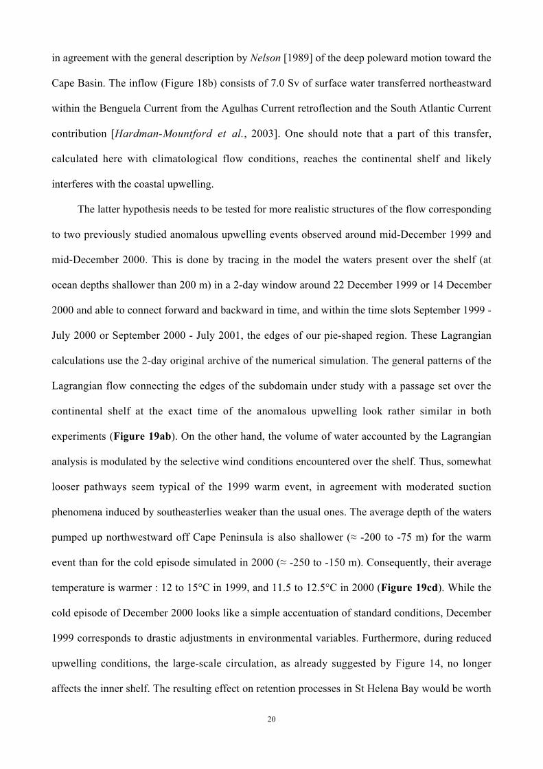
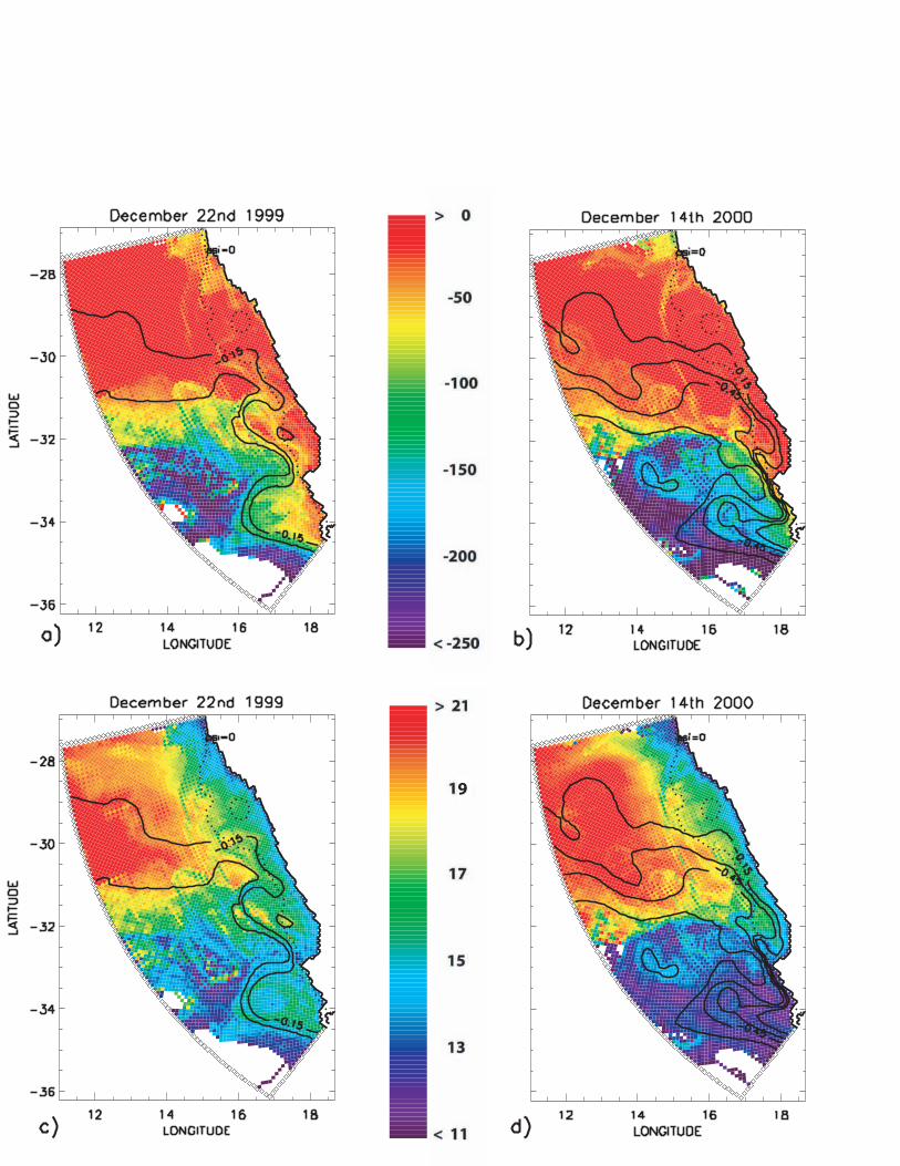
The latter hypothesis needs to be tested for more realistic structures of the flow corresponding

to two previously studied anomalous upwelling events observed around mid-December 1999 and

mid-December 2000. This is done by tracing in the model the waters present over the shelf (at

ocean depths shallower than 200 m) in a 2-day window around 22 December 1999 or 14 December

2000 and able to connect forward and backward in time, and within the time slots September 1999 -

July 2000 or September 2000 - July 2001, the edges of our pie-shaped region. These Lagrangian

calculations use the 2-day original archive of the numerical simulation. The general patterns of the

Lagrangian flow connecting the edges of the subdomain under study with a passage set over the

continental shelf at the exact time of the anomalous upwelling look rather similar in both

experiments (Figure 19ab). On the other hand, the volume of water accounted by the Lagrangian

analysis is modulated by the selective wind conditions encountered over the shelf. Thus, somewhat

looser pathways seem typical of the 1999 warm event, in agreement with moderated suction

phenomena induced by southeasterlies weaker than the usual ones. The average depth of the waters

pumped up northwestward off Cape Peninsula is also shallower (≈ -200 to -75 m) for the warm

event than for the cold episode simulated in 2000 (≈ -250 to -150 m). Consequently, their average

temperature is warmer : 12 to 15°C in 1999, and 11.5 to 12.5°C in 2000 (Figure 19cd). While the

cold episode of December 2000 looks like a simple accentuation of standard conditions, December

1999 corresponds to drastic adjustments in environmental variables. Furthermore, during reduced

upwelling conditions, the large-scale circulation, as already suggested by Figure 14, no longer

affects the inner shelf. The resulting effect on retention processes in St Helena Bay would be worth

21

being investigated because of the likely high sensitivity of biology to intensity, depth and

temperature of the advective mass inflow. This analysis provides also some insights into the

processes that have contributed to the exceptionally high anchovy recruitment that followed the

collapse of upwelling in December 1999 [Roy et al., 2001]. Figure 19 suggests that, despite the

collapse of the coastal upwelling, the pathway along the Cape Peninsula between the spawning and

nursery grounds, though being reduced, was still active in December 1999. Being transported in

warmer surface water, eggs and larvae could have found better conditions for their development and

have reached the West Coast upwelling region at a more mature stage. Reduced offshore loss

resulting from the upwelling collapse could also have had a positive impact on the success of

transport.

6. Conclusion

A correct sampling in time, at a daily scale, of the atmospheric events responsible for coastal

upwelling processes is essential to ensure a relevant representation of SST anomalies over the

southern Benguela shelf. This result was obtained with a regional model that used no data

assimilation, except for the prescription of purely climatological conditions at the surface and open

boundaries. It is very encouraging for the development of improved atmospheric fluxes for regional

and coastal ocean modeling. This study states that describing, understanding and modeling the

variability of a regional upwelling require accurate information on surface wind forcing.

Unfortunately, the QuikSCAT resolution samples poorly the wind stress curl due to the decrease of

the alongshore component near the coast, even though this effect is known to influence the system

[Fennel, 1999]. Therefore, our aim is to investigate further the enhancement of the time and space

resolution of the remotely sensed wind stress parameters. We plan to perform wind stress

estimation, at local scales, by merging satellite surface observations, including scatterometers

(ERS1/2 and QuikSCAT), radiometers (SSM/I : Special Sensor Microwave/Imager), and altimeters.

Then, the high frequencies already present in the QuikSCAT forcing are likely to generate coastally

22

trapped waves (CTWs) in the simulation. Such waves propagate southward against the Benguela

Current. Unfortunately in this study, the time resolution (2-day averages) of the model output made

difficult their correct sampling as well as the evaluation of their exact contribution to the flow over

the continental shelf. As CTWs are able to modify some characteristics of the upwelling circulation

(amplitude of sea level changes, rectification of the magnitude of the alongshore surface current),

next investigations will need to differentiate the impact of CTWs from the direct effect of the

surface wind stress.

We defined two model indices from dynamical quantities to document nearshore upwelling

intensity and upwelling spatial extension, and validated them with respect to more classical wind-

derived measurements. One should be well aware of the true spatial heterogeneity of the upwelling,

even though the development of synthetic indices provides a quantitative basis for comparison with

offshore upwelling scales given by biological processes such as those described by Carr [2002] and

Carr and Kearns [2003]. Equivalent time scales appear in both indices, but our study shows that the

dynamical signature of the upwelling is rapidly diluted offshore. Unlike western boundary

upwelling systems, the southern Benguela region is embedded in a larger scale circulation due to

the westward leaking of structures over the shelf permitted by the variations of the Coriolis force

with latitude [Kundu and McCreary, 1985 ; Marchesiello et al., 2003]. Local wind variability only

modulates the patterns of the regional connections. For two major anomalous events, the

development of synthetic circulation schemes from the Lagrangian analysis of the model velocity

and tracer fields enabled us to diagnose and accurately display the large-scale connections

established during two specific warm and cold events in the southern Benguela system. From the

importance granted to the interannual variability of the eastern boundaries upwelling regimes, with

respect to modulations in local atmospheric conditions or remote large-scale forcing, we wish to

develop the same kind of diagnostics for other upwelling systems. An accurate Lagrangian

documentation of the dynamical connections between large-scale circulation patterns and regional

23

upwelling circulation would, indeed, provide valuable help for a better understanding of the

changes in fish distribution caused, for instance, by modification of environmental constraints.

24

Acknowledgements

This study was funded by the Idyle-BEP-V project, The French Programme Atmosphère et

Océan à Multi-échelles, the French Programme National sur l’Environnement Côtier, the Institut de

Recherche pour le Développement (BB, BS, CR, SS), the Centre National de la Recherche

Scientifique (BB), the Université de Bretagne Occidentale (SS), and the Institut Français de

Recherche pour l’Exploitation de la Mer (AB). It is a pleasure to acknowledge comments and

suggestions by the editor and two anonymous reviewers that improved the legibility of the

manuscript. We are also glad to acknowledge fruitful discussions with Patrick Marchesiello and

Pierrick Penven. We thank Marie-Paule Friocourt for her expert assistance in correcting the

manuscript.

25

Reference list

Arhan, M., H. Mercier, and Y. H. Park (2003), On the deep water circulation of the eastern South

Atlantic Ocean. Deep-Sea Res. I, 50, 889-916.

Bakun, A. (1973), Daily and weekly upwelling indices, west coast of North America 1946-71. U.S.

Dep. Commer., NOAA Tech. Rep. NMFS SSRF-671, 103 p.

Bakun, A., and Nelson, C. S. (1991), The seasonal cycle of wind stress curl in subtropical eastern

boundary current regions. Journal of Physical Oceanography, 21, 1815–1834.

Bang, N. D. and W. R. H. Andrews (1974), Direct current measurements of a shelf-edge frontal jet

in the southern Benguela system. J. Mar. Res. 32(3), 405-417.

Barton E. D., A. Huyer, and R. L. Smith (1977), Temporal variation observed in the hydrographic

regime near Cabo Corbeiro in the northwest African upwelling region, February to April

1974. Deep-Sea Research, 24,7-23.

Bentamy, A., Y. Quilfen, F. Gohin, N. Grima, M. Lenaour, and J. Servain (1996), Determination

and validation of average field from ERS-1 scatterometer measurements. Global Atmos.

Ocean Sys., 4, 1-29.

Bentamy A., Y. Quilfen, and P. Flament (2002), Scatterometer wind fields : A new release over the

decade 1991 – 2001. Can. J. Remote Sensing, 28, 431-449.

Biastoch, A., and W. Krauß (1999), The role of mesoscale eddies in the source regions of the

Agulhas Current. J. Phys. Oceanogr., 29, 2303-2317.

Blanke, B., and S. Raynaud (1997), Kinematics of the Pacific Equatorial Undercurrent : An

Eulerian and Lagrangian approach from GCM results. J. Phys. Oceanogr., 27, 1038-1053.

Blanke, B., M. Arhan, G. Madec, and S. Roche (1999), Warm water paths in the equatorial Atlantic

as diagnosed with a general circulation model. J. Phys. Oceanogr., 29, 2753-2768.

Blanke, B., C. Roy, P. Penven, S. Speich, J. McWilliams, and G. Nelson (2002), Linking wind and

upwelling interannual variability in a regional model of the southern Benguela. Geophys. Res.

Lett., 29, 2188, doi :10.1029/2002GL015718.

26

Brundrit, G. B., B. A. de Cuevas, and A. M. Shipley (1987), Long-term sea-level variability in the

eastern south Atlantic and comparison with that eastern Pacific, S. Afr. J. mar. Sci., 5, 73-78.

Carr, M.-E. (2002), Estimation of potential productivity in Eastern Boundary Currents using remote

sensing. Deep-Sea Research II, 49, 59–80.

Carr, M.-E., and E. J. Kearns (2003), Production regimes in four eastern boundary current regions :

a climatological and satellite comparison. Deep Sea Research II, 50, 3199-3222.

Chin, T. M., R. F. Milliff, and W. G. Large (1998), Basin-scale, high-wavenumber sea surface wind

fields from a multiresolution analysis of scatterometer data. J. Atmos. Ocean. Tech., 15, 741-

763.

Cole, J, and C. Villacastin (2000), Sea surface temperature variability in the northern Benguela

upwelling system, and implications for fisheries research, Int. J. Remote Sens., 21, 1597-1617

Da Silva, A. M., C. C. Young, and S. Levitus, (1994) Atlas of surface marine data 1994, volume 1 :

algorithms and procedures, NOAA Atlas NESDIS 6, 74 p.

Dettinger, M. D., M. Ghil, C. M. Strong, W. Weibel, and P. Yiou (1995), Software expedites

singular-spectrum analysis of noisy time series. Eos, Trans. American Geophysical Union,

76(2), p. 12, 14, 21.

Fennel, W. (1999), Theory of the Benguela upwelling system. J. Phys. Oceanogr., 29, 177-190.

Flather, R. (1976), A tidal model of the north-west European continental shelf. Mem. Soc. R. Sci.

Liege, 10, 141-164.

Fréon, P. (2000), The IDYLE project in the Benguela : interactions and spatial dynamics of

renewable resources in upwelling systems. GLOBEC International newsletter, 6.1, p. 12.

Gordon, A. L. (1986), Interocean exchange of thermocline water. J. Geophys. Res., 91, 5037-5046.

Gordon, A. L., Bosley, K. T., and F. Aikman (1995), Tropical Atlantic water within the Benguela

upwelling system at 27°S. Deep- Sea Res. 42, 1-12.

27

Haidvogel, D. B., H. Arango, K. Hestrom, A. Beckmann, P. Malanotte-Rizzoli, and A. Shchepetkin

(2000), Model evaluation experiments in the North Atlantic basin : simulations in nonlinear

terrain-following coordinates. Dyn. Atmos. Oceans, 32, 239-381.

Hardman-Mountford, N. J., A. J. Richardson, J. J. Agenbag, E. Hagen, L. Nykjaer, F. A.

Shillington, and C. Villacastin (2003), Ocean climate of the South East Atlantic observed

from satellite data and wind models. Prog. Oceanogr., 59, 181-221.

Hutchings, L., Pitcher, G. C., Probyn, T. A., and G. W. Bailey (1995), The chemical and biological

consequences of coastal upwelling. In Upwelling in the Ocean : Modern Processes and

Ancient Records. Edited by Summerhayes, C. P., Emeis, K-C., Angel, M. V., Smith, R. L.,

and B. Zeitzschel, pp. 64-81, John Wiley & Sons Ltd, New York.

IFREMER/CERSAT (2002), QuikSCAT Scatterometer Mean Wind Field Products User Manual.

C2-MUT-W-04-IF, version 1.0, IFREMER/CERSAT, Plouzané, France.

Jury, M. R. (1986), The sudden decay of upwelling off the cape peninsula, South Africa : a case

study. S. Afr. J. mar. Sci., 4, 111-118.

Kundu, P. K., and J. P. McCreary (1985), Western boundary circulation driven by an alongshore

wind : with application to the Somali Current system. J. Mar. Res., 43, 493-516.

Lutjeharms, J. R. E. (1996), The exchange of water between the South Indian and the South

Atlantic, In The South Atlantic : Present and Past Circulation, edited by G. Wefer, W. H.

Berger, G. Siedler and D. Webb, pp. 125-162, Springer-Verlag, Berlin.

Marchesiello, P., J. C. McWilliams, and A. Shchepetkin (2001), Open boundary conditions for

long-term integration of regional oceanic models. Ocean Modelling, 3, 1-20.

Marchesiello, P., J. C. McWilliams, and A. Shchepetkin (2003), Equilibrium structure and

dynamics of the California Current system. J. Phys. Oceanog., 33, 753-783.

Nelson, G., and L. Hutchings (1983), The Benguela upwelling system. Prog. Oceanogr., 12, 333-

356.

28

Nelson, G. (1989), Poleward motion in the Benguela area. In Coastal and Estuarine Studies, 34,

Poleward flows along eastern ocean boundaries, edited by S. J. Neshyba, C. N. K. Mooers, R.

L. Smith, and R. T. Barber, pp. 110-130, Springer, New York.

Nelson, G. (1992), Equatorward wind and atmospheric pressure spectra as metrics for primary

productivity in the Benguela system. S. Afr. J. mar. Sci., 12, 19-28.

Payne, A. I. L., K. H. Brink, K. H. Mann, and R. Hilborn (Eds.) (1992), Benguela trophic

functioning. S. Afr. J. mar. Sci., 12, 1108 pp.

Penven, P., C. Roy, G. B. Brundrit, A. Colin de Verdière, P. Fréon, A. S. Johnson, J. R. E.

Lutjeharms, and F. A. Shillington (2001), A regional hydrodynamic model of the Southern

Benguela upwelling. S. Afr. J. Sci., 9, 472-475.

Penven, P, J. R. E. Lutjeharms, P. Marchesiello, C. Roy, and S. J. Weeks (2001), Generation of

cyclonic eddies by the Agulhas Current in the lee of the Agulhas Bank. Geophys. Res. Lett.,

27, 1055-1058.

Picaut, J. (1983), Propagation of the seasonal upwelling in the eastern equatorial Atlantic. J. Phys.

Oceanogr., 13, 18-37.

Pillar, S. C., C. Moloney, A. I. L. Payne, and F. A. Shillington (Eds.) (1998), Benguela dynamics.

S. Afr. J. mar. Sci. 19, 512 pp.

Rintoul, S. R. (1991), South Atlantic interbasin exchange. J. Geophys. Res., 96, 2675-2692.

Roy, C., S. J. Weeks, M. Rouault, G. Nelson, R. Barlow, and C. D. van der Lingen (2001), Extreme

oceanographic events recorded in the southern Benguela during the 1999-2000 summer

season. S. Afr. J. Sci., 97, 465-471.

Schumann and Brink (1990), Coastal-trapped waves off the coast of South Africa : generation,

propagation and current structures, J. Phys. Oceanogr., 20, 1206-1218.

Shannon, L. V. (1985), The Benguela Ecosystem, Part I. Evolution of the Benguela, physical

features and processes. Oceanography and Marine Biology : An Annual Review, 23, 105–182.

29

Shannon, L. V, A. J. Boyd, G. B. Brundrit, and J. Taunton-Clark (1986), On the existence of an El-

Niño type phenomenon in the Benguela system. J. Mar. Res., 44(3), 495-520.

Shannon, L. V., and G. Nelson (1996), The Benguela : Large scale features and processes and

system variability, In The South Atlantic past and present circulation, edited by G. Wefer, W.

H. Berger, G. Siedler, and D. J. Webb, pp. 163-210, Springer Verlag, Berlin, Heidelberg.

Shannon, L. V., and S. C. Pillar (1986), The Benguela ecosystem. 3. Plankton. In Oceanography

and Marine Biology. An Annual Review 24, edited by M. Barnes, pp. 65-170, Aberdeen,

University Press.

Shillington, F. A. (1998), The Benguela upwelling system off southwestern Africa, In The Sea, Vol.

11, The global coastal ocean, regional studies and syntheses, edited by A. R. Robinson and

K. H. Brink, pp. 583-604, Wiley, New-York.

30

Table and Figure captions

Table 1. Statistical parameters characterizing the difference between ECMWF and simulated

QuikSCAT wind field data.

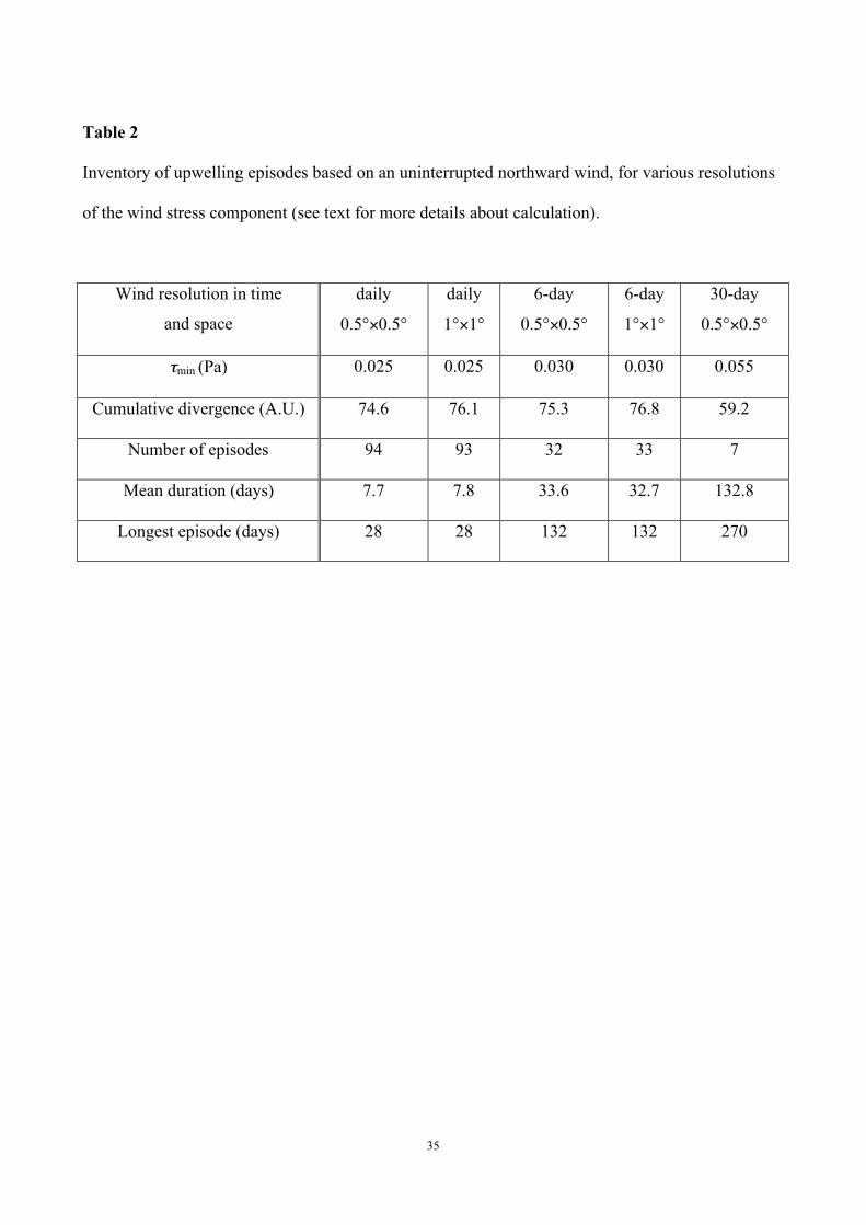
Table 2. Inventory of upwelling episodes based on an uninterrupted northward wind and for

various resolutions of the wind stress component (see text for more details about calculation).

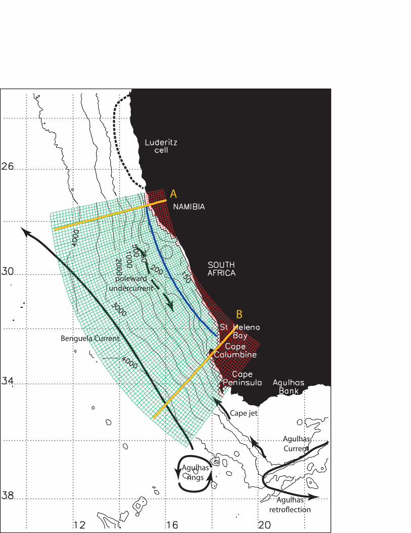
Figure 1. Model horizontal grid, horizontal system of coordinates and ocean bathymetry in the

neighborhood of the Benguela upwelling. The colored area is the focus of our study. The shelf

domain bounded by the blue line is used in the definition of an overturning streamfunction (see

section 4b). Yellow lines A and B delimit the meridional extension of the area encompassed by a

torque calculation (see section 4c).

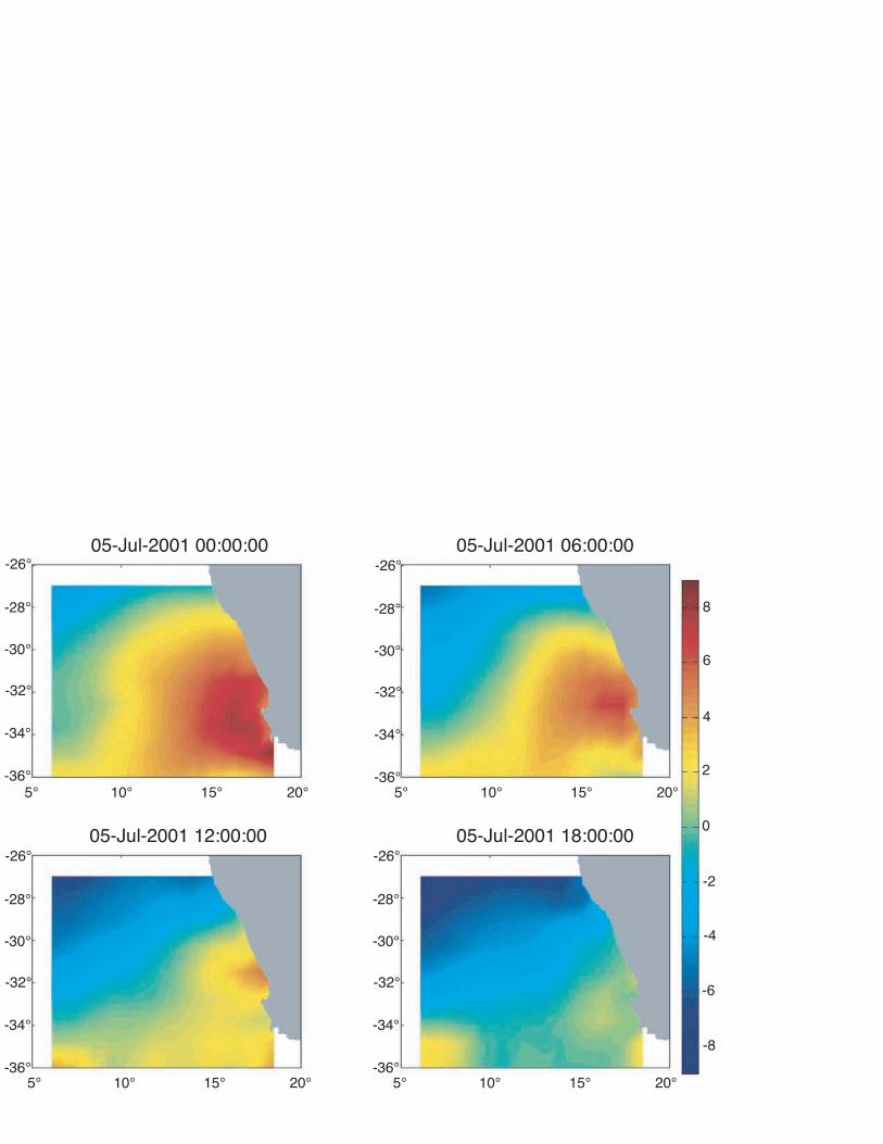
Figure 2. ECMWF surface zonal wind analyses of 5 July 2001 (in m/s).

Figure 3. ECMWF surface zonal wind component interpolated over QuikSCAT swaths during July

5th, 2001. The color scale gives the wind intensity in m/s.

Figure 4. Daily averaged zonal wind field calculated from ECMWF wind analysis interpolated over

scatterometer swaths (top) and from the four ECMWF wind analyses of 5 July 2001 (bottom). The

color scale shows the wind intensity in m/s.

Figure 5. Time-lagged correlation between anemometer-derived pseudo-stress and QuikSCAT-

derived wind stress over the period from 1 September 1999 to 14 January 2001 at the nearest

collocation gridpoint, for the meridional (top) and zonal (bottom) components.

31

Figure 6. (a) Daily averaged Cape Columbine anemometer meridional pseudo-stress (in m2/s2). (b)

Daily QuikSCAT-derived meridional pseudo-stress (in Pa).

Figure 7. Power spectra (arbitrary units) of the anemometer-derived meridional pseudo-stress and

QuikSCAT-derived meridional wind stress over their overlapping period.

Figure 8. Percentage of missing values in monthly 9-km Pathfinder SST data over the period 1999-

2003 in the ocean area surrounding southwest Africa.

Figure 9. Monthly time series of shelf SST anomalies for the model (dotted line, left-hand axis) and

Pathfinder observations (solid line, right-hand axis). Warm or cold events with anomalies exceeding

1.5°C in observations are highlighted.

Figure 10. SST anomaly maps for December 1999 (a and b) and December 2000 (c and d). The

contour interval is 0.5 and 0.3°C for the observations (a and c) and the model (b and d),

respectively. Note that the color scales have been adjusted to make model and observed anomalies

similar.

Figure 11. Correlation map of interannual Pathfinder and simulated monthly SST anomalies. The

model is forced by the following QuikSCAT-derived wind stress products : (a) daily 0.5°×0.5°

(nominal resolution). (b) 6-day 0.5°×0.5°. (c) 1-day 1°×1°. (d) monthly 0.5°×0.5°. Isobath 200 m is

dotted. Contour interval (0.1) and color scale are the same in all panels.

32

Figure 12. Same as Figure 11, but for the ERS wind stress with its nominal weekly 1°×1°

resolution. The contour interval is 0.1.

Figure 13. Average of four successive December-January periods for the QuikSCAT wind. (a)

wind stress curl (10-7 Pa m-1) with dots over regions of cyclonic curl. (b) wind stress intensity (Pa)

with a 0.01 Pa contour interval.

Figure 14. Time mean cross-shore velocity time series in the outer shelf region. Negative dotted

values denote coastward movements. The contour interval is 2×10-2 m/s. Shaded areas denote a

linear time correlation with the alongshore wind component greater than 0.4.

Figure 15. Time series of two upwelling indices over November 1999 - February 2000 and

November 2000 - February 200. Alongshore wind stress component (solid line and left axis).

Maximum value of the shelf overturning ψ(x, z) (dotted line and right axis).

Figure 16. Shelf overturning streamfunction. (a) ψ(x, z) on December 22nd 1999. (b) ψ(x, z) on 14

December 2000. The contour interval is 0.05 Sv.

Figure 17. Fraction of upwelling, downwelling and neutral conditions diagnosed from the analysis

of M(h, t). The linear correlation coefficient between M(h, t) and the maximum value of the shelf

overturning streamfunction (ψmax) is superimposed as a dotted line (right-hand axis).

Figure 18. Mass exchanges achieved between the southeastern and the other edges of a pie-shaped

region surrounding the upwelling region. (a) southeastward outflow, with a mixed 1 Sv (solid) -

0.1 Sv (dotted) contour interval. (b) northwestward inflow, with a 0.25 Sv contour interval. Color

33

shows the average depth (in meters) of the advective flow. Note the difference in depth scale

between both panels.

Figure 19. Upwelling circulation schemes restricted to water masses reaching the shelf at selected

moments. (a and c) around 22 December 1999. (b and d) and 14 December 2000. Color shows the

average depth (a and b) or the average temperature (c and d) of the advective flow. The contour

interval is 0.15 Sv.

34

Table 1

Statistical parameters characterizing the difference between ECMWF and simulated QuikSCAT

wind field data.

Wind speed (m/s) Wind direction (°)

Number of data Mean Standard deviation Mean Standard deviation

July 6782 -0.29 1.61 -5 17

December 6816 0.02 0.85 1 13

35

Table 2

Inventory of upwelling episodes based on an uninterrupted northward wind, for various resolutions

of the wind stress component (see text for more details about calculation).

Wind resolution in time

and space

daily

0.5°×0.5°

daily

1°×1°

6-day

0.5°×0.5°

6-day

1°×1°

30-day

0.5°×0.5°

τmin (Pa) 0.025 0.025 0.030 0.030 0.055

Cumulative divergence (A.U.) 74.6 76.1 75.3 76.8 59.2

Number of episodes 94 93 32 33 7

Mean duration (days) 7.7 7.8 33.6 32.7 132.8

Longest episode (days) 28 28 132 132 270

Agulhas

Current

Agulhas

retroflection

Agulhas

rings

Benguela Current

Cape jet

poleward

undercurrent

A

B

05-Jul-2001 00:00:00

05-Jul-2001 18:00:0005-Jul-2001 12:00:00

05-Jul-2001 06:00:00

5° 10° 15° 20°

5° 10° 15° 20° 5° 10° 15° 20°

5° 10° 15° 20°

-26°

-28°

-30°

-32°

-34°

-36°

-26°

-28°

-30°

-32°

-34°

-36°

-26°

-28°

-30°

-32°

-34°

-36°

-26°

-28°

-30°

-32°

-34°

-36°

8

6

4

2

0

-2

-4

-6

-8

05-Jul-2001 04:25:21

05-Jul-2001 16:12:3205-Jul-2001 14:31:30

05-Jul-2001 06:06:22

5° 10° 15° 20°

5° 10° 15° 20° 5° 10° 15° 20°

5° 10° 15° 20°

-26°

-28°

-30°

-32°

-34°

-36°

-26°

-28°

-30°

-32°

-34°

-36°

-26°

-28°

-30°

-32°

-34°

-36°

-26°

-28°

-30°

-32°

-34°

-36°

8

6

4

2

0

-2

-4

-6

-8

11

10

9

8

7

6

5

-27°

-28°

-29°

-30°

-31°

-32°

-33°

-27°

-28°

-29°

-30°

-31°

-32°

-33°

10° 12° 14° 16° 18° 20°

10° 12° 14° 16° 18° 20°

Upwelling conditions

Downwelling conditions

Neutral conditions

> 0

-100

-200

-300

-400

< -500

> 0

-600

-1200

-1800

-2400

< -3000

9