Modeling the spatio-temporal evolution of fracture networks and fluid-rock interactions in GPU: Applications to lithospheric geodynamics Dissertation zur Erlangung des Doktorgrades (Dr. rer. nat.) der Mathematisch-Naturwissenschaftlichen Fakult¨ at der Rheinischen Friedrich-Wilhelms-Universit¨ at Bonn vorgelegt von Boris Galvan aus Panama Stadt, Republik Panama Bonn 2012

Welcome message from author
This document is posted to help you gain knowledge. Please leave a comment to let me know what you think about it! Share it to your friends and learn new things together.
Transcript
Modeling the spatio-temporal
evolution of fracture networks and
fluid-rock interactions in GPU:
Applications to lithospheric
geodynamics
Dissertation
zur
Erlangung des Doktorgrades (Dr. rer. nat.)
der
Mathematisch-Naturwissenschaftlichen Fakultat
der
Rheinischen Friedrich-Wilhelms-Universitat Bonn
vorgelegt von
Boris Galvan
aus
Panama Stadt, Republik Panama
Bonn 2012
Angefertigt mit Genehmigung der Mathematisch-Naturwissenschaftlichen Fakultatder Rheinischen Friedrich-Wilhelms-Universitat Bonnam Steinmann-Institut fur Geologie, Mineralogie und Palaontologie
1. Referent: Prof. Dr. Stephen A. Miller2. Referent: Prof. Dr. Andreas Kemna
Tag der Promotion:Erscheinungsjahr: 2013
Diese Dissertation ist auf dem Hochschulschriftenserver der ULB Bonnhttp://hss.ulb.uni-bonn.de/diss online elektronisch publiziert.

iii

iv
Contents
Abstract 1
I INTRODUCTION 5
Introduction 7
1 Introduction 71.1 Theoretical Background . . . . . . . . . . . . . . . . . . . . . . . . . 11
1.1.1 Poro-elasto-plastic Model . . . . . . . . . . . . . . . . . . . . . 111.2 Graphical Processing Units (GPUs) in Scientific Numerical Modeling 16
1.2.1 GPU implementation of Poro-elasto-plastic Media . . . . . . . 161.2.2 GPU Architecture and Programing . . . . . . . . . . . . . . . 19
1.3 Summary of the Scientific Articles . . . . . . . . . . . . . . . . . . . . 211.3.1 A full GPU simulation of evolving fracture networks in a het-
erogeneous poro-elasto-plastic medium with effective-stress-dependent permeability . . . . . . . . . . . . . . . . . . . . . . 21
1.3.2 GPU numerical reproduction of hydrofracture experiments inPoro-elasto-plastic material . . . . . . . . . . . . . . . . . . . 21
1.3.3 Simulation of fluid induced seismicity accelerated in GPU. Ap-plication to Enhance Geothermal Systems . . . . . . . . . . . 21
1.3.4 A poro-elasto-plastic model to simulate earthquake-volcanointeraction dynamics in Central Chile . . . . . . . . . . . . . . 22
II PAPERS 23
Paper I 25
2 A full GPU simulation of evolving fracture networks in a heteroge-neous poro-elasto-plastic medium with effective-stress-dependentpermeability 252.1 Abstract . . . . . . . . . . . . . . . . . . . . . . . . . . . . . . . . . . 252.2 Introduction . . . . . . . . . . . . . . . . . . . . . . . . . . . . . . . . 262.3 Model equations . . . . . . . . . . . . . . . . . . . . . . . . . . . . . . 27
2.3.1 GPU implementation . . . . . . . . . . . . . . . . . . . . . . . 28
v
vi CONTENTS
2.3.1.1 GPU nonlinear diffusion implementation . . . . . . . 302.3.1.2 GPU elasto-plasticity implementation . . . . . . . . 30
2.4 Results . . . . . . . . . . . . . . . . . . . . . . . . . . . . . . . . . . . 322.4.1 Nonlinear diffusion benchmark . . . . . . . . . . . . . . . . . . 322.4.2 Elasto-plastic benchmark . . . . . . . . . . . . . . . . . . . . . 322.4.3 Poro-elasto-plastic modeling . . . . . . . . . . . . . . . . . . . 33
2.5 Conclusions . . . . . . . . . . . . . . . . . . . . . . . . . . . . . . . . 372.6 Acknowledgments . . . . . . . . . . . . . . . . . . . . . . . . . . . . . 39
Paper II 40
3 GPU numerical reproduction of hydrofracture experiments in Poro-elasto-plastic material 413.1 Abstract . . . . . . . . . . . . . . . . . . . . . . . . . . . . . . . . . . 413.2 Introduction . . . . . . . . . . . . . . . . . . . . . . . . . . . . . . . . 413.3 Theoretical Model . . . . . . . . . . . . . . . . . . . . . . . . . . . . . 433.4 GPU implementation . . . . . . . . . . . . . . . . . . . . . . . . . . . 443.5 Numerical Model of Hydrofracturing in Triaxial Experiments . . . . . 453.6 Results and Discussion . . . . . . . . . . . . . . . . . . . . . . . . . . 463.7 Conclusions . . . . . . . . . . . . . . . . . . . . . . . . . . . . . . . . 483.8 Acknowledgments . . . . . . . . . . . . . . . . . . . . . . . . . . . . . 52
Paper III 53
4 Simulation of fluid induced seismicity accelerated in GPU. Appli-cation to Enhance Geothermal Systems 534.1 Abstract . . . . . . . . . . . . . . . . . . . . . . . . . . . . . . . . . . 534.2 Introduction . . . . . . . . . . . . . . . . . . . . . . . . . . . . . . . . 534.3 Poro-elasto-plastic model . . . . . . . . . . . . . . . . . . . . . . . . . 564.4 GPU implementation . . . . . . . . . . . . . . . . . . . . . . . . . . . 574.5 Fluid injection in heterogeneous fractured rock . . . . . . . . . . . . . 584.6 Modeling the Deep Heat Mining Project in Basel . . . . . . . . . . . 604.7 Discussion and Conclusion . . . . . . . . . . . . . . . . . . . . . . . . 654.8 Acknowledgments . . . . . . . . . . . . . . . . . . . . . . . . . . . . . 65
Paper IV 66
5 A poro-elasto-plastic model to simulate earthquake-volcano inter-action dynamics in Central Chile 675.1 Abstract . . . . . . . . . . . . . . . . . . . . . . . . . . . . . . . . . . 675.2 Introduction . . . . . . . . . . . . . . . . . . . . . . . . . . . . . . . . 675.3 Geodynamic setting . . . . . . . . . . . . . . . . . . . . . . . . . . . . 695.4 Two-dimensional model . . . . . . . . . . . . . . . . . . . . . . . . . 69
5.4.1 Conceptual model . . . . . . . . . . . . . . . . . . . . . . . . . 695.4.2 Numerical model . . . . . . . . . . . . . . . . . . . . . . . . . 71
5.5 Conclusions . . . . . . . . . . . . . . . . . . . . . . . . . . . . . . . . 78
CONTENTS vii
5.6 Acknowledgments . . . . . . . . . . . . . . . . . . . . . . . . . . . . . 78
III CONCLUDING REMARKS 79
Conclusions 81
6 Concluding Remarks and Future Work 81
List of Figures 98
List of Tables and Listings 105
Acknowledgments 107

viii CONTENTS
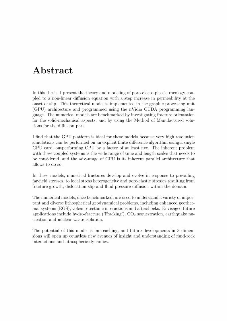
Abstract
In this thesis, I present the theory and modeling of poro-elasto-plastic rheology cou-pled to a non-linear diffusion equation with a step increase in permeability at theonset of slip. This theoretical model is implemented in the graphic processing unit(GPU) architecture and programmed using the nVidia CUDA programming lan-guage. The numerical models are benchmarked by investigating fracture orientationfor the solid-mechanical aspects, and by using the Method of Manufactured solu-tions for the diffusion part.
I find that the GPU platform is ideal for these models because very high resolutionsimulations can be performed on an explicit finite difference algorithm using a singleGPU card, outperforming CPU by a factor of at least five. The inherent problemwith these coupled systems is the wide range of time and length scales that needs tobe considered, and the advantage of GPU is its inherent parallel architecture thatallows to do so.
In these models, numerical fractures develop and evolve in response to prevailingfar-field stresses, to local stress heterogeneity and pore-elastic stresses resulting fromfracture growth, dislocation slip and fluid pressure diffusion within the domain.
The numerical models, once benchmarked, are used to understand a variety of impor-tant and diverse lithospherical geodynamical problems, including enhanced geother-mal systems (EGS), volcano-tectonic interactions and aftershocks. Envisaged futureapplications include hydro-fracture (’Fracking’), CO2 sequestration, earthquake nu-cleation and nuclear waste isolation.
The potential of this model is far-reaching, and future developments in 3 dimen-sions will open up countless new avenues of insight and understanding of fluid-rockinteractions and lithospheric dynamics.

2 ABSTRACT

Zusammenfassung
In dieser Arbeit prasentiere ich die Theorie und die Modellierung von poro- elastisch-plastischer Rheologie gekoppelt mit einer nicht-linearen Diffusionsgleichung und miteiner schrittweisen Erhohung der Permeabilitat bei dem Auftreten eines Bruches.Dieses theoretische Modell ist implementiert mit der Technologie von graphischenProzessor Einheiten (GPU) und programmiert in der nVidia CUDA Programmier-sprache.
Das numerische Modell ist benchmarked mit der Untersuchung von Orientierungenvon Bruchen fur gesteinsmechanische Aspekte und unter Verwendung der Methodeder ”Manufactured solutions” fur den diffusiven Anteil.
Ich denke, dass die GPU Plattform ideal fur diese Modelle ist, da Losungen mit sehrhoher Auflosung mit einem expliziten Finite Differenzen Algorithmus mit nur einereinzeln GPU Karte berechnet werden konnen und dabei CPU um den Faktor Funfubertreffen.
Das inharente Problem dieser gekoppelten Systeme ist die große Spannweite vonZeit- und Langenskalen, die analysiert werden mussen und der Vorteil von GPU istdie inharente parallele Struktur, die dies ermoglicht.In diesen Modellen entstehen und entwickeln sich Bruche in Antwort auf dominierendeFernfeld- Spannungen, lokale Spannungsheterogenitat, poro- elastische Spannungenresultierend aus dem Bruchwachstum, Versetzungsstufen und der Diffusion von Flu-iddruck.
Die numerischen Modelle werden, nach dem Benchmarking, verwendet um eineVielzahl von wichtigen und verschiedenen lithospharischen geodynamischen Proble-men zu verstehen, zum Beispiel Enhanced Geothermal Systems (EGS), vulkanisch-tektonische Interaktion und Nachbeben. Vorstellbare zukunftige Anwendungen bein-halten Hydro- Fracturing (’Fracking’), CO2 Sequestration, das Auslosen von Erd-beben und nukleare Endlagerung.
Das Potential dieses Modells ist weitreichend und zukunftige Entwicklungen in dreiDimensionen werden zahlreiche neue Einblicke und ein tieferes Verstandnis vonFluid- Stein Interaktionen sowie der lithospharischen Dynamik ermoglichen.
3

4 ABSTRACT

Part I
INTRODUCTION
5

Chapter 1
Introduction
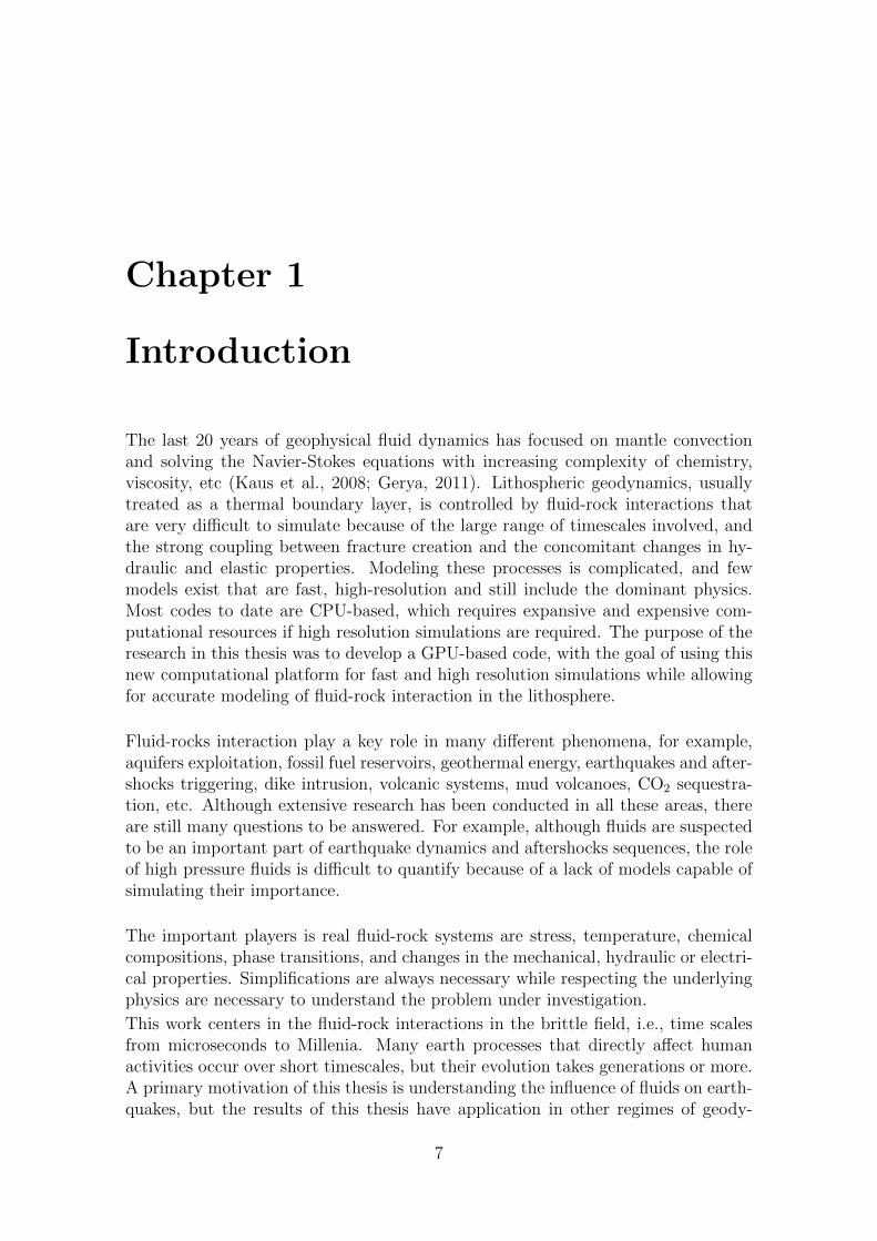
The last 20 years of geophysical fluid dynamics has focused on mantle convectionand solving the Navier-Stokes equations with increasing complexity of chemistry,viscosity, etc (Kaus et al., 2008; Gerya, 2011). Lithospheric geodynamics, usuallytreated as a thermal boundary layer, is controlled by fluid-rock interactions thatare very difficult to simulate because of the large range of timescales involved, andthe strong coupling between fracture creation and the concomitant changes in hy-draulic and elastic properties. Modeling these processes is complicated, and fewmodels exist that are fast, high-resolution and still include the dominant physics.Most codes to date are CPU-based, which requires expansive and expensive com-putational resources if high resolution simulations are required. The purpose of theresearch in this thesis was to develop a GPU-based code, with the goal of using thisnew computational platform for fast and high resolution simulations while allowingfor accurate modeling of fluid-rock interaction in the lithosphere.
Fluid-rocks interaction play a key role in many different phenomena, for example,aquifers exploitation, fossil fuel reservoirs, geothermal energy, earthquakes and after-shocks triggering, dike intrusion, volcanic systems, mud volcanoes, CO2 sequestra-tion, etc. Although extensive research has been conducted in all these areas, thereare still many questions to be answered. For example, although fluids are suspectedto be an important part of earthquake dynamics and aftershocks sequences, the roleof high pressure fluids is difficult to quantify because of a lack of models capable ofsimulating their importance.
The important players is real fluid-rock systems are stress, temperature, chemicalcompositions, phase transitions, and changes in the mechanical, hydraulic or electri-cal properties. Simplifications are always necessary while respecting the underlyingphysics are necessary to understand the problem under investigation.
This work centers in the fluid-rock interactions in the brittle field, i.e., time scalesfrom microseconds to Millenia. Many earth processes that directly affect humanactivities occur over short timescales, but their evolution takes generations or more.A primary motivation of this thesis is understanding the influence of fluids on earth-quakes, but the results of this thesis have application in other regimes of geody-
7

8 Introduction
namics, including volcanic eruptions and geothermal systems.. This work presentstudies of different problems with different scales, in time and space, from laboratorytriaxial experiments with time scales of minutes to aftershocks sequences modelingwith duration of weeks and months, to volcanic systems with timescales of centuries.
We approach these problems using continuum mechanics, in particular, the poro-mechanics formulation. The combined behavior of rock infiltrated by water wasinitially studied for engineering applications, and Karl von Terzaghi was the firstto analyze fluid saturated rocks from the point of view of poro-mechanics. Hedeveloped a one dimensional model of consolidation using a conceptual model ofwater-saturated soil grains forming an elastic porous skeleton(Terzaghi, 1923). Thisconceptualization proved to be useful for successfully predicting settlement of struc-tures for many types of soils and set the basis for poro-mechanics.
Later, Maurice A. Biot generalize the theory to three dimensions. This theorybecame what is now known as poro-elasticity (Biot, 1941). The primary two mech-anisms affecting porous media are increasing fluid pressure that causes the rock todilate, and rock compression that causes the fluid pressure to rise if the fluid cannotdrain. If the fluid pressures dissipate, the solid skeleton deforms. When part ofthe pressure exerted over the porous media is carried by the fluid, then undrainedporous media is stiffer than a drained one. The Biot formulation was the first theoryto be consistent with these observations.
If porous rock is subjected to further deformation, it yields and fractures. Thisirreversible deformation is called plasticity. Most natural rocks are porous and frac-tured. Fractures can be modeled using the porous media approach by changing thehydraulic and elastic properties in a localized way.
We model the complex mechanics of the fully couple poro-elasto-plastic media giv-ing special attention to the initiation and evolution of fracture networks as they arecreated and propagate in response to the evolving stress field.The physics involved in these processes are not amenable to analytical solutions, sonumerical methods are necessary to study realistic problems.
There are many different code available to simulate rock-fluid interactions. For ex-ample, GEOCRACK is a 2D simulator of fluid flow through fracture media thatcouples deformation, fluid flow and heat flow. UDEC is 2D simulator that couplesdeformation and fluid flow, while ROCMAS is a 3D finite element simulator of twophase flow , poroelasticity and thermoelasticity (Rutqvist and Tsang, 2003). FRAC-ture is a finite element poro-elastic, thermo-elastic simulator (Kohl et al., 1995), andGeoSys/Rockflow is a finite element 3D, multiphase flow, fracture flow, heat trans-port, chemical processes, poro-elastic, thermo-elastic and elasto-plastic simulator(Kolditz and Chen, 2005; Wang and Kolditz, 2007). MOTIF (Model Of TransportIn Fractured porous media) is a 3D finite element thermomechanical-groundwaterflow-heat flow simulator (Guvanasem and Chan, 1995), and FRANCON is finite

Introduction 9
element based 3D simulator of thermo and poroelasticity. TOUGH-FLAC a heatflow-fluid flow-mechanical simulator with capabilities for elasto-plastic deformation(Rutqvist, 2011), and is widely used in the field. Beside these codes, there is a vastnumber of ad-hoc university programs available. However all these codes, althoughthe degree of sophistication of many of them is quite advanced, lack of the necessaryresolution or speed to deal with irregular evolutionary fracture networks.
Fracture networks are the primary fluid flow channels controlling the fluid pressureprofile and which affect the overall stress state. It is clear that fracture networkscould have a very complex geometry at different scales. In processes like fluid in-duced fracturing for geothermal applications, CO2 sequestration or hydrofracturing(’fracking’), an accurate description of the network development and geometry iscrucial. A realistic description of the evolving system could help reduce cost, max-imize recovery, assess seismic hazard, and maximizes productivity and efficiency inthe reservoir exploitation or storagevity of CO2. For example, in exploitation offossil fuel reservoirs, it is necessary to simulate the behavior of the reservoirs toestimate the best points to drill the extraction and injection wells. Currently thisis done solving a flow equation in 3D and neglecting the deformation of the reser-voir, which clearly will considerably change the state of the reservoir . This couldlead to a poor usage or to more investment to drill more wells. In modeling CO2
sequestration and geothermal systems, the poro-elasto-plastic equations are solvedbut no mechanism exists to simulate fracture creation and evolution, which is theessence of understanding these systems. The case of Enhanced Geothermal Systems(EGS) and fracking is of particular interest because the main point in these twonew technologies is to create fracture networks, which by definition, evolve. Anyprescribed fracture geometry at the start of the simulation is null and void once newfractures are formed.
Another important factor in fluid-rock interaction processes is the effect of fluid lo-calization within the fractures. Gradients of fluid pressure introduce seepage forcesthat can promote further rock fracturing and the consequent extension of the net-work. When seepage forces are considered, the effect is that fluids can became aprimary driving mechanism for earthquake nucleation and might also be importantin earthquake-induced volcanic eruptions.
In this thesis, I develop a poro-elasto-plastic simulator that allows heterogeneities inall parameters of the system, nonlinearities in the model, high resolution simulations,and fracture network evolution and short computational times. This is accomplishedusing Graphical Processor Units (GPU) technology, which is the ideal platform forefficiently handling the complex physics driving the of the problem. This code isnamed eFrackTurbo, to emphasize that it is a very fast evolving fractures simulator.
This thesis is organized in six chapters. First, we give a general introduction to thetheoretical background, GPU programming and a summary of the scientific articles.In the second chapter, the poro-elasto-plastic media implementation in GPU is dis-
10 Introduction
cussed and its application to aftershocks sequences is presented. The third chapterdeals with hydrofracturing at laboratory scales, and how this model simulates at thegrain-scale using a continuum code. I compare the results of the code to real lab-oratory hydrofracture experiments for calibration, and demonstrate that this codereproduces the essential aspects of the laboratory experiments. In Chapter 4, themodel is applied to the real-world Deep Heat Mining project in Basel, Switzerland.Chapter 5 attempts to expand this model from the laboratory scale of Chapter 3and the field scale of Chapter 4 to the tectonic scale of earthquake triggered vol-canic eruptions. Chapter 6 presents conclusions of this thesis and suggests potentialavenues for future study.
This thesis is organized as a series of papers to be submitted for publication inInternational Journals, so each Chapter is written as a self-contained article. Theresult of this format is some repetition of the Methods and Approach.
Introduction 11
1.1 Theoretical Background
1.1.1 Poro-elasto-plastic Model
The evolution of the excess of fluid pressure is given by the equation of hydraulicdiffusion. We follow a similar derivation as presented in (Wong et al., 1997). Thecontinuity equation for fluid mass in a rigid solid skeleton is given by
∂qi∂xi
+ m = 0 (1.1)
where q is the fluid mass flux and m is the fluid mass per unit volume of theporous medium. Fluid flux is related to pressure gradients through the Darcy’s flowequations
qi = ρoκ
η
∂Pf∂xi
(1.2)
where κ is the permeability, ρo is the reference fluid density, η is the viscosity andPf is the fluid pressure. The time evolution of the fluid mass is
m = ρf φ+ φρfβf ˙dPf (1.3)
with porosity φ and fluid compressibility βf = (1/ρ)(∂ρ/∂Pf ). In a similar way, apore compressibility can be defined as βφ = (1/ρf )(∂φ/∂Pf ), using φ = φβφPf andintroducing a plastic component of the porosity evolution φplastic, equation 1.3 gives
m = ρf
(φ(βf + βphi) ˙dPf + φplastic
). (1.4)
Substituting 1.4 and the continuity equation 1.1 in the Darcy’s flow equation 1.2 leadsto
∂Pf∂t
=1
φ(βf + βφ)
[κ
η∇2Pf + Γ (Pf ,T)
](1.5)
where (Pf ,T) is a source term that incorporatesφplastic
φ(βf + βφ).
Permeability in the crust can be approximated as a exponential function of thenormal stress (Zhang et al., 1999; David et al., 1994). Different studies (Rice, 1992;Miller et al., 2004) shows that diffusion of fluid pore pressure in the crust can bemodeled by the modified equation
∂Pf∂t
=1
φ(βf + βφ)
∇κo · exp
(−σnσ∗
)
η∇Pf + Γ (Pf ,T)
(1.6)
where σn is the effective normal stress given by
σn =σ1 + σ3 − 2(Pf + %fgz)
2+σ1 − σ3
2· cos(2θ) (1.7)
12 Introduction
and κo is the permeability at zero normal stress, σ∗ is a constant related to thedegree of fracturing of the rock and θ is the dip angle.Equation 1.6 has been used to relate pore fluid pressure profiles to match aftershockssequences in (Miller et al., 2004). Equation 1.6 is a reaction diffusion equation whichmight have very complex dynamical behavior. The σ∗ parameter controls how stepis the change of the permeability due to changes in normal stress. If σ∗ is a lowervalue the difference between permeabilities for small changes in the normal stress isgreater than with higher values of σ∗. Besides, the permeability could increase ordersof magnitude due to failure (Mitchell and Faulkner, 2008; Zang et al., 1996). How-ever, the effect of the normal stress dependency could “lock” fractures if the normalstress is higher, like in compressional environments. The source term in equation 1.6could account for increase/decrease in the pore fluid pressure due compression/ex-tension. In that case, it could be explicitly written introducing the volumetric stresschange as in (Maillot et al., 1999). Another pore fluid pressure source could be de-hydration due to heating of the rock. (Famin et al., 2008) reports of high amountsof CO2 produced in just a few seconds for the magnitude M=7.9 Kobe earthquakein 1995. This process could be important in many other earthquake settings.
From linear theory of poro-elasto-plasticity, the full strain tensor is given as
εij = εpeij + εplij (1.8)
where εelij is the poro-elastic strain tensor and εplij is the plastic strain tensor.The poro-elastic strain tensor is given by
εpe =1
2Gσij −
ν
2G(1 + 2ν)tr(εpe)I− α
3KPfI (1.9)
where α is the Biot-Willis constant, G is the shear modulus, ν is Poisson’s ratio andK is the porous medium bulk modulus. The equations for the poro-elastic stressescan be found inverting 1.9. In a compact form, the are
σij = 2Gεpeij + 2Gεpekkν
1− 2νδij + αPfδij. (1.10)
It is clear that this equation is equal to the equation for the drained rock if an “ef-fective stress” is defined as σij−αPfδij, (Jaeger et al., 2007),(Detournay and Cheng,1993). Then, the poro-elastic strains εpe can be computed from the usual elastody-namic equations in their velocity-stress formulation, replacing the total stresses bythe “effective stresses”
∂Vx∂t
=1
ρ(∂σeffxx
∂x+∂σxy∂y
) (1.11)
∂Vy∂t
=1
ρ(∂σeffyy
∂y+∂σxy∂x
+ ρg). (1.12)
with µ and λ are the Lame constants, ρ is the density, vx and vz is the velocity vectorand σxx, σzz, τxz is the stress tensor. This results was first presented by Terzaghi
Introduction 13
and states that in saturated porous rock, where the pores form a connected network,deformation is controlled by the effective stress
σeffij = σij − Pδij. (1.13)
Plastic yielding can be visualize using the idea of two frictional surfaces in contact:sliding (yielding in this context) will occur only if the force parallel to the surfaceovertake the frictional resistance. In solid materials there is a second resistive fac-tor called cohesion. This conceptualization is the base of the Mohr-Coulomb yieldcriteria which represent the shear failure of the material. A second failure modeis the tensile mode, described by the Griffith failure criteria. The yield function F,that represents the closeness to failure, can be computed taking the maximum valuebetween the Mohr-Coulomb and Griffith yield criteria
Ftension = τ − σm − σt (1.14)
Fshear = τ − σm · sin(ϕ)− C · cos(ϕ) (1.15)
F = max(Ftension, Fshear). (1.16)
Here σt is the tensile strength of the rock, ϕ is the internal frictional angle, τ is thestress deviator and σm is the mean stress given as
τ =
√1
4(σxx − σ2
yy) + σxy (1.17)
σm =1
2(σxx + σyy) (1.18)
for the planar stresses case.The plastic strain rates are computed using the yield function
εplij = 0 for F < 0 or F = 0 and F < 0 (1.19)
εplij = λ∂q
∂σijfor F = 0 and F = 0. (1.20)
Here q is the flow rule of the material, i.e. the way in which the material will deformin the plastic regime and λ is the so-called plastic multiplier. We use non-associativeplastic flow rules (Vermeer and Borst, 1984)
qtension = τ − σm (1.21)
qshear = τ − σm · sin(ψ) (1.22)
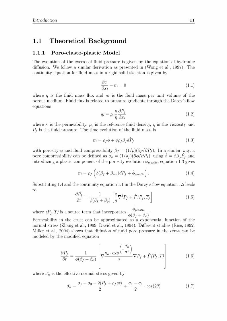
where ψ is the dilatancy angle.If we consider undrained porous materials, the effect of the fluid pressure is to shiftthe Mohr circle close to the failure envelop 1.1a. Then, undrained rocks could reachfailure at lower stresses than drained rocks. Using the idealization of two contact fric-tional surfaces, it is clear that the fluid pressure push the surfaces apart, diminishing

14 Introduction
the normal stress and promoting failure at lower stresses. When failure occurs inporous rocks, hydraulic parameters, mainly permeability, changes drastically (Davidet al., 1994; Zhang et al., 1999; Mitchell and Faulkner, 2008). This lead to localizedpore-fluid pressure increase and seepage forces become significant,(Rozhko et al.,2007). Then, the combine effect of seepage forces and the pore-fluid pressure in-crease is to change the radius of the Mohr circle while shifting it near to the failuresurface 1.1b. If nonlinear permeability is included, this effect is strong enough tocreate failure at lower pore-fluid pressures.
This mechanism is a principal factor in earthquakes triggering. It is known that theEarth crust is critically stressed and fluids can be in overpressurized pockets at depth.If these fluids are allow to scape, they will promote failure and failure creates fluidpaths allowing further fluid mobilization which may trigger more failure. This mightgenerate a self-sustained cycle of rock failure and fluid mobilization, an aftershocksequence.

Introduction 15
(a)
(b)
Figure 1.1: Mohr-Coulomb diagram. The blue line represent the Mohr-Coulomb failure envelop (shear failure). Green line is the Griffith cut off(tensile failure). (a) Homogeneous fluid pressure decreases the normalstress, moving the circle from initial position I to failure position II.(b) Localized pore fluid pressure changes the radius of the Mohr circlewhile shifting it near to the failure surface (position II). Lower pore fluidpressures might cause failure.
16 Introduction
1.2 Graphical Processing Units (GPUs) in Scien-
tific Numerical Modeling
1.2.1 GPU implementation of Poro-elasto-plastic Media
In nature, fracture networks are multiscale systems. Fractures lengths range fromcentimeters to kilometers long. Short fractures affects the background permeabilityof the rock, while large fractures, faults for example, work as main flow paths or flowchannels. The correct simulation of the fracture porous media should cast differentfracture length scales. This multiscality post problems from the point of view of nu-merical modeling. There are two main problems. First, the minimum fracture lengthin numerical models is given by the minimum length of the grid discretization, i.e.there is an “intrinsic fault length“ introduced by the numerical resolution and not bythe physics of the problem. All faults shorter than this “intrinsic fault length“ areconsider affecting only the background permeability. It is clear that the numericalresolution must be enough to resolve the minimum physical fractures length of theflow channels for the problem at hand. Second, if modeling of the fracture networkevolution is intent, then the numerical grid must be able to follow the developmentof new fractures and their propagation. A way to overcome this difficulty, couldbe to increase the numerical resolution in a specific “interesting area” or to remeshwhen new fractures develop. In realistic modeling of fractured porous media, manyfactors controls the fracture development. To determine an specific“interesting area”is problematic because nonlocalize fractures might develop creating unattached net-works. Under this circumstances, previous numerical zooming can not be accuratelyprescribed and constant remeshing is extremely computing expensive.
The approach that I use in this work is to fill the numerical domain with enoughpoints to resolve fractures down to a minimum length, which is small enough com-pared to the global scale of the problem. By doing so, the model is able to follow theevolution of the fracture network in the whole domain at every iteration. The maindrawback in this approach is the increment on the computation time. Implicit meth-ods would require the inversion of very large matrices and heavy matricial operationsthat require long computational time. I solved the problem using explicit finite dif-ference methods. Explicit methods has the advantage of being computationally lightbut time steps are very restrictive, increasing again the overall computation time.Parallel computation allows fast computation over large data sets. In particularGraphical Processor Units (GPU’s) have become a paradigm in parallel computingduring the last ten years.
The video games industry moves billions of dollars every year. Video games com-panies race to capture the favor of consumers introducing more realistic graphicsto increase the reality feeling in their products. This requires better software andhardware to be able to manage the amount of information per frame and the highvelocity frame rates. Real time, high resolution 3D graphics rendering, requires par-allel intensive computation over large data sets. In order to deal with this, GPU’s

Introduction 17
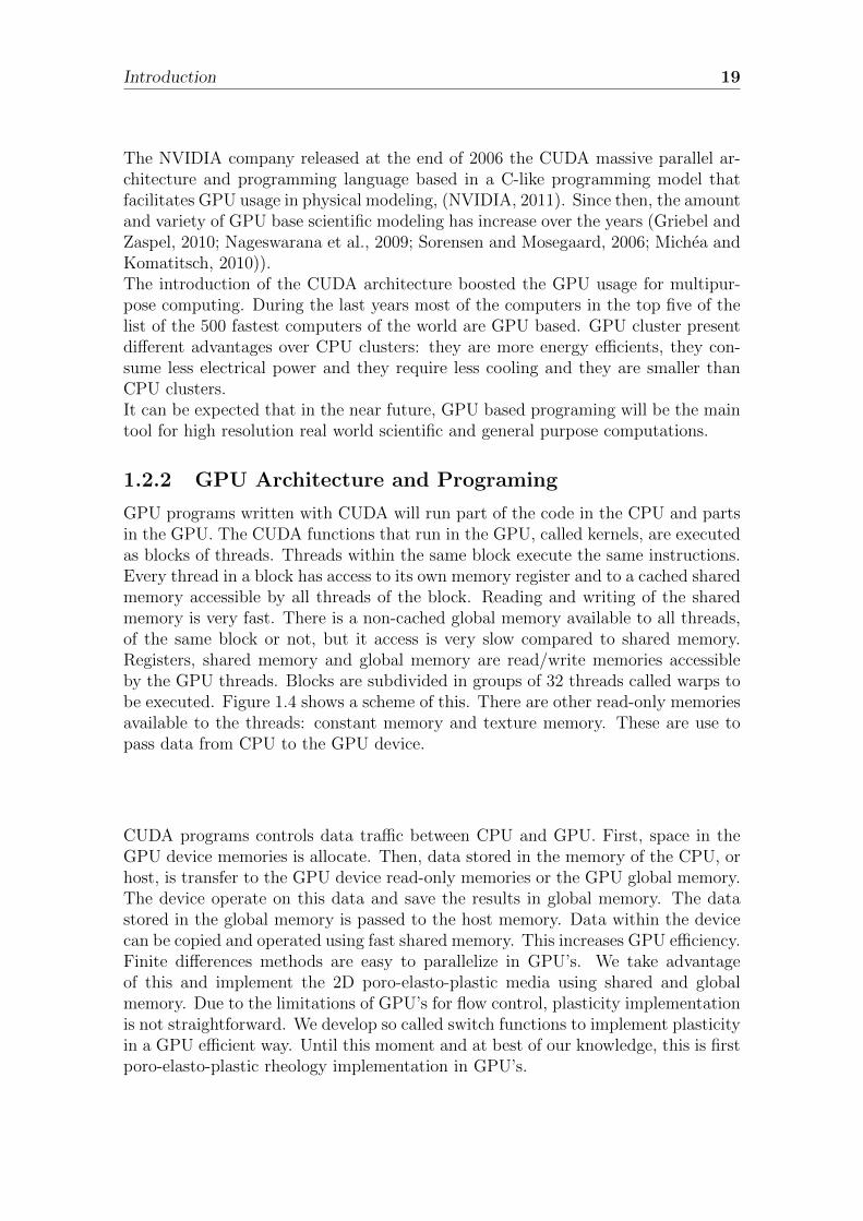
Figure 1.2: CPU architecture is designed for serial computations. Forthis reason it dedicates more chip space to flow control and memoryoperations. GPUS architecture gives priority to arithmetic intensiveoperations. Much more Arithmetic Logic Units (ALUs) are build inGPU chips.Cache memory for memory operations and flow control unitsare limited causing GPUs to be inefficient in comparison to CPUs forserial processes. From (NVIDIA, 2011).
architecture give more importance to data processing than to data catching or con-trol flow. This is done by including many of so called streaming processor cores,that execute the same instruction stream in parallel. Therefore, just a limited flowcontrol capacity is needed. Furthermore, streaming processor cores perform lightweight arithmetic operations over the data in an intensive way, i.e., much morearithmetic operations are performed as memory operations, making necessary justa limited cached memory. Figure 1.2 presents a comparison of the CPU vs GPUarchitectures. Then, GPU’s are well suited for problems that can be described in aparallel way in which single instructions operate over the whole data or large partsof the data.
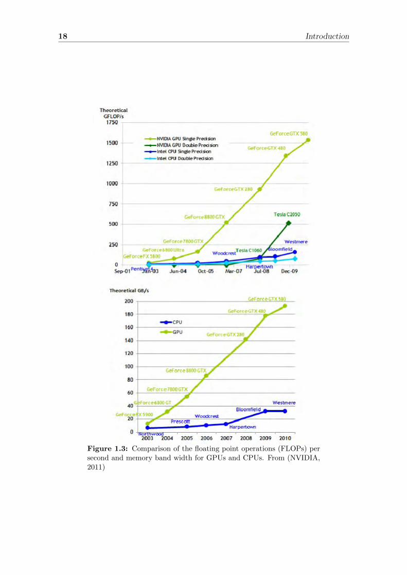
The difference in the performance of GPU vs CPU during the last year has grownexponentially. The number of floating points operations (FLOPs) per second in aGPU is orders of magnitude higher than a CPU Figure 1.3. This difference willnot decrease in the near future. Then, GPU’s can be efficiently used to acceleratenumerical applications if the most computing expensive parts of the code are pro-cessed on them while the memory management and control parts are executed usingCPU’s.
These capabilities were not overlook by the scientific community. Since its intro-duction in 1999, Graphics Processor Units (GPU) have been successfully appliedto accelerate non-graphical computations. Its applicability was strongly limited bythe complexity and limitations of the graphical programing languages available atthe moment. The use of these languages, as OpenGl, to nongraphical purposes wasa very difficult task. Nonetheless, some scientific applications were implemented.
18 Introduction
Figure 1.3: Comparison of the floating point operations (FLOPs) persecond and memory band width for GPUs and CPUs. From (NVIDIA,2011)
Introduction 19
The NVIDIA company released at the end of 2006 the CUDA massive parallel ar-chitecture and programming language based in a C-like programming model thatfacilitates GPU usage in physical modeling, (NVIDIA, 2011). Since then, the amountand variety of GPU base scientific modeling has increase over the years (Griebel andZaspel, 2010; Nageswarana et al., 2009; Sorensen and Mosegaard, 2006; Michea andKomatitsch, 2010)).The introduction of the CUDA architecture boosted the GPU usage for multipur-pose computing. During the last years most of the computers in the top five of thelist of the 500 fastest computers of the world are GPU based. GPU cluster presentdifferent advantages over CPU clusters: they are more energy efficients, they con-sume less electrical power and they require less cooling and they are smaller thanCPU clusters.It can be expected that in the near future, GPU based programing will be the maintool for high resolution real world scientific and general purpose computations.
1.2.2 GPU Architecture and Programing
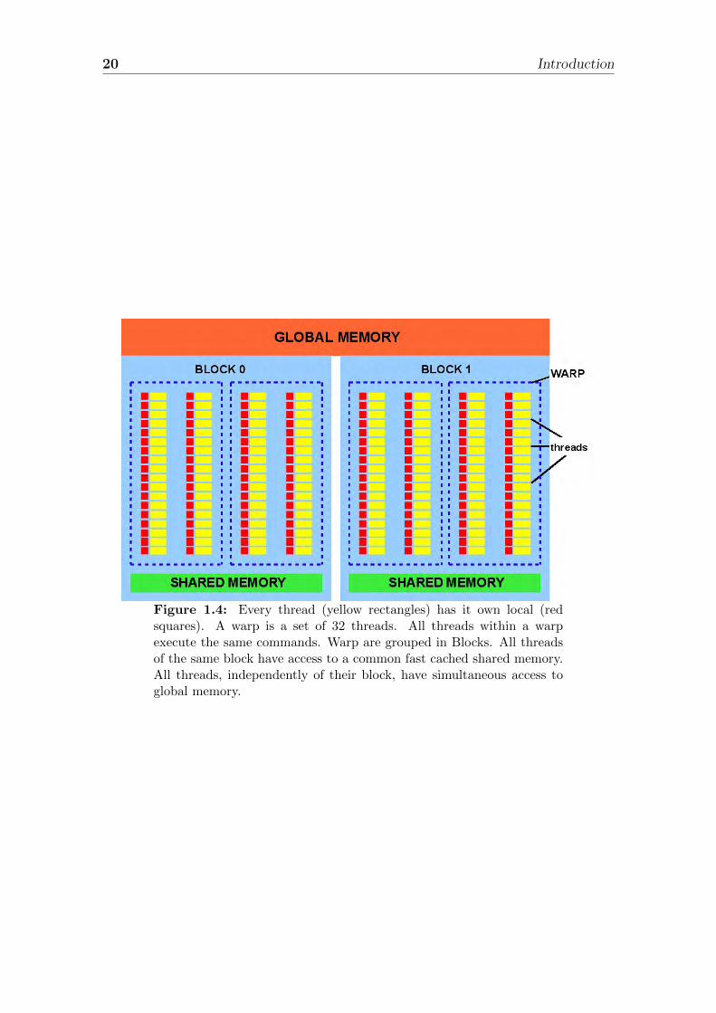
GPU programs written with CUDA will run part of the code in the CPU and partsin the GPU. The CUDA functions that run in the GPU, called kernels, are executedas blocks of threads. Threads within the same block execute the same instructions.Every thread in a block has access to its own memory register and to a cached sharedmemory accessible by all threads of the block. Reading and writing of the sharedmemory is very fast. There is a non-cached global memory available to all threads,of the same block or not, but it access is very slow compared to shared memory.Registers, shared memory and global memory are read/write memories accessibleby the GPU threads. Blocks are subdivided in groups of 32 threads called warps tobe executed. Figure 1.4 shows a scheme of this. There are other read-only memoriesavailable to the threads: constant memory and texture memory. These are use topass data from CPU to the GPU device.
CUDA programs controls data traffic between CPU and GPU. First, space in theGPU device memories is allocate. Then, data stored in the memory of the CPU, orhost, is transfer to the GPU device read-only memories or the GPU global memory.The device operate on this data and save the results in global memory. The datastored in the global memory is passed to the host memory. Data within the devicecan be copied and operated using fast shared memory. This increases GPU efficiency.Finite differences methods are easy to parallelize in GPU’s. We take advantageof this and implement the 2D poro-elasto-plastic media using shared and globalmemory. Due to the limitations of GPU’s for flow control, plasticity implementationis not straightforward. We develop so called switch functions to implement plasticityin a GPU efficient way. Until this moment and at best of our knowledge, this is firstporo-elasto-plastic rheology implementation in GPU’s.
20 Introduction
Figure 1.4: Every thread (yellow rectangles) has it own local (redsquares). A warp is a set of 32 threads. All threads within a warpexecute the same commands. Warp are grouped in Blocks. All threadsof the same block have access to a common fast cached shared memory.All threads, independently of their block, have simultaneous access toglobal memory.
Introduction 21
1.3 Summary of the Scientific Articles
In this section we present a resume of the three scientific articles produced duringthis work.
1.3.1 A full GPU simulation of evolving fracture networksin a heterogeneous poro-elasto-plastic medium witheffective-stress-dependent permeability
In the first paper I introduce the equations of poro-elasto-plastic media and the nu-merical schemes used to solve them. Then, GPU programming is introduced and thedifferent aspect for the poro-elasto-plastic media implementation in GPU are pre-sented. The main problem arise in the plasticity implementation. GPU’s have a verylimited capacity to handle point by point operations and conditions. The plasticitycomputation requires to evaluate the yield function and apply the computation ofplastic stresses for the specific points that fulfill the yield criteria. I develop so-calledswitch functions to handle the program branching. We present benchmarks of thedifferent parts of the code. The nonlinear diffusion solver is benchmarked using theMethod of Manufactured Solution (MMS) and is compared to a CPU implementa-tion. Then the elasto-plastic solver benchmarks are presented. Finally, we apply thecode to model fluid migration from a overpressurized layer at depth. Compressionaland extensional cases are analyzed. Extensional environments enhance the fluid mo-bilization and consequent failure. The results of this paper shows that aftershockssequences can be triggered and sustained due to fluid mobilization.
1.3.2 GPU numerical reproduction of hydrofracture exper-iments in Poro-elasto-plastic material
The main goal of this paper is to reproduce laboratory experiments of induced hy-drofracturing in critically stressed rocks. Simulation of laboratory experiments offluid infiltration in sandstone are used to calibrate the model. Using GPU technol-ogy we are able to model the system up to grain scales. It is shown that permeabilityplays and important role. We show an excellent correlation between model and ex-periment of the evolved fracture topology, as an indication that the model encompassthe underlaying physics.
1.3.3 Simulation of fluid induced seismicity accelerated inGPU. Application to Enhance Geothermal Systems
In this paper, I focus in the effects of fluid injection in highly fractured rock inrelation to Enhanced Geothermal Systems (EGS). I simulate a highly fractured rockmatrix in the vicinity of the borehole. Results of the simulation show that the usualassumption of keeping fluid injection pressure below the minimum compressive stressis not an adequate constraint to restrict hydrofracturing. We show that high damageoccurs far below this threshold.

22 Introduction
1.3.4 A poro-elasto-plastic model to simulate earthquake-volcano interaction dynamics in Central Chile
Here I applied the poro-elasto-plastic model to investigate earthquake-volcanic in-teractions in the Central Chile volcanic arc. The influence of the inter-seismic andpost-seismic regimes on the crust below the volcanic arc were modeled. It is shownthat the static extensive stresses of the post-seismic regime encourage the upwardmobilization of fluid through fractures. This process explains the time gap betweenearthquakes and volcanic erruptions.

Part II
PAPERS
23

Chapter 2
A full GPU simulation of evolvingfracture networks in aheterogeneous poro-elasto-plasticmedium witheffective-stress-dependentpermeability
2.1 Abstract
The wide range of timescales and underlying physics associated with simulatingporo-elasto-plastic media present significant computational challenges. GPU tech-nology is particularly advantageous to overcome these problems because even thoughthe physics are the same, computational times are orders of magnitude faster. Poro-elasticity could be implemented in GPU, however GPU implementation of plasticstresses pose problems because branching is introduced into the program and thusintroduces efficiency penalties. In general, any element by element evaluation todeal with branching in GPU is very inefficient. In this paper, we describe fractureevolution in a poro-elasto-plastic medium and use a switch on- switch-off function toavoid branching, allowing efficient computation of plasticity in GPU. We benchmarkfor the elasto-plastic part by investigating the angles of developed shear bands, andbenchmark the non-linear diffusion part of the code using the method of manufac-tured solutions. Model results are presented for fluid pressure propagation throughan elasto-plastic matrix subjected to compression, and another for extension. Theresults demonstrate how fluid flow is restricted in the compression case because ofthe load-induced low permeability, while fluid flow is encouraged in the extensionalcase because of the extension-induced high permeability. Code performance is ex-cellent in GPU, and we are able to runs months of simulation using time steps of afew seconds within a few hours. With this new algorithm, many problems of cou-ple fluid flow and the mechanical response can be efficiently simulated at very high
25
26 GPU simulation of poro-elasto-plastic medium
resolution.
2.2 Introduction
Triggering of earthquakes by high pressure fluids is well documented in enhancedgeothermal systems ((Haring et al., 2008),(Shapiro and Dinske, 2009),(Audin et al.,2002)) and natural environments ((Miller et al., 2004),(Bols and Nur, 2002),(Ohtake,1974)). Injection of over-pressurized fluids into fault zones reduces the frictional re-sistance, thus lowering of the shear stress necessary to failure (Terzaghi, 1923; Nur,1971). Documented cases of fluid-triggered or fluid-assisted earthquake sequencesinclude the Mw=6.3 1997 Colfiorito (Miller et al., 2004) and Mw=6.3 L’Aquila(Terakawa et al., 2010) earthquake sequences in Italy, and the 2004 Mw=6.8 Ni-igata earthquake in Japan (Sibson, 2007). Observations of direct fluid generated byearthquake slip have been reported for the 1995 Mw=7.2 Kobe (Japan) earthquake(Famin et al., 2008) where large volumes of CO2 were produced from temperature-induced decarbonization.
Although fluids and faulting have long been known to be an important part ofthe earthquake process, modeling the spatio-temporal evolution of such systems iscomputationally challenging primarily through the dynamical property of intrinsicpermeability. Namely, permeability can change by orders of magnitude over shorttimescales because of the switch to high permeability at the onset of slip (Millerand Nur, 2000). Here we take a modeling approach that combines poro-elasto-plastic model of (Rozhko et al., 2007) with a non-linear diffusion model ((Rice,1992; Miller et al., 2004)), where the non-linearity arises through an effective-stressdependence of the permeability. The solid deformation is modeled using the FLAC(Fast Lagrangian Analysis of Continua) algorithm with density scaling (Cundall,1982), which is coupled to the non-linear diffusion model using an explicit finitedifference algorithm with adaptive time-stepping.
In general, simulations over time scales of months (relevant for modeling fluid-drivenaftershock sequences) takes many hours to days of computation time. Reducing thenumerical resolution is the typical strategy to reduce the computational time, but inour case this would mean introducing unrealistically large intrinsic length scales forthe fractures. More importantly, natural fracture networks occur over a wide range ofsize scales, from centimeters to kilometers, so reduced resolution is not an affordablesacrifice. The advantage of Graphics Processor Unit (GPU) technology is that itallows much faster computations due to its inherent parallel architecture, allowingmuch shorter computational times while also increasing numerical resolution. GPUsare particularly powerful for solving governing equations that can be formulated intoexplicit finite difference algorithms, like for example our full GPU poro-elasto-plasticmodel with adaptive time stepping discussed below.
GPU simulation of poro-elasto-plastic medium 27
2.3 Model equations
Different studies ((Rice, 1992),(Miller et al., 2004)) shows that diffusion of fluid porepressure in the crust can be modeled using a nonlinear equation with permeabilitybeing an exponential function of stresses ((Zhang et al., 1999),(David et al., 1994))of the form
∂Pf∂t
=1
(βf + βφ)∇
κo · exp
(−σnσ∗
)
φ · η∇Pf + Γ (Pf ,T)
(2.1)
where σn is the effective normal stress given by
σn =σ1 + σ3 − 2(Pf + %fgz)
2+σ1 − σ3
2· cos(2θ) (2.2)
and Pf is the fluid overpressure, κo is the permeability at zero normal stress, σ∗ isa constant related to the degree of fracturing of the rock, ρf is the fluid density,η is the viscosity, φ is the porosity, βf is the fluid compressibility, βφ is the porecompressibility and Γ (P,T) is the source term.
The elastodynamic equations in their velocity-stress form describe the elastic re-sponse of the rock skeleton
∂Vx∂t
=1
ρ(∂σeffxx
∂x+∂σxy∂y
) (2.3)
∂Vy∂t
=1
ρ(∂σeffyy
∂y+∂σxy∂x
+ ρg) (2.4)
∂σxx∂t
= (λ+ 2µ)∂Vx∂x
+ λ∂Vy∂y
(2.5)
∂σyy∂t
= λ∂Vx∂x
+ (λ+ 2µ)∂Vy∂y
(2.6)
∂τxy∂t
= µ
(∂Vx∂x
+∂Vy∂y
)(2.7)
with µ and λ are the Lame constants, ρ is the density, vx and vz is the velocity vectorand σxx, σzz, τxz is the total stress tensor. In saturated porous rock, where the poresform a connected network, deformation is controlled by the Terzaghi effective stress
σeffij = σij − Pδij. (2.8)
Plastic deformation of rocks is modeled using Mohr-Coulomb and Griffith criteria
Ftension = τ − σm − σt (2.9)
Fshear = τ − σm · sin(ϕ)− C · cos(ϕ) (2.10)
F = max(Ftension, Fshear) (2.11)
28 GPU simulation of poro-elasto-plastic medium
where F is the yield function, ϕ is the internal frictional angle, τ is the stressdeviator, σm is the mean stress, σt is the tensile strength of the rock. The plasticstrain rates are given by
εplij = 0 for F < 0 or F = 0 and F < 0 (2.12)
εplij = λ∂q
∂σijfor F = 0 and F = 0. (2.13)
We use non-associative plastic flow rules (Vermeer and Borst, 1984)
qtension = τ − σm (2.14)
qshear = τ − σm · sin(ψ). (2.15)
In this report the dilatancy angle is ψ = 0. From linear theory of poroelasticity thefull strain tensor is given by
εij = εpeij + εplij (2.16)
where εelij is the poroelastic strain tensor. The poroelastic stress tensor is given by
σij = 2Gεpeij + 2Gεpekkν
1− 2νδij + αPfδij (2.17)
where α is the Biot-Willis constant, G is the shear modulus and ν is Poisson’s ratio((Jaeger et al., 2007),(Detournay and Cheng, 1993)).
2.3.1 GPU implementation
Since its introduction in 1999, Graphics Processor Units (GPU) have been suc-cessfully applied to accelerate non-graphical computations due to it highly parallelarchitecture. GPU implementations have been reported, to name a few, in fluiddynamics ((Griebel and Zaspel, 2010),(Zaspel and Griebel, 2011)), medical sciences((Nageswarana et al., 2009),(Sorensen and Mosegaard, 2006)) , geophysics ((Micheaand Komatitsch, 2010),(Lastra et al., 2009)), quatum chemistry (Vogt et al., 2008),molecular dynamics (Yang et al., 2007) and biology (Stivala et al., 2010). TheCUDA programming language, develop by NVIDIA and based in a C-like program-ming model, facilitates GPU usage in physical modeling, (NVIDIA, 2011).
GPU programs written with CUDA runs part of the code in the CPU and parts inthe GPU. The CUDA functions that run in the GPU are called kernels. The CPU,also refered as “host“ in GPU literature, handles the passage of the data to theGPU, called “device“ in GPU literature. The host has access to different memoriesof the GPU as the global memory, texture memories and constant memory. Fromthese memories the device can read the data and operate over it. The texture andconstant memories are read only memories for the device. The global memory isread/write memory type for the host and the device. The device has a second fastcached memory called shared memory. The global memory is non-cached and, inconsequence, slower. To increase the efficiency of a GPU code is preferable to use

GPU simulation of poro-elasto-plastic medium 29
Figure 2.1: Initial data matrices (a) of size nx × nz, are grouped together in large onedimensional vectors (b) of size number of matrices ·nz · nx to be passed to GPU.
shared memory for most of the computations. However , shared memory is verylimited in GPUs. To overcome this problem, the initial matrix of dimension nx×nzsaved in the global memory is subdivided in shared memory tessels and the deviceoperate with them.Kernels admit only a limited number of parameters. To avoid reaching this limit, theinitial data matrices (stresses, velocities, rheological properties, hydraulic properties,etc.) of size nx×nz, are grouped together into large one-dimensional vectors of sizenumber of matrices ·nz · nx to be passed to GPU. To access correctly different datasegments within the GPU matrices, we use the index expression:
index = x+ z ∗nx+ (position of the matrix in the large vector − 1) ∗nz ∗nx (2.18)
where x = 0 to nx− 1 and z = 0 to nz − 1.Figure 2.1 shows and sketch of this procedure.
We divide the problem in four main steps:
• solution of the nonlinear diffusion equation (2.17),
• computation of the effective stresses (2.8),
• solution of the velocities equations (3,4) and
• computation of the total stresses(5-7),
• evaluation of the yield function (2.9) and computation of plastic stresses using(2.12).
30 GPU simulation of poro-elasto-plastic medium
2.3.1.1 GPU nonlinear diffusion implementation
We use a first order in time, fourth order in space finite difference scheme to solve thenonlinear diffusion equation. Boundary conditions are zero flux boundary conditionsat the left, right and bottom edges and Dirichlet boundary conditions at the top,Pf = 0.We compute the solution of the nonlinear diffusion equation using shared mem-ory for the center of the domain and global memory for the boundary conditions.Two kernels perform the computation of the nonlinear diffusion: non lin diff andfluid diff write. First, nonlinear permeability is computed using equation 2.2 andthe new permeability is written to global and shared memories to be used in theequation 2.17. The inner part of the fluid pressure solution is computed using sharedmemory and the boundary conditions using global memory. The new fluid pressureprofile solution is written to a new position on the large GPU global memory ma-trices. We call this vector Pfnew. If the program tries to write the result directlyto the initial memory position, let us call it Pfinit, errors appears due to the factthat GPU tries to read and write the same memory address at the same time. Forthat reason, a second kernel fluid diff write writes the solution back to the initialrow vector Pfinit. A pseudocode of the kernels non lin diff and fluid diff write ispresented in algorithm tables 1 and 2.
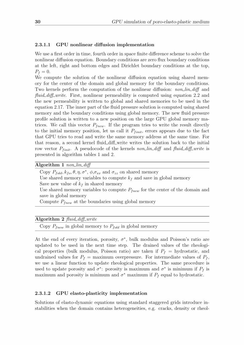
Algorithm 1 non lin diff
Copy Pfold, kfo, θ, η, σ∗, φ,σxx and σzz on shared memory
Use shared memory variables to compute kf and save in global memorySave new value of kf in shared memoryUse shared memory variables to compute Pfnew for the center of the domain andsave in global memoryCompute Pfnew at the boundaries using global memory
Algorithm 2 fluid diff write
Copy Pfnew in global memory to Pfold in global memory
At the end of every iteration, porosity, σ∗, bulk modulus and Poisson’s ratio areupdated to be used in the next time step. The drained values of the rheologi-cal properties (bulk modulus, Poisson ratio) are taken if Pf = hydrostatic, andundrained values for Pf = maximum overpressure. For intermediate values of Pf ,we use a linear function to update rheological properties. The same procedure isused to update porosity and σ∗: porosity is maximum and σ∗ is minimum if Pf ismaximum and porosity is minimum and σ∗ maximum if Pf equal to hydrostatic.
2.3.1.2 GPU elasto-plasticity implementation
Solutions of elasto-dynamic equations using standard staggered grids introduce in-stabilities when the domain contains heterogeneities, e.g. cracks, density or rheol-
GPU simulation of poro-elasto-plastic medium 31
ogy changes. To overcome this we use a staggered grid scheme with centered cells.Stresses were located in the cell centers and velocities on its corners. In the program,stresses have a size (nx+1)∗(nz+1) and velocities nx∗nz. However, all matrices arerearranged in the GPU to have size (nx+ 1)∗ (nz+ 1) by filling extra positions withzeros. Boundary conditions for stresses are zero slip at the right, left and bottomedges and free surface boundary condition at the top. Velocity boundary conditionsare vx = V and vz = 0 at the right edge, vx = −V and vz = 0 at the left edge andvz = 0 at the bottom.The kernel effective stresses computes equation 2.8. As in the case of the diffusion,the central part of the effective stress matrices is computed using shared memoryand boundary conditions using global memory. Table 3 present the pseudocode ofthis kernel. Velocities are computed in the kernel velocity computation using the
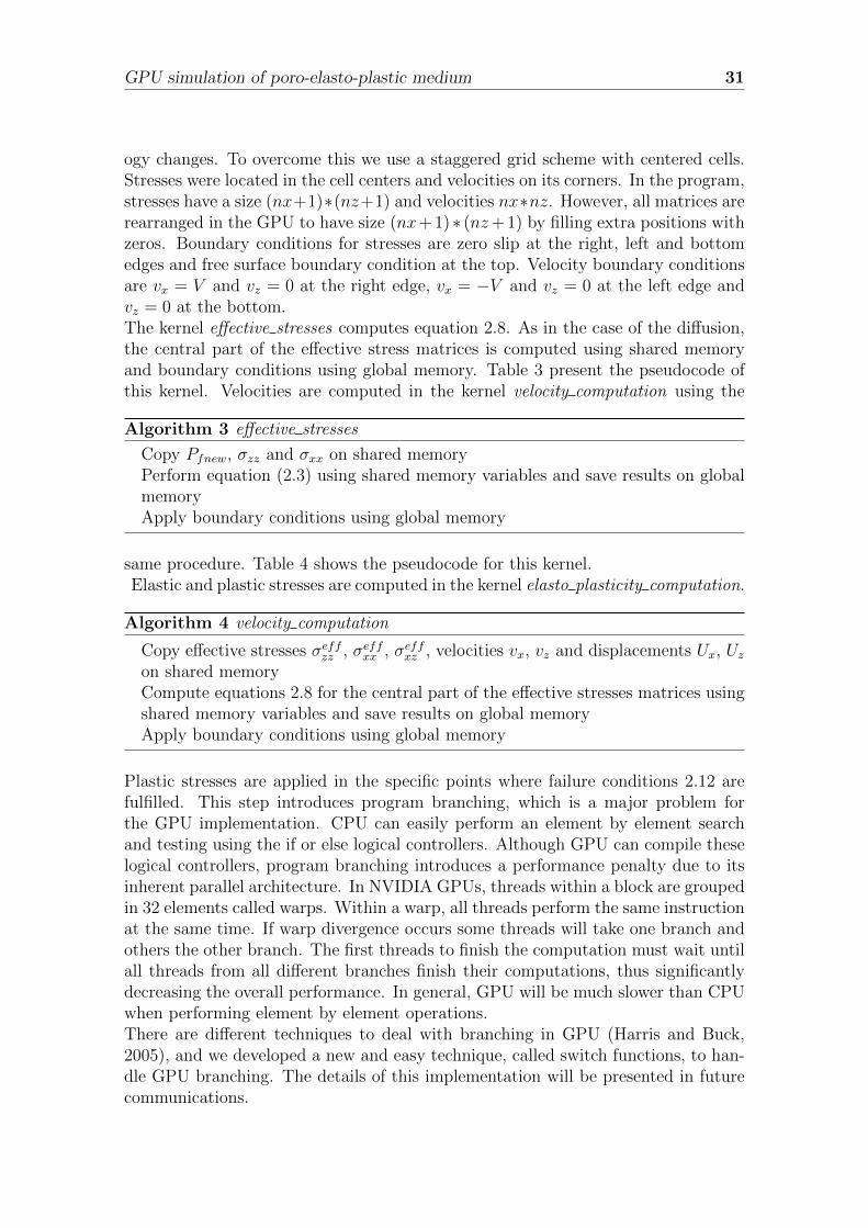
Algorithm 3 effective stresses
Copy Pfnew, σzz and σxx on shared memoryPerform equation (2.3) using shared memory variables and save results on globalmemoryApply boundary conditions using global memory
same procedure. Table 4 shows the pseudocode for this kernel.Elastic and plastic stresses are computed in the kernel elasto plasticity computation.
Algorithm 4 velocity computation
Copy effective stresses σeffzz , σeffxx , σeffxz , velocities vx, vz and displacements Ux, Uzon shared memoryCompute equations 2.8 for the central part of the effective stresses matrices usingshared memory variables and save results on global memoryApply boundary conditions using global memory
Plastic stresses are applied in the specific points where failure conditions 2.12 arefulfilled. This step introduces program branching, which is a major problem forthe GPU implementation. CPU can easily perform an element by element searchand testing using the if or else logical controllers. Although GPU can compile theselogical controllers, program branching introduces a performance penalty due to itsinherent parallel architecture. In NVIDIA GPUs, threads within a block are groupedin 32 elements called warps. Within a warp, all threads perform the same instructionat the same time. If warp divergence occurs some threads will take one branch andothers the other branch. The first threads to finish the computation must wait untilall threads from all different branches finish their computations, thus significantlydecreasing the overall performance. In general, GPU will be much slower than CPUwhen performing element by element operations.There are different techniques to deal with branching in GPU (Harris and Buck,2005), and we developed a new and easy technique, called switch functions, to han-dle GPU branching. The details of this implementation will be presented in futurecommunications.
32 GPU simulation of poro-elasto-plastic medium
2.4 Results
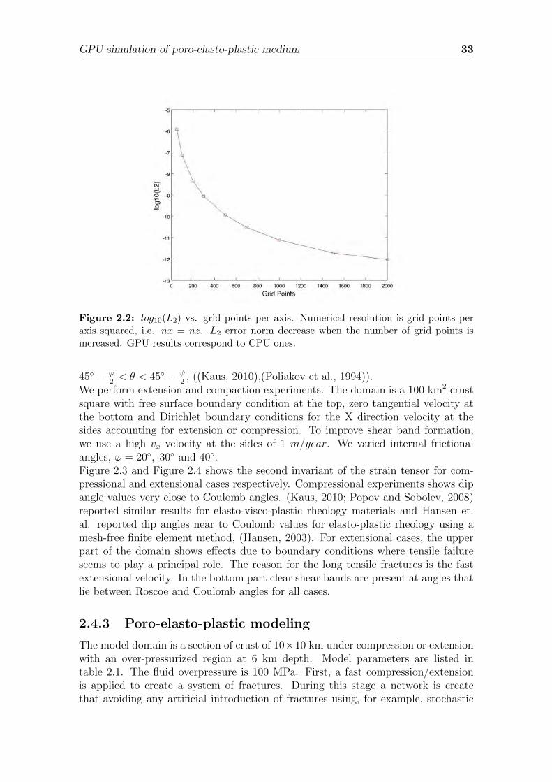
2.4.1 Nonlinear diffusion benchmark
The nonlinear diffusion algorithm was benchmarked using the Method of Manufac-tured Solutions (MMS),(Salari and Knupp, 2000). The MMS has been applied todifferent problems of computational fluid dynamics ((Bond et al., 2004),(Roy et al.,2004),(Shunn and Ham, 2007)). In this method, an artificial solution G is proposed.This solution does not need to be physically meaningful, but it must be smoothenough to be differentiable within the domain at the higher order of the differentialequation. The function G must not be a trivial solution of the differential equationand it must be complicated enough to test the accuracy of the numerical solution.A symbolic calculus software is used to differentiate the manufactured solution andthis result is compared to the numerical solution.The manufactured solution function is:
Pf = exp
−
(x− a)2
b+
(z − a)2
b
(2.19)
kfo = (0.1− 1−2 · z) · exp
−0.5 (σxx + σzz − 2 · Pf ) + 0.5 (σxx − σzz) cos (2 · θ)
σ∗
(2.20)
with a = 5, b = 25, σxx = σzz = 10 · z, σ∗ = 20 and θ = 60 and the domain ofthe function is Ω = x × z for x = [0, 10] and z = [0, 10]. These two functions aresmooth and their derivatives are continuous over this domain. We use the MATLABsymbolic calculus toolbox to compute the derivatives. We evaluate the equation
∇κo · exp
(−σnσ∗
)
η= RHS (2.21)
with η = 1, using the MATLAB symbolic calculus toolbox a CPU implementationand the GPU implementation. The L2 norm measures the global error between theanalytical, MATLAB symbolic solution, and numerical RHS . For all computationalexperiments grid points in X direction where equaled to grid points in Z, i.e. n =nx = nz. Grid points number per axis n was varied from 100 to 2000. Figure 2.2shows the results. Both implementations, CPU and GPU, converge to the analyticalsolution in the same way when the numerical resolution is increased.
2.4.2 Elasto-plastic benchmark
Elasto-plastic model benching is done by checking the formation of localized shearzones, shear bands, with the correct angle. There are three different theories thatdescribe the orientation of the shear bands: Coulomb, Roscoe and Arthur ((Arthuret al., 1977),(Bardet, 1990)). For a material with frictional angle ϕ and dila-tion angle ψ, shear bands form with dip angles θ between Rosco-Coulomb range,
GPU simulation of poro-elasto-plastic medium 33
Figure 2.2: log10(L2) vs. grid points per axis. Numerical resolution is grid points peraxis squared, i.e. nx = nz. L2 error norm decrease when the number of grid points isincreased. GPU results correspond to CPU ones.
45 − ϕ2< θ < 45 − ψ
2, ((Kaus, 2010),(Poliakov et al., 1994)).
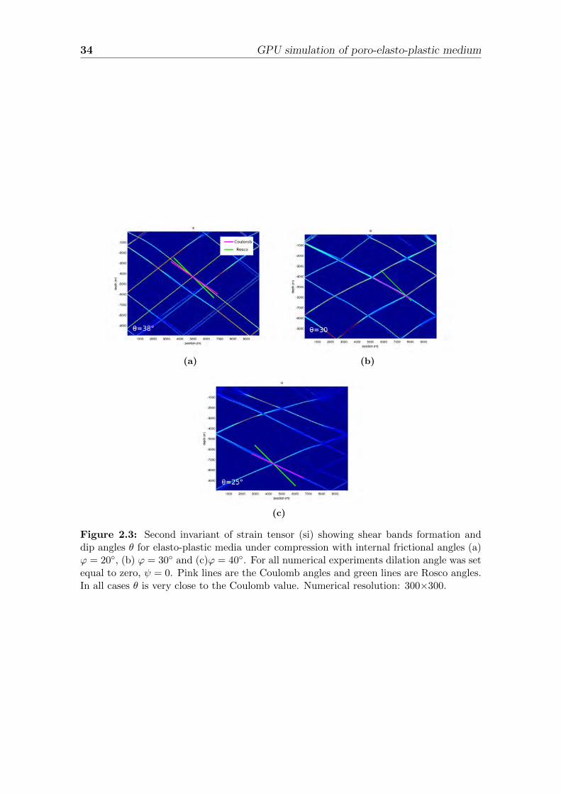
We perform extension and compaction experiments. The domain is a 100 km2 crustsquare with free surface boundary condition at the top, zero tangential velocity atthe bottom and Dirichlet boundary conditions for the X direction velocity at thesides accounting for extension or compression. To improve shear band formation,we use a high vx velocity at the sides of 1 m/year. We varied internal frictionalangles, ϕ = 20, 30 and 40.Figure 2.3 and Figure 2.4 shows the second invariant of the strain tensor for com-pressional and extensional cases respectively. Compressional experiments shows dipangle values very close to Coulomb angles. (Kaus, 2010; Popov and Sobolev, 2008)reported similar results for elasto-visco-plastic rheology materials and Hansen et.al. reported dip angles near to Coulomb values for elasto-plastic rheology using amesh-free finite element method, (Hansen, 2003). For extensional cases, the upperpart of the domain shows effects due to boundary conditions where tensile failureseems to play a principal role. The reason for the long tensile fractures is the fastextensional velocity. In the bottom part clear shear bands are present at angles thatlie between Roscoe and Coulomb angles for all cases.
2.4.3 Poro-elasto-plastic modeling
The model domain is a section of crust of 10×10 km under compression or extensionwith an over-pressurized region at 6 km depth. Model parameters are listed intable 2.1. The fluid overpressure is 100 MPa. First, a fast compression/extensionis applied to create a system of fractures. During this stage a network is createthat avoiding any artificial introduction of fractures using, for example, stochastic
34 GPU simulation of poro-elasto-plastic medium
(a) (b)
(c)
Figure 2.3: Second invariant of strain tensor (si) showing shear bands formation anddip angles θ for elasto-plastic media under compression with internal frictional angles (a)ϕ = 20, (b) ϕ = 30 and (c)ϕ = 40. For all numerical experiments dilation angle was setequal to zero, ψ = 0. Pink lines are the Coulomb angles and green lines are Rosco angles.In all cases θ is very close to the Coulomb value. Numerical resolution: 300×300.

GPU simulation of poro-elasto-plastic medium 35
(a) (b)
(c)
Figure 2.4: Shear band formation and dip angles θ for elasto-plastic media under ex-tension cases. Dilation angle ψ = 0 and frictional angles (a) ϕ = 20, (b) ϕ = 30 and(c)ϕ = 40. For all cases, dip angle θ lays between Roscoe (green line) and Coulomb (pinkline) angles. In the upper part of the domain tensile fracturing is appreciated. Numericalresolution: 300×300.
36 GPU simulation of poro-elasto-plastic medium
Parameter Hydrostatic pressure layer Overpressurized layerCohesion (MPa) 20 20
Poisson ratio 0.27 0.3Bulk modulus (GPa) 35 41
Porosity φ 0.01 0.10Intrinsic permeability κo (m2/s) 10−17 10−16
σ∗ (MPa) 33 35Pore compressibility βφ (Pa−1) 10−8 10−8
fluid compressibility βf (Pa−1) 10−10 10−10
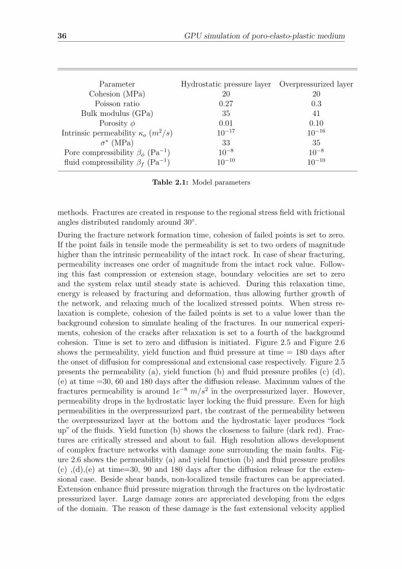
Table 2.1: Model parameters
methods. Fractures are created in response to the regional stress field with frictionalangles distributed randomly around 30.
During the fracture network formation time, cohesion of failed points is set to zero.If the point fails in tensile mode the permeability is set to two orders of magnitudehigher than the intrinsic permeability of the intact rock. In case of shear fracturing,permeability increases one order of magnitude from the intact rock value. Follow-ing this fast compression or extension stage, boundary velocities are set to zeroand the system relax until steady state is achieved. During this relaxation time,energy is released by fracturing and deformation, thus allowing further growth ofthe network, and relaxing much of the localized stressed points. When stress re-laxation is complete, cohesion of the failed points is set to a value lower than thebackground cohesion to simulate healing of the fractures. In our numerical experi-ments, cohesion of the cracks after relaxation is set to a fourth of the backgroundcohesion. Time is set to zero and diffusion is initiated. Figure 2.5 and Figure 2.6shows the permeability, yield function and fluid pressure at time = 180 days afterthe onset of diffusion for compressional and extensional case respectively. Figure 2.5presents the permeability (a), yield function (b) and fluid pressure profiles (c) (d),(e) at time =30, 60 and 180 days after the diffusion release. Maximum values of thefractures permeability is around 1e−8 m/s2 in the overpressurized layer. However,permeability drops in the hydrostatic layer locking the fluid pressure. Even for highpermeabilities in the overpressurized part, the contrast of the permeability betweenthe overpressurized layer at the bottom and the hydrostatic layer produces “lockup” of the fluids. Yield function (b) shows the closeness to failure (dark red). Frac-tures are critically stressed and about to fail. High resolution allows developmentof complex fracture networks with damage zone surrounding the main faults. Fig-ure 2.6 shows the permeability (a) and yield function (b) and fluid pressure profiles(c) ,(d),(e) at time=30, 90 and 180 days after the diffusion release for the exten-sional case. Beside shear bands, non-localized tensile fractures can be appreciated.Extension enhance fluid pressure migration through the fractures on the hydrostaticpressurized layer. Large damage zones are appreciated developing from the edgesof the domain. The reason of these damage is the fast extensional velocity applied
GPU simulation of poro-elasto-plastic medium 37
(a) (b)
(c) (d) (e)
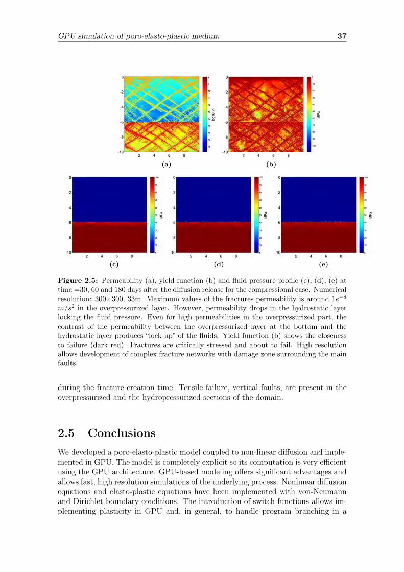
Figure 2.5: Permeability (a), yield function (b) and fluid pressure profile (c), (d), (e) attime =30, 60 and 180 days after the diffusion release for the compressional case. Numericalresolution: 300×300, 33m. Maximum values of the fractures permeability is around 1e−8
m/s2 in the overpressurized layer. However, permeability drops in the hydrostatic layerlocking the fluid pressure. Even for high permeabilities in the overpressurized part, thecontrast of the permeability between the overpressurized layer at the bottom and thehydrostatic layer produces “lock up” of the fluids. Yield function (b) shows the closenessto failure (dark red). Fractures are critically stressed and about to fail. High resolutionallows development of complex fracture networks with damage zone surrounding the mainfaults.
during the fracture creation time. Tensile failure, vertical faults, are present in theoverpressurized and the hydropressurized sections of the domain.
2.5 Conclusions
We developed a poro-elasto-plastic model coupled to non-linear diffusion and imple-mented in GPU. The model is completely explicit so its computation is very efficientusing the GPU architecture. GPU-based modeling offers significant advantages andallows fast, high resolution simulations of the underlying process. Nonlinear diffusionequations and elasto-plastic equations have been implemented with von-Neumannand Dirichlet boundary conditions. The introduction of switch functions allows im-plementing plasticity in GPU and, in general, to handle program branching in a
38 GPU simulation of poro-elasto-plastic medium
(a) (b)
(c) (d) (e)
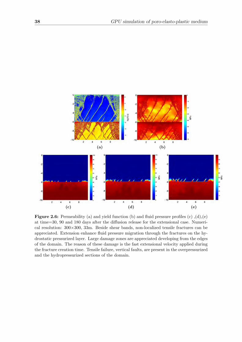
Figure 2.6: Permeability (a) and yield function (b) and fluid pressure profiles (c) ,(d),(e)at time=30, 90 and 180 days after the diffusion release for the extensional case. Numeri-cal resolution: 300×300, 33m. Beside shear bands, non-localized tensile fractures can beappreciated. Extension enhance fluid pressure migration through the fractures on the hy-drostatic pressurized layer. Large damage zones are appreciated developing from the edgesof the domain. The reason of these damage is the fast extensional velocity applied duringthe fracture creation time. Tensile failure, vertical faults, are present in the overpressurizedand the hydropressurized sections of the domain.

GPU simulation of poro-elasto-plastic medium 39
GPU efficient way.
Results of the code benchmarking are in accordance with previous studies. Theresults of the dip angles of shear bands of our model agrees with other numericalmodels. The Method of Manufactured Solutions (MMS) was used to benchmarkthe nonlinear diffusion equation giving accordance between CPU and GPU doubleprecision implementations.
The case of the full poro-elasto-plastic system under extension and compression werepresented. Complex fracture networks naturally develop from the stress conditions.Delocalized fractures, shear and tensile fractures can be appreciated. In the case ofcompression the fluids are ”lock” due to the decrease of the permeability. Extensionis favorable for fluid mobilization. Some of the aftershock sequences related to fluidlike the Colfiorito case (Miller et al., 2004) and L’Aquila (Terakawa et al., 2010)are extensional environments. This unlocking of the fluids has been proposed as atrigger factor in earthquake induced volcanic eruptions (Walter and Amelung, 2007).Due to the fast compressional and extensional velocities applied during the frac-ture creation large damage zones develop at the edges of the domain. Fracturingbegins at the edges. This effect can be diminished lowering the compressional andextensional velocities. A detail analysis of the evolution of the fracture network, itsgeometry, the permeability of the networks and behavior of the related parameters,will be done in the future. However, this work presents a model capable of developand handle very complex fluid-rock interactions.
This model can be used in different problems in geodynamics, e.g. effect of earth-quakes on permeability and fluid migration or to analyze hydrofracturing in engi-neering applications such as geothermal systems or oil and gas reservoir simulations.
To the best of our knowledge, this is the first implementation of poro-elasticity orplastic rheology in GPU. Due to complexity of our system its correct implementa-tion in GPU architecture opens by itself a new area of application for GPU basedmodeling. Developments of a 3D implementation of our model using GPU clusterswill be presented in the future.
2.6 Acknowledgments
We thank the German Research Foundation, Deutsche Forschungsgemeinschaft (DFG)for the financial support through the project no. MI 1237/2-1.

40 GPU numerical reproduction of hydrofracture experiments
Chapter 3
GPU numerical reproduction ofhydrofracture experiments inPoro-elasto-plastic material
3.1 Abstract
Modeling laboratory data at the scale of the experiment is extremely importantbecause if the model matches the observations at this small scale, then it meansthat the model captures the dominant underlying physics. Here I apply a numericalmodel of a pore-elastic plastic rheology coupled to non-linear diffusion to comparewith laboratory fluid injection experiments. The model is computed on the GPUplatform, allowing very high resolutions simulations of a continuum formulation atthe scale of the grain. We show an excellent correlation between model and experi-ment of the evolved fracture topology, providing strong indication that the dominantphysics are respected and modeled. I expect that additional future simulations ofwave propagation through the numerical samples will show equally good correlationswith measured changes in seismic velocities, or at least lead the way to further modelimprovements.
3.2 Introduction
Hydrofracturing is a common procedure for enhancing production of geothermalsystems or fossil fuel reservoirs. Tensile and shear fracturing can be achieved byinjecting high pressure water in the rock, which enhances permeability and thus thefluid flow within the hydrological system. If the rock is fractured, the injection ofhigh pressure fluids into fault zones reduces the frictional resistance, thus lowering ofthe shear stress necessary for failure (Terzaghi, 1923; Nur, 1971) and inducing seis-mic events. High pressure fluid-induced seismicity is well documented in enhancedgeothermal systems and hydrocarbon reservoirs (Majer et al., 2007; Haring et al.,2008; Shapiro and Dinske, 2009; Phillips et al., 2002; Audin et al., 2002; Glowackaet al., 1999), but modeling the underlying physics is complicated by the complex
41

42 GPU numerical reproduction of hydrofracture experiments
interactions between fluid flow, shear slip and changes in hydraulic properties at theonset of slip.In Enhanced Geothermal Systems (EGS), earthquakes are necessary to produce thepermeability enhancement, but these systems are typically near cities to make thisenergy source economically viable, so the magnitude of induced earthquakes is of sig-nificant concern. The public response and/or acceptance to induced seismic eventsis, in the end, a primary factor for the success or viability of a sustainable opera-tion. Two large European EGS projects, Soulz in France and the Deep Heat MiningProject Basel in Switzerland, were either suspended or cancelled because of publicoutcry to induced earthquakes (Haring et al., 2008; Majer et al., 2007). In the Baselexperiment, the strongest event had a magnitude of ML=3.4, which resulted in somestructural damage and ended that project.
Part of the problem with convincing the public is that few models exist that accu-rately describe these systems, so projections of what might be expected from induc-ing seismicity are restricted to statistical analyses or ’educated guesses’ of what willhappen. The purpose of this study is to develop a model that captures the domi-nant processes acting, namely fracture, pore-elastic stresses, and fluid flow and fluidpressure propagation associated with fluid injection. Our approach is to numericallymodel well-constrained laboratory experiments, and use those results to scale to thelarger EGS system.
There are a vast literature on laboratory experiments to analyze hydrofracturing.In a study of hydraulic fracturing in Weber sandstone (Lockner and Byerlee, 1977),where fluids were injected until sample failure, it was found that injection ratecontrols the failure mode of either shear or tensile failure. Typically geothermalreservoir systems are critically stressed to some degree, so particular efforts weremade in laboratory experiments under similar stress conditions. (Mayr et al., 2011;Stanchits et al., 2011) studied acoustic emissions (AE) in triaxial experiments ofcritically stressed Flechtingen sandstone during fluid injection, and showed thatrecorded cloud of acoustic emissions strongly correlated to the position of the waterfront.
Simulating geothermal reservoirs at the field scale requires that numerical modelshave been tested and calibrated at the high resolution scale of the laboratory. Thatis, numerical models should be able to reproduce laboratory scale experiments be-fore those same models can be used at the larger scale.In this paper, we present numerical results of a new, high resolution 2D poro-elasto-plastic code to reproduce recent experimental results of fluid injection into sandstone(Stanchits et al., 2011). Our model includes the effects of the deformation of the rockon the hydraulic properties and the fluid pressure feedback on the elastic propertiesof the rock, and we model the development, propagation, and interactions betweenevolving shear and tensile fractures. The following couplings are introduced: changesin the intrinsic permeability and cohesion due to fracturing, changes in the porosity,bulk modulus and Poisson’s ratio due to changes in the pore fluid pressure. Someproxies has been used to introduce this couplings. The numerical and experimental

GPU numerical reproduction of hydrofracture experiments 43
results show an excellent match between them.
We use CUDA programming of an explicit finite difference formulation of the govern-ing equations, and implement it on the Graphical Processing Unit (GPU) platform.GPU allows much faster computations due to its inherent parallel architecture athigh numerical resolution, and is particularly powerful for solving governing equa-tions that can be formulated into explicit finite difference algorithms, like for exampleour full poro-elasto-plastic model with adaptive time steppin discussed below. Inthis paper, we first review the equations of poro-elasto-plastic media, followed by abrief explanation of the numerical model and its GPU implementation. The numer-ical experiments are discussed and show a very good correlation with experimentalobservations.
3.3 Theoretical Model
Fluid pore pressure in the crust can be modeled using a nonlinear equation withan effective stress dependent permeability (Zhang et al., 1999; David et al., 1994;Rice, 1992; Miller et al., 2004). For laboratory scales the effective-stress-dependentpermeability and source terms can be negleted. With these assumptions the flowequation reduces to
∂Pf∂t
=1
η · (βf + βφ)∇κoφ∇Pf . (3.1)
where Pf is the fluid pressure, κo is the permeability intrinsic, η is the fluid viscosity,φ is the porosity, βf is the fluid compressibility and βφ is the pore compressibility.Thi equation accounts for changes int the porosity and intrinsic permeability. Asdiscussed later, the diffusivity κo increases by some amount when the failure occurs.The poro-elastic stress tensor is given by
σij = 2Gεpeij + 2Gεpekkν
1− 2νδij + αPfδij (3.2)
where α is the Biot-Willis constant, G is the shear modulus and ν is the Poisson’sratio ((Jaeger et al., 2007),(Detournay and Cheng, 1993)). These equations can belinked together using the Terzaghi effective stress as
σeffij = σij − αPδij. (3.3)
Plastic deformation of rocks can be modeled using Mohr-Coulomb and Griffith cri-teria
Ftension = τ − σm − σt (3.4)
Fshear = τ − σm · sin(ϕ)− C · cos(ϕ) (3.5)
F = max(Ftension, Fshear) (3.6)
where F is the yield function, ϕ is the internal frictional angle, τ is the stressdeviator, σm is the mean stress, σt is the tensile strength of the rock and C is the
44 GPU numerical reproduction of hydrofracture experiments
rock cohesion. The plastic strain rates are given by
εplij = 0 for F < 0 or F = 0 and F < 0 (3.7)
εplij = λ∂q
∂σijfor F = 0 and F = 0. (3.8)
We use non-associative plastic flow rules (Vermeer and Borst, 1984)
qtension = τ − σm (3.9)
qshear = τ − σm · sin(ψ). (3.10)
In this report the dilatancy angle is ψ = 0.
3.4 GPU implementation
Computation in graphical cards or Graphics Processor Units (GPU’s) has provenadvantageous for non-graphical purposes (Griebel and Zaspel, 2010; Zaspel andGriebel, 2011; Nageswarana et al., 2009; Sorensen and Mosegaard, 2006; Micheaand Komatitsch, 2010; Lastra et al., 2009; Vogt et al., 2008; Yang et al., 2007; Sti-vala et al., 2010). The CUDA programming language, introduced at the end of 2006by NVIDIA, has facilitated GPU usage in physical modeling, (NVIDIA, 2011).GPU’s substantially accelerate physical modeling because its architecture allows in-tensive parallel computation over large data sets by giving more importance to dataprocessing than to data cacheing or data control. This is accomplished by includingmany so-called streaming processor cores, that execute the same instruction streamin parallel. The streaming processor cores perform easy arithmetic operations inten-sively, i.e., it performs many more arithmetic operations than memory operations,limiting the amount of cached memory necessary. GPU’s are well suited for prob-lems that can be described in a parallel way, in which single instructions operateover the whole data or large parts of the data. Finite difference methods fall withinthis classification.GPU’s have three main write/read memory types: register, fast cached shared mem-ory and global uncached memory. We take advantage of this and implement the 2Dporo-elasto-plastic media using shared and global memory. To accelerate our codewe compute the central part of the domain using fast shared memory and boundaryconditions are computed using global memory. The correct memory managementresult in a fast, high-resolution efficient implementation.We use a first order in time, fourth order in space finite difference scheme to solve thenonlinear diffusion equation ??. To solve the elastodynamic equation 3.2 we use astaggered grid scheme with centered cells. Stresses are located in the cell centers andvelocities on its corners. At the end of every iteration, porosity, bulk modulus andPoisson’s ratio are updated using a linear function dependent on pore-fluid pressure.
GPU numerical reproduction of hydrofracture experiments 45
3.5 Numerical Model of Hydrofracturing in Tri-
axial Experiments
We test our numerical model by comparing our results to triaxial hydrofractureexperiments in Flechtingen sandstone reported by Stanchits et.al. and Mayr et.al.(Mayr et al., 2011; Stanchits et al., 2011). In their experiments, samples of 50 mmdiameter and 105-120 mm in length were subjected to confining pressures from 40-50MPa and loaded axially from 260 MPa until the critical stress of about 290 MPawas reached.We modeled two of their experiments, numbered Fb20 and Fb24. To be consistentwith their experiment names, we call our simulations NFb24 and NFb20 (N for nu-merical). In experiment Fb24, distilled water was injected from the bottom area ofthe sample with a pressure of 5.5 MPa, while in experiment Fb20, a borehole wasdrilled to approximately half the sample length into which fluid pressure of 5MPawas injected.
We use the viscosity at 25 , η = 8.9× 10⁻⁴ Pa/s and an the intrinsic permeabilityvalue for the intact rock is κo = 1 × 10⁻¹⁷ m2. To approximate the permeabilitychange due to fracturing, permeability was increased by one or two orders of magni-tude for shear and tensile fractures (David et al., 1994; Zhang et al., 1999; Mitchelland Faulkner, 2008). Because the model is pore-elastic, both drained and undrainedelastic constants are needed. Young’s moduli for drained Flechtingen sandstonesare in the range E=23.0-29.0 GPa with Poisson’s ratio ν = 0.12 (Backers, 2004).Undrained elastic constants are not available for Flechtingen sandstone, so we use theundrained elastic constant values determined for Ruhr sandstone because these havesimilar drained properties as the Flechtingen sandstone, Eu = 30 GPa , νu = 0.31,(Jaeger et al., 2007). The internal frictional angle is assumed being ϕ =35 degrees,and a tensile strength of σt = 6 MPa (Backers, 2004). We introduce some initial het-erogeneity by choosing cohesion values normally distributed around 20 MPa. Strainweakening was modeled reducing the cohesion of the failed points to zero. We as-sume porosity increases linearly from 0.055 at zero pressure to 0.15 at 5MPa withfluid pressure 2× 10⁻⁸Pa−1, with constant pore compressibility, therefore resultingin a range of storitivities. Additional detail of the laboratory experiments are foundin (Mayr et al., 2011; Stanchits et al., 2011). Model parameters are listed in Table 3.1
Our mesh resolution is 150×315 in the horizontal and vertical direction, respectively,resulting in a finite difference cell length of 0.333 × 10⁻³ m. The mean quartzgrain size of the Flechtingen sandstone is about 0.1−3 to 0.5−3m, so our continuumsimulation has the resolution of approximately the grain scale. The simulation timeis about 2 hours, and although we can not state the simulation time if this were runon CPU’s instead of GPU’s, our guess is that those simulations at this resolutionwould be on the order of 24 hours.We set the numerical confining pressure to 50 MPa and increase the the axial stressuntil the numerical rock is about to fail rock is about to fail by checking the maximumvalue of the yield function 3.4. For the simulation NFb20 the critical axial stress
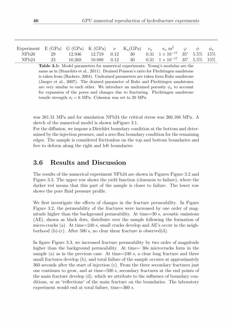
46 GPU numerical reproduction of hydrofracture experiments
Experiment E (GPa) G (GPa) K (GPa) ν Ku(GPa) νu κo m2 ϕ φ φuNFb20 29 12.946 12.719 0.12 30 0.31 1× 10⁻¹⁷ 35° 5.5% 15%NFb24 23 10.268 10.088 0.12 30 0.31 1× 10⁻¹⁷ 35° 5.5% 15%
Table 3.1: Model parameters for numerical experiments. Young’s modulus are thesame as in (Stanchits et al., 2011). Drained Poisson’s ratio for Flechtingen sandstoneis taken from (Backers, 2004). Undrained parameters are taken form Ruhr sandstone(Jaeger et al., 2007). The drained parameter of Ruhr and Flechtingen sandstonesare very similar to each other. We introduce an undrained porosity φu to accountfor expansion of the pores and changes due to fracturing. Flechtingen sandstonetensile strength σt = 6 MPa. Cohesion was set to 20 MPa
was 261.31 MPa and for simulation NFb24 the critical stress was 266.166 MPa. Asketch of the numerical model is shown inFigure 3.1.
For the diffusion, we impose a Dirichlet boundary condition at the bottom and deter-mined by the injection pressure, and a zero flux boundary condition for the remainingedges. The sample is considered frictionless on the top and bottom boundaries andfree to deform along the right and left boundaries.
3.6 Results and Discussion
The results of the numerical experiment NFb24 are shown in Figures Figure 3.2 andFigure 3.3. The upper row shows the yield function (closeness to failure), where thedarker red means that this part of the sample is closer to failure. The lower rowshows the pore fluid pressure profile.
We first investigate the effects of changes in the fracture permeability. In FigureFigure 3.2, the permeability of the fractures were increased by one order of mag-nitude higher than the background permeability. At time=30 s, acoustic emissions(AE), shown as black dots, distribute over the sample following the formation ofmicro-cracks (a). At time=240 s, small cracks develop and AE’s occur in the neigh-borhood (b)-(c). After 500 s, no clear shear fracture is observed(d).
In figure Figure 3.3, we increased fracture permeability by two order of magnitudehigher than the background permeability. At time= 30s microcracks form in thesample (a) as in the previous case. At time=240 s, a clear long fracture and threesmall fractures develop (b), and total failure of the sample occurrs at approximately360 seconds after the start of injection (c). From the three secondary fractures justone continues to grow, and at time=500 s, secondary fractures at the end points ofthe main fracture develop (d), which we attribute to the influence of boundary con-ditions, or as “reflections“ of the main fracture on the boundaries. The laboratoryexperiment would end at total failure, time=360 s.

GPU numerical reproduction of hydrofracture experiments 47
Figure 3.1: Setup for numerical hydrofracture experiments. Confiningstress is set at 50 MPa for both numerical experiments. The boreholein numerical experiment NFb20 is designated by the white lines. Axialstress for NFb20=261.31 MPa and pore fluid pressure Pf=5 MPa. Fornumerical experiment NFb24: axial stress was 266.166 MPa and fluidinjection pressure Pf=5.5 MPa. Samples are considered frictionless atthe top and bottom edges and at left and right edges are free to deform.
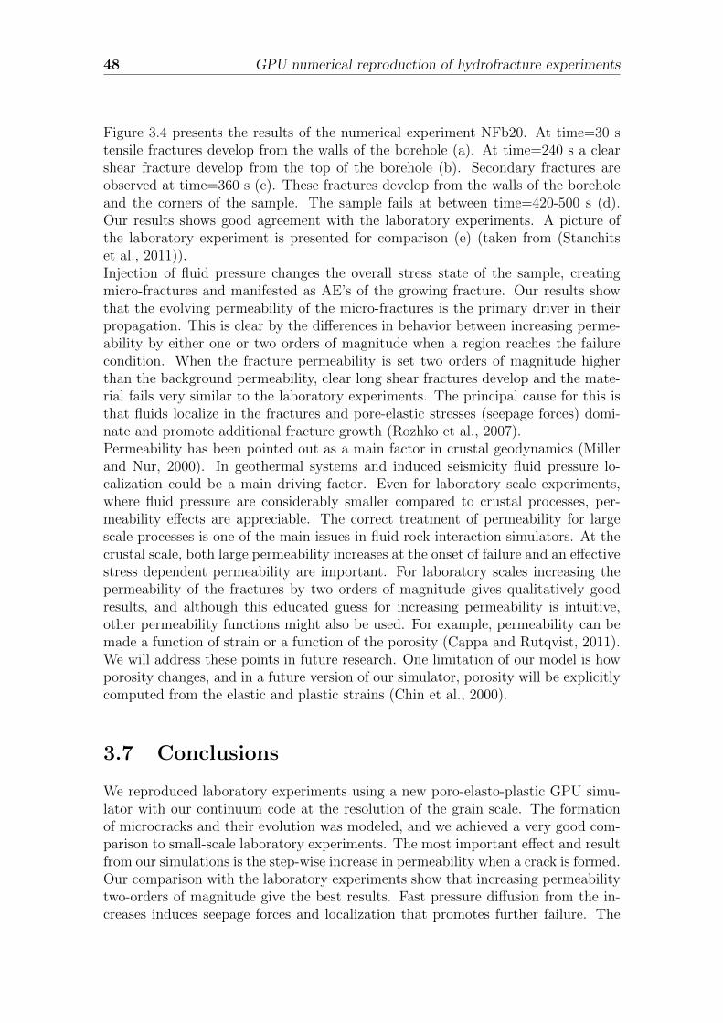
48 GPU numerical reproduction of hydrofracture experiments
Figure 3.4 presents the results of the numerical experiment NFb20. At time=30 stensile fractures develop from the walls of the borehole (a). At time=240 s a clearshear fracture develop from the top of the borehole (b). Secondary fractures areobserved at time=360 s (c). These fractures develop from the walls of the boreholeand the corners of the sample. The sample fails at between time=420-500 s (d).Our results shows good agreement with the laboratory experiments. A picture ofthe laboratory experiment is presented for comparison (e) (taken from (Stanchitset al., 2011)).Injection of fluid pressure changes the overall stress state of the sample, creatingmicro-fractures and manifested as AE’s of the growing fracture. Our results showthat the evolving permeability of the micro-fractures is the primary driver in theirpropagation. This is clear by the differences in behavior between increasing perme-ability by either one or two orders of magnitude when a region reaches the failurecondition. When the fracture permeability is set two orders of magnitude higherthan the background permeability, clear long shear fractures develop and the mate-rial fails very similar to the laboratory experiments. The principal cause for this isthat fluids localize in the fractures and pore-elastic stresses (seepage forces) domi-nate and promote additional fracture growth (Rozhko et al., 2007).Permeability has been pointed out as a main factor in crustal geodynamics (Millerand Nur, 2000). In geothermal systems and induced seismicity fluid pressure lo-calization could be a main driving factor. Even for laboratory scale experiments,where fluid pressure are considerably smaller compared to crustal processes, per-meability effects are appreciable. The correct treatment of permeability for largescale processes is one of the main issues in fluid-rock interaction simulators. At thecrustal scale, both large permeability increases at the onset of failure and an effectivestress dependent permeability are important. For laboratory scales increasing thepermeability of the fractures by two orders of magnitude gives qualitatively goodresults, and although this educated guess for increasing permeability is intuitive,other permeability functions might also be used. For example, permeability can bemade a function of strain or a function of the porosity (Cappa and Rutqvist, 2011).We will address these points in future research. One limitation of our model is howporosity changes, and in a future version of our simulator, porosity will be explicitlycomputed from the elastic and plastic strains (Chin et al., 2000).
3.7 Conclusions
We reproduced laboratory experiments using a new poro-elasto-plastic GPU simu-lator with our continuum code at the resolution of the grain scale. The formationof microcracks and their evolution was modeled, and we achieved a very good com-parison to small-scale laboratory experiments. The most important effect and resultfrom our simulations is the step-wise increase in permeability when a crack is formed.Our comparison with the laboratory experiments show that increasing permeabilitytwo-orders of magnitude give the best results. Fast pressure diffusion from the in-creases induces seepage forces and localization that promotes further failure. The
GPU numerical reproduction of hydrofracture experiments 49
(a) time=30 s (b) time=240 s (c) time=360 s (d) time=500 s
(e) time=30 s (f) time=240 s (g) time=360 s (h) time=500 s
Figure 3.2: Results of the numerical experiment NFb24 with fracturepermeability one order of magnitude higher than background permeabil-ity. First row shows the yield function or closeness to failure. Failureoccurs at yield function=0. Black dots are the acoustic emissions (AE’s).Second row is the pore fluid pressure profile. At time=30 s , AE’s (blackdots) of microcracks formation (a). At time=240-360 s shear cracks de-velop and AE’s occur around them (b)-(c). After 500 s there is no totalfailure but 5 long cracks are appreciable(d).

50 GPU numerical reproduction of hydrofracture experiments
(a) time=30 s (b) time=240 s (c) time=360 s (d) time=500 s
(e) time=30 s (f) time=240 s (g) time=360 s (h) time=500 s
Figure 3.3: Numerical experiment NFb24 with fracture permeabilitytwo order of magnitude higher than background permeability. At time=30s microcracks develop in the sample . At time=240 s a clear longfracture and three small fractures developed . Total failure of the sampleoccurred at approximately 360 seconds after injection is started .
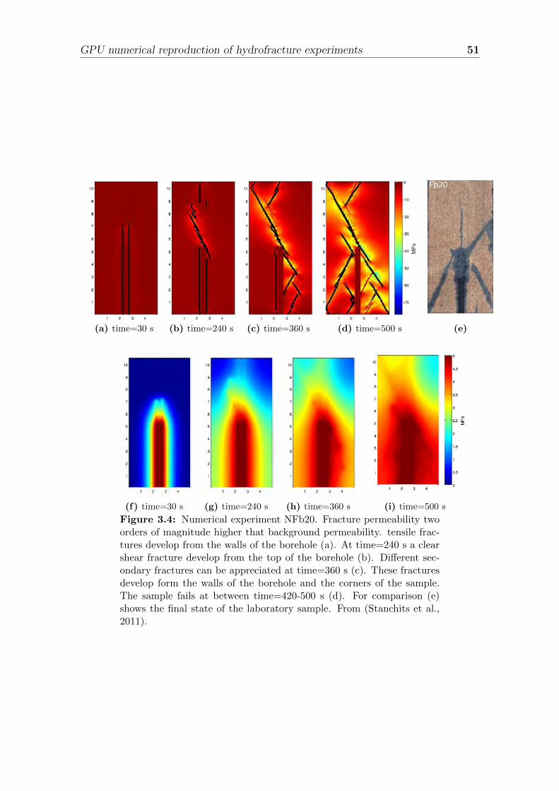
GPU numerical reproduction of hydrofracture experiments 51
(a) time=30 s (b) time=240 s (c) time=360 s (d) time=500 s (e)
(f) time=30 s (g) time=240 s (h) time=360 s (i) time=500 s
Figure 3.4: Numerical experiment NFb20. Fracture permeability twoorders of magnitude higher that background permeability. tensile frac-tures develop from the walls of the borehole (a). At time=240 s a clearshear fracture develop from the top of the borehole (b). Different sec-ondary fractures can be appreciated at time=360 s (c). These fracturesdevelop form the walls of the borehole and the corners of the sample.The sample fails at between time=420-500 s (d). For comparison (e)shows the final state of the laboratory sample. From (Stanchits et al.,2011).

52 GPU numerical reproduction of hydrofracture experiments
results presented shows that permeability is main factor in rock-fluid interactionsand these results, now calibrated against laboratory experiments, can now be appliedto larger scale systems such as enhanced geothermal systems. They are calibrationof our model for further developments and applications.
3.8 Acknowledgments
We thank Dr. Georg Dresen for personal communication during the preparation ofthis manuscript. We thank the German Research Foundation, Deutsche Forschungs-gemeinschaft (DFG) for the financial support through the project no. MI 1237/2-1.
Chapter 4
Simulation of fluid inducedseismicity accelerated in GPU.Application to EnhanceGeothermal Systems
4.1 Abstract
Injection of high pressure fluids into the earth is an important aspect of the futureof Green Energy. This includes Enhanced geothermal systems, CO2 sequestration,extraction of gas-shales and nuclear wast isolation. Here I apply a numerical modelof a pore-elastic plastic rheology coupled to non-linear diffusion to compare simu-late a generic EGS system and a direct application to the Basel, Switzerland, fluidinjection experiment. Results of the simulation show that the usual assumption ofkeeping fluid pressure below sigma 3 is not an adequate constraint to restrict hy-drofracture, because local heterogenity due to pore elastic effects and the evolvingfracture network result in local stress states permit hydrofracture by overcoming thelocal sigma 3 and not the far-field sigma 3. Once hydrofracture occurs even at asmall scale, the hydro-mechanical consequences of this local phenomenon, perturbthe overall future evolution the system and therefore its long-term viability.
4.2 Introduction
Geothermal energy is one of the candidates for a sustainable clean energy source forthe future. Thermal energy of the Earth is enough to satisfy the present and futureenergy needs of the society (Duffield and Sass, 2003).
In natural conditions, economically viable geothermal reservoirs must be located atdrillable depths, in water-saturated rocks with high porosity and conductivity attemperature high enough to produce steam or hot water at high enough flow rates.The places fulfilling these conditions are not widespread. However, hot-rock is avail-
53

54 Fluid induced seismicity in Poro-Elasto-Plastic media
able almost everywhere at drilling depths.
New techniques have been develop to use hot dry rock for the production of energy.For example, Enhanced Geothermal Systems (EGS) that are fractured, hot-rockreservoirs engineered to extract heat by the circulation of water (U.S.D.E, 2008).Permeability of poor geothermal systems could be enhanced by pumping water atpressure high enough to activate pre-existing fractures or creating new ones. EGSprojects has been implemented in the Geysers geothermal field in the U.S.A, CooperBasin in Australia, Berlın geothermal field in El Salvador, Soultz-sous-Forets inFrance and Basel in Switzerland (Majer et al., 2007). EGS are projected as a mainenergy source in the near future(U.S.D.E, 2008).
However, the induced microseismicity linked to the activation of fractures, is a mainissue for EGS projects as well as reservoirs exploitation (Ohtake, 1974; Majer et al.,2007; Haring et al., 2008; Shapiro and Dinske, 2009; Phillips et al., 2002; Audinet al., 2002). Generally, EGS projects are situated near to cities to avoid unneces-sary loss of heat during transportation and distribution of hot water. The publicresponse to induced seismicity, due to its frequency or magnitude, is a main fac-tor in EGS project operation. The last two EGS projects, Soultz-sous-Forets inFrance and Deep Heat Mining in Basel, Switzerland, have been either suspended oreven canceled due to public unrest caused by high seismicity. In the case of Soultz-sous-Forets high seismicity, with a large event of magnitude of 2.9 M, produced itstemporal suspension and in Basel high levels of seismicity, the largest even with amagnitude 3.4 ML, caused it cancellation (Majer et al., 2007; Haring et al., 2008).Is interesting that in both cases the largest event occurred after injection shut-in.
The last case, the Basel Deep Heat Mining (DHM) project deserve special atten-tion. In the DHM project the “safe” pumping fluid pressure was calculated to be74 MPa based in the inferred regional stress. However, pumping was stopped at apressure of approximately 29.6 MPa due to high seismicity. Computer simulation offractured geothermal systems might be a important tool to improve EGS planningand operation.
During the last years, many reports has been published about modeling of poro-elasto-plastic media and applications to geothermal systems (Chin et al., 2000;Taron et al., 2009; Taron and Elsworth, 2010), fluid induced seismicity,since pio-neering work of (Maillot et al., 1999) to (Shapiro et al., 2006; Baisch et al., 2010;Lupi et al., 2011) and CO2 sequestration (Xu et al., 2006; Rutqvist et al., 2007;Rutqvist et al., 2008; Cappa and Rutqvist, 2011).
Currently different fluid flow-heat flow-rock deformation simulators are available.For example GEOCRACK is a 2D simulator of fluid flow through fracture media. Itcouples deformation/fluid flow/heat flow. UDEC is 2D simulator that couples defor-mation and fluid flow, ROCMAS is a 3D finite element simulators of two phase flow(Rutqvist and Tsang, 2003), poroelasticity and thermoelasticity. FRACture is a fi-
Fluid induced seismicity in Poro-Elasto-Plastic media 55
nite elements poroelastic-thermoelastic simulator (Kohl et al., 1995). GeoSys/Rock-flow and its upgrade OpenGeoSys (Kolditz et al., ) are among the more complexsimulators nowadays . They are finite element 3D, multiphase flow, fracture flow,heat transport, chemical process, poroelastic, thermoelastic and elasto-plastic simu-lator (Wang and Kolditz, 2007). MOTIF (Model Of Transport In Fractured porousmedia) is a 3D finite element thermomechanical-groundwater flow-heat flow simula-tor (Guvanasem and Chan, 1995), FRANCON is finite element based 3D simulatorof thermo and poroelasticity and TOUGH-FLAC a heat flow-fluid flow-mechanicalsimulator with capabilities for elasto-plastic deformation. A more comprehensive listwith a brief description of the aforementioned codes is presented in (Rutqvist, 2011).
In most of these codes, fractures are treated as static or just small changes are pos-sible. For EGS and fracking, the description of the networks evolution is desirable.A realistic simulator, meant for these applications, must be able to create fracturesthat follow the regional stress conditions and the fractures must be able to changethe background stress introducing stress localization. Stress localization enhance theprobability of failure. Critically stressed fractures might yield even if just a very lowfluid pore pressure in injected. If fractures are introduced using stochastic methodsand they are not allow to evolve, the local stress field might be very different as theirregular stress field resulting from fracture evolution. This might lead to a wrong es-timation of the threshold for the injection pressure needed to control microseismicity.
Fractures change also the hydraulic parameters of the rock, mainly the permeabil-ity, that can increase orders of magnitude above the background rock permeability(David et al., 1994; Zhang et al., 1999; Mitchell and Faulkner, 2008). Fluids localizein fractures resulting in a highly inhomogeneous pore fluid pressure profile. Gradi-ents of pore fluid pressure introduces significant seepage forces that might promotemore failure (Rozhko et al., 2007).
In our numerical model, fractures are develop naturally from the local stress stateand they are free to evolve during the simulation. Complex networks and heteroge-neous stress fields are produced as a consequence.
To follow the fracture network evolution a very high numerical resolution is used.This process by itself would not give too much advantage because it represent longercomputational times and higher computer power. Using Graphics Processor Units(GPU) technology it is possible to reduce computation times and deal with largedata matrices (NVIDIA, 2011). GPU’s are highly parallel computation devices andhave been proven to be a solution for physical modeling when high resolution isrequired.We develop and efficient, high resolution poro-elasto-plastic simulator inGPU that allows fracture creation and evolution.
This paper is organized as following: in section 4.3 we review the equations of poro-elasto-plastic media. In section 4.4 we give a brief explanation of the GPU parallelarchitecture and programming. In 4.5 we present simulation of fluid injection in
56 Fluid induced seismicity in Poro-Elasto-Plastic media
fractured rock in the vecinity of the borehole and in 4.6 a real world case is mod-eled: the Basel DHM project. Finally section 4.7 present the conclusions.
4.3 Poro-elasto-plastic model
Stresses in fluid infiltrated rock are described by Biot poroelastic theory (Biot, 1941).The poroelastic stress tensor is defined as
σij = 2Gεpeij + 2Gεpekkν
1− 2νδij + αPfδij (4.1)
where α is the Biot-Willis constant, G is the shear modulus and ν is Poisson’s ratio.If an effective stress is defined as
σeffij = σij − Pδij (4.2)
equation 4.1 is identical to the stress equation for dry rock. Elastic strains arederived from equation 4.1 and force equations
∂Vx∂t
=1
ρ(∂σeffxx
∂x+∂σxz∂z
) (4.3)
∂Vz∂t
=1
ρ(∂σeffzz
∂z+∂σxz∂x
+ ρg) (4.4)
(4.5)
with ρ is the density, vx and vz is the velocity vector and σeffxx , σeffzz , τxz are theeffective stresses.Plastic yield of rocks can be modeled using Mohr-Coulomb and Griffith yield criteria
Ftension = τ − σm − σt (4.6)
Fshear = τ − σm · sin(ϕ)− C · cos(ϕ) (4.7)
F = max(Ftension, Fshear) (4.8)
where F is the yield function, ϕ is the frictional angle, τ is the stress deviator, σmis the mean stress, σt is the tensile strength of the rock. The plastic strain rates aregiven by
εplij = 0 for F < 0 or F = 0 and F < 0 (4.9)
εplij = λ∂q
∂σijfor F = 0 and F = 0. (4.10)
where q are the so called flow rules that describe the deformation of the materialin the plastic regime (Vermeer and Borst, 1984). Fluid pore pressure diffusion inthe crust can be model using a nonlinear diffusion equation with stress dependent

Fluid induced seismicity in Poro-Elasto-Plastic media 57
permeability (Gutierrez et al., 2000; Zhang et al., 1999; David et al., 1994; Rice,1992; Miller et al., 2004)
∂Pf∂t
=1
φ(βf + βφ)
∇κo · exp
(−σnσ∗
)
η∇Pf + Γ (Pf ,T)
(4.11)
where σn is the normal stress, Pf is the pore fluid overpressure, φ is the porosity, βfis the fluid compressibility, βφ is the pore compressibility, ρf is the fluid density, κo isthe permeability at zero normal stress, σ∗ is a scaling constant related to the degreeof fracturing of the rock, η is the viscosity. The last term in the right hand side ofthe equation 4.11 is the source term. For example, (Maillot et al., 1999) related thisterm to changes in the pore pressure due to compaction or extension of the solidmatrix. For the sake of simplicity we take the source term equal to zero in this report.
4.4 GPU implementation
In this Section we present a brief description of GPU’s architecture and program-ming. Refer to (NVIDIA, 2011) for more information.During the last 12 years Graphics Processor Units (GPU’s) have been used as acomputing platform for a manifold of physical models: fluid dynamics ((Griebel andZaspel, 2010),(Zaspel and Griebel, 2011)), geophysics ((Michea and Komatitsch,2010),(Lastra et al., 2009)), quantum chemistry (Vogt et al., 2008), molecular dy-namics (Yang et al., 2007) to name some. GPU’s development is boosted by thevideo game industry that requires rendering of high definition images at high speedframe rates, i.e. massive number of floating point operations per video frame. GPU’sare designed to execute massive number of threads. The company NVIDIA launchedin year 2006 the CUDA massive parallel architecture, together with its own program-ing language (NVIDIA, 2011). The CUDA language is C-like based and offers aneasier programing tool than former GPU graphic languages as OpenGl.GPU’s are composed of an array of streaming multiprocessor which of them contain-ing eight scalar processors (SP’s). In this report we use a GeForce GTX 590 NVIDIAGPU which has two graphic cards with 32 streaming multiprocessor in total. Besidescalar processor, each multiprocessor includes a multi-threaded instruction unit andcached memory. When a program calls a GPU kernel or function, many copies ofthis kernel are generated, called threads, and are passed to the GPU to be executed.The GPU distributes the threads among the available multiprocessors for execution.The multi-threaded instruction unit within each multiprocessor distribute, manage,schedule and execute threads using the so called single instruction multiple threads(SIMT) mode, i.e. the multiprocessor maps multiple threads, all of them repre-senting the same instruction, to the scalar processors to be execute. Threads areexecuted independently by the scalar processors. GPU’s can manage thousands of
58 Fluid induced seismicity in Poro-Elasto-Plastic media
threads simultaneously. Last generation GPU’s, as the GTX 590, can run 1536 si-multaneous threads for multiprocessor. This allows to crush large data set in pieces,accelerating operations over them. This approach is called single instruction multi-ple data (SIMD) parallelization.Threads are organized in blocks. Threads are accessible using a block index and athread index. Blocks are subdivided in groups of 32 threads called warp. When theGPU distributes the threads, it passes them to the multiprocessors as warps. Thenall threads within a warp execute the same instruction. The multiprocessor waitsuntil the execution of all threads of the current warps has been done before gettingthe next warp. If one of the threads diverges, the multiprocessor will wait until thatone is ready introducing a penalty in the efficiency.GPU’s have different memories types available to threads. Every thread in a blockhas access to its own memory register and to a cached memory shared by all threadsof the block. Reading and writing of the shared memory is very fast. There is anon-cached global memory available to all threads, of the same block or not, but itsaccess is very slow compared to shared memory (it access latency is approximately600 clocks cycles). To increase kernels efficiency most of the computation must beperform using shared memory. The register memory, shared memory and globalmemory are write/read memories. There are other read-only memories available forthe threads called constant memory and texture memory.Finite differences methods are well suited to parallelization in GPU’s. We imple-ment a first order in time, fourth order in space finite difference scheme to solve thenonlinear diffusion equation couple to a staggered grid scheme with centered cellsfor the elastodynamics equations. In both cases the central part of the domain iscomputed using shared memory and the boundary conditions using global memory.To implement the poro-elasto-plastic model in GPU we use a modular approach. Wesubdivide the problem in different kernels that can work independently of the others.We subdivide the problem in six main kernels: computation of nonlinear permeabil-ity, computation of nonlinear diffusion 4.11, computation of effective stresses 4.2,computation of velocities 4.3. The computation of poro-elastic stresses 4.1 , yieldfunction 4.6 and plastic strains 4.9 and plastic stresses is realized in one kernel.Finally a last kernel updates the rheological constants, porosity and σ∗ constant.Using this modular programing maintenance and further improvements of the codecould be implemented easier. Future improvements of our simulation include explicitcalculation of porosity and implementation of Gassmann equations for the rheolog-ical constants (Gassmann, 1951).
4.5 Fluid injection in heterogeneous fractured rock
First, the effect fluid injection in the vicinity of the borehole in highly fractured rockwas modeled. The model is an horizontal rock layer at 5 Km depth with a boreholein the middle. Maximum and minimum principal stresses act horizontal We modela 5 m×5 m squared layer with a borehole in the middle with a diameter of 30 cm.
Fluid induced seismicity in Poro-Elasto-Plastic media 59
The numerical grid had 500× 500 elements for numerical resolution of 1 cm.The pressure of the borehole is increased at rate of 1 MPa per hour from 1 MPauntil 99 MPa. Model parameters are presented in Table 4.1.
Parameter Value Units Definition
ρr 2540 kg m−3 Rock densityρw 971.8 kg m−3 Water densityKd 35 GPaKu 41 GPaνd 0.3νu 0.27ϕ 30 degrees Frictional angleG 18.9 GPa Shear modulus of the rockC 20 MPa Cohesion of the rockσt 10 MPa Tensile strength of the rockκdo 10−19 m2 Intrinsic background permeability for drained rockκuo 10−18 m2 Intrinsic background permeability for undrained rockκso 10−17 m2 Intrinsic permeability of shear fracturesκto 10−16 m2 Intrinsic permeability of tensile fracturesφd 0.01 Drained porosityφu 0.1 Undrained porosityφf 0.1 Fracture porosityσ∗d 35 MPa σ∗ for drained rockσ∗u 33 MPa σ∗ for undrained rockσ∗f 33 MPa σ∗ for fracturesβf 10−10 Pa−1 Fluid compressibilityβphi 10−8 Pa−1 Pore compressibility
Table 4.1: Parameters, symbols, values and units used for the numer-ical models. Taken from (Jaeger et al., 2007) and (Miller et al., 2004)
Rock anisotropy was modeled introducing a random variation on the frictional an-gle around 30 and on the cohesion around 20 MPa. Fracture network creation isachieved by compression applied at the left and right edges. Once the network isformed the stresses are relaxed towards the initial conditions. Figure 4.1 presentssome stages in the evolution of the fracture network. Upper row in Figure 4.1presents the yield function or closeness to failure (dark red is closer to failure).Black dots represent failing points at snapshot time. White circle represents theborehole position. Figure (a), (b) and (c) presents the initial, intermediate and finalstate of the network during stress relaxation time. Activation of different fracturescan be observed. In figure (a) activation of a non-optimal oriented fracture due toheterogeneity is appreciated at the top left side of the borehole. In figure (b) and
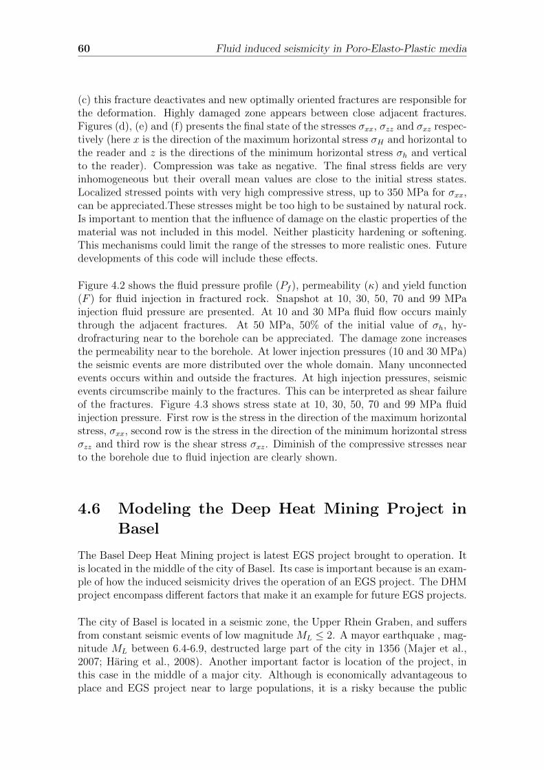
60 Fluid induced seismicity in Poro-Elasto-Plastic media
(c) this fracture deactivates and new optimally oriented fractures are responsible forthe deformation. Highly damaged zone appears between close adjacent fractures.Figures (d), (e) and (f) presents the final state of the stresses σxx, σzz and σxz respec-tively (here x is the direction of the maximum horizontal stress σH and horizontal tothe reader and z is the directions of the minimum horizontal stress σh and verticalto the reader). Compression was take as negative. The final stress fields are veryinhomogeneous but their overall mean values are close to the initial stress states.Localized stressed points with very high compressive stress, up to 350 MPa for σxx,can be appreciated.These stresses might be too high to be sustained by natural rock.Is important to mention that the influence of damage on the elastic properties of thematerial was not included in this model. Neither plasticity hardening or softening.This mechanisms could limit the range of the stresses to more realistic ones. Futuredevelopments of this code will include these effects.
Figure 4.2 shows the fluid pressure profile (Pf ), permeability (κ) and yield function(F ) for fluid injection in fractured rock. Snapshot at 10, 30, 50, 70 and 99 MPainjection fluid pressure are presented. At 10 and 30 MPa fluid flow occurs mainlythrough the adjacent fractures. At 50 MPa, 50% of the initial value of σh, hy-drofracturing near to the borehole can be appreciated. The damage zone increasesthe permeability near to the borehole. At lower injection pressures (10 and 30 MPa)the seismic events are more distributed over the whole domain. Many unconnectedevents occurs within and outside the fractures. At high injection pressures, seismicevents circumscribe mainly to the fractures. This can be interpreted as shear failureof the fractures. Figure 4.3 shows stress state at 10, 30, 50, 70 and 99 MPa fluidinjection pressure. First row is the stress in the direction of the maximum horizontalstress, σxx, second row is the stress in the direction of the minimum horizontal stressσzz and third row is the shear stress σxz. Diminish of the compressive stresses nearto the borehole due to fluid injection are clearly shown.
4.6 Modeling the Deep Heat Mining Project in
Basel
The Basel Deep Heat Mining project is latest EGS project brought to operation. Itis located in the middle of the city of Basel. Its case is important because is an exam-ple of how the induced seismicity drives the operation of an EGS project. The DHMproject encompass different factors that make it an example for future EGS projects.
The city of Basel is located in a seismic zone, the Upper Rhein Graben, and suffersfrom constant seismic events of low magnitude ML ≤ 2. A mayor earthquake , mag-nitude ML between 6.4-6.9, destructed large part of the city in 1356 (Majer et al.,2007; Haring et al., 2008). Another important factor is location of the project, inthis case in the middle of a major city. Although is economically advantageous toplace and EGS project near to large populations, it is a risky because the public

Fluid induced seismicity in Poro-Elasto-Plastic media 61
(a) (b) (c)
(d) σxx (e) σzz (f) σxzFigure 4.1: Evolution of the fracture network and final stress states. X and Zaxis in meters. Resolution 500×500, 1cm. Upper row presents the yield functionor closeness to failure (dark red is closer to failure). Black dots represent failingpoints at snapshot time. We relate these failing points to seismic events. Whitecircle represents the borehole position. Figures (a), (b) and (c) presents initial,intermediate and final state of the network during stress relaxation time. Activationof different fractures can be observed. In figure (a) activation of a non-optimaloriented fracture due to heterogeneity is appreciated at the top left side of theborehole. In figure (a) and (a) this fracture deactivates and new optimally orientedfractures are responsible for the deformation. Highly damaged zone appears betweenclose adjacent fractures. Figures (d), (e) and (f) presents the final state of the stressesσxx, σzz and σxz respectively (here x is the direction of the principal horizontal stressσH and horizontal to the reader and z is the directions of the minimum horizontalstress σh and vertical to the reader). Compression was take as negative. The finalstress fields are very inhomogeneous but their overall mean values are close to theinitial stress states. Localized stressed points with very high compressive or extensivestresses can be appreciated.
62
Fluid
inducedseismicityin
Poro-Elasto-Plastic
media
Pf=10 MPa Pf=30 MPa Pf=50 MPa Pf=70 MPa Pf=99 MPa
κ
F
Figure 4.2: Fluid injection pressure (Pf ), permeability (κ) and yield function (F )for fluidinjection in fractured rock. X and Z axis in meters. Snapshot at 10, 30, 50, 70 and 99 MPainjection fluid pressure are presented. At 10 and 30 MPa fluid flow occurs mainly through theadjacent fractures. At 50 MPa, 50% of the initial value of σh, hydrofracturing near to theborehole can be appreciated. The damage zone increases the permeability near to the borehole.At lower injection pressures (10 and 30 MPa) the seismic events are more distributed over thewhole domain. Many unconnected events occurs within and outside the fractures. At highinjection pressures, seismic events circumscribe mainly to the fractures. This can be interpretedas shear failure of the fractures.

Fluid
induced
seismicity
inPoro-E
lasto-Plastic
media
63
σxx
σzz
σxz
Figure 4.3: Stress state at 10, 30, 50, 70 and 99 MPa fluid injection pressure.X and Z axis inmeters. First row is the stress in the direction of the maximum horizontal stress, σxx, secondrow is the stress in the direction of the minimum horizontal stress σzz and third row is the shearstress σxz.
64 Fluid induced seismicity in Poro-Elasto-Plastic media
might be unrested by seismicity. For a large city as Basel, where other industriessettle, population might be alarm about the effects of seismicity in other economicalactivities. Besides, if the population is not directly dependent on the geothermalenergy its willingness to accept ground shaking will be low. It is necessary to in-form the public about the seismicity risk and expected ground movement. Realisticnumerical models might give answers to these questions allowing an more accurateplaning and seismic risk management as well as presenting to the public informationeasy to visualize and understand.
The DHM project gain relevance in December 2006 during it test time due to thetriggering of seismic events felt by the population, during approximately two monthsafter it operation start. In fact, the high levels of the seismicity lead the authoritiesto stop the project just 6 days after the initiation of the water injection. The biggestevent had a magnitude of ML =3.4. The project was canceled in the year 2009.The Basel 1 well was drilled through 2507 m of sedimentary rocks and 2493 m ofgranite basement to a maximum depth of 5000 m, with the open hole section begin-ning at 4629 meters. The diameter of the well in the open section is 8.5 inches or21.6 cm. We model a layer of 500×500 m at 4800 meters depth.
In Basel area the maximum and minimum principal compressional stresses lays on aplane almost horizontal, i.e., σ1 = σH and σ3 = σh. The intermediate compressional
stress is the overburden, σ2 = σV . The stress ratio R =σH − σ2σH − σ2
= 0.36 was inferred
by (Terakawa et al., 2012). With this R value one can choose the initial value of thestresses σH = 160 and σh = 65 at 4800 m depth. Heterogeneities are introduced inthe frictional coefficient taking normally distributed values around 0.7 and varyingfrom 0.58<µ<0.83 and similarly for the cohesion, taking values around 20 MPa. Wemodel a layer of 500m2 because most of the microseismic activity happen withinthis radius surrounding the free section of the injection well. All other elastic andhydraulic parameters are the same as the ones presented in Table 4.1.
The numerical grid has dimensions 2000×2000 for a numerical resolution of 25 cm.This very high resolution allows us to follow the evolution of the fractured networkvery accurately. This was near to the maximum resolution possible in our GPU card.
We create a fractured network by compressing the layer till fracturing. Figure showssome snapshot of the fracturing creation process. Figure shows the stress pattersafter the fracture creation time and the yield function signalizing closeness to frac-turing. Initial stresses are recover by relaxing the stresses back to the initial values.During the relaxation time further fracturing is produced. FIGURE shows the frac-tured network and stresses after the relaxation time. The resulting stress is veryinhomogeneous showing fracture localization and critically stressed fractures. How-ever, the mean value of R is around 0.36 fulfilling the initial stress conditions.round 0.36 fulfilling the initial stress conditions.
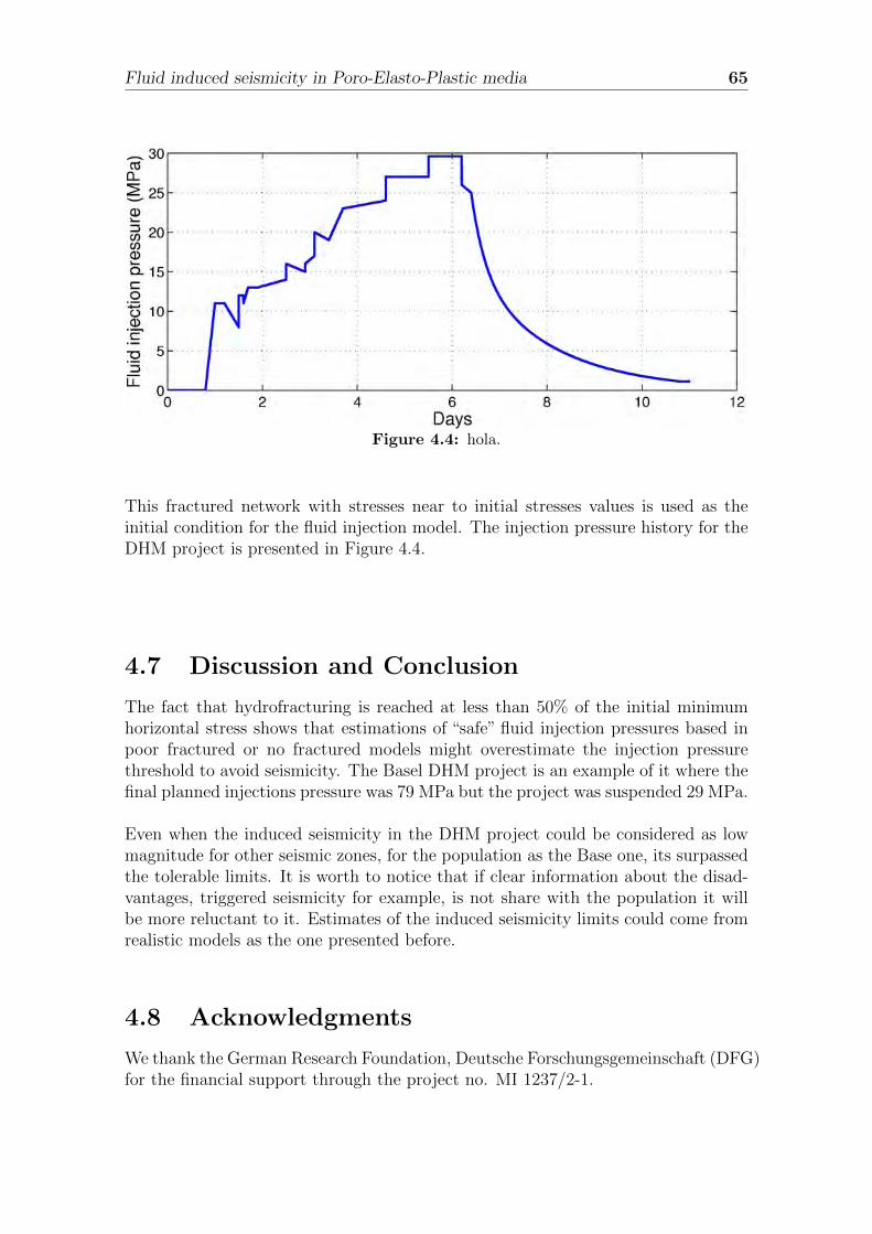
Fluid induced seismicity in Poro-Elasto-Plastic media 65
Figure 4.4: hola.
This fractured network with stresses near to initial stresses values is used as theinitial condition for the fluid injection model. The injection pressure history for theDHM project is presented in Figure 4.4.
4.7 Discussion and Conclusion
The fact that hydrofracturing is reached at less than 50% of the initial minimumhorizontal stress shows that estimations of “safe” fluid injection pressures based inpoor fractured or no fractured models might overestimate the injection pressurethreshold to avoid seismicity. The Basel DHM project is an example of it where thefinal planned injections pressure was 79 MPa but the project was suspended 29 MPa.
Even when the induced seismicity in the DHM project could be considered as lowmagnitude for other seismic zones, for the population as the Base one, its surpassedthe tolerable limits. It is worth to notice that if clear information about the disad-vantages, triggered seismicity for example, is not share with the population it willbe more reluctant to it. Estimates of the induced seismicity limits could come fromrealistic models as the one presented before.
4.8 Acknowledgments
We thank the German Research Foundation, Deutsche Forschungsgemeinschaft (DFG)for the financial support through the project no. MI 1237/2-1.

66 Something Volcanoes

Chapter 5
A poro-elasto-plastic model tosimulate earthquake-volcanointeraction dynamics in CentralChile
5.1 Abstract
The mechanism by which volcanoes respond to large magnitude earthquakes is stillstanding as one of the main question marks in geosciences. One possible explana-tion is a link to megathrust earthquakes whereby co- and post seismic volumetricexpansion of the upper plate facilitates the vertical migration of deep fluids. Tostudy how the 2010 M8.8 Maule earthquake, Chile, affected the nearby volcanic arc,we developed a poro-elasto-plastic model of the upper continental crust. The modelincludes the dependence of the permeability on the normal stresses in which eachseismic phase affects the fluid mobilization. Our simulations show how the post-seismic volumetric expansion of the upper crust alters the overall geological system,inducing creation and unclogging of fractures and promoting vertical migration ofdeep fluids. We provide an explanation of the time lap between megathrust earth-quakes and volcanic eruptions base on the constrains that poro-elasto-plastic effectsimpose on the crust permeability and the fluid mobilization through fractures.In this study we use the new GPU based code named eFrackTurbo to simulate thefluid-rock interactions related to earthquakes triggered volcanic eruptions.
5.2 Introduction
Volcanic response to seismic activity is a very well know phenomenon. Charles Dar-win described activity of different volcanoes following the 1835 M8.5 Conceptionearthquake, Chile (Darwin, 1840) . Cases of seismically induced volcanic activitywith varying time- and space-scales has been reported around the globe (Eggert and
67

68 Something Volcanoes
Walter, 2009). Examples of volcanic activity induced by large magnitude earth-quakes occurred in the USA (Sanchez and McNutt, 2004), Kamchatka (Walter,2007), Japan (Koyama, 2002), and Italy (Sharp et al., 1981; Nostro et al., 1998;Nercessian et al., 1991). Volcanic activity can be triggered by dynamic or staticstress variations. The first operate over short (hours to days) timescales while thesecond over long (months to years) timescales. The perturbation of the systeminduced by dynamic and stress triggering can reach 1/r1.66 and 1/r3, respectively,where r is the distance from the earthquake epicenter (Hill et al., 2002).
Cases of induced volcanism over short timescales are, for example, documented inKamchatka and Chile. Following the 1952 M9.0 Kamchatka earthquake (Johnsonand Satake, 1999) the Karpinsky and the Tao-Rusyr volcanoes began to erupt oneand seven days after the main shock, respectively (Walter and Amelung, 2007).Evidence of volcanic activity following the M8.1 1835 Concepcion, earthquake (Dar-win, 1840; Lara et al., 2004) includes eruptions of the Minchinmavida and CerroYanteles volcanoes less than 24 hours after the main shock (Darwin, 1840). Simi-larly, the Cordon Caulle volcano erupted less than two days following the M9.5 1960Valdivia earthquake (Lara et al., 2004). Other examples are the volcanoes Talang,Frafatoa and Tangkubanparahu in Indonesia that erupted two days after a M6.7aftershock approximately three months after the December 26, 2004, M9.3 Sumatraearthquake(Manga and Brodsky, 2006). Several mechanism have been suggestedto explain the dynamic propagation of stress. For instance, (Walter and Amelung,2007) suggest that at short (elastic) timescales, large slip on the subduction inter-face induces volumetric expansion in the upper plate, leading to magma mobilization(Amelung et al., 2007). Moreover, the passage of body and surface seismic waves(Hill et al., 2002; Walter and Amelung, 2007) can induce processes such as rectifiedgas diffusion (Manga and Brodsky, 2006), which will ultimately enhance upwelling ofdeep fluids and volatile exsolution (Sparks and Sigurdsson, 1977; Manga and Brod-sky, 2006).
However, the time lap between earthquakes and volcanic activity can extend to yearsdependent on the hypocentral distance to the volcanic system (Eggert and Walter,2009). For example, a M8.3 subduction earthquake in 1923 in Far East Russia trig-gered volcanic activity in Kamchatka with many different volcanoes erupting: twoin 1923, one in 1925, two in 1926, and one each in 1927, 1928, 1929 and 1930. Sim-ilarly, (Eggert and Walter, 2009) points out that the 1928 M7.6 Talca earthquake,Chile, was followed by large eruptions of the Quizapu-Cerro Azul (1932) and Dez-cabezado Grande (1933) volcanoes, which reside along the arc directly behind theTalca earthquake epicenter.
These megathrusts earthquakes induce static stress variations that can lead tocrustal deformation that relax the pre-earthquake regime (Eggert and Walter, 2009)and initiate long-duration extensional or transtensional tectonic regimes (Walter andAmelung, 2007) finally leading to permanent changes in the state of the volcanic sys-tems. This would explain the time gap of months to years between earthquake and
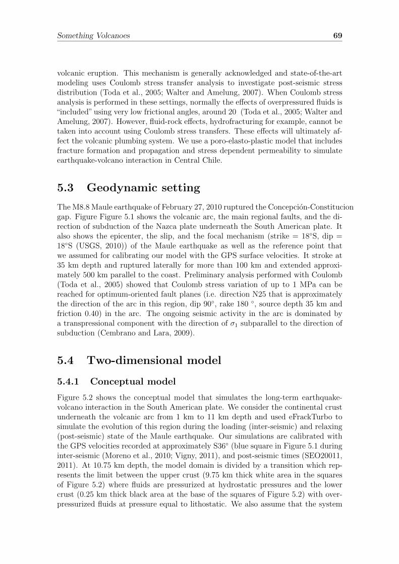
Something Volcanoes 69
volcanic eruption. This mechanism is generally acknowledged and state-of-the-artmodeling uses Coulomb stress transfer analysis to investigate post-seismic stressdistribution (Toda et al., 2005; Walter and Amelung, 2007). When Coulomb stressanalysis is performed in these settings, normally the effects of overpressured fluids is“included” using very low frictional angles, around 20 (Toda et al., 2005; Walter andAmelung, 2007). However, fluid-rock effects, hydrofracturing for example, cannot betaken into account using Coulomb stress transfers. These effects will ultimately af-fect the volcanic plumbing system. We use a poro-elasto-plastic model that includesfracture formation and propagation and stress dependent permeability to simulateearthquake-volcano interaction in Central Chile.
5.3 Geodynamic setting
The M8.8 Maule earthquake of February 27, 2010 ruptured the Concepcion-Constituciongap. Figure Figure 5.1 shows the volcanic arc, the main regional faults, and the di-rection of subduction of the Nazca plate underneath the South American plate. Italso shows the epicenter, the slip, and the focal mechanism (strike = 18S, dip =18S (USGS, 2010)) of the Maule earthquake as well as the reference point thatwe assumed for calibrating our model with the GPS surface velocities. It stroke at35 km depth and ruptured laterally for more than 100 km and extended approxi-mately 500 km parallel to the coast. Preliminary analysis performed with Coulomb(Toda et al., 2005) showed that Coulomb stress variation of up to 1 MPa can bereached for optimum-oriented fault planes (i.e. direction N25 that is approximatelythe direction of the arc in this region, dip 90, rake 180 , source depth 35 km andfriction 0.40) in the arc. The ongoing seismic activity in the arc is dominated bya transpressional component with the direction of σ1 subparallel to the direction ofsubduction (Cembrano and Lara, 2009).
5.4 Two-dimensional model
5.4.1 Conceptual model
Figure 5.2 shows the conceptual model that simulates the long-term earthquake-volcano interaction in the South American plate. We consider the continental crustunderneath the volcanic arc from 1 km to 11 km depth and used eFrackTurbo tosimulate the evolution of this region during the loading (inter-seismic) and relaxing(post-seismic) state of the Maule earthquake. Our simulations are calibrated withthe GPS velocities recorded at approximately S36 (blue square in Figure 5.1 duringinter-seismic (Moreno et al., 2010; Vigny, 2011), and post-seismic times (SEO20011,2011). At 10.75 km depth, the model domain is divided by a transition which rep-resents the limit between the upper crust (9.75 km thick white area in the squaresof Figure 5.2) where fluids are pressurized at hydrostatic pressures and the lowercrust (0.25 km thick black area at the base of the squares of Figure 5.2) with over-pressurized fluids at pressure equal to lithostatic. We also assume that the system
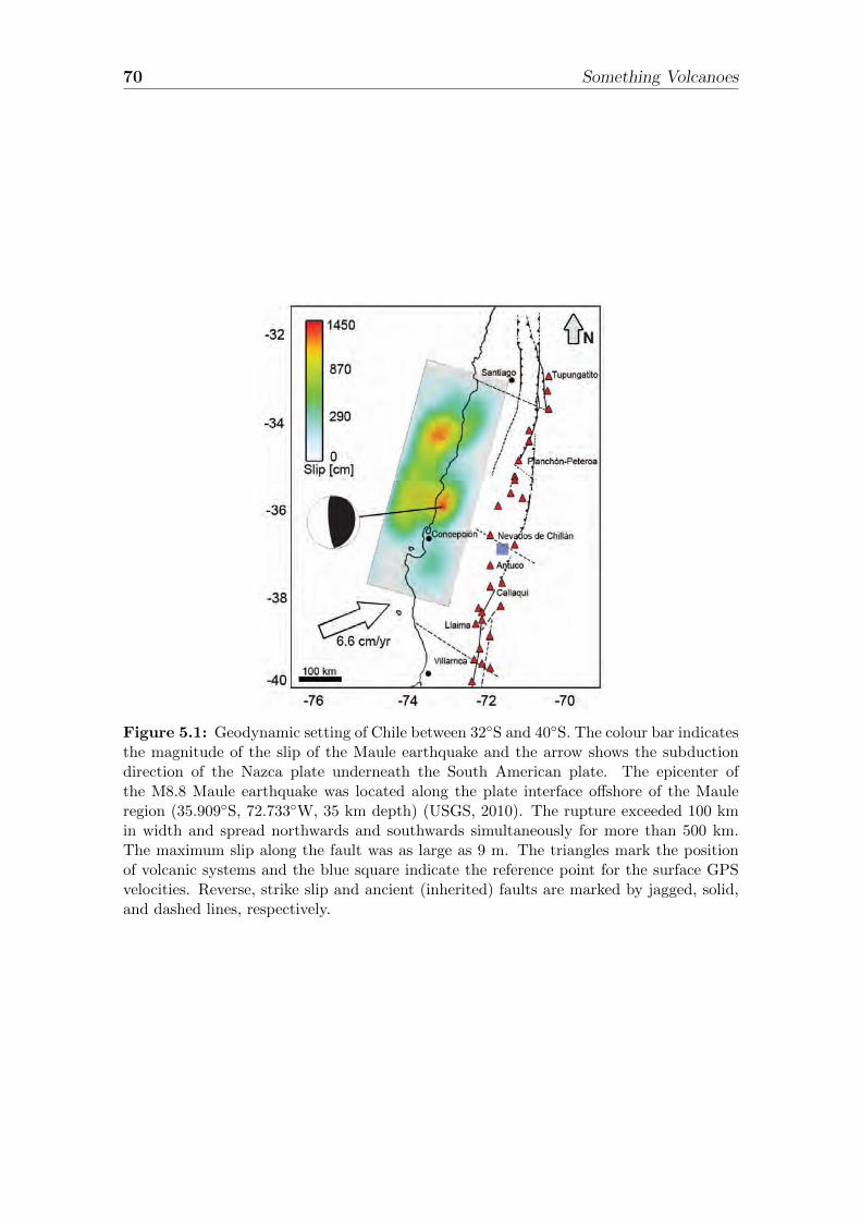
70 Something Volcanoes
Figure 5.1: Geodynamic setting of Chile between 32S and 40S. The colour bar indicatesthe magnitude of the slip of the Maule earthquake and the arrow shows the subductiondirection of the Nazca plate underneath the South American plate. The epicenter ofthe M8.8 Maule earthquake was located along the plate interface offshore of the Mauleregion (35.909S, 72.733W, 35 km depth) (USGS, 2010). The rupture exceeded 100 kmin width and spread northwards and southwards simultaneously for more than 500 km.The maximum slip along the fault was as large as 9 m. The triangles mark the positionof volcanic systems and the blue square indicate the reference point for the surface GPSvelocities. Reverse, strike slip and ancient (inherited) faults are marked by jagged, solid,and dashed lines, respectively.
Something Volcanoes 71
is compressional with σ1 horizontal and σ3 is given by the overburden.
Figure 5.2 illustrates the conceptual model of this study. The right column shows thegeodynamic state of the subduction zone and the left one shows the variation of thefar field stress states during the model. In particular, Figures 5.2a and 5.2b refer tothe inter-seismic state during which the system is in compression and the subductionis locked. This convergent setting is simulated to reproduce the approximately 175years that separate two different megathrust earthquakes. At this time, the GPSsurface velocities in the arc point Westwards and are approximately 1.125 cm yr−1
(Moreno et al., 2010). As the subduction goes on, σ1 can locally increase leading torock fracturing and fault failure (Figure 5.2b). Figure 5.2c shows the co-seismic stateduring which the Nazca plate suddenly slides underneath the South American plate.The maximum horizontal displacements recorded at the time of the earthquakenearby Concepcion is 4.7 m while in the arc it reached ∼50 cm (Vigny, 2011). Thistranslates to a sudden reduction of σ1 and to a general relaxation of the system5.2e. This volumetric expansion in the upper lithosphere underneath the volcanicarc that leads to a permeability increase and fracture uncloging or creation whichultimately facilitates the upwelling of deep fluids. Upwelling of fluids will increasethe fluid pressure at depth, reducing the normal effective stress required to failurethen promoting further failure, 5.2f.
5.4.2 Numerical model
We use a new GPU based software named eFrackTurbo. eFrackTurbo is a poro-elasto-plastic simulator for lithostatic models that includes nonlinear stress depen-dent permeability and is specially designed to allow creation of fractures and tofollow their evolution. eFrackTurbo solves the elastodynamics equations in theirvelocity-stress representation coupled with a nonlinear diffusion equation for thepore fluid pressure using explicit finite difference methods. It make use of the GPUparallel architecture to do high resolution computing in a very fast and efficient way.In our particular case, the model domain of 10×10 km is subdivided in a grid of300×300 elements given a resolution of 33 meters for each finite difference cell.
We model the continental crust below the volcanic arc as a heterogeneous fracturedrock. heterogeneities are introduced in the inital values of the frictional angle usingvalues normally distributed around 35 and in the cohesion taking random valuesaround 10 MPa. The elastic parameters are allow to change due to saturation orfracturing. In order to simulate strain weakening, the cohesion of the fractures isset to zero. The elastic properties, bulk modulus and Poisson radius evolve betweenthe prescribed values for the drained and undrained cases. Here the drained valuesrefers hydrostatic pore fluid pressure. For the bulk modulus we use Kd= 35 GPa andKu=41 for the drained and undrained rock and Poisson’s ratio νd=0.3 and νu=0.27.Crust density is 2700 kg m−3. The value of porosity was 1% for undrained rock and10% for undrained. The fluid pressure equation is similar to (Miller et al., 2004)(see appendix). The values of the intrinsic permeability, permeability at zero normalstress, are set to κdo = 10−19 m2 for the drained rock, κuo = 10−18 m2 for undrained
72 Something Volcanoes
Figure 5.2: Conceptual model (not to scale) of the simulation cycle. First, second, andthird row show the inter-seismic, co-seismic, and post-seismic state, respectively, undergoneby the upper crust of the South American plate over approximately two centuries. Thesquares in the left column represent the region of continental crust simulated in this study.Kv indicates the increase or decrease of permeability throughout the simulations. Thevertical line of circles indicates that the right boundary is fixed while the left black arrowson the left boundary indicate whether the system is in compression or extension. Thelength of the arrow is proportional to the GPS surface velocities.
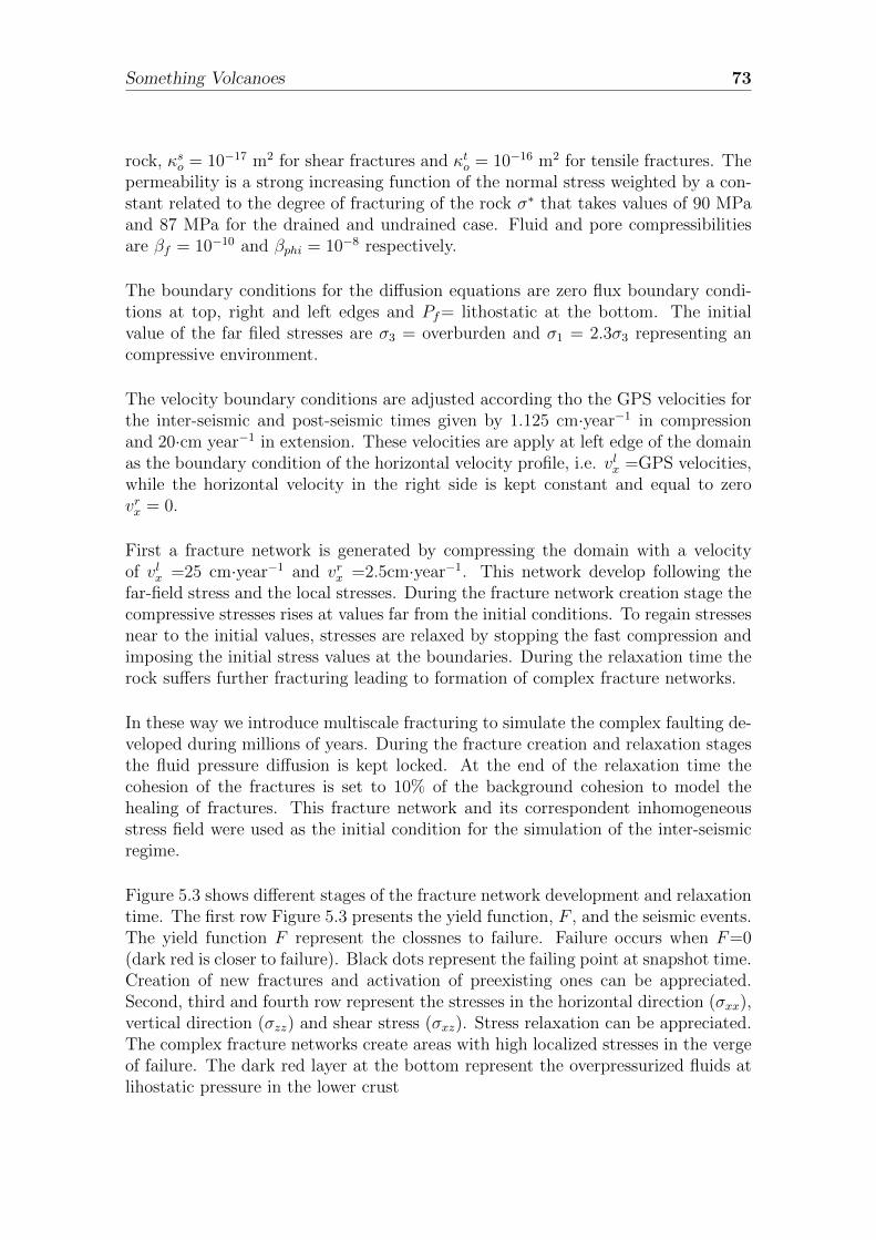
Something Volcanoes 73
rock, κso = 10−17 m2 for shear fractures and κto = 10−16 m2 for tensile fractures. Thepermeability is a strong increasing function of the normal stress weighted by a con-stant related to the degree of fracturing of the rock σ∗ that takes values of 90 MPaand 87 MPa for the drained and undrained case. Fluid and pore compressibilitiesare βf = 10−10 and βphi = 10−8 respectively.
The boundary conditions for the diffusion equations are zero flux boundary condi-tions at top, right and left edges and Pf= lithostatic at the bottom. The initialvalue of the far filed stresses are σ3 = overburden and σ1 = 2.3σ3 representing ancompressive environment.
The velocity boundary conditions are adjusted according tho the GPS velocities forthe inter-seismic and post-seismic times given by 1.125 cm·year−1 in compressionand 20·cm year−1 in extension. These velocities are apply at left edge of the domainas the boundary condition of the horizontal velocity profile, i.e. vlx =GPS velocities,while the horizontal velocity in the right side is kept constant and equal to zerovrx = 0.
First a fracture network is generated by compressing the domain with a velocityof vlx =25 cm·year−1 and vrx =2.5cm·year−1. This network develop following thefar-field stress and the local stresses. During the fracture network creation stage thecompressive stresses rises at values far from the initial conditions. To regain stressesnear to the initial values, stresses are relaxed by stopping the fast compression andimposing the initial stress values at the boundaries. During the relaxation time therock suffers further fracturing leading to formation of complex fracture networks.
In these way we introduce multiscale fracturing to simulate the complex faulting de-veloped during millions of years. During the fracture creation and relaxation stagesthe fluid pressure diffusion is kept locked. At the end of the relaxation time thecohesion of the fractures is set to 10% of the background cohesion to model thehealing of fractures. This fracture network and its correspondent inhomogeneousstress field were used as the initial condition for the simulation of the inter-seismicregime.
Figure 5.3 shows different stages of the fracture network development and relaxationtime. The first row Figure 5.3 presents the yield function, F , and the seismic events.The yield function F represent the clossnes to failure. Failure occurs when F=0(dark red is closer to failure). Black dots represent the failing point at snapshot time.Creation of new fractures and activation of preexisting ones can be appreciated.Second, third and fourth row represent the stresses in the horizontal direction (σxx),vertical direction (σzz) and shear stress (σxz). Stress relaxation can be appreciated.The complex fracture networks create areas with high localized stresses in the vergeof failure. The dark red layer at the bottom represent the overpressurized fluids atlihostatic pressure in the lower crust
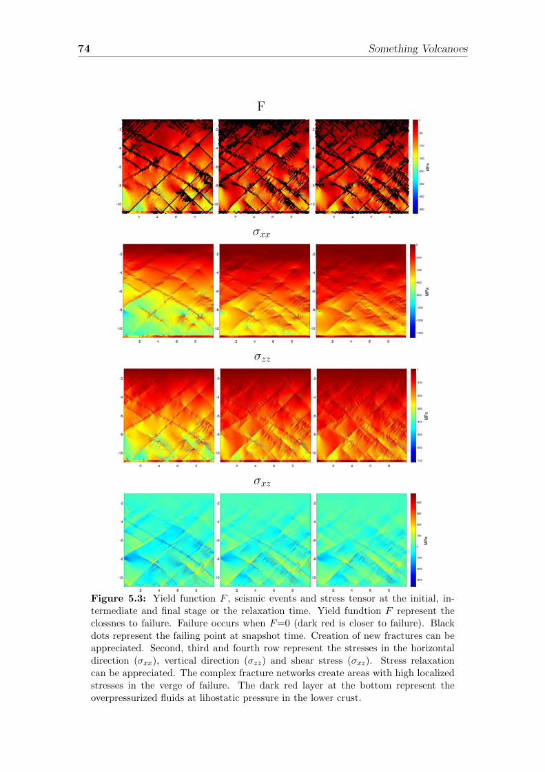
74 Something Volcanoes
F
σxx
σzz
σxz
Figure 5.3: Yield function F , seismic events and stress tensor at the initial, in-termediate and final stage or the relaxation time. Yield fundtion F represent theclossnes to failure. Failure occurs when F=0 (dark red is closer to failure). Blackdots represent the failing point at snapshot time. Creation of new fractures can beappreciated. Second, third and fourth row represent the stresses in the horizontaldirection (σxx), vertical direction (σzz) and shear stress (σxz). Stress relaxationcan be appreciated. The complex fracture networks create areas with high localizedstresses in the verge of failure. The dark red layer at the bottom represent theoverpressurized fluids at lihostatic pressure in the lower crust.
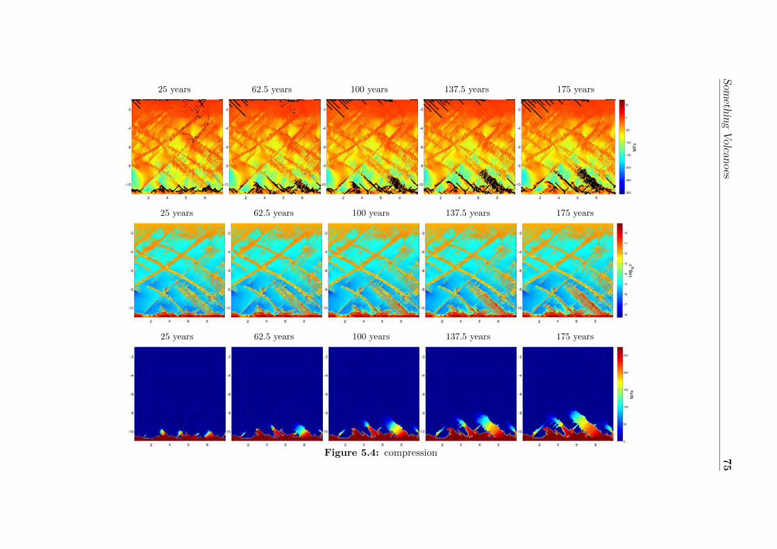
Som
ethingVolcan
oes
75
25 years 62.5 years 100 years 137.5 years 175 years
25 years 62.5 years 100 years 137.5 years 175 years
25 years 62.5 years 100 years 137.5 years 175 years
Figure 5.4: compression
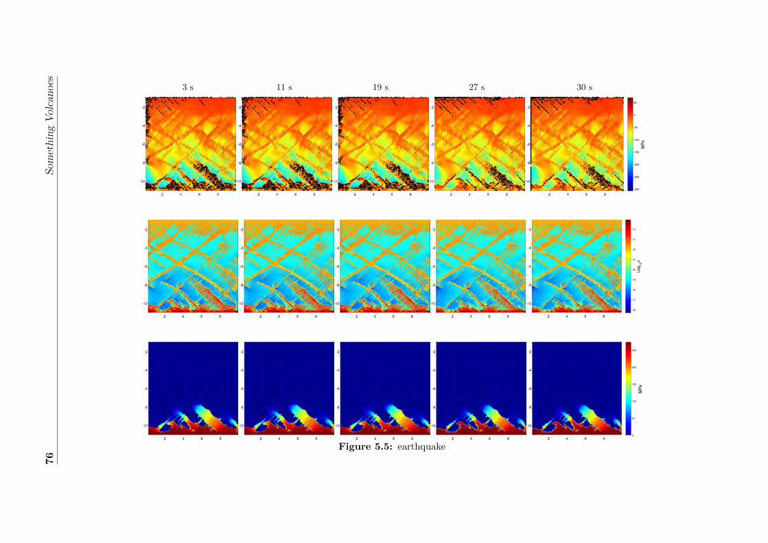
76
Som
ethingVolcanoes
3 s 11 s 19 s 27 s 30 s
Figure 5.5: earthquake
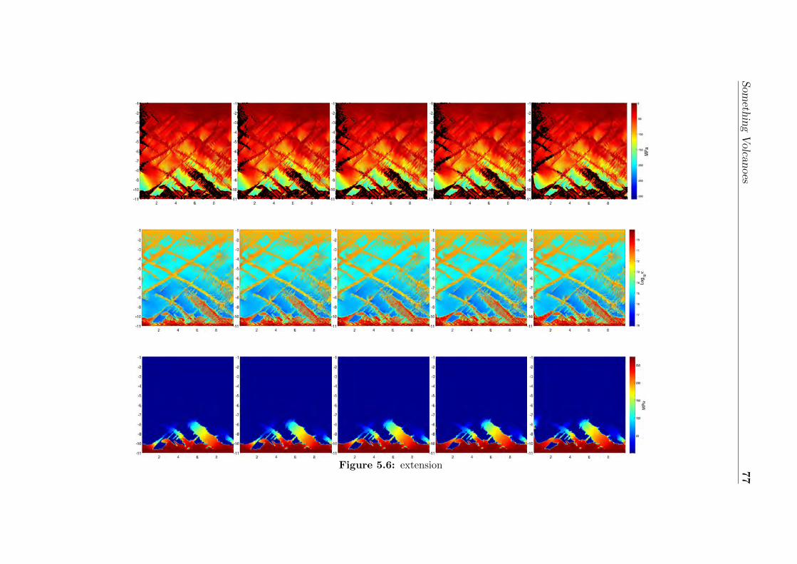
Som
ethingVolcan
oes
77
Figure 5.6: extension
78 Something Volcanoes
5.5 Conclusions
Earthquake volcano interactions in the central part of Chile were modeled using aporo-elasto-plastic model with stress dependent permeability for the pore fluid pres-sure difusion equation. The results shows that post seismic expasion enhance fluidmobilization through fracture channels. The reduction in the normal stress leadsto a increase in the permeability of the fractures. Fluid promotes more fracturingallong the low paths which induce more fluid mnobilization. The sudden increase ofthe permeability coupled to further fracturing results in very fast upwards flow.
Future developments of this model will include the simulation of the co-seismicregime and the effects of seismic waves and dynamic stresses. These effects of theslipping are significant because fracture aperture and faster fracture grow are realtedto it.
5.6 Acknowledgments
I thank Dr. Matteo Lupi for it help in discussion and geology remarks used in thepresent work. We thank the German Research Foundation, Deutsche Forschungsge-meinschaft (DFG) for the financial support through the project no. MI 1237/2-1.

Part III
CONCLUDING REMARKS
79


Chapter 6
Concluding Remarks and FutureWork
Many different phenomena of lithospheric geodynamics can be described by fluid-rock interactions. These interactions are complex across multiple scales in time andspace, and powerful numerical techniques must be developed to capture this multi-scaled problem. However, these techniques demand equally expensive computationalresources, limiting in many cases their widespread application. CPU clusters havebeen the main tool to deal with high resolution simulations introducing anotherlimiting factor as the high level of expertise required to program these complex nu-merical models in a physically correct way on this architecture. Despite the vastimprovement of CPU technology, most of the current numerical models are stillsimulated in relatively low resolution. From the point of view of CPU computing,there has not been a significant advancement in routine scientific modeling in thelast 20 years. Low resolution models, even when they encompass sufficient physics,may lead to inaccurate results because of the numerical limitations. Limited resolu-tion of numerical models have similarly limited application to real world problems,and high resolution computing is regarded by many as merely and optimization issue.
I have presented simulations of hydro-mechanically coupled systems with very dif-ferent time and space scales from numerical simulation of laboratory experiments,applications to geothermal systems and for larger scales models of fluid mobilizationrelated to aftershocks triggering, with time scales ranging from some minutes tomonths and years. The multiscality problem can be handle at high resolutions in anefficient way. For the laboratory experiments simulation length scales in the rangeof tenths of millimeters were achieved while in the fluid mobilization experiments,where the total scales is in the range of kilometers, resolutions of meters were pos-sible. The range of possible length scales is up to three orders of magnitude. Intime scales a difference up to six orders of magnitude is possible. This large rangeof resolutions allows to develop software tools that have a real applicability for realworld problems and it allows to study very complex dynamics in details.
The numerical codes were benchmarked comparing the results of shear fracture for-
81
82 Concluding Remarks
mation experiments with other elastoplastic codes. The Method of ManufacturedSolutions (MMS) was used to benchmark the non-linear diffusion model. Solutionsfor the elasto-plastic part of the code shows excellent agreement with other reports(Poliakov et al., 1994; Kaus, 2010; Popov and Sobolev, 2008; Hansen, 2003). UsingMMS for the nonlinear diffusion part the GPU code gives exactly the same solutionas the CPU code. The results presented in this thesis are the first implementationof Poro-elasto-plastic media in GPU and, to the best of our knowledge, this is oneof the few numerical codes that can follow the creation and evolution of fracturenetworks in geo-materials. Due to the increment in speed and resolution of GPUbased codes is possible to model a manifold of systems with the same code withoutany major change.
The baseline code presented here sets the basis for many future improvements anddevelopments, including its extension the 3D. In terms of physics, an improvedtreatment of porosity creation and destruction, and changes in hydraulic and elasticproperties is to be explored. Damage effects on elastic properties have so far beenignored, while thermo-elasticity should be introduced to extend this model to a morerealistic simulator of geo-thermal systems.
A future and systematic and focused study should be performed to investigate theoptimal approach to handling the complex properties of permeability in relation toporosity, strain, frictional or tensional failure, or how permeability is influenced byeffective normals stresses or crack aperture. The results of these studies will establishthe optimal algorithmic approach for computational efficiency and physical accuracy.
The source term in the nonlinear pore fluid diffusion equation might be importantfor large earthquake modeling. Heating of the fault plane may induce decarboniza-tion reactions in the fault and trapping high pressure fluids that promote additionalslip (Madariaga, 2007; Paola et al., 2011). In geothermal and volcanic systems theheat effects are essential. To model this is necessary to introduce thermal effectsusing the advection diffusion equation of heat. The effect of heat on the fluid andon the rock will be introduced in future versions of our code. A full thermo-poro-elasto-plastic GPU model is envisioned.
Another necessary improvement is the 3D implementation of the code. For realapplications in EGS or fracking the 3D modeling of the fracture networks is very ap-pealing. Developing a 3D code at the high resolution desired will likely incorporatea GPU cluster in the future, and we are currently working making developmentsin this direction. The simulation of the Basel geothermal systems presented in thiswork was computed on a single GPU card. However, we present results with a veryhigh resolution, of just 25cm per cell, and a large simulation domain of 500 m, i.e.a grid of 2000×2000. The utilization of GPU cluster to compute a the 3D modelpromises very high resolutions too.
Further, calibration of the model and quantitative comparisons to experiments is
Concluding Remarks 83
necessary.Visualization of high resolution results, in particular for the 3D implementation, willrequire a graphical interface. Part of our future work is to complement this codewith pre-processing and a post-processing tools. The goal in to have a fast and easyto use software for thermo-hydro-mechanical modeling.
High resolution modeling opens the possibility of following the evolution of the cou-pled systems and accurate modeling can be performed. Faster numerical modelsthat include all of the underlying physics has always been the goal in geodynamicalnumerical model. GPU technology allows faster simulations at higher resolution,while not sacrificing the physical processes being simulated. The work presentedhere is another step in the development of such numerical codes.
My personal view is that the future in scientific numerical modeling, irrespective ofthe area under study, will require faster and high resolution codes, where resolutionand speed are not just optimization issues but limiting factors in unveiling the un-derlying physics. GPU technology might provide a solution for this problem.

84 Concluding Remarks

Appendix
85

Geology
doi: 10.1130/G31457.1 2010;38;995-998Geology
Toshiko Terakawa, Anna Zoporowski, Boris Galvan and Stephen A. Miller earthquake focal mechanismsHigh-pressure fluid at hypocentral depths in the L'Aquila region inferred from
Email alerting servicesarticles cite this article
to receive free e-mail alerts when newwww.gsapubs.org/cgi/alertsclick
Subscribe to subscribe to Geologywww.gsapubs.org/subscriptions/click
Permission request to contact GSAhttp://www.geosociety.org/pubs/copyrt.htm#gsaclick
official positions of the Society.citizenship, gender, religion, or political viewpoint. Opinions presented in this publication do not reflectpresentation of diverse opinions and positions by scientists worldwide, regardless of their race, includes a reference to the article's full citation. GSA provides this and other forums for thethe abstracts only of their articles on their own or their organization's Web site providing the posting to further education and science. This file may not be posted to any Web site, but authors may postworks and to make unlimited copies of items in GSA's journals for noncommercial use in classrooms requests to GSA, to use a single figure, a single table, and/or a brief paragraph of text in subsequenttheir employment. Individual scientists are hereby granted permission, without fees or further Copyright not claimed on content prepared wholly by U.S. government employees within scope of
Notes
© 2010 Geological Society of America
on February 3, 2012geology.gsapubs.orgDownloaded from
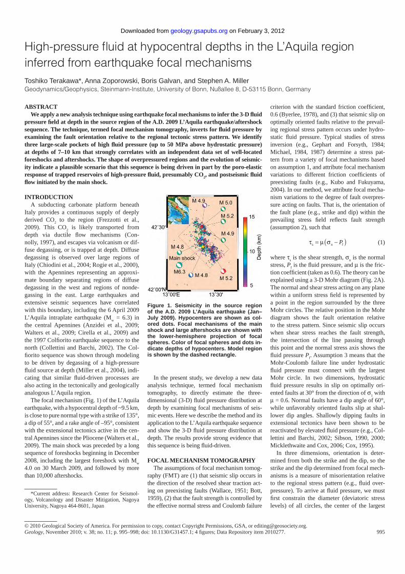
GEOLOGY, November 2010 995
INTRODUCTIONA subducting carbonate platform beneath
Italy provides a continuous supply of deeply derived CO2 to the region (Frezzotti et al., 2009). This CO2 is likely transported from depth via ductile fl ow mechanisms (Con-nolly, 1997), and escapes via volcanism or dif-fuse degassing, or is trapped at depth. Diffuse degassing is observed over large regions of Italy (Chiodini et al., 2004; Rogie et al., 2000), with the Apennines representing an approxi-mate boundary separating regions of diffuse degassing in the west and regions of nonde-gassing in the east. Large earthquakes and extensive seismic sequences have correlated with this boundary, including the 6 April 2009 L’Aquila intraplate earthquake (Mw = 6.3) in the central Apennines (Anzidei et al., 2009; Walters et al., 2009; Cirella et al., 2009) and the 1997 Colfi orito earthquake sequence to the north (Collettini and Barchi, 2002). The Col-fi orito sequence was shown through modeling to be driven by degassing of a high-pressure fl uid source at depth (Miller et al., 2004), indi-cating that similar fl uid-driven processes are also acting in the tectonically and geologically analogous L’Aquila region.
The focal mechanism (Fig. 1) of the L’Aquila earthquake, with a hypocentral depth of ~9.5 km, is close to pure normal type with a strike of 135°, a dip of 55°, and a rake angle of –95°, consistent with the extensional tectonics active in the cen-tral Apennines since the Pliocene (Walters et al., 2009). The main shock was preceded by a long sequence of foreshocks beginning in December 2008, including the largest foreshock with Mw 4.0 on 30 March 2009, and followed by more than 10,000 aftershocks.
In the present study, we develop a new data analysis technique, termed focal mechanism tomography, to directly estimate the three-dimensional (3-D) fl uid pressure distribution at depth by examining focal mechanisms of seis-mic events. Here we describe the method and its application to the L’Aquila earthquake sequence and show the 3-D fl uid pressure distribution at depth. The results provide strong evidence that this sequence is being fl uid-driven.
FOCAL MECHANISM TOMOGRAPHYThe assumptions of focal mechanism tomog-
raphy (FMT) are (1) that seismic slip occurs in the direction of the resolved shear traction act-ing on preexisting faults (Wallace, 1951; Bott, 1959), (2) that the fault strength is controlled by the effective normal stress and Coulomb failure
criterion with the standard friction coeffi cient, 0.6 (Byerlee, 1978), and (3) that seismic slip on optimally oriented faults relative to the prevail-ing regional stress pattern occurs under hydro-static fl uid pressure. Typical studies of stress inversion (e.g., Gephart and Forsyth, 1984; Michael, 1984, 1987) determine a stress pat-tern from a variety of focal mechanisms based on assumption 1, and attribute focal mechanism variations to different friction coeffi cients of preexisting faults (e.g., Kubo and Fukuyama, 2004). In our method, we attribute focal mecha-nism variations to the degree of fault overpres-sure acting on faults. That is, the orientation of the fault plane (e.g., strike and dip) within the prevailing stress fi eld refl ects fault strength (assumption 2), such that
τ μ σs n f= −( )P (1)
where τs is the shear strength, σn is the normal stress, Pf is the fl uid pressure, and μ is the fric-tion coeffi cient (taken as 0.6). The theory can be explained using a 3-D Mohr diagram (Fig. 2A). The normal and shear stress acting on any plane within a uniform stress fi eld is represented by a point in the region surrounded by the three Mohr circles. The relative position in the Mohr diagram shows the fault orientation relative to the stress pattern. Since seismic slip occurs when shear stress reaches the fault strength, the intersection of the line passing through this point and the normal stress axis shows the fl uid pressure Pf. Assumption 3 means that the Mohr-Coulomb failure line under hydrostatic fl uid pressure must connect with the largest Mohr circle. In two dimensions, hydrostatic fl uid pressure results in slip on optimally ori-ented faults at 30° from the direction of σ1 with μ = 0.6. Normal faults have a dip angle of 60°, while unfavorably oriented faults slip at shal-lower dip angles. Shallowly dipping faults in extensional tectonics have been shown to be reactivated by elevated fl uid pressure (e.g., Col-lettini and Barchi, 2002; Sibson, 1990, 2000; Micklethwaite and Cox, 2006; Cox, 1995).
In three dimensions, orientation is deter-mined from both the strike and the dip, so the strike and the dip determined from focal mech-anisms is a measure of misorientation relative to the regional stress pattern (e.g., fl uid over-pressure). To arrive at fl uid pressure, we must fi rst constrain the diameter (deviatoric stress levels) of all circles, the center of the largest
Geology, November 2010; v. 38; no. 11; p. 995–998; doi: 10.1130/G31457.1; 4 fi gures; Data Repository item 2010277.© 2010 Geological Society of America. For permission to copy, contact Copyright Permissions, GSA, or [email protected].
*Current address: Research Center for Seismol-ogy, Volcanology and Disaster Mitigation, Nagoya University, Nagoya 464-8601, Japan
High-pressure fl uid at hypocentral depths in the L’Aquila region inferred from earthquake focal mechanismsToshiko Terakawa*, Anna Zoporowski, Boris Galvan, and Stephen A. MillerGeodynamics/Geophysics, Steinmann-Institute, University of Bonn, Nußallee 8, D-53115 Bonn, Germany
ABSTRACTWe apply a new analysis technique using earthquake focal mechanisms to infer the 3-D fl uid
pressure fi eld at depth in the source region of the A.D. 2009 L’Aquila earthquake/aftershock sequence. The technique, termed focal mechanism tomography, inverts for fl uid pressure by examining the fault orientation relative to the regional tectonic stress pattern. We identify three large-scale pockets of high fl uid pressure (up to 50 MPa above hydrostatic pressure) at depths of 7–10 km that strongly correlates with an independent data set of well-located foreshocks and aftershocks. The shape of overpressured regions and the evolution of seismic-ity indicate a plausible scenario that this sequence is being driven in part by the poro-elastic response of trapped reservoirs of high-pressure fl uid, presumably CO2, and postseismic fl uid fl ow initiated by the main shock.
Figure 1. Seismicity in the source region of the A.D. 2009 L’Aquila earthquake (Jan–July 2009). Hypocenters are shown as col-ored dots. Focal mechanisms of the main shock and large aftershocks are shown with the lower-hemisphere projection of focal spheres. Color of focal spheres and dots in-dicate depths of hypocenters. Model region is shown by the dashed rectangle.
on February 3, 2012geology.gsapubs.orgDownloaded from
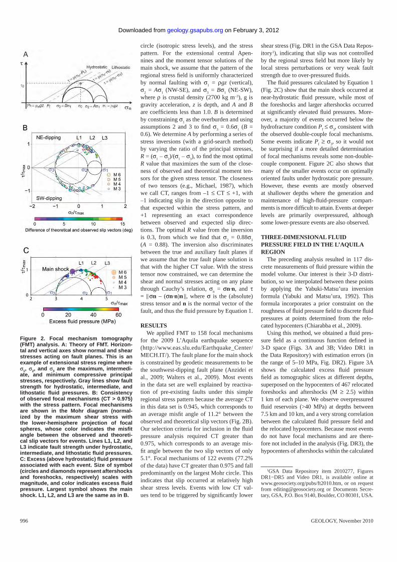
996 GEOLOGY, November 2010
circle (isotropic stress levels), and the stress pattern. For the extensional central Apen-nines and the moment tensor solutions of the main shock, we assume that the pattern of the regional stress fi eld is uniformly characterized by normal faulting with σ1 = ρgz (vertical), σ2 = Aσ1 (NW-SE), and σ3 = Bσ1 (NE-SW), where ρ is crustal density (2700 kg m–3), g is gravity acceleration, z is depth, and A and B are coeffi cients less than 1.0. B is determined by constraining σ1 as the overburden and using assumptions 2 and 3 to fi nd σ3 = 0.6σ1 (B = 0.6). We determine A by performing a series of stress inversions (with a grid-search method) by varying the ratio of the principal stresses, R = (σ1 – σ2)/(σ1 – σ3), to fi nd the most optimal R value that maximizes the sum of the close-ness of observed and theoretical moment ten-sors for the given stress tensor. The closeness of two tensors (e.g., Michael, 1987), which we call CT, ranges from –1 ≤ CT ≤ +1, with –1 indicating slip in the direction opposite to that expected within the stress pattern, and +1 representing an exact correspondence between observed and expected slip direc-tions. The optimal R value from the inversion is 0.3, from which we fi nd that σ2 = 0.88σ1 (A = 0.88). The inversion also discriminates between the true and auxiliary fault planes if we assume that the true fault plane solution is that with the higher CT value. With the stress tensor now constrained, we can determine the shear and normal stresses acting on any plane through Cauchy’s relation, σn = σn·n, and τ = σn – (σn·n)n , where σ is the (absolute) stress tensor and n is the normal vector of the fault, and thus the fl uid pressure by Equation 1.
RESULTSWe applied FMT to 158 focal mechanisms
for the 2009 L’Aquila earthquake sequence (http://www.eas.slu.edu/Earthquake_Center/MECH.IT/). The fault plane for the main shock is constrained by geodetic measurements to be the southwest-dipping fault plane (Anzidei et al., 2009; Walters et al., 2009). Most events in the data set are well explained by reactiva-tion of pre-existing faults under this simple regional stress pattern because the average CT in this data set is 0.945, which corresponds to an average misfi t angle of 11.2° between the observed and theoretical slip vectors (Fig. 2B). Our selection criteria for inclusion in the fl uid pressure analysis required CT greater than 0.975, which corresponds to an average mis-fi t angle between the two slip vectors of only 5.1°. Focal mechanisms of 122 events (77.2% of the data) have CT greater than 0.975 and fall predominantly on the largest Mohr circle. This indicates that slip occurred at relatively high shear stress levels. Events with low CT val-ues tend to be triggered by signifi cantly lower
shear stress (Fig. DR1 in the GSA Data Repos-itory1), indicating that slip was not controlled by the regional stress fi eld but more likely by local stress perturbations or very weak fault strength due to over-pressured fl uids.
The fl uid pressures calculated by Equation 1 (Fig. 2C) show that the main shock occurred at near-hydrostatic fl uid pressure, while most of the foreshocks and larger aftershocks occurred at signifi cantly elevated fl uid pressures. More-over, a majority of events occurred below the hydrofracture condition Pf ≤ σ3, consistent with the observed double-couple focal mechanisms. Some events indicate Pf ≥ σ3, so it would not be surprising if a more detailed determination of focal mechanisms reveals some non-double-couple component. Figure 2C also shows that many of the smaller events occur on optimally oriented faults under hydrostatic pore pressure. However, these events are mostly observed at shallower depths where the generation and maintenance of high-fl uid-pressure compart-ments is more diffi cult to attain. Events at deeper levels are primarily overpressured, although some lower-pressure events are also observed.
THREE-DIMENSIONAL FLUID PRESSURE FIELD IN THE L’AQUILA REGION
The preceding analysis resulted in 117 dis-crete measurements of fl uid pressure within the model volume. Our interest is their 3-D distri-bution, so we interpolated between these points by applying the Yabuki-Matsu’ura inversion formula (Yabuki and Matsu’ura, 1992). This formula incorporates a prior constraint on the roughness of fl uid pressure fi eld to discrete fl uid pressures at points determined from the relo-cated hypocenters (Chiarabba et al., 2009).
Using this method, we obtained a fl uid pres-sure fi eld as a continuous function defi ned in 3-D space (Figs. 3A and 3B; Video DR1 in the Data Repository) with estimation errors (in the range of 5–10 MPa, Fig. DR2). Figure 3A shows the calculated excess fl uid pressure fi eld as tomographic slices at different depths, superposed on the hypocenters of 467 relocated foreshocks and aftershocks (M ≥ 2.5) within 1 km of each plane. We observe overpressured fl uid reservoirs (>40 MPa) at depths between 7.5 km and 10 km, and a very strong correlation between the calculated fl uid pressure fi eld and the relocated hypocenters. Because most events do not have focal mechanisms and are there-fore not included in the analysis (Fig. DR3), the hypocenters of aftershocks within the calculated
1GSA Data Repository item 2010277, Figures DR1−DR5 and Video DR1, is available online at www.geosociety.org/pubs/ft2010.htm, or on request from [email protected] or Documents Secre-tary, GSA, P.O. Box 9140, Boulder, CO 80301, USA.
Figure 2. Focal mechanism tomography (FMT) analysis. A: Theory of FMT. Horizon-tal and vertical axes show normal and shear stresses acting on fault planes. This is an example of extensional stress regime where σ1, σ2, and σ3 are the maximum, intermedi-ate, and minimum compressive principal stresses, respectively. Gray lines show fault strength for hydrostatic, intermediate, and lithostatic fl uid pressures. B: Consistency of observed focal mechanisms (CT > 0.975) with the stress pattern. Focal mechanisms are shown in the Mohr diagram (normal-ized by the maximum shear stress with the lower-hemisphere projection of focal spheres, whose color indicates the misfi t angle between the observed and theoreti-cal slip vectors for events. Lines L1, L2, and L3 indicate fault strength under hydrostatic, intermediate, and lithostatic fl uid pressures. C: Excess (above hydrostatic) fl uid pressure associated with each event. Size of symbol (circles and diamonds represent aftershocks and foreshocks, respectively) scales with magnitude, and color indicates excess fl uid pressure. Largest symbol shows the main shock. L1, L2, and L3 are the same as in B.
on February 3, 2012geology.gsapubs.orgDownloaded from
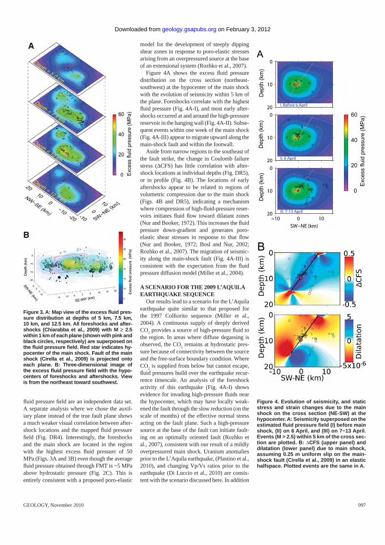
GEOLOGY, November 2010 997
fl uid pressure fi eld are an independent data set. A separate analysis where we chose the auxil-iary plane instead of the true fault plane shows a much weaker visual correlation between after-shock locations and the mapped fl uid pressure fi eld (Fig. DR4). Interestingly, the foreshocks and the main shock are located in the region with the highest excess fl uid pressure of 50 MPa (Figs. 3A and 3B) even though the average fl uid pressure obtained through FMT is ~5 MPa above hydrostatic pressure (Fig. 2C). This is entirely consistent with a proposed poro-elastic
model for the development of steeply dipping shear zones in response to poro-elastic stresses arising from an overpressured source at the base of an extensional system (Rozhko et al., 2007).
Figure 4A shows the excess fl uid pressure distribution on the cross section (northeast-southwest) at the hypocenter of the main shock with the evolution of seismicity within 5 km of the plane. Foreshocks correlate with the highest fl uid pressure (Fig. 4A-I), and most early after-shocks occurred at and around the high-pressure reservoir in the hanging wall (Fig. 4A-II). Subse-quent events within one week of the main shock (Fig. 4A-III) appear to migrate upward along the main-shock fault and within the footwall.
Aside from narrow regions to the southeast of the fault strike, the change in Coulomb failure stress (ΔCFS) has little correlation with after-shock locations at individual depths (Fig. DR5), or in profi le (Fig. 4B). The locations of early aftershocks appear to be related to regions of volumetric compression due to the main shock (Figs. 4B and DR5), indicating a mechanism where compression of high-fl uid-pressure reser-voirs initiates fl uid fl ow toward dilatant zones (Nur and Booker, 1972). This increases the fl uid pressure down-gradient and generates poro-elastic shear stresses in response to that fl ow (Nur and Booker, 1972; Bosl and Nur, 2002; Rozhko et al., 2007). The migration of seismic-ity along the main-shock fault (Fig. 4A-III) is consistent with the expectation from the fl uid pressure diffusion model (Miller et al., 2004).
A SCENARIO FOR THE 2009 L’AQUILA EARTHQUAKE SEQUENCE
Our results lead to a scenario for the L’Aquila earthquake quite similar to that proposed for the 1997 Colfi orito sequence (Miller et al., 2004). A continuous supply of deeply derived CO2 provides a source of high-pressure fl uid to the region. In areas where diffuse degassing is observed, the CO2 remains at hydrostatic pres-sure because of connectivity between the source and the free-surface boundary condition. Where CO2 is supplied from below but cannot escape, fl uid pressures build over the earthquake recur-rence timescale. An analysis of the foreshock activity of this earthquake (Fig. 4A-I) shows evidence for invading high-pressure fl uids near the hypocenter, which may have locally weak-ened the fault through the slow reduction (on the scale of months) of the effective normal stress acting on the fault plane. Such a high-pressure source at the base of the fault can initiate fault-ing on an optimally oriented fault (Rozhko et al., 2007), consistent with our result of a mildly overpressured main shock. Uranium anomalies prior to the L’Aquila earthquake, (Plastino et al., 2010), and changing Vp/Vs ratios prior to the earthquake (Di Luccio et al., 2010) are consis-tent with the scenario discussed here. In addition
Figure 3. A: Map view of the excess fl uid pres-sure distribution at depths of 5 km, 7.5 km, 10 km, and 12.5 km. All foreshocks and after-shocks (Chiarabba et al., 2009) with M ≥ 2.5 within 1 km of each plane (shown with pink and black circles, respectively) are superposed on the fl uid pressure fi eld. Red star indicates hy-pocenter of the main shock. Fault of the main shock (Cirella et al., 2009) is projected onto each plane. B: Three-dimensional image of the excess fl uid pressure fi eld with the hypo-centers of foreshocks and aftershocks. View is from the northeast toward southwest.
Figure 4. Evolution of seismicity, and static stress and strain changes due to the main shock on the cross section (NE-SW) at the hypocenter. A: Seismicity superposed on the estimated fl uid pressure fi eld (I) before main shock, (II) on 6 April, and (III) on 7−13 April. Events (M > 2.5) within 5 km of the cross sec-tion are plotted. B: ΔCFS (upper panel) and dilatation (lower panel) due to main shock, assuming 0.25 m uniform slip on the main-shock fault (Cirella et al., 2009) in an elastic halfspace. Plotted events are the same in A.
on February 3, 2012geology.gsapubs.orgDownloaded from
998 GEOLOGY, November 2010
to other transient mechanisms such as dynamic triggering that are very effective in fl uid-rich environments (Hill et al., 1993), the main shock volumetrically compressed the surrounding overpressured poro-elastic medium, initiating fl uid fl ow. One possible explanation for the extensive aftershock activity is postseismic fl uid fl ow triggered by perturbing an extensive and overpressured reservoir at depth. Importantly, since the main shock and each aftershock also correspond to the creation of a fresh fracture (Miller and Nur, 2000), the network has evolv-ing hydraulic properties that signifi cantly infl u-ence fl uid fl ow and thus contribute to the com-plexity of this sequence.
This analysis provides important constraints on the shape and magnitude of the deep fl uid pressure fi eld, and therefore provides an impor-tant boundary condition for forward modeling and mechanistic hazard assessment. That both the Omori and Gutenberg-Richter laws are sat-isfi ed makes this sequence indistinguishable from other earthquake/aftershock sequences, suggesting that similar processes may be act-ing elsewhere.
ACKNOWLEDGMENTSWe thank Robert Herrmann for providing the fo-
cal mechanism data and Lauro Chiaraluce for discus-sions and for providing the relocated hypocenter data catalogue. This study was supported in part by DFG Project MI 1237/2-1.
REFERENCES CITEDAnzidei, M., Boschi, E., Cannelli, V., Devoti, R., Es-
posito, A., Galvani, A., Melini, D., Pietrantonio, G., Riguzzi, F., Sepe, V., and Serpelloni, E., 2009, Coseismic deformation of the destructive April 6, 2009 L’Aquila earthquake (central Italy) from GPS data: Geophysical Research Letters, v. 36, L17307, doi: 10.1029/2009GL039145.
Bosl, W.J., and Nur, A., 2002, Aftershocks and pore fl uid diffusion following the 1992 Landers earthquake: Journal of Geophysical Research (Solid Earth), v. 107, 2366, doi: 10.1029/2001JB000155.
Bott, M.H.P., 1959, The mechanics of oblique slip faulting: Geological Magazine, v. 96, p. 109–117, doi: 10.1017/S0016756800059987.
Byerlee, J., 1978, Friction of rocks: Pure and Applied Geophysics, v. 116, p. 615–626, doi: 10.1007/BF00876528.
Chiarabba, C., and 29 others, 2009, The 2009 L’Aquila (central Italy) Mw 6.3 earthquake: Main shock and aftershocks: Geophysical Re-search Letters, v. 36, L18308, doi: 10.1029/2009GL039627.
Chiodini, G., Cardellini, C., Amato, A., Boschi, E., Caliro, S., Frondini, F., and Ventura, G., 2004, Carbon dioxide Earth degassing and seismo-
genesis in central and southern Italy: Geo-physical Research Letters, v. 31, L07615, doi: 10.1029/2004GL019480.
Cirella, A., Piatanesi, A., Cocco, M., Tinti, E., Scog-namiglio, L., Michelini, A., Lomax, A., and Boschi, E., 2009, Rupture history of the 2009 L’Aquila (Italy) earthquake from non-linear joint inversion of strong motion and GPS data: Geophysical Research Letters, v. 36, L19304, doi: 10.1029/2009GL039795.
Collettini, C., and Barchi, M.R., 2002, A low-angle normal fault in the Umbria region (Central It-aly): A mechanical model for the related micro-seismicity: Tectonophysics, v. 359, p. 97–115, doi: 10.1016/S0040-1951(02)00441-9.
Connolly, J.A.D., 1997, Devolatilization-generated fl uid pressure and deformation-propagated fl uid fl ow during prograde regional metamor-phism: Journal of Geophysical Research (Solid Earth), v. 102, p. 18,149–18,173, doi: 10.1029/97JB00731.
Cox, S.F., 1995, Faulting processes at high fl uid pressures: An example of fault valve behav-ior from the Wattle Gully Fault, Victoria, Australia: Journal of Geophysical Research (Solid Earth), v. 100, p. 12,841–12,859, doi: 10.1029/95JB00915.
Di Luccio, F., Ventura, G., Di Giovambattista, R., Piscini, A. and Cinti, F.R., 2010, Normal faults and thrusts activated by deep fl uids: The 6 April 2009 Mw 6.3 L’Aquila earthquake, Central Italy: Journal of Geophysical Re-search, doi:10.1029/2009JB007190.
Frezzotti, M.L., Peccerillo, A., and Panza, G., 2009, Carbonate metasomatism and CO2 lithosphere-asthenosphere degassing beneath the Western Mediterranean: An integrated model aris-ing from petrological and geophysical data: Chemical Geology, v. 262, p. 108–120, doi: 10.1016/j.chemgeo.2009.02.015.
Gephart, J.W., and Forsyth, D.W., 1984, An im-proved method for determining the regional stress tensor using earthquake focal mecha-nism data: Application to the San Fernando earthquake sequence: Journal of Geophysical Research, v. 89, p. 9305–9320, doi: 10.1029/JB089iB11p09305.
Hill, D.P., and 30 others, 1993, Seismicity remotely triggered by the magnitude 7.3 Landers, Cali-fornia, earthquake: Science, v. 260, p. 1617–1623, doi: 10.1126/science.260.5114.1617.
Kubo, A., and Fukuyama, E., 2004, Stress fi elds and fault reactivation angles of the 2000 west-ern Tottori aftershocks and the 2001 northern Hyogo swarm in southwest Japan: Tectono-physics, v. 378, p. 223–239, doi: 10.1016/j.tecto.2003.09.009.
Michael, A.J., 1984, Determination of stress from slip data: Faults and folds: Journal of Geo-physical Research, v. 89, p. 1517–1526, doi: 10.1029/JB089iB13p11517.
Michael, A.J., 1987, Use of focal mechanisms to determine stress: A control study: Journal of Geo physical Research (Solid Earth and Planets), v. 92, p. 357–368, doi: 10.1029/JB092iB01p00357.
Micklethwaite, S., and Cox, S.F., 2006, Progressive fault triggering and fl uid fl ow in aftershock do-mains: Examples from mineralized Archaean fault systems: Earth and Planetary Science Letters, v. 250, p. 318–330, doi: 10.1016/j.epsl.2006.07.050.
Miller, S.A., and Nur, A., 2000, Permeability as a toggle switch in fl uid-controlled crustal pro-cesses: Earth and Planetary Science Letters, v. 183, p. 133–146, doi: 10.1016/S0012-821X(00)00263-6.
Miller, S.A., Collettini, C., Chiaraluce, L., Cocco, M., Barchi, M., and Kaus, B.J.P., 2004, After-shocks driven by a high-pressure CO2 source at depth: Nature, v. 427, p. 724–727, doi: 10.1038/nature02251.
Nur, A., and Booker, J.R., 1972, Aftershocks caused by pore fl uid fl ow?: Science, v. 175, p. 885–887, doi: 10.1126/science.175.4024.885.
Plastino, W., Povinec, P.P., De Luca, G., Doglioni, C., Nisi, S., Ioannucci, L., Balata, M., Lauben-stein, M., Bella, F., and Coccia, E., 2010, Ura-nium groundwater anomalies and L’Aquila earthquake, 6th April 2009 (Italy): Journal of Environmental Radioactivity, v. 101, p. 45–50, doi: 10.1016/j.jenvrad.2009.08.009.
Rogie, J.D., Kerrick, D.M., Chiodini, G., and Fron-dini, F., 2000, Flux measurements of nonvol-canic CO2 emission from some vents in cen-tral Italy: Journal of Geophysical Research (Solid Earth), v. 105, p. 8435–8445, doi: 10.1029/1999JB900430.
Rozhko, A.Y., Podladchikov, Y.Y., and Renard, F., 2007, Failure patterns caused by localized rise in pore-fl uid overpressure and effective strength of rocks: Geophysical Research Letters, v. 34, L22304, doi: 10.1029/2007GL031696.
Sibson, R.H., 1990, Rupture nucleation on unfavor-ably oriented faults: Bulletin of the Seismolog-ical Society of America, v. 80, p. 1580–1604.
Sibson, R.H., 2000, Fluid involvement in normal faulting: Journal of Geodynamics, v. 29, p. 469–499, doi: 10.1016/S0264-3707(99)00042-3.
Wallace, R.E., 1951, Geometry of shearing stress and relation of faulting: Journal of Geology, v. 59, p. 118–130, doi: 10.1086/625831.
Walters, R.J., Elliott, J.R., D’Agostino, N., England, P.C., Hunstad, I., Jackson, J.A., Parsons, B., Phillips, R.J., and Roberts, G., 2009, The 2009 L’Aquila earthquake (central Italy): A source mechanism and implications for seismic haz-ard: Geophysical Research Letters, v. 36, L17312, doi: 10.1029/2009GL039337.
Yabuki, T., and Matsu’ura, M., 1992, Geodetic data inversion using a Bayesian information criterion for spatial distribution of fault slip: Geophysical Journal International, v. 109, p. 363–375, doi: 10.1111/j.1365-246X.1992.tb00102.x.
Manuscript received 8 June 2010Revised manuscript received --Manuscript accepted 15 June 2010
Printed in USA
on February 3, 2012geology.gsapubs.orgDownloaded from
Bibliography
Amelung, F., Yun, S., Walter, T., Segall, P., and Kim, S. (2007). Stress control ofdeep rift intrusion at Mauna Loa volcano, Hawaii. Science, 316, No.5827:1026.
Arthur, J., Dunstan, T., Al-Ani, Q., and Assadi, A. (1977). Plastic deformation andfailure of granular media. Geotechnique, 27:53–74.
Audin, L., Avouac, J., Flouzat, M., and Plantet, J. (2002). Fluid-driven seismic-ity in a stable tectonic context: The Remiremont fault zone, Vosges, France.Geophysical Research Letters, 29, No.0:1091.
Backers, T. (2004). Fracture toughness determination and micromechanics of rockunder mode i and mode ii loading. Technical report, Institut fur Geowis-senschaften. Mathematisch-Naturwissenschaftlichen Fakultat der UniversitatPotsdam.
Baisch, S., Vooros, R., Rothert, E., Stang, H., Jung, R., and Schellschmidt, R.(2010). A numerical model for fluid injection induced seismicity at Soultz-sous-Forets. International Journal of Rock Mechanics and Mining Sciences,47:405–413.
Bardet, J. (1990). A comprehesive review of strain localization in elastoplastic soils.Computers and Geotechnics, 10:163–188.
Biot, M. (1941). General theory of three-dimensional consolidation. Journal ofApplied Physics, 12:155–164.
Bols, W. and Nur, A. (2002). Aftershocks and pore fluid diffusion following the 1992Landers earthquake. Journal of Geophysical Research, 107, no.B12, 2366:17–1,17–9.
Bond, R., Knupp, P., and Ober, C. (June, 2004). A manufactured solution forverifying CFD boundary conditions. In Procs. 34th AIAA Fluid DynamicsConference and Exhibit. Portland, Oregon, pages AIAA. 2004–2629.
Cappa, F. and Rutqvist, J. (2011). Modeling of coupled deformation and permeabil-ity evolution during fault reactivation induced by deep underground injectionof CO2. International Journal of Greenhouse Gas Control, 5:336–346.
91
92 Concluding Remarks
Cembrano, J. and Lara, L. (2009). The link between volcanism and tectonics inthe southern volcanic zone of the Chilean Andes: A review. Tectonophysics,471:96–113.
Chin, L., Raghavan, R., and Thomas, L. (2000). Fully coupled geomechanics andfluid-flow analysis of wells with stress-dependent permeability. SPE Journal, 5No.1:32–457.
Cundall, P. (1982). Adaptive density scaling for time-explicit calculations. In Procs.4th. International Conference on Numerical Methods in Geomechanics. Edmon-ton, Canada, volume 1, pages 23–26.
Darwin, C. (1840). On the connexion of certain volcanic phenomena in South Amer-ica; and on the formation of mountain chains and volcanos, as the effect of thesame powers by which continents are elevated. Transactions of the GeologicalSociety of London, 5:601–631.
David, C., Wong, T., Zhu, W., and Zhang, J. (1994). Laboratory measurementof compaction-induced permeability change in porous rocks: Implications forthe generation and maintenance of pore pressure excess in the crust. Pure andApplied Geophysics, 143, No.1-3:425–456.
Detournay, E. and Cheng, A. (1993). Fundamentals of poroelasticity. In J.A., H.,editor, Comprehensive rock engineering. Vol.2, page 113–171. Pergamon.
Duffield, W. and Sass, J. (2003). Geothermal Energy- Clean Power from Earth’sHeat. Technical Report C1249, U.S. Geological Survey.
Eggert, S. and Walter, T. (2009). Volcanic activity before and after large tectonicearthquakes: Observations and statistical significance. Tectonophysics, 471:14–26.
Famin, V., Nakashima, S., Boullier, A., Fujimoto, K., and Hirono, T. (2008). Earth-quakes produce carbon dioxide in crustal faults. Journal of Structural Geology,265:487–497.
Gassmann, F. (1951). Elasticity of porous media. Vierteljahresschrift der Natur-forschen den Gesselschaft 96, 1–23 (in German), 96:1–23.
Gerya, T. (2011). Future directions in subduction modeling. Journal of Geodynam-ics, 52:344– 378.
Glowacka, E., Gonzalez, J., and Fabriol, H. (1999). Recent vertical deformation inMexicali valley and its relationship with tectonics, seismicity, and the exploita-tion of the Cerro Prieto geothermal field, Mexico. Pure and applied geophysics,156:591–614.
Griebel, M. and Zaspel, P. (2010). A multi-GPU accelerated solver for thethree-dimensional two-phase incompressible Navier-Stokes equations. ComputerScience- Reseach and Development, 25:65–73.

Concluding Remarks 93
Gutierrez, M., Øino, L., and Nygard, R. (2000). Stress-dependent permeability of ade-mineralised fracture in shale. Marine and Petroleum Geology, 17:895–907.
Guvanasem, V. and Chan, T. (April 10-14, 1995). A new three-dimesional finite-element analysis of hysteresis thermohydromechanical deformation of fracturedrock mass with dilatance in fractures. In Procs. of the second conference onMechanics of jointed and faulted rocks. Vienna, Austria, pages 347–442.
Hansen, D. (2003). A meshless formulation for geodynamic modelling. Journal ofGeophysical Research, 108 No.B11:2549.
Haring, M., Schanz, U., Ladner, F., and Dyer, B. (2008). Characterisation of theBasel 1 enhanced geothermal system. Geothermics, 37:469–495.
Harris, M. and Buck, I. (2005). GPU flow control idioms. In GPU Gems 2, pages547–555. Addison-Wesley.
Hill, D., Pollitz, F., and Newhall, C. (2002). Earthquake-volcano interactions.Physics Today, 55, No.11:41–47.
Jaeger, J., Cook, N., and Zimmerman, R. (2007). Fundamentals of rock mechanics.Blacwell Publishing, 4th, edition.
Johnson, J. and Satake, K. (1999). Asperity distribution of the 1952 great Kam-chatka earthquake and its relation to future earthquake potential in Kamchatka.Pure and Applied Geophysics, 154, No.3-4:541–553.
Kaus, B. (2010). Factors that control the angle of shear bands in geodynamicnumerical models of brittle deformation. Tectonophysics, 484, No.1-4:36–47.
Kaus, B., Gerya, T., and Schmid, D. (2008). Recent advances in computationalgeodynamics: Theory, numerics and applications. Physics of the Earth andPlanetary Interiors, 171. No.1-4:2–6.
Kohl, T., Evans, K., Hopkirk, R., and Rybach, L. (1995). Coupled hydraulic, thermaland mechanical considerations for the simulation of hot dry rock reservoirs.Geothermics, 24, No.3:345–359.
Kolditz, O., Bauer, S., Bilke, L., Bottcher, N., Delfs, J., Fischer, T., Gorke, U.,Kalbacher, T., Kosakowski, G., McDermott, C., Park, C., Radu, F., Rink, K.,Shao, H., Shao, H., Sun, F., Sun, Y., Singh, A., Taron, J., Walther, M., Wang,W., Watanabe, N., Wu, Y., Xie, M., and Zehner, B. OpenGeoSys: An opensource initiative for numerical simulation of thermo-hydro-mechanical/chemical(THM/C) processes in porous media, environmental earth sciences. Enviromen-tal Earth Science.
Kolditz, O. and Chen, C. (2005). Geosys/RockFlow – Tutorial i 2D GroundwaterModeling. Technical report, GeoSys.
94 Concluding Remarks
Koyama, M. (2002). Mechanical coupling between volcanic unrests and large earth-quakes: A review of examples and mechanisms. Journal of Geography, 111,No.2:222–232.
Lara, L., Naranjo, J., Moreno, H., and Schellart, W. (2004). Rhyodacitic fissureeruption in Southern Andes (Cordon Caulle; 40.58s) after the 1960 (Mw:9.5).Chilean earthquake: a structural interpretation. Journal of Volcanology andGeothermal Research, 138:127–138.
Lastra, M., Mantas, J., Urena, C., Castro, M., and Garcıa-Rodrıguez, J. (2009).Simulation of shallow-water systems using graphics processing units. Mathe-matics and Computers in Simulation, 182:598–618.
Lockner, D. and Byerlee, J. (1977). Hydrofracture in Weber sandstone at highconfining pressure and differential stress. Journal of Geophysical Research, 82,No.14:2018–2026.
Lupi, M., Geiger, S., and Graham, C. (2011). Numerical simulations of seismicity-induced fluid flow in the Tjornes fracture zone, Iceland. Journal of GeophysicalResearch, 116:B07101.
Madariaga, R. (2007). Slippery when hot. Science, 316, No.5826:842–843.
Maillot, B., Nielsen, S., and Main, I. (1999). Numerical simulation of seismicitydue to fluid injection in a brittle poroelastic medium. Geophysical JournalInternational, 139:263–272.
Majer, E., Baria, R., Stark, M., Oates, S., Bommere, J., Smith, B., and Asanuma,H. (2007). Induced seismicity associated with enhanced geothermal systems.Geothermics, 36:185–222.
Manga, M. and Brodsky, E. (2006). Seismic triggering of eruptions in the far field:Volcanoes and geysers. Annual Review of Earth and Planetary Sciences, 34:263–291.
Mayr, S., Stanchits, S., Langenbruch, C., Dresen, G., and Shapiro, S. (2011). Acous-tic emission induced by pore-pressure changes in sandstone samples. Geophysics,76:MA21–MA32.
Michea, D. and Komatitsch, D. (2010). Accelerating a three-dimensional finite-difference wave propagation code using GPU graphics cards. Geophysics JournalInternational, 182:389–402.
Miller, S., Collettini, C., Chiaraluce, L., Cocco, M., Barchi, M., and Kaus, B. (2004).Aftershocks driven by a highpressure CO2 source at depth. Nature, 427:724–727.
Miller, S. and Nur, A. (2000). Permeability as a toggle switch in £uid-controlledcrustal processes. Earth and Planetary Science Letters, 183:133–146.

Concluding Remarks 95
Mitchell, T. and Faulkner, D. (2008). Experimental measurements of permeabilityevolution during triaxial compression of initially intact crystalline rocks andimplications for fluid flow in fault zones. Journal of Geophysical Research-SolidEarth, 113:B11412.
Moreno, M., Rosenau, M., and Oncken, O. (2010). 2010 maule earthquake slip corre-lates with pre-seismic locking of andean subduction zone. Nature, 467:198–202.
Nageswarana, J., Dutt, N., Krichmar, J., Nicolau, A., and Veidenbaum, A. (2009).A configurable simulation environment for the efficient simulation of large-scalespiking neural networks on graphics processors. Neural Networks, 22:791–800.
Nercessian, A., Hirn, A., , and Sapin, M. (1991). A correlation between earthquakesand eruptive phases at Mt. Etna: an example and past occurrences. GeophysicalJournal International, 105, No.1:131–138.
Nostro, C., Stein, R., Cocco, M., Belardinelli, M., , and Marzocchi, W. (1998). Two-way coupling between Vesuvius eruptions and Southern Apennine earthquakes,italy, by elastic stress transfer. Journal of geophysical research, 103, No.24:487–24.
Nur, A. (1971). Effects of stress on velocity anisotropy in rocks with cracks. Journalof Geophysical Research, 76 No.8:2022–2034.
NVIDIA (2011). NVIDIA CUDA C Programming Guide Version 4.0, NVIDIACorporation.
Ohtake, M. (1974). Seismic activity induced by water injection at Matsushiro, Japan.Journal of Physics of the Earth, 22:163–176.
Paola, N. D., Hirose, T., Mitchell, T., Toro, G. D., Viti, C., and Shimamoto, T.(2011). Fault lubrication and earthquake propagation in thermally unstablerocks. Geology, 39, No.1316:35–38.
Phillips, W. S., Rutgledge, J., House, L., and Fehler, C. (2002). Induced mi-croearthquake patterns in hydrocarbon and geothermal reservoirs: Six casestudies. Pure and Applied geophysics, 159:345–369.
Poliakov, A., Herrmann, H., and Podladchikov, Y. (1994). Fractal plastic shearbands. Fractals, 2:567–581.
Popov, A. and Sobolev, S. (2008). SLIM3D: A tool for three-dimensional thermome-chanical modeling of lithospheric deformation with elasto-visco-plastic rheology.Physics of the Earth and Planetary Interiors, 171:55–75.
Rice, J. (1992). Fault stress states, pore pressure distributions, and the weakness ofthe San Andreas fault. In Fault Mechanics and Transport Properties in Rocks(eds. B. Evans and T.-F. Wong), pages 475–503. Academic Press.
96 Concluding Remarks
Roy, C., Nelson, C., Smith, T., and Ober, C. (2004). Verification of Euler/-Navier–Stokes codes using the method of manufactured solutions. InternationalJournal for Numerical Methods in Fluids, 44:599–620.
Rozhko, A., Podladchikov, Y., and Renard, F. (2007). Failure patterns caused bylocalized rise in pore-fluid overpressure and effective strength of rocks. Geo-physical Research Letters, 34:L22304.
Rutqvist, J. (2011). Status of the TOUGH-FLAC simulator and recent applica-tions related to coupled fluid flow and crustal deformations. Computers andGeociences, 37:739–750.
Rutqvist, J., Birkholzer, J., Cappa, F., and Tsang, C. (2007). Estimating maximumsustainable injection pressure during geological sequestration of CO2 using cou-pled fluid flow and geomechanical fault-slip analysis. Energy Conversion andManagement, 48:1798–1807.
Rutqvist, J., Birkholzer, J., and Tsang, C. (2008). Coupled reservoir–geomechanicalanalysis of the potential for tensile and shear failure associated with CO2 injec-tion in multilayered reservoir–caprock systems. International Journal of RockMechanics and Mining Sciences, 45:132–143.
Rutqvist, J. and Tsang, C.-F. (13-15 October, 2003). A fully coupled three-dimensional THM analysis of the FEBEX in situ test with the rocmas code:Prediction of THM behavior in a bentonite barrier. In Conference: GEOPROC2003 , Stockholm (SE),.
Salari, K. and Knupp, P. (2000). Code verification by the method of manofacturedsolutions. Technical Report SAND2000-1444, Sandia National Laboratories.
Sanchez, J. and McNutt, S. (2004). Intermediate-term declines in seismicity atmt. wrangell and mt. veniaminof volcanoes, Alaska, following the 3 november2002 mw 7.9 Denali fault earthquake. Bulletin of the Seismological Society ofAmerica, 94, No.6B:S370.
SEO20011 (2011). http://supersites.earthobservations.org/chile.php.
Shapiro, S. and Dinske, C. (2009). Fluid-induced seismicity: Pressure diffusion andhydraulic fracturing. Geophysical Prospecting, 57:301–310.
Shapiro, S., Kummerow, J., Dinske, C., Asch, G., Rothert, E., Erzinger, J., Kumpel,H.-J., and Kind, R. (2006). Fluid induced seismicity guided by a continentalfault: Injection experiment of 2004/2005 at the German Deep Drilling Site(KTB). Geophysical Research Letters, 33:L01309.
Sharp, A., Lombardo, G., and Davis, P. M. . (1981). Correlation between eruptionsof Mount Etna, Sicily, and regional earthquakes as seen in historical recordsfrom AD 1582. Transactions of the Geological Society of London, 65:507–523.

Concluding Remarks 97
Shunn, L. and Ham, F. (2007). Method of manufactured solutions applied tovariable-density flow solvers. Technical report, Center for Turbulence ResearchAnnual Research Briefs 2007.
Sibson, R. (2007). An episode of fault-valve behavior during compressional inver-sion? The 2004 MJ 6.9 Mid-Niigata Prefecture, Japan, earthquake. Earth andPlanetary Science Letters, 257:188–199.
Sorensen, T. and Mosegaard, J. (2006). Haptic feedback for the GPU-based surgicalsimulator. Medicine Meets Virtual Reality, 14:523–528.
Sparks, S. and Sigurdsson, H. (1977). Magma mixing: a mechanism for triggeringacid explosive eruptions. Nature, 267:315–318.
Stanchits, S., Mayr, S., Shapiro, S., and Dresen, G. (2011). Fracturing of porousrock induced by fluid injection. Tectonophysics, 503:129–145.
Stivala, A., Stuckey, P., and Wirth, A. (2010). Fast and accurate protein sub-structure searching with simulated annealing and GPUs. BMC Bioinformatics,11:446.
Taron, J. and Elsworth, D. (2010). Coupled mechanical and chemical processesin engineered geothermal reservoirs with dynamic permeability. InternationalJournal of Rock Mechanics and Mining Sciences, 47:1339–1348.
Taron, J., Elsworth, D., and Min, K. (2009). Numerical simulation of thermal-hydrologic-mechanical-chemical processes in deformable, fractured porous me-dia. International Journal of Rock Mechanics and Mining Sciences, 46:842–854.
Terakawa, T., Miller, S., and Deichmann, N. (2012). High fluid pressure and trig-gered earthquakes in the enhanced geothermal system in Basel, Switzerland. Inpreparation.
Terakawa, T., Zoporowski, A., Galvan, B., and Miller, S. (2010). High-pressure fluidat hypocentral depths in the L’Aquila region inferred from earthquake focalmechanisms. Geology, 38, no.11:995–998.
Terzaghi, K. (1923). Die berechnung des durchlassigkeitsziffer des tones aus dem ver-lauf der hydrodynamischen spannungserscheinungen. Sitz. Akad. Wiss. Wien,Abt. IIa, 132:125–138.
Toda, S., Stein, R., Richards-Dinger, K., , and Bozkurt, S. (2005). Forecasting theevolution of seismicity in Southern California: Animations built on earthquakestress transfer. Journal of Geophysical Research, 110, No.10:1029.
U.S.D.E (2008). An evaluation of Enhanced Geothermal Systems technology,Geothermal Technologies Program. Technical report, U.S. Department of En-ergy.
USGS (2010). Technical report, 2010. Technical report, US Geological Survey.
98 Concluding Remarks
Vermeer, P. and Borst, R. (1984). Non-associative plasticity for soils, concrete androck. Technical report, Heron.
Vigny, C. (2011). The 2010 mw 8.8 maule megathrust earthquake of central chile,monitored by gps. Science, 332:1417.
Vogt, L., Olivares-Amaya, R., Kermes, S., Shao, Y., Amador-Bedolla, C., andAspuru-Guzik, A. (2008). Accelerating resolution-of-the-identity second-orderMøller-Plesset quantum chemistry calculations with graphical processing units.Journal of Physical Chemistry, 112:2049–2057.
Walter, T. (2007). How a tectonic earthquake may wake up volcanoes: Stress trans-fer during the 1996 earthquake–eruption sequence at the Karymsky VolcanicGroup, Kamchatka. Earth and Planetary Science Letters, 264:347–359.
Walter, T. and Amelung, F. (2007). Volcanic eruptions following M ≥ 9 megath-rust earthquakes: Implications for the Sumatra-Andaman volcanoes. Geology,35:539–542.
Wang, W. and Kolditz, O. (2007). Object-oriented finite element analysis of thermo-hydro-mechanical (THM) problems in porous media. International Journal forNumerical Methods in Engineering, 69, No.1:162–201.
Wong, T., Ko, S.-C., and Olgaard, D. (1997). Generation and maintenance ofpore pressure excess in a dehydrating system, 2, Theorical analysis. Journal ofGeophysical Research, 102:841–852.
Xu, T., Sonnenthal, E., Spycher, N., and Pruess, K. (2006). TOUGHREACT- a sim-ulation program for non-isothermal multiphase reactive geochemical transportin variably saturated geologic media: Applications to geothermal injectivity andCO2 geological sequestration. Computers and Geosciences, 32:145–146.
Yang, J., Wang, Y., and Chen, Y. (2007). GPU accelerated molecular dynam-ics simulation of thermal conductivities. Journal of Computational Physics,221:799–804.
Zang, A., Wagner, C., and Dresen, G. (1996). Acoustic emission, microstructure,and damage model of dry and wet sandstones stressed to failure. Journal ofGeophysical Research, 101, No. B8:17,507–17,521.
Zaspel, P. and Griebel, M. (2011). Solving incompressible two-phase flows onmassively parallel multi-GPU clusters. Computers and Fluids, Submitted:INSPreprint no.1113.
Zhang, S., Tullis, T., and Scruggs, V. (1999). Permeability anisotropy and pressuredependency of permeability in experimentally sheared gouge materials. Earthand Planetary Science Letters, 21:795–806.
List of Figures
1.1 Mohr-Coulomb diagram. The blue line represent the Mohr-Coulombfailure envelop (shear failure). Green line is the Griffith cut off (tensilefailure). (a) Homogeneous fluid pressure decreases the normal stress,moving the circle from initial position I to failure position II. (b)Localized pore fluid pressure changes the radius of the Mohr circlewhile shifting it near to the failure surface (position II). Lower porefluid pressures might cause failure. . . . . . . . . . . . . . . . . . . . 15
1.2 CPU architecture is designed for serial computations. For this rea-son it dedicates more chip space to flow control and memory opera-tions. GPUS architecture gives priority to arithmetic intensive oper-ations. Much more Arithmetic Logic Units (ALUs) are build in GPUchips.Cache memory for memory operations and flow control unitsare limited causing GPUs to be inefficient in comparison to CPUs forserial processes. From (NVIDIA, 2011). . . . . . . . . . . . . . . . . . 17
1.3 Comparison of the floating point operations (FLOPs) per second andmemory band width for GPUs and CPUs. From (NVIDIA, 2011) . . 18
1.4 Every thread (yellow rectangles) has it own local (red squares). Awarp is a set of 32 threads. All threads within a warp execute thesame commands. Warp are grouped in Blocks. All threads of thesame block have access to a common fast cached shared memory. Allthreads, independently of their block, have simultaneous access toglobal memory. . . . . . . . . . . . . . . . . . . . . . . . . . . . . . . 20
2.1 Initial data matrices (a) of size nx×nz, are grouped together in largeone dimensional vectors (b) of size number of matrices ·nz · nx to bepassed to GPU. . . . . . . . . . . . . . . . . . . . . . . . . . . . . . . 29
2.2 log10(L2) vs. grid points per axis. Numerical resolution is grid pointsper axis squared, i.e. nx = nz. L2 error norm decrease when thenumber of grid points is increased. GPU results correspond to CPUones. . . . . . . . . . . . . . . . . . . . . . . . . . . . . . . . . . . . . 33
99
100 Concluding Remarks
2.3 Second invariant of strain tensor (si) showing shear bands formationand dip angles θ for elasto-plastic media under compression with in-ternal frictional angles (a) ϕ = 20, (b) ϕ = 30 and (c)ϕ = 40.For all numerical experiments dilation angle was set equal to zero,ψ = 0. Pink lines are the Coulomb angles and green lines are Roscoangles. In all cases θ is very close to the Coulomb value. Numericalresolution: 300×300. . . . . . . . . . . . . . . . . . . . . . . . . . . . 34
2.4 Shear band formation and dip angles θ for elasto-plastic media underextension cases. Dilation angle ψ = 0 and frictional angles (a) ϕ =20, (b) ϕ = 30 and (c)ϕ = 40. For all cases, dip angle θ laysbetween Roscoe (green line) and Coulomb (pink line) angles. In theupper part of the domain tensile fracturing is appreciated. Numericalresolution: 300×300. . . . . . . . . . . . . . . . . . . . . . . . . . . . 35
2.5 Permeability (a), yield function (b) and fluid pressure profile (c), (d),(e) at time =30, 60 and 180 days after the diffusion release for thecompressional case. Numerical resolution: 300×300, 33m. Maximumvalues of the fractures permeability is around 1e−8 m/s2 in the over-pressurized layer. However, permeability drops in the hydrostaticlayer locking the fluid pressure. Even for high permeabilities in theoverpressurized part, the contrast of the permeability between theoverpressurized layer at the bottom and the hydrostatic layer pro-duces “lock up” of the fluids. Yield function (b) shows the closenessto failure (dark red). Fractures are critically stressed and about tofail. High resolution allows development of complex fracture networkswith damage zone surrounding the main faults. . . . . . . . . . . . . 37
2.6 Permeability (a) and yield function (b) and fluid pressure profiles (c),(d),(e) at time=30, 90 and 180 days after the diffusion release forthe extensional case. Numerical resolution: 300×300, 33m. Besideshear bands, non-localized tensile fractures can be appreciated. Ex-tension enhance fluid pressure migration through the fractures on thehydrostatic pressurized layer. Large damage zones are appreciateddeveloping from the edges of the domain. The reason of these dam-age is the fast extensional velocity applied during the fracture creationtime. Tensile failure, vertical faults, are present in the overpressurizedand the hydropressurized sections of the domain. . . . . . . . . . . . 38
3.1 Setup for numerical hydrofracture experiments. Confining stress isset at 50 MPa for both numerical experiments. The borehole in nu-merical experiment NFb20 is designated by the white lines. Axialstress for NFb20=261.31 MPa and pore fluid pressure Pf=5 MPa.For numerical experiment NFb24: axial stress was 266.166 MPa andfluid injection pressure Pf=5.5 MPa. Samples are considered friction-less at the top and bottom edges and at left and right edges are freeto deform. . . . . . . . . . . . . . . . . . . . . . . . . . . . . . . . . . 47

Concluding Remarks 101
3.2 Results of the numerical experiment NFb24 with fracture permeabil-ity one order of magnitude higher than background permeability.First row shows the yield function or closeness to failure. Failureoccurs at yield function=0. Black dots are the acoustic emissions(AE’s). Second row is the pore fluid pressure profile. At time=30 s, AE’s (black dots) of microcracks formation (a). At time=240-360 sshear cracks develop and AE’s occur around them (b)-(c). After 500s there is no total failure but 5 long cracks are appreciable(d). . . . . 49
3.3 Numerical experiment NFb24 with fracture permeability two orderof magnitude higher than background permeability. At time= 30smicrocracks develop in the sample . At time=240 s a clear long frac-ture and three small fractures developed . Total failure of the sampleoccurred at approximately 360 seconds after injection is started . . . . 50
3.4 Numerical experiment NFb20. Fracture permeability two orders ofmagnitude higher that background permeability. tensile fractures de-velop from the walls of the borehole (a). At time=240 s a clear shearfracture develop from the top of the borehole (b). Different secondaryfractures can be appreciated at time=360 s (c). These fractures de-velop form the walls of the borehole and the corners of the sample.The sample fails at between time=420-500 s (d). For comparison (e)shows the final state of the laboratory sample. From (Stanchits et al.,2011). . . . . . . . . . . . . . . . . . . . . . . . . . . . . . . . . . . . 51
4.1 Evolution of the fracture network and final stress states. X and Zaxis in meters. Resolution 500×500, 1cm. Upper row presents theyield function or closeness to failure (dark red is closer to failure).Black dots represent failing points at snapshot time. We relate thesefailing points to seismic events. White circle represents the boreholeposition. Figures (a), (b) and (c) presents initial, intermediate andfinal state of the network during stress relaxation time. Activationof different fractures can be observed. In figure (a) activation of anon-optimal oriented fracture due to heterogeneity is appreciated atthe top left side of the borehole. In figure (a) and (a) this fracturedeactivates and new optimally oriented fractures are responsible forthe deformation. Highly damaged zone appears between close ad-jacent fractures. Figures (d), (e) and (f) presents the final state ofthe stresses σxx, σzz and σxz respectively (here x is the direction ofthe principal horizontal stress σH and horizontal to the reader andz is the directions of the minimum horizontal stress σh and verticalto the reader). Compression was take as negative. The final stressfields are very inhomogeneous but their overall mean values are closeto the initial stress states. Localized stressed points with very highcompressive or extensive stresses can be appreciated. . . . . . . . . . 61

102 Concluding Remarks
4.2 Fluid injection pressure (Pf ), permeability (κ) and yield function(F )for fluid injection in fractured rock. X and Z axis in meters.Snapshot at 10, 30, 50, 70 and 99 MPa injection fluid pressure arepresented. At 10 and 30 MPa fluid flow occurs mainly through theadjacent fractures. At 50 MPa, 50% of the initial value of σh, hy-drofracturing near to the borehole can be appreciated. The damagezone increases the permeability near to the borehole. At lower in-jection pressures (10 and 30 MPa) the seismic events are more dis-tributed over the whole domain. Many unconnected events occurswithin and outside the fractures. At high injection pressures, seismicevents circumscribe mainly to the fractures. This can be interpretedas shear failure of the fractures. . . . . . . . . . . . . . . . . . . . . . 62
4.3 Stress state at 10, 30, 50, 70 and 99 MPa fluid injection pressure.Xand Z axis in meters. First row is the stress in the direction ofthe maximum horizontal stress, σxx, second row is the stress in thedirection of the minimum horizontal stress σzz and third row is theshear stress σxz. . . . . . . . . . . . . . . . . . . . . . . . . . . . . . . 63
4.4 hola. . . . . . . . . . . . . . . . . . . . . . . . . . . . . . . . . . . . . 65
5.1 Geodynamic setting of Chile between 32S and 40S. The colour barindicates the magnitude of the slip of the Maule earthquake and thearrow shows the subduction direction of the Nazca plate underneaththe South American plate. The epicenter of the M8.8 Maule earth-quake was located along the plate interface offshore of the Maule re-gion (35.909S, 72.733W, 35 km depth) (USGS, 2010). The ruptureexceeded 100 km in width and spread northwards and southwardssimultaneously for more than 500 km. The maximum slip along thefault was as large as 9 m. The triangles mark the position of volcanicsystems and the blue square indicate the reference point for the sur-face GPS velocities. Reverse, strike slip and ancient (inherited) faultsare marked by jagged, solid, and dashed lines, respectively. . . . . . . 70
5.2 Conceptual model (not to scale) of the simulation cycle. First, second,and third row show the inter-seismic, co-seismic, and post-seismicstate, respectively, undergone by the upper crust of the South Amer-ican plate over approximately two centuries. The squares in the leftcolumn represent the region of continental crust simulated in thisstudy. Kv indicates the increase or decrease of permeability through-out the simulations. The vertical line of circles indicates that theright boundary is fixed while the left black arrows on the left bound-ary indicate whether the system is in compression or extension. Thelength of the arrow is proportional to the GPS surface velocities. . . . 72
Concluding Remarks 103
5.3 Yield function F , seismic events and stress tensor at the initial, in-termediate and final stage or the relaxation time. Yield fundtion Frepresent the clossnes to failure. Failure occurs when F=0 (dark redis closer to failure). Black dots represent the failing point at snap-shot time. Creation of new fractures can be appreciated. Second,third and fourth row represent the stresses in the horizontal direction(σxx), vertical direction (σzz) and shear stress (σxz). Stress relaxationcan be appreciated. The complex fracture networks create areas withhigh localized stresses in the verge of failure. The dark red layer atthe bottom represent the overpressurized fluids at lihostatic pressurein the lower crust. . . . . . . . . . . . . . . . . . . . . . . . . . . . . 74
5.4 compression . . . . . . . . . . . . . . . . . . . . . . . . . . . . . . . . 755.5 earthquake . . . . . . . . . . . . . . . . . . . . . . . . . . . . . . . . . 765.6 extension . . . . . . . . . . . . . . . . . . . . . . . . . . . . . . . . . 77

104 Concluding Remarks
List of Tables and Listings
2.1 Model parameters . . . . . . . . . . . . . . . . . . . . . . . . . . . . . 36
3.1 Model parameters for numerical experiments. Young’s modulus arethe same as in (Stanchits et al., 2011). Drained Poisson’s ratio forFlechtingen sandstone is taken from (Backers, 2004). Undrained pa-rameters are taken form Ruhr sandstone (Jaeger et al., 2007). Thedrained parameter of Ruhr and Flechtingen sandstones are very sim-ilar to each other. We introduce an undrained porosity φu to accountfor expansion of the pores and changes due to fracturing. Flechtingensandstone tensile strength σt = 6 MPa. Cohesion was set to 20 MPa . 46
4.1 Parameters, symbols, values and units used for the numerical models.Taken from (Jaeger et al., 2007) and (Miller et al., 2004) . . . . . . . 59
105

106 Concluding Remarks

Acknowledgments
Ok, now is the moment to thank everybody. Thank you everybody.
107

Publikationen
Terakawa, T., Zoporowski, A., Galvan, B., Miller, S.A., 2010. High-pressure fluidat hypocentral depths in the L’Aquila region inferred from earthquake focal mech-anisms. Geology 38(11), 995-998, doi:10.1130/G31457.1.
Galvan B. Simulation of Nonlinear Excitable Media with Cellular Nonlinear Net-works. Diplom Arbeit. Universitat BonnGalvan B. The Theory of Relativity Like Theory of the Absolutism of Physics Laws.Bachelor Arbeit. Universidad de PanamaGalvan B. Some Electromagnetic Properties of the Complex Scalar Field. BachelorArbeit. Universidad de Panama

Related Documents