Modeling the response capability of a production system

Page 1

ARTICLE IN PRESS

Contents lists available at ScienceDirect

Int. J. Production Economics

Int. J. Production Economics 122 (2009) 458–468

0925-52

doi:10.1

� Cor

E-m

journal homepage: www.elsevier.com/locate/ijpe

Modeling the response capability of a production system

Pedro Palominos �, Luis Quezada, German Moncada

Department of Industrial Engineering, University of Santiago of Chile, USACH, Avenida Ecuador 3769, Santiago, Chile

a r t i c l e i n f o

Available online 21 June 2009

Keywords:

Flexibility

Response capability

Production system

73/$ - see front matter & 2009 Elsevier B.V. A

016/j.ijpe.2009.06.020

responding author. Tel.: +56 2 7184105; fax: +

ail address: [email protected] (P. Pal

a b s t r a c t

This work is aimed at investigating the impact of labor flexibility and machine flexibility

in the response capability of a production system in the clothing industry. To do this the

response capability of a production system is modeled as a function of different

flexibilities. From this model a 32 factorial experimental design is configured, which is

implemented in the Arena 7.01 simulation language. The results show greater

importance of machine flexibility compared to labor flexibility for the types of

variability studied, and the performance of a production system when a high level of

flexibility is used is similar to that in which a medium level is used.

& 2009 Elsevier B.V. All rights reserved.

1. Introduction

Companies have traditionally chosen their competitiveposition through infrastructure and technology choices.Some companies produce a small number of products on alarge scale, thus reducing internal and external uncer-tainty. The use of inventory buffers in conjunction withfixed types of automation and low product variety lead toreduced operational complexity. On the other hand, thereare companies which produce small volumes of a largevariety of items with general purpose machinery anddecentralized facilities.

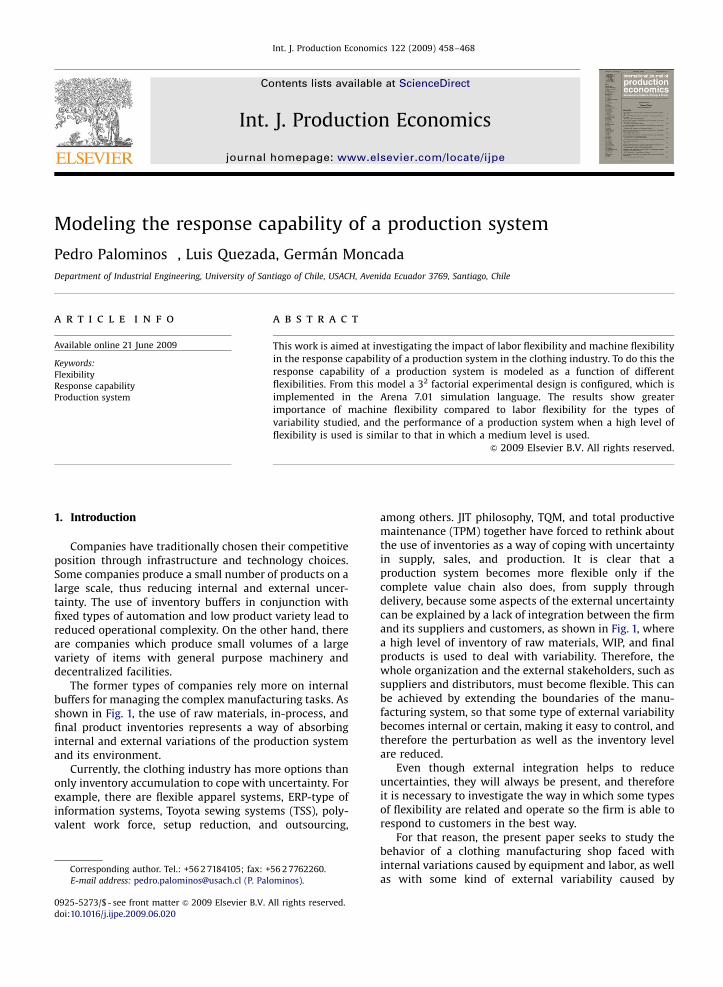
The former types of companies rely more on internalbuffers for managing the complex manufacturing tasks. Asshown in Fig. 1, the use of raw materials, in-process, andfinal product inventories represents a way of absorbinginternal and external variations of the production systemand its environment.

Currently, the clothing industry has more options thanonly inventory accumulation to cope with uncertainty. Forexample, there are flexible apparel systems, ERP-type ofinformation systems, Toyota sewing systems (TSS), poly-valent work force, setup reduction, and outsourcing,

ll rights reserved.

56 2 7762260.

ominos).

among others. JIT philosophy, TQM, and total productivemaintenance (TPM) together have forced to rethink aboutthe use of inventories as a way of coping with uncertaintyin supply, sales, and production. It is clear that aproduction system becomes more flexible only if thecomplete value chain also does, from supply throughdelivery, because some aspects of the external uncertaintycan be explained by a lack of integration between the firmand its suppliers and customers, as shown in Fig. 1, wherea high level of inventory of raw materials, WIP, and finalproducts is used to deal with variability. Therefore, thewhole organization and the external stakeholders, such assuppliers and distributors, must become flexible. This canbe achieved by extending the boundaries of the manu-facturing system, so that some type of external variabilitybecomes internal or certain, making it easy to control, andtherefore the perturbation as well as the inventory levelare reduced.

Even though external integration helps to reduceuncertainties, they will always be present, and thereforeit is necessary to investigate the way in which some typesof flexibility are related and operate so the firm is able torespond to customers in the best way.

For that reason, the present paper seeks to study thebehavior of a clothing manufacturing shop faced withinternal variations caused by equipment and labor, as wellas with some kind of external variability caused by

Page 2

ARTICLE IN PRESS

Raw material

Inventory

FinishedProduct

Inventory

Inventory Inventory

Process

Variability

Products and Processesof

Variabilityof

Equipment and Labor

DemandSupplierVariability

D = S =

PRODUCTION SYSTEM

Variability

S D

Fig. 1. Types of variability in production systems.

Table 1Number and percentage of divulging articles and others on flexibility

during the 1986–2007 period.

Type of content Number of published

articles

Percentage

P. Palominos et al. / Int. J. Production Economics 122 (2009) 458–468 459

changes in demand. For that purpose the productionsystem will be studied with several levels of flexibility inorder to deal with such disturbances. The flexibility can beseen as a fundamental property of the manufacturingsystem (Grubbstrom and Olhager, 1997).

Labor organization 12 34.29

Machinery and production

systems

8 22.86

In-plant applications 5 14.29

Information systems 3 8.57

Strategy 3 8.57

General 3 8.57

CAD 1 2.85

2. On flexibility in the clothing industry

Sethi and Sethi (1990) describe manufacturing flex-ibility as ‘‘y the property of the elements of a system ofintegrating and relating themselves in order to allow theadaptation of production equipment to several manufac-turing tasksy’’. Zelenovic (1982) establishes that flex-ibility of a production system ‘‘y is a measure of itscapacity to adapt to changing environmental conditionsand process requirementsy’’. These definitions, however,are not operational, and the subject of flexibility is farfrom being exhausted as many articles in the literaturehave shown in recent years.

However, in the clothing industry such studies are rare,although the subject and related techniques are com-monly exposed in the divulging literature. In the1986–2007 period nearly 35 articles can be found, aspresented in Table 1, based on the work of Palominos(1996).

First, it is seen that the largest percentage of publica-tions is about labor organization, specifically on cellularmanufacturing work teams, where the goodness offlexible workers is highlighted. Secondly, there are articlesrelated to multiple operation sewing machines (machineflexibility), with unit piece systems (route and productflexibility) which provide much flexibility without speci-fying type and grade. In the third place, there are reportson companies that have chosen one of the two formerapproaches, but they basically describe the way compa-nies work. That is to say, the journalistic approach isunderscored over the technical one.

In the majority of articles the concept of flexibility isthreefold: it means flexible labor, machine flexibility, orroute/mix of product, without a deeper analysis or

discussion of its applicability compared to conventionalsystems.

In more technically oriented literature, the contribu-tions in chronological order are the following:

Tayler (1989) studied the effect on standard unit costper minute of adding one more product to a rigid(inflexible) production line (style change only), thusconcluding that costs will stabilize around the 10th weekwith a cost increment of 15%. Besides, he offersstrategies to improve factory flexibility based ontechnology, better human resource organization, andinfrastructure.

(Stopford and Baden-Fuller (1990) examined the UK’sknitwear industry by discussing strategies to make itmore flexible. They concluded that management andrelations with suppliers and buyers were fundamental.

Robinet (1991), in a project named CEPIFLEX carriedout at CETIH in mid-1985 to develop flexible cells inclothing manufacture under Toyota’s philosophy (TSS),concluded that the most important factor to get a flexibleproduction organization was having multi-skill (function-ally flexible ) workers. Moreover, he states that such asystem would contribute to improve the company’sreaction, but its disadvantage may be investmentrequirements.

Page 3

ARTICLE IN PRESS

External

Flexible Machine

Uncertainty

FlexibleManufacturing Level

Inventory

Lead Time

Internal

Integration

capacityBuffers

Fig. 2. Newman et al. model (Newman et al., 1993).

Table 2Disturbances and responding mechanisms in the clothing industry.

Disturbances Responding mechanisms

External BuffersDemand variation Safety stocks

Supplier variation Excess capacity

Lead time re-scheduling

Internal FlexibilitiesProcess time variation Labor flexibility

Worker absenteeism Machine flexibility

Machine failures

Manufacturing defects

P. Palominos et al. / Int. J. Production Economics 122 (2009) 458–468460

Syssau (1992), in a survey at 18 companies in thetextile and clothing industry, classified the uncertaintysources (mainly external) which affect them. He statesthat flexibility is the answer to the problem. Besides, hedefines the flexibility concept in the same terms as Sethiand Sethi (1990) do by distinguishing two types:one of quantitative or level type (volume flexibility), andone of qualitative or product-based type (product flex-ibility).

Bailey (1993), in a study carried out at 21 clothingcompanies in the USA on organizational innovations inthis sector, contrasted mass production with team-basedwork approach. He concluded that flexible specializationleads to greater variety and faster changes, and thatautomation improves communications between suppliersand customers.

Baker (1993) analyzed the restructuring process of theclothing and textile industry in the UK by centeringspecifically on new technologies, labor flexibility, andsubcontracting. He considered labor flexibility in Atkin-son’s terms (Atkinson, 1984), that is: (a) functionally and(b) numerically. Baker concluded that case (a) occurred ingreater proportion in small companies, since they haveless personnel and must perform more different tasksthan large companies. On the other hand, in bigcompanies specialization remains longer and creation ofnew jobs takes place by the incorporation of moreadvanced equipment. Similarly, small companies usemore numerical flexibility than bigger ones.

Taplin and Winterton (1995), in a study of companiesin the USA and the UK, concluded, among other things,that increased flexibility in the clothing industry can beachieved by limiting design operations, and in some casescutting operations, in the company itself, while subcon-tracting assembly with many small shops.

Dana and Hamilton (2007) examined the New Zealandapparel firm by discussing strategies to make it moreflexible. They discovered that although at least partialoffshore sourcing may be a viable option for many smallapparel firms.

Kalaoglu and Saricam (2007) propose a simulationmodel of modular manufacturing to study the productiv-ity of the system, varying the number of workers within acell. They even found variations in productivity when thenumber of workers is changed, but they did not make adistinction between numerical flexibility (number work-ers) and functional flexibility (polyvalence).

It is seen that research on flexibility in the clothingindustry deals mainly with on-site studies about strate-gies to be followed based on the experience of largecompanies which one way or another appear in most ofthe cited cases. The only authors that mention flexibilityare Tayler (1989), Robinet (1991), Syssau (1992), andKalaoglu and Saricam (2007) even though it is not thesubject of the studies. We can therefore conclude thatmanufacturing flexibility in the clothing industry doesrequire human and technological resources; however themanagement, the dynamics, and the flexibility principleshave not been investigated. Therefore, in the presentarticle we study the behavior of flexibility in the responsecapability of a production system. For this, we consider

two kinds of strategies: machine- and labor-based flex-ibility.

3. A conceptual model and planning the experiment

3.1. A Newman et al. model

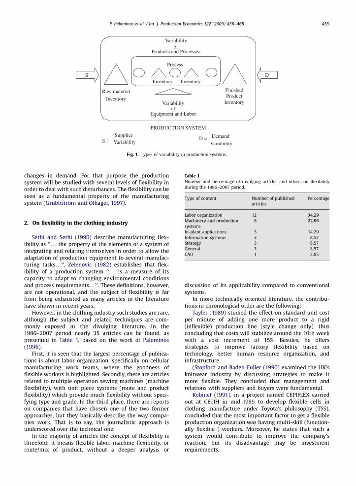
Newman et al. (1993) present a dynamic balancemodel between variability that affects the productionsystem and the way in which the system inhibits thatvariability, by means of inventory and the system’sflexibility. This model proposes a balance (see Fig. 2),where on the one hand there is the uncertainty, internal orexternal, and on the other hand the integration and theflexibility of machine or resources.

According to the proposed conceptual model, thefactors that may affect response capability in a sewingshop can be classified into two main groups: (a) systemdisturbance, either internal or external and (b) theresponding mechanisms, such as buffers or elements thatgive flexibility to the manufacturing shop, as presented inTable 2.

3.2. Experimental design

From the above, a global experimental structure wasdesigned which considers the different kinds of distur-bances and flexibility factors, namely machine and labor,in three levels, as presented in Table 3. The disturbancesconsidered have both an internal and an external nature,

Page 4

ARTICLE IN PRESS

Table 3Experimental design structure.

Environment (disturbances) Flexibility

Internal and external Machine Labor

H M L H M L

Process time+absenteeism+machine failures+demand variations

H ¼ high level; M ¼ medium level; L ¼ low level.

Table 4Base matrix for the experiments.

Experiment number Machine flexibility Labor flexibility

1 L L

2 L M

3 L H

4 M L

5 M M

6 M H

7 H L

8 H M

9 H H

P. Palominos et al. / Int. J. Production Economics 122 (2009) 458–468 461

where the internal ones are variability in processing time,absenteeism, and machine breakdown, while the externalones correspond to the variability of the demand.

The labor flexibility that will be used in the develop-ment of the experimental design is functional flexibility,which is the most representative and common in theapparel industry (Tayler, 1989; Syssau, 1992) also know asthe polyvalence of the workers, where the boundariesexpand in the different work places, so that the workershave multiple competences. In particular, this approach isorientated at the rotation of different work places and/ormachines (Stewart et al., 1994). In this way labor flexibilitywill be expressed as the number of machines that aworker is able to operate without a major effort.

On the other hand, machine flexibility means that amachine can perform different operations and producedifferent products without a major set-up when changingfrom one piece to another. According to Sethi and Sethi(1990) this type of flexibility can be measured in terms ofnumber of operations. However, Malhotra and Ritzman(1990) and Gupta (1993) define it in terms of the numberof product types. In the present research the secondoption is used.

The response capability will be measured in terms ofthe number of manufactured pieces, the total flow time ofbatches in the shop and machines, and labor performance.Machines and labor performance are measured as themean of the percentage of use of all the machines andworkers in the production system.

The selected factors are tested at three levels: high (H),medium (M) and low (L). Then, a matrix of experiments isgenerated presented in Table 4. The factor levels areindicated below and are based on the Spanish clothingindustry.

(a)

Labor flexibility (multi-skill worker):� High level ¼ 4 sewing machines.� Medium level ¼ 2 sewing machines.� Low level ¼ 1 sewing machine.

(b)

Machine flexibility:� High level ¼ 3 different products.� Medium level ¼ 2 different products.� Low level ¼ 1 product only.

This means that, given the external and internaldisturbances, nine simulation experiments have to berun, as presented in Table 4, i.e., the first experiment witha low level of machinery (L) and labor flexibility (L); thesecond experiment with a low level of machinery and a

medium level of labor flexibility, and so on. Eachexperiment has five replications.

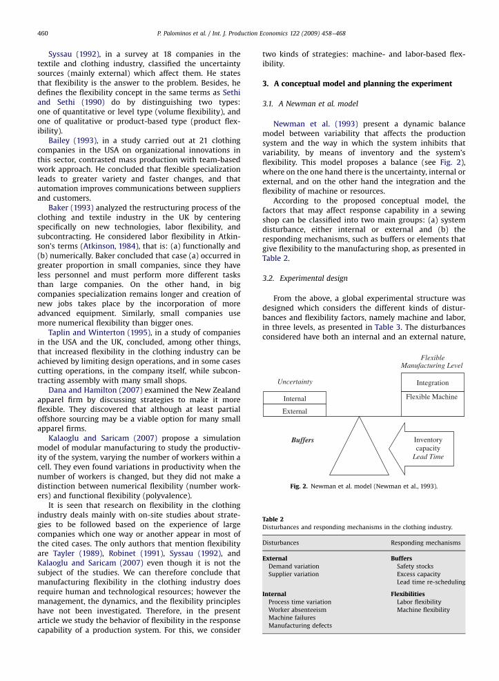
The design of the production system to be simulatedusing Arena 7.01 is composed of three manufacturing lineswhich produce sportswear, because of their simplicity andthe number of operations that are performed. The threeproduction lines have the same number of machines andworkers each (four); thus, the manufacturing shop iscomposed of 12 machines and 12 workers and manufac-tures three products (A, B and C), with a theoreticalproduction capacity of eight batches on each line per day.This work uses the technical information about theproducts (operations, machine types, operation types,and process times) and the probability distributions formachine failures and worker absenteeism proposed byPalominos (1996).

As an example, Fig. 3 shows a production systemhaving a medium level of machine and labor flexibility,where the machines can manufacture two products. Themachines of line 1 can manufacture type A and Bproducts; the machines of line 2 can manufacture type Aand C products, and the machines of line 3 canmanufacture type B and C products. Labor flexibility inthe medium level means that each worker is able tooperate two types of machines. Fig. 3 shows that sixworkers are able to operate machines of types 1 and 2(Area 1) and the other six are able to operate machines oftypes 3 and 4 (Area 2).

3.2.1. Assumptions and considerations of the models to

simulate

The assumptions of the above system design are thefollowing:

(a)

The machine only operates when a worker has beenassigned and the job is available for processing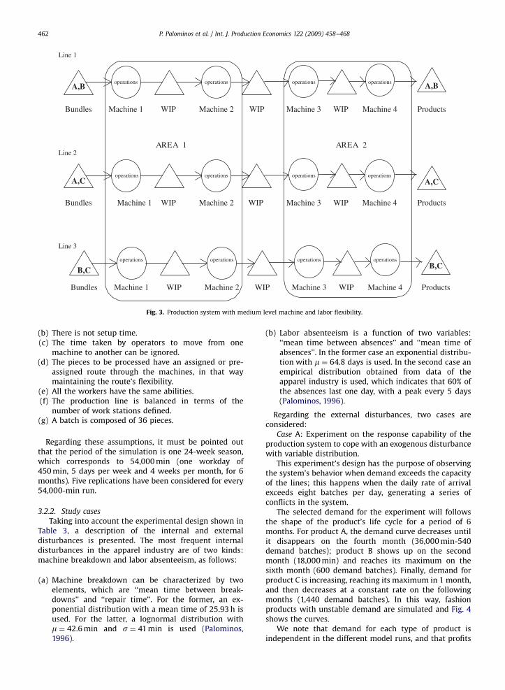

Page 5

ARTICLE IN PRESS

operations

WIP Machine 1 Machine 2Bundles

operationsA,B

operations

Machine 4

operations

Machine 3

operations

WIP Machine 2Bundles

operations

Machine 4

operations

Machine 3WIP

operations

WIP Machine 1 Machine 2Bundles

operations

Machine 4

operations

Machine 3

operations

operations

A,C

A,B

A,C

B,C B,C

Machine 1

WIP

WIP

WIP

WIP

WIP

Products

Products

Products

2AERA1AERA

Line 1

Line 2

Line 3

Fig. 3. Production system with medium level machine and labor flexibility.

P. Palominos et al. / Int. J. Production Economics 122 (2009) 458–468462

(b)

There is not setup time. (c) The time taken by operators to move from one

machine to another can be ignored.

(d) The pieces to be processed have an assigned or pre-

assigned route through the machines, in that waymaintaining the route’s flexibility.

(e)

All the workers have the same abilities. (f) The production line is balanced in terms of the

number of work stations defined.

(g) A batch is composed of 36 pieces.

Regarding these assumptions, it must be pointed outthat the period of the simulation is one 24-week season,which corresponds to 54,000 min (one workday of450 min, 5 days per week and 4 weeks per month, for 6months). Five replications have been considered for every54,000-min run.

3.2.2. Study cases

Taking into account the experimental design shown inTable 3, a description of the internal and externaldisturbances is presented. The most frequent internaldisturbances in the apparel industry are of two kinds:machine breakdown and labor absenteeism, as follows:

(a)

Machine breakdown can be characterized by twoelements, which are ‘‘mean time between break-downs’’ and ‘‘repair time’’. For the former, an ex-ponential distribution with a mean time of 25.93 h isused. For the latter, a lognormal distribution withm ¼ 42.6 min and s ¼ 41 min is used (Palominos,1996).

(b)

Labor absenteeism is a function of two variables:‘‘mean time between absences’’ and ‘‘mean time ofabsences’’. In the former case an exponential distribu-tion with m ¼ 64.8 days is used. In the second case anempirical distribution obtained from data of theapparel industry is used, which indicates that 60% ofthe absences last one day, with a peak every 5 days(Palominos, 1996).

Regarding the external disturbances, two cases areconsidered:

Case A: Experiment on the response capability of theproduction system to cope with an exogenous disturbancewith variable distribution.

This experiment’s design has the purpose of observingthe system’s behavior when demand exceeds the capacityof the lines; this happens when the daily rate of arrivalexceeds eight batches per day, generating a series ofconflicts in the system.

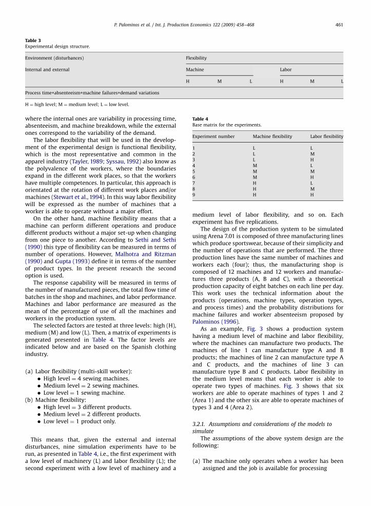
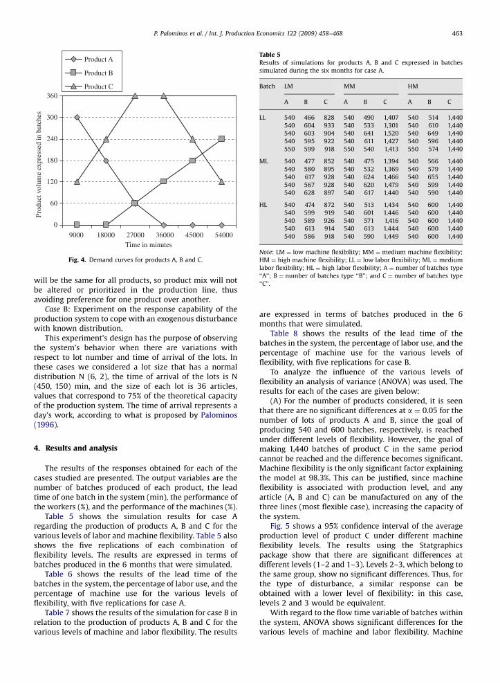
The selected demand for the experiment will followsthe shape of the product’s life cycle for a period of 6months. For product A, the demand curve decreases untilit disappears on the fourth month (36,000 min-540demand batches); product B shows up on the secondmonth (18,000 min) and reaches its maximum on thesixth month (600 demand batches). Finally, demand forproduct C is increasing, reaching its maximum in 1 month,and then decreases at a constant rate on the followingmonths (1,440 demand batches). In this way, fashionproducts with unstable demand are simulated and Fig. 4shows the curves.

We note that demand for each type of product isindependent in the different model runs, and that profits

Page 6

ARTICLE IN PRESS

0

60

120

180

240

300

360

9000

Prod

uct v

olum

e ex

pres

sed

in b

atch

es

Product A

Product B

Product C

18000 27000 36000 45000 54000Time in minutes

Fig. 4. Demand curves for products A, B and C.

Table 5Results of simulations for products A, B and C expressed in batches

simulated during the six months for case A.

Batch LM MM HM

A B C A B C A B C

LL 540 466 828 540 490 1,407 540 514 1,440

540 604 933 540 533 1,301 540 610 1,440

540 603 904 540 641 1,520 540 649 1,440

540 595 922 540 611 1,427 540 596 1,440

550 599 918 550 540 1,413 550 574 1,440

ML 540 477 852 540 475 1,394 540 566 1,440

540 580 895 540 532 1,369 540 579 1,440

540 617 928 540 624 1,466 540 655 1,440

540 567 928 540 620 1,479 540 599 1,440

540 628 897 540 617 1,440 540 590 1,440

HL 540 474 872 540 513 1,434 540 600 1,440

540 599 919 540 601 1,446 540 600 1,440

540 589 926 540 571 1,416 540 600 1,440

540 613 914 540 613 1,444 540 600 1,440

540 586 918 540 590 1,449 540 600 1,440

Note: LM ¼ low machine flexibility; MM ¼ medium machine flexibility;

HM ¼ high machine flexibility; LL ¼ low labor flexibility; ML ¼ medium

labor flexibility; HL ¼ high labor flexibility; A ¼ number of batches type

‘‘A’’; B ¼ number of batches type ‘‘B’’; and C ¼ number of batches type

‘‘C’’.

P. Palominos et al. / Int. J. Production Economics 122 (2009) 458–468 463

will be the same for all products, so product mix will notbe altered or prioritized in the production line, thusavoiding preference for one product over another.

Case B: Experiment on the response capability of theproduction system to cope with an exogenous disturbancewith known distribution.

This experiment’s design has the purpose of observingthe system’s behavior when there are variations withrespect to lot number and time of arrival of the lots. Inthese cases we considered a lot size that has a normaldistribution N (6, 2), the time of arrival of the lots is N(450, 150) min, and the size of each lot is 36 articles,values that correspond to 75% of the theoretical capacityof the production system. The time of arrival represents aday’s work, according to what is proposed by Palominos(1996).

4. Results and analysis

The results of the responses obtained for each of thecases studied are presented. The output variables are thenumber of batches produced of each product, the leadtime of one batch in the system (min), the performance ofthe workers (%), and the performance of the machines (%).

Table 5 shows the simulation results for case Aregarding the production of products A, B and C for thevarious levels of labor and machine flexibility. Table 5 alsoshows the five replications of each combination offlexibility levels. The results are expressed in terms ofbatches produced in the 6 months that were simulated.

Table 6 shows the results of the lead time of thebatches in the system, the percentage of labor use, and thepercentage of machine use for the various levels offlexibility, with five replications for case A.

Table 7 shows the results of the simulation for case B inrelation to the production of products A, B and C for thevarious levels of machine and labor flexibility. The results

are expressed in terms of batches produced in the 6months that were simulated.

Table 8 shows the results of the lead time of thebatches in the system, the percentage of labor use, and thepercentage of machine use for the various levels offlexibility, with five replications for case B.

To analyze the influence of the various levels offlexibility an analysis of variance (ANOVA) was used. Theresults for each of the cases are given below:

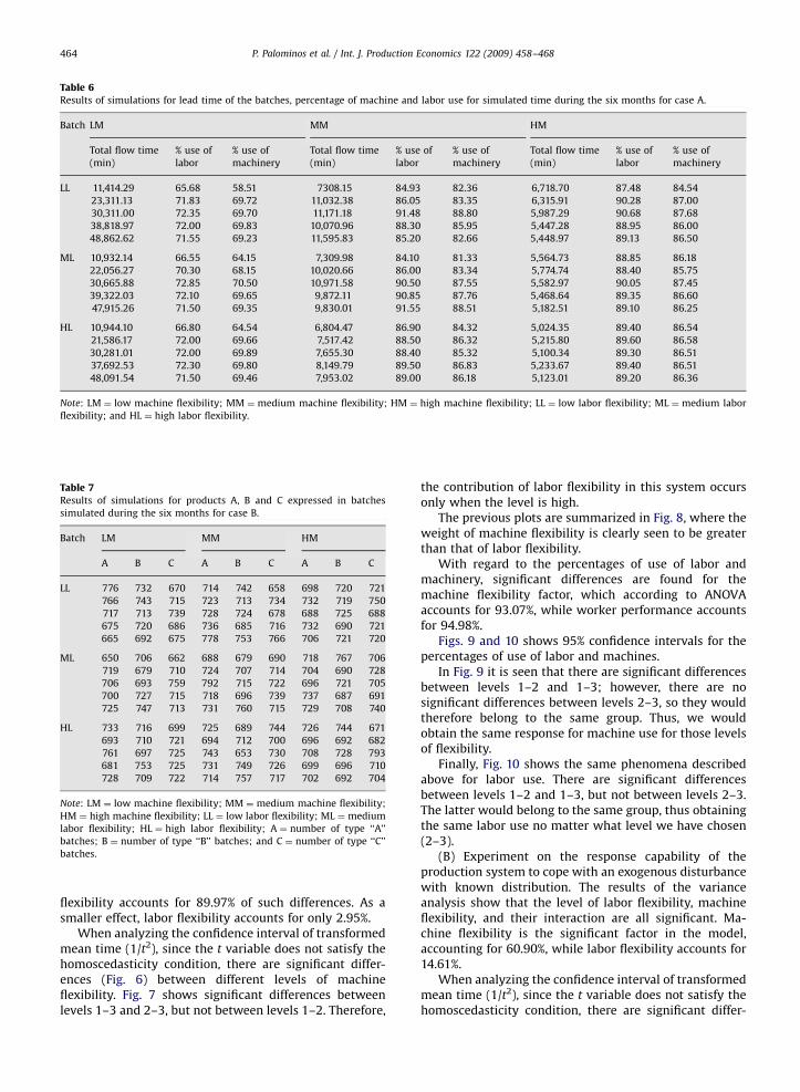
(A) For the number of products considered, it is seenthat there are no significant differences at a ¼ 0.05 for thenumber of lots of products A and B, since the goal ofproducing 540 and 600 batches, respectively, is reachedunder different levels of flexibility. However, the goal ofmaking 1,440 batches of product C in the same periodcannot be reached and the difference becomes significant.Machine flexibility is the only significant factor explainingthe model at 98.3%. This can be justified, since machineflexibility is associated with production level, and anyarticle (A, B and C) can be manufactured on any of thethree lines (most flexible case), increasing the capacity ofthe system.

Fig. 5 shows a 95% confidence interval of the averageproduction level of product C under different machineflexibility levels. The results using the Statgraphicspackage show that there are significant differences atdifferent levels (1–2 and 1–3). Levels 2–3, which belong tothe same group, show no significant differences. Thus, forthe type of disturbance, a similar response can beobtained with a lower level of flexibility: in this case,levels 2 and 3 would be equivalent.

With regard to the flow time variable of batches withinthe system, ANOVA shows significant differences for thevarious levels of machine and labor flexibility. Machine

Page 7

ARTICLE IN PRESS

Table 6Results of simulations for lead time of the batches, percentage of machine and labor use for simulated time during the six months for case A.

Batch LM MM HM

Total flow time

(min)

% use of

labor

% use of

machinery

Total flow time

(min)

% use of

labor

% use of

machinery

Total flow time

(min)

% use of

labor

% use of

machinery

LL 11,414.29 65.68 58.51 7308.15 84.93 82.36 6,718.70 87.48 84.54

23,311.13 71.83 69.72 11,032.38 86.05 83.35 6,315.91 90.28 87.00

30,311.00 72.35 69.70 11,171.18 91.48 88.80 5,987.29 90.68 87.68

38,818.97 72.00 69.83 10,070.96 88.30 85.95 5,447.28 88.95 86.00

48,862.62 71.55 69.23 11,595.83 85.20 82.66 5,448.97 89.13 86.50

ML 10,932.14 66.55 64.15 7,309.98 84.10 81.33 5,564.73 88.85 86.18

22,056.27 70.30 68.15 10,020.66 86.00 83.34 5,774.74 88.40 85.75

30,665.88 72.85 70.50 10,971.58 90.50 87.55 5,582.97 90.05 87.45

39,322.03 72.10 69.65 9,872.11 90.85 87.76 5,468.64 89.35 86.60

47,915.26 71.50 69.35 9,830.01 91.55 88.51 5,182.51 89.10 86.25

HL 10,944.10 66.80 64.54 6,804.47 86.90 84.32 5,024.35 89.40 86.54

21,586.17 72.00 69.66 7,517.42 88.50 86.32 5,215.80 89.60 86.58

30,281.01 72.00 69.89 7,655.30 88.40 85.32 5,100.34 89.30 86.51

37,692.53 72.30 69.80 8,149.79 89.50 86.83 5,233.67 89.40 86.51

48,091.54 71.50 69.46 7,953.02 89.00 86.18 5,123.01 89.20 86.36

Note: LM ¼ low machine flexibility; MM ¼ medium machine flexibility; HM ¼ high machine flexibility; LL ¼ low labor flexibility; ML ¼medium labor

flexibility; and HL ¼ high labor flexibility.

Table 7Results of simulations for products A, B and C expressed in batches

simulated during the six months for case B.

Batch LM MM HM

A B C A B C A B C

LL 776 732 670 714 742 658 698 720 721

766 743 715 723 713 734 732 719 750

717 713 739 728 724 678 688 725 688

675 720 686 736 685 716 732 690 721

665 692 675 778 753 766 706 721 720

ML 650 706 662 688 679 690 718 767 706

719 679 710 724 707 714 704 690 728

706 693 759 792 715 722 696 721 705

700 727 715 718 696 739 737 687 691

725 747 713 731 760 715 729 708 740

HL 733 716 699 725 689 744 726 744 671

693 710 721 694 712 700 696 692 682

761 697 725 743 653 730 708 728 793

681 753 725 731 749 726 699 696 710

728 709 722 714 757 717 702 692 704

Note: LM ¼ low machine flexibility; MM ¼ medium machine flexibility;

HM ¼ high machine flexibility; LL ¼ low labor flexibility; ML ¼ medium

labor flexibility; HL ¼ high labor flexibility; A ¼ number of type ‘‘A’’

batches; B ¼ number of type ‘‘B’’ batches; and C ¼ number of type ‘‘C’’

batches.

P. Palominos et al. / Int. J. Production Economics 122 (2009) 458–468464

flexibility accounts for 89.97% of such differences. As asmaller effect, labor flexibility accounts for only 2.95%.

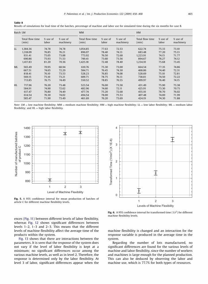
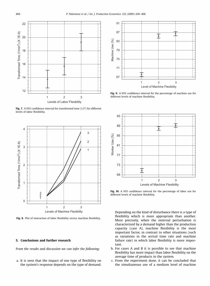
When analyzing the confidence interval of transformedmean time (1/t2), since the t variable does not satisfy thehomoscedasticity condition, there are significant differ-ences (Fig. 6) between different levels of machineflexibility. Fig. 7 shows significant differences betweenlevels 1–3 and 2–3, but not between levels 1–2. Therefore,

the contribution of labor flexibility in this system occursonly when the level is high.

The previous plots are summarized in Fig. 8, where theweight of machine flexibility is clearly seen to be greaterthan that of labor flexibility.

With regard to the percentages of use of labor andmachinery, significant differences are found for themachine flexibility factor, which according to ANOVAaccounts for 93.07%, while worker performance accountsfor 94.98%.

Figs. 9 and 10 shows 95% confidence intervals for thepercentages of use of labor and machines.

In Fig. 9 it is seen that there are significant differencesbetween levels 1–2 and 1–3; however, there are nosignificant differences between levels 2–3, so they wouldtherefore belong to the same group. Thus, we wouldobtain the same response for machine use for those levelsof flexibility.

Finally, Fig. 10 shows the same phenomena describedabove for labor use. There are significant differencesbetween levels 1–2 and 1–3, but not between levels 2–3.The latter would belong to the same group, thus obtainingthe same labor use no matter what level we have chosen(2–3).

(B) Experiment on the response capability of theproduction system to cope with an exogenous disturbancewith known distribution. The results of the varianceanalysis show that the level of labor flexibility, machineflexibility, and their interaction are all significant. Ma-chine flexibility is the significant factor in the model,accounting for 60.90%, while labor flexibility accounts for14.61%.

When analyzing the confidence interval of transformedmean time (1/t2), since the t variable does not satisfy thehomoscedasticity condition, there are significant differ-

Page 8

ARTICLE IN PRESS

Table 8Results of simulations for lead time of the batches, percentage of machine and labor use for simulated time during the six months for case B.

Batch LM MM HM

Total flow time

(min)

% use of

labor

% use of

machinery

Total flow time

(min)

% use of

labor

% use of

machinery

Total flow time

(min)

% use of

labor

% use of

machinery

LL 1,384.36 74.78 74.78 1,054.85 77.63 72.53 622.74 75.33 73.10

1,318.09 76.85 76.21 896.07 78.40 74.13 683.48 77.20 75.13

931.41 75.05 73.88 773.92 76.50 72.68 1,223.91 74.15 71.77

690.86 75.93 71.53 749.41 73.60 73.56 894.67 76.27 74.12

1,417.83 81.20 70.36 1,425.18 72.48 78.40 1,234.10 75.68 73.45

ML 565.49 70.95 68.94 610.76 75.30 73.00 664.54 77.35 74.86

667.51 74.65 72.29 584.71 76.45 74.30 468.86 74.40 72.31

818.41 76.10 73.53 528.23 76.85 74.08 528.69 75.10 72.81

569.15 75.10 73.21 609.71 78.75 76.13 738.81 74.50 72.22

713.85 76.75 74.49 550.52 78.85 76.55 499.97 76.40 74.15

HL 717.96 76.20 73.48 523.54 76.00 73.58 431.49 75.90 73.38

584.91 74.90 72.62 482.96 74.60 72.11 425.91 73.30 70.75

617.47 76.80 74.49 477.74 75.20 72.68 455.10 78.70 76.02

614.54 76.30 74.02 494.54 78.00 75.53 407.48 74.00 71.99

585.47 71.90 73.49 461.69 76.20 73.69 424.19 74.30 71.88

Note: LM ¼ low machine flexibility; MM ¼ medium machine flexibility; HM ¼ high machine flexibility; LL ¼ low labor flexibility; ML ¼ medium labor

flexibility; and HL ¼ high labor flexibility.

1

Level of Machine Flexibility

890

990

1090

1190

1290

1390

1490

Num

ber o

f man

ufac

ture

d ba

tche

sof

pro

duct

C

2 3

Fig. 5. A 95% confidence interval for mean production of batches of

article C for different machine flexibility levels. 1Levels of Machine Flexibility

0

1

2

3

4

Tran

sfor

med

Tim

e (1

/min

2 ) (X

1E

-8)

2 3

Fig. 6. A 95% confidence interval for transformed time (1/t2) for different

machine flexibility levels.

P. Palominos et al. / Int. J. Production Economics 122 (2009) 458–468 465

ences (Fig. 11) between different levels of labor flexibility,whereas Fig. 12 shows significant differences betweenlevels 1–2, 1–3 and 2–3. This means that the differentlevels of machine flexibility affect the average time of theproducts within the system.

Fig. 13 shows that there are interactions between theparameters. It is seen that the response of the system doesnot vary if the level of labor flexibility is kept at aminimum; no significant differences occur among thevarious machine levels, as well as in level 2. Therefore, theresponse is determined only by the labor flexibility. Atlevel 3 of labor, significant differences appear when the

machine flexibility is changed and an interaction for theresponse variable is produced in the average time in thesystem.

Regarding the number of lots manufactured, nosignificant differences are found for the various levels ofmachine and labor flexibility, since the number of workersand machines is large enough for the planned production.This can also be deduced by observing the labor andmachine use, which is 77.7% for both types of resources.

Page 9

ARTICLE IN PRESS

1Levels of Labor Flexibility

12

14

16

18

20

22

Tran

sfor

med

Tim

e (1

/min

2 ) (X

1E

-9)

2 3

Fig. 7. A 95% confidence interval for transformed time (1/t2) for different

levels of labor flexibility.

1Levels of Machine Flexibility

0

1

2

3

4

Tran

sfor

med

Tim

e (1

/min

2 ) (X

1E

-8)

1

1

2

2

3

3

2 3

Fig. 8. Plot of interaction of labor flexibility versus machine flexibility.

1Level of Machine Flexibility

67

71

75

79

83

87

91

Mac

hine

Use

(%)

2 3

Fig. 9. A 95% confidence interval for the percentage of machine use for

different levels of machine flexibility.

1Levels of Machine Flexibility

69

73

77

81

85

89

93W

orke

r Use

(%)

2 3

Fig. 10. A 95% confidence interval for the percentage of labor use for

different levels of machine flexibility.

P. Palominos et al. / Int. J. Production Economics 122 (2009) 458–468466

5. Conclusions and further research

From the results and discussion we can infer the following:

a.

It is seen that the impact of one type of flexibility onthe system’s response depends on the type of demand.

Depending on the kind of disturbance there is a type offlexibility which is more appropriate than another.More precisely, when the external perturbation ischaracterized by a demand higher than the productioncapacity (case A), machine flexibility is the mostimportant factor, in contrast to other situations (suchas variations in the arrival time rate and machinefailure rate) in which labor flexibility is more impor-tant.

b.

For cases A and B it is possible to see that machineflexibility has more impact than labor flexibility on theaverage time of products in the system.

c.

From the experiment done, it can be concluded thatthe simultaneous use of a medium level of machine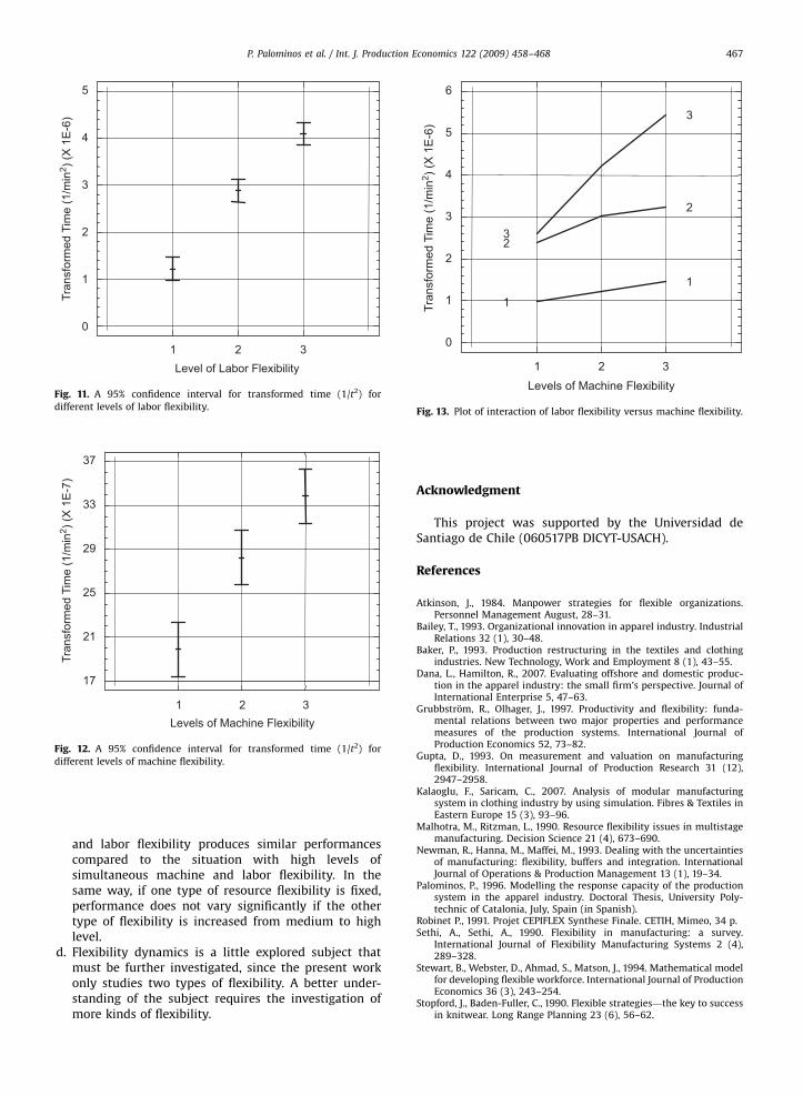

Page 10

ARTICLE IN PRESS

1 2 3Level of Labor Flexibility

0

1

2

3

4

5

Tra

nsfo

rmed

Tim

e (1

/min

2 ) (X

1E

-6)

Fig. 11. A 95% confidence interval for transformed time (1/t2) for

different levels of labor flexibility.

1 2 3Levels of Machine Flexibility

17

21

25

29

33

37

Tran

sfor

med

Tim

e (1

/min

2 ) (X

1E

-7)

Fig. 12. A 95% confidence interval for transformed time (1/t2) for

different levels of machine flexibility.

1 2 3Levels of Machine Flexibility

0

1

2

3

4

5

6

1

1

2

2

3

3

Tran

sfor

med

Tim

e (1

/min

2 ) (X

1E

-6)

Fig. 13. Plot of interaction of labor flexibility versus machine flexibility.

P. Palominos et al. / Int. J. Production Economics 122 (2009) 458–468 467

and labor flexibility produces similar performancescompared to the situation with high levels ofsimultaneous machine and labor flexibility. In thesame way, if one type of resource flexibility is fixed,performance does not vary significantly if the othertype of flexibility is increased from medium to highlevel.

d.

Flexibility dynamics is a little explored subject thatmust be further investigated, since the present workonly studies two types of flexibility. A better under-standing of the subject requires the investigation ofmore kinds of flexibility.

Acknowledgment

This project was supported by the Universidad deSantiago de Chile (060517PB DICYT-USACH).

References

Atkinson, J., 1984. Manpower strategies for flexible organizations.Personnel Management August, 28–31.

Bailey, T., 1993. Organizational innovation in apparel industry. IndustrialRelations 32 (1), 30–48.

Baker, P., 1993. Production restructuring in the textiles and clothingindustries. New Technology, Work and Employment 8 (1), 43–55.

Dana, L., Hamilton, R., 2007. Evaluating offshore and domestic produc-tion in the apparel industry: the small firm’s perspective. Journal ofInternational Enterprise 5, 47–63.

Grubbstrom, R., Olhager, J., 1997. Productivity and flexibility: funda-mental relations between two major properties and performancemeasures of the production systems. International Journal ofProduction Economics 52, 73–82.

Gupta, D., 1993. On measurement and valuation on manufacturingflexibility. International Journal of Production Research 31 (12),2947–2958.

Kalaoglu, F., Saricam, C., 2007. Analysis of modular manufacturingsystem in clothing industry by using simulation. Fibres & Textiles inEastern Europe 15 (3), 93–96.

Malhotra, M., Ritzman, L., 1990. Resource flexibility issues in multistagemanufacturing. Decision Science 21 (4), 673–690.

Newman, R., Hanna, M., Maffei, M., 1993. Dealing with the uncertaintiesof manufacturing: flexibility, buffers and integration. InternationalJournal of Operations & Production Management 13 (1), 19–34.

Palominos, P., 1996. Modelling the response capacity of the productionsystem in the apparel industry. Doctoral Thesis, University Poly-technic of Catalonia, July, Spain (in Spanish).

Robinet P., 1991. Projet CEPIFLEX Synthese Finale. CETIH, Mimeo, 34 p.Sethi, A., Sethi, A., 1990. Flexibility in manufacturing: a survey.

International Journal of Flexibility Manufacturing Systems 2 (4),289–328.

Stewart, B., Webster, D., Ahmad, S., Matson, J., 1994. Mathematical modelfor developing flexible workforce. International Journal of ProductionEconomics 36 (3), 243–254.

Stopford, J., Baden-Fuller, C., 1990. Flexible strategies—the key to successin knitwear. Long Range Planning 23 (6), 56–62.

Page 11

ARTICLE IN PRESS

P. Palominos et al. / Int. J. Production Economics 122 (2009) 458–468468

Syssau, J., 1992. Repondre a l’incertitude par la flexibilite: Le cas de 18entreprises de la filiere textile habillement. Gestion 2000 8(4), 11–28.

Taplin, I., Winterton, J., 1995. New clothes from old techniques:restructuring and flexibility in the US and UK clothing industries.Industrial and Corporate Change 4 (3), 615–638.

Tayler, D., 1989. Managing for production flexibility in the clothingindustry. Textile Outlook International September, 63–84.

Zelenovic, D., 1982. Flexibility—a condition for effective productionsystem. International Journal of production Research 20 (3),319–337.