arXiv:1107.2022v1 [cond-mat.mes-hall] 11 Jul 2011 Modeling the mechanics of amorphous solids at different length and time scales D. Rodney 1 , A. Tanguy 2 , D. Vandembroucq 3 1 Laboratoire Science et Ing´ enierie des Mat´ eriaux et Proc´ ed´ es, Grenoble INP, UJF, CNRS, Domaine Universitaire BP 46, F38402 Saint Martin d’H` eres, France 2 Laboratoire de Physique de la Mati` ere Condens´ ee et Nanostructures, Universit´ e Lyon 1, Domaine Scientifique de la Doua, F69622 Villeurbanne, France 3 Laboratoire Physique et M´ ecanique des Milieux H´ et´ erog` enes, CNRS/ESPCI/UPMC/Universit´ e Paris 7 Diderot, 10 rue Vauquelin, F75231 Paris, France E-mail: [email protected] Abstract. We review the recent literature on the simulation of the structure and deformation of amorphous glasses, including oxide and metallic glasses. We consider simulations at different length and time scales. At the nanometer scale, we review studies based on atomistic simulations, with a particular emphasis on the role of the potential energy landscape and of the temperature. At the micrometer scale, we present the different mesoscopic models of amorphous plasticity and show the relation between shear banding and the type of disorder and correlations (e.g. elastic) included in the models. At the macroscopic range, we review the different constitutive laws used in finite element simulations. We end the review by a critical discussion on the opportunities and challenges offered by multiscale modeling and transfer of information between scales to study amorphous plasticity. PACS numbers: 62.20.-x,81.05.Kf, 83.10.-y Submitted to: Modelling Simulation Mater. Sci. Eng.

Welcome message from author
This document is posted to help you gain knowledge. Please leave a comment to let me know what you think about it! Share it to your friends and learn new things together.
Transcript
arX
iv:1
107.
2022
v1 [
cond
-mat
.mes
-hal
l] 1
1 Ju
l 201
1 Modeling the mechanics of amorphous solids at
different length and time scales
D. Rodney1, A. Tanguy2, D. Vandembroucq3
1Laboratoire Science et Ingenierie des Materiaux et Procedes, Grenoble INP, UJF,
CNRS, Domaine Universitaire BP 46, F38402 Saint Martin d’Heres, France2Laboratoire de Physique de la Matiere Condensee et Nanostructures, Universite
Lyon 1, Domaine Scientifique de la Doua, F69622 Villeurbanne, France3Laboratoire Physique et Mecanique des Milieux Heterogenes,
CNRS/ESPCI/UPMC/Universite Paris 7 Diderot, 10 rue Vauquelin, F75231 Paris,
France
E-mail: [email protected]
Abstract. We review the recent literature on the simulation of the structure and
deformation of amorphous glasses, including oxide and metallic glasses. We consider
simulations at different length and time scales. At the nanometer scale, we review
studies based on atomistic simulations, with a particular emphasis on the role of
the potential energy landscape and of the temperature. At the micrometer scale, we
present the different mesoscopic models of amorphous plasticity and show the relation
between shear banding and the type of disorder and correlations (e.g. elastic) included
in the models. At the macroscopic range, we review the different constitutive laws
used in finite element simulations. We end the review by a critical discussion on the
opportunities and challenges offered by multiscale modeling and transfer of information
between scales to study amorphous plasticity.
PACS numbers: 62.20.-x,81.05.Kf, 83.10.-y
Submitted to: Modelling Simulation Mater. Sci. Eng.
Modeling the mechanics of amorphous solids at different length and time scales 2
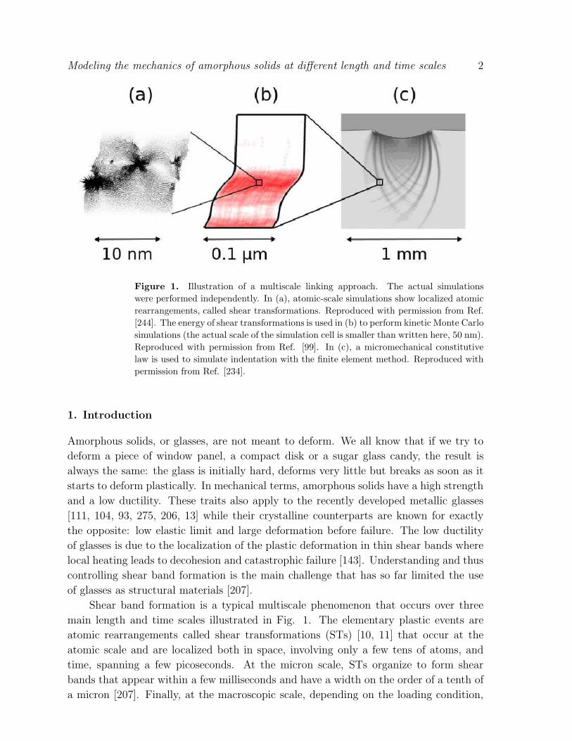
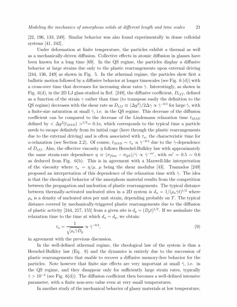
Figure 1. Illustration of a multiscale linking approach. The actual simulations
were performed independently. In (a), atomic-scale simulations show localized atomic
rearrangements, called shear transformations. Reproduced with permission from Ref.
[244]. The energy of shear transformations is used in (b) to perform kinetic Monte Carlo
simulations (the actual scale of the simulation cell is smaller than written here, 50 nm).
Reproduced with permission from Ref. [99]. In (c), a micromechanical constitutive
law is used to simulate indentation with the finite element method. Reproduced with
permission from Ref. [234].
1. Introduction
Amorphous solids, or glasses, are not meant to deform. We all know that if we try to
deform a piece of window panel, a compact disk or a sugar glass candy, the result is
always the same: the glass is initially hard, deforms very little but breaks as soon as it
starts to deform plastically. In mechanical terms, amorphous solids have a high strength
and a low ductility. These traits also apply to the recently developed metallic glasses
[111, 104, 93, 275, 206, 13] while their crystalline counterparts are known for exactly
the opposite: low elastic limit and large deformation before failure. The low ductility
of glasses is due to the localization of the plastic deformation in thin shear bands where
local heating leads to decohesion and catastrophic failure [143]. Understanding and thus
controlling shear band formation is the main challenge that has so far limited the use
of glasses as structural materials [207].
Shear band formation is a typical multiscale phenomenon that occurs over three
main length and time scales illustrated in Fig. 1. The elementary plastic events are
atomic rearrangements called shear transformations (STs) [10, 11] that occur at the
atomic scale and are localized both in space, involving only a few tens of atoms, and
time, spanning a few picoseconds. At the micron scale, STs organize to form shear
bands that appear within a few milliseconds and have a width on the order of a tenth of
a micron [207]. Finally, at the macroscopic scale, depending on the loading condition,
Modeling the mechanics of amorphous solids at different length and time scales 3
either a single shear band forms as in tension test, or several shear bands form and
interact, in case of confined plasticity as in indentation tests [234].
The study of plasticity in amorphous solids has greatly benefited from computer
simulations; probably more than crystalline solids, because of the lack of experimental
device able to identify plastic events in glasses, in the way electron microscopy images
dislocations in crystals and also because the intrinsic brittleness of glasses forbids the
use of standard mechanical tests. STs have been extensively studied using atomic-scale
simulations (for a recent review, see [73]). At the micron scale, rate-and-state models
(for a recent review, see [19]) based on the elastic interaction between STs have been used
to study ST organization and its relation to shear banding. At the macroscopic scale,
the finite element method (FEM) has been used to simulate indentation [234, 119]. We
wish to note that the above studies were carried out independently, while in a multiscale
approach, we would like to tie them together in order to exchange information between
scales. Multiscale modeling has been successfully applied to crystalline plasticity, with
two main types of approaches. The first is a coupling approach where several simulations
at different scales are performed simultaneously in a single computation framework, such
as the quasicontinuum method that couples atomistic and finite element simulations
[212, 185, 167]. The second possibility is a linking approach where simulations at
different scales are done sequentially and the results obtained at one scale are modeled in
the form of local rules or phenomenological parameters used as input in the simulation
at the scale above. As an example, the linking approach has been applied to study the
formation of shear bands in irradiated metals [173].
Similar multiscale approaches would greatly benefit the study of amorphous solid
mechanics. They have not yet been attempted, probably because our understanding of
plasticity in amorphous solids is far less advanced than in crystals. In glasses, several
very fundamental questions, starting at the atomic scale, should be answered before
multiscale modeling can be performed:
(i) At the atomic scale, what triggers a ST? Since glasses are disordered and
contain large fluctuations in local structure, density and composition, flow defects
equivalent to dislocations in crystals cannot be identified; only flow events or plastic
rearrangements are observed. The question is then if there is a way to identify
regions prone to plastic rearrangement?
(ii) Still at the atomic-scale, what is the role of temperature on plastic events? Plastic
activity has been compared to an effective temperature, but what is the interplay
between effective and real temperatures?
(iii) STs produce elastic stresses and strains through which they interact with one
another. But how does disorder interfere with elasticity?
Answering those questions would lead to the development of an equivalent of the
dislocation theory of crystalline plasticity [97]. Multiscale modeling would then serve to
answer equally fundamental questions at the micron and macroscopic scales:
Modeling the mechanics of amorphous solids at different length and time scales 4
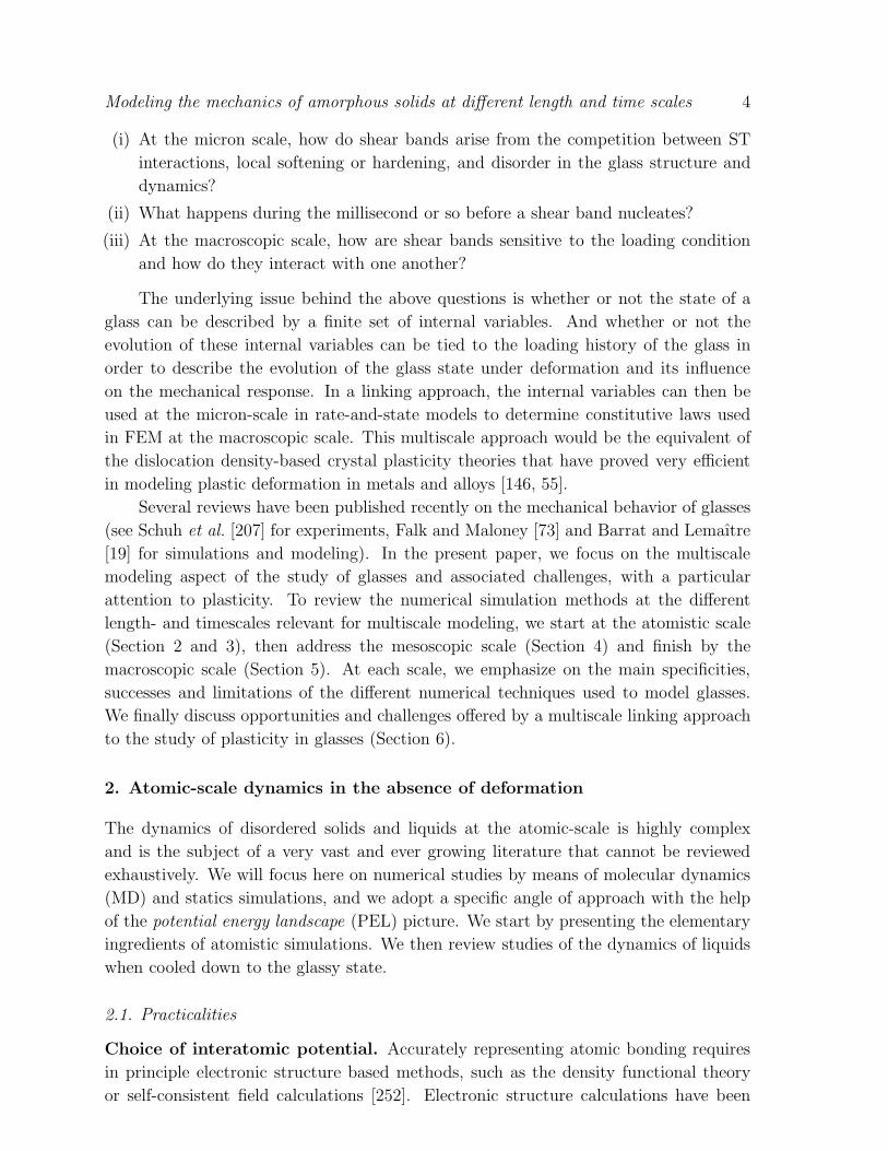
(i) At the micron scale, how do shear bands arise from the competition between ST
interactions, local softening or hardening, and disorder in the glass structure and
dynamics?
(ii) What happens during the millisecond or so before a shear band nucleates?
(iii) At the macroscopic scale, how are shear bands sensitive to the loading condition
and how do they interact with one another?
The underlying issue behind the above questions is whether or not the state of a
glass can be described by a finite set of internal variables. And whether or not the
evolution of these internal variables can be tied to the loading history of the glass in
order to describe the evolution of the glass state under deformation and its influence
on the mechanical response. In a linking approach, the internal variables can then be
used at the micron-scale in rate-and-state models to determine constitutive laws used
in FEM at the macroscopic scale. This multiscale approach would be the equivalent of
the dislocation density-based crystal plasticity theories that have proved very efficient
in modeling plastic deformation in metals and alloys [146, 55].
Several reviews have been published recently on the mechanical behavior of glasses
(see Schuh et al. [207] for experiments, Falk and Maloney [73] and Barrat and Lemaıtre
[19] for simulations and modeling). In the present paper, we focus on the multiscale
modeling aspect of the study of glasses and associated challenges, with a particular
attention to plasticity. To review the numerical simulation methods at the different
length- and timescales relevant for multiscale modeling, we start at the atomistic scale
(Section 2 and 3), then address the mesoscopic scale (Section 4) and finish by the
macroscopic scale (Section 5). At each scale, we emphasize on the main specificities,
successes and limitations of the different numerical techniques used to model glasses.
We finally discuss opportunities and challenges offered by a multiscale linking approach
to the study of plasticity in glasses (Section 6).
2. Atomic-scale dynamics in the absence of deformation
The dynamics of disordered solids and liquids at the atomic-scale is highly complex
and is the subject of a very vast and ever growing literature that cannot be reviewed
exhaustively. We will focus here on numerical studies by means of molecular dynamics
(MD) and statics simulations, and we adopt a specific angle of approach with the help
of the potential energy landscape (PEL) picture. We start by presenting the elementary
ingredients of atomistic simulations. We then review studies of the dynamics of liquids
when cooled down to the glassy state.
2.1. Practicalities
Choice of interatomic potential. Accurately representing atomic bonding requires
in principle electronic structure based methods, such as the density functional theory
or self-consistent field calculations [252]. Electronic structure calculations have been
Modeling the mechanics of amorphous solids at different length and time scales 5
applied to simulate liquids and glasses, but the tradeoff for increased accuracy is a
decrease in system size (a few hundred atoms) and in simulated time (a few picoseconds).
Monoatomic systems (for example [20, 108, 79]), silica glasses (for example [252, 105])
and metal alloys (for example [211, 80, 118, 86]) have been simulated but semi-empirical
potentials have also been used to access larger systems during longer times. For metallic
alloys for example, the embedded atom method (EAM) formalism has been employed,
in particular to model CuZr [63, 161, 160], CuZrAl [40] and CuMg [15] alloys. For
liquid and glassy silica and silicon, several empirical potentials have been adjusted in
order to fit, with a minimum number of parameters, ab-initio cohesive energy data
[20, 252] and experimental characteristics such as the melting temperature, short-range
order, diffusive motion, some characteristic vibrational frequencies and elastic moduli
[233, 247, 255, 21, 105, 101, 106, 34]. In the case of silicon, the difficulty is to find an
empirical potential able to describe the profound structural breakdown that occurs upon
melting, with an experimental average coordination of 4.0 in the solid phase (tetrahedral
order due to sp3 covalent bonding in the crystal as well as in the amorphous phase) and
of 6.4 in the liquid state [247]. Since the interatomic potentials depend on the full atomic
configuration, they can be decomposed into two-, three-body potentials and above. The
three-body potential serves to stabilize the ideal local bond angle, as in the famous
Stillinger-Weber empirical potential [233], expressed as:
V (1, ..., N) =∑
i<j
v2(i, j) +∑
i<j<k
v3(i, j, k) (1)
with
v2(i, j) = ǫ.A.(Br−pij − r−q
ij ) exp[(rij − a)−1], rij < a and =0 elsewhere (2)
and
v3(i, j, k) = h(rij, rik, θjik) + h(rji, rjk, θijk) + h(rki, rkj, θikj) (3)
with
h(rij, rik, θjik) = ǫλ exp[γ(rij − a)−1 + γ(rik − a)−1].(cos θjik +1
3)2, (4)
where rij is the bond length between atoms i and j and θijk is the angle between
the bonds ji and jk. The experimental pair correlation however is better reproduced
with more complex environment-dependent potentials, such as Tersoff potential [247] or
EDIP [21]. The latter is also able to represent the covalent-to-metallic transition through
a parameter depending on the local coordination and describing the angular stiffness
of the bond. These different empirical potentials have been tested on the nonlinear
mechanical response of samples submitted to a large shear [83] or crack propagation
[90]. In the case of silica, the ionic character of the bond is usually described through
a two-body potential with partial charges [255, 34, 162], while the covalent character
implies a three-body term [101]. Surprisingly enough, the local tetrahedral structure of
Si02 is well described by a simple two-body potential with different charges on Si and
O, even with a small cut-off of the interaction range [34].
Modeling the mechanics of amorphous solids at different length and time scales 6
ǫAA ǫBB ǫAB σAA σBB σAB RC CA CB TC
Kob-Andersen [122] 1 0.5 1.5 1 0.88 0.8 2.5 0.8 0.2 0.435
Wahnstrom [264] 1 1 1 1 5
6
11
122.5 0.5 0.5 0.57
Lancon et al. [129] 0.5 0.5 1 2 sin( π10) 2 sin(π
5) 1 5 0.45 0.55 0.485
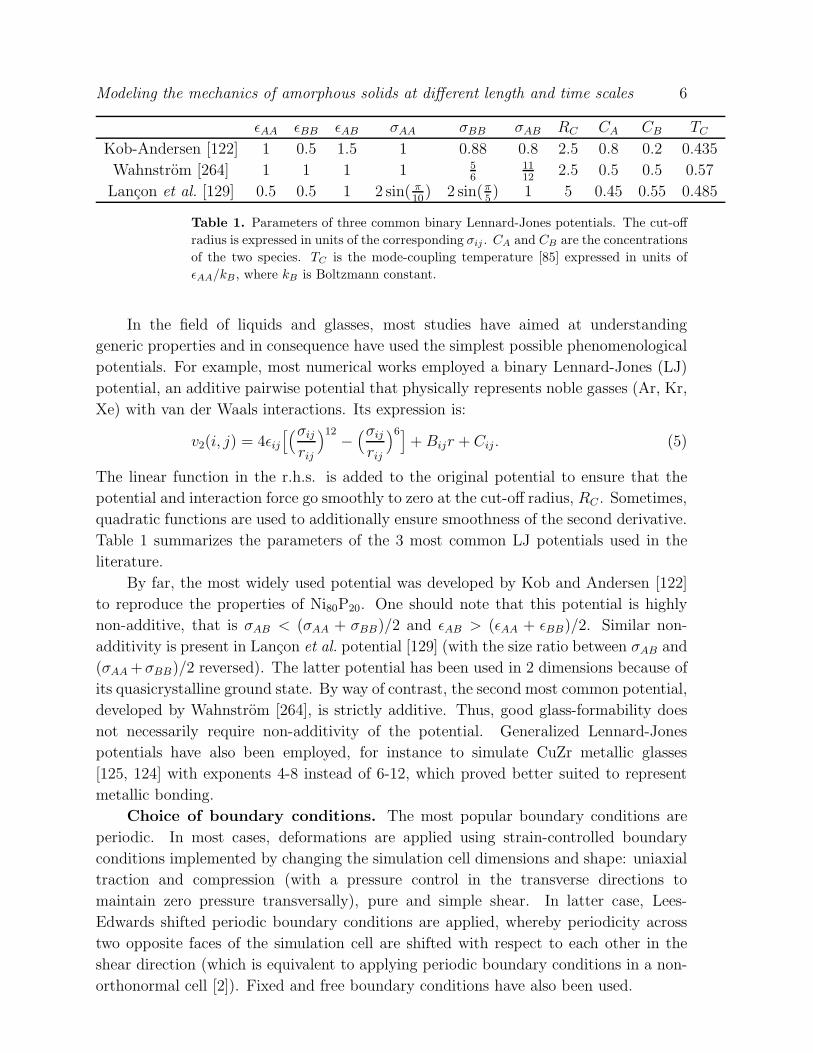
Table 1. Parameters of three common binary Lennard-Jones potentials. The cut-off
radius is expressed in units of the corresponding σij . CA and CB are the concentrations
of the two species. TC is the mode-coupling temperature [85] expressed in units of
ǫAA/kB, where kB is Boltzmann constant.
In the field of liquids and glasses, most studies have aimed at understanding
generic properties and in consequence have used the simplest possible phenomenological
potentials. For example, most numerical works employed a binary Lennard-Jones (LJ)
potential, an additive pairwise potential that physically represents noble gasses (Ar, Kr,
Xe) with van der Waals interactions. Its expression is:
v2(i, j) = 4ǫij[(σij
rij
)12
−(σij
rij
)6]
+Bijr + Cij . (5)
The linear function in the r.h.s. is added to the original potential to ensure that the
potential and interaction force go smoothly to zero at the cut-off radius, RC . Sometimes,
quadratic functions are used to additionally ensure smoothness of the second derivative.
Table 1 summarizes the parameters of the 3 most common LJ potentials used in the
literature.
By far, the most widely used potential was developed by Kob and Andersen [122]
to reproduce the properties of Ni80P20. One should note that this potential is highly
non-additive, that is σAB < (σAA + σBB)/2 and ǫAB > (ǫAA + ǫBB)/2. Similar non-
additivity is present in Lancon et al. potential [129] (with the size ratio between σAB and
(σAA+σBB)/2 reversed). The latter potential has been used in 2 dimensions because of
its quasicrystalline ground state. By way of contrast, the second most common potential,
developed by Wahnstrom [264], is strictly additive. Thus, good glass-formability does
not necessarily require non-additivity of the potential. Generalized Lennard-Jones
potentials have also been employed, for instance to simulate CuZr metallic glasses
[125, 124] with exponents 4-8 instead of 6-12, which proved better suited to represent
metallic bonding.
Choice of boundary conditions. The most popular boundary conditions are
periodic. In most cases, deformations are applied using strain-controlled boundary
conditions implemented by changing the simulation cell dimensions and shape: uniaxial
traction and compression (with a pressure control in the transverse directions to
maintain zero pressure transversally), pure and simple shear. In latter case, Lees-
Edwards shifted periodic boundary conditions are applied, whereby periodicity across
two opposite faces of the simulation cell are shifted with respect to each other in the
shear direction (which is equivalent to applying periodic boundary conditions in a non-
orthonormal cell [2]). Fixed and free boundary conditions have also been used.
Modeling the mechanics of amorphous solids at different length and time scales 7
The choice of boundary conditions is not inconsequential since fixed boundaries
favor localization of the deformation in simple shear [261]. Similarly, uniaxial traction
with free surfaces in the transverse directions also favor shear localization compared to
simple shear with periodic boundary conditions [39].
Molecular dynamics versus quasistatic simulations. The first step of an
atomistic simulation of a glass is to produce an initial configuration by quenching
a liquid using MD. The procedure involves first equilibrating the liquid at an
elevated temperature (typically several 1000 K) and then progressively decreasing the
temperature below the glass transition at either fixed volume or fixed pressure. The main
limitation of MD simulations is that the timescale is very limited, typically a few tens
of nanoseconds. As a consequence, MD quench rates are on the order of 1000 K/10−8 s,
i.e. 1010 to 1012 K/s, which is enormously high compared to experimental quench rates
that are rather on the order of 106 K/s for the first synthesized metallic glasses [121] to
0.1 K/s for the most recent bulk metallic glasses [111]. As a result, simulated glasses
are inevitably far less relaxed than experimental glasses, with consequences on their
propensity to form shear bands that will become apparent later in the text. Also, when
simulating the deformation of glasses using MD, one wishes to reach a strain of order 1
in the timescale of the simulation, resulting in typical strain rates of γ = 1/10−8 = 108
s−1 compared to typically 10−3 s−1 experimentally. In order to avoid this discrepancy,
one option is to apply quasistatic (QS) deformations [147, 151, 152]. The system is then
sheared in small increments followed by energy minimizations at fixed applied strain.
This protocol corresponds to the limit T → 0, since the energy minimizations remove
all thermal activation, and γ → 0, since the system is allowed to fully relax to a new
energy minimum before a new strain increment is applied [147].
The physical situation associated with the QS procedure involves two timescales
characteristic of the dynamics of glassy materials [25]. The first timescale, τdiss, is
the time it takes for a localized energy input to spread over the whole system and be
dissipated as heat. The corresponding mechanisms can be viscous (in a soft material)
or associated with phonon propagation or electron transfers (in a metallic glass). QS
deformation corresponds to a typical time between consecutive strain increments much
larger than τdiss, that is γ ≪ δγ/τdiss, where δγ is the elementary strain increment.
A second, much longer timescale is the structural relaxation time of the system, τα,
associated with spontaneous aging processes that take place at finite temperature in
the absence of external drive. By quenching after every displacement step, any such
processes are suppressed and the time elapsed between consecutive increments is thus
far smaller than τα, i.e. γ ≫ δγ/τα. Here, δγ, the elementary strain step, is chosen small
enough to ensure that the system remains in its initial basin when starting from any
equilibrium configuration (δγ depends on the system size, probably logarithmically [137]
and is on the order of 10−5 for L = 100 in LJ units in 2 and 3 dimensions [138]). This
picture is of course oversimplified. Relaxations in glasses are in general stretched [25],
meaning that relaxation processes take place over a broad spectrum of timescales and
the QS approach ignores the fast wing of the relaxation spectrum. Another drawback of
Modeling the mechanics of amorphous solids at different length and time scales 8
the QS approach is that it ignores thermal effects that are unavoidable in experiments.
The coupling between temperature and strain rate is highly non-trivial and progress in
this area is discussed in Section 3.2. The first steps towards using accelerated dynamics
have been taken [126, 194] in order to access slow dynamics at the atomic scale, but such
simulations are difficult because of the complexity of the configurational paths available
to disordered systems.
2.2. Cooling a liquid
Understanding the glass transition and the associated dramatic slowing down and
increasing heterogeneity of the liquid dynamics is a topic of intense research (for reviews,
see for example [67, 50, 246, 96, 241, 24]). This field has greatly benefited from the
recognition that the dynamics of a cooling liquid is intimately related to the topography
of its underlying potential energy landscape [267].
What is the potential energy landscape? An atomic configuration is
represented in configuration space by its position vector, R3N , a 3N-dimensional vector
for a system of N particles in 3 dimensions. The potential energy of the system, V (R3N),
is then a 3N-dimensional surface, termed the potential energy landscape (PEL), in the
(3N+1)-dimensional space composed of configuration space and the energy axis [84, 265].
It is important to note that the PEL depends only on the interatomic potential and the
boundary conditions. Thus, for a given potential and given boundary conditions, all
configurations of a system, whether they are crystalline, amorphous or liquid, share the
same PEL; only the region of configuration space visited by the system depends on the
state of the system.
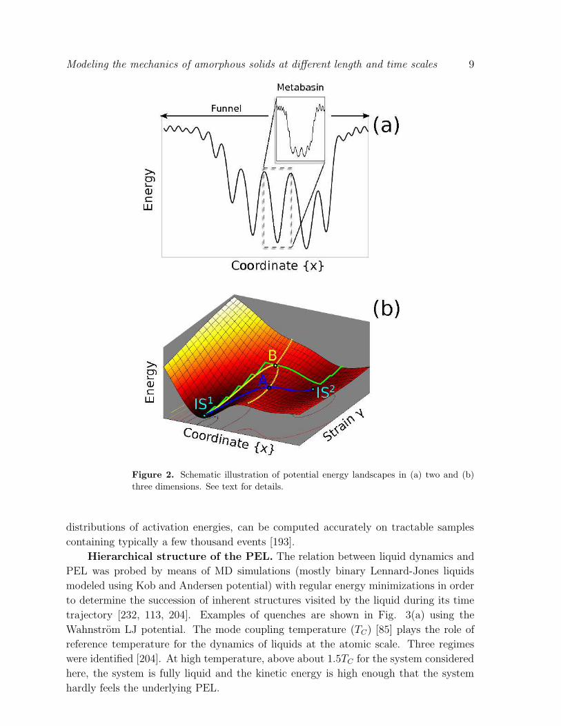
As sketched in Fig. 2 in two and three dimensions, the PEL contains extrema, or
stationary points, which may be local maxima, local minima called inherent structures
(IS) [232] (IS1 and IS2 in Fig. 2(b)) and saddle points (A in Fig. 2(b)). Stationary
points are classified by their index, which is the number of negative eigenvalues of the
Hessian matrix (matrix of second derivatives of the potential energy) computed at the
stationary point [265]. The PEL can be partitioned into valleys, or basins, that surround
each local minima [232, 231]. More precisely, the basin (of attraction) of an IS is the
region of configuration space where all configurations converge to the IS upon steepest-
descent energy minimization. In Fig. 2(b), the basins of IS1 and IS2 are delimited
by the yellow dashed line. Alternatively, the PEL can be partitioned using the basins
of attraction of all stationary points and not only local minima by minimizing the
objective function 1
2|∇V (R3N )|2 rather than the potential energy [6], although one has
to be careful because the objective function has more minima than stationary points on
the PEL [62].
The number of stationary points increases roughly as an exponential function of
the number of atoms in the system [232, 96]. It is therefore impossible in practice to list
exhaustively all stationary points in a PEL, except for very small systems (containing
typically 32 atoms or less [95, 7]). On the other hand, statistical information, such as
Modeling the mechanics of amorphous solids at different length and time scales 9
Figure 2. Schematic illustration of potential energy landscapes in (a) two and (b)
three dimensions. See text for details.
distributions of activation energies, can be computed accurately on tractable samples
containing typically a few thousand events [193].
Hierarchical structure of the PEL. The relation between liquid dynamics and
PEL was probed by means of MD simulations (mostly binary Lennard-Jones liquids
modeled using Kob and Andersen potential) with regular energy minimizations in order
to determine the succession of inherent structures visited by the liquid during its time
trajectory [232, 113, 204]. Examples of quenches are shown in Fig. 3(a) using the
Wahnstrom LJ potential. The mode coupling temperature (TC) [85] plays the role of
reference temperature for the dynamics of liquids at the atomic scale. Three regimes
were identified [204]. At high temperature, above about 1.5TC for the system considered
here, the system is fully liquid and the kinetic energy is high enough that the system
hardly feels the underlying PEL.
Modeling the mechanics of amorphous solids at different length and time scales 10
At lower temperatures, the system becomes supercooled and enters the so-called
landscape influenced regime. Between 1.5TC and TC , the liquid gets progressively
trapped in basins of decreasing energy, i.e. it remains for longer periods of time in
a given IS before hopping to the next IS with the help of thermal activation. A
decoupling develops between the rapid motion of the supercooled liquid inside a basin
(intrabasin vibration) and the infrequent transitions to a new basin (interbasin hoping)
[209]. Vibrations are however of large amplitude and the system spends most of its
time in the basins of attraction of saddle points, i.e. stationary points with index 1
and above [6, 28]. A well-defined relation was found between the average stationary
point index and the temperature or potential energy [6, 28] with the average index
vanishing precisely at TC . The progressive trapping of the system implies that the PEL
has a multifunnel structure [266, 265] where, as illustrated in Fig. 2(a), the basins are
organized in pockets of inherent structures with increasing energy barriers for decreasing
IS energy.
Funnels have a hierarchical structure. On short timescales, the system undergoes
a back and forth motion between a limited number of basins forming a cluster, also
called a metabasin [231], while on longer timescales, the system performs an irreversible
Brownian diffusion between metabasins [29, 58, 57, 54]. The above dynamics implies
that, as illustrated in Fig. 2(a), metabasins are composed of basins connected by
low-energy saddle points, while different metabasins are separated by higher energy
barriers. Moreover, some metabasins are visited quickly whereas others are very long-
lived [59]. The overall structure of the PEL is therefore a multifunnel rough landscape
[266] with a hierarchy of energy barriers connecting basins and metabasins. Trapping of
the supercooled liquid in this maze of interconnected basins and the multistep hopping
process between long-lived metabasins which dictates the slow dynamics was put forward
to explain the rapid slowing down and stretched exponential relaxations of liquids across
the glass transition [59, 96].
Below TC , the system enters the glassy state, or landscape dominated regime
[205], which is the true thermally-activated regime where the system spends most time
vibrating near local minima and undergoes rare and thermally-activated transitions
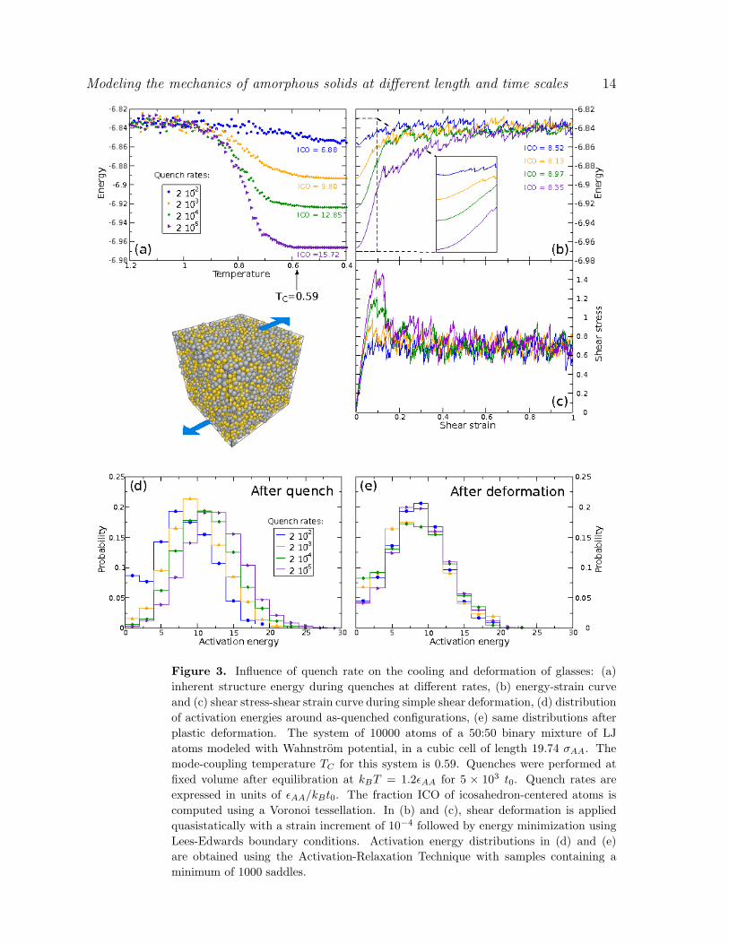
between ISs. As seen in Fig. 3(a), the energy of the final inherent structure decreases
with decreasing quench rate, meaning that the glass is better relaxed. This is a
consequence of the funnel structure of the PEL where decreasing quench rates give more
time to the system to explore lower regions of the funnel before being trapped. When the
temperature is lowered below TC , the waiting time between transitions exceeds rapidly
MD timescales and the PEL can no longer be probed by direct MD simulations. In this
regime, saddle-point search methods can be used to identify activated states on a PEL.
Examples of distributions of the activation energies of transition states (saddle-points
of index 1) around the final ISs obtained after the above quenches are shown in Fig.
3(d). These distributions were obtained using the activation-relaxation technique (ART)
[149, 33, 194]. Distributions of activation energies have a characteristic shape with a
broad energy spectrum and a maximum, i.e. a most likely activation energy. Similar
Modeling the mechanics of amorphous solids at different length and time scales 11
distributions were obtained in LJ glasses [6, 164, 194] as well as amorphous silicon
[254]. Their exponential tail agrees with the master-equation approach developed by
Dyre [66] in the case of rapidly quenched glasses. Also, the density of low activation
saddles (below typically 5ǫAA for this system) decreases for configurations relaxed more
slowly. The latter configurations are therefore more stable, both thermodynamically,
because they have a lower energy, and kinetically, because they are surrounded by higher
activation energies. In experimental glasses that are quenched much more slowly than in
simulations, we expect activation energies to be shifted towards higher energies without
low activation energies, although a quantitative study of this dependence remains to be
done.
Below TC , glasses are not in thermal equilibrium but keep evolving towards deeper
regions of the PEL. This relaxation process is slow and referred to as structural
relaxation or physical aging [253]. Two relaxation timescales have been identified, β-
relaxations on short timescales and α-relaxations on longer timescales [110]. In relation
with the PEL picture, Stillinger [231] hypothesized that β-relaxations are transitions
inside a given metabasin while α-relaxations would be transitions between metabasins.
MD simulations confirmed the first hypothesis but showed that the second is only partly
true. A β-relaxation is a transition inside a given metabasin, termed nondiffusive by
Middleton and Wales [164] because it corresponds to a slight repositioning of atoms
inside their shell of nearest neighbors (cage effect). By way of contrast, transitions
between metabasins involve bond switching and correspond to localized rearrangements
in the form of string-like sequences of displacements whose size (∼ 10 atoms) increases
as the temperature decreases towards TC [123, 60, 61, 205, 230]. One such dynamical
heterogeneity is however not an α-relaxation in itself because it occurs on a timescale of
the order of 1/10 to 1/5 of the α-relaxation timescale [8]. An α-relaxation is therefore
made of 5 to 10 metabasin transitions. It remains localized in the microstructure but
involves more atoms than string-like events (∼ 40 atoms), is more globular and was
termed democratic [8]. Dynamical heterogeneities have been shown correlated to both
localized soft modes [268] and fluctuations of static structural order [117, 241].
Atomic-scale glass structure. Although glasses are disordered at long range,
they exhibit short and medium range orders. There exists no general theory to predict
the packing in a given glass but short and medium range orders have been studied in
a number of metallic glasses using a combination of experiments and simulations (see
for example Refs. [124, 63, 211, 38, 179, 88]). It was shown that solute atoms tend
to remain separated from one another and their shell of first neighbors tends to form
simple polyhedra. In several binary glasses, and in particular CuZr metallic glasses,
the most abundant polyhedra are Cu-centered icosahedra, therefore atoms with a local
fivefold atomic environment [113, 39, 182]. Moreover, it was shown that in this system,
the short-range order can be characterized by the density of these icosahedra, which
density is strongly correlated with the level of relaxation of the glass. In particular,
Cheng et al. [39] showed that the density of Cu-centered icosahedra increases rapidly
in the landscape influenced regime and reaches a low-temperature value that increases
Modeling the mechanics of amorphous solids at different length and time scales 12
with decreasing quench rate, i.e. increasing levels of relaxation. It is known that with
the Wahnstrom LJ potential used in Fig. 3(a), icosahedron-centered atoms characterize
the short-range order [42, 180]. We computed their fraction, noted ICO in Fig. 3(a),
and found that the fraction of icosahedron-centered atoms increases with decreasing
quench rate, which confirms the result mentioned above: the short-range order in glasses
increases with decreasing quench rates. Icosahedron-centered atoms are clear markers
of the level of relaxation of a glass but they concern unfortunately only a certain class
of metallic glasses. For instance, they are not the most frequent local environment in
monoatomic glasses and the addition of a three-body term to the interatomic potential
changes drastically its atomic structure and ability to crystallize [168, 240, 218, 78].
3. Atomic-scale deformation of glasses
3.1. Quasi-static deformation
PEL and QS deformation. The PEL picture also proved useful to rationalize the
behavior of glasses under deformation, as first demonstrated by Malandro and Lacks
[147, 148, 127]. The picture is clearest during QS deformation where the glass evolution
is exclusively strain activated and when rigid boundary conditions are used. In this case,
a shear strain is applied by rigidly moving in opposite directions two slabs of atoms on
opposite faces of the simulation cell. The PEL is then unchanged because the potential
energy function is unchanged (the situation is different when stresses are applied because
the PEL is then tilted by the work of the applied stress [14]). The effect of an applied
strain is then to force the system to visit new regions of the PEL. More precisely,
adding a strain increment to a simulation cell amounts to moving the system in a given
direction of configuration space, which we call the strain vector γ. The PEL may thus
be represented in three dimensions as in Fig. 2(b), with the strain vector γ decoupled
from the other dimensions of configuration space, noted x. A possible path during
QS deformation is shown in green in Fig. 2(b). Initially, the as-quenched glass is in an
inherent structure, noted IS1, at the bottom of an energy basin. The strain increments
push the system away from this initial configuration. After each strain increment, the
energy is minimized at fixed strain, i.e. minimized in the hyperplane perpendicular
to the strain vector. The system then relaxes to the nearest local minimum in the
hyperplane, which lies on the branch of stable equilibrium at the bottom of the basin,
shown as a yellow solid line in Fig. 2(b). During the first few strain increments, the
system remains in the initial basin and the deformation is purely elastic and reversible;
if the strain is removed, the system relaxes back along the stable branch down to IS1.
The extension of this region of strict reversibility increases with decreasing system size
and increasing level of relaxation of the quenched glass (see Fig. 3(b)).
With increasing strain, the system reaches the edge of the initial basin, noted
B in Fig. 2(b), a position of instability on the PEL where the stable branch at the
bottom of the basin (yellow solid line) meets the unstable branch on the border of the
Modeling the mechanics of amorphous solids at different length and time scales 13
basin (yellow dashed line). At this point, one eigenvalue of the Hessian matrix in the
hyperplane of constant strain vanishes. Such instability is called a saddle-node or a fold
bifurcation [87]. Near the instability, glasses have a universal behavior [151, 37, 115]:
the vanishing eigenvalue and energy barrier between stable and unstable positions go to
zero as (γC−γ)1/2 and (γC−γ)3/2 respectively, where γC is the strain at the bifurcation.
The subsequent energy minimization takes the system into a new basin, centered on IS2
in Fig. 2(b). During the relaxation, the system is out-of-equilibrium and its trajectory
depends on the energy minimization algorithm used. Across the transition, the position
of the system on the PEL, as well as its energy and stress are discontinuous. The
transition is irreversible because if the strain is decreased, the system remains in the
new basin. Such transitions are the elementary events that produce dissipation and
plastic strain during the deformation process. During a QS process the kinetic energy
produced by the elementary events is assumed to be very efficiently dissipated in order
to relax in the next visited basin.
Shear transformations and avalanches. Fig. 3(b) and (c) show examples of
energy-strain and stress-strain curves during simple shear deformation of the quenched
glasses obtained in Fig. 3(a). As expected from the above discussion, the curves are
made of continuous elastic segments intersected by plastic events where stress and energy
are discontinuous [147, 148, 151, 244]. The deformation starts with a regime where
the stress increases linearly with strain and the energy increases quadratically. This
regime is larger than the region of strict reversibility mentioned above and contains small
plastic events as evidenced by the discontinuities in the inset of Fig. 3(b). The latter
correspond to localized rearrangements in the microstructure [148, 151, 244, 159, 51].
They are the shear transformations (STs) proposed by Argon [10, 11] as elementary
plastic events in amorphous solids. An example in two dimensions is shown in Fig.
1(a). The rearrangement is composed of two regions: a plastic core region where atomic
bonds are cut and reformed and a surrounding elastic region, which responds elastically
to the plastic rearrangement. In Fig. 1(a), mainly the elastic field is visible with a
quadrupolar symmetry [151, 244], characteristic of an Eshelby field (see Section 4.1 and
Eq. 20). This field was shown to scale with the eigenmode whose eigenvalue vanishes at
the instability [150, 135, 245]. Evaluating the size of a ST requires separating the plastic
region, which is the true ST zone, from the elastic surrounding. Such separation is not
straightforward, but usual estimates are 20 atoms in two dimensions [244] and 100 in
three dimensions [276]. The corresponding local strain is about 0.1, which satisfies the
Lindemann instability criterion with a relative displacement of the particles of a tenth
of the interatomic distance [244, 250].
As strain increases, the system reaches its true elastic limit where plastic flow
starts. Irreversible events are then dominated by large rearrangements that span the
entire simulation cell [151, 244, 16]. Careful analysis of energy minimizations during
such rearrangements [151, 53] showed that, although the system is out-of-equilibrium
and does not cross any equilibrium configuration (otherwise the energy minimization
would stop), the path can be decomposed into a succession of localized unstable STs
Modeling the mechanics of amorphous solids at different length and time scales 14
Figure 3. Influence of quench rate on the cooling and deformation of glasses: (a)
inherent structure energy during quenches at different rates, (b) energy-strain curve
and (c) shear stress-shear strain curve during simple shear deformation, (d) distribution
of activation energies around as-quenched configurations, (e) same distributions after
plastic deformation. The system of 10000 atoms of a 50:50 binary mixture of LJ
atoms modeled with Wahnstrom potential, in a cubic cell of length 19.74 σAA. The
mode-coupling temperature TC for this system is 0.59. Quenches were performed at
fixed volume after equilibration at kBT = 1.2ǫAA for 5 × 10³ t0. Quench rates are
expressed in units of ǫAA/kBt0. The fraction ICO of icosahedron-centered atoms is
computed using a Voronoi tessellation. In (b) and (c), shear deformation is applied
quasistatically with a strain increment of 10−4 followed by energy minimization using
Lees-Edwards boundary conditions. Activation energy distributions in (d) and (e)
are obtained using the Activation-Relaxation Technique with samples containing a
minimum of 1000 saddles.
Modeling the mechanics of amorphous solids at different length and time scales 15
that trigger each other through their elastic strain and stress fields. The latter thus play
the role in QS simulations of a mechanical noise that can push local regions beyond their
stability limit leading to out-of-equilibrium cascades of STs [135]. Avalanches do not
necessarily lead to persistent shear bands since, as discussed below, depending on the
boundary conditions and on the interatomic interactions, the cumulated deformation
can remain homogeneous in the avalanche regime for several 100 % strain.
Relating the elastic limit to the PEL picture, Harmon et al. [89] proposed that the
elastic limit occurs when the glass leaves its initial metabasin while STs are transitions
between basins inside a given metabasin. However, from the PEL analysis of supercooled
liquids presented in Section 2.2, we know that transitions inside a given metabasin
correspond to small atomic adjustments that retain the nearest-neighbor shell while
transitions between metabasins involve bond switching, as in STs. STs are thus
elementary transitions between metabasins and are analogous to string-like events in
supercooled liquids, while avalanches, made of a succession of STs, correspond to a
transition over several metabasins and would be analogous to α-relaxations.
A question of prime importance then arises: can we predict the location of the next
ST? Or said differently, is there a structural signature that indicates a region prone
to plastic rearrangements, also called weak region, or shear transformation zone [72]?
Historically, the first proposed criterion was based on local atomic stresses. Srolovitz
et al. [226, 227] in their early simulations of metallic glass plasticity identified three
types of structural defects: atoms with high atomic tensile or compressive stress (n-
and p-type defects respectively) and atoms with high atomic shear stress (τ -defects).
Plastic rearrangements were shown uncorrelated with n- and p-defects but a correlation
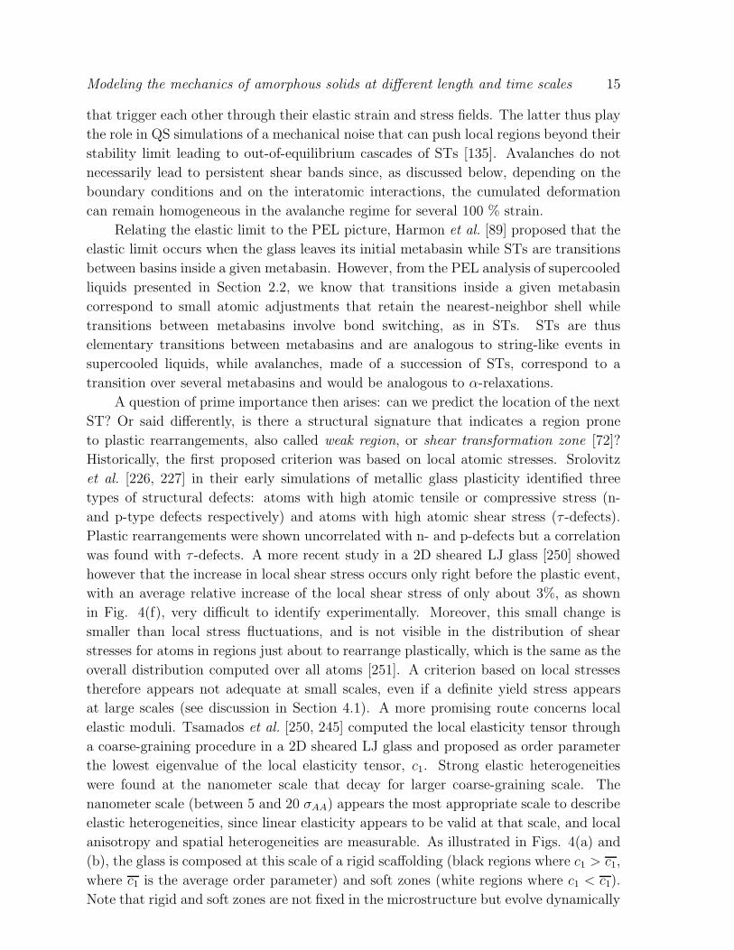
was found with τ -defects. A more recent study in a 2D sheared LJ glass [250] showed
however that the increase in local shear stress occurs only right before the plastic event,
with an average relative increase of the local shear stress of only about 3%, as shown
in Fig. 4(f), very difficult to identify experimentally. Moreover, this small change is
smaller than local stress fluctuations, and is not visible in the distribution of shear
stresses for atoms in regions just about to rearrange plastically, which is the same as the
overall distribution computed over all atoms [251]. A criterion based on local stresses
therefore appears not adequate at small scales, even if a definite yield stress appears
at large scales (see discussion in Section 4.1). A more promising route concerns local
elastic moduli. Tsamados et al. [250, 245] computed the local elasticity tensor through
a coarse-graining procedure in a 2D sheared LJ glass and proposed as order parameter
the lowest eigenvalue of the local elasticity tensor, c1. Strong elastic heterogeneities
were found at the nanometer scale that decay for larger coarse-graining scale. The
nanometer scale (between 5 and 20 σAA) appears the most appropriate scale to describe
elastic heterogeneities, since linear elasticity appears to be valid at that scale, and local
anisotropy and spatial heterogeneities are measurable. As illustrated in Figs. 4(a) and
(b), the glass is composed at this scale of a rigid scaffolding (black regions where c1 > c1,
where c1 is the average order parameter) and soft zones (white regions where c1 < c1).
Note that rigid and soft zones are not fixed in the microstructure but evolve dynamically
Modeling the mechanics of amorphous solids at different length and time scales 16
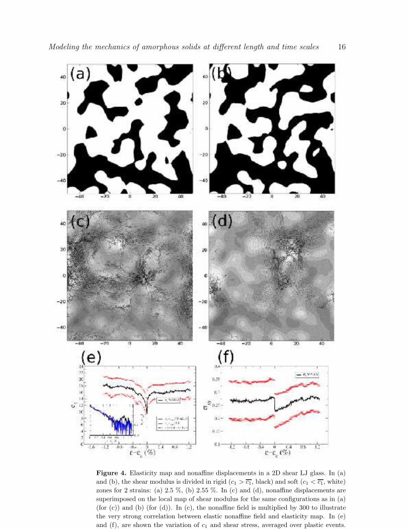
Figure 4. Elasticity map and nonaffine displacements in a 2D shear LJ glass. In (a)
and (b), the shear modulus is divided in rigid (c1 > c1, black) and soft (c1 < c1, white)
zones for 2 strains: (a) 2.5 %, (b) 2.55 %. In (c) and (d), nonaffine displacements are
superimposed on the local map of shear modulus for the same configurations as in (a)
(for (c)) and (b) (for (d)). In (c), the nonaffine field is multiplied by 300 to illustrate
the very strong correlation between elastic nonaffine field and elasticity map. In (e)
and (f), are shown the variation of c1 and shear stress, averaged over plastic events.

Modeling the mechanics of amorphous solids at different length and time scales 17
during the deformation (as seen by comparing Figs. 4(a) and (b)). Also, as shown in
Figs. 4(c) and (d), a strong correlation was found between plastic activity and soft
zones at the nanometer scale: c1 vanishes locally prior to a plastic event, with a marked
37% exponential decay of its amplitude, over a characteristic strain range of 0.2%.
Elastic constants being related to the Hessian matrix, this result shows that the global
Hessian matrix, which has a vanishing eigenvalue at the plastic event, can be computed
locally over finite-size regions with the same property: the local Hessian matrix has a
vanishing eigenvalue in the region of plastic activity. But noticeably, the decay of the
heterogeneous elastic constants measured on the local Hessian matrix [250], that is at
the nanometer scale, appears far before (δγ ≈ 0.2%) the decay of the eigenvalues of the
global Hessian (which occurs only within 10−3% of the transition [150] with possibly
an influence of the simulation cell size). Prediction of plastic activity thus combines
the local measurement (at the nanometer scale) of a global quantity (the coefficients
of the Hessian matrix). The same result was obtained for dislocation nucleation in
crystals [166]. However, as shown in Fig. 4(e), c1 decreases only near the instability
and the next plastic event cannot be predicted until the glass is brought close to the
instability. The question of the existence of identifiable structural defects in metallic
glasses is therefore still largely open. The situation is different in amorphous silicon
where weak (or liquidlike) and strong (solidlike) regions can be identified by looking at
their radial and angular distribution functions [52, 240, 78].
Influence of initial configuration. As seen in Figs. 3(b) and (c), plastic yielding
strongly depends on the level of relaxation of the initial glass. Slowly quenched glasses
that are more relaxed show a marked upper yield point followed by softening, while less
relaxed glasses have no upper yield point [253, 213, 215, 40, 78]. Also, the extension
of the purely elastic regime increases strongly with the level of relaxation of the glass.
After yielding, when simple shear is applied as in Fig. 3, the glass enters a steady state
regime, called a flow state, which is independent of the initial configuration in the sense
that the energy, stress and fraction of icosahedron-centered atoms reach steady state
values independent of the initial configuration, as shown in Fig. 3(b). One may say that
the glass has lost the memory of its initial configuration [253]. Persistent localization
has been observed in this regime, but depends on the level of relaxation of the initial
quenched glass, the boundary conditions as well as the interatomic potential. Persistent
localization occurs only in slowly quenched glasses [213] and is favored in simple shear
by fixed boundaries [261] and in uniaxial straining by free surfaces [213, 215, 40, 39]. A
strong three-body term in the interatomic potential also favors plastic localization, as
well as a low pressure [240, 78]. Sampling of the PEL around deformed configurations
taken from the flow state, as shown in Fig. 3(e), shows a marked increase in the density
of low activation energies compared to the initial quenched glasses except for the most
rapidly quenched glass [193, 194]. This effect has also been measured experimentally
[120]. Similarly, as seen in Fig. 3(b), the fraction of icosahedron-centered atoms
decreases after deformation [39], again with the exception of the most rapidly quenched
glass, which was so far from equilibrium initially that it evolved towards a slightly more
Modeling the mechanics of amorphous solids at different length and time scales 18
relaxed glass during deformation, a process called overaging [263].
3.2. Influence of temperature
Deformation acts in a way analogous to heating above TC since it accelerates the
dynamics of the glass and gives access to high-energy ISs that had become inaccessible
below TC . The glass microstructure evolution under deformation, or rejuvenation [253],
has been opposed to aging because the deformation reverses the aging process by
increasing the energy of the glass and decreasing its stability. Also, as seen in Fig.
3(b), the steady-state IS energy in deformation is the same as in the high-temperature
liquid regime. Moreover, it is known experimentally that the thermal history (annealing)
affects the structure of a glass through its density fluctuations at rest [142, 49]. This
effect could be compared with the structural changes that occur when the system is
submitted to a plastic deformation at a given strain rate. In addition, the plateau
resulting from the cage effect [22], which arises in temporal correlation functions used
to characterize the dynamics of glasses, disappears progressively with both an increasing
shear rate and an increasing temperature. Finally, it is well-known experimentally that
the viscosity of a supercooled metallic liquid [163, 190, 116] or of oxide glasses [220]
decreases as a function of both temperature or shear rate. There is therefore a strong
interplay between temperature and strain rate. From a theoretical point of view, the
effect of temperature has mainly been taken into account up to now in mean-field models
of plasticity, where plastic events are triggered randomly by thermal fluctuations in
specific distributions of energy barriers [224, 92, 223] or activated volumes [72]. In the
numerical simulation of mechanically deformed systems at finite temperature, two main
difficulties must be considered: first the competition between the mechanically driven
dynamics and the local dynamics of the thermostat used to maintain the temperature,
and second the necessity to identify very carefully the temperature domain studied,
which is a function of the applied shear rate.
Influence of the thermostat. This first difficulty is inherent to all MD
simulations. The latter consist of solving the discretized Newton’s equations of motion
with different constraints, such as constant total energy (microcanonical ensemble)
or constant temperature (canonical ensemble). The temperature is defined by the
equipartition theorem through the average fluctuation of particle velocities:
〈N∑
i=1
1
2miδv
2
i 〉 =3
2NkBT. (6)
When a system is deformed plastically by MD, a thermostat must be used
because the work produced by the plastic deformation is transformed into heat and the
temperature will rise indefinitely. Interestingly, all thermostats involve characteristic
timescales that depend on arbitrary parameters. For example, the simplest thermostats
(Berendsen thermostat, rescaling of velocities) [77] preserve Eq. with a characteristic
time depending on the coupling coefficient to the heat bath for Berendsen thermostat
and the frequency of rescaling for the velocity rescaling. More elaborated thermostats,
Modeling the mechanics of amorphous solids at different length and time scales 19
Individual Particle
−4.0 −2.0 0.0 2.0 4.0
X non−affine
−0.5
0.0
0.5
1.0
Ynon−affine
(a)
0.0 20.0 40.0 60.0−50.0
0.0
50.0
X nonaffine
Y n
onaffi
ne
X
Y
(b)
(c) (d)
Particles
Van HoveElastic Plastic
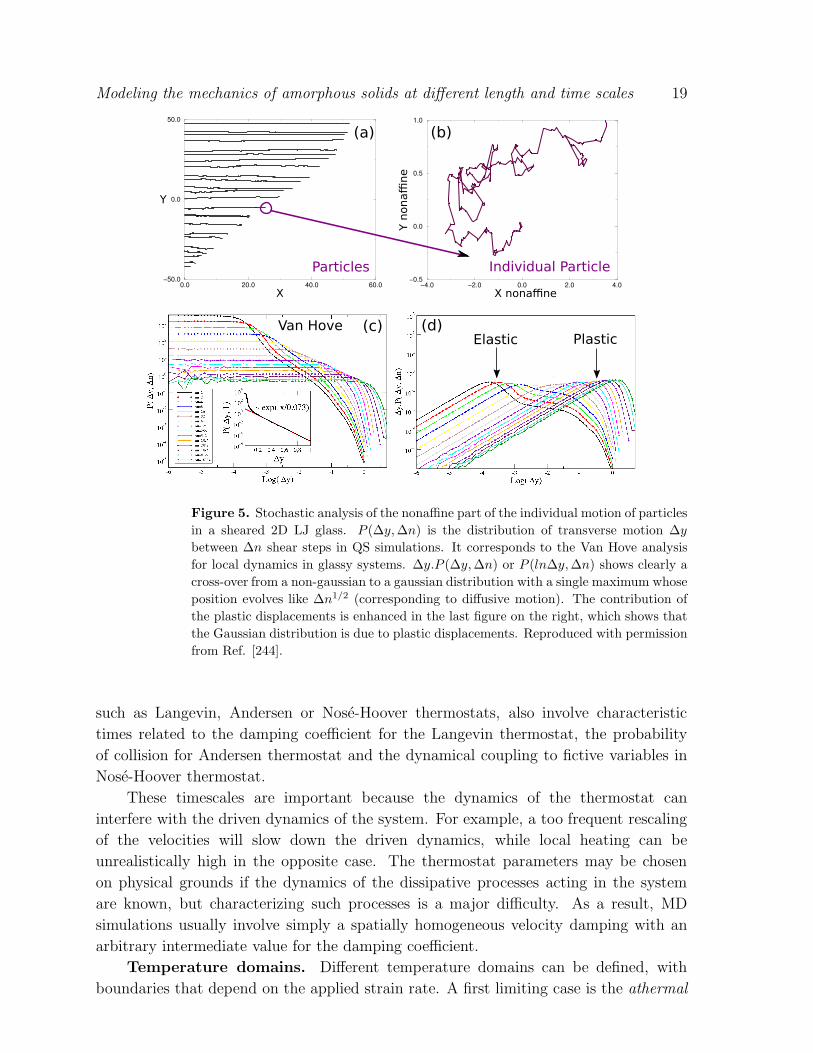
Figure 5. Stochastic analysis of the nonaffine part of the individual motion of particles
in a sheared 2D LJ glass. P (∆y,∆n) is the distribution of transverse motion ∆y
between ∆n shear steps in QS simulations. It corresponds to the Van Hove analysis
for local dynamics in glassy systems. ∆y.P (∆y,∆n) or P (ln∆y,∆n) shows clearly a
cross-over from a non-gaussian to a gaussian distribution with a single maximum whose
position evolves like ∆n1/2 (corresponding to diffusive motion). The contribution of
the plastic displacements is enhanced in the last figure on the right, which shows that
the Gaussian distribution is due to plastic displacements. Reproduced with permission
from Ref. [244].
such as Langevin, Andersen or Nose-Hoover thermostats, also involve characteristic
times related to the damping coefficient for the Langevin thermostat, the probability
of collision for Andersen thermostat and the dynamical coupling to fictive variables in
Nose-Hoover thermostat.
These timescales are important because the dynamics of the thermostat can
interfere with the driven dynamics of the system. For example, a too frequent rescaling
of the velocities will slow down the driven dynamics, while local heating can be
unrealistically high in the opposite case. The thermostat parameters may be chosen
on physical grounds if the dynamics of the dissipative processes acting in the system
are known, but characterizing such processes is a major difficulty. As a result, MD
simulations usually involve simply a spatially homogeneous velocity damping with an
arbitrary intermediate value for the damping coefficient.
Temperature domains. Different temperature domains can be defined, with
boundaries that depend on the applied strain rate. A first limiting case is the athermal
Modeling the mechanics of amorphous solids at different length and time scales 20
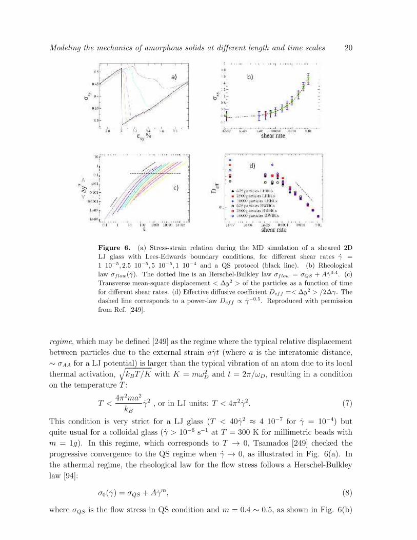
Figure 6. (a) Stress-strain relation during the MD simulation of a sheared 2D
LJ glass with Lees-Edwards boundary conditions, for different shear rates γ =
1 10−5, 2.5 10−5, 5 10−5, 1 10−4 and a QS protocol (black line). (b) Rheological
law σflow(γ). The dotted line is an Herschel-Bulkley law σflow = σQS + Aγ0.4. (c)
Transverse mean-square displacement < ∆y2 > of the particles as a function of time
for different shear rates. (d) Effective diffusive coefficient Deff =< ∆y2 > /2∆γ. The
dashed line corresponds to a power-law Deff ∝ γ−0.5. Reproduced with permission
from Ref. [249].
regime, which may be defined [249] as the regime where the typical relative displacement
between particles due to the external strain aγt (where a is the interatomic distance,
∼ σAA for a LJ potential) is larger than the typical vibration of an atom due to its local
thermal activation,√
kBT/K with K = mω2
D and t = 2π/ωD, resulting in a condition
on the temperature T :
T <4π2ma2
kBγ2 , or in LJ units: T < 4π2γ2. (7)
This condition is very strict for a LJ glass (T < 40γ2 ≈ 4 10−7 for γ = 10−4) but
quite usual for a colloidal glass (γ > 10−6 s−1 at T = 300 K for millimetric beads with
m = 1g). In this regime, which corresponds to T → 0, Tsamados [249] checked the
progressive convergence to the QS regime when γ → 0, as illustrated in Fig. 6(a). In
the athermal regime, the rheological law for the flow stress follows a Herschel-Bulkley
law [94]:
σ0(γ) = σQS + Aγm, (8)
where σQS is the flow stress in QS condition and m = 0.4 ∼ 0.5, as shown in Fig. 6(b)
Modeling the mechanics of amorphous solids at different length and time scales 21
[22, 196, 133, 249]. Similar behavior was also found experimentally in dense colloidal
systems [41, 242].
Under deformation at finite temperature, the particles exhibit a thermal as well
as a mechanically-driven diffusion. Collective effects in atomic diffusion in glasses have
been known for a long time [69]. In the QS regime, the particles display a diffusive
behavior at large strains due only to the plastic rearrangements upon external driving
[244, 136, 249] as shown in Fig. 5. In the athermal regime, the particles show first a
ballistic motion followed by a diffusive behavior at longer timescales (see Fig. 6 (d)) with
a cross-over time that decreases for increasing shear rates γ. Interestingly, as shown in
Fig. 6(d), in the 2D LJ glass studied in Ref. [249], the diffusive coefficient, Deff , defined
as a function of the strain γ rather than time (to transpose easily the definition to the
QS regime) decreases with the shear rate as Deff ≡ 〈∆y2〉/2∆γ ∝ γ−0.5 for large γ, with
a finite-size saturation at small γ, i.e. in the QS regime. This decrease of the diffusion
coefficient can be compared to the decrease of the Lindemann relaxation time tMSD
defined by < ∆y2(tMSD) >1/2= 0.1a, which corresponds to the typical time a particle
needs to escape definitely from its initial cage (here through the plastic rearrangements
due to the external driving) and is often associated with τα, the characteristic time for
α-relaxation (see Section 2.2). Of course, tMSD ∼ τα ∝ γ−0.5 due to the γ-dependence
of Deff . Also, the effective viscosity η follows Herschel-Bulkley law with approximately
the same strain-rate dependence η ≡ (σflow − σQS)/γ ∝ γ−m′
, with m′ = 0.5 ∼ 0.6
as deduced from Fig. 6(b). This is in agreement with a Maxwell-like interpretation
of the viscosity where τα = η/µ, µ being the shear modulus [43]. Tsamados [249]
proposed an interpretation of this dependence of the relaxation time with γ. The idea
is that the rheological behavior of the amorphous material results from the competition
between the propagation and nucleation of plastic rearrangements. The typical distance
between thermally-activated nucleated sites in a 2D system is dn = 1/(ρnγt)1/2 where
ρn is a density of nucleated sites per unit strain, depending probably on T . The typical
distance covered by mechanically-triggered plastic rearrangements due to the diffusion
of plastic activity [244, 217, 155] from a given site is dp = (Dpt)1/2. If we assimilate the
relaxation time to the time at which dn = dp, we obtain:
τα =1
√
ρnγDp
∝ γ−0.5, (9)
in agreement with the previous discussion.
In the well-defined athermal regime, the rheological law of the system is thus a
Herschel-Bulkley law (Eq. 8) and the dynamics is entirely due to the succession of
plastic rearrangements that enable to recover a diffusive memory-free behavior for the
particles. Note however that finite size effects are very important at small γ, i.e. in
the QS regime, and they disappear only for sufficiently large strain rates, typically
γ > 10−4 (see Fig. 6(d)). The diffusion coefficient then becomes a well-defined intensive
parameter, with a finite non-zero value even at very small temperatures.
In another study of the mechanical behavior of glassy materials at low temperature,
Modeling the mechanics of amorphous solids at different length and time scales 22
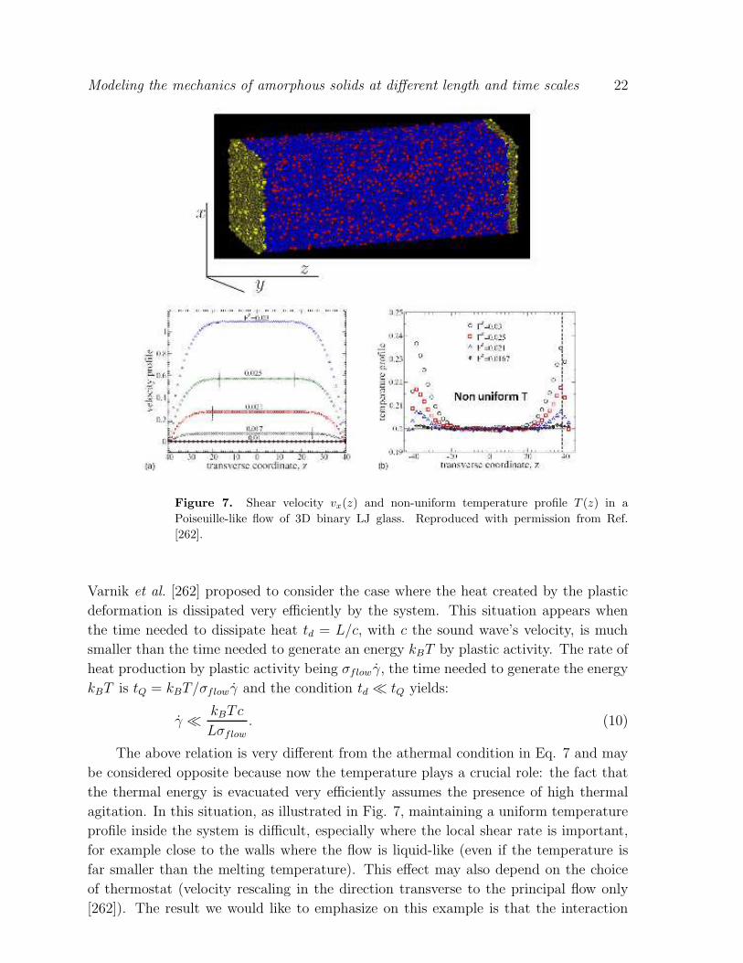
Figure 7. Shear velocity vx(z) and non-uniform temperature profile T (z) in a
Poiseuille-like flow of 3D binary LJ glass. Reproduced with permission from Ref.
[262].
Varnik et al. [262] proposed to consider the case where the heat created by the plastic
deformation is dissipated very efficiently by the system. This situation appears when
the time needed to dissipate heat td = L/c, with c the sound wave’s velocity, is much
smaller than the time needed to generate an energy kBT by plastic activity. The rate of
heat production by plastic activity being σflowγ, the time needed to generate the energy
kBT is tQ = kBT/σflowγ and the condition td ≪ tQ yields:
γ ≪kBTc
Lσflow. (10)
The above relation is very different from the athermal condition in Eq. 7 and may
be considered opposite because now the temperature plays a crucial role: the fact that
the thermal energy is evacuated very efficiently assumes the presence of high thermal
agitation. In this situation, as illustrated in Fig. 7, maintaining a uniform temperature
profile inside the system is difficult, especially where the local shear rate is important,
for example close to the walls where the flow is liquid-like (even if the temperature is
far smaller than the melting temperature). This effect may also depend on the choice
of thermostat (velocity rescaling in the direction transverse to the principal flow only
[262]). The result we would like to emphasize on this example is that the interaction
Modeling the mechanics of amorphous solids at different length and time scales 23
between the local temperature and local shear rate can affect the local dynamics and
that local temperature and local dynamics are strongly coupled as soon as we depart
from the athermal regime.
Indeed, identifying a single characteristic temperature for the rheological behavior
of driven amorphous solids is very difficult. By looking at the detailed statistics of
stress jumps in the stress-strain curve of a binary glass (with a Berendsen thermostat),
Karmakar et al. [115] identified two main characteristic temperatures and showed that
we can define separately cross-overs due to thermal fluctuations and strain rate. The
cross-over due to thermal fluctuations is obtained by comparing the energy dissipated
during plastic rearrangements 〈∆U〉/N to the thermal energy kBT . The finite-size
scaling of 〈∆U〉 allows to define a characteristic length ξ2 at which both energies coincide.
For ξ2 = L, T = Tcross(L) and T > Tcross if ξ2 < L. If T < Tcross, thermal agitation
does not affect the stress drops and the corresponding plastic rearrangements have
large size dependence, while if T > Tcross, plastic rearrangements are localized with a
finite extent. We should note that this assumption relates the size of a plastic event
(function of ∆U) to its energy barrier (only barriers of order kBT are accessible), but
such relation may not be true in all systems [193]. The cross-over due to high strain rates
allows to define another characteristic length ξ1 by comparing, in a way analogous to
the work of Varnik et al. [262] in previous paragraph (except that here the temperature
plays no role), the time needed to dissipate energy through sound propagation td, to
the time needed to create plastic energy tP =< ∆U > /(V.σflowγ). The condition
td ≪ tP corresponds to L < ξ1 that is to a QS process with shear-rate independent sizes
of plastic rearrangements but strong system-size dependence. Karmakar et al. [115]
proposed to recover the Herschel-Bulkley law for the flow stress by looking at the γ-
dependence of ξ1 that dominates the plastic processes at large γ (when ξ1 < L or
equivalently td > tP ). Finally, the comparison between the thermal effects and the
shear-rate dependence can be done by comparing ξ1 and ξ2. For ξ1 < ξ2 the shear-
rate dominates the plastic processes. It corresponds to small temperatures T < T ∗ or
equivalently to large values of γ. For ξ2 > ξ1 (T > T ∗), the temperature dominates the
plastic processes. This description is supported by numerical results on a specific system
[115]. However, the different exponents obtained depend on the system-size dependence
of the stress-rearrangements during plastic events. Also, it has been shown recently that
the extent of plastic rearrangements strongly depends on the details of the interatomic
potential used, and in particular on three-body terms [78]. The above analysis thus
does not reflect the surprising universality of rheological laws of disordered systems but
a more appropriate dynamical analysis is still lacking.
Thermally-activated transitions. Another way to take temperature into
account, far above the athermal regime, is to consider the global thermal escape in a
mean-field description of the saddle node bifurcation preceding a plastic rearrangement
[37]. When approaching a plastic instability, the global energy barrier presents the
universal scaling form ∆E ∝ (γc − γ)3/2 corresponding to a saddle node bifurcation
at γc [151, 37, 115], as discussed in Section 3.1. Considering the energy barrier as a
Modeling the mechanics of amorphous solids at different length and time scales 24
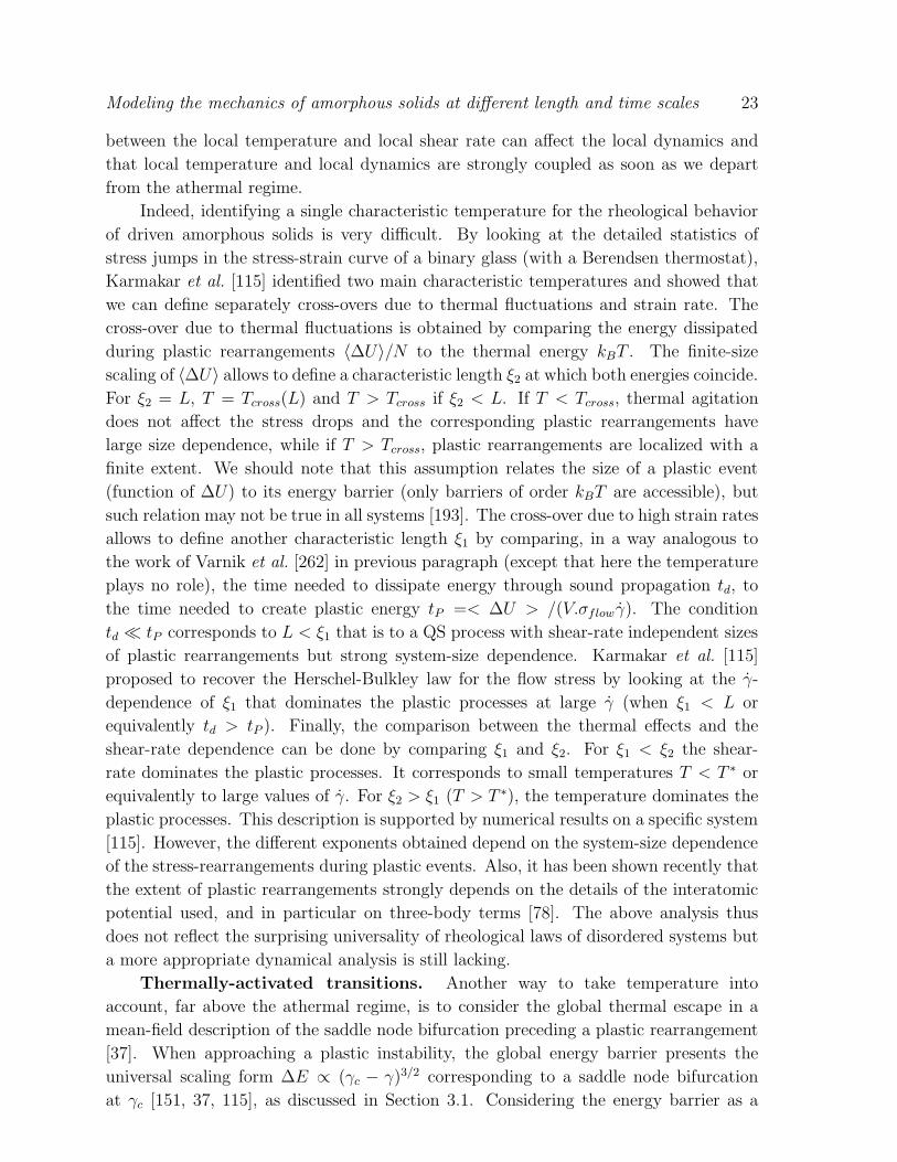
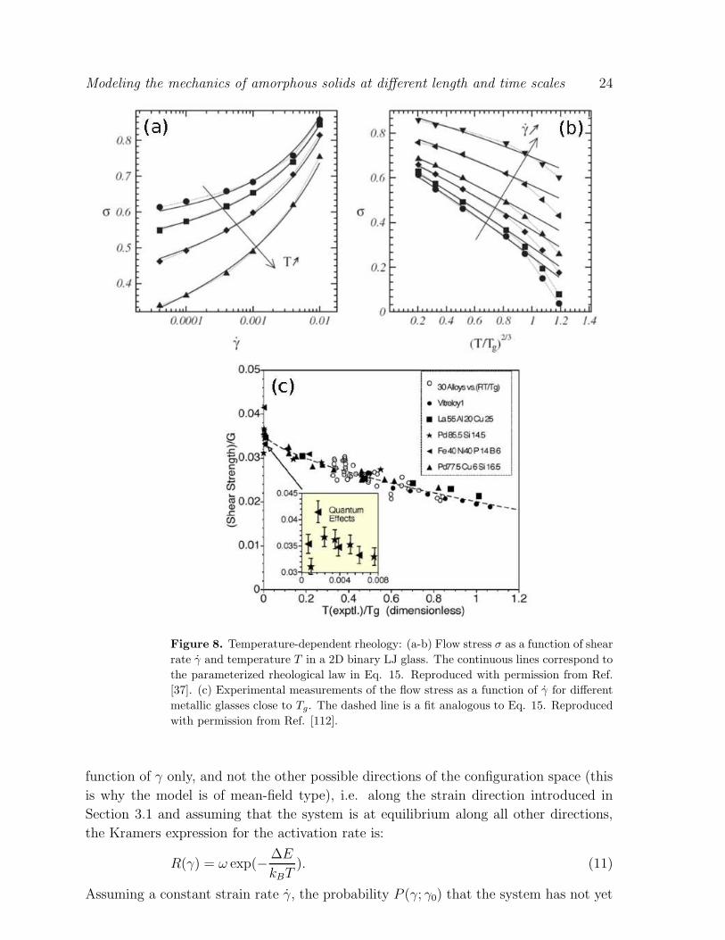
Figure 8. Temperature-dependent rheology: (a-b) Flow stress σ as a function of shear
rate γ and temperature T in a 2D binary LJ glass. The continuous lines correspond to
the parameterized rheological law in Eq. 15. Reproduced with permission from Ref.
[37]. (c) Experimental measurements of the flow stress as a function of γ for different
metallic glasses close to Tg. The dashed line is a fit analogous to Eq. 15. Reproduced
with permission from Ref. [112].
function of γ only, and not the other possible directions of the configuration space (this
is why the model is of mean-field type), i.e. along the strain direction introduced in
Section 3.1 and assuming that the system is at equilibrium along all other directions,
the Kramers expression for the activation rate is:
R(γ) = ω exp(−∆E
kBT). (11)
Assuming a constant strain rate γ, the probability P (γ; γ0) that the system has not yet
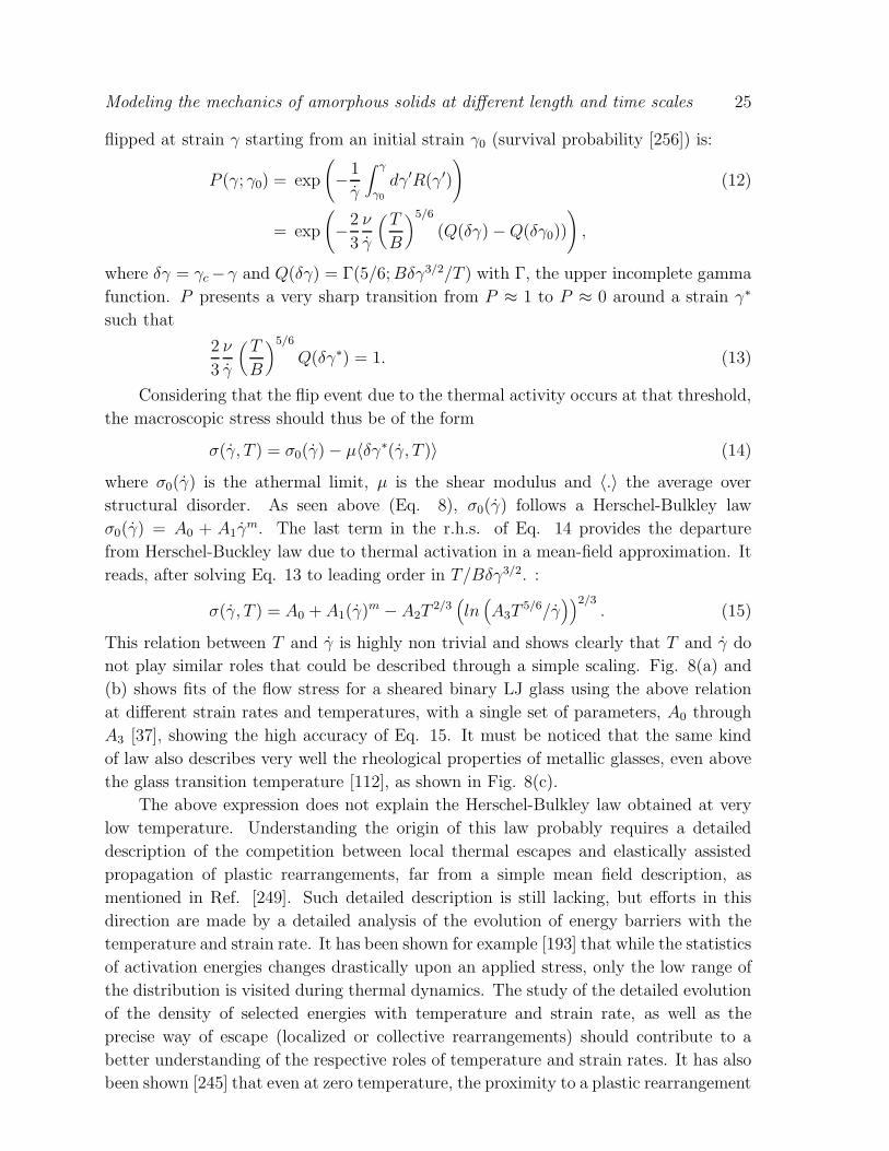
Modeling the mechanics of amorphous solids at different length and time scales 25
flipped at strain γ starting from an initial strain γ0 (survival probability [256]) is:
P (γ; γ0) = exp
(
−1
γ
∫ γ
γ0dγ′R(γ′)
)
(12)
= exp
(
−2
3
ν
γ
(
T
B
)5/6
(Q(δγ)−Q(δγ0))
)
,
where δγ = γc−γ and Q(δγ) = Γ(5/6;Bδγ3/2/T ) with Γ, the upper incomplete gamma
function. P presents a very sharp transition from P ≈ 1 to P ≈ 0 around a strain γ∗
such that
2
3
ν
γ
(
T
B
)5/6
Q(δγ∗) = 1. (13)
Considering that the flip event due to the thermal activity occurs at that threshold,
the macroscopic stress should thus be of the form
σ(γ, T ) = σ0(γ)− µ〈δγ∗(γ, T )〉 (14)
where σ0(γ) is the athermal limit, µ is the shear modulus and 〈.〉 the average over
structural disorder. As seen above (Eq. 8), σ0(γ) follows a Herschel-Bulkley law
σ0(γ) = A0 + A1γm. The last term in the r.h.s. of Eq. 14 provides the departure
from Herschel-Buckley law due to thermal activation in a mean-field approximation. It
reads, after solving Eq. 13 to leading order in T/Bδγ3/2. :
σ(γ, T ) = A0 + A1(γ)m − A2T
2/3(
ln(
A3T5/6/γ
))2/3. (15)
This relation between T and γ is highly non trivial and shows clearly that T and γ do
not play similar roles that could be described through a simple scaling. Fig. 8(a) and
(b) shows fits of the flow stress for a sheared binary LJ glass using the above relation
at different strain rates and temperatures, with a single set of parameters, A0 through
A3 [37], showing the high accuracy of Eq. 15. It must be noticed that the same kind
of law also describes very well the rheological properties of metallic glasses, even above
the glass transition temperature [112], as shown in Fig. 8(c).
The above expression does not explain the Herschel-Bulkley law obtained at very
low temperature. Understanding the origin of this law probably requires a detailed
description of the competition between local thermal escapes and elastically assisted
propagation of plastic rearrangements, far from a simple mean field description, as
mentioned in Ref. [249]. Such detailed description is still lacking, but efforts in this
direction are made by a detailed analysis of the evolution of energy barriers with the
temperature and strain rate. It has been shown for example [193] that while the statistics
of activation energies changes drastically upon an applied stress, only the low range of
the distribution is visited during thermal dynamics. The study of the detailed evolution
of the density of selected energies with temperature and strain rate, as well as the
precise way of escape (localized or collective rearrangements) should contribute to a
better understanding of the respective roles of temperature and strain rates. It has also
been shown [245] that even at zero temperature, the proximity to a plastic rearrangement
Modeling the mechanics of amorphous solids at different length and time scales 26
(quadrupolar rearrangement or elementary shear band) affects not only the low energy
distribution of activation energies, but also the low frequency eigenmodes of the system,
and thus the detailed accessible rearrangements. The respective occurrence of thermal
escapes and mechanical vanishing of activation barriers can thus give rise to a variety
of different behaviors.
Effective temperature. A general way to take into account the different roles of
thermal and mechanical activity is to introduce an effective temperature. This tempting
reconciling view is possible when the average behavior of the system can be described
in terms of the linear response theory, with a linear relation between the response
function to a perturbation and the corresponding correlation function – as in the usual
Fluctuation-Dissipation theorem [46]. In this situation, it has been shown with MD
simulations that the fluctuations in the steady-state flow regime of sheared binary LJ
glasses [23, 22] and model foams [175] are comparable to those in equilibrium systems
maintained at an effective temperature higher than the true temperature and function
of the shear rate. More precisely, when the true temperature is above TC (supercooled
regime), the effective temperature converges to the true temperature T as the strain
rate goes to zero, while for true temperatures below TC (glassy regime), the effective
temperature remains above TC , with a limiting value different from T and close to TC
when the strain rate goes to zero [91]. In addition to steady-state fluctuations, the rate
of activated transitions above energy barriers [103] as well as the steady-state stresses
[91] are also functions of the effective temperature Teff with Arrhenius dependence
of the form exp(−∆E/kBTeff ). However, strong deviations from the linear behavior
may appear, especially when the fluctuations become slow variables [203]. Moreover,
as evidenced by Eq. 15, temperature and strain rate do not play equivalent roles in
thermally-activated transitions. Finally, the average energy of ISs visited in a sheared
system at a given effective temperature is higher than the average IS energy of the same
system maintained in equilibrium at a temperature equal to the effective temperature
[91]. The range of validity of the effective temperature description thus still needs to be
delimited clearly in out-of-equilibrium systems.
Polarization. Another reason why heating and mechanical deformation cannot
be strictly equivalent is that plastic deformation can induce anisotropy in the glass
microstructure whereas heating cannot. Structural anisotropy is referred to as
polarization [12] and is the hallmark of history-dependence in glasses. It is at the
origin of several of the mechanical characteristics of glasses, such as the Baushinger
effect [72] and anelasticity, i.e. time- and temperature-dependent recovery of glasses
after deformation [9, 12]. Polarization has been measured experimentally in metallic
glasses through x-ray diffraction spectra that become anisotropic after plastic flow
in uniaxial tension [236] and compression [176]. The results indicate that during
deformation bonds are reorganized such that in tension, bonds in the tensile direction
are cut and reform in the transverse direction, and vice versa in compression. Bond
anisotropy has been reported in MD simulations of a silica glass [198] by considering
the fabric tensor F = 〈n ⊗ n〉, where n is the unitary bond vector between atoms,
Modeling the mechanics of amorphous solids at different length and time scales 27
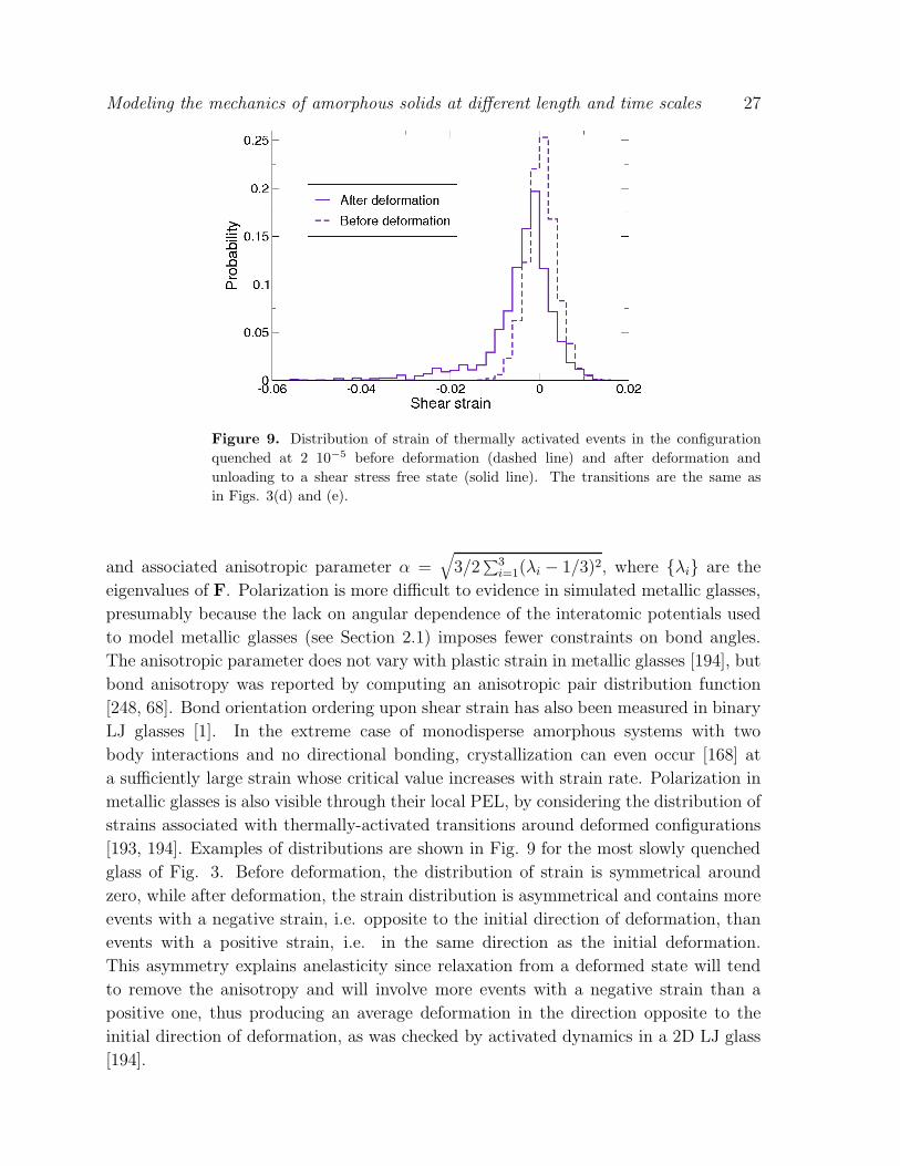
Figure 9. Distribution of strain of thermally activated events in the configuration
quenched at 2 10−5 before deformation (dashed line) and after deformation and
unloading to a shear stress free state (solid line). The transitions are the same as
in Figs. 3(d) and (e).
and associated anisotropic parameter α =√
3/2∑
3
i=1(λi − 1/3)2, where λi are the
eigenvalues of F. Polarization is more difficult to evidence in simulated metallic glasses,
presumably because the lack on angular dependence of the interatomic potentials used
to model metallic glasses (see Section 2.1) imposes fewer constraints on bond angles.
The anisotropic parameter does not vary with plastic strain in metallic glasses [194], but
bond anisotropy was reported by computing an anisotropic pair distribution function
[248, 68]. Bond orientation ordering upon shear strain has also been measured in binary
LJ glasses [1]. In the extreme case of monodisperse amorphous systems with two
body interactions and no directional bonding, crystallization can even occur [168] at
a sufficiently large strain whose critical value increases with strain rate. Polarization in
metallic glasses is also visible through their local PEL, by considering the distribution of
strains associated with thermally-activated transitions around deformed configurations
[193, 194]. Examples of distributions are shown in Fig. 9 for the most slowly quenched
glass of Fig. 3. Before deformation, the distribution of strain is symmetrical around
zero, while after deformation, the strain distribution is asymmetrical and contains more
events with a negative strain, i.e. opposite to the initial direction of deformation, than
events with a positive strain, i.e. in the same direction as the initial deformation.
This asymmetry explains anelasticity since relaxation from a deformed state will tend
to remove the anisotropy and will involve more events with a negative strain than a
positive one, thus producing an average deformation in the direction opposite to the
initial direction of deformation, as was checked by activated dynamics in a 2D LJ glass
[194].
Modeling the mechanics of amorphous solids at different length and time scales 28
4. Mesoscopic models
From the atomistic simulations reviewed above, we know that plasticity in glasses
occurs by local plastic rearrangements, or shear transformations (ST), that have a
characteristic size ℓST on the order of a few nanometers. The cost for the high level
of details in atomistic simulations is a strong limitation in both length- and time
scales (typically a few tens of nanometers during a few tens of nanoseconds as seen
in previous Section). In order to access larger length- and time-scales while retaining
a description of the elementary dissipative plastic processes, we wish now to develop
a model for amorphous plasticity at the mesoscopic scale that averages out atomistic
effects and accounts only for the dynamics of shear transformations, in the same way as
Dislocation Dynamics describes crystal plasticity based on the motion, multiplication
and interaction of dislocations without explicitly accounting for atomic-scale core effects
[146].
Generally speaking, a mesoscopic model requires four elementary ingredients: (i) a
local yield criterion for the occurrence of plastic rearrangements, (ii) an elastic coupling
to represent the reaction of the elastic matrix to the local rearrangements of the
amorphous structure, (iii) an evolution rule for the local yield criterion because a plastic
rearrangement alters locally the amorphous structure, leading to either local softening or
hardening of the matrix, (iv) a dynamical rule to associate a time scale to the elementary
processes. In analogy with atomistic simulations, depending on whether the temperature
range considered is far below or close to the glass transition, the simulations can be
conducted in the athermal quasi-static limit or time and temperature may be accounted
for by using a kinetic Monte Carlo algorithm. The above elementary ingredients are
reviewed below.
As an introductory illustration, directly inspired by the work of Dahmen et
al. [75, 48] and more generally by depinning models of driven interfaces in random
media [141, 114], we present below a general equation of motion that incorporates the
elementary building blocks mentioned above:
η∂ε(x, t)
∂t= Hσext + σint(x, t)− σγ [ε,x, ε(x, t
′ < t)] , (16)
where
σint(x, t) =∫ t
0
dt′∫
dx′J(x− x′, t− t′)[ε(x′, t′)− ε(x, t)] . (17)
We are here restricted to a scalar formulation where ε is the local shear strain, σext
is an applied shear stress, σint is the local shear stress accumulated at point x and time t
due to elastic stress transfer from all previous STs since time t = 0 (where a fully relaxed
– unstressed – configuration is assumed) and σγ is a random pinning stress (local yield
stress) that prevents plastic slip until the local stress (σ = σext + σint) exceeds the local
threshold. η is an effective viscosity that sets the characteristic relaxation rate and H is
the Heaviside step function. This generic example shows how one may build an equation
of motion from a small number of hypothesis in terms of a mesoscopic description of
Modeling the mechanics of amorphous solids at different length and time scales 29
threshold criteria, elastic coupling and dynamics, that can then be solved numerically
– or sometimes analytically.
4.1. Elementary ingredients of a mesoscopic model
Local yield criterion. A mesoscopic model involves a discretization length, ξ, and
the first question to be asked is how to choose ξ with respect to ℓST . This choice
does not appear clearly in the definition of most models proposed in the literature and
ξ may actually be either close to or significantly larger than ℓST , depending on the
model considered. Related to the choice of ξ is the question of using whether a local
or non-local yield criterion for the plastic reorganizations and on what internal variable
should the criterion be based. Indeed, at the continuous scale, all plastic criteria so
far have relied on the local stress state of the material. The well-known Tresca and
von Mises criteria for instance impose a limit, or yield surface, to well-chosen norms
of the deviatoric part of the local stress tensor (maximum deviatoric stress for Tresca,
and maximum deviatoric elastic energy for von Mises). More elaborated criteria can be
defined to take into account the pressure dependence [219, 195, 119]. On the other hand,
at the atomistic scale, we have seen in Section 3.1 that a stress-based criterion for ST
nucleation is not the most relevant because plastic reorganizations are better predicted
by a lowering of the local elastic shear modulus, which is a non-local quantity.
Relating non-local effects and elastic moduli-based criteria at the atomic scale to the
well-established relevance of local stresses at the continuous scale is a very challenging
task that has so far received little attention in the literature, probably due to its inherent
difficulty. One way to circumvent (or reformulate) this question is to identify the relevant
spatial scale ξ at which mesoscopic modeling may be performed. Indeed, one may expect
that non-local contributions that are significant at the reorganization length scale ℓSTare averaged out in a description at a slightly larger length scale (say 10ℓST ≈ 3 nm in
a mineral glass), while preserving the information on the dissipative reorganization due
to the shear transformations.
In practice, mesoscopic models assume homogeneous linear elasticity, such that the
discrete scale ξ should be significantly larger than the microscopic length scale ℓST .
Then, mostly for the sake of simplicity, most models assume a simple (scalar) stress-
based criterion:
σ(x) = σY (x) (18)
where σ is the local shear stress (or shear stress invariant of the stress tensor) and σY is
the local yield stress at location x, also called slip or failure stress, i.e. a ST is triggered
at x if σ(x) > σY (x). The local yield stress can be chosen spatially homogeneous
[186, 187] or heterogeneous [18, 238, 107, 48], with consequences discussed below.
An alternative way that includes thermal activation, is based on an energy approach
at the ST scale [30, 31, 32, 99, 98]. While keeping the hypothesis of elastic homogeneity,
the authors used a lattice defined at a sub-ST scale (ξ < ℓST ) and estimated the energetic
Modeling the mechanics of amorphous solids at different length and time scales 30
cost of local plastic shears involving sets of neighboring cells to recover a length scale
∼ ℓST . The energy cost is computed as:
∆E = ∆F0 − σ(x)γpΩ0
2, (19)
where ∆F0 is the stress-free activation free energy of a ST, biased by the work of the
local stress between the initial and activated configurations, −σΩ∗, where σ is the local
stress resolved on the plane and direction of shear of the ST and Ω∗ = γpΩ0/2 the
activation volume with γp the strain associated with the ST and Ω0 the volume of the
ST. In Ref. [99], the plastic strain increment γp was chosen constant, equal to 0.1 in
agreement with the Lindemann criterion observed at the atomic scale (see Section 3.1).
The volume of the ST Ω0 was also constant, taken equal to 1.6 nm3 to reproduce the
properties of Vitreloy 1, a commercial metallic glass, i.e. contains 84 atoms, again in
agreement with the atomistic simulations presented in Section 3.1. We should note
that within this approach, if an athermal yield criterion is applied, stating that plastic
events occur when their activation energy vanishes, a local homogeneous stress-based
yield criterion is recovered, as in Eq. 18, with a yield stress σY = ∆F0/Ω∗.
Evolution rule for the yield criterion. Another crucial point concerns
the evolution of the criterion landscape under plastic deformation. Indeed, after a
reorganization has occurred, the local structure of the glass is altered, which may change
its local yield stress. In some models proposed in the literature, the local yield stress
in Eq. 18 is unchanged after plastic slip [30, 186, 187, 99, 98] implying a homogeneous
and stationary yield stress landscape. In other models, the yield stress is renewed
based on a specific rule: the new value may be drawn from a stationary distribution
without correlation [18, 238] or may be systematically increased (resp. decreased) [48],
which naturally leads to hardening (resp. softening). We should note that using a
stationary distribution also leads to hardening during the initial stage of deformation by
a progressive exhaustion of the weakest sites in the configuration [238]. Two different
distributions (one for the initial configuration and the other for renewing the yield
stresses under deformation) have also been used to model aging [258] (see below).
Elastic coupling. Successive shear transformations are not independent because
the elastic medium surrounding the reorganizing zone reacts to the local change of
conformation and acquires an additional (positive or negative) internal stress increment.
The strength of this increment depends on the plastic strain associated with the ST, the
size of the ST and the shear modulus [237]. While ST size and shear modulus have been
so far systematically chosen constant, the plastic strain has been chosen either constant
[30, 99] or drawn from a statistical distribution [18, 238].
Restricting ourselves to continuum mechanics, finding the elastic relaxation around
a plastic shear transformation is similar to the plastic inclusion problem treated early-on
by Eshelby [70]. We will assume here as in previous paragraphs that the mesoscopic
length scale is sufficiently large to allow for a continuum and homogeneous description
of elasticity. Within this approximation, there are several ways to include elastic effects
in mesoscopic models:
Modeling the mechanics of amorphous solids at different length and time scales 31
• Mean Field. Ignoring the details of the elastic interaction, a first approach consists
in assuming that the elastic relaxation of a reorganized region is compensated by a
constant elastic stress everywhere else [48]. A statistical variant consists in drawing
local elastic responses from an uncorrelated random distribution (constrained by
the global balance of elastic contributions). Several distributions have been tested
[134], from a simple Gaussian distribution to ad-hoc distributions that mimic the
effect of a quadrupolar Eshelby contribution (see below). An advantage of this
approach is the possibility for analytical treatment [260, 134].
• Exact numerical solution. A second approach consists in solving numerically the
equation of elastic equilibrium, thus accounting for the precise plastic strain induced
by the ST and the outer boundary conditions. Elasticity can be solved using the
finite element method in direct space [99] or, if the lattice is regular, using Green’s
function, obtained as the elastic response of an elementary cell of the lattice to a
unit shear [30, 18], or else using Lagrange multipliers [107].
• Eshelby quadrupolar interaction. An intermediate way consists in focusing on the
dominant term of the elastic response at long distance. The Eshelby solution of
the elastic field induced by a plastic inclusion can be developed using a multipolar
expansion [237]. While at short distance several terms are necessary to account for
the details of the plastic reorganizations, at long distance, only the dominant term
of the expansion, proportional to 1/rd (where d is the space dimension) survives.
In two dimensions, such an analysis can be carried out using the complex potentials
of Kolossov and Muskhelishvili [171]. It appears that only two terms survive
at long distance. One is associated with the temporary dilation/contraction of
a circular inclusion while the other term is associated with the local shear of a
circular inclusion. This second term is responsible for the well-known quadrupolar
symmetry of the elastic shear stress response:
σxy = −2µ
κ+ 1
Aγpπr2
cos(4θ) (20)
where µ is the elastic shear modulus and κ = (3 − 4ν) for plane strain and
κ = (3− ν)/(1 + ν) for plane stress, ν being the Poisson’s ratio. This symmetry is
visible for example in the atomistic snapshot shown in Fig. 1(a). Note that in Eq.
20, the size of the zone under reorganization A does not contribute independently
but through its product with the plastic strain, which is about twice the activation
surface or activation volume in Eq. 19. γp being on the order of 0.1, the activation
volume or surface is about a tenth of its actual size, in contrast with dislocations
where γp is close to 1 and activation and real surfaces and volumes are identical.
While a priori simple, the implementation of such quadrupolar solution on a
discrete lattice happens to be numerically delicate. Satisfaction of the boundary
conditions is made difficult by the long-range decay of the elastic interaction. To
circumvent potential resummation problems in direct space, it is valuable to rewrite
the interaction in Fourier space in case of periodic boundary conditions [187, 238].
Modeling the mechanics of amorphous solids at different length and time scales 32
Dynamical rule. As mentioned above, there are two main choices of dynamical
rule for mesoscopic models, based on either a quasi-static or a kinetic Monte Carlo
algorithm. In the quasi-static limit, thermal and rate effects are ignored and the
dynamics is entirely dictated by the satisfaction of the local yield criterion. The system
can be either stress- or strain-driven using two simple numerical protocols inherited
from the field of self-consistent criticality [222, 178]. The first protocol, called extremal
dynamics [18, 238], consists in allowing one and only one event per simulation step, i.e.
the weakest site in the configuration. The applied stress (called extremal stress) is thus
adapted at each step to induce only this event and therefore accommodates a vanishing
shear rate. In the algorithm, the weakest site is first identified and subjected to a
local plastic strain, the associated local yield stress is renewed (or not) according to the
chosen rule of evolution and the stress field is updated to account for the internal stress
change induced by the local transformation. Finally the whole process is iterated. While
the shear strain rate is reduced at its lowest possible numerical value, the associated
extremal stress strongly fluctuates. The macroscopic yield stress is then identified as
the maximum extremal stress.
The second quasi-static protocol consists in slowly (quasi-statically) increasing the
applied stress [187, 48]. For a given value of the external stress, all sites satisfying their
local yield criterion experience a shear strain increment. As before, the yield criterion
and internal stress are then updated, but in contrast with before, the applied stress is
unchanged. Thus, the new configuration may contain a new set of sites that satisfy the
yield criterion, i.e. the occurrence of some local slip may trigger other local slip events,
leading to avalanches, as seen in the atomistic simulations in Section 3.1. The procedure
is then iterated at constant applied stress until the avalanche eventually stops, when
a configuration is reached where no site satisfies the yield criterion. Only then is the
external stress increased by a small amount and the whole procedure is started again.
In this approach, the number of sites experiencing slip increases with external stress
and diverges when the macroscopic yield stress is reached [187]. Note that the bulk
elasticity of the material and/or the compliance of the mechanical testing machine can
be incorporated by coupling the system to a spring [243, 273]. Tuning the value of the
spring constant then allows to drive the system either close to extremal dynamics (high
spring constant) or to a slowly increasing stress (low spring constant).
The above protocols suffer from a clear drawback: any notion of realistic time
has disappeared since the number of iterations simply counts the number of plastic
rearrangements and avalanches in the system; or said in other words, while the iterations
give successive configurations of the system, the time scale separating the configurations
is unknown. One way to introduce a time scale and at the same time thermal
effects is to employ a kinetic Monte Carlo algorithm. This approach has been used
in conjunction with the energy-based criterion in Eq. 19, which provides the activation
energy of potentially thermally-activated STs [30, 99, 98]. From a given configuration,
all potentially thermally-activated events are first determined. The activation energy of
each event is calculated, from which the distribution of rates of the events is obtained
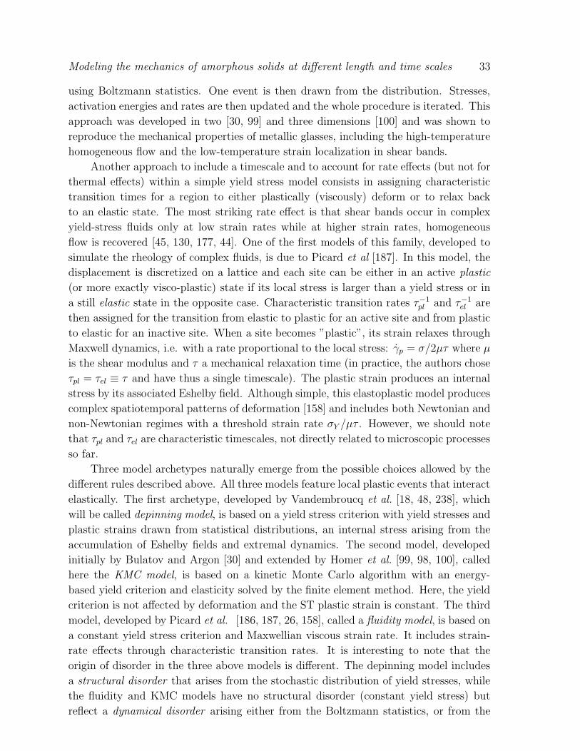
Modeling the mechanics of amorphous solids at different length and time scales 33
using Boltzmann statistics. One event is then drawn from the distribution. Stresses,
activation energies and rates are then updated and the whole procedure is iterated. This
approach was developed in two [30, 99] and three dimensions [100] and was shown to
reproduce the mechanical properties of metallic glasses, including the high-temperature
homogeneous flow and the low-temperature strain localization in shear bands.
Another approach to include a timescale and to account for rate effects (but not for
thermal effects) within a simple yield stress model consists in assigning characteristic
transition times for a region to either plastically (viscously) deform or to relax back
to an elastic state. The most striking rate effect is that shear bands occur in complex
yield-stress fluids only at low strain rates while at higher strain rates, homogeneous
flow is recovered [45, 130, 177, 44]. One of the first models of this family, developed to
simulate the rheology of complex fluids, is due to Picard et al [187]. In this model, the
displacement is discretized on a lattice and each site can be either in an active plastic
(or more exactly visco-plastic) state if its local stress is larger than a yield stress or in
a still elastic state in the opposite case. Characteristic transition rates τ−1
pl and τ−1
el are
then assigned for the transition from elastic to plastic for an active site and from plastic
to elastic for an inactive site. When a site becomes ”plastic”, its strain relaxes through
Maxwell dynamics, i.e. with a rate proportional to the local stress: γp = σ/2µτ where µ
is the shear modulus and τ a mechanical relaxation time (in practice, the authors chose
τpl = τel ≡ τ and have thus a single timescale). The plastic strain produces an internal
stress by its associated Eshelby field. Although simple, this elastoplastic model produces
complex spatiotemporal patterns of deformation [158] and includes both Newtonian and
non-Newtonian regimes with a threshold strain rate σY /µτ . However, we should note
that τpl and τel are characteristic timescales, not directly related to microscopic processes
so far.
Three model archetypes naturally emerge from the possible choices allowed by the
different rules described above. All three models feature local plastic events that interact
elastically. The first archetype, developed by Vandembroucq et al. [18, 48, 238], which
will be called depinning model, is based on a yield stress criterion with yield stresses and
plastic strains drawn from statistical distributions, an internal stress arising from the
accumulation of Eshelby fields and extremal dynamics. The second model, developed
initially by Bulatov and Argon [30] and extended by Homer et al. [99, 98, 100], called
here the KMC model, is based on a kinetic Monte Carlo algorithm with an energy-
based yield criterion and elasticity solved by the finite element method. Here, the yield
criterion is not affected by deformation and the ST plastic strain is constant. The third
model, developed by Picard et al. [186, 187, 26, 158], called a fluidity model, is based on
a constant yield stress criterion and Maxwellian viscous strain rate. It includes strain-
rate effects through characteristic transition rates. It is interesting to note that the
origin of disorder in the three above models is different. The depinning model includes
a structural disorder that arises from the stochastic distribution of yield stresses, while
the fluidity and KMC models have no structural disorder (constant yield stress) but
reflect a dynamical disorder arising either from the Boltzmann statistics, or from the
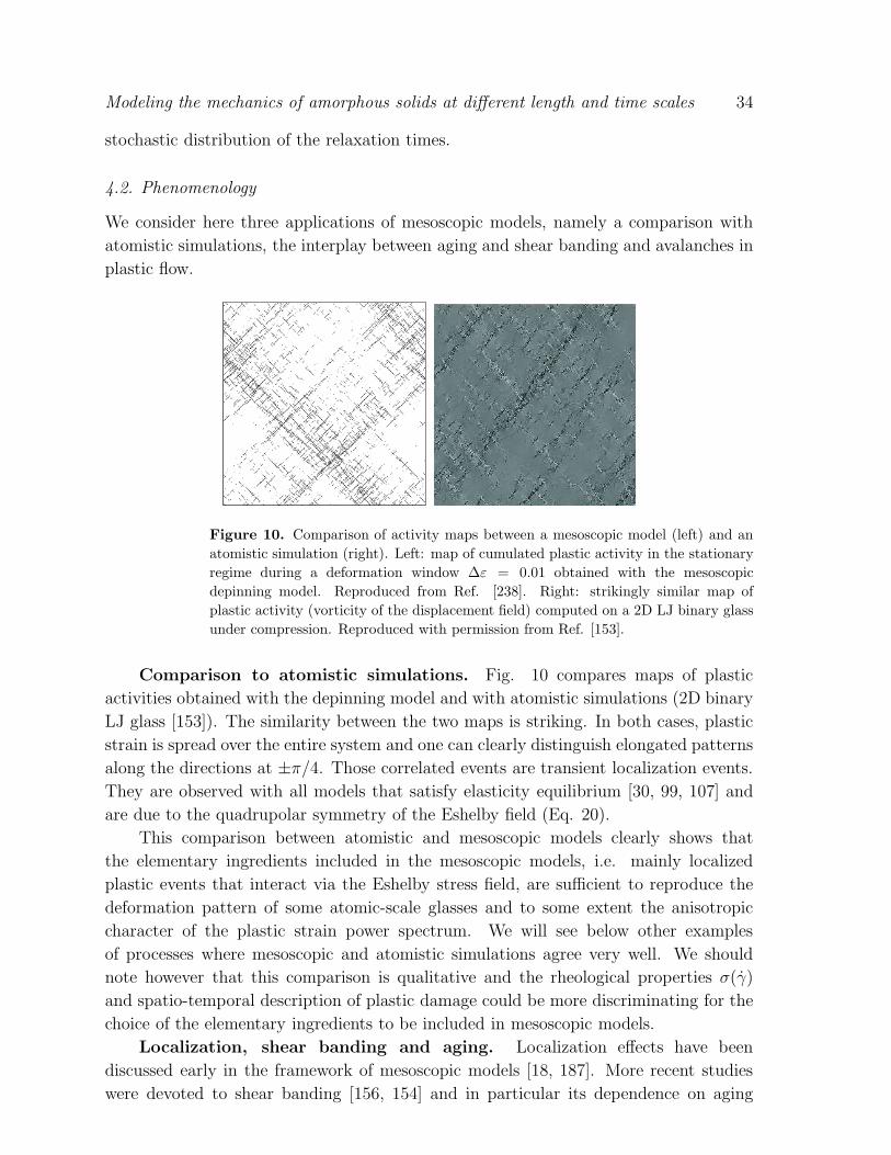
Modeling the mechanics of amorphous solids at different length and time scales 34
stochastic distribution of the relaxation times.
4.2. Phenomenology
We consider here three applications of mesoscopic models, namely a comparison with
atomistic simulations, the interplay between aging and shear banding and avalanches in
plastic flow.
Figure 10. Comparison of activity maps between a mesoscopic model (left) and an
atomistic simulation (right). Left: map of cumulated plastic activity in the stationary
regime during a deformation window ∆ε = 0.01 obtained with the mesoscopic
depinning model. Reproduced from Ref. [238]. Right: strikingly similar map of
plastic activity (vorticity of the displacement field) computed on a 2D LJ binary glass
under compression. Reproduced with permission from Ref. [153].
Comparison to atomistic simulations. Fig. 10 compares maps of plastic
activities obtained with the depinning model and with atomistic simulations (2D binary
LJ glass [153]). The similarity between the two maps is striking. In both cases, plastic
strain is spread over the entire system and one can clearly distinguish elongated patterns
along the directions at ±π/4. Those correlated events are transient localization events.
They are observed with all models that satisfy elasticity equilibrium [30, 99, 107] and
are due to the quadrupolar symmetry of the Eshelby field (Eq. 20).
This comparison between atomistic and mesoscopic models clearly shows that
the elementary ingredients included in the mesoscopic models, i.e. mainly localized
plastic events that interact via the Eshelby stress field, are sufficient to reproduce the
deformation pattern of some atomic-scale glasses and to some extent the anisotropic
character of the plastic strain power spectrum. We will see below other examples
of processes where mesoscopic and atomistic simulations agree very well. We should
note however that this comparison is qualitative and the rheological properties σ(γ)
and spatio-temporal description of plastic damage could be more discriminating for the
choice of the elementary ingredients to be included in mesoscopic models.
Localization, shear banding and aging. Localization effects have been
discussed early in the framework of mesoscopic models [18, 187]. More recent studies
were devoted to shear banding [156, 154] and in particular its dependence on aging
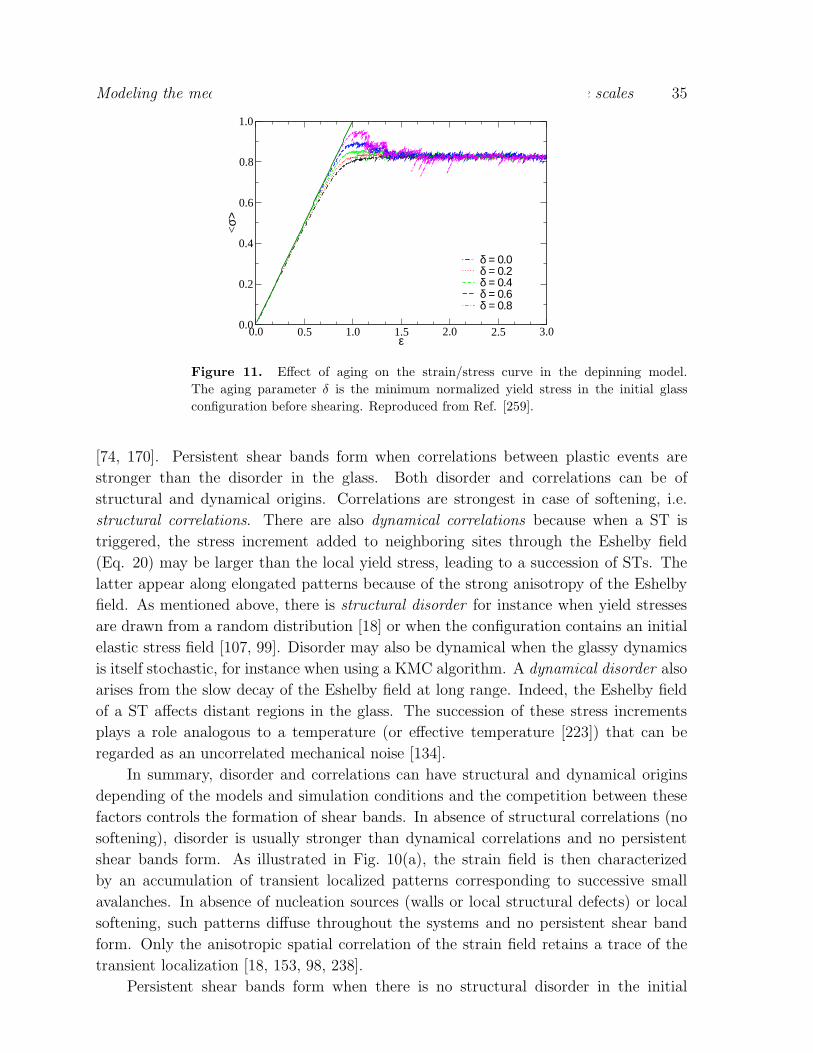
Modeling the mechanics of amorphous solids at different length and time scales 35
0.0 0.5 1.0 1.5 2.0 2.5 3.0ε
0.0
0.2
0.4
0.6
0.8
1.0
<σ>
δ = 0.0δ = 0.2δ = 0.4δ = 0.6δ = 0.8
Figure 11. Effect of aging on the strain/stress curve in the depinning model.
The aging parameter δ is the minimum normalized yield stress in the initial glass
configuration before shearing. Reproduced from Ref. [259].
[74, 170]. Persistent shear bands form when correlations between plastic events are
stronger than the disorder in the glass. Both disorder and correlations can be of
structural and dynamical origins. Correlations are strongest in case of softening, i.e.
structural correlations. There are also dynamical correlations because when a ST is
triggered, the stress increment added to neighboring sites through the Eshelby field
(Eq. 20) may be larger than the local yield stress, leading to a succession of STs. The
latter appear along elongated patterns because of the strong anisotropy of the Eshelby
field. As mentioned above, there is structural disorder for instance when yield stresses
are drawn from a random distribution [18] or when the configuration contains an initial
elastic stress field [107, 99]. Disorder may also be dynamical when the glassy dynamics
is itself stochastic, for instance when using a KMC algorithm. A dynamical disorder also
arises from the slow decay of the Eshelby field at long range. Indeed, the Eshelby field
of a ST affects distant regions in the glass. The succession of these stress increments
plays a role analogous to a temperature (or effective temperature [223]) that can be
regarded as an uncorrelated mechanical noise [134].
In summary, disorder and correlations can have structural and dynamical origins
depending of the models and simulation conditions and the competition between these
factors controls the formation of shear bands. In absence of structural correlations (no
softening), disorder is usually stronger than dynamical correlations and no persistent
shear bands form. As illustrated in Fig. 10(a), the strain field is then characterized
by an accumulation of transient localized patterns corresponding to successive small
avalanches. In absence of nucleation sources (walls or local structural defects) or local
softening, such patterns diffuse throughout the systems and no persistent shear band
form. Only the anisotropic spatial correlation of the strain field retains a trace of the
transient localization [18, 153, 98, 238].
Persistent shear bands form when there is no structural disorder in the initial
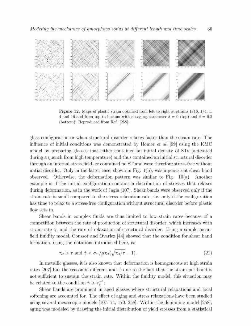
Modeling the mechanics of amorphous solids at different length and time scales 36
Figure 12. Maps of plastic strain obtained from left to right at strains 1/16, 1/4, 1,
4 and 16 and from top to bottom with an aging parameter δ = 0 (top) and δ = 0.5
(bottom). Reproduced from Ref. [258].
glass configuration or when structural disorder relaxes faster than the strain rate. The
influence of initial conditions was demonstrated by Homer et al. [99] using the KMC
model by preparing glasses that either contained an initial density of STs (activated
during a quench from high temperature) and thus contained an initial structural disorder
through an internal stress field, or contained no ST and were therefore stress-free without
initial disorder. Only in the latter case, shown in Fig. 1(b), was a persistent shear band
observed. Otherwise, the deformation pattern was similar to Fig. 10(a). Another
example is if the initial configuration contains a distribution of stresses that relaxes
during deformation, as in the work of Jagla [107]. Shear bands were observed only if the
strain rate is small compared to the stress-relaxation rate, i.e. only if the configuration
has time to relax to a stress-free configuration without structural disorder before plastic
flow sets in.
Shear bands in complex fluids are thus limited to low strain rates because of a
competition between the rate of production of structural disorder, which increases with
strain rate γ, and the rate of relaxation of structural disorder. Using a simple mean-
field fluidity model, Coussot and Ovarlez [44] showed that the condition for shear band
formation, using the notations introduced here, is:
τel > τ and γ < σY /µτel(√
τel/τ − 1). (21)
In metallic glasses, it is also known that deformation is homogeneous at high strain
rates [207] but the reason is different and is due to the fact that the strain per band is
not sufficient to sustain the strain rate. Within the fluidity model, this situation may
be related to the condition γ > τ−1
pl .
Shear bands are prominent in aged glasses where structural relaxations and local
softening are accounted for. The effect of aging and stress relaxations have been studied
using several mesoscopic models [107, 74, 170, 258]. Within the depinning model [258],
aging was modeled by drawing the initial distribution of yield stresses from a statistical
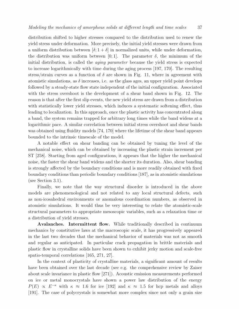
Modeling the mechanics of amorphous solids at different length and time scales 37
distribution shifted to higher stresses compared to the distribution used to renew the
yield stress under deformation. More precisely, the initial yield stresses were drawn from
a uniform distribution between [δ; 1 + δ] in normalized units, while under deformation,
the distribution was uniform between [0; 1]. The parameter δ, the minimum of the
initial distribution, is called the aging parameter because the yield stress is expected
to increase logarithmically with time during the aging process [197, 170]. The resulting
stress/strain curves as a function of δ are shown in Fig. 11, where in agreement with
atomistic simulations, as δ increases, i.e. as the glass ages, an upper yield point develops
followed by a steady-state flow state independent of the initial configuration. Associated
with the stress overshoot is the development of a shear band shown in Fig. 12. The
reason is that after the first slip events, the new yield stress are drawn from a distribution
with statistically lower yield stresses, which induces a systematic softening effect, thus
leading to localization. In this approach, once the plastic activity has concentrated along
a band, the system remains trapped for arbitrary long times while the band widens at a
logarithmic pace. A similar correlation between initial stress overshoot and shear bands
was obtained using fluidity models [74, 170] where the lifetime of the shear band appears
bounded to the intrinsic timescale of the model.
A notable effect on shear banding can be obtained by tuning the level of the
mechanical noise, which can be obtained by increasing the plastic strain increment per
ST [258]. Starting from aged configurations, it appears that the higher the mechanical
noise, the faster the shear band widens and the shorter its duration. Also, shear banding
is strongly affected by the boundary conditions and is more readily obtained with fixed
boundary conditions than periodic boundary conditions [187], as in atomistic simulations
(see Section 3.1).
Finally, we note that the way structural disorder is introduced in the above
models are phenomenological and not related to any local structural defects, such
as non-icosahedral environments or anomalous coordination numbers, as observed in
atomistic simulations. It would thus be very interesting to relate the atomistic-scale
structural parameters to appropriate mesoscopic variables, such as a relaxation time or
a distribution of yield stresses.
Avalanches. Intermittent flow. While traditionally described in continuum
mechanics by constitutive laws at the macroscopic scale, it has progressively appeared
in the last two decades that the mechanical behavior of materials was not as smooth
and regular as anticipated. In particular crack propagation in brittle materials and
plastic flow in crystalline solids have been shown to exhibit jerky motion and scale-free
spatio-temporal correlations [165, 271, 27].
In the context of plasticity of crystalline materials, a significant amount of results
have been obtained over the last decade (see e.g. the comprehensive review by Zaiser
about scale invariance in plastic flow [271]). Acoustic emission measurements performed
on ice or metal monocrystals have shown a power law distribution of the energy
P (E) ∝ E−κ with κ ≈ 1.6 for ice [192] and κ ≈ 1.5 for hcp metals and alloys
[191]. The case of polycrystals is somewhat more complex since not only a grain size
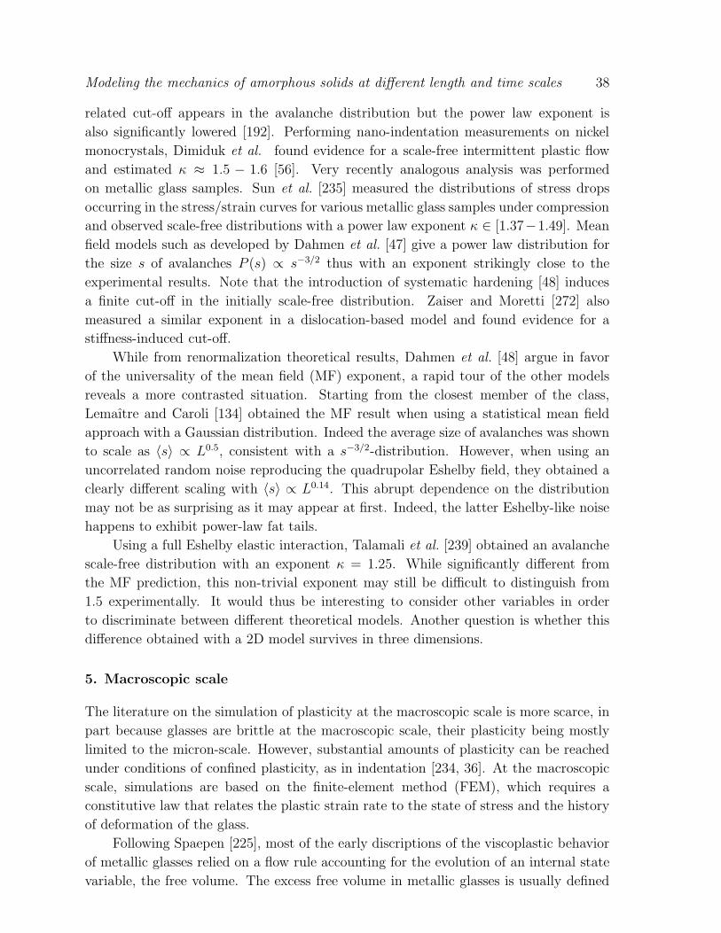
Modeling the mechanics of amorphous solids at different length and time scales 38
related cut-off appears in the avalanche distribution but the power law exponent is
also significantly lowered [192]. Performing nano-indentation measurements on nickel
monocrystals, Dimiduk et al. found evidence for a scale-free intermittent plastic flow
and estimated κ ≈ 1.5 − 1.6 [56]. Very recently analogous analysis was performed
on metallic glass samples. Sun et al. [235] measured the distributions of stress drops
occurring in the stress/strain curves for various metallic glass samples under compression
and observed scale-free distributions with a power law exponent κ ∈ [1.37−1.49]. Mean
field models such as developed by Dahmen et al. [47] give a power law distribution for
the size s of avalanches P (s) ∝ s−3/2 thus with an exponent strikingly close to the
experimental results. Note that the introduction of systematic hardening [48] induces
a finite cut-off in the initially scale-free distribution. Zaiser and Moretti [272] also
measured a similar exponent in a dislocation-based model and found evidence for a
stiffness-induced cut-off.
While from renormalization theoretical results, Dahmen et al. [48] argue in favor
of the universality of the mean field (MF) exponent, a rapid tour of the other models
reveals a more contrasted situation. Starting from the closest member of the class,
Lemaıtre and Caroli [134] obtained the MF result when using a statistical mean field
approach with a Gaussian distribution. Indeed the average size of avalanches was shown
to scale as 〈s〉 ∝ L0.5, consistent with a s−3/2-distribution. However, when using an
uncorrelated random noise reproducing the quadrupolar Eshelby field, they obtained a
clearly different scaling with 〈s〉 ∝ L0.14. This abrupt dependence on the distribution
may not be as surprising as it may appear at first. Indeed, the latter Eshelby-like noise
happens to exhibit power-law fat tails.
Using a full Eshelby elastic interaction, Talamali et al. [239] obtained an avalanche
scale-free distribution with an exponent κ = 1.25. While significantly different from
the MF prediction, this non-trivial exponent may still be difficult to distinguish from
1.5 experimentally. It would thus be interesting to consider other variables in order
to discriminate between different theoretical models. Another question is whether this
difference obtained with a 2D model survives in three dimensions.
5. Macroscopic scale
The literature on the simulation of plasticity at the macroscopic scale is more scarce, in
part because glasses are brittle at the macroscopic scale, their plasticity being mostly
limited to the micron-scale. However, substantial amounts of plasticity can be reached
under conditions of confined plasticity, as in indentation [234, 36]. At the macroscopic
scale, simulations are based on the finite-element method (FEM), which requires a
constitutive law that relates the plastic strain rate to the state of stress and the history
of deformation of the glass.
Following Spaepen [225], most of the early discriptions of the viscoplastic behavior
of metallic glasses relied on a flow rule accounting for the evolution of an internal state
variable, the free volume. The excess free volume in metallic glasses is usually defined
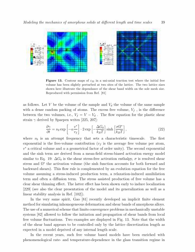
Modeling the mechanics of amorphous solids at different length and time scales 39
Figure 13. Contour maps of ε22 in a uni-axial traction test where the initial free
volume has been slightly perturbed at two sites of the lattice. The two lattice sizes
shown here illustrate the dependance of the shear band width on the sole mesh size.
Reproduced with permission from Ref. [81]
as follows. Let V be the volume of the sample and Vd the volume of the same sample
with a dense random packing of atoms. The excess free volume, Vf , is the difference
between the two volumes, i.e., Vf = V − Vd . The flow equation for the plastic shear
strain γ derived by Spaepen writes [225, 207]:
∂γ
∂t= ν0 exp
[
−αv∗
vf
]
· 2 exp[
−∆G0
kBT
]
sinh[
σΩ∗
kBT
]
, (22)
where ν0 is an attempt frequency that sets a characteristic timescale. The first
exponential is the free-volume contribution (vf is the average free volume per atom,
v∗ a critical volume and α a geometrical factor of order unity). The second exponential
and the sinh term are derived from a mean-field stress-biased activation energy model
similar to Eq. 19: ∆G0 is the shear stress-free activation enthalpy, σ is resolved shear
stress and Ω∗ the activation volume (the sinh function accounts for both forward and
backward shears). This flow rule is complemented by an evolution equation for the free
volume assuming a stress-induced production term, a relaxation-induced annihilation
term and often a diffusion term. The stress assisted production of free volume has a
clear shear thinning effect. The latter effect has been shown early to induce localization
[229] (see also the clear presentation of the model and its generalization as well as a
linear stability analysis in Ref. [102]).
In the very same spirit, Gao [81] recently developed an implicit finite element
method for simulating inhomogeneous deformation and shear bands of amorphous alloys.
The use of a numerical scheme that limits convergence problems in mechanically unstable
systems [82] allowed to follow the initiation and propagation of shear bands from local
free volume fluctuations. Two examples are displayed in Fig. 13. Note that the width
of the shear band appears to be controlled only by the lattice discretization length as
expected in a model deprived of any internal length scale.
In the recent years, such free volume based models have been enriched with
phenomenological rate- and temperature-dependence in the glass transition regime in
Modeling the mechanics of amorphous solids at different length and time scales 40
order to account for the technological thermoplastic forming process[3].
While free volume has been widely used as a shear thinning ingredient, the natural
consequence of stress-induced free volume expansion, i.e.the introduction of an inelastic
volumetric deformation, has been less frequently discussed [76, 102]. A simple reason
for leaving aside this a priori important aspect (after all, while dislocations are volume
conserving, no such limit applies to shear transformations) is that in most experimental
tests performed on metallic glasses, pressure levels remain low compared to the yield
stress value [144]. Strongly contrasting with such a statement is the case of indentation
tests where pressure levels are frequently measured in GigaPascal units.
So far, two main constitutive laws have been proposed to model plasticity during
indentation experiments, one in amorphous silica by Kermouche et al. [119, 183] and the
other in metallic glasses by Anand and Su for low temperatures in the shear banding
regime [4, 234] and for high temperatures in the homogeneous deformation regime
[5]. The main characteristic of these constitutive laws is to account for the pressure-
dependence of the plastic deformation of glasses. However, they treat this effect in
different ways due to the specificities of the glasses considered. For metallic glasses, the
pressure dependence is treated using a Mohr-Coulomb law [144, 131], where the yield
stress in shear increases linearly with the normal stress, while for silica glasses, following
early attempts based on a simple linearly pressure-dependent Mises criterion [128], a
quadratic law involving deviatoric stress and pressure, inspired from the mechanics of
porous materials was employed. In both cases, the pressure dependence is related to
the free-volume in the material but in the case of metallic glasses, plasticity leads to
an increase of free volume and a corresponding softening of the glass, whereas in silica
glasses, plasticity decreases the free volume and induces densification [270, 109] and
hardening [184, 257] of the glass. Finally, in silica glasses, only density hardening was
considered (by a linear relation between the plastic limit in hydrostatic compression
and the plastic strain) while no hardening in shear was accounted for, while in metallic
glasses, shear softening by the increase of free volume was considered, while the Mohr-
Coulomb friction coefficient was held constant, implying no density hardening (or
softening). The hypothesis used in both constitutive laws are thus quite different but
well-adapted to the systems considered since in both cases, the simulations were at
least in qualitative agreement with experiments. In particular, in silica glasses, the
authors were able to reproduce densification maps below the indentor, while in metallic
glasses, the simulations showed shear band patterns, as shown in Fig. 1(c), in good
agreement with experiments and atomic-scale simulations [214, 216] In the perspective
of multiscale modeling, the constitutive laws could also be checked directly by MD
simulations on submicrometric samples submitted to different kinds of deformations,
like shear at constant pressure or hydrostatic compression.
Finally, remaining in the framework of mutiscale modeling, an additional interesting
point of comparison is given by recent works simulating the plastic behavior of bulk
amorphous matrix composites [131]. In the very same spirit as glass-ceramics developed
to improve mechanical properties of oxide glasses, such materials incorporate nano- or
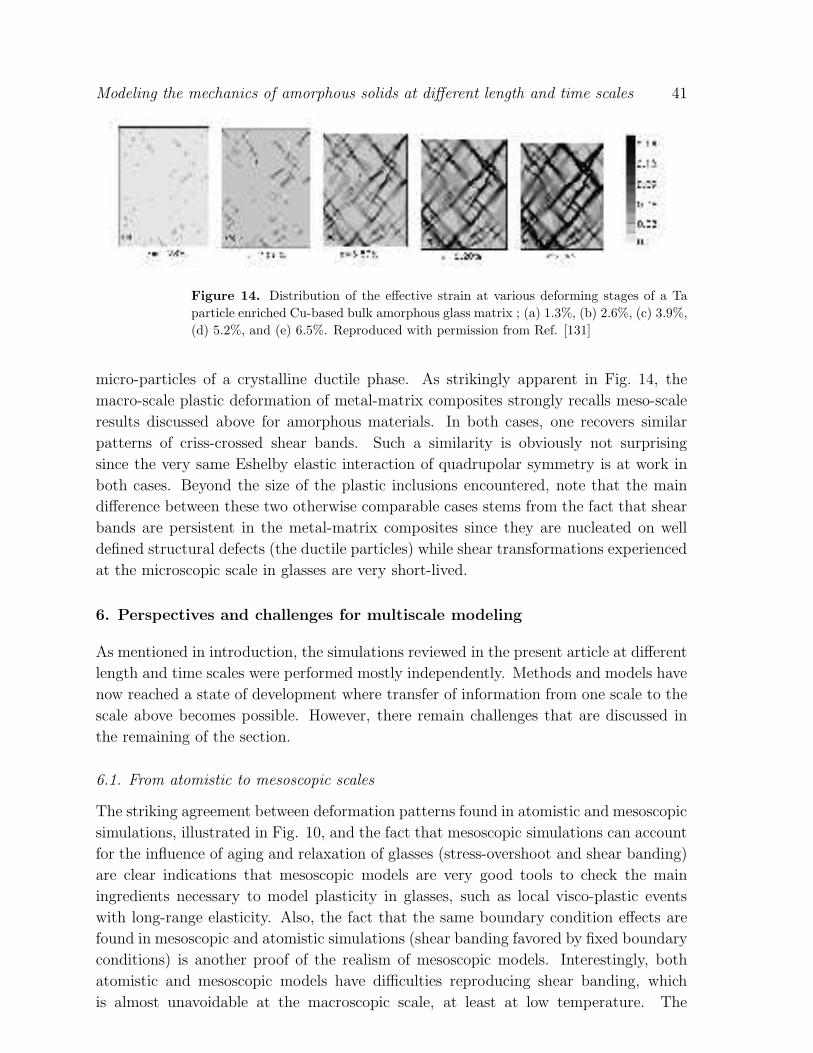
Modeling the mechanics of amorphous solids at different length and time scales 41
Figure 14. Distribution of the effective strain at various deforming stages of a Ta
particle enriched Cu-based bulk amorphous glass matrix ; (a) 1.3%, (b) 2.6%, (c) 3.9%,
(d) 5.2%, and (e) 6.5%. Reproduced with permission from Ref. [131]
micro-particles of a crystalline ductile phase. As strikingly apparent in Fig. 14, the
macro-scale plastic deformation of metal-matrix composites strongly recalls meso-scale
results discussed above for amorphous materials. In both cases, one recovers similar
patterns of criss-crossed shear bands. Such a similarity is obviously not surprising
since the very same Eshelby elastic interaction of quadrupolar symmetry is at work in
both cases. Beyond the size of the plastic inclusions encountered, note that the main
difference between these two otherwise comparable cases stems from the fact that shear
bands are persistent in the metal-matrix composites since they are nucleated on well
defined structural defects (the ductile particles) while shear transformations experienced
at the microscopic scale in glasses are very short-lived.
6. Perspectives and challenges for multiscale modeling
As mentioned in introduction, the simulations reviewed in the present article at different
length and time scales were performed mostly independently. Methods and models have
now reached a state of development where transfer of information from one scale to the
scale above becomes possible. However, there remain challenges that are discussed in
the remaining of the section.
6.1. From atomistic to mesoscopic scales
The striking agreement between deformation patterns found in atomistic and mesoscopic
simulations, illustrated in Fig. 10, and the fact that mesoscopic simulations can account
for the influence of aging and relaxation of glasses (stress-overshoot and shear banding)
are clear indications that mesoscopic models are very good tools to check the main
ingredients necessary to model plasticity in glasses, such as local visco-plastic events
with long-range elasticity. Also, the fact that the same boundary condition effects are
found in mesoscopic and atomistic simulations (shear banding favored by fixed boundary
conditions) is another proof of the realism of mesoscopic models. Interestingly, both
atomistic and mesoscopic models have difficulties reproducing shear banding, which
is almost unavoidable at the macroscopic scale, at least at low temperature. The
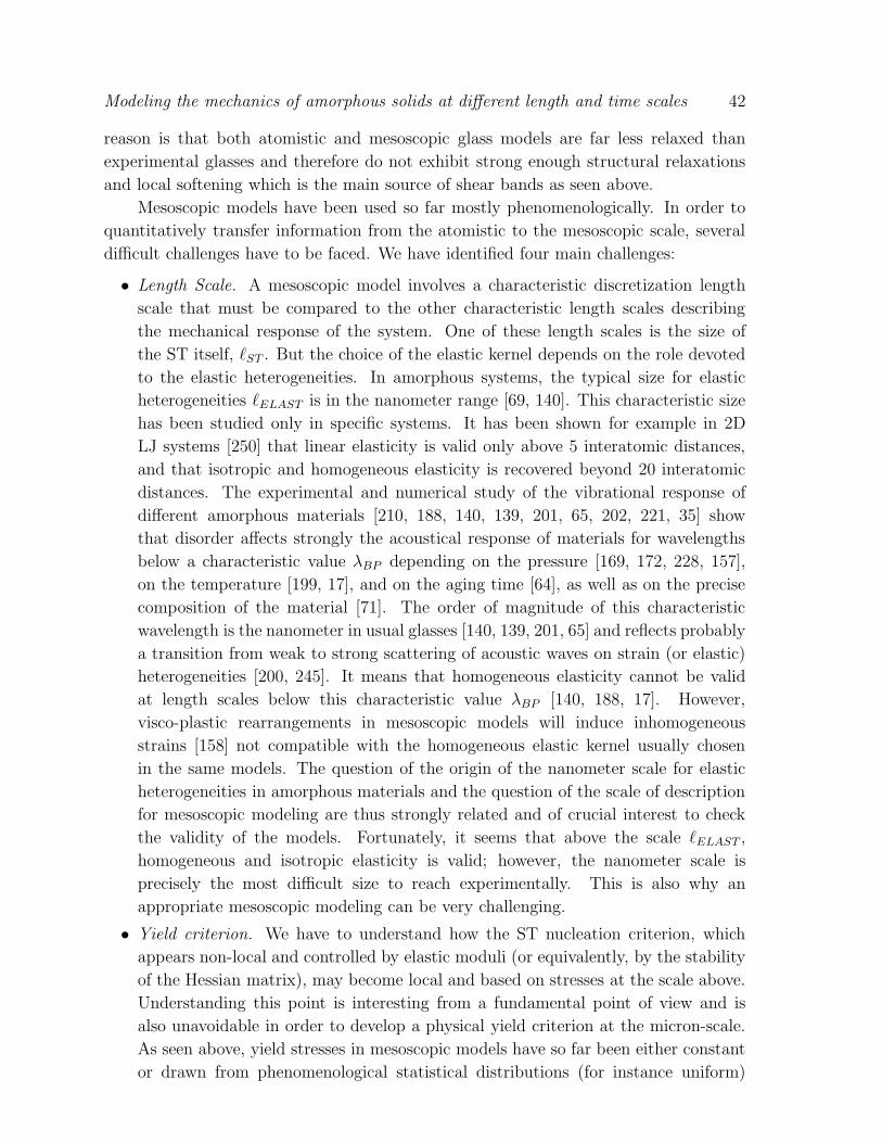
Modeling the mechanics of amorphous solids at different length and time scales 42
reason is that both atomistic and mesoscopic glass models are far less relaxed than
experimental glasses and therefore do not exhibit strong enough structural relaxations
and local softening which is the main source of shear bands as seen above.
Mesoscopic models have been used so far mostly phenomenologically. In order to
quantitatively transfer information from the atomistic to the mesoscopic scale, several
difficult challenges have to be faced. We have identified four main challenges:
• Length Scale. A mesoscopic model involves a characteristic discretization length
scale that must be compared to the other characteristic length scales describing
the mechanical response of the system. One of these length scales is the size of
the ST itself, ℓST . But the choice of the elastic kernel depends on the role devoted
to the elastic heterogeneities. In amorphous systems, the typical size for elastic
heterogeneities ℓELAST is in the nanometer range [69, 140]. This characteristic size
has been studied only in specific systems. It has been shown for example in 2D
LJ systems [250] that linear elasticity is valid only above 5 interatomic distances,
and that isotropic and homogeneous elasticity is recovered beyond 20 interatomic
distances. The experimental and numerical study of the vibrational response of
different amorphous materials [210, 188, 140, 139, 201, 65, 202, 221, 35] show
that disorder affects strongly the acoustical response of materials for wavelengths
below a characteristic value λBP depending on the pressure [169, 172, 228, 157],
on the temperature [199, 17], and on the aging time [64], as well as on the precise
composition of the material [71]. The order of magnitude of this characteristic
wavelength is the nanometer in usual glasses [140, 139, 201, 65] and reflects probably
a transition from weak to strong scattering of acoustic waves on strain (or elastic)
heterogeneities [200, 245]. It means that homogeneous elasticity cannot be valid
at length scales below this characteristic value λBP [140, 188, 17]. However,
visco-plastic rearrangements in mesoscopic models will induce inhomogeneous
strains [158] not compatible with the homogeneous elastic kernel usually chosen
in the same models. The question of the origin of the nanometer scale for elastic
heterogeneities in amorphous materials and the question of the scale of description
for mesoscopic modeling are thus strongly related and of crucial interest to check
the validity of the models. Fortunately, it seems that above the scale ℓELAST ,
homogeneous and isotropic elasticity is valid; however, the nanometer scale is
precisely the most difficult size to reach experimentally. This is also why an
appropriate mesoscopic modeling can be very challenging.
• Yield criterion. We have to understand how the ST nucleation criterion, which
appears non-local and controlled by elastic moduli (or equivalently, by the stability
of the Hessian matrix), may become local and based on stresses at the scale above.
Understanding this point is interesting from a fundamental point of view and is
also unavoidable in order to develop a physical yield criterion at the micron-scale.
As seen above, yield stresses in mesoscopic models have so far been either constant
or drawn from phenomenological statistical distributions (for instance uniform)
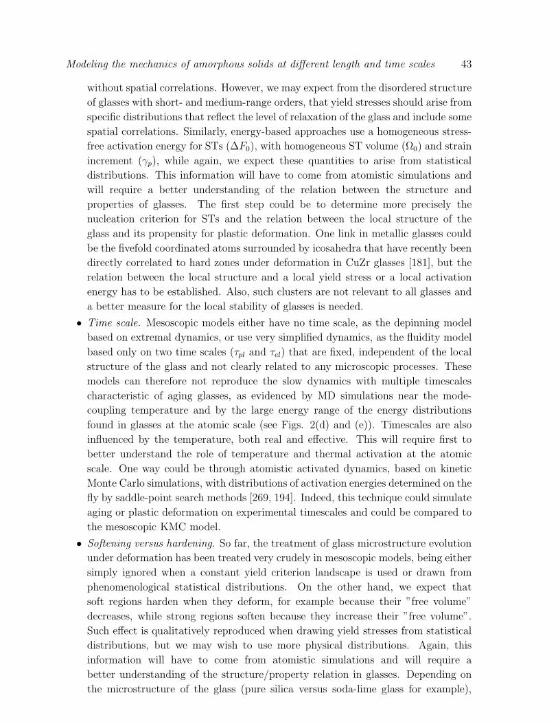
Modeling the mechanics of amorphous solids at different length and time scales 43
without spatial correlations. However, we may expect from the disordered structure
of glasses with short- and medium-range orders, that yield stresses should arise from
specific distributions that reflect the level of relaxation of the glass and include some
spatial correlations. Similarly, energy-based approaches use a homogeneous stress-
free activation energy for STs (∆F0), with homogeneous ST volume (Ω0) and strain
increment (γp), while again, we expect these quantities to arise from statistical
distributions. This information will have to come from atomistic simulations and
will require a better understanding of the relation between the structure and
properties of glasses. The first step could be to determine more precisely the
nucleation criterion for STs and the relation between the local structure of the
glass and its propensity for plastic deformation. One link in metallic glasses could
be the fivefold coordinated atoms surrounded by icosahedra that have recently been
directly correlated to hard zones under deformation in CuZr glasses [181], but the
relation between the local structure and a local yield stress or a local activation
energy has to be established. Also, such clusters are not relevant to all glasses and
a better measure for the local stability of glasses is needed.
• Time scale. Mesoscopic models either have no time scale, as the depinning model
based on extremal dynamics, or use very simplified dynamics, as the fluidity model
based only on two time scales (τpl and τel) that are fixed, independent of the local
structure of the glass and not clearly related to any microscopic processes. These
models can therefore not reproduce the slow dynamics with multiple timescales
characteristic of aging glasses, as evidenced by MD simulations near the mode-
coupling temperature and by the large energy range of the energy distributions
found in glasses at the atomic scale (see Figs. 2(d) and (e)). Timescales are also
influenced by the temperature, both real and effective. This will require first to
better understand the role of temperature and thermal activation at the atomic
scale. One way could be through atomistic activated dynamics, based on kinetic
Monte Carlo simulations, with distributions of activation energies determined on the
fly by saddle-point search methods [269, 194]. Indeed, this technique could simulate
aging or plastic deformation on experimental timescales and could be compared to
the mesoscopic KMC model.
• Softening versus hardening. So far, the treatment of glass microstructure evolution
under deformation has been treated very crudely in mesoscopic models, being either
simply ignored when a constant yield criterion landscape is used or drawn from
phenomenological statistical distributions. On the other hand, we expect that
soft regions harden when they deform, for example because their ”free volume”
decreases, while strong regions soften because they increase their ”free volume”.
Such effect is qualitatively reproduced when drawing yield stresses from statistical
distributions, but we may wish to use more physical distributions. Again, this
information will have to come from atomistic simulations and will require a
better understanding of the structure/property relation in glasses. Depending on
the microstructure of the glass (pure silica versus soda-lime glass for example),
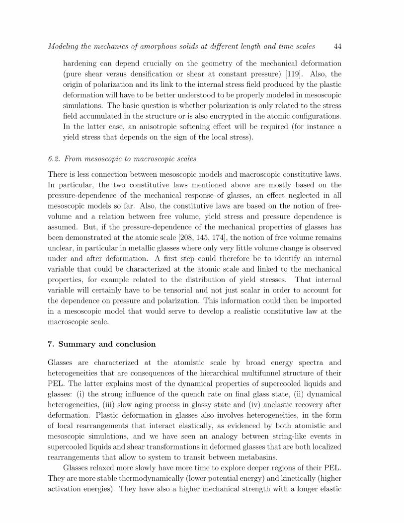
Modeling the mechanics of amorphous solids at different length and time scales 44
hardening can depend crucially on the geometry of the mechanical deformation
(pure shear versus densification or shear at constant pressure) [119]. Also, the
origin of polarization and its link to the internal stress field produced by the plastic
deformation will have to be better understood to be properly modeled in mesoscopic
simulations. The basic question is whether polarization is only related to the stress
field accumulated in the structure or is also encrypted in the atomic configurations.
In the latter case, an anisotropic softening effect will be required (for instance a
yield stress that depends on the sign of the local stress).
6.2. From mesoscopic to macroscopic scales
There is less connection between mesoscopic models and macroscopic constitutive laws.
In particular, the two constitutive laws mentioned above are mostly based on the
pressure-dependence of the mechanical response of glasses, an effect neglected in all
mesoscopic models so far. Also, the constitutive laws are based on the notion of free-
volume and a relation between free volume, yield stress and pressure dependence is
assumed. But, if the pressure-dependence of the mechanical properties of glasses has
been demonstrated at the atomic scale [208, 145, 174], the notion of free volume remains
unclear, in particular in metallic glasses where only very little volume change is observed
under and after deformation. A first step could therefore be to identify an internal
variable that could be characterized at the atomic scale and linked to the mechanical
properties, for example related to the distribution of yield stresses. That internal
variable will certainly have to be tensorial and not just scalar in order to account for
the dependence on pressure and polarization. This information could then be imported
in a mesoscopic model that would serve to develop a realistic constitutive law at the
macroscopic scale.
7. Summary and conclusion
Glasses are characterized at the atomistic scale by broad energy spectra and
heterogeneities that are consequences of the hierarchical multifunnel structure of their
PEL. The latter explains most of the dynamical properties of supercooled liquids and
glasses: (i) the strong influence of the quench rate on final glass state, (ii) dynamical
heterogeneities, (iii) slow aging process in glassy state and (iv) anelastic recovery after
deformation. Plastic deformation in glasses also involves heterogeneities, in the form
of local rearrangements that interact elastically, as evidenced by both atomistic and
mesoscopic simulations, and we have seen an analogy between string-like events in
supercooled liquids and shear transformations in deformed glasses that are both localized
rearrangements that allow to system to transit between metabasins.
Glasses relaxed more slowly have more time to explore deeper regions of their PEL.
They are more stable thermodynamically (lower potential energy) and kinetically (higher
activation energies). They have also a higher mechanical strength with a longer elastic
Modeling the mechanics of amorphous solids at different length and time scales 45
regime and larger elastic moduli. These effects arise naturally in atomistic simulations
and are reproduced phenomenologically in mesoscopic models, for instance by increasing
the initial level of yield stresses. However, a more quantitative description of this effect
at the micron scale is still lacking, because it requires a deeper understanding of the
dynamics of relaxation and aging in glasses. This is related to a better understanding of
the dissipative processes at small scale that are far to be understood in general, as soon
as they involve electron-phonon couplings. Moreover, the effect of bond directionality,
already known in crystalline plasticity, is far from being quantitatively understood,
as well as the corresponding relation between local structure and plastic damage in
amorphous materials, and eventually its mesoscopic description.
Instabilities in the plastic regime are observed at all scales and depend on the
way the simulations are carried out. The simplest models, both at the atomistic
and mesoscopic scales, do not lead to persistent shear bands. Indeed, in atomistic
simulations, unless slow quench rates on MD timescales are used to prepare glasses, or
strong interatomic bond directionality, the glass will only undergo transient localizations
in the form of elementary shear bands. Similarly, at the mesoscale, we have seen that
correlations and disorder can have different origins (dynamical and structural) and that
a model without softening, i.e. without structural correlations, but with structural
disorder (initial distribution of internal stresses or with stochastic yield stresses) show
transient localization patterns, but no permanent shear bands. The other condition
to form shear bands is when the glass contains no structural disorder, which explains
the strain rate effect of shear banding: shear bands form only when the strain rate
is slow enough that the rate of production of structural disorder (which increase with
the strain rate) is slower than the relaxation rate of structural disorder. Shear bands
are observed in relaxed glasses that exhibit softening, which requires to apply a slow
quench at atomistic scale or to include softening effects at the mesoscopic scale. Another
way to generate permanent shear bands is to run simulations on covalent systems
with strong three-body interactions (bond directionality) at low pressure, because a
constant pressure contributes to homogenize the deformation. A better understanding
of softening and relaxations at the atomistic and meso-scales is a major issue, which
requires to better understand the physics of STs (their nucleation criterion and relation
to local softening or hardening). At the macroscopic scale, softening can be included
in constitutive laws but the question is what is the relevant internal variable and
its corresponding dynamics to represent faithfully the dynamics of STs and of their
interactions and relation to softening. At the macroscopic scale, reproducing history-
dependence may require to generalize the notions of effective temperature and free
volume to transform them into tensorial quantities to reproduce anisotropy and the fact
that the symmetry of the plastic strain tensor gets embedded in glass microstructure,
leading to anelasticity. Less-relaxed glasses that present a larger density of nucleation
sites for plasticity (although the nature of these sites remains elusive, as discussed above)
have a lower strength but a higher ductility. This observation is at the basis of several
strategies to produce ductile metallic glasses, such as prestraining [274, 132] or ion
Modeling the mechanics of amorphous solids at different length and time scales 46
irradiation [189].
Finally, the question of the temperature dependence of the mechanical response
is still largely an open question. Different regimes have been explored, especially the
athermal regime and the mean-field regime at higher temperatures. But a relevant
description of thermal processes and their competition with mechanical instabilities
needs a deeper understanding of the evolution of activation barriers and memory
effects in mechanically driven systems and the question of the competition between the
dynamics of the numerically chosen thermostat and the local dynamics of the mechanical
instabilities makes this question difficult to solve at the moment.
We end with a few open questions that we deem important to answer in order
to make significant progress. At the atomic scale, can we identify a geometrical
characteristic of weak zones in metallic glasses, more general than coordination defects
or special structural environments like icosahedra? Related to temperature, is it possible
to quantify properly the respective nucleation and diffusion from a nucleated center of
plastic rearrangements? How does the size of the plastic rearrangements depend on
the shear rate? What is responsible for the nucleation of large scale rearrangements
like elementary shear bands, and do these large scale rearrangements resist thermal
activation? Do these large scale events imply non-uniform temperatures, and local
melting that would favor crack propagation? What are the characteristic timescales for
structural and mechanical relaxations that must be included in mesoscopic models? All
these questions need a more realistic description of the local dissipative processes, that
are strongly system-dependent. At the mesoscale, is it possible to find a characteristic
length scale for self-consistent mesoscopic models? Which internal variable will account
for the specific microscopic structure of the system (for instance, bond directionality),
and corresponding relaxations? At the macro-scale, is it possible to derive a general
constitutive law from microscopic modeling that can take into account the competition
between shear and densification, with a complete description of the mechanical history?
How does it depend on the specific composition of a glass? The above questions are
but a few among a vast list of topics for future research that will benefit from the
continuous progress in simulation techniques and experiments, and will hopefully lead
to a general understanding and description of glassy mechanics consistent across length-
and time-scales.
8. References
[1] F. Albano and M.L. Falk. Shear softening and structure in a simulated three-dimensional binary
glass. J. Chem. Phys., 122:154508, 2005.
[2] M.P. Allen and D. Tildesley. Computer simulation of liquids. Clarendon Press, Oxford, 1987.
[3] L. Anand and D. Hennann. A constitutive theory for the mechanical response of amorphous
metals at high temepratures spanning the glass transition temperature: application to
microscale thermoplastic forming. Acta Mater., 56:3290–3305, 2008.
[4] L. Anand and C. Su. A theory for amorphous viscoplastic materials undergoing finite
deformations, with application to metallic glasses. J. Mech. Phys. Solids, 53:1362–1396, 2005.
Modeling the mechanics of amorphous solids at different length and time scales 47
[5] L. Anand and C. Su. A constitutive theory for metallic glasses at high homologous temperatures.
Acta Mater., 55:3735–3747, 2007.
[6] L. Angelani, R. Di Leonardo, G. Ruocco, A. Scala, and F. Sciortino. Saddles in the energy
landscape probed by supercooled liquids. Phys. Rev. Lett., 85:5356–5359, 2000.
[7] L. Angelani, G. Parisi, G. Ruocco, and G. Viliani. Potential energy landscape and long-time
dynamics in a simple model glass. Phys. Rev. E, 61:1681–1691, 2000.
[8] G.A. Appignanesi, J.A. Rodriguez Fris, R.A. Montani, and W. Kob. Democratic particle motion
for metabasin transitions in simple glass formers. Phys. Rev. Lett., 96:057801, 2006.
[9] A.S. Argon. Delayed elasticity in inorganic glasses. J. Appl. Phys., 39:4080–4086, 1968.
[10] A.S. Argon. Plastic deformation in metallic glasses. Acta Metall., 27:47–58, 1979.
[11] A.S. Argon and H.Y. Kuo. Plastic flow in a disordered bubble raft. Mat. Sci. Eng., 39:101–109,
1979.
[12] A.S. Argon and H.Y. Kuo. Free energy spectra for inelastic deformation of five metallic glass
alloys. J. Non-Cryst. Sol., 37:241–266, 1980.
[13] M.F. Ashby and A.L. Greer. Metallic glasses as structural materials. Scripta Mat., 54:321–326,
2006.
[14] D. Bacon, Y. Osetsky, and D. Rodney. Dislocation-obstacle interactions at the atomic level.
In J. Hirth and L. Kubin, editors, Dislocations in Solids, volume 15, chapter 88, pages 1–90.
Elsevier, 2009.
[15] N.P. Bailey, J. Schiotz, and K.W. Jacobsen. Simulation of cu-mg metallic glass: Thermodynamics
and structure. Phys. Rev. B, 69:144205, 2004.
[16] N.P. Bailey, J. Schiotz, A. Lemaıtre, and K.W. Jacobsen. Avalanche size scaling in sheared
three-dimensional amorphous solid. Phys. Rev. Lett., 98:095501, 2007.
[17] G. Baldi, A. Fontana, G. Monaco, L. Orsingher, S. Rols, F. Rossi, and B. Ruta. Connection
between the boson peak and elastic properties in silicate glasses. Phys. Rev. Lett., 102:195502,
2009.
[18] J.-C. Baret, D. Vandembroucq, and S. Roux. An extremal model of amorphous plasticity. Phys.
Rev. Lett., 89:195506, 2002.
[19] J.L Barrat and A. Lemaıtre. Heterogeneities in amorphous systems under shear. In L. Berthier,
G. Biroli, J.P. Bouchaud, L. Cipelletti, andW. van Saarloos, editors, Dynamical Heterogeneities
in Glasses, Colloids, and Granular Media. Oxford University Press, 2010.
[20] M.Z. Bazant and E. Kaxiras. Modeling of covalent bonding in solids by inversion of cohesive
energy curves. Phys. Rev. Lett., 77:4370–4373, 1996.
[21] M.Z. Bazant, E. Kaxiras, and J.F. Justo. Environment-dependent interatomic potential for bulk
silicon. Phys. Rev. B, 56:8542–8552, 1997.
[22] L. Berthier and J.L. Barrat. Nonequilibrium dynamics and fluctuation-dissipation relation in a
sheared fluid. J. Chem. Phys., 116:6228–6242, 2002.
[23] L. Berthier and J.L. Barrat. Shearing a glassy material: numerical test of nonequilibrium mode-
coupling approaches and experimental proposals. Phys. Rev. Lett., 89:095702, 2002.
[24] L. Berthier and G. Biroli. A theoretical perspective on the glass transition and nonequilibrium
phenomena in disordered materials. arxiv:1011.2578, 2010.
[25] K. Binder and W. Kob. Glassy materials and disordered solids: an introduction to their statistical
mechanics. World Scientific, Singapore, 2005.
[26] L. Bocquet and A. Ajdari. Kinetic theory of plastic flow in soft glassy materials. Phys. Rev.
Lett., 103:036001, 2009.
[27] D. Bonamy. Intermittency and roughening in the failure of brittle heterogeneous materials. J.
Phys. D, 42:2114014, 2009.
[28] K. Broderix, K.K. Bhattacharya, A. Cavagna, A. Zippelius, and I. Giardina. Energy landscape
of a lennard-jones liquid: statistics of stationary points. Phys. Rev. Lett., 85:5360–5364, 2000.
[29] S. Buchner and A. Heuer. Metastable states as a key to the dynamics of the supercooled liquids.
Phys. Rev. Lett., 84:2168–2171, 2000.
Modeling the mechanics of amorphous solids at different length and time scales 48
[30] V. V. Bulatov and A. S. Argon. A stochastic model for continuum elasto-plastic behavior. I.
numerical approach and strain localization. Model. Simul. Mater. Sci. Eng., 2:167, 1994.
[31] V. V. Bulatov and A. S. Argon. A stochastic model for continuum elasto-plastic behavior. II. a
study of the glass transition and structural relaxation. Model. Simul. Mater. Sci. Eng., 2:185,
1994.
[32] V. V. Bulatov and A. S. Argon. A stochastic model for continuum elasto-plastic behavior. III.
plasticity in ordered versus disordered solids. Model. Simul. Mater. Sci. Eng., 2:203, 1994.
[33] E. Cances, F. Legoll, M.C. Marinica, K. Minoukadeh, and F. Willaime. Some improvements of
the activation-relaxation technique method for finding transition pathways on potential energy
surfaces. J. Chem. Phys., 130:114711, 2009.
[34] A. Carr, J. Horbach, S. Ispas, and W. Kob. New fitting scheme to obtain effective potential
from car-parrinello molecular dynamics simulations: application to silica. Eur. Phys. Lett.,
82:17001, 2008.
[35] B. Champagnon, L. Wondraczek, and T. Deschamps. Boson peak, structural inhomogeneity,
light scattering and transparency of silicate glasses. J. Non-Cryst. Sol., 355:712, 2009.
[36] L. Charleux, S. Gravier, M. Verdier, M. Fivel, and J.J. Blandin. Indentation plasticity of
amorphous and partially crystallized metallic glasses. J. Mater. Res., 22:525–532, 2006.
[37] J. Chattoraj, C. Caroli, and A. Lemaıtre. Universal, additive effect of temperature on the rheology
of amorphous solids. Phys. Rev. Lett., 105:266001, 2010.
[38] G.L. Chen, X.J. Liu, X.D. Hui, H.K. Hou, K.F. Yao, C.T. Liu, and J. Wadsworth. Molecular
dynamic simulations and atomic structures of amorphous materials. Appl. Phys. Lett.,
88:203115, 2006.
[39] Y.Q. Cheng, A.J. Cao, and E. Ma. Correlation between the elastic modulus and the intrinsic
plastic behavior of metallic glasses: the roles of atomic configuration and alloy composition.
Acta Mater., 57:3253–3267, 2009.
[40] Y.Q. Cheng, A.J. Cao, H.W. Sheng, and E. Ma. Local order influences initiation of plastic
flow in metallic glass: effect of alloy composition and sample cooling history. Acta Mater.,
56:5263–5275, 2008.
[41] M. Cloitre, R. Borrega, F. Monti, and L. Leibler. Glassy dynamics and flow properties of soft
colloidal pastes. Phys. Rev. Lett., 90:068303, 2003.
[42] D. Coslovich and G. Pastore. Understanding fragility in supercooled lennard-jones mixtures. i.
locally preferred structures. J. Chem. Phys., 127:124504, 2007.
[43] P. Coussot and J.L. Grossiord, editors. Understanding rheology - From blood circulation to
concrete hardening, Paris, 2002. EDP Sciences.
[44] P. Coussot and G. Ovarlez. Physical origin of shear-banding in jammed systems. Eur. Phys. J.
E, 33:183–188, 2010.
[45] P. Coussot, J.S. Raynaud, F. Bertrand, P. Moucheront, J.P. Guilbaud, H.T. Huynh, S. Jarny,
and D. Lesueur. Coexistence of liquid and solid phases in flowing soft-glassy materials. Phys.
Rev. Lett., 88:218301, 2002.
[46] L.F. Cugliandolo, J. Kurchan, and L. Peliti. Energy flow, partial equilibration, and effective
temperatures in systems with slow dynamics. Phys. Rev. E, 55:3898–3914, 1997.
[47] K. Dahmen, D. Ertas, and Y. Ben-Zion. Gutemberg-richter and characteristic earthquake
behavior insimple-mean-field models of heterogeneous faults. Phys. Rev. E, 58:1494–1501,
1998.
[48] K. A. Dahmen, Y. Ben-Zion, and J. T. Uhl. Micromechanical model for deformation in solids with
universal predictions for stress-strain curves and slip avalanches. Phys. Rev. Lett., 102:175501,
2009.
[49] A.M.R. de Graff and M.F. Thorpe. The long-wavelength limit of the structure factor of
amorphous silicon and vitreous silica. Acta Cryst., A66:22, 2010.
[50] P.G. Debenedetti and F.H. Stillinger. Supercooled liquids and the glass transition. Nature,
410:259–267, 2001.
Modeling the mechanics of amorphous solids at different length and time scales 49
[51] F. Delogu. Indentification and characterization of potential shear transformation zones in metallic
glasses. Phys. Rev. Lett., 100:255901, 2008.
[52] M.J. Demkowicz and A.S. Argon. High-density liquidlike component facilitates plastic flow in a
model amorphous silicon system. Phys. Rev. Lett., 93:025505, 2004.
[53] M.J. Demkowicz and A.S. Argon. Autocatalytic avalanches of unit inelastic shearing events are
the mechanism of plastic deformation in amorphous silicon. Phys. Rev. B, 72:245206, 2005.
[54] R.A. Denny, D.R. Reichman, and J.P. Bouchaud. Trap model and slow dynamics in supercooled
liquids. Phys. Rev. Lett., 90:025503, 2003.
[55] B. Devincre, T. Hoc, and L. Kubin. Dislocation mean free paths and strain hardening of crystals.
Science, 320:1745–1748, 2008.
[56] D.M. Dimiduk, C. Woodward, and R. LeSarand M.D. Uchic. Scale free intermittent flow in
crystal plasticity. Science, 26:1188–1190, 2006.
[57] B. Doliwa and A. Heuer. Energy barriers and activated dynamics in a supercooled lennard-jones
liquid. Phys. Rev. E, 67:031506, 2003.
[58] B. Doliwa and A. Heuer. Hopping in a supercooled lennard-jones liquid: metabasins, waiting
time distribution, and diffusion. Phys. Rev. E, 67:030501, 2003.
[59] B. Doliwa and A. Heuer. What does the potential energy landscape tell us about the dynamics
of supercooled liquids and glasses? Phys. Rev. Lett., 91:235501, 2003.
[60] C. Donati, J.F. Douglas, W. Kob, S.J. Plimpton, P.H. Poole, and S.C. Glotzer. Stringlike
cooperative motion in a supercooled liquid. Phys. Rev. Lett., 80:2338–2342, 1998.
[61] C.D. Donati, S.C. Glotzer, P.H. Poole, W. Kob, and S.J. Plimpton. Spatial correlations of
mobility and immobility in a glass-forming lennard-jones liquid. Phys. Rev. E, 60:3107, 1999.
[62] J.P.K. Doye and D.J. Wales. Saddle points and dynamics of lennard-jones clusters, solids and
supercooled liquids. J. Chem. Phys., 116:3777–3788, 2002.
[63] G. Duan, D. Xu, Q. Zhang, G. Zhang, T. Cagin, W.L. Johnson, and W.A. Goddard III.
Molecular dynamics study of the binary cu46zr54 metallic glass motivated by experiments:
Glass formation and atomic-level structure. Phys. Rev. B, 71:224208, 2005.
[64] A. Duval, S. Etienne, G. Simeoni, and A. Mermet. Physical aging effect on the boson peak and
heterogeneous nanostructure of a silicate glass. J. Non-Cryst. Sol., 352:4525, 2006.
[65] A. Duval, A. Mermet, and L. Saviot. Boson peak and hybridization of acoustic modes with
vibrations of nanometric heterogeneities in glasses. Phys. Rev. B, 75:024201, 2007.
[66] J.C. Dyre. Master-equation approach to the glass transition. Phys. Rev. Lett., 58:792–795, 1987.
[67] M.D. Ediger, C.A. Angell, and S.R. Nagel. Supercooled liquids and glasses. J. Chem. Phys.,
100:13200–13212, 1996.
[68] T. Egami, W. Dmowski, P. Kosmetatos, M. Boord, T. Tomida, E. Oikawa, and A. Inoue.
Deformation induced bond orientational order in metallic glasses. J. Non-Cryst. Sol.,
192&193:591–594, 1995.
[69] H. Ehmler, A. Heesemann, K. Ratzke, and F. Faupel. Mass dependence of diffusion in a
supercooled metallic melt. Phys. Rev. Lett., 80:4919–4922, 1998.
[70] J. D. Eshelby. The determination of the elastic field of an ellipsoidal inclusion, and related
problems. Proc. Roy. Soc. A, 241:376, 1957.
[71] E. Fabiani, A. Fontana, and U. Buchenau. Neutron scattering study of the vibrations in silica
and germania. J. Chem. Phys., 128:244507, 2008.
[72] M.L. Falk and J.S. Langer. Dynamics of viscoplastic deformation in amorphous solids. Phys.
Rev. E, 57:7192–7205, 1998.
[73] M.L. Falk and C.E. Maloney. Simulating the mechanical response of amorphous solids using
atomistic methods. Eur. Phys. J. B, 75:405–413, 2010.
[74] S. M. Fielding, M. E. Cates, and P. Sollich. Shear banding, aging and noise dynamics in soft
glassy materials. Soft Matter, 5:2378–2382, 2009.
[75] D. S. Fisher, K. Dahmen, and Y. Ben-Zion. Statistics of earthquakes in simple models of
heterogeneous faults. Phys. Rev. Lett., 78:4885–4888, 1997.
Modeling the mechanics of amorphous solids at different length and time scales 50
[76] K. M Flores and R. H. Dauskardt. Mean stress effects on flow localization and failure in a bulk
metallic glass. Acta Mater., 49:2527–2537, 2001.
[77] D. Frenkel and B. Smith. Understanding molecular simulation: from algorithms to applications.
Academic Press, San Diego, 2002.
[78] C. Fusco, T. Albaret, and A. Tanguy. Role of local order in the small-scale plasticity of model
amorphous materials. Phys. Rev. E, 82:066116, 2010.
[79] P. Ganesh and M. Widom. Signature of nearly icosahedral structures in liquid and supercooled
liquid copper. Phys. Rev. B, 74:134205, 2006.
[80] P. Ganesh and M. Widom. Ab initio simulations of geometrical frustration in supercooled liquid
fe and fe-based metallic glass. Phys. Rev. B, 77:014205, 2008.
[81] Y. F. Gao. An implicit finite element method for simulating inhomogeneous deformation and
shear bands of amorphous alloys based on the free-volume model. Model. Simul. Mater. Sci.
Eng., 14:1329–1345, 2006.
[82] Y. F. Gao and A. F. Bower. A simple technique for avoiding convergebce problem in finite element
simulations of crack nucleation and growth on cohesive interfaces. Model. Simul. Mater. Sci.
Eng., 12:453–463, 2006.
[83] J. Godet, L. Pizzagalli, S. Brochard, and P. Beauchamp. Comparison between classical potentials
and ab initio moethods for silicon under large shear. J. Phys.: Cond. Mat., 15:6943–6953, 2003.
[84] M. Goldstein. Viscous liquids and the glass transition: a potential energy barrier picture. J.
Chem. Phys., 51:3728–3739, 1969.
[85] W. Gotze and L. Sjogren. Relaxation processes in supercooled liquids. Rep. Prog. Phys., 55:241–
376, 1992.
[86] X.J. Gu, S.J. Poon, G.J. Shiflet, and M. Widom. Mechanical properties, glass transition
temperature, and bond enthalpy trends of high metalloid fe-based bulk metallic glasses. Appl.
Phys. Lett., 92:161910, 2008.
[87] J. Guckenheimer and P. Homes. Nonlinear oscillations, dynamical systems, and bifurcation of
vector fields, 3rd Ed. Springer-Verlag, New York, 1997.
[88] X.J. Han and H. Teichler. Liquid-to-glass transition in bulk glass-forming cu60ti20zr20 alloy by
molecular dynamics simulations. Phys. Rev. E, 75:061501, 2007.
[89] J.S. Harmon, M.D. Demetriou, W.L. Johnson, and K. Samwer. Anelastic to plastic transition in
metallic glass-forming liquids. Phys. Rev. Lett., 99:135502, 2007.
[90] J.A. Hauch, D. Holland, M.P. Marder, and H.L. Swinney. Dynamic fracture in single crystal
silicon. Phys. Rev. Lett., 82:3823–3826, 1999.
[91] T.K. Haxton and A.J. Liu. Activated dynamics and effective temperature in a steady state
sheared glass. Phys. Rev. Lett., 99:195701, 2007.
[92] P. Hebraud and F. Lequeux. Mode-coupling theory for the pasty rheology of soft glassy materials.
Phys. Rev. Lett., 81:2934–2937, 1998.
[93] M. Heilmaier. Deformation behavior of zr-based metllic glasses. J. Mat. Proc. Tech., 117:374–
380, 2001.
[94] W.H. Herschel and R. Bulkley. Konsistenzmessungen von gummi-benzollosungen. Kolloid
Zeitschrift, 39:291, 1926.
[95] A. Heuer. Properties of a glass-forming system as derived from its potential energy landscape.
Phys. Rev. Lett., 78:4051–4055, 1997.
[96] A. Heuer. Exploring the potential energy landscape of glass-forming systems: from inherent
structures via metabasins to macroscopic transport. J. Phys.: Cond. Mat., 20:373101, 2008.
[97] J.P. Hirth and J. Lothe. Theory of dislocations. Wiley, New York, 1982.
[98] E.R. Homer, D. Rodney, and C.A. Schuh. Kinetic monte carlo study of activated states and
correlated shear-transformation-zone activity during the deformation of an amorphous metal.
Phys. Rev. E, 81:064204, 2010.
[99] E.R. Homer and C.A. Schuh. Mesoscale modeling of amorphous metals by shear transformation
zone dynamics. Acta Mater., 57:2823–2833, 2009.
Modeling the mechanics of amorphous solids at different length and time scales 51
[100] E.R. Homer and C.A. Schuh. Three-dimensional shear transformation zone dynamics model for
amorphous metals. Model. Simul. Mater. Sci. Eng., 18:065009, 2010.
[101] L. Huang and J. Kieffer. Molecular dynamics study of cristobalite silica using a charge transfer
three-body potential: phase transformation and structural disorder. J. Chem. Phys., 118:1487–
1498, 2003.
[102] R. Huang, Z. Suo, J. H. Prevost, and W. D. Nix. Inhomogeneous deformation in metallic glasses.
J. Mech. Phys. Solids, 50:1011–1027, 2002.
[103] P. Ilg and J.L. Barrat. Driven activation vs. thermal activation. Eur. Phys. Lett., 79:26001,
2007.
[104] A. Inoue. Stabilization of metallic supercooled liquid and bulk amorphous alloys. Acta Mater.,
48:279–306, 2000.
[105] S. Ispas, M. Benoit, P. Jund, and R. Jullien. Structural properties of glassy and liquid
tetrasilicate, comparison between ab initio and classical molecular-dynamics simulations. J.
Non-Cryst. Sol., 307-310:946–955, 2002.
[106] S. Ispas, N. Zotov, S. de Wispaleare, and W. Kob. Vibrational properties of a sodium tetrasilicate
glass: ab initio versus classical force field. J. Non-Cryst. Sol., 351:1144–1150, 2005.
[107] E. A. Jagla. Strain localization driven by structural relaxation in sheared amorphous solids.
Phys. Rev. E, 76:046119, 2007.
[108] N. Jakse and A. Pasturel. Local order of liquid and supercooled zirconium by ab initio molecular
dynamics. Phys. Rev. Lett., 91:195501, 2003.
[109] Hui Ji, V. Keryvin, T. Rouxel, and T. Hammouda. Densification of window glass under very
high pressure and its relevance to vickers indentation. Scripta Mat., 55:1159–1162, 2006.
[110] G.P. Johari and M. Goldstein. Viscous liquids and the glass transition. ii. secondary relaxations
in glasses of rigid molecules. J. Chem. Phys., 53:2372–2389, 1970.
[111] W.L. Johnson. Bulk glass-forming metallic alloys: science and technology. Mater. Res. Soc.
Bull., 24:42–56, 1999.
[112] W.L. Johnson and K. Samwer. A universal criterion for plastic yielding of metallic glasses with
a (t/tg)3/2 temperature dependence. Phys. Rev. Lett., 95:1995501, 2005.
[113] H. Jonsson and H.C. Andersen. Isosahedral ordering in the lennard-jones liquid and glass. Phys.
Rev. Lett., 60:2295–2298, 1988.
[114] M. Kardar. Nonequilibrium dynamics of interfaces and lines. Phys. Rep., 301:85–112, 1998.
[115] S. Karmakar, E. Lerner, and I. Procaccia. Statistical physics of elasto-plastic steady states in
amorphous solids. Phys. Rev. E, 82:055103, 2010.
[116] Y. Kawamura and A. Inoue. Newtonian viscosity of supercooled liquid in a pd40ni40p20 metallic
glass. Appl. Phys. Lett., 76:1114–1116, 2001.
[117] T. Kawasaki, T. Araki, and H. Tanaka. Correlation between dynamic heterogeneity and medium-
range order in two-dimensional glass-forming liquids. Phys. Rev. Lett., 99:215701, 2007.
[118] V.Y. Kazimirov, D. Louca, M. Widom, X.J. Gu, S.J. Poon, and G.J. Shiflet. Local organization
and atomic clustering in multicomponent amorphous steels. Phys. Rev. B, 78:054112, 2008.
[119] G. Kermouche, E. Barthel, D. Vandembroucq, and P. Dubujet. Mechanical modelling of
indentation-induced densification in amorphous silica. Acta Mater., 56:3222–3228, 2008.
[120] V. Khonik, Y.P. Mitrofanov, S.A. Lyakhov, D.A. Khoviv, and R.A. Kouchakov. Recovery
of structural relaxation in aged metallic glass as determined by high-precision in situ shear
modulus measurements. J. Appl. Phys., 105:123521, 2009.
[121] W. Klement, R.H. Willens, and P. Duwez. Noncrystalline structure in solidified gold-silicon
alloys. Nature, 187:869–870, 1960.
[122] W. Kob and H.C. Andersen. Testing mode-coupling theory for a supercooled binary lennard-jones
mixture: the van hove correlation function. Phys. Rev. E, 51:4626–4641, 1995.
[123] W. Kob, C. Donati, S.J. Plimpton, P.H. Poole, and S.C. Glotzer. Dynamical heterogeneities in
a supercooled lennard-jones liquid. Phys. Rev. Lett., 79:2827–2831, 1997.
[124] S. Kobayashi, K. Maeda, and S. Takeuchi. Computer simulation of atomic structure of cu57zr43
Modeling the mechanics of amorphous solids at different length and time scales 52
amorphous alloy. J. Phys. Soc. Japan, 48:1147–1152, 1980.
[125] S. Kobayashi, K. Maeda, and S. Takeuchi. Computer simulation of deformation of amorphous
cu57zr43. Acta Metall., 28:1641–1652, 1980.
[126] A. Kushima, X. Lin, J. Li, J. Eapen, J.C. Mauro, X. Qian, P. Diep, and S. Yip. Computing the
viscosity of supercooled liquids. J. Chem. Phys., 130:224504, 2009.
[127] D.J. Lacks. Energy landscape and the non-newtonian viscoity of liquids and glasses. Phys. Rev.
Lett., 87:225502, 2001.
[128] J. C. Lambropoulos, S. Xu, and T. Fang. Constitutive law for the densification of fused silica,
with applications in polishing and microgrinding. J. Am. Ceram. Soc., 79:1441–1452, 1996.
[129] F. Lancon, L. Billard, and P. Chaudhari. Thermodynamical properties of a two-dimensional
quasicrystal from molecular dynamics calculations. Europhys. Lett., 2:625–629, 1986.
[130] J. Lauridsen, G. Chanan, and M. Dennin. Velocity profiles in slowly sheared bubble rafts. Phys.
Rev. Lett., 93:018303, 2004.
[131] J. C. Lee, Y. C. Kim, J. P. Ahn, and H. S. Kim. Enhanced plasticity in bulk amorphous matrix
composites: macroscopic and microscopic viewpoint studies. Acta Mater., 53:129–139, 2005.
[132] S.C. Lee, C.M. Lee, J.W. Yang, and J.C. Lee. Microstructural evolution of an elastostatically
compressed amorphous alloy and its influence on the mechanical properties. Scripta Mat.,
58:591–594, 2008.
[133] A. Lemaıtre and C. Caroli. Rate-dependent avalanche size in athermally sheared amorphous
solids. Phys. Rev. Lett., 065501:2009, 103.
[134] A. Lemaıtre and C. Caroli. Dynamical noise and avalanches in quasi-static flow of amorphous
materials. arxiv:0609689v1, 2006.
[135] A. Lemaıtre and C. Caroli. Plastic response of a two-dimensional amorphous solid to quasistatic
shear: transverse particle diffusion and phenomenology of dissipative events. Phys. Rev. E,
76:036104, 2007.
[136] A. Lemaıtre and C. Caroli. Plastic response of a two-dimensional amorphous solid to quasistatic
shear: Transverse particle diffusion and phenomenology of dissipative events. Phys. Rev. E,
76:036104, 2007.
[137] F. Leonforte. Vibrations et micromecanique de materiaux amorphes modeles. PhD thesis,
Universite Lyon 1, 2006.
[138] F. Leonforte, R. Boissiere, A. Tanguy, J. P. Wittmer, and J.-L. Barrat. Continuum limit of
amorphous elastic bodies iii: three-dimensional systems. Phys. Rev. B, 72:224206, 2005.
[139] F. Leonforte, A. Tanguy, and J.-L. Barrat. Inhomogeneous elastic response of silica glass. Phys.
Rev. Lett., 97:055501, 2006.
[140] F. Leonforte, A. Tanguy, J. P. Wittmer, and J.-L. Barrat. Continuum limit of amorphous elastic
bodies i: a finite-size study of low-frequency harmonic vibrations. Phys. Rev. B, 66:174205,
2002.
[141] H. Leschhorn, T. Nattermann, S. Stepanow, and L.H. Tang. Driven interface depinning in a
disordered medium. Ann. Phys. (Leipzig), 6:1, 1997.
[142] C. Levelut, R. Le Parc, A. Faivre, R. Bruning, B. Champagnon, V. Martinez, J.P. Simon, F. Bley,
and J.L. Hazemann. Density fluctuations in oxide glasses investigated by small-angle x-ray
scattering. J. Appl. Cryst., 40:S512–S516, 2007.
[143] J.J. Lewandowski and A.L. Greer. Temperature rise at shear bands in metallic glasses. Nature
Mat., 5:15–18, 2006.
[144] P. Lowhaphandu, S. L Montgomery, and J. J. Lewandowski. Effects of superimposed hydrostatic
pressure on flow and fracture of a zrtinicube bulk amorphous alloy. Scripta Mat., 41:19–24,
1999.
[145] A.C. Lund and C.A. Schuh. Yield surface of a simulated metallic glass. Acta Mater., 51:5399–
5411, 2003.
[146] R. Madec, B. Devincre, L. Kubin, T. Hoc, and D. Rodney. The role of collinear interaction in
dislocation-induced hardening. Science, 301:1879–1882, 2003.
Modeling the mechanics of amorphous solids at different length and time scales 53
[147] D.L. Malandro and D.J. Lacks. Molecular-level mechanical instabilities and enhanced self-
diffusion in flowing liquids. Phys. Rev. Lett., 81:5576–5580, 1998.
[148] D.L. Malandro and D.J. Lacks. Relationships of shear-induced changes in the potential energy
landscape to the mechanical properties of ductile glasses. J. Chem. Phys., 110:4593–4601,
1999.
[149] R. Malek and N. Mousseau. Dynamics of lennard-jones clusters: a characterization of the
activation-relaxation technique. Phys. Rev. E, 62:7723, 2000.
[150] C. Maloney and A. Lemaıtre. Subextensive scaling in the athermal, quasistatic limit of amorphous
matter in plastic shear flow. Phys. Rev. Lett., 93:016001, 2004.
[151] C. Maloney and A. Lemaıtre. Universal breakdown of elasticity at the onset of material failure.
Phys. Rev. Lett., 93:195501, 2004.
[152] C.E. Maloney and A. Lemaıtre. Amorphous systems in athermal, quasistatic shear. Phys. Rev.
E, 74:016118, 2006.
[153] C.E. Maloney and M.O. Robbins. Anisotropic power law strain correlations in sheared amorphous
2d solids. Phys. Rev. Lett., 102:225502, 2009.
[154] M.L. Manning, E.G. Daub, J.S. Langer, and J.M. Carlson. Rate-dependent shear bands in a
shear-transformation-zone model of amorphous solids. Phys. Rev. E, 79:016110, 2009.
[155] M.L. Manning, J.S. Langer, and J.M. Carlson. Strain localization in a shear transformation zone
model for amorphous solids. Phys. Rev. E, 76:056106, 2007.
[156] M.L. Manning, J.S. Langer, and J.M. Carlson. Strain localization in a shear transformation zone
model for amorphous solids. Phys. Rev. E, 76:056106, 2007.
[157] B. Mantisi, S. Adichtchev, S. Sirotkin, L. Rafaelly, L. Wondraczek, H. Behrens, N.V. Surovtsev,
A. Pillonnet, E. Duval, B. Champagnon, and A. Mermet. Non-debye normalization of the
glass vibrational density of states in mildly densified silicate glasses. J. Phys.: Cond. Mat.,
22:025402, 2010.
[158] K. Martens, L. Bocquet, and J.L. Barrat. Connecting diffusion and dynamical heterogeneities in
actively deformed amorphous systems. Phys. Rev. Lett., 106:156001, 2011.
[159] S.G. Mayr. Activation energy of shear transformation zones: a key for understanding rheology
of glasses and liquids. Phys. Rev. Lett., 97:195501, 2006.
[160] M.I. Mendelev, M.J. Kramer, R.T. Ott, D.J. Sordelet, D. Yagodin, and P. Popel. Development of
suitable interatomic potentials for simulation of liq and amorphous cu-zr alloys. Philos. Mag.,
89:967–987, 2009.
[161] M.I. Mendelev, D.J. Sordelet, and M.J. Kramer. Using atomistic computer simulations to analyze
x-ray diffraction data from metallic glasses. J. Appl. Phys., 102:043501, 2007.
[162] M. Micoulaut, Y. Guissani, and B. Guillot. Simulated structural and thermal properties of glassy
and liquid germania. Phys. Rev. E, 73:031504, 2006.
[163] S. Middleman. The flow of high polymers. Academic Press, New York, 1962.
[164] T.F. Middleton and D.J. Wales. Energy landscape of some model glass formers. Phys. Rev. B,
64:024205, 2001.
[165] M.C. Miguel, A. Vespignani, S. Zapperi, J. Weiss, and J.-R. Grasso. Intermittent dislocation
flow in viscoplastic deformation. Nature, 410:667–671, 2001.
[166] R.E. Miller and D. Rodney. On the nonlocal nature of dislocation nucleation during
nanoindentation. J. Mech. Phys. Solids, 56:1203–1223, 2008.
[167] R.E. Miller and E.B. Tadmor. A unified framework and performance benchmark of fourteen
multiscale atomistic/continuum coupling methods. Model. Simul. Mater. Sci. Eng., 17:053001,
2009.
[168] A. Mokshin and J.L. Barrat. Shear induced crystallization of an amorphous system. Phys. Rev.
E, 77:021505, 2008.
[169] A. Monaco, A.I. Chumakov, G. Monaco, W.A. Crichton, A. Meyer, L. Comez, D. Fioretto,
J. Korecki, and R. Rffer. Effect of densification on the density of vibrational states of glasses.
Phys. Rev. Lett., 97:135501, 2006.
Modeling the mechanics of amorphous solids at different length and time scales 54
[170] R. L. Moorcroft, M. E. Cates, and S. M. Fielding. Age-dependent transient shear banding in soft
glasses. Phys. Rev. Lett., 106:055502, 2011.
[171] N.I. Muskhelishvili. Some basic problems of the mathematical theory of elasticity. Kluwer,
Groningen, 1953.
[172] K. Niss, B. Begen, B. Frick, J. Ollivier, A. Beraud, A. Sokolov, and S. Alba-Simionesco. Influence
of pressure on the boson peak: stronger than elastic medium transformation. Phys. Rev. Lett.,
99:055502, 2007.
[173] T. Nogaret, D. Rodney, M. Fivel, and C. Robertson. Clear band formation simulated by
dislocation dynamics: role of helical turns and pile-ups. J. Nucl. Mat., 380:22–29, 2008.
[174] S. Ogata, F. Shimizu, J. Li, M. Wakeda, and Y. Shibutani. Atomistic simulation of shear
localization in cu-zr bulk metallic glass. Intermetallics, 14:1033–1037, 2006.
[175] I.K. Ono, C.S. O’Hern, D.J. Durian, S.A. Langer, A.J. Liu, and S.R. Nagel. Effective
temperatures of a driven system near jamming. Phys. Rev. Lett., 89:095703, 2002.
[176] R.T. Ott, M. Heggen, M. Feuerbacher, E.S. Park, D.H. Kim, M.J. Kramer, M.F. Besser, and D.J.
Sordelet. Anelastic strain and structural anisotropy in homogeneously deformed cu64.5zr35.5
metallic glass. Acta Mater., 56:5575–5583, 2008.
[177] G. Ovarlez, S. Rodts, X. Chateau, and P. Coussot. Phenomenology and physical origin of shear
localization and shear banding in complex fluids. Acta Rheol., 48:831–844, 2009.
[178] M. Paczuski, S. Maslov, and P. Bak. Avalanche dynamics in evolution, growth, and depinning
models. Phys. Rev. E, 53:414–443, 1995.
[179] K.W. Park, J. Jang, M. Wakeda, Y. Shibutani, and J.C. Lee. Atomic packing density and its
influence on the properties of cu-zr amorphous alloys. Scripta Mat., 57:805–808, 2007.
[180] U.R. Pedersen, T.B. Schrøder, J.C. Dyre, and P. Harrowell. Geometry of slow structural
fluctuations in a supercooled binary alloy. Phys. Rev. Lett., 104:105701, 2010.
[181] H.L. Peng, M.Z. Li, and W.H. Wang. Structural signature of plastic deformation in metallic
glasses. Phys. Rev. Lett., 106:135503, 2011.
[182] H.L. Peng, M.Z. Li, W.H. Wang, C.Z. Wang, and K.M. Ho. Effect of local structures and atomic
packing on glass forming ability in cuxzr100-x metallic glasses. Appl. Phys. Lett., 96:021901,
2010.
[183] A. Perriot, E. Barthel, G. Kermouche, G. Qurel, and D. Vandembroucq. On the plastic
deformation of soda-lime glass - a cr3+ luminescence study of densification. Philos. Mag.,
91:1245–1255, 2011.
[184] A. Perriot, V. Martinez, C. Martinet, B. Champagnon, D. Vandembroucq, and E. Barthel. Raman
micro-spectroscopic map of plastic strain in indented amorphous silica. J. Am. Ceram. Soc.,
89:596–601, 2006.
[185] R. Phillips, D. Rodney, V. Shenoy, E. Tadmor, and M. Ortiz. Hierarchical models of plasticity:
dislocation nucleation and interaction. Model. Simul. Mater. Sci. Eng., 7:769, 1999.
[186] G. Picard, A. Ajdari, F. Lequeux, and L. Bocquet. Elastic consequences of a single plastic event:
A step towards the microscopic modeling of the flow of yield stress fluids. Eur. Phys. J. E,
15:371–381, 2004.
[187] G. Picard, A. Ajdari, F. Lequeux, and L. Bocquet. Slow flows of yield stress fluids: complex
spatio-temporal behaviour within a simple elasto-plastic model. Phys. Rev. E, 71:010501(R),
2005.
[188] O. Pilla, A. Fontana, J.R. Gonalvez, M. Montagna, F. Rossi, G. Viliani, L. Angelani, G. Ruocco,
G. Monaco, and F. Sette. The low energy excess of vibrational sates in a-sio2: the role of
transverse dynamics. J. Phys.: Cond. Mat., 16:8519, 2004.
[189] R. Raghavan, K. Boopathy, R. Ghisleni, M.A. Pouchon, U. Ramamurty, and J. Michler. Ion
irradiation enhances the mechanical performance of metallic glasses. Scripta Mat., 62:462–
465, 2010.
[190] A. Reger-Leonhard, M. Heilmaier, and J. Eckert. Newtonian flow of zr55cu30al10ni5 bulk metallic
glassy alloys. Scripta Mat., 43:459–464, 2000.
Modeling the mechanics of amorphous solids at different length and time scales 55
[191] T. Richeton, P. Dobron, F. Chmelik, J. Weiss, and F. Louchet. On the critical character of
plasticity in metallic single crystals. Mater. Sci. Eng. A, 424:190–195, 2006.
[192] T. Richeton and J. Weiss. Dislocation avalanches: Role of temperature, grain size and strain
hardening. Acta Mater., 53:4463–4471, 2006.
[193] D. Rodney and C. Schuh. Distribution of thermally activated plastic events in a flowing glass.
Phys. Rev. Lett., 102:235503, 2009.
[194] D. Rodney and C.A. Schuh. Yield stress in metallic glasses: the jamming-unjamming transition
studied through monte carlo simulations based on the activation-relaxation technique. Phys.
Rev. B, 80:184203, 2009.
[195] J. Rottler and M. O. Robbins. Yield conditions for deformation of amorphous polymer glasses.
Phys. Rev. E, 64:051801, 2001.
[196] J. Rottler and M.O. Robbins. Shear yielding of amorphous glassy solids: Effect of temperature
and strain rate. Phys. Rev. E, 68:011507, 2003.
[197] J. Rottler. and M.O. Robbins. Unified description of aging and rate effects in yield of glassy
solids. Phys. Rev. Lett., 95:225504, 2005.
[198] C.L. Rountree, D. Vandembroucq, M. Talamali, E. Bouchaud, and S. Roux. Plasticity-induced
structural anisotropy of silica glass. Phys. Rev. Lett., 102:195501, 2009.
[199] B. Ruffle, S. Ayrinhac, E. Courtens, R. Vacher, and M. Foret. Scaling the t-dependent boson
peak of vitreous silica with the high-frequency bulk modulus derived from brillouin scattering
data. Phys. Rev. Lett., 104:067402, 2010.
[200] B. Ruffle, M. Foret, E. Courtens, R. Vacher, and G. Monaco. Observation of the onset of
strong scattering on high frequency acoustic phonons in densified silica glass. Phys. Rev. Lett.,
90:095502, 2003.
[201] B. Ruffle, G. Guimbretiere, E. Courtens, and R. Vacher. Glass specific behavior in the damping
of acoustic-like vibrations. Phys. Rev. Lett., 96:045502, 2006.
[202] B. Ruffle, D.A. Parshin, E. Courtens, and R. Vacher. Boson peak and its relation to acoustic
attenuation in glasses. Phys. Rev. Lett., 100:015501, 2008.
[203] J. Russo and F. Sciortino. How do self-assembling polymers and gels age compared to glasses?
Phys. Rev. Lett., 104:195701, 2010.
[204] S. Sastry, P.G. Debenedetti, and F.H. Stillinger. Signatures of distinct dynamical regimes in the
energy landscape of a glass-forming liquid. Nature, 393:554–557, 1998.
[205] T.B. Schroder, S. Sastry, J.C. Dyre, and S.C. Glotzer. Crossover to potential energy landscape
dominated dynamics in a model glass-forming liquid. J. Chem. Phys., 112:9834–9840, 2000.
[206] J. Schroers and W.L. Johnson. Ductile bulk metallic glass. Phys. Rev. Lett., 93:255506, 2004.
[207] C.A. Schuh, T.C. Hufnagel, and U. Ramamurty. Mechanical behavior of amorphous alloys. Acta
Mater., 55:4067–4109, 2007.
[208] C.A. Schuh and A.C. Lund. Atomistic basis for the plastic yield criterion of metallic glasses.
Nature Mat., 2:449–452, 2003.
[209] F. Sciortino, W. Kob, and P. Tartaglia. Inherent structure entropy of supercooled liquids. Phys.
Rev. Lett., 83:3214–3218, 1999.
[210] F. Sette, M. Krisch, C. Masciovecchio, G. Ruocco, and G. Monaco. Dynamics of glasses and
glass-forming liquids studied by inelastic x-ray scattering. Science, 280:1550–1555, 1998.
[211] H.W. Sheng, W.K. Luo, F.M. Alamgir, J.M. Bai, and E. Ma. Atomic packing and short-to-
medium-range order in metallic glasses. Nature, 439:419–425, 2006.
[212] V. Shenoy, R. Miller, E. Tadmor, D. Rodney, R. Phillips, and M. Ortiz. An adaptive finite
element approach to atomic-scale mechanics : the quasicontinuum method. J. Mech. Phys.
Solids, 47:611–642, 1999.
[213] Y. Shi and M.L. Falk. Strain localization and percolation of stable structure in amorphous solids.
Phys. Rev. Lett., 95:095502, 2005.
[214] Y. Shi and M.L. Falk. Structural transformation and localization during simulated
nanoindentation of a noncrystalline metal film. Appl. Phys. Lett., 86:011914, 2005.
Modeling the mechanics of amorphous solids at different length and time scales 56
[215] Y. Shi and M.L. Falk. Atomic-scale simulations of strain localization in three-dimensional model
amorphous solids. Phys. Rev. B, 73:214201, 2006.
[216] Y. Shi and M.L. Falk. Stress-induced structural transformation and shear banding during
simulated nanoindentation of a metallic glass. Acta Mater., 55:4317–4324, 2007.
[217] Y. Shi, M.B. Katz, H. Li, and M.L. Falk. Evaluation of the disorder temperature and free-volume
formalisms via simulations of shear banding in amorphous solids. Phys. Rev. Lett., 98:185505,
2007.
[218] H. Shintani and H. Tanaka. Frustration on the way to crystallization in glass. Nature Phys.,
2:200–206, 2006.
[219] A. Shorey, K. Xin, K. H. Chen, and J. C. Lambropoulos. Deformation of fused silica :
nanoindentation and densification. Proc. SPIE, 3424:72–81, 1998.
[220] J.H. Simmons, R. Ochoa, K.D. Simmons, and J.J. Mills. Non-newtonian viscous flow in soda-
lime-silica glass at forming and annealing temperatures. J. Non-Cryst. Sol., 105:313, 1988.
[221] H. Sintani and H. Tanaka. Universal link between the boson peak and transverse phonons in
glass. Nature Mat., 7:870, 2008.
[222] K. Sneppen. Self-organized pinning and interface growth in a random medium. Phys. Rev. Lett.,
69:3539–3542, 1992.
[223] P. Sollich. Rheological constitutive equation for a model of soft glassy materials. Phys. Rev. E,
58:738–759, 1998.
[224] P. Sollich, F. Lequeux, P. Hebraud, and M.E. Cates. Rheology of soft glassy materials. Phys.
Rev. Lett., 78:2020–2023, 1997.
[225] F. Spaepen. Microscopic mechanism for steady-state inhomogeneous flow in metallic glasses.
Acta Metall., 25:407–415, 1977.
[226] D. Srolovitz, T. Egami, and V. Vitek. Radial distribution function and structural relaxation in
amorphous solids. Phys. Rev. B, 24:6936–6944, 1981.
[227] D. Srolovitz, V. Vitek, and T. Egami. An atomistic study of deformation of amorphous metals.
Acta Metall., 31:335–352, 1983.
[228] E. Starviou, C. Raptis, and K. Syassen. Effects of pressure on the boson peak of tellurite (teo2)(1-
x)(zno)x glasses: evidence of an elastic glass to glass transition. Phys. Rev. B, 81:174202, 2010.
[229] P. S. Steif, F. Spaepen, and J. W. Hutchinson. Strain localization in amorphous metals. Acta
Metall., 30:447–455, 1982.
[230] J.D. Stevenson, J. Schmalian, and P.G. Wolynes. The shapes of cooperatively rearranging regions
in glass-forming liquids. Nature Phys., 2:268–274, 2006.
[231] F.H. Stillinger. A topographic view of supercooled liquids and glass formation. Science, 267:1935–
1939, 1995.
[232] F.H. Stillinger and T.A. Weber. Packing structures and transitions in liquids and solids. Science,
225:983–989, 1984.
[233] F.H. Stillinger and T.A. Weber. Computer simulation of local order in condensed phases of
silicon. Phys. Rev. B, 31:5262, 1985.
[234] C. Su and L. Anand. Plane strain indentation of a zr-based metallic glass: experiments and
numerical simulation. Acta Mater., 54:179–189, 2006.
[235] B.A. Sun, H.B. Yu, W. Jiao, D.Q. Zhao, and W.H. Wang. Plasticity of ductile metallic glasses:
A self organized critical state. Phys. Rev. Lett., 105:035501, 2010.
[236] Y. Suzuki, J. Haimovich, and T. Egami. Bond-orientational anisotropy in metallic glasses
observed by x-ray diffraction. Phys. Rev. B, 35:2162–2168, 1987.
[237] M. Talamali, V. Petaja, S. Roux, and D. Vandembroucq. Path independent integrals to identify
two-dimensional localized plastic events. Phys. Rev. E, 78:016109, 2008.
[238] M. Talamali, V. Petaja, D. Vandembroucq, and S. Roux. Strain localization and anisotropic
correlations in a mesoscopic model of amorphous plasticity. arxiv:1005.2463, 2010.
[239] M. Talamali, V. Petaja, D. Vandembroucq, and S. Roux. Avalanches, precursors and finite size
fluctuations in a mesoscopic model of amorphous plasticity. arxiv:1103.5017, 2011.
Modeling the mechanics of amorphous solids at different length and time scales 57
[240] M. Talati, T. Albaret, and A. Tanguy. Atomistic simulations of elastic and plastic properties in
amorphous silicon. Europhys. Lett., 86:66005, 2009.
[241] H. Tanaka, T. Kawasaki, H. Shintani, , and K. Watanabe. Critical-like behaviour of glass-forming
liquids. Nature Mat., 9:324–331, 2010.
[242] H.S. Tang and D.M. Kalyon. Estimation of the parameters of herschel-bulkley fluid under wall
slip using a combination of capillary and squeeze flow viscometers. Rheologica Acta, 43:80–88,
2004.
[243] A. Tanguy, M. Gounelle, and S. Roux. From individual to collective pinning: effect of long-range
elastic interactions. Phys. Rev. E, 58:1577–1590, 1998.
[244] A. Tanguy, F. Leonforte, and J.L. Barrat. Plastic response of a 2d lennard-jones amorphous
solid: detailed analyses of the local rearrangements at very slow strain rate. Eur. Phys. J. E,
20:355–364, 2006.
[245] A. Tanguy, B. Mantisi, and M. Tsamados. Vibrational modes as a predictor for plasticity in a
model glass. Europhys. Lett., 90:16004, 2010.
[246] G. Tarjus, S.A. Kivelson, Z. Nussinov, and P. Viot. The frustration-based approach of supercooled
liquids and the glass transition: a review and critical assessment. J. Phys.: Cond. Mat.,
17:R1143–R1182, 2005.
[247] J. Tersoff. Empirical interatomic potential for silicon with improved elastic propertie. Phys. Rev.
B, 38:9902–9905, 1988.
[248] T. Tomida and T. Egami. Molecular-dynamics study of structural anisotropy and anelasticity in
metallic glasses. Phys. Rev. B, 48:3048–3057, 1993.
[249] M. Tsamados. Plasticity and dynamical heterogeneity in driven glassy materials. Eur. Phys. J.
E, 32:165–181, 2010.
[250] M. Tsamados, A. Tanguy, C. Goldenberg, and J.L. Barrat. Local elasticity map and plasticity
in a model lennard-jones glass. Phys. Rev. E, 80:026112, 2009.
[251] M. Tsamados, A. Tanguy, F. Leonforte, and J.L. Barrat. On the study of local-stress
rearrangements during quasi-static plastic shear of a model glass: do local-stress components
contain enough information? Eur. Phys. J. E, 26:283–293, 2008.
[252] S. Tsuneyuki, M. Tsukada, H. Aoki, and Y. Matsui. First-principles interatomic potential of
silica applied to molecular dynamics. Phys. Rev. Lett., 61:869–872, 1988.
[253] M. Utz, P. Debenedetti, and F.H. Stillinger. Atomistic simulation of aging and rejuvenation in
glasses. Phys. Rev. Lett., 84:1471–1475, 2000.
[254] F. Valiquette and N. Mousseau. Energy landscape of relaxed amorphous silicon. Phys. Rev. B,
68:125209, 2003.
[255] B.W.H. van Beest, G.J. Kramer, and R.A. van Santen. Force fields for silicas and
aluminophosphates based on ab initio calculations. Phys. Rev. Lett., 64:1955, 1990.
[256] N. Van Kampen. Stochastic processes in physics and chemistry. North-Holland, Amsterdam,
1992.
[257] D. Vandembroucq, T. Deschamps, C. Coussa, A. Perriot, E. Barthel, B. Champagnon, and
C. Martinet. Density hardening plasticity and mechanical aging of silica glass under pressure:
A raman spectroscopic study. J. Phys.: Cond. Mat., 20:485221, 2008.
[258] D. Vandembroucq and S. Roux. Mechanical noise dependent aging and shear banding behavior
of a mesoscopic model of amorphous plasticity. arxiv:1104.4863, 2011.
[259] D. Vandembroucq and S. Roux. Shear banding behavior in glasses: a mesoscopic approach.
unpublished, 2011.
[260] D. Vandembroucq, R. Skoe, and S. Roux. Universal fluctuations of depinning forces, application
to finite temperature behavior. Phys. Rev. E, 70:051101, 2004.
[261] F. Varnik, L. Bocquet, J.L. Barrat, and L. Berthier. Shear localization in a model glass. Phys.
Rev. Lett., 90:095702, 2003.
[262] F. Varnik and D. Raabe. Profile blunting and flow blockage in a yield-stress fluid: A molecular
dynamics study. Phys. Rev. E, 77:011504, 2008.
Modeling the mechanics of amorphous solids at different length and time scales 58
[263] V. Viasnoff and F. Lequeux. Rejuvenation and overaging in a colloidal glass under shear. Phys.
Rev. Lett., 89:065701, 2002.
[264] G. Wahnstrom. Molecular-dynamics study of a supercooled two-component lennard-jones system.
Phys. Rev. A, 44:3752–3764, 1991.
[265] D.J. Wales. Energy landscapes. Cambridge University Press, 2003.
[266] D.J. Wales, M.A. Miller, and T.R. Walsh. Archetypal energy landscapes. Nature, 394:758–760,
1998.
[267] A. Widmer-Cooper and P. Harrowell. Predicting the long-time dynamic heterogeneity in a
supercooled liquid on the basis of short-time heterogeneities. Phys. Rev. Lett., 96:185701,
2006.
[268] A. Widmer-Cooper, H. Perry, P. Harrowell, and D.R. Reichman. Irreversible reorganization in a
supercooled liquid originates from localized soft modes. Nature Phys., 4:711–715, 2008.
[269] L. Xu and G. Henkelman. Adaptive kinetic monte carlo for first-principles accelerated dynamics.
J. Chem. Phys., 129:114104, 2008.
[270] S. Yoshida, T. Rouxel, and J.C. Sangleboeuf. Quantitative evaluation of indentation-induced
densification in glass. J. Mater. Res., 55:1159–1162, 2006.
[271] M. Zaiser. Scale invariance in plastic flow of crystalline solids. Adv. Phys., 55:185–245, 2006.
[272] M. Zaiser and P. Moretti. Fluctuation phenomena in crystal plasticity-a continuum model. J.
Stat. Mech., P08004:79–97, 2005.
[273] M. Zaiser and P. Nikitas. Slip avalanches in crystal plasticity: scaling of the avalanche cut-off.
J. Stat. Mech., P04013:1–11, 2007.
[274] Y. Zhang, W.H. Wang, and A.L. Greer. Making metallic glasses plastic by control of residual
stress. Nature Mat., 5:857–860, 2006.
[275] Z.F. Zhang, J. Eckert, and L. Schultz. Difference in compressive and tensile fracture mechanisms
of zr59cu20al10ni8ti3 bulk metallic glass. Acta Mater., 51:1167–1179, 2003.
[276] M. Zink, K. Samwer, W.L. Johnson, and S.G. Mayr. Plastic deformation of metallic glasses: size
of shear transformation zones from molecular dynamics simulations. Phys. Rev. B, 73:172203,
2006.
Related Documents