Doctoral theses at NTNU, 2021:94 Ahmad Shamsulizwan Bin Ismail Modeling the dynamic evolution of drop size density distribution of the oil-water emulsion in turbulent pipe flow Doctoral thesis NTNU Norwegian University of Science and Technology Thesis for the Degree of Philosophiae Doctor Faculty of Natural Sciences Department of Chemical Engineering

Welcome message from author
This document is posted to help you gain knowledge. Please leave a comment to let me know what you think about it! Share it to your friends and learn new things together.
Transcript

ISBN 978-82-326-5407-9 (printed ver.)ISBN 978-82-326-5403-1 (electronic ver.)
ISSN 1503-8181 (printed ver.)ISSN 2703-8084 (online ver.)
Doctoral theses at NTNU, 2021:94
Ahmad Shamsulizwan Bin Ismail
Modeling the dynamic evolutionof drop size density distributionof the oil-water emulsion inturbulent pipe flow
Doc
tora
l the
sis
Doctoral theses at N
TNU
, 2021:94Ahm
ad Shamsulizw
an Bin Ismail
NTN
UN
orw
egia
n U
nive
rsity
of S
cien
ce a
nd T
echn
olog
yTh
esis
for t
he D
egre
e of
Philo
soph
iae
Doc
tor
Facu
lty o
f Nat
ural
Sci
ence
sD
epar
tmen
t of C
hem
ical
Eng
inee
ring


Thesis for the Degree of Philosophiae Doctor
Trondheim, March 2021
Norwegian University of Science and TechnologyFaculty of Natural SciencesDepartment of Chemical Engineering
Ahmad Shamsulizwan Bin Ismail
Modeling the dynamic evolutionof drop size density distributionof the oil-water emulsion inturbulent pipe flow

NTNUNorwegian University of Science and Technology
Thesis for the Degree of Philosophiae Doctor
Faculty of Natural SciencesDepartment of Chemical Engineering
© Ahmad Shamsulizwan Bin Ismail
ISBN 978-82-326-5407-9 (printed ver.)ISBN 978-82-326-5403-1 (electronic ver.)ISSN 1503-8181 (printed ver.)ISSN 2703-8084 (online ver.)
Doctoral theses at NTNU, 2021:94
Printed by NTNU Grafisk senter
i
Preface
This thesis is submitted in partial fulfilment of the requirements for the degree of
Philosophiae Doctor (PhD) at the Norwegian University of Science and Technology (NTNU).
This doctorial work has been performed at the Department of Chemical Engineering in the
Faculty of Natural Sciences with Associate Professor Dr. Brian Arthur Grimes as supervisor
and Professor Dr. Hugo Atle Jakobsen as the co-supervisor.
I completed my Master’s degree in Engineering (Petroleum) with a research project on
multiphase flow in pipeline at Universiti Teknologi Malaysia (UTM) in September 2014. I
was accepted as the Ph.D. candidate in the chemical engineering department and carried out
the Ph.D. work between March 2015 and April 2018. My PhD program is sponsored by the
Ministry of Education (Malaysia) and Universiti Teknologi Malaysia (UTM).

ii
Acknowledgement
First and foremost, I would like to thank God for the strengths, patience, endurance, and
blessing upon me in completing this thesis. This project was not my effort alone but, several
people have involved in making this project a success. In this opportunity, I would like to
express my sincere gratitude and appreciation to my honourable supervisor, Associate
Professor Dr. Brian Arthur Grimes for invaluable advices, excellent guidance and
supervision, endless encouragement, constructive ideas, pedagogical excellence, and
continuous support to ensure the success of this study. I am also very honoured and grateful
to have Professor Dr. Hugo Atle Jakobsen as my co-supervisor, for his endless support and
precious advices throughout my PhD studies.
Secondly, I would like to thank the Ministry of Higher Education of Malaysia for the
sponsorship program of my PhD studies under the Skim Latihan Akademik Bumiputra
(SLAB). I am also grateful to the Universiti Teknologi Malaysia (UTM) for their continuous
and generous financial support throughout my PhD studies as well as giving me the
opportunity to pursue my study abroad. Last but not least, my special thanks to the
Department of Chemical Engineering, Norwegian University of Science and Technology
(NTNU), particularly to the Head of Department, Professor Dr. Jens-Petter Andreassen for
the additional financial assistance I received towards the end of my PhD studies.
Aside that, I am grateful to all the past and present students in the Colloid and Polymer
Chemistry Research Group (Ugelstad Laboratory) for all the support, caring, and companion.
In particular to my officemates, Dr. Sulalit Bandyopadhyay and Mr. Karthik Raghunathan as
well as my former officemate Dr. Sirsha Putatunda and Dr. Gurvinder Singh, thank you for
all the support, encouragements, motivation, scientific inputs, and words of wisdom. I enjoy
all the time we spent together especially with my colleagues Dr. Sulalit and Dr. Sirsha who
are now husband and wife. Thank you for being a constant source of help during the three
and half years of my research and I hope our friendship remains. To my colleagues,
Aleksandar Mehandzhiyski, Yuanwei Zhang, Eirik Helno, Muh Kurniawan, Ardi Hartono,
Sreedhar, Mandar, Torstein, Greg, and to everyone else in the research group or in the
department of chemical engineering, thanks a million for the fruitful and thoughtful
discussions, impartial supports, kind assistances, excellent cooperation and invaluable

iii
advices at various occasions either in programming, simulation, (Fortran or Matlab), or daily
life experiences. Their views, tips, and contributions are truly useful and highly appreciated.
Finally, on my personal note, I would like to express my heartfelt appreciation to my dearly
beloved wife, Ili Atiqah Abdul Wahab for her untiring support, unfailing love, and
unconditional care and friendship during this toughest moment of my life. Without her I
would not have the strength and perseverance in completing this study. Thank you for all the
selfless and countless sacrifices you did during my pursuit of PhD degree that made the
completion of this thesis possible. To my little caliph (son), Mohammad Adam Al-Thaqif,
and to my little princess, Nur Aisyah Medina, I am truly sorry for not being able to
accompany you both and witness your every step of growing up in the first three years of
your life. You both have grown up watching me study and juggle with family and work.
Thank you for cheering me up and being the joy of my life, and indeed, my love, my prayers
and my longing for you both are beyond words. Most importantly to my beloved mother,
Mrs. Chek Nah Bte Don for the prayers, words of wisdom, and unconditional support that
always enlighten me and help me gaining my spiritual right on track and to my late father,
Mr. Ismail, thank you for every support that you have given to me, without a doubt you are
always in my heart and prayers forever. To all my family members: brothers, sisters, nieces,
nephews, cousins, uncles, aunties, especially to my father in-law and mother in-law, Mr.
Abdul Wahab and Mrs. Siti Rohayah, thank you for all the prayers and being extremely
supportive.
Last but not least to Faheem and family, Rose Wollan and family, Romit, Rahman, and to all
my fellow Malaysian in Trondheim either in past or present, Abu Ali, Siti Salwa and family,
Liyana and family, Suriani, Albert Lau and wife, Jimmy Ting and family, Rais, Izzat,
Faidzul, and others, thank you for helping me and my family to feel like home and settling
down in the beautiful and serene city of Trondheim. With all the humility, I would like to
thank them all for their noble gesture and splendid support during our time in Trondheim,
Norway.
iv
Abstract
The thesis presents a modelling approach to calculate and fit the evolution of the drop size
distributions of oil and water emulsions under turbulent flow in pipes. A simulation model is
developed to investigate coalescence and breakage phenomena of droplets in liquid-liquid
dispersion over a long-distance pipeline under a fully dispersed flow regime and compared to
experimental data to fit the model parameters. In this simulation work, the experimental data
are supplied by Statoil. The experimental measurements took place at two different positions
along the length of the pipeline using Focused Beam Reflectance Method (FBRM). The first
location is at the inlet of the pipeline and the final location is near the outlet of the pipe. The
mathematical model employed the population balance equation (PBE) approach to predict the
volume and number density distribution functions, mean radii, standard deviations as well as
breakage and coalescence rates over various distances in pipes. A new alternative solution to
the complex PBE in the form of volume density distribution has been introduced using
orthogonal collocation method for the case of fully developed turbulent oil-water pipe flow.
Several breakage and coalescence models are assessed and compared in order to understand
the behavior of the model. In addition, the model is also studied under various parametric
effects particularly on dispersed volume fraction, 𝜙 and energy dissipation rate, . The study
also involved minor modifications on the coalescence and breakage closures to account the
correction factor of damping effect at high dispersed phase fraction, 𝜙. The model employed
the newly modified energy dissipation rate, by Jakobsen (2014) that considers the shear
wall as the primary source of turbulence in pipes. The results showed that the model has
successfully fitted the model proportionality constants accordingly at the final measurement
locations (in good agreement with experimental data at final location). The regressed
proportionality constants studied in the model did not vary significantly over the range of
engineering parameters investigated.

v
List of manuscripts
(These manuscripts have been prepared for submissions to international peer-reviewed
journal)
1st Manuscript
“Regression of Experimental Pipe Flow Data with Population Balance Modelling. Part
I: Model formulations and solutions”
Ahmad Shamsul Izwan Ismail and Brian Arthur Grimes
2nd Manuscript
“Regression of Experimental Pipe Flow Data with Population Balance Modelling.
Part II: Parametric Effects and Model Behaviour”
Ahmad Shamsul Izwan Ismail
3rd Manuscript
“Regression of Experimental Pipe Flow Data with Population Balance Modelling. Part
III: Comparison to experimental of oil-water emulsions in turbulent pipe flow”
Ahmad Shamsul Izwan Ismail

vi
Table of Contents
Preface i
Acknowledgement ii
Abstract iv
List of Manuscripts v
Table of Contents vi
List of Tables ix
List of Figures x
List of Symbols xvii
1 INTRODUCTION 1
1.1 Motivation 1
1.2 Objectives of the research 5
1.3 Scopes of the research 6
1.4 Outline of the thesis 7
1.5 Chapter summary 7
2 BACKGROUND 8
2.1 Oil-water emulsion in turbulent pipe flow 8
2.2 Population balance equation (PBE) 10
2.3 Review of breakage models 14
2.3.1 Breakage frequency functions, 𝑔(𝑟) 15
2.3.1.1 Breakup of droplets due to turbulent fluctuations 16
2.3.1.2 Breakup of droplets due to viscous shear stress 17
2.3.1.3 Breakup of droplets due to shearing off process 17
2.3.1.4 Breakup of droplets due to interfacial instabilities 18
2.3.2 Daughter size distribution (breakage probability), β(𝑟, 𝑟′) 26
2.3.2.1 Empirical model 26
2.3.2.2 Statistical model 27
2.3.2.3 Phenomenological model 27
2.4 Review of coalescence model 39
2.4.1 Collision frequency functions, 𝜔𝐶(𝑟′, 𝑟′′) 39
…………………………………………………………...............
………………………………………………………….....................
……………………………………………….............
…………………………………………………………...
……………………………………………………...............
…………………………………………………………………
………………………………………………………….................
……………………………………….
………………………………………………
……………………………………………………...
………………………………………
…………………...
……………..............
…………………….
………….............
……………….
……………………………………………..............
……………………………………………..............
……………………………………………
……………………………………………………
…………………………………

vii
2.4.1.1 Turbulent-induced collisions 40
2.4.1.2 Velocity gradient-induced collisions 42
2.4.1.3 Droplet capture in an eddy 43
2.4.1.4 Buoyancy-induced collisions 44
2.4.1.5 Wake interactions 44
2.4.2 Coalescence efficiency function, 𝜓𝐸(𝑟′, 𝑟′′) 55
2.4.2.1 The energy model 55
2.4.2.2 The critical velocity model 56
2.4.2.3 The film drainage model 56
2.4.2.3.1 Rigidity of droplet surfaces: non-deformable 59
2.4.2.3.2 Rigidity of droplet surfaces: deformable 60
2.4.2.3.2.1 Interface mobility: deformable with immobile
interfaces 63
2.4.2.3.2.2 Interface mobility: deformable with partially mobile
interfaces 64
2.4.2.3.2.3 Interface mobility: deformable with fully mobile
interfaces 65
2.5 Energy dissipation rate 74
2.6 Solution to population balance equation (PBE) 76
2.7 Chapter summary 79
3 MODELING AND SIMULATION SETUP 80
3.1 Physical descriptions of the model 80
3.2 Initial conditions and population balance equation (PBE) 81
3.3 Coalescence birth and death functions 83
3.4 Breakage birth and death functions 84
3.5 Collision frequency function, 𝜔𝐶 85
3.6 Coalescence efficiency function, 𝜓𝐸 87
3.7 Breakage frequency functions, 𝑔(𝑟) 88
3.8 Breakage size distribution function (daughter size distribution),
β(𝑟, 𝑟′) 89
3.9 The mean radii and standard deviations of number and volume
density distributions 90
3.10 Population balance equations for turbulent flow of oil and water
………………………………………..
………………………………..
…………………………………………..
………………………………………..
……………………………………………………
……………………………….
……………………………………………………
…………………………………..............
…………………………………………….
……………………
………………………..
…………………………..........................
…………………………................................
……………………….
………………………….........................
…………………………..............................
………………………….................................
……………………………………………………………
………………………………………..
…………………………..........................
…………………………............................
….………………………............................
…………………………………………………………………
……………………………………………………………………………
……………………………………………………………..
………………………………….
…………………………..........................

viii
in pipes 90
3.11 Algorithm and numerical protocols 92
3.11.1 Numerical protocol in non-dimensionalization system 94
3.12 Physical properties of the oil-water system 102
3.13 Experimental data of droplet size distribution 103
3.14 Chapter summary……………………………………………………………… 109
4 RESULTS AND DISCUSSION (PART I) 110
4.1 Simulation results and discussion 110
4.2 Part I: The model behaviour and parametric effects 110
4.2.1 Base case 112
4.2.2 Numerical techniques and model behavior 116
4.2.2.1 The importance of conversion from 𝑓𝑛 to 𝑓𝑣 120
4.2.2.2 Error analysis on the numerical methods 122
4.2.3 Parametric effects 129
4.3 Chapter summary 139
5 RESULTS AND DISCUSSION (PART II) 140
5.1 Part II: Regression of the experimental pipe flow data: comparison between
simulation and experimental data 140
5.2 Regression results and discussion (model validation with experimental data) 145
5.3 Chapter summary 151
6 CONCLUDING REMARKS 152
7 SUGGESTIONS AND RECOMMENDATIONS 156
REFERENCES 157
APPENDICES 175
….………………………............................
….………………………...............
….………………………............
…………………………………………
….………………………................................
….…………………………
….……………………….............................................................
….…………………….............
….……………………..
….………………..............
….………………………................................................
….………………………...........................................................
………………………………………..
….……………………….................................
…..
….………………………...........................................................
……………………………………………………….
………………………………….
……………………………………………………………………………
…………………………………………………………………………….
….……………..
………………………………………………………………………….

ix
List of Tables
Table. No Title Page
2.1 Breakage frequency functions, 𝑔(𝑟)…………………................... 20
2.2 Breakage size distribution functions, β………………................... 26
2.3 Collision frequency functions, 𝜔𝐶…………………….................. 38
2.4 Coalescence efficiency functions, 𝜓𝐸……………………………. 52
2.5 Turbulent dissipation rate, from literature……………………… 59
3.1 The physical properties of the oil-water system in pipe…………. 83
3.2 Size range of the droplets from three different data sets of oil-
water pipe flow…………………………………………………… 93
4.1 Input parameters for the simulation…………………………........ 87
4.2 Base case: fitting parameters…………………………................... 88
4.3 Fitting parameters………………………………………………... 93
4.4 CPU time and real time usages for given cases of 𝑁𝑡 and
𝑖𝑡𝑜𝑡………………………………………………………………... 103
4.5 New fitting parameters…………………………………………… 105
4.6 Modified model for breakage and coalescence kernels.................. 111
5.1 Overview of the physical parameters from the experimental oil-
water pipe flow…………………………………………................ 116
5.2 Comparison between simulation cases for breakage and
coalescence kernels………………………………………………. 116
5.3 Summary of breakage models for every case……………………. 117
5.4 Summary of coalescence models for every case……………......... 117
5.5 Comparison between simulation cases based on underlying
mechanisms for each breakage and coalescence kernels……….... 119
5.6 Numerical value of best fitting parameters and confidence
intervals…………………………………………………………... 121
5.7 Numerical value of the best fitting parameters for all the cases
and data sets…………………………………………………........ 129
5.8
Overview of length equilibrium, 𝐿𝑒𝑞 and time equilibrium, 𝑇𝑒𝑞
for number and volume density distributions at every cases and
data sets…………………………………………………………... 141

x
List of Figures
Figure No.
1.1
Title
Images of oil-water mixture (a) water-in-oil emulsion, w/o under
microscopic image by Gavrielatos et al., (2017), (b) oil-in-water
emulsion, o/w in pipe flow by Vuong et al., (2009) and (c)
typical structures for respective emulsion……………………….
Page
2
2.1 Example of oil-water flow behavior in pipeline (a) laminar flow
(b) dispersed flow (Ismail et al., 2015a)………………................. 9
2.2 Illustration of birth and death processes due to breakage and
coalescence…………………………………………………......... 13
2.3 Type of mechanisms that promote the breakup and rupture of
droplets: (a) breakup due turbulent fluctuations, (b) breakup due
to viscous shear force, (c) breakup due to shearing-off process,
and (d) breakup due to interfacial instabilities (Liao et al.,
2015)…………………………………………………................... 15
2.4 Mechanisms for breakage frequency…………………………….. 19
2.5 Type of models proposed for daughter size distribution, β ……... 25
2.6 Types of collision mechanisms for droplets in turbulent flow: (a)
Turbulent-induced collisions, (b) Droplets capture in an eddy, (c)
Velocity gradient-induced collisions, (d) Buoyancy-induced
collisions, and (e) Wake interactions-induced collision (Liao et
al., 2015)…………………………………..................................... 31
2.7 Type of mechanisms for collision frequency 𝜔𝐶 models………... 37
2.8 Coalescence efficiency events from the film drainage model…… 43
2.9 Type of coalescence efficiency models proposed in literature…... 44
2.10 Rigidity of the droplet surfaces: (a) Non-deformable and (b)
Deformable from Simon, (2004) and Chesters, (1991)………….. 47
2.11 Mobility of the droplet interfaces: (a) Immobile interfaces, (b)
Partially mobile interfaces, (c) Fully mobile interfaces, from
Simon, (2004) and Sajjadi et al., (2013)………………………… 47
2.12 Mobility of the droplet interfaces at plane film (Lee and
Hodgson, 1968): (a) Immobile interfaces, (b) Partially mobile
xi
interfaces, and (c) Fully mobile interfaces. The pressure
distribution is shown at the top (a)……………………………….
48
2.13 Deformable surfaces of droplets (Kamp et al., 2017)………........ 49
3.1 Sketch of turbulent flow field of a moving fluid in a pipe of
length 𝐿, diameter 𝐷, and moving with an average velocity (plug
flow), 𝑈…………………………………………………………... 60
3.2 Binary breakage as a result of turbulent eddies………………….. 61
3.3 Schematic diagram of the radial coordinate and the properties of
the volume density distribution in terms of minimum radius,
peak radius, mean radius, radius at 99% volume, maximum
experimental radius, and maximum (simulation)
radius…………………………………………………………….. 75
3.4 Schematic diagram of the gridding system and the overall layout
of elements………………………………………………………. 77
3.5 The schematic diagram of the interpolated number density
distribution, 𝑓�̅�𝑝 onto coordinate system of 𝛼ˊand 𝛼ˊˊfor the
coalescence birth integral………………………………………... 79
3.6 The schematic diagram of the interpolated number density
distribution, 𝑓�̅�𝑝 onto coordinate system of 𝛼𝑏 for the breakage
birth integral……………………………………………………... 81
3.7 FBRM Measurement (a) Schematic of FBRM probe tip (b)
Particle size distribution using FBRM probe (Worlitschek and
Buhr, 2005)………………………………………………………. 90
3.8 Samples of number density distributions for oil-water
dispersions in pipe flow using FBRM probe. The 𝑓𝑛,𝑒𝑥𝑝
indicates experimental number distribution and 𝑓𝑛,0 the
interpolated number distribution………………………………… 91
3.9 Overview of the simulation flow processes……………………... 84
4.1 Initial experimental number and volume density
distributions, 𝑓𝑛,𝑒𝑥𝑝, 𝑓𝑣,𝑒𝑥𝑝 in blue and red dotted lines, and
interpolated initial number and volume distributions, 𝑓𝑛,0, 𝑓𝑣,0 in
blue and red circles, are plotted as a function of droplet radius, 𝑟. 88
xii
4.2 Evolution of (a) number density distribution, 𝑓𝑛 and (b) volume
density distribution, 𝑓𝑣 along the pipeline as a function of drop
radius, 𝑟. The fitting parameters used are shown on top left
corner of the plots for the base case……………………………... 90
4.3 The plot of: (a) the average radii of number density distribution,
𝜇𝑁 and volume density distribution, 𝜇𝑉 as a function of axial
position, 𝑧 in the pipe, and (b) the standard deviations of number
density distribution, 𝜎𝑁 and volume density distribution, 𝜎𝑉 as a
function of axial position, 𝑧 in the pipe. The fitting parameters
used are shown on top left corner of the plot for the base
case………………………….........................................................
91
4.4 Evolution of (a) total coalescence rate, 𝑅𝐶𝑡and (b) total breakage
death rate, 𝑅𝐵𝑡. Both rates are plotted as a base case and as a
function of droplet radius, 𝑟 at nine different locations from 1500
m pipe length. The fitting parameters used are shown on top left
corner of the plots for the base case……………………………... 92
4.5 Evolution of (a) number density distribution, 𝑓𝑛 and (b) volume
density distribution, 𝑓𝑣 along 1500m pipeline as a function of
drop radius, r. The fitting parameters used are shown on top left
corner of the plots………………………………………………….. 94
4.6 The plot of: (a) mean radii of number density distribution, 𝜇𝑁
and volume density distribution, 𝜇𝑉 as a function of axial
position, 𝑧 in the pipe and (b) standard deviations of number
density distribution, 𝜎𝑁 and volume density distribution, 𝜎𝑉 as a
function of axial position, 𝑧 in the pipe. The fitting parameters
used are shown on top left corner………………........................... 96
4.7 The evolution of (a) dimensionless total number density
function, �̅�𝑑 as a function of axial position, 𝑧 and (b) the volume
fraction of droplets, 𝜙 as a function of axial position, 𝑧. Both are
plots in terms of case I, case II and case III of different initial
distributions. The fitting parameters used are shown on top left
corner of the plots………………………………………………...
98
xiii
4.8 The mass balance error: (a) case I – coalescence dominated, (b)
case II – breakage dominated, (c) case III – fast dynamics, and
(d) case IV – slow dynamics……………………………………..
100
4.9 The volume density distribution (𝑓𝑣) at equilibrium: (a) case I –
coalescence dominated, (b) case II – breakage dominated, (c)
case III – fast dynamics, and (d) case IV – slow dynamics……… 102
4.10 The effect of various energy dissipation rates, on the average
radii of (a) number density distribution, 𝜇𝑁 and (b) volume
density distribution, 𝜇𝑉. The new fitting parameters used are
shown on top left corner of the plot……………………………...
107
4.11 The effect of fitting parameters 𝑘𝜔 and 𝑘𝑔1 at pipe length, 𝐿=
10,000m on the average radii of (a) number density distribution,
𝜇𝑁 and (b) volume density distribution, 𝜇𝑉. …............................. 108
4.12 The effect of various volume fractions, 𝜙 on the average radii of
(a) number density distribution, 𝜇𝑁 and (b) volume density
distribution, 𝜇𝑉. The fitting parameters used are shown on top
left corner of the plot…………………………………………….. 110
4.13 The effect of various volume fractions, 𝜙 on the average radii of
number density distribution, 𝜇𝑁 with damping effect (1 + 𝜙)
proposed by Coulaloglou and Tavlarides, (1977) for the new
fitting parameters shown on top left corner………………………
112
4.14 The behaviour of sum of squares (SSQ) as a function of 𝑘𝜔 and
𝑘𝑔1 at given fitting parameters: (a) 𝑘𝜓= 1.50e-02 and 𝑘𝑔2
= 3.50e-
00, (b) 𝑘𝜓= 1.50e-03 and 𝑘𝑔2= 3.50e-01, and (c) 𝑘𝜓= 1.50e-04 and
𝑘𝑔2= 3.50e-02……………………………………………………...
114
5.1 Comparison of the scaled experimental volume density
distribution and the model prediction using the best fit
parameters for case I and data set of: (a) ge12275a, (b)
ge12279a, and (c) ge12284a……………………………………... 123
5.2 Comparison of the scaled experimental volume density
distribution and the model prediction using the best fit
parameters for case II and data set of: (a) ge12275a, (b)
ge12279a, and (c) ge12284a…………………………………….. 124

xiv
5.3 Comparison of the scaled experimental volume density
distribution and the model prediction using the best fit
parameters for case III and data set of: (a) ge12275a, (b)
ge12279a, and (c) ge12284a…………………………………….. 125
5.4 Overview of sum of squares (SSQ) as a function of
𝑘𝑔1 and 𝑘𝜔for case I and data set of: (a) ge12275a at 𝑘𝜓 =
4.55 × 10⁻¹¹ and 𝑘𝑔2= 1.01 × 10⁻¹, (b) ge12279a at 𝑘𝜓 =
6.90 × 10⁻¹¹ and 𝑘𝑔2= 1.45 × 10⁻¹, and (c) ge12284a at
𝑘𝜓 = 9.85 × 10⁻¹¹ and 𝑘𝑔2= 2.15 × 10⁻¹…………………
126
5.5 Overview of sum of squares (SSQ) as a function of
𝑘𝑔1 and 𝑘𝜔for case II and data set of: (a) ge12275a at 𝑘𝜓 =
8.50 × 10⁻³ and 𝑘𝑔2= 2.38 × 10⁻¹, (b) ge12279a at 𝑘𝜓 =
5.50 × 10⁻³ and 𝑘𝑔2= 3.35 × 10⁻¹, and (c) ge12284a at 𝑘𝜓 =
5.50 × 10⁻³ and 𝑘𝑔2= 6.15 × 10⁻¹…............................. 127
5.6 Overview of sum of squares (SSQ) as a function of
𝑘𝑔1 and 𝑘𝜔for case III and data set of: (a) ge12275a at 𝑘𝜓 =
1.10 × 10⁻⁴ and 𝑘𝑔2= 2.35 × 10⁻¹, (b) ge12279a at 𝑘𝜓 =
1.10 × 10⁻⁴ and 𝑘𝑔2= 3.25 × 10⁻¹, and (c) ge12284a at 𝑘𝜓 =
1.10 × 10⁻⁴ and 𝑘𝑔2= 5.85 × 10⁻¹…............................. 128
5.7 Evolution of number density distribution, 𝑓𝑛 (top) and volume
density distribution, 𝑓𝑣 (bottom) along the pipeline as a function
of drop radius, 𝑟 for case I: (a) ge12275a, (b) ge12279a, and (c)
ge12284a. The fitting parameters used are shown on top left
corner of the plots………………………………………………... 133
5.8 Evolution of number density distribution, 𝑓𝑛 (top) and volume
density distribution, 𝑓𝑣 (bottom) along the pipeline as a function
of drop radius, 𝑟 for case II: (a) ge12275a, (b) ge12279a, and (c)
ge12284a. The fitting parameters used are shown on top left
corner of the plots………………………………………………... 135
5.9 Evolution of number density distribution, 𝑓𝑛 (top) and volume
density distribution, 𝑓𝑣 (bottom) along the pipeline as a function 137

xv
of drop radius, 𝑟 for case III: (a) ge12275a, (b) ge12279a, and (c)
ge12284a. The fitting parameters used are shown on top left
corner of the plots………………………………………………...
5.10 The average radii of (a) the number distribution, 𝜇𝑛 and (b)
volume distribution, 𝜇𝑣 versus the axial position in the pipe, 𝑧
for all cases and data sets……………………………………. 138
5.11 Evolution of the total coalescence rate 𝑅𝐶𝑡 (top) and evolution of
the total breakage rate, 𝑅𝐵𝑡 for case I and data set of: (a)
ge12275a, (b) ge12279a, and (c) ge12284a. Both rates are
plotted as a function of droplet radius, 𝑟 at nine different
locations in the pipe. The fitting parameters used are shown on
top left corner of the plots………………………………………..
146
5.12 Evolution of the total coalescence rate 𝑅𝐶𝑡 (top) and evolution of
the total breakage rate, 𝑅𝐵𝑡 for case II and data set of: (a)
ge12275a, (b) ge12279a, and (c) ge12284a. Both rates are
plotted as a function of droplet radius, 𝑟 at nine different
locations in the pipe. The fitting parameters used are shown on
top left corner of the plots………………………………………..
147
5.13 Evolution of the total coalescence rate 𝑅𝐶𝑡 (top) and evolution of
the total breakage rate, 𝑅𝐵𝑡 (bottom) for case III and data set of:
(a) ge12275a, (b) ge12279a, and (c) ge12284a. Both rates are
plotted as a function of droplet radius, 𝑟 at nine different
locations in the pipe. The fitting parameters used are shown on
top left corner of the plots………………………………………..
149
5.14 Drop breakage chronologies by turbulent kinetic energy……….. 150

xvi
List of Symbols
𝐷 Diameter of the pipe [m]
𝑓𝑛 Number density distribution [m-3 m-1]
𝑓𝑣 Volume density distribution [m-1]
𝑔 Breakage frequency function for droplets [s-1]
�̅� Dimensionless breakage frequency function for droplets [-]
𝐺𝑟 Growth rate [m-3 m-1 s-1]
𝑘𝜔 Fitting parameter for coalescence frequency [-]
𝑘𝜓 Fitting parameter for coalescence efficiency [-] and [m2] for Coulaloglou and
Tavlarides, (1977) model.
𝑘𝑔1 Fitting parameter for breakage frequency [-]
𝑘𝑔2 Fitting parameter for the exponential term of the breakage frequency function [-]
𝐿 Length of the pipe [m]
𝑁 Normalize number density distribution [-]
𝑁𝑑 Total number density of droplets at any axial position, 𝑧 in the pipe [m-3]
𝑀𝐵 Ratio of breakage mass balance [-]
𝑀𝐶 Ratio of coalescence mass balance [-]
𝑟𝑐 Rate of coalescence in volume [m3 s-1]
�̅�𝑐 Dimensionless rate of coalescence in volume [-]
𝑟 Droplet radius [m]
𝑟′ Radius of primary parent droplet [m]
𝑟′′ Radius of secondary parent droplet [m]
𝑅𝐶𝑏 Coalescence rate of birth [m-3 m-1 s-1]
𝑅𝐶𝑑 Coalescence rate of loss [m-3 m-1 s-1]
xvii
𝑅𝐵𝑏 Breakage rate of birth [m-3 m-1 s-1]
𝑅𝐵𝑑 Breakage rate of loss [m-3 m-1 s-1]
𝑅𝑚𝑎𝑥 Maximum droplet radius of the system [m]
𝑅𝑒𝑚 Reynolds number of the mixture (oil and water) phase [-]
𝑈 Average velocity of the mixture fluid in pipe [m s-1]
𝑡 Time [s]
𝑣 Volume of the droplet [m3]
𝜈 Kinematic viscosity [m2 s-1]
𝑉𝑚𝑎𝑥 Maximum drop volume from dimensionless formulation [m3]
𝑧 Axial coordinate of the pipe [m]
Greek letters
𝛼 New coordinate system defined for coalescence birth integral in the simulation grid [-]
𝛼𝑏 New coordinate system defined for breakage birth integral in the simulation
grid [-]
𝛽 Breakage size distribution function [m-1]
�̅� Dimensionless breakage size distribution function [-]
𝜉 Dimensionless droplet radius [-]
Energy dissipation rate [m2 s-3]
𝑓�̅� Dimensionless number density distribution [-]
𝑓�̅� Dimensionless volume density distribution [-]
𝑓�̅�𝑝 Dimensionless interpolated number density distribution [-]
𝑓�̅�𝑝 Dimensionless interpolated volume density distribution [-]
𝑙𝑛 Length of element defined for every spectral element, 𝑛 in new coordinate system [-]
xviii
𝜙 Local volume fraction at any axial position, 𝑧 in the pipe [-]
𝜙𝑣 Total volume density function at any axial position, 𝑧 in the pipe [-]
𝜌𝑐 Density of the continuous phase [kg m-3]
𝜌𝑑 Density of the dispersed phase [kg m-3]
𝜇𝑐 Viscosity of continuous phase [kg m-1 s-1]
𝜇𝑑 Viscosity of dispersed phase [kg m-1 s-1]
𝜇𝑁 Average radius of the number distribution in the pipe [m]
𝜇𝑉 Average radius of the volume distribution in the pipe [m]
�̅�𝑁 Dimensionless average radius of the number distribution in the pipe [-]
�̅�𝑉 Dimensionless average radius of the volume distribution in the pipe [-]
𝜎𝑁 Standard deviation of the number distribution in the pipe [µm]
𝜎𝑉 Standard deviation of the volume distribution in the pipe [µm]
𝜎𝑁 Dimensionless standard deviation of the number distribution in the pipe [-]
𝜎𝑉 Dimensionless standard deviation of the volume distribution in the pipe [-]
𝜎 Interfacial tension of the droplets [kg s-2]
�̅� Dimensionless drop volume [-]
𝜔𝑐 Collision frequency function [m3 s-1]
�̅�𝑐 Dimensionless collision frequency function [-]
𝜓𝐸 Coalescence efficiency function [-]
�̅�𝑒 Dimensionless coalescence efficiency function [-]
𝜆 Dimensionless axial coordinate in pipe [-]
Subscripts
0 denotes the initial condition

1
CHAPTER 1
1 INTRODUCTION
1.1 Motivation
Liquid-liquid dispersions are prevalent in many industrial processes particularly for
transportation and production of petroleum fluids. When an oil-water mixture in pipes
accelerates at high velocity and the relative motion becomes large enough, the flow
inherently turns turbulent and the fluids undergo highly disordered motion characterized by
velocity fluctuations and chaotic changes in pressure. These include the configurations of the
pipe such as valves, pipe bends, fittings and chokes. The energy dissipated in such flows and
pipe configurations lead to the formation of an emulsion where the one liquid phase is
dispersed as droplets into the dominant liquid called continuous phase. In this respect, the
droplets from the dispersed phase undergo continuous oscillations from the turbulent eddies
by the dynamic process occurring within the system. Depending on the physicochemical
properties of the oil and water as well as the relative volumes ratios, the oil-water mixture can
be in the form of water-in-oil emulsion (w/o) or oil-in-water emulsion (o/w) as illustrated in
Fig. 1.1, and is also encountered in the petroleum industry with applications at many stages in
terms of petroleum recovery, transportation, and processing (Becher 2001, Schramm 1992).
The type of oil-in-water emulsion (w/o) flow is favorable in the case of heavy crude oil
transportation due to the fact that water continuous emulsions should have a low viscosity
compared to the heavy crude oils.

2
(a) (b)
(c)
Figure 1.1 Images of oil-water mixture (a) water-in-oil emulsion, w/o under microscopic
image by Gavrielatos et al., (2017), (b) oil-in-water emulsion, o/w in pipe flow by Vuong et
al., (2009) and (c) typical structures for respective emulsion.
The properties of a dispersion of oil and water mixture in two phase turbulent flow are
associated with the drop size distribution. In general, the drop size distribution defines the
interfacial area, which has a major influence on mass and/or heat transfer rates between one
or more phases (Hesketh et al., 1991; Luo and Sevendsen, 1996). In pipe flow, the drop size
distribution can greatly influence the rheological behaviour of the emulsions and the flow
properties such as the effective viscosity, pressure gradient and the holdup fraction of the

3
mixture liquids (Arirachakaran et al., 1989; Schümann, 2016). Hence, a detailed and
properly parameterized model that can provide accurate predictions of the dynamic evolution
of the drop size distribution of oil-water emulsion could be valuable for production
optimization, particularly in the design of critical equipment such as multiphase separators
and transport pipelines. Although there have been a plethora of studies on liquid-liquid
dispersion from theoretical to experimental over the past years (Solsvik et al., 2015; Maaß et
al., 2011; Raikar et al., 2010; Maaß and Kraume, 2012; Vankova et al., 2007; Alopaeus et al.,
2002; Alopaeus et al., 1999; Chen et al., 1998; Chesters, 1991; Luo and Sevendsen, 1996;
Nere and Ramkrishna, 2005; Coulaloglou and Tavlarides, 1977; Hsia and Tavlarides, 1980),
the topic still remains one of the difficult and least understood mixing problems in turbulent
flow (Azizi and Al Taweel, 2011; Kostoglou and Karabelas, 2007). In this respect, any small
changes in the chemical composition of the system will greatly affect its performance (Paul et
al., 2004). A majority of the research work on drop behaviour modelling for liquid-liquid
systems were found to be focused on stirred tank and gas column, compared to liquid-liquid
pipe flow which has significant differences in parametric effects, geometrical setup, and
physical configurations. One of the notable differences is the formation of the turbulent
energy. For instance, in the stirred tank setup, the turbulent is uniformly distributed to the
fluids by the static mixing element. However, in the pipe flow the turbulent is formed due to
continuous oscillation (the energy is primarily supplied by the pumps) of the liquid phases
(oil and water). Furthermore, turbulent disperse systems involve numerous parameters
including hydrodynamics, turbulence, and physiochemical effects (Briceño et al., 2001).
Besides that, liquid-liquid system has a relatively small density ratio between the phases as
compared to gas-liquid system. Therefore, the various concepts and results related to gas-
liquid flows such as prediction of pressure drop cannot be simply or readily applied to liquid-
liquid systems.

4
From the complexity of the problem as aforementioned, a detailed understanding and
accurate knowledge are needed in order to predict the dynamic evolution of the drop size
distribution in turbulent pipe flow. There is a significant relevance in applications such as
designing the nuclear reactors, chemical reactors, multiphase separators, oil sand extraction
and processing, water and wastewater treatment (Liao and Lucas, 2010; Azizi and Al Taweel,
2010). These have been the driving force behind the extensive research work on the
understanding of droplets behaviour. Therefore, theoretical study has been conducted to
investigate the droplet size behaviour under the liquid-liquid fully dispersed flow in isotropic
turbulence in the fully dissipative regime. In this study, the experimental pipe flow data are
supplied by Statoil. They employed the method of Focused Beam Reflectance Measurement
(FBRM) at two different positions of measurement along the length of the pipeline to acquire
the drop size distributions. The first location is at the inlet of the pipeline and the final
location is near the outlet of the pipe. Three different data sets of drop size distributions are
collected at various velocities (detailed in section 3). In this present work, to determine the
drop size distribution two major events named coalescence and breakage are studied. Both
the processes of drop coalescence and breakage profoundly influence the dynamic evolution
of drop sizes. Hence, it is essential to accurately characterize and choose breakage and
coalescence models that best represent the behavior of petroleum emulsions. One of the
suitable methods to predict the dynamic evolution of drop density distribution in turbulent
pipe flow is using the population balance equation (PBE) approach. PBE is a rigorous
mathematical framework that employs a physical description of the two drop processes from
breakage due to flow field and coalescence due to collisions in terms of various physical
parameters and operating conditions and provides the evolution of the drop size distribution
with time and space. However, the solution of a PBE model can be a challenge and often
complicated due to the large number of equations involved, numerical complications,

5
accuracy of the system, computational efforts and/or efficiency, mechanisms governing the
drop size evolution in liquid-liquid dispersions, and inclusion of particle growth due to
breakage and coalescence events (Pinar et al., 2015; Rehman and Qamar, 2014; Korovessi
and Linninger, 2004; Gunawan et al., 2004; Alexopoulos et al., 2004; Sing and Ramkrishna,
1977). Hence, to address these issues, a new possible methodology is proposed to solve the
PBE. The methods have been discussed thoroughly in the next chapters of this thesis (see
Chapter 3). Minor modification for several breakage and coalescence kernels are also
implemented to account for high volume fraction (dispersed phase). The system equation in
this present work is formulated in terms of volume density distribution instead of number
density distribution that allows the model to have a stable magnitude over time and consistent
convergence criterion in numerical calculations. Finally, the model formulations are
compared with experimental data under different breakage and coalescence models.
Following the research strategy, the objectives of this research work are focused on three
aspects as follows:
1.2 Objectives of the research
1) To propose new alternative solution method to the PBE and discuss possible
breakage and coalescence models for the dynamic evolution of drop size density
distribution of the oil-water emulsions in turbulent pipe flow. The study includes
model formulation and numerical solution for the PBE.
2) To study the various parametric effects and interplay on the evolution of the drop
density distribution functions in turbulently flowing liquid-liquid emulsions. The
parameters investigated include volume fraction of the dispersed phase, 𝜙, the
energy dissipation rate, , the pipe length, 𝐿, and all four fitting parameters, 𝑘𝜔,
𝑘𝜓, 𝑘𝑔1, and 𝑘𝑔2
.

6
3) To compare the model formulated with the experimental results (regression
analysis) obtained for oil-water emulsion in turbulent pipe flow as well as to
compare the applicability of various coalescence and breakage models.
1.3 Scopes of the research
The study is focused on formulating a model to describe the evolution of the drop size
distribution of a liquid-liquid emulsion under turbulent pipe flow over long distances. The
model is built upon population balance equation breakage and coalescence into account.
Comparing the performance of various coalescence and breakage models against
experimental data could allow us to predict and fit the drop distribution for long distance
emulsion transport. The model is formulated to simulate: (i) the evolution of number and
volume density distributions, (ii) the average radii of number and volume distributions, (iii)
standard deviations of the number and volume density distributions, (iv) the length and time
to establish equilibrium between coalescence to breakage, (v) the evolution of breakage and
coalescence in terms of birth and death rates, and (vi) regression (fit) on final volume density
distribution. Apart from that, in order to formulate the model and reduce the amount of
computational efforts, certain simplifications are necessary to make the problem tractable.
Some conditions have to be assumed such as isotropic turbulent and the droplet size is within
the inertial subrange eddies 𝑙𝑒 ≥ 2𝑟 ≥ 𝜂 (i.e., 𝑙𝑒 is the integral length scale for large eddies
and 𝜂 is the Kolmogorov scale for small eddies). In this case, the viscous effect is negligible,
and deformation of drops occurs primarily from turbulent fluctuations. Other assumptions
made are written in details in chapter 3 of this thesis (research methodology).

7
1.4 Outline of the thesis
This thesis is written in the form of monograph with a detailed description on every
topic and consists of extended theoretical part to provide an overview and comprehensive
knowledge of the topic. It is organized in various chapters as follows:
Chapter 1 introduces the topic and provides an overview of liquid-liquid dispersions which
include the objectives and scope of the research work. Chapter 2 discusses the important
literature on coalescence and breakage models in detail. In Chapter 3, the proposed method to
solve this problem is discussed and presented. The results and findings are discussed in
Chapter 4 and Chapter 5. The conclusion is written in Chapter 6 and finally, the
recommendations for future work is addressed Chapter 7.
1.5 Chapter summary
This chapter provides a description and overview of the research project on drop size
density distribution in turbulent liquid-liquid flow, the challenges or problems encountered in
liquid-liquid dispersion system, the significances and importance of the research work (i.e.,
the relevant applications). A new possible solution method for complex PBE in a fully
developed oil-water turbulent pipe flow is proposed. To address these issues the objectives
and scopes of the research were outlined. The details of the literature review and theory are
discussed in the following section of Chapter 2.
8
CHAPTER 2
2 BACKGROUND
2.1 Oil-water emulsion in turbulent pipe flow
The turbulent flow of oil and water is considered a ubiquitous and inherent
phenomenon in many natural and industrial processes, particularly during the production or
transportation of petroleum fluids. At high shear rate, the fluids undergo highly disordered
motion characterized by velocity fluctuations and chaotic changes in pressure. Under such
circumstances, emulsions of oil and water appear where droplets from one liquid disperse
into another liquid phase. The formation of emulsions is influenced by many factors namely,
interfacial tension between liquids, shear and geometrical properties of liquids (Schümann,
2016). From the phenomenon known as phase inversion, the emulsion can be found in the
form of oil-in-water (o/w) or water-in-oil (w/o) depending on various parameters such as
volume fraction, pH and salinity, viscosities of fluids, interfacial compositions and turbulence
(Piela et al., 2006). In general, droplets form as a result of instability at the interface between
the liquids mixture due to continuous oscillations in the flow. Figure 2.1 shows the types of
flow patterns in pipelines in the case of laminar (Fig.2.1a) and turbulent dispersed flows
(Fig.2.1b). As a result of intense turbulent kinetic energy, the oil phase begins to detach from
its surface forming small droplets and are dragged by the continuous phase (water) in the pipe
as shown in Fig. 2.1. In the petroleum industry, for certain operations, emulsions are required
during the drilling assignments in order to lift the drill cuttings to the surface as well as better
hole cleaning (Werner et al., 2017). But in some situations, such as during the petroleum
recovery process, emulsions are unwanted because they can accumulate and plug the
pipelines as well as the production well-head. In the case of heavy crude oils, the high

9
viscosity hinders the efficient transportation of the fluids through pipelines to surface
facilities (Hart, 2014). Hence, reducing the viscosity is the best alternative or having the type
of oil-in-water (o/w) emulsion in oil-water pipe flow is preferable because it could reduce the
pumping requirements as o/w emulsion could have lower viscosity than the heavy crude.
(a) (b)
Figure 2.1 Example of oil-water flow behaviour in a pipeline (a) under laminar flow (b)
under dispersed flow (Ismail et al., 2015a)
The drop size distribution from the liquid-liquid dispersions is important for
characterizing the emulsions (Chen et al., 1998). According to Opedal et al., 2009 and Otsubo
and Prud’homme, 1994, the drop size distribution affects the rheology and the stability of the
emulsion. In an experimental investigation by Pal, (1996), he observed that the effective
viscosity increases as the droplet sizes reduce for both oil-in-water (o/w) as well as water-in-
oil emulsions (w/o). In pipe flow for instance, the drop size distribution significantly affects
the rheological behaviour and the pressure gradient of the liquids as reported by
Arirachakaran et al., (1989) in their analysis of oil-water flow phenomena in horizontal pipes.
Angeli and Hewitt, (1999) also discovered that the droplet size affects the drag reduction in
oil-water flow due to turbulent fluctuations in the pipes. Therefore, an experimentally
validated theoretical model for emulsion drop size of liquid-liquid dispersions is crucial due
10
to its significant effects and contributions particularly on processes related to transport and
separation of liquid-liquid dispersions (Schümann, 2016).
2.2 Population balance equation (PBE)
One of the preferred methods to predict the drops evolution of oil-water emulsions
under turbulent flow regime is using the population balance equation (PBE) approach. PBE is
a useful tool that takes into account the processes from breakage due to the flow field, and
coalescence due to collisions. The PBE method is generally applicable to particle growth
processes such as crystallization, precipitation, flocculation, cell growth, mixing, multiphase
flow, reaction etc. as reported in review article by Ramkrishna and Singh, (2014). The work
on population balance was started as early as 1917 by von Smoluchowski who studied a poly-
dispersed particle dynamic. von Smoluchowski (1917) is considered the pioneer in deriving
aggregation kernel from Brownian motion and has proposed a set of nonlinear differential
equation for the aggregation of particles (Solsvik and Jakobsen, 2015; Ramkrishna and Singh,
2014). However, the works on population balance have been widely considered to have been
derived simultaneously by Hulburt and Katz (1964) along with Randolph (1964). Both have
suggested a generic expression for the population balance in terms of integro-differential
equations for the number density of the particles in the phase space. Hulburt and Katz (1964)
introduced population balance equation as a tool to model liquid-liquid dispersions. They
developed a model that used differential equations to show the variation of particle sizes in
the dispersed flow system. Later, Coulaloglou and Tavlarides (1977) employed the model
established by Hulburt and Katz (1964) and developed an improved set of breakage and
coalescence models under turbulent flow field for liquid-liquid dispersion. Since then, there
have been numerous studies and discussions on the population balance equations as reported
comprehensively in review article by Jakobsen, (2008); Solsvik and Jakobsen (2015); Liao

11
and Lucas (2009, 2010); Abidin et al., (2015); Deju et al., (2015); Sajjadi et al., (2013);
Rigopoulos, (2010); and Omar and Rohani, (2017).
A vector is used to describe these changes in the system of states during the particle
interactions (Ramkrishna and Singh, 2014) or also known as particle phase space by Solsvik
and Jakobsen, (2015). The vector is composed of internal coordinates that indicate the
properties concerning the particle such as the particle charge, lifetime, or size (i.e., radius,
diameter, volume, and mass) and the external coordinates, representing the physical spatial
location of the particle. In a nutshell, the phase space vector consists of location and property
spaces of the particle. The PBE also accounts for the birth and death of the particle during
either coalescence or breakage processes as well as provides the evolution of the drop size
distribution with time and space. It is important to take into account the breakage and
coalescence processes during the dispersion of liquid-liquid flow because the final drop sizes
distributions are produced from the competition between both processes (DeRoussel et al.,
2001). Normally, PBEs are solved via numerical or statistical methods (Abidin et al., 2015).
There are several numerical solutions techniques proposed to solve the PBE in literature and
the most common methods used are finite difference method, weighted residuals method,
discretization techniques, and Monte Carlo (Mesbah et al., 2009). Generally, PBE
formulations are derived from the concept of Boltzman transport equation, continuum
mechanical principles, and probability principles (Liao and Lucas, 2009; Solsvik and
Jakobsen, 2015; Randolph and Larson, 1988). PBE can be illustrated as particles entering and
leaving a control volume and those accumulating within it are balanced. According to
Vennerker et al., (2002), the general form of population balance equation from Ramkrishna
(1985) can be written as:
𝜕𝑓𝑛(𝒛, 𝒓, 𝑡)
𝜕𝑡+ ∇𝑧 . �̇�𝑓𝑛(𝒛, 𝒓, 𝑡) + ∇𝑟 . 𝒖𝑓𝑛(𝒛, 𝒓, 𝑡) = 𝑆(𝒛, 𝒓, 𝑡) (2.1)

12
Where, 𝑓𝑛(𝒛, 𝒓, 𝑡) is the number density distribution function that represents the number of
fluid particles per unit volume as a function of property vector 𝒛 (internal coordinate) and
physical position of the particle 𝒓 (external coordinate) with time, 𝑡. The terms �̇� and 𝒖 are
growth rate and velocity of the particle respectively. While, 𝑆(𝒛, 𝒓, 𝑡) is the generalized
source term for birth and death of particle due to coalescence and breakage processes and can
be expressed as follows:
𝑆(𝒛, 𝒓, 𝑡) = 𝐵(𝒛, 𝒓, 𝑡) − 𝐷(𝒛, 𝒓, 𝑡) (2.2)
In Eqn. (2.2), the two terms on the right-hand side represent the birth and death rates of
particles at particular state (𝒛, 𝒓) at time 𝑡. The birth rate 𝐵(𝒛, 𝒓, 𝑡) is the number of droplets
formed from breakage of larger droplets or coalescence of smaller droplets. The death rate
𝐷(𝒛, 𝒓, 𝑡) is the number of droplets that breakup into smaller drops and small drops that
coalesce into larger drops. The birth and death processes from coalescence and breakage are
illustrated in Fig. 2.2. The mechanistic derivation of the PBE source term 𝑆(𝒛, 𝒓, 𝑡) is
explained in detailed by Solsvik and Jakobsen, (2015). By substituting Eqn. (2.2) into the
generalized PBE equation in Eqn. (2.1) and becomes:
𝜕𝑓𝑛(𝒛, 𝒓, 𝑡)
𝜕𝑡+ ∇𝑧. �̇�𝑓𝑛(𝒛, 𝒓, 𝑡) + ∇𝑟 . 𝒖𝑓𝑛(𝒛, 𝒓, 𝑡) = 𝐵(𝒛, 𝒓, 𝑡) − 𝐷(𝒛, 𝒓, 𝑡) (2.3)

13
Figure 2.2 Illustration of birth and death processes due to breakage and coalescence
The PBE model requires appropriate functions to describe the breakage and coalescence
phenomena. Presently, there are numerous models proposed in the literature on drop size
predictions in turbulent flow, many of which have been discussed thoroughly in the review
article by Liao and Lucas, (2009 and 2010), Abidin et al., (2015), Solsvik et al., (2013),
Sajjadi et al., (2013) and Deju et al., (2015). The functions are developed based on four
specific requirements namely breakage rate, daughter size distribution, collision frequency,
and coalescence efficiency. Several of the breakage and coalescence models are discussed in
the following sections.

14
2.3 Review of breakage models
Normally, breakage occurs when turbulent fluctuations from the flow force the
particle in the dispersed phase to breakup, although, more precisely, the turbulent kinetic
energy is said to have exceeded the surface energy of the droplet. In this respect, the surface
of the particle is exposed to the “bombardment” of eddies promoting instabilities and
eventually causing the droplet to deform (split). Extensive effort has been spent in developing
the model for breakage process. Among the earliest studies on this subject are the ones by
Valentas et al., (1966) and Narsimhan et al., (1979). Valentas et al., (1966) developed an
empirical model for a specific drop breakage, while Narsimhan et al., (1979) proposed a
binary drop breakage that accounts for the number of eddies arriving with different scales at
the surface of the droplet.
There are several models introduced to elucidate the drop breakage in literature, with
particular attention to the model developed by Coulaloglu and Tavlarides (1977). They
proposed a phenomenological model in the population balance equation to describe the
breakage process based on drop formation and breakup under the influence of local pressure
fluctuations in a locally turbulent isotropic field. They assumed that the droplet sizes are
within the inertial subrange and the breakup will take place if the turbulent kinetic energy
transmitted from collision of eddies is greater than the surface energy of the droplets that
keeps them physically intact. The breakup process in PBE can be described using two terms
namely breakage frequency, 𝑔(𝑟) and daughter size distribution (probability of droplets
formed after breakup). Detailed descriptions of both terms are elucidated in the following
sections.
15
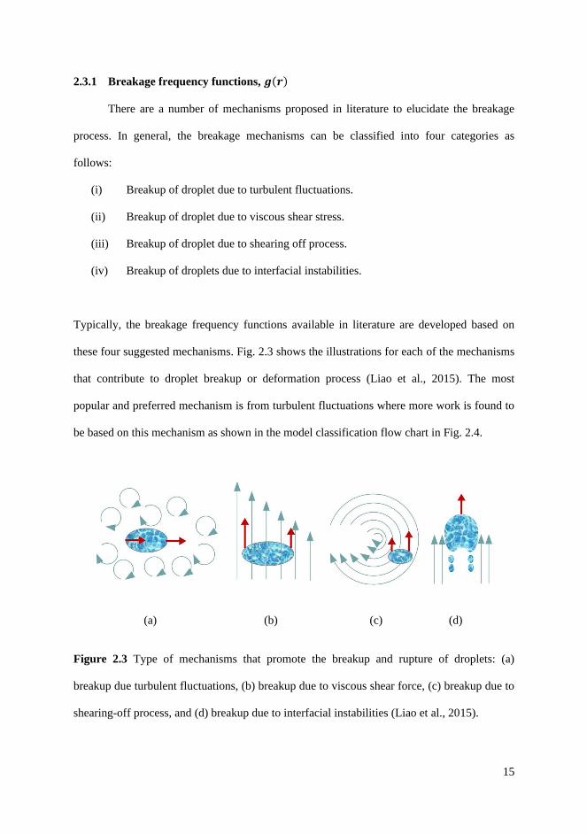
2.3.1 Breakage frequency functions, 𝒈(𝒓)
There are a number of mechanisms proposed in literature to elucidate the breakage
process. In general, the breakage mechanisms can be classified into four categories as
follows:
(i) Breakup of droplet due to turbulent fluctuations.
(ii) Breakup of droplet due to viscous shear stress.
(iii) Breakup of droplet due to shearing off process.
(iv) Breakup of droplets due to interfacial instabilities.
Typically, the breakage frequency functions available in literature are developed based on
these four suggested mechanisms. Fig. 2.3 shows the illustrations for each of the mechanisms
that contribute to droplet breakup or deformation process (Liao et al., 2015). The most
popular and preferred mechanism is from turbulent fluctuations where more work is found to
be based on this mechanism as shown in the model classification flow chart in Fig. 2.4.
(a) (b) (c) (d)
Figure 2.3 Type of mechanisms that promote the breakup and rupture of droplets: (a)
breakup due turbulent fluctuations, (b) breakup due to viscous shear force, (c) breakup due to
shearing-off process, and (d) breakup due to interfacial instabilities (Liao et al., 2015).

16
2.3.1.1 Breakup of droplets due to turbulent fluctuations
In this type of mechanism, the breakup of droplet is assumed to occur when there is an
imbalance between the dynamic forces (turbulent pressure fluctuations) and surface stresses
(surface energy) of the droplets. Based on this assumption, several criteria have been
proposed in the literature as follows:
• Turbulent kinetic energy being greater than surface energy
• Velocity fluctuation across the surface of the droplet
• Turbulent kinetic energy from fluctuating eddies being greater than surface energy
• Inertial force of the fluctuating eddies
The details of these criteria have been discussed in depth by Liao and Lucas, (2009), Abidin
et al., (2015), Solsvik et al., (2013) and Solsvik et al., (2014). Nevertheless, the pioneer of the
breakup model based on the criteria of turbulent kinetic energy being greater than surface
energy was proposed by Coulaloglou and Tavlarides (1977) and the model has been widely
used in literature. The criteria postulated that when the turbulent kinetic energy supplied from
turbulent eddies is large enough to overcome the critical value owned by each individual
droplet (the critical value in this context refers to the surface energy of the droplet). Hence,
the chaotic changes in velocity manifest the turbulent fluctuations and eventually promote the
particle-eddy collisions along the surface of the droplet. The continuous process of turbulent
fluctuations caused the droplet surface to become unstable. At higher oscillations, the process
leads to elongation and rupture of droplet into two or more daughter droplets. Hence, from
the assumptions discussed above, Coulaloglou and Tavlarides (1977) formulated the drop
breakage function as follows:
𝑔(𝑟) = (1
𝑏𝑟𝑒𝑎𝑘𝑎𝑔𝑒 𝑡𝑖𝑚𝑒) (
𝑓𝑟𝑎𝑐𝑡𝑖𝑜𝑛 𝑜𝑓𝑑𝑟𝑜𝑝𝑠 𝑏𝑟𝑒𝑎𝑘𝑖𝑛𝑔
) ≈1
𝑡𝑏𝑒𝑥𝑝 (−
𝐸𝜎
𝐸𝑘) (2.4)
17
Where, 𝑡𝑏 denotes the breakage time, 𝐸𝜎 and 𝐸𝑘 are the drop surface energy and kinetic
energy respectively. However, Lasheras et al., (2002) disagreed in general with the breakage
efficiency (the exponential term as shown in Table 2.1) proposed by Coulaloglou and
Tavlarides (1977) as they suggested that the breakup should be dependent more on
continuous phase density, 𝜌𝑐. Vankova et al., (2007) has extended the model by Coulaloglou
and Tavlarides (1977) and proposed drop breakage characterized by drop Reynolds number
(𝑅𝑒𝑑) that accounts for both continuous phase density, 𝜌𝑐 and dispersed phase density, 𝜌𝑑.
2.3.1.2 Breakup of droplets due to viscous shear stress
In this mechanism, the breakup of bubbles is assumed to occur when there is an
imbalance of forces between the external viscous stresses from the continuous fluid and
surface stresses of the droplets in the air-water mixture. In this respect, the viscous shear
stress from continuous fluid induced by the velocity gradient across the interface of the
droplet ultimately leads to droplet deformation. However, the deformation of the droplet is
based on the force balance characterized by the Capillary number, 𝐶𝑎. If 𝐶𝑎 is large enough
and above the critical value, the interfacial forces can no longer hold the particle intact and
eventually break the droplet into two or more daughter droplets.
2.3.1.3 Breakup of droplets due to shearing off process
In this mechanism, the breakage (erosive breakage) is assumed to occur when the
small bubbles are sheared off from the larger bubbles (Liao and Lucas, 2009). This process is
characterized by the imbalance of forces between the viscous shear force and surface tension
at skirts of the cap/slug bubble. For instance, in the case of viscous gas-liquid in turbulent
flows, the high relative velocity induces the bubble skirts to become unstable and
disintegrates them from larger droplets. This leads to generation of large number of small

18
droplets at the rim (i.e., boundary). The velocity difference around the interface of the particle
is the major contribution of this process (Fu and Isshi, 2002). Nevertheless, this mechanism is
the major concern only in case of air-water mixtures (gas-liquid flows) and was found to be
limited in the literature compared to turbulent fluctuations and viscous shear stress (Yeoh et
al., 2014).
2.3.1.4 Breakup of droplets due to interfacial instabilities
In this mechanism, the breakage is assumed to occur without the presence of net flow where
continuous fluid characteristics are insignificant. According to Liao and Lucas (2009) and
Solsvik et al., (2013 and 2014), breakage can still take place in a motionless liquid for
instance, the rise and fall of bubbles in continuous gas or immiscible liquids due to the
interfacial instabilities. This can be expressed in Rayleigh-Taylor instability wherein the low-
density fluid travels rapidly into a high-density fluid. In the case of density ratio approaching
unity, the breakage process is taking the Kelvin-Helmholtz instability.
Several models of breakage frequency functions 𝑔(𝑑) are derived from four different
criteria or mechanisms (see section 2.3.1.1) for droplets break process. For instance,
Coulaloglou and Tavlarides (1977) proposed a model for breakage frequency function mainly
on turbulent fluctuations. They assumed breakage rate to be a product of the fraction of
breaking drops and the reciprocal time needed for the drop breakup to occur as a result of
collision with turbulent eddy. They further added the factor of (1 + 𝜙) to account for the
damping effects on the local turbulent intensities at high hold up fractions. Chen et al. (1998)
introduced a mechanistic model for breakage rate function that accounts for interfacial
tension and viscosity. They also employed the effect of turbulent intensities at high holdup
fraction as suggested earlier by Coulaloglou and Tavlarides (1977). Rather simplistic, Cristini
et al., (2003) introduced a direct proportionality model or linear dependence based on sub-

19
Kolmogorov drops in terms of drop volume(𝑣), 𝑔(𝑣) ≈ 𝑘𝑣. Some of the breakage frequency
models in the literature are described in the Table 2.1. Majority of the proposed breakage
models are found to neglect the correction factor for dampening of turbulent intensities at
high dispersed phase fraction (1 + 𝜙) as suggested by Coulaloglou and Tavlarides (1977).
Figure 2.4 Mechanisms for breakage frequency

20
Ta
ble
2.1
Bre
akag
e fr
equen
cy f
unct
ion
s, 𝑔
(𝑟)
Au
thors
B
rea
ka
ge
freq
uen
cy (
rate
) fu
nct
ion
s, 𝒈
(𝒓)
Ass
essm
ents
of
the
mo
del
Cou
lalo
glo
u a
nd
Tav
lari
des
, (1
97
7)
𝑔( 𝑟
) =
𝑘𝑔
1
13
⁄
𝑟2
3⁄
( 1+
𝜙)ex
p[−
𝑘𝑔
2
𝜎( 1
+𝜙)2
𝜌𝑑
23
⁄𝑟
53
⁄]
Pre
dic
ts m
axim
um
dro
p b
reak
age
freq
uen
cy a
s th
e d
rop d
iam
eter
in
crea
ses.
Dev
elop
ed b
ased
on m
echan
ism
of
turb
ule
nt
flu
ctuat
ion
s an
d d
ampin
g
effe
ct (1
+𝜙)
for
a li
qu
id-l
iquid
sy
stem
wit
h h
igh d
isper
sed f
ract
ion
. T
he
exper
imen
tal
dat
a ar
e co
rrel
ated
sati
sfac
tori
ly w
ith
the
add
itio
n o
f
dam
pin
g f
acto
r in
the
bre
akag
e m
od
el.
Ho
wev
er, fo
r g
as-l
iquid
sy
stem
, th
is
bre
akag
e m
od
el p
redic
ts b
reak
up r
ate
low
er t
han
exp
erim
enta
l re
sult
s (P
rin
ce
and B
lan
ch 1
990).
This
is
due
to t
he
fact
that
, in
gas
-liq
uid
mix
ture
, th
e den
sity
is
low
er t
han
th
e den
sity
of
liq
uid
-liq
uid
dis
per
sio
ns.
Hen
ce, d
ensi
ty (𝜌
𝑑)
in t
he
bre
akag
e m
od
el s
hould
be
repla
ced b
y
den
sity
of
conti
nuo
us
phas
e, 𝜌
𝑐
Chen
et
al., (
199
8)
𝑔( 𝑟
)=
𝑘𝑔
1ex
p[−
𝑘𝑔
2𝜎( 1
+𝜙)2
𝜌𝑑𝑟
53
⁄2
3⁄
− 𝑘
𝑔3𝜇
𝑑( 1
+𝜙
)
𝜌𝑑𝑟
43
⁄1
3⁄
]
Mec
han
isti
c m
od
el w
hic
h i
nco
rpora
tes
inte
rfac
ial
tensi
on
, d
isp
erse
d d
ensi
ty a
nd
vis
cosi
ty. T
he
mo
del
is
a fu
nct
ion
of
loca
l
ener
gy p
er u
nit
mas
s. T
his
model
consi
der
s th
e vis
cou
s ef
fect
and
surf
ace
ener
gy i
n b
reak
up
fre
quen
cy o
f dro
ple
ts.

21
In t
his
pre
mis
e, a
flu
id w
ith
hig
h v
isco
sity
wil
l be
subje
cted
to d
eform
atio
n a
nd
stre
tch a
s in
tern
al v
isco
us
forc
e o
f th
e
dro
ple
t in
crea
ses
wh
ich
res
ult
s in
th
in
liq
uid
form
atio
n u
nti
l it
rea
ches
a c
riti
cal
thic
knes
s bef
ore
bre
akin
g/s
pli
ttin
g a
nd
pro
duci
ng m
ore
sm
alle
r d
rople
ts
(Ander
sso
n a
nd A
nd
erss
on, 2
006
). T
he
bre
akag
e ti
me
is a
ssum
ed t
o b
e co
nst
ant
(1𝑡 𝐵
=𝑘
𝑔1
⁄).
Alo
pae
us
et a
l.,
(20
02
) 𝑔( 𝑟
)=
𝑘𝑔
11
3⁄
ercf
(√
𝑘𝑔
2𝜎( 1
+𝜙)2
𝜌𝑐𝑟
53
⁄2
3⁄
+ 𝑘
𝑔3𝜇
𝑑( 1
+𝜙)
√𝜌
𝑐𝜌
𝑑𝑟
43
⁄1
3⁄
)
Acc
oun
ts f
or
dam
pin
g e
ffec
t at
hig
h
ph
ase
frac
tion
(1
+𝜙
) as
sug
ges
ted
by
Coula
log
lou
and T
avla
rides
, (1
977).
The
model
is
dev
elop
ed b
ased
on t
he
conce
pt
of
vel
oci
ty f
luct
uat
ion
theo
ry.
Th
e m
odel
is t
he
mod
ific
atio
n f
rom
th
e w
ork
of
Nar
sim
han
et
al.
(19
79
). T
hey
hav
e ad
ded
the
dro
p b
reak
age
mo
del
by a
ccou
nti
ng
the
dep
enden
cy o
n d
issi
pat
ion
rat
e an
d
vis
cous
forc
e w
hic
h h
as b
een
neg
lect
ed i
n
most
pre
vio
us
work
(L
iao
an
d L
uca
s,
20
09).
Th
e ef
fect
of
the
dro
p b
reak
up w
ill
dep
end
on t
he
mag
nit
ude
of
the
surf
ace
ten
sion
an
d d
isper
sed
ph
ase
vis
cosi
ty a
s
wel
l as
th
e fi
ttin
g p
aram
eter
s, 𝑘
𝑔1, 𝑘
𝑔2
and 𝑘
𝑔3.

22
Lu
o a
nd S
ven
dse
n,
(19
96)
𝑔( 𝑟
)
=𝑘( 1
−𝜙
)( 2
𝑟2)1
3⁄
∫( 1
+𝜉)2
𝜉11
3⁄
1
𝜉𝑚
𝑖𝑛
exp
( −12𝑐 𝑓
𝜎
𝛽𝜌
𝑐2
3⁄
𝑟5
3⁄
𝜉11
3⁄
)𝑑𝜉
Wh
ere,
𝑘=
15𝜋
13
⁄
8×
22
3⁄
𝛤(1
/3)𝛽
12
⁄
Th
e m
odel
is
der
ived
bas
ed o
n e
xte
nsi
on
of
the
clas
sica
l k
inet
ic t
heo
ry o
f g
ases
.
Th
e m
odel
ass
um
es t
hat
the
turb
ule
nce
consi
sts
of
an a
rray
of
dis
cret
e ed
die
s.
Th
e m
odel
does
not
pre
dic
t a
max
imum
bre
akag
e fr
equen
cy d
ue
to n
o l
imit
in t
he
low
er b
reak
up s
ize
or
refe
rence
on t
he
amo
unt
of
bre
akup.
Th
e m
odel
do
es n
ot
incl
ud
e an
y a
dju
stab
le p
aram
eter
an
d
dep
end
s st
rongly
on t
he
choic
e of
inte
gra
tion
lim
it w
hic
h i
s co
mm
on i
n t
he
wo
rk o
f P
rince
and B
lanch
, (1
99
0)
and
Tso
uri
s an
d T
avla
rid
es, (1
99
4).
Th
e
det
erm
inat
ion o
f lo
wer
an
d u
pper
in
tegra
l
lim
its
involv
es i
nd
irec
tly
tw
o u
nk
now
ns
(Lia
o a
nd L
uca
s, 2
009)
and
th
e m
odel
is
hig
hly
dep
enden
t up
on d
iscr
etiz
atio
n o
f
bu
bble
siz
e, a
nd
has
nei
ther
lim
it f
or
the
low
er b
reak
up s
ize
no
r an
y r
efer
ence
on
the
amoun
t o
f bre
aku
p (
Wan
g e
t al
.,
20
03;
Hag
esae
ther
et
al., 1
999).
The
model
has
rec
eived
num
erou
s
dis
agre
emen
ts (
Saj
jad
i et
al.
, 2
013
).
Chat
zi a
nd L
ee,
(19
87);
Ch
atzi
et
al.,
(19
89)
𝑔( 𝑟
)=
𝑘𝑔
1𝑟
−2
3⁄
13
⁄(
2 √𝜋).𝛤
(3 2
,𝑘
𝑔2𝜎
𝜌𝑑
23
⁄𝑟
53
⁄)
Dev
elop
ed f
rom
turb
ule
nt
flu
ctuat
ion
s
theo
ry.
The
dif
fere
nce
bet
wee
n t
he
oth
er
model
s is
the
pro
bab
ilit
y d
ensi
ty f
unct
ion
of
the
turb
ule
nt
kin
etic
ener
gy i
s
expre
ssed
by M
axw
ell’
s la
w. T
he

23
dau
ghte
r dro
ple
t si
ze d
istr
ibuti
on i
s
esti
mat
ed f
rom
no
rmal
fu
nct
ion m
od
el.
Ho
wev
er, th
e m
odel
rec
eiv
ed c
riti
cs f
rom
Lu
o a
nd S
ven
dse
n, (1
99
6)
since
th
e
Max
wel
l’s
law
is
app
rop
riat
e fo
r fr
ee g
as
mole
cula
r m
oti
on,
thus,
may
not
suit
able
for
imag
inar
y e
dd
ies.
T
he
model
does
not
acco
unt
the
dam
pin
g e
ffec
t, (1
+𝜙)
as
sugges
ted b
y C
ou
lalo
glo
u a
nd T
avla
rid
es,
(19
77)
and n
ot
suit
able
for
gas
-liq
uid
syst
em (
Saj
jadi
et a
l.,
201
3)
Mar
tínez
-Baz
án e
t al
.,
(19
99)
𝑔( 𝑟
)=
𝑘𝑔
1
√𝑘
𝑔2(
𝑟)2
3⁄
−6
𝜎 𝜌𝑐𝑟
𝑟
Th
e m
odel
is
bas
ed o
n p
ure
ly k
inem
atic
idea
s fo
r fu
lly
dev
elop
ed t
urb
ule
nt
flo
ws.
Th
e m
odel
ass
um
ed t
hat
surf
ace
of
a
dro
ple
t m
ust
be
def
orm
ed f
or
a dro
ple
t to
bre
ak.
In t
his
pre
mis
e, s
uff
icie
nt
ener
gy
must
be
avai
lable
by t
he
turb
ule
nt
stre
sses
in t
he
surr
oun
din
g c
onti
nuo
us
fluid
. T
his
model
is
sim
ilar
to o
ther
model
s w
her
ein
,
the
dro
ple
t w
ill
bre
ak i
f th
e tu
rbu
lent
kin
etic
en
erg
y i
n c
onti
nu
ous
phas
e is
gre
ater
than
a c
riti
cal
val
ue.
The
dif
fere
nce
s b
etw
een
oth
er m
odel
s ar
e th
at
this
mod
el n
egle
ct t
he
pro
bab
ilit
y t
heo
ry
for
the
dis
trib
uti
on d
ensi
ty o
f kin
etic
ener
gy o
r v
eloci
ty f
luct
uat
ions
as w
ell
as
dis
card
the
dam
pin
g e
ffec
t at
hig
h
dis
per
sed
fra
ctio
n (1
+𝜙
).

24
Leh
r et
al.
, (2
00
2)
𝑔( 𝑟
)=
25
3⁄ 2
𝑟5
3⁄
19
15
⁄𝜌
𝑐75
⁄
𝜎7
5⁄
𝑒𝑥𝑝
(−
√2𝜎
95
⁄
8𝑟
3𝜌
𝑐95
⁄6
5⁄
)
Th
e m
odel
dev
elo
ped
bas
ed o
n f
orc
e
bal
ance
bet
wee
n t
he
iner
tial
forc
e o
f th
e
eddy
an
d t
he
inte
rfac
ial
forc
e of
the
dau
ghte
r dro
ps.
Th
e m
od
el i
s th
e
impro
ved
ver
sion
fro
m L
ehr
and
Mew
es,
(19
99).
Th
is m
od
el p
rop
ose
d t
he
bre
akup
pro
bab
ilit
y b
ased
on t
he
con
cep
t th
at
kin
etic
en
erg
y o
f th
e ed
dy m
ust
ex
ceed
s
the
crit
ical
en
erg
y.
This
has
to b
e
ob
tain
ed f
rom
forc
e b
alan
ce e
qu
atio
n.
On
e u
niq
ue
feat
ure
of
this
model
is
that
,
the
pro
bab
ilit
y o
f th
e bub
ble
to b
reak
in
to
two d
aug
hte
r dro
ple
ts a
nd
its
com
pli
men
tary
par
t is
co
mpute
d b
y
dif
fere
nti
atin
g t
he
tota
l b
reak
up
pro
bab
ilit
y o
f th
e par
ent
dro
ple
t. T
he
model
dis
counte
d t
he
angle
un
der
whic
h
the
eddy h
its
the
dro
ple
ts (
Lia
o a
nd
Lu
cas,
20
10)
and t
he
dam
pin
g e
ffec
t at
hig
h v
olu
me
frac
tions
(1+
𝜙).
Van
ko
va
et a
l.,
(200
7)
𝑔( 𝑟
)=
𝑘𝑔
1
13
⁄
𝑟2
3⁄
√𝜌
𝑐
𝜌𝑑𝑒𝑥
𝑝[−
𝑘𝑔
2
𝜎
𝜌𝑑 𝑟
53
⁄2
3⁄
]
Th
e m
odel
is
expre
ssed
in t
erm
s of
turb
ule
nt
flu
ctuat
ions
that
aff
ects
the
inte
rnal
mo
tion
of
dro
p i
n l
iquid
. T
he
model
ass
um
ed t
hat
th
e ed
die
s w
ith s
ize
com
par
able
to t
he
dro
p d
imet
er, 𝑑
, a
re
mo
st e
ffic
ien
t in
cau
sing
dro
p b
reak
age,
bec
ause
th
e sm
alle
r ed
die
s hav
e m
uch
low
er e
ner
gy
and
the
larg
er e
ddie
s ar
e

25
bel
ieved
to h
ave
dra
g t
he
dro
ple
t in
stea
d
of
def
orm
ing i
t. T
he
mo
del
als
o u
tili
zes
the
rela
tionsh
ip b
etw
een
th
e R
eyno
lds
nu
mb
er i
n t
he
dro
ps
wit
h t
he
vel
oci
ty o
f
the
liq
uid
insi
de
the
dro
ps
to e
stim
ate
the
def
orm
atio
n t
ime.
The
mo
del
dep
ends
on
the
rati
o o
f th
e den
sity
bet
wee
n
conti
nuo
us
and d
isper
sed
of
less
vis
cous
flu
ids
and d
isco
unts
th
e d
ampin
g f
acto
r of
( 1+
𝜙)
at h
igh d
isper
sed f
ract
ion
. T
he
mai
n p
aram
eter
s co
ntr
oll
ing
rat
e o
f
bre
akag
e o
f th
is m
odel
are
en
ergy
dis
sipat
ion
rat
e,
and
in
terf
acia
l te
nsi
on
,
𝜎.

26
2.3.2 Daughter size distribution (breakage probability), 𝛃(𝒓, 𝒓′)
In order to have a complete description of the breakage sub-process, it is necessary to
consider the daughter size distribution in terms of the number of drops formed and their
distribution. The model has to be developed separately from the breakage frequency. The
main goal of this function is to determine the probability of a certain size of droplets formed
as a result of bigger droplets being ruptured. The daughter size distribution is composed of a
probability density function and the number of drops formed after the breakage process. Most
of the modelling works describe breakage as a series of binary breakage processes (Raikar,
2010). There are limited numbers of experimental and modelling studies for daughter size
distribution with multiple and/or unequal size daughter droplets or combination of equal and
unequal size daughter droplets to account for breakage event (Abidin et al., 2015). In general,
the average number of daughter droplets formed depends on the forces applied, diameter, and
the interfacial tension of the parent droplet (Hsia and Tavlarides, 1980). Based on these
requirements, the daughter size distribution can be classified into three categories namely,
empirical, statistical, and phenomenological.
2.3.2.1 Empirical model
Empirical model is formulated based on observation and experiment. Hence, it is considered
as case specific (i.e., for a specific application and system). Thus, the model is normally not
considered or preferred for the droplet size distribution. According to Solsvik et al., (2013),
the empirical model limits the range of applications and is incapable of extrapolating outside
of the operational conditions for which the model parameters were determined. In this
respect, generalized model is more applicable where the number and size of droplets formed
from a breakage event can be decently described regardless of the conditions (i.e., liquid-
liquid or gas-liquid, stir tank or pipe flow). Hesketh et al., (1991) developed an empirical

27
model to determine the daughter size distribution in their study of bubble breakage in air-
water pipeline flow.
2.3.2.2 Statistical model
In statistical approach, the size of the daughter droplets is usually described by the random
variable and its probability distribution function proposed satisfies a simple expression. The
common expressions used are as follows:
• Normal or Gaussian distribution
• Beta (β) distribution
• Uniform distribution
The normal density function was first introduced by Valentas et al., (1966) which later
became widely used for investigations such as Coulaloglou and Tavlarides (1977), Chatzi et
al., (1989), Lasheras (2002), and Raikar (2010). On the other hand, beta (β) distribution has
been proposed by Hsia and Tavlarides in 1980 by modifying their earlier work. One of the
advantages of beta (β) distribution is preventing zero probability for the evolution of equal-
sized droplets as compared to other models (Azizi and Taweel, 2011). Nevertheless,
Narsimhan et al., (1979) and Randolph, (1969) suggested that a random (uniform)
distribution for binary breakage could be used to describe the droplets formed from the
breakage event in agitated liquid-liquid dispersions. There has been disagreement reported
from this assumption by Sajjadi et al., (2013) and Liao and Lucas, (2009) because nature does
not split liquid volumes at random (Villermaux, 2007).
2.3.2.3 Phenomenological model
In the phenomenological model, the underlying concept is to relate empirical observations of
important phenomena that corresponds to fundamental theory but is not directly derived from

28
the theory. In this respect, the underlying theory of such phenomena is not fully understood
and may not yet have been discovered (Liao and Lucas, 2009) or the mathematics to describe
such phenomena are too complex (Solsvik et al., 2013). From the shape of the daughter size
distribution, the proposed phenomenological models are comprised of functions that are
generally classified as U-shaped, Bell-shaped, and M-shaped. As reported by Abidin et al.,
(2015), the most widely used phenomenological model for the daughter size distribution is
from the bimodal U-shaped function developed by Tsouris and Tavlarides, (1994). This is a
model with highest probability density when one of the daughters has a minimum diameter
(parent droplet unlikely to break) and lower probability density for two daughter droplets of
same size. The model was developed based on the energy requirements for the daughter
drops formation. In comparison to beta (β) distribution function, this model by Tsouris and
Tavlarides, (1994) yielded minimum probability at equal size breakage while, beta (β)
function produced maximum probability at equal size breakage which is the opposite of this
model. However, the advantage of beta distribution model is that it predicts zero probability
for daughter droplets with size equal to parent droplet and for droplets infinitely small
(Abidin et al., 2015). In addition, the beta (β) distribution function is also capable to account
for the total volume of droplets within the lower and upper limits of droplet size (Abidin et
al., 2015). Luo and Svendsen, (1996) also proposed the U-shaped model for the daughter size
distribution for drop breakage. The model has similar criteria with Tsouris and Tavlarides,
(1994) where the probability is minimum at equal size breakage at maximum the volume
fraction approaches zero or unity. Furthermore, the model has a non-zero minimum and
mainly relies on the size of the parent droplet (Liao and Lucas, 2009). All the models
discussed above for daughter size distribution are presented in the diagram as shown in Fig.
2.5 below.
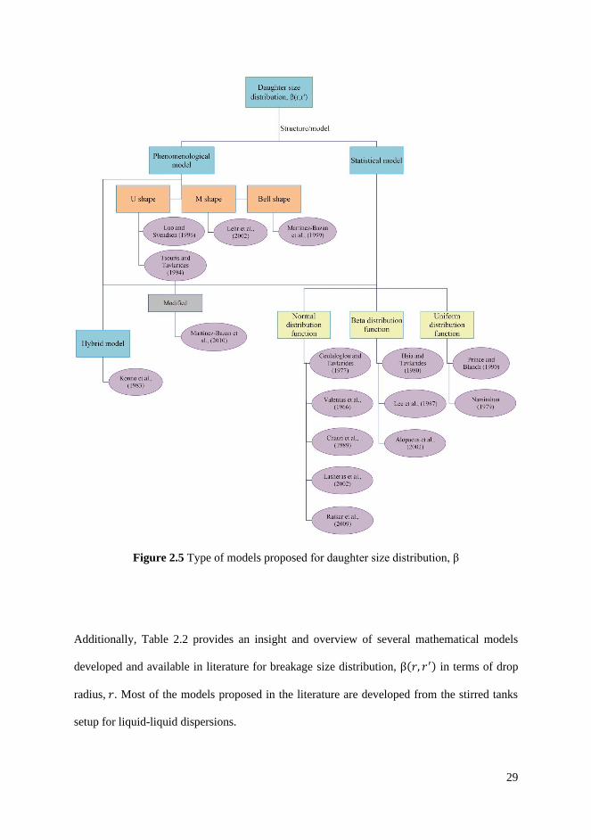
29
Figure 2.5 Type of models proposed for daughter size distribution, β
Additionally, Table 2.2 provides an insight and overview of several mathematical models
developed and available in literature for breakage size distribution, β(𝑟, 𝑟′) in terms of drop
radius, 𝑟. Most of the models proposed in the literature are developed from the stirred tanks
setup for liquid-liquid dispersions.
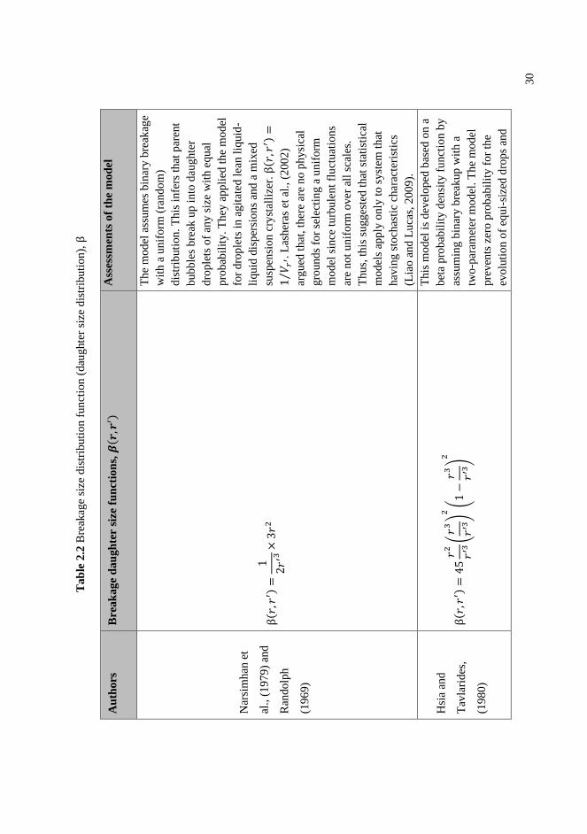
30
Ta
ble
2.2
Bre
akag
e si
ze d
istr
ibu
tio
n f
un
ctio
n (
dau
gh
ter
size
dis
trib
uti
on),
β
Au
tho
rs
Bre
ak
age
da
ugh
ter
size
fu
nct
ion
s, 𝜷
( 𝒓,𝒓
′ )
Ass
essm
ents
of
the
mod
el
Nar
sim
han
et
al.,
(1
979
) an
d
Ran
do
lph
(196
9)
β( 𝑟
,𝑟′ )
=1
2𝑟
′3×
3𝑟
2
The
mo
del
ass
um
es b
inar
y b
reak
age
wit
h a
un
iform
(ra
ndo
m)
dis
trib
uti
on
. T
his
infe
rs t
hat
par
ent
bub
ble
s bre
ak u
p i
nto
dau
gh
ter
dro
ple
ts o
f an
y s
ize
wit
h e
qu
al
pro
bab
ilit
y.
They
appli
ed t
he
mo
del
for
dro
ple
ts i
n a
git
ated
lea
n l
iquid
-
liqu
id d
isper
sio
ns
and a
mix
ed
susp
ensi
on c
ryst
alli
zer.
β( 𝑟
,𝑟′ )
=
1𝑉 𝑟
′⁄
. L
ash
eras
et
al., (
200
2)
arg
ued
that
, th
ere
are
no
ph
ysi
cal
gro
und
s fo
r se
lect
ing
a u
nif
orm
mo
del
sin
ce t
urb
ule
nt
flu
ctuat
ion
s
are
not
unif
orm
over
all
sca
les.
Thu
s, t
his
su
gg
este
d t
hat
sta
tist
ical
mo
del
s ap
ply
only
to s
yst
em t
hat
hav
ing s
toch
asti
c ch
arac
teri
stic
s
(Lia
o a
nd
Lu
cas,
2009
).
Hsi
a an
d
Tav
lari
des
,
(198
0)
β( 𝑟
,𝑟′ )
=45
𝑟2
𝑟′3
(𝑟
3
𝑟′3)
2
(1
−𝑟
3
𝑟′3)
2
This
mo
del
is
dev
eloped
bas
ed o
n a
bet
a pro
bab
ilit
y d
ensi
ty f
un
ctio
n b
y
assu
min
g b
inar
y b
reak
up
wit
h a
two
-par
amet
er m
od
el. T
he
mod
el
pre
ven
ts z
ero
pro
bab
ilit
y f
or
the
evolu
tion o
f eq
ui-
size
d d
rops
and
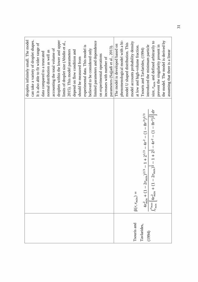
31
dro
ple
ts i
nfi
nit
ely s
mal
l. T
he
mod
el
can t
ake
a var
iety
of
dro
ple
t sh
apes
.
It i
s al
so a
ble
to f
it w
ider
ran
ge
of
dat
a co
mp
ared
to a
tru
nca
ted
norm
al d
istr
ibu
tion
as
wel
l as
acco
unti
ng t
he
tota
l vo
lum
e o
f
dro
ple
ts w
ithin
th
e lo
wer
an
d u
pper
lim
its
of
dro
ple
t si
ze (
Abid
in e
t al
.,
201
5).
This
mo
del
par
amet
ers
dep
end o
n f
low
cond
itio
n a
nd
shou
ld b
e m
easu
red f
rom
exper
imen
tal
dat
a. T
his
model
is
bel
ieved
to
be
con
sid
ered
only
lim
ited
par
amet
ers
and d
epen
den
ce
on e
xp
erim
enta
l op
erat
ions
incr
ease
s w
ith n
um
ber
of
par
amet
ers
(Saj
jad
i et
al.
, 201
3).
Tso
uri
s an
d
Tav
lari
des
,
(199
4)
β( 𝑟
,𝑟𝑚
𝑖𝑛)=
4𝑟 𝑚
𝑖𝑛2
+( 1
−2𝑟 𝑚
𝑖𝑛)2
3⁄
−1
+2
13
⁄−
4𝑟
2−
( 1−
8𝑟
3)2
3⁄
∫[4
𝑟 𝑚𝑖𝑛
2+
( 1−
2𝑟 𝑚
𝑖𝑛)1 3
−1
+2
1 3−
4𝑟
2−
( 1−
8𝑟
3)2 3
]𝑟 𝑚
𝑎𝑥
𝑟𝑚
𝑖𝑛𝑑𝑟
The
mo
del
is
dev
eloped
bas
ed o
n
phen
om
eno
logic
al m
odel
wit
h a
bi-
mo
del
U s
hap
ed d
istr
ibu
tion.
This
mo
del
acc
ounts
pro
bab
ilit
y d
ensi
ty
at l
ow
and
hig
h-v
olu
me
frac
tion.
Tso
uri
s an
d T
avla
rid
es, (1
994
)
intr
oduce
d t
he
min
imu
m p
arti
cle
size
, 𝑟 𝑚
𝑖𝑛 a
nd
def
ined
arb
itra
rily
to
pre
ven
t th
e si
ngu
lari
ty p
rese
nt
in
the
mod
el.
The
mod
el i
s der
ived
by
assu
min
g t
hat
ther
e is
a l
inea
r

32
rela
tion b
etw
een e
ner
gy
requir
emen
ts f
or
the
form
atio
n o
f
dau
gh
ter
dro
ple
ts a
nd d
aughte
r si
ze
dis
trib
uti
on
funct
ion
, an
d m
inim
al
ener
gy i
s re
qu
ired
fo
r dro
p b
reak
age
(Saj
jadi
et a
l.,
201
3).
This
mo
del
also
av
oid
s eq
ual
bre
akag
e an
d
pre
dic
ts t
he
min
imum
pro
bab
ilit
y
for
dau
gh
ter
dro
ple
ts w
ith e
qual
size
bre
akag
e an
d h
ighes
t
pro
bab
ilit
y f
or
ver
y l
arge
dro
ple
ts.
Ind
epen
den
t o
f par
ent
size
and
flo
w
condit
ions,
how
ever
the
bre
akag
e
ker
nel
does
not
sati
sfy t
he
sym
met
ry c
ond
itio
n a
nd
pre
serv
e
the
volu
me
(So
lsvik
et
al., 2
013
).
Mar
tínez
-Baz
án
et a
l., (2
01
0)
β( 𝑟
,𝑟𝑚
𝑖𝑛)=
[(4𝑟 𝑚
𝑖𝑛2
+( 1
−8𝑟 𝑚
𝑖𝑛3
)2 3−
1)
+2
1 3−
4𝑟
2−
( 1−
8𝑟
3)2 3
]4𝑟
2
∫[(
4𝑟 𝑚
𝑖𝑛2
+( 1
−8𝑟 𝑚
𝑖𝑛3
)2 3−
1)
+2
1 3−
4𝑟
2−
( 1−
8𝑟
3)2 3
]𝑟 𝑚
𝑎𝑥
𝑟𝑚
𝑖𝑛4𝑟
2𝑑𝑟
The
mo
del
is
bas
ed f
rom
phen
om
eno
logic
al c
ondit
ion t
hat
rela
tes
emp
iric
al o
bse
rvat
ion
s o
f
phen
om
enon t
o e
ach o
ther
.
Mar
tín
ez-B
azán
et
al.,
(2
01
0)
der
ived
th
e dau
ghte
r si
ze
dis
trib
uti
on
s as
a f
unct
ion o
f bel
l-
shap
e dis
trib
uti
on f
rom
str
ess
bal
ance
. H
ence
, fr
om
the
mod
el,
form
atio
n o
f d
aug
hte
r dro
ple
ts w
ith
equal
siz
e h
ave
the
hig
hes
t
pro
bab
ilit
y, w
hil
e o
ne
larg
e an
d o
ne
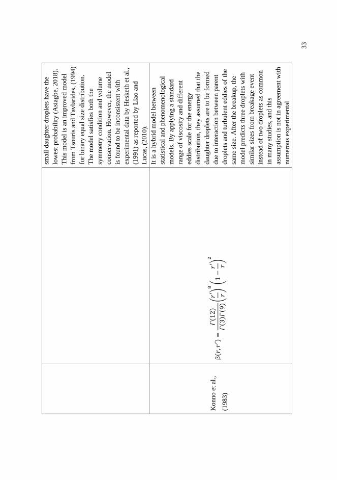
33
smal
l d
augh
ter
dro
ple
ts h
ave
the
low
est
pro
bab
ilit
y (
Asi
agb
e, 2
01
8).
This
mo
del
is
an i
mpro
ved
mod
el
fro
m T
sou
ris
and
Tav
lari
des
, (1
994)
for
bin
ary e
qu
al s
ize
dis
trib
uti
on
.
The
mo
del
sat
isfi
es b
oth
the
sym
met
ry c
ond
itio
n a
nd
vo
lum
e
conse
rvat
ion
. H
ow
ever
, th
e m
odel
is f
ound
to b
e in
consi
sten
t w
ith
exper
imen
tal
dat
a by H
esk
eth e
t al
.,
(199
1)
as r
epo
rted
by L
iao a
nd
Luca
s, (
201
0).
Kon
no e
t al
.,
(198
3)
β( 𝑟
,𝑟′ )
=𝛤( 1
2)
𝛤( 3
) 𝛤( 9
)(𝑟
′ 𝑟)
8
(1
−𝑟
′ 𝑟)
2
It i
s a
hyb
rid
model
bet
wee
n
stat
isti
cal
and
phen
om
enolo
gic
al
mo
del
s. B
y a
pply
ing a
sta
nd
ard
range
of
vis
cosi
ty a
nd
dif
fere
nt
eddie
s sc
ale
for
the
ener
gy
dis
trib
uti
on
, th
ey a
ssu
med
th
at t
he
dau
gh
ter
dro
ple
ts a
re t
o b
e fo
rmed
due
to i
nte
ract
ion b
etw
een p
aren
t
dro
ple
ts a
nd
tu
rbu
lent
eddie
s of
the
sam
e si
ze. A
fter
the
bre
akup,
the
mo
del
pre
dic
ts t
hre
e d
rop
lets
wit
h
sim
ilar
siz
es f
rom
bre
akag
e ev
ent
inst
ead
of
two
dro
ple
ts a
s co
mm
on
in m
any s
tud
ies,
and t
his
assu
mp
tion
is
no
t in
ag
reem
ent
wit
h
num
erou
s ex
per
imen
tal

34
inv
esti
gat
ion
s (i
.e., H
esk
eth e
t al
.,
199
1;
Ander
sson a
nd A
nd
erss
on,
200
6).
The
mo
del
als
o i
s no
t
volu
me
conse
rved
, h
ence
is
no
t
accu
rate
mod
elli
ng o
f li
quid
dis
per
sion
s (S
ols
vik
et
al., 2
013
).
Co
ula
log
lu a
nd
Tav
lari
des
,
(197
7)
β( 𝑟
,𝑟′ )
= 0
.3
𝑟′3
exp
[−4.5
( 16𝑟
3−
8𝑟
′3)2
( 2𝑟
′ )6
]
The
mo
del
is
dev
eloped
bas
ed o
n
stat
isti
cal
app
roac
h b
y a
ssum
ing
that
the
funct
ion i
s n
orm
ally
dis
trib
ute
d s
imil
ar t
o C
hat
zi e
t al
.,
(198
9)
and V
alen
tas
et a
l., (1
96
6).
The
mo
del
ass
um
es b
inar
y b
reak
age
and p
rovid
es m
axim
um
pro
bab
ilit
y
bre
akag
e fo
r eq
ual
siz
e d
aughte
r
dro
ple
ts.
They
als
o f
ixed
the
stan
dar
d d
evia
tio
n, 𝜎
𝑉 s
uch
that
>
99.6
% o
f th
e par
ticl
e fo
rmed
wer
e
wit
hin
the
vo
lum
e ra
nge
𝑉 𝑟∈
[ 0,𝑉
𝑟′]
wh
en 𝑐
=3
(L
iao a
nd
Luca
s, 2
00
9;
Sols
vik
et
al., 2
013).
Lee
et
al.,
(198
7)
β( 𝑟
,𝑟′ )
=𝛤( 𝑎
+𝑏)
𝛤( 𝑎
) 𝛤( 𝑏
)(𝑟
′ 𝑟)
𝑎−
1
(1
−𝑟
′ 𝑟)
𝑏−
1
The
mo
del
dev
eloped
is
bas
ed o
n
bet
a dis
trib
uti
on
for
bin
ary
bre
akag
e an
d a
lmost
sim
ilar
to t
he
dis
trib
uti
on
pro
po
sed
by K
onno
et
al., (
19
83).
The
auth
ors
em
phas
ized
that
the
mod
el i
s b
est
fitt
ed f
or
mu
lti-
bre
akag
e m
od
el (
Sols
vik
et
al., 2
013).
The
par
amet
ers 𝑎
an
d 𝑏

35
are
det
erm
ined
em
pir
ical
ly w
ith
exper
imen
tal
dat
a of
bub
ble
bre
akag
e ob
tain
ed f
rom
an a
irli
ft
colu
mn.
Acc
ord
ing t
o L
ee e
t al
.,
(198
7),
fo
r bin
ary b
reak
age
the
bes
t
val
ue
for 𝑎
an
d 𝑏
is
2.0
. H
ow
ever
,
the
model
is
fou
nd t
o a
pply
fo
r a
mu
lti-
bre
akag
e m
od
el i
n w
hic
h
num
ber
of
dau
gh
ter
par
ticl
es d
id
var
y w
ith t
he
moth
er p
arti
cle
size
(So
lsv
ik e
t al
., 2
013
).
Leh
r et
al.
,
(200
2)
β( 𝑟
,𝑟′ )
=
1
√𝜋
(𝑟′3 𝑟3)
.
exp
{−9 4
[(2
25
⁄𝜌
𝑐35
⁄2
5⁄
𝜎3
5⁄
)]}
{1+
𝑒𝑟𝑓
[3 2ln
(2
115
⁄𝜌
𝑐35
⁄2
5⁄
𝜎3
5⁄
)]}
This
mo
del
is
bas
ed o
n
phen
om
eno
logic
al m
odel
wit
h M
-
shap
ed d
istr
ibu
tion.
In t
his
model
,
the
dau
ghte
r dro
ple
t d
istr
ibuti
on i
s
dep
enden
t on t
he
par
ent
size
as
such
, th
e pro
bab
ilit
y o
f sm
all
and
larg
e d
aughte
r dro
ple
ts i
ncr
ease
s
sign
ific
antl
y w
ith t
he
par
ent
size
.
They
ass
um
ed t
hat
on
ly e
ddie
s th
at
are
big
ger
th
an t
he
smal
lest
dau
gh
ter
dro
ple
t ar
e ab
le t
o c
arry
the
dau
ghte
r d
rople
t aw
ay.
The
mo
del
dis
trib
uti
on c
han
ges
fro
m
mo
no
-mo
dal
to b
i-m
odal
wit
h t
he
incr
ease
of
the
par
ent
dro
ple
t si
ze.
They
rep
ort
ed t
hat
by i
ncr
easi
ng t
he
par
ent
dro
ple
t d
iam
eter
, th
e

36
pro
bab
ilit
y o
f pro
du
cing e
qual
dau
gh
ter
dro
ple
t si
ze d
ecre
ases
and
uneq
ual
bre
akag
e is
pre
ferr
ed.
Thu
s, i
t bec
om
es M
-sh
aped
for
big
ger
dro
ps
and f
inal
ly U
-sh
aped
for
ver
y b
ig m
oth
er d
rople
ts
(Saj
jadi
et a
l.,
20
13).
The
model
pre
dic
ts t
he
equ
al-s
ize
bre
akag
e is
mo
re l
ikel
y a
t sm
all
dro
ple
ts t
han
big
dro
ple
ts. H
ow
ever
, so
far
ther
e
is n
o e
xper
imen
tal
evid
ence
or
theo
reti
cal
sup
port
pre
sente
d (
Lia
o
and L
uca
s, 2
010
).
Hes
ket
h e
t al
.,
(199
1)
β( 𝑟
,𝑟′ )
=[
1
(𝑟 𝑟′)
3
+𝐵
+1
1−
(𝑟 𝑟′)
3
+𝐵
−2
𝐵+
1 2
]×
𝐴
2𝑟
′3𝑟
2
1 𝐴=
2[𝑙
𝑛( 1
+𝐶)−
𝑙𝑛( 𝐷
)−
1−
2(𝑟 𝑚
𝑖𝑛
𝑟′
)3
𝐵+
0.5
]
𝐶=
𝐵−
(𝑟 𝑚𝑖𝑛
𝑟′
)3
,𝐷
=𝐵
+(𝑟 𝑚
𝑖𝑛
𝑟′
)3
Hes
ket
h e
t al
., (
19
91
) dev
elop
ed t
he
mo
del
bas
ed o
n t
he
exp
erim
ent
per
form
ed o
n b
ubb
le b
reak
age
in
turb
ule
nt
pip
e fl
ow
. T
hey
com
par
ed
sever
al d
aug
hte
r si
ze d
istr
ibuti
on
funct
ions
whic
h i
ncl
ude,
bin
ary
equal
-volu
me
bre
akag
e, r
ando
m
bre
akag
e, 1
/𝑋-s
hap
ed b
reak
age,
and a
ttri
tio
n. T
he
attr
itio
n b
reak
age
is d
escr
ibed
as
a bre
akag
e in
wh
ich
a v
ery s
mal
l bu
bb
le a
nd a
bub
ble
of
nea
rly t
he
sam
e si
ze a
s th
e
bre
akin
g b
ubb
le i
s fo
rmed
. W
hil
e,
1/𝑋
-sh
aped
(as
dep
icte
d i
n t
his
Tab
le 2
.2)
is a
bre
akag
e fu
nct
ion

37
sim
ilar
to a
ttri
tion b
ut
allo
ws
bub
ble
s si
ze o
f an
y s
ize
less
than
, 𝑟
′
to b
e fo
rmed
. T
hey
foun
d t
hat
, th
e
rando
m b
reak
age
ov
erpre
dic
ted
th
e
dau
gh
ter
dro
ple
ts a
nd
att
riti
on
bre
akag
e ov
erpre
dic
ted
the
form
atio
n o
f sm
all
dau
gh
ter
dro
ple
ts. T
he
bes
t fi
t m
od
el w
ith t
he
exper
imen
tal
dat
a is
1/𝑋
-shap
ed
bre
akag
e. T
his
mod
el p
rodu
ces
hig
her
pro
bab
ilit
y f
or
un
equal
siz
e
dro
ple
ts t
han
equal
siz
e d
rople
ts.
How
ever
, th
e m
odel
par
amet
er
val
ues
wil
l var
y w
ith
dif
fere
nt
flow
condit
ions
and
wit
h i
nit
ial
dro
ple
t
size
(L
ash
eras
et
al.,
20
02).
Thus,
this
mo
del
has
no
ph
ysi
cal
just
ific
atio
n a
nd i
s co
nsi
der
ed a
s
empir
ical
mod
el b
ut
can
be
use
d f
or
com
par
iso
n w
ith
the
phen
om
eno
logic
al m
odel
(S
ols
vik
et a
l.,
2013
).
Val
enta
s et
al.
,
(196
6)
β( 𝑟
,�̅�)=
1
𝜎𝑑√2𝜋
𝑒𝑥𝑝
(−
2( 𝑟
−�̅�)
2
𝜎𝑑2
)
Bas
ed o
n n
orm
al (
Gau
ssia
n)
dis
trib
uti
on
. T
his
mod
el w
as f
irst
to
be
dev
elop
ed b
y V
alen
tas
et a
l.,
(196
6)
fro
m t
run
cate
d n
orm
al
pro
bab
ilit
y d
ensi
ty f
unct
ion.
The
mo
del
ass
um
es t
hat
the
dau
ghte
r
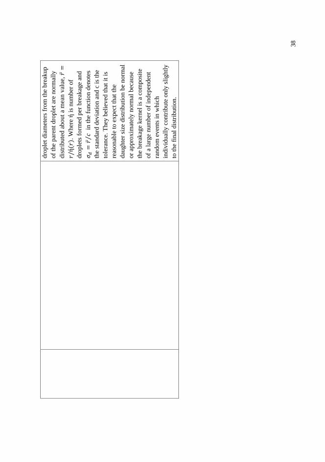
38
dro
ple
t dia
met
ers
fro
m t
he
bre
akup
of
the
par
ent
dro
ple
t ar
e norm
ally
dis
trib
ute
d a
bo
ut
a m
ean v
alue,
�̅�=
𝑟/ή(𝑟
). W
her
e ή
is
nu
mber
of
dro
ple
ts f
orm
ed p
er b
reak
age
and
𝜎𝑑
=�̅�
𝑐⁄
in
th
e fu
nct
ion d
eno
tes
the
stan
dar
d d
evia
tion a
nd c
is
the
tole
rance
. T
hey
bel
iev
ed t
hat
it
is
reas
onab
le t
o e
xpec
t th
at t
he
dau
gh
ter
size
dis
trib
uti
on
be
no
rmal
or
app
roxim
atel
y n
orm
al b
ecau
se
the
bre
akag
e ker
nel
is
a co
mposi
te
of
a la
rge
num
ber
of
ind
epen
den
t
rando
m e
ven
ts i
n w
hic
h
ind
ivid
ual
ly c
ontr
ibute
only
sli
ghtl
y
to t
he
final
dis
trib
uti
on.
39
2.4 Review of coalescence model
Apart from breakage process, coalescence is also responsible for the evolution of
droplets in liquid-liquid or gas-liquid flows. In general, coalescence is a process when two or
more droplets are merging to form a droplet. In this respect, the process is typically
associated with contact and collision between droplets. In turbulence, the coalescence process
is considered complex (Chesters, 1991) due to the interactions of droplets with surrounding
continuous liquid and alongside other droplets. The coalescence model is normally expressed
as the product of collision frequency, 𝜔𝐶 and coalescence efficiency functions, 𝜓𝐸 . There are
several models proposed in literature to calculate the collision frequency, 𝜔𝐶 and coalescence
efficiency functions, 𝜓𝐸 . Among the earliest models studied on coalescence are the ones by
von Smoluchowski, (1917) who investigated the aggregation of particles by Brownian motion
and Valentas and Amundson, (1966) that proposed mathematical descriptions for coalescence
based on a film drainage process. The most widely applied modeling approach for
coalescence is the film drainage model (Liao and Lucas, 2010). Film drainage is a process in
which when the droplets collide, they will trap a small film of liquid between them. As they
remain in contact, the liquid film separating the droplets slowly drains out to a critical
thickness and eventually ruptures due to film instabilities which lead to formation of a single
new droplet. In this section, a number of proposed models will be reviewed in the following
sections:
2.4.1 Collison frequency function, 𝝎𝑪(𝒓′, 𝒓′′)
In turbulent flow, there are numerous mechanisms that could contribute to collision
between droplets. These include the turbulent induced collision that forces the random
motion of droplets during a chaotic turbulent flow, the eddy-induced collision in which the
droplets that are captured in the same eddy may collide due to the shear rate in the eddy, the

40
velocity-induced collision where droplets from a region of relatively high velocity field may
collide with a droplet at a region of relatively low velocity field, the buoyancy-induced
collision such that the droplets of different sizes collide due to different
sedimentation/creaming velocities and finally the wake effect that promote the collision of
droplets due to the rise velocity of different size droplets. Fig. 2.6 shows the illustrations for
each of the mechanism that contribute to coalescence process from Liao et al., (2015).
(a) (b) (c) (d) (e)
Figure 2.6 Types of collision mechanisms for droplets in turbulent flow: (a) Turbulent-
induced collisions, (b) Droplets capture in an eddy, (c) Velocity gradient-induced collisions,
(d) Buoyancy-induced collisions, and (e) Wake interactions-induced collision (Liao et al.,
2015)
2.4.1.1 Turbulent-induced collisions
Turbulent-induced collision is the most important and dominant mechanism in
describing the coalescence phenomenon (Abidin et al., 2015; Sajjadi et al., 2013). The
collision between droplets occurs due to fluctuations of the turbulent velocity in the
surrounding liquid and consequently induces a random motion to the liquid droplet. In this
respect, the random movement of the liquid droplet is assumed to be analogous to the kinetic
theory for collision between two gas molecules. All droplets in this mechanism are always

41
assumed to be within the inertial subrange of isotropic turbulence. The criteria for inertial
subrange are as follows (Prince and Blanch, 1990; Luo, 1993):
𝑘𝑒 ≪ 𝑘𝑏 ≪ 𝑘𝑑 , 𝑟𝑒 ≫ 𝑟𝑏 ≫ 𝑟𝑑 (2.5)
In expression (2.5) above, 𝑘𝑒 denotes the wave number of the large size (𝑟𝑒) energy
containing eddies, 𝑘𝑏 represents the wave number related to the droplet size (𝑟𝑏), and 𝑘𝑑 and
𝑟𝑑 are the wave number of eddies where viscous dissipation occurs. Apart from that, it also
considers that very small eddies are having less energy to significantly affect the droplet
motion and larger eddies in which bigger than the droplet size, transport the droplets without
significantly affect the relative motion between droplets (Prince and Blanch, 1990). In terms
of length scale, the largest length scale, 𝑟𝑒 is considered the radius of the physical system (i.e.,
pipe, impeller) and the smallest length scale, 𝑟𝑑 is the Kolmogorov microscale [i.e., 𝑟𝑑 =
(𝜈⁄ )1 4⁄ ]. In this mechanism, the collision frequency is generally expressed as the effective
volume swept by the moving droplet per unit time (Liao and Lucas, 2009):
𝜔𝐶(𝑟′, 𝑟′′) = 𝐴𝑟,𝑟′(𝑢𝑡,𝑟2 + 𝑢𝑡,𝑟′
2 )1 2⁄
(2.6)
Where, 𝐴 is the cross sectional of the colliding droplets and 𝑢𝑡 is the turbulent velocity. The
cross-sectional area is given by (Prince and Blanch, 1990):
𝐴𝑟,𝑟′ = 𝜋(𝑟′ + 𝑟′′)2 (2.7)

42
While, to determine the turbulent velocity 𝑢𝑡 one must consider that the droplets are within
the turbulent inertial subrange, hence it can be approximated by applying the classical
turbulent theories (Luo, 1993):
𝑢𝑡,𝑟2 = 𝑘𝑐2
2 3⁄ ( 𝑟)2 3⁄ (2.8)
Substitute both equations (2.7) and (2.8) into (2.6), the collision frequency becomes (Luo,
1993, Prince and Blanch, 1990, Coulaloglou and Tavlarides, 1977):
𝜔𝐶(𝑟′, 𝑟′′) = 𝑘𝑐𝜋1 3⁄ 4√2
3(𝑟′ + 𝑟′′)2 (𝑟′2 3⁄ + 𝑟′′2 3⁄
)1 2⁄
(2.9)
This expression has been employed by many researchers some of which are Hsia and
Tavlarides (1980), Lee et al., (1987), Kamp et al., (2001), Colin et al., (2004), and Wang et
al., (2005). In a study of drop coalescence by Prince and Blanch (1990), they also postulated
that the eddy motion due to turbulent fluctuations is primarily responsible for the random
motion between droplets. The model proposed is similar to the one by Coulaloglou and
Tavlarides, (1977), however the main differences are they discounted the effect of local
turbulent intensities at volume fraction (1 + 𝜙) and probability efficiency of complete mobile
surfaces between droplets instead of immobile surfaces proposed by Coulaloglou and
Tavlarides, (1977).
2.4.1.2 Velocity gradient-induced collisions
The mechanism of velocity gradient-induced collision is usually applied for gas-liquid
system where the densities of bulk and droplet can be distinguished significantly. In this
respect, the droplet movements are mainly dictated by their size and collisions are caused by

43
the relative sedimentation/creaming velocities between droplets. According to Pumir and
Wilkinson, (2016) collision between droplets due to velocity gradient can be illustrated by
two events: (i) from the gravitational effect in bubble column where larger bubble overtakes
another bubble of small size, and (ii) shear flow effect where bubble (low-density phase)
collides with bubble (high-density phase) as they are transported together. This is also agreed
by Friedlander (1977) who explained that velocity gradient in laminar shear flow can
contribute to collisions of droplets. They proposed a function to express the frequency of
shear-induced collisions and can be applied in any case related to velocity gradient-induced
collision (Liao and Lucas, 2009). Prince and Blanch, (1990) employed the function by
Friedlander (1977) to describe the drop coalescence in the case of high gas rates in air-
sparged bubble columns.
2.4.1.3 Droplet capture in an eddy
The third mechanism that contributes to collision is droplet capture in turbulent
eddies. In this respect, the droplet size and eddy size can significantly influence the collision
frequency. In turbulent flow, the collision frequency is predominantly viscous or inertial
depending on the size of the particles. Chesters (1991) explained that in turbulent flow, when
a droplet has a smaller size compared to energy dissipation eddies, the collision frequency is
predominantly viscous and the force governing the collision is inertial if the particles are
larger than Kolmogorov scale. Hence, in this case the drop velocity will be directly
influenced by the eddies. In terms of density difference, Kocamustafaogullari and Ishii (1995)
elucidated that in a system where the density of the drop is similar to the density of the
continuous phase, the droplet velocities will be approximately close to the velocity of the
continuous phase. Therefore, the collision frequency will be described by local shear of flow
in turbulent eddies similar to laminar shear flow as expressed below (Liao and Lucas, 2010):

44
𝜔𝐶(𝑟′, 𝑟′′) = 0.618(𝑟′ + 𝑟′′)3√ 𝜈⁄ (2.10)
Where, √ 𝜈⁄ is a rate of strain characteristic of flow in the smallest eddies (Chesters, 1991).
In comparison to laminar shear flow, the term √ 𝜈⁄ is often used referred as the turbulent
shear rate. Under this circumstance, the collision mechanism is known as eddy-capture (Liao
and Lucas, 2010).
2.4.1.4 Buoyancy-induced collisions
The buoyancy-induced collisions are similar to the explanation by Pumir and
Wilkinson (2016) where the collisions are resulted by the gravitational effect or the
difference in rise velocity of the droplets having different sizes (Prince and Blanch, 1990).
Friedlander (1977) has expressed the general function to determine collision frequency from
the buoyancy-induced collision mechanism which is similar in Eqn. (2.6) except the turbulent
velocity is replaced by the rise velocity due to gravitational body forces (Liao and Lucas,
2009). The rise velocity can be calculated from the Fan-Tcuchiya equation or Clift et al.,
(1978) as reported by Wang et al., (2005) and Prince and Blanch (1990).
2.4.1.5 Wake entrainment
The wake-induced collisions is produced by a liquid moving with uniform velocity
under turbulent flow over the bubbles particularly during the free-rise of gas bubbles in
vertical column. The wake entrainment collision is only important for gas-liquid systems with
large fluid particles (Parente and De Wilde, 2018). During the event of free-rise of gas
bubbles, the smaller fluid particles close to the wake can be accelerated, carried up and
brought to collide with the leading fluid particles, thus generating the wake (Sun et al., 2004).
According to Komosawa et al., (1980) the wake plays a significant role in promoting the

45
collisions between bubbles. Fu and Ishii, (2002) considered that coalescence due to wake
entrainment as one of the five major bubble interactions. Karn et al., (2016) found that when
bubbles are entrained into the wake region of a leading bubble, the smaller bubbles undergo
acceleration in comparison to the larger bubbles and may collide with the preceding bubbles
at higher speed than the velocity of the liquid. The same phenomenon was also encountered
and explained before by Bilicky and Kestin (1987) in their study on transition criteria for air-
water system in vertical upward flow. By taking into account the frequency between a trailing
bubble in the wake and its leading bubble, Kalkach-Navarro et al., (1994), suggested the
following expression for collision frequency:
𝜔𝐶(𝑟′, 𝑟′′) = 𝑘𝑐(𝑉′ + 𝑉′′)(𝑉′1 3⁄ + 𝑉′′1 3⁄ )
2 (2.11)
Where, 𝑘𝑐 has the unit of rate per unit area (1/s.m2) and is to be determined experimentally.
The classifications of mechanisms for collision frequency are illustrated in flow chart
as shown in Figure 2.7. In general, there are various mechanisms that could contribute to
particles collision. Hence, it is difficult to decide which mechanism plays the most significant
role in certain collision cases (Liao and Lucas, 2010). However, if the particles size is within
the inertial subrange of turbulence, the most important mechanism for collision will be the
turbulent fluctuations (Liao and Lucas, 2010). This is due to the fact that, particles are
exposed to random motion of eddies from all directions and most likely will result in
collision between the particles. Due to this reason, turbulent fluctuation has been the
preferred mechanism for drop formation and breakup as many research works are found to be
based on this mechanism (shown in Fig. 2.7). Additionally, Table 2.3 depicts several of the
proposed collision frequency models available in literature. It is observed that, majority of the

46
suggested coalescence models neglect the damping effects/factor (1 + 𝜙𝑑) on the local
turbulent intensities at high dispersed fraction in a similar way to breakage model. The author
believes that, the inclusion for the effect of high dispersed phase in local turbulent intensities
is critical in both breakage and coalescence models because for dispersed fluid flowing at low
viscosity, the size of the droplet increases with increasing dispersed phase fraction as a result
of turbulence hindering (Maaß et al., 2012). From liquid-liquid dispersion study by
Coulaloglou and Tavlarides (1977), it is found that, they are not successful in the first attempt
to correlate the theoretical and experimental size distributions over the range of dispersed
phase between 0.025 ≤ 𝜙 ≤ 0.15. However, the experimental data are correlated
successfully when they accounted the damping effects (1 + 𝜙𝑑) at high dispersed fraction in
turbulent flow field.
Figure 2.7 Type of mechanisms for collision frequency 𝜔𝐶 models

47
Ta
ble
2.3
Co
llis
ion f
requ
ency
funct
ion
s, 𝜔
𝐶
Au
thors
C
oll
isio
n f
req
uen
cy f
un
ctio
ns,
𝝎𝑪( 𝒓
′,𝒓
′′)
Ass
essm
ents
of
the
mod
el
Coula
loglu
an
d
Tav
lari
des
, (1
97
7)
𝜔𝐶( 𝑟
′,𝑟
′′)
= 𝑘
𝜔 4
13
⁄
1+
𝜙√2
3( 𝑟
′+𝑟
′′)2
(𝑟′2
3⁄
+𝑟
′′2
3⁄
)12
⁄
This
mod
el i
s d
eriv
ed b
y a
ssum
ing t
hat
the
mec
han
ism
of
coll
isio
n b
etw
een d
rop
lets
in
a
loca
lly i
sotr
op
ic f
low
fie
ld i
s an
alog
ous
to
coll
isio
n b
etw
een g
as m
ole
cule
s as
in
kin
etic
theo
ry o
f gas
es.
How
ever
, th
e bas
e of
this
con
cept
is q
ues
tionab
le b
ecau
se f
luid
par
ticl
e
coll
isio
ns
are
eith
er e
last
ic n
or
rig
id (
Luo
and
Sven
dse
n, 1
996
). T
he
mo
del
is
also
furt
her
assu
med
that
bin
ary
coll
isio
n o
f eq
ual
-siz
e
dro
ple
ts w
ill
occ
ur
under
un
iform
ener
gy
dis
trib
uti
on
. A
ll d
rop
lets
are
arb
itra
rily
assu
med
to b
e in
iner
tial
su
bra
nge
in i
sotr
op
ic
turb
ule
nce
. T
he
mod
el c
onsi
der
s th
e tu
rbule
nt
ran
dom
mo
tion
-induce
d c
oll
isio
ns
(turb
ule
nt
fluct
uat
ions)
and
dro
ple
ts w
ith
im
mobil
e
inte
rfac
es. T
he
model
in
clud
es t
he
dam
pin
g
effe
ct o
n t
he
loca
l tu
rbu
len
t in
tensi
ties
at
hig
h
ho
ldup f
ract
ion
s (1
+𝜙
). T
he
mod
el i
s ab
le t
o

48
corr
elat
e sa
tisf
acto
rily
wit
h t
he
exper
imen
tal
dat
a. H
ow
ever
, th
is m
odel
has
tw
o l
imit
atio
ns:
1)
the
assu
mpti
on t
hat
all
dro
ple
ts h
ave
the
sam
e vel
oci
ty a
s eq
ual
-siz
ed e
dd
ies
and 2
) th
e
assu
mp
tion
that
all
dro
ple
ts h
ave
the
iner
tial
sub
rang
e ar
bit
rari
ly (
Saj
jadi
et a
l.,
2013
).
Pri
nce
an
d B
lan
ch,
(199
0),
Lee
et
al.,
(198
7);
Lu
o, (1
993
)
𝜔𝐶( 𝑟
′,𝑟
′′)=
𝑘𝜔 𝜋
13
⁄√2
3( 𝑟
′+𝑟
′′)2
(𝑟′2
3⁄
+𝑟
′′2
3⁄
)12
⁄
The
mod
el i
s dev
eloped
bas
ed o
n t
urb
ule
nt
ind
uce
d-c
oll
isio
n m
ech
anis
m i
n w
hic
h t
he
pri
mar
y c
ause
of
dro
ple
t co
llis
ions
is t
he
fluct
uat
ing t
urb
ule
nt
vel
oci
ty o
f th
e li
qu
id
ph
ase.
The
mo
del
ass
um
es t
hat
ver
y s
mal
l
edd
ies
do n
ot
conta
in e
no
ugh e
ner
gy
to
sig
nif
ican
tly a
ffec
t th
e dro
ple
t m
oti
on, w
hil
e
edd
ies
much
lar
ger
th
an t
he
dro
ple
t si
ze
tran
sport
gro
ups
of
dro
ple
ts w
ithou
t le
adin
g t
o
sig
nif
ican
t re
lati
ve
moti
on. T
he
mod
el f
urt
her
assu
mes
that
the
turb
ule
nce
is
isotr
opic
and
the
dro
ple
t si
ze w
ithin
th
e in
erti
al s
ub
ran
ge,
wh
ich i
s si
mil
ar t
o C
oula
log
lu a
nd
Tav
lari
des
,
(197
7).
The
mod
el d
oes
no
t co
nsi
der
th
e
corr
ecti
on
fac
tor,
(1
+𝜙
) fo
r dam
pin
g

49
turb
ule
nce
at
hig
h v
olu
me
frac
tio
ns.
No
te t
hat
,
Pri
nce
and
Bla
nch
, (1
990
) fo
und 𝑘
𝜔 is
in
the
ran
ge
of
0.2
8 -
1.1
1.
Koca
mu
staf
aogu
llar
i
and
Ish
ii,
(19
95)
𝜔𝐶( 𝑟
′,𝑟′
′)=
𝑘𝜔
8( 𝑟
′+𝑟′
′)3√
𝜈⁄
The
mod
el i
s dev
elop
ed b
ased
on t
he
mec
han
ism
of
bubb
le c
aptu
re i
n a
tu
rbu
lent
edd
y f
or
gas
-liq
uid
dis
per
sion
s. T
he
mo
del
emp
loy
s th
e sh
ear
flo
w t
o e
xpre
ss t
he
vel
oci
ty
aver
aged
co
llis
ion f
requ
ency
du
e to
th
e fa
ct
that
vel
oci
ty v
arie
s w
ith t
he
dro
p s
izes
and
sub
sequen
tly
aff
ecti
ng
th
e dro
p c
oll
isio
n.
They
rep
ort
ed t
hat
dro
p s
ize
rela
tive
to t
he
turb
ule
nt
edd
y w
ill
affe
ct t
he
coll
isio
n f
requen
cy
funct
ion
. A
t w
hic
h, sm
all
dro
ple
ts w
ill
sig
nif
ican
tly b
e af
fect
ed b
y t
he
edd
ies
if t
he
size
is
smal
ler
than
turb
ule
nt
eddie
s. H
ow
ever
,
if t
he
dro
p d
ensi
ty i
s eq
ual
to t
he
den
sity
of
the
con
tinu
ous
phas
e, t
he
dro
p v
eloci
ty w
ill
be
ver
y c
lose
to
th
e v
eloci
ty o
f th
e co
nti
nuou
s
ph
ase
flow
fie
ld, th
us
the
coll
isio
n f
req
uen
cy
wil
l be
det
erm
ined
by t
he
loca
l tu
rbule
nt
flow
char
acte
rist
ics.

50
Coll
in e
t al
., (
20
04)
𝜔𝐶( 𝑟
′,𝑟′
′)=
1 2(8
𝜋 3)1
2⁄
𝑘𝜔
√1.6
1 √
23
27
3⁄
( 𝑟′+
𝑟′′)
73
⁄1
3⁄
for ( 𝑟
′<
𝑙 𝑒;𝑟
′′<
𝑙 𝑒)
𝜔𝐶( 𝑟
′,𝑟′
′)=
1 2(8
𝜋 3)1
2⁄
4𝑘
𝜔
√1.6
1 2
13
⁄( 𝑟
′+
𝑟′′)
2𝑟′
13
⁄1
3⁄
for ( 𝑟
′<
𝑙 𝑒;𝑟
′′>
𝑙 𝑒)
The
mod
el i
s th
e im
pro
ved
ver
sion
of
Lee
et
al.,
(19
87)
and L
uo
, (1
99
3).
The
mo
del
is
pro
pose
d b
y t
akin
g i
nto
acc
ount
the
rela
tio
nsh
ip b
etw
een
th
e dro
ple
t si
zes
and
edd
y s
izes
. T
he
mod
el c
onsi
der
s dro
ple
ts
wit
hin
and o
uts
ide
the
iner
tial
sub
ran
ge.
Fo
r
dro
ple
ts l
arger
th
an t
urb
ule
nt
eddie
s, i
t is
assu
med
that
the
dro
p m
oti
on i
s m
ainly
du
e to
mea
n o
f sh
ear
flow
. T
he
dro
ple
ts a
re a
ssum
ed
to r
emai
n s
ph
eric
al a
nd
are
ch
arac
teri
zed b
y
thei
r ra
diu
s, 𝑟
. They
ass
um
ed t
hat
if
a dro
ple
t
wit
h r
adiu
s, 𝑟
′ coal
esce
wit
h a
dro
ple
t of
rad
ius,
𝑟′′
then
a n
ew d
rop
let
resu
lts
wit
h
rad
ius ( 𝑟
′3+
𝑟′′
3)1
3⁄
. C
oli
n e
t al
., (
2004
)
rep
ort
ed t
hat
if
the
dro
ple
ts a
re l
arg
er t
han
the
inte
gra
l le
ng
th s
cale
, 𝑙𝑒 t
urb
ule
nt
edd
ies
are
no
t ef
fici
ent
to m
ove
the
dro
ple
ts a
nd t
he
rela
tiv
e dro
ple
t m
oti
on
is
mai
nly
due
to m
ean
shea
r o
f th
e fl
ow
(L
iao
and
Lu
cas,
20
09).
Thes
e tw
o d
iffe
ren
t sc
ales
sug
ges
ted a
re t
o
acco
unt
the
dro
ple
ts a
ccel
erat
ion
an
d

51
dec
eler
atio
n i
n t
urb
ule
nt
coll
isio
ns.
They
rep
ort
ed t
hat
gen
eral
ly,
the
dro
ple
t ac
cele
rate
s
fast
er t
han
the
liquid
whic
h i
nd
uce
s th
e
turb
ule
nt
fluct
uat
ion a
nd d
ecel
erat
es a
s th
e
dro
ple
ts a
ppro
ach e
ach
oth
er c
lose
ly d
ue
to a
n
incr
ease
in t
hei
r co
effi
cien
t o
f vir
tual
mas
s
(Kam
p e
t al
., 2
001
).
Ches
ters
, (1
991
)
𝜔𝐶( 𝑟
′,𝑟
′ ′)=
𝑘𝜔
13
⁄2
73
⁄( 𝑟
′+𝑟′
′ )7
3⁄
This
mod
el a
ssu
mes
that
wh
en t
he
dro
p
den
sity
is
ver
y c
lose
to
th
e d
ensi
ty o
f th
e
con
tinu
ous
phas
e fl
ow
fie
ld,
the
den
sity
dif
fere
nce
bet
wee
n t
he
dro
p a
nd c
onti
nuo
us
ph
ase
wil
l be
ver
y s
mal
l. A
t th
is c
ond
itio
n, th
e
coll
isio
n f
requ
ency
is
des
crib
ed b
y l
oca
l sh
ear
flow
in t
urb
ule
nt
edd
ies.
Th
is i
s si
mil
ar t
o
wh
en d
rop
let
size
is
smal
ler
than
the
size
of
ener
gy
dis
sip
atin
g e
dd
ies
found
in
turb
ule
nt
flow
(S
ajja
di
et a
l., 2
01
3).
Ch
este
rs (
19
91)
app
lies
th
is c
on
cept
and
dev
elop
ed c
oll
isio
n
freq
uen
cy b
y a
ssum
ing t
hat
th
e fo
rce
go
ver
nin
g t
he
coll
isio
n i
s pre
dom
inan
tly
vis
cous
at i
nte
rnal
mic
rosc
op
ic f
low
fie
ld.
Th
e
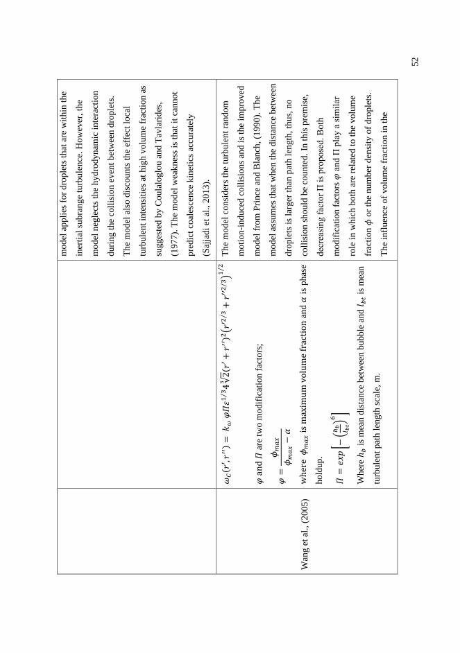
52
mo
del
appli
es f
or
dro
ple
ts t
hat
are
wit
hin
the
iner
tial
subra
ng
e tu
rbule
nce
. H
ow
ever
, th
e
mo
del
neg
lect
s th
e hyd
rody
nam
ic i
nte
ract
ion
du
rin
g t
he
coll
isio
n e
ven
t b
etw
een d
rople
ts.
The
mod
el a
lso
dis
counts
the
effe
ct l
oca
l
turb
ule
nt
inte
nsi
ties
at
hig
h v
olu
me
frac
tion a
s
sug
ges
ted
by
Co
ula
log
lou a
nd T
avla
rid
es,
(197
7).
The
mod
el w
eak
nes
s is
that
it
can
not
pre
dic
t co
ales
cen
ce k
inet
ics
accu
rate
ly
(Saj
jad
i et
al.
, 201
3).
Wan
g e
t al
., (
20
05
)
𝜔𝐶( 𝑟
′,𝑟
′′)=
𝑘𝜔 𝜑
𝛱1
3⁄
4√2
3( 𝑟
′+𝑟
′ ′)2
(𝑟′2
3⁄
+𝑟′
′23
⁄)1
2⁄
𝜑 a
nd 𝛱
are
tw
o m
odif
icat
ion
fac
tors
;
𝜑=
𝜙𝑚
𝑎𝑥
𝜙𝑚
𝑎𝑥
−𝛼
wher
e 𝜙
𝑚𝑎𝑥 is
max
imum
volu
me
frac
tion
an
d 𝛼
is
ph
ase
hold
up
.
𝛱=
𝑒𝑥𝑝
[−(
ℎ𝑏
𝑙 𝑏𝑡)6
]
Wh
ere ℎ
𝑏 i
s m
ean
dis
tance
bet
wee
n b
ub
ble
an
d 𝑙
𝑏𝑡 i
s m
ean
turb
ule
nt
pat
h l
ength
sca
le,
m.
The
mod
el c
onsi
der
s th
e tu
rbu
lent
ran
dom
mo
tion
-indu
ced c
oll
isio
ns
and i
s th
e im
pro
ved
mo
del
fro
m P
rince
and
Bla
nch
, (1
99
0).
Th
e
mo
del
ass
um
es t
hat
wh
en t
he
dis
tan
ce b
etw
een
dro
ple
ts i
s la
rger
th
an p
ath l
eng
th, th
us,
no
coll
isio
n s
ho
uld
be
cou
nte
d.
In t
his
pre
mis
e,
dec
reas
ing f
acto
r Π
is
pro
pose
d.
Bo
th
mo
dif
icat
ion
fac
tors
𝜑 a
nd
Π p
lay
a s
imil
ar
role
in w
hic
h b
oth
are
rel
ated
to
th
e volu
me
frac
tion 𝜙
or
the
nu
mb
er d
ensi
ty o
f dro
ple
ts.
The
infl
uen
ce o
f volu
me
frac
tion
in
the

53
pro
pose
d c
oll
isio
n f
requ
ency
is
ob
vio
us
and
imp
ort
ant,
how
ever
, th
e def
init
ion
of 𝜑
and Π
are
stil
l nee
ded
to
be
inves
tig
ated
thoro
ug
hly
(Lia
o a
nd L
uca
s, 2
010).
The
model
pre
dic
ts
smal
l co
llis
ion f
requ
ency
for
smal
l dro
ple
ts
bec
ause
th
e m
ean d
ista
nce
bet
wee
n s
mal
l
dro
ple
t is
lar
ger
th
an b
ig d
rople
ts i
f dro
ple
t
nu
mber
is
equ
al (
Lia
o a
nd L
uca
s, 2
00
9).
Th
e
mo
del
als
o d
oes
not
acco
unt
the
dam
pin
g
effe
ct p
ropose
d b
y C
ou
lalo
glo
u a
nd
Tav
lari
des
, (1
97
7)
for
hig
h t
urb
ule
nt
inte
nsi
ties
at
hig
h d
isper
sed f
ract
ion.
Car
rica
et
al.,
(1
999
)
𝜔𝐶( 𝑟
′,𝑟′
′)=
(3
10𝜋𝜈)1
2⁄
[(4𝜋𝑟
′3
3)
13
⁄
+(4𝜋𝑟
′′3
3)
13
⁄
]3
for ( 𝑟
′<
𝑙 𝑒;𝑟
′′<
𝑙 𝑒)
𝜔𝐶( 𝑟
′,𝑟′
′)=
5.6
13
⁄√2
3( 𝑑
′+
𝑑′′)2
𝑑′1
3⁄
for ( 𝑟
′<
𝑙 𝑒;𝑟
′′>
𝑙 𝑒)
The
mod
el i
s der
ived
fro
m t
he
turb
ule
nt-
ind
uce
d c
oll
isio
ns
and
only
bin
ary c
oll
isio
n
even
t is
consi
der
ed.
Th
e m
odel
is
pro
po
sed f
or
gas
-liq
uid
syst
em.
They
rep
ort
ed t
hat
duri
ng
coll
isio
n b
etw
een d
rop
lets
, co
ales
cen
ce m
ay
no
t h
app
en h
ow
ever
, m
om
entu
m t
ransf
er
bet
wee
n c
oll
idin
g d
rople
ts d
oes
occ
ur.
Hen
ce,
in r
egio
ns
wh
ere
gas
volu
me
frac
tion i
s h
igh
the
pre
sen
ce o
f su
rfac
tan
t ca
n i
nhib
it
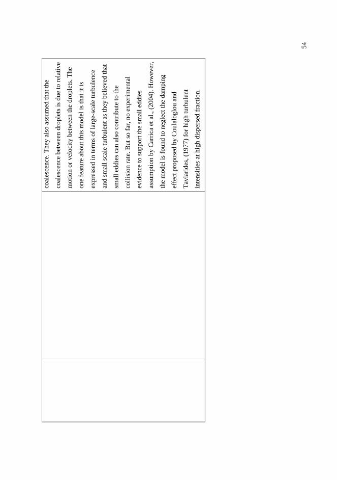
54
coal
esce
nce
. T
hey
als
o a
ssum
ed t
hat
the
coal
esce
nce
bet
wee
n d
rople
ts i
s du
e to
rel
ativ
e
mo
tion o
r vel
oci
ty b
etw
een t
he
dro
ple
ts.
The
on
e fe
atu
re a
bout
this
model
is
that
it
is
exp
ress
ed i
n t
erm
s of
larg
e-sc
ale
turb
ule
nce
and
sm
all
scal
e tu
rbule
nt
as t
hey
bel
ieved
that
smal
l ed
die
s ca
n a
lso
con
trib
ute
to t
he
coll
isio
n r
ate.
But
so f
ar,
no
ex
per
imen
tal
evid
ence
to s
up
port
the
smal
l ed
die
s
assu
mpti
on
by
Car
rica
et
al., (
2004).
Ho
wev
er,
the
model
is
fou
nd t
o n
egle
ct t
he
dam
pin
g
effe
ct p
ropose
d b
y C
ou
lalo
glo
u a
nd
Tav
lari
des
, (1
97
7)
for
hig
h t
urb
ule
nt
inte
nsi
ties
at
hig
h d
isper
sed f
ract
ion
.
55
2.4.2 Coalescence efficiency function, 𝝍𝑬(𝒓′, 𝒓′′)
The model for coalescence efficiency or coalescence probability is introduced due to
the fact that not all the droplets that collided coalesce and some fractions of the droplets are
found to be separated after the collisions. In general, coalescence efficiency models are
determined based on three major approaches namely energy model, critical velocity model,
and film drainage model (Liao and Lucas, 2010; Solsvik and Jakobsen, 2014).
2.4.2.1 The energy model
The coalescence efficiency model based on energy approach was first introduced by
Howarth in 1964 in his study on coalescence of droplets in a turbulent flow field. From the
model proposed, it was found that, the efficiency of coalescence significantly increases with
increasing energy of collision. Experimental evidence from Park and Blair, (1975) proved
that the coalescence is most likely to occur when the turbulence energy increased. To
express this phenomenon, Sovova, (1981) introduced the coalescence efficiency model that
incorporates with kinetic collision energy (𝐸𝑘) and surface energy (𝐸𝜎) as written below:
𝜓𝐸(𝑑, 𝑑′) = 𝑒𝑥𝑝 (−𝑘𝑐
𝐸𝜎
𝐸𝑘) (2.12)
From the expression in Eqn. (2.12) shows that the probability of coalescence (𝜓𝐸) from drop
collision increases if the kinetic collision energy is greater than the surface energy holding the
droplet together (i.e., 𝐸𝑘 > 𝐸𝜎). Simon, (2004) proposed coalescence efficiency model based
on similar principles as Sovova, (1981) but using momentum balance expression to determine
the kinetic energy during collision. Nevertheless, the model discounted the effect from the
drainage and rupture of intervening film between droplets.

56
2.4.2.2 The critical velocity model
On the other hand, the critical velocity model approach is developed based on the
opposite principles to the energy model approach. In this respect, the coalescence of droplets
is observed to favour gentle collisions instead of high velocity collisions as proposed in the
energy model (Liao and Lucas, 2010). In this model, the result of coalescence efficiency
mainly relies upon the approach velocity of the colliding droplets. Lehr et al., (2002)
proposed a simple expression to describe the coalescence efficiency in terms of critical
approach velocity in bubble columns as follows:
𝜓𝐸(𝑟, 𝑟′) = 𝑚𝑖𝑛 (𝑢𝑐𝑟𝑖𝑡
𝑢𝑟𝑒𝑙, 1) (2.13)
In Eqn. (2.13) above, the 𝑢𝑐𝑟𝑖𝑡 denotes the critical velocity and 𝑢𝑟𝑒𝑙 is the relative velocity
between the droplets. This model is considered empirical owing to the fact that 𝑢𝑐𝑟𝑖𝑡 has to be
determined experimentally.
2.4.2.3 The film drainage model
The film drainage model is the most accepted and widely used theory to determine the
coalescence efficiency and has become the reference for all subsequent models (Liao and
Lucas, 2010; Sajjadi et al., 2013). The film drainage model is developed based on two
characteristic time scales known as contact time, 𝑡𝑐𝑜𝑛𝑡𝑎𝑐𝑡 between colliding droplets and
drainage time, 𝑡𝑑𝑟𝑎𝑖𝑛𝑎𝑔𝑒 for the intervening film to reach the critical thickness and rupture.
To achieve coalescence, the collided drops must remain in contact for sufficient time until the
liquid film thins to its critical thickness. In short, the contact time must be longer than the
drainage time (𝑡𝑐𝑜𝑛𝑡𝑎𝑐𝑡 > 𝑡𝑑𝑟𝑎𝑖𝑛𝑎𝑔𝑒) for coalescence to occur as shown in Fig. 2.8 (Kamp et
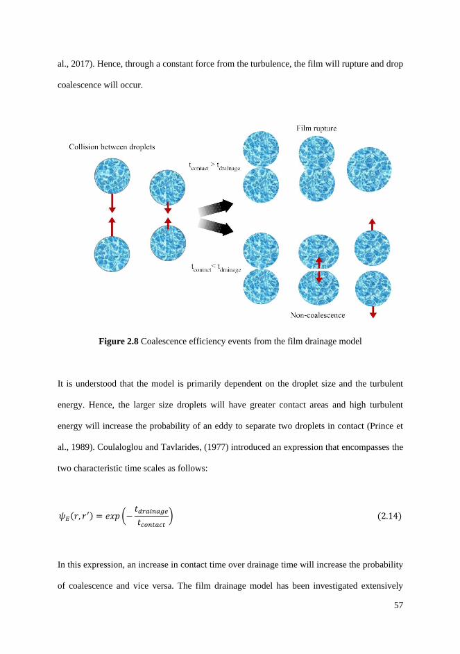
57
al., 2017). Hence, through a constant force from the turbulence, the film will rupture and drop
coalescence will occur.
Figure 2.8 Coalescence efficiency events from the film drainage model
It is understood that the model is primarily dependent on the droplet size and the turbulent
energy. Hence, the larger size droplets will have greater contact areas and high turbulent
energy will increase the probability of an eddy to separate two droplets in contact (Prince et
al., 1989). Coulaloglou and Tavlarides, (1977) introduced an expression that encompasses the
two characteristic time scales as follows:
𝜓𝐸(𝑟, 𝑟′) = 𝑒𝑥𝑝 (−𝑡𝑑𝑟𝑎𝑖𝑛𝑎𝑔𝑒
𝑡𝑐𝑜𝑛𝑡𝑎𝑐𝑡) (2.14)
In this expression, an increase in contact time over drainage time will increase the probability
of coalescence and vice versa. The film drainage model has been investigated extensively
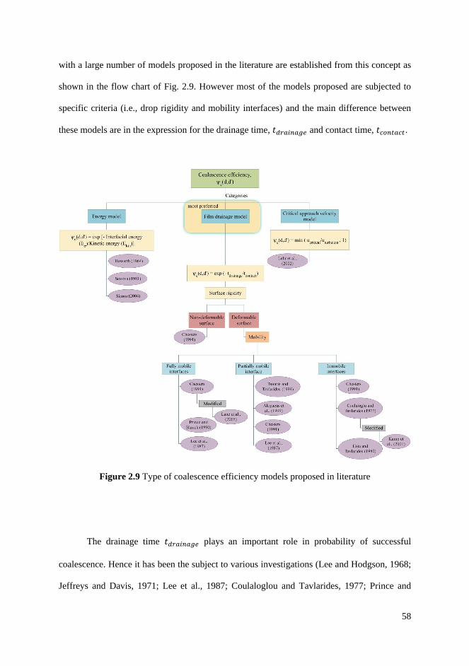
58
with a large number of models proposed in the literature are established from this concept as
shown in the flow chart of Fig. 2.9. However most of the models proposed are subjected to
specific criteria (i.e., drop rigidity and mobility interfaces) and the main difference between
these models are in the expression for the drainage time, 𝑡𝑑𝑟𝑎𝑖𝑛𝑎𝑔𝑒 and contact time, 𝑡𝑐𝑜𝑛𝑡𝑎𝑐𝑡.
Figure 2.9 Type of coalescence efficiency models proposed in literature
The drainage time 𝑡𝑑𝑟𝑎𝑖𝑛𝑎𝑔𝑒 plays an important role in probability of successful
coalescence. Hence it has been the subject to various investigations (Lee and Hodgson, 1968;
Jeffreys and Davis, 1971; Lee et al., 1987; Coulaloglou and Tavlarides, 1977; Prince and

59
Blanch, 1990; Tsouris and Tavlarides, 1994; Luo, 1993; Chesters, 1991; Saboni et al., 1995;
Simon, 2004; Lane et al., 2005). Most of the researchers agreed that in film drainage model
the drainage time 𝑡𝑑𝑟𝑎𝑖𝑛𝑎𝑔𝑒 depends on the rigidity of the droplet surfaces as well as mobility
of the contact interfaces (Lee and Hodgson, 1968; Chesters, 1991; Liao and Lucas, 2010;
Sajjadi et al., 2013; Abidin et al., 2015). Analytical solution for 𝑡𝑑𝑟𝑎𝑖𝑛𝑎𝑔𝑒 exist is only for the
case of non-deformable drops with immobile interfaces (Chesters, 1991). The contact time,
𝑡𝑐𝑜𝑛𝑡𝑎𝑐𝑡 is also important for the calculation of the coalescence time in a turbulent system.
There have been numerous studies and models proposed for the contact time in literature
(Schwartzber and Treybal, 1968; Chesters, 1991; Luo, 1993; Coulaloglou and Tavlarides,
1977; Kamp et al., 2001; Tsouris and Tavlarides, 1994) and most of the models developed
used the expression from Levich (1962) that are based on dimensional analysis.
2.4.2.3.1 Rigidity of droplet surfaces: non-deformable
The non-deformable droplets apply to the case where the droplets are far away from
each other or the droplets are physically small in size for instance, the drop size diameter,
𝑑 < 1.0 mm and the droplets have higher viscosity than the continuous phase (Simon, 2004,
Liao; Lucas, 2010). In this respect, the droplets are assumed to be spherically rigid and non-
deformable. Chesters (1991) proposed a model to describe the drainage time, 𝑡𝑑𝑟𝑎𝑖𝑛𝑎𝑔𝑒 under
these circumstances for two equal-sized droplets with non-deformable surfaces via the
Poiseuille relation. However, most researchers disagree with non-deformable surfaces theory
due to the fact that the model only applies for very small droplets (𝑑 < 1.0 mm) wherein
practically larger droplets also existed and should be considered during the collision (Simon,
2004).

60
2.4.2.3.2 Rigidity of droplet surfaces: deformable
Nearly all the film drainage models available in literature consider that the droplet
surfaces are deformable. This is true considering the droplets in real conditions are present in
the form of bigger and smaller sizes. Hence, deformable surfaces should be considered if one
is investigating the coalescence efficiency based on the film drainage model. Kamp et al.,
(2017) explained that the collision between two droplets mostly occurs with deformable
droplet surfaces as shown in Fig. 2.13 that subsequently resulted in coalescence. Liao and
Lucas, (2010) argued that the complex film drainage with deformable surfaces depends on
the mobility of the colliding interfaces. In this respect, the film drainage model can be
divided into three regimes known as the deformable droplet with immobile, partially mobile,
and fully mobile interfaces. These regimes are controlled by either inertial force dominate, or
viscous force dominate in the draining film (Chesters, 1991). In the case where highly
viscous dispersed phase is present in the liquid-liquid system, the drainage is mainly
dominated by viscous force.
The rigidity of the droplet surfaces can be classified into two categories namely,
deformable and non-deformable surfaces as shown in Fig. 2.10. While the mobility of the
contact interfaces is divided into three types such as immobile interfaces, partially mobile
interfaces, and fully mobile interfaces as depicted in Fig. 2.11 from Simon (2004) and Sajjadi
et al., (2013) and Fig. 2.12 from Lee and Hodgson, (1968). Analytical solution for 𝑡𝑑𝑟𝑎𝑖𝑛𝑎𝑔𝑒
exist only for the case of non-deformable drops with immobile interfaces (Chesters, 1991).

61
Figure 2.10 Rigidity of the droplet surfaces: (a) Non-deformable and (b) Deformable from
Simon, (2004) and Chesters, (1991).
(a) (b) (c)
Figure 2.11 Mobility of the droplet interfaces: (a) Immobile interfaces, (b) Partially mobile
interfaces, (c) Fully mobile interfaces, from Simon, (2004) and Sajjadi et al., (2013).

62
Figure 2.12 Mobility of the droplet interfaces at plane film (Lee and Hodgson, 1968): (a)
Immobile interfaces, (b) Partially mobile interfaces, and (c) Fully mobile interfaces. The
pressure distribution is shown at the top (a).
On the other hand, if the continuous phase has a low viscosity (i.e., inviscid), the
drainage is dominated by the inertial force where the film deformed due to acceleration and
continuous movements at the interfaces. Apart from that, in the deformable surfaces of the
droplets, Derjaguin and Kussakov (1939) found that there is a dimple on the surfaces which
indicates the presence of pressure gradient across the surfaces of the deformable droplets as
shown Fig. 2.11. In this respect, the film layer is not flat and needs to be converted to a
curved shape in order to accommodate the pressure gradient. However, due to simplicity,
most of the drainage models proposed in literature discounted the dimple but instead
considered a parallel (flat) model such that the thickness layer of liquid film is smaller than
the radius of the droplets (Kamp et al., 2017). From this assumption, several models have
been proposed while taking into account the mobility of the droplet interfaces.

63
Figure 2.13 Deformable surfaces of droplets (Kamp et al., 2017)
2.4.2.3.2.1 Interface mobility: deformable with immobile interfaces
Droplets with immobile interfaces are generally applied to systems with a very
viscous dispersed phase or systems with very specific surfactant soluble concentration in the
continuous phase (Saboni et al., 1995; Liao and Lucas, 2010). In this respect, the deformable
droplet with immobile interfaces (i.e., contact surfaces) is influenced by the viscous thinning
or thinning rate of the film. The contact surfaces can be another droplet, a wall or the
interface of the continuous fluid (Æther, 2002). According to Lee and Hodgson (1968), the
immobile interfaces mean that there is a sufficiently large surface shear stress existing to
oppose the viscous shear stress of the droplet or in other words, the droplet can support an
infinite high shear stress (Æther, 2002). This occurs due to the presence of surfactant or
impurities to immobilize the surface (Æther, 2002; Lee and Hodgson, 1968). The film at this
condition will drain very slowly in comparison to the fully mobile case (Æther, 2002). The
underlying theory for this model assumes that continuous flow in the liquid film is laminar
and the inertial effects are negligible (Tsouris and Tavlarides, 1994). No slip at the surface
and velocity profile as depicted in Fig. 2.11(a) indicates that the film is having maximum
velocity at the centre and no velocity at the contact surfaces. Furthermore, the forces at the
interfaces are assumed normal, hence, the Van der Waals, tangential, and double layer
stresses are all negligible. The interaction between the film drainage and the movement
64
within the particles are separated. Colaloglou and Tavlarides, (1977) presented thorough
synthesis of how coalescence occurs in liquid-liquid dispersion when the intervening liquid
film drains to a critical thickness with deformable droplets at immobile interfaces.
2.4.2.3.2.2 Interface mobility: deformable with partially mobile interfaces
Droplets with partially mobile interfaces are generally applied to the system with
intermediate viscosity, which is less than immobile case and greater than fully mobile case. It
can also apply to a system where the impurities or the surfactants are swept away from the
interfaces (Æther, 2002). In general, the drainage in liquid-liquid system is controlled by the
motion of the film surface. Hence, if there is a presence of additional flow within the film due
to prevailing pressure gradient being much smaller, the event is known as partially immobile
interfaces (Chesters, 1991; Æther, 2002). Since film drainage model for drops with partially
mobile interfaces is an intermediate case between immobile and fully mobile interfaces,
partial mobility can be considered complicated case due to the fact that the drainage process
is controlled by both inertia and viscous forces. Hydrodynamic force, 𝐹𝑦 and compressing
force, 𝐹𝑐 are introduced to describe the interaction forces at the contact surfaces between the
two droplets in terms of resisting (𝐹𝑦) and attracting (𝐹𝑐) forces. Both forces are assumed to
occur during the film drainage and play an important role to develop the expression for the
drainage time in terms of deformable drops with partially mobile interfaces and fully mobile
interfaces. Davis et al., (1989) approximated the interaction forces, 𝐹𝑦 and 𝐹𝑐 to determine the
drainage time, 𝑡𝑑𝑟𝑎𝑖𝑛𝑎𝑔𝑒 for drop with partially mobile interface and later employed by
Tsouris and Tavlarides, (1994). On the other hand, Chesters (1991) also proposed the film
drainage model for drops with partially mobile interfaces by assuming a quasi-steady
creeping flow and Lee et al., (1987) employed the model from Sagert and Quinn (1976) to
express the model for drops with partially mobile case.

65
2.4.2.3.2.3 Interface mobility: deformable with fully mobile interfaces
Deformable droplet with fully mobile interfaces is the case where the dispersed phase
having a very low viscosity (i.e., inviscid). In this respect, the drainage is no longer controlled
by the viscous stress as in partial mobility and immobile interfaces but instead by the
resistance occurred in the film due to deformation and acceleration (Chesters, 1991).
Therefore, the inertial forces are controlling the process of film drainage. As shown in Fig.
2.12 (c), the fully mobile has the uniform velocity profile which indicates that the film will
drain fast at this condition compared to immobile case (Æther, 2002). In general, Chesters,
(1991) and Chan et al., (2011) defined the deformable drops with fully mobile interfaces as a
shear-stress free case or when the surface could not withstand the shear stress and move with
the flow (Æther, 2002). In this respect, the system is either pure fluids (i.e., no impurities or
surfactants) or the surfactant and impurities are swept away from the interface from the
partial mobility. On the other hand, Davis et al., (1989) described the process to be influenced
by the viscous force and approximated the resisting hydrodynamic force for fully mobile
interfaces in terms of dispersed phase viscosity. Luo, (1993) proposed the film drainage
model from the inertia-controlled limit for the case involving gas bubbles in turbulent flow.
Chesters, (1991) proposed the drainage model by using the parallel-film model approach and
taking into account the both terms which is viscous and inertial stresses. Lee et al., (1987)
proposed the model for a system having a pure inviscid dispersed phase liquid (𝜇 < 10mPa.s)
and Prince and Blanch, (1990) suggested the improved model from Oolman and Blanch,
(1986) by discounting the Hamaker contribution due to the small influence on overall
coalescence time. Several numbers of coalescence efficiency models proposed in the
literature which are based on the three discussed mechanism are depicted in Table 2.4.

66
Ta
ble
2.4
Coal
esce
nce
eff
icie
ncy
fun
ctio
ns,
𝜓𝐸
Au
thors
C
oa
lesc
ence
eff
icie
ncy
fu
nct
ion
s, 𝝍
𝑬
Ass
essm
ent
of
the
mo
del
Coula
log
lu a
nd
Tav
lari
des
, (1
97
7)
𝜓𝐸( 𝑟
′,𝑟
′′)=
exp
[−𝑘
𝜓
16𝜇
𝑐𝜌
𝑐
𝜎2( 1
+𝜙
)3(
𝑟′𝑟
′′
𝑟′+
𝑟′′)
4
]
This
co
ales
cen
ce e
ffic
ien
cy m
odel
is
dev
elop
ed b
ased
on t
wo d
iffe
rent
char
acte
rist
ic t
ime
scal
es;
dra
inag
e ti
me
scal
es a
nd c
onta
ct t
ime
scal
es.
The
coal
esce
nce
is
assu
med
to o
ccu
r if
th
e
conta
ct t
ime
bet
wee
n t
wo d
rop
lets
is
long
er
than
th
innin
g t
ime
of
the
inte
rven
ing f
ilm
to
reac
h c
riti
cal
thic
kn
ess
or
refe
rred
to a
s
dra
inag
e ti
me
(con
tact
tim
e >
dra
inag
e
tim
e).
The
mo
del
als
o a
ssu
mes
that
the
dro
ple
t is
def
orm
able
wit
h i
mm
obil
e
inte
rfac
es.
Wh
ilst
th
e in
itia
l an
d c
riti
cal
film
thic
knes
s ar
e lu
mped
into
the
const
ant
par
amet
er. T
he
dra
inag
e ti
me
dev
elop
ed
bas
ed o
n m
ob
ilit
y o
f th
e co
llid
ing i
nte
rfac
e
(i.e
., i
mm
obil
e, p
arti
ally
mob
ile,
or
full
y
mo
bil
e). T
he
coal
esce
nce
tim
e fo
r m
obil
e
inte
rfac
es i
s sh
ort
er t
han
im
mob
ile
inte
rfac
e

67
(Liu
and L
i, 1
99
9).
The
inte
rfac
e m
ob
ilit
y
is a
ssoci
ated
wit
h s
urf
ace
ten
sio
n g
radie
nt
and v
isco
sity
of
the
dro
ple
ts, w
her
ein
incr
ease
in t
hes
e par
amet
ers
lead
s to
imm
ob
ilit
y o
f th
e in
terf
aces
and
dec
reas
es
the
coal
esce
nce
eff
icie
ncy
. T
he
mo
del
consi
der
s th
e d
ampin
g c
orr
ecti
on
fac
tor
(1+
𝜙)
to t
ake
into
acc
ount
the
hig
h
dis
per
sed
vo
lum
e fr
acti
ons.
Luo
, (1
993
)
𝜓𝐸( 𝑟
′,𝑟
′′)
=ex
p[−
𝑘𝜓
4𝑢
rel𝜌
𝑐𝑟
′2
𝜎( 1
+𝛿)3
√(0.7
5( 1
+𝛿
2)(
1+
𝛿3) 𝜎
8(𝜌
𝑑𝜌
𝑐⁄
+ 𝐶
𝑉𝑀)𝜌
𝑐𝑟′
3)]
Wher
e, 𝛿
= 𝑟
′𝑟′
′⁄
, 𝑢
rel=
2.4
11
2⁄
13
⁄√2
3(𝑟
23
⁄+
𝑟′2
3⁄
)12
⁄
The
mo
del
was
dev
elo
ped
bas
ed o
n
turb
ule
nt
rando
m m
oti
on
-in
duce
d c
oll
isio
ns
and f
ilm
dra
inag
e m
od
el.
Suit
able
fo
r both
par
tial
ly a
nd f
ull
y m
obil
e in
terf
aces
. L
uo,
(19
93)
crit
iciz
ed t
he
sim
pli
city
of
Lev
ich
(19
62)
expre
ssio
n a
nd s
uit
abil
ity f
or
uneq
ual
-siz
ed l
iqu
id d
rop
lets
as
adopte
d b
y
Ch
este
rs, (1
991
) in
his
co
ales
cen
ce
effi
cien
cy d
eriv
atio
n.
In t
his
pre
mis
e, L
uo,
(19
93)
der
ived
mo
re r
easo
nab
le a
nd
fun
dam
enta
l m
odel
for
the
inte
ract
ion
tim
e
bas
ed o
n s
imple
par
alle
l fi
lm m
odel
as

68
dep
icte
d i
n T
able
2.4
. H
e ad
ded
th
e m
ass
coef
fici
ent,
𝐶𝑉𝑀
of
the
dro
ple
ts i
n t
he
expre
ssio
n s
imil
ar t
o L
uo a
nd
Sven
dse
n
(19
96b
) m
odel
. H
ow
ever
, it
is
ob
serv
ed
that
𝐶𝑉𝑀
is
det
erm
ined
duri
ng t
he
appro
ach
pro
cess
(K
amp e
t al
., 2
00
1).
Acc
ord
ing t
o
the
work
by J
eela
ni
and
Har
tlan
d,
(1991
),
the
par
amet
er 𝐶
𝑉𝑀
is
no
rmal
ly t
aken
to b
e a
const
ant
bet
wee
n 0
.5 a
nd
0.8
.
Luo
and
Sv
end
sen
,
(199
6b
) an
d W
ang
et
al.,
(2
005
)
𝜓𝐸( 𝑟
′,𝑟
′′)=
exp
[−(0
.75( 1
+𝛿
2)(
1+
𝛿3) )
12
⁄
(𝜌𝑑
𝜌𝑐
⁄+
𝐶𝑉𝑀)(
1+
𝛿)3
𝑊𝑒 𝑑
′𝑑′′
12
⁄]
Wher
e, 𝛿
= 𝑟
′𝑟′
′⁄
and
𝐶𝑉𝑀
is
the
vir
tual
mas
s co
effi
cien
t.
The
mo
del
is
bas
ed o
n e
ner
gy c
on
serv
atio
n
appro
ach a
nd
a c
onti
nuo
us
work
of
Luo
,
(19
93).
Th
e fu
nct
ion a
ssum
es t
hat
th
e
iner
tial
coll
isio
n i
s ca
use
d b
y t
urb
ule
nt
fluct
uat
ion
s an
d t
hey
are
der
ived
bas
ed o
n
iso
tro
pic
turb
ule
nce
. T
he
dro
ple
t co
nta
ct
tim
e w
as c
alcu
late
d b
ased
on e
ner
gy
conse
rvat
ion d
uri
ng d
rop
let
coll
isio
n.
Th
e
mo
del
was
dev
eloped
on
bas
is o
f gas
-liq
uid
flow
and
acc
ou
nts
th
e ef
fect
of
film
dra
inag
e. T
hey
ass
um
ed t
hat
th
e ti
me
for
the
film
are
a to
go f
rom
zer
o t
o i
ts

69
max
imum
equ
als
the
tim
e fo
r th
e re
ver
se
pro
cess
bac
k t
o z
ero a
nd t
his
ind
icat
es t
hat
the
inte
ract
ion
tim
e n
ot
only
dep
end
s on
th
e
fluid
pro
per
ties
, but
also
on t
he
radiu
s ra
tio
of
the
two a
pp
roac
hin
g d
rop
lets
or
bubb
les.
The
mo
del
show
s a
go
od
abil
ity
to
pre
dic
t
dro
p d
istr
ibuti
on
.
Lan
e et
al.
, (2
00
5)
𝜓𝐸( 𝑟
)=
exp
(−
0.7
1√
25
3⁄
𝜌𝑐
23
⁄𝑟
53
⁄
𝜎)
×
exp
(−
5.4
9×
10
6×
8𝑟
3
)
The
mo
del
is
the
imp
roved
ver
sion f
rom
Ch
este
rs, (1
991
) an
d P
rin
ce a
nd
Bla
nch
(19
90).
Th
e m
odel
is
dev
elo
ped
on t
he
bas
is t
hat
the
rate
of
bin
ary c
oll
isio
ns
bet
wee
n d
rople
ts m
ovin
g w
ith a
ran
dom
vel
oci
ty e
qual
to
the
turb
ule
nt
fluct
uat
ing
vel
oci
ty o
f ed
die
s of
the
sam
e si
ze w
ithin
the
iner
tial
subra
ng
e. T
he
mod
el a
lso
acco
un
ts t
he
finit
e ti
me
for
dro
ple
t
def
orm
atio
n a
nd
fil
m d
rain
age.
Acc
ord
ing
to L
ane
et a
l., (2
00
5),
th
e m
odel
by
Ch
este
rs, (1
991
) neg
lect
ed t
he
min
imum
ener
gy r
equir
ed f
or
dro
ple
t def
orm
atio
n a
nd
the
mo
del
by
Pri
nce
and B
lanch
(1
99
0)
did
70
not
pro
ve
sati
sfac
tory
wh
en a
ppli
ed t
o t
he
stir
red
tan
k s
imu
lati
ons,
sin
ce t
he
mod
el
lead
to
su
bst
anti
al c
oal
esce
nce
rat
es i
n t
he
bulk
of
the
tan
k, aw
ay f
rom
the
imp
elle
r.
Hen
ce, th
ey h
ave
impro
ved
the
coal
esce
nce
effi
cien
cy m
odel
an
d s
ug
ges
ted i
n t
he
mo
del
to a
ccoun
t fo
r th
e m
inim
um
lev
el o
f
turb
ule
nt
ener
gy t
hat
may
aff
ecti
ng
the
coal
esce
nce
eff
icie
ncy
as
wel
l as
the
neg
lig
ible
coal
esce
nce
in
the
bulk
of
the
tank
th
at w
as o
ver
look
ed b
y t
he
model
by
Pri
nce
an
d B
lan
ch (
1990
). T
hey
als
o
counte
d t
he
dro
ple
t vo
lum
e as
the
amou
nt
of
ener
gy
pro
du
ced a
ffec
ted b
y t
he
dro
p
volu
me.
The
mod
el w
as d
evel
oped
fo
r
equal
-siz
ed b
ub
ble
s fo
r g
as-l
iqu
id s
yst
em.
The
mo
del
was
pro
pose
d f
rom
ener
gy
mo
del
(w
her
e th
e p
rob
abil
ity o
f im
med
iate
coal
esce
nce
du
e to
sig
nif
ican
t co
llis
ion
incr
ease
s w
ith i
ncr
ease
in t
he
ener
gy o
f
coll
isio
n).
Th
e ex
pre
ssio
n o
f th
is m
odel
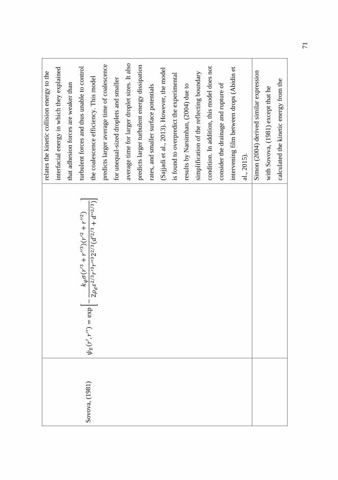
71
So
vov
a, (
1981)
𝜓𝐸( 𝑟
′,𝑟
′′)=
exp
[−𝑘
𝜓𝜎( 𝑟
′3+
𝑟′′
3)(
𝑟′2
+𝑟
′′2)
2𝜌
𝑑2
3⁄
𝑟′3𝑟
′′32
23
⁄( 𝑑
′23
⁄+
𝑑′′
23
⁄)]
rela
tes
the
kin
etic
coll
isio
n e
ner
gy t
o t
he
inte
rfac
ial
ener
gy
in
wh
ich t
hey
exp
lain
ed
that
adhes
ion f
orc
es a
re w
eaker
th
an
turb
ule
nt
forc
es a
nd
thus
un
able
to
contr
ol
the
coal
esce
nce
eff
icie
ncy
. T
his
mo
del
pre
dic
ts l
arger
av
erag
e ti
me
of
coal
esce
nce
for
un
equal
-siz
ed d
rople
ts a
nd s
mal
ler
aver
age
tim
e fo
r la
rger
dro
ple
t si
zes.
It
also
pre
dic
ts l
arger
turb
ule
nt
ener
gy d
issi
pat
ion
rate
s, a
nd s
mal
ler
surf
ace
pote
nti
als
(Saj
jadi
et a
l., 2
013
). H
ow
ever
, th
e m
od
el
is f
oun
d t
o o
ver
pre
dic
t th
e ex
per
imen
tal
resu
lts
by N
arsi
mh
an, (2
004)
due
to
sim
pli
fica
tio
n o
f th
e re
flec
ting b
ou
ndar
y
condit
ion
. In
add
itio
n,
this
mod
el d
oes
not
consi
der
th
e dra
inag
e an
d r
uptu
re o
f
inte
rven
ing
fil
m b
etw
een
dro
ps
(Abid
in e
t
al., 2
015).
Sim
on (
20
04)
der
ived
sim
ilar
expre
ssio
n
wit
h S
ovo
va,
(19
81
) ex
cept
that
he
calc
ula
ted t
he
kin
etic
ener
gy
fro
m t
he

72
Sim
on
, (2
004
)
𝜓𝐸( 𝑟
′,𝑟
′′)=
exp
[−4𝑘
𝜓𝜎( 𝑟
′2+
𝑟′′
2)
𝜌𝑑
23
⁄2
11
3⁄
( 𝑟′1
13
⁄+
𝑟′′
11
3⁄
)]
mo
men
tum
bal
ance
duri
ng
the
coll
isio
n.
The
mo
del
was
dev
elo
ped
bas
ed o
n t
he
pre
mis
e o
f en
erg
y m
od
el a
pp
roac
h w
hic
h i
s
sim
ilar
to t
he
work
of
So
vova
(1981
) an
d
Ch
atzi
et
al., (
198
9).
Th
e m
odel
ass
um
ed
that
th
e in
terf
acia
l en
erg
y o
f dro
ps
is
pro
port
ion
al t
o d
rop
surf
ace
area
and
inte
rfac
ial
ten
sio
n. T
he
kin
etic
co
llis
ion
ener
gy i
s pro
port
ional
to t
he
rela
tive
vel
oci
ty o
f tw
o c
oll
idin
g d
rops
and t
hei
r
aver
age
volu
me
(Sov
ova,
19
81).
Ho
wev
er,
the
kin
etic
coll
isio
n e
ner
gy
can
als
o b
e
det
erm
ined
fro
m t
he
mo
men
tum
bal
ance
duri
ng t
he
coll
isio
n o
f dro
ple
ts a
s su
gges
ted
by S
imon, (2
004)
in h
is c
oal
esce
nce
effi
cien
cy m
odel
. T
his
mo
del
is
not
appli
cable
fo
r lo
w t
urb
ule
nce
and b
ig
dro
ple
ts w
her
e th
e ti
mes
cale
s of
coll
isio
n
and c
oal
esce
nce
are
not
anal
ogou
s (S
ajja
di
et a
l.,
201
3).

73
Ches
ters
, (1
99
1)
𝜓𝐸( 𝑟
′ ,𝑟′
′)=
exp
[−𝑘
𝜓
25
6⁄
𝜌𝑐1
2⁄
13
⁄𝑟 𝑒
𝑞56
⁄
𝜎1
2⁄
]
𝑤ℎ𝑒𝑟
𝑒 𝑟
𝑒𝑞
=(1 𝑟′
+1 𝑟′′)−
1
The
mo
del
was
dev
elo
ped
bas
ed o
n f
ilm
dra
inag
e co
nce
pt
for
def
orm
able
dro
ple
t
wit
h f
ull
y m
obil
e in
terf
aces
. T
he
model
is
der
ived
bas
ed o
n s
imil
ar c
on
cept
of
film
dra
inag
e ev
ent
as C
oula
loglo
u a
nd
Tav
lari
des
(19
77
) ex
cept
on t
he
mob
ilit
y o
f
the
dro
ple
t in
terf
aces
. T
he
model
is
dev
elop
ed f
or
a li
quid
-liq
uid
sy
stem
wit
h
less
vis
cous
fluid
s (i
.e.,
inv
isci
d l
iquid
).
The
dra
inag
e m
odel
is
der
ived
fro
m t
he
iner
tial
ter
ms
in w
hic
h t
he
model
ass
um
ed
that
th
e vis
cosi
ty i
s su
ffic
ientl
y s
mal
l,
hen
ce d
rain
age
is n
o l
on
ger
con
troll
ed b
y
the
vis
cosi
ty b
ut
by
the
resi
stan
ce o
ffer
ed
by t
he
film
to d
efo
rmat
ion a
nd a
ccel
erat
ion
.
This
model
su
gg
este
d t
hat
the
dra
inag
e
tim
e fo
r th
e in
erti
a th
innin
g i
s pro
port
ional
to t
he
appro
ach v
elo
city
. T
his
indic
ates
that
if d
rain
age
tim
e is
sm
all,
the
coal
esce
nce
effi
cien
cy i
s h
igh,
thu
s th
e ap
pro
ach
vel
oci
ty i
s lo
w (
Lia
o a
nd
Luca
s, 2
01
0).

74
2.5 Energy dissipation rate
The turbulence kinetic energy dissipation rate, is an important property in turbulent
flow at high Reynolds number as it controls the drop breakup, heat transfer and mass transfer
(Wang et al, 2020). The rate of the dissipation is associated with the turbulent eddies in the
fluid flow or in brief, the strength of turbulence. Ideally, the dissipation rate, indicates the
rate at which the turbulence energy is absorbed, redistributed and transferred in the
fluctuating flow by breaking the eddies into smaller scales in cascade process driven by
vortex. In general, there are three different regions or energy flow of the turbulent energy
cascade. The length scale of the largest eddy is referred to the region of energy-containing
range. Instead, the smallest scale at which the eddies are dissipated by the viscous force and
converted into heat is denoted as to the region of dissipation range (viscous effect is
dominant). If the viscous effects are negligible, the eddies are suggested to be in inertial
subrange. There are various energy dissipation rates have been proposed in the literature
based on different turbulent conditions as depicted in Table 2.5.(Azizi and Taweel, 2011;
Raikar et al., 2009; Galinat et al., 2005; Jakobsen, 2014; Hesketh et al., 1991).
Table 2.5 Turbulent dissipation rate, from literature
Author Energy dissipation rate, 𝜺 Descriptions
Galinat et al. (2005) =
1
𝜌𝑐
∆𝑃𝑚𝑎𝑥𝑈
2𝐷(
1
𝛽2− 1)
Where, 𝛽 =𝐷𝑜
𝐷
The model is developed
based on the relation between
dissipation rate and
maximum pressure drop
across the orifice
∆𝑃𝑚𝑎𝑥 (pipe flow with
restriction) as well as the
orifice-pipe ratio, 𝛽.
Azizi and Taweel (2011) =
𝑈∆𝑃
𝜌𝑐𝐿𝑀
The rate of energy

75
dissipation proposed from the
pressure drop, ∆𝑃 in the
static mixer.
Hesketh et al. (1991) =
2𝑣𝑐3𝑓
𝐷
Where 𝑓 is from the Blasius
relation friction factor.
The energy dissipation rate is
calculated based on the
widely used empirical
relationship in turbulent pipe
flow. The friction factor, 𝑓 is
used for pressure drop in the
system.
Raikar et al. (2009) =
𝑐𝑃3 2⁄
𝑉1 3⁄ 𝜌𝑑−3 2⁄
Where 𝑃 is the
homogenization pressure and
𝑐 is constant.
The estimate is modified
from Coulaloglou and
Tavlarides (1977) for
emulsion in high pressure
homogeneizer.
Flórez-orrego et al. (2012) = 0.0176
𝑈3𝑅𝑒−3 8⁄
𝐷
The energy dissipation rate is
proposed from 𝜅 − model.
The turbulence assumed to
be generated from the bulk.
Jacobi, (2014) modified the estimate of the energy dissipation rate, , based on the
relationship between Reynolds number equation and friction factor, 𝑓 in the global specific
energy dissipation rate as follows:
≈2𝑣𝑙
3𝑓
𝐷≈
2𝑅𝑒3𝜈4𝑓
𝐷4≈ 0.16𝑅𝑒2.75 (
𝜈3
𝐷4) (2.15)
Where 𝑓 in equation 2.15 is fanning friction factor. The relation for the turbulent dissipation
energy is based on the wall friction as the primary source of turbulence production and is the
extended version from Hesketh et al. (1991). The turbulent dissipation energy can also be
76
derived from the 𝜅 − model as suggested by Flórez-orrego et al. (2012). However, this
estimate is only valid in the bulk as there are hardly any production of turbulence in the bulk,
thus the 𝜅 − model length scale gives very minimum turbulence. Nevertheless, estimation
of turbulent dissipation rate in turbulent multiphase flows is still limited (Wang et al., 2020).
In the following section, an overview of the available and popular approaches for PBE
solution are elucidated.
2.6 Solution to population balance equation (PBE)
This section offers an insight into several challenges as well as approaches employed
by other researchers in the literature as an effort to solve the complex PBE. For a liquid-
liquid flow in pipes, the droplet size distribution can affect significantly the rheological
behaviour and the pressure gradient of the fluids (Arirachakaran et al., 1989). Hence, a good
model that could accurately predict the drop size distribution in liquid-liquid emulsion is
crucial, particularly in processes related to separation application (Schümann, 2016).
Population balance equations (PBE) can be used to model and describe the complex case of
dynamic evolution of drop size distribution in pipe flow. The PBE are also represent the
transport equation for number density function of the droplets (Nguyen et al., 2016). In
general, to solve the PBE, one must discretize the particle volume domain into a number of
discrete elements. The resulting solutions will be in the form of stiff, nonlinear differential
and/or algebraic equations that are subsequently integrated numerically (Alexopoulos et al.,
2004). It is of interest to mention here that, there are many challenges involved in solving
PBE such as numerical complications, large number of equations involved, modeling
accuracy, computational efficiency, growth rate of the droplet due to breakage and
coalescence, inconsistency of droplet distribution in terms of size and time, as well as the
mechanism attributed to the drop size evolution (Rehman and Qamar, 2014; Pinar et al.,

77
2015; Korovessi and Linninger, 2005; Gunawan et al., 2004). According to Mesbah et al.,
(2009), the numerical solutions of PBE can be complicated due to the occurrence of sharp
discontinuities and steep moving fronts that result from convective nature of partial
differential equations as well as initial and boundary conditions incompatibility.
In recent years, there have been numerous methods proposed in literature to solve the
PBE (Kumar et al., 2008; Omar and Rohani, 2017). These include finite volume methods,
finite element methods, finite difference method, method of characteristics, moments method,
least-squares method, and Monte-Carlo method (see details in the review article by Vikas et
al., 2013; Kumar et al., 2008; Mesbah et al., 2009; Omar and Rohani, 2017; Solsvik et al.,
2013). The finite volume method was originally established for gas dynamics and presently it
has been adopted to solve the PBE (Qamar and Wernecke, 2007). It includes the
discretization of the spatial domain and uses piecewise functions to approximate the
derivatives (Mesbah et al., 2009). The resulting ordinary differential equations (ODE) will be
integrated over time (see details in Vikas et al., 2013; Gunawan et al., 2004; Qamar and
Wernecke, 2007). The finite element method involves the conversion from partial differential
equations (PDE) into algebraic equations for steady state and ODE for dynamic state (Omar
and Rohani, 2017). The final result in the form of stiff nonlinear differential equations is
integrated over time (see details in Alexopoulos et al., 2004; Rigopoulos and Jones, 2003).
However, this method may experience numerical complications due to the incompatibility
between the initial condition and boundary condition that cause moving discontinuity in
numerical solutions (Mesbah et al., 2009). In finite difference method, the differential
equations in PBE are approximated by difference equations in which implicit, explicit, and
Crank-Nicolson schemes are commonly used (Omar and Rohani, 2017). According to John
and Suciu (2014), the finite difference method will lead to nonphysical oscillations and

78
accuracy may have to compromise with computational cost (see details in Bennet and
Rohani, 2001; John and Suciu, 2014).
Kumar and Ramkrishna (1997) proposed method of characteristic to enhance the
solution accuracy of the discretized PBE. In this method, the PDE are transformed into ODE
by finding curves in the internal coordinate and time planes (i.e., 𝐿-𝑡 plane) resulting in
significant improvement of solution accuracy (Gunawan et al., 2004; Mesbah et al., 2009).
However, there are limitations involve of using this method in terms of long calculation times
for complex case and practical system, time-step selections, and obligated scalar modelling
(Lim et al., 2002) – see details in Lim et al., (2002) and Kumar and Ramkrishna (1997).
Hulburt and Katz (1964) are among the first who introduced the method of moments and the
main focus is to convert the PDE into ODE using a moment transformation. In this respect
the PBE are converted into moment equations of the number density (Omar and Rohani,
2017). There are various other subsequent models developed based on this method for
instance, quadrature method of moments, direct quadrature method of moments, sectional
quadrature method of moments, and extended quadrature method of moments (see details in
McGraw, 1997; Marchisio and Fox, 2005; Attarakih et al., 2009; Yuan et al., 2012; Akinola
et al., 2013). However, for complex systems the moment closure conditions are violated,
applicable to limited number of problems and no available information about the shape of the
distribution (Dorao and Jakobsen, 2006a; Gunawan et al., 2004; Omar and Rohani, 2017).
Another way of solving the PBE is by employing the least-squares method. The fundamental
idea of least-squares method is to minimize the integral of the square of the residual over the
computational domain (Dorao and Jakobsen, 2006a; 2006b). In this respect, the minimization
is performed for the norm-equivalent functional (see details in Solsvik et al., 2013; Dorao and
Jakobsen, 2006b; Zhu et al., 2008).

79
The least-square method is a well-established technique for solving various
mathematical problems and details of this method are discussed by Jiang (1998) and Bochev
and Gunzburger, (2009). However, in a system with high non-linearity and large scale, an
error occurred in the properties of the distribution and the method becomes unstable (Omar
and Rohani, 2017; Zhu et al., 2008). To address these issues, Zhu et al., (2008) introduced
least-squares method with direct minimization method. Still, the method does not always
produce a symmetric and positive-definite system (Omar and Rohani, 2017). Monte-Carlo
method solves the PBE by generating a set of solutions from randomly generated numbers in
the mathematical system (Omar and Rohani, 2017). To increase the accuracy of the system, a
greater number of randomly generated input trials is needed, and many individual droplets
must be tracked. In this regard, the method becomes computationally expensive (Nguyen et
al., 2016; Kumar et al., 2008; Gunawan et al., 2004). Monte-Carlo method is suitable for a
multi-dimensional and stochastic PBE particularly in a complex system (Kumar et al., 2008;
Ramkrishna, 1985). Although a plethora of studies have been conducted on numerical
solutions for PBE, robust solutions are still needed because more advanced control and
optimization strategies can be developed (Omar and Rohani, 2017).
2.7 Chapter summary
In this chapter the introduction and the importance of PBE in modeling the liquid-liquid
drops evolution is elucidated. In addition, the sub-processes for the population balance
equations in terms of breakage and coalescence models are also reviewed and discussed. The
underlying mechanisms for breakage frequency, daughter size distributions, coalescence
frequency, and coalescence efficiency are also reviewed. Details of method employed are
discussed in the following section.

80
CHAPTER 3
3 MODELING AND SIMULATION SETUP
3.1 Physical descriptions of the model
In turbulent dispersion of liquid-liquid systems, the fluid dynamics and the processes
involving particularly breakage and coalescence are complex. The simplist model for the
dynamic evolution of the drop density distribution of a liquid-liquid dispersion in turbulent
pipe flow system should assume isotropic turbulence with a uniform (plug) velocity, 𝑈 as
shown in Fig. 3.1 across pipe diameter, 𝐷 and length, 𝐿. This is a reasonable assumption
considering that the fine-scale structure in most of non-isotropic turbulent flows is found to
be locally close to isotropic (Hinze, 1959). Furthermore, isotropic turbulence assumption has
often been used for liquid-liquid dispersion studies (Coulaloglou and Tavlarides, 1977;
Tsouris and Tavlarides, 1994; Azizi and Tawell, 2011).
Figure 3.1 Sketch of turbulent flow field of a moving fluid in a pipe of length 𝐿, diameter 𝐷,
and moving with an average velocity (plug flow), 𝑈
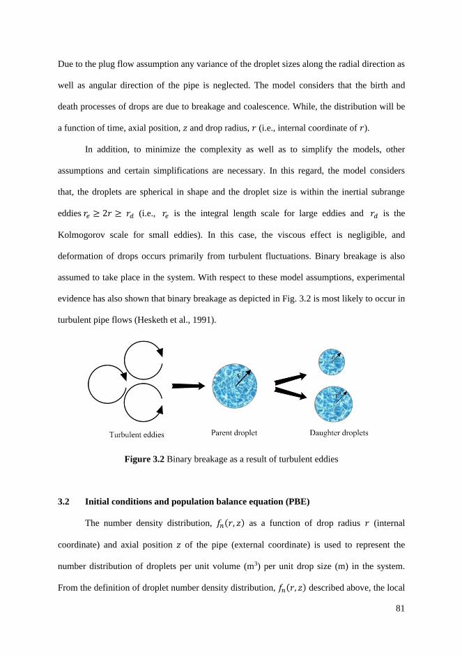
81
Due to the plug flow assumption any variance of the droplet sizes along the radial direction as
well as angular direction of the pipe is neglected. The model considers that the birth and
death processes of drops are due to breakage and coalescence. While, the distribution will be
a function of time, axial position, 𝑧 and drop radius, 𝑟 (i.e., internal coordinate of 𝑟).
In addition, to minimize the complexity as well as to simplify the models, other
assumptions and certain simplifications are necessary. In this regard, the model considers
that, the droplets are spherical in shape and the droplet size is within the inertial subrange
eddies 𝑟𝑒 ≥ 2𝑟 ≥ 𝑟𝑑 (i.e., 𝑟𝑒 is the integral length scale for large eddies and 𝑟𝑑 is the
Kolmogorov scale for small eddies). In this case, the viscous effect is negligible, and
deformation of drops occurs primarily from turbulent fluctuations. Binary breakage is also
assumed to take place in the system. With respect to these model assumptions, experimental
evidence has also shown that binary breakage as depicted in Fig. 3.2 is most likely to occur in
turbulent pipe flows (Hesketh et al., 1991).
Figure 3.2 Binary breakage as a result of turbulent eddies
3.2 Initial conditions and population balance equation (PBE)
The number density distribution, 𝑓𝑛(𝑟, 𝑧) as a function of drop radius 𝑟 (internal
coordinate) and axial position 𝑧 of the pipe (external coordinate) is used to represent the
number distribution of droplets per unit volume (m3) per unit drop size (m) in the system.
From the definition of droplet number density distribution, 𝑓𝑛(𝑟, 𝑧) described above, the local

82
total number density function, 𝑁𝑑(𝑧) and the local volume fraction, 𝜙(𝑧), of the dispersed
phase at a particular position of 𝑧 coordinate can be written as follows, respectively:
𝑁𝑑(𝑧) = ∫ 𝑓𝑛
∞
0
(𝑟′, 𝑧)𝑑𝑟′ (3.1)
𝜙(𝑧) = ∫ (4𝜋
3𝑟′3) 𝑓𝑛(𝑟′, 𝑧)𝑑𝑟′
∞
0
(3.2)
In Eqn. (3.2) above, 𝜙(𝑧) remains constant across the length of the pipeline since no drop
volume is gained or lost from coalescence or breakage and the volume is conserved. It is
worth noting that, using the drop volume, 𝑣, the number density distribution 𝑓𝑛 can be
converted to the volume density distribution, 𝑓𝑣, as follows:
𝑓𝑣(𝑟, 𝑧) = 𝑣𝑓𝑛(𝑟, 𝑧) = (4𝜋
3𝑟3)𝑓𝑛(𝑟, 𝑧) (3.3)
Apart from that, by taking into account the process of birth and death by breakage and
coalescence on the overall droplet growth processes, PBE for locally isotropic turbulent field
can be written as follows:
𝜕𝑓𝑛𝜕𝑡
= 𝑅𝐶𝑏(𝑟, 𝑡) − 𝑅𝐶𝑑
(𝑟, 𝑡) + 𝑅𝐵𝑏(𝑟, 𝑡) − 𝑅𝐵𝑑
(𝑟, 𝑡) (3.4)
By assuming isotropic turbulence with a uniform (plug) velocity, 𝑈 in pipe flow. The
expression in Eqn. (3.4) can be converted to rate of change of concentration of drops of
radius 𝑟 with axial position, 𝑧 as follows:

83
𝑈𝜕𝑓𝑛𝜕𝑧
= 𝑅𝐶𝑏(𝑟, 𝑧) − 𝑅𝐶𝑑
(𝑟, 𝑧) + 𝑅𝐵𝑏(𝑟, 𝑧) − 𝑅𝐵𝑑
(𝑟, 𝑧) 𝑓𝑜𝑟 0 ≤ 𝑧 ≤ 𝐿 , 0 ≤ 𝑟 ≤ ∞ (3.5)
In the Eqn. (3.5), 𝑅𝐶𝑏 and 𝑅𝐶𝑑 denote the birth and death rates of a droplet with radius 𝑟 due
to coalescence. While, 𝑅𝐵𝑏 and 𝑅𝐵𝑑 both represent the birth and death rates with radius 𝑟 due
to breakage, respectively.
The inlet (𝑧 = 0) number density function is, 𝑓𝑛0 and is given as:
0 ≤ 𝑧 ≤ 𝐿 , 0 ≤ 𝑟 ≤ ∞ , and 𝑓𝑛(𝑟, 𝑧 = 0) = 𝑓𝑛0(𝑟, 𝑧 = 0)
3.3 Coalescence birth and death functions
As volume is conserved in the coalescence process, the volumes of the parent droplets
(i.e., volume of the colliding particles) must equal to the volume of droplet formed. In this
respect, the radius, 𝑟′′, of the second parent droplet is constrained by the radius, 𝑟, of the
droplet formed and the radius, 𝑟′, of the first parent droplet. The relationship between the
merger of primary parent droplet which is having radius of 𝑟′ with a secondary parent
droplet of 𝑟′′ and the formation of new droplet, 𝑟 can be expressed as follows:
𝑟′′ = (𝑟3 − 𝑟′3)1 3⁄ (3.6)
Therefore, based on these definitions and relationships, the coalescence birth rate as a
function of drop radius, 𝑟 and axial position, 𝑧 is then given by:
𝑅𝐶𝑏(𝑟, 𝑧) = ∫ 𝑟𝑐(𝑟
′, 𝑟′′)𝑓𝑛(𝑟′, 𝑧)𝑓𝑛(𝑟′′, 𝑧)𝑟2
𝑟′′2𝑑𝑟′
𝑟 √23⁄
0
(3.7)

84
In the above equation (i.e., Eqn. 3.7), 𝑟𝑐 represents the volume rate of coalescence and is the
product between the collision frequency, 𝜔𝑐(𝑟′, 𝑟′′ ) and the coalescence efficiency,
𝜓𝑒(𝑟′, 𝑟′′ ) for drops having sizes of 𝑟′ and 𝑟′′. These two functions physically mean that two
droplets will coalesce when they are in collision. Therefore, the volume rate of coalescence 𝑟𝑐
can be written as follows:
𝑟𝑐(𝑟′, 𝑟′′ ) = 𝜔𝑐(𝑟
′, 𝑟′′ )𝜓𝑒(𝑟′, 𝑟′′ ) (3.8)
By taking into consideration the volume conservation in coalescence process, the parent
droplets lost (death) from the birth of droplets by coalescence must be accounted for.
Therefore, the death rate function from coalescence of parent droplets having radius 𝑟 is
given by:
𝑅𝐶𝑑(𝑟, 𝑧) = 𝑓𝑛(r, z)∫ 𝑟𝑐(𝑟, 𝑟
′)𝑓𝑛(𝑟′, 𝑧)∞
0
𝑑𝑟′ (3.9)
Both Eqns. (3.7) and (3.9) are valid under conditions of, 0 ≤ 𝑧 ≤ 𝐿 , 0 ≤ 𝑟 ≤ ∞.
3.4 Breakage birth and death functions
The death rate of a droplet having radius 𝑟 due to breakage can be determined by the
product of the breakage frequency, 𝑔(𝑟) and number density function, 𝑓𝑛(𝑟, 𝑧) as follows:
𝑅𝐵𝑑(𝑟, 𝑧) = 𝑔(𝑟)𝑓𝑛(𝑟, 𝑧) (3.10)
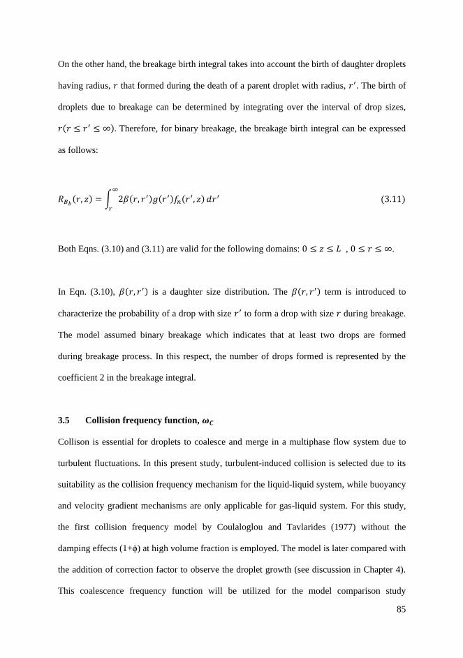
85
On the other hand, the breakage birth integral takes into account the birth of daughter droplets
having radius, 𝑟 that formed during the death of a parent droplet with radius, 𝑟′. The birth of
droplets due to breakage can be determined by integrating over the interval of drop sizes,
𝑟(𝑟 ≤ 𝑟′ ≤ ∞). Therefore, for binary breakage, the breakage birth integral can be expressed
as follows:
𝑅𝐵𝑏(𝑟, 𝑧) = ∫ 2𝛽(𝑟, 𝑟′)𝑔(𝑟′)𝑓𝑛(𝑟′, 𝑧)
∞
𝑟
𝑑𝑟′ (3.11)
Both Eqns. (3.10) and (3.11) are valid for the following domains: 0 ≤ 𝑧 ≤ 𝐿 , 0 ≤ 𝑟 ≤ ∞.
In Eqn. (3.10), 𝛽(𝑟, 𝑟′) is a daughter size distribution. The 𝛽(𝑟, 𝑟′) term is introduced to
characterize the probability of a drop with size 𝑟′ to form a drop with size 𝑟 during breakage.
The model assumed binary breakage which indicates that at least two drops are formed
during breakage process. In this respect, the number of drops formed is represented by the
coefficient 2 in the breakage integral.
3.5 Collision frequency function, 𝝎𝑪
Collison is essential for droplets to coalesce and merge in a multiphase flow system due to
turbulent fluctuations. In this present study, turbulent-induced collision is selected due to its
suitability as the collision frequency mechanism for the liquid-liquid system, while buoyancy
and velocity gradient mechanisms are only applicable for gas-liquid system. For this study,
the first collision frequency model by Coulaloglou and Tavlarides (1977) without the
damping effects (1+ϕ) at high volume fraction is employed. The model is later compared with
the addition of correction factor to observe the droplet growth (see discussion in Chapter 4).
This coalescence frequency function will be utilized for the model comparison study

86
discussed in Chapter 4 of this thesis. The final expression for collision frequency function is
given by:
𝜔𝑐(𝑟′, 𝑟′′ ) = 4√2
3𝑘𝜔
1 3⁄ (𝑟′ + 𝑟′′)2(𝑟′2 3⁄ + 𝑟′′2 3⁄ )1 2⁄
(3.12)
Where 𝑘𝜔 in Eqn. (3.12) above is a proportionality constant (or fitting parameter in the
model) and is the energy dissipation rate per unit mass. The energy dissipation rate, in this
work is employed from Jakobsen, (2014). The equation is recently developed by considering
that wall shear from the pipe is the main source of turbulence production. Hence, the energy
dissipation rate can be expressed as follows:
≈ 0.16𝑅𝑒𝑚2.75 (
𝜇𝑚3
𝜌𝑚3𝐷4
) (3.13)
In the Eqn. (3.13) above, 𝑅𝑒𝑚 denotes the mixture Reynolds number and can be estimated as
follows:
𝑅𝑒𝑚 =𝜌𝑚𝑈𝐷
𝜇𝑚 (3.14)
In Eqn. (3.14), 𝜇𝑚 is the mixture viscosity, 𝜌𝑚 represents the mixture density, 𝑈 is the
average flow velocity. The mixture estimations for viscosity and density are calculated based
on suggestions by Schümann, (2016) for liquid-liquid mixture in pipe flow. For density
mixture, the equation can be written as follows:
𝜌𝑚 = 𝜙𝑤𝜌𝑤 + 𝜙𝑜𝜌𝑜 (3.15)

87
In Eqn. (3.15) above, the 𝜙𝑤 and 𝜙𝑜 indicate the phase fractions of oil and water,
respectively. Where, 𝜌𝑤 and 𝜌𝑜 denote the density of water and oil, respectively. Schümann,
(2016) proposed the widely used equation by Pal and Rhodes (1989) to estimate the mixture
viscosity in liquid-liquid system as follows:
𝜇𝑚 = 𝜇𝑐 [1 +0.8415𝜙/𝜙𝜇𝑟=100
1 − 0.8415𝜙/𝜙𝜇𝑟=100]
2.5
(3.16)
In Eqn. (3.16), 𝜇𝑐 indicates the viscosity of the continuous phase, 𝜙 is the dispersed phase
fraction, and 𝜙𝜇𝑟=100 is a constant factor of the dispersed phase fraction. The value for
𝜙𝜇𝑟=100 is estimated when the mixture viscosity exceeds hundred times that of continuous
phase. Schümann, (2016) used the value 𝜙𝜇𝑟=100 = 0.765 proposed by Søntvedt and Valle
(1994) for the liquid-liquid system as reported in Elseth (2001). From the author’s best
knowledge there are limited studies that focused on utilizing the mixture Reynolds number in
estimating the rate of dissipation energy, . It is crucial to use the mixture Reynolds number
𝑅𝑒𝑚 in liquid-liquid dispersed flow to avoid overestimate of the energy dissipation rate, .
3.6 Coalescence efficiency function, 𝝍𝑬
The colliding droplets may not coalesce and repulse when they are in contact. Hence,
the expression for coalescence efficiency is introduced to describe the effectiveness of
coalescence from the result of collision between droplets. In this present work, film drainage
model together with energy model are assessed and evaluated for better insight and
understanding of the model. The critical approach velocity model is not selected in this study
due to the fact that 𝑢𝑐𝑟𝑖𝑡 term in the model has to be determined experimentally (empirical

88
model) and the model is developed for bubble coalescence (i.e., gas phase) (Lehr et al.,
2002), which is not applicable to the present study. For the main model, film drainage is
selected, and energy model is employed as a model comparison (see chapter 4 in results and
discussions as well as Part III of the manuscript prepared in the attachments – Appendix D).
The efficiency function developed by Chesters (1991) is selected for this work. The model is
based on film drainage between colliding dispersed phase entities of two deformable droplets
of radius 𝑟ˊand 𝑟ˊˊ. The coalescence efficiency can be expressed as follows:
𝜓𝐸(𝑟′, 𝑟′′) = exp [−𝑘𝜓
𝜌𝑐1 2⁄ 1 3⁄ 𝑟𝑒𝑞
5 6⁄
21 6⁄ 𝜎1 2⁄] 𝑤ℎ𝑒𝑟𝑒, 𝑟𝑒𝑞 =
1
2(
𝑟′𝑟′′
𝑟′ + 𝑟′′) (3.17)
Where 𝑘𝜓 in the Eqn. (3.17) is a universal constant that takes in the value of initial film
thickness and the film thickness at which film rupture occurs and carries no unit. Apart from
efficiency model by Chesters (1991), the film drainage model by Coulaloglou and Tavlarides
(1977) as well as energy model by Simon, (2004) are also assessed and evaluated in the
model comparisons discussed in Chapter 4 (results and discussions) of this thesis. The
comprehensive study on regression and model comparison can also be found in the Part III of
the manuscript prepared – refer to Appendix D.
3.7 Breakage frequency functions, 𝒈(𝒓)
Breakage frequency functions 𝑔(𝑟) are derived based on the interactions between the
turbulent eddies and the droplets due to turbulent fluctuations. Vankova et al., (2007)
modified the model by Coulaloglou and Tavlarides (1977) to consider the effect of densities
from dispersed and continuous phases. In this present work, the model proposed by Vankova
et al., (2007) is selected and the expression takes the following form:

89
𝑔(𝑟) = 𝑘𝑔1
1 3⁄
22 3⁄ 𝑟2 3⁄ √𝜌𝑐
𝜌𝑑𝑒𝑥𝑝 [−𝑘𝑔2
𝜎
𝜌𝑑25 3⁄ 𝑟5 3⁄ 2 3⁄] (3.18)
Eqn. (3.18) above involves the system properties such as dispersed phase volume fraction
(𝜙), interfacial tension (𝜎), dispersed and continuous phase densities (𝜌𝑑) and (𝜌𝑐), energy
dissipation rate ( ) and proportionality constants (𝑘𝑔1 and 𝑘𝑔2
). In this study, the model by
Vankova et al., (2007) and Coulaloglou and Tavlarides (1977) are selected for model
comparison and are discussed in Chapter 4 of this thesis.
3.8 Breakage size distribution function (daughter size distribution), 𝛃(𝒓, 𝒓′)
The expression for breakage size distribution is a relationship between the number of
new (daughter) droplets as a function of 𝑟 formed to the number of initial (parent) droplets as
a function of 𝑟′ that rupture. In this present study, the binary breakage event with equal sized
droplets by Coulaloglou and Tavlarides (1977) is employed. The daughter size distribution is
given as follows:
β(𝑟, 𝑟′) = 2.4
𝑟′3exp [−4.5
(2𝑟3 − 𝑟′3)2
𝑟′6] × 3𝑟2 (3.19)
Apart from the normal distribution model proposed by Coulaloglou and Tavlarides (1977),
the more complex beta distribution by Hsia and Tavlarides, (1980) is also assessed in the
model comparison discussed in the Chapter 4 of this thesis. Manuscript Part III (Appendix D)
prepared for the model comparisons provide more comprehensive discussions.
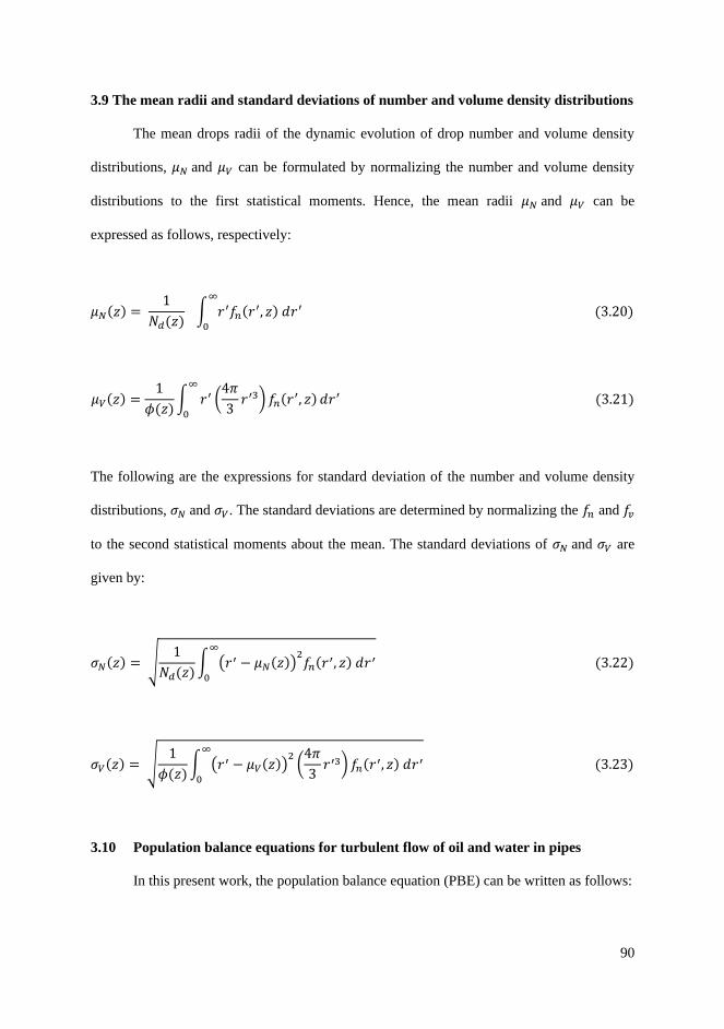
90
3.9 The mean radii and standard deviations of number and volume density distributions
The mean drops radii of the dynamic evolution of drop number and volume density
distributions, 𝜇𝑁 and 𝜇𝑉 can be formulated by normalizing the number and volume density
distributions to the first statistical moments. Hence, the mean radii 𝜇𝑁 and 𝜇𝑉 can be
expressed as follows, respectively:
𝜇𝑁(𝑧) = 1
𝑁𝑑(𝑧) ∫ 𝑟′𝑓𝑛(𝑟′, 𝑧) 𝑑𝑟′
∞
0
(3.20)
𝜇𝑉(𝑧) =1
𝜙(𝑧)∫ 𝑟′ (
4𝜋
3𝑟′3) 𝑓𝑛(𝑟′, 𝑧)
∞
0
𝑑𝑟′ (3.21)
The following are the expressions for standard deviation of the number and volume density
distributions, 𝜎𝑁 and 𝜎𝑉. The standard deviations are determined by normalizing the 𝑓𝑛 and 𝑓𝑣
to the second statistical moments about the mean. The standard deviations of 𝜎𝑁 and 𝜎𝑉 are
given by:
𝜎𝑁(𝑧) = √1
𝑁𝑑(𝑧)∫ (𝑟′ − 𝜇𝑁(𝑧))
2𝑓𝑛(𝑟′, 𝑧) 𝑑𝑟′
∞
0
(3.22)
𝜎𝑉(𝑧) = √1
𝜙(𝑧)∫ (𝑟′ − 𝜇𝑉(𝑧))
2(4𝜋
3𝑟′3) 𝑓𝑛(𝑟′, 𝑧) 𝑑𝑟′
∞
0
(3.23)
3.10 Population balance equations for turbulent flow of oil and water in pipes
In this present work, the population balance equation (PBE) can be written as follows:

91
𝑈𝜕𝑓𝑛(𝑟, 𝑧)
𝜕𝑧= ∫ 𝑟𝑐(𝑟
′, 𝑟′′)𝑓𝑛(𝑟′, 𝑧)𝑓𝑛(𝑟′′, 𝑧)𝑟2
𝑟′′2𝑑𝑟′
𝑟 √23⁄
0
− 𝑓𝑛(𝑟, 𝑧)∫ 𝑟𝑐(𝑟, 𝑟′)𝑓𝑛(𝑟′, 𝑧)
∞
0
𝑑𝑟′
+∫ 2𝛽(𝑟, 𝑟′)𝑔(𝑟′)𝑓𝑛(𝑟′, 𝑧)∞
𝑟
𝑑𝑟′ − 𝑔(𝑟)𝑓𝑛(𝑟, 𝑧) (3.24)
The population balance equations above are defined in the following domains:
0 ≤ 𝑧 ≤ 𝐿 , 0 ≤ 𝑟 ≤ ∞
In Eq. (3.24) above, 𝑓𝑛(𝑟, 𝑧) denotes the number density function in terms of 𝑟, radius of the
droplets (internal coordinate) and 𝑧, the axial position of the droplet in the pipe (external
coordinate).
In this present work, the PBE in Eqn. (3.24) is formulated in terms of number density
distribution, 𝑓𝑛(𝑟, 𝑧). From the fact that the magnitude of number density distribution 𝑓𝑛(𝑟, 𝑧)
can alter significantly during drop growth process, thus, the PBE in Eqn. (3.24) is modified to
account for volume density distribution, 𝑓𝑣(𝑟, 𝑧) in order to have a consistent magnitude over
time. One of the advantages of this approach is that the convergence criterion in terms of
relative tolerance and absolute tolerance are consistent with volume density distribution for
the numerical calculations. To achieve this, the volume fraction, 𝜙𝑣(𝑧) at a particular position
of 𝑧 coordinate is required. By applying the Eqn. (3.3) into Eqn. (3.24), the modified
population balance equation in terms of volume density distribution is given as follows:
𝑈𝜕𝑓𝑣(𝑟, 𝑧)
𝜕𝑧= 𝑣 ∫ 𝑟𝑐(𝑟
′, 𝑟′′)𝑓𝑣(𝑟
′, 𝑧)
𝑣′
𝑓𝑣(𝑟′′, 𝑧)
𝑣′′
𝑟2
𝑟′′2𝑑𝑟′
𝑟 √23⁄
0
− 𝑓𝑣(r, z)∫ 𝑟𝑐(𝑟, 𝑟′)
𝑓𝑣(𝑟′, 𝑧)
𝑣′
∞
0
𝑑𝑟′
+ 𝑣 ∫ 2𝛽(𝑟, 𝑟′)𝑔(𝑟′)𝑓𝑣(𝑟
′, 𝑧)
𝑣′
∞
𝑟
𝑑𝑟′ − 𝑔(𝑟)𝑓𝑣(𝑟, 𝑧) (3.25)
For 0 ≤ 𝑧 ≤ 𝐿 , 0 ≤ 𝑟 ≤ ∞

92
This new formulation (Eqn. 3.25) represents population balance equation in terms of volume
density distribution for dynamic evolution of droplet size in oil-water (turbulent) pipe flow.
This formulation describes the volume change per unit pipe length instead of number change
per unit pipe length. Thus, one could easily identify the coalescence birth relative to death at
larger droplet sizes. To simulate the model and facilitate the numerical solutions, the system
equations should be scaled into dimensionless variables. In this respect, the model is able to
characterize the system behaviour at dynamically similar system and different scales. The
scaling and the dimensionless analysis of the model equations are described in detail in the
Appendix A of this thesis. For comprehensive descriptions of the dimensionless techniques
and analysis, please refer to Part I of the manuscript – Appendix B.
3.11 Algorithm and numerical protocols
Following the non-dimensional conversions, the model equations are then solved
numerically starting from the initial distribution of the system. In this work, the algorithm is
written to operate on either a user defined distribution or from experimental data. In either
case, the values of the distribution might be arbitrary meaning it would not satisfy Eqn. (3.2).
To achieve this, the following methods are used:
The variables in the distribution are defined as follows:
𝑓𝑛0 ≈ 𝑓𝑛,𝑒𝑥𝑝,𝑖 𝑤ℎ𝑒𝑟𝑒 𝑖 = 1,2, …… .𝑁𝑖𝑛𝑖 (3.26)
𝑟𝑒 ≈ 𝑟𝑒𝑥𝑝,𝑖 𝑤ℎ𝑒𝑟𝑒 𝑖 = 1,2, …… .𝑁𝑖𝑛𝑖 (3.27)
𝛿𝑣 ≈4
3𝜋𝑟𝑒𝑥𝑝,𝑖
3 𝑤ℎ𝑒𝑟𝑒 𝑖 = 1,2, …… .𝑁𝑖𝑛𝑖 (3.28)

93
In the above equations from (3.26) until (3.28), 𝑟𝑒𝑥𝑝 represents the experimental droplet
radius, 𝑁𝑖𝑛𝑖 denotes the number of data (experimental data), and 𝛿𝑣 is the volume size of each
droplet in the distribution. Depending on the type of initial distributions (i.e., number density
distribution or volume density distributions), the integrations are approximated as follows:
The program reads in and integrates an arbitrary number density distribution:
𝐼𝑛 = ∫ 𝛿𝑣𝑓𝑛0𝑑𝑟′𝑟𝑒
0
= ∑(𝛿𝑣,𝑖𝑓𝑛,𝑒𝑥𝑝,𝑖
𝑁𝑖𝑛𝑖
𝑖=2
+ 𝛿𝑣,𝑖−1𝑓𝑛,𝑒𝑥𝑝,𝑖−1)(𝑟𝑒𝑥𝑝,𝑖 − 𝑟𝑒𝑥𝑝,𝑖−1)/2 (3.29)
The program reads in and integrates an arbitrary volume density distribution:
𝐼𝑣 = ∫ 𝑓𝑛0𝑒𝑑𝑟′
𝑟𝑒
0
= ∑(𝑓𝑛,𝑒𝑥𝑝,𝑖
𝑁𝑖𝑛𝑖
𝑖=2
+ 𝑓𝑛,𝑒𝑥𝑝,𝑖−1)(𝑟𝑒𝑥𝑝,𝑖 − 𝑟𝑒𝑥𝑝,𝑖−1)/2 (3.30)
Once the integration is determined, the number and volume density distributions can be
scaled as follows:
(i) For number basis
𝑓𝑛 =𝜙
𝐼𝑛𝑓𝑛0,𝑒𝑥𝑝 (3.31)
𝑓𝑣 = 𝑓𝑛𝛿𝑣 (3.32)
(ii) For volume basis
𝑓𝑣 =𝜙
𝐼𝑣𝑓𝑛0,𝑒𝑥𝑝 (3.33)
𝑓𝑛 = 𝑓𝑣/𝛿𝑣 (3.34)
It is worth noting that, the experimental data from FBRM technique supplied in this present
work are measured in terms of number density distribution, 𝑓𝑛. Hence, Eqns. (3.29), (3.31),
and (3.32) are employed for the experimental data used.

94
On the other hand, the parameter 𝑅𝑚𝑎𝑥 or maximum drop radius is introduced to the
system. The value of 𝑅𝑚𝑎𝑥 is set arbitrarily due to the fact that the exact value for 𝑅𝑚𝑎𝑥 is
unknown until the simulation is performed. In this respect, the value of 𝑅𝑚𝑎𝑥 is set large
enough such that the volume and number density distributions are not exceeding the 𝑅𝑚𝑎𝑥 as
they evolve. In addition, 𝑅𝑚𝑎𝑥 is important to the non-dimensionalization of the system
equations because it represents the characteristic length of the radial coordinate (internal
coordinate) in the scaling formulation (refer to Appendix A of dimensional analysis). Apart
from that, to facilitate interpolation of the experimental data and the simulation grid, an
arbitrary number of additional points are added between maximum experimental radius,
𝑅𝑚𝑎𝑥,𝑒𝑥𝑝 and 𝑅𝑚𝑎𝑥. The additional points are added if the condition of 𝑅𝑚𝑎𝑥 > 𝑅𝑚𝑎𝑥,𝑒𝑥𝑝 is
met.
3.11.1 Numerical protocol in non-dimensionalization system
On top of that, to enhance the numerical solutions, spectral elements (𝑛) are
introduced to the system. This is achieved by splitting the drop radius coordinate into several
domains, while the element boundaries are determined by 𝑟𝑛,𝑚𝑖𝑛 , 𝑟𝑛,𝑚𝑒𝑎𝑛, 𝑟𝑣,𝑎𝑡 𝑣𝑜𝑙𝑢𝑚𝑒 99%,
𝑟𝑣,log 𝑠𝑝𝑎𝑐𝑒 (from the logarithmic spacing), and 𝑟𝑚𝑎𝑥 (equivalent to 𝑅𝑚𝑎𝑥 in dimensional
system) of the volume density distribution as shown in Fig. 3.3 with 𝑓�̅� indicates the
dimensionless volume density distribution (refer to dimensionless analysis in Appendix A).
In this respect, the element end points or the boundaries in terms of dimensionless radius (𝜉𝑛)
can be determined as follows:
𝜉1 = 0/𝑅𝑚𝑎𝑥 = 0 (3.35)
𝜉2 = 𝑟𝑛,𝑚𝑖𝑛 𝑅𝑚𝑎𝑥⁄ (3.36)
𝜉3 = 𝑟 𝑛,𝑚𝑒𝑎𝑛 𝑅𝑚𝑎𝑥⁄ (3.37)

95
𝜉4 = 𝑟𝑣,𝑎𝑡 𝑣𝑜𝑙𝑢𝑚𝑒 99% 𝑅𝑚𝑎𝑥⁄ (3.38)
𝜉5 = 𝑟𝑣,log 𝑠𝑝𝑎𝑐𝑒 𝑅𝑚𝑎𝑥⁄ (3.39)
𝜉6 = 𝑟𝑚𝑎𝑥 𝑅𝑚𝑎𝑥⁄ = 1 (3.40)
Figure 3.3 schematic diagram of the radial coordinate and the properties of the volume
density distribution in terms of minimum radius, peak radius, mean radius, radius at 99%
volume, maximum experimental radius, and maximum (simulation) radius.
The total number of spectral elements, 𝑁𝑡 employed in the system is important in order to set
the element end point, 𝜉𝑛 for the system. For instance, if the total number of elements, 𝑁𝑡 ≥
5, the element end point, 𝜉𝑛 takes in the following value:
𝑁𝑡 ≥ 5, 𝜉𝑛 = 𝜉0, 𝜉𝑛,𝑚𝑖𝑛 , 𝜉𝑛,𝑚𝑒𝑎𝑛 , 𝜉𝑣,99, 𝜉𝑣,log 𝑠𝑝𝑎𝑐𝑒 , 𝜉1
96
In the expression above, 𝜉0 indicates the initial radius at zero coordinate, 𝜉𝑛,𝑚𝑖𝑛 represents
the smallest radius where the number density distribution is non zero, 𝜉𝑛,𝑚𝑒𝑎𝑛 denotes the
mean value of the number density distribution, 𝜉𝑣,99 signifies the radius located where the
volume density distribution integral (i.e., 𝜙) is 99% of the total integral value, and at the last
number of element (i.e., 𝑁𝑡 ≥ 5) the radius will be located at the logarithmically spaced
points between 𝜉𝑣,99 and 1.0 (i.e., 100) which refers to 𝜉𝑣,log 𝑠𝑝𝑎𝑐𝑒. Otherwise, (i.e., if 𝑁𝑡 < 5),
the element end point, 𝜉𝑛 will take the following steps:
𝑁𝑡 = 4, 𝜉𝑛 = 𝜉0, 𝜉𝑛,𝑚𝑖𝑛 , 𝜉𝑛,𝑚𝑒𝑎𝑛 , 𝜉𝑣,99, 𝜉1
𝑁𝑡 = 3, 𝜉𝑛 = 𝜉0, 𝜉𝑛,𝑚𝑒𝑎𝑛 , 𝜉𝑣,99, 𝜉1
𝑁𝑡 = 2, 𝜉𝑛 = 𝜉0, 𝜉𝑣,99, 𝜉1
𝑁𝑡 = 1, 𝜉𝑛 = 𝜉0, 𝜉1
Gauss-Lobatto Quadrature with Jacobi Polynomials is constructed for each of the
element (𝑛) along with user defined value for the number of internal collocation points in
each element, 𝑁𝑖𝑝𝑛 . In the numerical solutions, the degree of the Jacobi polynomials (𝑖) in
every element of 𝑁𝑖𝑝𝑛 can be varied. This method is essentially to provide numerical flexibility
in the lower values of the 𝑟 domain. In this regard, the dynamics for small drop coalescence
is very fast, hence, more points are needed to accommodate small 𝑟 values to provide
numerical accuracy and speed in the initial stages of the simulation. The advantage of this
feature in numerical scheme is that it allows one to place the collocation points strategically
in the spectral element and as a result the computational time can be reduced effectively.
Based on the value of 𝑁𝑖𝑝𝑛 for each element, a set of roots 𝑢𝑖
𝑛 and weights 𝑤𝑖𝑛 are calculated.
The roots are determined by Newton’s method from the shifted Jacobi polynomial on the

97
interval [0 1]. The integration weights, 𝑤𝑖𝑛 for each collocation point in the spectral elements
are calculated using Gauss-Lobatto Quadrature from the roots of the Jacobi polynomials and
its derivatives. The roots and weights calculated are used to approximate the integrals in the
system equations. The overall properties of the gridding system and layout of the elements
are depicted in Fig. 3. 4.
Figure 3.4 Schematic diagram of the gridding system and the overall layout of elements.
From the expression in Eqn. (3.42), the integration of volume density distribution and the
first derivative weight of volume density distribution can be written as follows, respectively:
∫ 𝑓�̅�𝑑𝜉1
0
= ∑ ∑ 𝑓�̅�,𝑗𝑛
𝑁𝑖𝑝𝑛 +2
𝑗=1
𝑁𝑡
𝑛=1
𝑙𝑛𝑤𝑗𝑛 (3.43)

98
𝑑𝑓�̅�,𝑖𝑛
𝑑𝜉|𝑢𝑖
𝑛
= ∑ ∑𝐴𝑖,𝑗
𝑛
𝑙𝑛𝑓�̅�,𝑗
𝑛
𝑁𝑖𝑝𝑛 +2
𝑗=1
𝑁𝑡
𝑛=1
(3.44)
In the algorithm, the matrices containing the first and second orders derivatives weights are
calculated from the roots of the Jacobi polynomial at each of the collocation point (𝑖). The
initial distributions can be interpolated onto the simulation grid once the simulation grid is
constructed. The interpolation technique by Akima spline interpolation is selected due to its
ability to produce smooth curves as well as its less proneness to wiggling (Salomon, 2011).
To solve the system equation, the integration limits in the birth integral must be in the range
of [0 1] and correspond to the orthogonal collocation weights constructed. Hence, the limits
of the integrals have to be transformed and the number and volume density distributions will
be then interpolated onto this new domain (coordinate system). To achieve this, the
dimensionless volume and number density distributions (i.e., 𝑓�̅� and 𝑓�̅�) are split into several
sections in the spectral elements as shown in Fig. 3.5. The algorithm used cubic spline
interpolation method due to the flexibility and suitability in the system to interpolate the birth
integrals at every time step onto this new domain (i.e., 𝑓�̅�𝑝 and 𝑓�̅�𝑝
). One of the attributes of
this numerical scheme is that it enables the raw experimental data for an initial droplet size
distribution to be employed. In addition, one feature of the spectral element method (𝑛)
introduced in the numerical scheme is it allows one to place the number of collocation points
(𝑖) in the system, strategically (details are discussed in Chapter 4 of this thesis). This feature
will enable the model to solve the system equation at much lesser time without compromising
the numerical stability and solutions.

99
Figure 3.5 The schematic diagram of the interpolated number density distribution, 𝑓�̅�𝑝 onto
coordinate system of 𝛼ˊand 𝛼ˊˊfor the coalescence birth integral.
For the case of coalescence birth integral (Eqn. 3.25), new integration coordinate 𝛼ˊ(𝜉) is
defined for every value of non-dimensional radius, 𝜉 in the domain. Based on the upper limit
in the coalescence birth integral, 𝜉 √23
⁄ , hence 𝛼ˊ can be formulated as follows:
𝛼ˊ =𝜉ˊ
𝜉
√23⁄
(3.45)
Based on the expression in Eqn. (3.45) above, the dimensionless radius 𝜉ˊand its derivative
𝑑𝜉ˊwith respect to 𝛼ˊ can be expressed as follows, respectively:

100
𝜉ˊ = (𝜉
√23 ) 𝛼ˊ (3.46)
𝑑𝜉ˊ = (𝜉
√23 ) 𝑑𝛼ˊ (3.47)
Subsequently, by taking into account the relationship of 𝜉ˊˊ = (𝜉3 − 𝜉ˊ3)1 3⁄
from the volume
conservation in the coalescence process and Eqn. (3.46), the following expression for 𝛼ˊˊ can
be obtained:
𝛼ˊˊ = (2 − 𝛼ˊ3)1 3⁄
(3.48)
The following are the expression for the coalescence birth and death processes in terms of
discretization.
Discretized forms of birth and death rates due to coalescence, respectively:
𝑃𝐶𝑏[𝜉𝑖, 𝜆] = 𝜉𝑖
3 (𝜉𝑖
√23 ) ∑ ∑
𝜉𝑖2
𝜉𝑗ˊˊ2
�̅�𝑐 (𝜉𝑗ˊ , [𝜉𝑖
3 − 𝜉𝑗ˊ3]
1 3⁄ )
𝑁𝑖𝑝𝑛 +2
𝑗=2
𝑁𝑡
𝑛=1
𝑓̅𝑣𝑝
′ ,𝑗𝑛 𝑓̅
𝑣𝑝′′,𝑗𝑛 𝑙𝑛𝑤𝑗
𝑛 (3.49)
𝑃𝐶𝑑(𝜉𝑖, 𝜆) = 𝑓�̅�,𝑗
𝑛 ∑ ∑ �̅�𝑐
𝑁𝑖𝑝𝑛 +2
𝑗=2
(𝜉𝑖, 𝜉𝑗)𝑓�̅�,𝑗
𝑛
�̅�𝑗𝑛 𝑙𝑛𝑤𝑗
𝑛
𝑁𝑡
𝑛=1
(3.50)
In Eqn. (3.49) above 𝑓�̅�𝑝 represents the interpolated dimensionless volume density
distribution. The equations are simulated for every collocation point across all spectral
elements.

101
On the other hand, for the breakage case, similar principles are applied in which the
limits for the breakage birth integral have to be scaled to range from 0 to 1. To achieve this,
the cubic spline interpolation method is employed to interpolate the distribution onto the new
coordinate grid as shown in Fig. 3.6.
Figure 3.6 The schematic diagram of the interpolated number density distribution, 𝑓�̅�𝑝 onto
coordinate system of 𝛼𝑏 for the breakage birth integral.
Similar to the coalescence case, a new integration coordinate 𝛼𝑏(𝜉) is defined for every value
of non-dimensional radius, 𝜉 in the domain. In this context, 𝜉ˊ along with its derivative
𝑑𝜉ˊwith respect to 𝛼𝑏 can be expressed as follows, respectively:

102
𝜉ˊ = 𝜉 + (1 − 𝜉)𝛼𝑏 (3.51)
𝑑𝜉ˊ = (1 − 𝜉)𝑑𝛼𝑏 (3.52)
Hence, the discretized breakage birth and death can be written in the following form:
Discretized form of birth and death rates due to breakage, respectively:
𝑃𝐵𝑏[𝜉𝑖, 𝜆] = [1 − 𝜉𝑖]𝜉𝑖
3 ∑ ∑ 2�̅�
𝑁𝑖𝑝𝑛 +2
𝑗=1
(𝜉𝑖, 𝜉𝑗)�̅�(𝜉𝑗)𝑓�̅�𝑝,𝑗𝑛 𝑙𝑛𝑤𝑗
𝑛
𝑁𝑡
𝑛=1
(3.53)
𝑃𝐵𝑑(𝜉𝑖, 𝜆) = [�̅�(𝜉𝑖) 𝑓�̅�,𝑗
𝑛 ] (3.54)
Where in Eqn. (3.53), the expression of 𝜉𝑗 can be written as follows:
𝜉𝑗 = 𝜉𝑖 + (1 − 𝜉𝑖)𝛼𝑏,𝑗 (3.55)
Finally, the resulting ODE with initial conditions is numerically solved using Gear’s
backward differentiation formulae (BDF) method and integrated for over the 𝑧 coordinate.
3.12 Physical properties of the oil-water system
In this work, three different data sets supplied by Statoil were measured from the
Focused Beam Reflectance Method (FBRM) for the turbulently flowing oil-water system.
The data sets in this present work are classified as ge12275a, ge12279a, ge12284a. The
physical properties of each of the data set are shown in Table 3.1. It is worth to note that, the
major difference between the three data sets is the average flow velocity, 𝑈. As depicted in

103
Table 3.1, ge12284 represents the highest average flow velocity, 𝑈 at 2.50 m/s, followed by
ge12279a and ge12275a with 2.0 m/s and 1.70 m/s, respectively. These physical parameters
of the system are used as inputs for the model simulations.
Table 3.1 The physical properties of the oil-water system in pipe
Parameter Ge12275a Ge12279a Ge12284a Descriptions
𝜙 0.30 0.30 0.30 Volume fraction
𝑈 1.70 [m/s] 2.00 [m/s] 2.50 [m/s] Average flow velocity
𝐿 30 [m] 30 [m] 30 [m] Length of the pipe
𝑅𝑚𝑎𝑥 1000 [μm] 1000 [μm] 1000 [μm]
Upper bound of the radius
domain
𝐷 0.069 [m] 0.069 [m] 0.069 [m] Diameter of the pipe
𝜌𝑑 865 [kg/m3] 865 [kg/m3] 865 [kg/m3] Density of the dispersed phase
𝜇𝑑 177 [mPas] 169 [mPas] 152 [mPas] Viscosity of the dispersed phase
𝜌𝑐 1021 [kg/m3] 1021 [kg/m3] 1021 [kg/m3] Density of the continuous phase
𝜇𝑐 1.0 [mPas] 1.0 [mPas] 1.0 [mPas]
Viscosity of the continuous
phase
σ 26.0 [mN/m] 26.0 [mN/m] 26.0 [mN/m] Interfacial tension
3.13 Experimental data of droplet size distribution
When oil and water are transported through pipeline under vigorous shear rates, the
formation of dispersion between oil and water will occur. In laboratory work, one of the
techniques to record the droplet size distribution during dispersion process of oil and water in
dynamic pipe transportation is using Focused Beam Reflectance Measurement (FBRM). The
method of using FBRM probe has been studied in detail experimentally in horizontal pipes by

104
Placensia (2013) and Schümann (2016). Their research work suggested that FBRM probe can
provide in-situ drop size evolution measurement through oil-water pipe flow. In this research
work, the in-situ measurement of droplet size distribution profiles was obtained using two
FBRM probes, one at the inlet and the other one at the outlet of the pipe. The advantages of
using FBRM are droplet size variations in the dispersion process can be easily tracked
compared to other instrument such as Particle Video Microscope (PVM) and real time
measurement of particle size, count and shape can be obtained during oil-water emulsion in
turbulent pipe flow (Placensia, 2013). FBRM utilizes highly precise chord length distribution
(CLD), sensitive to particle size and count under real-time measurement without the need of
sample preparation. FBRM is capable to measure droplet size in the range of 0.8-1000 μm
which is ideal for in-situ droplet size analysis in real time (Dowding et al., 2001).
(a) (b)
Figure 3.7 FBRM Measurement (a) Schematic of FBRM probe tip (b) Particle size
distribution using FBRM probe (Worlitschek and Buhr, 2005).

105
In general, the droplet size distribution was measured during the experimental work
once the flow of oil-water dispersions reached a stabilized oil-water dispersion (steady state
condition: stable pressure drop, mixture density, temperature and droplet size). In addition,
the homogeneity of the mixture was also tracked by measuring the mixture density using the
Coriolis flow meter during the dynamic flow of oil-water dispersion. These conditions must
be met to ensure the quality of the droplet size distribution profiles obtained are accurate. It is
to be noted that the experimental data of droplet size distributions were completely supplied
by Statoil Research Centre, Trondheim. Hence, the validation of data was performed by the
appointed researcher from Statoil. The samples of experimental data of drop size distribution
is depicted in Fig. 3.8. FBRM probe is known to be one of the exceptional methods to
measure real time droplet size distribution in liquid-liquid system. This is indicated by
numerous studies on oil-water system using FBRM method (Maaß et al., 2011; Schümann et
al., 2015; Schümann, 2016; Plasencia, 2013; Boxall et al., 2010; Naeeni and Pakzad, 2019).
Figure 3.8 Samples of number density distributions for oil-water dispersions in pipe flow
using FBRM probe. The 𝑓𝑛,𝑒𝑥𝑝 indicates experimental number distribution and 𝑓𝑛,0 the
interpolated number distribution.

106
During the lab experiment of this current project, no other devices for droplet
monitoring installed in the flow loop (pipes). However, to ensure the quality of the data
obtained, direct comparison of drop size distribution profiles was established using PVM
simultaneously with FBRM probes in a separate experiment in stirred tank setup using the
same fluids. A conversion factor was derived from the comparison results of chord length
distribution (CLD) from FBRM to real droplet size and distribution. Thorough discussion on
the conversion factor can be found in research work by Khatibi, (2013) and Schümann et al.
(2015). In addition, Boxall et al. (2010) also suggested that PVM probe is a useful tool for a
calibration method with FBRM probe. For this present work, the shape of the droplet from
experimental data is assumed spherical. Therefore, the mean chord length size measured by
FBRM corresponds to the diameter of the droplet. However, there will be uncertainty in the
chord length measured by the FBRM from the real droplet size distribution due to several
factors such off-center crossing of the droplets by the laser beam, dense emulsions scattering
of light by other droplets, variation in refractive index of the liquids, surface structures and
properties such as translucent or transparent surface that may cause internal reflection and/or
subsurface scattering (Vay et al., 2012; Schümann et al., 2015). Therefore, a general
correction has been proposed by comparing simultaneous FBRM with PVM measurements in
the same fluid system in order to reduce underestimation of the droplet size. The method
allows combination of both techniques and produce real time and in situ measurement of
correct droplet sizes although with an uncertainty of 50% (Schümann et al., 2015). This
method introduced the log-normal distribution function to describe the droplet size
distribution and it can be written as follows (Farr, 2013):
𝑓(𝐷) =1
𝐷𝜎√2𝜋𝑒𝑥𝑝 {
[ln(𝐷 𝐷0⁄ )]2
2𝜎2} (3.56)

107
Where 𝑓(𝐷) is log-normal function of the droplet size distribution, 𝐷 is the droplet size, 𝜎 is
the dimensionless geometric standard deviation (the width of the distribution) and 𝐷0 is a
reference diameter setting the scale or the length scale of the distribution. According to
Schümann et al. (2015), the conversion method from FRBM measurements has successfully
reduced the error from factor of five to factor of two. Since the distribution of droplet size is
commonly presented in logarithmic scale, thus, the error is considered within the acceptable
limits. The conversion has been applied for this research work across all the measurements
and the particle sizes measured from the three different experiments are observed to be in the
range of 1.00 μm to 616.00 μm (refer to Table 3.2 and Fig. 3.8). It is worth to note that, the
author is not involved in the experimental work. Hence, details about the experimental
procedures and data preparations are exclusively owned by Statoil.
Table 3.2 Size range of the droplets from three different data sets of oil-water pipe flow
Experimental data set Size range of the droplets
Ge12275a 1.00 μm – 616.00 μm
Ge12279a 1.00 μm – 575.00 μm
Ge12287a 1.00 μm – 537.00 μm

108
Figure 3.9 Overview of the simulation flow processes
109
3.14 Chapter summary
In this chapter, all models derived and formulated are showed and elucidated in each
subsection. Since the system equations involve turbulent flows, assumptions have to be made
(in early subsections) in order to simplify and enhance the simulation work. In the model
formulation, possible methodologies are introduced using orthogonal collocation approach on
finite elements as an alternative technique to solve the PBE. For any axial position in
pipeline, the model developed from this method is able to predict the evolution of number
and volume density distributions, the average drop radii for number and volume density
distributions, the standard deviations of the droplet in terms of number and volume density
distributions, and the rates of breakage and coalescence as well as total growth rates over a
distance in pipes. For more comprehensive and details discussions of the model formulations
and techniques, the reader is encouraged to refer to Part I of this manuscript in the attachment
of Appendix B.

110
CHAPTER 4
4 RESULTS AND DISCUSSION (PART I)
4.1 Simulation results and discussion
In this thesis, the results and discussion are divided into two main parts: (i) the model
behaviour and parametric effects and (ii) regression of the experimental pipe flow data:
comparison between simulation and experimental data. The first part (Part I) is discussed in
this chapter – Chapter 4, while the second part (Part II) is discussed in the next chapter –
Chapter 5. In these two chapters (i.e., Chapter 4 and Chapter 5), two manuscripts are prepared
for each of the results discussed in Part I and Part II. Including the paper prepared in Chapter
3, there are three manuscripts altogether for this research work and they can be found in the
Appendix B, Appendix C, and Appendix D of this thesis, respectively.
4.2 Part I: The model behaviour and parametric effects
In liquid-liquid systems, many physical properties of the dispersion are strongly
related to the drop size distribution of the dispersed phase. In pipe flow, any changes in the
drop size distribution may affect the flow pattern and pressure drop significantly. Hence, the
evaluation and study of parametric effect is important because coalescence and breakage
processes in liquid-liquid turbulent pipe flow are strongly dependent on the physical
properties of the continuous and dispersed phase, state of flow, and mixing conditions in the
system (Solsvik et al., 2015). For this purpose, the model is investigated under various
parametric effects to provide insights toward the overall model behaviour. For these
investigations, the following physical properties as shown in Table 4.1 are employed as an
input for the simulation.

111
Table 4.1 Input parameters for the simulation
Parameter Value Descriptions
𝜙 0.30 Volume fraction
𝑈 2.00 [m/s] Average flow velocity
𝐿 1500 [m] Length of the pipe
𝑅𝑚𝑎𝑥 1000 [μm] Upper bound of the radius domain
𝐷 0.069 [m] Diameter of the pipe
𝜌𝑑 865 [kg/m3] Density of the dispersed phase
𝜇𝑑 169 [mPas] Viscosity of the dispersed phase
𝜌𝑐 1021 [kg/m3] Density of the continuous phase
𝜇𝑐 1.0 [mPas] Viscosity of the continuous phase
σ 26.0 [mN/m] Interfacial tension
Depicted in Fig. 4.1 is the plot of experimental number density distribution, 𝑓𝑛,𝑒𝑥𝑝 at initial
position in the pipe (𝑧 = 0) as a function of drop radius, 𝑟. The distribution is then compared
against the interpolated initial number density distribution, 𝑓𝑛,0. On the same figure, the
experimental and interpolated volume density distributions, 𝑓𝑣,𝑒𝑥𝑝 and 𝑓𝑣,0 respectively, are
also plotted against the drop radius, 𝑟. Essentially, the comparison between the experimental
and interpolated distributions is to map the experimental data points onto the collocation
points that consist of simulation grid. In this respect, the interpolation was showing good
results wherein the interpolated initial number and volume density distributions, 𝑓𝑛,0, 𝑓𝑣,0 are
perfectly fits with the experimental data points consistently.

112
Figure 4.1 Initial experimental number and volume density distributions, 𝑓𝑛,𝑒𝑥𝑝, 𝑓𝑣,𝑒𝑥𝑝 in blue
and red dotted lines, and interpolated initial number and volume distributions, 𝑓𝑛,0, 𝑓𝑣,0 in
blue and red circles, are plotted as a function of droplet radius, 𝑟.
4.2.1 Base case
In this present work, a base case is prepared as a reference to give an overview of how
the system behaves with the given set of input parameters. For this purpose, the following
fitting parameters are used as shown in Table 4.2.
Table 4.2 Base case: fitting parameters
Parameter Value Descriptions
𝑘𝜔 1.00 𝑒 -04 Fitting parameter for coalescence frequency expression
𝑘𝜓 1.00 𝑒 -03 Fitting parameter for coalescence efficiency expression
𝑘𝑔1 5.00 𝑒 -01 Fitting parameter for breakage frequency expression
𝑘𝑔2 5.00 𝑒 -01 Fitting parameter for breakage efficiency expression

113
From the set of fitting parameters above, the evolution of the number and volume
density distributions (𝑓𝑛 and 𝑓𝑣) are simulated and depicted in Fig. 4.2. From the figure, the
dynamic evolution of 𝑓𝑛 and 𝑓𝑣 of the base case are plotted in terms of radius, 𝑟, throughout
nine different axial (𝑧) locations in the pipeline. The number density distribution, 𝑓𝑛 in Fig.
4.2(a) demonstrates that there is a small quantity of larger size droplets at the beginning of
the pipeline and the magnitude of 𝑓𝑛 grows higher as the droplets evolve toward the end of
the pipeline. This is true considering that the larger droplets present at the beginning of the
pipeline are more likely to break than smaller droplets. This indicates that breakage is
dominant in the system at short axial distances. Similarly, for volume density distribution, 𝑓𝑣,
the magnitude increases towards the end of pipeline. This shows that, coalescence balances
breakage as axial (𝑧) increases and the distribution reaches equilibrium. An increasing
magnitude of drops evolution (𝑓𝑣) as shown in Fig. 4(b) suggests that, the distribution is
narrower at equilibrium relative to the initial condition, in which there are large numbers of
small droplets formed at the end of the pipeline.
(a)
(b)

114
Figure 4.2 Evolution of (a) number density distribution, 𝑓𝑛 and (b) volume density
distribution, 𝑓𝑣 along the pipeline as a function of drop radius, 𝑟. The fitting parameters used
are shown on top left corner of the plots for the base case.
On the other hand, Fig. 4.2 illustrates the dynamic evolution of mean radii in terms of
number and volume density distributions (𝜇𝑁 and 𝜇𝑉) as a function of axial position, 𝑧 of the
pipe for the base case. The mean radii in Fig. 4.3 depict that, 𝜇𝑁 and 𝜇𝑉 are decreasing as the
droplets travel through the 1500 m pipeline. This suggests that, breakage is initially dominant
over coalescence for this set of fitting parameters and initial distribution (i.e., base case) as
the droplets evolve towards the end of the pipeline. It is worth noting that the mean radii of
𝜇𝑁 and 𝜇𝑉 are equilibrated after they surpass the 1 m of pipeline. As this takes place, the
mean radii have reached constant values in which the system is in balance between the
breakage and coalescence processes particularly, at the equilibrium state. Similar events are
found to occur in the standard deviations for number and volume density distribution, 𝜎𝑁 and
𝜎𝑉, as shown in Fig. 4.3(b). The magnitudes for both 𝜎𝑁 and 𝜎𝑉 are gradually decreasing as
they approach the end of the pipeline. They are also found to be levelled once the system
reaches the equilibrium.
(a)

115
(b)
Figure 4.3 The plot of: (a) the average radii of number density distribution, 𝜇𝑁 and volume
density distribution, 𝜇𝑉 as a function of axial position, 𝑧 in the pipe, and (b) the standard
deviations of number density distribution, 𝜎𝑁 and volume density distribution, 𝜎𝑉 as a
function of axial position, 𝑧 in the pipe. The fitting parameters used are shown on top left
corner of the plot for the base case.
To further evaluate the drop growth from the PBE model, the total coalescence and
breakage rates, 𝑅𝐶𝑡 and 𝑅𝐵𝑡
are plotted as a function of drop radius 𝑟 for nine different
locations as shown in Fig. 4.4. In this figure, the positive part of the curve indicates the birth
and the negative part of the curve represents the death by virtue of coalescence and breakage
processes. In Fig. 4.4(a), the total coalescence rate is lower in magnitude at the beginning of
the pipeline and as axial position, 𝑧 increases, the rate gets higher. This suggests that,
coalescence rate is stronger approaching the end of the pipe and somewhat weaker at the
beginning stage in the pipe. This is true considering the large number of smaller droplets
presence towards the end of the pipe. Hence, coalescence is expected to increase towards the
end of the pipeline due to the fact that small droplets are more likely to coalesce, and the
larger number density promotes collision, while larger droplets tend to rupture. Conversely,
the total breakage rate, 𝑅𝐵𝑡 in Fig. 4.4(b) is found to reduce in magnitude as the breakage
process moves towards the end of the pipeline. Moreover, it is expected that 𝑅𝐵𝑡 is found to
be greater at low 𝑧 values because larger droplets at the onset of the pipeline are easier to

116
break and rupture than smaller droplets at the end. Apart from that, the birth rate due to
breakage shown in Fig. 4.4(b) is observed to be higher (i.e., 𝑅𝐵𝑡≈ 2000) than the death rate
by breakage (i.e., 𝑅𝐵𝑡≈ -1200). This is primarily because of the difference in the number of
larger droplets present at the beginning of the pipeline than at the end which will significantly
affect the breakage frequency and efficiency.
(a)
(b)
Figure 4.4 Evolution of (a) total coalescence rate, 𝑅𝐶𝑡and (b) total breakage death rate, 𝑅𝐵𝑡
.
Both rates are plotted for the base case parameter set and as a function of droplet radius, 𝑟 at
nine different locations from 1500 m pipe length. The fitting parameters used are shown on
top left corner of the plots for the base case.
4.2.2 Numerical techniques and model behavior
Prior to analysis on various parametric effects, the model performance is assessed in
terms of the proposed numerical technique (orthogonal collocation method) as described in
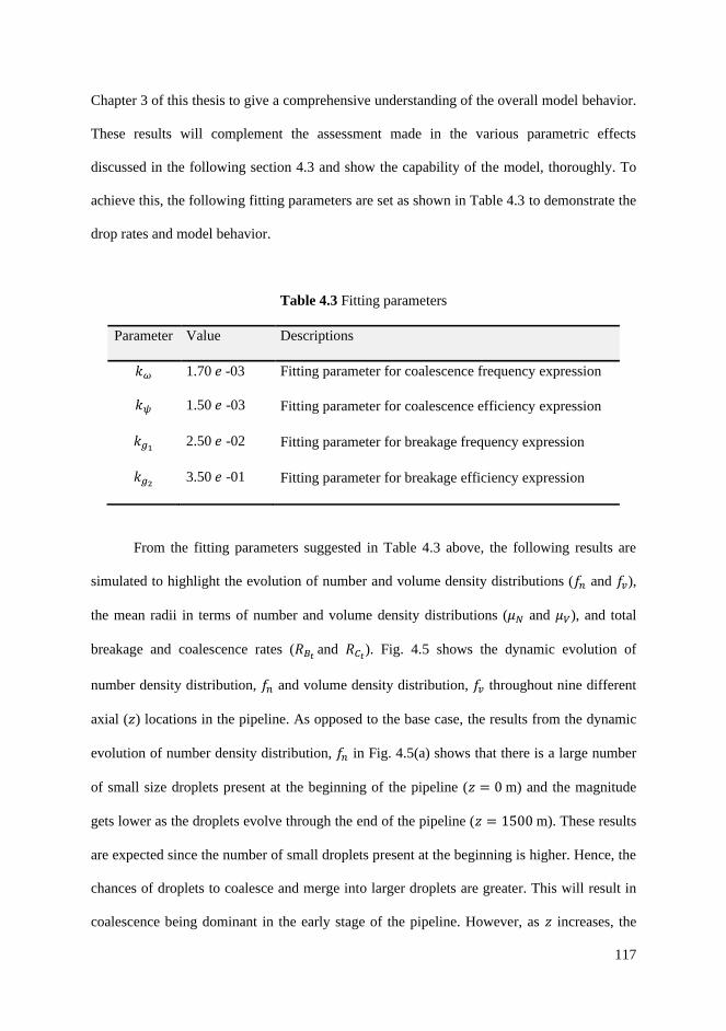
117
Chapter 3 of this thesis to give a comprehensive understanding of the overall model behavior.
These results will complement the assessment made in the various parametric effects
discussed in the following section 4.3 and show the capability of the model, thoroughly. To
achieve this, the following fitting parameters are set as shown in Table 4.3 to demonstrate the
drop rates and model behavior.
Table 4.3 Fitting parameters
Parameter Value Descriptions
𝑘𝜔 1.70 𝑒 -03 Fitting parameter for coalescence frequency expression
𝑘𝜓 1.50 𝑒 -03 Fitting parameter for coalescence efficiency expression
𝑘𝑔1 2.50 𝑒 -02 Fitting parameter for breakage frequency expression
𝑘𝑔2 3.50 𝑒 -01 Fitting parameter for breakage efficiency expression
From the fitting parameters suggested in Table 4.3 above, the following results are
simulated to highlight the evolution of number and volume density distributions (𝑓𝑛 and 𝑓𝑣),
the mean radii in terms of number and volume density distributions (𝜇𝑁 and 𝜇𝑉), and total
breakage and coalescence rates (𝑅𝐵𝑡 and 𝑅𝐶𝑡). Fig. 4.5 shows the dynamic evolution of
number density distribution, 𝑓𝑛 and volume density distribution, 𝑓𝑣 throughout nine different
axial (𝑧) locations in the pipeline. As opposed to the base case, the results from the dynamic
evolution of number density distribution, 𝑓𝑛 in Fig. 4.5(a) shows that there is a large number
of small size droplets present at the beginning of the pipeline (𝑧 = 0 m) and the magnitude
gets lower as the droplets evolve through the end of the pipeline (𝑧 = 1500 m). These results
are expected since the number of small droplets present at the beginning is higher. Hence, the
chances of droplets to coalesce and merge into larger droplets are greater. This will result in
coalescence being dominant in the early stage of the pipeline. However, as 𝑧 increases, the
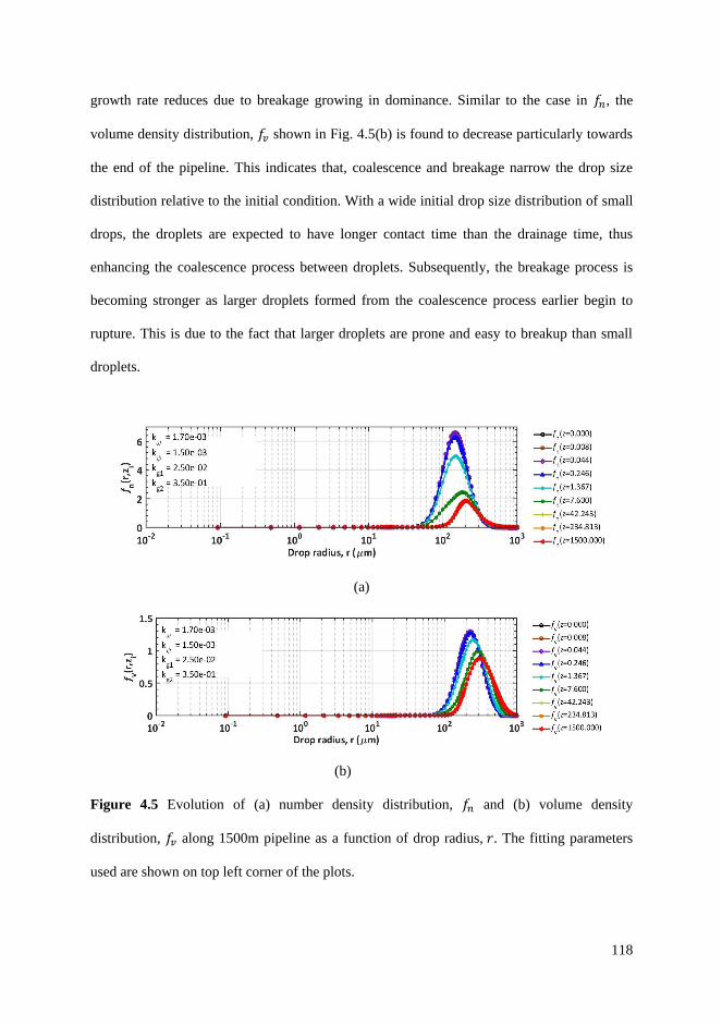
118
growth rate reduces due to breakage growing in dominance. Similar to the case in 𝑓𝑛, the
volume density distribution, 𝑓𝑣 shown in Fig. 4.5(b) is found to decrease particularly towards
the end of the pipeline. This indicates that, coalescence and breakage narrow the drop size
distribution relative to the initial condition. With a wide initial drop size distribution of small
drops, the droplets are expected to have longer contact time than the drainage time, thus
enhancing the coalescence process between droplets. Subsequently, the breakage process is
becoming stronger as larger droplets formed from the coalescence process earlier begin to
rupture. This is due to the fact that larger droplets are prone and easy to breakup than small
droplets.
(a)
(b)
Figure 4.5 Evolution of (a) number density distribution, 𝑓𝑛 and (b) volume density
distribution, 𝑓𝑣 along 1500m pipeline as a function of drop radius, 𝑟. The fitting parameters
used are shown on top left corner of the plots.
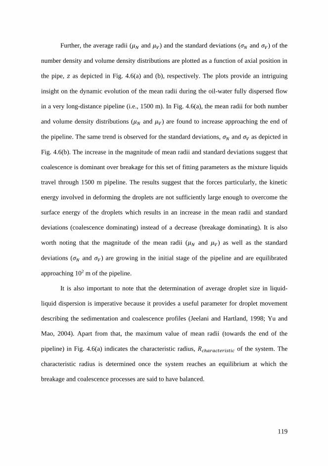
119
Further, the average radii (𝜇𝑁 and 𝜇𝑉) and the standard deviations (𝜎𝑁 and 𝜎𝑉) of the
number density and volume density distributions are plotted as a function of axial position in
the pipe, 𝑧 as depicted in Fig. 4.6(a) and (b), respectively. The plots provide an intriguing
insight on the dynamic evolution of the mean radii during the oil-water fully dispersed flow
in a very long-distance pipeline (i.e., 1500 m). In Fig. 4.6(a), the mean radii for both number
and volume density distributions (𝜇𝑁 and 𝜇𝑉) are found to increase approaching the end of
the pipeline. The same trend is observed for the standard deviations, 𝜎𝑁 and 𝜎𝑉 as depicted in
Fig. 4.6(b). The increase in the magnitude of mean radii and standard deviations suggest that
coalescence is dominant over breakage for this set of fitting parameters as the mixture liquids
travel through 1500 m pipeline. The results suggest that the forces particularly, the kinetic
energy involved in deforming the droplets are not sufficiently large enough to overcome the
surface energy of the droplets which results in an increase in the mean radii and standard
deviations (coalescence dominating) instead of a decrease (breakage dominating). It is also
worth noting that the magnitude of the mean radii (𝜇𝑁 and 𝜇𝑉) as well as the standard
deviations (𝜎𝑁 and 𝜎𝑉) are growing in the initial stage of the pipeline and are equilibrated
approaching 102 m of the pipeline.
It is also important to note that the determination of average droplet size in liquid-
liquid dispersion is imperative because it provides a useful parameter for droplet movement
describing the sedimentation and coalescence profiles (Jeelani and Hartland, 1998; Yu and
Mao, 2004). Apart from that, the maximum value of mean radii (towards the end of the
pipeline) in Fig. 4.6(a) indicates the characteristic radius, 𝑅𝑐ℎ𝑎𝑟𝑎𝑐𝑡𝑒𝑟𝑖𝑠𝑡𝑖𝑐 of the system. The
characteristic radius is determined once the system reaches an equilibrium at which the
breakage and coalescence processes are said to have balanced.
120
(a)
(b)
Figure 4.6 The plot of: (a) mean radii of number density distribution, 𝜇𝑁 and volume density
distribution, 𝜇𝑉 as a function of axial position, 𝑧 in the pipe and (b) standard deviations of
number density distribution, 𝜎𝑁 and volume density distribution, 𝜎𝑉 as a function of axial
position, 𝑧 in the pipe. The fitting parameters used are shown on top left corner.
4.2.2.1 The importance of conversion from 𝒇𝒏 to 𝒇𝒗
It is important to note that, in this work, the solutions of PBE are solved in terms of
the volume density distribution, 𝑓𝑣 instead of number density distribution, 𝑓𝑛. This can be
done by converting the system equation as depicted in Eqn. 3.25 of Chapter 3. To elucidate
the importance of volume density distribution, 𝑓𝑣 in solving the PBE, we employed two
different initial distributions in the system. The primary reason is to compare the evolution of
total number density function, �̅�𝑑 and volume fraction, 𝜙 across 1500m pipeline as shown in
Fig. 4.7. In this comparison, the three different initial distributions are named as case I, case
II, and case III. The main difference between the initial distributions in case I, case II, and

121
case III is the average flow velocity, 𝑈 in the pipes. The average flow velocity of the liquid-
liquid system in the pipes increases from case I to case III. Fig. 4.7 demonstrates the
comparison between the total number density function, �̅�𝑑 and the volume fraction, 𝜙 in
terms of axial position, 𝑧 in the pipeline for all the cases employed (i.e., cases I, II, and III).
The results in Fig. 4.7(a) show that, at increase number of cases (i.e., cases I, II, III), the total
number density as a function of axial position, 𝑁𝑑(𝑧) decreases in terms of the magnitude
towards the end of the pipeline. While, the results of volume fraction, 𝜙 for all the cases
simulated remain constant throughout the pipeline as depicted in Fig. 4.7(b). This clearly
shows that, the magnitude of number density distribution 𝑓𝑛 can alter significantly during the
drop growth compared to the magnitude of volume density distribution, 𝑓𝑣. In this respect,
one can have an insight that solving the PBE for dynamic evolution of drop size density
distribution in liquid-liquid system over a distance in pipe is more effective in the form of
volume density distribution, 𝑓𝑣 instead of number density distribution, 𝑓𝑛 (which has been
widely used in the literature) due to its consistent magnitude over time. This is primarily
crucial in order to ensure that the convergence criteria for the absolute and relative error
tolerances of the numerical integrator are consistent with the magnitude of the dependent
variable over the entire simulation.
(a)

122
(b)
Figure 4.7 The evolution of (a) dimensionless total number density function, �̅�𝑑 as a function
of axial position, 𝑧 and (b) the volume fraction of droplets, 𝜙 as a function of axial position,
𝑧. Both are plots in terms of case I, case II and case III of different initial distributions. The
fitting parameters used are shown on top left corner of the plots.
4.2.2.2 Error analysis on the numerical methods
In this present work, the error from the mass balance (𝜙) and the volume density
distribution, 𝑓𝑣 at equilibrium are assessed to give an overview of the overall system
behaviour. To achieve this, four cases are prepared with different model behaviors: case I
(coalescence-dominated), case II (breakage-dominated), case III (fast dynamics), and case IV
(slow dynamics). Each of the cases is set with different fitting parameters to elucidate the
model behavior in which, case I employs higher magnitude of and 𝑘𝑔1 and 𝑘𝑔2
(higher mean
radii), case II employs lower magnitude of 𝑘𝑔1 and 𝑘𝑔2
(lower mean radii), case III employs
greater magnitude of 𝑘𝜔 and 𝑘𝑔1(faster equilibrium), and case IV employs smaller magnitude
of 𝑘𝜔 and 𝑘𝑔1(slower equilibrium). Fig. 4.8 (a), (b), (c), and (d) indicate the mass balance
error analysis for case I, II, III, and IV at different total number of spectral elements, 𝑁𝑡 and
total number of points, 𝑖𝑡𝑜𝑡. In general, the error is greater as lower number of points are
allocated and conversely for higher number of points, regardless of the total number of
spectral elements employed (𝑁𝑡 = 1 or 𝑁𝑡 = 6). However, the error is found to be
significantly lower when total number of spectral elements, 𝑁𝑡 = 6 is used instead of 𝑁𝑡 =

123
1. Increment in the number of total collocation points, 𝑖𝑡𝑜𝑡 particularly, at 𝑁𝑡 = 6 has
effectively decreased the magnitude of the mass balance error. This indicates that, spectral
element method of 𝑁𝑡 = 6 is more efficient in numerical solutions for all types of cases (i.e.,
coalescence and breakage dominated systems and slow and fast dynamics systems) due to the
strategic placement of collocation points in the system. Ideally, increase in number of points
provides efficient numerical solutions (lower mass balance error) as sufficient number of
points are places to accommodate the droplets evolution over the axial position, 𝑧, but at the
cost of longer simulation times.
(a)
(b)

124
(c)
(d)
Figure 4.8 The mass balance error: (a) case I – coalescence dominated, (b) case II – breakage
dominated, (c) case III – fast dynamics, and (d) case IV – slow dynamics.
On the other hand, the volume density distribution (𝑓𝑣) at equilibrium with different
total number of spectral elements (𝑁𝑡) and collocation points (𝑖𝑡𝑜𝑡) employed are
demonstrated in Fig. 4.9 (a), (b), (c), and (d) for all cases (coalescence-dominated, breakage-
dominated, fast dynamics, and slow dynamics), respectively. The volume density distribution
(𝑓𝑣) in Fig. 4.9 shows that the distributions at equilibrium are varied for all cases in terms of
different spectral elements methods (i.e., 𝑁𝑡 = 1 and 𝑁𝑡 = 6) and collocation points. The

125
magnitude of 𝑓𝑣 is found to be maximum when higher number of collocation points are
allocated for both spectral element methods (𝑁𝑡 = 1 and 𝑁𝑡 = 6) in all cases. On the
contrary, if a smaller number of points are employed, the magnitude of 𝑓𝑣 reduces due to the
losses in mass balance, particularly in case III of fast dynamics system as shown Fig. 4.9(c).
In fast dynamics system, the event of small drop coalescence and large drop breakup
especially at equilibrium occurs at a faster rate. Hence, more points are required in order to
accommodate the stiffness of the numerical system in the 𝑟 domain. In this respect, enhanced
numerical accuracy can be expected. Furthermore, the results of 𝑓𝑣 complement with the error
results obtained in the mass balance errors depicted Fig. 4.8. In this error analysis of the
system from case to case basis, both methods 𝑁𝑡 = 1 and 𝑁𝑡 = 6 are found to reduce the
errors in the numerical system as higher number of collocation points are set. However, the
spectral element method ( 𝑁𝑡 = 6) is considered the best method to be employed in the
model due to the performance of spectral element methods 𝑁𝑡 = 6 is much better and
efficient than single element method 𝑁𝑡 = 1. The spectral element methods, 𝑁𝑡 = 6 produced
the lowest error than one element method ( 𝑁𝑡 = 1) irrespective of the total number of points
(𝑖𝑡𝑜𝑡) employed. In orthogonal collocation method, for each of the spectral element assigned,
one can strategically place the number of points to specifically account for the stiffness in the
numerical system. For instance, if the dynamics for small drop coalescence is very fast
particularly at lower 𝑟 domain, hence, more points can be strategically placed in this domain
to accommodate these small 𝑟 values (due to fast coalescence process) instead of uniformly
distributed (placement) collocation points as shows in the single element method (𝑁𝑡 = 1). In
this respect, the numerical accuracy and speed (refer to Table 4.4) can be enhanced due to
strategic distribution of collocation points in the system.
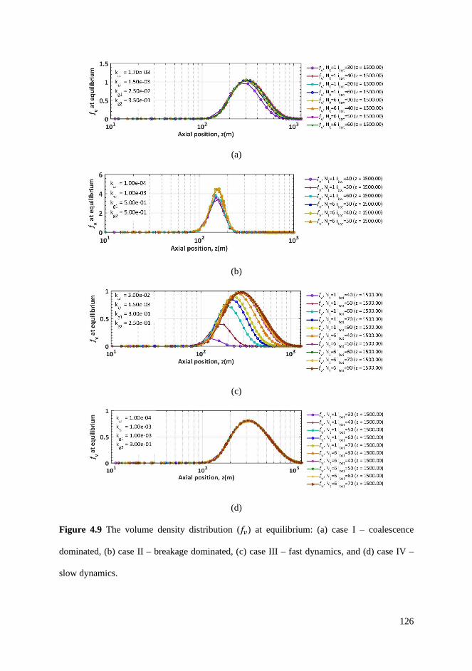
126
(a)
(b)
(c)
(d)
Figure 4.9 The volume density distribution (𝑓𝑣) at equilibrium: (a) case I – coalescence
dominated, (b) case II – breakage dominated, (c) case III – fast dynamics, and (d) case IV –
slow dynamics.

127
Apart from that, CPU time and simulation time for all the cases studied (i.e., case I, II,
III, and IV) at 𝑁𝑡 = 6 and 𝑁𝑡 = 1 are also investigated as depicted in Table 2. The results
suggest that, a system with spectral elements (i.e., sub-domain of 𝑁𝑡 = 6) provide lower
CPU time and faster simulation time. This is true considering the fact that, strategic numbers
of collocation points placed at different spectral elements promote faster numerical
convergence. In other words, one may choose 𝑁𝑡 = 1 and higher number 𝑖𝑡𝑜𝑡 but at cost of
CPU expensive and longer simulation time. However, with the spectral element scheme, low
CPU time and faster solutions can be expected as well as low errors as discussed earlier.
Table 4.4 CPU time and real time usages for given cases of 𝑁𝑡 and 𝑖𝑡𝑜𝑡
Case CPU time (s) Simulation time (s)
Case: coalescence dominated
𝑁𝑡 = 1, 𝑖𝑡𝑜𝑡 = 30 34.5 33
𝑁𝑡 = 1, 𝑖𝑡𝑜𝑡 = 40 43.4 41
𝑁𝑡 = 1, 𝑖𝑡𝑜𝑡 = 50 47.5 45
𝑁𝑡 = 1, 𝑖𝑡𝑜𝑡 = 60 51.6 49
𝑁𝑡 = 6, 𝑖𝑡𝑜𝑡 = 30 33.8 31
𝑁𝑡 = 6, 𝑖𝑡𝑜𝑡 = 40 42.3 40
𝑁𝑡 = 6, 𝑖𝑡𝑜𝑡 = 50 45.3 43
𝑁𝑡 = 6, 𝑖𝑡𝑜𝑡 = 60 49.8 47
Case: breakage dominated
𝑁𝑡 = 1, 𝑖𝑡𝑜𝑡 = 40 42.2 34
𝑁𝑡 = 1, 𝑖𝑡𝑜𝑡 = 50 47.2 37
𝑁𝑡 = 1, 𝑖𝑡𝑜𝑡 = 60 55.0 41
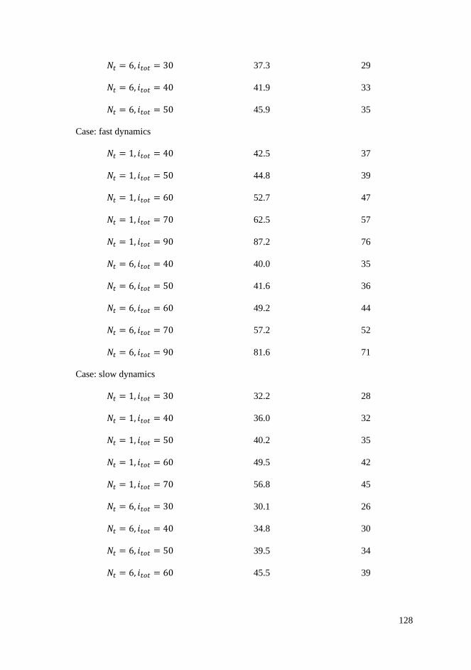
128
𝑁𝑡 = 6, 𝑖𝑡𝑜𝑡 = 30 37.3 29
𝑁𝑡 = 6, 𝑖𝑡𝑜𝑡 = 40 41.9 33
𝑁𝑡 = 6, 𝑖𝑡𝑜𝑡 = 50 45.9 35
Case: fast dynamics
𝑁𝑡 = 1, 𝑖𝑡𝑜𝑡 = 40 42.5 37
𝑁𝑡 = 1, 𝑖𝑡𝑜𝑡 = 50 44.8 39
𝑁𝑡 = 1, 𝑖𝑡𝑜𝑡 = 60 52.7 47
𝑁𝑡 = 1, 𝑖𝑡𝑜𝑡 = 70 62.5 57
𝑁𝑡 = 1, 𝑖𝑡𝑜𝑡 = 90 87.2 76
𝑁𝑡 = 6, 𝑖𝑡𝑜𝑡 = 40 40.0 35
𝑁𝑡 = 6, 𝑖𝑡𝑜𝑡 = 50 41.6 36
𝑁𝑡 = 6, 𝑖𝑡𝑜𝑡 = 60 49.2 44
𝑁𝑡 = 6, 𝑖𝑡𝑜𝑡 = 70 57.2 52
𝑁𝑡 = 6, 𝑖𝑡𝑜𝑡 = 90 81.6 71
Case: slow dynamics
𝑁𝑡 = 1, 𝑖𝑡𝑜𝑡 = 30 32.2 28
𝑁𝑡 = 1, 𝑖𝑡𝑜𝑡 = 40 36.0 32
𝑁𝑡 = 1, 𝑖𝑡𝑜𝑡 = 50 40.2 35
𝑁𝑡 = 1, 𝑖𝑡𝑜𝑡 = 60 49.5 42
𝑁𝑡 = 1, 𝑖𝑡𝑜𝑡 = 70 56.8 45
𝑁𝑡 = 6, 𝑖𝑡𝑜𝑡 = 30 30.1 26
𝑁𝑡 = 6, 𝑖𝑡𝑜𝑡 = 40 34.8 30
𝑁𝑡 = 6, 𝑖𝑡𝑜𝑡 = 50 39.5 34
𝑁𝑡 = 6, 𝑖𝑡𝑜𝑡 = 60 45.5 39

129
𝑁𝑡 = 6, 𝑖𝑡𝑜𝑡 = 70 56.0 45
4.2.3 Parametric effects
Analysis of the parametric effects would enhance the understanding of the model
behavior in turbulently flowing liquid-liquid dispersions particularly for oil-water flow in
pipes. To investigate the system behavior on the various parametric effects, the fitting
parameters are set to a new value as depicted in Table 4.5 below. In this new set of fitting
parameters, the variations of parameters in terms of energy dissipation rate, and volume
fraction, 𝜙 are assessed and evaluated.
Table 4.5 New fitting parameters
Parameter Value Descriptions
𝑘𝜔 1.70 𝑒 -03 Fitting parameter for coalescence frequency expression
𝑘𝜓 1.50 𝑒 -03 Fitting parameter for coalescence efficiency expression
𝑘𝑔1 2.50 𝑒 -02 Fitting parameter for breakage frequency expression
𝑘𝑔2 3.50 𝑒 -01 Fitting parameter for breakage efficiency expression
These parameters (i.e., 𝜙, and ) are crucial and contribute significantly to the
experimental strategies and design of the liquid-liquid two-phase pipe flow. For instance, in
experimental study of the overall drop size behaviour in two phase pipe flow, the typical
approaches are by changing and/or varying the fluid volume fraction (i.e., 𝜙) and the flow
conditions (i.e., 𝑈) of the system. In regard to the fluid volume fraction, altering the volume
fraction, 𝜙 of the dispersed phase will significantly affect the oil-water emulsion stability
(Meybodi et al., 2014). While, in the context of flow condition, changing the velocity is the
preferred method because of the direct influence on the turbulent kinetic energy in the system

130
which eventually leads to varying the energy dissipation rate, . The rate of energy
dissipation is estimated based on the newly proposed energy dissipation rate by Jakobsen
(2014). The rate is utilized based on the reason that the wall shear is the primary source of
turbulence production. Fig. 4.10 shows the effect of various energy dissipation rates, during
the drop size evolutions in terms of mean drop radii for number and volume density
distributions, 𝜇𝑁, and 𝜇𝑉. The results in Fig. 4.10 show that, at increase number of energy
dissipation rate, , the mean drop radii decreased and the magnitude is consistent approaching
the end of 1500m pipeline. Conversely, at low energy dissipation rate of = 2.0 m2/s3 the
mean radii are observed to be increased. These events are true considering that the energy
dissipation rate, is one of the primary mechanisms that control the breakage frequency as
depicted in Eqn. (3.17). Hence, due to an effect of small mean radii, the system will be
breakage dominated and high energy dissipation rate, . Conversely, if the mean radii are
large in magnitude, the system indicates coalescence dominated and low energy dissipation
rate, . As breakage becomes stronger due to increase in energy dissipation rate, , more
droplets will likely break into smaller droplets which leads to small magnitude in mean radii
as depicted in Fig. 4.10 (a) and (b). This is due to the increase in kinetic energy in the system
that eventually overcomes the surface energy of the droplets. Kumar et al., (1991) explained
that, droplets will deform and break under the influence of turbulent inertial stresses. In this
premise, increase in turbulent stresses will produce higher energy dissipation rate as a result
of high Reynolds number and consequently force the droplet to break and rupture. Solsvik et
al., (2017) also agreed that all droplets will break in turbulent liquid flows under high
Reynolds numbers and energy dissipation rate. Although, turbulent eddies is responsible for
breakup, however only large turbulent eddies from high energy dissipation rate contain
sufficient energy to affect breakage (Prince and Blanch, 1990). In general, the result on
parameter indicates that, the overall system behaviour can be in the form of breakage-

131
dominated or coalescence-dominated. The system is breakage-dominated if higher energy
dissipation rate is introduced (i.e., higher flow rate and Reynolds number) and coalescence-
dominated if the opposite criterion is met.
(a)
(b)
Figure 4.10 The effect of various energy dissipation rates, on the average radii of (a)
number density distribution, 𝜇𝑁 and (b) volume density distribution, 𝜇𝑉. The new fitting
parameters used are shown on top left corner of the plot.
Besides that, fitting parameters of 𝑘𝜔 and 𝑘𝑔1 are also important parameters to
evaluate because they can significantly affect the overall model behavior, particularly the
length of equilibrium, 𝐿𝑒𝑞. In this work, the 𝐿𝑒𝑞 is the length at which the mean radii are
consistently unchanged or equilibrated towards the end of the pipeline due to the balance
between the breakage and coalescence processes. Hence, to evaluate the effect of fitting
parameters 𝑘𝜔 and 𝑘𝑔1 on the overall system behaviour, the mean radii for number and

132
volume density distributions are plotted against the axial position, 𝑧 as depicted in Fig.
4.11(a) and (b). Furthermore, to maintain consistency in the study, the plot is selected at pipe
length 𝐿 = 10,000m and the fitting parameters 𝑘𝜔 and 𝑘𝑔1 are varied at three different order
of magnitudes (i.e., 10n where, n=-2,-3,-4). From Fig. 4.11, the system is found to equilibrate
at faster rate and shorter distance (shift to the left) as 𝑘𝜔 and 𝑘𝑔1 increase. Conversely, the
system is found to take slower time and longer equilibrium length (shift to the right) as 𝑘𝜔
and 𝑘𝑔1 decrease. The results indicate that the 𝑘𝜔 and 𝑘𝑔1 play a major role in altering and
controlling the equilibrium state of the system. In this respect, as the magnitude of 𝑘𝜔 and
𝑘𝑔1 increase, the equilibrium rate increases. This is true considering the intensity of the
coalescence and breakage rates generated as fitting parameters 𝑘𝜔 and 𝑘𝑔1 increase due to
direct proportionality effect of 𝑘𝜔 and 𝑘𝑔1 as depicted in Eqn. (3.11) and Eqn. (3.17). In
general, the results signify that, 𝑘𝜔 and 𝑘𝑔1 have a strong influence the overall system
behavior especially on the 𝐿𝑒𝑞. Hence, altering or changing these values one can gain control
on the relative magnitudes of coalescence and breakage frequencies which result in different
length of equilibrium.
(a)

133
(b)
Figure 4.11 The effect of fitting parameters 𝑘𝜔 and 𝑘𝑔1 at pipe length, 𝐿= 10,000m on the
average radii of (a) number density distribution, 𝜇𝑁 and (b) volume density distribution, 𝜇𝑉.
The last and most important parameter evaluated is the volume fraction of the oil-water
system, 𝜙. Fig. 4.12 shows the effect of various volume fractions on the mean number radii
as a function of axial position, 𝑧. The mean radii are found to be consistently growing until
they stabilize and level at a constant magnitude approaching the end of the pipeline (at higher
𝑧). The results of the mean radii in Fig. 4.12 indicates that, the volume fraction, 𝜙 plays a
major role in affecting the overall system behavior. In this regard, the bigger the volume
fraction, more droplets are expected to be present in the pipe and due to considerably high
coalescence frequency and efficiency parameters at about 𝑘𝜔= 1.70e-03 and 𝑘𝜓= 1.50e-03 in
the system, hence, the tendency to form larger droplets also increases. At these conditions,
the frequencies and chances of the droplets to collide and coalesce respectively are enhanced
particularly at high volume fraction. Experimental study by Maaß et al., (2012) on the effect
of dispersed phase fraction on drop size distributions supported the argument. They observed
that, the increase in dispersed phase fraction causes the mean drop sizes to increase. In a
nutshell, the magnitude of average drop radius becomes higher as volume fraction increased
at the given fitting parameters. Several authors relate this behavior due to turbulence damping
(Cohen 1991: Coulaloglou and Tavlarides, 1977), while, others attribute it to coalescence
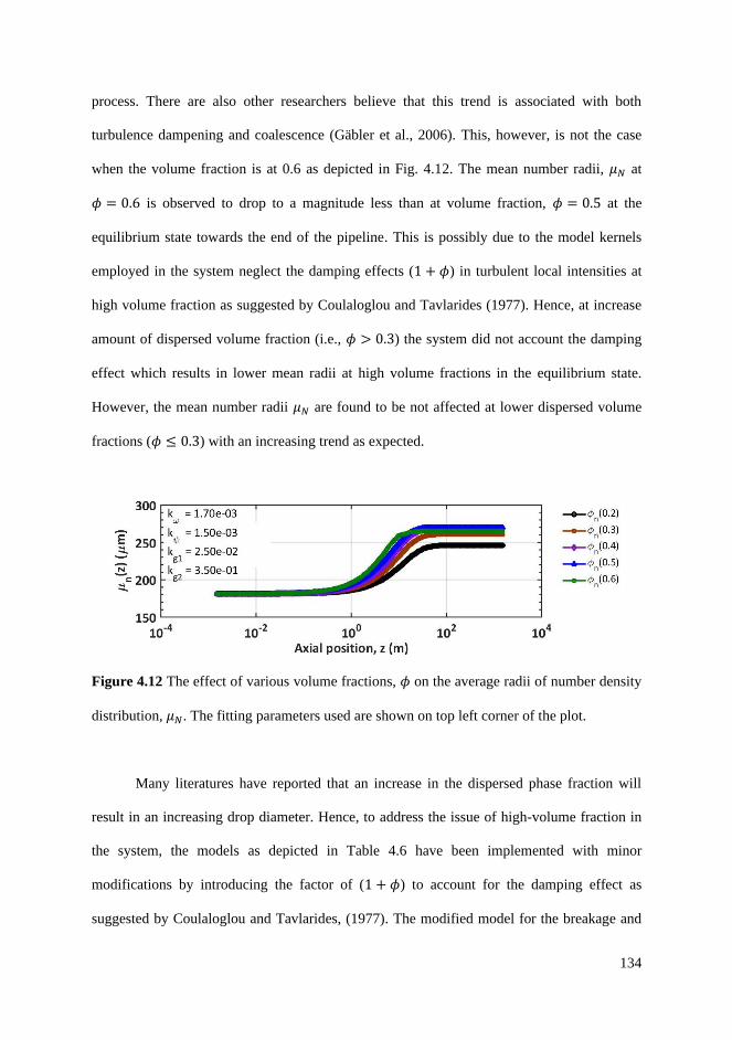
134
process. There are also other researchers believe that this trend is associated with both
turbulence dampening and coalescence (Gäbler et al., 2006). This, however, is not the case
when the volume fraction is at 0.6 as depicted in Fig. 4.12. The mean number radii, 𝜇𝑁 at
𝜙 = 0.6 is observed to drop to a magnitude less than at volume fraction, 𝜙 = 0.5 at the
equilibrium state towards the end of the pipeline. This is possibly due to the model kernels
employed in the system neglect the damping effects (1 + 𝜙) in turbulent local intensities at
high volume fraction as suggested by Coulaloglou and Tavlarides (1977). Hence, at increase
amount of dispersed volume fraction (i.e., 𝜙 > 0.3) the system did not account the damping
effect which results in lower mean radii at high volume fractions in the equilibrium state.
However, the mean number radii 𝜇𝑁 are found to be not affected at lower dispersed volume
fractions (𝜙 ≤ 0.3) with an increasing trend as expected.
Figure 4.12 The effect of various volume fractions, 𝜙 on the average radii of number density
distribution, 𝜇𝑁. The fitting parameters used are shown on top left corner of the plot.
Many literatures have reported that an increase in the dispersed phase fraction will
result in an increasing drop diameter. Hence, to address the issue of high-volume fraction in
the system, the models as depicted in Table 4.6 have been implemented with minor
modifications by introducing the factor of (1 + 𝜙) to account for the damping effect as
suggested by Coulaloglou and Tavlarides, (1977). The modified model for the breakage and

135
coalescence kernels are shown in Table 4.7 and the results are plotted in Fig. 4.13 using the
same fitting parameters plotted in Fig. 4.12 for the mean number radii, 𝜇𝑁.
Table 4.6 Existing model for breakage and coalescence kernels
Process Existing model
Breakage frequency
(Vankova et al., 2007)
𝑔(𝑟) = 𝑘𝑔1
1 3⁄
22 3⁄ 𝑟2 3⁄ √𝜌𝑐
𝜌𝑑𝑒𝑥𝑝 [−𝑘𝑔2
𝜎
𝜌𝑑25 3⁄ 𝑟5 3⁄ 2 3⁄]
Collision frequency
(Prince and Blanch,
1990)
𝜔𝑐(𝑟′, 𝑟′′) = 4√2
3𝑘𝜔
1 3⁄ (𝑟′ + 𝑟′′)2(𝑟′2 3⁄
+ 𝑟′′2 3⁄)1 2⁄
Coalescence efficiency
(Chesters, 1991)
𝜓𝐸(𝑟′, 𝑟′′) = exp [−𝑘𝜓
𝜌𝑐1 2⁄ 1 3⁄ 𝑟𝑒𝑞
5 6⁄
21 6⁄ 𝜎1 2⁄]
Table 4.7 Modified model for breakage and coalescence kernels
Process Modified model
Breakage frequency 𝑔(𝑟) = 𝑘𝑔1
1 3⁄
22 3⁄ 𝑟2 3⁄ (1 + 𝜙)√
𝜌𝑐
𝜌𝑑𝑒𝑥𝑝 [−𝑘𝑔2
𝜎(1 + 𝜙)2
𝜌𝑑25 3⁄ 𝑟5 3⁄ 2 3⁄]
Collision frequency 𝜔𝑐(𝑟′, 𝑟′′) =
4√2 3
𝑘𝜔1 3⁄
1 + 𝜙(𝑟′ + 𝑟′′)
2(𝑟′2 3⁄
+ 𝑟′′2 3⁄)1 2⁄
Coalescence efficiency 𝜓𝐸(𝑟′, 𝑟′′) = exp [−𝑘𝜓
𝜌𝑐1 2⁄ 1 3⁄ 𝑟𝑒𝑞
5 6⁄
21 6⁄ 𝜎1 2⁄ (1 + 𝜙)3]
Based on the coalescence and breakage models published in the literature (see Table
2.1 – 2.4), majority are found to neglect the damping factor (1 + 𝜙) on the local turbulent
intensities at high dispersed phase fraction as depicted in Table 4.6. Hence, this present work
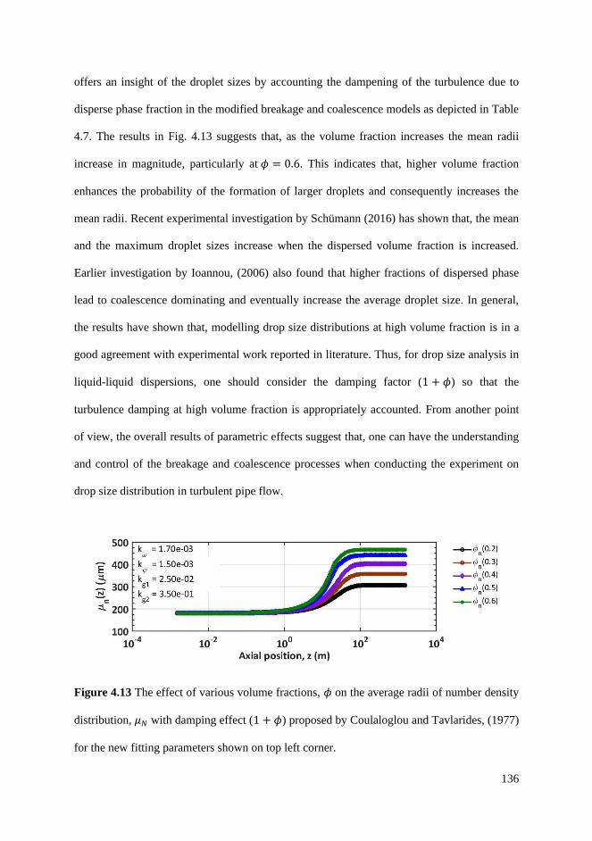
136
offers an insight of the droplet sizes by accounting the dampening of the turbulence due to
disperse phase fraction in the modified breakage and coalescence models as depicted in Table
4.7. The results in Fig. 4.13 suggests that, as the volume fraction increases the mean radii
increase in magnitude, particularly at 𝜙 = 0.6. This indicates that, higher volume fraction
enhances the probability of the formation of larger droplets and consequently increases the
mean radii. Recent experimental investigation by Schümann (2016) has shown that, the mean
and the maximum droplet sizes increase when the dispersed volume fraction is increased.
Earlier investigation by Ioannou, (2006) also found that higher fractions of dispersed phase
lead to coalescence dominating and eventually increase the average droplet size. In general,
the results have shown that, modelling drop size distributions at high volume fraction is in a
good agreement with experimental work reported in literature. Thus, for drop size analysis in
liquid-liquid dispersions, one should consider the damping factor (1 + 𝜙) so that the
turbulence damping at high volume fraction is appropriately accounted. From another point
of view, the overall results of parametric effects suggest that, one can have the understanding
and control of the breakage and coalescence processes when conducting the experiment on
drop size distribution in turbulent pipe flow.
Figure 4.13 The effect of various volume fractions, 𝜙 on the average radii of number density
distribution, 𝜇𝑁 with damping effect (1 + 𝜙) proposed by Coulaloglou and Tavlarides, (1977)
for the new fitting parameters shown on top left corner.

137
Additionally, simple regression analysis of drop size distribution at the final location
in the pipe is also evaluated to understand the overall model behavior. To demonstrate the
regression behavior, the sum of squares (SSQ) is evaluated between the simulation results
and the experimental results at the final location in the pipe. In general, the results from SSQ
enable important information in finding the best fit for the dynamic evolution of the drop size
density distribution in liquid-liquid emulsions in turbulent pipe flow. In this regression study,
the behavior of SSQ is plotted in terms of 𝑘𝜔 and 𝑘𝑔1 for three different values of fitting
parameters 𝑘𝜓 and 𝑘𝑔2 as depicted in Fig. 4.14(a), (b), and (c). The fitting parameters 𝑘𝜓 and
𝑘𝑔2 are set at decreasing in magnitude as shown in Fig. 4.14(a), (b), and (c), respectively. The
behavior of SSQ at 𝑘𝜓 =1.50e-02 and 𝑘𝑔2= 3.50e0 as portrayed in Fig. 4.19(a) indicates that
the local minima are lies in the region approaching the 10-4 of 𝑘𝑔1 and 100 for 𝑘𝜔. As shown
in this figure, the value for fitting parameters 𝑘𝜔 and 𝑘𝑔1 are set at lower, 𝑘𝜔 (i.e., ≤ 10-5)
and higher, 𝑘𝑔1 (i.e., ≥ 101). In this respect, for these set of fitting parameters (𝑘𝜓 and 𝑘𝑔2
),
one should avoid placing the higher and smaller values for the fitting parameters of, 𝑘𝑔1 and
𝑘𝜔, respectively, in order to find the best fit or local minima. On the other hand, Fig. 4.14(b)
provides significant information on finding the best fit. From these results of regression
behavior, one can have an insight on which order of magnitude and values of fitting
parameters in finding the best fit for the dynamic evolution of drop size distribution in
turbulently flowing liquid-liquid emulsions. In general, to find the best fit or local minima of
the system, one must consider the appropriate magnitude of 𝑘𝜓 and 𝑘𝑔2 (as depicted in Fig.
4.14(b)). This is because, the interplay between the four fitting parameters is crucial as they
are found to be significantly affecting the overall regression behavior.

138
(a)
(b)
(c)

139
Figure 4.14 The behavior of sum of squares (SSQ) as a function of 𝑘𝜔 and 𝑘𝑔1 at given
fitting parameters: (a) 𝑘𝜓= 1.50e-02 and 𝑘𝑔2= 3.50e-00, (b) 𝑘𝜓= 1.50e-03 and 𝑘𝑔2
= 3.50e-01, and
(c) 𝑘𝜓= 1.50e-04 and 𝑘𝑔2= 3.50e-02.
4.3 Chapter summary
This chapter discussed the drops evolution of oil-water emulsion in a long-distance
turbulent pipe flow. One of the main contributions in this present work is the proposed
solutions for the PBE. In this present work, the PBE is solved in the form of volume density
distribution, 𝑓𝑣 instead of the typical number density distribution, 𝑓𝑛. The study is also crucial
for case-specific system in a liquid-liquid condition with various fluids properties and flow
conditions. In this regard, the study on parametric effects provides the understanding on the
interplay between various parametric effects that contribute to the overall behavior of the
drop size distributions. Besides that, the model has proved to be reliable and robust from the
arbitrary set of results depicted. Two manuscripts are prepared (i.e.., Part I and Part II) for
this discussion (Chapter 4) as attached in Appendix B and C of this thesis. Next section will
discuss the regression of experimental pipe flow between simulation and experimental data.
140
CHAPTER 5
5 RESULTS AND DISCUSSION (PART II)
5.1 Part II: Regression of the experimental pipe flow data: comparison between
simulation and experimental data
In this chapter, the comparisons between the simulation and experimental data as well
as the best fitting parameters are analyzed and discussed. For the second part of the
discussions (Part II), the following physical properties of the oil-water system are used in the
simulation as depicted in Table 5.1. The physical properties shown in Table 5.1 are divided
into three different data sets known as ge12275a, ge12279a, and ge12284a. The primary
difference between the three experimental data sets is the average flow velocity, 𝑈. In this
respect, ge12275a represents the lowest average flow velocity, 𝑈 at 1.70 m/s, followed by
ge12279a and ge12284a with 2.0 m/s and 2.50 m/s, respectively. All the parameters in Table
5.1 are then used as inputs for the model simulations.
In this regression study, several models are selected for the breakage and coalescence
kernels in order to evaluate their effect on the dynamic evolution of the drop size density
distribution in pipes. The details of the models are summarized in Table 5.2, Table 5.3, and
Table 5.4. It is important to note that, the breakage kernels are selected based on the
mechanism of turbulent fluctuations. While, the coalescence kernels are selected from the
film drainage model and energy model as a result from turbulent-induced collisions. In Table
5.2, the selected models are categorized into three different cases known as case I, case II,
and case III. Each case comprised of different underlying mechanisms.

141
Table 5.1 Overview of the physical parameters from the experimental oil-water pipe flow
Parameter Ge12275a Ge12279a Ge12284a Descriptions
Ø 0.30 0.30 0.30 Volume fraction
𝑈 1.70 [m/s] 2.00 [m/s] 2.50 [m/s] Average flow velocity
𝐿 30 [m] 30 [m] 30 [m] Length of the pipe
𝑅𝑚𝑎𝑥 1000 [μm] 1000 [μm] 1000 [μm]
Upper bound of the radius
domain
𝐷 0.069 [m] 0.069 [m] 0.069 [m] Diameter of the pipe
𝜌𝑑 865 [kg/m3] 865 [kg/m3] 865 [kg/m3] Density of the dispersed phase
𝜇𝑑 177 [mPas] 169 [mPas] 152 [mPas] Viscosity of the dispersed phase
𝜌𝑐 1021 [kg/m3] 1021 [kg/m3] 1021 [kg/m3] Density of the continuous phase
𝜇𝑐 1.0 [mPas] 1.0 [mPas] 1.0 [mPas]
Viscosity of the continuous
phase
σ 26.0 [mN/m] 26.0 [mN/m] 26.0 [mN/m] Interfacial tension
Table 5.2 Comparison between simulation cases for breakage and coalescence kernels
Case Breakage kernels Coalescence kernels
I Coulaloglou and Tavlarides, (1977) +
Hsia and Tavlarides, (1980)
Coulaloglou and Tavlarides, (1977) +
Coulaloglou and Tavlarides, (1977)
II Vankova et al., (2007) + Coulaloglou
and Tavlarides, (1977)
Prince and Blanch (1990) + Chesters
(1991)
III Vankova et al., (2007) + Coulaloglou
and Tavlarides, (1977)
Prince and Blanch (1990) + Simon
(2004)

142
Table 5.3 Summary of breakage models for every case
Case Breakage kernels
I 𝑔(𝑟) = 𝑘𝑔1
1 3⁄
𝑟2 3⁄ (1 + 𝜙)exp [−𝑘𝑔2
𝜎(1 + 𝜙)2
𝜌𝑑2 3⁄ 𝑟5 3⁄
] +
𝛽(𝑟, 𝑟′) =45
2√23
𝑟2
𝑟′3(𝑟3
𝑟′3)
2
[1 − (𝑟3
𝑟′3)
2
]
II
𝑔(𝑟) = 𝑘𝑔1
1 3⁄
22 3⁄ 𝑟2 3⁄ √𝜌𝑑
𝜌𝑐𝑒𝑥𝑝 [−𝑘𝑔2
𝜎
𝜌𝑑25 3⁄ 𝑟5 3⁄ 2 3⁄] +
β(𝑟, 𝑟′) = 2.4
𝑟′3exp [−4.5
(2𝑟3 − 𝑟′3)2
𝑟′6] × 3𝑟2
III
𝑔(𝑟) = 𝑘𝑔1
1 3⁄
22 3⁄ 𝑟2 3⁄ √𝜌𝑑
𝜌𝑐𝑒𝑥𝑝 [−𝑘𝑔2
𝜎
𝜌𝑑25 3⁄ 𝑟5 3⁄ 2 3⁄] +
β(𝑟, 𝑟′) = 2.4
𝑟′3exp [−4.5
(2𝑟3 − 𝑟′3)2
𝑟′6] × 3𝑟2
Table 5.4 Summary of coalescence models for every case
Case Coalescence kernels
I 𝜔𝑐(𝑟
′, 𝑟′′ ) = 𝑘𝜔
ɛ1 3⁄
1 + 𝜙(𝑟′ + 𝑟′′ )2 [𝑟′2 3⁄
+ 𝑟′′ 2 3⁄ ]1 2⁄
+
𝜓𝑒(𝑟′, 𝑟′′ ) = exp [−
1
𝑘𝜓
𝜇𝑐𝜌𝑐
𝜎2(1 + 𝜙)3(
𝑟′𝑟′′
𝑟′ + 𝑟′′ )
4
]
II 𝜔𝑐(𝑟′, 𝑟′′) = 4√2
3𝑘𝜔
1 3⁄ (𝑟′ + 𝑟′′)2(𝑟′2 3⁄ + 𝑟′′2 3⁄ )
1 2⁄ +
𝜓𝑒(𝑟′, 𝑟′′) = exp [−𝑘𝜓
𝜌𝑐1 2⁄ 1 3⁄ 𝑟𝑒𝑞
5 6⁄
21 6⁄ 𝜎1 2⁄]
III 𝜔𝑐(𝑟′, 𝑟′′) = 4√2
3𝑘𝜔
1 3⁄ (𝑟′ + 𝑟′′)2 (𝑟′2 3⁄ + 𝑟′′2 3⁄ )
1 2⁄ +

143
𝜓𝑒(𝑟′, 𝑟′′) = exp [−
4𝑘𝜓𝜎(𝑟′2 + 𝑟′′2)
𝜌𝑑2 3⁄ 211 3⁄ (𝑟′11 3⁄ + 𝑟′′11 3⁄ )
]
There are various mechanisms discussed to describe the breakage process (refer to
Chapter 2, section 2.3.1 of this thesis) and the coalescence process (refer to Chapter 2, section
2.4.1 of this thesis) as explained in the review articles by Liao and Lucas (2009), Liao and
Lucas (2010), Sajjadi et al., (2013), Solsvik et al., (2013), and Abidin et al., (2015). However,
in this study, mechanism of turbulent fluctuations for breakage process is selected due to its
relevance applicability to the present study (i.e., liquid-liquid flow) as well as its extensive
used in the literature. Apart from limited discussions in literature, the other mechanisms such
as breakup due to viscous shear force, breakup due to shearing-off process, and breakup due
to interfacial instabilities are mainly developed based on gas-liquid system (Liao and Lucas,
2009).
On the other hand, for the coalescence process, the mechanism of turbulent-induced
collisions is selected. Wherein, other mechanisms such as droplets capture in an eddy,
velocity gradient-induced collisions, buoyancy-induced collisions, and wake interactions-
induced collision are primarily relevance only for gas-liquid system where the different in
properties of the phases are significant in affecting the collisions between bubbles/droplets.
Although there is an exception on drop collision mechanism of droplets capture in an eddy.
However, the mechanism is not able to predict the coalescence kinetics accurately as reported
by Sajjadi et al., (2013) and limited studies are found in the literature. Therefore, turbulent
fluctuations for breakage process and turbulent-induced collisions for coalescence process are
considered while, other mechanisms are not evaluated in the current work. The overview of
mechanisms for the simulation cases in each selected breakage and coalescence kernels are
illustrated in Table 5.5 as follows.

144
Table 5.5 Comparison between simulation cases based on underlying mechanisms for each
breakage and coalescence kernels
Case Mechanisms for breakage kernels Mechanisms for coalescence kernels
I Turbulent fluctuations + statistical
model (beta distribution function)
Turbulent-induced collisions + film
drainage model (deformable particles
with immobile interfaces)
II Turbulent fluctuations + statistical
model (normal distribution function)
Turbulent-induced collisions + film
drainage model (deformable particles
with fully mobile interfaces)
III Turbulent fluctuations + statistical
model (normal distribution function)
Turbulent-induced collisions + energy
model
In Table 5.5, the coalescence efficiency function in case I and case II are selected
based on film drainage model with specific characteristics of deformable droplets with
immobile interfaces and deformable droplets with mobile interfaces, respectively. In film
drainage, these characteristics are essential because they describe the quality of the
coalescence efficiency during the collision between two droplets, particularly in liquid-liquid
system. For both cases the deformable droplets refer to the rigidity of the particle surfaces,
while, the mobility denotes the motion of the colliding droplet interfaces during the process
of film drainage. In case I, the coalescence efficiency by film drainage is characterized by a
viscous thinning. Hence, this film drainage model is applicable for very viscous dispersed
phase or system with very specific surfactant soluble concentration (Liao and Lucas, 2010).
According to Lee and Hodgson (1968), the immobile interfaces refers to interfaces when the
surfaces shear stresses due to flow within the film are resisted by the interfacial tension
gradient set up because of expansion of the surface in the central regions of the film. In this

145
regard, the droplet can support an infinite high shear stress (Æther, 2002). This is due to the
presence of the surfactant or impurities at the interfaces and in this condition, the film will
drain very slowly (Æther, 2002). On the other hand, in case II, the coalescence efficiency
from the drainage process is the opposite criteria of case I. This model of deformable droplets
with fully mobile interfaces is suitable for a case of liquid-liquid system of the dispersed
phase (Chesters, 1991). In this respect, the drainage is no longer controlled by the viscous
stress as in immobile interfaces but instead by the resistance occurred in the film due to
deformation and acceleration (Chesters, 1991; Liao and Lucas, 2010).
5.2 Regression results and discussion (model validation with experimental data)
It is of interest in this section to compare the solution of the population balance
equation using various breakage and coalescence models against the three different
experimental data sets at the final location (pipeline). We used the fitting parameters to
determine the most robust and applicable coalescence or breakage models. Table 5.6 shows
the best estimation of the fitting parameters (i.e., 𝑘𝜔 , 𝑘𝜓, 𝑘𝑔1, 𝑘𝑔2
) for the regression of
experimental pipe flow data in terms of volume density distribution, 𝑓𝑣 at the final location.

146
Table 5.6 Numerical value of best fitting parameters and confidence intervals
Data set Case 𝑘𝜔 ± confidence interval 𝑘𝜓 ± confidence interval 𝑘𝑔1± confidence interval 𝑘𝑔2
± confidence interval
Ge12275a
I 2.200 × 10⁻² ± 5.19 × 10⁻⁵ 4.550 × 10⁻¹¹ ± 7.39 × 10⁻¹⁴ 3.879 × 10⁻¹ ± 6.27 × 10⁻⁴ 1.010 × 10⁻¹ ± 3.80 × 10⁻⁴
II 1.090 × 10⁻² ± 2.74 × 10⁻⁵ 8.499 × 10⁻³ ± 2.23 × 10⁻⁵ 1.870 × 10⁻¹ ± 4.70 × 10⁻⁴ 2.380 × 10⁻¹ ± 6.25 × 10⁻⁴
III 2.799 × 10⁻² ± 1.25 × 10⁻⁵ 1.100 × 10⁻⁴ ± 4.89 × 10⁻⁸ 4.750 × 10⁻¹ ± 7.93 × 10⁻⁴ 2.350 × 10⁻¹ ± 4.89 × 10⁻⁴
Ge12279a
I 2.550 × 10⁻² ± 1.30 × 10⁻⁵ 6.900 × 10⁻¹¹ ± 2.31 × 10⁻¹³ 4.050 × 10⁻¹ ± 2.69 × 10⁻⁴ 1.450 × 10⁻¹ ± 7.78 × 10⁻⁴
II 1.560 × 10⁻² ± 1.26 × 10⁻⁵ 5.500 × 10⁻³ ± 2.01 × 10⁻⁷ 2.460 × 10⁻¹ ± 1.90 × 10⁻⁵ 3.350 × 10⁻¹ ± 1.65 × 10⁻⁵
III 1.950 × 10⁻² ±1. 46 × 10−6 1.100 × 10⁻⁴ ± 6.02 × 10⁻⁷ 3.000 × 10⁻¹ ± 2.71 × 10⁻⁴ 3.250 × 10⁻¹ ± 2.16 × 10⁻⁵
Ge12284a
I 2.500 × 10⁻² ± 2.15 × 10⁻⁵ 9.850 × 10⁻¹¹ ± 1.07 × 10⁻¹³ 3.249 × 10⁻¹ ± 3.24 × 10⁻⁴ 2.150 × 10⁻¹ ± 1.95 × 10⁻⁴
II 1.059 × 10⁻² ± 2.60 × 10⁻⁷ 5.500 × 10⁻³ ± 1.40 × 10⁻⁷ 1.820 × 10⁻¹ ± 1.21 × 10⁻⁶ 6.149 × 10⁻¹ ± 3.72 × 10⁻⁶
III 3.200 × 10⁻² ± 5.94 × 10⁻⁶ 1.100 × 10⁻⁴ ± 1.73 × 10⁻⁷ 5.320 × 10⁻¹ ± 5.79 × 10⁻⁴ 5.850 × 10⁻¹ ± 1.46 × 10⁻⁴
147
It is worth noting that, each two of the fitting parameters are associated with
coalescence (𝑘𝜔 , 𝑘𝜓) and breakage (𝑘𝑔1, 𝑘𝑔2
) mechanisms, respectively. These four fitting
parameters are crucial as they control the dynamics of the overall system behaviour (as
discussed earlier in parametric effect in Part I of Chapter 4). The confidence intervals are
calculated based on the difference between the simulation and experimental data at the final
location of the pipes. The results tabulated in Table 5.6 also highlight the confidence intervals
that consist of the probability or the range limit of the best fitted parameters. From all of the
cases studied, the confidence interval is found to be at least one order of magnitude different
than the actual parameter. This suggests that, the results for the regression of breakage and
coalescence parameters at lower order of magnitude of the confidence interval are in good
agreement with the experimental data as shown in Fig. 5.1 until Fig. 5.3. The results of
regression clearly indicate that the model simulations are perfectly fit with the shape and peak
of the volume density distribution at final location in the pipeline for each of the best fitting
parameters depicted in Table 5.6. The comparison among all the cases and data sets suggests
that the fit of the drop volume distribution at the final location is considered satisfactory in
terms of the distribution properties (i.e., shape and peak location). This demonstrates that all
the models evaluated match the experimental data.

148
(a) (b)
(c)
Figure 5.1 Comparison of the scaled experimental volume density distribution and the model
prediction using the best fit parameters for case I and data set of: (a) ge12275a, (b) ge12279a,
and (c) ge12284a.

149
(a) (b)
(c)
Figure 5.2 Comparison of the scaled experimental volume density distribution and the model
prediction using the best fit parameters for case II and data set of: (a) ge12275a, (b)
ge12279a, and (c) ge12284a.

150
(a) (b)
(c)
Figure 5.3 Comparison of the scaled experimental volume density distribution and the model
prediction using the best fit parameters for case III and data set of: (a) ge12275a, (b)
ge12279a, and (c) ge12284a.
In this study, the fits are determined by using nonlinear regression model and while
doing so, the effect toward the overall model behavior have to be considered. For every
fitting parameter tested, the results are plotted and analyzed until it is considered to be
perfectly fits with the final (location) experimental data in terms of the shape and peak of the
volume density distribution. In addition to this approach, sum of squares (SSQ) are also
calculated to verify the best regression of the volume density distribution at final location.
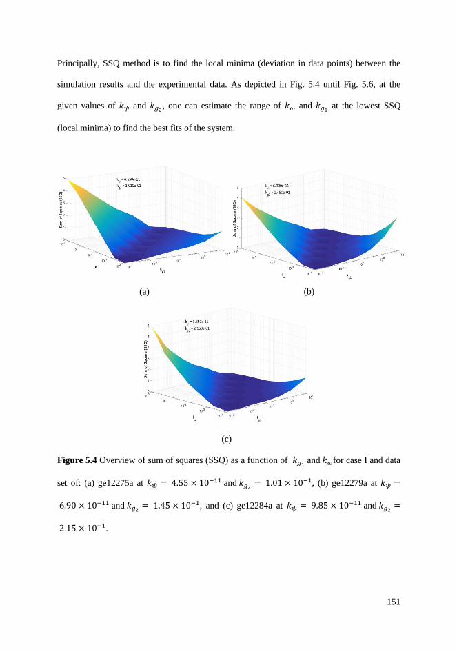
151
Principally, SSQ method is to find the local minima (deviation in data points) between the
simulation results and the experimental data. As depicted in Fig. 5.4 until Fig. 5.6, at the
given values of 𝑘𝜓 and 𝑘𝑔2, one can estimate the range of 𝑘𝜔 and 𝑘𝑔1
at the lowest SSQ
(local minima) to find the best fits of the system.
(a) (b)
(c)
Figure 5.4 Overview of sum of squares (SSQ) as a function of 𝑘𝑔1 and 𝑘𝜔for case I and data
set of: (a) ge12275a at 𝑘𝜓 = 4.55 × 10⁻¹¹ and 𝑘𝑔2= 1.01 × 10⁻¹, (b) ge12279a at 𝑘𝜓 =
6.90 × 10⁻¹¹ and 𝑘𝑔2= 1.45 × 10⁻¹, and (c) ge12284a at 𝑘𝜓 = 9.85 × 10⁻¹¹ and 𝑘𝑔2
=
2.15 × 10⁻¹.

152
(a) (b)
(c)
Figure 5.5 Overview of sum of squares (SSQ) as a function of 𝑘𝑔1 and 𝑘𝜔for case II and
data set of: (a) ge12275a at 𝑘𝜓 = 8.50 × 10⁻³ and 𝑘𝑔2= 2.38 × 10⁻¹, (b) ge12279a at
𝑘𝜓 = 5.50 × 10⁻³ and 𝑘𝑔2= 3.35 × 10⁻¹, and (c) ge12284a at 𝑘𝜓 = 5.50 ×
10−3 and 𝑘𝑔2= 6.15 × 10⁻¹.

153
(a) (b)
(c)
Figure 5.6 Overview of sum of squares (SSQ) as a function of 𝑘𝑔1 and 𝑘𝜔for case III and
data set of: (a) ge12275a at 𝑘𝜓 = 1.10 × 10⁻⁴ and 𝑘𝑔2= 2.35 × 10⁻¹, (b) ge12279a at
𝑘𝜓 = 1.10 × 10⁻⁴ and 𝑘𝑔2= 3.25 × 10⁻¹, and (c) ge12284a at 𝑘𝜓 = 1.10 ×
10−4 and 𝑘𝑔2= 5.85 × 10⁻¹.
The results of SSQ are tabulated in Table 5.7 along with the best fitting parameters for
all the cases and data sets studied. The results demonstrate that the calculated values of SSQ
from the function being fitted are in the range of ≈ 10−3 − 10−4, which indicates that the fits
are in good agreement with the experimental data as demonstrated in Fig. 5.1 until Fig. 5.3.
From Table 5.7, the best fitting parameter for collision frequency 𝑘𝜔 of this system is found
to be in the range between 1.00 × 10⁻² to 3.50 × 10⁻² for all the cases and data sets.

154
Table 5.7 Numerical value of the best fitting parameters for all the cases and data sets
Data set Case 𝑘𝜔 𝑘𝜓 𝑘𝑔1 𝑘𝑔2
𝑘𝑔1
𝑘𝜔 SSQ
Ge12275a
I 2.20 × 10⁻² 4.55 × 10⁻¹¹ 3.88 × 10⁻¹ 1.01 × 10⁻¹ 17.6 5.92 × 10⁻⁴
II 1.09 × 10⁻² 8.50 × 10⁻³ 1.87 × 10⁻¹ 2.38 × 10⁻¹ 17.1 6.32 × 10⁻⁴
III 2.80 × 10⁻² 1.10 × 10⁻⁴ 4.75 × 10⁻¹ 2.35 × 10⁻¹ 16.9 5.12 × 10⁻⁴
Ge12279a
I 2.55 × 10⁻² 6.90 × 10⁻¹¹ 4.05 × 10⁻¹ 1.45 × 10⁻¹ 15.9 8.50 × 10⁻⁴
II 1.56 × 10⁻² 5.50 × 10⁻³ 2.46 × 10⁻¹ 3.35 × 10⁻¹ 15.7 3.57 × 10⁻⁴
III 1.95 × 10⁻² 1.10 × 10⁻⁴ 3.00 × 10⁻¹ 3.25 × 10⁻¹ 15.3 6.06 × 10⁻⁴
Ge12284a
I 2.50 × 10⁻² 9.85 × 10⁻¹¹ 3.25 × 10⁻¹ 2.15 × 10⁻¹ 13.0 1.18 × 10⁻³
II 1.06 × 10⁻² 5.50 × 10⁻³ 1.82 × 10⁻¹ 6.15 × 10⁻¹ 17.1 6.22 × 10⁻⁴
III 3.20 × 10⁻² 1.10 × 10⁻⁴ 5.32 × 10⁻¹ 5.85 × 10⁻¹ 16.6 3.04 × 10⁻⁴
The fitting parameter for coalescence efficiency 𝑘𝜓 is expected to change for different
cases, however, in case I it is observed to be much smaller compared to the cases II and III.
This is owing to the fact that the model developed by Coulaloglou and Tavlarides, (1977)
assumed the initial thickness of the drops and the film thickness at which film rupture occurs
to be constant and lumped into parameter, 𝑘𝜓. Therefore, the fitting parameter 𝑘𝜓 carries a
unit of m2 and can take a very low magnitude (i.e., ≈ 10−10 − 10−20). It is important to
note that, in this present work, the equation by Coulaloglou and Tavlarides, (1977), 𝑘𝜓 is
treated as a denominator instead of numerator in the original model which we found to be
more practical and sensible in this system. The fitting parameter 𝑘𝜓 for case I is found to be
in the range of 4.00 × 10⁻¹¹ to 10.00 × 10⁻¹¹, while case II lies between 5.00 × 10⁻³
to 9.00 × 10⁻³ and case III, the parameter remains constant at 1.01 × 10⁻⁴. In other words,
the higher the value of 𝑘𝜓, the slower the coalescence rate become (the plot in Fig. 5.1 and
Fig. 5.3 will shift backward). This is due to the fact that, 𝑘𝜓 poses a direct proportionality

155
influence against the coalescence efficiency model in the exponential term (𝑘𝜓 as numerator)
as shown in Table 5.4 for all the cases except case I. Consequently, higher magnitude of 𝑘𝜓
will under-predict the final experimental drop volume density distribution aside from case I,
where 𝑘𝜓 is the denominator (imposes indirect proportionality to the coalescence efficiency)
in the exponential term of coalescence efficiency model (refer to Table 5.4).
The result for breakage parameters, 𝑘𝑔1 and 𝑘𝑔2
are observed to be in the range of
1.00 × 10⁻¹ − 5.50 × 10⁻¹ and 1.00 × 10⁻¹ − 6.50 × 10⁻¹, respectively. It is worth noting
that the constants between 𝑘𝑔1 and 𝑘𝜔 play an important role in finding the best fitting
parameters. This is true by considering the results of sum of squares (SSQ) analysis as
depicted in Fig. 5.4 until Fig. 5.6. The fitting parameters of 𝑘𝑔1 and 𝑘𝜔 are observed to have a
local minima at every order of magnitude (i.e., 10n where n = 1, 2, 3) for every set of best
fitting parameters in 𝑘𝜓 and 𝑘𝑔2. To put into another perspective, the ratio of 𝑘𝑔1
/𝑘𝜔 is
calculated as depicted in Table 5.7. The ratio may provide an insight on the difference in the
degree of magnitude between 𝑘𝑔1 and 𝑘𝜔 for every cases and data sets in order to achieve the
best fit between the simulation and experimental data of the system. Nevertheless, in this
study, we are not determining the absolute value of 𝑘𝑔1/𝑘𝜔 but only the ratio between both
parameters. This due to the different complexity and system application as well as variation
in terms of the model employed.
Apart from that, the evolution of number density distribution, 𝑓𝑛 and volume density
distribution, 𝑓𝑣 are determined from the best fitting parameters estimated in Table 5.7 and
plotted against droplet of radius, 𝑟 for nine different locations of the pipe length for case I, II,
and III as illustrated in Fig. 5.7, 5.8 and 5.9. The plots provide an overview on the dynamic
evolution of drop density distribution in terms of number and volume density distributions
(𝑓𝑛 and 𝑓𝑣) throughout 30m pipe length for all the three different cases (case I, II, and III) and
data sets (ge12275a, ge12279a, and ge12284a). From the dynamic evolution of number
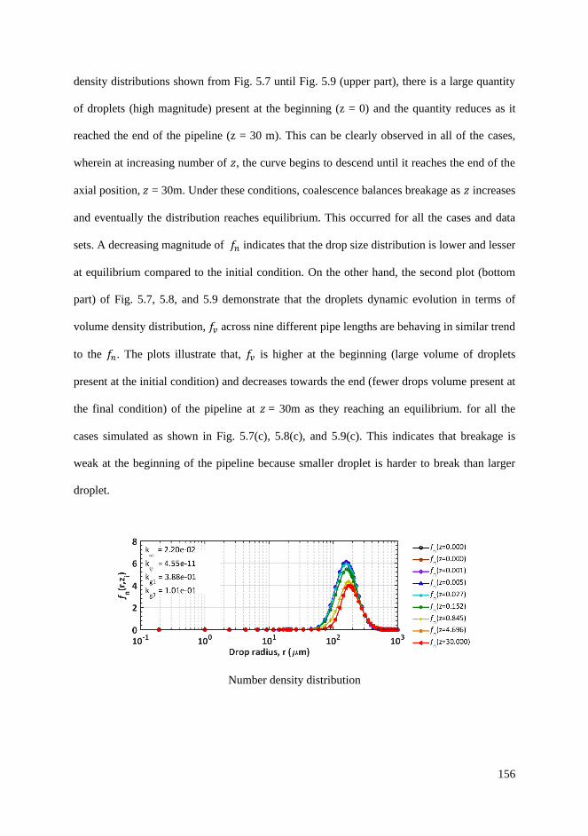
156
density distributions shown from Fig. 5.7 until Fig. 5.9 (upper part), there is a large quantity
of droplets (high magnitude) present at the beginning (z = 0) and the quantity reduces as it
reached the end of the pipeline (z = 30 m). This can be clearly observed in all of the cases,
wherein at increasing number of 𝑧, the curve begins to descend until it reaches the end of the
axial position, 𝑧 = 30m. Under these conditions, coalescence balances breakage as 𝑧 increases
and eventually the distribution reaches equilibrium. This occurred for all the cases and data
sets. A decreasing magnitude of 𝑓𝑛 indicates that the drop size distribution is lower and lesser
at equilibrium compared to the initial condition. On the other hand, the second plot (bottom
part) of Fig. 5.7, 5.8, and 5.9 demonstrate that the droplets dynamic evolution in terms of
volume density distribution, 𝑓𝑣 across nine different pipe lengths are behaving in similar trend
to the 𝑓𝑛. The plots illustrate that, 𝑓𝑣 is higher at the beginning (large volume of droplets
present at the initial condition) and decreases towards the end (fewer drops volume present at
the final condition) of the pipeline at 𝑧 = 30m as they reaching an equilibrium. for all the
cases simulated as shown in Fig. 5.7(c), 5.8(c), and 5.9(c). This indicates that breakage is
weak at the beginning of the pipeline because smaller droplet is harder to break than larger
droplet.
Number density distribution

157
Volume density distribution
(a)
Number density distribution
Volume density distribution
(b)
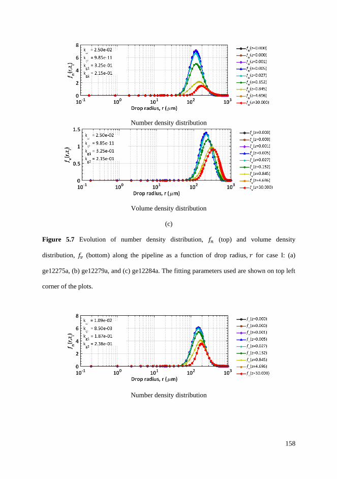
158
Number density distribution
Volume density distribution
(c)
Figure 5.7 Evolution of number density distribution, 𝑓𝑛 (top) and volume density
distribution, 𝑓𝑣 (bottom) along the pipeline as a function of drop radius, 𝑟 for case I: (a)
ge12275a, (b) ge12279a, and (c) ge12284a. The fitting parameters used are shown on top left
corner of the plots.
Number density distribution

159
Volume density distribution
(a)
Number density distribution
Volume density distribution
(b)
Number density distribution

160
Volume density distribution
(c)
Figure 5.8 Evolution of number density distribution, 𝑓𝑛 (top) and volume density
distribution, 𝑓𝑣 (bottom) along the pipeline as a function of drop radius, 𝑟 for case II: (a)
ge12275a, (b) ge12279a, and (c) ge12284a. The fitting parameters used are shown on top left
corner of the plots.
Number density distribution
Volume density distribution
(a)

161
Number density distribution
Volume density distribution
(b)
Number density distribution

162
Volume density distribution
(c)
Figure 5.9 Evolution of number density distribution, 𝑓𝑛 (top) and volume density
distribution, 𝑓𝑣 (bottom) along the pipeline as a function of drop radius, 𝑟 for case III: (a)
ge12275a, (b) ge12279a, and (c) ge12284a. The fitting parameters used are shown on top left
corner of the plots.
Besides that, to further investigate the changes in the droplets sizes as they travel
dynamically through the 30 m pipeline, the average radii profile of the drop density
distributions is plotted as depicted in Fig. 5.10(a) and (b). In this figure, the average radii for
the number and volume distributions (𝜇𝑛 and 𝜇𝑣) are plotted as a function of axial position, 𝑧
for all the three cases and data sets. The results in Fig. 5.10 show that, the average radii for
number density distribution, 𝜇𝑛 and volume density distribution, 𝜇𝑣 increased as the droplets
transport from the beginning towards the end of the pipeline. This indicates that, the
coalescence process is initially dominating over breakage in the overall system behavior due
to the increase in magnitude of the average radii (i.e., higher probability of droplets to
coalesce and forming larger droplets than breakup at the beginning of the pipe) for both
number and volume density distributions. The results are simulated based on the best fitting
parameters and initial distributions for each case. Aside that, from all the data sets evaluated,
data set ge12284a is found to experience higher relative change (i.e., larger magnitude of

163
mean radii) along the pipeline particularly at the equilibrium state (approaching the end of the
pipeline) compared to data sets ge12275a and ge12279a.
(a)
(b)
Figure 5.10 The average radii of (a) the number distribution, 𝜇𝑛 and (b) volume distribution,
𝜇𝑣 versus the axial position in the pipe, 𝑧 for all cases and data sets.
This is most likely owing to the different in magnitude of average flow velocity, 𝑈 in
all of the experimental data sets. In this respect, data set ge12284a contains the highest
average flow velocity, 𝑈 followed by data sets ge12279a and ge12275a. Hence, by taking this
into consideration and based on the initial condition, the data set ge12284a is expected to
experience greater kinetic energy from the turbulent eddies which ultimately leads to high
breakup of the droplets at the beginning of the pipe. This is due to the fact that, turbulent
kinetic energy supplied is sufficient or has exceeded the surface energy of the droplets. The
strong turbulent fluctuations in the flow means high energy dissipation rate and more droplets

164
are likely to break which results in higher 𝑓𝑛 and 𝑓𝑣 for small size droplets at the beginning of
the pipeline as depicted in Fig. 5.7, 5.8, and 5.9 (large quantity of smaller droplets at the
onset of the pipe). Schümann, (2016) supported the assumption in his experimental study of
oil-water pipe flow. He concluded that, higher mixture velocities increase the possibility of
the droplets to breakup and the droplet sizes decrease at higher velocity with increasing
Reynolds numbers. In this respect, more droplets will coalesce (high 𝜇𝑛 and 𝜇𝑣) and form due
to smaller sizes droplets produced at onset of the pipes. It worth noting that, In Fig. 5.10(a)
and (b), case II and case III are found to predict higher mean radii than case I for all the data
sets studied (i.e., ge12275a, ge12279a, ge12284a). This suggests that, the mechanisms
employed in the model for case II and case III have a tendency to predict high mean radii in
the system. This is because in case II, the coalescence efficiency by Chesters (1991) from the
film drainage model is considered from the deformable droplets at fully mobile interfaces
(see Fig. 2.11(c) in Chapter 2 of this thesis). In this context, the fully mobile interfaces are
expected to experience faster film drainage than case I at immobile interfaces (Æther, 2002).
In other words, the rate of coalescence efficiency is higher in case II resulting in larger mean
radii as demonstrated in Fig. 5.10(a) and (b). This process is suitable for a system having pure
fluids (i.e., no impurities or surfactants) or low viscosity fluids where viscous forces are
negligible (Chesters, 1991).
On the other hand, in case I, the film drainage model of deformable droplets at
immobile interfaces proposed by Coulaloglou and Tavlarides (1977) gives a lower magnitude
of mean radii in comparison to case II and III. This is owing to the model developed by
Coulaloglou and Tavlarides (1977) that takes into account the viscous stress effect from the
viscosity of the dispersed phase or/and specific surfactant soluble concentration in the system
(Liao and Lucas, 2010) as well as the effect of local turbulent intensities at high volume
fraction (1 + 𝜙). It is worth noting that, the effect of local turbulent intensities at high volume

165
fraction (1 + 𝜙) effectively reduces the rate of collision frequency (𝜔𝑐) due to the indirect
proportionality influence of the term as illustrated in Table 5.4. For these reasons, the
probabilities of droplets to form larger droplets are lower and resulting in small magnitude of
mean radii. Furthermore, if there is a presence of viscous effects at the interfaces, it is
expected that the drainage time will be sufficiently longer than the contact time, thus some
droplets may not be able to coalesce. As discussed by Kamp et al., (2017), in film drainage
model, the droplets must remain in contact for sufficient time until the intervening liquid film
thins to its critical thickness at which 𝑡𝑐𝑜𝑛𝑡𝑎𝑐𝑡 > 𝑡𝑑𝑟𝑎𝑖𝑛𝑎𝑔𝑒 (refer to Fig. 2.8 in Chapter 2 of
this thesis) for coalescence to occur. On the other hand, in case III, the coalescence efficiency
model proposed by Simon (2004) is strongly dependent on kinetic collision energy (as shown
in Table 5.4 for coalescence kernels). In this respect, the higher the kinetic energy (i.e.,
higher flow velocity, 𝑈) as described in data set ge12284a, the more efficient the coalescence
process will become (bigger droplet formed). Hence, the probability of coalescence (𝜓𝑒) from
drop collision process increases if the kinetic collision energy is greater than the surface
energy holding the droplet together (i.e., 𝐸𝑘 > 𝐸𝜎). Nevertheless, by taking into account the
complexity of the model and the turbulent flow behavior, the predictions (results) are
considered satisfactory based on the individual mechanisms as they appropriately described
the essence of droplets behavior in emulsion of oil and water. In addition, the results on
average radii may have important implication in terms of accessing designing strategies
specifically for multiphase separator system as well as droplet movement describing the
sedimentation and coalescence profiles (Jeelani and Hartland, 1998; Yu and Mao, 2004).
Apart from that, the simulations results in both figures (5.10a and 5.10b) also indicate
that the mean radii for number and volume density distributions (𝜇𝑛 and 𝜇𝑣) are approaching
equilibrium in which no significant net changes in drop sizes after they surpassed the 1 m
length of the pipe. In this case, the mean radii 𝜇𝑛 and 𝜇𝑣 are said to have equilibrate once

166
they reached the point where they are no longer growing (toward the end of the pipe length).
This is due to the fact that, the system is having a balance between the coalescence and
breakage processes. In this regard, the length at which the equilibrium achieved is called
𝐿𝑒𝑞 and it is set to the axial position of 𝑧-axis. Table 5.8 elucidates the length of equilibrium,
𝐿𝑒𝑞 based on the mean radii on each cases and pipe flow data for the set of best fitting
parameters (details in Table 5.7). Table 5.8 also calculates the time required for each length
once it reached the state of equilibrium. The length of equilibrium 𝐿𝑒𝑞 is an important
number to measure because it plays a major role in the overall system behaviour. The steady
and consistent magnitude of average drop radii approaching the end of the pipeline
determines how fast the system can achieve the length of equilibrium, 𝐿𝑒𝑞.
Table 5.8 Overview of length equilibrium, 𝐿𝑒𝑞 and time equilibrium, 𝑇𝑒𝑞 for number and
volume density distributions at every cases and data sets
Data set Case 𝐿𝑒𝑞𝑛 from 𝜇𝑛 𝐿𝑒𝑞𝑣 from 𝜇𝑣 𝑇𝑒𝑞𝑛
=𝐿𝑒𝑞𝑛
𝑈 𝑇𝑒𝑞𝑣
=𝐿𝑒𝑞𝑣
𝑈
Ge12275a
Case I 4.16 m 3.82 m 2.45 s 2.25 s
Case II 4.79 m 4.32 m 2.82 s 2.54 s
Case III 3.78 m 3.65 m 2.23 s 2.15 s
Ge12279a
Case I 4.79 m 4.35 m 2.39 s 2.18 s
Case II 5.52 m 4.66 m 2.76 s 2.33 s
Case III 3.62 m 3.34 m 1.81 s 1.67 s
Ge12284a
Case I 4.16 m 3.62 m 1.66 s 1.45 s
Case II 6.36 m 5.72 m 2.54 s
2.28 s
Case III 2.06 m 1.35 m 0.82 s 0.54 s

167
In a nutshell, the length of equilibrium, 𝐿𝑒𝑞 showed in Table 5.8 illustrates that the
time of equilibrium is influenced by the velocity, 𝑈. In this respect, with the increase of
velocity, 𝑈 from data set ge12275a to ge12284a, the system is observed to reach the
equilibrium at faster rate. Furthermore, the results also demonstrate that, case III has reached
the length of equilibrium, 𝐿𝑒𝑞 earlier compared to case I and case II. This is potentially due to
the energy model proposed by Simon, (2004) in the coalescence efficiency function and
combined with the turbulent fluctuation model from the breakage kernel which has greatly
affects the overall system behavior. In addition, case III consists of both coalescence and
breakage models developed from the similar mechanism of turbulent energy relationship.
Hence, as the turbulent energy increases particularly from data set ge12275a to ge12284a, the
equilibrium state of the system is accelerated. In other words, the higher the kinetic energy
supplied from the turbulent eddies, the faster the system is expected to reach the stability
(equilibrium). On the other hand, changing and altering the fitting parameters specifically the
𝑘𝜔 and 𝑘𝑔1 will also have a greater effect on the behavior of 𝐿𝑒𝑞. In this respect, the higher
the magnitude of fitting parameters 𝑘𝜔 and 𝑘𝑔1, the faster the system reaches equilibrium
(refer to Part I of Chapter 4 for details). This is mainly because of the direct effect on the rate
of breakage and coalescence frequencies as depicted in Table 5.3 and Table 5.4. Therefore,
the system will growth and equilibrates faster when the value of 𝑘𝜔 and 𝑘𝑔1are set at
substantially higher.
It is of interest in this study to investigate the dynamic evolution of drop density
distribution in terms of coalescence and breakage rates throughout the pipeline. To achieve
this, the best fit parameters shown in Table 5.7 are employed for every case to generate the
results related to the breakage and coalescence rates functions. Fig. 5.11 until Fig. 5.13,
illustrate the dynamic evolution of drop density distribution in terms of the total coalescence
rate (top), 𝑅𝐶𝑡 and total breakage rate (bottom), 𝑅𝐵𝑡
as a function of drop radius, 𝑟 at nine

168
different axial positions, 𝑧 in the 30 m pipe. The total rate is accounted for the birth and death
terms from the breakage and coalescence events. In these figures, the negative section of the
curves indicates the death of the droplets due to the coalescence and breakage processes,
while the positive section of the curves specifies the birth of the droplets owing to
coalescence and breakage developments. Essentially, the plots in Fig. 5.11 until 5.13 provide
an insight on the droplets behavior in terms of coalescence and breakage rates for all the
cases and data sets investigated. From these figures, it clearly shows that the total coalescence
rate is higher at the beginning of the pipeline and gradually decreases towards the end of the
pipeline. This is stemming from the fact that large quantity of smaller droplets initially
enhanced the collision rate between droplets. Moreover, film drainage is faster for small
droplets due to the small surface area and for droplets with low surface energy particularly,
for case I and II. While in case III, the efficiency of coalescence significantly increases with
increasing energy of collision (energy model) from the turbulent eddies (energetic collision)
as shown in data set ge12275a to data set ge12284a. It is worth noting that, case III produced
the highest birth rate of coalescence among the three cases and data sets simulated, which is
approximately in the range of 𝑅𝐶𝑡≈ 90 − 120 m-1s-1. This suggests that, case III has the
highest probability for coalescence to occur than case II and case I due to the higher
magnitude of total coalescence rate produced. By taking into account the mechanism of
energy-induced coalescence from the energy model by Simon, (2004), the coalescence
efficiency may have been strongly intensified in the system which results in significant
increase of overall total coalescence rate. Apart from that, at low 𝑟 values, the total
coalescence rate, 𝑅𝐶𝑡 is found to be in the negative section. This is expected because smaller
droplets present at the beginning of the pipeline are more likely to coalesce and forming
larger droplets. Subsequently, the larger droplets formed initially from the coalescence
process will breakup into smaller droplets (birth by breakage) as bigger droplets are more

169
likely to break than smaller ones. In general, 𝑅𝐶𝑡 is found to decrease as 𝑧 increases, which
indicates that the larger droplets formed during the coalescence process are breakup into
smaller droplets as breakage process becomes stronger towards the end of the pipeline until
both systems equilibrate. Further evidence of this observation stems from the fact that initial
droplets are too small to break which restricted the breakage process at the early stage of the
pipeline. However, as 𝑧 increases, breakage is growing in dominance because larger droplets
are more likely to break than coalesce.
Total coalescence rate
Total breakage rate
(a)
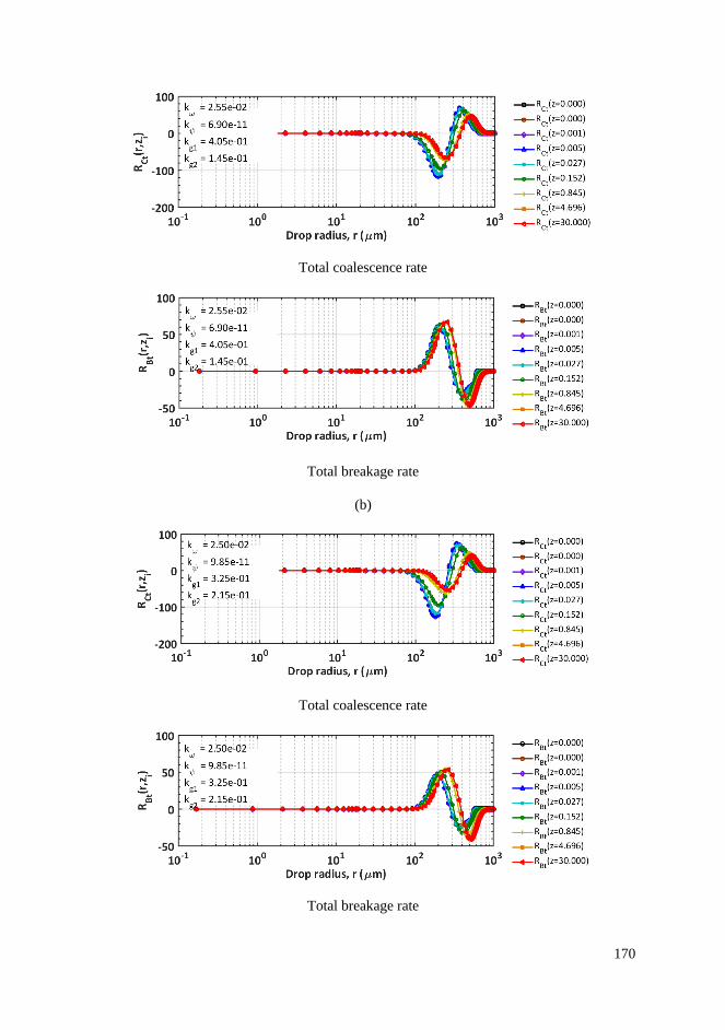
170
Total coalescence rate
Total breakage rate
(b)
Total coalescence rate
Total breakage rate

171
(c)
Figure 5.11 Evolution of the total coalescence rate 𝑅𝐶𝑡 (top) and evolution of the total
breakage rate, 𝑅𝐵𝑡 for case I and data set of: (a) ge12275a, (b) ge12279a, and (c) ge12284a.
Both rates are plotted as a function of droplet radius, 𝑟 at nine different locations in the pipe.
The fitting parameters used are shown on top left corner of the plots.
Total coalescence rate
Total breakage rate
(a)
Total coalescence rate

172
Total breakage rate
(b)
Total coalescence rate
Total breakage rate
(c)
Figure 5.12 Evolution of the total coalescence rate 𝑅𝐶𝑡 (top) and evolution of the total
breakage rate, 𝑅𝐵𝑡 for case II and data set of: (a) ge12275a, (b) ge12279a, and (c) ge12284a.
Both rates are plotted as a function of droplet radius, 𝑟 at nine different locations in the pipe.
The fitting parameters used are shown on top left corner of the plots.

173
Total coalescence rate
Total breakage rate
(a)
Total coalescence rate
Total breakage rate
(b)

174
Total coalescence rate
Total breakage rate
(c)
Figure 5.13 Evolution of the total coalescence rate 𝑅𝐶𝑡 (top) and evolution of the total
breakage rate, 𝑅𝐵𝑡 (bottom) for case III and data set of: (a) ge12275a, (b) ge12279a, and (c)
ge12284a. Both rates are plotted as a function of droplet radius, 𝑟 at nine different locations
in the pipe. The fitting parameters used are shown on top left corner of the plots.
The bottom sections of Fig. 5.11(a), (b), and (c), until Fig. 5.13(a), (b), and (c) show
the dynamic evolution of the drop density distribution in terms of total breakage rate in the 30
m pipeline for all the data sets and cases. As depicted in Fig. 5.11 until Fig. 5.13, the total
breakage rate, 𝑅𝐵𝑡 is found to have increased towards the end of the pipeline, in other words
𝑅𝐵𝑡 behaves in an exactly opposite trend to 𝑅𝐶𝑡
. The similar behaviour can be observed for all
the cases and data sets. This suggests that breakage becomes dominant and stronger as 𝑧
increases. Ideally, breakage occurs due to the interaction between the larger droplets and
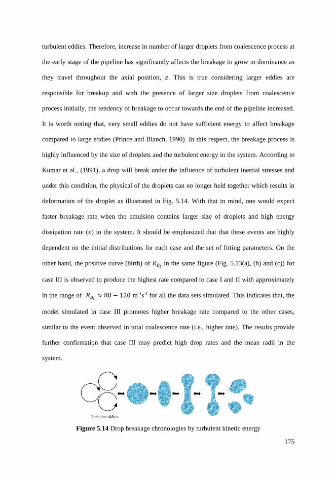
175
turbulent eddies. Therefore, increase in number of larger droplets from coalescence process at
the early stage of the pipeline has significantly affects the breakage to grow in dominance as
they travel throughout the axial position, 𝑧. This is true considering larger eddies are
responsible for breakup and with the presence of larger size droplets from coalescence
process initially, the tendency of breakage to occur towards the end of the pipeline increased.
It is worth noting that, very small eddies do not have sufficient energy to affect breakage
compared to large eddies (Prince and Blanch, 1990). In this respect, the breakage process is
highly influenced by the size of droplets and the turbulent energy in the system. According to
Kumar et al., (1991), a drop will break under the influence of turbulent inertial stresses and
under this condition, the physical of the droplets can no longer held together which results in
deformation of the droplet as illustrated in Fig. 5.14. With that in mind, one would expect
faster breakage rate when the emulsion contains larger size of droplets and high energy
dissipation rate ( ) in the system. It should be emphasized that that these events are highly
dependent on the initial distributions for each case and the set of fitting parameters. On the
other hand, the positive curve (birth) of 𝑅𝐵𝑡 in the same figure (Fig. 5.13(a), (b) and (c)) for
case III is observed to produce the highest rate compared to case I and II with approximately
in the range of 𝑅𝐵𝑡≈ 80 − 120 m-1s-1 for all the data sets simulated. This indicates that, the
model simulated in case III promotes higher breakage rate compared to the other cases,
similar to the event observed in total coalescence rate (i.e., higher rate). The results provide
further confirmation that case III may predict high drop rates and the mean radii in the
system.
Figure 5.14 Drop breakage chronologies by turbulent kinetic energy

176
5.3 Chapter summary
This chapter discussed the regression of the dynamic evolution of the drop size
density distribution of oil-water emulsion in a 30 m turbulent pipe flow. From the results, the
drop behavior over the turbulently flow in pipe are found to be very promising and the
models simulated have shown a good agreement with the experimental data. The fitting
parameters tested are fitted accordingly the drops volume density distribution at the final
location perfectly. The best fit results between the experimental data and simulation
demonstrated that the methodologies proposed in this modelling work (as discussed in
Chapter 3) have proved to be working effectively. Hence, the models can be considered
reliable and robust from all the results depicted. One manuscript (Part III) has been prepared
for this discussion and can be found in Appendix D of this thesis.

177
CHAPTER 6
6 CONCLUDING REMARKS
In this recent work, the dynamic evolution of the drop size density distribution of
liquid-liquid emulsions in turbulent pipe flow was investigated. The results and discussions
of this work are divided into two main parts, in which Part I covered the model behavior and
parametric effects and Part II discussed the comparison between the simulation and
experimental data for various breakage and coalescence models. In Part I of this research, the
general form of a mathematical model to simulate the dynamic evolution of drop size density
distribution in turbulently flowing liquid-liquid dispersions through pipeline was presented
using the method of population balance equation (PBE). In the context of model
development, possible methodology is elucidated incorporating the breakage process due to
turbulent fluctuations and coalescence process from the film drainage between droplets.
Moreover, the properties of the mixture liquids and the flow conditions are also incorporated
in order to understand the overall system behavior of the drop sizes evolution in liquid-liquid
dispersions. The model also suggests that the evolution of number density distribution,
volume density distribution, mean radii, standard deviations, total coalescence and breakage
rates, and total growth rates for a liquid-liquid system are take place in isotropic turbulence
condition at any position over a long distance pipeline. The performances of both breakage
and coalescence processes are presented based on how fitting parameters, 𝑘𝑔1 and 𝑘𝜔
𝑘𝜓 and 𝑘𝑔2 are change from case to case (i.e., case I, case II, and case III). In addition, for any
position in the pipeline, the model is able to simulate the evolution of breakage and
coalescence processes in terms of birth and death rates as well as their total growth rates. At
the same time, the advantages of solving the PBE in the form of volume density
distribution 𝑓𝑣 compared to number density distribution 𝑓𝑛 are also discussed as well as the

178
error analysis of using the spectral element in the orthogonal collocation method (i.e., 𝑁𝑡 =
6) to identify the best numerical solutions. One of the important contributions of this model
work is coming from the suggestion of converting the solution for PBE from number density
distribution 𝑓𝑛 to volume density distribution 𝑓𝑣. The results have shown that, solving the
PBE in the form of 𝑓𝑣 provide more stability and consistency to numerical solutions as
volume remains constant due to volume conservation, while, 𝑓𝑛 changed significantly during
drop growth process as number is not conserved (i.e., not consistent). In brief, the study
provides an insight of the modelling strategies and the solutions to the PBE towards
understanding and describing the overall system behavior of the drop size density distribution
in turbulently flowing liquid-liquid dispersions.
On top of that, the discussions in Part I (Chapter 4) of this thesis are continued with
the study of the model performance under various parametric effects to acquire understanding
and to elucidate the overall system behavior. In this respect, several parameters are varied
such as energy dissipation rate, , volume fraction, 𝜙, and four fitting parameters, 𝑘𝜔, 𝑘𝜓,
𝑘𝑔1, and 𝑘𝑔2
. The performances of both breakage and coalescence processes are also assessed
and evaluated based on these parametric effects. The model is also modified to incorporate
the damping effect with the factor of (1 + 𝜙) to account for turbulent intensities at high
volume fraction suggested by Coulaloglou and Tavlarides (1977). Overall, the results are
considered satisfactory as they are in good agreement with the experimental data and
theoretical studies. The results shown that, the mean radii increase as volume fraction
increases and decrease when energy dissipation rate increases. This is followed by
coalescence gradually growing in dominance as dispersed volume fraction increases and
conversely when energy dissipation rate is set higher. Apart from that, sum of squares (SSQ)
plots of the regression behavior are also presented and analyzed. The results indicate that the
interaction between all four fitting parameters is crucial in finding the best local minima. In

179
general, the four fitting parameters play an important role in changing the behavior of
coalescence and breakage models. Essentially, the study adds detail in understanding of the
interplay between various parametric effects on the coalescence and breakage mechanisms
and their relationship that contribute to the overall behavior of the drop size distributions. The
results are encouraging and provide useful information for the understanding of the model in
simulating and solving the dynamic evolution of liquid-liquid emulsions in turbulent pipe
flow.
Finally, the regression of experimental drop size density distribution in turbulent pipe
flow is investigated. In this present work, the performance of two different breakage kernels
and three separate coalescence kernels by Coulaloglou and Tavlarides (1977), Hsia and
Tavlarides (1980), Vankova et al., (2007), Prince and Blanch (1990), Chesters (1991), and
Simon (2004) are assessed and evaluated. The model and experimental data are directly
compared in terms of volume density distribution at final location in the pipe. Overall,
satisfactory agreement is observed in all of the model’s predictions with the experimental
pipe flow data. Based on the analysis of the results, turbulent fluctuation is the best
mechanism for breakage process, wherein, film drainage is the suitable mechanism to
describe for coalescence process particularly, in turbulently flowing oil-water emulsions in
pipe flow. However, discrepancies are discovered in terms of mean radii and total drop rate
predicted between the models studied. The models in Case III are found to promote higher
breakage and coalescence rates compared to case I and case II. Aside that, case II and case III
are found to produce higher mean radii in comparison to case I. The film drainage model
employed in case I from Coulaloglou and Tavlarides (1977) at immobile interfaces is found
to be the better model to describe the oil-water system in pipes. This is true considering that,
the model incorporates the viscous shear stress effect between two different liquids (viscous
liquid) as well as the effect from local volume fraction (1 + 𝜙). It is also worth noting that,

180
every model investigated in each case produced reasonable results for all the data sets of
different velocity conditions. However, one should expect differing in the magnitude of the
fitting parameters and higher mean radii as well as greater changes in total drop rate. In
addition, the model and experimental data indicate that the difference in degree of velocity
for data set of ge12275a, ge12279a, and ge12284a can affect the rate of coalescence and
breakage. That is, increased in velocity leads to higher coalescence and breakage rates as well
as faster equilibrium of mean radii (𝐿𝑒𝑞).

181
CHAPTER 7
7 SUGGESTIONS AND RECOMMENDATIONS FOR FUTURE WORK
It is recommended for the future work to study the dynamic evolution of the drop size
distribution by taking into account the aspects of angular and radial effects in the pipe flow. It
is because Schümann, (2016) and Lovick and Angeli (2004) have shown from the
experimental evidence that, droplets at the center of the pipe are larger than the droplets
found near the wall of the pipe. This is due to the fact that high shear rate close to the wall
promote the breakup process of the particles and leads to smaller droplet size. Another
essential aspect to consider in the future work is the physical state of the matter (i.e., gas,
liquid, solid). Variation in terms of the phases, for instance gas-liquid system may provide
profound understanding in modeling a more complicated three phase flow system (i.e., gas-
oil-water system or gas-liquid-solid system) which is becoming more common in the
industries, particularly in petroleum production. The study of gas-liquid system in turbulently
flowing pipeline will provide many significant information such that, the bubble size density
distribution, the interactions behaviour between bubbles in pipes, and the status of breakage
and coalescence rates in the system throughout the pipeline that benefitted the designs of
critical equipment such as multiphase separator.
Finally, is it also suggested that, one should consider the experimental data of drop
size density distribution (either number or volume density distribution) to be measured at the
midway of the pipeline apart from the inlet and the outlet. This measurement will provide
additional information of the drop size behaviour at the midway of the pipeline. Taking into
account the midway distribution will greatly contribute in finding the best fit at the final
location of the drop size density distribution. Hence, robust regression results can be
expected.

182
REFERENCES
Abidin, M. I. I. Z., Raman, A. A. A., Nor, M. I. M., 2015. Mean drop size correlations and
population balance models for liquid-liquid dispersion. AIChE. J. 61(4), 1129-1145.
Æther, L., 2002. Coalescence and breakup of drops and bubble. Ph.D. Dissertation.
Norwegian university of science and technology, NTNU, Norway.
Akinola, F., Borissova, A., Wang, X. Z., 2013. Extended method of moment for general
population balance models including size dependent growth rate, aggregation and
breakage kernels. Comp. Chem. Eng. J. 56, 1-11.
Alopaeus, V., Koskinen, J., Keskinen, K. I., 1999. Simulation of the population balances for
liquid-liquid systems in a nonideal tank. Part I Description and qualitative validation of
the model. J. Chem. Eng. Science. 54, 5887-5899.
Alopaeus, V., Koskinen, J., Keskinen, K. I., Majander, J., 2002. Simulation of the population
balances for liquid-liquid systems in a nonideal tank. Part II – parameter fitting and the
use of the multiblock model for dense dispersion. J. Chem. Eng. Science. 57, 1815-1825.
Alexopoulos, A.H., Roussos, A.I., Kiparissides, C., 2004. Part I: dynamic evolution of the
particle size distribution in particulate processes undergoing combined particle growth
and aggregation. J. Chemical Engineering Science. 59, 5751–5769.
Andersson, R., Andersson, B., 2006. On the breakup of fluid particles in turbulent flows,
AIChE J. 52, 2020-2030.
Angeli, P., Hewit, G. F., 1999. Flow structure in horizontal oil–water flow. Int. J. Multiphase
Flow 26, 1117–1140.
Arirachakaran, S., Oglesby, K. D., Malinowsky, M. S., Shoham, O., Brill, J. P., 1989. An
Analysis of oil/water flow phenomena in horizontal pipes. SPE-18836. Presented at the
SPE Production Operation Symposium, Oklahoma,U.S.A.

183
Asiagbe, K. S., 2018. Numerical simulation of gas-liquid bubbly flows. Ph.D. Thesis.
University of Leeds, UK.
Attarakih, M. M., Drumm, C., Bart, H. J., 2009. Solution of the population balance equation
using the sectional quadrature method of moments (SQMOM). J. Chem. Eng. Sci. 64,
742−752.
Azizi, F., Taweel, A, M., 2011. Turbulently flowing liquid-liquid dispersions. Part I: drop
breakage and coalescence. Chem. Eng. J. 166, 715-725.
Azizi, F., Taweel, A, M., 2010. Algorithm for the accurate numerical solution of PBE for
drop breakup and coalescence under high shear rates. Chem. Eng. Science J. 65, 6112-
6127.
Bilicky, Z., Kestin, J., 1987. Transition criteria for two-phase flow patterns in vertical upward
flow. Int. J. Multiphase Flow. 13, 283-294.
Becher, P., 2001. Emulsions: theory and practice. Third edition. Oxford university press,
New York, NY.
Bennett, M. K., Rohani, S., 2001. Solution of population balance equations with a new
combined Lax-Wendroff/Crank-Nicholson method. J. Chem. Eng. Sci. 56, 6623−6633.
Bochev, P., Gunzburger, M. D., 2009. Least-squares finite element methods. Springer, New
York.
Boxall, J. A., Koh, C. A., Sloan, E. D., Sum, A. K., Wu, D. T., 2010. Measurement and
Calibration of Droplet Size Distributions in Water-in-Oil Emulsions by Particle Video
Microscope and a Focused Beam Reflectance Method. Ind. Eng. Chem. Res. 49(3),
1412-1418.
Briceño, M., Salager, J. L., Bertrand, J., 2001. Influence of the dispersed phase content and
viscosity on the mixing of concentrated oil-in-water emulsions in the transition flow
regime. J. Chem. Eng. Res. Des. 79(8), 943-948.

184
Carrica, P. M., Drew, D., Bonetto, F., Lahey Jr, R. T., 1999. A polydispersed model for
bubbly two-phase flow around a surface ship. Int. J. Multiphase flow. 25, 257-305.
Chan, D. Y. C., Klaseboer, E., Manica, R., 2011. Film drainage and coalescence between
deformable drops and bubbles. Soft Matter J. 6, 2235-2264.
Chatzi, E., Lee, J. M., 1987. Analysis of interactions for liquid-liquid dispersions in Agitated
vessels. Ind. Eng. Chem. Res. 28, 1704-1711.
Chatzi, E., Gavrielides, A. D., Kiparissides, C., 1989. Generalized model for prediction of the
steady-state drop size distributions in batch stirred vessels. Ind. Eng. Chem. Res. 26(11),
2263-2267.
Chen, Z., Prüss, J., Warnecke, H. J., 1998. A population balance model for disperse systems:
drop size distribution in emulsion. Chem. Eng. Science. J. 53(5), 1059-1066.
Chesters, A. K., 1991. The modelling of coalescence processes in fluid-liquid dispersions. A
review of current understanding. J. Chem. Eng. Research and Design. 69, 259-270.
Clift, R., Grace, J. R., Weber, M. E., 1978. Bubbles, drops and particles, Academic press.
New York, USA.
Cristini, V., Blawzdziewicz, J., Loewenberg, M., Collins, L. R., 2003. Breakup in stochastic
Stokes flows: sub-Kolmogorov drops in isotropic turbulence. J. Fluid Mechanics. 492,
231–250.
Colin, C., Riou, X., Fabre, J., 2004. Turbulence and shear-induced coalescence in gas-liquid
pipe flows. Fifth international conference on multiphase flow. IMCF’04, Yokohama,
Japan. May 30 – June 4.
Coulaloglou, C.A., Tavlarides, L.L. 1977. Description of interaction processes in agitated
liquid-liquid dispersions. J. Chem. Eng. Science 32, 1289 -1297.
Davis, R. H., Schonberg, J. A., Rallison, J. M., 1989. The lubrication force between two
viscous drops. J. Physics of Fluids. 1, 77-81.

185
Deju, L., Cheung, S.C.P., Yeoh, G.H., Qi, F., Tu, J., 2015. Comparative analysis of
coalescence and breakage kernels in vertical gas-liquid flow.
DeRoussel, P., Khakhar, D. V., Ottino, J. M., 2001. Mixing of viscous immiscible liquids.
Part 1: Computational models for strong–weak and continuous 4ow systems. J. Chem.
Eng. Science; 56(19), 5511–5529.
Derjaguin, B. V., Kussakov, M. M., 1939. Anomalous properties of thin poly-molecular
films. Acta Physicochim. URRS. 10, 25-30.
Dorao, C. A., Jakobsen, H. 2006a. A least squares method for the solution of population
balance problems. J. Chem. Eng. Science. 30, 535-547.
Dorao, C. A., Jakobsen, H. 2006b. Application of the least-squares method for solving
population balance problems in ℝ𝑑+1. J. Chem. Eng. Science. 61, 5070-5081.
Dowding, P. J., Goodwin, J. W., Vincent, B., 2001. Factors governing emulsion droplet and
solid particle size measurements performed using the focused beam reflectance
technique. J. Coll. Surf. A: Phys. Eng. Aspects. 192, 5-13.
Eastwood, C. D., Armi, L., Lasheras, J. C., 2004. The breakup of immiscible fluids in
turbulent flows. J. Fluid Mechanics. 502, 309-333.
Elseth, G., 2001. An experimental study of oil-water flow in horizontal pipes. Ph.D. thesis.
Telemark University College, Porsgrunn, Norway.
Farr, R.S., 2013. Random close packing fractions of lognormal distributions of hard spheres.
Powder Technology. 245, 28-34.
Flores, J.G., Chen, X.T., Sarica, C., Brill, J. P., 1999. Characterization of oil/water flow
pattern in vertical and deviated wells. SPE-56108. SPE Prod. Facilities. 14(2), 102-109.
Flórez-Orrego, D., Arias, W., López, D., Velásquez, H. I., 2012. Experimental and CFD
study of a single-phase cone-shaped helical coiled heat exchanger: and empirical

186
correlation. Int. Conference. Eff. Cost. Opt. Sim. Env. Impact of Energy System. June
26-29. Perugia, Italy.
Friedlander, S. K., 1977. Smoke, Dust and Haze, Book, Wiley, New York.
Fu, X.Y., Ishii, M., 2002. Two-group interfacial area transport in vertical air-water flow: I.
Mechanistic model. Nucl. Eng. Des. 219(2),143–168.
Galinat, S., Masbernat, O., Guiraud, P., Dalmazzone, C., Nöik, C. 2005. Drop break-up in
turbulent pipe flow downstream of a restriction. J. Chem. Eng. Science. 60, 6511-6528.
Gavrielatos, I., Dabirian, R., Mohan, R. S., Shoham, O., 2017. Separation kinetics of
oil/water emulsions stabilized by nanoparticles. Preceeding, ASME, Fluids Eng. Division
Summer meeting, Waikoloa, Hawaii, USA.
Ghannam, H., Chahboun, A., Diani, M., Addou, M., 2017. Lattice Boltzmann simulations of
liquid drop shape on an inclined surface. Int. Conference. Auto. Control Eng. Comp.
Science (ACECS). Proceeding Eng. And Tech. 21, 9-13.
Grimes, B. A., 2011. Population balance model for batch gravity separation of crude oil and
water emulsions. Part I: model formulation. J. Disp. Science Tech. 33, 578-590.
Gunawan, R., Fusman, I., Braatz, R. D., 2004. High resolution for multidimensional
population balance equations. AIChE. J. 50(11), 2738-2749.
Hadnađev, T. D., Dokić, P., Krstonošić, Hadnađev, M., 2013. Influence of oil phase
concentration on droplet size distribution and stability of oil-in-water emulsions. Eur. J.
Lipid Sci. Technol. 115, 313-321.
Hagesaether, L., Jakobsen, H. A., Svendsen, H. F., 1999. Theoretical analysis of fluid particle
collisions in turbulent flow. Chem. Eng. Sci. 54, 4749-4755.
Hart, A., 2014. A review of technologies for transporting heavy crude oil and bitumen via
pipelines. J. Petrol. Explor. Prod. Technol. 4, 327-336.

187
Hemmingsen, P. V., Auflem, I. H., Sæther, Ø., Westvik, A., 2005. Emulsions and emulsion
stability: Droplet size distributions of oil-in-water emulsions under high pressures by
video microscopy. Taylor and Francis Group. Boca Raton, USA.
Hesketh, R. P., Etchells, A. W., Russell, T. W. F., 1991. Experimental observations of bubble
breakage in turbulent flow. J. Ind. Eng. Chem. Res. 30, 835-841.
Hinze, J. O., 1959. Turbulence. 2nd Edition. McGraw Hill. New York.
Howarth, W.J., 1964. Coalescence of drops in a turbulent flow field. J. Chem. Eng. Science.
19, 33-38.
Hulbert, H. M., Katz, S., 1964. Some problems in particle technology: a statistical
mechanical formulation. J. Chemical Engineering Science. 9, 555–574.
Hsia, M. A., Tavlarides, L. L., 1980. A simulation model for homogeneous dispersions in
stirred tanks. Chem. Eng. J. 20, 225-236.
Ioannou, K., 2006. Phase inversion phenomenon in horizontal dispersed oil/water pipeline
flows. Ph.D. Thesis. University College London, UK.
Ismail, A. S. I., Ismail, I., Zoveidavianpoor, M., Mohsin, R., Piroozian, A., Misnan, M. S.,
Sariman, M. Z., 2015a. Experimental investigation of oil–water two-phase flow in
horizontal pipes: Pressure losses, liquid holdup and flow patterns. J. Petroleum Sci. Eng.
127, 409-420.
Ismail, A. S. I., Ismail, I., Zoveidavianpoor, M., Mohsin, R., Piroozian, A., Misnan, M. S.,
Sariman, M. Z., 2015b. Review of oil-water through pipes. J. Flow Meas. Inst. 45, 357-
374.
Jakobsen, H. A., 2008. Chemical reactor modeling: multiphase reactive flows. Berlin,
Springer-Verlag.
Jakobsen, H. A., 2014. Chemical reactor modeling: multiphase reactive flows. Second
edition. Springer, Switzerland.

188
Jeelani, S. A. K., Hartland, S., 1998. Effect of dispersion properties on the separation of batch
liquid-liquid dispersions. Industrial. Eng. Chem. Res. 37(2), 547-554.
Jeelani, S. A. K., Hartland, S., 1991. Effect of approach velocity on binary and interfacial
coalescence. Chemical Engineering Research and Design: transactions of the institution
of chemical engineers: Part A 69, 271-281.
Jeffreys, G. V., Davies, G. A., 1971. Coalescence of liquid droplets and liquid dispersion.
Recent advances in liquid-liquid extraction book. Edited by: Handson, C. Pergamon
Press, New York. 495-584.
Jiang, B., 1998. The least-square finite element method: Theory and applications in
computational fluid dynamics and electromagnetics. Springer. Berlin.
John, V., Suciu, C., 2014. Direct discretizations of bi-variate population balance systems with
finite difference schemes of different order. J. Chem. Eng. Sci. 106, 39−52.
Karn, A., Shao, S., Arndt, R. E. A., Hong, J., 2016. Bubble coalescence and breakup in
turbulent bubbly wake of a ventilated hydrofoil. J. Exp. Thermal and Fluid Science. 70,
397-407.
Kamp, A. M., Chesters, A. K., Colin, C., Fabre, J., 2001. Bubble coalescence in turbulent
flows: A mechanistic model for turbulence-induced coalescence applied to microgravity
bubbly pipe flow. Int. J. Multiphase Flow. 27, 1363-1396.
Kamp, J., Villwock, J., Kraume, M., 2017. Drop coalescence in technical liquid/liquid
applications: a review on experimental techniques and modeling approaches. J. Review
in Chem. Eng. 33(1), 1-47.
Khatibi, M., 2013. Experimental study on droplet size of dispersed oil-water flow. Master
thesis. NTNU, Norway.
Kocamustafaogullari, G., Ishii, M., 1995. Foundation of the interfacial area transport equation
and its closure relations. Int. J. Heat and Mass Transfer. 38, 481-493.

189
Kokal, S., 2005. Crude-oils emulsion: state-of-the-art review. SPE production and facilities.
20, 5-13.
Komosawa, I., Otake, T., Kamojima, M., 1980. Wake behaviour and its effect on interaction
between spherical-cap bubbles. J. Chem. Eng. Japan. 13, 103-109.
Konno, M., Arai, K., Saito, S., 1983. Scale effect on breakup process in liquid-liquid agitated
tanks. J. Chem. Eng. Jpn. 16, 312-319.
Korovessi, E., Linninger, A. A., 2005. Batch processes. Book, CRC/Taylor and Francis
Group. NW. USA.
Kostoglou, M., Karabelas, A. J., 2007. On the breakage of liquid-liquid dispersions in
turbulent pipe flow: Spatial patterns of breakage intensity. J. Ind. Eng. Chem. Res. 46,
8220-8228.
Kumar, S., Kumar, R., Gandhi, K. S., 1991. Alternative mechanisms of drop breakage in
stirred vessels. Chem. Eng. Science J. 46(10), 2483-2489.
Kumar, S., Ramkrishna, D., 1997. On the solution of population balance equations by
discretization-III. Nucleation, growth and aggregation of particles. J. Chem. Eng.
Science. 52, 4659 – 4679.
Kumar, J., Warnecke, G., Peglow, M., Tsotsas, E., 2008. A note on sectional and finite
volume methods for solving population balance equations. Micro-Macro-Interactions in
structured media and particle systems. Editors: Bertram, A., Tomas, J. Springer.
Lane, G. L., Schwarz, M. P., Evans, G. M., 2005. Numerical modelling of gas-liquid flow in
stirred tanks. J. Chem. Eng. Science. 60, 2203-2214.
Lasheras, J. C., Eastwood, C., Martinez-Bazan, C., Montanes, J. L., 2002. A review of
statistical models for the break-up and immiscible fluid immersed into a fully developed
turbulent flow. Int. J. Multiphase Flow. 28, 247-278.

190
Lee, C. H., Erickson, L. E., Glasgow, L. A., 1987. Bubble breakup and coalescence in
turbulent gas-liquid dispersions. J. Chem. Eng. Comm. 59, 65-84.
Lee, J. C., Hodgson, T. D., 1968. Film flow and coalescence – I. Basic relation, film shape
and criteria for interface mobility. Chem. Eng. Science. 23, 1375-1387.
Lehr, F., Mewes, D., 1999. A transport equation for the interfacial area density in two-phase
flow. In: Second European Congress of Chemical Engineering, October 5-7, Montpellier,
France.
Lehr, F., Millies, M., Mewes, D., 2002. Bubble-size distributions and flow fields in bubble
columns. AIChE J. 48, 2426-2443.
Levich, V. G., 1962. Physiochemical hydrodynamics. Prentice Hall, Eaglewood Cliffs, NJ.
Liao, Y., Lucas, D., 2009. A literature review of theoretical models for drop and bubble
breakup in turbulent dispersions. J. Chem. Eng. Sci. 64, 3389-3406.
Liao, Y., Lucas, D., 2010. A literature review on mechanism and models for the coalescence
process of fluid particles. J. Chem. Eng. Sci. 65, 2851-2864.
Liao, Y., Rzehak, R., Lucas, D., Krepper, E., 2015. Baseline closure model for dispersed
bubbly flow: bubble coalescence and breakup. Chem. Eng. Science. 122, 336-349.
Lim, Y. I., Le Lann, J. M., Meyer, X. M., Joulia, X., Lee, G., Yoon, E. S., 2002. On the
solution of population balance equations (PBE) with accurate front tracking methods in
practical crystallization processes. J. Chem. Eng. Sci. 57, 3715−3732.
Liu, S., Li, D., 1999. Drop coalescence in turbulent dispersion. J. Chemical Engineering Sci.
54, 5667-5675.
Lovick, J., Angeli, P., 2004. Droplet size and velocity profiles in liquid-liquid horizontal
flows. J. Chemical Engineering Science. 59, 3105-3115.
Luo, H., 1993. Coalescence, breakup and liquid circulation in bubble column reactors. Ph.D.
Dissertation. Norwegian university of science and technology. Norway.

191
Luo, H., Svendsen, H. F., 1996. Theoretical model for drop and bubble breakup in turbulent
dispersions. AIChE J. 42(5), 1225- 1233.
Luo, H., Svendsen, H. F., 1996b. Modeling and simulation of binary approach by energy
conversation analysis. J. Chem. Eng. Communications. 145(1), 145-153.
Maaß, S., Gäbler, A., Zaccone, A., Paschedag, A. R., Kraume, M., 2007. Experimental
investigations and modeling of breakage phenomena in stirred liquid-liquid systems.
Chem. Eng. Res. Des. 85, 703-709.
Maaß, S., Wollny, S., Voigt, A., Kraume, M., 2011. Experimental comparison of
measurement techniques for drop size distributions in liquid/liquid dispersions. J. Exp.
Fluids. 50, 259-269.
Maaß, S., Paul, N., Kraume, M., 2012. Influence of the dispersed phase fraction on
experimental and predicted drop size distributions in breakage dominated stirred
systems. J. Chem. Eng. Science. 76, 140-153.
Maaß, S., Kraume, M., 2012. Determination of breakage rates using single drop experiments.
J. Chem. Eng. Science. 70, 146-164.
Maaß, S., Wollny, S., Voigt, A., Kraume, M., 2011. Experimental comparison of
measurement techniques for drop size distributions in liquid/liquid dispersions. J. Exp.
Fluids. 50, 259-269.
Marchisio, D. L., Fox, R. O., 2005. Solution of population balance equations using the direct
quadrature method of moments. J. Aerosol Sci. 36, 43-73.
Martínez-Bazán, C., Montañés, J. L., Lasheras, J. C., 1999. On the breakup of an air bubble
injected into a fully developed turbulent flow. J. Fluid Mech. 401, 157-182.
McGraw, R., 1997. Description of Aerosol Dynamics by the Quadrature Method of
Moments. Aerosol Sci. Technol. 27, 255-265.

192
Mesbah, A., Kramer, H. J. M., Huesman, A. E. M., Van den Hof, P. M. J., 2009. A control-
oriented study on the numerical solution of the population balance equation for
crystallization processes. J. Chem. Eng. Science. 64, 4262-4277.
Naeeni, S. K., Pakzad, L., 2019. Experimental and numerical investigation on mixing of
dilute oil in water dispersions in a stirred tank. J. Chem. Eng. Research and Design. 147,
493-509.
Narsimhan, G., 2004. Model for drop coalescence in a locally isotropic turbulent flow field. J
Colloid Interface Sci. 272,197–209
Narsimhan, G., Gupta, J.P., Ramkrishna, D., 1979. A model for transitional breakage
probability of droplets in agitated lean liquid-liquid dispersions. J. Chem. Eng. Sci. 34,
257-265.
Narsimhan, G., Ramkrishna, D., and Gupta, J.P., 1980. Analysis of drop size distributions in
lean liquid-liquid dispersions. AIChE Journal. 26, 991-1000.
Nere, N. K., Ramkrishna, D., 2005. Evolution of drop size distributions in fully developed
turbulent pipe flow of a liquid-liquid dispersion by breakage. Ind. Eng. Chem. Res. 44,
1187-1193.
Nere, N. K., Ramkrishna, D., 2006. Solution of population balance equation with pure
aggregation in developed turbulent pipe flow. J. Chem. Eng. Science. 61, 96-103.
Nguyen, T. T., Laurent, F., Fox, R., Massot, M., 2016. Solution of population balance
equations in applications with fine particles: mathematical modeling and numerical
schemes. J. Comp. Physics. 325, 129-156.
Oolman, T. O., Blanch, H. W., 1986. Bubble coalescence in stagnant liquids. Chemical
Engineering Communications. 43, 237-261.
Omar, H. M., Rohani, S., 2017. Crystal population balance formulation and solution methods:
a review. J. Crystal growth and design. ACS publications. 17(7), 4028-4041.

193
Opedal, N. V. D. T., SØrland, G., Sjöblom, J., 2009. Methods for droplet size distribution
determination of water-in-oil emulsions using low-field NMR. J. Basic Principles of
Diff. Theory, Exp. App. 9(7), 1-29.
Orrego, D. F., Arias, W., Lopez, D., Velasquez, H., 2012. Experimental and CFD study of a
single-phase cone-shaped helical coiled heat exchanger: an empirical correlation.
Proceedings of the International conference on efficiency, cost, optimization, simulation,
and environmental impact of energy systems, Perugia, Italy.
Otsubo, Y., Prud’homme, R. K., 1994. Effect of drop size distribution on the flow behaviour
of oil-in-water emulsions. Rheol. Acta J. 33(4), 303-306.
Pal, R., 1996. Effect of droplet size on the rheology of emulsions. AIChE J. 42(11), 3181-
3190.
Pal, R., Rhodes, E., 1989. Viscosity/concentration relationship for emulsions. Journal of
Rheology. 33, 1021-1045.
Park, J. Y., Blair, L. M., 1975. The effect of coalescence on drop size distribution in an
agitated liquid-liquid dispersion. J. Chem. Eng. Science. 30, 1057-1064.
Piela, K., Delfos, R., Ooms, G., Westerweel, J., Oliemans, R. V. A., Mudde, R. F., 2006.
Experimental investigation of phase inversion in oil-water flow through a horizontal
pipe. Int. J. Multiphase Flow. 32, 1087-1099.
Pinar, Z., Dutta, A., Bény, G., Öziş, T., 2015. Analytical solution of population balance
equation involving growth, nucleation and aggregation in terms of auxiliary equation
method. J. Applied Math. Info. Sciences. 9(5), 2467-2475.
Plasencia, J. 2013. Experimental study on two phase oil-water dispersed flow. Ph.D.
Dissertation. Norwegian university of science and technology. Norway.
Prince, M. J., Blanch, H. W., 1990. Bubble coalescence and break-up in air-sparged bubble
columns. AIChE J. 36()10, 1485-1499.

194
Prince, M. J., Walters, S., Blanch, H. W., 1989. Bubble break-up in air-sparged biochemical
reactors. In first generation of bioprocess engineering. Edited by Ghose, T.K.
Pumir, A., Wilkinson, M., 2016. Collisional aggregation due to turbulence. Annual review of
condensed matter physics. 7, 141-170.
Qamar, S., Wernecke, G., 2007. Numerical solution of population balance equations for
nucleation, growth and aggregation processes. J. Comp. Chem. Eng. 31, 1576-1589.
Raikar, N. B., Bhatia, S. R., Malone, M. F., McClements, D. J., Almeida-Rivera, C., Bongers,
P., Henson, A. M., 2010. Prediction of emulsion drop size distributions with population
balance equation models of multiple drop breakage. J. Colloids and Surfaces A:
Physicochemical and Eng. Aspects. 361, 96-108.
Raikar, N. B., Bhatia, S. R., Malone, M. F., Henson, M. A., 2009. Experimental studies and
population balance equation models for breakage prediction of emulsion drop size
distributions. J. Chem. Eng. Science. 64, 2433-2447.
Raikar, N. B., 2010. Prediction and manipulation of drop size distribution of emulsions using
population balance equation models for high pressure homogenization. PhD Thesis.
University of Massachusetts, U.S.A.
Ramkrishna, D. 1985. The status of population balances. Reviews for chemical engineering.
3(1), 49-95.
Ramkrishna, D. 2000. Population Balances: Theory and Applications to Particulate Processes
in Engineering. Academic Press, New York, NY.
Ramkrishna, D., Singh, M. R., 2014. Population balance modeling: current status and future
prospects. Annu. Rev. Chem. Biomol. Eng. J. 5, 123-146.
Ramadhan, H., Umar, Z., Sarieddine, M., Salama, G., Fahes, M., Nasrabadi, H., Manson, S.,
Haouche, M., Cheneviere, P., 2012. Study of oil/water emulsions in horizontal pipes.
Vol. EEP59, Qatar foundation annual research forum proceedings.

195
Randolph, A. D., 1964. A population balance for countable entities. Can. J. Chem. Eng.
42(6), 280–281.
Randolph, A.D., 1969. Effect of crystal breakage on crystal size distribution in a mixed
suspension crystallizer. Ind. Eng. Chem. Fund. 8, 58-63.
Randolph, A. D., Larson, M. A., 1988. Population balances: theory of particulate processes.
2nd edition. Analysis and techniques of continuous crystallization. Academic Press, San
Diego.
Rehman, S. M., Qamar, S., 2014. Application of the method of characteristics to population
balance models considering growth and nucleation phenomena. J. Applied mathematics.
5, 1853-1862.
Ribeiro, M. M., Regueiras, P. F., Guimarães, M. M. L., Madureira, C. M. N., Cruz_Pinto, J.
J. C., 2011. Optimization of breakage and coalescence model parameters in a steady-state
batch agitated dispersion. Ind. Eng. Chem. Res. 50, 2182-2191.
Rigopoulos, S., 2010. Population balance modelling of polydispersed particles in reactive
flows. J. Process in Energy and Combust. Science. 36, 412-443.
Rigopoulos, S., Jones, A. G., 2003. Finite element scheme for solution of the dynamic
population balance equation. A.I.Ch.E. Journal. (49),1127–1139.
Saboni, A., Gourdon, C., Chesters, A. K., 1995. Drainage and rupture of partially mobile
films during coalescence in liquid-liquid systems under a constant interaction force. J.
Colloid and Interface Science. 175, 27-35.
Salomon, D., 2011. The computer graphics manual. Springer, London, UK.
Sagert, N. H., Quinn, M. J., 1979. The coalescence of H2S and CO2 bubble in water.
Canadian J. Chem. Eng. 54, 392-398.

196
Sajjadi, B., Abdul Raman, A. A., Raja Ehsan Shah, R. S., Ibrahim, S., 2013. Review on
applicable breakup/coalescence models in turbulent liquid-liquid flows. Rev. Chem. Eng.
J. 29(3), 131-158.
Schramm, L. L. 1992. Petroleum Emulsions: Basic Principles in Emulsions: Fundamentals
and Applications in the Petroleum Industry. American Chemical Society, Washington,
DC.
Schümann, H., Khatibi, M., Tutkun, M., Pettersen, B. H., Yang, Z., Nydal, O. J., 2015.
Droplet size measurements in oil-water dispersions: A comparison study using FBRM
and PVM. J. of Dispersion Science and Tech. 1-45.
Schümann, H., 2016. Experimental investigation of transitional oil-water pipe flow. PhD
thesis. Norwegian university of science and technology (NTNU), Norway.
Schwartzberg, H., Treybal, R. E., 1968. Fluid and particle motion in turbulent stirred tanks.
Ind. Eng. Chem. Fundamen. 7(1), 1-6.
Simon, M., 2004. Koaleszenz von tropfen und tropfenschwärmen. Ph. D. Dissertation.
Technischen Universität Kaiserslautern. Germany.
Singh, P. N., Ramkrishna, D., 1977. Solution of population balance equations by MWR. J.
Comp. Chem. Eng. 1, 23-31.
Solsvik, J., Jakobsen, H. A., 2014. Bubble coalescence modeling in the population balance
framework. J. Dispersion Science and Tech. 35(11), 1626-1642.
Solsvik, J., Jakobsen, H. A., 2015. The foundation of the population balance equation: a
review. J. Dispersion Science and Tech. 36, 510-520.
Solsvik, J., Becker, P. J., Sheibat-Othman, N., Mohallick, I., Farzad, R., Jakobsen, H., 2015.
Viscous drop breakage in liquid-liquid stirred dispersions: population balance modeling.
J. Dispersion Science and Technol. 36(4), 577-594.

197
Solsvik, J., Borka, Z., Becker, P. J., Sheibat-Othman, N., Jakobsen, H., 2014. Evaluation of
breakage kernels for liquid-liquid systems: solution of the population balance equation
by the least-square method. Canadian. J. Chem. Eng. 92, 234-249.
Solsvik, J., Tangen, S., Jakobsen, H., 2013. On the constitutive equations for fluid particle
breakage. J. Rev. Chem. Eng. 29(5). 241-356.
Solsvik, J., Jakobsen, H. A., 2016. A review of the statistical turbulence theory required
extending the population balance closure models to the entire spectrum of turbulence.
AIChE. J. 62(5), 1795-1820.
Solsvik, J., Skjervold, V. T., Jakobsen, H. A., 2017. A bubble breakage model for finite
Reynolds number flows. J. Dispersion Science and Tech. 38(7), 973-978.
Søntvedt, T., Valle, A., 1994. Capacities of troll oil flow lines with high water cuts.
Predictions based upon recorded pipe flow friction factors for stable troll oil dispersions.
Report no. R-068557, Norsk Hydro ASA. Norway.
Sovova, H., 1981. Breakage and coalescence of drops in a batch stirred vessel II comparison
of model and experiment. J. Chem. Eng. Science. 36(9), 1567-1573.
Tsouris, C., Tavlarides, L. L., 1994. Breakage and coalescence models for drops in turbulent
dispersions. AIChE Journal. 40(3), 395-406.
Tsouris, C., Tavlarides, L. L., 2013. Fluid mechanics of mixing: modelling, operations, and
experimental techniques. Modelling and control of multistage mixer extractors. Bokk
edited by King, R. Springer science and business media.
Valentas, K.J., Bilous, O., Amundson, N.R., 1966. Analysis of breakage in dispersed phase
systems. I&EC Fundam. 5, 271 – 279.
Valentas, K. J., Amundson, N. R., 1966. Breakage and coalescence in dispersed phase
systems. Ind. Eng. Chem. Fundamen. 5(4), 533-542.

198
Vankova, N., Tcholakova, S., Denkov, N. D., Vulchev, V. D., Danner, T., 2007.
Emulsification in turbulent flow 2. Breakage rate constants. J. Colloid and Interface
Science. 313, 612-629.
Vay, K., Frieß, W., Scheler, S., 2012. Understanding reflection behavior as a key for
interpreting complex signals in FBRM monitoring of microparticle preparation
processes. Int. J. Pharmaceutics. 437, 1-10.
Von Smoluchowski, M., 1917.Versuch einer mathematischen theorie der Koagulationskinetik
kolloider LÖsungen. Z. Phys. Chem. 92, 129–68.
Villermaux, E., 2007. Fragmentation. J. Annual review fluid mechanics. 39, 419-446.
Vikas, V., Wang, Z. J., Fox, R. O., 2013. Realizable high-order finite-volume schemes for
quadrature-based moment methods applied to diffusion population balance equations, J.
Computational Physics. 249, 162-179.
Venneker, B. C. H., Derksen, J. J., Van Den Akker, H. E. A., 2002. Population balance
modeling of aerated stirred vessels based on CFD. AIChE J. 48(4), 673-685.
Vuong, D. H., Zhang, H. Q., Li, M., 2009. Experimental study on high viscosity oil/water
flow in horizontal and vertical pipes. In: SPE-124542-MS-P, SPE Annual Technical
Conference and Exhibition held in New Orleans, LA, U.S.A.
Wang, T., Wang, J., Jin, Y., 2005. Population balance model for gas-liquid flows: influence
of bubble coalescence and breakup models. Ind. Eng. Chem. Res. 44, 7540-7549.
Wang, G., Yang, F., Wu, K., Ma, Y., Peng, C., Liu, T., Wang, L.P., 2020. Estimation of the
dissipation rate of turbulent kinetic energy: a review. J. Chem. Eng. Science. 229, 116-
133.
Worlitschek, J., Buhr, J., 2005. Crystallization studies with focused beam reflectance
measurement and multimax. Application note. Mettler Toledo GmbH, AutoChem.

199
Yeoh, G. H., Cheung, C. P., Tu, J., 2014. Multiphase flow analysis using population balance
modeling. Book, Elsevier Ltd. UK.
Yuan, C., Laurent, F., Fox, R. O., 2012. An extended quadrature method of moments for
population balance equations. J. Aerosol Sci. 51, 1−23.
Yu, G. Z., Mao, Z. S., 2004. Sedimentation and coalescence profiles in liquid-liquid batch
settling experiments. Chem. Eng. Tech. 27, 407-413.
Zhang, J., Xu, S., Li, W., 2012. High shear mixers: A review of typical applications and
studies on power draw, flow pattern, energy dissipation and transfer properties. J. Chem.
Eng. and Processing. 57-58, 25-41.
Zhu, Z., Dorao, C. A., Jakobsen, H. A., 2008. A least-squares method with direct
minimization for the solution of the breakage–coalescence population balance equation.
J. Math. Computers. Sim. 79, 716-727.

200
APPENDIX A
DIMENSIONLESS ANALYSIS
A1 Dimensionless analysis
In order to transform the system equations into dimensionless form, five dimensionless
variables are introduced for the equations. These include dimensionless axial position in the
pipe, dimensionless radius of droplet, dimensionless drop volume, and dimensionless number
as well as volume number density distributions. For the scaling purposes, a characteristic
length and velocity are defined to transform the model into a dimensionless form. In this
respect, the characteristic length of the axial coordinate of the pipe (external coordinate) is
described as the total length of the pipe, 𝐿, and the characteristic velocity of the system is
defined as the average velocity in the pipe, 𝑈. On the other hand, the characteristic radius in
the scaling process is given by 𝑅𝑚𝑎𝑥 which describe the maximum size of drop radius in the
system. From the definitions above, the scaling relationships can be expressed as follows:
A1.1 Dimensionless variables:
(a) Dimensionless axial position in the pipe:
𝜆 =𝑧
𝐿 (1𝑎)
(b) Dimensionless radius (droplet):
𝜉 = 𝑟
𝑅𝑚𝑎𝑥 (2𝑎)

201
(c) Dimensionless drop volume:
�̅� =4
3𝜋𝑟3 = (
4
3𝜋𝑅𝑚𝑎𝑥
3 ) 𝜉3 = 𝑉𝑚𝑎𝑥𝜉3 (3𝑎)
The number density distribution 𝑓�̅� can be scaled from the definition of initial number density
distribution, 𝑁𝑑0 at the initial position in pipe (𝑧 = 0) as follows:
𝑁𝑑0(𝑧) = ∫ 𝑓𝑛0
𝑅𝑚𝑎𝑥
0
(𝑟′, 𝑧)𝑑𝑟′ (4𝑎)
(d) Dimensionless number density distribution:
𝑓�̅� = 𝑅𝑚𝑎𝑥
𝑁𝑑0𝑓𝑛 (5𝑎)
(e) Dimensionless volume density distribution:
𝑓�̅� = 𝑅𝑚𝑎𝑥 . 𝑓𝑣 (6𝑎)
Hence, from Eqn. (6a), the dimensionless number density distribution can be formulated in
terms of dimensionless volume density distribution as follows:
𝑓�̅� = 𝑓�̅�
𝑁𝑑0𝑉𝑚𝑎𝑥𝜉3 (7𝑎)
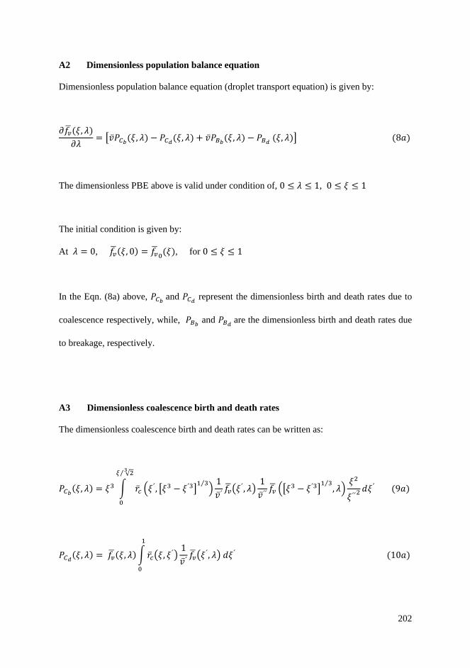
202
A2 Dimensionless population balance equation
Dimensionless population balance equation (droplet transport equation) is given by:
𝜕𝑓�̅�(𝜉, 𝜆)
𝜕𝜆= [�̅�𝑃𝐶𝑏
(𝜉, 𝜆) − 𝑃𝐶𝑑(𝜉, 𝜆) + �̅�𝑃𝐵𝑏
(𝜉, 𝜆) − 𝑃𝐵𝑑 (𝜉, 𝜆)] (8𝑎)
The dimensionless PBE above is valid under condition of, 0 ≤ 𝜆 ≤ 1, 0 ≤ 𝜉 ≤ 1
The initial condition is given by:
At 𝜆 = 0, 𝑓�̅�(𝜉, 0) = 𝑓�̅�0(𝜉), for 0 ≤ 𝜉 ≤ 1
In the Eqn. (8a) above, 𝑃𝐶𝑏 and 𝑃𝐶𝑑
represent the dimensionless birth and death rates due to
coalescence respectively, while, 𝑃𝐵𝑏 and 𝑃𝐵𝑑
are the dimensionless birth and death rates due
to breakage, respectively.
A3 Dimensionless coalescence birth and death rates
The dimensionless coalescence birth and death rates can be written as:
𝑃𝐶𝑏(𝜉, 𝜆) = 𝜉3 ∫ �̅�𝑐 (𝜉ˊ, [𝜉3 − 𝜉ˊ3]
1 3⁄)
𝜉 √23⁄
0
1
�̅�ˊ𝑓�̅�(𝜉
ˊ, 𝜆)1
�̅�ˊˊ𝑓�̅� ([𝜉3 − 𝜉ˊ3]
1 3⁄, 𝜆)
𝜉2
𝜉ˊˊ2𝑑𝜉ˊ (9𝑎)
𝑃𝐶𝑑(𝜉, 𝜆) = 𝑓�̅�(𝜉, 𝜆)∫ �̅�𝑐(𝜉, 𝜉
ˊ)1
�̅�ˊ
1
0
𝑓�̅�(𝜉ˊ, 𝜆) 𝑑𝜉ˊ (10𝑎)
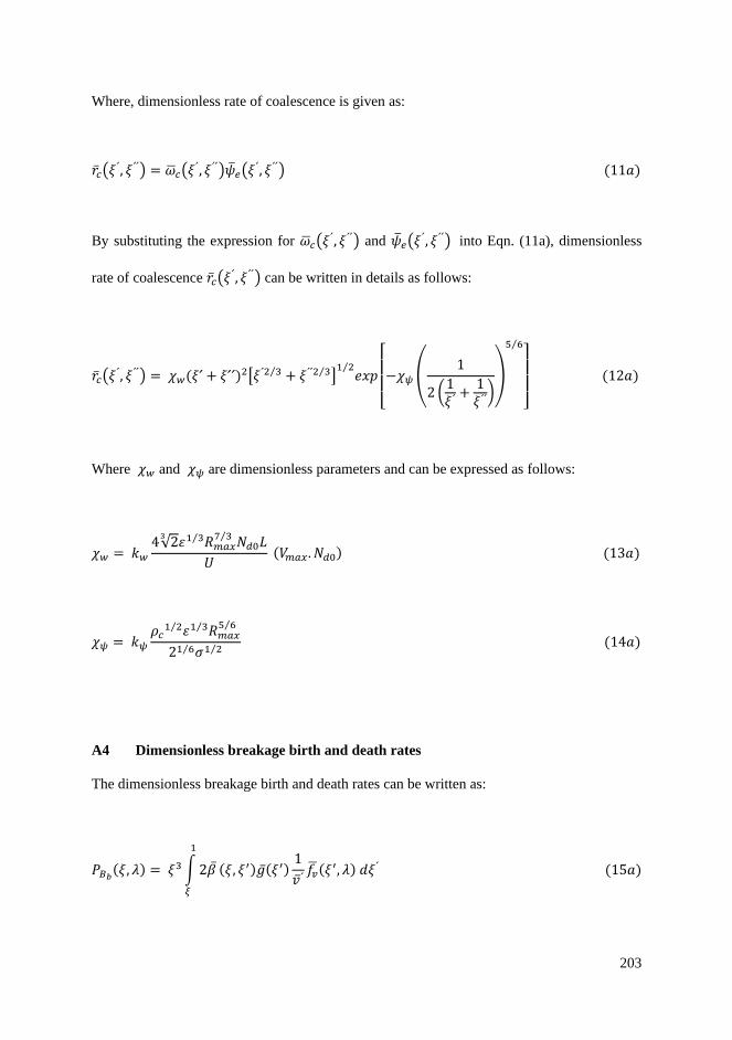
203
Where, dimensionless rate of coalescence is given as:
�̅�𝑐(𝜉ˊ, 𝜉ˊˊ) = �̅�𝑐(𝜉
ˊ, 𝜉ˊˊ)�̅�𝑒(𝜉ˊ, 𝜉ˊˊ) (11𝑎)
By substituting the expression for �̅�𝑐(𝜉ˊ, 𝜉ˊˊ) and �̅�𝑒(𝜉
ˊ, 𝜉ˊˊ) into Eqn. (11a), dimensionless
rate of coalescence �̅�𝑐(𝜉ˊ, 𝜉ˊˊ) can be written in details as follows:
�̅�𝑐(𝜉ˊ, 𝜉ˊˊ) = 𝜒𝑤(𝜉ˊ + 𝜉ˊˊ)2[𝜉ˊ2 3⁄ + 𝜉ˊˊ2 3⁄ ]
1 2⁄𝑒𝑥𝑝
[
−𝜒𝜓 (1
2 (1𝜉ˊ +
1𝜉ˊˊ)
)
5 6⁄
]
(12𝑎)
Where 𝜒𝑤 and 𝜒𝜓 are dimensionless parameters and can be expressed as follows:
𝜒𝑤 = 𝑘𝑤
4√23 1 3⁄ 𝑅𝑚𝑎𝑥
7 3⁄𝑁𝑑0𝐿
𝑈 (𝑉𝑚𝑎𝑥. 𝑁𝑑0) (13𝑎)
𝜒𝜓 = 𝑘𝜓
𝜌𝑐1 2⁄ 1 3⁄ 𝑅𝑚𝑎𝑥
5 6⁄
21 6⁄ 𝜎1 2⁄ (14𝑎)
A4 Dimensionless breakage birth and death rates
The dimensionless breakage birth and death rates can be written as:
𝑃𝐵𝑏(𝜉, 𝜆) = 𝜉3 ∫2�̅�
1
𝜉
(𝜉, 𝜉′)�̅�(𝜉′)1
�̅�ˊ𝑓�̅�(𝜉
′, 𝜆) 𝑑𝜉ˊ (15𝑎)

204
𝑃𝐵𝑑(𝜉, 𝜆) = [�̅�(𝜉) 𝑓�̅� (𝜉, 𝜆)] (16𝑎)
In Eqns. (15a) and (16a), the dimensionless rate of breakage, �̅�(𝑟) and dimensionless
daughter size distribution, �̅�(𝑟, 𝑟′) can be expressed as follows;
�̅�(𝑟) = 𝜒𝑔1
1
𝜉2 3⁄𝑒𝑥𝑝 [−𝜒𝑔2
15 3⁄
] (17𝑎)
�̅�(𝑟, 𝑟′) = 7.2 𝜉2
𝜉ˊ3𝑒𝑥𝑝 [−4.5
(𝜉3−𝜉ˊ3)2
𝜉ˊ6] (18𝑎)
Where 𝜒𝑔1 and 𝜒𝑔2 are dimensionless parameters and can be written as follows:
𝜒𝑔1 = 𝑘𝑔1
ɛ1 3⁄ 𝐿
𝑅𝑚𝑎𝑥2 3⁄ (1 + 𝜙)𝑈
(19𝑎)
𝜒𝑔2 = 𝑘𝑔2
𝛾(1 + 𝜙)2
𝜌𝑑ɛ2 3⁄ 𝑅𝑚𝑎𝑥5 3⁄
(20𝑎)
In Eqns. (13a) and (14a), the expression of 𝜒𝑤 represents the ratio of the residence time for a
drop in the pipe to the average time between droplet collisions. While the expression of 𝜒𝜓
indicates the ratio of the film drainage time constant to the droplet contact time constant.
Whereas, in Eqns. (19a) and (20a), the expression of 𝜒𝑔1 represents a comparison of the
droplet residence time in the pipe to the breakage time (frequency) of the drop in the
turbulent flow field. While, 𝜒𝑔2 signifies the ratio of the surface energy of the drop to the
mean turbulent kinetic energy in an eddy.

205
Substitute all the equations above for dimensionless coalescence and breakage processes into
the general equation shown in Eqn. (8a). Hence, the complete expression of dimensionless
population balance equation in terms of volume density distribution can be written as
follows:
𝜕𝑓�̅�(𝜉, 𝜆)
𝜕𝜆= 𝜉3 ∫
𝜉2
𝜉ˊˊ2�̅�𝑐 (𝜉ˊ, [𝜉3 − 𝜉ˊ3]
1 3⁄)
𝜉 √23⁄
0
1
�̅�ˊ𝑓�̅�(𝜉
ˊ, 𝜆)1
�̅� ˊˊ𝑓�̅� ([𝜉3 − 𝜉ˊ3]
1 3⁄, 𝜆) 𝑑𝜉ˊ
− 𝑓�̅�(𝜉, 𝜆)∫ �̅�𝑐(𝜉, 𝜉ˊ)
1
�̅�ˊ
1
0
𝑓�̅�(𝜉ˊ, 𝜆) 𝑑𝜉ˊ + 𝜉3 ∫2�̅�
1
𝜉
(𝜉, 𝜉′)�̅�(𝜉′)1
�̅�ˊ𝑓�̅�(𝜉
′, 𝜆) 𝑑𝜉ˊ
− [�̅�(𝜉) 𝑓�̅� (𝜉, 𝜆)] (21𝑎)
A5 Normalized number density, 𝑵𝒅̅̅ ̅̅ (𝝀) and dimensionless volume fraction, 𝝓(𝝀)
𝑁𝑑̅̅̅̅ (𝜆) =
𝑁𝑑(𝜆)
𝑁𝑑0= ∫𝑓�̅�(𝜉ˊ, 𝜆)
1
0
𝑑𝜉ˊ = ∫𝑓�̅��̅� ˊ
(𝜉ˊ, 𝜆)
1
0
𝑑𝜉ˊ (22𝑎)
𝜙(𝜆) = 𝑁𝑑0𝑉𝑚𝑎𝑥 ∫𝜉ˊ3𝑓�̅�(𝜉ˊ, 𝜆)
1
0
𝑑𝜉ˊ = ∫𝑓�̅�(𝜉ˊ, 𝜆)
1
0
𝑑𝜉ˊ (23𝑎)
A6 Dimensionless mean drop radii �̅�𝑵 and �̅�𝑽
�̅�𝑁(𝜆) =𝑅𝑚𝑎𝑥
𝑁𝑑̅̅̅̅ (𝜆)
∫𝜉ˊ𝑓�̅�(𝜉ˊ, 𝜆)
1
0
𝑑𝜉ˊ =𝑅𝑚𝑎𝑥
𝑁𝑑̅̅̅̅ (𝜆)
∫ 𝜉ˊ𝑓�̅��̅�ˊ
(𝜉ˊ, 𝜆)
1
0
𝑑𝜉ˊ (24𝑎)

206
�̅�𝑉(𝜆) = 𝑅𝑚𝑎𝑥
𝑁𝑑0
𝜙(𝜆)𝑉𝑚𝑎𝑥 ∫𝜉ˊ4𝑓�̅�(𝜉ˊ, 𝜆)
1
0
𝑑𝜉ˊ =𝑅𝑚𝑎𝑥
𝜙(𝜆)∫𝜉ˊ𝑓�̅�(𝜉
ˊ, 𝜆)
1
0
𝑑𝜉ˊ (25𝑎)
A7 Dimensionless standard deviation number, �̅�𝑵 and volume distributions, �̅�𝑽
𝜎𝑁(𝜆) = √𝑅𝑚𝑎𝑥
2
𝑁𝑑̅̅̅̅ (𝜆)
∫ (𝜉ˊ −�̅�𝑁
𝑅𝑚𝑎𝑥)2
𝑓�̅�(𝜉ˊ, 𝜆) 𝑑𝜉ˊ
1
0
= √𝑅𝑚𝑎𝑥
2
𝑁𝑑̅̅̅̅ (𝜆)
∫ (𝜉ˊ −�̅�𝑁
𝑅𝑚𝑎𝑥)2 𝑓�̅��̅� ˊ
(𝜉ˊ, 𝜆) 𝑑𝜉ˊ
1
0
(26𝑎)
𝜎𝑉(𝜆) = √𝑅𝑚𝑎𝑥2
𝑁𝑑0
𝜙(𝜆)𝑉𝑚𝑎𝑥 ∫(𝜉ˊ −
�̅�𝑉
𝑅𝑚𝑎𝑥)2
𝜉ˊ3𝑓�̅�(𝜉ˊ, 𝜆) 𝑑𝜉ˊ
1
0
= √𝑅𝑚𝑎𝑥
2
𝜙(𝜆)∫ (𝜉ˊ −
�̅�𝑉
𝑅𝑚𝑎𝑥)2
𝑓�̅�(𝜉ˊ, 𝜆) 𝑑𝜉ˊ
1
0
(27𝑎)
Apart from that, mass balance is also calculated to ensure that there are no droplets entering
or leaving the system during the simulation. This is crucial for the system to warrant the mass
remains conserve throughout the pipe lengths. The mass balance is determined by taking into
account the mass created and the mass disappeared from the coalescence and breakage
processes so that the condition is met for the following expressions:
𝑃𝐶𝑏(𝜉, 𝜆) − 𝑃𝐶𝑑
(𝜉, 𝜆) = 0 (28𝑎)

207
𝑃𝐵𝑏(𝜉, 𝜆) − 𝑃𝐵𝑑
(𝜉, 𝜆) = 0 (29𝑎)
The ratio of the coalescence mass balance 𝑀𝐶 is determined by dividing the dimensionless
volume integral for coalescence birth rate, 𝑃𝐶𝑏 against the dimensionless coalescence loss
rate, 𝑃𝐶𝑏. The same method applied to calculate the breakage mass balance, 𝑀𝐵 and both
ratios can be written as follows:
𝑀𝐶 =𝑃𝐶𝑏
(𝜉, 𝜆)
𝑃𝐶𝑑(𝜉, 𝜆)
(30𝑎)
𝑀𝐵 =𝑃𝐵𝑏
(𝜉, 𝜆)
𝑃𝐵𝑑(𝜉, 𝜆)
(31𝑎)
To ensure that the local volume fraction, ϕ remains constant, the mass balance ratio for both
coalescence and breakage, 𝑀𝐶 and 𝑀𝐵 are multiplied by the dimensionless coalescence and
breakage birth rates, 𝑃𝐶𝑏 and 𝑃𝐵𝑏
respectively, as written below:
𝑃𝐶𝑏= 𝑃𝐶𝑏
× 𝑀𝐶 (32𝑎)
𝑃𝐵𝑏= 𝑃𝐵𝑏
× 𝑀𝐵 (33𝑎)

208
APPENDIX B
(1st MANUSCRIPT)
This paper is awaiting publication and is not included in NTNU Open

271
APPENDIX C
(2nd MANUSCRIPT)
This paper is awaiting publication and is not included in NTNU Open

306
APPENDIX D
(3rd MANUSCRIPT)
This paper is awaiting publication and is not included in NTNU Open

ISBN 978-82-326-5407-9 (printed ver.)ISBN 978-82-326-5403-1 (electronic ver.)
ISSN 1503-8181 (printed ver.)ISSN 2703-8084 (online ver.)
Doctoral theses at NTNU, 2021:94
Ahmad Shamsulizwan Bin Ismail
Modeling the dynamic evolutionof drop size density distributionof the oil-water emulsion inturbulent pipe flow
Doc
tora
l the
sis
Doctoral theses at N
TNU
, 2021:94Ahm
ad Shamsulizw
an Bin Ismail
NTN
UN
orw
egia
n U
nive
rsity
of S
cien
ce a
nd T
echn
olog
yTh
esis
for t
he D
egre
e of
Philo
soph
iae
Doc
tor
Facu
lty o
f Nat
ural
Sci
ence
sD
epar
tmen
t of C
hem
ical
Eng
inee
ring
Related Documents