Modeling stabilizing selection: expanding the Ornstein-Uhlenbeck model of adaptive evolution

ORIGINAL ARTICLE

doi:10.1111/j.1558-5646.2012.01619.x

MODELING STABILIZING SELECTION:EXPANDING THE ORNSTEIN–UHLENBECKMODEL OF ADAPTIVE EVOLUTIONJeremy M. Beaulieu,1,2 Dwueng-Chwuan Jhwueng,3,4 Carl Boettiger,5 and Brian C. O’Meara6

1Department of Ecology and Evolutionary Biology, Yale University, P.O. Box 208106, New Haven, Connecticut 06520–81062E-mail: [email protected]

3National Institute for Mathematical and Biological Synthesis, 1534 White Ave, University of Tennessee, Knoxville,

Tennessee, 37996–15274Department of Statistics, Feng-Chia University, Taichung, Taiwan 40724, R.O.C.5Center for Population Biology, University of California, Davis, 1 Shields Avenue, Davis, California, 956166Department of Ecology and Evolutionary Biology, University of Tennessee, Knoxville, Tennessee, 37996–1610

Received September 2, 2011

Accepted February 6, 2012

Comparative methods used to study patterns of evolutionary change in a continuous trait on a phylogeny range from Brownian

motion processes to models where the trait is assumed to evolve according to an Ornstein–Uhlenbeck (OU) process. Although

these models have proved useful in a variety of contexts, they still do not cover all the scenarios biologists want to examine. For

models based on the OU process, model complexity is restricted in current implementations by assuming that the rate of stochastic

motion and the strength of selection do not vary among selective regimes. Here, we expand the OU model of adaptive evolution

to include models that variously relax the assumption of a constant rate and strength of selection. In its most general form, the

methods described here can assign each selective regime a separate trait optimum, a rate of stochastic motion parameter, and a

parameter for the strength of selection. We use simulations to show that our models can detect meaningful differences in the

evolutionary process, especially with larger sample sizes. We also illustrate our method using an empirical example of genome

size evolution within a large flowering plant clade.

KEY WORDS: Brownian motion, comparative method, continuous characters Hansen model, Ornstein–Uhlenbeck.

Single-rate Brownian motion works reasonably well as a modelfor evolution of traits. It models drift, drift-mutation balance, andeven stabilizing selection toward a moving optimum (Hansen andMartins 1996). However, a single parameter model can certainlynot explain the evolution of traits across all life. There have beenextensions to the model, such as a single Ornstein–Uhlenbeck(OU) process that has a constant pull toward an optimum value, amultiple mean OU process with different possible means for dif-ferent groups (Hansen 1997; Butler and King 2004), and multiplerate Brownian motion processes allowing different rates of evo-lution on different branches (O’Meara et al. 2006; Thomas et al.2006). These models, while useful, still do not cover all the sce-narios biologists want to examine. For example, existing modelswith a value toward which species are being pulled all have a fixed

strength of pull over the entire history of the group. It is possibleto allow the rate of stochastic motion to vary, or the value of the at-tractor to vary, but not for both to vary. Such restrictions on modelcomplexity may make sense when phylogenies are limited to a fewdozen taxa. However, in an era where phylogenies can have over55,000 taxa (Smith et al. 2011), we may be so bold as to attemptto fit models that vary both rates and means of the evolutionaryprocess. This article develops and implements such models.

Generalizing the Hansen ModelHansen (1997) described a model where quantitative charactersare assumed to evolve according to an OU process. The Hansenmodel, as it has become known, expresses the amount of change

2 3 6 9C! 2012 The Author(s). Evolution C! 2012 The Society for the Study of Evolution.Evolution 66-8: 2369–2383

JEREMY M. BEAULIEU ET AL.

in a quantitative trait along each branch in a phylogeny and isgiven by the stochastic differential equation:

dXi (t) = ! ["i (t) " Xi (t)] dt + #d Bi (t). (1)

Equation (1) describes the amount of change in a quantita-tive trait (Xi) during an increment of time, t, when it is assumedthat along each branch there is an optimum trait value ("i(t)) thatidentifies a selective regime acting on a lineage over the courseof its history. The evolution of the trait toward this optimum isgoverned by a constant, !, describing the strength of selection.The terms dBi(t) are random variables denoting the increments ofa Brownian motion process and are assumed to be normally dis-tributed with an expectation of zero and a variance equal to #2dt.Thus, #2 is a constant describing the rate of stochastic evolutionaway from the optimum.

Butler and King (2004) implemented the Hansen model ina likelihood framework. Rather than assuming an optimum forevery branch in the tree, Butler and King (2004) assumed that onlya small number of distinct selective regimes have operated on aquantitative trait, with each being defined by a single optimum $k.An assumption of current implementations of the Hansen model isthat both ! and #2 are constants, and do not vary among selectiveregimes. Here, we broaden the implementation of Butler and King(2004) to not only allow ! and #2 to vary across selective regimes,but also to allow smaller parts of branches to be assigned differentmodels. For consistency, we rely on the same terminology andnotation as in Butler and King (2004). For example, the timesat which changes in selective regimes or speciation events takeplace are referred to as “epochs.” The ith lineage is divided into%(i) epochs, and thus ti,& can refer to the beginning of an epochassigned model &. The term "i,& is the optimum for lineage i withmodel &. Note we rely on the same notation as Butler and King(2004), but using subscripts instead of superscripts (e.g., ti,& = t&

i ).

MULTIPLE VARIANCE PARAMETERS

We begin by broadening the Hansen model to allow the stochasticmotion parameter, #2, to vary across selective regimes. BecauseBrownian motion is nondirectional, the expected values of thismodel will remain the same as in Hansen (1997) and Butler andKing (2004), although here we allow a given edge to be subdividedinto more units for a greater number of optima per edge. Thus,following Butler and King equations (A2) and (A3) we start withthe moments of equation (1):

E [Xi (T ) |Xi (0) = $0 ] = $0e"!T +! T

0!e"!t"i (T " t) dt (2)

Vi j = Cov[Xi (T ) , X j (T ) |Xi (0)

= X j (0) = $0] =! T

0#2e"2!t'i j (T " t) dt.

(3)

The correlation 'ij is based on the assumption that taxa evolveindependently after divergence ('ij = 0) and are the same beforediverging ('ij = 1; see Appendix). Butler and King (2004) convertthe continuous trait optimum "i(t) in equation (2) to a series ofpiecewise-constant selection regimes,

E [Xi (T ) |Xi (0) = $0 ] = $0e"!T +%(i)"

&=1

e"!T #e!ti& " e!ti,&"1$"i,&,

(4)

where %(i) is the index of the last epoch of lineage i. To allow #2

to vary across selective regimes, we only have to modify equation(3) to allow #2 to be a function of time. In the Appendix, wederive the following formula for calculating the Vij th element ofV describing the covariance between species i and j:

Vi j = e"2!T

2!

%(i, j)"

&=1

(e2!si j,& " e2!si j,&"1 )#2&. (5)

For t > 0, the path between the root and the most recentcommon ancestor (mrca) of the ith and jth lineage is divided into%(i,j) epochs, [0, si j,1], [si j,1, si j,2], . . . , [si j,%(i j)"1, si j,%(i j)], eachassigned model &. When ! approaches zero, the covariance amongspecies converges to the covariance obtained from a model thatassumes one Brownian motion rate parameter per regime (i.e.,Vij = #2

&sij). Similarly, when #2& = #2

&"1, the elements of Vij re-duces to Vij = #2sij.

MULTIPLE ATTRACTION PARAMETERS

Allowing ! to vary among selective regimes alters the way theexpected values are calculated. The Hansen model assumes thatthe expectation is a weighted average of $, where more recentregimes tend to have a greater effect on expected values than moreancient regimes (although this is influenced by the amount of timespent in each). This effect is stronger with greater values of !. Withmultiple attraction parameters, the calculation of expected valueswill be even more complex. For example, if a lineage spends thefirst half of its time in one regime with a high !, and the rest ofthe time in a regime with a very weak !, the expected trait valuemay be closer to the mean from the first regime than that of thesecond.

Similarly, varying ! will complicate the calculation of thecovariance among species. Under the Hansen model, the covari-ance equals the variance of the common ancestor multiplied by anexponential decay with separation time (Hansen 1997). However,when ! varies the rate of decay will become even more dependenton when any two species shared a particular selective regime. Forexample, if a lineage spends the first half of its time in one regime

2 3 7 0 EVOLUTION AUGUST 2012

EXPANDING THE ORNSTEIN–UHLENBECK MODEL

with a high !, and the rest of the time prior to speciation in aregime with a very weak !, the covariance between species i andj will decay much slower than if the more recent regime had thehigher value of !.

For both ! and #2 to vary, we can solve equation (1) so thatthese variables are now a function of time (see Appendix):

E%Xi (T )

&&Xi (0) = $0'

= $0e"( T

0 !i (t)dt

+e"( T

0 !i (t)dt)! T

0!i (t) "i (t)e

( t0 !i (x)d(x)dt

*

(6)

Vi j = Cov[Xi (T ), X j (T )|Xi (0) = X j (0) = $0]

= E

+

,

-

.e"( T

0 !i (t)+! j (t)dt

/

0

-

.! T

0#i (t)e

( t0 !i (x)dx d Bi (t)

/

0

#

-

.! T

0# j (t)e

( t0 ! j (x)dx d B j (t)

/

0

1

2. (7)

Similar to equation (2) described above, we can convert thecontinuous trait optimum "i(s) in equation (6) as well as !i(s) intoa series of piecewise-constant selection regimes,

E[Xi (T )$Xi (0) = $0] = $0e"

%(i)3&=1

!i,&(si,&"si,&"1)

+

-

.e"

%(i)3&=1

!i,&(si,&"si,&"1)

/

0%(i)"

&=1

"i,&(e!i,&si,& " e!i,&si,&"1 ).(8)

For t > 0, the ith lineage is divided into %(i) epochs, [0, si,1],[si,1, si,2], . . . , [si,%(i)"1, si,%(i)]. However, as written, the modelassumes one optimum, "i,&, and one attraction parameter, !i,&, foreach branch in a phylogeny. To reduce the number of parametersin the model, Butler and King (2004) assumed that only a smallnumber (r) of distinct selective regimes have operated on anygiven phylogeny, and reduced the number of "i,& by substitutingin the $k (k = 1, . . . , r) corresponding to the selective regimeoperating on each branch. Under this assumption, each branchoptimum "i,& only depends on the values of $1, $2, . . . , $r:

"i,& =r"

k=1

"ik,&$k (9)

The indicator variable, "ik,&, reflects the mapping of theseselective regimes on the phylogeny. When "ik,& = 1, "i,& is theoptimum on lineage i with model &, and model & has optimum$k , such that for any i, "i,& = $&. We follow these same assump-tions for reducing the number of !i,& in the model. A single!k , k = 1, . . . ,r defines the strength of selection operatingon each selection regime, and we replace each !i,& with !k

corresponding to the selective regime operating on that branch.Thus, the strength of selection, !i,&, operating on each branch

depends on !1, !2, . . . ,!r:

!i,& =r"

k=1

"ik,&!k (10)

The expected mean trait values at the end of each evolutionarylineage are calculated as a weighted sum of each optima and theancestral state. Taking into account equations (9) and (10), we canexpress equation (2) using matrix notation as:

E [X(T ) |X(0) = $0 ] = W$, (11)

where the vector ! = ($0, $1, . . . , $r)% and W is the matrix ofweights with entries

Wi0 = e"

%(i)3&=1

)) r3k=1

"ik,&!k

*(si,&"si,&"1)

*

,

Wi% =

-

.e"

%(i)3&=1

) r3k=1

"ik,&!k

*(si,&"si,&"1)

/

0

#%(i)"

&=1

"ik,&

4

e

) r3k=1

"ik,&!k

*si,&

" e

) r3k=1

"ik,&!k

*si,&"1

5

, (12)

for i = 1, . . . , N and k = 1, . . . , r. Because W reflects the expectedweights for each species, each row entry in W is divided by thesum of its row to ensure that the weights for each species sum to1.

Finally, we allow both ! and #2 to be a function of time whencomputing the covariance of i and j and define Vij th element ofV as:

Vi j = e"4

%(i)3&=1

!i,&(si,&"si,&"1)+%( j)3&=1

! j,&(s j,&"s j,&"1)

5

#

-

.%(i, j)"

&=1

#2&

e2!&si j,& " e2!&si j,&"1

2!&

/

0 .(13)

We note that equation (13) reduces to Vij in the simple caseof !k = !k % and #2

& = #2&"1 (see Appendix).

GENERALIZED LEAST-SQUARES ESTIMATION

Estimates of the vector ! can be solved using the generalizedleast-squares (GLS) estimator

$ = (W%V"1W)"1W%V"1x, (14)

where x is the vector of species values, W is the matrix of weights,and V is the scaled variance–covariance matrix computed for eachspecies pair. The GLS estimates of $ are conditional on the maxi-mum likelihood estimates of the vector " = (!1, . . . , !r ) and thevector # = (#2

1, . . . , #2r ) with " and # entering into V through

equation (13) and " entering into W through equation (12).The log likelihood of the vectors ", #, and ! given the data is

EVOLUTION AUGUST 2012 2 3 7 1


evaluated by the function,

log(L) =

log6

1&(2()N det(V)

exp#" 1

2 (x " W$)%(V"1)(x " W$)$7

,(15)

which is solved using a nonlinear optimization routine. This like-lihood is used in this article when comparing models using theAkaike Information Criterion (AIC; Akaike 1974), but it couldalso be used in likelihood ratio tests or even a Bayesian context.

Current implementations of the Hansen model employ a para-metric bootstrap procedure to estimate the confidence intervalssurrounding each parameter, which can be computationally inten-sive. An alternative to this approach is to calculate the confidenceintervals directly. Here, we first calculate the approximate stan-dard errors associated with the estimated values of the vectors", #, and ! by computing two separate variance–covariance ma-trices. The first is the estimated variance–covariance matrix of $

and is computed as S$ = (W%V"1W)"1. The square roots of thediagonals of this matrix are the standard errors of $. The second isthe variance–covariance matrix of the estimated values of " and#, which is computed as the inverse of the Hessian matrix; theapproximate standard errors for " and # are the square roots ofthe diagonals of this matrix. The Hessian is a matrix of second-order derivatives obtained by evaluating how changes in parametervalues influence the maximum of the log-likelihood function. Ifchanges in the value of a parameter results in sharp changes inthe slope around the maximum of the log-likelihood function, thesecond-order derivative will be large, the standard error will besmall, and the parameter estimate is considered stable. On theother hand, if the second-order derivative is nearly zero, then thechange in the slope around the maximum is also nearly zero, indi-cating the parameter value can be moved in any direction withoutgreatly affecting the log-likelihood value. In such situations, thestandard error of the parameter will be large. The approximateupper and lower 95% confidence interval for all parameters canthen be computed by multiplying each approximate standard er-ror by the critical value in the t-distribution where the cumulativeprobability is equal to 0.975 (i.e., t (0.975, ') = 1.96).

ExamplesSIMULATIONS

We evaluated the performance of our method by applying it todatasets created by simulating multiple-mean OU models thatvariously relax the assumptions of a constant ! and #2. The firstmodel allowed $ and #2 to vary among regimes, while keeping !

constant. In other words, the simulation tests an OU model withdifferent state means and multiple variance parameters, and werefer to this model hereafter as the OUMV model. The secondallowed $ and ! to vary among selective regimes, while keeping

#2 constant (referred to hereafter as the OUMA model). The thirdmodel allowed $, !, and #2 to vary among the selective regimes(referred to hereafter as the OUMVA model).

To account for biases resulting from tree shape, datasets weresimulated on a star tree (unresolved), completely balanced tree,a pectinate tree (a comb), and a random tree generated under thebirth–death process (birth = 0.4, death = 0.2). For each tree shape,we also varied taxon sampling by generating trees comprised of32, 64, 128, and 512 taxa and we scaled the root to tip length tobe one in all trees. In the star trees, we divided the number ofspecies equally between two selective regimes. For all other treeshapes, we assumed that all lineages began in the same selectiveregime and a transition to a second selective regime occurredonly once and at some point along a branch leading to a subset ofspecies. For the balanced tree, we assumed the transition occurredalong the branch leading to one of the two subclades arising fromthe initial divergence. For the pectinate tree, we assumed thetransition occurred along the branch leading to a subclade thatcontained exactly half the total diversity in the tree. Finally, inthe birth–death tree, we randomly assigned the transition to occuralong a branch leading to a subclade that contained roughly aquarter of the total diversity contained in the tree.

Historically, approaches such as this have been used to es-timate parameter values or to compare models (e.g., Butler andKing 2004; Davis et al. 2007; Harmon et al. 2008, 2010; Pintoet al. 2008; Collar et al. 2009; Smith and Beaulieu 2009; Beaulieuet al. 2010; Edwards and Smith 2010). Although we favor analysesunder the former approach (see Discussion), we investigated theperformance of the models under both approaches. We tested thefit, bias, and precision of each model under different tree shapesand taxon sampling strategies by estimating the distance betweenthe approximating model and the true model from which the datawere generated. Data were simulated under each of the three OUmodels described above. Each dataset was evaluated under thegenerating model as well as a simple OU model that assumed asingle optimum for all species (referred to hereafter as the OU1model), and an OU model that assumed different state meansand a single ! and #2 acting on all selective regimes (referred tohereafter as OUM model, and which is equivalent to the modelof Butler and King [2004]). For each combination of model, treeshape, and taxon sampling, 1000 datasets were simulated withknown parameters for !, $, and #2 and we assumed an OU pro-cess with a trend, where the respective means for each selectiveregime ($1 = 2.0; $2 = 0.75) were set to be larger than the startingvalue ($0 = 0.25). We also assumed that a shift from Regime 1 toRegime 2 resulted in either the relaxation of selection (!1 = 3.0;!2 = 1.5), an increase in the rate of stochastic motion (#2

1 = 0.35;#2

2 = 1.0), or both, depending on the generating model. The AICweight (wi), which represents the relative likelihood that model iis the best model given a set of models (Burnham and Anderson



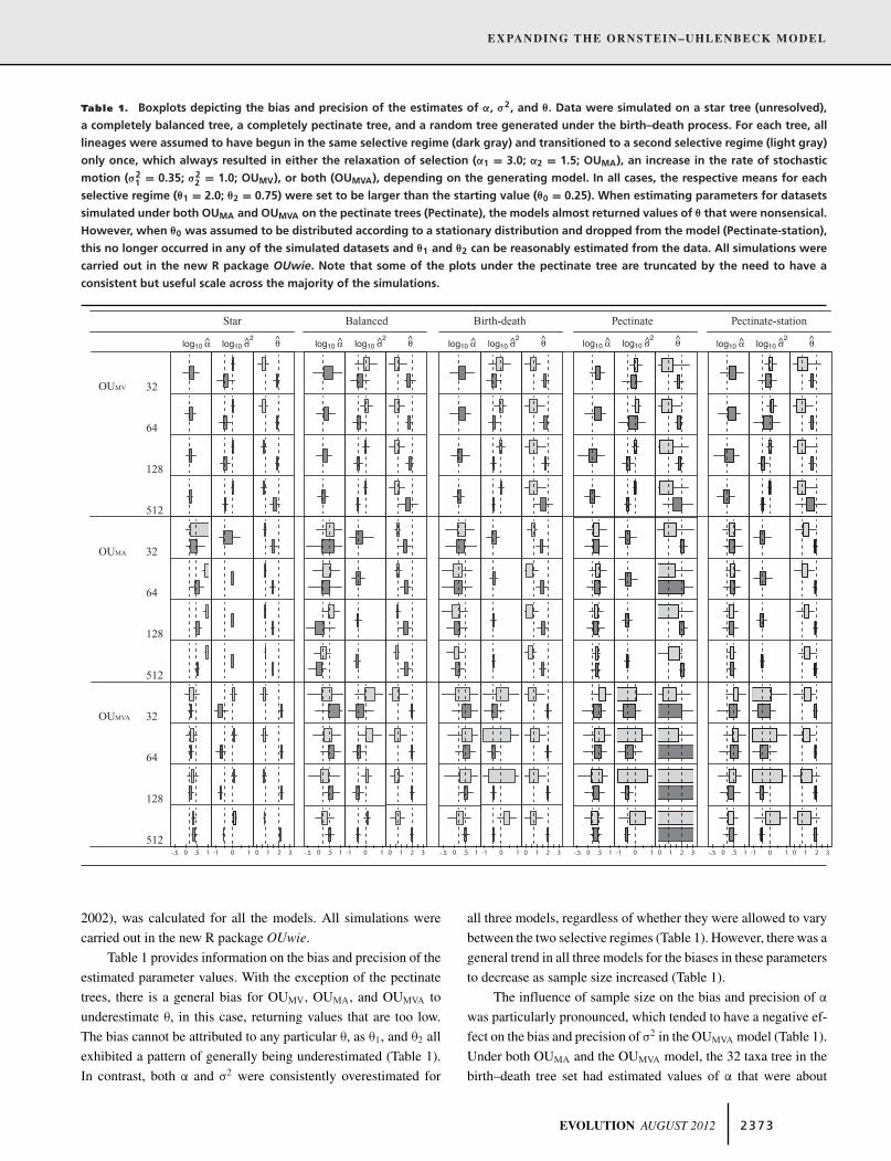
Table 1. Boxplots depicting the bias and precision of the estimates of ", #2, and !. Data were simulated on a star tree (unresolved),a completely balanced tree, a completely pectinate tree, and a random tree generated under the birth–death process. For each tree, alllineages were assumed to have begun in the same selective regime (dark gray) and transitioned to a second selective regime (light gray)only once, which always resulted in either the relaxation of selection ("1 = 3.0; "2 = 1.5; OUMA), an increase in the rate of stochasticmotion (#2

1 = 0.35; #22 = 1.0; OUMV), or both (OUMVA), depending on the generating model. In all cases, the respective means for each

selective regime (!1 = 2.0; !2 = 0.75) were set to be larger than the starting value (!0 = 0.25). When estimating parameters for datasetssimulated under both OUMA and OUMVA on the pectinate trees (Pectinate), the models almost returned values of ! that were nonsensical.However, when !0 was assumed to be distributed according to a stationary distribution and dropped from the model (Pectinate-station),this no longer occurred in any of the simulated datasets and !1 and !2 can be reasonably estimated from the data. All simulations werecarried out in the new R package OUwie. Note that some of the plots under the pectinate tree are truncated by the need to have aconsistent but useful scale across the majority of the simulations.

OUMV

OUMA

OUMVA

32

64

128

512

32

64

128

512

32

64

128

512

BalancedStar Birth-death Pectinate

l !og10 " log10 #2

l !og10 " log10 #2

l !og10 " log10 #2

l !og10 " log10 #2

Pectinate-station

l !og10 " log10 #2

-.5 0 .5 1 -1 0 1 0 1 2 3 -.5 0 .5 1 -1 0 1 0 1 2 3 -.5 0 .5 1 -1 0 1 0 1 2 3 -.5 0 .5 1 -1 0 1 0 1 2 3 -.5 0 .5 1 -1 0 1 0 1 2 3

2002), was calculated for all the models. All simulations werecarried out in the new R package OUwie.

Table 1 provides information on the bias and precision of theestimated parameter values. With the exception of the pectinatetrees, there is a general bias for OUMV, OUMA, and OUMVA tounderestimate $, in this case, returning values that are too low.The bias cannot be attributed to any particular $, as $1, and $2 allexhibited a pattern of generally being underestimated (Table 1).In contrast, both ! and #2 were consistently overestimated for

all three models, regardless of whether they were allowed to varybetween the two selective regimes (Table 1). However, there was ageneral trend in all three models for the biases in these parametersto decrease as sample size increased (Table 1).

The influence of sample size on the bias and precision of !

was particularly pronounced, which tended to have a negative ef-fect on the bias and precision of #2 in the OUMVA model (Table 1).Under both OUMA and the OUMVA model, the 32 taxa tree in thebirth–death tree set had estimated values of ! that were about



twice, on average, the true values (Table 1). The bias dropped assample size increased, but even with a tree of 512 taxa the biaswas never less than 1.10 times the true value. However, whensimulating datasets under the OUM model (results not shown),the bias with a 512 taxa tree was larger and exceeded 1.25 timesthe true value. A key question for many empiricists using thesemethods is not “what is the value of ! in each regime” but “is thevalue of ! in Regime 1 much bigger than the value in Regime 2.”Looking at cases where the model returned an ! for Regime 1 thatwas at least 10% higher than the ! returned for Regime 2, roughly19% of the datasets simulated on the 512 taxa tree were belowthis threshold (with only 12% of all datasets inferring a higher !

for Regime 2). However, for the 128 taxa tree, nearly 50% of thesimulated datasets returned an ! for Regime 1 that was less than10% higher than ! for Regime 2. Taken together, these resultssuggest that even for moderately sized datasets (e.g., (150 taxa)it may be difficult to confidently infer meaningful differences in !

among selective regimes. The model parameters for these datasetswill tend to return larger values of ! with greater uncertainty.

In the pectinate trees, when simulating datasets under bothOUMA and OUMVA, the models returned values of $ that werenonsensical. Interestingly, when we reran the simulations acrossthe pectinate trees with $0 dropped from the model, this behav-ior no longer occurred in any of the simulated datasets (Table 1).Dropping $0 from the model assumes that the starting value is dis-tributed according to the stationary distribution of the OU process,where the conditional distribution of X(T) given X(0) in equation(8) are assumed to have converged on the same distribution. Thiswould not fit a biological scenario involving a trend away from anancestral state, but it does fit a scenario of a stationary evolution-ary process: the same distribution of optima, selection, and ratesoccur in the past as in the present. Under this assumption, the gen-eral bias was for OUMA and OUMVA to overestimate $ associatedwith Regime 2 (Table 1). This suggests caution when compar-ing values of $ among selective regimes when the tree is highlyimbalanced—they will tend to be unreliable or, at least, very im-precise and associated with very large standard errors. In suchinstances, it may be helpful to drop $0 from the model entirely.

We note that under some circumstances it may be impossibleto estimate $0 accurately. Under the OU process the influenceof the starting state, $0, on the expected values exponentiallydecreases at a rate that is determined by !. For larger values of !,a trait is generally free from the constraints of the starting stateand will be much closer to the optimal value for the selectiveregime it is currently in. As a result, the weighting factor in Wrepresenting the influence of the root will decrease and estimatesof $0 should approach zero. Thus, for large values of ! (i.e., !

> 2), the estimates of $0 will always be small, and the standarderror surrounding $0 is likely to be positively misleading (i.e.,false precision).

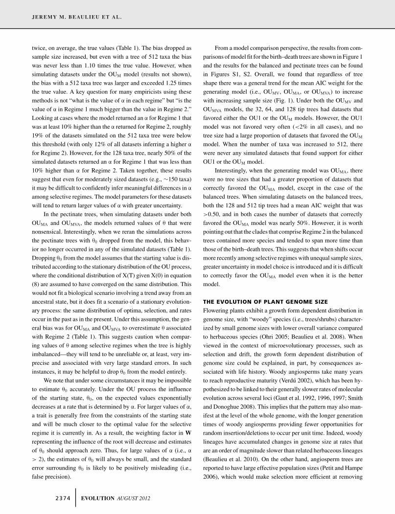
From a model comparison perspective, the results from com-parisons of model fit for the birth–death trees are shown in Figure 1and the results for the balanced and pectinate trees can be foundin Figures S1, S2. Overall, we found that regardless of treeshape there was a general trend for the mean AIC weight for thegenerating model (i.e., OUMV, OUMA, or OUMVA) to increasewith increasing sample size (Fig. 1). Under both the OUMV andOUMVA models, the 32, 64, and 128 tip trees had datasets thatfavored either the OU1 or the OUM models. However, the OU1model was not favored very often (<2% in all cases), and notree size had a large proportion of datasets that favored the OUM

model. When the number of taxa was increased to 512, therewere never any simulated datasets that found support for eitherOU1 or the OUM model.

Interestingly, when the generating model was OUMA, therewere no tree sizes that had a greater proportion of datasets thatcorrectly favored the OUMA model, except in the case of thebalanced trees. When simulating datasets on the balanced trees,both the 128 and 512 tip trees had a mean AIC weight that was>0.50, and in both cases the number of datasets that correctlyfavored the OUMA model was nearly 50%. However, it is worthpointing out that the clades that comprise Regime 2 in the balancedtrees contained more species and tended to span more time thanthose of the birth–death trees. This suggests that when shifts occurmore recently among selective regimes with unequal sample sizes,greater uncertainty in model choice is introduced and it is difficultto correctly favor the OUMA model even when it is the bettermodel.

THE EVOLUTION OF PLANT GENOME SIZE

Flowering plants exhibit a growth form dependent distribution ingenome size, with “woody” species (i.e., trees/shrubs) character-ized by small genome sizes with lower overall variance comparedto herbaceous species (Ohri 2005; Beaulieu et al. 2008). Whenviewed in the context of microevolutionary processes, such asselection and drift, the growth form dependent distribution ofgenome size could be explained, in part, by consequences as-sociated with life history. Woody angiosperms take many yearsto reach reproductive maturity (Verdu 2002), which has been hy-pothesized to be linked to their generally slower rates of molecularevolution across several loci (Gaut et al. 1992, 1996, 1997; Smithand Donoghue 2008). This implies that the pattern may also man-ifest at the level of the whole genome, with the longer generationtimes of woody angiosperms providing fewer opportunities forrandom insertion/deletions to occur per unit time. Indeed, woodylineages have accumulated changes in genome size at rates thatare an order of magnitude slower than related herbaceous lineages(Beaulieu et al. 2010). On the other hand, angiosperm trees arereported to have large effective population sizes (Petit and Hampe2006), which would make selection more efficient at removing



Number of taxa

AIC

wei

ght (

wi)

0.0

0.2

0.4

0.6

0.8

1.0

32 64 128 512

Number of taxa

AIC

wei

ght (

wi)

0.0

0.2

0.4

0.6

0.8

1.0

32 64 128 512

Number of taxa

AIC

wei

ght (

wi)

0.0

0.2

0.4

0.6

0.8

1.0

32 64 128 512

A B

C

Figure 1. Comparisons of model fit based on AIC weights (wi) for birth–death trees comprised of 32, 64, 128, and 512 taxa. Data weresimulated under each of the three OU models that allowed the rate of stochastic motion (#2) to vary (OUMV, A), or the strength ofselection (") to vary (OUMA, B), for both to vary (OUMVA, C). When their fit (·) was compared against a simple OU model that assumed asingle optimum for all species (OU1, !) and an OU model that assumed different state means and a single " and #2 acting all selectiveregimes (OUM, I), there was a general trend for the mean AIC weight to increase with increasing sample size.

deleterious mutations and excess DNA (Lynch 2007). Strongerselection in woody species would also be consistent with thesuggestion that large increases in DNA content negatively affectwoody growth and physiology (Stebbins 1938; Beaulieu et al.2008). Here, we illustrate our method by testing for an asymme-try in the strength of selection and stochastic motion acting ongenome size due to growth form.

We focus our analysis on the Monocotyledonae (monocots;Cantino et al. 2007), a major branch of the angiosperms. Themonocots are a large clade of mainly herbaceous angiospermsthat also contain a few clades of predominately woody species, in-cluding the palms (Arecales; APG III 2009). However, it is worthnoting that unlike other woody angiosperms, “woody” monocotsdo not produce true “wood” (i.e., secondary xylem). Here, we gen-erally define the tree/shrub or “woody” category as simply largeplants with long generation times (e.g., Smith and Donoghue

2008). Genome size estimates were taken from the Plant DNAC-values database (release 5.0; Bennett and Leitch 2010) formonocot species where both the 1C amount (the amount of DNAin the unreplicated gametic nucleus) and the ploidy level wereknown. Genome size was log10-transformed prior to all analy-ses to ensure the data minimally conformed to Brownian motionevolution (O’Meara et al. 2006; Oliver et al. 2007).

The procedure used to construct a large sequence based phy-logeny follow the methods described by Smith et al. (2009) andimplemented in the program PHLAWD. We specified atpB, matK,ndhF, rbcL, and trnL-F as our genes of interest and we limitedour search of GenBank to only return sequences for taxa repre-sented in our genome size dataset. Our final combined sequencematrix contained 590 species and 7213 aligned sites. We con-ducted 100 maximum likelihood analyses on this matrix usingthe standard RAxML search algorithm under the GTR+CAT



approximation of rate heterogeneity partitioned for each gene(Stamatakis 2006). The final 100 topologies were rooted withAcorales (sensu Chase et al. 2006) and scored under GTR+! toestimate molecular branch lengths and to identify the tree withhighest likelihood score. We assigned minimum age constraintsbased on 14 described fossils with unequivocal affinities to cladesnested within the monocots (see Supporting Information). Themaximum-likelihood (ML) tree was then converted to ultrametricusing the semiparametric penalized likelihood method developedby Sanderson (2003) and implemented in r8s. The cross-validationprocedure was used to find the optimal value of the smoothing pa-rameter ()). To accommodate our large tree, we randomly prunedour ML tree to 60 taxa 10 times, and the consistent best esti-mate of ) was used to smooth the rates across the entire ML tree.The final tree is available at TreeBASE (http://www.treebase.org),accession number 12409.

Slow growing, tall, and “woody” genera have beendescribed in several different monocot families, includingArecaceae, Asparagaceae (e.g., Dasylirion, Dracaena, Nolina,Xanthorrhoea), Bromeliaceae (e.g., Puya), Dasypogonaceae(Dasypogon, Kingia), Pandanaceae (Pandanus), Strelitziaceae(e.g., Ravenala), and the woody bamboo genera in the tribeBambuseae of Poaceae (e.g., Phyllostachys, Semiarundinaria,Sasa). However, due to the absence of genome size and/orsequence data for many of these genera the effect of growth formanalyses were restricted to comparisons between (1) Dasypogon(Dasypogonaceae; 1 species) and the “woody” palms (Arecaceae;36 species), and (2) the remaining species that were scored asherbaceous (553 species). We reconstructed the likeliest growthform at all internal nodes of our dated ML tree using a likelihood-based ancestral state reconstruction model (Pagel 1999) thatassumed equal transitions rates between character states. Giventhese internal estimates, the simplest explanation is a singletransition from herbaceous to the woody habit reconstructedalong the branch leading to the split between Dasypogon and theArecales (Fig. 2A).

We fit six different models of genome size evolution. Thetwo simplest models were a single-rate Brownian motion model(BM1) and an OU model with one optimum for all species ofmonocots (OU1). We fit a multiple rate Brownian motion modelthat assigned a separate rate for each character state (BMRC). Inthis case, a separate rate was assigned to woody and herbaceouslineages. The OUM model assumed two optima for each growthform while keeping both ! and #2 constant. Finally, we assessedthe fit of the OUMV, OUMA, and OUMVA models that assumedtwo optima but varied ! and #2 between woody and herbaceouslineages. In all cases, we dropped $0 from the model and assumedthat the starting value was distributed according to the stationarydistribution of the OU process (see above). All tests were carriedout in OUwie using the “noncensored” approach of O’Meara

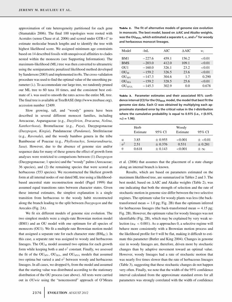
Table 2. The fit of alternative models of genome size evolutionin monocots. The best model, based on $AIC and Akaike weights,was the OUMVA, which estimated a separate !, ", and #2 for woodyand herbaceous monocot lineages.

Model -lnL AIC "AIC wi

BM1 "227.6 459.1 156.2 <0.01BMS "203.0 412.0 109.1 <0.01OU1 "160.0 326.1 23.2 <0.01OUM "159.2 326.5 23.6 <0.01OUMV "147.3 304.6 1.7 0.290OUMA "159.2 328.5 25.6 <0.01OUMVA "145.3 302.9 0.0 0.678

Table 3. Parameter estimates and their associated 95% confi-dence interval (CI) for the OUMVA model, the model that best fit thegenome size data. Each CI was obtained by multiplying each ap-proximate standard error by the critical value in the t-distributionwhere the cumulative probability is equal to 0.975 (i.e., t (0.975,!) = 1.96).

Herb WoodyEstimate 95% CI Estimate 95% CI

! 3.85 ± 0.955 <0.001 ± <0.01#2 2.51 ± 0.376 0.531 ± 0.281$ 0.618 ± 0.143 <0.001 ± '

et al. (2006) that assumes that the placement of a state changealong an internal branch is known.

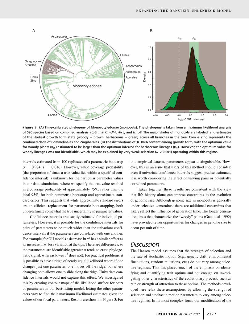
Results, which are based on parameters estimated on themaximum likelihood tree, are summarized in Tables 2 and 3. Thebest model, based on "AIC and Akaike weights (Table 2), wasone indicating that both the strength of selection and the rate ofstochastic motion in genome size differ between the two selectiveregimes. The optimum value for woody plants was less (the back-transformed mean = 1.0 pg; Fig. 2B) than the optimum inferredfor herbaceous lineages (the back-transformed mean = 4.15 pg;Fig. 2B). However, the optimum value for woody lineages was notidentifiable (Fig. 2B), which may be explained by very weak se-lection (!W < 0.001). As ! approaches 0, a selective regime willbehave more consistently with a Brownian motion process andthe likelihood profile for $ will be flat, making it difficult to esti-mate this parameter (Butler and King 2004). Changes in genomesize in woody lineages are, therefore, driven more by stochasticchanges than by adaptive movement toward an optimal value.However, woody lineages had a rate of stochastic motion thatwas nearly five times slower than the rate of herbaceous lineages(Table 3), suggesting that these stochastic changes do not happenvery often. Finally, we note that the width of the 95% confidenceinterval calculated from the approximate standard errors for allparameters was strongly correlated with the width of confidence



Figure 2. (A) Time-calibrated phylogeny of Monocotyledonae (monocots). The phylogeny is taken from a maximum likelihood analysisof 590 species based on combined analysis atpB, matK, ndhF, rbcL, and trnL-F. The major clades of monocots are labeled, and estimatesof the likeliest growth form state (woody = brown; herbaceous = green) across all branches in the tree. Com + Zing represents thecombined clade of Commelinales and Zingiberales. (B) The distributions of 1C DNA content among growth form, with the optimum valuefor woody plants (!W) estimated to be larger than the optimum inferred for herbaceous lineages (!H). However, the optimum value forwoody lineages was not identifiable, which may be explained by very weak selection (" < 0.001) operating within this regime.

intervals estimated from 100 replicates of a parametric bootstrap(r = 0.984, P = 0.016). However, while coverage probability(the proportion of times a true value lies within a specified con-fidence interval) is unknown for the particular parameter valuesin our data, simulations where we specify the true value resultedin a coverage probability of approximately 75%, rather than theideal 95%, for both parametric bootstrap and approximate stan-dard errors. This suggests that while approximate standard errorsare an efficient replacement for parametric bootstrapping, bothunderestimate somewhat the true uncertainty in parameter values.

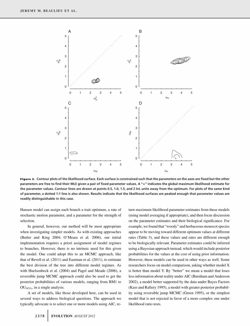
Confidence intervals are usually estimated for individual pa-rameters. However, it is possible for the confidence intervals forpairs of parameters to be much wider than the univariate confi-dence intervals if the parameters are correlated with one another.For example, for OU models a decrease in #2 has a similar effect asan increase in !: less variation at the tips. There are differences, sothe parameters are identifiable (greater ! tends to erase phyloge-netic signal, whereas lower #2 does not). For practical problems, itis possible to have a ridge of nearly equal likelihood where if onechanges just one parameter, one moves off the ridge, but wherechanging both allows one to slide along the ridge. Univariate con-fidence intervals would not capture this effect. We investigatedthis by creating contour maps of the likelihood surface for pairsof parameters in our best-fitting model, letting the other param-eters vary to find their maximum likelihood estimates given thevalues of our focal parameters. Results are shown in Figure 3. For

this empirical dataset, parameters appear distinguishable. How-ever, this is an issue that users of this method should consider:even if univariate confidence intervals suggest precise estimates,it is worth considering the effect of varying pairs or potentiallycorrelated parameters.

Taken together, these results are consistent with the viewthat life history alone can impose constraints to the evolutionof genome size. Although genome size in monocots is generallyunder selective constraints, there are additional constraints thatlikely reflect the influence of generation time. The longer genera-tion times that characterize the “woody” palms (Gaut et al. 1992)have provided fewer opportunities for changes in genome size tooccur per unit of time.

DiscussionThe Hansen model assumes that the strength of selection andthe rate of stochastic motion (e.g., genetic drift, environmentalfluctuations, random mutations, etc.) do not vary among selec-tive regimes. This has placed much of the emphasis on identi-fying and quantifying trait optima and not enough on investi-gating other characteristics of the evolutionary process, such asrate or strength of attraction to these optima. The methods devel-oped here relax these assumptions, by allowing the strength ofselection and stochastic motion parameters to vary among selec-tive regimes. In its most complex form, our modification of the



0

1

2

3

4

5

0 1 2 3 4 5

+

0

1

2

3

4

5

0 1 2 3 4 5

+

0

1

2

3

4

5

0 1 2 3 4 5

+

0

1

2

3

4

5

0 1 2 3 4 5

+

#H2

# W2

A

"W

# W2

C

# H2

B

"H

D

" W

"H

Figure 3. Contour plots of the likelihood surface. Each surface is constrained such that the parameters on the axes are fixed but the otherparameters are free to find their MLE given a pair of fixed parameter values. A “+” indicates the global maximum likelihood estimate forthe parameter values. Contour lines are drawn at points 0.5, 1.0, 1.5, and 2 lnL units away from the optimum. For plots of the same kindof parameter, a dotted 1:1 line is also shown. Results indicate that the likelihood surfaces are peaked enough that parameter values arereadily distinguishable in this case.

Hansen model can assign each branch a trait optimum, a rate ofstochastic motion parameter, and a parameter for the strength ofselection.

In general, however, our method will be most appropriatewhen investigating simpler models. As with existing approaches(Butler and King 2004; O’Meara et al. 2006), our initialimplementation requires a priori assignment of model regimesto branches. However, there is no intrinsic need for this giventhe model. One could adopt this to an MCMC approach, likethat of Revell et al. (2011) and Eastman et al. (2011), to estimatethe best division of the tree into different model regimes. Aswith Huelsenbeck et al. (2004) and Pagel and Meade (2006), areversible jump MCMC approach could also be used to get theposterior probabilities of various models, ranging from BM1 toOUMVA, in a single analysis.

A set of models, like those developed here, can be used inseveral ways to address biological questions. The approach wetypically advocate is to select one or more models using AIC, re-

turn maximum likelihood parameter estimates from these models(using model averaging if appropriate), and then focus discussionon the parameter estimates and their biological significance. Forexample, we found that “woody” and herbaceous monocot speciesappear to be moving toward different optimum values at differentrates (Table 3), and these values and rates are different enoughto be biologically relevant. Parameter estimates could be inferredusing a Bayesian approach instead, which would include posteriorprobabilities for the values at the cost of using prior information.However, these models can be used in other ways as well. Someresearchers focus on model comparison, asking whether model Xis better than model Y. By “better” we mean a model that losesless information about reality under AIC (Burnham and Anderson2002), a model better supported by the data under Bayes Factors(Kass and Raftery 1995), a model with greater posterior probabil-ity using reversible jump MCMC (Green 1995), or the simplestmodel that is not rejected in favor of a more complex one underlikelihood ratio tests.



As biologists, we find the exercise of being primarily con-cerned about which model is best rather than about what theparameter estimates are under the best model(s), less compelling.Biological reality is undoubtedly more complex, especially acrossmany species, than any single evolutionary model we may ex-amine. Fit of a model, especially when compared with a morecomplex model, is based on both how well the model param-eters match the generating processes in the real world but alsohow much data are available to use in fitting. A model for hu-man height where the dependent variable of offspring height isrelated to maternal height is probably a better fit to the data thana model that relates day of the week of birth for good biologicalreasons. A model incorporating maternal height, maternal nutri-tion, offspring nutrition, history of offspring disease, and the fullgenomic sequence of the offspring will undoubtedly be a betterfit than either model, but only once there are enough height data.We would rather investigate, say, the magnitude of the heritableeffect of maternal height on offspring height rather than whetheroffspring disease history is included or excluded from the bestmodel. In any case, there are many ways to do good science, andwe have endeavored in this article to evaluate how well these newmethods will perform in whatever framework they are used in,whether parameter estimation or model comparison.

We have described the models here as reflecting drift, se-lection, and other evolutionary processes. However, we note acommon misunderstanding with this sort of model: although theoverall parameters resemble those of microevolutionary models(for example, for selection) they are actually describing the pat-tern of evolutionary change. As shown by Hansen and Martins(1996), even a simple model like single rate Brownian motionis consistent with neutral genetic drift, selection toward a mov-ing optimum, drift-mutation balance, and other evolutionary pro-cesses. Thus, one can investigate whether parameter estimates areconsistent with predictions (i.e., a hypothesis that after a massextinction, the rate of evolution is increased due to diminishedpopulation sizes and more drift), but it is difficult to work theother way and use information about the best model or parameterestimates to draw conclusions about evolutionary processes.

In regards to parameter estimation, our simulations suggestthat accurate parameter estimates will often require larger samplesizes, especially when the underlying hypothesis involves testingfor differences in the strength of selection. The issue of samplesize need not only apply to the total size of a given tree. Accurateparameter estimates may be difficult even for a large tree if itis divided up among many selective regimes each comprised ofrelatively few species and branches. That is not to say that ourmethods should not be applied to smaller datasets or selectiveregimes comprised of few species. We only advise that conclu-sions be made cautiously. As our simulations suggest, there willbe circumstances in which meaningful patterns can be extracted

from smaller sample sizes. These will be instances where the sig-nal in the data is particularly strong. However, one should bearin mind that parameter estimates (especially for !) are generallyoverestimated with smaller datasets (i.e., <128 species). In thisregard, it will be prudent to interpret results in light of the standarderror or confidence interval associated with each of the param-eters. At times, it may be more meaningful to make qualitativestatements about parameter differences.

It would appear then that the models described here will nat-urally compliment the very large, comprehensive trees that arecurrently being generated by mining data from DNA sequencerepositories (e.g., McMahon and Sanderson 2006; Sandersonet al. 2008; Smith et al. 2009, 2011; Thomson and Shaffer 2010).Applying our methods to these large datasets hold the promiseof greater insights into evolution across broader phylogenetic andtemporal scales and can point to a number of patterns that couldnot previously have been recognized and quantified. The methodsdescribed here can begin to address important comparative ques-tions and hypotheses underlying major morphological radiationsacross the tree of life. For example, is the immense morphologicaldiversity observed within flowering plants consistent with higherrates of evolution due to their generally faster generation times(Stebbins 1981; Bond 1989)? Is the low morphological diversityobserved within marsupials related to constraints posed by theirmode of reproduction (Lillegraven 1975; Sears 2004)? Do bio-geographic movements result in tracking ancestral optima or theevolution of new climatic tolerances (Donoghue 2008)? We be-lieve that studies along these lines will open up new avenues ofresearch.

PROGRAM NOTE

The methods and simulations described above are implementedin the R package OUwie (pronounced “au-wi”), available throughCRAN. We have also made OUwie available in the Discov-ery Environment at http://preview.iplantcollaborative.org. TheDiscovery Environment is a web-based integrated plat-form for data exploration and scientific discovery http://www.iplantcollaborative.org/discover/discovery-environment.

As input OUwie requires a phylogeny with branch lengthsand internal node labels denoting the selective regimes at ancestralnodes, and a trait file that contains information for each speciesregarding the current selective regime and the values of a quanti-tative trait. The user can specify a series of models ranging fromthose based on Brownian motion processes available in Brownie(O’Meara et al. 2006), to the OU models available in Butler andKing’s (2004) program ouch and the ones described here. OUwieuses a bounded subplex routine for minimizing the likelihoodfunction to find the optimal parameter estimates. The user is alsoprovided a series of model diagnostics indicating whether the like-lihood search returned stable and reliable parameter estimates.



ACKNOWLEDGMENTSThanks are due to Jason Shapiro, Alex Dornburg, Jeff Oliver, Beth For-restel, Barb Banbury, and Matt Pennell for useful feedback on the methodimplementation and for helpful suggestions on the manuscript. Supportfor JMB and BCO has been provided by the iPTOL program within theNSF-funded iPlant Collaborative (http://www.iplantcollaborative.org/).Support for DCJ has been provided by the National Institute for Mathe-matical and Biological Synthesis, an Institute sponsored by the NationalScience Foundation, the U.S. Department of Homeland Security, and theU.S. Department of Agriculture through NSF Award #EF-0832858, withadditional support from The University of Tennessee, Knoxville.

LITERATURE CITEDAkaike, H. 1974. A new look at the statistical model identification. IEEE

Trans. Automat. Contr. 19:716–723.Angiosperm Phylogeny Group. 2009. An update of the Angiosperm Phy-

logeny Group classification for the orders and families of floweringplants: APG III. Bot. J. Linn. Soc. 161:105–121.

Beaulieu, J. M., I. J. Leitch, S. Patel, A. Pendharkar, and C. A. Knight. 2008.Genome size is a strong predictor of cell size and stomatal density inangiosperms. New Phytol. 179:975–986.

Beaulieu, J. M., S. A. Smith, and I. J. Leitch. 2010. On the tempo of genomesize evolution in angiosperms. J. Bot. doi:10.1155/2010/989152

Bennett, M. D., and I. J. Leitch. 2010. Plant DNA C-values database (release5.0, Dec. 2010). Available at http://kew.org/genomesize/homepage

Bond, W. J. 1989. The tortoise and the hare: ecology of angiospermdominance and gymnosperm persistence. Biol. J. Linn. Soc. 36:227–249.

Burnham, K. P., and D. R. Anderson. 2002. Model selection and multimodel in-ference: a practical information-theoretic approach. New York, Springer-Verlag.

Butler, M. A., and A. A. King. 2004. Phylogenetic comparative analy-sis: a modeling approach for adaptive evolution. Am. Nat. 164:683–695.

Cantino, P. D., J. A. Doyle, S. W. Graham, W. S. Judd, R. G. Olmstead, D. E.Soltis, P. S. Soltis, and M. J. Donoghue. 2007. Towards a phylogeneticnomenclature of Tracheophyta. Taxon 56:822–846.

Chase, M. W., M. F. Fay, D. S. Devey, O. Maurin, N. Rønsted, T. J. Davies,Y. Pillon, G. Petersen, O. Seberg, M. N. Tamura, et al. 2006. Multigeneanalyses of monocot relationships: a summary. Aliso 22:63–75.

Collar, D. C., B. C. O’Meara, P. C. Wainwright, and T. J. Near. 2009. Pis-civory limits diversification of feeding morphology in centrarchid fishes.Evolution 63:1557–1573.

Davis, C. C., M. Latvis, D. L. Nickrent, K. J. Wurdack, and D. A. Baum. 2007.Floral gigantism in Rafflesiaceae. Science 315:1812.

Donoghue, M. J. 2008. A phylogenetic perspective on the distribution of plantspecies. Proc. Natl. Acad. Sci. USA 105:11549–11555.

Eastman, J. M., M. E. Alfaro, P. Joyce, A. L. Hipp, and L. J. Har-mon. 2011. AUTEUR: a novel comparative method for modelingshifts in the rate of character evolution on trees. Evolution: 65:3578–3589.

Edwards, E. J., and S. A. Smith. 2010. Phylogenetic analyses reveal the shadyhistory of C4 grasses. Proc. Natl. Acad. Sci. USA 6:2532–2537.

Gaut, B. S., S. V. Muse, W. D. Clark, and M. T. Clegg. 1992. Relative rates ofnucleotide substitution at the rbcL locus of monocotyledonous plants. J.Mol. Evol. 35:292–303.

Gaut, B. S., B. R. Morton, B. C. McCraig, and M. T. Clegg. 1996. Substitutionrate comparisons between grasses and palms: synonymous rate differ-ences at the nuclear gene Adh parallel rate differences at the plastid generbcL. Proc. Natl. Acad. Sci. USA 93:10274–10279.

Gaut, B. S., L. G. Clark, J. F. Wendel, and S. V. Muse. 1997. Comparisons ofthe molecular evolutionary process at rbcL and ndhF in the grass family(Poaceae). Mol. Biol. Evol. 14:769–777.

Green, P. J. 1995. Reversible jump Markov chain monte carlo com-putation and Bayesian model determination. Biometrika 82:711–732.

Hansen, T. F. 1997. Stabilizing selection and the comparative analysis ofadaptation. Evolution 51:1341–1351.

Hansen, T. F., and E. P. Martins. 1996. Translating between microevolution-ary process and macroevolutionary patterns: the correlation structure ofinterspecific data. Evolution 50:1404–1417.

Harmon, L. J., J. Melville, A. Larson, and J. B. Losos. 2008. The role of ge-ography and ecological opportunity in the diversification of day geckos(Phelsuma). Syst. Biol. 57:562–573.

Harmon, L. J., J. B. Losos, T. J. Davies, R. G. Gillespie, J. L. Gittleman, W.B. Jennings, K. H. Kozak, M. A. McPeek, F. Moreno-Roark, T. J. Near,et al. 2010. Early bursts of body size and shape evolution are rare incomparative data. Evolution 64:2385–2396.

Huelsenbeck, J. P., B. Larget, and M. E. Alfaro. 2004. Bayesian phylogeneticmodel selection using reversible jump Markov Chain Monte Carlo. Mol.Biol. Evol. 21:1123–1133.

Kass, R. E., and A. E. Raftery. 1995. Bayes factors. J. Am. Stat. Assoc.90:773–795.

Lillegraven, J. A. 1975. Biological considerations of the marsupial-placentaaldichotomy. Evolution 29:707–722.

Lynch, M. 2007. The origins of genome architecture. Sinauer Assocs., Inc.,Sunderland.

McMahon, M. M., and M. J. Sanderson. 2006. Phylogenetic supermatrixanalysis of GenBank sequences from 2228 papilionoid legumes. Syst.Biol. 55:818–836.

Oliver, M. J., D. Petrov, D. D. Ackerly, P. Falkowski, and O. M. Schofield.2007. The mode and tempo of genome size evolution in eukaryotes.Genome Res. 17:594–601.

O’Meara, B. C., C. Ane, M. J. Sanderson, and P. C. Wainwright. 2006.Testing for different rates of continuous trait evolution. Evolution 60:922–933.

Ohri, D. 2005. Climate and growth form: the consequences for genome sizein plants. Plant Biol. 7:449–458.

Pagel, M. 1999. The maximum likelihood approach to reconstructing ances-tral character states of discrete characters on phylogenies. Syst. Biol.48:612–622.

Pagel, M., and A. Meade. 2006. Bayesian analysis of correlated evolution ofdiscrete characters by reversible-jump Markov Chain Monte Carlo. Am.Nat. 167:808–825.

Petit, R. J., and A. Hampe. 2006. Some evolutionary consequences of being atree. Annu. Rev. Ecol. Evol. Syst. 37:187–214.

Pinto, G., D. L. Mahler, L. J. Harmon, and J. B. Losos. 2008. Testing theisland effect in adaptive radiation: rates and patterns of morphologicaldiversification in Caribbean and mainland Anolis lizards. Proc. R. Soc.B 275:2749–2757.

Revell, L. J., L. D. Mahler, P. R. Peres-Neto, and B. D. Redelings. 2011. Anew phylogenetic method for identifying exceptional phenotypic diver-sification. Evolution: 66:135–146.

Sanderson, M. J. 2003. r8s: inferring absolute rates of molecular evolution anddivergence times in the absence of a molecular clock. Bioinformatics19:301–302.

Sanderson, M. J., D. Boss, D. Chen, K. A. Cranston, and A. Wehe. 2008. ThePhyLoTA browser: processing GenBank for molecular phylogeneticsresearch. Syst. Biol. 57:335–346.

Sears, K. E. 2004. Constraints on the morphological evolution of marsupialshoulder girdles. Evolution 58:2353–2370.



Smith, S. A., and J. M. Beaulieu. 2009. Life history influences rates of climaticniche evolution in flowering plants. Proc. R. Soc. Lond. B 276:4345–4352.

Smith, S. A., and M. J. Donoghue. 2008. Rates of molecular evolu-tion are linked to life history in flowering plants. Science 322:86–89.

Smith, S. A., J. M. Beaulieu, and M. J. Donoghue. 2009. Mega-phylogenyapproach for comparative biology: an alternative to supertree and super-matrix approaches. BMC Evol. Biol. 9:1–12.

Smith, S. A., J. M. Beaulieu, A. Stamatakis, and M. J. Donoghue. 2011. Under-standing angiosperm diversification using small and large phylogenetictrees. Am. J. Bot. 98:1–12.

Stamatakis, A. 2006. Maximum likelihood-based phylogenetic analyseswith thousands of taxa and mixed models. Bioinformatics 22:2688–2690.

Stebbins, G. L. 1938. Cytological characteristics associated with differentgrowth habits in dicotyledons. Am. J. Bot. 25:189–198.

———. 1981. Why are there so many species of flowering plants? Bioscience31:573–577.

Thomas, G. H., R. P. Freckleton, and T. Szekely. 2006. Comparativeanalyses of the influence of developmental mode on phenotypic di-versification rates in shorebirds. Proc. R. Soc. Lond. B 273:1619–1624.

Thomson, R. C., and H. B. Shaffer. 2010. Sparse supermatrices for phyloge-netic inference: taxonomy, alignment, rogue taxa, and the phylogeny ofliving turtles. Syst. Biol. 59:42–58.

Verdu, M. 2002. Age at maturity and diversification in woody angiosperms.Evolution 56:1352–1361.

Associate Editor: L. Kubatko

AppendixThe Generalized Hansen ModelLet Xi (t) be the trait at time t. We assume that Xi (t) satisfies thesolution of the stochastic differential equation

d Xi (t) = !i (t)("i (t) " Xi (t))dt + #i (t)d B(t),

where d B(t) denotes the white noise process, !i (t) measures therate of adaption, "i (t)is the primary optimum of Xi , and #i (t)measures size of stochastic perturbation at time t.

Multiplying both sides by the integral factor e( t

0 !i (s)ds andapplying the chain rule and the fundamental theorem of calculusyields the differential equation

dXi (t)e( t

0 !i (s)ds = !i (t)"i (t)e( t

0 !i (s)dsdt + #i (t)e( t

0 !i (s)dsdBi (t).

Given the initial condition Xi (0) = $0, the solution to thisequation is

Xi (t) =)! t

0!i (s)"i (s)e

( s0 !i (x)dx ds

*e"

( t0 !i (s)ds

+)! t

0#i (s)e

( s0 !i (x)dx dB(s)

*e"

( t0 !i (s)ds + $0e"

( t0 !i (s)ds .

Because this defines a Gaussian process, the first moment ofXi (t) is completely specified. In particular, we have

E#Xi (T )|Xi (0) = $0

$= $0e"

( T0 !i (t)dt

+e"( T

0 !i (t)dt8( T

0 !i (t)"i (t)e( t

0 !i (x)dx dt9

,

and the covariation between species i and species j is

Cov[Xi (T ), X j (T )|Xi (0) = X j (0) = $0]= E[Xi (T ) · X j (T )|Xi (0) = X j (0) = $0]

"E[Xi (T )|Xi (0) = $0]E[X j (T )|X j (0) = $0].

= E((e"( T

0 !i (t)+! j (t)dt )8( T

0 #i (t)e( t

0 !i (x)dx dBi (t)9

#8( T

0 # j (t)e( t

0 ! j (x)dx dB j (t))9

.

COVARIANCE STRUCTURE

The differential equation defining the covariation between speciesi and j assumes that both !i and #i are a function of time. How-ever, this equation also includes the much simpler cases suchas when neither is allowed to vary (OUM), or when only #i

is allowed to vary (OUMV), or when both are allowed to vary(OUMVA). We show how the covariance between species i andj can be computed under these special cases. In each case, fort > 0 the path between root and the most recent common an-cestor (mrca) of the ith and jth (mrca(i, j)) lineage is dividedinto %(ij) epochs, [0, si j,1], [si j,1, si j,2], . . . , [si j,%(i j)"1, si j,%(i j)],that represent a change in selective regime. The parametersare then assumed as constant values in the &th epoch, that is,!i (t) = ! j (t) = !&,"i (t) = " j (t) = "& and #i (t) = # j (t) = #& for& = 1, 2, . . . , %(i j). We also apply the common assumption thattaxa evolve independently after diverging at time si j,%(i j). Thepath between the taxa i and mrca(i, j) is divided into %(i) "%(ij)epochs [si j,%(i j), si j,%(i j)+1], . . . . . . ,

%si j,%(i)"1, si j,%(i)

'with the

constant value of parameters in the &th epoch, that is, !i (t) =!i,&,"i (t) = "i,& and #i (t) = #i,&, & = %(i j) + 1, . . . . . . , %(i).

Because the generalized Hansen model includes severalspecial cases, we derived the covariance matrix between twospecies as:

Special case 1, OUM: !i (s) = ! j (s) = !; #i (s) = # j (s) = #

Cov[Xi (T ), X j (T )|Xi (0) = X j (0) = $0]

= E)

e"2!T)! T

0#e!t dBi (t)

*)! T

0#e!t dB j (t)

**.

Following Butler and King (2004), dBi (s) and dB j (s)denote the increments of two standard Brownian motions withcovariation,

Cov[dBi (t), dB j (t)] = 'i j (t)dt.



Given the assumption of 'ij(t), the covariation betweenspecies i and j can be computed as

Cov[Xi (T ), X j (T )|Xi (0) = X j (0) = $0] = e"2!T! si j

0#2e2!t dt,

which is equivalent to( T

0 #2e"2!t'i j (T " t)dt and the integralcan be calculated as,

Cov[Xi (T ), X j (T )|Xi (0) = X j (0) = $0]

= #2

2!e"2!(T "si j )(1 " e"2!si j ).

(A1)

General case, OUMVA: !i,&(t) = !i,&, ! j,&(t) = ! j,&,#i,&(t) = #i,&, # j,&(t) = # j,&, and si j ) t ) T ; !i,&(t) = ! j,&(t) =!&, #i,&(t) = # j,&(t) = #&, and 0 ) t ) si j ; & =1, 2, . . . , %(i j), . . . , %(i) or & = 1, 2, . . . , %(i j), . . . , %( j).

Cov[Xi (T ), X j (T )|Xi (0) = X j (0) = $0]

= E68

e"( T

0 !i (t)+! j (t)dt9)! T

0#i (t)e

( t0 !i (x)dx dBi (t)

*

#)! T

0# j (t)e

( t0 ! j (x)dx dB j (t)

*7 (A2.1)

= E

+

,

-

.e"4

%(i)3&=1

!i,&(si,&"si,&"1)+%( j)3&=1

! j,&(s j,&"s j,&"1)

5/

0

#4

%(i)3&=1

( si,&si,&"1

#i,&e( t

0 !i,&dx d Bi,&(t)

5

#4

%( j)3&=1

( s j,&s j,&"1

# j,&e( t

0 ! j,&dx d B j,&(t)

5:

(A2.2)

=

-

.e"4

%(i)3&=1

!i,&(si,&"si,&"1)+%( j)3&=1

! j,&(s j,&"s j,&"1)

5/

0

#E

+

;;;;;;;;;;;;;;;;,

4%(i j)3&=1

! si j,&

si j,&"1

#&e!&t dBi,&(t)

+%(i)3

&=%(i j)+1

! si,&

si,&"1

#i,&e!i,&t dBi,&(t)

5

·

4%(i j)3&=1

! si j,&

si j,&"1

#&e!&t dB j,&(t)

+%( j)3

&=%(i j)+1

! s j,&

s j,&"1

# j,&e! j,&t dB j,&(t)

5

1

<<<<<<<<<<<<<<<<2

(A2.3)

= e"4

a%(i)3&=1

!i,&(si,&"si,&"1)+%( j)3&=1

! j,&(s j,&"s j,&"1)

5 -

.%(i j)"

&=1

! si j,&

si j,&"1

#2&e( t

0 2!&dx dt

/

0

(A2.4)

= e"4

%(i)3&=1

!i,&(si,&"si,&"1)+%( j)3&=1

! j,&(s j,&"s j,&"1)

5 -

.%(i j)"

&=1

! si j,&

si j,&"1

#2&e2!&t dt

/

0

(A2.5)

= e"4

%(i)3&=1

!i,&(si,&"si,&"1)+%( j)3&=1

! j,&(s j,&"s j,&"1)

5 -

.%(i j)"

&=1

#2&

e2!si j,& " e2!si j,&"1

2!&

/

0

(A2.6)

where from equation (A2.3) to equation (A2.4), the term

E

+

;;;;;;;;;;;;;;;;;;;;,

-

.%(i j)"

&=1

! si j,&

si j,&"1

#&e!&t dBi,&(t)

+%(i)"

&=%(i j)+1

! si,&

si,&"1

#i,&e!i,&t dBi,&(t)

/

0 ·

-

.%(i j)"

&=1

! si j,&

si j,&"1

#&e!&t dB j,&(t)

+%( j)"

&=%(i j)+1

! s j,&

s j,&"1

# j,&e! j,&t dB j,&(t)

/

0

1

<<<<<<<<<<<<<<<<<<<<2

is expanded into four different terms. The Ito Isometry is appliedto the term

E

+

,

-

.%(i j)"

&=1

! si j,&

si j,&"1

#&e!&t dBi,&(t)

/

0 ·

-

.%(i j)"

&=1

! si j,&

si j,&"1

#&e!&t dB j,&(t)

/

0

1

2

=%(i j)"

&=1

! si j,&

si j,&"1

#2&e2!&t dt

as the integrand functions are the same. For the other three terms,as species i and species j are on different regimes, the independentincrement property of Brownian motion and the property of theIto integral apply, so we have

E

+

,

-

.%(i j)"

&=1

! si j,&

si j,&"1

#&e( t

0 !&dx dBi,&(t)

/

0

#

-

.%( j)"

&=%(i j)+1

! s j,&

s j,&"1

# j,&e( t

0 ! j,&dx dB j,&(t)

/

0

1

2

= E

-

.%(i j)"

&=1

! si j,&

si j,&"1

#&e( t

0 !&dx dBi,&(t)

/

0

#E

-

.%( j)"

&=%(i j)+1

! s j,&

s j,&"1

# j,&e( t

0 ! j,&dx dB j,&(t)

/

0

= 0.



Similarly, we have

E

+

,

-

.%(i)"

&=%(i j)+1

! si,&

si,&"1

#i,&e( t

0 !i,&dx dBi,&(t)

/

0

#

-

.%(i j)"

&=1

! si j,&

si j,&"1

#&e( t

0 !&dx dB j,&(t)

/

0

1

2 = 0

Also by independence of species i and j after they diverge,we have

E

+

,

-

.%(i)"

&=%(i j)+1

! si,&

si,&"1

#i,&e( t

0 !i,&dx dBi,&(t)

/

0

#

-

.%( j)"

&=%(i j)+1

! s j,&

s j,&"1

# j,&e( t

0 ! j,&dx dB j,&(t)

/

0

1

2 = 0.

Thus, the covariation for OUMVA is

Cov%Xi (T ), X j (T )|Xi (0) = X j (0) = $0

'

= e"4

%(i)3&=1

!i,&(si,&"si,&"1)+%( j)3&=1

! j,&(s j,&"s j,&"1)

5 -

.%(i j)"

&=1

#2&

e2si j,& " e2si j,&"1

2!&

/

0

Special case 2, OUMV:Derivation for OUMV case is technically the same as the

general case (A2.6) by assuming

!i (t) = ! j (t) = !,

0 ) t ) THence, the covariation between species i and j is

Cov%Xi (T ), X j (T )|Xi (0) = X j (0) = $0

'

= e"2!T

2!

%(i j)"

&=1

(e2!si j,& " e2!si j,&"1 )#2&.

(A3)

Supporting InformationThe following supporting information is available for this article:

Table S1. Fossil information and minimum age estimates for the clades calibrated in our divergence time analysis of Monocotyle-donae (monocots).Figure S1. Comparisons of model fit based on AIC weights (wi) for balanced trees comprised of 32, 64, 128, and 512taxa.Figure S2. Comparisons of model fit based on AIC weights (wi) for pectinate trees comprised of 32, 64, 128, and 512taxa.

Supporting Information may be found in the online version of this article.

Please note: Wiley-Blackwell is not responsible for the content or functionality of any supporting information supplied by theauthors. Any queries (other than missing material) should be directed to the corresponding author for the article.


Modeling stabilizing selection: expanding the Ornstein-Uhlenbeck model of adaptive evolution

Documents