1 Technical University of Crete School of Mineral Resources Engineering Postgraduate Program in Petroleum Engineering Msc Thesis: Modeling Single & Multi-phase flows in petroleum reservoirs using Comsol Multiphysics: ''Pore to field-scale effects'' Pandis Konstantinos Dionysios Chemical Engineer September 2015 Chania Advisors: Dr. Ch.Chatzichristos, Dr. A. Yiotis

Welcome message from author
This document is posted to help you gain knowledge. Please leave a comment to let me know what you think about it! Share it to your friends and learn new things together.
Transcript
1
Technical University of Crete
School of Mineral Resources Engineering
Postgraduate Program in Petroleum Engineering
Msc Thesis:
Modeling Single & Multi-phase flows in petroleum reservoirs
using Comsol Multiphysics: ''Pore to field-scale effects''
Pandis Konstantinos Dionysios
Chemical Engineer
September 2015
Chania
Advisors: Dr. Ch.Chatzichristos, Dr. A. Yiotis

2
3
Table of contents List of figures ............................................................................................................................. 4
List of tables............................................................................................................................... 6
Acknowledgements ................................................................................................................... 6
Abstract ..................................................................................................................................... 6
Chapter 1: An introduction to transport processes in Petroleum Reservoirs ........................... 8
1. Petroleum Reservoir .......................................................................................................... 8
2. Oil Recovery technologies ................................................................................................. 8
3. Reservoir Characterization by tracers injection ................................................................ 8
4. Objectives of this MSc thesis ............................................................................................. 9
Chapter 2: Numerical modeling using Comsol Multiphysics. .................................................... 9
Finite Element Method theory ................................................................................................ 10
Chapter 3: Hydrodynamic dispersion in a single capillary....................................................... 11
1. Introduction ..................................................................................................................... 11
2. Transport equations for Hydrodynamic Dispersion ........................................................ 12
Navier Stokes equation: Momentum Conservation ........................................................ 13
Mass Balance Equation - Mass conservation of diluted species ..................................... 13
Dispersion in a single Capillary ........................................................................................ 14
3. Model Implementation in Comsol Multiphysics ............................................................. 17
Laminar flow interface .................................................................................................... 17
Transport of diluted species interface............................................................................. 18
4. Results & Discussion ........................................................................................................ 18
Velocity profile (Parabola-Flat) ........................................................................................ 23
5. Conclusion of chapter 3 ................................................................................................... 28
Chapter 4: Modeling Hydrodynamic Dispersion at the field scale .......................................... 28
1. Introduction ..................................................................................................................... 28
2. Transport equations for Hydrodynamic dispersion in porous media ............................. 29
Darcy’s Equation for momentum transfer in porous media ........................................... 30
Transport of Diluted Species in Porous Media ................................................................ 31
Convective Term Formulation ......................................................................................... 32
Effective Diffusivity .......................................................................................................... 32
Calculation of the Dispersion Tensor............................................................................... 33
3. Model Implementation in Comsol Multiphysics ............................................................. 34
4. Results & Discussion ........................................................................................................ 37
4
5. Conclusion of chapter 4 ................................................................................................... 46
Chapter 5: Modeling Water - flooding in a Petroleum Reservoir ........................................... 46
1. Introduction ..................................................................................................................... 46
2. Transport equations for fractional flow theory ............................................................... 47
Theory of fractional flow ................................................................................................. 48
Darcy’s Equation for Two-phase flow.............................................................................. 50
Description of Eclipse simulator ...................................................................................... 51
3. Model Implementation in Comsol Multiphysics ............................................................. 52
Boundary conditions........................................................................................................ 54
4. Results & Discussion ........................................................................................................ 55
Comparison with Eclipse simulator ..................................................................................... 65
5. Conclusion of chapter 5 ................................................................................................... 69
Conclusions of Msc thesis ........................................................................................................ 69
References ............................................................................................................................... 70
List of figures Figure 1: Schematic representation of the mixed zone for A dispersing in B as function of
time [Dullien, 1979] ................................................................................................................. 16
Figure 2: Axisymmetric Pipe flow, Capillary Dimensions (Height 0.2, Width 0.01 m)............. 17
Figure 3: Velocity magnitude (parabolic) in the case of the axisymmetric pipe (Peclet number
12.24) ....................................................................................................................................... 18
Figure 4. Parabolic concentration profile for the tracer; at 50, 200, 500,1000,1800,2400 sec.
(Peclet 12.42) ........................................................................................................................... 19
Figure 5: Flat concentration profile for the tracer; at 50, 200, 500, 1000, 1800, 2400 sec.
(Peclet 12.42) ........................................................................................................................... 20
Figure 6: Velocity magnitude (parabolic) in the case of the axisymmetric pipe. (Peclet 24.86)
................................................................................................................................................. 21
Figure 7: Parabolic concentration profile for the tracer; at 50, 200, 500, 1000, 1800, 2400
sec. (Peclet 24.86) ................................................................................................................... 22
Figure 8: Flat concentration profile for the tracer; at 50, 200, 500, 1000, 1800, 2400
sec.(Peclet 24.86) .................................................................................................................... 23
Figure 9: Comparison of the concentration profile of flat and parabolic velocity with the use
of the 12.42 Peclet number ..................................................................................................... 24
Figure 10: Comparison of the concentration profile of the parabolic and flat velocity with the
use of 24.86 Peclet number .................................................................................................... 25
Figure 11: Summary of the regions of applicability of various analytical solutions for
dispersion in capillary tubes with a step change in inlet concentration as a function of τα and
Pect. [Dullien, 1979] ................................................................................................................. 26
Figure 12: Hydrodynamic dispersion coefficient variance, at different Peclet numbers ........ 27

5
Figure 13: A block of a porous medium consisting of solids and the pore space between the
solid grains. [COMSOL, 2013] .................................................................................................. 32
Figure 14: Spreading of fluid around solid particles in a porous medium (COMSOL, 2013) ... 33
Figure 15: Geometry of the single phase flow reservoir ......................................................... 35
Figure 16: Extra fine element size- Mesh selected in 3D Geometry model ............................ 37
Figure 17: Top view of arrows and streamlines, representing velocity field .......................... 38
Figure 18: Side view of arrows representing velocity field ..................................................... 38
Figure 19: Contour concentration 3D graph; 14th day of tracer’s injection ............................ 39
Figure 20: Injection well view at 203rd day of injection. ......................................................... 39
Figure 21: Contour concentration 3D graph; 364th day of tracer’s injection .......................... 40
Figure 22: Contour concentration 3D graph; 1001st day of tracer’s injection ........................ 40
Figure 23: Contour concentration 3D graph; 2002nd day of tracer’s injection ........................ 41
Figure 24: Contour concentration 3D graph; 2506th day of tracer’s injection ........................ 41
Figure 25: Contour concentration 3D graph; 3500 day of tracer’s injection .......................... 41
Figure 26: Anisotropic & Isotropic tracer’s dispersion at 364th day of injection ..................... 42
Figure 27: Anisotropic & Ιsotropic tracer’s dispersion at 1001st day of injection ................... 42
Figure 28: Anisotropic & Isotropic tracer’s dispersion at 2506th day of injection ................... 43
Figure 29: Normal total flux removed from reservoir during its lifetime ............................... 44
Figure 30: Comparison of normal flux removed from the reservoir between heterogeneous
and homogeneous anisotropic case. ....................................................................................... 44
Figure 31: Total quantity of moles that exist in the reservoir while production evolves ....... 45
Figure 32: Comparison of the total quantity of mol that exists in the reservoir between
heterogeneous and homogeneous anisotropic case. ............................................................. 46
Figure 33: Five spot pattern; consisting of alternating rows of production and injection wells.
(Institute of Petroleum Engineering Heriot-Watt, 2010), ....................................................... 48
Figure 34: Geometry of the two phase flow reservoir ............................................................ 52
Figure 35: Relative permeability of water (Krw) as a function of water saturation ................. 53
Figure 36: Relative permeability of oil (Krnw) as a function of water saturation ..................... 54
Figure 37: Fine element size – Mesh selected in 3D Geometry model. .................................. 55
Figure 38: Streamlines in two phase flow simulation; representing velocity field ................. 56
Figure 39: Streamlines in two phase flow simulation; representing velocity field ................. 56
Figure 40: Arrows indicating velocity field in the two wells; left part injection well & right
part production well ................................................................................................................ 57
Figure 41: Pressure regime in two phase flow simulation at 0 to 600 days of injection ........ 58
Figure 42: Pressure regime in the two phase simulation at 800 to 2000 days of injection .... 59
Figure 43: Representation of Saturation evolution of the wetting phase in in 25th, 75th,
200th, 600th, 1000th and 1600th Days of injection. .............................................................. 60
Figure 44: Pressure variation in z direction; 200th day of injection ....................................... 60
Figure 45: Pressure variation at injection (left) & production (right) well; 200th day of
injection ................................................................................................................................... 61
Figure 46: Pressure variation in z direction; 1000th day of injection ..................................... 61
Figure 47: Pressure variation at injection (left) & production (right) well; 1000th day of
injection ................................................................................................................................... 62
Figure 48: Stock Tank Barrels/day of oil produced, throughout secondary recovery process 62
6
Figure 49: Stock Tank Barrels/day of water produced, throughout secondary recovery
process..................................................................................................................................... 63
Figure 50: Bottom Hole Pressure of injection & production well throughout water flood
process..................................................................................................................................... 64
Figure 51: Average Reservoir Pressure throughout water flood process ............................... 64
Figure 52: Average Saturations of Water and Oil, throughout water flood process .............. 65
Figure 53: Comparison of Stock Tank Barrels/day of oil produced with the two simulators . 65
Figure 54: Comparison of Stock Tank Barrels/day of water produced with the two simulators
................................................................................................................................................. 66
Figure 55: Comparison of cumulative oil (STB) produced with the two simulators, throughout
Waterflood process ................................................................................................................. 67
Figure 56: Comparison of cumulative water (STB) produced with the two simulators,
throughout Waterflood process .............................................................................................. 67
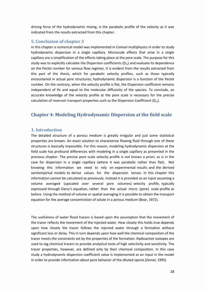
List of tables Table 1: Hydrodynamic dispersion coefficient for different times and Peclet numbers with
parabolic and flat velocity profiles in a capillary ..................................................................... 27
Table 2: Permeability in x, y, z direction in the three layers of the reservoir ......................... 35
Table 3: Permeability in x, y, z directions of the two phase flow reservoir ............................ 53
Table 4: Parameters implemented for the three dimensional; two phase flow reservoir
model ....................................................................................................................................... 53
Table 5: Gravity effect added in the third component of velocity; with the use of the two
Darcy’s interface of Comsol Multiphysics. .............................................................................. 53
Acknowledgements I place on record, my sincere thank you to Dr. Ch.Chatzichristos and Dr. A. Yiotis, for their
support and encouragement.
I would like to thank the School of mineral resources of the faculty of engineering of Crete
for the opportunity to conduct my Msc thesis on the National Center of Scientific Research
“DEMOKRITOS”.
I would also like to thank my family and Eirini for their support and patience.
Abstract The numerical modeling of transport processes in stratified petroleum reservoirs is a task of
significant importance in the oil production industry as it is involved in technologies
related to both reservoir characterization and recovery optimization. Traditional modeling

7
approaches rely on the treatment of the porous material of the reservoir as an effective
continuum, where fluxes are related to the gradients of volumed-average scalar
properties, such as pressure, concentration, phase saturation and temperature, through
macroscopic (cores scale) parameters, such as the medium permeability (or relative
permeabilities for multi-phase flows), effective diffusivities etc. Such approaches essentially
ignore the accurate description of pore scale phenomena arising at the complicated
geometry of the pore scale in favor of reduced computational time for such field scale
problems.
Modeling of transport processes at the pore scale is however an indispensable tool for the
calculation of macroscopic transport parameters, as an alternative to core and field scale
experimental measurements. The objective of this Msc thesis, is thus to offer better
physical insight on how pore scale effects such as hydrodynamic dispersion determine
the field scale transport properties in such upscaled systems. This will be accomplished
using a commercially available generic finite element solver numerical modeling tool;
Comsol Multiphysics. The results will be then implemented at realistic reservoir scale
systems to study two processes relevant to reservoir characterization and recovery
optimization; non-Gaussian hydrodynamic dispersion and water-flooding.
Pore-scale modeling is a first step to study single and multiphase flows and transport in
porous media. The hydrodynamic dispersion coefficient is calculated for a single capillary, in
order to simulate the phenomenon emanating at the pore scale. Mass transfer in the field
scale and therefore in three dimensions is simulated in the second model, in order to extract
information about dispersion in three dimensions and about the effects arising in a
stratified, anisotropic and heterogeneous geometry, such as those typically encountered in
petroleum reservoirs. As a last step, two phase flow is simulated in a three dimensional
reservoir focusing primarily on the displacement of the non-wetting (oil) from the wetting
phase (water) in the course of a Waterflooding process, used to optimize oil recovery in
pressure depleted reservoirs.
The above numerical simulations are performed using a commercially-available software;
Comsol Multiphysics. The Comsol multiphysics software utilizes PDEs to model the above
physical phenomena. The system of equations, which are implemented in the software,
consists of mass balances, partial differential equations that describe the accumulation,
transport, injection and production of the phases in the model. In addition, several auxiliary
equations apply to the system, coupling the different phases in the system together. This set
of equations, PDEs and auxiliary equations, allows for equation manipulation such that the
main differences between the formulations are the dependent variables that are solved for.
A comparison with the results of Eclipse simulator, which is widely used in the oil recovery
industry, will be also provided in the case of two phase flow in a petroleum reservoir. Finally
the aim is to evaluate the possibility of whether Comsol Multiphysics can reproduce the
results provided by commercial reservoir simulators such as Eclipse 100.

8
Chapter 1: An introduction to transport processes in Petroleum
Reservoirs
1. Petroleum Reservoir A petroleum reservoir or oil and gas reservoir is a subsurface quantity of hydrocarbons
contained in porous or fractured rock formations. The naturally occurring hydrocarbons,
such as crude oil or natural gas, are trapped in the subsurface by overlying rock formations
with lower permeability (caprocks). The total estimate of petroleum reservoirs includes the
total quantity of oil that be can be recovered and oil residuals that cannot be recovered, due
to geographical constraints and reservoir/oil characteristics and financial/technological
limitations. The fraction of crude oil reservoirs that can be extracted from the oil field using
current technology is classified as reserves. In order to maximize the oil recovery from a
field, various techniques are used during the lifetime of a reservoir.
2. Oil Recovery technologies Oil recovery technologies can be divided into three different types, which are explained
below. Water injection is a secondary recovery method.
Primary recovery is the natural depletion of the reservoir (Green and Willhite, 1998).This
means that oil is recovered with the help of the natural energy present in the reservoir,
namely the pressure build-up during its formation process. Examples are solution-gas drive,
gas-cap drive, natural water drive, fluid and rock expansion and gravity drainage. This form
of production is used at the beginning of a reservoirs production period. Primary recovery is
the least expensive method of extraction and typical recovery factors during this process is
5-15% of original oil in place (OOIP).
Secondary recovery is the augmentation of natural energy with the injection of water or gas
(Green and Willhite, 1998).The mechanism relies on the maintenance of pressure or a
mechanical displacement of fluids. The most common secondary recovery method today is
water injection, typically termed water-flooding, but gas injection is also used.
Tertiary recovery is often called “Enhanced Oil Recovery” or EOR for short.(Green and
Willhite, 1998). This form of recovery affects the residual oil saturation to increase oil
recovery. Tertiary processes can be CO2, surfactant, polymer or low salinity injection. The
common denominator is that they change the interaction between the injected fluid and the
reservoir fluid.
3. Reservoir Characterization by tracers injection Tracers are chemical substances that are applied in minor quantities in an oil recovery
process in order to keep track of fluid flow, characterize the reservoir formation and
eventually assist in the selection of optimal recovery strategies .They are ideally inert

9
compounds, which follow only the fluid under investigation. They are used widely by the oil
industry for reservoir monitoring and improved reservoir description.
The aforementioned oil recovery and reservoir characterization technologies rely on the
complicated interplay of a series of transport processes with the typically heterogeneous
and anisotropy pore structure of petroleum reservoirs. These transport processes include
both immiscible and miscible two-phase (oil-water) and three-phase (oil-water-gas) flows,
hydrodynamic dispersion of tracers and dissolved species and energy transfer (mechanical
and heat) over extended length scales. The rigorous numerical modeling of such processes
at the pore and field scales is thus of crucial importance on the characterization of oil
reservoirs and the development of novel oil recovery technologies. The modeling of such
transport processes, typically encountered during secondary oil recovery, is the main
objective of this thesis, as will be discussed in more detail below.
4. Objectives of this MSc thesis Waterflooding and water-based floods are the most widely used secondary recovery
methods. In cases where the water entering the field comes from many different sources,
managing the waterfloods operation can become difficult. The addition of a tracer to the
injected water is the only means of distinguishing between injection water and formation
water, or between waters from different injection wells in the same field. Tracers are added
to waterfloods for many reasons and in a variety of circumstances. (Zemel, 1995) They can
be a powerful tool for describing the reservoir, investigating unexpected anomalies in flow,
or verifying suspected geological barriers or flow channels. They can also be used in a test
section of the field before expanding the flood. Flow in most reservoirs is anisotropic. The
reservoir structures are usually layered and frequently contain significant heterogeneities
leading to directional variations in the extent of flow. As a result, the manner in which water
moves in the reservoir can be difficult to predict. Tracers are used in enhanced oil recovery
pilot tests to monitor the actual water-flow pattern during the test. The ability to identify
the water source is basic to the use of tracers for all the purposes described above. The
tracer response as a function of position and time provides a qualitative description of fluid
movement that can play a useful part in managing the flood and thus the recovery
mechanism of the oil in a specific reservoir. These particular transport processes will be the
main focus of this thesis. The objective is to offer better physical insight on how pore scale
effects such as hydrodynamic dispersion determine the field scale transport properties in
such upscaled systems. This will be accomplished using a commercially available generic
finite element solver numerical modeling tools; Comsol Multiphysics. A comparison with the
results with the numerical simulator Eclipse, which is widely used in the oil recovery
industry, will be also attempted.
Chapter 2: Numerical modeling using Comsol Multiphysics. Comsol Multiphysics is a powerful interactive environment used to model and solve all kinds
of scientific and engineering problems. With this software conventional models for one type
of physics can easily be extended into multiphysics models that solve coupled physics
phenomena and do so simultaneously.

10
Using predefined Comsol’s interfaces, it is possible to build models by defining the relevant
physical quantities such as material properties, loads, constraints, sources, and fluxes rather
than defining the underlying equations. The software internally compiles a set of equations
representing the entire model through a flexible graphical user interface or by script
programming in Java or the Matlab language.
Using these physics interfaces, you can perform various types of studies including:
• Stationary and time-dependent (transient) studies
• Linear and nonlinear studies
• Eigenfrequency, modal, and frequency response studies
When solving the models, Comsol assembles and solves the problem using a set of advanced
numerical analysis tools. The software runs the analysis together with adaptive meshing and
error control using a variety of numerical solvers. Furthermore creates sequences to record
all steps that create the geometry, mesh, studies and solver settings, and visualization and
results presentation. It is therefore easy to parameterize any part of the model with the use
of the software’s interface. The Software use Partial differential equations (PDEs) form the
basis for the laws of science and provide the foundation for modeling a wide range of
scientific and engineering phenomena.(COMSOL, 2013)
Finite Element Method theory The Finite Element Method is a mathematical approach in which a continuum problem can
be solved by dividing the solution domain into smaller spatial elements. These elements,
termed as finite elements, have the same properties with the original equations, but they
are simpler to define and to reduce the number of unknowns (Huebner, 2001).
The division results in elements composed by edges and nodes which are points of
interception and connection between elements. The solution of differential equations
regarding the physical problem can be solved by approximated functions that satisfy the
conditions described by integral equations in the problem domain. These approximated
functions are usually polynomial functions (Huebner, 2001).
In FEM there are two ways to solve problems described as partial differential equations. The
so-called "strong form" is the direct resolution of the equations. The "weak form" has
evolved from approximated numerical methods that are integral representations of
differential equations governing the physical problem. The “strong form” requires continuity
in the solution of dependent variables so it’s more difficult to work with. The “weak form”
allows a unique method to solve different types of problems because the methods to
transform differential equations in an integral form are generics that usually provide more
precise results. Due to its advantages in complex geometries it is the most used form (Liu,
2003).
The general steps of the Finite Element Method are described as follows:

11
The first step consists in the division of the body in small elements. The type, size and
number of elements are in the field of the engineer judgment but can be supported with
research. Next step is to choose interpolation functions. It is defined in the element using
the nodal values of the element. The most common functions are linear, quadratic and cubic
polynomials, because they are simple to work with. The degree of the polynomial varies
according to the number and nature of nodes of the elements and the unknowns at each
node. The following step is to set the matrix equations. For this, various methods can be
used. In order to obtain the final and global equation for the system, the next step is to
collect and assemble the equations for the element properties. Previously to solving the
system of equations, the equations have to be changed so that it can regard the boundary
conditions. The assemblage results in a group of equation with unknown nodal values,
degrees of freedom. The kind of equations to be solved depends on the type of problem and
if it is time dependent or not. In the end, other parameters dependent of those calculated
can be also obtained. Those parameters are also referred as derived values and can be
volume, surface averages or integrations or simply just point evaluation of certain
quantities. (Huebner, 2001).
Chapter 3: Hydrodynamic dispersion in a single capillary
1. Introduction The phenomenon of hydrodynamic dispersion occurs in problems of underground mixing of
water of different quality in petroleum reservoirs during injection processes. In these
problems, any identifiable solute may serve as a tracer whose concentration distribution
indicates the mixing.
The nature of dispersion or miscible displacement in porous media may be examined from
both an over-all, or macroscopic, and a local, or microscopic, view-point. Because of the
complexities of the structure of such media, there are difficulties associated with both
approaches. Overall behavior, such as the average concentration distribution at the system
outlet as a function of time, can be observed in sets of experiments, as is frequently done in
practice, and the results can be correlated with the variables investigated on empirical or
semi empirical bases. The objective of this case study is to distinguish the progress made in
one attempt to identify the mechanisms of dispersion and miscible displacement in a single
capillary. Because the geometry of the microstructure is generally too complex to be
described by a single model, a simplification is been made by examining the evolution of
those phenomena in a pipe in order to simulate the effects occurring in a single pore. The
medium is considered to consist of a microstructure made up of the pores and void spaces in
and between the solid materials. This requires that the important mechanisms controlling
the transport are identified through experiment so that realistic microstructure models may
be developed.
To implement macroscopically correct laws for describing miscible displacements,
knowledge of local behavior is required, since integral results which reflect overall behavior
are obtained from integrating the differential equations which are assumed to describe local
behavior. It is assumed that the microscopic equations of change are accurate enough to
12
describe phenomena as they occur in a porous medium. However, the application of these
equations to porous media is difficult. Consider the flow boundaries in even the most
orderly packed bed, and the geometric complexities are clear.
Finally, the microscopic results need to be combined and averaged so that a comparison
with macroscopic behavior can be attained. At this point, the theory is intimately related to
experiment since, it is necessary to compare experimental measurements with analytic
solution in order to evaluate the quality of the results.
The model of dispersion in porous media, introduces a new mechanism of spreading of the
tracer that is due to the different rates of advance of the tracer in capillaries of different
orientations. This mechanism can bring about much greater spreading than Taylor’s
dispersion in individual capillary tubes.
The dispersion coefficient, which is a measure of the rate at which material will spread out
axially in the system, is enhanced by having large differences in velocity exist across the flow
and by taking place in equipment with large transverse dimensions. In contrast, any
mechanism which increases transverse mixing, such as turbulence or transverse convection
currents, reduces the dispersion coefficient. These arguments apply, in a qualitative way, to
porous media as well as to simple configurations. That is, in porous media, dispersion is
created by both the microscopic differences in velocity which exist in the interstices
between particles and by large-scale or macroscopic effects such as channeling (Dullien,
1979; Nunge, and Gill, 1969).
2. Transport equations for Hydrodynamic Dispersion Dispersion phenomena occur in many important fields of technology, for example, in
petroleum reservoir engineering, ground water hydrology, chemical engineering,
chromatography. A few examples are so called miscible flood in petroleum recovery;
transition zone between salt waste disposal into acquifers; radio activate and ordinary
sewage soil; packed reactors in chemical industry; use of various ‘tracers’ in petroleum
engineering and hydrology research projects, etc.
The treatment of hydrodynamic dispersion is divided here in two main sections: Dispersion
in a capillary tube and dispersion in a porous medium. The reasons for examining the
dispersion process in a capillary are twofold. First, the phenomenological equations
describing dispersion are often the same as in the case of a porous medium. Second,
dispersion in a capillary tube, the mechanism of which is relatively well understood, plays a
role in determining dispersion in porous media.
In this chapter the following process takes place; A solvent (water) is flowing in long capillary
under steady state conditions at low Reynolds numbers. A second species (tracer) is
completely dissolved in the flow stream to form a solution. Τhe tracer concentration is
spatially variable, but always at the dilute limit. Namely, the tracer concentration does not
affect the bulk phase (solvent) properties. Therefore properties of solvent are the same as
the properties of solution before the injection of the tracer.

13
The hydrodynamic dispersion process is then determined by the equations for the flow of
the solution and the mass conservation of the diluted species.
Navier Stokes equation: Momentum Conservation
The Navier-Stokes equations govern the motion of fluids and can be seen as Newton's
second law of motion for fluids. In the case of a compressible Newtonian fluid, this yields
ρ(𝜕𝑢
𝜕𝑡 + u*u) = -p + *(μ(u + (u)T) -
2
3μ(*u)) + F (3.1.1)
Where u is the fluid velocity, p is the fluid pressure, ρ is the fluid density, and μ is the fluid
dynamic viscosity. The different terms correspond to the inertial forces (first term), pressure
forces (second), viscous forces (third), and the external forces applied to the fluid (forth).
The Navier-Stokes equations were derived by Navier, Poisson, Saint-Venant, and Stokes
between 1827 and 1845.
In the limit of low Reynolds numbers Re->0 and under steady state conditions, which is
typically the case for pore media flows, the acceleration terms (on the left-hand of
Eq.(3.1.1)) are negligible, and thus the above equation reduces to the Stokes equation;
p=*(μ(u + (u)T) - 2
3μ(*u)) + F (3.1.2)
These equations are always solved together with the continuity equation:
𝜕𝜌
𝜕𝑡 + *(ρu) = 0 (3.2.1)
Equation (3.2.1) for the typical case of an incompressible fluid under steady state conditions
reduces to:
*u=0 (3.2.2)
The Navier-Stokes (or Stokes) equations represent the conservation of momentum, while
the continuity equation represents the conservation of mass for the solution (water and
dissolved tracer).
Mass Balance Equation - Mass conservation of diluted species
The Transport of diluted species at the pore space is governed by diffusion and convection
as described by the following equation:
∂c
∂t + uc = *(Dc) + R (3.3)
c is the concentration of the species (mol/m3 )
D denotes the diffusion coefficient (m2/s)
R is a reaction rate expression for the species (mol/(m3 ·s))
u is the velocity vector ( m/s)
14
The first term on the left-hand side of Equation (3.3) corresponds to the accumulation of the
species.
The second term accounts for the convective transport due to a velocity field u. This field
can be expressed analytically or be obtained from coupling this physics interface to one that
describes fluid flow (momentum balance). To include convection in the mass balance
equation, an expression that includes the space and time variables, or the velocity vector
component variable names from a fluid flow physics interface of Comsol, can be entered
into the appropriate field. The velocity fields from existing fluid flow interfaces are available
directly as predefined fields (model inputs) for multiphysics couplings.
On the right-hand side of the mass balance equation (3.3.1), the first term describes the
diffusive transport, accounting for the interaction between the dilute species and the
solvent. A field for the diffusion coefficient is available, and any expression containing other
variables such as pressure and temperature can be entered here. The node has a matrix that
can be used to describe anisotropic diffusion coefficients.
Finally, the second term on the right-hand side of Equation (3.3.1); represents a source or
sink term, typically due to a chemical reaction. In order for the chemical reaction to be
specified, another node must be added to Comsol’s Transport of Diluted Species interface
the Reaction node, which has a field for specifying a reaction equation using the variable
names of all participating species. (COMSOL Multiphysics 2015)
Dispersion in a single Capillary
The simplest model for characterizing the microstructure in porous materials is the straight
tube. Bundles of straight capillaries have long been used to model flow through porous
media and assemblages of randomly oriented straight pores or capillaries, where it is
assumed that the path of a marked element consists of a sequence of statistically
independent steps, direction and duration of which vary in a random manner. Here the
results of capillary dispersion are considered for the purpose of illustrating the interactions
of some of the factors influencing dispersion in porous media. The straight tube provides a
well-defined hydrodynamical system where the dispersion process is most easily described
while still retaining many of the main features of the same process in porous media.
Consider first the dispersion of two fluids of the same constant physical properties in a
straight capillary tube with steady fully developed laminar flow prevailing. An early
experimental work which demonstrated the essence of the process without mathematical
treatment was reported by Griffiths in 1911, who observed that a tracer injected into a
stream of water spreads out in a symmetrical manner about a plane in the cross section
which moves with the mean speed of flow. This is a rather startling result for two reasons.
First, since the water near the center of the tube moves with twice the mean speed of flow
and the tracer at the mean speed, the water near the center must approach the column of
tracer, absorb the tracer as it passes through the column, and then reject the tracer as it
leaves on the other side of the column. Second, although the velocity is unsymmetrical
about the plane moving at the mean speed, the column of tracer spreads out symmetrically.
The concentration of the tracer material is described by the two-dimensional unsteady
convective diffusion equation, equation (3.4).
15
𝜕𝑐
𝜕𝑡 + u(r)
𝜕𝑐
𝜕𝑥 = Ɗ(
𝜕2𝑐
𝜕𝑥2 +
1
𝑟
𝜕
𝜕𝑟𝑟
𝜕𝑐
𝜕𝑟) (3.4)
Here C is the point concentration, u the parabolic laminar velocity profile, and x and r the
axial and radial coordinates, respectively. Taylor showed that for a large enough number of
times the process could be described by a one-dimensional dispersion model, as given in
equation (3.5).
𝜕ĉ
𝜕𝑡 + ū
𝜕ĉ
𝜕𝑥 = Dct
𝜕2ĉ
𝜕𝑥2 (3.5)
Upon defining a coordinate which moves with the mean speed of flow as:
x’ =x – ūt (3.6)
Equation (3.5) becomes
𝜕ĉ
𝜕𝑡 = Dct
𝜕2 ĉ
𝜕𝑥′2 (3.7)
The above equation is simply the one-dimensional unsteady diffusion equation to which
solutions are readily available under a variety of conditions. The molecular diffusion
coefficient has been replaced by an effective axial diffusion coefficient or dispersion
coefficient which, in the absence of axial molecular diffusion, Taylor showed to be
K= 4𝑎2𝑢𝑚
2
192𝐷 (3.8.1)
K=Dct (3.8.2)
Where α is the tube radius. This simple equation provides a great deal of physical insight
into the nature of the dispersion process if we interpret the numerator to be a measure of
axial convection and the denominator to reflect the intensity of transverse mixing rather
than just transverse molecular diffusion.
The solution of the (3.5) equation, known as second law of diffusion, is well known for the
case under consideration:
Ĉ
𝐶𝑜 =
1
2(𝜋∗𝐷𝑐𝑡∗𝑡)exp[−
(𝑥−ū∗𝑡)2
4𝐷𝑐𝑡∗𝑡] (3.6)
Where c0 is the initial tracer concentration in the slug and Dct=σχ2/2t, with σx the standard
deviation of the Gaussian distribution of the tracer concentration. Therefore, the length of
the mixed zone in Figure 1 keeps increasing symmetrically on both sides of the tracer
concentration maximum in the middle of the slug. The concentration tapers off to zero at
both ends of the slug.

16
Figure 1: Schematic representation of the mixed zone for A dispersing in B as function of time [Dullien, 1979]
In this event, we see that the dispersion coefficient, which is a measure of the rate at which
material will spread out axially in the system, is enhanced by having large differences in
velocity exist across the flow and by taking place in equipment with large transverse
dimensions. In contrast, any mechanism which increases transverse mixing, such as
turbulence or transverse convection currents, reduces the dispersion coefficient. These
arguments apply, in a qualitative way, to porous media as well as to simple configurations.
That is, in porous media, dispersion is created by both the microscopic differences in velocity
which exist in the interstices between particles and by large-scale or macroscopic effects
such as channeling. Aris later extended the analysis to include axial molecular diffusion and
demonstrated that the dispersion coefficient for this case contains Taylor’s result with an
additive term due to diffusion. (Dullien, 1979)
k = D + 4𝑎2∗𝑈𝑚2
192𝐷 (3.7)
This combined result will be referred to as the Taylor-Aris theory. It is important to note the
restriction placed on the Taylor-Aris theory with respect to time, since, unless this time is
exceeded, the mean concentration distribution is not described by a dispersion model. For
porous media, the dimension in the flow direction must be large enough to ensure sufficient
residence time for a dispersion model to apply.
The formal analogy of Equation (3.6) with Fick’s second law of diffusion may easily lead to
the false conclusion that in hydrodynamic dispersion the driving force of spreading of the
tracer is the axial concentration gradient ∂caverage /∂x’, which in the reality is a result of an
interplay between axial convection and radial diffusion. In other words is the effect rather
than the cause of the process.
For the case of negligible axial molecular diffusion, Taylor showed Dct to be given as
Dct=R2 ū 2/48 Ɗ = Pect 2 Ɗ/192 (3.8)
Where Dct includes the effect of both mechanical and (or convective) dispersion and radial
molecular diffusion. It is enlightening to note that as Ɗ→ oo, Dct → 0 and as Ɗ →0, Dct → oo.

17
Hence, very intense radial mixing eliminates dispersion and the absence of radial mixing
results in a infinite dispersion coefficient.
Aris (1956), however, showed that when the axial molecular diffusion is not negligible, the
axial dispersion coefficient contains an additive term due to diffusion.
Dct= Ɗ + R2 ū2/48 Ɗ= Ɗ + (Pect2/192) (3.9)
Inspection of Equations (3.8) and (3.9) shows that the rate of spreading (dispersion)
increases rapidly with tube diameter and velocity, and it decreases with increasing diffusion
coefficient, at least as long as R2 ū 2/48 Ɗ is much greater than Ɗ. (Dullien, 1979)
3. Model Implementation in Comsol Multiphysics In the following case study, the Navier-Stokes equations and the mass conservation equation
are numerically solved in a computational domain, such as the one shown in Figure 2. In
order for those equations to be implemented in Comsol multiphysics two interfaces where
utilized, namely Laminar flow interface and Transport of diluted species interface.
Furthermore, the differential equations need to be solved with a set of boundary conditions.
At the next figure the 2D Axisymmetric Pipe Flow geometry is illustrated.
Figure 2: Axisymmetric Pipe flow, Capillary Dimensions (Height 0.2, Width 0.01 m)
Laminar flow interface
Pressure is specified as 1e5+0.0005 Pa at the inlet and as 1e5 Pa at the outlet. A no-slip
boundary condition (i.e., the velocity is set to zero) is specified at the side walls of the
capillary. The numerical solution of the steady-state NS (the time-dependent derivative is set
to zero) and continuity equations in the laminar regime and for constant boundary
conditions.
18
Transport of diluted species interface
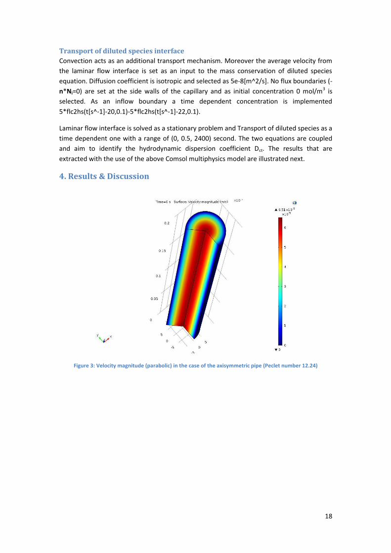
Convection acts as an additional transport mechanism. Moreover the average velocity from
the laminar flow interface is set as an input to the mass conservation of diluted species
equation. Diffusion coefficient is isotropic and selected as 5e-8[m^2/s]. No flux boundaries (-
n*Ni=0) are set at the side walls of the capillary and as initial concentration 0 mol/m3 is
selected. As an inflow boundary a time dependent concentration is implemented
5*flc2hs(t[s^-1]-20,0.1)-5*flc2hs(t[s^-1]-22,0.1).
Laminar flow interface is solved as a stationary problem and Transport of diluted species as a
time dependent one with a range of (0, 0.5, 2400) second. The two equations are coupled
and aim to identify the hydrodynamic dispersion coefficient Dct. The results that are
extracted with the use of the above Comsol multiphysics model are illustrated next.
4. Results & Discussion
Figure 3: Velocity magnitude (parabolic) in the case of the axisymmetric pipe (Peclet number 12.24)
19
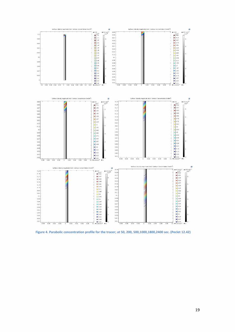
Figure 4. Parabolic concentration profile for the tracer; at 50, 200, 500,1000,1800,2400 sec. (Peclet 12.42)

20
Figure 5: Flat concentration profile for the tracer; at 50, 200, 500, 1000, 1800, 2400 sec. (Peclet 12.42)
21
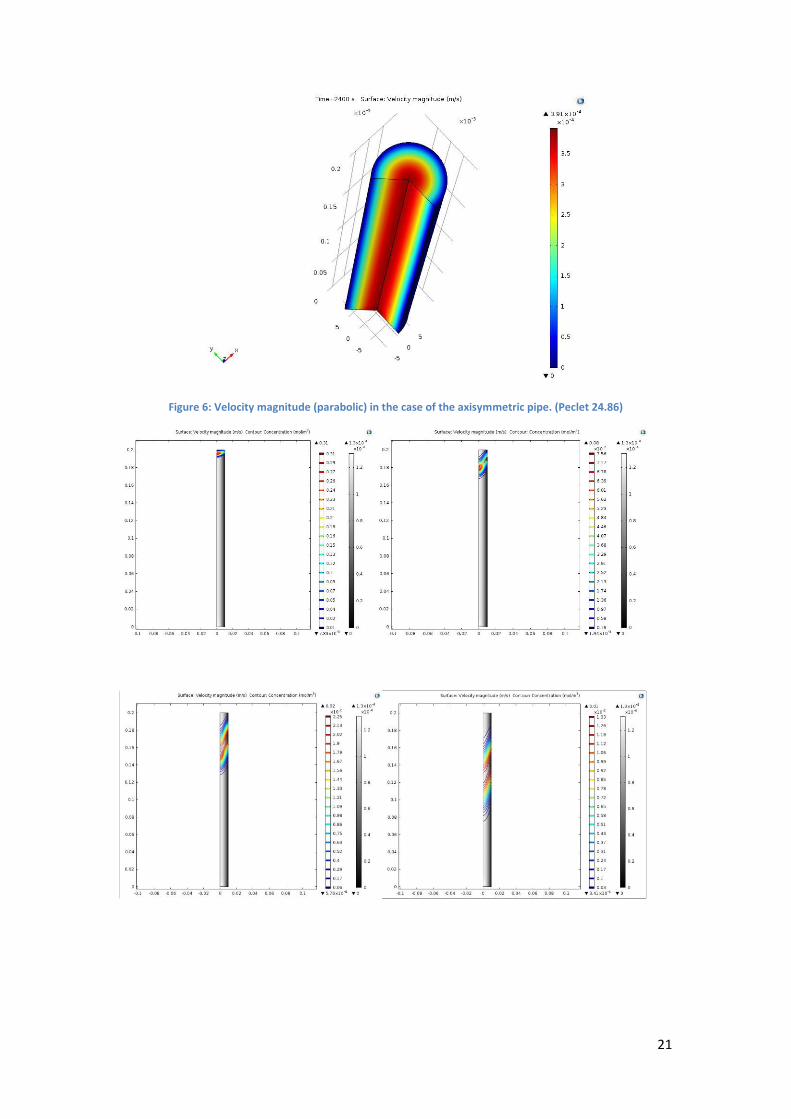
Figure 6: Velocity magnitude (parabolic) in the case of the axisymmetric pipe. (Peclet 24.86)
22
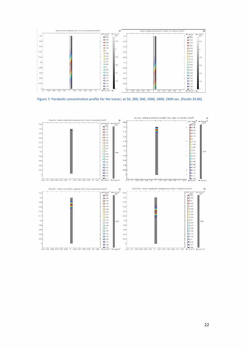
Figure 7: Parabolic concentration profile for the tracer; at 50, 200, 500, 1000, 1800, 2400 sec. (Peclet 24.86)

23
Velocity profile (Parabola-Flat)
The solution of the NS equation in a such a capillary yields a parabolic velocity profile
with an analytical solution described by Eq.(3.10). This particular velocity profile significantly
enhances the mixing of diluted species in the direction parallel to the flow due to the
development of concentration gradients in the transverse direction. These combined
effected lead to longitudinal (in the flow direction) dispersion coefficients that are
always higher that the molecular diffusion coefficient and a function of the Peclet number
as discussed above.
Neglecting the exact velocity profile at the pore scale, as is typically the case in field (Darcy)
scale modeling essentially leads to the assumption of a flat (piston-like) velocity profile at
the pore scale where the dispersion coefficient is always equal to molecular diffusivity. In
the case, therefore, of Darcy scale modeling the exact values for the dispersion coefficient
tensor should be given as input, being previously evaluated either experimentally or using
rigorous pore scale modeling.
The effects of pore scale velocity profiles are thus discussed below. Equations
describing Paraboloid and Flat velocity of the flow acting inside the capillary:
Paraboloid velocity Flat velocity
u(r)= (𝑅2− 𝑟2
4𝜇)𝛥𝑃
𝐿 (3.10) u(r)=
𝑅2
8𝜇 𝛥𝑃
𝐿 (3.11)
Figure 8: Flat concentration profile for the tracer; at 50, 200, 500, 1000, 1800, 2400 sec.(Peclet 24.86)
24
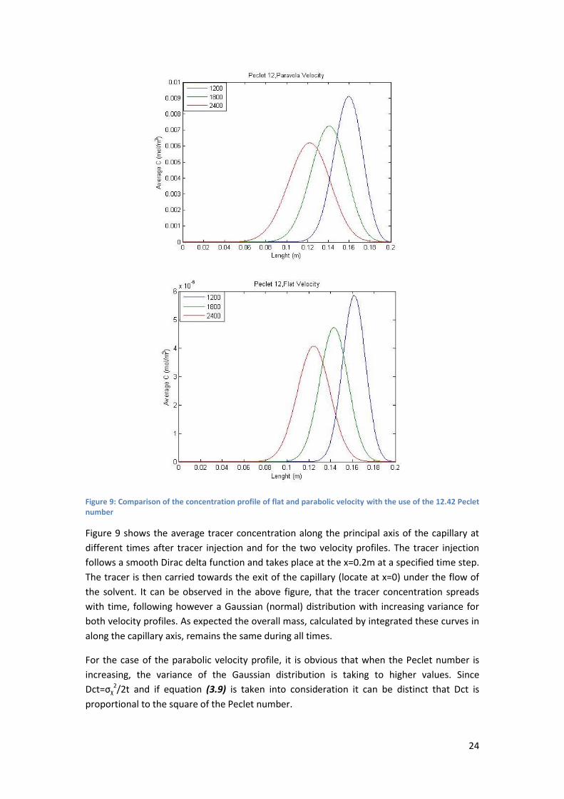
Figure 9: Comparison of the concentration profile of flat and parabolic velocity with the use of the 12.42 Peclet number
Figure 9 shows the average tracer concentration along the principal axis of the capillary at
different times after tracer injection and for the two velocity profiles. The tracer injection
follows a smooth Dirac delta function and takes place at the x=0.2m at a specified time step.
The tracer is then carried towards the exit of the capillary (locate at x=0) under the flow of
the solvent. It can be observed in the above figure, that the tracer concentration spreads
with time, following however a Gaussian (normal) distribution with increasing variance for
both velocity profiles. As expected the overall mass, calculated by integrated these curves in
along the capillary axis, remains the same during all times.
For the case of the parabolic velocity profile, it is obvious that when the Peclet number is
increasing, the variance of the Gaussian distribution is taking to higher values. Since
Dct=σχ2/2t and if equation (3.9) is taken into consideration it can be distinct that Dct is
proportional to the square of the Peclet number.

25
A graphical summary of the regions of applicability of various analytical solutions for
dispersion for the step change in inlet concentration has been given by Nunge and Gill
(1969) (Figure 11) with the τ=tƊ/R2 and the Peclet number Pect=2Rū/Ɗ as parameters. An
important point is relating to the dispersion model is that τ must be sufficient large for it to
apply. For example 0.8 for fully developed laminar flow in tubes.
The comparison between the concentration distributions for the two velocity profiles reveals
that, while the average position of the distribution is the same in both cases, the variance
increases more rapidly in the case of the parabolic velocity profile, demonstrating the
important effects of microscale velocity on hydrodynamic dispersion.
Figure 10: Comparison of the concentration profile of the parabolic and flat velocity with the use of 24.86 Peclet number

26
Figure 11: Summary of the regions of applicability of various analytical solutions for dispersion in capillary tubes with a step change in inlet concentration as a function of τα and Pect. [Dullien, 1979]
At high Peclet numbers with the same fluids, a straight channel having the same equivalent
diameter (four times the hydraulic radius) as a tube requires a minimum real time of
approximately 1/3 of that for the tube before the dispersion model applies, thus indicating
that the minimum real time requirement is a strong function of the geometry of the system.
The Concentration profiles of figures 9 & 10 were used as an input in the curve fitting tool of
Matlab. Standard deviation of each Gaussian profile was computed as a next step. Since the
coefficient of hydrodynamic dispersion follows the Dct=σ2/2*t formulation, where t is the
time that slug disperse in the stream of water, three specific times were selected in each
case for the calculation of Dct. Dimensionless time (τ =t*D/R2) also is computed for 1200,
1800, 2400 sec and the results are presented in the next table. The analytic solution which is
used for verification is Dct = 9.02*10-8 m2/s.
27
Parabolic Velocity Profile Flat Velocity Profile
Peclet 12.43 Dimensionless Peclet 12.43 Dimensionless
Time Dct(10-8 m2/s) Τime (τ) Time Dct(10-8 m2/s) Τime (τ)
1200 7,79 0,6 1200 4,64 0,6
1800 8,17 0,9 1800 4,75 0,9
2400 8,37 1,2 2400 4,81 1,2
Parabolic Velocity Profile Flat Velocity Profile
Peclet 24.86 Dimensionless Peclet 24.86 Dimensionless
Time Dct(10-7 m2/s) Time (τ) Time Dct(10-8 m2/s) Τime (τ)
1200 1,97 0,6 1200 4,85 0,6
1800 2,02 0,9 1800 4,9 0,9
2400 2 1,2 2400 4,92 1,2 Table 1: Hydrodynamic dispersion coefficient for different times and Peclet numbers with parabolic and flat velocity profiles in a capillary
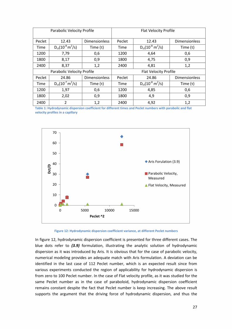
Figure 12: Hydrodynamic dispersion coefficient variance, at different Peclet numbers
In figure 12, hydrodynamic dispersion coefficient is presented for three different cases. The
blue dots refer to (3.9) formulation, illustrating the analytic solution of hydrodynamic
dispersion as it was introduced by Aris. It is obvious that for the case of parabolic velocity,
numerical modeling provides an adequate match with Aris formulation. A deviation can be
identified in the last case of 112 Peclet number, which is an expected result since from
various experiments conducted the region of applicability for hydrodynamic dispersion is
from zero to 100 Peclet number. In the case of Flat velocity profile, as it was studied for the
same Peclet number as in the case of paraboloid, hydrodynamic dispersion coefficient
remains constant despite the fact that Peclet number is keep increasing. The above result
supports the argument that the driving force of hydrodynamic dispersion, and thus the
0
10
20
30
40
50
60
70
0 5000 10000 15000
Dct
/D
Peclet ^2
Aris Forulation (3.9)
Parabolic Velocity,Measured
Flat Velocity, Measured
28
driving force of the hydrodynamic mixing, is the parabolic profile of the velocity as it was
indicated from the results extracted from this chapter.
5. Conclusion of chapter 3 In this chapter a numerical model was implemented in Comsol multiphysics in order to study
hydrodynamic dispersion in a single capillary. Microscale effects that arise in a single
capillary are a simplification of the effects taking place at the pore scale. The purpose for this
study was to explicitly calculate the Dispersion coefficients (Dct) and evaluate its dependence
on the Peclet number for various flow regimes. It is evident from the results extracted from
this part of the thesis, which for parabolic velocity profiles, such as those typically
encountered in actual pore structures; hydrodynamic dispersion is a function of the Peclet
number. On the contrary, when the velocity profile is flat, the Dispersion coefficient remains
independent of Pe and equal to the molecular diffusivity of the species. To conclude, an
accurate knowledge of the velocity profile at the pore scale is necessary for the precise
calculation of reservoir transport properties such as the Dispersion Coefficient (Dct).
Chapter 4: Modeling Hydrodynamic Dispersion at the field scale
1. Introduction The detailed structure of a porous medium is greatly irregular and just some statistical
properties are known. An exact solution to characterize flowing fluid through one of these
structures is basically impossible. For this reason, modeling hydrodynamic dispersion at the
field scale has profound differences with modeling in a single capillary as presented in the
previous chapter. The precise pore scale velocity profile is not known a priori, as is in the
case for dispersion in a single capillary (where it was parabolic rather than flat). Not
knowing this information we need to rely on experimental results and the derived
semiempirical models to derive values for the dispersion tensor. In this chapter this
information cannot be calculated as previously. Instead it is provided as an input assuming a
volume averaged (upscaled over several pore volumes) velocity profile, typically
expressed through Darcy’s equation, rather than the actual micro (pore) scale profile as
before. Using the method of volume or spatial averaging it is possible to obtain the transport
equation for the average concentration of solute in a porous medium (Bear, 1972).
The usefulness of water flood tracers is based upon the assumption that the movement of
the tracer reflects the movement of the injected water. How closely this holds true depends
upon how closely the tracer follows the injected water through a formation without
significant loss or delay. This in turn depends upon how well the chemical composition of the
tracer meets the constraints set by the properties of the formation. Radioactive isotopes are
used to tag chemical tracers to provide analytical tools of high selectivity and sensitivity. The
tracer properties, however, are defined only by their chemical composition. In this case
study a hydrodynamic dispersion coefficient value is implemented as an input in the model
in order to provide information about pore behavior of the diluted specie.(Zemel, 1995)

29
Firstly the direction of flow from the injector towards the producer can be identified.
Furthermore the parts of the reservoir where the total velocity is greater can be distinct. The
overall behavior of the reservoir is verified with the use of the dispersion of the tracer in
three dimensions. The macroscopic results are linked with the pore behavior that was
presented at chapter three. The only difference in this chapter is that dispersion takes place
in three dimensions and in order for this behavior to be quantify longitudinal and transverse
dispersion (parallel and vertical to the direction of flow) are predefined. When the model is
set and verified, contour plots are illustrates to provide information about the behavior of
the tracer during the injection of water in the life of the reservoir. Normal total flux that is
removed from the reservoir in various times is plotted as well. Moreover the total quantity
of mol that exists in the reservoir at each time step is presented in order to identify the
influence of stratified geometry in the model. Finally a contrast is illustrated between two
cases of stratified reservoirs; heterogeneous and homogeneous anisotropic three layered
cases for the Normal total flux (mol/s) and for the Ntotal (mol) existing in the reservoir.
A three dimensional model is implemented in this chapter in order to simulate the mass
transfer of a tracer under the single phase flow of water in a stratified petroleum reservoir.
Prediction of macroscopic transport properties of a porous medium from its geometric
characteristics (e.g. porosity, stratified geometry) is investigated in this case study.
Conservation of momentum in the form of Darcy’s law equation is used to simulate single
phase flow in porous media. Conservation of mass of diluted species at the field scale is
simulated with the use of Comsol’s Diluted Species interface.
2. Transport equations for Hydrodynamic dispersion in porous
media In the case of saturated flow through a porous medium, if in a portion of the flow domain a
certain mass of solute is inserted; this solute will referred as a tracer. Various experiments
indicate that as flow takes place the tracer gradually spreads and occupies an ever-
increasing portion of the flow domain, beyond the region it is expected to occupy according
to the average flow alone. This phenomenon is called hydrodynamic dispersion in a porous
medium. It is a non-steady, irreversible process in which the tracer mass mixes with the
liquid solute. If initially the tracer-labelled liquid occupies a separate region, with an abrupt
change separating it from the unlabeled liquid, this interface does not remain an abrupt one,
the location of which may be determined by the average velocity expressed by Darcy’s Law.
(Bear, 1972)
In general, hydrodynamic dispersion consists of two parts: mechanical dispersion and
molecular diffusion. Mechanical dispersion results from the movement of individual fluid
particles which travel at variable velocities through tortuous pore channels of the porous
medium. The complicated system of interconnected passages comprising the microstructure
of the medium cause a continue subdivision of the tracer’s mass into finer offshoots.
Variation in local velocity, both in magnitude and direction along the tortuous flow paths
and between adjacent flow paths are result of the velocity distribution within each pore. The
random fluid movement in irregular flow paths generates a blended region between the two
fluids. The amount of spreading depends on the dispersive capability of the porous medium.
The property of porous medium that is a measure of its capacity to cause mechanical

30
dispersion is called dispersivity. In general, dispersivity is considered to have two
components: one in the direction of mean flow (longitudinal dispersion) and one
perpendicular to the direction of mean flow (transverse dispersion). For practical purposes,
however, transverse dispersion has a minor effect on the amount of mixing between fluids
compared to longitudinal dispersion. (Bear, 1972; Bear & Bachmat, 1967; Maghsood &
Brigham, 1982)
The second component of hydrodynamic dispersion, molecular diffusion occurs on a
macroscopic level as a consequence of net concentration gradients across surfaces
perpendicular to the average flow direction. It is caused by the random movement of the
differing molecules. This molecular diffusion contributes to the growth of the mixed region
as well.
Darcy’s Equation for momentum transfer in porous media
Darcy’s law equation is actually the momentum conservation equation in this chapter. It can
be derived from the Navier Stokes using volume averaging. The presence of spatial
deviations of the pressure and velocity in the volume-averaged equations of motion gives
rise to representation for the spatial deviations are derived that lead to Darcy's law.
In a porous medium, the global transport of momentum by shear stresses within the fluid is
typically negligible; because the pore walls impede momentum transport to the fluid outside
the individual pores (namely friction with the pore walls is dominant over friction between
adjacent fluid layers). A detailed description, down to the resolution of every pore, is not
practical in most applications. A homogenization of the porous and fluid media into a single
medium is a common alternative approach. Darcy’s law together with the continuity
equation and equation of state for the pore fluid (or gas) provide a complete mathematical
model suitable for a wide variety of applications involving porous media flows, for which the
pressure gradient is the major driving force.
Darcy’s equation describes fluid movement through interstices in a porous medium. Because
the fluid loses considerable energy to frictional resistance within pores, flow velocities in
porous media are very low. The Darcy’s Law interface in the Subsurface Flow Module applies
to water moving in an aquifer or stream bank, oil migrating to a well. Also set up multiple
Darcy’s Law interfaces to model multiphase flows involving more than one mobile phase.
Darcy’s law portrays flow in porous media driven by gradients in the hydraulic potential
field, which has units of pressure. For many applications it is convenient to represent the
total hydraulic potential or the pressure and the gravitational components with equivalent
heights of fluid or head. Division of potential by the fluid weight can simplify modeling
because units of length make it straightforward to compare to many physical data. The
physics interface also supports specifying boundary conditions and result evaluation using
hydraulic head and pressure head. In the physics interface, pressure is always the dependent
variable. Darcy’s law applies when the gradient in hydraulic potential drives fluid movement
in the porous medium. Visualize the hydraulic potential field by considering the difference in
both pressure and elevation potential from the start to the end points of the flow line.
According to Darcy’s law, the net flux across a face of porous surface is

31
u = - 𝑘
𝜇 (p + ρgD) (4.1)
In this equation, u is the Darcy velocity or specific discharge vector (m/s); κ is the
permeability of the porous medium (m2); μ is the fluid’s dynamic viscosity (Pa·s); p is the
fluid’s pressure (Pa) and ρ is its density (kg/m3); g is the magnitude of gravitational
acceleration (m/s2); and ∇D is a unit vector in the direction over which the gravity acts. Here
the permeability, κ, represents the resistance to flow over a representative volume
consisting of many solid grains and pores. (COMSOL, 2013).
Transport of Diluted Species in Porous Media
The following equations for the concentrations, ci, describe the transport of solutes in a
variably saturated porous medium for the most general case, when the pore space is
primarily filled with liquid but also contain pockets or immobile gas:
𝜕
𝜕𝑡(θci) +
𝜕
𝜕𝑡(ρbcP,i) +
𝜕
𝜕𝑡(avCG,i) + u*ci = *[(DD,I + De,I)ci]+Ri +Si
(4.2)
On the left-hand side of the above equation, the first three terms correspond to the
accumulation of species within the liquid, solid, and gas phases, while the last term
describes the convection due to the velocity field u (m/s).
ci denotes the concentration of species i in the liquid (mol/m3 ), cP,i the amount adsorbed to
(or desorbed from) solid particles (moles per unit dry weight of the solid), and cG,i the
concentration of species i in the gas phase.
The equation balances the mass transport throughout the porous medium using the porosity
εp, the liquid volume fraction θ; the bulk (or drained) density, ρb = (1 − εp )ρ, and the solid
phase density ρ (kg/m 3 ).
For saturated porous media, the liquid volume fraction θ is equal to the porosity εp , but for
partially saturated porous media, they are related by the saturation s as θ = sεp. The
resulting gas volume fraction is av = εp − θ = (1-s)εp .
On the right-hand side of Equation (4.2), the first term introduces the spreading of species
due to mechanical mixing (dispersion) as well as from diffusion and volatilization to the gas
phase. The tensor is denoted DD (m2 /s) and the effective diffusion by De (m2 /s).
The last two terms on the right-hand side of Equation (4.2) describe production or
consumption of the species; Ri is a reaction rate expression which can account for reactions
in the liquid, solid, or gas phase, and Si is an arbitrary source term, for example due to a fluid
flow source or sink.
n order to solve for the solute concentration of species i, ci , the solute mass sorbed to solids
cP,i and dissolved in the gas-phase cG,i are assumed to be functions of ci.(COMSOL, 2013).
32
Convective Term Formulation
The Transport of Diluted Species in Porous Media interface includes two formulations of the
convective term. The conservative formulation of the species equations in Equation (4.2) as
described before.
If the conservative formulation is expanded using the chain rule, then one of the terms from
the convection part, ci ∇·u, would equal zero for an incompressible fluid and would result in
the non-conservative formulation described in Equation (4.2).
When using the non-conservative formulation, which is the default, the fluid is assumed
incompressible and divergence free: ∇ ⋅ u = 0. The non-conservative formulation improves
the stability of systems coupled to a momentum equation (fluid flow equation). (COMSOL,
2013).
The velocity field to be used in the Model Inputs section on the physics interface can, for
example, be prescribed using the velocity field from a Darcy’s Law Equation interface.
The average linear fluid velocities ua, provides an estimate of the fluid velocity within the
pores:
ua = 𝑢
𝜀𝑝 Saturated (4.3)
ua = 𝑢
𝜃 Partially saturated (4.4)
Where εp is the porosity and θ = s*εp the liquid volume fraction, and S the saturation, a
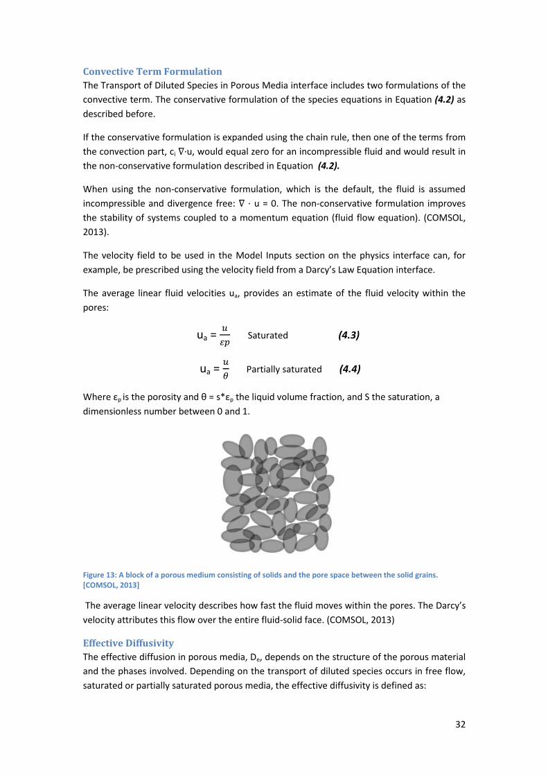
dimensionless number between 0 and 1.
Figure 13: A block of a porous medium consisting of solids and the pore space between the solid grains. [COMSOL, 2013]
The average linear velocity describes how fast the fluid moves within the pores. The Darcy’s
velocity attributes this flow over the entire fluid-solid face. (COMSOL, 2013)
Effective Diffusivity
The effective diffusion in porous media, De, depends on the structure of the porous material
and the phases involved. Depending on the transport of diluted species occurs in free flow,
saturated or partially saturated porous media, the effective diffusivity is defined as:

33
De = 𝜀𝑝
𝜏𝐿DL (4.5)
For a saturated Porous Media
Here DL is the single-phase diffusion coefficients for the species diluted in pure liquid (m2/s),
and τL is the corresponding tortuosity factor (dimensionless).
The tortuosity factor accounts for the reduced diffusivity due to the fact that the solid grains
impede the Brownian motion. The interface provides predefined expressions to compute the
tortuosity factors according to the Millington and Quirk model. For a saturated porous
media θ = εp . The fluid tortuosity for the Millington and Quirk model that was used in the
case study is the one presented below. (COMSOL, 2013)
τF = εp -1/3 (4.6)
Calculation of the Dispersion Tensor
The contribution of dispersion to the mixing of species typically overshadows the
contribution from molecular diffusion, except when the fluid velocity is very small.
The spreading of mass, as species travel through a porous medium is caused by several
contributing effects. Local variations in fluid velocity lead to mechanical mixing referred to as
dispersion. Dispersion occurs because the fluid in the pore space flows around solid
particles, so the velocity field varies within pore channels. The spreading in the direction
parallel to the flow, or longitudinal dispersivity, typically exceeds the transverse dispersivity
from up to an order of magnitude. Being driven by the concentration gradient alone,
molecular diffusion is small relative to the mechanical dispersion, except at very low fluid
velocities.
Figure 14: Spreading of fluid around solid particles in a porous medium [COMSOL, 2013]
Dispersion is controlled through the dispersion tensor DD . The tensor components can
either be given by user-defined values or expressions, or derived from the directional
dispersivities.

34
Using the longitudinal and transverse dispersivities in 2D, the dispersion tensor components
are (Bear, 1979):
DDii = aL 𝑢𝑖
2
𝐮 + aT
𝑢𝑗2
𝐮 (4.7.1)
DDij = (aL -aT) 𝑢𝑖 𝑢𝑗
𝐮 (4.7.2)
In these equations, DDii (SI unit: m2/s) are the principal components of the dispersion tensor,
and DDji and DDji are the cross terms. The parameters α L and α T (SI unit: m) specify the
longitudinal and transverse dispersivities; and ui (SI unit: m/s) stands for the velocity field
components.
In order to facilitate modeling of stratified porous media in three dimensions, the tensor
formulation by Burnett and Frind can be used. Consider a transverse isotropic media, where
the strata are piled up in the z direction, the dispersion tensor components are:
DLxx = a1 𝑢2
𝐮 + a2
𝜐2
𝐮 + a3
𝑤2
𝐮 (4.8.1)
DLyy = a1 𝜐2
𝐮 + a2
𝑢2
𝐮 + a3
𝑤2
𝐮 (4.8.2)
DLzz = a1 𝑤2
𝐮 + a2
𝑢2
𝐮 + a3
𝜐2
𝐮 (4.8.3)
DLxy =DLyx (a1 –a2) 𝑢 𝜐
𝐮 (4.8.4)
DLxz =DLzx (a1 –a3) 𝑢 𝑤
𝐮 (4.8.5)
DLyz =DLzy (a1 –a3) 𝜐 𝑤
𝐮 (4.8.6)
In the Equations above the fluid velocities u, v, and w correspond to the components of the
velocity field u in the x, y, and z directions, respectively, and α1 (m) is the longitudinal
dispersivity. If z is the vertical axis, α2 and α3 are the dispersivities in the transverse
horizontal and transverse vertical directions, respectively (m). Setting α2 = α3 gives the
expressions for isotropic media shown in Bear (Bear, 1972; Bear, 1979).
3. Model Implementation in Comsol Multiphysics In the second case study, Darcy’s law and the mass conservation equations are numerically
solved in a computational domain. In order for those equations to be implemented in
Comsol multiphysics two interfaces where utilized; Darcy’s Law and Transport of diluted
species in porous media interfaces. Furthermore, these differential equations need to be
solved together with a set of boundary conditions.
In the study section Darcy’s Law interface is selected as a stationary problem and transport
of diluted species in Porous media interface is selected as a time dependent problem for the
solver to handle. The time units that where selected for the time dependent part of the

35
study are days and the range of the time variation is selected to be range(0,7,4368) days.
The Solver configuration will start computing from time 0 until 4368 days with the use of
time step of seven days.
As a first step to build the model in Comsol Multiphysics the geometry of the 3D porous
media is implemented, as shown in Figure 15.
Figure 15: Geometry of the single phase flow reservoir
From the above figure it can be distinct that the reservoir is divided in three layers of equal
thickness and different permeability. The three dimensional reservoir that was tailored has a
size of 2500’x2500’x150’. Moreover in the reservoir presented above, two Wells are
introduced; each one placed near an edge of the square geometry of the model. Each well is
a cylinder with a radius of 0.67 ft and a height of 150 ft, equal with the perforations length.
The mechanism than controls the system is the mass transfer of the water from the first
well, which act as an injection well, towards the second well, which act as a production well.
Permeability (mD) Top Layer Middle Layer Bottom Layer
X direction 200 1000 200
Y direction 150 800 150
Z direction 20 100 20 Table 2: Permeability in x, y, z direction in the three layers of the reservoir
Three domains are defined in Comsol model in order for the above anisotropic permeability
values to be implemented. The value of 0.2 of porosity is also inserted in the matrix
properties of each domain. As a next step of the procedure, initial value of 0 Pa is also
defined in the Darcy’s Law interphase. No flow boundaries (-n*ρu = 0) are set in every wall
of the reservoir at the side and at the top and the bottom of the stratified geometry. The
inlet value of the injection well is set constant at 3.522*10-4 m/s. The outlet of the reservoir
is defined with the use of pressure as 1000[kg/m^3]*9.81[m/s^2]*(150*0.3[m]-z) + 1e5[Pa].
36
As a second study step (time dependent) the transport of diluted species in Porous media
interphase is introduced. The equations that were used in transport of diluted species
interphase are presented below.
The difference in the equations that Comsol utilizes from the general ones is that no
quantity of gas is present in porous media and the single phase fluid is considered to be
incompressible. Furthermore P1,j and P2,j coefficients are functions of εp.
P1,j∂ci
∂t + P2,j + *Γi + u*ci =Ri + Si (4.9)
P1,j =εp (4.10)
P2,j =ci𝜕𝜀𝑝
𝜕𝑡 (4.11)
Ni=Γi + uci = -(DD,j + De,j)ci + uci (4.12)
Transport of diluted species in porous media equations, implemented by the interface of
Comsol.
All three domains were selected and porosity value of 0.2 is selected for one more time in
this interphase. Fluid diffusion coefficient of DF,c2 = 9*10-9 m2/s is defined and Millington &
Quick model is selected for the description of Tortuosity.
In order for the contribution of dispersion to the mixing of species to be introduced an
isotropic model was selected and the longitudinal and transverse dispersivity were set to
0.005 and 0.001 m respectively (COMSOL Multiphysics 2015). As initial value of
concentration zero (mol/m3) was selected. As an inflow the injection well walls were
selected and a time dependent value of 20*flc2hs(t[d^-1]-2,1)-20*flc2hs(t[d^-1]-10,1)
mol/m3 is set.

37
Figure 16: Extra fine element size- Mesh selected in 3D geometry model
The above mesh sequence physics control option was selected and the size of the element
was selected to be extra fine. It is obvious that in the area around the wells the element size
is even finer in order for the simulation to be more detailed in those areas.
4. Results & Discussion In the figures below results are presented for the velocity field in order to ensure that
model’s results are physically correct. Firstly the direction of flow from the injector towards
the producer can be identified. Furthermore the parts of the reservoir where the total
velocity is greater can be distinct. The second layer produces longer arrows and this is due to
the greater permeability of the second layer. Moreover the Size of the arrows is greater near
the edges (producer, injector) where the reservoir is narrower and smaller in the middle
where the reservoir is wider.
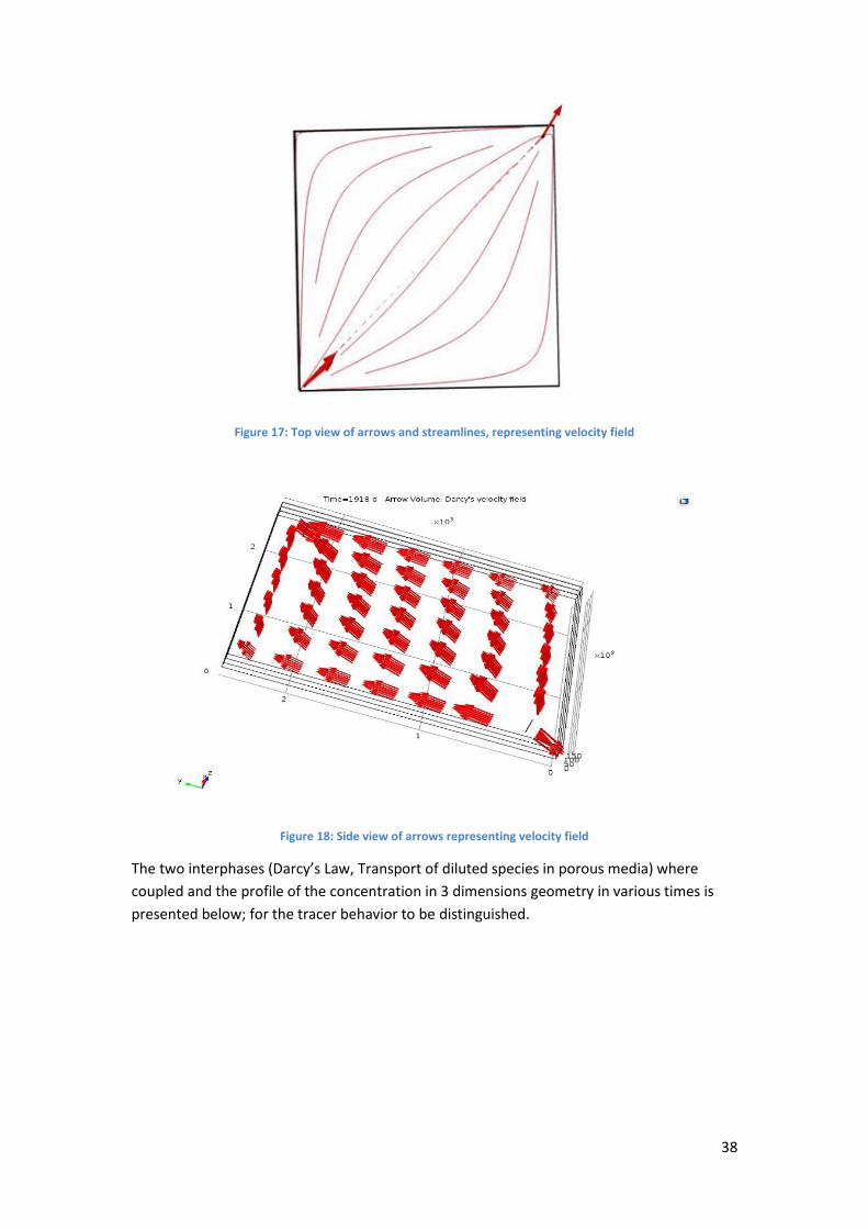
38
Figure 17: Top view of arrows and streamlines, representing velocity field
Figure 18: Side view of arrows representing velocity field
The two interphases (Darcy’s Law, Transport of diluted species in porous media) where
coupled and the profile of the concentration in 3 dimensions geometry in various times is
presented below; for the tracer behavior to be distinguished.

39
Figure 19: Contour concentration 3D graph; 14th
day of tracer’s injection
Figure 20: Injection well view at 203rd
day of injection.

40
Figure 21: Contour concentration 3D graph; 364th
day of tracer’s injection
Figure 22: Contour concentration 3D graph; 1001st
day of tracer’s injection
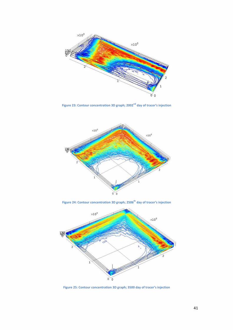
41
Figure 23: Contour concentration 3D graph; 2002nd
day of tracer’s injection
Figure 24: Contour concentration 3D graph; 2506th
day of tracer’s injection
Figure 25: Contour concentration 3D graph; 3500 day of tracer’s injection
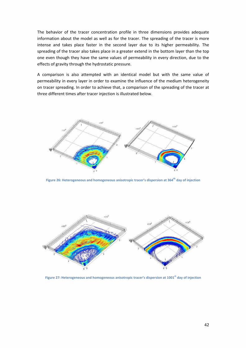
42
The behavior of the tracer concentration profile in three dimensions provides adequate
information about the model as well as for the tracer. The spreading of the tracer is more
intense and takes place faster in the second layer due to its higher permeability. The
spreading of the tracer also takes place in a greater extend in the bottom layer than the top
one even though they have the same values of permeability in every direction, due to the
effects of gravity through the hydrostatic pressure.
A comparison is also attempted with an identical model but with the same value of
permeability in every layer in order to examine the influence of the medium heterogeneity
on tracer spreading. In order to achieve that, a comparison of the spreading of the tracer at
three different times after tracer injection is illustrated below.
Figure 26: Heterogeneous and homogeneous anisotropic tracer’s dispersion at 364th
day of injection
Figure 27: Heterogeneous and homogeneous anisotropic tracer’s dispersion at 1001st
day of injection

43
Figure 28: Heterogeneous and homogeneous anisotropic tracer’s dispersion at 2506th
day of injection
From the contour plots above it can be distinct that the slug moves uniformly in the porous
media and the spreading is less intense in the case of the isotropic reservoir. Furthermore it
is obvious that in the second case the tracer moves faster as it reaches the production well
at earlier time and more quantity of the diluted is absorbed in the same period of
production. This further highlights the effects of macroscale heterogeneities and anisotropy
(besides pore scale velocity fields) on the hydrodynamic dispersion of diluted species. Such
upscaled geological features produce preferential pathways and enhance concentration
gradients, resulting in better mixing but also non-Gaussian tracer recovery curves due
varying residence times of the tracer in different permeability layers.
Two more graphs will be presented at the end of this section. Normal total flux (mol/s) that
is exiting the reservoir and the total quantity of mol that remains inside the reservoir during
its lifetime. The two graphs are also compared with the case of homogeneous anisotropy in
order for certain conclusions to be extracted.
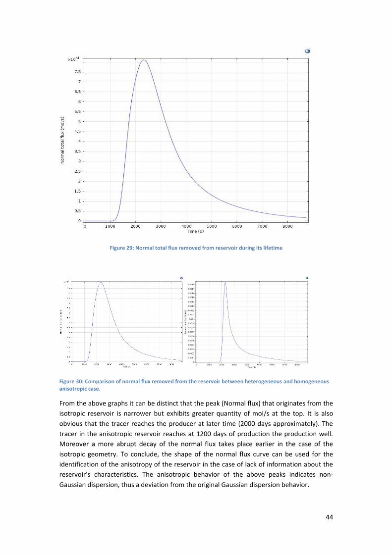
44
Figure 29: Normal total flux removed from reservoir during its lifetime
Figure 30: Comparison of normal flux removed from the reservoir between heterogeneous and homogeneous anisotropic case.
From the above graphs it can be distinct that the peak (Normal flux) that originates from the
isotropic reservoir is narrower but exhibits greater quantity of mol/s at the top. It is also
obvious that the tracer reaches the producer at later time (2000 days approximately). The
tracer in the anisotropic reservoir reaches at 1200 days of production the production well.
Moreover a more abrupt decay of the normal flux takes place earlier in the case of the
isotropic geometry. To conclude, the shape of the normal flux curve can be used for the
identification of the anisotropy of the reservoir in the case of lack of information about the
reservoir’s characteristics. The anisotropic behavior of the above peaks indicates non-
Gaussian dispersion, thus a deviation from the original Gaussian dispersion behavior.

45
Non-Gaussian dispersion features appear when transit times through some individual
heterogeneous structures become of the order of magnitude of the global transit time
through the whole sample. This might be the case when very large heterogeneities with a
moderate velocity contrasts with the rest of the sample are present (for instance in stratified
media); this is also the case for smaller heterogeneities with a very large velocity contrast (
for instance double-porosity packing of grains with a very low internal permeability acting as
a dead zones). In the second case, these features are not suppressed by a flow reversal but
give instead rise to both short and long time deviations from the Gaussian dispersion shapes.
(Wong, 1996)
Figure 31: Total quantity of moles that exist in the reservoir while production evolves
The two graphs below present the quantity of the tracer that is left inside the system in the
two cases of the isotropic and anisotropic reservoirs versus time; for the behavior of the
tracer during injection and production processes to be quantified. In this comparison small
differences occur between the two reservoirs. The total quantity of moles starts to decay
earlier in the case of anisotropy, and that points out that the tracer reaches earlier the
production well. The rate of decay of the Ntotal (moles) is similar in both cases and after
4000 days of production the quantity remaining in the system is the same.
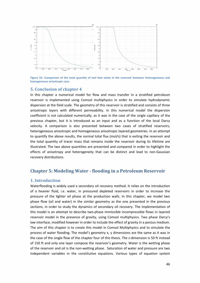
46
Figure 32: Comparison of the total quantity of mol that exists in the reservoir between heterogeneous and homogeneous anisotropic case.
5. Conclusion of chapter 4 In this chapter a numerical model for flow and mass transfer in a stratified petroleum
reservoir is implemented using Comsol multiphysics in order to simulate hydrodynamic
dispersion at the field scale. The geometry of this reservoir is stratified and consists of three
anisotropic layers with different permeability. In this numerical model the dispersion
coefficient is not calculated numerically, as it was in the case of the single capillary of the
previous chapter, but it is introduced as an input and as a function of the local Darcy
velocity. A comparison is also presented between two cases of stratified reservoirs;
heterogeneous anisotropic and homogeneous anisotropic layered geometries. In an attempt
to quantify the above results, the normal total flux (mol/s) that is exiting the reservoir and
the total quantity of tracer mass that remains inside the reservoir during its lifetime are
illustrated. The two above quantities are presented and compared in order to highlight the
effects of anisotropy and heterogeneity that can be distinct and lead to non-Gaussian
recovery distributions.
Chapter 5: Modeling Water - flooding in a Petroleum Reservoir
1. Introduction Waterflooding is widely used a secondary oil recovery method. It relies on the introduction
of a heavier fluid, i.e. water, in pressured depleted reservoirs in order to increase the
pressure of the lighter oil phase at the production walls. In this chapter, we model two
phase flow (oil and water) in the similar geometry as the one presented in the previous
sections, in order to study the dynamics of secondary oil recovery. The implementation of
this model is an attempt to describe two-phase immiscible incompressible flows in layered
reservoir model in the presence of gravity, using Comsol multiphysics. Two phase Darcy’s
law interface, modified however in order to include the effect of gravity in a porous medium.
The aim of this chapter is to create this model in Comsol Multiphysics and to simulate the
process of water flooding. The model’s geometry x, y dimensions are the same as it was in
the case of the single flow of the chapter four of this thesis. The z-dimension is 50 ft instead
of 150 ft and only one layer compose the reservoir’s geometry. Water is the wetting phase
of the reservoir and oil is the non-wetting phase. Saturation of water and pressure are two
independent variables in the constitutive equations. Various types of equation system

47
formulations for modelling two-phase flow in porous media using the finite element method
have been investigated. The system of equations consists of mass balances, partial
differential equations (PDEs) that describe the accumulation, transport and
injection/production of the phases in the model. In addition, several auxiliary equations (eg.
hydraulic properties) apply to the system, coupling the different phases in the system
together. This set of equations, PDEs and auxiliary equations, allows for equation
manipulation such that the main differences between the formulations are the dependent
variables that are solved for. Dependent variables of the PDE system are saturation of the
wetting phase and the pressure assuming negligible capillary pressure effects at the field
scale.
Firstly the pressure of the wetting phase is presented in order to identify if the model is
physically correct and if there is a variance of the pressure in three dimensions due to the
anisotropy of the reservoir. Then the change of saturation of the non-wetting phase due to
the injection of wetting phase in the reservoir can be identified. At the end of this section a
comparison is attempted with the commercial Eclipse software, which is commonly used in
oil recovery studies in order to compare the quality of the results between the two models.
2. Transport equations for fractional flow theory When two immiscible fluids with strong wettability preference are pumped
simultaneously through a porous medium, they tend to flow in separate channels and
maintain their identities, but with two miscible fluids no such experiment is possible.
Displacement in the case of immiscible fluids is generally not complete, but a fluid can be
displaced completely from the pores by another fluid that is miscible with it in all
proportions; that is, in the case of miscible fluids there are no residual saturations. In the
immiscible displacement process, neglecting capillarity results in the prediction of a sharp
front (step function) between the displacing and the displaced phases (Buckley-Leverett
profile). This situation is approached in reality when the flow rates are relatively high. At low
flow rates, the effect of capillarity results in a smearing of the saturation profile. In miscible
displacement there is no capillarity; instead there is mixing (Dispersion) of the two fluids. It
turns out that at relatively low flow rates the effect of dispersion is slight as compared with
the rate of advance of the displacing fluid. Hence, under these conditions, the approximation
of using sharp displacing font is often a good one. In the case of miscible displacement the
transition from pure displacing to pure displaced phase tends to become more gradual at
increasing flow rates. (Dullien, 1979)
The reservoir system to be modelled consists of a five-spot pattern of four production wells
surrounding each injection well. However, the symmetry of the system allows us to model a
single injection production pair, which will be located at opposite corners of a grid, as shown
in Figure 1. The system is initially at connate water saturation (Swc), and a water flood
calculation is to be performed to evaluate oil production and water breakthrough time. The
reservoir will be maintained above the bubble point pressure (Pb) at all times, and thus there
is no need to perform calculations for a free gas phase (in the reservoir). Reservoir and fluid
properties, such as layer permeabilities, porosity, oil and water densities and viscosities and
relative permeability data, are provided, as are the initial reservoir conditions and
production schedule was described.
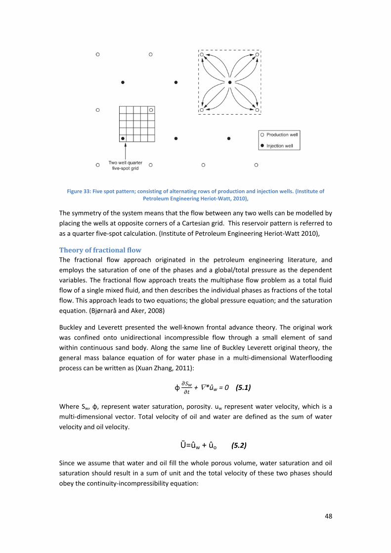
48
Figure 33: Five spot pattern; consisting of alternating rows of production and injection wells. (Institute of Petroleum Engineering Heriot-Watt, 2010),
The symmetry of the system means that the flow between any two wells can be modelled by
placing the wells at opposite corners of a Cartesian grid. This reservoir pattern is referred to
as a quarter five-spot calculation. (Institute of Petroleum Engineering Heriot-Watt 2010),
Theory of fractional flow
The fractional flow approach originated in the petroleum engineering literature, and
employs the saturation of one of the phases and a global/total pressure as the dependent
variables. The fractional flow approach treats the multiphase flow problem as a total fluid
flow of a single mixed fluid, and then describes the individual phases as fractions of the total
flow. This approach leads to two equations; the global pressure equation; and the saturation
equation. (Bjørnarå and Aker, 2008)
Buckley and Leverett presented the well-known frontal advance theory. The original work
was confined onto unidirectional incompressible flow through a small element of sand
within continuous sand body. Along the same line of Buckley Leverett original theory, the
general mass balance equation of for water phase in a multi-dimensional Waterflooding
process can be written as (Xuan Zhang, 2011):
φ 𝜕𝑆𝑤
𝜕𝑡 + *ûw = 0 (5.1)
Where Sw, φ, represent water saturation, porosity. uw represent water velocity, which is a
multi-dimensional vector. Total velocity of oil and water are defined as the sum of water
velocity and oil velocity.
Ū=ûw + ûo (5.2)
Since we assume that water and oil fill the whole porous volume, water saturation and oil
saturation should result in a sum of unit and the total velocity of these two phases should
obey the continuity-incompressibility equation:
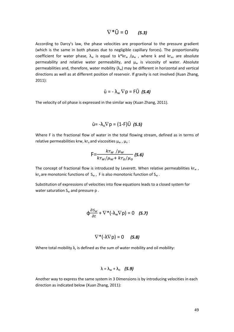
49
*Ū = 0 (5.3)
According to Darcy’s law, the phase velocities are proportional to the pressure gradient
(which is the same in both phases due to negligible capillary forces). The proportionality
coefficient for water phase, λw is equal to k*krw /μw , where k and krw, are absolute
permeability and relative water permeability, and μw is viscosity of water. Absolute
permeabilities and, therefore, water mobility (λw) may be different in horizontal and vertical
directions as well as at different position of reservoir. If gravity is not involved (Xuan Zhang,
2011):
ū = - λw p = FŪ (5.4)
The velocity of oil phase is expressed in the similar way (Xuan Zhang, 2011).
ū= -λοp = (1-F)Ū (5.5)
Where F is the fractional flow of water in the total flowing stream, defined as in terms of
relative permeabilities krw, kro and viscosities μw , μo :
F=𝑘𝑟𝑤 /𝜇𝑤
𝑘𝑟𝑤/𝜇𝑤+ 𝑘𝑟𝑜/𝜇𝑜 (5.6)
The concept of fractional flow is introduced by Leverett. When relative permeabilities krw ,
kro are monotonic functions of Sw , F is also monotonic function of Sw .
Substitution of expressions of velocities into flow equations leads to a closed system for
water saturation Sw and pressure p .
φ𝜕𝑆𝑤
𝜕𝑡 + *(-λwp) = 0 (5.7)
*(-λp) = 0 (5.8)
Where total mobility λ, is defined as the sum of water mobility and oil mobility:
λ = λw + λο (5.9)
Another way to express the same system in 3 Dimensions is by introducing velocities in each
direction as indicated below (Xuan Zhang, 2011):

50
ûwx = -λwx𝜕𝑃
𝜕𝑥 (5.10.1) ûnwx = -λnwx
𝜕𝑃
𝜕𝑥 (5.10.4)
ûwy = -λwy𝜕𝑃
𝜕𝑦 (5.10.2) ûnwy = -λnwy
𝜕𝑃
𝜕𝑦 (5.10.5)
ûwz = -λwz (𝜕𝑃
𝜕𝑧 - ρ*gg ) (5.10.3) ûnwz = -λnw(
𝜕𝑃
𝜕𝑧 - ρ*gg) (5.10.6)
The system equations (5.1) and (5.3) equations presented above can be rewritten for the
case of water flooding in three dimensions without the effect of gravity (Xuan Zhang, 2011) :
φ𝜕𝑆𝑤
𝜕𝑡 +
𝜕
𝜕𝑥(- λwx
𝜕𝑝
𝜕𝑥 ) +
𝜕
𝜕𝑦(- λwy
𝜕𝑝
𝜕𝑦) +
𝜕
𝜕𝑧[-λwz(
𝜕𝑝
𝜕𝑧 - ρ*gg)] = 0 (5.11)
𝜕
𝜕𝑥(λχ
𝜕𝑝
𝜕𝑥) +
𝜕
𝜕𝑦(λy
𝜕𝑝
𝜕𝑦) +
𝜕
𝜕𝑧[λz(
𝜕𝑝
𝜕𝑧 + ρ*gg)] = 0 (5.12)
The 3D water flooding system described by the two equations above aims to solve for water
saturation Sw, total pressure (P) and velocities ûx, ûy, ûz. These equations will be
implemented in COMSOL to simulate the process of 3D water flooding. Also relative
permeabilities (Krw and krnw) that are implemented inside the mobility λw and λnw are treated
as intermediate functions dependent on water saturation Sw. (Xuan Zhang, 2011)
If fluid or matrix compressibility is considered, then appropriate compressibility coefficients
also need to be defined. For the purposes of this case study all fluids, as well as the solid
matrix, will be considered to be incompressible. Given this set of equations, boundary and
initial conditions must be supplied to complete the mathematical description. These are
usually given as known pressures, saturations or fluxes in each of the fluid phases. An
important criterion for acceptance of a numerical method is that it must be able to solve the
governing equations for the wide variety of possible boundary conditions. (Binning, and
Celia, 1998)
Darcy’s Equation for Two-phase flow
Two-phase Darcy interface uses the same equations with Darcy’s but for two fluids. The
implementation of the equations of the Comsol follows the fractional flow theory. A total
pressure is utilized instead of two pressures, one for each wetting phase. The fractional flow
theory, calculate the individual phases as fractions of the total flow. In addition, weighted
averages equations are used for the description of the total density and total viscosity at
each timestep. Since the saturation of each fluid is constantly changing, so is the
contribution of each fluid density and each fluid viscosity. The weighted averages equations
are utilized in order to simulate the compressibility of the fluids. Moreover the sum of two
saturations set to be equal to unity. Finally an altered saturation equation is utilized with the
use of c1 coefficient. The two dependent variables are global pressure and c1 coefficient,
function of saturation S1. The exact equations, this interface utilizes are presented next.
𝜕𝑒𝑝𝜌
𝜕𝑡 + *ρu =0 (5.13), u = -
𝑘
𝜇*p
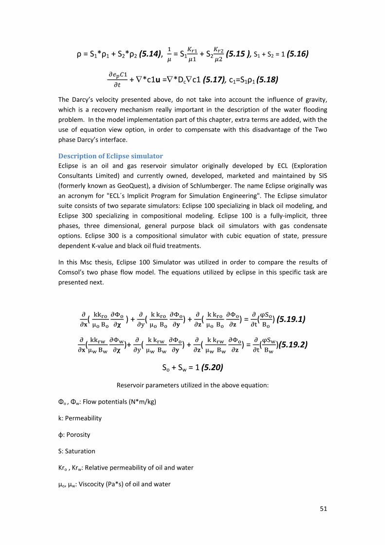
51
ρ = S1*ρ1 + S2*ρ2 (5.14), 1
𝜇 = S1
𝐾𝑟1
𝜇1 + S2
𝐾𝑟2
𝜇2 (5.15 ), S1 + S2 = 1 (5.16)
𝜕𝑒𝑝𝐶1
𝜕𝑡 + *c1u =*Dcc1 (5.17), c1=S1ρ1 (5.18)
The Darcy’s velocity presented above, do not take into account the influence of gravity,
which is a recovery mechanism really important in the description of the water flooding
problem. In the model implementation part of this chapter, extra terms are added, with the
use of equation view option, in order to compensate with this disadvantage of the Two
phase Darcy’s interface.
Description of Eclipse simulator
Eclipse is an oil and gas reservoir simulator originally developed by ECL (Exploration
Consultants Limited) and currently owned, developed, marketed and maintained by SIS
(formerly known as GeoQuest), a division of Schlumberger. The name Eclipse originally was
an acronym for "ECL´s Implicit Program for Simulation Engineering". The Eclipse simulator
suite consists of two separate simulators: Eclipse 100 specializing in black oil modeling, and
Eclipse 300 specializing in compositional modeling. Eclipse 100 is a fully-implicit, three
phases, three dimensional, general purpose black oil simulators with gas condensate
options. Eclipse 300 is a compositional simulator with cubic equation of state, pressure
dependent K-value and black oil fluid treatments.
In this Msc thesis, Eclipse 100 Simulator was utilized in order to compare the results of
Comsol’s two phase flow model. The equations utilized by eclipse in this specific task are
presented next.
∂
∂𝐱(
kkro
μo Bo
∂Φo
∂𝛘 ) +
∂
∂y(
k kro
μo Bo ∂Φο
∂𝐲) +
∂
∂𝐳(
k kro
μo Bo ∂Φο
∂𝐳) =
∂
∂t(φSo
Bo) (5.19.1)
∂
∂𝐱(
kkrw
μw Bw
∂Φw
∂𝛘)+
∂
∂y(
k krw
μw Bw ∂Φο
∂𝐲) +
∂
∂𝐳(
k krw
μw Bw ∂Φο
∂𝐳) =
∂
∂t(φSw
Bw)(5.19.2)
So + Sw = 1 (5.20)
Reservoir parameters utilized in the above equation:
Φo , Φw: Flow potentials (N*m/kg)
k: Permeability
φ: Porosity
S: Saturation
Kro , Krw: Relative permeability of oil and water
μo, μw: Viscocity (Pa*s) of oil and water

52
Bo, Bw: formation volume factor of each phase (RBBL/STB )
The equations (5.19.1), (5.19.2) presented above are solved in each grid block with the use
of finite differences method.(Schlumberger 2012)
3. Model Implementation in Comsol Multiphysics In the Chapter 5, two equations; the global pressure equation; and the saturation equation
are implemented in Comsol with the use of the Two phase Darcy’s law interface. The
equations can be found by adding the mass balances and do some numerical manipulation
for the pressure equation, and by subtracting the mass balances and some numerical
manipulation for the saturation equation. Furthermore, the differential equations need to
be solved together with a set of boundary conditions.
These equations are solved together as a time dependent problem for 2000 days at 1 day
intervals. As Mesh settings sequence type is selected to be Physics controlled - mesh and the
element size is set to be fine.
As a first step to build the model in Comsol Multiphysics the geometry of the three
dimensional porous media is implemented.
Figure 34: Geometry of the two phase flow reservoir
The reservoir geometry is similar with the one that was used in chapter four. The size of the
reservoir is 2500’x2500’x50’ and it consists of only one anisotropic layer. The only difference
is in z-dimension’s length and the total size of the reservoir is three times less than the
previous case. Two wells are placed in the same location as it was in the single fluid flow
case, one injection well and one production well with a radius of 10 ft each.
The mechanism than controls the secondary recovery of the reservoir is the flow of water
from the injection well, and can be identified with the change of saturation of the wetting
phase.
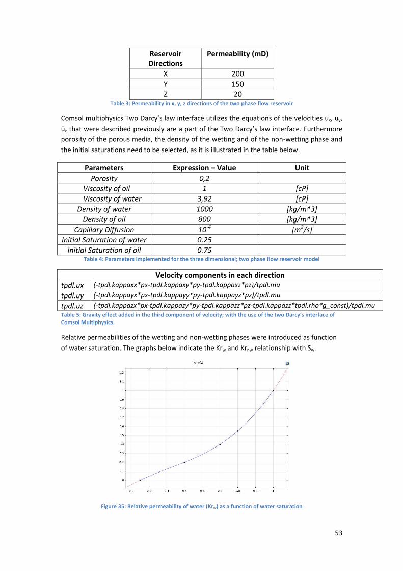
53
Reservoir Directions
Permeability (mD)
X 200
Y 150
Z 20 Table 3: Permeability in x, y, z directions of the two phase flow reservoir
Comsol multiphysics Two Darcy’s law interface utilizes the equations of the velocities ūx, ūy,
ūz that were described previously are a part of the Two Darcy’s law interface. Furthermore
porosity of the porous media, the density of the wetting and of the non-wetting phase and
the initial saturations need to be selected, as it is illustrated in the table below.
Parameters Expression – Value Unit
Porosity 0,2
Viscosity of oil 1 [cP]
Viscosity of water 3,92 [cP]
Density of water 1000 [kg/m^3]
Density of oil 800 [kg/m^3]
Capillary Diffusion 10-4 [m2/s]
Initial Saturation of water 0.25
Initial Saturation of oil 0.75 Table 4: Parameters implemented for the three dimensional; two phase flow reservoir model
Velocity components in each direction tpdl.ux (-tpdl.kappaxx*px-tpdl.kappaxy*py-tpdl.kappaxz*pz)/tpdl.mu
tpdl.uy (-tpdl.kappayx*px-tpdl.kappayy*py-tpdl.kappayz*pz)/tpdl.mu
tpdl.uz (-tpdl.kappazx*px-tpdl.kappazy*py-tpdl.kappazz*pz-tpdl.kappazz*tpdl.rho*g_const)/tpdl.mu Table 5: Gravity effect added in the third component of velocity; with the use of the two Darcy’s interface of Comsol Multiphysics.
Relative permeabilities of the wetting and non-wetting phases were introduced as function
of water saturation. The graphs below indicate the Krw and Krnw relationship with Sw.
Figure 35: Relative permeability of water (Krw) as a function of water saturation
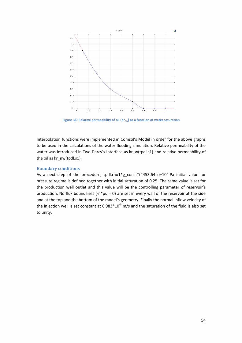
54
Figure 36: Relative permeability of oil (Krnw) as a function of water saturation
Interpolation functions were implemented in Comsol’s Model in order for the above graphs
to be used in the calculations of the water flooding simulation. Relative permeability of the
water was introduced in Two Darcy’s interface as kr_w(tpdl.s1) and relative permeability of
the oil as kr_nw(tpdl.s1).
Boundary conditions
As a next step of the procedure, tpdl.rho1*g_const*(2453.64-z)+105 Pa initial value for
pressure regime is defined together with initial saturation of 0.25. The same value is set for
the production well outlet and this value will be the controlling parameter of reservoir’s
production. No flux boundaries (-n*ρu = 0) are set in every wall of the reservoir at the side
and at the top and the bottom of the model’s geometry. Finally the normal inflow velocity of
the injection well is set constant at 6.983*10-5 m/s and the saturation of the fluid is also set
to unity.

55
Figure 37: Fine element size – Mesh selected in 3D Geometry model.
The above mesh sequence physics control option was selected and the size of the element
was selected to be fine. It can be distinct that in the area around the wells the element size
is even finer in order for the simulation to be more detailed in those areas.
4. Results & Discussion In Figures 38-40, we present the streamlines and wetting phase velocity arrows. As
expected, the flow of the wetting phase is from the inlet to the production well, with higher
velocities observed closer to the wells where there is limited space for flow. Accordingly the
pressure profiles of figures 44 - 47, show the dynamics of water pressure with higher
pressures closer to the injection well and closer to the bottom of the reservoir due to
hydrostatic pressure. Furthermore, saturations of the wetting and non-wetting phase are
presented in order to identify the impact of the secondary recovery process in the
production of oil. Moreover, Stock Tank Barrels/day of oil that are produced, and bottom
hole pressure (Pa) of injection and production well are presented. Finally a comparison with
the results of the Eclipse simulator is attempted, in order to evaluate Comsol’s multiphysics
model.

56
Figure 38: Streamlines in two phase flow simulation; representing velocity field
Figure 39: Streamlines in two phase flow simulation; representing velocity field
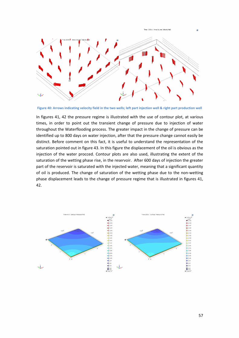
57
Figure 40: Arrows indicating velocity field in the two wells; left part injection well & right part production well
In figures 41, 42 the pressure regime is illustrated with the use of contour plot, at various
times, in order to point out the transient change of pressure due to injection of water
throughout the Waterflooding process. The greater impact in the change of pressure can be
identified up to 800 days on water injection, after that the pressure change cannot easily be
distinct. Before comment on this fact, it is useful to understand the representation of the
saturation pointed out in figure 43. In this figure the displacement of the oil is obvious as the
injection of the water procced. Contour plots are also used, illustrating the extent of the
saturation of the wetting phase rise, in the reservoir. After 600 days of injection the greater
part of the reservoir is saturated with the injected water, meaning that a significant quantity
of oil is produced. The change of saturation of the wetting phase due to the non-wetting
phase displacement leads to the change of pressure regime that is illustrated in figures 41,
42.

58
Figure 41: Pressure regime in two phase flow simulation at 0 to 600 days of injection
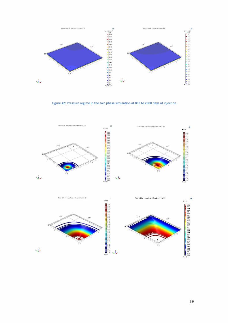
59
Figure 42: Pressure regime in the two phase simulation at 800 to 2000 days of injection
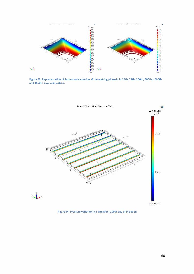
60
Figure 43: Representation of Saturation evolution of the wetting phase in in 25th, 75th, 200th, 600th, 1000th and 1600th days of injection.
Figure 44: Pressure variation in z direction; 200th day of injection
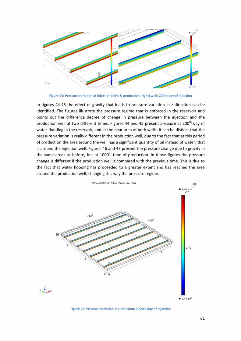
61
Figure 45: Pressure variation at injection (left) & production (right) well; 200th day of injection
In figures 44-48 the effect of gravity that leads to pressure variation in z direction can be
identified. The figures illustrate the pressure regime that is enforced in the reservoir and
points out the difference degree of change in pressure between the injection and the
production well at two different times. Figures 44 and 45 present pressure at 200th day of
water-flooding in the reservoir, and at the near area of both wells. It can be distinct that the
pressure variation is really different in the production well, due to the fact that at this period
of production the area around the well has a significant quantity of oil instead of water; that
is around the injection well. Figures 46 and 47 present the pressure change due to gravity in
the same areas as before, but at 1000th time of production. In those figures the pressure
change is different if the production well is compared with the previous time. This is due to
the fact that water flooding has proceeded to a greater extent and has reached the area
around the production well; changing this way the pressure regime.
Figure 46: Pressure variation in z direction; 1000th day of injection
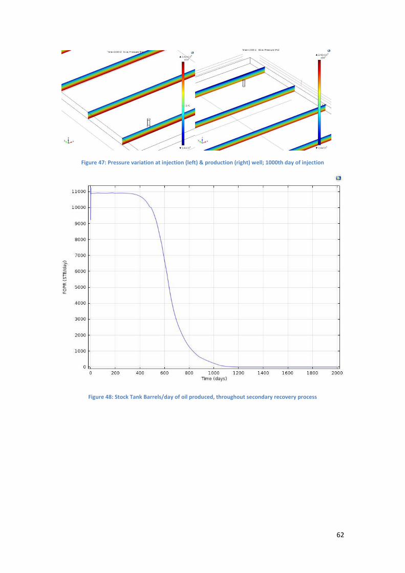
62
Figure 47: Pressure variation at injection (left) & production (right) well; 1000th day of injection
Figure 48: Stock Tank Barrels/day of oil produced, throughout secondary recovery process

63
Figure 49: Stock Tank Barrels/day of water produced, throughout secondary recovery process
In Figure 48 the Stock Tank Barrels/day of oil that are produced at water-flooding process.
After a few days the production rate reaches a plateau, at about 3400 STB/day, until 600
days of injection. From this time and on, the production rate starts decaying smoothly until
the end of reservoir’s life; after 2000 days of production. Since the bottom hole pressure is
set constant in order to control the production of oil, the production rate reaches a plateau
until a point where the bottom hole pressure cannot sustain this production rate.
In figure 49 the Stock Tank Barrels/day of water that are produced at water injection process
are presented. Water production is zero at the start of production; since the initial
saturation of 0.25 indicates the irreducible quantity of water, which is immobile. After 600
days of production the water production starts rising due to the fact that the injected water
has reached the area around the production well. From this point and on, the quantity of
water produced continue rising until the end of reservoir’s production.
In figures 50 and 51 bottom hole pressure of injection well and the average reservoir
pressure are presented throughout the secondary recovery process. The pressure of the
production well is set constant at 2.407 * 107 Pa. The injection well bottom hole pressure is
increasing and reaches a maximum after approximately 600 days of production. This effect
has to do with the increasing quantity of water that is introduced in the reservoir. Since a
quantity of oil is removed at the same time that water is injected in the system, after some
point due to the quantity of fluids that are removed the pressure starts decaying. The decay
of the pressure appears after approximately 600 days until the end of reservoir’s production

64
at the 2000th day. The average reservoir pressure starts rising from a value of 2.413 * 107 Pa.
Pressure of the system, due to water injection, is increasing and reaches a peak at 600 days
of production. From this point and on, the average reservoir pressure starts to decline until
the end of reservoir’s life, due to the change in average viscosity of the reservoir.
Figure 50: Bottom Hole Pressure of injection & production well throughout waterflood process
Figure 51: Average Reservoir Pressure throughout waterflood process
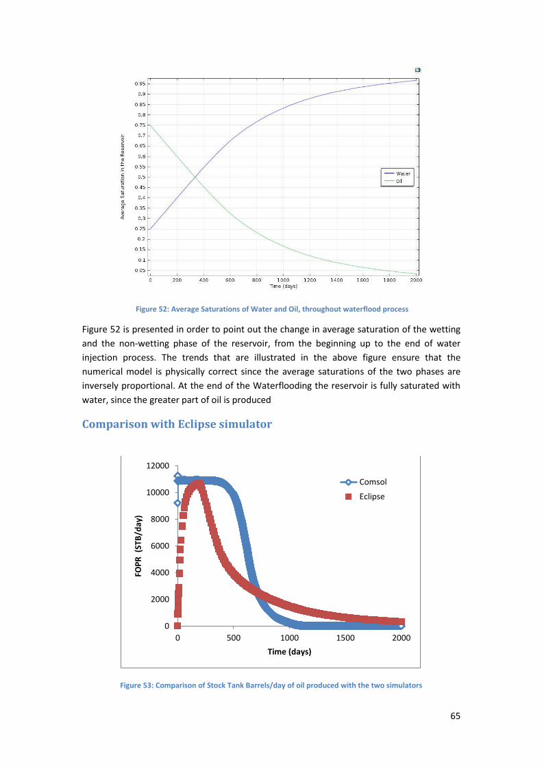
65
Figure 52: Average Saturations of Water and Oil, throughout waterflood process
Figure 52 is presented in order to point out the change in average saturation of the wetting
and the non-wetting phase of the reservoir, from the beginning up to the end of water
injection process. The trends that are illustrated in the above figure ensure that the
numerical model is physically correct since the average saturations of the two phases are
inversely proportional. At the end of the Waterflooding the reservoir is fully saturated with
water, since the greater part of oil is produced
Comparison with Eclipse simulator
Figure 53: Comparison of Stock Tank Barrels/day of oil produced with the two simulators
0
2000
4000
6000
8000
10000
12000
0 500 1000 1500 2000
FOP
R (
STB
/day
)
Time (days)
Comsol
Eclipse
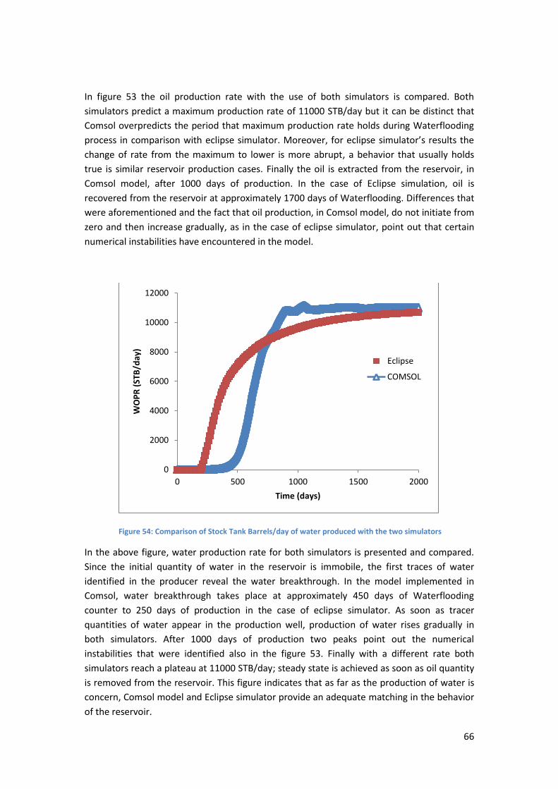
66
In figure 53 the oil production rate with the use of both simulators is compared. Both
simulators predict a maximum production rate of 11000 STB/day but it can be distinct that
Comsol overpredicts the period that maximum production rate holds during Waterflooding
process in comparison with eclipse simulator. Moreover, for eclipse simulator’s results the
change of rate from the maximum to lower is more abrupt, a behavior that usually holds
true is similar reservoir production cases. Finally the oil is extracted from the reservoir, in
Comsol model, after 1000 days of production. In the case of Eclipse simulation, oil is
recovered from the reservoir at approximately 1700 days of Waterflooding. Differences that
were aforementioned and the fact that oil production, in Comsol model, do not initiate from
zero and then increase gradually, as in the case of eclipse simulator, point out that certain
numerical instabilities have encountered in the model.
Figure 54: Comparison of Stock Tank Barrels/day of water produced with the two simulators
In the above figure, water production rate for both simulators is presented and compared.
Since the initial quantity of water in the reservoir is immobile, the first traces of water
identified in the producer reveal the water breakthrough. In the model implemented in
Comsol, water breakthrough takes place at approximately 450 days of Waterflooding
counter to 250 days of production in the case of eclipse simulator. As soon as tracer
quantities of water appear in the production well, production of water rises gradually in
both simulators. After 1000 days of production two peaks point out the numerical
instabilities that were identified also in the figure 53. Finally with a different rate both
simulators reach a plateau at 11000 STB/day; steady state is achieved as soon as oil quantity
is removed from the reservoir. This figure indicates that as far as the production of water is
concern, Comsol model and Eclipse simulator provide an adequate matching in the behavior
of the reservoir.
0
2000
4000
6000
8000
10000
12000
0 500 1000 1500 2000
WO
PR
(ST
B/d
ay)
Time (days)
Eclipse
COMSOL
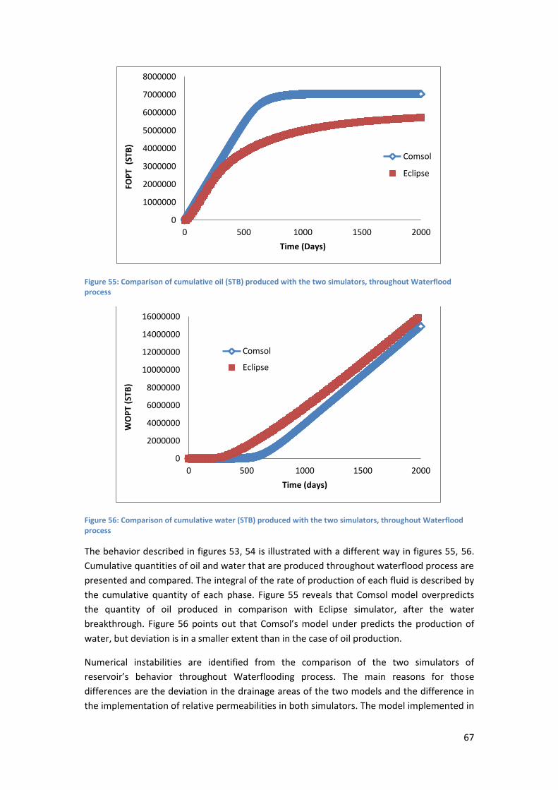
67
Figure 55: Comparison of cumulative oil (STB) produced with the two simulators, throughout Waterflood process
Figure 56: Comparison of cumulative water (STB) produced with the two simulators, throughout Waterflood process
The behavior described in figures 53, 54 is illustrated with a different way in figures 55, 56.
Cumulative quantities of oil and water that are produced throughout waterflood process are
presented and compared. The integral of the rate of production of each fluid is described by
the cumulative quantity of each phase. Figure 55 reveals that Comsol model overpredicts
the quantity of oil produced in comparison with Eclipse simulator, after the water
breakthrough. Figure 56 points out that Comsol’s model under predicts the production of
water, but deviation is in a smaller extent than in the case of oil production.
Numerical instabilities are identified from the comparison of the two simulators of
reservoir’s behavior throughout Waterflooding process. The main reasons for those
differences are the deviation in the drainage areas of the two models and the difference in
the implementation of relative permeabilities in both simulators. The model implemented in
0
1000000
2000000
3000000
4000000
5000000
6000000
7000000
8000000
0 500 1000 1500 2000
FOP
T (
STB
)
Time (Days)
Comsol
Eclipse
0
2000000
4000000
6000000
8000000
10000000
12000000
14000000
16000000
0 500 1000 1500 2000
WO
PT
(STB
)
Time (days)
Comsol
Eclipse
68
Comsol multiphysics describes the production and the injection wells as cylinders with a
radius of 10 ft and a height of 50 ft. The boundaries of each cylinder, is selected as the inlet
and the outlet of the reservoir’s water injection process. The inflow of 11000 STB/days of
water injected, is introduced as an inlet velocity and is adjusted to the area of the cylinder in
order to have identical conditions with the injection well of the model that eclipse simulator
utilizes; Eclipse uses in both wells a point source for production and injection wells. In the
case of production well the outlet conditions applied, and thus the controlling mechanism of
production is a constant pressure. Due to the fact that the production is controlled by a
constant value of pressure, the rate of production cannot be controlled and that results to
an area around the production well with deviations between the two models. In figures 35 &
36 the relative permeabilities krw and krnw, as functions of water saturation, of the two
phases that were introduced in Comsol’s model are presented. In addition equation (5.12)
describes the way that relative permeability is introduced in Comsol’s numerical model,
through average viscosity of the total fluid which is changing as the saturation of water is
rising. On the other hand, equations (5.19.1) and (5.19.2) describe the way that relative
permeabilities are introduced in the three dimensions of the reservoir in eclipse simulator. It
is obvious from the results extracted that numerical instabilities can be identified also at the
initial and at the final values of saturations at the edges of relative permeabilities functions.
This behavior leads to the conclusion that the extrapolation out of the relative
permeabilities range is unstable.
The equations (PDEs) that are utilized in Comsol multiphysics are a realization of fractional
flow theory. Fractional flow treats the multiphase flow problem as a total fluid flow of a
single mixed fluid, and then describes the individual phases as fractions of the total flow.
This approach and the fact that Comsol cannot identify the immobile quantities of each
phase, since it address the two phase flow as a single phase flow simulation problem, leads
to uncertainties about the quality of the results extracted. On the contrary, spatial resolution
(Mesh instead of grid) and time stepping are finer in Comsol multiphysics and thus there is a
more detailed description of the solution. Nevertheless, as a result of the geometry of the
problem the grid orientation effect arises when Eclipse simulator is utilized. This
phenomenon is particularly severe in reservoir simulation and in certain cases it can increase
substantially the uncertainty of the numerical predictions. In the grid geometry that is used
in eclipse simulator, there is fluid flow oriented with diagonally across the grid. If the two
wells were oriented with the principal grid direction the results of the simulation would be
different. This can produce simulations for two phase flows with unphysical results. In
Comsol multiphysics the use of triangular mesh and the fact that the problem is solved
continuously; the orientation effect is avoided.
Moreover Comsol software is equipped with a graphical interface to use when the numerical
model is implemented. The PDES that are solved to describe the physical problem can be
identified and the user can interfere and implement a change if it is a necessity for the
problem. In the case of the two phase flow problem, the Two-Darcy’s interface did not
include the effect of gravity. In order for the numerical model to be consistent with the
physical reality of Waterflooding process, additional terms were added in the PDEs that
Comsol utilizes. Eclipse simulator uses finite differences method to solve the PDEs of the
problem and Taylor’s expansion for the approximation of the derivatives. Comsol
69
Multiphysics uses finite elements method; reduces the number of unknowns and thus the
complexity of the simulation. To conclude, eclipse utilizes more precise description of the
reservoir simulation problem, since it uses different equation for each phase and Comsol
utilizes a single equation and time dependent average quantities of density (ρ) and viscosity
(μ) and the saturation of the wetting phase, as a dependent variable. The way that the PDEs
are solved in time and in space is more detailed in Comsol multiphysics and cost less in
computation time; advantage in comparison with Eclipse reservoir simulation software.
5. Conclusion of chapter 5 A numerical model for two-phase flow under gravity was implemented in Comsol
Multiphysics in order to simulate process of water flooding during secondary oil recovery in
heterogeneous and anisotropic three dimensional reservoirs. In the above model relative
permeabilities of the wetting and non-wetting phase were introduced as functions of water
saturation (Sw). The purpose of this study is to obtain information about the production rate
in STB/day of oil and water that are produced during the entire lifetime of the reservoir. The
effects of gravity on pressure dynamics are then illustrated in two different times for the
reservoir and in the area around the two wells, as the oil saturation changes locally towards
smaller values. The calculated values of bottom hole pressure for the injection well indicates
that pressure is increasing up to a maximum value and then starts decreasing until water
breakthrough takes place at the production well of the reservoir. At the end of this chapter
the results obtained from Comsol’s numerical model are compared with those of the Eclipse
simulator for the same reservoir simulation problem. The general response of the reservoir
is described adequately from both simulators, in terms of both oil recovery rates and
cumulative recovery. While in general good agreement, the numerical predictions of the
two models also exhibit distinct differences that should be attributed to the numerical
scheme used to solve the PDE’s and the effects of discretization, rather than the underlying
physical model, which is essentially the same in both cases. This particular point however
deserves further investigation in a future study.
Conclusions of Msc thesis Three numerical models were implemented in Comsol multiphysics in order to model single
and multi-phase flows in petroleum reservoirs. Firstly the effect of hydrodynamic dispersion
arising in the pore scale is reproduced. The influence of the parabolic pore scale velocity
profile in hydrodynamic dispersion coefficient in contrast to the flat velocity profile is
identified. Next hydrodynamic dispersion at a three dimensional reservoir is modeled, in an
attempted to point out pore to field-scale impact. Heterogeneous anisotropic and
homogeneous anisotropic layered reservoirs geometries are under the scope of this thesis,
and a comparison between non-Gaussian recovery distributions is illustrated in figures 30 &
32. In the last numerical model two-phase flow under the presence of gravity, simulate the
secondary recovery process of water-flooding in a homogeneous anisotropic reservoir.
Results of the change in pressure regime and in saturation are presented in figures 41, 42 &
43. As a last step, a comparison with the results of Eclipse reservoir simulator (53-56 figures)

70
is attempted to evaluate the possibility of whether Comsol Multiphysics can reproduce the
oil & water production rates provided by the widely used software of the oil industry.
Comsol Multiphysics 5.0 simulate successfully all three numerical models pointing out that
pore scale effects such as hydrodynamic dispersion determine the field scale transport
properties. A comparison of the two reservoir simulation models present acceptable
matching; indicating that Comsol multiphysics can be used as a reservoir simulation
alternative for the oil industry.
As a recommendation for future work, simulation of Waterflooding process in a stratified
geometry could be implemented in Comsol multiphysics and a comparison could again be
attempted with Eclipse simulator of Schlumberger, for the same reservoir simulation
problem.
References
Bear, J. (1972) Dynamics of fluids in Porous Media. New York: Dover
Publications
Bear, J. (1979) Hydraulics of Groundwater, New York: McGraw-Hill
Bear, J., & Bachmat, Y. (1967) A generalized theory on hydrodynamic
dispersion, Proc. I.A.S.H. Symposium on Artificial Recharge and
Management of Aquifers, IASH Publ.
Binning, P. & Celia, M.A. (1998) Practical implementation of the
fractional flow approach to multi-phase flow simulation. Advances in
Water Resources Vol. 22, No. 5
Bjørnarå, T. I. & Aker, E. (2008) Comparing Equations for Two-Phase
Fluid Flow in Porous Media, COMSOL Conference 2008 Hannover
COMSOL (2013).COMSOL Multiphysics, 4.3b Reference Manual. Version
COMSOL 4.3b .
COMSOL (2013).COMSOL Multiphysics, 4.3b Subsurface Flow Module
User’s Guide. Version COMSOL 4.3b .
COMSOL Multiphysics 2015. PDE equations. Available from:
<http://www.comsol.com/multiphysics/navier-stokes-equations>.[10
july 2015]

71
COMSOL Multiphysics 2015.Longitudinal and Transverse
dispersivity.Available from: <https://www.comsol.eu/model/effective-
diffusivity-in-porous-materials-978>.[30 july 2015]
Dullien, F.A.L. (1979) Porous Media: Fluid Transport and Pore Structure.
California: Elsevier Science
Green, D. W. & Willhite, G. P. (1998). Enhanced Oil Recovery, Society of
Petroleum Engineers.
Huebner, K. H. (2001) The Finite Element Method for Engineers, 4th ed.
New York: Wiley
Institute of Petroleum Engineering Heriot-Watt (2010), Heriot-Watt
University - Reservoir Simulation. Edinburgh: Heriot-Watt University
Liu, G. R. (2003) Finite Element Method a Practical Course. Oxford:
Butterworth-Heinemann
Maghsood, A.D., & Brigham, W.E. (1982) Analysis of unit Mobility Ratio
Well to Well tracer flow to determine reservoir heterogeneity. California:
Stanford University Petroleum Research Institute
Nunge, R. J. & Gill, W. N. (1969) Mechanisms Affecting Dispersion and
Miscible Displacement. Flow through porous media symposium Vol 61
No 9
Schlumberger 2012. Eclipse Technical Description* reservoir simulation
software. Version 2010.2 ed.
Schlumberger (2006). Reservoir Simulation Application Training Course
and (Eclipse) Workshop. Denver and Houston: Schlumberger
Wong, P. Z. (1996) Methods of the Physics of Porous Media. San Diego:
Elsevier Science
Xuan Zhang, S 2011, Upscaling of the Two-Phase Flows in Petroleum
Reservoirs. Ph.D. Thesis, Technical University of Denmark
Zemel, B. (1995) tracers in the oil field. Amsterdam: Elsevier Science
Related Documents