Modeling Simple Amphiphilic Solutes in a Jagla Solvent

Modeling simple amphiphilic solutes in a Jagla solventZhiqiang Su, Sergey V. Buldyrev, Pablo G. Debenedetti, Peter J. Rossky, and H. Eugene Stanley Citation: J. Chem. Phys. 136, 044511 (2012); doi: 10.1063/1.3677185 View online: http://dx.doi.org/10.1063/1.3677185 View Table of Contents: http://jcp.aip.org/resource/1/JCPSA6/v136/i4 Published by the American Institute of Physics. Related ArticlesMonte Carlo predictions of phase equilibria and structure for dimethyl ether + sulfur dioxide and dimethyl ether +carbon dioxide J. Chem. Phys. 136, 044514 (2012) Reorientation dynamics of nanoconfined water: Power-law decay, hydrogen-bond jumps, and test of a two-statemodel J. Chem. Phys. 136, 044513 (2012) Transport coefficients of the TIP4P-2005 water model J. Chem. Phys. 136, 044507 (2012) Monte Carlo study of four dimensional binary hard hypersphere mixtures J. Chem. Phys. 136, 014506 (2012) Energy relaxation of intermolecular motions in supercooled water and ice: A molecular dynamics study J. Chem. Phys. 135, 244511 (2011) Additional information on J. Chem. Phys.Journal Homepage: http://jcp.aip.org/ Journal Information: http://jcp.aip.org/about/about_the_journal Top downloads: http://jcp.aip.org/features/most_downloaded Information for Authors: http://jcp.aip.org/authors

THE JOURNAL OF CHEMICAL PHYSICS 136, 044511 (2012)

Modeling simple amphiphilic solutes in a Jagla solventZhiqiang Su,1,a) Sergey V. Buldyrev,1,2 Pablo G. Debenedetti,3 Peter J. Rossky,4

and H. Eugene Stanley1

1Center for Polymer Studies and Department of Physics, Boston University, Boston, Massachusetts 02215, USA2Department of Physics, Yeshiva University, 500 West 185th Street, New York, New York 10033, USA3Department of Chemical and Biological Engineering, Princeton University, Princeton,New Jersey 08544, USA4Department of Chemistry and Biochemistry, College of Natural Science, The University of Texas at Austin,Austin, Texas 78712, USA

(Received 7 September 2011; accepted 24 December 2011; published online 25 January 2012)

Methanol is an amphiphilic solute whose aqueous solutions exhibit distinctive physical properties.The volume change upon mixing, for example, is negative across the entire composition range, indi-cating strong association. We explore the corresponding behavior of a Jagla solvent, which has beenpreviously shown to exhibit many of the anomalous properties of water. We consider two models ofan amphiphilic solute: (i) a “dimer” model, which consists of one hydrophobic hard sphere linkedto a Jagla particle with a permanent bond, and (ii) a “monomer” model, which is a limiting case ofthe dimer, formed by concentrically overlapping a hard sphere and a Jagla particle. Using discretemolecular dynamics, we calculate the thermodynamic properties of the resulting solutions. We sys-tematically vary the set of parameters of the dimer and monomer models and find that one can readilyreproduce the experimental behavior of the excess volume of the methanol-water system as a functionof methanol volume fraction. We compare the pressure and temperature dependence of the excessvolume and the excess enthalpy of both models with experimental data on methanol-water solutionsand find qualitative agreement in most cases. We also investigate the solute effect on the temperatureof maximum density and find that the effect of concentration is orders of magnitude stronger thanmeasured experimentally. © 2012 American Institute of Physics. [doi:10.1063/1.3677185]

I. INTRODUCTION

Aqueous solutions of alcohol are important and ubiq-uitous in the medical, personal care, transportation (e.g.,antifreeze, fuels), and food industries, among others, andthus have attracted much theoretical and experimentalattention.1–11 Methanol is a simple example of an amphiphilicorganic solute, and its aqueous solutions exhibit many inter-esting nonidealities. Understanding this simple case is there-fore a natural starting point when studying more complex so-lutes in water, such as higher alcohols or proteins.

Because of the increasing availability of expanded com-puting power, simulations have become an important researchtool in studying aqueous methanol solutions.12, 24–29 The op-timized potential for liquid simulation13 is frequently usedto model alcohol molecules. To represent water as a solvent,the SPC/E,14 TIP3P,15 TIP4P,16 and TIP5P17 models are fre-quently used. Coarse-grained potentials also have been usedto explore the properties of water, e.g., the two-dimensional18

and three-dimensional19 Mercededes-Benz (MB) models,which have also provided many insights into the physics of thehydrogen-bond local structure of water and the hydrophobiceffect.18, 20–23

Recently, it was found that many thermodynamic prop-erties of water can be reproduced using soft-core sphericallysymmetric potentials, one of the most important of which is

a)Author to whom correspondence should be addressed. Electronic mail:[email protected].

the Jagla model.30 The Jagla potential has a hard core and alinear repulsive ramp, and contains two characteristic lengthscales: a hard core a and a soft core b. For a range of parame-ters, the Jagla model exhibits a water-like31 cascade of struc-tural, transport, and thermodynamic anomalies.30, 32, 33, 35, 36

Buldyrev et al. in 2007 (Ref. 37) found that the Jagla sol-vent exhibits key water-like characteristics with respect to hy-drophobic hydration, suggesting that the water-like character-istics of the Jagla solvent extend beyond the pure fluid.

In our coarse-grained model of solvent we have spheri-cally symmetric particles that do not have hydrogen clouds. Inthis sense, our model is simpler than the MB model, but it stillaccurately shows the trends for the hydrophobic effect of non-polar components. In our model, the tetrahedral anisotropy ofthe hydrogen bond is replaced by the repulsive ramp of theJagla particle, which makes the coordination number of themodel lower than that of the Lennard-Jones potential. Thehydrophobic effect in our model is produced when the so-lute particles penetrate the free spaces created by the rampsof the Jagla particles. This finding suggests that the hy-drophobic effect in water originates in the ability of non-polar particles to penetrate the hydrogen network withoutbreaking it. In this paper, we will explore this analogy fur-ther by examining the properties of solutions of amphipathicsolutes.

We focus on the properties of the excess volume andthe excess enthalpy, and on how amphiphilic solutes affectthe temperature of maximum density (TMD) of a solution. At

0021-9606/2012/136(4)/044511/10/$30.00 © 2012 American Institute of Physics136, 044511-1

044511-2 Su et al. J. Chem. Phys. 136, 044511 (2012)

0 0.2 0.4 0.6 0.8 1ϕ

-0.03

-0.02

-0.01

0ΔV

T=288.15KT=293.15KT=298.15KT=303.15KT=308.15K

P=0.1MPa(a)

0 0.2 0.4 0.6 0.8 1ϕ

-0.06

-0.05

-0.04

-0.03

-0.02

-0.01

0

ΔV

T=323.15KT=373.25KT=423.3KT=473.26K

300 350 400 450T(K)

0.6

0.62

0.64

ϕ max

(b) P=7MPa

0 0.2 0.4 0.6 0.8 1ϕ

-0.1

-0.08

-0.06

-0.04

-0.02

0

ΔV

T=323.15KT=373.2KT=423.2KT=473.25KT=523.28K

350 400 450 500T(K)

0.4

0.6

0.8

ϕ max

P=13.5MPa(c)

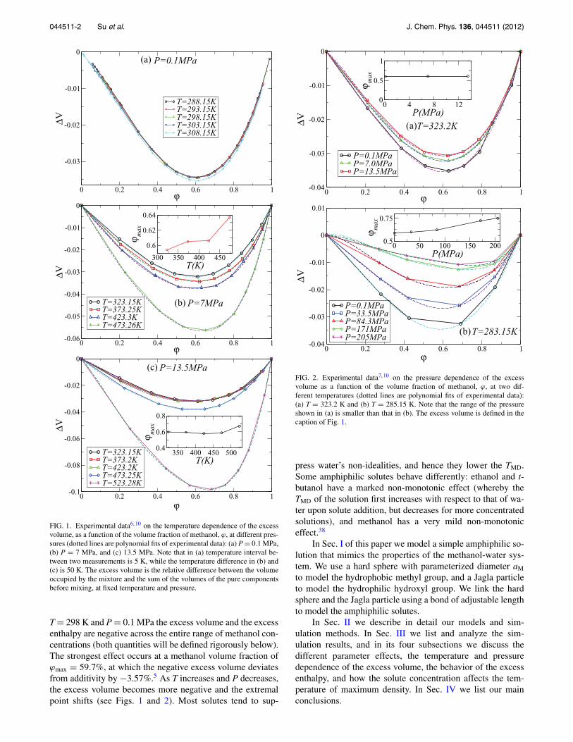
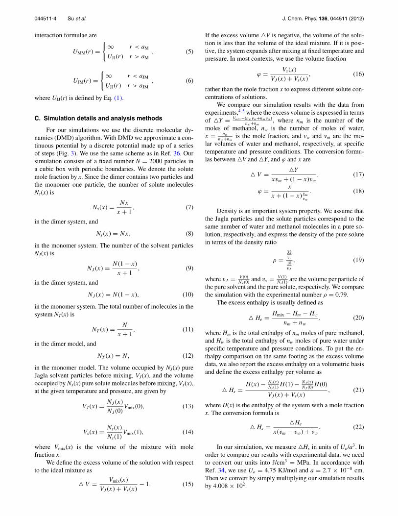
FIG. 1. Experimental data6, 10 on the temperature dependence of the excessvolume, as a function of the volume fraction of methanol, ϕ, at different pres-sures (dotted lines are polynomial fits of experimental data): (a) P = 0.1 MPa,(b) P = 7 MPa, and (c) 13.5 MPa. Note that in (a) temperature interval be-tween two measurements is 5 K, while the temperature difference in (b) and(c) is 50 K. The excess volume is the relative difference between the volumeoccupied by the mixture and the sum of the volumes of the pure componentsbefore mixing, at fixed temperature and pressure.

T = 298 K and P = 0.1 MPa the excess volume and the excessenthalpy are negative across the entire range of methanol con-centrations (both quantities will be defined rigorously below).The strongest effect occurs at a methanol volume fraction ofϕmax = 59.7%, at which the negative excess volume deviatesfrom additivity by −3.57%.5 As T increases and P decreases,the excess volume becomes more negative and the extremalpoint shifts (see Figs. 1 and 2). Most solutes tend to sup-

0 0.2 0.4 0.6 0.8 1ϕ

-0.04

-0.03

-0.02

-0.01

0

ΔV

P=0.1MPaP=7.0MPaP=13.5MPa

0 4 8 12P(MPa)

0

0.5

1

ϕ max

T=323.2K(a)

0 0.2 0.4 0.6 0.8 1ϕ

-0.04

-0.03

-0.02

-0.01

0

0.01

ΔVP=0.1MPaP=33.5MPaP=84.3MPaP=171MPaP=205MPa

0 50 100 150 200P(MPa)

0.5

0.75

ϕ max

T=283.15K(b)

FIG. 2. Experimental data7, 10 on the pressure dependence of the excessvolume as a function of the volume fraction of methanol, ϕ, at two dif-ferent temperatures (dotted lines are polynomial fits of experimental data):(a) T = 323.2 K and (b) T = 285.15 K. Note that the range of the pressureshown in (a) is smaller than that in (b). The excess volume is defined in thecaption of Fig. 1.

press water’s non-idealities, and hence they lower the TMD.Some amphiphilic solutes behave differently: ethanol and t-butanol have a marked non-monotonic effect (whereby theTMD of the solution first increases with respect to that of wa-ter upon solute addition, but decreases for more concentratedsolutions), and methanol has a very mild non-monotoniceffect.38

In Sec. I of this paper we model a simple amphiphilic so-lution that mimics the properties of the methanol-water sys-tem. We use a hard sphere with parameterized diameter aM

to model the hydrophobic methyl group, and a Jagla particleto model the hydrophilic hydroxyl group. We link the hardsphere and the Jagla particle using a bond of adjustable lengthto model the amphiphilic solutes.

In Sec. II we describe in detail our models and sim-ulation methods. In Sec. III we list and analyze the sim-ulation results, and in its four subsections we discuss thedifferent parameter effects, the temperature and pressuredependence of the excess volume, the behavior of the excessenthalpy, and how the solute concentration affects the tem-perature of maximum density. In Sec. IV we list our mainconclusions.

044511-3 Simple amphiphilic solutes in a Jagla solvent J. Chem. Phys. 136, 044511 (2012)

II. MODEL AND METHODS

A. Dimer model for amphiphilic solutes

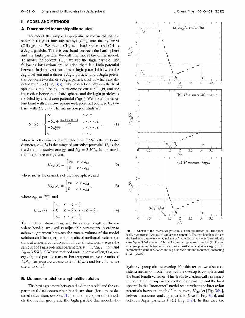
To model the simple amphiphilic solute methanol, weseparate CH3OH into the methyl (CH3) and the hydroxyl(OH) groups. We model CH3 as a hard sphere and OH asa Jagla particle. There is one bond between the hard sphereand the Jagla particle. We call this model the dimer model.To model the solvent, H2O, we use the Jagla particle. Thefollowing interactions are included: there is a Jagla potentialbetween Jagla solvent particles, a Jagla potential between theJagla solvent and a dimer’s Jagla particle, and a Jagla poten-tial between two dimer’s Jagla particles, all of which are de-noted by UJJ(r) [Fig. 3(a)]. The interaction between the hardspheres is modeled by a hard-core potential UHH(r), and theinteraction between the hard spheres and the Jagla particles ismodeled by a hard-core potential UJH(r). We model the cova-lent bond with a narrow square well potential bounded by twohard walls Ubond(r). The interaction potentials are

UJJ(r) =

⎧⎪⎪⎪⎨⎪⎪⎪⎩

∞ r < a

−Uo + (Uo+UR )(b−r)b−a

a < r < b

−Uoc−rc−b

b < r < c

0 r > c

, (1)

where a is the hard core diameter, b = 1.72a is the soft corediameter, c = 3a is the range of attractive potential, Uo is themaximum attractive energy, and UR = 3.56Uo is the maxi-mum repulsive energy, and

UHH (r) ={

∞ r < aM

0 r > aM, (2)

where aM is the diameter of the hard sphere, and

UJH (r) ={

∞ r < aJM

0 r > aJM, (3)

where aJM = aM+a2 and

Ubond(r) =

⎧⎪⎨⎪⎩

∞ r < ζ − δ2

0 ζ − δ2 < r < ζ + δ

2

∞ r > ζ + δ2

. (4)

The hard core diameter aM and the average length of the co-valent bond ζ are used as adjustable parameters in order toachieve agreement between the excess volume of the modelsolution and the experimental results of methanol-water solu-tions at ambient conditions. In all our simulations, we use thesame set of Jagla potential parameters, b = 1.72a, c = 3a, andUR = 3.56Uo.36 We use reduced units in terms of length a, en-ergy Uo, and particle mass m. For temperature we use units ofUo/kB; for pressure we use units of Uo/a3; and for volume weuse units of a3.

B. Monomer model for amphiphilic solutes

The best agreement between the dimer model and the ex-perimental data occurs when bonds are short (for a more de-tailed discussion, see Sec. II), i.e., the hard sphere that mod-els the methyl group and the Jagla particle that models the

0 0.5 1 1.5 2 2.5 3 3.5 4r/a

-1

0

1

2

3

4

UJJ

(r)

(a) Jagla Potential

a b cU

o

UR

0 0.5 1 1.5 2 2.5 3 3.5 4r/a

-1

0

1

2

3

4

UM

M(r

)

(b) Monomer-Monomer

aM b c

0 0.5 1 1.5 2 2.5 3 3.5 4r/a

-1

0

1

2

3

4

UJM

(r)

(c) Monomer-Jagla

(aM

+a)/2b c

FIG. 3. Sketch of the interaction potentials in our simulation. (a) The spher-ically symmetric “two-scale” Jagla ramp potential. The two length scales arethe hard core diameter r = a, and the soft core diameter r = b. We study thecase UR = 3.56U0, b = 1.72a, and a long range cutoff c = 3a. (b) The in-teraction potential between two monomers, with contact distance aM. (c) Theinteraction potential between the Jagla particle and the monomer, contactingat (a + aM)/2.

hydroxyl group almost overlap. For this reason we also con-sider a methanol model in which the overlap is complete, andthe bond length vanishes. This leads to a spherically symmet-ric potential that superimposes the Jagla particle and the hardsphere. In this “monomer” model we introduce the interactionpotentials between “methyl” monomers, UMM(r) [Fig. 3(b)],between monomer and Jagla particle, UJM(r) [Fig. 3(c)], andbetween Jagla particles UJJ(r) [Fig. 3(a)]. In this case the

044511-4 Su et al. J. Chem. Phys. 136, 044511 (2012)

interaction formulae are

UMM(r) ={

∞ r < aM

UJJ(r) r > aM, (5)

UJM(r) ={

∞ r < aJM

UJJ(r) r > aJM, (6)

where UJJ(r) is defined by Eq. (1).

C. Simulation details and analysis methods

For our simulations we use the discrete molecular dy-namics (DMD) algorithm. With DMD we approximate a con-tinuous potential by a discrete potential made up of a seriesof steps (Fig. 3). We use the same scheme as in Ref. 36. Oursimulation consists of a fixed number N = 2000 particles ina cubic box with periodic boundaries. We denote the solutemole fraction by x. Since the dimer contains two particles andthe monomer one particle, the number of solute moleculesNs(x) is

Ns(x) = Nx

x + 1, (7)

in the dimer system, and

Ns(x) = Nx, (8)

in the monomer system. The number of the solvent particlesNJ(x) is

NJ (x) = N (1 − x)

x + 1, (9)

in the dimer system, and

NJ (x) = N (1 − x), (10)

in the monomer system. The total number of molecules in thesystem NT(x) is

NT (x) = N

x + 1, (11)

in the dimer model, and

NT (x) = N, (12)

in the monomer model. The volume occupied by NJ(x) pureJagla solvent particles before mixing, VJ(x), and the volumeoccupied by Ns(x) pure solute molecules before mixing, Vs(x),at the given temperature and pressure, are given by

VJ (x) = NJ (x)

NJ (0)Vmix(0), (13)

Vs(x) = Ns(x)

Ns(1)Vmix(1), (14)

where Vmix(x) is the volume of the mixture with molefraction x.

We define the excess volume of the solution with respectto the ideal mixture as

� V = Vmix(x)

VJ (x) + Vs(x)− 1. (15)

If the excess volume �V is negative, the volume of the solu-tion is less than the volume of the ideal mixture. If it is posi-tive, the system expands after mixing at fixed temperature andpressure. In most contexts, we use the volume fraction

ϕ = Vs(x)

VJ (x) + Vs(x), (16)

rather than the mole fraction x to express different solute con-centrations of solutions.

We compare our simulation results with the data fromexperiments,4, 5 where the excess volume is expressed in termsof �Y = Vmix−(nwvw+nmvm)

nw+nm, where nm is the number of the

moles of methanol, nw is the number of moles of water,x = nm

nw+nmis the mole fraction, and vw and vm are the mo-

lar volumes of water and methanol, respectively, at specifictemperature and pressure conditions. The conversion formu-las between �V and �Y, and ϕ and x are

� V = �Y

xvm + (1 − x)vw

, (17)

ϕ = x

x + (1 − x) vw

vm

. (18)

Density is an important system property. We assume thatthe Jagla particles and the solute particles correspond to thesame number of water and methanol molecules in a pure so-lution, respectively, and express the density of the pure solutein terms of the density ratio

ρ =32vs

18vJ

, (19)

where vJ = V (0)NJ (0) and vs = V (1)

Ns (1) are the volume per particle ofthe pure solvent and the pure solute, respectively. We comparethe simulation with the experimental number ρ = 0.79.

The excess enthalpy is usually defined as

� He = Hmix − Hm − Hw

nm + nw

, (20)

where Hm is the total enthalpy of nm moles of pure methanol,and Hw is the total enthalpy of nw moles of pure water underspecific temperature and pressure conditions. To put the en-thalpy comparison on the same footing as the excess volumedata, we also report the excess enthalpy on a volumetric basisand define the excess enthalpy per volume as

� Hs =H (x) − Ns (x)

Ns (1) H (1) − NJ (x)NJ (0) H (0)

VJ (x) + Vs(x), (21)

where H(x) is the enthalpy of the system with a mole fractionx. The conversion formula is

� Hs = �He

x(vm − vw) + vw

. (22)

In our simulation, we measure �Hs in units of Uo/a3. Inorder to compare our results with experimental data, we needto convert our units into J/cm3 = MPa. In accordance withRef. 34, we use Uo = 4.75 KJ/mol and a = 2.7 × 10−8 cm.Then we convert by simply multiplying our simulation resultsby 4.008 × 102.

044511-5 Simple amphiphilic solutes in a Jagla solvent J. Chem. Phys. 136, 044511 (2012)

III. RESULTS AND DISCUSSION

A. Effects of the parameters on model behavior

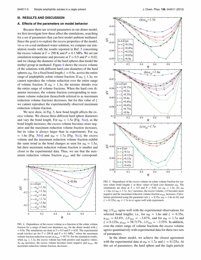
Because there are several parameters in our dimer model,we first investigate how these affect the simulations, searchingfor a set of parameters that can best model ambient methanol.Since the goal is to explore the excess properties of the model,vis-a-vis a real methanol-water solution, we compare our sim-ulation results with the results reported in Ref. 5 concerningthe excess volume at T = 298 K and P = 0.1 MPa. We set oursimulation temperature and pressure at T = 0.5 and P = 0.02,and we change the diameter of the hard spheres that model themethyl group in methanol. Figure 4 shows the excess volumeof the solutions with different hard core diameters of the hardspheres aM, for a fixed bond length ζ = 0.9a, across the entirerange of amphiphilic solute volume fraction. If aM ≤ 1.3a, wecannot reproduce the volume reduction over the entire rangeof volume fraction. If aM > 1.3a, the mixture shrinks overthe entire range of volume fractions. When the hard core di-ameter increases, the volume fraction corresponding to max-imum volume reduction (henceforth referred to as maximumreduction volume fraction) decreases, but for this value of ζ

we cannot reproduce the experimentally observed maximumreduction volume fraction.

We next show, in Fig. 5, how bond length affects the ex-cess volume. We choose three different hard sphere diametersand vary the bond length. For aM = 1.5a [Fig. 5(a)], as thebond length increases, the excess volume becomes more neg-ative and the maximum reduction volume fraction increases,but its value is always larger than in experiments. For aM

= 1.6a [Fig. 5(b)] and aM = 1.7a [Fig. 5(c)], the excessvolume and the maximum reduction volume fraction exhibitthe same trend as the bond changes as seen for aM = 1.5a,but their maximum reduction volume fraction is smaller andcloser to the experimental data. Thus, we see that the max-imum reduction volume fraction ϕmax and the correspond-

0 0.2 0.4 0.6 0.8 1ϕ

-0.3

-0.2

-0.1

0

ΔV

Expt.a

M=1.3a

aM

=1.5aa

M=1.6a

aM

=1.7aa

M=1.8a

aM

=2.0a

ζ=0.9a

FIG. 4. Dependence of the excess volume as a function of the solute volumefraction for a range of hard core diameters aM, for the dimer model with ζ

= 0.9a. The simulations are done at T = 0.5 and P = 0.02. The experimentalresult (circles) are for T = 298 K and P = 0.1 MPa,5 where the maximumvolume fraction reduction occurs at ϕmax ≈ 59.7%. For the simulation results,when aM ≤ 1.3a, the excess volume has both positive and negative values.As aM increases, the excess volume becomes more negative and ϕmax, themaximum reduction volume fraction, decreases.

0 0.2 0.4 0.6 0.8 1ϕ

-0.05

-0.04

-0.03

-0.02

-0.01

0

ΔV Expt.ζ=0.35aζ=0.45aζ=0.55aζ=0.65aζ=0.9a

(a)aM

=1.5a

A

A

A

A

A

A

A

A A

A

A

0 0.2 0.4 0.6 0.8 1ϕ

-0.1

-0.08

-0.06

-0.04

-0.02

0

ΔV

Expt.ζ=0.15aζ=0.2aζ=0.35aζ=0.4aζ=0.45aζ=0.65aζ=0.75aζ=0.9aA A

(b)aM

=1.6a

0 0.2 0.4 0.6 0.8 1ϕ

-0.08

-0.06

-0.04

-0.02

0

ΔV Expt.ζ=0.1aζ=0.125aζ=0.15aζ=0.35aζ=0.45a

(c) aM

=1.7a

FIG. 5. Dependence of the excess volume on solute volume fraction for var-ious solute bond lengths ζ at three values of hard core diameter aM. Thesimulations are done at T = 0.5 and P = 0.02. (a) aM = 1.5a, (b) aM= 1.6a, (c) aM = 1.7a. As ζ increases, the excess volume, �V becomes morenegative and the maximum reduction volume fraction ϕmax increases. Calcu-lations performed using the parameter sets ζ = 0.35a, aM = 1.6a in (b), andζ = 0.125a, aM = 1.7a in (c) agree well with experiment.

ing �Vmax agree well with the experimental observations forselected bond lengths; i.e., for aM = 1.6a and ζ = 0.35a,ϕmax = 63.6%, �Vmax = −3.67%, and for aM = 1.7a andζ = 0.125a, ϕmax = 58.717%, �Vmax = −3.55%. In addition,over the entire range of volume fractions the excess volumeagrees quantitatively with experimental data for these two setsof parameters.

In the dimer model, we achieve the closest agreementwith the experimental data at aM = 1.7a and ζ = 0.125a. Atthis set of parameters, the hard sphere and the Jagla particle

044511-6 Su et al. J. Chem. Phys. 136, 044511 (2012)

AA

AA

A A AA

A

A

A

0 0.2 0.4 0.6 0.8 1ϕ

-0.08

-0.06

-0.04

-0.02

0ΔV

Expt.a

M=1.68aA A

aM

=1.72a

aM

=1.73a

aM

=1.74a

aM

=1.75a

aM

=1.76a

aM

=1.8a

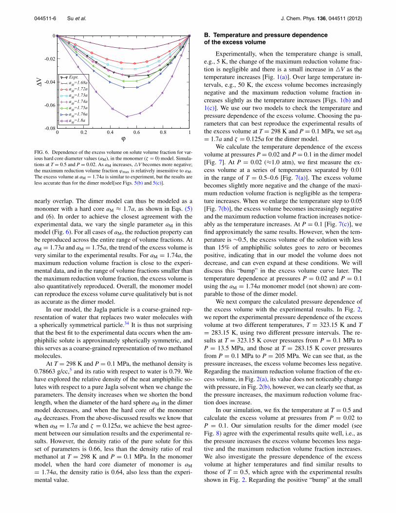
FIG. 6. Dependence of the excess volume on solute volume fraction for var-ious hard core diameter values (aM), in the monomer (ζ = 0) model. Simula-tions at T = 0.5 and P = 0.02. As aM increases, �V becomes more negative;the maximum reduction volume fraction ϕmax is relatively insensitive to aM.The excess volume at aM = 1.74a is similar to experiment, but the results areless accurate than for the dimer model[see Figs. 5(b) and 5(c)].

nearly overlap. The dimer model can thus be modeled as amonomer with a hard core aM ≈ 1.7a, as shown in Eqs. (5)and (6). In order to achieve the closest agreement with theexperimental data, we vary the single parameter aM in thismodel (Fig. 6). For all cases of aM, the reduction property canbe reproduced across the entire range of volume fractions. AtaM = 1.73a and aM = 1.75a, the trend of the excess volume isvery similar to the experimental results. For aM = 1.74a, themaximum reduction volume fraction is close to the experi-mental data, and in the range of volume fractions smaller thanthe maximum reduction volume fraction, the excess volume isalso quantitatively reproduced. Overall, the monomer modelcan reproduce the excess volume curve qualitatively but is notas accurate as the dimer model.

In our model, the Jagla particle is a coarse-grained rep-resentation of water that replaces two water molecules witha spherically symmetrical particle.34 It is thus not surprisingthat the best fit to the experimental data occurs when the am-phiphilic solute is approximately spherically symmetric, andthis serves as a coarse-grained representation of two methanolmolecules.

At T = 298 K and P = 0.1 MPa, the methanol density is0.78663 g/cc,5 and its ratio with respect to water is 0.79. Wehave explored the relative density of the neat amphiphilic so-lutes with respect to a pure Jagla solvent when we change theparameters. The density increases when we shorten the bondlength, when the diameter of the hard sphere aM in the dimermodel decreases, and when the hard core of the monomeraM decreases. From the above-discussed results we know thatwhen aM = 1.7a and ζ = 0.125a, we achieve the best agree-ment between our simulation results and the experimental re-sults. However, the density ratio of the pure solute for thisset of parameters is 0.66, less than the density ratio of realmethanol at T = 298 K and P = 0.1 MPa. In the monomermodel, when the hard core diameter of monomer is aM

= 1.74a, the density ratio is 0.64, also less than the experi-mental value.

B. Temperature and pressure dependenceof the excess volume

Experimentally, when the temperature change is small,e.g., 5 K, the change of the maximum reduction volume frac-tion is negligible and there is a small increase in �V as thetemperature increases [Fig. 1(a)]. Over large temperature in-tervals, e.g., 50 K, the excess volume becomes increasinglynegative and the maximum reduction volume fraction in-creases slightly as the temperature increases [Figs. 1(b) and1(c)]. We use our two models to check the temperature andpressure dependence of the excess volume. Choosing the pa-rameters that can best reproduce the experimental results ofthe excess volume at T = 298 K and P = 0.1 MPa, we set aM

= 1.7a and ζ = 0.125a for the dimer model.We calculate the temperature dependence of the excess

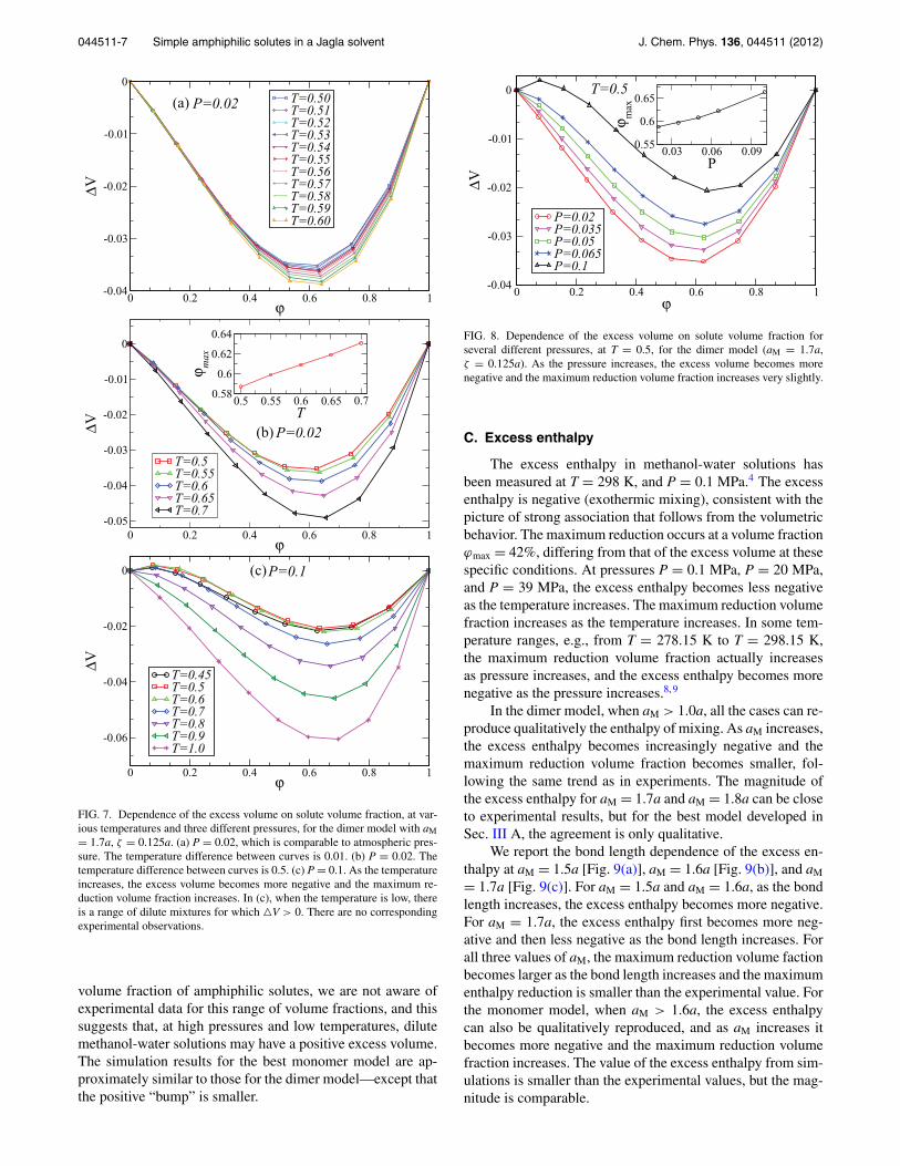
volume at pressures P = 0.02 and P = 0.1 in the dimer model[Fig. 7]. At P = 0.02 (≈1.0 atm), we first measure the ex-cess volume at a series of temperatures separated by 0.01in the range of T = 0.5–0.6 [Fig. 7(a)]. The excess volumebecomes slightly more negative and the change of the maxi-mum reduction volume fraction is negligible as the tempera-ture increases. When we enlarge the temperature step to 0.05[Fig. 7(b)], the excess volume becomes increasingly negativeand the maximum reduction volume fraction increases notice-ably as the temperature increases. At P = 0.1 [Fig. 7(c)], wefind approximately the same results. However, when the tem-perature is ∼0.5, the excess volume of the solution with lessthan 15% of amphiphilic solutes goes to zero or becomespositive, indicating that in our model the volume does notdecrease, and can even expand at these conditions. We willdiscuss this “bump” in the excess volume curve later. Thetemperature dependence at pressures P = 0.02 and P = 0.1using the aM = 1.74a monomer model (not shown) are com-parable to those of the dimer model.

We next compare the calculated pressure dependence ofthe excess volume with the experimental results. In Fig. 2,we report the experimental pressure dependence of the excessvolume at two different temperatures, T = 323.15 K and T= 283.15 K, using two different pressure intervals. The re-sults at T = 323.15 K cover pressures from P = 0.1 MPa toP = 13.5 MPa, and those at T = 283.15 K cover pressuresfrom P = 0.1 MPa to P = 205 MPa. We can see that, as thepressure increases, the excess volume becomes less negative.Regarding the maximum reduction volume fraction of the ex-cess volume, in Fig. 2(a), its value does not noticeably changewith pressure, in Fig. 2(b), however, we can clearly see that, asthe pressure increases, the maximum reduction volume frac-tion does increase.

In our simulation, we fix the temperature at T = 0.5 andcalculate the excess volume at pressures from P = 0.02 toP = 0.1. Our simulation results for the dimer model (seeFig. 8) agree with the experimental results quite well, i.e., asthe pressure increases the excess volume becomes less nega-tive and the maximum reduction volume fraction increases.We also investigate the pressure dependence of the excessvolume at higher temperatures and find similar results tothose of T = 0.5, which agree with the experimental resultsshown in Fig. 2. Regarding the positive “bump” at the small

044511-7 Simple amphiphilic solutes in a Jagla solvent J. Chem. Phys. 136, 044511 (2012)

A

A

A

A

A

A

AA

A

A

A

0 0.2 0.4 0.6 0.8 1ϕ

-0.04

-0.03

-0.02

-0.01

0ΔV

T=0.50T=0.51T=0.52T=0.53T=0.54T=0.55T=0.56T=0.57T=0.58A A

T=0.59T=0.60

(a) P=0.02

0 0.2 0.4 0.6 0.8 1ϕ

-0.05

-0.04

-0.03

-0.02

-0.01

0

ΔV

T=0.5T=0.55T=0.6T=0.65T=0.7

0.5 0.55 0.6 0.65 0.7T

0.58

0.6

0.62

0.64

ϕ max

(b) P=0.02

0 0.2 0.4 0.6 0.8 1ϕ

-0.06

-0.04

-0.02

0

ΔV

T=0.45T=0.5T=0.6T=0.7T=0.8T=0.9T=1.0

(c)P=0.1

FIG. 7. Dependence of the excess volume on solute volume fraction, at var-ious temperatures and three different pressures, for the dimer model with aM= 1.7a, ζ = 0.125a. (a) P = 0.02, which is comparable to atmospheric pres-sure. The temperature difference between curves is 0.01. (b) P = 0.02. Thetemperature difference between curves is 0.5. (c) P = 0.1. As the temperatureincreases, the excess volume becomes more negative and the maximum re-duction volume fraction increases. In (c), when the temperature is low, thereis a range of dilute mixtures for which �V > 0. There are no correspondingexperimental observations.

volume fraction of amphiphilic solutes, we are not aware ofexperimental data for this range of volume fractions, and thissuggests that, at high pressures and low temperatures, dilutemethanol-water solutions may have a positive excess volume.The simulation results for the best monomer model are ap-proximately similar to those for the dimer model—except thatthe positive “bump” is smaller.

0 0.2 0.4 0.6 0.8 1ϕ

-0.04

-0.03

-0.02

-0.01

0

ΔV

P=0.02P=0.035P=0.05P=0.065P=0.1

0.03 0.06 0.09P

0.55

0.6

0.65

ϕ max

T=0.5

FIG. 8. Dependence of the excess volume on solute volume fraction forseveral different pressures, at T = 0.5, for the dimer model (aM = 1.7a,ζ = 0.125a). As the pressure increases, the excess volume becomes morenegative and the maximum reduction volume fraction increases very slightly.

C. Excess enthalpy

The excess enthalpy in methanol-water solutions hasbeen measured at T = 298 K, and P = 0.1 MPa.4 The excessenthalpy is negative (exothermic mixing), consistent with thepicture of strong association that follows from the volumetricbehavior. The maximum reduction occurs at a volume fractionϕmax = 42%, differing from that of the excess volume at thesespecific conditions. At pressures P = 0.1 MPa, P = 20 MPa,and P = 39 MPa, the excess enthalpy becomes less negativeas the temperature increases. The maximum reduction volumefraction increases as the temperature increases. In some tem-perature ranges, e.g., from T = 278.15 K to T = 298.15 K,the maximum reduction volume fraction actually increasesas pressure increases, and the excess enthalpy becomes morenegative as the pressure increases.8, 9

In the dimer model, when aM > 1.0a, all the cases can re-produce qualitatively the enthalpy of mixing. As aM increases,the excess enthalpy becomes increasingly negative and themaximum reduction volume fraction becomes smaller, fol-lowing the same trend as in experiments. The magnitude ofthe excess enthalpy for aM = 1.7a and aM = 1.8a can be closeto experimental results, but for the best model developed inSec. III A, the agreement is only qualitative.

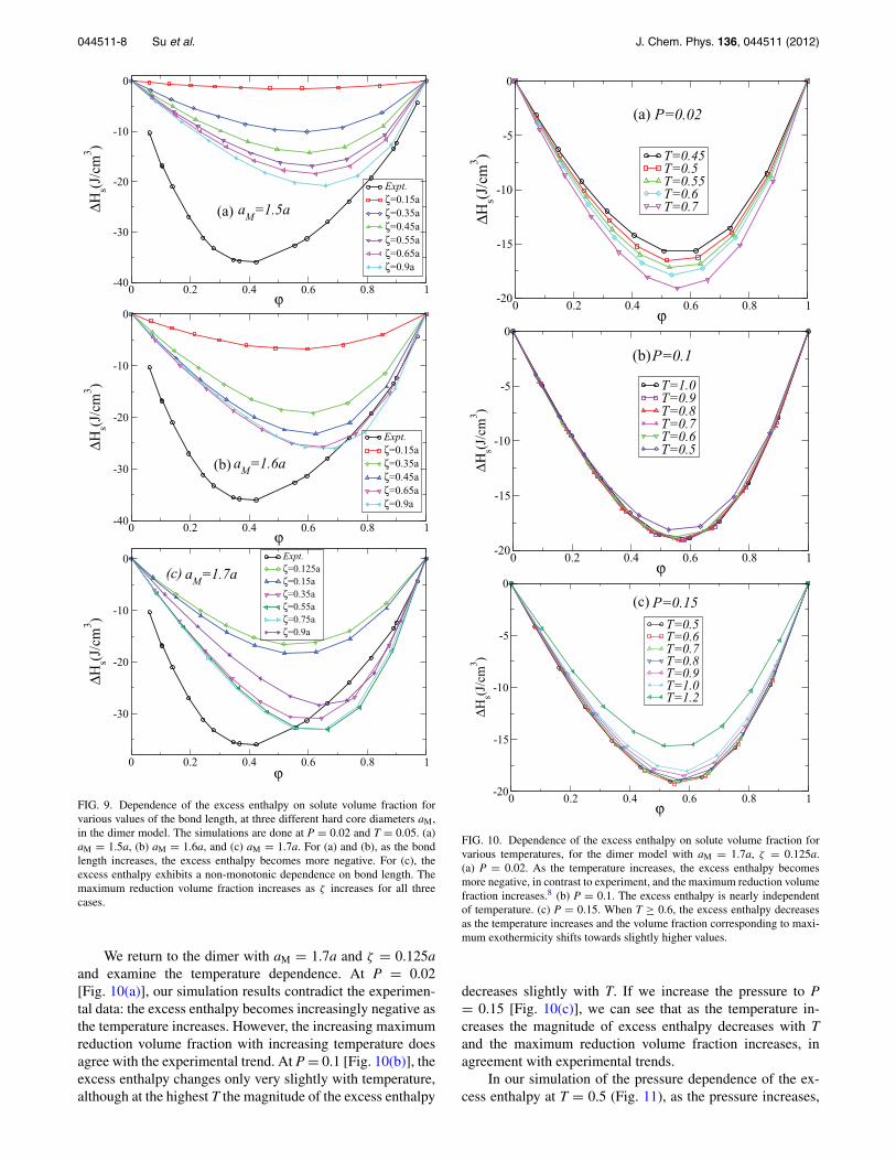
We report the bond length dependence of the excess en-thalpy at aM = 1.5a [Fig. 9(a)], aM = 1.6a [Fig. 9(b)], and aM

= 1.7a [Fig. 9(c)]. For aM = 1.5a and aM = 1.6a, as the bondlength increases, the excess enthalpy becomes more negative.For aM = 1.7a, the excess enthalpy first becomes more neg-ative and then less negative as the bond length increases. Forall three values of aM, the maximum reduction volume factionbecomes larger as the bond length increases and the maximumenthalpy reduction is smaller than the experimental value. Forthe monomer model, when aM > 1.6a, the excess enthalpycan also be qualitatively reproduced, and as aM increases itbecomes more negative and the maximum reduction volumefraction increases. The value of the excess enthalpy from sim-ulations is smaller than the experimental values, but the mag-nitude is comparable.

044511-8 Su et al. J. Chem. Phys. 136, 044511 (2012)

0 0.2 0.4 0.6 0.8 1ϕ

-40

-30

-20

-10

0ΔH

s(J/c

m3 )

Expt.ζ=0.15aζ=0.35aζ=0.45aζ=0.55aζ=0.65aζ=0.9a

aM

=1.5a(a)

0 0.2 0.4 0.6 0.8 1ϕ

-40

-30

-20

-10

0

ΔHs(J

/cm

3 )

Expt.ζ=0.15aζ=0.35aζ=0.45aζ=0.65aζ=0.9a

aM

=1.6a(b)

0 0.2 0.4 0.6 0.8 1ϕ

-30

-20

-10

0

ΔHs(J

/cm

3 )

Expt.ζ=0.125aζ=0.15aζ=0.35aζ=0.55aζ=0.75aζ=0.9a

aM

=1.7a(c)

FIG. 9. Dependence of the excess enthalpy on solute volume fraction forvarious values of the bond length, at three different hard core diameters aM,in the dimer model. The simulations are done at P = 0.02 and T = 0.05. (a)aM = 1.5a, (b) aM = 1.6a, and (c) aM = 1.7a. For (a) and (b), as the bondlength increases, the excess enthalpy becomes more negative. For (c), theexcess enthalpy exhibits a non-monotonic dependence on bond length. Themaximum reduction volume fraction increases as ζ increases for all threecases.

We return to the dimer with aM = 1.7a and ζ = 0.125aand examine the temperature dependence. At P = 0.02[Fig. 10(a)], our simulation results contradict the experimen-tal data: the excess enthalpy becomes increasingly negative asthe temperature increases. However, the increasing maximumreduction volume fraction with increasing temperature doesagree with the experimental trend. At P = 0.1 [Fig. 10(b)], theexcess enthalpy changes only very slightly with temperature,although at the highest T the magnitude of the excess enthalpy

0 0.2 0.4 0.6 0.8 1ϕ

-20

-15

-10

-5

0

ΔHs(J

/cm

3 ) T=0.45T=0.5T=0.55T=0.6T=0.7

(a) P=0.02

0 0.2 0.4 0.6 0.8 1ϕ

-20

-15

-10

-5

0

ΔΗs(J

/cm

3 )

T=1.0T=0.9T=0.8T=0.7T=0.6T=0.5

(b)P=0.1

0 0.2 0.4 0.6 0.8 1ϕ

-20

-15

-10

-5

0

ΔHs(J

/cm

3 )

T=0.5T=0.6T=0.7T=0.8T=0.9T=1.0T=1.2

(c) P=0.15

FIG. 10. Dependence of the excess enthalpy on solute volume fraction forvarious temperatures, for the dimer model with aM = 1.7a, ζ = 0.125a.(a) P = 0.02. As the temperature increases, the excess enthalpy becomesmore negative, in contrast to experiment, and the maximum reduction volumefraction increases.8 (b) P = 0.1. The excess enthalpy is nearly independentof temperature. (c) P = 0.15. When T ≥ 0.6, the excess enthalpy decreasesas the temperature increases and the volume fraction corresponding to maxi-mum exothermicity shifts towards slightly higher values.

decreases slightly with T. If we increase the pressure to P= 0.15 [Fig. 10(c)], we can see that as the temperature in-creases the magnitude of excess enthalpy decreases with Tand the maximum reduction volume fraction increases, inagreement with experimental trends.

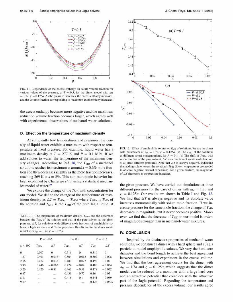
In our simulation of the pressure dependence of the ex-cess enthalpy at T = 0.5 (Fig. 11), as the pressure increases,

044511-9 Simple amphiphilic solutes in a Jagla solvent J. Chem. Phys. 136, 044511 (2012)

0 0.2 0.4 0.6 0.8 1ϕ

-20

-15

-10

-5

0

ΔHs(J

/cm

3 )

P=0.02P=0.035P=0.065P=0.1P=0.15

T=0.5

FIG. 11. Dependence of the excess enthalpy on solute volume fraction forvarious values of the pressure, at T = 0.5, for the dimer model with aM= 1.7a, ζ = 0.125a. As the pressure increases, the excess enthalpy increases,and the volume fraction corresponding to maximum exothermicity increases.

the excess enthalpy becomes more negative and the maximumreduction volume fraction becomes larger, which agrees wellwith experimental observations of methanol-water solutions.

D. Effect on the temperature of maximum density

At sufficiently low temperatures and pressures, the den-sity of liquid water exhibits a maximum with respect to tem-perature at fixed pressure. For example, liquid water has amaximum density at T = 277 K and P = 0.1 MPa. If weadd solutes to water, the temperature of the maximum den-sity changes. According to Ref. 38, the TMD of a methanolsolutions reaches its maximum at around x = 0.6% mole frac-tion and then decreases slightly as the mole fraction increases,reaching 269 K at x = 5%. This non-monotonic behavior hasbeen explained by Chatterjee et al. using a statistical mechan-ics model of water.39

We explore the change of the TMD with concentration forour model. We define the change of the temperature of max-imum density as �T = TMDs − TMDJ where TMDs is TMD ofthe solution and TMDJ is the TMD of the pure Jagla liquid, at

TABLE I. The temperature of maximum density, TMD, and the differencebetween the TMD of the solution and that of the pure solvent at the givenpressure, �T, for solutions with different mole fractions of amphiphilic so-lutes in Jagla solvents, at different pressures. Results are for the dimer solutemodel with aM = 1.7a, ζ = 0.125a.

P = 0.065 P = 0.1 P = 0.15

x × 100 TMD �T TMD �T TMD �T

0 0.507 0 0.516 0 0.510 01.27 0.491 − 0.016 0.504 − 0.012 0.502 − 0.0082.56 0.472 − 0.035 0.489 − 0.027 0.490 − 0.023.90 0.446 − 0.062 0.474 − 0.04 0.486 − 0.0245.26 0.426 − 0.81 0.462 − 0.51 0.478 − 0.0326.67 . . . . . . 0.439 − 0.77 0.46 − 0.058.11 . . . . . . 0.416 − 0.1 0.441 − 0.0699.59 . . . . . . . . . . . . 0.426 − 0.0837

0 0.02 0.04 0.06 0.08x

0.4

0.42

0.44

0.46

0.48

0.5

0.52

TM

D

P=0.1(a)

0 0.02 0.04 0.06 0.08 0.1x

-0.1

-0.08

-0.06

-0.04

-0.02

0

ΔΤ

P=0.065P=0.1P=0.15

(b)

FIG. 12. Effect of amphiphilic solutes on TMD of solutions. We use the dimerwith parameters of aM = 1.7a, ζ = 0.125a. (a) The TMD of the solutionsat different solute concentrations, for P = 0.1. (b) The shift of TMD, withrespect to that of the pure solvent, �T, as a function of solute mole fraction,x, at three different pressures. Note that �T is always negative, indicatingthat adding solute lowers the solution’s TMD (lower temperatures are neededto observe negative thermal expansion). For a given mixture, the magnitudeof �T decreases as the pressure increases.

the given pressure. We have carried out simulations at threedifferent pressures for the case of dimer with aM = 1.7a andζ = 0.125a. Our results are shown in Table I and Fig. 12.We find that �T is always negative and its absolute valueincreases monotonically with solute mole fraction. If we in-crease pressure for the same mole fraction, the change of TMD

decreases in magnitude, but it never becomes positive. More-over, we find that the decrease of TMD in our model is ordersof magnitude stronger than in methanol-water mixtures.

IV. CONCLUSION

Inspired by the distinctive properties of methanol-watersolutions, we construct a dimer with a hard sphere and a Jaglaparticle to model amphiphilic solutes. We vary the hard corediameter and the bond length to achieve the best agreementbetween simulations and experiment in the excess volume.We find that the best agreement occurs for the dimer withaM = 1.7a and ζ = 0.125a, which suggests that the dimermodel can be reduced to a monomer with a large hard coreand an attractive potential that coincides with the attractivepart of the Jagla potential. Regarding the temperature andpressure dependence of the excess volume, our results agree

044511-10 Su et al. J. Chem. Phys. 136, 044511 (2012)

qualitatively with experimental data. Our model reproducesthe excess enthalpy of the methanol solutions less accuratelythan the excess volume. This is related to the fact that, in oursimple model of amphiphilic solutes, we use the unchangedJagla potential for the amphiphilic group. We speculate that abetter agreement could be achieved if we varied the potentialof the amphiphilic group. When we investigate the effect ofthe amphiphilic solute on the temperature of maximum den-sity of a solution, we find that unlike in water-methanol so-lution, the TMD monotonically decreases with solute concen-trations. Moreover, the effect of concentration in the model isorders of magnitude stronger than in experiments.

ACKNOWLEDGMENTS

Z.S. and H.E.S. thank the National Science Foundation(NSF) Chemistry Division (Grant No. CHE 0908218) for sup-port. S.V.B. acknowledges the partial support of this researchby the Dr. Bernard W. Gamson Computational Science Centerat Yeshiva College. P.G.D. and P.J.R. gratefully acknowledgethe support of the NSF (Collaborative Research Grant Nos.CHE-0908265 and CHE-0910615). P.J.R. also gratefully ac-knowledges additional support from the R. A. Welch Founda-tion (F-0019).

1G. Akerlof, J. Am. Chem. Soc. 54, 4126 (1932).2R. E. Gibson, J. Am. Chem. Soc. 57, 1551 (1935).3H. Frank and M. Evans, J. Chem. Phys. 13, 507 (1945)4R. F. Lama and C.-Y. Lu, J. Chem. Eng. Data 10, 216 (1965).5M. L. McGlashan and A. G. Williamson, J. Chem. Eng. Data 21, 196(1976).

6G. C. Benson, and O. Kiyohara, J. Sol. Chem. 9, 791 (1980).7H. Kubota, Y. Tanaka, and T. Makita, Int. J. Thermophys. 9, 47 (1987).8I. Tomaszkiewicz, S. L. Randzio, and P. Gireycz, Thermochim. Acta 103,281 (1986).

9I. Tomaszkiewicz and S. L. Randzio, Thermochim. Acta 103, 291(1986).

10C. B. Xiao, and H. Bianchi, and P. R. Tremaine, J. Chem. Thermdyn. 29,261 (1997).

11T. Sato, A. Chiba, and R. Nozaki, J. Chem. Phys. 112, 2924 (2000).

12B. Hribar-Lee and K. A. Dill, Acta Chim. Slov. 53, 257 (2006), http://acta.chem-soc.si/53/graph/acta-53(3)-GA.htm.

13W. L. Jorgensen, J. Phys. Chem. 90, 1276 (1986).14H. J.C. Berendsen, J. R. Grigera, and T. P. Straattsma, J. Phys. Chem. 91,

6269 (1987).15W. L. Jorgensen, J. Chandrasekhar, J. D. Madura, R. W. Impey, and

M. L. Klein, J. Chem. Phys. 79, 926 (1983).16W. L. Jorgensen and J. D. Madura, Mol. Phys. 56, 1381 (1985).17M. W. Mahoney and W. L. Jorgensen, J. Chem. Phys. 112, 8910 (2000).18K. A. Silverstein, A. D. Haymet, and K. A. Dill, J. Am. Chem. Soc. 120,

3166 (1998).19C. L. Dias, T. Ala-Nissila, M. Grant, and M. Karttunen, J. Chem. Phys. 131,

054505 (2009).20J.-P. Becker and O. Collet, J. Mol. Struct.: THEOCHEM 774, 23 (2006).21C. L. Dias, T. Ala-Nissila, M. Karttunen, I. Vattulainen, and M. Grant, Phys.

Rev. Lett. 100, 118101 (2008).22C. L. Dias, T. Ala-Nissila, J. Wong-ekkabut, I. Vattulainen, M. Grant, and

M. Karttunen, Cryobiology 60, 91 (2010).23C. L. Dias, T. Hynninen, T. Ala-Nissila, A. S. Foster, and M. Karttunen, J.

Chem. Phys. 134, 065106 (2011).24M. Rerrario, M. Haughney, I. R. McDonald, and M. Klein, J. Chem. Phys.

93, 5156 (1990).25H. Tanaka and K. E. Gubbins, J. Chem. Phys. 97, 2626 (1992).26E. J.W. Wensink, A. C. Hoffmann, P. J. van Maaren, and D. van der Spoel,

J. Chem. Phys. 119, 7308 (2003).27D. Gonzalez-Salgado and I. Nezbeda, Fluid Phase Equilib. 240, 161 (2006).28I. Bako, T. Megyes, S. Balint, T. Grosz, and V. Chihaia, Phys. Chem. Chem.

Phys. 10, 5004 (2008).29Y. Zhong, G. L. Warren, and S. Patel, J. Comput. Chem. 29, 1142 (2008).30E. A. Jagla, Phys. Rev. E 63, 061501 (2001).31J. R. Errington, and P. G. Debenedetti, Nature (London) 409, 318 (2001).32Z. Yan, S. V. Buldyrev, N. Giovambattista, and H. E. Stanley, Phys. Rev.

Lett. 95, 130604 (2005).33Z. Yan, S. V. Buldyrev, N. Giovambattista, P. G. Debenedetti, and

H. E. Stanley, Phys. Rev. E 73, 051204 (2006).34Z. Yan, S. V. Buldyrev, P. Kumar, N. Giovambattista, and H. E. Stanley,

Phys. Rev. E 77, 042201 (2008).35L. Xu, P. Kumar, S. V. Buldyrev, S.-H. Chen, P. Poole, F. Sciortino, and

H. E. Stanley, Proc. Natl. Acad. Sci. U.S.A. 102, 16807 (2005).36L. Xu, S. V. Buldyrev, C. A. Angell, and H. E. Stanley, Phys. Rev. E 74,

031108 (2006).37S. V. Buldyrev, P. Kumar, P. G. Debenedetti, P. J. Rossky, and H. E. Stanley,

Proc. Natl. Acad. Sci. U.S.A. 104, 20177 (2007).38G. Wada and S. Umeda, Bull. Chem. Soc. Jpn. 35, 646 (1962).39S. Chatterjee, H. S. Ashbaugh, and P. G. Debenedetti, J. Chem. Phys. 123,

164503 (2005).