Modeling requirements for large-eddy simulation of turbulent flows

Center for Turbulence ResearchProceedings of the Summer Program 2008

195

Modeling requirements for large-eddy simulationof turbulent flows under supercritical

thermodynamic conditions

By L. Selle† AND G. Ribert‡

The thermodynamic and transport properties of fluids above their critical point is farfrom that of a perfect gas. Strong non-linearities in the equation of state and transportproperties may modify the structure of turbulence but also require additional terms inturbulence models. The present work addresses the influence of a real-gas equation ofstate (Peng-Robinson) on turbulence properties and turbulence models. Direct numeri-cal simulations of temporal jet and homogeneous isotropic turbulence are used for the a

priori analysis of turbulence models within the large-eddy simulation framework. Large-eddy simulations of the same configurations are conducted for an a posteriori analysisof model performance. The a priori analysis suggests that LES models perform as wellunder supercritical conditions, as for a perfect gas. Single-species Homogeneous isotropicturbulence cases also show virtually identical features irrespectively of the thermody-namic conditions. Jets however are significantly affected by the strong density gradientsand the a posteriori analysis shows relatively poor results. Finally, numerical issues fordealing with real-gas flows are discussed.

1. Introduction

It has been known, since the famous cannon-barrel experiments of Baron CharlesCagniard de la Tour (1822), that above a certain temperature (Tc) and pressure (Pc),the discontinuity between gaseous and liquid phases disappears. The coordinates (Pc, Tc)define the critical point, that is the point above which the phase-change phenomenon nolonger occurs. Such a thermodynamic state is referred to as supercritical fluid (SC fluid).Rocket engines were the first, and for a long time also virtually the only, thermal enginesworking under supercritical conditions. However, the need for higher efficiency and loweremission levels leads to increased pressure and temperature in other engines, such as gasturbines, diesel piston engines and aeronautical turbines. Therefore, these industries arefacing the scientific challenge of the modeling of SC turbulent flows.

Another peculiar characteristic of SC fluids is that their thermodynamic and transportproperties are intermediate between those of a gas and those of a liquid (Bellan 2000;Oschwald et al. 2006). For example, surface tension vanishes and solubility is close tothat of a gas. On the other hand, density and thermal diffusivity can be comparable tothat of a liquid. These unique properties make SC fluids of great interest in industrialchemistry for extraction processes but raise serious issues for turbulence modeling.

For a proper description of SC fluids dynamics, two major modifications must be madein the set of equations usually implemented in a perfect-gas flow solver:• An equation of state (EOS) that accounts for real-gas effects must be implemented.

† IMFT, Allee du Pr. C. Soula, 31400 Toulouse, France‡ CORIA, Campus du Madrillet, 76801 St. Etienne du Rouvray, France

196 L. Selle and G. Ribert

For use in a turbulent-flow solver, such EOS must compromise between accuracy andcomputational cost, therefore cubic equations of state are usually good candidates (Peng& Robinson 1976; Graboski & Daubert 1978). Because these EOS can become grosslyinaccurate near the critical point, correction factors may be needed for quantitativeness(Harstad et al. 1997).• Transport models for mass, heat and momentum must be modified. The adequate

theoretical framework for thermodynamics under supercritical conditions is the fluctuation-dissipation theory (Keizer 1987; Harstad & Bellan 2000), which allows for a consistentdescription of transport processes. Noteworthy, Soret and Dufour effects may accountfor a significant proportion of heat and mass transfers (Miller et al. 2001; Lou & Miller2001; Palle et al. 2005).

The resulting set of equations is referred to as a real-gas model (RG model) for fluiddynamics. A few research groups have successfully implemented RG models into flowsolvers and performed direct numerical simulation (DNS) (Miller et al. 2001; Oefelein2005) or large-eddy simulations (LES) (Zong et al. 2004; Oefelein 2006). However, thereare still open questions about the use of LES under supercritical conditions, as noted bySelle et al. (2007).

The objective of the present study is the evaluation of the LES methodology for turbu-lent SC fluids. Indeed, there is no a priori theoretical justification for low-pressure LESmodels to be valid for real gas, but more importantly, the strong non-linearity in real-gasEOS and transport properties will yield unclosed terms once filtering is applied on theDNS equations. The question is, To what extent do these term need modeling? First, thegoverning equations for DNS and LES are presented in Sec. 2. The numerical methodand the configurations are then presented in Sec. 3. Finally, a priori and a posteriori

analysis are detailed in Sec. 4, as well as comments about the numerics.

2. Governing equations

2.1. Equations for DNS

The primitive variables describing the flow are: the density ρ, the velocity components ui,the species mass fractions Yα, the pressure P and the temperature T . The total energyet is defined as et = e + ek where e is the internal energy and ek = uiui/2 is the kineticenergy. The notation for the vector of conservative variables is φ = (ρ, ρui, ρet, ρYα),which are the variables transported in the code as described in Sec. 3.1. Then, the genericconservation equations for the DNS of SC fluids (Selle et al. 2007) are

∂ρ

∂t+

∂ρuj

∂xj

= 0 (2.1)

∂ρui

∂t+

∂ρuiuj

∂xj

= −∂P

∂xi

+∂σij

∂xj

(2.2)

∂ρet

∂t+

∂ρetuj

∂xj

= −∂Puj

∂xj

−∂qj

∂xj

+∂σijui

∂xj

+ ωT (2.3)

∂ρYα

∂t+

∂ρYαuj

∂xj

= −∂Jαj

∂xj

− ωα (2.4)

where σ is the viscous-stress tensor, q is the heat flux, J is the species mass flux, ωα

the chemical reaction rate of species α and ωT is the heat release. Note that all the

LES of supercritical flows 197

configurations studied here being single species, Eq. (2.4) can be ignored. Also, there isno combustion so that ωT = 0.

Because the focus of the present work is to assess how the EOS affects turbulenceproperties as well as subgrid scale (SGS) modeling, the detailed formalism for transportpresented by Harstad & Bellan (2000) is not used here. Instead, constant transportcoefficients are used and only the Fickian term is retained in the heat flux. The authorsare aware that accurate transport modeling is a key feature for quantitative predictionsof SC flows, however the following rationale is provided for what may seem a crudeapproximation. First, it has been decided to study one effect at a time, and clearly, theEOS was identified as the major source of discrepancy between perfect gas (PG) and SCfluids. Then, with LES as a target, one may want to retain these terms only once SGSmodels are available, which is not the case (Selle et al. 2007). Finally, with combustionapplications in mind, recent work has exhibited that even at high pressure, non-Fickiantransport terms can be of little importance on diffusion-flames structure (Ribert et al.

2008). Consequently, in this study, the viscosity µ is a constant chosen to set the Reynoldsnumber of the computation, and the thermal conductivity λ assumes a constant Prandtlnumber.

Finally the set of equations for a SC fluid is closed using the Peng-Robinson (PR)equation of state (Peng & Robinson 1976):

P =ρrT

1 − ρb−

ρ2a

1 + 2ρb − ρ2b2(2.5)

where r is the perfect-gas constant and the functions a and b depend on the composi-tion and temperature (Peng & Robinson 1976). Cubic equations such as Eq. (2.5) arethe simplest that can account for phase change as well as supercritical behavior. ThePeng-Robinson EOS has a good accuracy in the supercritical region (Oefelein 2005) butcubic equations do not perform well close to the critical point. Correction factors may beavailable to extend the validity range of the PR EOS (Harstad et al. 1997) but the useof more complex EOS such as ”BWR” (Benedict et al. 1940) might be needed for quan-titativeness close to the critical point. Thermodynamic variables such as the enthalpy,the heat capacities or the speed of sound are to be computed consistently with the EOS(Miller et al. 2001).

2.2. Equations for LES

The standard methodology for deriving the large-eddy simulation conservation equationsis to apply a filtering operator onto the DNS set of equations (Eqs. (2.1) (2.4)). The vectorof filtered variables is φ =

(ρ, ρui, ρet, ρYα

), which in terms of Favre average also writes

φ =(ρ, ρui, ρet, ρYα

). It is stressed that these are the only variables available from a

given LES field, for example, neither T nor T can be computed because of the non-linearrelation between the internal energy and the primitive thermodynamic variables. Thepeculiarity of SC fluids is that both the EOS and transport properties are non-linearfunctions of the primitive variables therefore yielding SGS contributions (Selle et al.

2007). Because in this study simplified transport properties are used, there is only oneadditional unclosed term in the LES equations. For example, filtering Eq. (2.2) yields

∂ρui

∂t+

∂ρuiuj

∂xj

= −∂P

∂xi

−∂ρτij

∂xj

+∂σij

∂xj

(2.6)


where τij = uiuj − uiuj is the standard SGS contribution. For a perfect gas, one assumes

that P = ρrT , which is a very good approximation (even exact for single species).However, it is evident from the strong non-linearity in Eq. (2.5) that P is an unclosedterm, which cannot be computed from φ, potentially leading to SGS contributions. Amodel for this additional term was proposed and tested in a priori studies by Selleet al. (2007), however, because this model has not yet been used in an actual LES it waschosen not to implement it in this exploratory study. Consequently the set of conservationequations for LES in this study is

∂ρ

∂t+

∂ρuj

∂xj

= 0 (2.7)

∂ρui

∂t+

∂ρuiuj

∂xj

= −∂P

(φ)

∂xi

+∂σij

(φ)

∂xj

−∂ρτij

∂xj

(2.8)

∂ρet

∂t+

∂ρetuj

∂xj

= −∂P

(φ)uj

∂xj

−∂qj

(φ)

∂xj

+∂σij

(φ)ui

∂xj

−∂ρζj

∂xj

−∂ρτij ui

∂xj

(2.9)

where ζj = huj − huj accounts for subgrid enthalpy fluctuations and the notation P(φ)

(respectively σij

(φ)

and qj

(φ)) means that the functional form of the DNS term is kept

but the primitive variables are calculated from φ instead of φ. Namely, ui is replaced byui, ρ by ρ and T by the temperature computed from et. This set of equations is closedonce SGS models are chosen for τij and ζj .

3. Solver and configuration

3.1. Numerics of the flow solver

The solver used for this study is an in-house parallel code that solves fully compressibleDNS or LES equations on cartesian meshes. Both PG and PR EOS are implementedwith consistent thermodynamics. The low-pressure thermodynamic properties (referenceenthalpy and entropy, molar mass, critical point coordinates, etc.) are based on themulticomponent formalism from the code AVBP (Moureau et al. 2005). The solver canaccount for an arbitrary number of species, but in this study only pure-nitrogen flows wereconsidered. Spatial discretization uses an eighth-order finite-difference scheme (Kennedy& Carpenter 1994) while the temporal integration is performed using a standard fourth-order explicit Runge-Kutta formula. A tenth-order filter (Kennedy & Carpenter 1994)is applied on the conservative variables for stability over long time integration. Thisfilter only affects high-frequency spurious oscillations and does not act as an SGS model.However, this filtering can be viewed as a weak point of the global numerical strategyfor DNS as well as LES, so its use will be discussed in Sec. 4.5. Finally, only periodicboundary conditions were used to focus on flow properties.

3.2. Configurations and initial conditions description

Two types of flows were chosen for this study:• Temporal Jet (TJ), which is typically adequate for the scrutiny of shear-driven

turbulence and transition phenomena (Fig. 1(a)). The thermodynamic states were set tomimic cases 3 and 4 of the experimental investigation by Mayer et al. (2003).• Homogeneous Isotropic Turbulence (HIT), which was chosen to point out specific

effects (if any) on canonical-turbulence properties in SC fluids (Fig. 1(b)).


(a) (b)

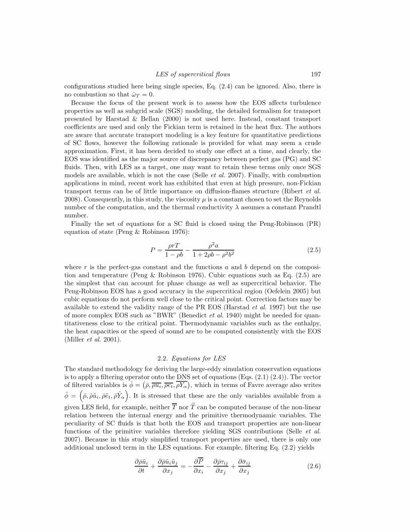
Figure 1. Schematic representation of the two configurations: (a) planar temporal jet, (b)Homogeneous Isotropic Turbulence.

Case name EOS Re Mach P (MPa) T (K) ρ (kg.m−3) Grid resolutionTJ hd PR 2187 0.15 3.97 127/300 433/45 2563

TJ d PR 2187 0.15 3.97 135/300 186/45 2563

TJ d PG PG 2187 0.15 3.97 135/300 99/45 2563

HITa PR 80 0.02/0.1/0.3 0.1 300 1.12 1283

HITb PR 80 0.02/0.1/0.3 4 300 45 1283

HITc PR 80 0.02/0.1/0.3 4 140 158 1283

Table 1. List of cases. All simulations are performed using pure nitrogen (Pc = 3.4 MPa,Tc = 126.2 K) in a cubic domain of arbitrary size L = 1 m with periodic boundary conditions.

In both configurations the domain is periodic in all three directions, which alleviates thequestion of boundary condition / turbulence interaction.

The initial conditions are prescribed with the input of the primitive variables (P , T ,ui). In all test cases, the initial pressure is uniform. For HIT, the initial temperatureis also uniform, whereas for TJ cases, the inner and outer streams can have differenttemperatures in order to generate a density variation. For the velocity, first the Machnumber is set (convective Mach number M0

c in the case of TJ and turbulent Mach numberM0

t in the case of HIT), then the functional form of the velocity field is prescribed asfollows:• HIT: a normalized fluctuation-velocity field with a Passot-Pouquet spectrum is built

using an external turbulence generator. This field is then multiplied by the prescribedMach number M0

t . The velocity reference for HIT is the root mean square of the wholefield, noted u′

HIT .• TJ: following the work of Papamoschou & Roshko (1988) and the correction for real-

gas effects described by Miller et al. (2001) the outer-stream (respectively inner-stream)axial velocity uout

1(respectively uin

1) is chosen so that the vortical structures resulting

from the shear-layer natural instability are stationary in the computational domain. Thevelocity reference for TJ cases is u′

TJ = (|uou1|+ |uin

1|)/2. The transition between the two

streams is performed using a combination of error functions with adjustable jet thicknessδ0

J and vorticity thickness δ0

ω. To reduce the integration time necessary to reach transition,the formation of vortices is seeded with an initial perturbation, which is a HIT velocityfield restricted to the inner stream with an intensity set to 10% of u′

TJ .


Finally, the global initial Reynolds number of the computation is set by choosing alength scale (initial jet thickness δ0

J for TJ and integral length scale L0

t for HIT) andimposing a constant viscosity µ.

4. Results and discussion

4.1. A priori study

The basic idea in an a priori study is to filter a DNS result and compute the exactSGS contributions, which can then be compared to their model counterpart based onthe filtered field (Piomelli et al. 1988). However, one should not expect the model tomatch the exact SGS contribution at each computational point or versus time. Indeed,SGS models can only be expected to perform in a looser statistical sense by providingthe adequate average dissipation to the resolved structures (Pope 2000). Two statisticaltools are used to measure the performance of a given model: the correlation and theleast-square fit between the model SGS and its exact DNS-extracted counterpart. Fora model to be acceptable, its correlation with the exact SGS contribution must be asclose to unity as possible. Once good correlation is established, the least-square fit is ameasure of the model coefficient.

In this study, it was decided to test three SGS models:• Smagorinsky (SM) model (Smagorinsky 1963), which is based on an eddy-viscosity

concept

τSMij −

1

3τSMkk δij = − (CSM∆)2 S

[Sij −

1

3Skkδij

](4.1)

where S =√

SijSij .• Gradient (GR) model (Clark et al. 1979), which is based on a Taylor series expansion

of the filtered variables

τGRij = CGR∆2

∂ui

∂xk

∂uj

∂xk

. (4.2)

• Scale Similarity (SM) model (Bardina et al. 1980), which assumes similarity betweenscales around the LES filter cutoff frequency

τSSij = CSS

(uiuj − ui

uj

)(4.3)

where the operator ( · ) denotes filtering at a length scale typically larger than the LESfilter ( · ).

The a priori study of these models has already been performed in previous work(Selle et al. 2007), though in slightly different configurations: two-species mixing layers.Therefore, this part of the present work may be seen as a further validation of previousresults. Indeed, for the single-species TJ and HIT cases scrutinized in this work, theconclusions were basically the same as those of Selle et al. (2007):• The Smagorinsky model shows quite poor performance in terms of correlation, typ-

ically lower than 0.25, as well as a wide spreading of least-square fit values over thecomponents of τij . This finding is not new (McMillian & Ferziger 1979; Liu et al. 1994)but one should also point out that the Reynolds number in typical a priori studies is notvery high and therefore not entirely consistent with the hypothesis of a fully turbulentflow with a wide inertial range.• Both GR and SS models show high correlation levels with a slight advantage for the

GR model.


In the interest of time, the use of a dynamic formulation for the model coefficient wasnot considered in the present work although it is known that dynamic models generallyoutperform their constant-coefficient versions.

4.2. DNS of temporal jets

The three TJ configurations presented in Table 1 match the experimental thermodynamicconditions of Mayer et al. (2003) for the pressure, temperature and composition (purenitrogen). The pressure is 3.97 MPa and the outer-stream temperature is T out

0= 300 K

in all cases. Using the PR EOS, two temperatures were tested for the inner stream:for case TJ hd, T in

0= 127 K, which leads to a very dense core, and for case TJ d,

T in0

= 135 K, which reduces the density by a factor of 2.3. Such sensitivity to a minorchange in temperature (9 K in the present case) is typical for fluids close to their criticalpoint. Then, one additional TJ case was computed to evidence the role of the EOS: casePTJ d PG duplicates case PTJ d except that it was performed with the perfect-gas EOSinstead of the PR EOS. The use of the PG EOS leads to a further decrease of a factor 1.8of the initial inner-stream density. Unfortunately, the experimental velocity and Reynoldsnumber could not be matched with the current grid resolution of 2563. The Mach numberwas set to 0.15 (compared to about 0.01 in the experiment) to improve the efficiency ofthe compressible solver, and a pseudo-viscosity was used to set the Reynolds number.The final difference with the experimental configuration of Mayer et al. (2003) is that aperiodic planar jet (Fig. 1 (a)) is computed instead of a round jet.

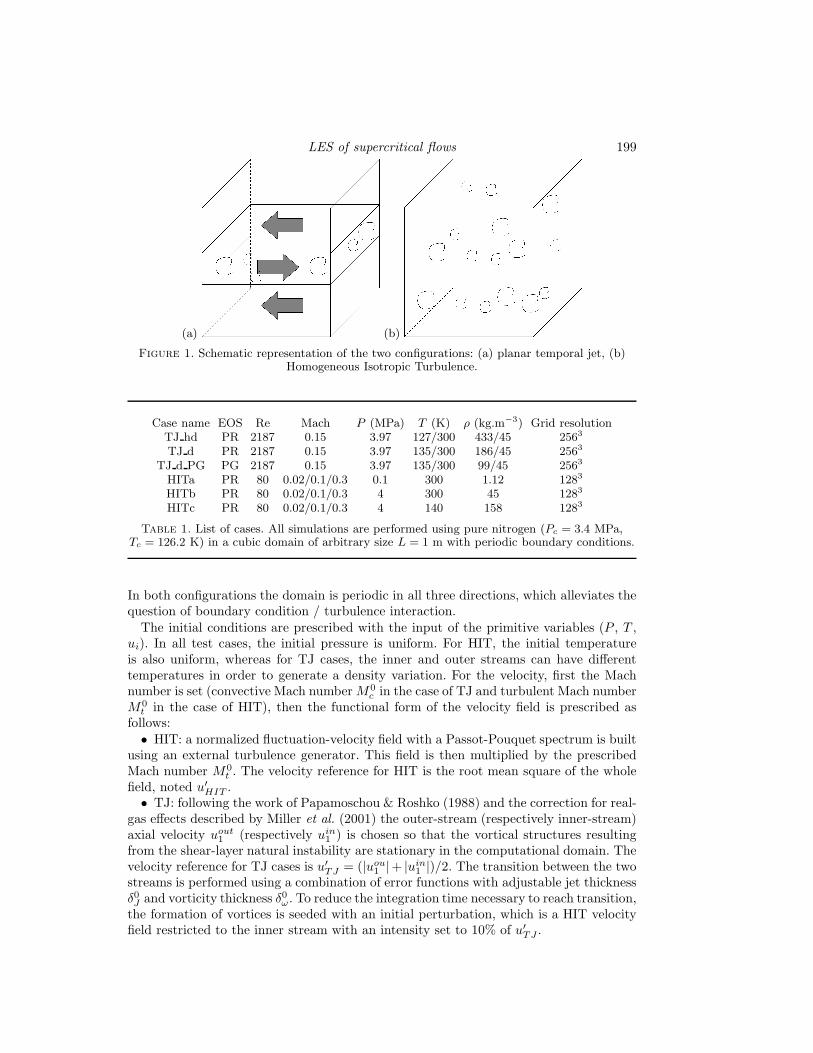
The qualitative influence of the EOS and the thermodynamic conditions is evidencedby plotting the density and the enstrophy in the middle cross-stream section (Fig. 2). Thestriking feature about the density fields in Fig. 2 (a, c, e) is that larger values in the innercore seem to stabilize the jet. Even though all cases display large vortical structures ofcomparable size, their penetration in the inner layer is damped by the density gradient.Case TJ hd (Fig. 2 (a)) also shows numerous finger-like structures typical of SC flowswhereas case TJ d PG (Fig. 2 (e)) displays smeared contours revealing efficient small-scale mixing. This observation is confirmed by the analysis of the enstrophy contours(Fig. 2 (b, d, f)) where it is obvious that the larger density in the inner stream ofcase TJ hd hinders the formation of small-scale structures within the flow. Large scaleshowever are not greatly affected. Small scales eventually proliferate in case PTJ hd (notshown) but it would seem that the large density difference has an impact on transitionmechanisms. This statement is further confirmed by the analysis of case TJ d PG (Fig. 2(f)), which exhibits even more small structures together with its smaller density ratio.

Because planar jets are homogeneous in the streamwise and spanwise directions, onecan define planar-averaged quantities at each cross-stream location. The correspondingoperator is denoted {·}. Then, one can define the turbulent velocity components as u′

i =ui − {ui} and the turbulent kinetic energy e′k = u′

iu′

i/2, which is a measure of thedevelopment of turbulent structures in the flow. Also, mixing efficiency is measured bythe ”mixture-fraction like” variable ZT = θ(1 − θ), where θ = (T − T in

0)/(T out

0− T in

0) is

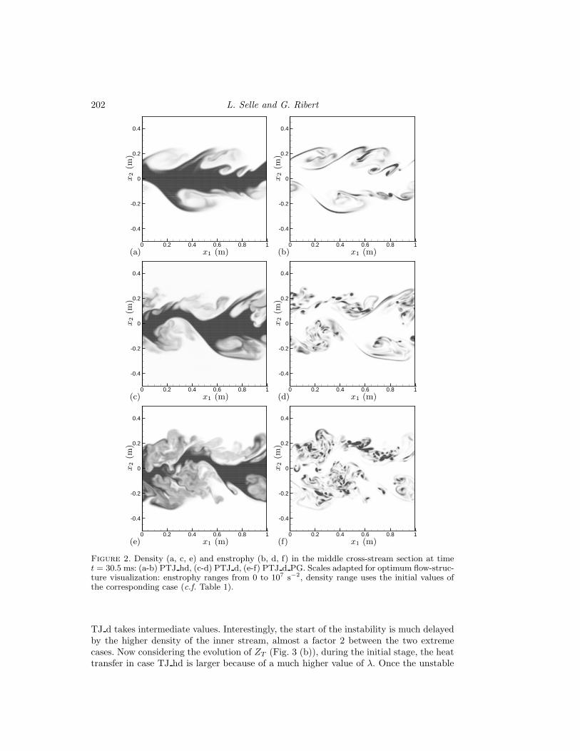
the reduced temperature. The two variables e′k and ZT allow a more quantitative viewof EOS and thermodynamic effects on turbulence properties and their domain-averagedtemporal evolution is represented in Fig. 3.

For all TJ configurations the initial perturbation intensity is quite small so that att = 0, 〈e′k〉 ≃ 0 (Fig. 3 (a)), where 〈·〉 denotes averaging over the whole computationaldomain. After a period of very slow increase, a sudden surge in 〈e′k〉 reveals the start ofthe natural mixing-layer instability eventually transitioning to turbulence. As depictedin Fig. 2, case TJ d has the lowest fluctuation level, case TJ d PG the highest, while


0 0.2 0.4 0.6 0.8 1

-0.4

-0.2

0

0.2

0.4

x1 (m)

x2

(m)

(a)0 0.2 0.4 0.6 0.8 1

-0.4

-0.2

0

0.2

0.4

x1 (m)

x2

(m)

(b)

0 0.2 0.4 0.6 0.8 1

-0.4

-0.2

0

0.2

0.4

x1 (m)

x2

(m)

(c)0 0.2 0.4 0.6 0.8 1

-0.4

-0.2

0

0.2

0.4

x1 (m)

x2

(m)

(d)

0 0.2 0.4 0.6 0.8 1

-0.4

-0.2

0

0.2

0.4

x1 (m)

x2

(m)

(e)0 0.2 0.4 0.6 0.8 1

-0.4

-0.2

0

0.2

0.4

x1 (m)

x2

(m)

(f)

Figure 2. Density (a, c, e) and enstrophy (b, d, f) in the middle cross-stream section at timet = 30.5 ms: (a-b) PTJ hd, (c-d) PTJ d, (e-f) PTJ d PG. Scales adapted for optimum flow-struc-ture visualization: enstrophy ranges from 0 to 107 s−2, density range uses the initial values ofthe corresponding case (c.f. Table 1).

TJ d takes intermediate values. Interestingly, the start of the instability is much delayedby the higher density of the inner stream, almost a factor 2 between the two extremecases. Now considering the evolution of ZT (Fig. 3 (b)), during the initial stage, the heattransfer in case TJ hd is larger because of a much higher value of λ. Once the unstable


0 0.01 0.02 0.030

50

100

150

200

Time (s)

〈e′ k〉

(m2.s

−2)

(a)0 0.01 0.02 0.03

0.00

0.02

0.04

0.06

0.08

0.10

Time (s)

〈ZT〉

(b)

Figure 3. Planar temporal jet: (a) averaged turbulent kinetic energy, (b) averaged mixingparameter. TJ hd, TJ d, case TJ d PG

modes of the jet develop, turbulent mixing becomes more efficient than laminar heattransfer so that the ranking becomes similar to that of 〈e′k〉.

One clear conclusion of this section: The use of the perfect-gas EOS does not only leadto incorrect values of the density or transport properties, which might be addressed bycorrection factors or tabulation, but also mis-predicts turbulence properties.

4.3. DNS of homogeneous isotropic turbulence

The case of decaying HIT is studied here to investigate the occurrence of local compress-ibility effects in SC fluids. Simulations are conducted for three thermodynamic conditions(c.f. Table 1) at three values of the Mach number (0.02, 0.1 and 0.3). The computationaldomain initially contains at least 10 integral length scales (Lt) for statistical convergenceof the velocity field, and the mesh size is less than two Kolmogorov scales for adequatedescription of small turbulence scales. After five turnover times τ = Lt/u′

HIT , the ve-locity field represents a realistic turbulent flow without any connection to the initialcondition. The 3-D energy spectrum were scrutinized, searching for an impact of thethermodynamic conditions. A first simulation is realized at standard conditions of pres-sure and temperature (HITa) in order to get a reference behavior of the decaying HIT.The pressure is then increased near the critical pressure of N2 (HITb) keeping the otherparameters constant, but no significant changes were observed. Finally, the temperatureis decreased to 140 K (case HITc) to come near the critical point of N2 reaching highdensity value. However, the impact of the proximity of the critical point on the kineticenergy seems to be negligible. Even at M = 0.3 no compressibility effect due to the EOSare observed.

Further investigation is still required for a definite conclusion about the HIT propertiesin SC fluids. The influence of the Mach number (if any) could be investigated as in Leeet al. (1991).

4.4. Large-eddy simulations

The LES of case TJ d was performed using the GR model. The initial condition for theLES is the DNS initial condition onto which a top-hat filter was applied. The resolutionwas decreased by a factor of 4 in all directions (i.e. 643 mesh). Figure 4 compares thetemperature fields of the filtered DNS with the LES result. While the larger structures ofthe flow as well as the overall expansion of the jet seem to be qualitatively well-predicted,the lack of small structures in the LES is striking. This observation is further confirmed


0 0.2 0.4 0.6 0.8 1

-0.4

-0.2

0

0.2

0.4

x1 (m)

x2

(m)

(a)0 0.2 0.4 0.6 0.8 1

-0.4

-0.2

0

0.2

0.4

x1 (m)

x2

(m)

(b)

0 0.2 0.4 0.6 0.8 1

-0.4

-0.2

0

0.2

0.4

x1 (m)

x2

(m)

(c)0 0.2 0.4 0.6 0.8 1

-0.4

-0.2

0

0.2

0.4

x1 (m)

x2

(m)

(d)

Figure 4. Temperature in the middle cross-stream section for case TJ d. (a, c) t = 26 ms and(b, d) t = 38 ms. (a, b) LES field, (c, d) filtered DNS on the LES mesh. Dark regions are cold(135 K) while bright zones are hot (300 K).

0 0.01 0.02 0.03 0.04 0.050

50

100

150

200

Time (s)

〈e′ k〉

(m2.s

−2)

Figure 5. Temporal evolution of averaged turbulent kinetic energy. DNS, filteredDNS, LES with gradient model

by the temporal evolution of 〈e′k〉 presented in Fig. 5. First the LES does not matchthe level of resolved fluctuations shown in the filtered DNS, but it also appears that theproduction of velocity fluctuations is delayed. This would not be beneficial in an actualLES of a spatial jet because a measure such as the jet-core length would be mis-predicted.


4.5. Considerations about the numerics

The numerics used in this study (Kennedy & Carpenter 1994) is stabilized with a tenth-order explicit filter. Two limitations for this choice were found for the present work:• Gibbs errors would occur when the resolution of the density gradient is poor. For

example, when doing the LESs, the resolution of the temperature (and therefore density)turned out to be more crucial than that of turbulent structures.• Robustness of the algorithm turned out to be quite sensitive to the filtering frequency

while dealing with SC conditions. Some computations had to be carried out with filteringoperations at each time step, which might be seen as a bit of a stretch given its initialpurpose of stabilization over long integration times.

Actually, these limitations are already noted in the conclusion of the original articleby Kennedy & Carpenter (1994). Other numerical schemes have not yet be tested buttwo main paths for improved robustness were identified:• A modification of the convective term for the energy equation such as proposed

by Honein & Moin (2004) could reduce numerical errors. Indeed, because of the strongnon-linearity of the PR EOS, the energy equation might be less stable than in PG solvers.• The use of implicit spatial differentiation and staggered formulation as described by

Nagarajan et al. (2003) seem to greatly improve the robustness and would be a goodcandidate for LES of SC flows.

5. Conclusion

This work presents an exploratory study of equation of state effects on turbulence undersupercritical conditions. DNS of single-species temporal jet and homogeneous isotropicturbulence were carried out using a Peng-Robinson EOS. It was found that some turbu-lence properties are affected by thermodynamic conditions. For the TJ configurations,strong density gradients seem to delay the formation of small-scale structures. For HITconfigurations, the analysis of the energy spectrum showed no significant influence of thethermodynamic conditions though more detailed investigation is required. The a priori

analysis of a selection of subgrid-scale models was conducted showing promising resultsfor LES. A posteriori results however revealed that the SGS dissipation was too great butmore importantly, the numerics lacked the sufficient robustness to accurately computethe high density gradients typical of SC flows.

Acknowledgments

The authors would like to thank Professor Senjiva Lele for fruitful discussions andfresh ideas about state-of-the-art numerical strategies for DNS and LES. The support ofthe Center for Turbulence Research and CINES (a French national computing center)for computational resources is gratefully acknowledged.

REFERENCES

Bardina, J., Ferziger, J. H. & Reynolds, W. C. 1980 Improved subgrid-scalemodels for large-eddy simulation. AIAA Paper (80-1357).

Bellan, J. 2000 Supercritical (and subcritical) fluid behavior and modeling: drops,streams, shear and mixing layers, jets and sprays. Prog. Energy Comb. Sci. 26 (4-6),329–366.


Benedict, M., Webb, G. B. & Rubin, L. C. 1940 An empirical equation for thermo-dynamic properties of light hydrocarbons and their mixtures. J. Chem. Phys. 8 (4),334–345.

Clark, R. A., Ferziger, J. H. & Reynolds, W. C. 1979 Evaluation of subgrid-scalemodels using an accurately simulated turbulent flow. J. Fluid Mech. 91, 1–16.

Graboski, M. & Daubert, T. 1978 A modified soave equation of state for phaseequilibrium calculations. Ind. Eng. Chem. Process Des. Dev. 18 (2), 443–448.

Harstad, K. & Bellan, J. 2000 An all-pressure fluid drop model applied to a binarymixture: Heptane in nitrogen. Int. J. Multiphase Flow 26, 1657–1706.

Harstad, K., Miller, R. & Bellan, J. 1997 Efficient high-pressure state-equations.AIChE Journ. 43 (6), 1605–1610.

Honein, A. E. & Moin, P. 2004 Higher entropy conservation and numerical stabilityof compressible turbulence simulations. J. Comput. Phys. 201, 531–545.

Keizer, J. 1987 Statistical Thermodynamics of Nonequilibrium Processes. New York:Springer.

Kennedy, C. A. & Carpenter, M. H. 1994 Several new numerical methods for com-pressible shear-layer simulations. Applied Num. Math. 14, 397–433.

Lee, S., Lele, S. K. & Moin, P. 1991 Eddy shocklets in decaying compressible tur-bulence. Phys. Fluids 3, 657–664.

Liu, S., Meneveau, C. & Katz, J. 1994 On the properties of similarity subgrid-scalemodels as deduced from measurements in a turbulent jet. J. Fluid Mech. 275, 83–119.

Lou, H. & Miller, R. S. 2001 On the scalar probability density function transportequation for binary mixing in isotropic turbulence at supercritical pressure. Phys.

Fluids 13 (11), 3386–3399.

Mayer, W., Telaar, J., Branam, R., Schneider, G. & Hussong, J. 2003 Ra-man measurements of cryogenic injection at supercritical pressure. Heat and Mass

Transfer 39, 709–719.

McMillian, O. J. & Ferziger, J. H. 1979 Direct testing of subgrid scale models.AIAA J. 17, 1340–1346.

Miller, R. S., Harstad, K. & Bellan, J. 2001 Direct numerical simulations ofsupercritical fluid mixing layers applied to heptane–nitrogen. J. Fluid Mech. 436,1–39.

Moureau, V., Lartigue, G., Sommerer, Y., Angelberger, C., Colin, O. &

Poinsot, T. 2005 High-order methods for dns and les of compressible multi-component reacting flows on fixed and moving grids. Journal of Computational

Physics 202 (2), 710–736.

Nagarajan, S., Lele, S. K. & Ferziger, J. H. 2003 A robust high-order compactmethod for large eddy simulation. J. Comput. Phys. 19, 392–419.

Oefelein, J. 2005 Thermophysical characteristics of shear-coaxial lox–hflames at su-percritical pressure. Proc. Combust. Inst. 30, 2929–2937.

Oefelein, J. 2006 Mixing and combustion of cryogenic oxygen-hydrogen shear-coaxialjet flames at supercritical pressure. Comb. Sci. Tech. 178 (1-3), 229–252.

Oschwald, M., Smith, J., Branam, R., Hussong, J., Schik, A., Chehroudi, B.

& Talley, D. 2006 Injection of fluids into supercritical environments. Combust.

Sci. and Tech. 178 (1-3), 49–100.

Palle, S., Nolan, C. & Miller, R. S. 2005 On molecular transport effects in realgas laminar diffusion flames at large pressure. Phys. Fluids 17 (10), 103601.


Papamoschou, D. & Roshko, A. 1988 The compressible turbulent shear layer: anexperimental study. J. Fluid Mech. 197, 453–477.

Peng, D.-Y. & Robinson, D. 1976 A new two-constant equation of state. AIChE

Journ. 15 (1), 59–64.

Piomelli, U., Moin, P. & Ferziger, J. H. 1988 Model consistency in large eddysimulation of turbulent channel flows. Phys. Fluids 31 (7), 1884–1891.

Pope, S. B. 2000 Turbulent Flows. Cambridge University Press.

Ribert, G., Zong, N., Yang, V., Pons, L., Darabiha, N. & Candel, S. 2008Counterflow diffusion flames of general fluids: Oxygen/hydrogen mixtures. Comb.

and Flame 154, 319–330.

Selle, L., Okong’o, N., Bellan, J. & Harstad, K. 2007 Modelling of subgrid-scalephenomena in supercritical transitional mixing layers: an a priori study. J. Fluid

Mech. 593, 57–91.

Smagorinsky, J. 1963 General circulation experiment with the primitive equations, i.the basic experiment. Mon. Weath. Rev. 91.

Zong, N., Meng, H., Hsieh, S. & Yang, V. 2004 A numerical study of cryogenic fluidinjection and mixing under supercritical conditions. Phys. Fluids 6 (12), 4248–4261.

Modeling requirements for large-eddy simulation of turbulent flows

Documents