Modeling Relationships among 217 Fires Using Remote ...

Remote Sens. 2011, 3, 2005-2028; doi:10.3390/rs3092005

Remote Sensing ISSN 2072-4292

www.mdpi.com/journal/remotesensing Article

Modeling Relationships among 217 Fires Using Remote Sensing of Burn Severity in Southern Pine Forests

Sparkle L. Malone 1, Leda N. Kobziar 1,*, Christina L. Staudhammer 1,2 and Amr Abd-Elrahman 3

1 School of Forest Resources and Conservation, University of Florida, Newins-Ziegler Hall, P.O. Box 110410, Gainesville, FL 32611, USA; E-Mail: [email protected]

2 Department of Biological Sciences, University of Alabama, 407 Biology Bldg, P.O. Box 870344, Tuscaloosa, AL 35487, USA; E-Mail: [email protected]

3 School of Forest Resources and Conservation, University of Florida, 1200 N. Park Road, Plant City, FL 33563, USA; E-Mail: [email protected]

* Author to whom correspondence should be addressed; E-Mail: [email protected]; Tel.: +1-786-489-1090; Fax: +1-250-348-1786.

Received: 20 July 2011; in revised form: 20 August 2011 / Accepted: 29 August 2011 / Published: 7 September 2011

Abstract: Pine flatwoods forests in the southeastern US have experienced severe wildfires over the past few decades, often attributed to fuel load build-up. These forest communities are fire dependent and require regular burning for ecosystem maintenance and health. Although prescribed fire has been used to reduce wildfire risk and maintain ecosystem integrity, managers are still working to reintroduce fire to long unburned areas. Common perception holds that reintroduction of fire in long unburned forests will produce severe fire effects, resulting in a reluctance to prescribe fire without first using expensive mechanical fuels reduction techniques. To inform prioritization and timing of future fire use, we apply remote sensing analysis to examine the set of conditions most likely to result in high burn severity effects, in relation to vegetation, years since the previous fire, and historical fire frequency. We analyze Landsat imagery-based differenced Normalized Burn Ratios (dNBR) to model the relationships between previous and future burn severity to better predict areas of potential high severity. Our results show that remote sensing techniques are useful for modeling the relationship between elevated risk of high burn severity and the amount of time between fires, the type of fire (wildfire or prescribed burn), and the historical frequency of fires in pine flatwoods forests.

OPEN ACCESS

Remote Sens. 2011, 3

2006

Keywords: burn severity; remote sensing; differenced normalized burn ratios; fire frequency; pine flatwoods forest; fire model; wildfire; prescribed fire

1. Introduction

In forests characterized by a historically frequent fire return interval, prescribed fire is often used as a tool to mimic the effects of natural fire. The absence of fire in such forests would cause significant changes in vegetative species structure and composition, and could increase the threat of large-scale wildfires. In pine flatwoods forests of the southern US, prescribed burns reduce fuel accumulations to minimize damage from potential wildfires [1,2], improve wildlife habitat, and conserve biodiversity [3-6]. However, implementing prescribed burns is increasingly difficult due to concerns related to the wildland urban interface (WUI). In particular, fire management decision-making in Florida has been shown to be dictated by urban encroachment, forest fragmentation, and the challenges associated with smoke management [7]. In WUI areas, fire behavior must be carefully controlled to prevent escapes. Managers strive to implement burns where fuel and weather conditions will minimize the potential for the high-severity fires that create challenges for smoke management and post-fire ecosystem recovery.

Fire severity is a measure of ecological and physical change attributable to fire [8,9], and is dictated by the intersection of fuels and weather conditions. In addition to being associated with smoke production, severity is an important post-fire metric used to explain fire effects on exotic species establishment, soil responses, and forest recovery. To describe fire effects in the southeastern US, burn severity is classified in four categories: unburned, low, medium, and high severity [10-13]. Low severity burns are characterized by lightly burned areas where only fine fuels are consumed with minor scorching of trees in the understory [14]. Areas of moderate severity retain some fuels on the forest floor and have crown scorching in mid-large trees with mortality of small trees [14]. High severity zones generally experience complete combustion of most of the litter layer, duff and small logs, mortality of small to medium trees, and consumption of large tree crowns [14].

Assessing burn severity across a frequently burned landscape can provide important information about both the immediate and longer-term consequences of fire use and management, as the severity of one fire likely influences the severity of the subsequent fire. The timespan between fire events can also have a significant effect on subsequent fire behavior and fire effects [1,2]. However, few studies have addressed the relationship between fire frequency, burn severity, and subsequent fire patterns in Florida’s fire-prone forests. Outcalt and Wade [2] found a significant relationship between the amount of time since last fire and tree mortality following a wildfire in Florida pine flatwoods [2]; as time increased to two or more years, mortality also increased [2]. Also in pine flatwoods, Davis and Cooper [1] showed that fuel accumulations of three years or less supported fewer fires, lower fire intensities, and lower burned acreage. These studies suggest that one fire affects the next, but do not address patterns across landscapes or among fires of differing severity, and are limited in temporal scope.

Combined with existing information about fire locations and perimeters, burn severity histories can be mapped to monitor trends in fire effects over time, in relation to frequency of fire, and as a function


2007

of time since last fire. Such data can then be used to make inferences about future fires. Remote sensing techniques are often utilized to monitor changes in fire regimes over time and to map burn severity [11,15,16], but the technique has been under-utilized for burn severity analysis in southern forests [15]. Normalized burn ratios (NBR) use the difference between Landsat Thematic Mapper (TM) near and mid-infrared band reflectance values to quantify the severity level of a burned area [14]. The difference between bands 4 and 7 reflectance values can be attributed to fire induced changes in soil moisture, canopy cover, biomass, charring, and exposed soil. Difference normalized burn ratios (dNBR) capture fire effects by differencing pre- and post-fire NBRs from ETM/TM images directly before and soon after a fire. Changes in green reflectance values are captured by band 4; while increases in charred fuels, exposed soil, and decreases in vegetation density cause an increase in band 7. The dNBR technique is effective in representing burn severity because it captures relative changes in the pre- and post-fire normalized burn ratio. Employed as a radiometric index, dNBRs can be directly related to burn severity [14,16] and, as long as the fire is within the resolution range of the satellite sensor (30 m), fires and their associated burn severity are often detectable [17,18].

Previous studies in other regions have used dNBRs to calibrate severity levels to specific forest types [10,15,16,19], compare severity levels between fire events [12,19], interpret the effects of fuel management techniques on severity levels [20], and to monitor changes in vegetation over time [17,21] and across topography [11,22]. The multi agency project, Monitoring Trends in Burn Severity (MTBS) is currently using dNBRs to map burn severity and the perimeters of wildfires greater than 405 ha in the western US and 202 ha in the eastern US [23]. The MTBS does not, however, compare a given fire’s severity to the severity of subsequent fires, and given that most fires in southern states are less than 202 ha in size, many fires are overlooked.

Here, we analyze a decade of wildfire and prescribed burn severities in Florida flatwoods pine forests using dNBR, and examine whether landscape, vegetation, soils, and fire history, and fire frequency influence burn severity patterns. We then use these relationships to derive predictive models for high severity prescribed burns and wildfires. We hypothesize that time-since-fire will influence the probability of high burn severity in pine flatwoods only so long as the vegetation recovery does not result in altered species composition and structure. Severity should increase as time and fuel loads increase up to that threshold. We also hypothesize that mesic communities will have a higher probability of high burn severity than hydric communities during prescribed burns, while the opposite could be observed for wildfires. Prescribed burns are most frequently administered when hydric communities (e.g., cypress domes) are moist, as these communities are fire-sensitive. Because of this, prescribed burns only partially consume these understory fuels, with little consumption of the duff layer [2] resulting in overall low severity. Consequently, hydric areas accumulate heavy fuel loads that can only support combustion during extended drought periods, and most often burn under weather conditions conducive to large, high-intensity wildfires [1]. Research has shown that the number and size of wildfires in Florida are positively correlated with drought conditions [24].

Optimally, prescribed burns in these forests are administered for minimal overstory mortality and partial consumption of understory surface fuels, with little consumption of the ground fuels including the duff layer. Predicting the probability of high severity wildfire risk would benefit land managers in their wildfire mitigation planning and tactics. There exist few locations worldwide where multiple prescribed burns and wildfires occur and overlap from one year to the next. The convergence of


2008

frequent prescribed fire and fast vegetation recovery rates sets the stage for this unique opportunity. Understanding how and why one fire affects a subsequent fire can lend insight into the complex relationships between fire behavior, fuels and vegetation recovery, and burn severity over time, and expand the utility of remotely sensed imagery for ecological research.

2. Methods

2.1. Study Site

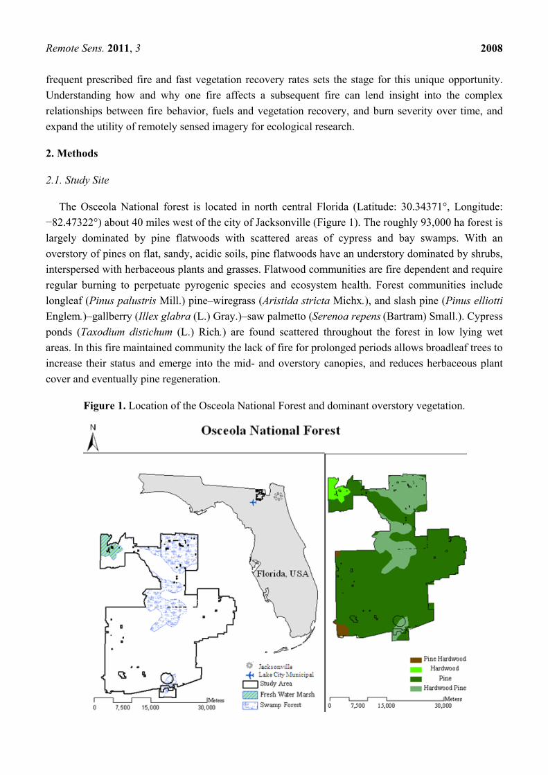
The Osceola National forest is located in north central Florida (Latitude: 30.34371°, Longitude: −82.47322°) about 40 miles west of the city of Jacksonville (Figure 1). The roughly 93,000 ha forest is largely dominated by pine flatwoods with scattered areas of cypress and bay swamps. With an overstory of pines on flat, sandy, acidic soils, pine flatwoods have an understory dominated by shrubs, interspersed with herbaceous plants and grasses. Flatwood communities are fire dependent and require regular burning to perpetuate pyrogenic species and ecosystem health. Forest communities include longleaf (Pinus palustris Mill.) pine–wiregrass (Aristida stricta Michx.), and slash pine (Pinus elliotti Englem.)–gallberry (Illex glabra (L.) Gray.)–saw palmetto (Serenoa repens (Bartram) Small.). Cypress ponds (Taxodium distichum (L.) Rich.) are found scattered throughout the forest in low lying wet areas. In this fire maintained community the lack of fire for prolonged periods allows broadleaf trees to increase their status and emerge into the mid- and overstory canopies, and reduces herbaceous plant cover and eventually pine regeneration.

Figure 1. Location of the Osceola National Forest and dominant overstory vegetation.


2009

Fire management and use in the Osceola National Forest is quite active, with an annual prescribed burning quota of over 13,000 ha. The majority of the forest is prescribed burned at a frequency of every 2–5 years. There are also sensitive areas within the forest that are not currently and actively managed by fire. Fire prescriptions are determined on a compartment level based on the current forest type and the desired future condition of the compartment. Osceola fire managers are challenged to meet federal quotas for prescribed burning each year, which require burning large areas within the handful of days that meet prescribed fire weather conditions. Sensitive areas near the forest like Lake City Municipal Airport, US Interstate Highway 10, and the nearby City of Jacksonville, provide additional challenges for fire managers (Figure 1).

2.2. Image Analysis

NBR raster GIS layers extracted from geometrically and radiometrically corrected Landsat 7 ETM and Landsat 5 TM imagery were downloaded through the United States Geological Survey (USGS) global visualization website [25]. Pre-processing steps for all images were conducted by the USGS EROS Data Center [23,26,27]. Scenes closest to the date of the fire (within the same season) were used for pre-fire images. Post-fire images were closest to the one-year anniversary of the fire (within the same season of the fire). The NBRs (Equation (1)) were computed as a normalized difference of the Landsat (ETM/TM) reflectance values from band 4 (B4; near-infrared band) and 7 (B7; mid-infrared band). The dNBR was computed using pre- and post-fire event NBR to quantify burn severity using Equation (2):

(1)

_ _ (2)

The dNBR can range from −2,000 to 2,000 yet typically range from −500 to 1,200 [28]. Negative values represent vegetation regrowth whereas positive values represent burn severity. Values close to zero are unburned areas and burned areas are generally greater than 100. The threshold between burned and unburned areas can range anywhere from 80 to 100 [27] depending on forest type.

2.3. Severity Classification

We used the 101 prescribed burns and 116 documented wildfires greater than 0.4 ha in size that occurred during the period from 1998 to 2008 to create a complete fire history for the entire forest using dNBRs for each fire event. General severity levels provided by the United States Geological Survey (USGS) [29] were reclassified into four severity levels to combine classes that result in similar fire effects; unburned (dNBR −100 to 99), low severity (dNBR −500 to −101, 100 to 269), moderate severity (dNBR 270 to 439), and high severity (dNBR 440–1,300) (Table 1). Burn severity level thresholds are within the thresholds for pine flatwoods and depression swamps developed by Picotte and Robertson 2011 [19]. Picotte and Robertson used 731 ground-level CBI plots for pine flatwoods forest and depression swamps on the Apalachicola National Forest, the Okefenokee National Wildlife Refuge, and the Osceola National Forest to develop burn severity thresholds. Unlike Picotte and Robertson 2011, we combined the re-growth burn severity class (dNBR −500 to −101) with the low


2010

severity class to distinguish burned from unburned areas in the model (Table 1). We also used a single set of severity thresholds for all forest types. A relativized version of the dNBR is often used to adjust the dNBR value according to the pre-fire NBR to correct for the variance in the reflectance of the initial plant cover types. However, we did not use this method. Picotte and Robertson 2011 found no added advantage with using the RdNBR method over the dNBR approach in pine flatwoods forest. To account for temporal variation in phenology and surface moisture conditions in the pre- and post-fire images, the mean value of unchanged forested pixels outside the burned areas were subtracted from the dNBR [12,28]. DNBRs were then clipped using fire perimeter shape files provided by the USDA Forest Service Osceola National Forest. Next, fires were merged to create a map that represented fire events for each year.

Table 1. Description of burn severity thresholds used to define severity classes (unburned, low, moderate, and high).

USGS Severity Class Reclassified Severity Class

DNBR range USGS Description Description

−100 to +99 Unburned within a fire perimeter Unburned

−500 to −101 Re-growth Low Severity

+100 to +269 Low Severity

+270 to +439 Low-Moderate Severity Moderate Severity

+440 to +659 Moderate-High Severity High Severity

+660 to +1,300 High Severity

Fire events were used to analyze the relationship between severity level of a previous fire and changes in the severity level of the next fire by time interval. An additional analysis quantified the relationship between fire history metrics for the entire forest and the likelihood of high burn severity in a given year. The layers created for each year (see figure in Section 3.6) in addition to forest community and forest type data were used to calculate covariates for use in the statistical model. Specifically, the fire layers were used to calculate: (1) latest severity level, which defines the burn severity level of the last fire event; (2) frequency, which is the number of times a pixel has burned within the dataset; and (3) time since last fire, which is the number of years since last fire. Calculations were made using the raster calculator in the ArcGIS spatial analyst extension software (ESRI, Redlands, CA, USA).

2.4. Model Development

Models were created to investigate the effects of fire history and environmental conditions on the probability of subsequent fire and its severity. Thus, models examined the occurrence of subsequent fires in a particular pixel (an initial or first fire, versus a second or subsequent fire). Four logistic models were estimated to evaluate the effects of the severity of the initial fire, the Palmer Drought Severity Index (PDSI) [30], fire type (wildfire or prescribed fire), forest type, community type and time since the initial fire on the probability of: (1) the occurrence of subsequent high burn severity;


2011

(2) burn severity increasing from the first to the second fire; (3) burn severity decreasing from the first to the second fire; and (4) repeated fire (of any severity level) during the study period (Table 2). Forests types were classified as pine, hardwood, hardwood-pine, or pine-hardwood forest types (Figure 1), and hydric or mesic community types. Forest type and community type were obtained from the Florida Geographic Data Library [31]. The forest type layer was developed by the University of Florida Geoplan Center. Vegetative communities were distinguished based on Davis [32]. Swamps, marshes, and other areas classified by the National Hydraulic Dataset as having standing water were classified as hydric and the rest of the forest was classified as mesic based on soil and forest types. Average PDSIs were computed for four calendar years: the year before and the year of the first fire, and the year before and the year of the second fire. Using calendar years as breakpoints for PDSI means that the fall/winter dry period is included in the PDSI average for the year before a fire.

Table 2. Independent variable inputs to models of subsequent fire and severity (all first-order interactions were also considered).

Models 1–4

Severity Level of the Initial Fire (Low, Moderate, or High Burn Severity)

Palmer Drought Severity Index (−4 to +4)

Fire Type (Wildfire or Prescribed Burn)

Forest Type (Pine, Hardwood, Pine-Hardwood, or Hardwood-Pine)

Community Type (Hydric or Mesic)

Time since the initial Fire (1 to 10 years)

Model 5

Severity Level of the Initial Fire (Low, Moderate, or High Burn Severity)

Palmer Drought Severity Index (−4 to +4)

Fire Type (Wildfire or Prescribed Burn)

Forest Type (Pine, Hardwood, Pine-Hardwood, or Hardwood-Pine)

Community Type (Hydric or Mesic)

Time since the initial Fire (1 to 10 years)

Fire Frequency (0.1 to 1)

We also developed a fifth model to investigate the relationship between the probability of experiencing high severity prescribed burns and wildfires and fire frequency in addition to the above-mentioned factors, and to use as a basis for testing model predictions. Fire frequency was computed as the total number of fires divided by the number of years of the entire study period. The first four logistic models were based on data from all wildfires and prescribed burns >0.4 ha in size from 1998 to 2008 on the Osceola National Forest. All areas that were within fire perimeters were included in this analysis. Each pixel was treated as one observation. Only the first and second fires during the


2012

observation period were used in this analysis to represent the time between fires. Approximately 40,469 ha were included in the dataset.

For the fifth model, fire history was developed for pixels using data up to 2005, and this data was then used to estimate the probability of exhibiting high burn severity effects in year 2006. The model was then tested against actual fire patterns for a specific year when multiple fires occurred. Model predictions were validated by comparing actual dNBRs for prescribed fire and wildfire that occurred in 2007. Probability of experiencing high burn severity was computed and presented spatially using the parameters estimated from the fifth logistic regression model. Model inputs were organized into individual layers and calculations were made using the raster calculator in the ArcGIS spatial analyst extension (ESRI, Redlands, CA, USA). The spatial model output showed the probability of a given area in the landscape displaying high burn severity for either prescribed burns or wildfires.

2.5. Logistic Regression Analysis

Logistic regression methods were utilized to determine fire probabilities as described by models 1–5 for both prescribed burns and wildfires, on a pixel level. Responses are coded as 1 or 0 for “success” or “failure”. For model 1, this corresponds to a pixel being burned or unburned, respectively, at the high severity level: 1,0, (3)

where is a realization of a random variable Yi that can take on the values of 1 and 0 with probabilities πi and 1 − πi. The variable Yi has a Bernoulli distribution with mean and variance depending on the underlying probability πi such that E(Yi) = πi and var(Yi) = πi(1 − πi). The probability, πi, is a linear function of a matrix of observed covariates, xi, transformed via the logit function to remove range restrictions: logit log 1 ′ (4)

where β is a vector of unknown parameters to be estimated. The logit maps probabilities from the range [0, 1] to the space of all real numbers [−∞, ∞]. Negative logits represent probabilities below 50% and positive logits represent probabilities above 50%. Solving for the probability of success requires exponentiating the logit and calculating the odds of success:

′1 ′ (5)

Maximum likelihood methods were used for parameter estimation. With this approach, parameters are estimated iteratively until parameters that maximize the log of the likelihood are obtained. Goodness of fit statistics, Akaike’s information criteria (AIC) and Bayesian information criteria (BIC), were used to compare competing models. AIC and BIC are model selection statistics that facilitate comparisons between models with different numbers of parameters. Both avoid increasing the likelihood by over fitting, measuring how close fitted values are to true values, with a penalty for the number of parameters in the model [33]. The ratio of the Pearson chi-square statistic to its degrees of freedom was used to determine if the model displayed lack of fit [29]. Values closer to 1 indicate that


2013

models fit the data well [33]. Since raster data is comprised of adjacent pixels, the assumption of independence among observations was likely violated due to spatial autocorrelation. Therefore, a generalized linear mixed model, which would model the spatial correlation directly, would be the most appropriate model. In theory, this could be accomplished using the SAS procedure PROC GLIMMIX, adding an appropriate spatial correlation structure. However, due to the volume of data involved, it is not possible to estimate this model without the aid of a super computer. Instead, random residuals were modeled to account for overdispersion [34].

A modified backward selection method was used to determine the appropriate covariates for the final model. First, all parameters were included in the model, including all first-order interactions between parameters. Then, the least significant covariates based on the Wald chi-square statistics were dropped one at a time until all covariates remaining in the model were significant (P < 0.05). At each step in model selection, not only was the significance of each model parameter evaluated, but we also ensured that the final model had the lowest AIC and BIC values. To test for differences among categorical levels, least square means were produced and differences were tested via the post-hoc Tukey-Kramer method.

3. Results

3.1. Predicting the Occurrence of Subsequent High Burn Severity

Based on the dNBR analysis of fire events over time, severity level of the first fire, PDSI for the year of the first and second fire, fire type for the second fire, community type, and the time interval between the first fire and the second fire were all significant indicators of high burn severity occurring subsequently. The overall model (P < 0.05) and the parameters were significant based on their Wald chi-square statistics (P < 0.05). The ratio of the Pearson chi-square statistic to its degrees of freedom was approximately 1.15, indicating good model fit (Table 3(a)).

As the severity level of the first fire increased, the probability of high burn severity in subsequent fire also increased, but the influence was weak. Areas previously burned at a high burn severity had the highest probabilities for high burn severity in subsequent fire while areas previously burned by low burn severity had the lowest probabilities (Table 3(a)). Areas previously burned by wildfires and hydric areas had higher probabilities of high burn severity in subsequent fire than areas that were prescribed burned and mesic areas (Table 3(a)). In hydric areas, the probability of high burn severity in areas burned previously by wildfires was 9.3% higher than in areas that were prescribed burned. In mesic areas, the probability of high burn severity in areas burned previously by wildfires was 13.72% higher than in areas that were prescribed burned. The probability of high burn severity in subsequent fire increased with the time interval between the first and second fire up to five to six years, then declined with time interval between fires seven to eight and nine to ten years (Table 3(a), Figure 2(a)).


2014

Table 3. Parameter estimates and their respective standard errors, and p-values for the regression models predicting the probability of: (a) high burn severity occurrence; (b) increasing in burn severity from one fire to the next; (c) decreasing in burn severity from one fire to the next; and (d) subsequent fire occurrence based on satellite imagery severity classifications from 1998 to 2008.

Parameter Model (a) Model (b) Model (c) Model (d)

Estimate Std. Error Estimate Std.

Error Estimate Std. Error Estimate Std.

Error P-value

Intercept −5.34 0.12 −1.31 0.03 1.15 0.03 1.22 0.02 <0.0001

Fire 1 Severity

Unburned 2.97 0.02 −0.73 0.02 <0.0001 Low −0.35 0.03 0.75 0.02 −2.89 0.02 −0.57 0.02 <0.0001

Moderate −0.20 0.03 Reference −1.19 0.03 −0.35 0.02 <0.0001 High Reference Reference Reference <0.0001

Fire 1 Type Wildfire 1.19 0.02 −0.51 0.01 0.29 0.01 <0.0001 Prescribed burn Reference Reference Reference

Fire 2 Type Wildfire 0.09 0.01 0.09 0.01 −1.02 0.03 <0.0001 Prescribed burn Reference Reference Reference

Time Interval Between Fires (Years)

1–2 1.68 0.11 −1.54 0.02 0.58 0.02 −0.61 0.02 <0.0001 3–4 0.45 0.12 −0.76 0.02 0.66 0.02 −0.79 0.02 <0.0002 5–6 4.66 0.12 0.22 0.03 −0.57 0.03 1.19 0.02 <0.0001 7–8 2.05 0.12 −1.53 0.02 0.72 0.03 0.17 0.02 <0.0001

9–10 Reference Reference Reference Reference

Forest Type Hydric 0.21 0.12 <0.0001 Mesic Reference <0.0001

Palmer Drought Severity Index

Average for the year before the first fire 0.65 0.01 <0.0001

Average for the year of the first fire 0.23 0.01 0.07 0.00 -0.47 0.01 <0.0001 Average for the year before the second

fire 0.48 0.00 -0.25 0.01 <0.0001

Average for the year of the second fire −0.09 0.01 -0.08 0.00 -0.03 0.00 <0.0001

Interaction Between Time Interval Between Fire 1 and Fire 2 (Years) and Fire Type 2

1–2 Wildfire 1.30 1.30 <0.0001 Prescribed burn Reference

3–4 Wildfire 0.13 0.13 <0.0005 Prescribed burn Reference

5–6 Wildfire 1.95 1.95 <0.0001 Prescribed burn Reference .

7–8 Wildfire −1.27 −1.27 <0.0001 Prescribed burn Reference

9–10 Wildfire Reference Prescribed burn Reference

Residual 1.15 0.96 0.98 1.00


2015

3.2. Probability of Burn Severity Increasing from the First to the Second fire

Severity level of the first fire, average PDSI values, fire type (prescribed or wildfire) of both the first and the second fire, and the time interval between the first and second fire were all significant indicators of the probability of increasing burn severity. The overall model was significant (P < 0.05) and the parameters were significant based on their Wald chi-square statistic (P < 0.05). The ratio of the Pearson chi-square statistic to its degrees of freedom was approximately 0.96, indicating good model fit (Table 3(b)). The severity level of the first fire and the probability of increasing subsequent burn severity were inversely related. Areas previously unburned within fire perimeters had the highest probabilities of increasing burn severity (73–83%) followed by areas previously burned at a low burn severity level (23–35%) and at a moderate burn severity level (12–20%) (Table 3(b)). The PDSI value for the year immediately prior to the second fire had the greatest influence on subsequent increasing burn severity, suggesting that fall/winter drought conditions were positively associated with increasing burn severity during the spring/summer season (Table 3(b)). Areas that burned as wildfires in the first fire had a lower probability of increasing subsequent burn severity versus those that burned in prescribed fire in the first fire. Areas burned by wildfires in the second fire had higher probabilities of increasing burn severity. On average, areas that were first burned by wildfires had a 7% lower probability of increasing subsequent burn severity versus that of prescribed burns. When the time interval was five to six years between fires, probability of increasing burn severity in subsequent fire was highest (ranging from 91–96%, depending on fire type), while the lowest probability of increasing burn severity (73–83% depending on fire type) occurred when there was one to two years between fires (Table 3(b); Figure 2(b)).

3.3. Probability of Burn Severity Decreasing from the First to the Second Fire

The regression model for the probability of decreasing burn severity in a subsequent fire included severity level of the first fire, average PDSI for the year before and the year of both the first and subsequent fires, fire type for both the first and second fire, and time interval between the first and second fire (Table 3(c)). The overall model was significant (P < 0.05) and the parameters were significant based on their Wald chi-square statistic (P < 0.05). The ratio of the Pearson chi-square statistic to its degrees of freedom was approximately 0.98, indicating good model fit (Table 3(c)). The probability of decreasing in severity level in subsequent fire was higher for areas that had previously exhibited high burn severity (93–94%) than those that had burned at moderate (80–85%) and low burn severity (42–52%) (Table 3(c)). Areas burned by wildfires in the first fire had higher probabilities of decreasing subsequent burn severity than areas that were prescribed burned in the first fire (Table 3(c); Figure 2(c)). On average, the probability of decreasing subsequent burn severity in areas that burned as wildfires was 5.5% lower than that of areas that were prescribed burned. The probability of decreasing in severity level in subsequent fire was the lowest for the time interval five to six years (ranging from 19–24%). All other time intervals had similar probabilities (30–50%) (Figure 2(c)).


2016

Figure 2. The relationship between time since last fire and: (a) the probability of high burn severity; (b) the probability of increasing burn severity; (c) the probability of decreasing burn severity; and (d) the probability of fire occurrence in subsequent fire by fire type.

3.4. Probability of Repeated Fires during the Study Period

The following indicators were significant in predicting the probability of a second fire occurrence during the study period:, the severity level of the first fire, fire type of the second fire, time interval between fires, and the interaction of time between fires and the second fire’s type (Table 3(d)). The overall model was significant (P < 0.05) and the parameters were significant based on their Wald chi-square statistic (P < 0.05). The ratio of the Pearson chi-square statistic to its degrees of freedom was approximately 1.00, indicating good model fit (Table 3(d)). As the burn severity level of the first fire increased, the probability of subsequent burning increased as well. Areas previously showing high burn severity had a 83–94% chance of burning, compared to areas previously showing low burn severity, which had a 70–76% probability. There was a higher probability of subsequent burning by wildfire than by prescribed fire (Table 3(d); average difference 13%, depending on previous fire type). Areas that had a time interval of five to six years between fires had the highest probability of burning (93–97%) (Figure 2(d)). The probability of burning was between 34 and 83% for all other time intervals (depending on fire type), generally increasing with time (Table 3(d), Figure 2(d)).

0

20

40

60

80

100

1-2 3-4 5-6 7-8 9-10

Prob

abili

ty o

f Hig

h B

urn

Seve

rity

(%)

Wildfire (Hydric Forest)

Wildfire (Mesic Forest)

Prescribed Burn (Hydric Forest)

Prescribed Burn (Mesic Forest)

0

20

40

60

80

100

1-2 3-4 5-6 7-8 9-10Prob

abili

ty o

f B

urn

Seve

rity

Incr

easi

ng (%

)

Time interval between fires (years)

Wildfire (Fire 1) Wildfire (Fire 2)

Prescribed Burn (Fire 1) Prescribed Burn (Fire 2)

0

20

40

60

80

100

1-2 3-4 5-6 7-8 9-10Prob

abili

ty o

f B

urn

Seve

rity

Dec

reas

ing

(%)

Wildfire (Fire 1) Wildfire (Fire 2)

Prescribed Burn (Fire 1) Prescribed Burn (Fire 2)

0

20

40

60

80

100

1-2 3-4 5-6 7-8 9-10

Prob

abili

ty o

f Fire

Occ

urre

nce

(%)

Time interval between fires (years)

Wildifire Prescribed Burn

a. c.

b. d.


2017

3.5. Temporal Thresholds and the Importance of Fire Type

The four models described above identify important thresholds for fire return intervals in pine flatwood forests. The time interval of five to six years between fires emerged as the point where previous fires had limited mitigating effects on subsequent fires. The probability of subsequent high burn severity was highest when the time interval was five to six years between fires (ranging 64–88%) for both prescribed burns and wildfires (Figure 2(a)). This interval was also associated with the highest probability of increasing in burn severity in subsequent fires, the lowest probability of decreasing burn severity (19–25%), and the highest probability of subsequent fire occurrence (93–97%) (Figure 2(b–d)). The models also identified three to four years between fires as an interval where previous fire activity reduced the probability of subsequent high burn severity and increased the probability of lower subsequent burn severity, but increased the severity of subsequent fires. Areas that remained unburned greater than six years also showed a mitigating effect on the probability of increasing burn severity in subsequent fires.

Areas that burned as wildfires had higher probabilities for high burn severity (9% higher on average) than did areas of prescribed burns. Yet, areas that were first prescribed burned had higher probabilities for the second fire increasing in severity level (27% higher on average) than wildfire burned areas. Areas previously burned by prescribed fire also had slightly higher probabilities for increasing burn severity level in subsequent fires than areas that were burned by wildfires. The probability of decreasing burn severity was slightly lower for areas that had been previously prescribed burned (6% lower on average) than for areas previously burned by wildfire. Hydric forests had higher probabilities of high burn severity (~1% higher on average) than did mesic forests.

3.6. Creating the Predictive Model to Use for Testing Known Fire Patterns

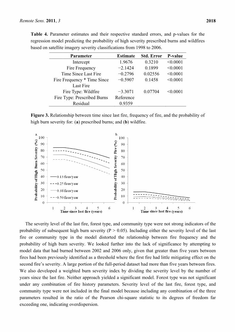
Based on the time series analysis of satellite imagery from 1998 to 2006, fire frequency, time since last fire, the interaction between frequency and time since last fire, and fire type were all significant predictors in the model for both high burn severity in prescribed burns and wildfires (Table 4). The overall model was significant (P < 0.05) and the parameters were significant based on their Wald chi-square statistic (P < 0.05). The ratio of the Pearson chi-square statistic to its degrees of freedom was approximately 0.94, indicating good model fit.

The model predicts that the majority of the forest (96%) in 2006 had a probability of high burn severity less than 75%. Time since last fire had a negative relationship with the probability of high burn severity for prescribed burns and wildfires; as time since last fire increased, the probability of high severity prescribed burns and wildfires decreased (Figure 3(a,b)). Also exhibiting a negative relationship with the probability of high burn severity, as frequency of fire increased, the probability of experiencing a high burn severity decreased (Figure 3(b)).

R

pfpmfsWyucpe

Remote Sens

Table regresbased

Figurehigh b

The seveprobability ofire or comprobability model data fires had beesecond fire’sWe also devyears since tunder any ccommunity parameters exceeding on

s. 2011, 3

4. Paramesion model on satellite

TFire F

FFire T

e 3. Relatioburn severity

rity level ofof subseque

mmunity typof high burthat had buen previouss severity. Aveloped a wthe last firecombinationtype were nresulted inne, indicatin

eter estimatpredicting imagery se

ParameInterce

Fire FrequTime Since LFrequency *

Last FiFire Type: WType: Presc

Residu

nship betwey for: (a) pr

f the last firent high burpe in the mrn severity.urned betwesly identifieA large portweighted bue. Neither apn of fire hnot included

n the ratio ng overdisp

es and theithe probabi

everity class

eter ept uency Last Fire * Time Sincire Wildfire cribed Burnual

een time sinrescribed bu

re, forest typrn severity model disto. We lookeeen 2002 and as a threstion of the furn severitypproach yieistory paramd in the finof the Pea

persion.

ir respectivility of highsifications fr

Estim1.96−2.14−0.27

ce −0.59

−3.30s Refere

0.93

nce last fire,urns; and (b

pe, and com(P > 0.05).orted the r

ed further innd 2006 onshold wherefull-period dy index by elded a signmeters. Seval model be

arson chi-sq

ve standard h severity pfrom 1998 to

mate Std.676 0.424 0.796 0.0907 0.

071 0.0ence 59

, frequency ) wildfire.

mmunity typ. Including relationshipnto the lackly, given th

e the first firdataset had dividing th

nificant modverity levelecause incluquare statis

errors, andrescribed bo 2006.

. Error P3210 <1899 <

02556 <1458 <

07704 <

of fire, and

pe were noteither the s

p between k of signifihat greater tre had little more than f

he severity del. Forest tl of the lasuding any cstic to its d

d p-values urns and w

P-value 0.0001 0.0001 0.0001 0.0001

0.0001

d the probab

t strong indiseverity levfire frequeicance by athan five yemitigating

five years blevel by thtype was nost fire, forecombinationdegrees of

201

for the wildfires

bility of

icators of thvel of the lancy and th

attempting tears betweeeffect on th

between firehe number oot significanest type, ann of the thre

freedom fa

18

he ast he to en he es. of nt nd ee far

R

3

2pfcrcmfs8(

sg

Remote Sens

3.7. Testing

In order t2007 was cpatterns acrofor prescribclassificationeflects the

could have bmore land wfires, the maseverity (0.5849 ha) with30%; 375 h

Figurefires inseverit

Model prseverity basgreater than

s. 2011, 3

the Predict

to examinechosen, as oss the landbed burns n of unburnburn severibeen missed

was burned bajority of th5%; 8 ha). h low levelsha) burned a

e 4. The obn the Osceoty for prescr

redictions fsed on fire n 75% were

tive Model a

the accuraboth prescr

dscape wereand 5,544

ned ha is baity for the ed. If the unby prescribe

he burned arThe major

s of high buat the moder

bserved burnola Nationalribed burns

for 2007 idehistory for selected as

against Kno

acy of the pribed and we heterogene

unburned ased on theentire inclu

nburned heced burns (~reas had lowrity of land urn severityrate burn se

n severity lel Forest, FL and wildfir

entified areacombined

s those exp

own Fire Pa

predictive mwildfire acteous with 4hectares w

e assumptionuded acreagtares are su1,771 ha) thw burn seve

burned byy in wildfireeverity level

evels for (aL versus (b)res.

as that had prescribed ected to bu

atterns

model againstivity was

472 ha of unwithin perin that the L

ge, and a smubtracted frohan by wilderity (84%; y wildfires es (0.14%; 2l compared

) the actual) Model der

increased pburns and

urn severely

st actual firwidespread

nburned areimeters forLandsat ETMmaller burneom the perifires (~1,221,497 ha) wwas also lo2 ha). A larto prescribe

l area burnerived probab

probability wildfires. A

y if a fire ev

re data for ad. In 2007,ea within firr wildfires. M/TM 30 ×ed area withimeter-base25 ha). Of thwith very litow burn serger portioned burns (14

ed during thbility of hig

of exhibitinAreas with vent were t

201

a given yea actual burre perimeter

The imag× 30 m pixhin the pixd total areahe prescribettle high burverity (69%

n of wildfire4%; 265 ha)

he 2007 gh burn

ng high burprobabilitieo occur. Th

19

ar, rn rs ge el el

as, ed rn

%; es ).

rn es he


2020

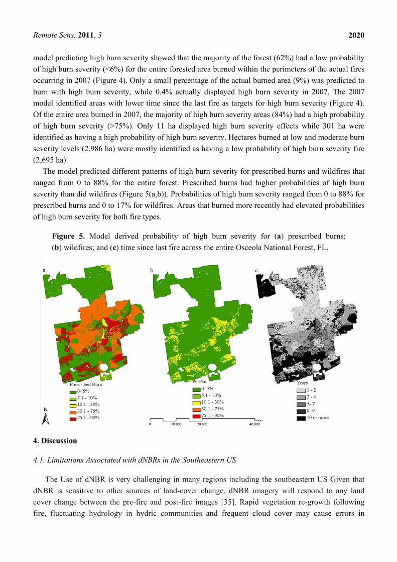
model predicting high burn severity showed that the majority of the forest (62%) had a low probability of high burn severity (<6%) for the entire forested area burned within the perimeters of the actual fires occurring in 2007 (Figure 4). Only a small percentage of the actual burned area (9%) was predicted to burn with high burn severity, while 0.4% actually displayed high burn severity in 2007. The 2007 model identified areas with lower time since the last fire as targets for high burn severity (Figure 4). Of the entire area burned in 2007, the majority of high burn severity areas (84%) had a high probability of high burn severity (>75%). Only 11 ha displayed high burn severity effects while 301 ha were identified as having a high probability of high burn severity. Hectares burned at low and moderate burn severity levels (2,986 ha) were mostly identified as having a low probability of high burn severity fire (2,695 ha).

The model predicted different patterns of high burn severity for prescribed burns and wildfires that ranged from 0 to 88% for the entire forest. Prescribed burns had higher probabilities of high burn severity than did wildfires (Figure 5(a,b)). Probabilities of high burn severity ranged from 0 to 88% for prescribed burns and 0 to 17% for wildfires. Areas that burned more recently had elevated probabilities of high burn severity for both fire types.

Figure 5. Model derived probability of high burn severity for (a) prescribed burns; (b) wildfires; and (c) time since last fire across the entire Osceola National Forest, FL.

4. Discussion

4.1. Limitations Associated with dNBRs in the Southeastern US

The Use of dNBR is very challenging in many regions including the southeastern US Given that dNBR is sensitive to other sources of land-cover change, dNBR imagery will respond to any land cover change between the pre-fire and post-fire images [35]. Rapid vegetation re-growth following fire, fluctuating hydrology in hydric communities and frequent cloud cover may cause errors in


2021

detecting burned severity [19]. Periodic variations in soil moisture and hydrology can influence the spectral reflectance values captured in dNBRs [36]. Standing water can also lead to the miss-classification of burned areas as unburned. The cyclical droughts experienced by the southeastern region of the US can cause a reduction in vegetation greenness that can mimic damage due to burn severity. Seasonal timing of fires and time lags between pre- and post-fire imagery also accounts for detected differences that are not associated with fire effects. When change in dNBR is due to natural phenological differences between pre- and post-fire images, there is a reduced distinction between burned and unburned areas and this could cause false positives for fire effects near or within burn perimeters. Nonetheless, dNBR has been shown to be a good measure of burn severity in the pine flatwoods of the south and can be used to identify the drivers of high fire severity.

4.2. Time and Severity Thresholds for Preventing High Burn Severity Effects

The probability of experiencing high burn severity, increasing and decreasing burn severity, and burning in subsequent fires has important implications for fire effects and the degree to which high severity fire is being mitigated. Based on the severity level of the first fire, fire type, and community type, we have the capacity to identify target time intervals between fires. On the Osceola National Forest, a time between fires of less than five years has been shown to have a mitigating effect on subsequent burn severity. After five years there is a marked increase in the probability of high burn severity (Figure 2(a)), of subsequent fires increasing in burn severity (Figure 2(b)), and fire risk. Previous studies conducted on the Osceola National Forest indicated that time between fires must be kept below three years to adequately reduce the occurrence of catastrophic wildfire [1]. Vegetation recovery following fire is expedient due to fast growing and re-sprouting species [37]. Lemon [38] used permanent plots on the Alapaha Experimental Range (Georgia) to monitor changes in vegetation following prescribed fire, and found that the maximum amount of litter is approached at five years’ post fire, while by eight years post fire vegetation returned to pre-burn status. Findings presented in Outcalt and Wade [2] and Lemon [38] support our results that identify target fire return intervals of less than five years to mitigate the effect of high burn severity in subsequent fires.

The relationship between fire occurrence and time interval between fires greater than six years implies that vegetation that has remained unburned for seven to 10 years may be less available to burn. This is likely due to higher fuel moisture contents and changes in species composition. Areas burned by wildfires also have a higher probability of subsequent high burn severity than areas first burned by prescribed fire and, hydric communities have a higher probability of high burn severity than mesic communities. Prescribed burns are performed under conditions that facilitate low severity fire effects. During prescribed burns, understory fuel in hydric communities is partially consumed with little consumption of the duff layer [2]. Therefore, hydric areas generally carry very heavy fuel volumes that become largely available during extended drought periods, making them capable of very large very intense wildfires [1].

Our results suggest that areas that have previously burned at high burn severity have a lower probability of decreasing in burn severity in subsequent fire. Although this result may seem counterintuitive, a study in New Mexico found that high burn severity areas were more likely to burn again at a high burn severity level in pinyon (Pinus L.) -juniper (Juniperus L.) woodlands [39].


2022

Although the vegetation types differ significantly, this phenomenon suggests that recovery time between fires where high burn severity occurred is long enough that the fuel structure and composition once again supports high severity fire. While recovering, these areas are less likely to be significantly altered by fire occurrence, simply because there is less fuel to be altered: In other words, remote sensing may underestimate burn severity in areas where fuels are limited as a result of high burn severity. Whether this phenomenon is a result of a positive relationship between fuels recovery and fire susceptibility, or the result of inherent limitations of using remote sensing analysis alone (i.e., without field validation) remains to be determined.

4.3. The Influence of Fire Frequency and Time since Last Fire on Severity

Fire frequency is one of the most important determinants for sustaining flatwoods ecosystems [40]. The relationship between fire frequency and the probability of high burn severity in prescribed burns and wildfires were not surprising; as frequencies increased the probability of high burn severity decreased (Figure 3). Post fire vegetation recovery to pre-fire biomass levels is rapid (1–4 years) in pine flatwoods forests [41-43]. Regular fire can reduce the amount of shrubby understory vegetation and promote grassy and herbaceous species that facilitate fire spread. Regular fire also reduces the growth of less-flammable broadleaf understory species and increases biodiversity [44]. Less frequent fire promotes aerial, surface, and ground fuel buildup, which likely facilitates high burn severity at least until significant composition change decreases flammability. The model developed here successfully captures the expected relationship between fire frequency and burn severity.

That the results suggest a negative relationship between time since last fire and the probability of high burn severity was surprising. We would expect the probability of high burn severity to increase with increased time since last fire [45], although the change in forest flammability associated with increased broadleaf abundance over time may help to explain this result. Previous studies of a single wildfire conducted in the Osceola National Forest found that as time between fire events increased from 1.5 to 3 years, post-fire tree mortality also increased [2]. Additional analysis of pine flatwoods elsewhere in the state showed similar trends [2]. A shift in dominant species from coniferous species to less flammable deciduous species could be responsible for the observed relationship between time since last fire and the probability of high burn severity. Deciduous litter is less aerated, and does not propagate fire spread and combustion as well as coniferous litter [44]. As deciduous encroachment increases over time, the probability of high burn severity may be decreased.

Expected changes in microclimate and fuel moisture content may also help explain why the model did not reflect the expected relationship between time since last fire and the probability of high burn severity. In the mesic-hydric pine flatwoods forests of the Osceola NF, fire initiation and spread are limited by the abundance of saw palmetto shrubs, which, although flammable, have higher moisture contents than most grassy or herbaceous species. High rates of decomposition result in minimal fine fuel accumulation on the forest floor. According to fuels management officers, lightning ignitions in the Osceola forest are far less frequent than those recorded in the nearby Appalachicola National Forest, where higher depth to the water table results in drier soils and a greater abundance of grassy and herbaceous fuels [46]. The negative relationship between time since last fire and the potential for high burn severity may be a result of higher fuel moisture contents, higher relative humidity, and lower


2023

temperatures where saw palmetto cover has had a longer time to recover from the previous fire. Where fire has more recently occurred, fine fuels from needle cast would contribute to the available fuel, temperatures and wind speed would be higher due to reduced canopy cover, and fire effects may be more severe when compared with long-unburned areas.

The negative relationship between time since last fire and the probability of high burn severity may also be due to a bias attributable to the influence of prescribed fires, which comprised 43% of the total fires used in the model. Suitable prescribed fire conditions are determined by time since last fire and fire frequency. Land managers may be willing to burn areas that were more recently burned under more extreme weather conditions due to lower fuel loads and lower potential for fire escape. Fire effects in these areas may then appear, at least temporarily, more severe than in areas that were burned under less extreme weather conditions. This may also be attributable to the fact that prescribed burns on the Osceola National Forest are primarily conducted in the winter, when canopies are less dense and fire severity at the ground level is more apparent in the imagery.

There is some support for these explanations: high pre-fire biomass may be the cause of the relationship between time since last fire and the probability of high burn severity. Previous studies have identified a relationship between burn severity level and pre-fire tree density [10,13]. Burn severity was highest in dense areas with high basal area and areas with high pre-fire litter and duff depths in the Coconino National Forest in Arizona [10]. These areas have the potential to both have and to indicate greater change between pre- and post-fire imagery [10]. Other authors have suggested that additional biases might exist. Using a relative version of dNBR, Miller and Thode [13] discovered a misclassification of areas with low vegetation due to the minimal detectable changes in a California forest. There was also a bias detected in classifying burn severity in multiple vegetation types using the same severity thresholds [13]. Allen and Sorbel [26] detected a similar bias in the low burn severity class for deciduous forest and tall shrubs in boreal forest and Tundra ecosystems in Alaska. In this study, severity values for deciduous forest were lower than their composite burn index (CBI).

4.4. Burn Severity in Relation to Fire Type, Community Type, and Forest Moisture

Overall, the probability of high burn severity in wildfires was less than what we would expect when compared to prescribed burns, which are commonly assumed to be lower in severity (Figure 5(a,b)). The low probability may have been caused by how wildfires were mapped or may indicate that active fire management on the Osceola is effectively suppressing high severity wildfire. Wildfire perimeters were mapped using Landsat imagery based on ocular estimates of where fires occurred. The perimeters were not always exact, resulting in unburned and low burn severity pixels occurring within the perimeter of a given wildfire. In contrast, prescribed burns tend to be more homogenous within their perimeters, as most are conducted during the winter season when fuels are uniformly dry. Also, most (70%) wildfires within this dataset were less than 10 ha in size. Wildfire size is determined by both suppression efforts and fuel availability, and if suppression is successful, fires are extinguished before fuels are extensively consumed, reducing the total area of high burn severity in wildfires. Successful fire suppression also implies that weather conditions may not have been conducive to promoting high burn severity effects. There were few wildfires (the Oak Fire of 1998, Friendly fire of 1999 Impassible Bay fire of 2004, and the Bugaboo fire of 2007) that were large (e.g., greater than 3,000 ha) in size and that


2024

required extensive suppression efforts. In this region, wildfires typically occur in the early spring, and the weather systems responsible for the lightning ignition may be accompanied by significant precipitation, increasing the patchiness of burns and ultimately reducing the overall continuity of burn severity. Our data shows that the majority of wildfires occurred in the spring, while most prescribed burns were conducted in the drier winter months. Fuel consumption may therefore be greater during the winter burns. Along with fire season, biases introduced by perimeter estimates and the higher proportion of smaller, less severe wildfires were likely causes for the low observed probability of experiencing high burn severity in wildfires.

Forest and community types were not significant predictors for subsequent high burn severity. We expected hydric communities to burn less severely in prescribed burns and potentially more severely during wildfires, when the high fuel loads could be dry enough to ignite during prolonged drought periods [2]. Within this dataset, there was no significant difference between fire effects in hydric and mesic forests. This lack of difference in fuel availability may have been due to suppression efforts or climatic factors. Suppression efforts may have been focused on preventing wildfires from entering areas of heavy fuel loads, climatic conditions during the burning of hydric areas may not have facilitated high burn severity effects. We also expected forest types to influence wildfire severity levels. The lack of significance may be due to the limited representation of non-flatwoods forest types in the Osceola National Forest (24%). Additional investigation into the relationships between forest age, structure, and severity patterns would increase our understanding of the importance of forest characteristics in affecting fire effects.

The spatial model identified areas where high severity prescribed burns and wildfires were expected to occur in 2007 based on fire frequency, fire type, and the amount of time since the last fire. Areas more recently burned exhibited a higher likelihood of high burn severity (Figure 5(a–c)). Most of the area impacted in 2007 was burned by prescribed fire and burned at moderate (21%) and low (78%) severity levels. Sections of the prescribed burns that actually displayed high burn severity had probabilities of high burn severity greater than 75% (Figure 4(a,b)). This suggests that the model adequately identified areas that had a high risk of high burn severity in a prescribed fire. The effectiveness of this model in predicting future burn severity should be further evaluated using remotely sensed burn severity data linked to ground-based evaluations. Given that the Osceola National Forest usually reaches its annual targets of 13,000 prescribed burn ha, there will be ample opportunity to validate this model here and in other flatwoods forests across the southern US.

5. Conclusions and Recommendations

Remote sensing techniques were successfully used to model nearly a decade’s worth of fires to determine high burn severity risk and important time thresholds for pine flatwoods management. The models identified areas that require attention in order to reduce the risk of high burn severity effects, especially for prescribed burns that are commonly assumed to exhibit low burn severity [47]. Our analysis indicates that time since last fire and fire frequency are major factors affecting the risk of high burn severity. A fire-free interval of less than five years is recommended to reduce the risk of high burn severity in pine flatwoods forests. Changes in vegetation and microclimate in response to less


2025

frequent fire may require more extreme weather conditions to burn [43], increasing the probability of high severity fires.

Areas that burned more recently had an elevated risk of high burn severity for both prescribed burns and wildfires. This result may be attributable to a bias in the detection of high severity effects in relation to pre-fire biomass, if areas that were recently burned are burned under more extreme weather prescriptions, or if vegetation recovery corresponds to a shift in flammability and microclimate that reduces burn severity. Further research addressing the relationship between pre-fire biomass, vegetation type, and dNBRs is necessary to determine if there is a bias occurring in the low severity class due to species composition, or a bias in the high severity class that is associated with high pre-fire biomass in pine flatwoods forests. In areas with short fire return intervals, it may also be useful to look at the effects of delayed mortality to identify if this would cause further error in detecting high burn severity effects. Directly following a fire, delayed mortality may cause a bias in the low burn severity class and, burn severity in subsequent fire may exhibit a bias in the high burn severity class due to the detection of fire effects from the previous fire.

The models created here can effectively identify time thresholds that facilitate increased risks of high burn severity and areas with an increased risk based on the history of fire. Additionally, the models are able to capture the relationship between fire frequency and high severity, and time between fires and increased risks of high burn severity. As fire frequency has been identified as an important indicator of ecosystem condition in flatwoods forest [40], these models can be used to inform prioritization and timing of fire use to maintain the pine flatwoods forests of the southern Coastal Plain.

Acknowledgements

This work was funded in part by the USDA National Needs Fellowship, and the Conserved Forest Ecosystems: Outreach and Research (CFEOR) cooperative at the University of Florida School of Forest Resources and Conservation. We thank Jason Drake at the US Forest Service Supervisors Office in Tallahassee, FL, USA, for providing data for this project, along with the personnel of the Osceola National Forest. We would also like to thank the Kobziar Fire Science Lab for their assistance.

References

1. Davis, L.S.; Cooper, R.W. How prescribed burning affects wildfire occurrence. J. For. 1963, 61, 915-917.

2. Outcalt, K.W.; Wade, D.D. Fuels management reduces tree mortality from wildfires in southeastern United States. South. J. Appl. For. 2004, 28, 28-34.

3. Main, M.B.; Richardson, L.W. Response of wildlife to prescribed fire in southwest Florida pine flatwoods. Wildl. Soc. Bull. 2002, 30, 213-133.

4. Heuberger, K.A.; Putz, F.E. Fire in the suburbs: Ecological impacts of prescribed fire in small remnants of longleaf pine sandhill. Restor. Ecol. 2003, 11, 72-81.


2026

5. Van Lear, D.H.; Carroll, W.D.; Kapeluck, P.R.; Johnson, R. History and restoration of the longleaf pine-grassland ecosystem: Implication for species at risk. For. Ecol. Manag. 2005, 211, 150-165.

6. Parr, C.L.; Andersen, A.N. Patch mosaic burning for biodiversity conservation: A critique of the pyro diversity paradigm. Conserv. Biol. 2006, 20, 1610-1619.

7. Wolcott, L.; O’Brien, J.J.; Mordecai, K. A survey of land managers on wildland hazardous fuels issues in Florida: A technical note. South. J. Appl. For. 2007, 31, 148-150.

8. Agee, J.K. Fire Ecology of Pacific Northwest Forest; Island Press: Washington, DC, USA, 1993; p. 417.

9. Hardy, C.C. Wildland fire hazard and risk: Problems, definitions, and context. For. Ecol. Manag. 2005, 211, 73-82.

10. Cocke, A.E.; Fule, P.Z.; Crouse, J.E. Comparison of burn severity assessment using difference Normalized Burn Ratio and ground data. Int. J. Wildl. Fire 2005, 14, 189-198.

11. Holden, Z.; Morgan, P.; Evans, J. A predictive model of burn severity based on 20-year satellite-infrared burn severity data in a large southwestern US wilderness area. For. Ecol. Manag. 2009, 258, 2399-2406.

12. Collins, B.M.; Miller, J.D.; Thode, A.E.; Kelly, M.; Wagtendonk, J.W.; Stephens, S. Interactions among wildland fires in a long-established sierra nevada natural fire area. Ecosystems 2009, 12, 114-128.

13. Miller, J.D.; Thode, A.E. Quantifying burn severity in a heterogeneous landscape with relative version of the delta Normalized Burn Ratio (dNBR). Remote Sens. Environ. 2007, 109, 66-80.

14. van Wagtendonk, J.W.; Root, R.R.; Key, C.H. Comparison of AVIRS and Landsat ETM+ detection capabilities for burn severity. Remote Sens. Environ. 2004, 92, 397-408.

15. Godwin, D.R. Burn severity in a central Florida sand pine scrub wilderness area. M.Sc. Thesis, University of Florida Press, Gainesville, FL, USA, 2008.

16. Hoy, E.E.; French, N.H.; Turetsky, M.R.; Trigg, S.N.; Kasischke, E.S. Evaluating the potential of landsat TM/ETM+ imagery for assessing fire severity in Alaska black spruce forest. Int. J. Wildl. Fire 2008, 17, 500-514.

17. White, J.D.; Ryan, K.C.; Key, C.C.; Runnig, S.W. Remote sensing of forest fire severity and vegetation recovery. Int. J. Wildl. Fire 1996, 6, 125-136.

18. French, N.H.F.; Kasischke, E.S.; Hall, R.J.; Murphy, K.A.; Verbyla, D.L.; Hoy, E.E.; Allen, J.L. Using Landsat data to assess fire and burn severity in the North American boreal forest region: An overview and summary of results. Int. J. Wildl. Fire 2008, 17, 443-462.

19. Picotte, J.J.; Robertson, K.M. Validation of remote sensing of burn severity in southeastern US ecosystems. Int. J. Wildl. Fire 2011, 20, 453-464.

20. Safford, H.D.; Schmidt, D.A.; Carson, C.H. Effects of fuel treatments on fire severity in an area of wildland-urban interface, Angora Fire, Lake Tahoe Basin, California. For. Ecol. Manag. 2009, 258, 773-787.

21. Kuenzi, A.M.; Fule, P.Z.; Sieg, C.H. Effects of fire severity and pre-fire stand treatment on plant community recovery after a large wildfire. For. Ecol. Manag. 2008, 255, 855-865.


2027

22. Oliveras, I.; Gracia, M.; Moré, G.; Retana, J. Factors influencing the patterns of fire severity in large wildland fire under extreme meteorological conditions in the Mediterranean basin. Int. J. Wildl. Fire 2009, 18, 755-764.

23. Eidenshink, J.; Schwind, B.; Brewer, K.; Zhu1, Z.; Quayle, B; Howard, S. A project for monitoring trends in burn severity. Fire Ecol. 2007, 3, 3-20.

24. Mitchener, L.J.; Parker, A.J. Climate, lightning, and wildfire in the national forests of the southeastern United States: 1989–1998. Phys. Geogr. 2005, 26, 147-162.

25. Earth Resources Observation and Science (EROS). Available online: http://glovis.usgs.gov/ distribution/downloadnotices.shtml (accessed on 7 January 2010).

26. Allen, J.L.; Sorbel, B. Assessing the differenced Normalized Burn Ratio’s ability to map burn severity in boreal forest and tundra ecosystems of Alaska’s national parks. Int. J. Wildl. Fire 2008, 17, 463-475.

27. Zhu, Z.; Key, C.H.; Ohlen, D.; Benson, N.C. Evaluate Sensitivities of Burn Severity Mapping Algorithms for Different Ecosystems and Fire Histories in the United States; Technical Report; Joint Fire Science Program: Boise, ID, USA, October 2006.

28. Key, C.H. Ecological and sampling constraints on defining landscape fire severity. Fire Ecol. 2006, 2, 34-59.

29. United States Geologic Service (USGS). Difference Normalized Burn Ratio. Available online: http://burnseverity.cr.usgs.gov/pdfs/LAv4_BR_ CheatSheet.pdf (accessed on 7 January 2010).

30. Alley, W.M. The palmer drought severity index: Limitations and assumptions. J. Clim. Appl. Meteorol. 1984, 23, 1100-1109.

31. Florida Natural Areas Inventory and Department of Natural Resources. Guide to the Natural Communities of Florida; Florida Natural Areas Inventory and Department of Natural Resources: Tallahassee, FL, USA, 1990.

32. Davis, J.H. General Map of Natural Vegetation in Florida. Agricultural Experimentations; Institute of Food and Agricultural Sciences, University of Florida: Gainesville, FL, USA, 1967.

33. Littell, R.C.; Milliken, G.A.; Stroup, W.W.; Wolfinger, R.D.; Schabenberger, O. SAS for Mixed Models, 2nd ed.; SAS Publishing: Caryn, NC, USA, 2006; p. 170.

34. SAS Institute Inc. SAS/STAT® 9.2 User’s Guide; SAS Institute Inc.: Cary, NC, USA, 2008. 35. Key, C.H. Remote Sensing Sensitivity to Fire Severity and Fire Recovery. In Proceedings of the

5th International Workshop on Remote Sensing and GIS Applications to Forest Fire Management: Fire Effects Assessment, Zaragoza, Spain, 16–18 June 2005.

36. Key, C.H.; Benson, N.C. Landscape Assessment: Ground Measure of Severity, the Composite Burn Index; and Remote Sensing of Severity, the Normalized Burn Ratio; Technical Report of the USDA Forest Service; Rocky Mountain Research Station: Ogden, UT, USA, 2006.

37. Lavoie, M.; Starr, G.; Mack, M.C.; Martin, T.A.; Gholz, H.L. Effects of a prescribed fire on understory vegetation, carbon pools, and soil nutrients in longleaf pine-slash pine forest in Florida. Natl. Areas J. 2010, 30, 82-94.

38. Lemon, P.C. Successional responses of herbs in the longleaf- slash pine forest after fire. Ecology 1949, 30, 135-145.

39. Holden, Z.A.; Morgan, P.; Hudak, A.T. Burn severity of areas reburned by wildfires in the Gila National Forest, New Mexico, USA. Fire Ecol. 2010, 6, 77-85.


2028

40. Mitchell, J.K.; Hiers, J.K.; O’Brien, J.J.; Jack, S.B.; Engstrom, R.T. Silviculture that sustains: The nexus between silviculture, frequent prescribed fire, and conservation of biodiversity in longleaf pine forests of the southeastern United States. Can. J. For. Resour. 2006, 36, 2724-2736.

41. Abrahamson, W.G. Species response to fire on the Florida Lake Wales Ridge. Am. J. Bot. 1984, 71, 35-43.

42. Abrahamson, W.G.; Abrahamson, C.R. Effects of fire on long unburned Florida uplands. J. Veg. Sci. 1996, 7, 565-574.

43. Maliakal, S.K.; Menges, E.S. Community composition and regeneration of Lake Wales Ridge wiregrass flatwoods in relation to time since last fire. J. Torrey Bot. Soc. 2000, 127, 125-138.

44 Moore, W.H.; Swindel, B.F.; Terry, S.W. Vegetative response to prescribed fire in a north Florida flatwoods forest. J. Range Manag. 1982, 35, 386-389.

45. DeBano, L.F.; Neary, D.G.; Ffolliott, P.F. Fire’s Effects on Ecosystems; Wiley: New York, NY, USA, 1998; pp. 333.

46. Kinghorn, S. USFS Osceola National Forest. Olustee, Florida, Personal Communication, 2010. 47. Van Wagtendonk, J.W.; Lutz, J.A. Fire regime attributes wildland fires in Yosemite National

Park, USA. Fire Ecol. 2007, 3, 34-52.

© 2011 by the authors; licensee MDPI, Basel, Switzerland. This article is an open access article distributed under the terms and conditions of the Creative Commons Attribution license (http://creativecommons.org/licenses/by/3.0/)

Modeling Relationships among 217 Fires Using Remote ...

Documents