Modeling Pulsar Trajectories Through a Galatic Potential ...

Union CollegeUnion | Digital Works

Honors Theses Student Work

6-2016

Modeling Pulsar Trajectories Through a GalaticPotential to Determine Birth LocationsBrent Shapiro-AlbertUnion College - Schenectady, NY

Follow this and additional works at: https://digitalworks.union.edu/theses

Part of the Astrophysics and Astronomy Commons

This Open Access is brought to you for free and open access by the Student Work at Union | Digital Works. It has been accepted for inclusion in HonorsTheses by an authorized administrator of Union | Digital Works. For more information, please contact [email protected].

Recommended CitationShapiro-Albert, Brent, "Modeling Pulsar Trajectories Through a Galatic Potential to Determine Birth Locations" (2016). HonorsTheses. 210.https://digitalworks.union.edu/theses/210

Modeling Pulsar Trajectories Through a

Galactic Potential to Determine Birth Locations

By

Brent Shapiro-Albert

∗ ∗ ∗ ∗ ∗ ∗ ∗ ∗ ∗

Submitted in partial fulfillment

of the requirements for

Honors in the Department of Physics and

Astronomy

UNION COLLEGE

March 2016

i

ABSTRACT

SHAPIRO-ALBERT, BRENT Modeling Pulsar Trajectories Through a Galactic Po-tential to Determine Birth Locations. Department of Physics and Astronomy,March 2016

ADVISOR: Gregory Hallenbeck

Neutron stars are the remnants of massive stars after their deaths in supernova ex-

plosions. Some neutron stars, called pulsars, are detected as periodic emitters of radio

waves at very precise intervals. Pulsars typically have higher velocities than their progen-

itor stellar population due to either kicks from supernova asymmetries or from remnant

velocities of compact binaries after they are disrupted by explosions. Their velocities

are large enough that pulsars will typically move large distances from their birth sites.

By determining a pulsar’s present day location and velocity, we project back to twice

the pulsar’s characteristic age to constrain the location of the progenitor star within the

uncertainty of the unknown line-of-sight velocity component.

Previous research by Hoogerwerf et al. (2001), Vlemmings et al. (2004), and Kirsten

et al. (2015) has traced back two pairs of objects, the pulsars B2020+28 and B2021+51,

and the pulsar and runaway star B1929 + 10 and ζ-Ophiuchi to determine their birth

locations and found each pair was associated in some way. Using a Python implemen-

tation with the Galpy package, we replicate the results from this previous research and

then project a new sample of 60 pulsars from the recent PSRPI survey back to determine

their birth locations. The potential birth regions are a sample of 36 OB star associations

selected from Tetzlaff et al. (2010). We also use this implementation to determine if there

are any birth associations between two pulsars in our sample within the same region. We

find that we can successfully model a pulsar’s trajectory and determine a likely birth OB

region for a pulsar with our model.

ii

Contents

1 Introduction 1

1.1 Velocities and Origin of Pulsars . . . . . . . . . . . . . . . . . . . . . . . 4

2 Methods 7

2.1 Data and Estimates . . . . . . . . . . . . . . . . . . . . . . . . . . . . . . 7

2.1.1 Duration of Trajectories . . . . . . . . . . . . . . . . . . . . . . . 10

2.1.2 The Radial Velocity Distribution . . . . . . . . . . . . . . . . . . 12

2.1.3 Determining Pulsar Birth Regions . . . . . . . . . . . . . . . . . . 15

2.2 Computational Methods . . . . . . . . . . . . . . . . . . . . . . . . . . . 18

2.2.1 Implementation . . . . . . . . . . . . . . . . . . . . . . . . . . . . 18

2.2.2 Using Galpy to Simulate Trajectories . . . . . . . . . . . . . . . . 22

2.2.3 Initial Pair Tests . . . . . . . . . . . . . . . . . . . . . . . . . . . 23

3 Initial Results 29

3.1 ζ Ophiuchi and B1929+10 . . . . . . . . . . . . . . . . . . . . . . . . . . 29

3.2 B2020+28 and B2021+51 . . . . . . . . . . . . . . . . . . . . . . . . . . 32

4 Results of PSRPI Trajectories 35

4.1 Pulsar Pairs from the Same OB Region: J0102+6537 and J0357+5236 . . 35

4.2 Pulsar Pairs with No OB Region Matches . . . . . . . . . . . . . . . . . 45

4.3 Pulsar Birth OB Regions: J0055+5117 and Cas OB2 . . . . . . . . . . . 46

5 Conclusions 50

6 Appendix A 54

iii

1 Introduction

When a massive star dies in a supernova explosion, the inner core can collapse back

into a white dwarf, a hot, dense star which is supported by electron degeneracy pressure.

However, when the cores of these stars are very massive, the gravitational pressure over-

comes the electron degeneracy pressure and the white dwarf collapses further. In this

scenario, electrons and protons combine to form neutrons. These neutrons are packed

so densely that there is no space between them. These extremely compact objects are

called neutron stars and are supported by neutron degeneracy pressure (Hoyle et al.,

1964). Some of these neutron stars rotate very rapidly and emit radio waves along their

magnetic poles. Neutron stars that emit these radio waves are called pulsars, since as

these neutron stars rotate, the radio waves they emit pass through our line of sight with

a very precise period, creating a radio pulse.

Pulsars can be used as a laboratory to study extreme physics that we cannot replicate

on Earth. We can study extreme magnetic environments on the order of 108 to 1012

G. Neutron stars are also incredibly dense which allows us to perform tests of General

Relativity (“GR”) and identify post-Keplerian corrections (Lorimer, 2008) to their orbits.

In addition to these extreme environmental tests, pulsar binary pairs have been shown

to be an indirect source of gravitational waves (Hulse & Taylor, 1975). It has also been

theorized that we can directly detect these waves by long-term timing of a large array of

pulsars (Jenet et al., 2009). If we have measurements of the motions of the pulsar we can

also model its trajectory to try to find an associated supernova remnant (SNR) and learn

more about pulsar birth supernovae (Dewey & Cordes, 1987, Vlemmings et al., 2004).

The first binary pulsar discovered was B1913 + 16, also known as the Hulse-Taylor

binary. Careful study of this binary pulsar showed that the orbital period of the pulsar

1

and its invisible companion steadily decreased over time. Since GR predicts that the

binary pair will radiate energy as gravitational waves, the system will lose energy over

time and the orbital period will decrease as a result. The observed decrease in orbital

period were found to match the predictions of GR (Hulse & Taylor, 1975). The amount

of energy lost by the system is consistent with the amount of energy predicted to be

lost due to gravitational wave emission, thus showing indirect evidence for gravitational

waves (Hulse & Taylor, 1975).

Additionally, GR predicts orbits for close binary pairs which differ from the Keplerian

orbits of Newtonian gravity. In a two-pulsar binary system, the magnetospheres can in-

fluence the radio pulses we see from each pulsar which allow us to measure the relativistic

spin-orbital coupling (Graham-Smith & McLaughlin, 2005) which can also constrain pre-

dictions made by GR. Some binary orbits require corrections from GR, which come from

equations utilizing “post-Keplerian” (PK) parameters (Lorimer, 2008). Depending on

the observing conditions there are 19 different parameters that can be measured leading

to 15 different tests of GR (Damour & Taylor, 1992). Since 1974 many pulsar binary

tests of GR have occurred including further timing of B1913 + 16. This has shown that

the decrease in orbital period of B1913 + 16 and its invisible companion agrees with the

expected emission of gravitational waves, according to GR, to within 0.2% up to present

day (Weisberg & Taylor, 2005). Other similar tests have been made in good agreement

with the GR predictions (Jacoby et al., 2006, Stairs et al., 2002) and as instrumentation

improves it is likely that more binary pulsars will be found and the number of GR tests

will grow.

Pulsar periods can be measured using a baseline of a few months to an accuracy of

around 10−7 s or better (Jenet et al., 2009). Some pulsars, such as B1937+21, have been

timed to an accuracy of 10−13 s using a longer baseline of a few years (Davis et al., 1985).

2

The precision timing of pulsars can also be used to directly detect gravitational waves due

to perturbations in the pulse periods from these waves. Theory predicts that by observing

an ensemble of high-precision radio pulsars we will see fluctuations in the pulse arrival

times from pulsars at nHz frequencies due to these gravitational waves. One group is the

North American Nanohertz Observatory for Gravitational Waves (NANOGrav), which is

a consortium of institutes and researchers using pulsar timing arrays which utilize pulsars

as both a source of radio emission and a clock to time the radio pulses (Jenet et al., 2009).

NANOGrav is also part of a global consortium along with the European Pulsar Timing

Array (EPTA) and the Parkes Pulsar Timing Array (PPTA) which together form the

International Pulsar Timing Array (IPTA). While the timing of many pulsars is better

than 100 ns (Jenet et al., 2009), variation in the pulse arrival times from the Interstellar

Medium (ISM), the pulsar itself, and the measurement process must be accounted for

(Lam et al., 2015). Reducing the intrinsic pulse “jitter” and the observational noise, from

factors such as the ISM, is a key step in direct detection of gravitational waves.

While pulsars have very strong magnetic fields, a particular class of pulsars called

magnetars have magnetic fields between 1014-1015 G. Magnetars are thus expected to

be born in highly energetic supernovae with millisecond periods at birth (Duncan &

Thompson, 1992). An alternative theory for magnetar birth is that the progenitor stars

already have highly magnetic cores and the neutron stars formed during supernovae obtain

large magnetic fields through magnetic flux conservation (Ferrario & Wickramasinghe,

2008). Current models underestimate the number of magnetars found in surveys thus far

which poses a magnetar birthrate problem (Turolla et al., 2015). This suggests that we

are not accounting for all of the possible ways a neutron star may acquire a magnetic

field this strong. Magnetars are also observed to emit large flares in the X-ray. One

explanation for these flares is sudden reconfigurations in the magnetosphere (Turolla et

3

al., 2015).

Pulsars with planets such as B1257 + 12 allow us to study the effects of extreme

magnetic fields on planetary orbits and also allow us to constrain the birth parameters

necessary to have a planet. B1257 + 12 was found to have a small magnetic field at birth,

which suggests this is a necessary condition for a pulsar to have a planet (Cordes, 1993,

Kohler, 2015).

1.1 Velocities and Origin of Pulsars

Pulsars are observed to have very large velocities perpendicular to our line of sight, or

transverse velocity (V⊥), with many moving across the sky at speeds of a few hundred

km s−1 (Gott et al., 1970). The pulsar B1508 + 55 has an observed transverse velocity of

1083+103−90 km s−1 (Chatterjee et al., 2005), which is larger than the escape velocity of the

galaxy. Examining the birth scenarios of pulsars gives insight into the origin of the large

V⊥ that we observe. If we are able to determine the past trajectory of a pulsar in some

cases it may be possible to determine a likely birth site or SNR. One theory behind these

large V⊥ is asymmetric supernova “birth kicks” that would impart V⊥ of ∼ 100 km s−1.

(Chatterjee et al., 2005, Dewey & Cordes, 1987). However, in most models, this “kick”

is not enough to give many pulsars the observed V⊥, producing mostly V⊥ ≤ 30 km s−1

(Dewey & Cordes, 1987). In the case of B1508 + 55, a single asymmetric supernova was

unable to account for the large V⊥. Other theories, such as neutrino driven kicks within

the supernova due to large magnetic fields on the order of 1016 G (Lai et al., 2001) or

a disrupted binary system (Iben & Tutukov, 1996) were also found to be inadequate to

produce a V⊥ > 1000 km s−1. Some combination of these mechanisms is concluded to be

the most likely scenario, although no definite conclusions are drawn on how B1508 + 55

4

obtains its large V⊥. We can further study the mechanisms behind these large V⊥ by

tracing back the pulsar’s trajectory to determine where its progenitor star was located

and examine possible pulsar birth scenarios.

One recent pulsar survey is Pulsar Parallax (PSRPI) which observed the parallax (π)

and proper motions (µ), the angular motion of a star across sky, of 60 pulsars using the

Very Large Baseline Array (VLBA). All pulsars in this survey are within 4 kpc of the sun

and all measurements of µ and π had uncertainties less than 10%. The PSRPI survey

has four goals: accurately measuring the distances to pulsars, improving Galactic elec-

tron density distribution models, associating pulsars with SNRs, and improving the ties

between the International Celestial Reference Frame (ICRF), optical, and solar system

barycenter frames (Deller et al., 2011). The results from PSRPI are thus essential in try-

ing to map the galactic distribution of pulsars. Improving the distances and luminosities

of these pulsars allow us to determine what the previous errors in distance and luminos-

ity measurements may be. By correcting these errors, we can correct the pulsar distance

and pulsar luminosity functions, which describe the galactic distribution of pulsars. To

associate pulsars with SNRs, we need to simulate their trajectories which utilize π and

µ measurements (Deller et al., 2011). We can also estimate the distribution of pulsars

across the galaxy, which allows us to examine the birth scenarios of these pulsars and

better model large star supernovae. Since it is difficult to find pulsars because they are

very faint, we know little about pulsars outside of the local population.

Although the large progenitor stars of pulsars generally have velocities of just a few

10’s of km s−1 we measure V⊥ in many pulsars to be a few 100’s of km s−1. One motivation

for determining birth locations of pulsars is to determine how pulsars obtain these much

larger V⊥. One prominent theory is that asymmetric SNe impart a birth “kick” to the

neutron star that is formed at its core which gives the pulsar its large velocity (Dewey

5

& Cordes, 1987). If we can associate a pulsar with an SNR, then we can determine if

the SNe is what imparted the large velocity to the pulsar, or if other factors may have

contributed to it. However it is difficult to associate a pulsar with a particular SNR for

a variety of reasons.

The focus of this work is to determine the birth locations of 60 pulsars from the

PSRPI survey. In Chapter 2 we will discuss the problem posed by radial velocities (Vr)

and our estimated distributions of Vr for this distribution of pulsars (Hobbs et al., 2005).

We will also discuss our pulsar trajectory model used to determine the birth locations of

the PSRPI pulsars in Chapter 2. In Chapter 3 we will use our model to reproduce the

results of Hoogerwerf et al. (2001), Vlemmings et al. (2004), and Kirsten et al. (2015)

who determined the birth locations of two different pulsar pairs found to have a common

origin, the runaway star ζ-Ophiuchi and pulsar B1929+10 and the pulsar pair B2020+28

and B2021 + 51. We will then present the results of our model for all the PSRPI pulsars

in Chapter 4.

6

2 Methods

2.1 Data and Estimates

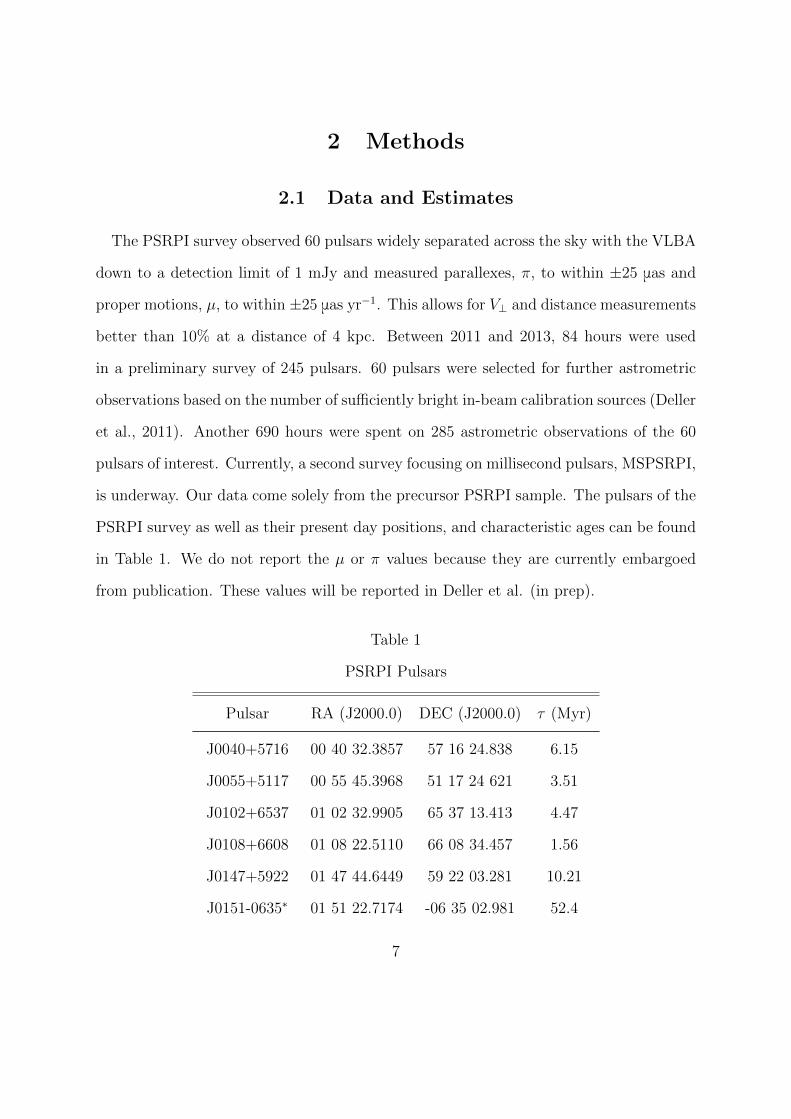
The PSRPI survey observed 60 pulsars widely separated across the sky with the VLBA

down to a detection limit of 1 mJy and measured parallexes, π, to within ±25 μas and

proper motions, µ, to within ±25 μas yr−1. This allows for V⊥ and distance measurements

better than 10% at a distance of 4 kpc. Between 2011 and 2013, 84 hours were used

in a preliminary survey of 245 pulsars. 60 pulsars were selected for further astrometric

observations based on the number of sufficiently bright in-beam calibration sources (Deller

et al., 2011). Another 690 hours were spent on 285 astrometric observations of the 60

pulsars of interest. Currently, a second survey focusing on millisecond pulsars, MSPSRPI,

is underway. Our data come solely from the precursor PSRPI sample. The pulsars of the

PSRPI survey as well as their present day positions, and characteristic ages can be found

in Table 1. We do not report the µ or π values because they are currently embargoed

from publication. These values will be reported in Deller et al. (in prep).

Table 1

PSRPI Pulsars

Pulsar RA (J2000.0) DEC (J2000.0) τ (Myr)

J0040+5716 00 40 32.3857 57 16 24.838 6.15

J0055+5117 00 55 45.3968 51 17 24 621 3.51

J0102+6537 01 02 32.9905 65 37 13.413 4.47

J0108+6608 01 08 22.5110 66 08 34.457 1.56

J0147+5922 01 47 44.6449 59 22 03.281 10.21

J0151-0635∗ 01 51 22.7174 -06 35 02.981 52.4

7

Pulsar RA (J2000.0) DEC (J2000.0) τ (Myr)

J0152-1637 01 52 10.8539 -16 37 53.597 10.2

J0157+6212 01 57 49.9431 62 12 26.616 0.197

J0323+3944∗ 03 23 26.6594 39 44 52.435 75.6

J0332+5434∗∗ 03 32 59.4071 54 34 43.341 5.53

J0335+4555∗ 03 35 16.6420 45 55 53.450 580

J0357+5236 03 57 44.8392 52 36 57.502 6.55

J0406+6138 04 06 30.0793 61 38 41.384 1.69

J0601-0527† 06 01 58.9755 -05 27 50.847 4.82

J0614+2229 06 14 17.0055 22 29 56.849 0.0893

J0629+2415 06 29 05.7271 24 15 41.549 3.78

J0729-1836 07 29 32.3378 -18 36 42.255 0.426

J0823+0159∗ 08 23 09.7652 01 59 12.466 131

J0826+2637 08 26 51.5024 26 37 21.385 4.92

J1022+1001∗ 10 22 57.9963 10 01 52.760 60.2

J1136+1551 11 36 03.1234 15 51 13.893 5.04

J1257-1027 12 57 04.7626 -10 27 05.555 27.0

J1321+8323 13 21 45.6636 83 23 39.396 18.7

J1532+2745 15 32 10.3643 27 45 49.606 22.9

J1543-0620 15 43 30.1390 -06 20 45.323 12.8

J1607-0032 16 07 12.0619 -00 32 41.500 21.8

J1623-0908 16 23 17.6598 -09 08 48.853 7.84

J1645-0317 16 45 02.0408 -03 17 57.834 3.45

J1650-1654∗∗ 16 50 27.1700 -16 54 42.269 8.66

8

Pulsar RA (J2000.0) DEC (J2000.0) τ (Myr)

J1703-1846 17 03 51.0913 -18 46 14.872 7.36

J1735-0724 17 35 04.9730 -07 24 52.155 5.47

J1741-0840 17 41 22.5628 -08 40 31.717 14.2

J1754+5201 17 54 22.9072 52 01 12.241 24.2

J1820-0427 18 20 52.5935 -04 27 37.728 1.5

J1833-0338 18 33 41.8955 -03 39 04.270 0.262

J1840+5640 18 40 44.5407 56 40 54.877 17.5

J1901-0906 19 01 53.0091 -09 06 11.133 17.2

J1912+2104 19 12 43.3396 21 04 33.930 3.48

J1913+1400 19 13 24.3529 14 00 52.564 10.3

J1917+1353 19 17 39.7864 13 53 57.073 0.428

J1919+0021 19 19 50.6711 00 21 39.721 2.63

J1937+2544 19 37 01.2550 25 44 13.446 4.95

J2006-0807∗ 20 06 16.3653 -08 07 02.159 200

J2010-1323∗ 20 10 45.9209 -13 23 56.081 1.72e4

J2046-0421 20 46 00.1723 -04 21 26.254 16.7

J2046+1540∗ 20 46 39.3378 15 40 33.557 98.9

J2113+2754 21 13 04.3524 27 54 01.207 7.27

J2113+4644 21 13 24.3287 46 44 08.836 22.5

J2145-0750∗ 21 45 50.4591 -07 50 18.513 8.54e3

J2149+6329 21 49 58.7018 63 29 44.271 35.8

J2150+5247† 21 50 37.7493 52 47 49.559 0.521

J2212+2933∗ 22 12 23.3448 29 33 05.418 32.1

9

Pulsar RA (J2000.0) DEC (J2000.0) τ (Myr)

J2225+6535∗∗ 22 25 52.8448 65 35 36.275 1.12

J2248-0101 22 48 26.8864 -01 01 48.071 11.5

J2305+3100 23 05 58.3214 31 00 01.291 8.63

J2317+1439 23 17 09.2364 14 39 31.261 2.26e4

J2317+2149∗ 23 17 57.8414 21 49 48.019 21.9

J2325+6316 23 25 13.3204 63 16 52.362 8.05

J2346-0609 23 46 50.4960 -06 09 59.884 13.7

J2354+6155 23 54 04.7808 61 55 46.840 0.92

Table 1: The sample of 60 pulsars from PSRPI. We have included the coordinates in RAand Dec (J2000.0) from the PSRPI project web page. It also includes the characteristicages of each pulsar in Myr from the PSRCAT database. A “∗” denotes that the pulsaris too old to be accurately traced back. A “∗∗” denotes that data were not received inthe final results. A “†” denotes an unresolved issue that led to an inability to accuratelytrace the pulsar back in time.

2.1.1 Duration of Trajectories

One estimate of a pulsar’s age is its characteristic age, τ . We will reproduce the common

derivation of τ here. This is done by assuming that any change in the pulsar’s magnetic

field strength and angle of inclination is negligible. We also assume that the pulsar’s

current period is much longer than its birth period. We will represent the present day

period by P and the initial period be P0. We know from observations that the periods

of pulsars change (Richards & Comella, 1969). By definition, the change rate of change

in the period is

10

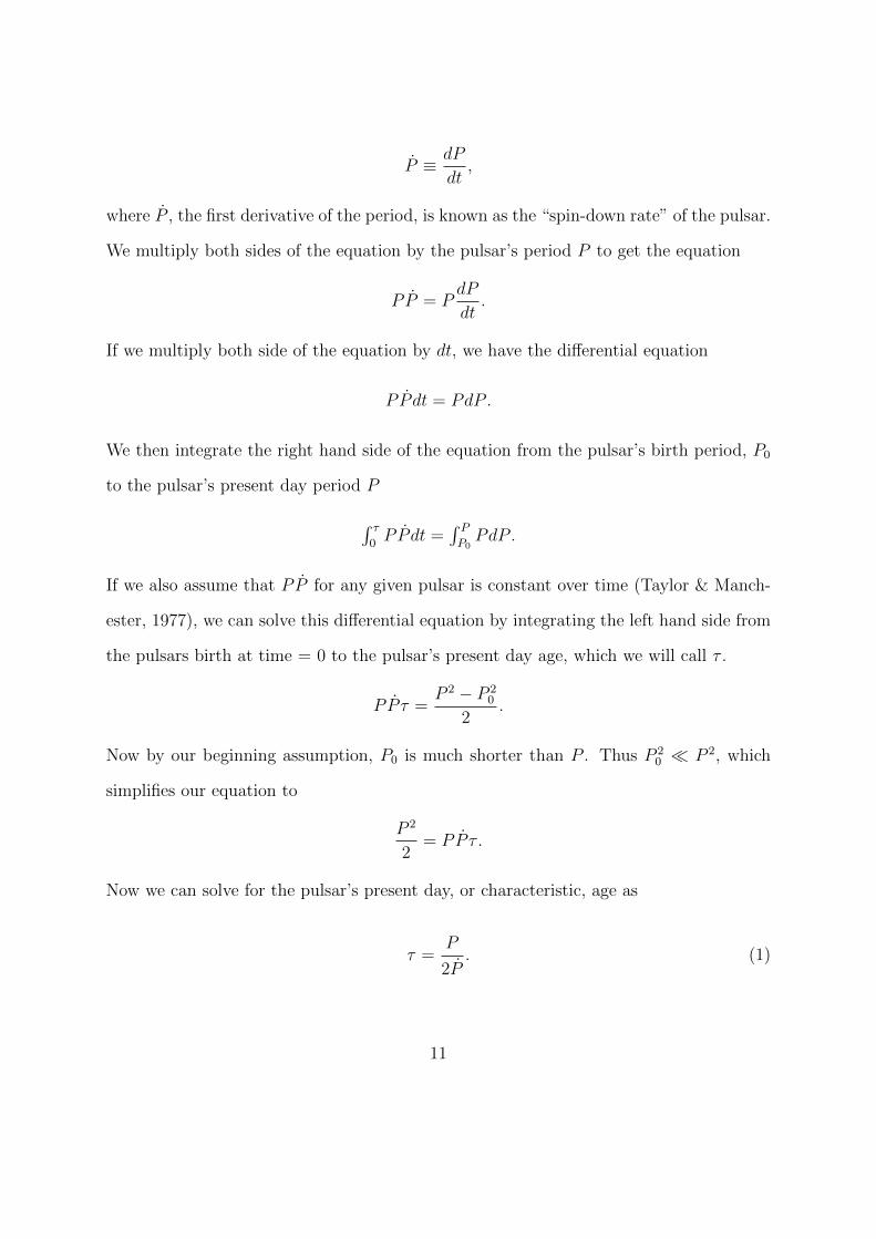
P ≡ dP

dt,

where P , the first derivative of the period, is known as the “spin-down rate” of the pulsar.

We multiply both sides of the equation by the pulsar’s period P to get the equation

PP = PdP

dt.

If we multiply both side of the equation by dt, we have the differential equation

PPdt = PdP .

We then integrate the right hand side of the equation from the pulsar’s birth period, P0

to the pulsar’s present day period P

∫ τ0PPdt =

∫ PP0PdP .

If we also assume that PP for any given pulsar is constant over time (Taylor & Manch-

ester, 1977), we can solve this differential equation by integrating the left hand side from

the pulsars birth at time = 0 to the pulsar’s present day age, which we will call τ .

PP τ =P 2 − P 2

0

2.

Now by our beginning assumption, P0 is much shorter than P . Thus P 20 � P 2, which

simplifies our equation to

P 2

2= PP τ .

Now we can solve for the pulsar’s present day, or characteristic, age as

τ =P

2P. (1)

11

However, since τ is known to be imprecise and generally overestimate the pulsar’s age

(Taylor & Manchester, 1977), we will trace each pulsar’s trajectory back to a maximum

of 2τ .

Once pulsars have τ more than a few 10’s of Myr old, other interactions that the

pulsar may have had can change the values of µ and π that a pulsar may have had at

birth. We thus limit our study to younger pulsars with τ . 30 Myr. However there

is a chance that these young pulsars have been “recycled.” These objects usually are

older pulsars that have had their pulse periods sped-up again by accreting matter from a

companion star, which increases their angular momentum (Tauris, 1994). These recycled

pulsars often have millisecond periods which would lead to shorter inferred τ . Recycled

pulsars will also have different values of µ and π than may have been observed at birth

and so cannot be traced back (Bisnovatyi-Kogan, 2006). The PSRPI survey does not

include any millisecond pulsars in order to try to avoid projecting back the trajectories

of recycled pulsars. We cannot be sure that the pulsars in our sample were never part of

a binary system. However since we know that none have millisecond periods, we know

that none have been in a binary for at least the duration of their characteristic age. Thus

we can still trace a pulsar back to its binary origin if not its actual birth OB region.

2.1.2 The Radial Velocity Distribution

We have now five of the six values needed to trace the trajectories of our pulsars, the

pulsar’s position in RA and Dec, µ (in RA and Dec), and π, from the PSRPI survey. The

last value necessary to simulate the pulsar’s trajectory is Vr, the velocity along the line-

of-sight, which we cannot measure. Since pulsars are not visible at optical wavelengths,

we cannot determine Vr from the Doppler shift of known spectral lines. Instead we

approximate Vr based on V⊥ measurements (Hobbs et al., 2005) to derive a Gaussian

12

probability density function (PDF) of possible values of Vr for any pulsar. The use of

a Gaussian Vr Distribution is standard when simulating the trajectories of pulsars to

determine their birth regions (Hoogerwerf et al., 2001, Kirsten et al., 2015). We use a

previous analysis of 233 pulsars and their proper motions from Hobbs et al. (2005) to

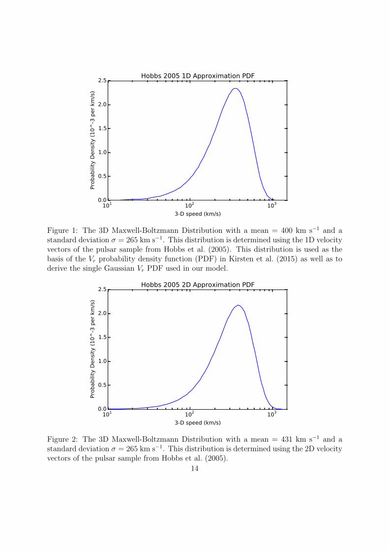
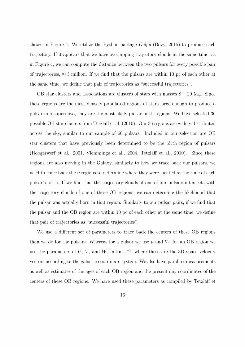
estimate Vr. This study derived a Maxwell-Boltzmann Distribution of three dimensional

(3D) space velocities for pulsars.

While we cannot directly measure the 3D space velocity of a pulsar, we can generally

measure the one or two dimensional space velocity. Since this observed data is consistent

with an isotropic velocity vector, we can then obtain a 3D space velocity distribution

from the 1D and 2D velocity measurements using a deconvolution technique (Hobbs

et al., 2005). Hobbs et al. (2005) obtains two, one-sided 3D Vr Maxwell-Boltzmann

Distributions, one from the 1D velocities and the other from the 2D velocities, with peaks

at 400 km s−1 and 431 km s−1 respectively. These distribution are shown in Figures 1

and 2 and estimate the distribution of the unobservable Vr component.

However, since the pulsars can be moving towards us (Vr < 0 ) or away from us

(Vr > 0), the distribution must include negative Vr values (Hoogerwerf et al., 2001,

Vlemmings et al., 2004, Kirsten et al., 2015). Since Hobbs et al. (2005) determined

a Maxwell-Boltzmann distribution which contains only positive velocities, we translate

their distribution to determine a standard deviation (σ) of this distribution and use it as

the σ for a single Gaussian Distribution centered on 0 km s−1. We determined σ to be 578

km s−1. This allows us to make a direct comparison of our results with past results and

minimize the amount of uncertainty between the different models. We use the Gaussian

distribution in Figure 3 in our Monte Carlo simulations of the pulsar trajectories.

13

101 102 103

3-D speed (km/s)

0.0

0.5

1.0

1.5

2.0

2.5

Pro

babili

ty D

ensi

ty (

10^

-3 p

er

km/s

)

Hobbs 2005 1D Approximation PDF

Figure 1: The 3D Maxwell-Boltzmann Distribution with a mean = 400 km s−1 and astandard deviation σ = 265 km s−1. This distribution is determined using the 1D velocityvectors of the pulsar sample from Hobbs et al. (2005). This distribution is used as thebasis of the Vr probability density function (PDF) in Kirsten et al. (2015) as well as toderive the single Gaussian Vr PDF used in our model.

101 102 103

3-D speed (km/s)

0.0

0.5

1.0

1.5

2.0

2.5

Pro

babili

ty D

ensi

ty (

10^

-3 p

er

km/s

)

Hobbs 2005 2D Approximation PDF

Figure 2: The 3D Maxwell-Boltzmann Distribution with a mean = 431 km s−1 and astandard deviation σ = 265 km s−1. This distribution is determined using the 2D velocityvectors of the pulsar sample from Hobbs et al. (2005).

14

2000 1500 1000 500 0 500 1000 1500 2000

Radial Velocity (km/s)

0.0

0.2

0.4

0.6

0.8

1.0

Pro

babili

ty D

ensi

ty (

10^

-3 p

er

km/s

)

Radial Velocity PDF

Figure 3: The Gaussian Vr PDF that we have derived from the PDF shown in Table 1.This distribution is centered an 0 km s−1 and has σ = 578 km s−1. This distributionallows us to account for negative values of Vr.

2.1.3 Determining Pulsar Birth Regions

Of the initial 60 pulsars only 46 have estimated ages below the upper limit τ . 30

Myr to avoid recycled pulsars. Additionally, we find 2 pulsars whose trajectories result

in unrealistic trajectory clouds showing birth regions 100’s to 1000’s of kpc away from

the Milky Way. The reason for this has yet to be resolved at the time of this writing.

We therefore use a sample size of 44 pulsars for the remainder of this work. The pulsars

that we do not use in our sample are denoted with a ∗, ∗∗, or † in Table 1. To determine

the birth locations of these 44 pulsars we simulate their trajectories through a galactic

potential. We do this using a Monte Carlo simulation, sampling each parameter, π, µ, and

Vr, from Gaussian Probability Density Functions (PDFs) and generating 1750 potential

orbits for each pulsar which form a 3D trajectory cloud. An example pair of clouds is

15

shown in Figure 4. We utilize the Python package Galpy (Bovy, 2015) to produce each

trajectory. If it appears that we have overlapping trajectory clouds at the same time, as

in Figure 4, we can compute the distance between the two pulsars for every possible pair

of trajectories, ≈ 3 million. If we find that the pulsars are within 10 pc of each other at

the same time, we define that pair of trajectories as “successful trajectories”.

OB star clusters and associations are clusters of stars with masses 8 − 20 M�. Since

these regions are the most densely populated regions of stars large enough to produce a

pulsar in a supernova, they are the most likely pulsar birth regions. We have selected 36

possible OB star clusters from Tetzlaff et al. (2010). Our 36 regions are widely distributed

across the sky, similar to our sample of 60 pulsars. Included in our selection are OB

star clusters that have previously been determined to be the birth region of pulsars

(Hoogerwerf et al., 2001, Vlemmings et al., 2004, Tetzlaff et al., 2010). Since these

regions are also moving in the Galaxy, similarly to how we trace back our pulsars, we

need to trace back these regions to determine where they were located at the time of each

pulsar’s birth. If we find that the trajectory clouds of one of our pulsars intersects with

the trajectory clouds of one of these OB regions, we can determine the likelihood that

the pulsar was actually born in that region. Similarly to our pulsar pairs, if we find that

the pulsar and the OB region are within 10 pc of each other at the same time, we define

that pair of trajectories as “successful trajectories”.

We use a different set of parameters to trace back the centers of these OB regions

than we do for the pulsars. Whereas for a pulsar we use µ and Vr, for an OB region we

use the parameters of U , V , and W , in km s−1, where these are the 3D space velocity

vectors according to the galactic coordinate system. We also have parallax measurements

as well as estimates of the ages of each OB region and the present day coordinates of the

centers of these OB regions. We have used these parameters as compiled by Tetzlaff et

16

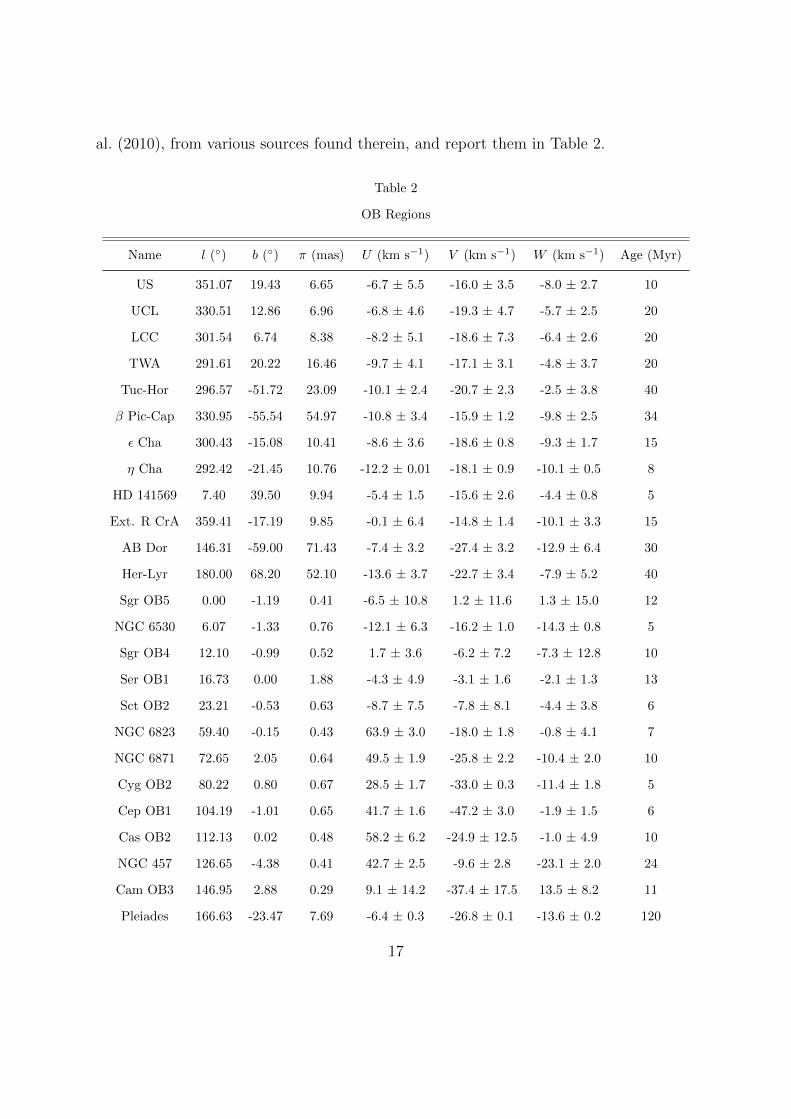
al. (2010), from various sources found therein, and report them in Table 2.

Table 2

OB Regions

Name l (◦) b (◦) π (mas) U (km s−1) V (km s−1) W (km s−1) Age (Myr)

US 351.07 19.43 6.65 -6.7 ± 5.5 -16.0 ± 3.5 -8.0 ± 2.7 10

UCL 330.51 12.86 6.96 -6.8 ± 4.6 -19.3 ± 4.7 -5.7 ± 2.5 20

LCC 301.54 6.74 8.38 -8.2 ± 5.1 -18.6 ± 7.3 -6.4 ± 2.6 20

TWA 291.61 20.22 16.46 -9.7 ± 4.1 -17.1 ± 3.1 -4.8 ± 3.7 20

Tuc-Hor 296.57 -51.72 23.09 -10.1 ± 2.4 -20.7 ± 2.3 -2.5 ± 3.8 40

β Pic-Cap 330.95 -55.54 54.97 -10.8 ± 3.4 -15.9 ± 1.2 -9.8 ± 2.5 34

ε Cha 300.43 -15.08 10.41 -8.6 ± 3.6 -18.6 ± 0.8 -9.3 ± 1.7 15

η Cha 292.42 -21.45 10.76 -12.2 ± 0.01 -18.1 ± 0.9 -10.1 ± 0.5 8

HD 141569 7.40 39.50 9.94 -5.4 ± 1.5 -15.6 ± 2.6 -4.4 ± 0.8 5

Ext. R CrA 359.41 -17.19 9.85 -0.1 ± 6.4 -14.8 ± 1.4 -10.1 ± 3.3 15

AB Dor 146.31 -59.00 71.43 -7.4 ± 3.2 -27.4 ± 3.2 -12.9 ± 6.4 30

Her-Lyr 180.00 68.20 52.10 -13.6 ± 3.7 -22.7 ± 3.4 -7.9 ± 5.2 40

Sgr OB5 0.00 -1.19 0.41 -6.5 ± 10.8 1.2 ± 11.6 1.3 ± 15.0 12

NGC 6530 6.07 -1.33 0.76 -12.1 ± 6.3 -16.2 ± 1.0 -14.3 ± 0.8 5

Sgr OB4 12.10 -0.99 0.52 1.7 ± 3.6 -6.2 ± 7.2 -7.3 ± 12.8 10

Ser OB1 16.73 0.00 1.88 -4.3 ± 4.9 -3.1 ± 1.6 -2.1 ± 1.3 13

Sct OB2 23.21 -0.53 0.63 -8.7 ± 7.5 -7.8 ± 8.1 -4.4 ± 3.8 6

NGC 6823 59.40 -0.15 0.43 63.9 ± 3.0 -18.0 ± 1.8 -0.8 ± 4.1 7

NGC 6871 72.65 2.05 0.64 49.5 ± 1.9 -25.8 ± 2.2 -10.4 ± 2.0 10

Cyg OB2 80.22 0.80 0.67 28.5 ± 1.7 -33.0 ± 0.3 -11.4 ± 1.8 5

Cep OB1 104.19 -1.01 0.65 41.7 ± 1.6 -47.2 ± 3.0 -1.9 ± 1.5 6

Cas OB2 112.13 0.02 0.48 58.2 ± 6.2 -24.9 ± 12.5 -1.0 ± 4.9 10

NGC 457 126.65 -4.38 0.41 42.7 ± 2.5 -9.6 ± 2.8 -23.1 ± 2.0 24

Cam OB3 146.95 2.88 0.29 9.1 ± 14.2 -37.4 ± 17.5 13.5 ± 8.2 11

Pleiades 166.63 -23.47 7.69 -6.4 ± 0.3 -26.8 ± 0.1 -13.6 ± 0.2 120

17

Name l (◦) b (◦) π (mas) U (km s−1) V (km s−1) W (km s−1) Age (Myr)

Gem OB1 189.00 2.30 0.49 -14.5 ± 1.5 -16.9 ± 2.9 -10.2 ± 1.9 9

Ori OB1 206.96 -17.53 2.43 -20.9 ± 0.8 -12.1 ± 0.5 -6.7 ± 0.5 11

CMa OB1 224.60 -1.50 0.61 -40.3 ± 4.2 -4.6 ± 4.1 -21.3 ± 2.3 3

Col 121 237.40 -7.74 1.29 -37.4 ± 1.5 -14.9 ± 2.2 -13.9 ± 0.8 11

Vel OB2 262.41 -7.52 1.97 -26.3 ± 3.1 -19.8 ± 2.7 -6.9 ± 1.3 10

Car OB1 286.50 -1.49 0.53 -66.5 ± 1.0 -15.0 ± 1.6 -8.9 ± 0.9 12.5

Cru OB1 294.89 -1.08 0.61 -43.7 ± 1.6 -16.6 ± 1.9 -6.2 ± 0.8 7

Cen OB1 304.18 1.41 0.56 -45.5 ± 1.3 -6.7 ± 1.7 -8.2 ± 1.7 12

Ara OB1A 337.71 -0.92 0.89 -16.0 ± 8.3 -7.8 ± 4.0 -11.6 ± 2.1 50

Sco OB1 343.74 1.36 0.65 -29.4 ± 2.8 -2.8 ± 1.5 -5.8 ± 1.5 8

Sco OB4 352.40 3.44 0.91 3.9 ± 0.3 -8.5 ± 0.8 -8.5 ± 0.8 7

Table 2: The 36 regions we have sampled from Tetzlaff et al. (2010) with parametersfrom various sources found therein. Each region is listed with its galactic latitude, l,and longitude, b, according to the J2000 coordinate system in degrees. The parallaxmeasurements, π, the heliocentric velocity components U , V , and W and the associateduncertainties along with their estimated ages.

2.2 Computational Methods

2.2.1 Implementation

In order to generate the 1750 trajectories for each pulsar, we need to choose a µ, π,

and Vr for each trajectory. We randomly choose each of our four parameters from a

Gaussian PDF of each parameter, centered on the measured value and with a σ equal to

the uncertainty in each measurement. By randomly choosing each parameter within the

PDF we are accounting for the uncertainties in these measurements which allows us to

more accurately obtain results.

Our model utilizes not only the Galpy package, but also the Astropy package. These

18

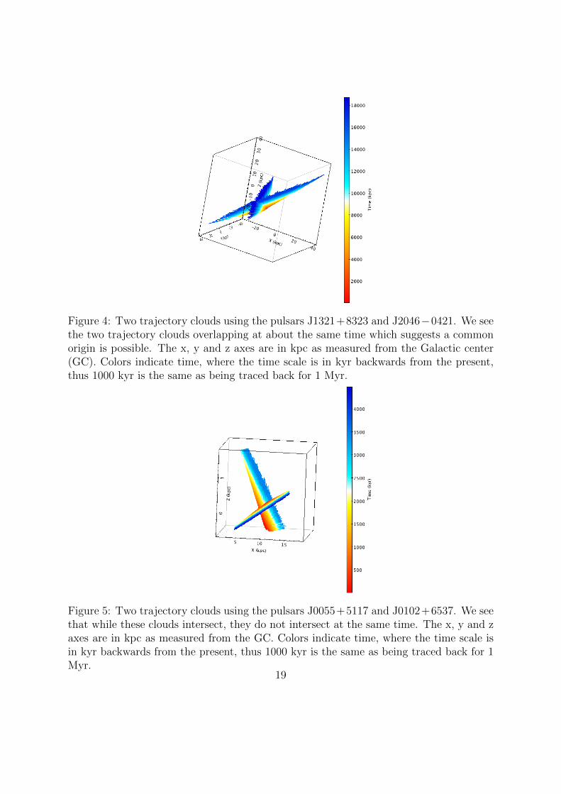
Figure 4: Two trajectory clouds using the pulsars J1321+8323 and J2046−0421. We seethe two trajectory clouds overlapping at about the same time which suggests a commonorigin is possible. The x, y and z axes are in kpc as measured from the Galactic center(GC). Colors indicate time, where the time scale is in kyr backwards from the present,thus 1000 kyr is the same as being traced back for 1 Myr.

Figure 5: Two trajectory clouds using the pulsars J0055+5117 and J0102+6537. We seethat while these clouds intersect, they do not intersect at the same time. The x, y and zaxes are in kpc as measured from the GC. Colors indicate time, where the time scale isin kyr backwards from the present, thus 1000 kyr is the same as being traced back for 1Myr.

19

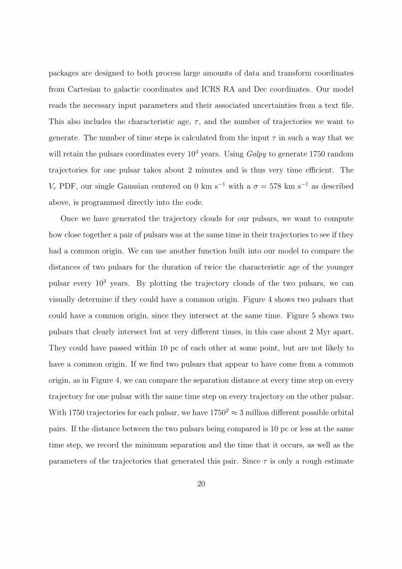
packages are designed to both process large amounts of data and transform coordinates

from Cartesian to galactic coordinates and ICRS RA and Dec coordinates. Our model

reads the necessary input parameters and their associated uncertainties from a text file.

This also includes the characteristic age, τ , and the number of trajectories we want to

generate. The number of time steps is calculated from the input τ in such a way that we

will retain the pulsars coordinates every 103 years. Using Galpy to generate 1750 random

trajectories for one pulsar takes about 2 minutes and is thus very time efficient. The

Vr PDF, our single Gaussian centered on 0 km s−1 with a σ = 578 km s−1 as described

above, is programmed directly into the code.

Once we have generated the trajectory clouds for our pulsars, we want to compute

how close together a pair of pulsars was at the same time in their trajectories to see if they

had a common origin. We can use another function built into our model to compare the

distances of two pulsars for the duration of twice the characteristic age of the younger

pulsar every 103 years. By plotting the trajectory clouds of the two pulsars, we can

visually determine if they could have a common origin. Figure 4 shows two pulsars that

could have a common origin, since they intersect at the same time. Figure 5 shows two

pulsars that clearly intersect but at very different times, in this case about 2 Myr apart.

They could have passed within 10 pc of each other at some point, but are not likely to

have a common origin. If we find two pulsars that appear to have come from a common

origin, as in Figure 4, we can compare the separation distance at every time step on every

trajectory for one pulsar with the same time step on every trajectory on the other pulsar.

With 1750 trajectories for each pulsar, we have 17502 ≈ 3 million different possible orbital

pairs. If the distance between the two pulsars being compared is 10 pc or less at the same

time step, we record the minimum separation and the time that it occurs, as well as the

parameters of the trajectories that generated this pair. Since τ is only a rough estimate

20

of age, it is of interest to note all times where the separation is ≤ 10 pc. We use 10 pc

as our maximum separation for a pair of successful trajectories consistent with previous

studies (Hoogerwerf et al., 2001, Vlemmings et al., 2004, Kirsten et al., 2015).

To trace back the trajectories of the OB Star Clusters, we use the same method for

the pulsars, utilizing Galpy and a Monte Carlo Method to generate 1750 trajectories.

An example trajectory cloud for one of of these OB associations is shown in Figure

6. When determining whether or not a pulsar could have come from a particular OB

Cluster, we use the same distance comparison method, counting only those trajectories

with separation of ≤ 10 pc between the pulsar and the center of these associations,

consistent with Hoogerwerf et al. (2001).

Figure 6: The trajectory cloud for the Upper Scorpius OB association. These OB associ-ation clouds are compared with pulsar trajectory clouds to determine if the pulsar couldhave been born there. The x, y and z axes are in kpc as measured from the GC. Colorsindicate time, where the time scale is in kyr backwards from the present, so 1000 kyr isthe same as being traced back for 1 Myr.

21

2.2.2 Using Galpy to Simulate Trajectories

The Galpy package (Bovy, 2015) integrates positions backwards based on present day

parameters RA, Dec, µ in RA (µα) and Dec (µδ), distance (d) from the Earth, and Vr. We

also specify the distance Earth is from the Galactic center (GC), (Ro). We use Ro = 8.27

kpc from Schonrich (2012) and the rotation velocity of the galaxy at Ro, which we have

specified as vo = 219.7 km s−1 from Vlemmings et al. (2004). We then can specify the

correction for the 3D solar motion relative to the local standard of rest. We do this

by specifying the 3D space velocity vectors according to the galactic coordinate system.

These 3D vectors as labeled U , V , and W respectively. We set U = 13.84, V = 12.24,

and W = 6.1 km s−1 also from Schonrich (2012).

Galpy can also account for the Milky Way’s gravitational potential. In particular

we use MWPotential2014, a composite potential with four different parts which is pre-

compiled in Galpy (Bovy, 2015). The first part of this potential is a Miyamoto-Nagai

Potential which accounts for the gravitational potential of the disk in the Milky Way

(Miyamoto & Nagai, 1975). The second part is a Navarro-Frenk-White (NFW) Poten-

tial which is the gravitational potential due to the dark matter halo in the Milky Way

(Navarro et al., 1996). The third component of MWPotential2014 is a a power-law density

spherical potential with an exponential cutoff (Bovy & Rix, 2013) which is the gravita-

tional potential of the central bulge of the Milky Way. The fourth component is a Kepler

Potential to account for the gravitational potential of the super massive black hole at

the center of the Milky Way, Sgr A∗, which is modeled in the potential as a point source

(Gillessen et al., 2009).

In order to determine if two pulsars were within 10 pc of each other at the same time

in their trajectory, we want to make sure the pulsars do not move more than 10 pc at

22

every time step. For this reason we use time steps of 103 yrs from the present day position

back through the trajectory to 2τ for all pulsars.

We override the default integrator in Galpy (“Scipy odeint”) and instead we use a

Fourth Order Runga-Kutta integration method, consistent with Kirsten et al. (2015)

and Hoogerwerf et al. (2001). When we compare the results of changing the integration

method, we obtain a difference of ∼ 15 successful orbits. This is a difference in our success

rate of only 0.0005%. We can therefore conclude that the method of integration does not

make a large difference in the overall method. Using Galpy to integrate the orbits and

then obtain the coordinates is not computationally expensive.

2.2.3 Initial Pair Tests

Since we are utilizing the new Python package Galpy, it is necessary to compare

our model with previously published results. We thus attempt to replicate the results

described in Hoogerwerf et al. (2001) of the runaway star ζ-Ophiuchi and the pulsar

B1929 + 10, as well as those described in Kirsten et al. (2015) for both the aforemen-

tioned pair and the pulsar pair B2020 + 28 and B2021 + 51. This pair of pulsars was

initially analyzed by Vlemmings et al. (2004), whose results we also compare our model

to.

ζ Ophiuchi and B1929+10

The pulsar and runaway star pair B1929 + 10 and ζ-Ophiuchi was first analyzed by

Hoogerwerf et al. (2001). These objects were originally traced back to a common origin in

the Upper Scorpius region approximately 1 Myr ago (Hoogerwerf et al., 2001). ζ-Ophiuchi

was previously found to have been a runaway star located in the Upper Scorpius Sco OB2

region about 1 Myr ago by de Zeeuw et al. (1999) who inferred that a supernova forced

23

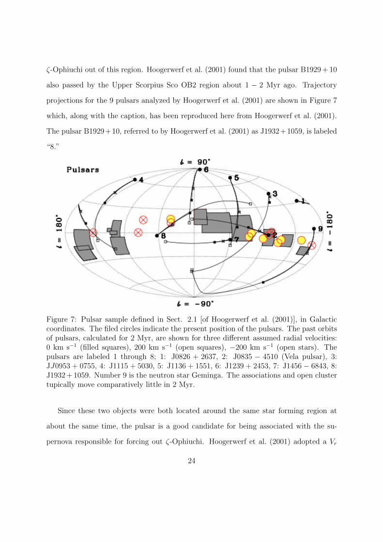
ζ-Ophiuchi out of this region. Hoogerwerf et al. (2001) found that the pulsar B1929 + 10

also passed by the Upper Scorpius Sco OB2 region about 1 − 2 Myr ago. Trajectory

projections for the 9 pulsars analyzed by Hoogerwerf et al. (2001) are shown in Figure 7

which, along with the caption, has been reproduced here from Hoogerwerf et al. (2001).

The pulsar B1929+10, referred to by Hoogerwerf et al. (2001) as J1932+1059, is labeled

“8.”

Figure 7: Pulsar sample defined in Sect. 2.1 [of Hoogerwerf et al. (2001)], in Galacticcoordinates. The filed circles indicate the present position of the pulsars. The past orbitsof pulsars, calculated for 2 Myr, are shown for three different assumed radial velocities:0 km s−1 (filled squares), 200 km s−1 (open squares), −200 km s−1 (open stars). Thepulsars are labeled 1 through 8; 1: J0826 + 2637, 2: J0835 − 4510 (Vela pulsar), 3:JJ0953 + 0755, 4: J1115 + 5030, 5: J1136 + 1551, 6: J1239 + 2453, 7: J1456 − 6843, 8:J1932 + 1059. Number 9 is the neutron star Geminga. The associations and open clustertupically move comparatively little in 2 Myr.

Since these two objects were both located around the same star forming region at

about the same time, the pulsar is a good candidate for being associated with the su-

pernova responsible for forcing out ζ-Ophiuchi. Hoogerwerf et al. (2001) adopted a Vr

24

distribution of 200 ± 50 km s−1 for the pulsar. They also doubled the uncertainties as-

sociated with the proper motions (Taylor et al., 1993) due to a possibility that they had

been underestimated (Campbell et al., 1996). Using the same Monte Carlo method we

have described, they simulated 3 million possible pairs of orbits for the two objects. In

addition to comparing the distance between the two objects, they also traced back the

trajectory of the Sco OB2 region and compared the distance of the two objects to the

center of this association.

In addition to Hoogerwerf et al. (2001), Kirsten et al. (2015) preformed the same

Monte Carlo simulation on B1929 + 10 and ζ-Ophiuchi using the same parameters. They

also adopted a galactic potential using the three part Staekel potential (Famaey & De-

jonghe, 2003) and solar motions from Schonrich (2012). Galpy does not have a Staekel

potential option, but it does have a Kuzmin-Kutuzov Staekel potential, which is a Galac-

tic potential which accounts for three integrals of motion (Dejonghe & de Zeeuw, 1988).

We initialize an approximate three part Staekel Potential in Galpy by setting three in-

dividual KuzminKutuzovStaekel potential objects and put them together in one list and

then use this list to make our galactic potential. This simulation by Kirsten et al. (2015)

was completed as part of a consistency check with Hoogerwerf et al. (2001) to attempt

to use the most recent, accurate measurements of the parameters of B1929 + 10 and

ζ-Ophiuchi to verify the initial results of Hoogerwerf et al. (2001).

Kirsten et al. (2015) also obtained new measurements for the parameters used to

trace ζ-Ophiuchi (van Leeuwen, 2007) and new astrometric parameters for B1929 + 10

(Kirsten et al., 2015) and compared the past results described above with those obtained

with the most recent astrometric values. Here, they use the same solar motions and

galactic potential as described above, but they adopt a bimodal Vr distribution for the

pulsar with peaks centered on ±400 km s−1 and standard deviations from these peaks

25

of 265 km s−1 shown in Figure 8. We adopt the same distribution picking the positive

and negative values by randomly picking values for Vr from a Gaussian centered on 400

km s−1 with σ = 265 km s−1 and then randomly assigning 50% of them a negative sign.

Kirsten et al. (2015) found that using the most recent astrometric measurements, it is

possible that their paths may have been close to each other about 0.5 Myr ago, but it

is unlikely that the two objects had either a common origin or originated in the Upper

Scorpius region.

1000 500 0 500 1000

Radial Velocity (km/s)

0.0

0.1

0.2

0.3

0.4

0.5

0.6

0.7

0.8

Pro

babili

ty D

ensi

ty (

10^

-3 p

er

km/s

)

Kirsten 2015 Radial Velocity PDF

Figure 8: A bimodal Vr PDF used by Kirsten et al. (2015) in their Monte Carlo pulsartrajectory simulations of the pulsars B1929 + 10, B2020 + 28, and B2021 + 51. They usea Gaussian PDF centered on 400 km s−1 with σ = 265 km s−1 and then randomly assigna positive or negative value to the chosen value. This is equivalent to selecting a Vr fromthe bimodal distribution shown here.

26

B2020+28 and B2021+51

We now consider the pair of pulsars, B2020 + 28 and B2021 + 51. These pulsars were

first traced back to a common origin within the Cygnus superbubble, near the Cyg OB2

region, approximately 2 Myr ago (Vlemmings et al., 2004). The characteristic ages of

B2020 + 28 and B2021 + 51 are 2.87 and 2.74 Myr respectively, which are both close

to 2 Myr. This pair is particularly interesting because the directions of the trajectories

of these two pulsars is directly opposite each other. This suggests that the progenitor

stars of these two pulsars were originally in a binary system with each other, which was

disrupted when the second star went supernova and the two resulting pulsars were sent

shooting away from each other (Vlemmings et al., 2004). We know that this cannot

have happened after the first supernova because the pulsars have a similar τ . This birth

scenario is shown in Figure 9 which has been reproduced, along with its caption, from

Vlemmings et al. (2004).

We attempted, but were unsuccessful, to replicate the radial velocity PDFs for the two

pulsars from the information given in Vlemmings et al. (2004) due to a lack of description

on the methods used to calculate the curves. However Vlemmings et al. (2004) reports

the peaks of the PDFs for B2020 + 28 and B2021 + 51 to be ±100 km s−1 and ±450 km

s−1 respectively. We thus estimate the Vr PDFs with a bimodal Gaussian with peaks at

±100 km s−1 for B2021 + 51 and a similar type of PDF for B2020 + 28 but with peaks

at ±450 km s−1. We then use our Monte Carlo Method to determine the number of

successful trajectories for B2020 + 28 and B2021 + 51.

In addition to analyzing the trajectories of B1929 + 10 and ζ-Ophiuchi, Kirsten et

al. (2015) also studied B2020 + 28 and B2021 + 51 since they had new astrometric mea-

surements for the pulsars. They again use the three-part Staekel Potential described

27

Figure 9: Three-dimensional pulsar motion through the Galactic potential for one ofthe pulsar orbit solutions that yields a minimum separation of less than 10 pc (theseparticular Galactic orbits cross within 4 pc). The dashed circle represents the CSB[Cygnus superbubble], while the labeled solid ellipses are the Cyg OB associations withpositions and extents as tabulated by Uyaniker et al. (2001). The extent of OB 2is unknown, and only the center of the association is indicated. The thick solid linesindicate the pulsar paths, with the origin denoted by the star and the arrows pointingin the direction of motion. The current positions are indicated by the filled circles. Theelliptical contours around the pulsars’ origin in these panels indicate the 1, 2, and 3 σlevels of the likelihood solution for the birth location for Galactic orbit solutions thatreach a minimum separation of less than 10 pc.

earlier. They use the same radial velocity distribution as in the previous simulation

with B1929 + 10 and ζ-Ophiuchi, shown in Figure 8. Their recent results suggest that

B2020+28 and B2021+51 were not born inside the Cygnus superbubble, but somewhere

outside of it, and gives the pulsars a much earlier time of closest approach, about 1.16+0.18−0.17

Myr ago. However they do not completely rule out a common origin for the two objects.

28

3 Initial Results

While we do not have new astrometric parameters for the pairs B1929 + 10 and ζ-

Ophiuchi and B2020 + 28 and B2021 + 51, we are interested in replicating the previous

results to verify our analysis method before using it to trace back the trajectories of the

44 PSRPI pulsars and determine their birth regions. In this section we present our results

in replicating the simulations done in Hoogerwerf et al. (2001), Vlemmings et al. (2004),

and Kirsten et al. (2015).

3.1 ζ Ophiuchi and B1929+10

We first present the results of our replication of the B1929 + 10 and ζ-Ophiuchi sim-

ulations. The π and µ values used to determine the trajectories for B1929 + 10 and

ζ-Ophiuchi are shown in Table 3. The parameters used for determining the trajectories

of this OB region, the Upper Scorpius region, (de Zeeuw et al., 1999) are shown in Table

2 denoted with the name “US”. We present a comparison of all of the simulations com-

pleted with all three sets of parameters in Table 4. These three set of parameters are those

from Hoogerwerf et al. (2001), van Leeuwen (2007), and Kirsten et al. (2015). The table

presents the number of separations of ≤ 10 pc between B1929 + 10 and ζ-Ophiuchi as

well as the number and percentage of successful trajectories to total trajectories between

B1929 + 10 and ζ-Ophiuchi and the Upper Scorpius (US) region.

29

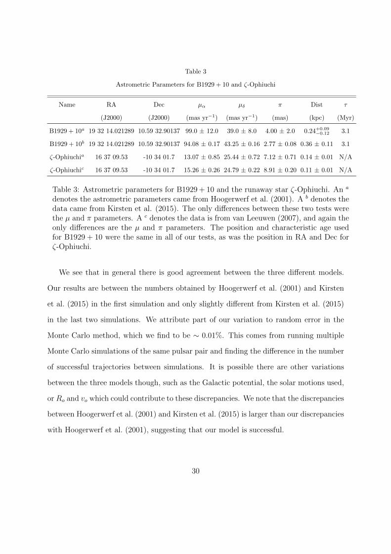
Table 3

Astrometric Parameters for B1929 + 10 and ζ-Ophiuchi

Name RA Dec µα µδ π Dist τ

(J2000) (J2000) (mas yr−1) (mas yr−1) (mas) (kpc) (Myr)

B1929 + 10a 19 32 14.021289 10.59 32.90137 99.0 ± 12.0 39.0 ± 8.0 4.00 ± 2.0 0.24+0.09−0.12 3.1

B1929 + 10b 19 32 14.021289 10.59 32.90137 94.08 ± 0.17 43.25 ± 0.16 2.77 ± 0.08 0.36 ± 0.11 3.1

ζ-Ophiuchia 16 37 09.53 -10 34 01.7 13.07 ± 0.85 25.44 ± 0.72 7.12 ± 0.71 0.14 ± 0.01 N/A

ζ-Ophiuchic 16 37 09.53 -10 34 01.7 15.26 ± 0.26 24.79 ± 0.22 8.91 ± 0.20 0.11 ± 0.01 N/A

Table 3: Astrometric parameters for B1929 + 10 and the runaway star ζ-Ophiuchi. An a

denotes the astrometric parameters came from Hoogerwerf et al. (2001). A b denotes thedata came from Kirsten et al. (2015). The only differences between these two tests werethe µ and π parameters. A c denotes the data is from van Leeuwen (2007), and again theonly differences are the µ and π parameters. The position and characteristic age usedfor B1929 + 10 were the same in all of our tests, as was the position in RA and Dec forζ-Ophiuchi.

We see that in general there is good agreement between the three different models.

Our results are between the numbers obtained by Hoogerwerf et al. (2001) and Kirsten

et al. (2015) in the first simulation and only slightly different from Kirsten et al. (2015)

in the last two simulations. We attribute part of our variation to random error in the

Monte Carlo method, which we find to be ∼ 0.01%. This comes from running multiple

Monte Carlo simulations of the same pulsar pair and finding the difference in the number

of successful trajectories between simulations. It is possible there are other variations

between the three models though, such as the Galactic potential, the solar motions used,

or Ro and vo which could contribute to these discrepancies. We note that the discrepancies

between Hoogerwerf et al. (2001) and Kirsten et al. (2015) is larger than our discrepancies

with Hoogerwerf et al. (2001), suggesting that our model is successful.

30

Table 4

Number of Successes for B1929 + 10 and ζ-Ophiuchi

Year of Parameters Hoogerwerf Hoogerwerf Kirsten Kirsten Our Model Our Model

According to et al. (2001) et al. (2001) et al. (2015) et al. (2015)

Citation Total Within US Total Within US Total Within US

B1929+10 (2001) 30822 4214 (0.14%) 37521 6816 (0.23%) 33242 5529 (0.18%)

ζ-Ophiuchi (2001)

B1929+10 (2001) 82840 (2.7%) 8 100109 (3.3%) 0

ζ-Ophiuchi (2007)

B1929+10 (2015) 258272 (8.6%) 0 246270 (8.0%) 0

ζ-Ophiuchi (2007)

Table 4: The results of the three sets of trajectory trace backs for B1929 + 10 and ζ-Ophiuchi using different sets of astrometric parameters. We report the number of orbitsthat had minimum separations of ≤ 10, or “successes”, pc between just B1929 + 10 andζ-Ophiuchi in the “Total” columns. In the columns labeled “Within US” we report thenumber of orbits that had minimum separations of ≤ 10 pc between B1929 + 10 andζ-Ophiuchi and the Upper Scorpius (US) region.

When we look at the simulations using the most recent astrometric parameters for

B1929+10, Kirsten et al. (2015) notes that most of the minimum separations were about

0.5 Myr ago and the smallest separation was 2.4 pc. The closest either B1929 + 10 or

ζ-Ophiuchi came to the center of the Upper Scorpius Region, Sco OB2, was 17 pc. Our

model resulted in all of our successful trajectories occurring between 0.25 and 1 Myr,

with neither the pulsar nor the star getting closer than 16 pc to Sco OB2. Similarly, we

find that our minimum separation between B1929 + 10 and ζ-Ophiuchi is 3.5 pc. These

specific results agree very well so can conclude that for this particular well-studied pair of

objects our model holds. However since the goals of this work are to look at pulsars with

a common origin, we now analyze a pulsar pair that has been traced back to a common

31

origin, B2020 + 28 and B2021 + 51.

3.2 B2020+28 and B2021+51

Similar to our comparison of B1929 + 10 and ζ-Ophiuchi, we will compare the Monte

Carlo trace back algorithm on the pulsars B2020 + 28 and B2021 + 51. We use the

parameters (Brisken et al., 2002, Kirsten et al., 2015) found in Table 5, and the same three-

part Staekel Potential and appropriate radial velocity PDFs described above. We present

our results along with those of the two different simulations, one using the parameters

from Vlemmings et al. (2004) and the other using parameters from Kirsten et al. (2015)

in Table 6. We do not compare the pulsar pair to a particular region. Thus we only look

at the number of separations of ≤ 10 pc between B2020 + 28 and B2021 + 51.

Table 5

B2020 + 28 and B2021 + 51 Astrometric Data

Name RA Dec µα µδ π Dist τ

(J2000) (J2000) (mas yr−1) (mas yr−1) (mas) (kpc) (Myr)

B2020 + 28a 20 22 37.0718 28 54 23.0300 -4.38 ± 0.53 -23.59 ± 0.26 0.37 ± 0.12 2.7+1.3−0.7 2.87

B2021 + 51a 20 22 49.8655 51 54 50.3881 -5.23 ± 0.17 11.54 ± 0.28 0.50 ± 0.07 2.0+0.3−0.2 2.74

B2020 + 28b 20 22 37.06758 28 54 22.7563 -3.34 ± 0.05 -23.65 ± 0.11 0.72 ± 0.03 1.63+0.50−0.23 2.87

B2021 + 51b 20 22 49.85890 51 54 50.5005 -5.08 ± 0.42 10.84 ± 0.25 0.80 ± 0.11 1.28+0.10−0.12 2.74

Table 5: Astrometric parameters for the two pulsars B2020 + 28 and B2021 + 51. An a

denotes the parameters came from Brisken et al. (2002). A b denotes the parameters camefrom Kirsten et al. (2015). The positions is in RA and Dec using the J2000 coordinatesystem. Our characteristic ages come from PSRCAT (Manchester et al., 2005).

32

Table 6

Number of Successes for B2020 + 28 and B2021 + 51

Parameters Vlemmings Kirsten Our Model

et al. (2004) et al. (2015)

(Year) (Total Successes) (Total Successes) (Total Successes)

2004 ≈ 0.15% 0.14% 2558 (0.08%)

2015 1866 (0.06%) 2201 (0.07%)

Table 6: The results of the two trace backs for B2020 + 28 and B2021 + 51. The numberof successful trajectories of all three models using parameters from Brisken et al. (2002)are shown in the first row. The number of successes using the parameters from Kirstenet al. (2015) are shown in the second row.

We can see in Table 6 that using the parameters from Brisken et al. (2002), Kirsten

et al. (2015) is able to obtain similar results as Vlemmings et al. (2004), but our results

are very different. While the random error in the Monte Carlo Method, as described in

section 3.1, along with possible differences in Galactic potential, solar motions, and other

implementation variables, could contribute to the apparent error, they cannot account for

a 0.07% difference. This simulation is the only one where we were unable to successfully

reconstruct the radial velocity PDF used. We believe that this significant difference is due

to mostly to our inability to reconstruct the radial velocity distributions of Vlemmings

et al. (2004). This suggests that the radial velocity distribution has a large effect on the

results of trajectory simulations for pulsars and thus that being able to more precisely

constrain the Vr for pulsars is very important if we want to find their birth sites.

We also attempted to replicate the Kirsten et al. (2015) trajectory trace back of

B2020 + 28 and B2021 + 51 using the new astrometric parameters and find our results to

be in reasonable agreement. Kirsten et al. (2015) found that their successful trajectories

33

crossed within 10 pc about 1.16+0.18−0.17 Myr ago with a minimum separation of 1.9 pc. We

obtain a similar number of trajectories crossing within 10 pc about 1.16+0.18−0.17 Myr ago with

a minimum separation of 0.4 pc. Our minimum separation is lower than that obtained by

Kirsten et al. (2015), however our results are generally in good agreement and the 0.01%

difference is easily explained by the systematic error in the Monte Carlo Method.

We were successfully able to replicated 4 of the 5 pulsar trace back simulations de-

scribed above. While we failed to replicate the results of Vlemmings et al. (2004) due to

our inability to replicate the Vr PDF, we can be confident that our model can accurately

trace back a pulsar through a galactic potential to locate a potential birth site.

34

4 Results of PSRPI Trajectories

We have simulated the trajectories of the 44 pulsars and 36 OB regions of interest.

We first looked at all 1128 possible pairs of pulsar trajectory clouds, as in Figure 4, to

determine the likelihood of common origins. We noted the pulsar trajectory clouds that

intersected, as in Figure 4, at approximately the same time, as shown by the color scale.

After looking at all possible pairs of pulsars, we looked at all 1584 of the combinations

of pulsars and regions and analyzed it similarly. An example of a pulsar trajectory cloud

with an OB region trajectory cloud is shown in Figure 10. We then analyzed these results

to see if any pulsars that likely came from the same region also had intersecting trajectory

clouds. Of the 1128 possible pulsar pairs, we found 16 that had the greatest likelihood

to have come from the same region at the same time. In each pair the pulsars had

similar characteristic ages and also similar ages to the OB region they were associated

with. Due to computational constraints we discuss only one such pair, J0102 + 6537 and

J0357 + 5236.

In addition to determining pulsars that may have a common origin, we look at likely

birth regions for all 44 pulsars individually as in Figure 10. We have identified likely OB

birth OB regions for 19 of the 44 pulsars within one of our 36 OB regions. We will discuss

only one of these associations, the pulsar J0055 + 5117 with the OB region Cas OB2.

4.1 Pulsar Pairs from the Same OB Region: J0102+6537 and

J0357+5236

We first discuss a pair of pulsars that we determined to have a likely common origin:

J0102 + 6537 and J0357 + 5236. We use the same criteria for identifying a successful

trajectory as in Vlemmings et al. (2004) and Kirsten et al. (2015), as described in Chapter

35

Figure 10: A close up of two example trajectory clouds using the pulsar J0102 + 6537and the OB region Cas OB2. The Cas OB2 trajectory cloud is the smaller cloud comingout of larger pulsar trajectory cloud. This shows the two trajectory clouds overlapping atabout the same time which suggests that the pulsar may have originated in this region.The x, y and z axes are in kpc as measured from the GC. The colors indicate time, wherethe scale is in kyr backwards from the present, so 1000 kyr is the same as being tracedback for 1 Myr.

2. We report the number of successful orbits along with the parameter distribution

and the Kolmogorov-Smirnov (KS) statistics comparing the distribution of successful

trajectory parameters to the overall distribution of Monte Carlo selected parameters for

the 1750 trajectories.

The trajectory clouds of these two pulsars are shown in Figure 11 and suggest a com-

mon origin since we have a clear intersection and the colors corresponding with time line

up. We find that 1092, or 0.035%, of our orbits result in separations of 10 pc or less.

This is a small number of successful trajectories when compared to the 30822 successful

trajectories obtained by Hoogerwerf et al. (2001) and ≈ 0.15% successful trajectories ob-

36

tained by Vlemmings et al. (2004). We also look at the successful parameter distributions

compared to the overall parameter distributions for J0102+6537 and J0357+5236 shown

in Figures 12 and 13, respectively. The KS statistic for each parameter of each pulsar is

shown in Table 7 along with the pulsar’s characteristic age.

Table 7

J0102 + 6537 and J0357 + 5236 KS Statistics and Age

Name π µα µδ τ (Myr)

J0102+6537 0.0605 0.0194 0.0407 4.42

J0357+5236 0.2152 0.0315 0.0370 6.55

Table 7: The KS statistics for the successful trajectory parameter distributions againstthe overall trajectory parameter distributions for J0102 + 6537 and J0357 + 5236. Welook at just the KS statistics for π and µ. Smaller KS values denote better correlationbetween the two distributions. We also list τ , in Myr, of each pulsar again for reference.

The KS statistic is the difference between the two distributions of parameters if they

had come from two separate PDFs. That is, a small KS value means there is a small

difference between the two PDFs and they are close to the same. In the context of this

work, this is the likelihood that our successful trajectories have the same parameter dis-

tributions as the overall parameter distributions. This allows us to statistically determine

if the successful trajectory parameters are skewed from the measured values of π and µ.

For most parameters we obtain a low KS statistic showing that our successful trajectory

results follow the measured parameters well, suggesting that the successful pairs show a

realistic birth scenario. The only large KS statistic is for the parallax of J0357 + 5236.

This tells us that for us to obtain a successful trajectory pair for J0102 + 6537 and

J0357 + 5236, the π value for J0357 + 5236 is more likely to be larger than the mean, or

37

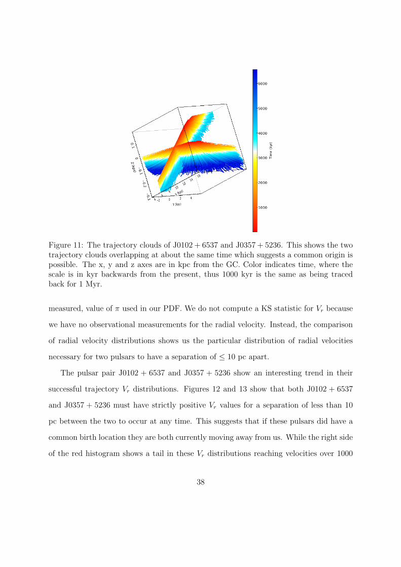
Figure 11: The trajectory clouds of J0102 + 6537 and J0357 + 5236. This shows the twotrajectory clouds overlapping at about the same time which suggests a common origin ispossible. The x, y and z axes are in kpc from the GC. Color indicates time, where thescale is in kyr backwards from the present, thus 1000 kyr is the same as being tracedback for 1 Myr.

measured, value of π used in our PDF. We do not compute a KS statistic for Vr because

we have no observational measurements for the radial velocity. Instead, the comparison

of radial velocity distributions shows us the particular distribution of radial velocities

necessary for two pulsars to have a separation of ≤ 10 pc apart.

The pulsar pair J0102 + 6537 and J0357 + 5236 show an interesting trend in their

successful trajectory Vr distributions. Figures 12 and 13 show that both J0102 + 6537

and J0357 + 5236 must have strictly positive Vr values for a separation of less than 10

pc between the two to occur at any time. This suggests that if these pulsars did have a

common birth location they are both currently moving away from us. While the right side

of the red histogram shows a tail in these Vr distributions reaching velocities over 1000

38

Figure 12: The Gaussian parameter distributions generated for J0102 + 6537 from ourMonte Carlo Method. The blue histograms are the overall parent distributions of theparameters for all 1750 trajectories. The red histograms are the distributions of theparameters for the successful trajectories. We see the Vr distribution in the upper left, πin the upper right, µα in the lower left, and µδ in the lower right.

39

Figure 13: The Gaussian parameter distributions generated for J0357 + 5236 from ourMonte Carlo Method. The blue histograms are the overall distributions of the parametersfor all 1750 trajectories. The red histograms are the distributions of the parameters forthe successful trajectories. The parameter distributions are the same as those in Figure12.

40

Figure 14: The left histogram shows the distribution of minimum trajectory separationsfor all 3 million possible orbits of J0102 + 6537 and J0357 + 5236. The blue shows everyminimum separation less than 1 kpc, and the red shows the separations ≤ 10 pc. Theright histogram shows the distribution of the time in the trajectory at which the minimumseparation between J0102+6537 and J0357+5236 occurred. τ for each pulsar is reportedin Table 7. The blue shows the time at which the minimum separation occurred for all3 million pairs, the red shows the time in the orbit at which the minimum separationoccured for pairs that had separations ≤ 10 pc.

km s−1 they peak at about 250 km s−1 and 300 km s−1 for J0102+6537 and J0357+5236

respectively. This shows us that if both of these pulsars did have a common birth OB

region, the most likely successful trajectories have radial velocities within a reasonable

range (∼ 100’s km s−1). If we infer that these pulsars are from the same origin, we can

then constrain Vr in future trajectory projections and simulations.

We also look at the distribution of the times at which the closest approaches of

J0102 + 6537 and J0357 + 5236 occur. The right side of Figure 14 shows the distribution

of the ages of the pulsars at every closest approach compared to the distribution of the

41

age of the pulsars when the closest approach was ≤ 10 pc. Here we note that most of the

closest approaches occurred between 1− 4 Myr, with more than half between 1− 3 Myr.

When we compare this time range with the characteristic ages of the pulsars, we see that

3 Myr is less than τ for J0102 + 6537 (4.47 Myr) and about half of τ for J0357 + 5236

(6.55 Myr). Since we know that τ is an imprecise way to measure the age of pulsar,

this does not immediately rule out a common origin for J0102 + 6537 and J0357 + 5236.

However, we would expect to find the time of closest approach to be closer to τ for both

pulsars for a true common origin (Vlemmings et al., 2004).

Finally, we compare J0102 + 6537 and J0357 + 5236 to the Cas OB2 region. We

find that 5710 of J0102 + 6537’s trajectories were within 10 of Cas OB2 at some point

in time, with the smallest separation being 0.04 pc. However, we find that only 21 of

J0357 + 5236’s trajectories are within 10 pc of Cas OB2 at some point in time, with the

smallest separation being 1.5 pc. These separation distributions are shown in Figure 15.

We also find that neither J0102 + 6537 nor J0357 + 5236 were both within 10 pc of Cas

OB2 at the same time. The low number of successful J0357 + 5236 trajectories, along

with the fact that we obtained no successful pairs of trajectories, show that it is highly

unlikely that J0102 + 6537 and J0357 + 5236 share a common origin in the Cas OB2

region.

The fact that J0102+6537 had 5710, ≈ 0.19%, successful trajectories and a minimum

separation of 0.04 from the center of Cas OB2 suggests that J0102 + 6537 may have been

born in Cas OB2. This number is similar to the number of successful trajectories in both

Vlemmings et al. (2004) and Hoogerwerf et al. (2001). However, if we look at Figure 16,

we see that all of the closest passes occurred between 1 and 2.5 Myr ago, which is less

than half of τ (4.47 Myr) for J0102 + 6537, and a quarter of the approximate age (10

Myr) of Cas OB2. This leads us to two possible scenarios.

42

10-4 10-3 10-2 10-1 100 101 102

Separation Distance (kpc)

0

100

101

102

103

104

105

106

Counts

J0102+6537 Separation Distribution to Cas_OB2

10-4 10-3 10-2 10-1 100 101 102

Separation Distance (kpc)

0

100

101

102

103

104

105

106

Counts

J0357+5236 Separation Distribution to Cas_OB2

Separation Distributions of J0102+6537 and J0357+5236 from Cas_OB2

Figure 15: The histrogram on the left shows the distribution of minimum separations lessthan 1 kpc between J0102 + 6537 and Cas OB2. The blue histogram shows the parentdistribution of all minimum separations for all trajectory pairs, while the red shows thedistribution for pairs with minimum separations ≤ 10 pc. The distributions on the rightshow the same results between J0357 + 5236 and Cas OB2.

0 2 4 6 8 10

Time of Min Separation (Myr)

0

100

101

102

103

104

105

106

107

Counts

J0102+6537 Time of Closest Seperation to Cas_OB2

0 2 4 6 8 10

Time of Min Separation (Myr)

0

100

101

102

103

104

105

106

107

Counts

J0357+5236 Time of Closest Seperation to Cas_OB2

Time of Minimum Separations of J0102+6537 and J0357+5236 from Cas_OB2

Figure 16: The histrogram on the left shows the distribuion of the time in the trajectoryat which the minimum separation occured between J0102+6537 and Cas OB2. The bluehistogram shows the time distribution of minimum separations for all trajectory pairs,while the red shows the time at which the a minimum separation of ≤ 10 pc occurredbetween J0102+6537 and Cas OB2. The distributions on the right show the same resultsfor J0357 + 5236 and Cas OB2. 43

The first scenario involves assuming that the characteristic age of J0102 + 6537 is

incorrect. If J0102 + 6537 is actually closer to 2 Myr old, then we can conclude that

Cas OB2 is the likely birth region of J0102 + 6537. The average lifetime of large O and

B stars is on the order of a few million years (Stothers, 1966). The ages of Cas OB2

and J0102 + 6537 suggest that it is likely that a large O or B star formed in Cas OB2

about 10 Myr ago, and could easily have exploded in a supernova a few million years ago

(Maeder & Meynet, 2000) producing a pulsar which is given a kick about 2.5 Myr ago. If

the progenitor star has a lifetime of only about 2 Myr (Savedoff, 1956) we could consider

8 Myr as an upper limit on the age of J0102 + 6537. The most likely birth scenario for

J0102+6537, therefore, is that a large O-type star in Cas OB2 exploded in an asymmetric

supernova about 5 − 8 Myr ago, and the core collapsed into a pulsar, J0102 + 6537, that

was then kicked out of the region (Dewey & Cordes, 1987) only 2.5 Myr ago.

The second scenario is that τ for J0102 + 6537 is correct and the pulsar was not born

in Cas OB2. This also has interesting implications, since it is still likely that J0102+6537

came near Cas OB2 ∼ 2 Myr ago. This would mean that J0102 + 6537 passed through

the Cas OB2 region. It is then possible that J0102 + 6537 may have had some kind of

interaction with another star in Cas OB2. Depending on the strength of this interaction,

the initial trajectory of J0102 + 6537 could have been altered. If there were a supernova

in the time that J0102 + 6537 passed through Cas OB2, J0102 + 6537 could have been

shot out of Cas OB2 imparting a large velocity to the pulsar (Iben & Tutukov, 1996).

There is no strong evidence to support either scenario to account for the past history

of J0102+6537 in our simulation, but it still presents interesting astrophysical possibilities

for stellar evolution. The likelihood of either of these scenarios is not well studied for

pulsars, and further studies of J0102 + 6537 and Cas OB2 as well as other similar pulsars

will allow us to learn more about the general population of neutron stars as well as

44

supernova dynamics.

Since it is unlikely that J0102 + 6537 and J0357 + 5236 had a common origin in Cas

OB2, we cannot use the successful trajectories shown in Figure 12 to limit J0102 + 6537

to just positive radial velocities. We were also unsuccessful in determining a birth region

for J0357 + 5236 in our model. We were, however, able to determine a possible birth

location for J0102 + 6537 and explore possible birth scenarios, although we are unable to

constrain the radial velocity parameter for J0102 + 6537. Through our analysis of this

pair we have shown that our method works well for determining which pairs of pulsars

and regions to analyze computationally.

4.2 Pulsar Pairs with No OB Region Matches

In our preliminary visual analysis of our pulsar trajectory clouds we also find 4 other

pulsars had possible common origins with other pulsars but did not have likely births

within our sample of OB regions. Table 8 lists these pulsars and their potential matching

pulsars. While we were not able to analyze these pulsars for likelihood of a common

origin, there are a few conclusions we can draw from this.

One possible reason for these apparent matches is that our first visual analysis was a

statistical coincidence due to the number of trajectories generated and uncertainties in the

initial parameters. If this is the case then these pulsars would not have any separations

less than 10 pc away from each other at the same time. Another consideration is that the

two pulsars do share a common origin, but that their progenitor stars were in an isolated

environment, possibly in a binary system with each other. However, while O stars can

be ejected from clusters, most are found within OB associations (Oh et al., 2015) so we

reject this scenario. The third possibility is that, even if the two pulsars do not share

45

a common origin, these pulsars originated in OB associations that are not within our

sample, which include only 36 of 140 different OB associations from Tetzlaff et al. (2010).

Table 8

Potential Pulsar Pairs without Associated Regions

Unassociated Pulsar Potential Pulsar Match

J0040+5716 J1257-1027

J1321+8323

J0826+2537 J1937+2544

J2113+2754

J2325+6316

J1257-1027 J1321+8323

J1607-0032

J2149+6329

J1919+0021 J0055+5117

Table 8: Pulsar pairs that were identified as possibly having a common origin but werenot found to have an association with any OB region from Table 2. Further analysis onthe other 104 OB associations (Tetzlaff et al., 2010) not analyzed in this work and these4 pulsars is required before any final conclusions about their origins can be made.

4.3 Pulsar Birth OB Regions: J0055+5117 and Cas OB2

We also use our method to determine if we can associate a pulsar with an OB association

as with J0102 + 6537 and Cas OB2. By looking at a pulsar trajectory cloud and a region

trajectory cloud, we can deduce if it is likely that the pulsar was born in that region, as

in Figure 10. Our analysis of pulsar birth OB regions is even more useful than looking

46

at the trajectory clouds of two pulsars together. If we are able to determine the birth

locations of many pulsars we can then see which pulsars were born in the same OB region

and use their characteristic ages together with the pulsar trajectory clouds, as in Figure

4, to determine the probability that the two pulsar could have related progenitor stars

(Vlemmings et al., 2004). This would reduce the number of pulsar pair trajectory clouds

that must be analyzed since we could determine that only certain pairs could have been

born within the same OB region. While we determined many likely pulsar birth regions,

due to computational restraints, we have only one relation to discuss at the time of this

writing.

One pulsar-OB region association suggested in our visual analysis was that of the

pulsar J0055 + 5117 and the OB region Cas OB2, whose trajectory clouds are both

shown in Figure 17. J0055 + 5117 has a τ = 3.51 Myr, well within the age (∼ 10 Myr) of

Cas OB2, further suggesting J0055 + 5117 could have been born in Cas OB2. When we

compute the actual separations between the trajectories of J0055 + 5117 and Cas OB2,

we find only 3 successful trajectories with separations less than 10 pc, and a minimum

separation of 5.2 pc. The distribution of separations between J0055 + 5117 and Cas OB2

less than 1 kpc are shown on the left side of Figure 18. We see from the right side of

Figure 18 that the time at which these 3 separations between J0055 + 5117 and Cas OB2

occurred was between 1−1.5 Myr ago. None of the minimum trajectory pair separations

occur later than 2 Myr ago, which is less than the characteristic ago of J0055 + 5117.

While we know that τ is imprecise, we expect many of the minimum separations between

two objects to occur nearer to the τ of the pulsar in question if it is likely to have been

born in that region. Additionally, just 3 successful trajectories is a value smaller than

the systematic differences in the Monte Carlo method itself. These results show that it

is extremely unlikely that J0055 + 5117 was born within the Cas OB2 association. We

47

did not find it likely that J0055 + 5117 was born within another cluster of OB stars in

our sample of 36 OB associations. However, we note that there are 104 OB regions in

the sample analyzed by Tetzlaff et al. (2010) we did not analyze.

Figure 17: The large, fan-shaped trajectory cloud for the pulsar J0055 + 5117 and thecone-shaped trajectory cloud of the Cas OB2 region. This shows the two trajectory cloudsoverlapping at about the same time which suggests that it is possible J0055 + 5117 couldhave been born in the Cas OB2 region. The x, y and z axes are in kpc as measured fromthe GC. Color indicates time, where the scale is in kyr backwards from the present, thus1000 kyr is the same as being traced back for 1 Myr.

48

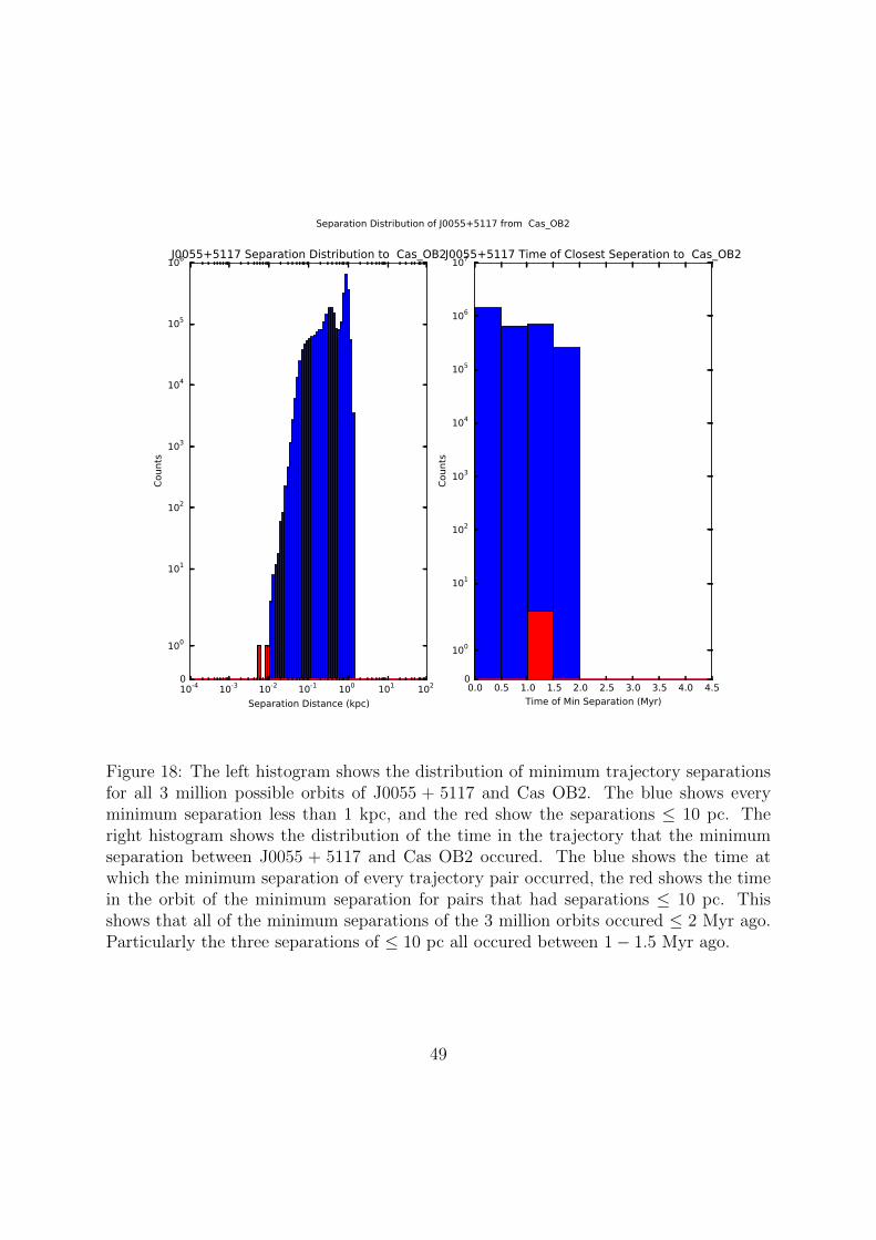
10-4 10-3 10-2 10-1 100 101 102

Separation Distance (kpc)

0

100

101

102

103

104

105

106

Counts

J0055+5117 Separation Distribution to Cas_OB2

0.0 0.5 1.0 1.5 2.0 2.5 3.0 3.5 4.0 4.5

Time of Min Separation (Myr)

0

100

101

102

103

104

105

106

107

Counts

J0055+5117 Time of Closest Seperation to Cas_OB2

Separation Distribution of J0055+5117 from Cas_OB2

Figure 18: The left histogram shows the distribution of minimum trajectory separationsfor all 3 million possible orbits of J0055 + 5117 and Cas OB2. The blue shows everyminimum separation less than 1 kpc, and the red show the separations ≤ 10 pc. Theright histogram shows the distribution of the time in the trajectory that the minimumseparation between J0055 + 5117 and Cas OB2 occured. The blue shows the time atwhich the minimum separation of every trajectory pair occurred, the red shows the timein the orbit of the minimum separation for pairs that had separations ≤ 10 pc. Thisshows that all of the minimum separations of the 3 million orbits occured ≤ 2 Myr ago.Particularly the three separations of ≤ 10 pc all occured between 1 − 1.5 Myr ago.

49

5 Conclusions

We have used our model to successfully trace back the trajectories of 44 pulsars in the

PSRPI survey and visually determine if they were likely to have a common origin. We

also traced back the trajectories of 36 OB regions and similarly visually determined the

likelihood that one of our pulsars had a likely origin in one of these OB regions. While

our model is only applicable for pulsars with τ . 30 Myr, this accounts for about 75%

of the PSRPI survey and a large number of pulsars that have already been discovered.

Our model is thus likely to be very useful for future studies looking into the determining

the birth regions of pulsars. As more astrometric measurements of young pulsars are

gathered we will be able to determine the likely birth regions of more pulsars. This in

turn can be cross correlated with previous pulsar-OB region associations. It will then be

possible, also using our model, to determine the likelihood that any pulsars coming from

the same OB region were associated with each other, or had progenitor stars associated

with each other, as in Vlemmings et al. (2004).

We were able to confirm the validity of our model, comparing it with previous results

from Hoogerwerf et al. (2001) and Kirsten et al. (2015) concerning B1929 + 10 and ζ-

Ophiuchi and from Vlemmings et al. (2004) and Kirsten et al. (2015) concerning B2020+

28 and B2021 + 51. Our comparisons returned similar numbers of successful trajectories

for both pairs of objects with the exception of Vlemmings et al. (2004). However, our

inability to replicate exactly the results of Vlemmings et al. (2004) shows the importance

of the Vr probability density function (PDF) used when tracing back pulsar trajectories,

since this was also the only simulation where we were not able to replicate the Vr PDF

exactly. Thus, being able to constrict the radial velocity of a pulsar is a critical part of

being able to determine an exact birth location of that pulsar. While the wide Gaussian

50

Vr PDF shown in Figure 3 allows us to account for the most reasonable values for a

pulsar’s radial velocity, it does not allow us to easily constrict the radial velocity of a

pulsar.

While we were not able to fully analyze every likely pulsar pair association or pulsar-

birth region association due to computational restraints, our analysis of the pulsars

J0102 + 6537 and J0357 + 5236 and the pulsar-OB region pair J0055 + 5117 and Cas

OB2 show promise for future studies. While J0102 + 6537 and J0357 + 5236 were not

found to have a common origin in Cas OB2, and that J0102+6537 was not likely born in

Cas OB2, we are able to propose two interesting possibilities for the history J0102+6537.

Similarly, in our analysis of J0055 + 5117 and Cas OB2, we found that it is extremely

unlikely that Cas OB2 is the birth region of J0055 + 5117. While we were unable to

determine a likely birth region for J0055 + 5117 from our sample of 36 OB associations,

we have narrowed down the possible birth regions for this pulsar. Through these two

possible pairs, this work has shown that our method is useful in determining likely birth

regions for pulsars.

The pulsars J0102+6537 and J0357+5236 and the pulsar-OB region pair J0055+5117

and Cas OB2 were just two comparisons that appeared to have promising results in our

preliminary visual analysis of the trajectory clouds. There are many more pairs of pulsars

and associated OB regions that suggested a common birth region for both pulsars that

we were not able to further analyze in this work. These other pulsar pairs and pulsar-OB

region associations can be found in Tables 9 and 10 respectively in Appendix A and will

be analyzed in future work.

In addition to future analysis of the pulsar-pulsar and pulsar-OB region associations

found in this initial study, there is much future work that can be done with the 44

PSRPI pulsars discussed in this work. Tetzlaff et al. (2010) looked at 140 different OB

51

associations as potential birth regions for just four young pulsars. Of these 140 different

OB associations, we analyzed only 36, just about 25% of the number of potential birth

OB regions we could have looked at. While this was due to computational constraints,

25 pulsars were found to have no likely birth OB regions within our sample of 36 OB

associations. In future work an analysis of the other 104 OB regions in Tetzlaff et al.

(2010) with the 44 pulsars of interest in this work could lead to determining the birth

regions for these pulsars as well.

Furthermore, this analysis method can be performed on pulsars yet to be discovered

and on pulsars with currently unknown astrometric parameters. We note as in Kirsten et

al. (2015) that the methods for measuring the astrometric parameters of pulsars, stars,

and even OB associations change and improve with the development of better techniques

and more sensitive instruments. Our model and the implementation of the Galpy package

allow us to easily recompute previously analyzed trajectories of astrophysical objects and

compare new results to previous results, as in Kirsten et al. (2015).

The implementation of the Galpy package and our Monte Carlo Method also allows

us to account for any future research in pulsar radial velocity PDFs, galactic potentials,

solar motions, and measurements of our own position in the Milky Way relative to the

Galactic Center. All of these measurements and models are utilized in our trace back

method and are easy to change within the model itself. This allows our model to produce

continually updated results while always using the most recent and accurate trajectory

parameters. The versatility of our model to include the most recent scientific discoveries

related to trajectory modeling allows it to be useful far into the future.

52

Acknowledgements

I would first like to thank my advisors at Cornell, Jim Cordes and Shami Chatterjee,

for helping me start this project and introducing me to world of pulsars. I would also like

to thank the NSF and the Cornell Astronomy REU program for giving me the wonderful

opportunity to work with Jim and Shami and the entire Astronomy Department. I would

like to thank my Union advisor Greg Hallenbeck, who made sure I actually turned my

thesis in. I would also like to thank Michael Warrener, who helped me with various sundry

computer and coding errors, and whose idea it was to use TOPCAT (Taylor, 2005) to

look at the pulsar trajectory clouds. My gratitude and thanks also goes to the entire

Union College Department of Physics and Astronomy for supporting me and helping me

find my passion for this field.

This material is based upon work supported by the National Science Foundation Re-

search Experience for Undergraduates program in Astronomy and Astrophysics at Cornell

University under Grant No. NSF/ AST-1156780. The National Radio Astronomy Obser-

vatory is a facility of the National Science Foundation operated under cooperative agree-

ment by Associated Universities, Inc. This work made use of the ATFN Pulsar Catalogue

(Manchester et al., 2005) found at http://www.atnf.csiro.au/people/pulsar/psrcat/.

53

6 Appendix A

In this appendix we present the pairs of pulsars from the PSRPI survey identified to

have a possible common origin that we were unable to analyze further than our prelimi-

nary visual trajectory cloud analysis in this work. The pulsar pairs along with the likely

OB regions are presented in Table 9.

We also present the pulsars that were connected to a possible birth OB region from

our sample of 36 OB associations that we were unable to further analyze. These pulsars

and any likely OB region associations are shown in Table 10. Both of these sets of results

show the success of our method in identifying possible pulsar pairs with a common origin

and also possible pulsar birth OB regions, thus significantly lowering the time necessary

for computations. We hope to analyze these results in the future.

54

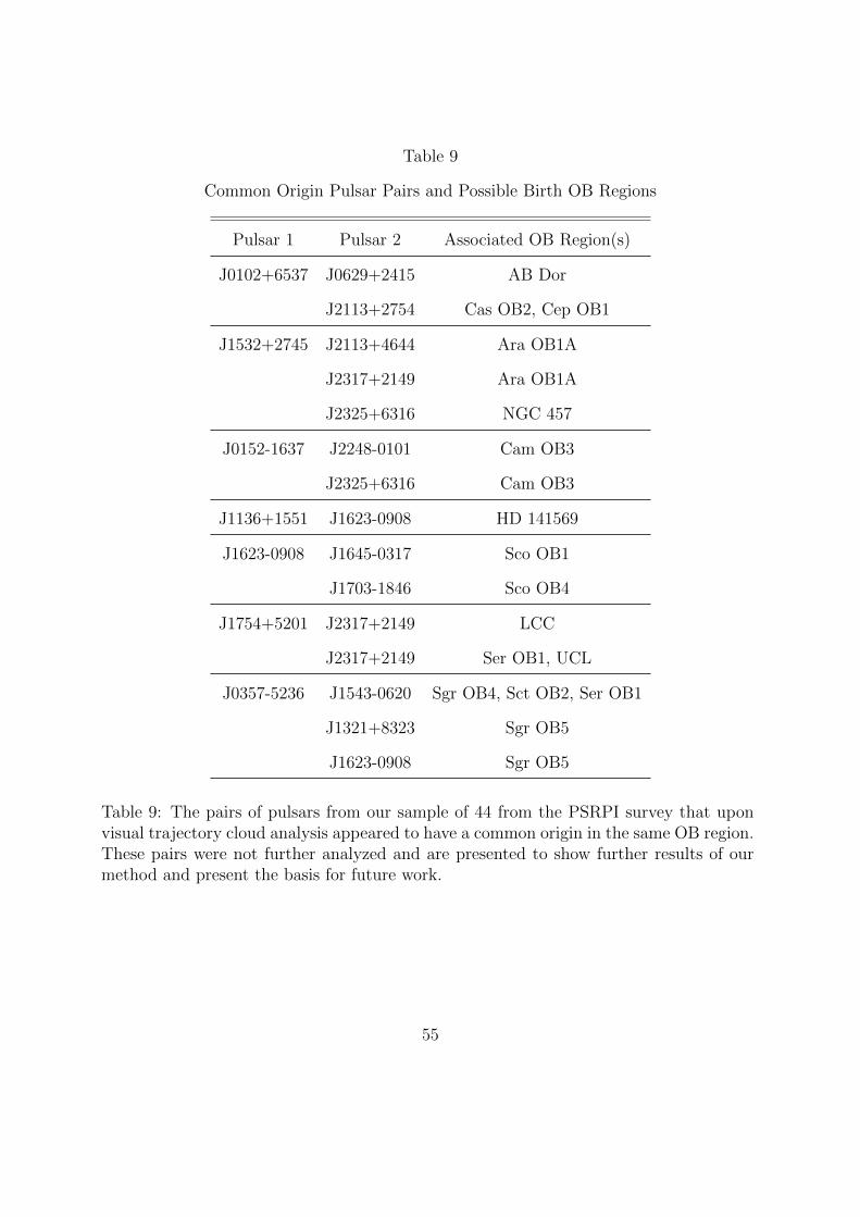
Table 9

Common Origin Pulsar Pairs and Possible Birth OB Regions

Pulsar 1 Pulsar 2 Associated OB Region(s)

J0102+6537 J0629+2415 AB Dor

J2113+2754 Cas OB2, Cep OB1

J1532+2745 J2113+4644 Ara OB1A

J2317+2149 Ara OB1A

J2325+6316 NGC 457

J0152-1637 J2248-0101 Cam OB3

J2325+6316 Cam OB3

J1136+1551 J1623-0908 HD 141569

J1623-0908 J1645-0317 Sco OB1

J1703-1846 Sco OB4

J1754+5201 J2317+2149 LCC

J2317+2149 Ser OB1, UCL

J0357-5236 J1543-0620 Sgr OB4, Sct OB2, Ser OB1

J1321+8323 Sgr OB5

J1623-0908 Sgr OB5

Table 9: The pairs of pulsars from our sample of 44 from the PSRPI survey that uponvisual trajectory cloud analysis appeared to have a common origin in the same OB region.These pairs were not further analyzed and are presented to show further results of ourmethod and present the basis for future work.

55

Table 10

Pulsar and Possible Birth OB Regions

Pulsar Associated OB Region(s)

J0102+6537 Cep OB1

J0152-1637 Cas OB2, NGC 457

J0357+5236 NGC 6530, Sgr OB4, Sgr OB5

J0629+2415 AB Dor, Ext R CrA, Gem OB1, Her-Lyr

J1136+1551 Cen OB1

J1321+8323 Sgr OB5

J1532+2745 Ara OB1A

J1543-0620 Sgr OB4

J1607-0032 ε Cha

J1623-0908 Sco OB1

J1645-0317 Sco OB1

J1754+5201 AB Dor, Her-Lyr, UCL

J2113+4644 AB Dor, Ara OB1A

J2248-0101 Cam OB1, NGC 457

J2305+3100 Cas OB2

J2317+2149 AB Dor, Ara OB1A

J2325+6316 Col 121, NGC 457

J2354+6155 Cas OB2

Table 10: The pulsars that showed possible birth OB regions within our sample of 36OB associations from Tetzlaff et al. (2010) that were not further analyzed in this work.These pairs represent a basis for future work.

56

References

Bisnovatyi-Kogan, G. S. 2006, Physics Uspekhi, 49, 53

Brisken, W. F., Benson, J. M., Goss, W. M., & Thorsett, S. E. 2002, ApJ, 571, 906

Bovy, J. 2015, ApJS, 216, 29

Bovy, J., & Rix, H.-W. 2013, ApJ, 779, 115

Campbell, R. M., Bartel, N., Shapiro, I. I., et al. 1996, ApJ, 461, L95

Chatterjee, S., Vlemmings, W. H. T., Brisken, W. F., et al. 2005, ApJ, 630, L61

Cordes, J. M. 1993, Planets Around Pulsars, 36, 43

Damour, T., & Taylor, J. H. 1992, Phys. Rev. D, 45, 1840

Davis, M. M., Taylor, J. H., Weisberg, J. M., & Backer, D. C. 1985, Nature, 315, 547

de Zeeuw, P. T., Hoogerwerf, R., de Bruijne, J. H. J., Brown, A. G. A., & Blaauw, A.

1999, AJ, 117, 354

Dejonghe, H., & de Zeeuw, T. 1988, ApJ, 333, 90

Deller, A. T., Brisken, W. F., Chatterjee, S., et al. 2011, 20th Meeting of the European

VLBI Group for Geodesy and Astronomy, held in Bonn, Germany, March 29-30, 2011,

Eds: W. Alef, S. Bernhart, and A. Nothnagel, Institut fur Geodasie und Geoinforma-

tion, Rheinischen Friedrich-Wilhelms-Universitat Bonn, p. 178-182, 178

Dewey, R. J., & Cordes, J. M. 1987, ApJ, 321, 780

Duncan, R. C., & Thompson, C. 1992, ApJ, 392, L9

57

Famaey, B., & Dejonghe, H. 2003, MNRAS, 340, 752

Ferrario, L., & Wickramasinghe, D. T. 2008, Astrophysics of Compact Objects, 968, 188

Gillessen, S., Eisenhauer, F., Fritz, T. K., et al. 2009, ApJ, 707, L114

Graham-Smith, F., & McLaughlin, M. A. 2005, Astronomy and Geophysics, 46, 1.23

Gott, J. R., III, Gunn, J. E., & Ostriker, J. P. 1970, ApJ, 160, L91

Hobbs, G., Lorimer, D. R., Lyne, A. G., & Kramer, M. 2005, MNRAS, 360, 974

Hoogerwerf, R., de Bruijne, J. H. J., & de Zeeuw, P. T. 2001, A&A, 365, 49

Hoyle, F., Fowler, W. A., Burbidge, G. R., & Burbidge, E. M. 1964, ApJ, 139, 909

Hulse, R. A., & Taylor, J. H. 1975, ApJ, 195, L51

Iben, I., Jr., & Tutukov, A. V. 1996, ApJ, 456, 738

Jacoby, B. A., Cameron, P. B., Jenet, F. A., et al. 2006, ApJ, 644, L113

Jenet, F., Finn, L. S., Lazio, J., et al. 2009, arXiv:0909.1058

Kirsten, F., Vlemmings, W., Campbell, R. M., Kramer, M., & Chatterjee, S. 2015, A&A,

577, A111

Kohler, S. 2015, AAS Nova Highlights, 248

Lai, D., Chernoff, D. F., & Cordes, J. M. 2001, ApJ, 549, 1111

Lam, M. T., Cordes, J. M., Chatterjee, S., et al. 2015, arXiv:1512.08326

Lorimer, D. R. 2008, Living Reviews in Relativity, 11,

58

Maeder, A., & Meynet, G. 2000, ARA&A, 38, 143

Manchester, R. N., Hobbs, G. B., Teoh, A., & Hobbs, M. 2005, VizieR Online Data

Catalog, 7245,

Miyamoto, M., & Nagai, R. 1975, ASJP, 27, 533

Navarro, J. F., Frenk, C. S., & White, S. D. M. 1996, ApJ, 462, 563

Oh, S., Kroupa, P., & Pflamm-Altenburg, J. 2015, ApJ, 805, 92

Richards, D. W., & Comella, J. M. 1969, Nature, 222, 551

Savedoff, M. P. 1956, ApJ, 124, 533

Schonrich, R. 2012, MNRAS, 427, 274

Stairs, I. H., Thorsett, S. E., Taylor, J. H., & Wolszczan, A. 2002, ApJ, 581, 501

Stothers, R. 1966, ApJ, 143, 91

Tauris, T. M. 1994, Proceedings of the Astronomical Society of Australia, 11, 82

Taylor, M. B. 2005, Astronomical Data Analysis Software and Systems XIV, 347, 29

Taylor, J. H., & Manchester, R. N. 1977, ARA&A, 15, 19

Taylor, J. H., Manchester, R. N., & Lyne, A. G. 1993, ApJS, 88, 529

Tetzlaff, N., Neuhauser, R., Hohle, M. M., & Maciejewski, G. 2010, MNRAS, 402, 2369

Turolla, R., Zane, S., & Watts, A. L. 2015, Reports on Progress in Physics, 78, 116901

van Leeuwen, F. 2007, Astrophysics and Space Science Library, 350,

59

Vlemmings, W. H. T., Cordes, J. M., & Chatterjee, S. 2004, ApJ, 610, 402

Weisberg, J. M., & Taylor, J. H. 2005, Binary Radio Pulsars, 328, 25

60