Modeling photosynthesis-irradiance curves: Effects of temperature, dissolved silica depletion, and changing community assemblage on community photosynthesis

424

Phytoplankton primary production plays a crucial role in arange of local and global phenomena. In the quest for under-standing the dynamics of algal growth and its associatedprocesses (nutrient uptake, temperature dependence, photo-acclimation, etc.), considerable effort is put into both datagathering and modeling. Two main approaches can be distin-guished: on the one hand, carefully designed laboratoryexperiments allow the growth of selected species to be studiedunder full control, and more or less complex dynamical mod-els are built and calibrated on the data set (e.g., Geider et al.1997; Davidson and Gurney 1999; Flynn and Martin-Jezequel2000). This approach increases our mechanistic understand-ing (Baklouti et al. 2006), although it is acknowledged thatexisting data sets are not adequate for the evaluation ofdetailed models (Flynn and Martin-Jezequel 2000). On theother hand, ecosystem scale studies of whole plankton com-munities are performed by incubating samples retrieved fromthe field at ambient conditions and varying light intensities E,

Modeling photosynthesis-irradiance curves: Effects oftemperature, dissolved silica depletion, and changingcommunity assemblage on community photosynthesisTom J. S. Cox1,2*, Karline Soetaert2, Jean-Pierre Vanderborght3, Jacco C. Kromkamp2, and Patrick Meire11University of Antwerp, Department of Biology, Ecosystem Management Research Group, Universiteitsplein 1, B-2610Antwerpen, Belgium2Netherlands Institute of Ecology (NIOO-KNAW), Centre for Estuarine and Marine Ecology, Korringaweg 7, P.O. Box 140, 4400AC Yerseke, The Netherlands3Université Libre de Bruxelles, Laboratory of Chemical Oceanography and Water Geochemistry, CP 208, Bd du Triomphe, B-1050, Bruxelles, Belgium

AbstractSets of photosynthesis-irradiance (P-I) curves yield more information about community photosynthesis

when analyzed with proper models in mind. Based on ecosystem-specific considerations regarding the factorsthat explain spatial and temporal patterns of photosynthesis, the Webb model of photosynthesis can be extend-ed and fitted to P-I data. We propose a method based on a series of nested models of increasing complexity totest whether supposed effects of environmental factors are reflected in the P-I data, whether more complexmodels fit the data significantly better than more simple models, and whether parameters describing the pre-sumed dependencies can be estimated from the data set. We compare a direct approach, fitting the extendedmodel to all P-I data at once, with a two-step approach in which photosynthetic efficiencies and maximum pho-tosynthetic rates of individual P-I curves are determined first, and then related to environmental variables. Anested model approach prevents overfitting of multiparameter models. Monte Carlo analysis sheds light on theerror structure of the model, by separating parameter and model uncertainty, and provides an assessment of theperformance of the formulations used in ecosystem models. We demonstrate that the two-step approach under-performs when used to compute photosynthetic rates. We apply the proposed method to an extensive P-I dataset from the Schelde estuary, where spatiotemporal patterns of photosynthesis arise from a combination of sea-sonality, silica depletion, phytoplankton community composition, and salinity effects.

*Corresponding author: E-mail: [email protected]

AcknowledgmentsMost of this work is financed by the Flemish Government,

Environment and Infrastructure department, AWZ, now NV WandZ (NVWaterwegen en Zeekanaal). The OMES monitoring and data manage-ment have been possible only by the continuous coordination effort ofStefan Van Damme and Tom Maris (University of Antwerp). We thankMarie Lionard (University of Ghent) for kindly providing the data oncommunity composition. We thank Didier Bajura (Université Libre deBruxelles [ULB]) for support in sampling. Dissolved silica concentrationswere determined by Lieve Clement and Eva De Bruyn in the Universityof Antwerp, Department of Biology, Testing Laboratory for ChemicalWater Quality. Michèle Loijens and Nathalie Roevros (ULB) are gratefullyacknowledged for performing 14C experiments and associated analyticaldeterminations. The data analysis and manuscript preparation was doneusing free software. We are grateful to the free software community forproviding such nice software as LaTeX, R, JabRef, and the Gimp. This ispublication 4835 of the NIOO-KNAW Netherlands Institute of Ecology.DOI 10.4319/lom.2010.8.424

Limnol. Oceanogr.: Methods 8, 2010, 424–440© 2010, by the American Society of Limnology and Oceanography, Inc.

LIMNOLOGYand

OCEANOGRAPHY: METHODS

Cox et al. Modeling photosynthesis-irradiance curves

425

and fitting a photosynthesis-irradiance (P-I) equation for everyindividual water sample. Next the spatiotemporal propertiesof the parameters of the P-I curve, of plankton production,and of the trophic status of the ecosystem are studied (e.g.Alpine and Cloern 1988; Keller 1988; Cole 1989; Kromkampand Peene 1995; MacIntyre and Cullen 1996; Goosen et al.1999; Gazeau et al. 2005; Goebel and Kremer 2007). Whereasthe former approach elucidates the mechanisms underlyingalgal growth, the performance of the models under (changing)ambient conditions is difficult to assess, since it is virtuallyimpossible to replicate all occurring natural situations in thelaboratory. Moreover, these single-species studies cannot sim-ply be translated to an ecosystem scale, where a succession ofseveral species is observed, each with different dynamics andsensitivities to environmental cues. In contrast, the latterapproach fully acknowledges the importance of natural vari-ability in algal community and environmental complexity,but fails in incorporating more detailed (mechanistic) knowl-edge in analyzing P-I data under varying temperature, nutri-ent availability, and community composition.

Usually, the relation of algal photosynthesis to environ-mental factors is studied in two steps. First, individual P-Icurves are fitted, which retrieves photosynthesis parameterssuch as photosynthetic efficiency and maximal photosynthe-sis rate. Second, these derived parameters are regressed againstenvironmental factors. In this article, we present two alterna-tive approaches for analyzing P-I measurements. In oneapproach, the direct procedure, parameters from an extendedWebb model (Webb et al. 1974) are estimated by fitting to allP-I and relevant environmental data at once. This extendedWebb model describes community photosynthesis as depend-ing on light and other environmental variables. In the secondapproach, the two-step procedure, the classic photosynthesisparameters α and Pm from each P-I curve are estimated first.Subsequently, these estimates are considered “observed data”and used to fit models that are derived from the models in thefirst approach. For both approaches, a series of nested modelsof increasing complexity is used to test whether the supposedeffects of environmental factors are reflected in the data,whether the more complex model fits the data significantlybetter, and whether the parameters describing the presumeddependencies can be estimated from the data set.

Such analyses would provide useful tools to study spa-tiotemporal patterns of community photosynthesis linked toenvironmental factors. In estuaries, for example, with a gradi-ent from saline to freshwater tidal reaches, such spatial vari-ability is pronounced. Concomitant with the abiotic gradient,the biological features such as algal community compositionand its properties change along the estuary (Kromkamp andPeene 1995; Muylaert et al. 2000; Goebel and Kremer 2007).Similarly, in both abiotic and biotic parameters, a strong sea-sonality is often observed, reflecting direct responses to ambi-ent temperatures but also resulting from seasonal successionof plankton species. Finally, periods of nutrient limitation

would influence community photosynthesis and potentiallybe reflected in observed P-I curves.

We apply the proposed methods to an extensive P-I data setfrom freshwater and brackish reaches of the Schelde estuary,gathered during 2003–2004. The monthly P-I determinationsalong the estuarine axis provide an elaborate data set of 151 P-I curve determinations totaling 1204 photosynthesis irradi-ance measurements. The system is known for its spatial gradi-ent, recurring silica depletion, and seasonal changes inphytoplankton community composition, and therefore thisdata set is ideally suited to assess and illustrate the subtletiesof the proposed methods. Accordingly, we demonstrate thateffects on community photosynthesis of seasonality, silicadepletion, and community composition lead to changes inthe P-I curve that are predictable to a certain extent. We com-pare the results of the direct and the two-step approaches,where we focus on their different performances for the calcu-lation of photosynthetic rates. The formulations we use arecommonly used in ecosystem model studies, although theyare mainly inspired by results of single-species experiments.Therefore we pay considerable attention to the interpretationof the results and their potential use. A Monte Carlo analysisof parameter and model uncertainty provides an assessment ofthe performance of the formulations used in model calcula-tions of ecosystem photosynthesis.

Materials and proceduresStudy area—The Schelde estuary is situated in Northern Bel-

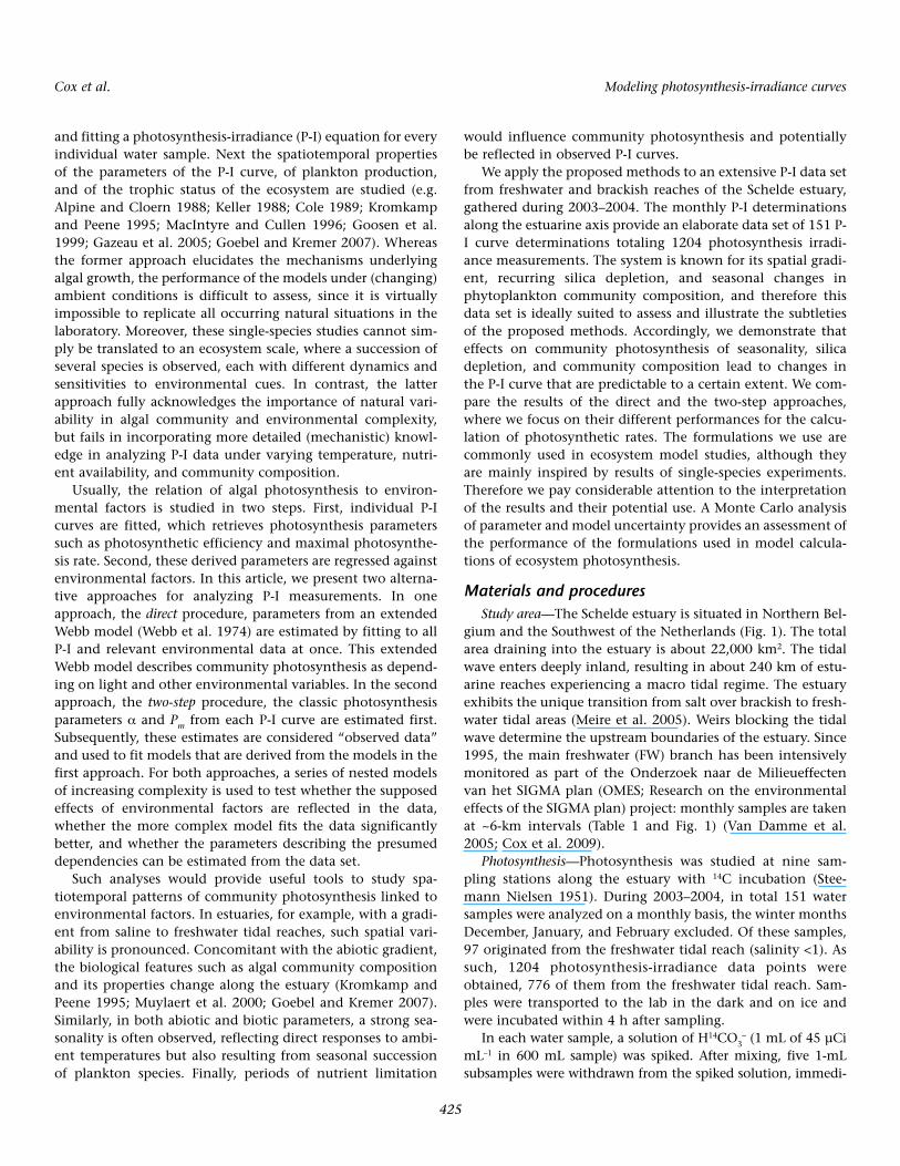
gium and the Southwest of the Netherlands (Fig. 1). The totalarea draining into the estuary is about 22,000 km2. The tidalwave enters deeply inland, resulting in about 240 km of estu-arine reaches experiencing a macro tidal regime. The estuaryexhibits the unique transition from salt over brackish to fresh-water tidal areas (Meire et al. 2005). Weirs blocking the tidalwave determine the upstream boundaries of the estuary. Since1995, the main freshwater (FW) branch has been intensivelymonitored as part of the Onderzoek naar de Milieueffectenvan het SIGMA plan (OMES; Research on the environmentaleffects of the SIGMA plan) project: monthly samples are takenat ~6-km intervals (Table 1 and Fig. 1) (Van Damme et al.2005; Cox et al. 2009).

Photosynthesis—Photosynthesis was studied at nine sam-pling stations along the estuary with 14C incubation (Stee-mann Nielsen 1951). During 2003–2004, in total 151 watersamples were analyzed on a monthly basis, the winter monthsDecember, January, and February excluded. Of these samples,97 originated from the freshwater tidal reach (salinity <1). Assuch, 1204 photosynthesis-irradiance data points wereobtained, 776 of them from the freshwater tidal reach. Sam-ples were transported to the lab in the dark and on ice andwere incubated within 4 h after sampling.

In each water sample, a solution of H14CO3– (1 mL of 45 µCi

mL–1 in 600 mL sample) was spiked. After mixing, five 1-mLsubsamples were withdrawn from the spiked solution, immedi-

Cox et al. Modeling photosynthesis-irradiance curves

426

ately treated with 500 µL NaOH 0.1 N, and analyzed for total14C activity (see below). The average from the five mea-surements was used as the initial 14C activity at the beginningof the incubation. At the same time, nine 50-mL subsampleswere taken and transferred into Corning incubation flasks forthe measurements of 14C uptake by phytoplankton. One of thesubsamples was used for the determination of dark 14C uptakeby autotrophs, and the other eight were placed in a four-rankincubator fixed on a shaking plate. Each rank held a series ofeight aligned flasks, the first being directly exposed to the lightsource (Sylvania Daylight F 8W/D); with this arrangement, thelight intensity decreased from the first to the eighth flask ineach rank. The irradiance was measured in the flasks using aquantum scalar irradiance meter (Biospherical Instruments QSL2100). Typical light profiles ranged from 400–500 to 20–50µmol photons m–2 s–1, depending on the water turbidity. Maxi-mal light intensity reflected the maximal in situ light availabil-ity. At the end of the incubation period (between 2 and 3 h), theflask contents were filtered on GF/F glass-fiber filters (pore size

0.7 µm). Filters were acidified with 100 µL HCl 0.1 N to elimi-nate the remaining bicarbonate before being dried and trans-ferred to scintillation vials. The 14C activity was determined in aliquid scintillation analyzer (Packard 1600 TR) after addition ofa scintillation cocktail (Ready Safe, Beckman Coulter).

Other laboratory methods—Chlorinity was determined col-orimetrically, from which salinity was calculated as S = 0.03 +1.805 * Cl [g L–1] (Unesco 1985). DSi samples were stored at4°C and analyzed by inductively coupled plasma optical emis-sion spectrometry (ICP-OES) within 24 h after sampling. Aver-age winter (Dec–Feb) DSi concentration in the FW tidalreaches amounted to 247 µM in 2003 and 253 µM in 2004,whereas the observed minima in summer were 1.3 and 0.8µM, respectively. DSi concentrations <10 µM, taken as a con-servative upper limit for possible silica limitation (Martin-Jeze-quel et al. 2000), were observed in both years in an extendedpart of the FW tidal reaches (Fig. 2A). In situ measured tem-perature displayed a clear seasonality (Fig. 2B): mean winter(summer) temperature in 2003 was 5.8°C (22.7°C) and 6.4°C

Fig. 1. The Belgian part of the Schelde estuary with its tributaries and major cities. Numbers indicate the sampling stations of the OMES monitoringcampaign. Encircled numbers indicate stations where photosynthetic rates were determined.

Cox et al. Modeling photosynthesis-irradiance curves

427

(20.9°C) in 2004.Except for June–October 2003, chlorophyll a (chl a) con-

centrations (Fig. 3C) were determined with HPLC analysis.Sampled water (250–500 mL) was filtered over a GF/F glass fiberfilter (Whatmann). Filters were wrapped in aluminum foil andstored on ice during transport and at –80°C in the lab. Pig-ments were extracted in 90% acetone by means of sonication(tip sonicator, 40 W for 30 s). Pigment extracts were filteredover a 0.2-µm nylon filter and injected into a Gilson HPLC sys-tem equipped with an Alltima reverse-phase C18 column (25cm × 4.6 mm, 5 µm particle sizes). Pigments were analyzedaccording to Wright and Jeffrey (1997). This method uses a gra-dient of three solvents: methanol 80%–ammonium acetate20%, acetonitrile 90%, and ethyl acetate. We used an AppliedBiosystems 785A detector to measure absorbance at 685 nm, aGilson model 121 fluorometer to measure fluorescence ofchlorophylls and their derivates, and a Gilson 170 diode arraydetector to measure absorbance spectra for individual pigmentpeaks. Pigments were identified by comparison of retentiontimes and absorption spectra with pure pigment standards.

June–October 2003 chl a concentrations were determinedfluorometrically. Phytoplankton cells were collected by filtra-tion on GF/F glass fiber filters (nominal pore size 0.7 µm) andwere then deep-frozen and kept in the dark at –15°C. Chloro-

Table 1. The OMES monitoring stations.

Name Number Distance, km Salinity

Boei 87a 1 58 9.5Boei 92 2 63.5 6.6Boei 105 3 71 4.1Antwerpen 4 78 2.0Kruibekea 5 85 0.80Bazel 6 89 0.53Steendorp 7 94 0.40Temsea 8 98.5 0.30Mariekerkea 9 107 0.20Vlassenbroek 10 118 0.18Dendermondea 11 121 0.17St-Onolfs 12 125 0.17Appelsa 13 128 0.17Uitbergena 14 138 0.17Wetteren 15 145 0.17Mellea 16 151 0.17

The distance is from the mouth of the estuary (Vlissingen, Netherlands).Salinity is the 2003–2004 average.aStations where photosynthesis parameters were determined.

Fig. 2. Kriging interpolation plot of dissolved silica concentration (A), fraction of diatoms in the algal population (B), and seasonal variation of watertemperature (C) as measured during the OMES measurement campaigns of 2003–2004. Individual samples are marked with gray +. Dissolved silica con-centrations <10 µM, which can possibly indicate silica limitation of diatom growth, are marked with a black dot. Distance refers to kilometers from themouth of the estuary.

Cox et al. Modeling photosynthesis-irradiance curves

428

phyll a determination was performed by fluorescence accord-ing to the procedure introduced by Yentsch and Menzel (1963),adapted by Strickland and Parsons (1972). Pigments wereextracted with 90% acetone. A Shimadzu RF-1501 fluorometerwas used for pigment analysis (excitation at 430 nm, emissionat 670 nm). Correction for (and calculation of) phaeopigmentswas achieved by successive measurements before and afteraddition of 100 µL HCl (0.1 M). The procedure was calibratedby means of pure chl a extract (Sigma-Aldrich).

The CHEMTAX algorithm (Mackey et al. 1996) was used todistinguish between diatom and other algal groups’ contribu-tion to total chl a, using concentrations of accessory pig-ments. The initial pigment ratio matrix was based on pub-lished accessory pigment to chl a ratios in estuaries (Lewitus etal. 2005; Schlüter et al. 2000), as well as measured from cul-tures of major diatoms (Cyclotella scaldensis and Stephanodiscushantzschii) isolated in the freshwater reaches of the Scheldeestuary (Lionard et al. 2008). The relative contribution ofdiatoms to chl a in the FW tidal reaches varied between 22%and 97% (Fig. 2). The fraction of diatoms was highest in sum-mer (on average 81% in 2003 and 73% in 2004) and lowest inwinter (on average 47% in 2003 and 57% in 2004).

Statistical methods—Direct and two-step approaches: Thestarting point of the analysis of the P-I data is the Webb model(Webb et al. 1974), relating (algal) photosynthesis (P) to inci-dent light intensity (E):

(1)

in which the independent variable vector x0 = [E] and theparameter vector θθ0 = [α, Pm]; Pm is the maximum photosyn-thetic rate [gC (gChl . h)–1], and α the photosynthetic effi-ciency [gC (gChl h)–1/µmol photons (m2 . s)–1].

Classically, this model is fitted on individual observed pho-tosynthesis-irradiance curves. When a collection of such datais available, the resulting set of parameters α and Pm can beused to study spatiotemporal variation of photosynthesis. Wewill call this the two-step approach. Usually, simple linear tech-niques (ANOVA, regression, principal components analysis[PCA]) are used to study the variation in the α and Pm esti-mates and their relation with abiotic factors (e.g., Kromkampand Peene 1995; MacIntyre and Cullen 1996; Goebel and Kre-mer 2007). In contrast, we propose to extend the Webb model(Eq. 1), based on ecosystem-specific considerations regardingthe factors that explain spatial and temporal patterns of pho-tosynthesis. Among others, such factors could include tem-perature, nutrient availability, photo-acclimation, and chang-ing phytoplankton species composition due to seasonalsuccession or selective grazing pressure. When we denote suchan extended Webb model by Pi(xi,θθi), with xi the vector ofexplanatory variables and θθi the parameter vector of thismodel, the corresponding models for α and Pm are given by

(2)

(3)

As such, the parameters of the extended Webb model can beestimated by fitting these models on the α and Pm determinedin the first step. Note that the α and Pm equations haveparameters in common. When fitted separately, the obtainedparameter estimates will be specific for either α or Pm. Alter-natively, a weighted least squares fit can be performed whereone set of parameters is estimated based on the combined setof α and Pm values, weighted by their standard deviations. Wewill denote the two alternatives by separate and joint two-stepfit, respectively.

The two-step approach above is close to the classicapproach of analyzing sets of P-I data, and can be seen as anextension from linear to (well-chosen) nonlinear models relat-ing photosynthesis to environmental factors. In addition weintroduce the direct approach, in which extended Webb mod-els Pi(xi,θθi) are fitted directly on the whole set of photosyn-thesis-irradiance points and environmental data, instead offirst determining α and Pm from each P-I curve and then fittingthe models 2 and 3.

Assessing model performance: Next we describe some sta-tistical tools to assess the performance of the models used andthe reliability of the parameter estimates obtained and theirstatistics, and to clarify the error structure of the models. Wewill particularly be dealing with sequences of nested models

P Pim i iE

i i( , ) lim ( , )x xθθ θθ=→∞

α( , )( , )

xx

i ii i

E

dPi

dEθθ

θθ=

=0

P PE

Pm

m

0 10 0( , ) exp.

x θθ = × −−

α

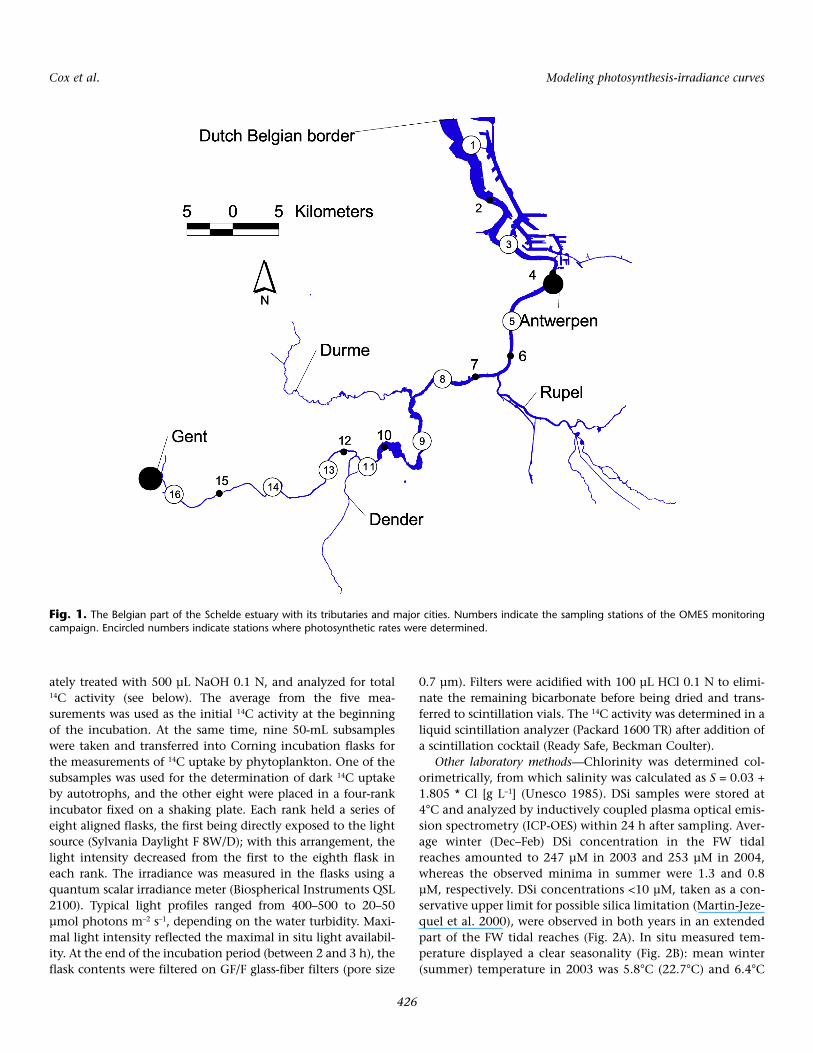
Fig. 3. Residuals versus the predicted values of the model P0. Untrans-formed (inset) and log-transformed (main figure).

Cox et al. Modeling photosynthesis-irradiance curves

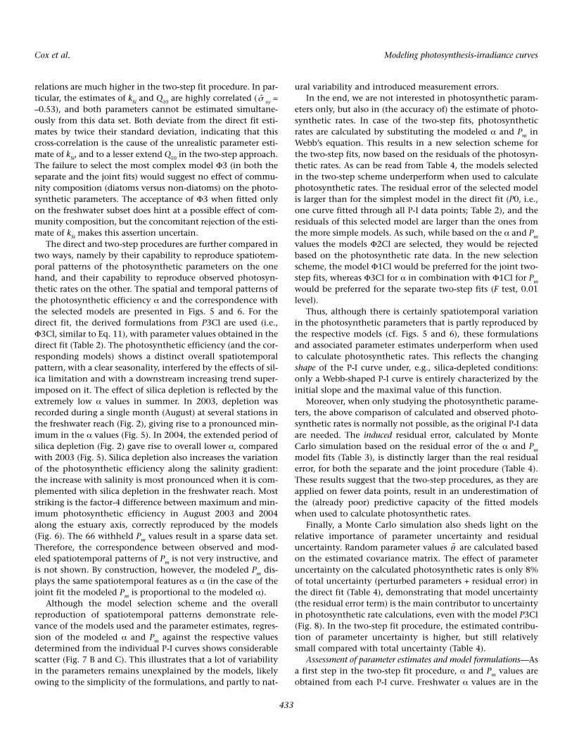
429

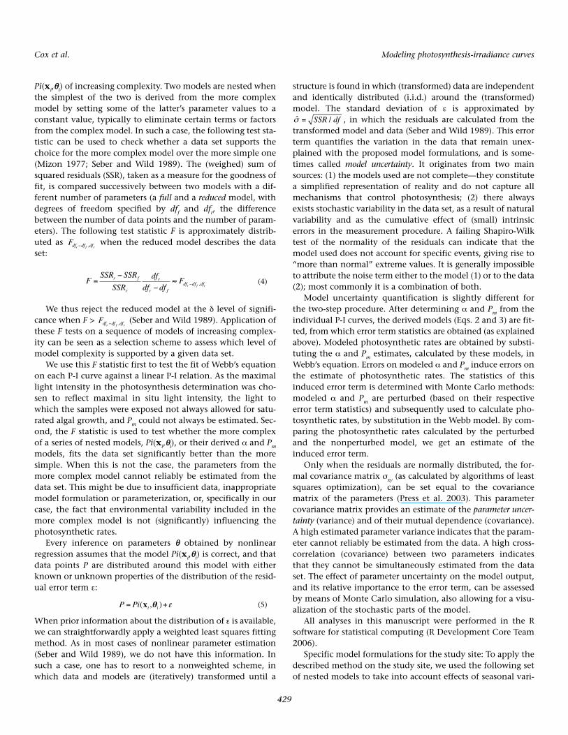
Pi(xi,θθi) of increasing complexity. Two models are nested whenthe simplest of the two is derived from the more complexmodel by setting some of the latter’s parameter values to aconstant value, typically to eliminate certain terms or factorsfrom the complex model. In such a case, the following test sta-tistic can be used to check whether a data set supports thechoice for the more complex model over the more simple one(Mizon 1977; Seber and Wild 1989). The (weighed) sum ofsquared residuals (SSR), taken as a measure for the goodness offit, is compared successively between two models with a dif-ferent number of parameters (a full and a reduced model, withdegrees of freedom specified by dff and dfr, the differencebetween the number of data points and the number of param-eters). The following test statistic F is approximately distrib-uted as when the reduced model describes the dataset:

(4)

We thus reject the reduced model at the δ level of signifi-cance when F > (Seber and Wild 1989). Application ofthese F tests on a sequence of models of increasing complex-ity can be seen as a selection scheme to assess which level ofmodel complexity is supported by a given data set.

We use this F statistic first to test the fit of Webb’s equationon each P-I curve against a linear P-I relation. As the maximallight intensity in the photosynthesis determination was cho-sen to reflect maximal in situ light intensity, the light towhich the samples were exposed not always allowed for satu-rated algal growth, and Pm could not always be estimated. Sec-ond, the F statistic is used to test whether the more complexof a series of nested models, Pi(xi,θθi), or their derived α and Pm

models, fits the data set significantly better than the moresimple. When this is not the case, the parameters from themore complex model cannot reliably be estimated from thedata set. This might be due to insufficient data, inappropriatemodel formulation or parameterization, or, specifically in ourcase, the fact that environmental variability included in themore complex model is not (significantly) influencing thephotosynthetic rates.

Every inference on parameters θθ obtained by nonlinearregression assumes that the model Pi(xi,θθi) is correct, and thatdata points P are distributed around this model with eitherknown or unknown properties of the distribution of the resid-ual error term ε:

(5)

When prior information about the distribution of ε is available,we can straightforwardly apply a weighted least squares fittingmethod. As in most cases of nonlinear parameter estimation(Seber and Wild 1989), we do not have this information. Insuch a case, one has to resort to a nonweighted scheme, inwhich data and models are (iteratively) transformed until a

structure is found in which (transformed) data are independentand identically distributed (i.i.d.) around the (transformed)model. The standard deviation of ε is approximated by

, in which the residuals are calculated from thetransformed model and data (Seber and Wild 1989). This errorterm quantifies the variation in the data that remain unex-plained with the proposed model formulations, and is some-times called model uncertainty. It originates from two mainsources: (1) the models used are not complete—they constitutea simplified representation of reality and do not capture allmechanisms that control photosynthesis; (2) there alwaysexists stochastic variability in the data set, as a result of naturalvariability and as the cumulative effect of (small) intrinsicerrors in the measurement procedure. A failing Shapiro-Wilktest of the normality of the residuals can indicate that themodel used does not account for specific events, giving rise to“more than normal” extreme values. It is generally impossibleto attribute the noise term either to the model (1) or to the data(2); most commonly it is a combination of both.

Model uncertainty quantification is slightly different forthe two-step procedure. After determining α and Pm from theindividual P-I curves, the derived models (Eqs. 2 and 3) are fit-ted, from which error term statistics are obtained (as explainedabove). Modeled photosynthetic rates are obtained by substi-tuting the α and Pm estimates, calculated by these models, inWebb’s equation. Errors on modeled α and Pm induce errors onthe estimate of photosynthetic rates. The statistics of thisinduced error term is determined with Monte Carlo methods:modeled α and Pm are perturbed (based on their respectiveerror term statistics) and subsequently used to calculate pho-tosynthetic rates, by substitution in the Webb model. By com-paring the photosynthetic rates calculated by the perturbedand the nonperturbed model, we get an estimate of theinduced error term.

Only when the residuals are normally distributed, the for-mal covariance matrix σxy (as calculated by algorithms of leastsquares optimization), can be set equal to the covariancematrix of the parameters (Press et al. 2003). This parametercovariance matrix provides an estimate of the parameter uncer-tainty (variance) and of their mutual dependence (covariance).A high estimated parameter variance indicates that the param-eter cannot reliably be estimated from the data. A high cross-correlation (covariance) between two parameters indicatesthat they cannot be simultaneously estimated from the dataset. The effect of parameter uncertainty on the model output,and its relative importance to the error term, can be assessedby means of Monte Carlo simulation, also allowing for a visu-alization of the stochastic parts of the model.

All analyses in this manuscript were performed in the Rsoftware for statistical computing (R Development Core Team2006).

Specific model formulations for the study site: To apply thedescribed method on the study site, we used the following setof nested models to take into account effects of seasonal vari-

Fdf df dfr f r− ,

FSSR SSR

SSR

df

df dfFr f

r

r

r f

df df dfr f r=

−

−≈ − ,

Fdf df dfr f r− ,

P Pi i i= +( , )x θθ ε

ˆ /σ = SSR df

Cox et al. Modeling photosynthesis-irradiance curves

430

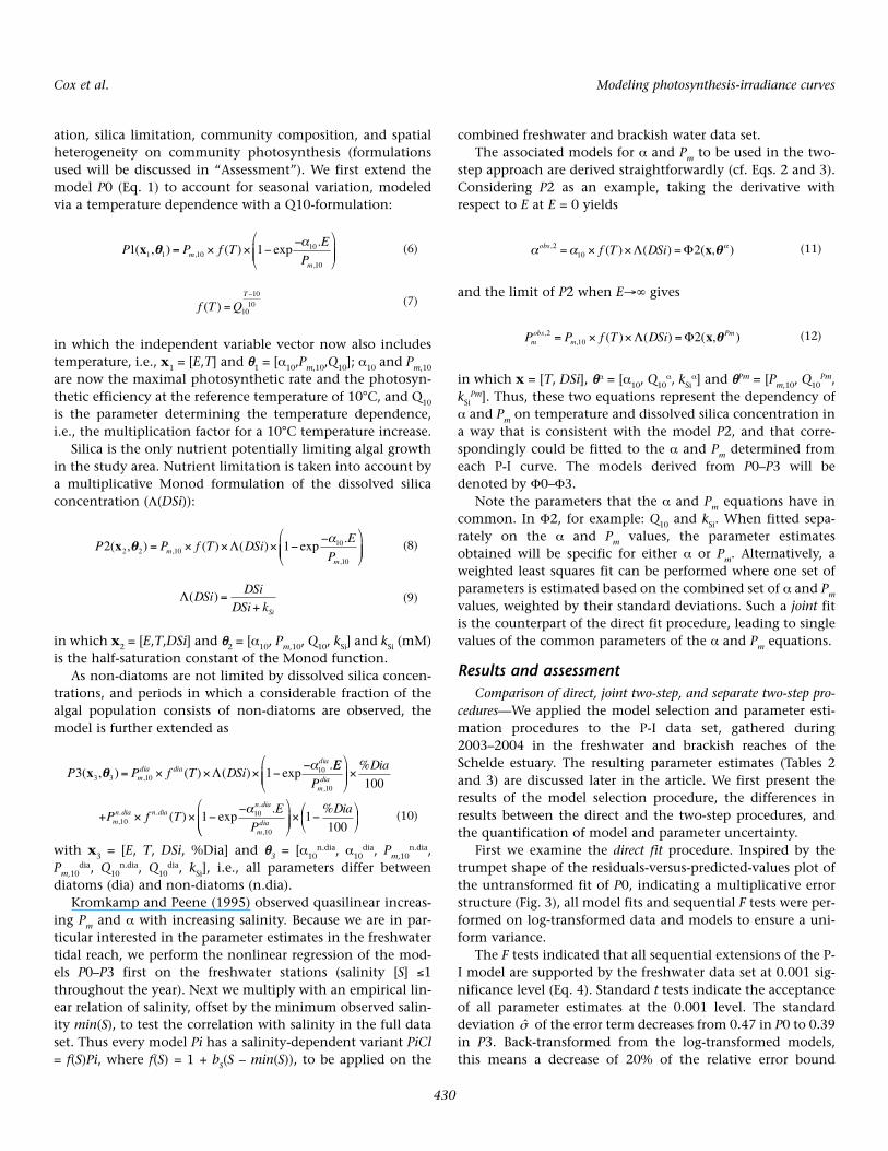
ation, silica limitation, community composition, and spatialheterogeneity on community photosynthesis (formulationsused will be discussed in “Assessment”). We first extend themodel P0 (Eq. 1) to account for seasonal variation, modeledvia a temperature dependence with a Q10-formulation:

(6)

(7)

in which the independent variable vector now also includestemperature, i.e., x1 = [E,T] and θθ1 = [α10,Pm,10,Q10]; α10 and Pm,10

are now the maximal photosynthetic rate and the photosyn-thetic efficiency at the reference temperature of 10°C, and Q10

is the parameter determining the temperature dependence,i.e., the multiplication factor for a 10°C temperature increase.

Silica is the only nutrient potentially limiting algal growthin the study area. Nutrient limitation is taken into account bya multiplicative Monod formulation of the dissolved silicaconcentration (Λ(DSi)):

(8)

(9)

in which x2 = [E,T,DSi] and θθ2 = [α10, Pm,10, Q10, kSi] and kSi (mM)is the half-saturation constant of the Monod function.

As non-diatoms are not limited by dissolved silica concen-trations, and periods in which a considerable fraction of thealgal population consists of non-diatoms are observed, themodel is further extended as

(10)

with x3 = [E, T, DSi, %Dia] and θθ3 = [α10n.dia, α10

dia, Pm,10n.dia,

Pm,10dia, Q10

n.dia, Q10dia, kSi], i.e., all parameters differ between

diatoms (dia) and non-diatoms (n.dia).Kromkamp and Peene (1995) observed quasilinear increas-

ing Pm and α with increasing salinity. Because we are in par-ticular interested in the parameter estimates in the freshwatertidal reach, we perform the nonlinear regression of the mod-els P0–P3 first on the freshwater stations (salinity [S] ≤1throughout the year). Next we multiply with an empirical lin-ear relation of salinity, offset by the minimum observed salin-ity min(S), to test the correlation with salinity in the full dataset. Thus every model Pi has a salinity-dependent variant PiCl= f(S)Pi, where f(S) = 1 + bS(S – min(S)), to be applied on the

combined freshwater and brackish water data set.The associated models for α and Pm to be used in the two-

step approach are derived straightforwardly (cf. Eqs. 2 and 3).Considering P2 as an example, taking the derivative withrespect to E at E = 0 yields

(11)

and the limit of P2 when E→∞ gives

(12)

in which x = [T, DSi], θθα = [α10, Q10α, kSi

α] and θθPm = [Pm,10, Q10Pm,

kSiPm]. Thus, these two equations represent the dependency of

α and Pm on temperature and dissolved silica concentration ina way that is consistent with the model P2, and that corre-spondingly could be fitted to the α and Pm determined fromeach P-I curve. The models derived from P0–P3 will bedenoted by Φ0–Φ3.

Note the parameters that the α and Pm equations have incommon. In Φ2, for example: Q10 and kSi. When fitted sepa-rately on the α and Pm values, the parameter estimatesobtained will be specific for either α or Pm. Alternatively, aweighted least squares fit can be performed where one set ofparameters is estimated based on the combined set of α and Pm

values, weighted by their standard deviations. Such a joint fitis the counterpart of the direct fit procedure, leading to singlevalues of the common parameters of the α and Pm equations.

Results and assessmentComparison of direct, joint two-step, and separate two-step pro-

cedures—We applied the model selection and parameter esti-mation procedures to the P-I data set, gathered during2003–2004 in the freshwater and brackish reaches of theSchelde estuary. The resulting parameter estimates (Tables 2and 3) are discussed later in the article. We first present theresults of the model selection procedure, the differences inresults between the direct and the two-step procedures, andthe quantification of model and parameter uncertainty.

First we examine the direct fit procedure. Inspired by thetrumpet shape of the residuals-versus-predicted-values plot ofthe untransformed fit of P0, indicating a multiplicative errorstructure (Fig. 3), all model fits and sequential F tests were per-formed on log-transformed data and models to ensure a uni-form variance.

The F tests indicated that all sequential extensions of the P-I model are supported by the freshwater data set at 0.001 sig-nificance level (Eq. 4). Standard t tests indicate the acceptanceof all parameter estimates at the 0.001 level. The standarddeviation of the error term decreases from 0.47 in P0 to 0.39in P3. Back-transformed from the log-transformed models,this means a decrease of 20% of the relative error bound

σ̂

P P f TE

Pm

m

1 11 1 1010

10

( , ) ( ) exp.

,,

x θθ = × × −−

α

f T QT

( ) =−

10

1010

+ × × −−

P f TE

Pmn dia n dia

n dia

mdia,

. ..

,

( ) exp.

1010

10

1α

× −

1

100

%Dia

P P f T DSimdia dia

dia

3 13 3 1010( , ) ( ) ( ) exp

.,x θθ = × × × −

−Λ

α EE

P

Dia

mdia,

%

10 100

×

Λ( )DSiDSi

DSi kSi

=+

P P f T DSiE

Pm

m

2 12 2 1010

10

( , ) ( ) ( ) exp.

,,

x θθ = × × × −−

Λ

α

P P f T DSimobs

mPm,

, ( ) ( ) ( , )210 2= × × =Λ Φ x θθ

α α αobs f T DSi, ( ) ( ) ( , )210 2= × × =Λ Φ x θθ

Cox et al. Modeling photosynthesis-irradiance curves

431

(*exp(± )) on the photosynthetic rate, from [–38%, +60%] to[–32%, +46%]. Only the residuals of the (selected) model P3are normally distributed (Shapiro Wilk: W = 0.998, P = 0.54),which confirms that the models P0–P2 miss specific events(seasonality by P0, silica limitation by P0–P1, non-diatomtakeover by P0–P2), giving rise to a non-normal distribution ofthe residuals.

Similarly, when fitted on the total data set (freshwater andbrackish reaches), the choice for the most complex model(P3Cl) is supported by the sequential F tests, and standard ttests indicate acceptance of the parameter estimates at the0.001 level. Because the brackish reaches show higher relativeabundance of non-diatoms, the salinity-dependent model notonly sheds light on spatial heterogeneity of the photosyn-thetic parameters, but also reduces non-diatom parameteruncertainty. The estimated parameter covariances xy revealthat αn.dia and Q10

n.dia are highly negatively correlated when fit-ted on only the freshwater data ( xy = –0.94), indicating thatthe simultaneous estimation of these two parameters is impos-sible from the freshwater data set only. This negative correla-tion is considerably reduced when P3Cl is fitted on the wholedata set (Fig. 4), although it is still the highest cross-correla-

tion in the parameter estimates ( xy = –0.67). The secondhighest cross-correlation in P3Cl is observed between αdia andQ10

dia ( xy = –0.58), but this is less important given the loweruncertainty of these parameters (cf. standard deviations inTable 2). Estimates of the other parameters (Pm, kSi, bS) displayoverall low cross-correlations. This suggests that, except forthe non-diatom parameters, all parameters of the modelsP0–P3 and P0Cl–P3Cl can be estimated from the data set.

The results of the model selection scheme performed onthe two-step fits (the search for seasonality, spatial variability,and effects of silica depletion and community composition onphotosynthetic parameters) are more ambiguous. First, due tothe measurement procedure only for 66 of the 151 observed P-I curves, it was possible to estimate a Pm value; the others wererejected based on the comparison of the fit of Webb’s equationwith a linear P-I relation (F test, 0.01 level). In the separatetwo-step procedure, the estimates of the parameters Q10, kSi,and bS are allowed to be different for α and Pm. When fitted onthe α and Pm values determined from the individual P-I curves,the F tests indicate the preference of the models Φ2 (Φ2Cl),incorporating temperature dependence and silica limitation,for both the freshwater and the total data set. However, whileparameter estimates for α seem acceptable, with only kSi

accepted with a lower power (P = 0.01 when fitted on thefreshwater data set and P = 0.05 when fitted on the total dataset), this is not the case for Pm. For the freshwater subset, bothPm

dia and kSi estimates are rejected (P > 0.6). When fitted on thetotal data set, the estimate of Pm

dia is accepted at the 0.001level, but the estimate for kSi is still rejected (P > 0.18). Thisleaves us with the conclusion that there is clearly an effect ofseasonality and silica limitation for both α and Pm, but thatparameter estimates for relations describing the effect of silicalimitation on Pm data are unreliable. Parameter estimates arepresented in Table 3.

When the models Φ0–Φ3 are fitted using a joint, weighted fitof the α and Pm data, only one set of the parameters kSi, Q10, and

σ̂

σ̂

σ̂

σ̂

σ̂

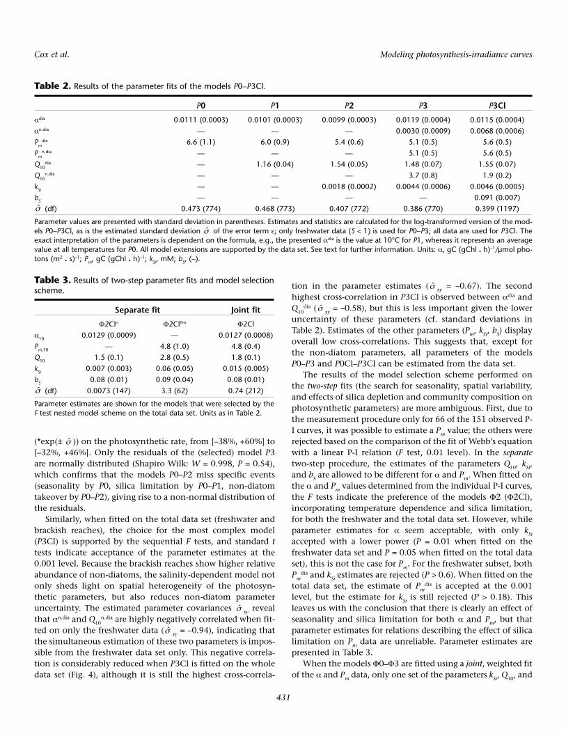
Table 2. Results of the parameter fits of the models P0–P3Cl.

P0 P1 P2 P3 P3Cl

αdia 0.0111 (0.0003) 0.0101 (0.0003) 0.0099 (0.0003) 0.0119 (0.0004) 0.0115 (0.0004)αn.dia — — — 0.0030 (0.0009) 0.0068 (0.0006)Pm

dia 6.6 (1.1) 6.0 (0.9) 5.4 (0.6) 5.1 (0.5) 5.6 (0.5)Pm

n.dia — — — 5.1 (0.5) 5.6 (0.5)Q10

dia — 1.16 (0.04) 1.54 (0.05) 1.48 (0.07) 1.55 (0.07)Q10

n.dia — — — 3.7 (0.8) 1.9 (0.2)kSi — — 0.0018 (0.0002) 0.0044 (0.0006) 0.0046 (0.0005)bS — — — — 0.091 (0.007)

(df) 0.473 (774) 0.468 (773) 0.407 (772) 0.386 (770) 0.399 (1197)

Parameter values are presented with standard deviation in parentheses. Estimates and statistics are calculated for the log-transformed version of the mod-els P0–P3Cl, as is the estimated standard deviation of the error term ε; only freshwater data (S < 1) is used for P0–P3; all data are used for P3Cl. Theexact interpretation of the parameters is dependent on the formula, e.g., the presented αdia is the value at 10°C for P1, whereas it represents an averagevalue at all temperatures for P0. All model extensions are supported by the data set. See text for further information. Units: α, gC (gChl . h)–1/µmol pho-tons (m2 . s)–1; Pm, gC (gChl . h)–1; kSi, mM; bS, (–).

σ̂

σ̂

Table 3. Results of two-step parameter fits and model selectionscheme.

Separate fit Joint fit

Φ2Clα Φ2ClPm Φ2Clα10 0.0129 (0.0009) — 0.0127 (0.0008)Pm,10 — 4.8 (1.0) 4.8 (0.4)Q10 1.5 (0.1) 2.8 (0.5) 1.8 (0.1)kSi 0.007 (0.003) 0.06 (0.05) 0.015 (0.005)bS 0.08 (0.01) 0.09 (0.04) 0.08 (0.01)

(df) 0.0073 (147) 3.3 (62) 0.74 (212)

Parameter estimates are shown for the models that were selected by theF test nested model scheme on the total data set. Units as in Table 2.

σ̂

Cox et al. Modeling photosynthesis-irradiance curves

432

bS and is obtained. In this selection scheme, the model Φ3 isselected when fitted on the freshwater subset, but only Φ2Clwhen fitted on the total data set. Standard t tests indicateacceptance of all parameter estimates at the 0.001 level exceptfor kSi; the estimate of kSi is accepted at the 0.01 level when esti-

mated from the total data set, but is rejected when Φ3 is fittedon the freshwater data set. The obtained parameter estimatesare largely comparable to the estimates of the direct fit, exceptfor the estimate of kSi, which is larger in the two-step fit by afactor of 3. For all parameters, both the variances and cross-cor-

Fig. 4. Estimated covariance matrix of the parameters of the model P3Cl, visualized by plotting the 50% and 90% ellipses of all parameter combina-tions (lower left part). The correlation coefficient of each parameter combination is given in the upper right part.

Cox et al. Modeling photosynthesis-irradiance curves

433

relations are much higher in the two-step fit procedure. In par-ticular, the estimates of kSi and Q10 are highly correlated ( xy =–0.53), and both parameters cannot be estimated simultane-ously from this data set. Both deviate from the direct fit esti-mates by twice their standard deviation, indicating that thiscross-correlation is the cause of the unrealistic parameter esti-mate of kSi, and to a lesser extend Q10 in the two-step approach.The failure to select the most complex model Φ3 (in both theseparate and the joint fits) would suggest no effect of commu-nity composition (diatoms versus non-diatoms) on the photo-synthetic parameters. The acceptance of Φ3 when fitted onlyon the freshwater subset does hint at a possible effect of com-munity composition, but the concomitant rejection of the esti-mate of kSi makes this assertion uncertain.

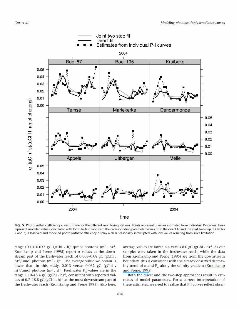
The direct and two-step procedures are further compared intwo ways, namely by their capability to reproduce spatiotem-poral patterns of the photosynthetic parameters on the onehand, and their capability to reproduce observed photosyn-thetic rates on the other. The spatial and temporal patterns ofthe photosynthetic efficiency α and the correspondence withthe selected models are presented in Figs. 5 and 6. For thedirect fit, the derived formulations from P3Cl are used (i.e.,Φ3Cl, similar to Eq. 11), with parameter values obtained in thedirect fit (Table 2). The photosynthetic efficiency (and the cor-responding models) shows a distinct overall spatiotemporalpattern, with a clear seasonality, interfered by the effects of sil-ica limitation and with a downstream increasing trend super-imposed on it. The effect of silica depletion is reflected by theextremely low α values in summer. In 2003, depletion wasrecorded during a single month (August) at several stations inthe freshwater reach (Fig. 2), giving rise to a pronounced min-imum in the α values (Fig. 5). In 2004, the extended period ofsilica depletion (Fig. 2) gave rise to overall lower α, comparedwith 2003 (Fig. 5). Silica depletion also increases the variationof the photosynthetic efficiency along the salinity gradient:the increase with salinity is most pronounced when it is com-plemented with silica depletion in the freshwater reach. Moststriking is the factor-4 difference between maximum and min-imum photosynthetic efficiency in August 2003 and 2004along the estuary axis, correctly reproduced by the models(Fig. 6). The 66 withheld Pm values result in a sparse data set.Therefore, the correspondence between observed and mod-eled spatiotemporal patterns of Pm is not very instructive, andis not shown. By construction, however, the modeled Pm dis-plays the same spatiotemporal features as α (in the case of thejoint fit the modeled Pm is proportional to the modeled α).

Although the model selection scheme and the overallreproduction of spatiotemporal patterns demonstrate rele-vance of the models used and the parameter estimates, regres-sion of the modeled α and Pm against the respective valuesdetermined from the individual P-I curves shows considerablescatter (Fig. 7 B and C). This illustrates that a lot of variabilityin the parameters remains unexplained by the models, likelyowing to the simplicity of the formulations, and partly to nat-

ural variability and introduced measurement errors.In the end, we are not interested in photosynthetic param-

eters only, but also in (the accuracy of) the estimate of photo-synthetic rates. In case of the two-step fits, photosyntheticrates are calculated by substituting the modeled α and Pm inWebb’s equation. This results in a new selection scheme forthe two-step fits, now based on the residuals of the photosyn-thetic rates. As can be read from Table 4, the models selectedin the two-step scheme underperform when used to calculatephotosynthetic rates. The residual error of the selected modelis larger than for the simplest model in the direct fit (P0, i.e.,one curve fitted through all P-I data points; Table 2), and theresiduals of this selected model are larger than the ones fromthe more simple models. As such, while based on the α and Pm

values the models Φ2Cl are selected, they would be rejectedbased on the photosynthetic rate data. In the new selectionscheme, the model Φ1Cl would be preferred for the joint two-step fits, whereas Φ3Cl for α in combination with Φ1Cl for Pm

would be preferred for the separate two-step fits (F test, 0.01level).

Thus, although there is certainly spatiotemporal variationin the photosynthetic parameters that is partly reproduced bythe respective models (cf. Figs. 5 and 6), these formulationsand associated parameter estimates underperform when usedto calculate photosynthetic rates. This reflects the changingshape of the P-I curve under, e.g., silica-depleted conditions:only a Webb-shaped P-I curve is entirely characterized by theinitial slope and the maximal value of this function.

Moreover, when only studying the photosynthetic parame-ters, the above comparison of calculated and observed photo-synthetic rates is normally not possible, as the original P-I dataare needed. The induced residual error, calculated by MonteCarlo simulation based on the residual error of the α and Pm

model fits (Table 3), is distinctly larger than the real residualerror, for both the separate and the joint procedure (Table 4).These results suggest that the two-step procedures, as they areapplied on fewer data points, result in an underestimation ofthe (already poor) predictive capacity of the fitted modelswhen used to calculate photosynthetic rates.

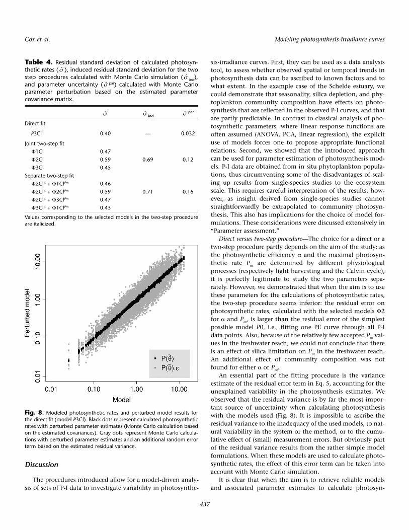
Finally, a Monte Carlo simulation also sheds light on therelative importance of parameter uncertainty and residualuncertainty. Random parameter values are calculated basedon the estimated covariance matrix. The effect of parameteruncertainty on the calculated photosynthetic rates is only 8%of total uncertainty (perturbed parameters + residual error) inthe direct fit (Table 4), demonstrating that model uncertainty(the residual error term) is the main contributor to uncertaintyin photosynthetic rate calculations, even with the model P3Cl(Fig. 8). In the two-step fit procedure, the estimated contribu-tion of parameter uncertainty is higher, but still relativelysmall compared with total uncertainty (Table 4).

Assessment of parameter estimates and model formulations—Asa first step in the two-step fit procedure, α and Pm values areobtained from each P-I curve. Freshwater α values are in the

%θ

σ̂

Cox et al. Modeling photosynthesis-irradiance curves

434

range 0.004–0.037 gC (gChl . h)–1/µmol photons (m2 . s)–1.Kromkamp and Peene (1995) report α values at the down-stream part of the freshwater reach of 0.005–0.08 gC (gChl .h)–1/µmol photons (m2 . s)–1. The average value we obtain islower than in this study, 0.013 versus 0.032 gC (gChl .h)–1/µmol photons (m2 . s)–1. Freshwater Pm values are in therange 1.10–18.4 gC (gChl . h)–1, consistent with reported val-ues of 0.7–18.8 gC (gChl . h)–1 at the most downstream part ofthe freshwater reach (Kromkamp and Peene 1995). Also here,

average values are lower, 4.4 versus 8.0 gC (gChl . h)–1. As oursamples were taken in the freshwater reach, while the datafrom Kromkamp and Peene (1995) are from the downstreamboundary, this is consistent with the already observed decreas-ing trend of α and Pm along the salinity gradient (Kromkampand Peene, 1995).

Both the direct and the two-step approaches result in esti-mates of model parameters. For a correct interpretation ofthese estimates, we need to realize that P-I curves reflect obser-

Fig. 5. Photosynthetic efficiency α versus time for the different monitoring stations. Points represent α values estimated from individual P-I curves. Linesrepresent modeled values, calculated with formula Φ3Cl and with the corresponding parameter values from the direct fit and the joint two-step fit (Tables2 and 3). Observed and modeled photosynthetic efficiency display a clear seasonality interrupted with low values resulting from silica limitation.

Cox et al. Modeling photosynthesis-irradiance curves

435

vations of photosynthesis of a varying phytoplankton com-munity. Therefore, although the model structure is mathe-matically similar to simple models of single-species photosyn-thesis, both model output and parameter estimates should be

interpreted in terms of community photosynthesis. This is themajor difference with other model studies. In particular, Gei-der et al. (1997) used very similar models, but applied them tosingle-species data. Specifically, the observed seasonality is the

Fig. 6. Photosynthetic efficiency α versus distance from the estuary mouth for the different months of sampling. Points represent α values estimatedfrom individual P-I curves. Lines represent modeled values, calculated with formula Φ3Cl and with the corresponding parameter values from the directfit and the joint two-step fit (Tables 2 and 3). Observed and modeled photosynthetic efficiency display a clear downstream increasing trend, becomingmore pronounced when silica is depleted in the freshwater reaches.

Cox et al. Modeling photosynthesis-irradiance curves

436

aggregated result of the succession of phytoplankton species(with associated photosynthetic characteristics) and effects oftemperature on photosynthetic rates. Therefore, the estimatedQ10 parameter is conceptually different from the ones obtainedfrom single-species studies, which represent only effect oftemperature on photosynthesis. Similar remarks can be madeabout the estimated kSi.

This also implies that insights from single-species studieson model structure or physiology should be carefully exam-ined on their meaning and relevance for community photo-synthesis. For instance, there is little temperature dependenceof photosynthetic efficiency of individual species (Coles andJones 2000; Morris and Kromkamp 2003). But this does notmean a priori that a multiplicative temperature dependence ofcommunity photosynthesis (as used above) is inappropriate.On the contrary, the results from our analysis demonstratesthat there is seasonal variability in the α of the communityphotosynthesis.

Concerning the effect of nutrient limitation on communityphotosynthesis, the argument is slightly different. There isempirical evidence that the effect of nitrogen depletion onsingle-species algal growth is not best described by a multi-plicative factor (Flynn 2003a), and this should also hold forcommunity photosynthesis. However, Lippemeier et al. (1999)observed a direct effect of silica limitation on the photosyn-thetic performance of diatoms and assumed a strong influenceof silicate metabolism on the photosynthetic efficiency. Thissupports the choice for a model formulation in which low sil-ica concentrations affect not only Pm but also α. Our analysisconfirms this observation, specifically by the selection of themodel Φ2 for α in the two-step fit procedure. Lower values ofα during periods of silica depletion are also obvious in Figs. 5and 6.

Finally, the parameter covariance, as presented in Fig. 4,should also not be interpreted as if these parameters necessar-ily would co-vary; rather, it indicates whether the differentparameters can be estimated independently in this model fitscheme. A high correlation between two parameters indicatesthis is not the case.

The foregoing remarks notwithstanding, the parameterestimates obtained in the direct fit are realistic, in the sensethat they are comparable to literature values of their physio-logical counterparts. Sobrino and Neale (2007) reported a Q10

value of 1.4 for the growth of the estuarine diatom Thalas-siosira pseudonana over the temperature range 10–20°C, whichis close to the Q10 value from the direct fit (1.48 in freshwater,1.55 for the total data set; Table 2). The half-saturation for sil-ica limitation (kSi) of 4.5 µM is at the higher end of reportedhalf-saturation values for diatom growth, with these highestvalues reported specifically for growth in freshwater environ-ment (Martin-Jezequel et al. 2000). So, although care has to betaken with the interpretation of parameters, their numericalvalues are confined by their physiological counterparts. Thisgives extra support for the nested model procedure.

Fig. 7. Photosynthetic rates calculated with the directly fitted model(P3Cl) versus observed rates (A; note the log scale). Modeled photosyn-thetic efficiency (B) and maximum photosynthetic rate (C), calculatedwith parameter values from the direct fit, versus respective values fromindividual P-I curve fits.

Cox et al. Modeling photosynthesis-irradiance curves

437

Discussion

The procedures introduced allow for a model-driven analy-sis of sets of P-I data to investigate variability in photosynthe-

sis-irradiance curves. First, they can be used as a data analysistool, to assess whether observed spatial or temporal trends inphotosynthesis data can be ascribed to known factors and towhat extent. In the example case of the Schelde estuary, wecould demonstrate that seasonality, silica depletion, and phy-toplankton community composition have effects on photo-synthesis that are reflected in the observed P-I curves, and thatare partly predictable. In contrast to classical analysis of pho-tosynthetic parameters, where linear response functions areoften assumed (ANOVA, PCA, linear regression), the explicituse of models forces one to propose appropriate functionalrelations. Second, we showed that the introduced approachcan be used for parameter estimation of photosynthesis mod-els. P-I data are obtained from in situ phytoplankton popula-tions, thus circumventing some of the disadvantages of scal-ing up results from single-species studies to the ecosystemscale. This requires careful interpretation of the results, how-ever, as insight derived from single-species studies cannotstraightforwardly be extrapolated to community photosyn-thesis. This also has implications for the choice of model for-mulations. These considerations were discussed extensively in“Parameter assessment.”

Direct versus two-step procedure—The choice for a direct or atwo-step procedure partly depends on the aim of the study: asthe photosynthetic efficiency α and the maximal photosyn-thetic rate Pm are determined by different physiologicalprocesses (respectively light harvesting and the Calvin cycle),it is perfectly legitimate to study the two parameters sepa-rately. However, we demonstrated that when the aim is to usethese parameters for the calculations of photosynthetic rates,the two-step procedure seems inferior: the residual error onphotosynthetic rates, calculated with the selected models Φ2for α and Pm, is larger than the residual error of the simplestpossible model P0, i.e., fitting one PE curve through all P-Idata points. Also, because of the relatively few accepted Pm val-ues in the freshwater reach, we could not conclude that thereis an effect of silica limitation on Pm in the freshwater reach.An additional effect of community composition was notfound for either α or Pm.

An essential part of the fitting procedure is the varianceestimate of the residual error term in Eq. 5, accounting for theunexplained variability in the photosynthesis estimates. Weobserved that the residual variance is by far the most impor-tant source of uncertainty when calculating photosynthesiswith the models used (Fig. 8). It is impossible to ascribe theresidual variance to the inadequacy of the used models, to nat-ural variability in the system or the method, or to the cumu-lative effect of (small) measurement errors. But obviously partof the residual variance results from the rather simple modelformulations. When these models are used to calculate photo-synthetic rates, the effect of this error term can be taken intoaccount with Monte Carlo simulation.

It is clear that when the aim is to retrieve reliable modelsand associated parameter estimates to calculate photosyn-

Table 4. Residual standard deviation of calculated photosyn-thetic rates ( ), induced residual standard deviation for the twostep procedures calculated with Monte Carlo simulation ( ind),and parameter uncertainty ( par) calculated with Monte Carloparameter perturbation based on the estimated parametercovariance matrix.

indpar

Direct fit

P3Cl 0.40 — 0.032

Joint two-step fitΦ1Cl 0.47Φ2Cl 0.59 0.69 0.12Φ3Cl 0.45

Separate two-step fitΦ2Clα + Φ1ClPm 0.46Φ2Clα + Φ2ClPm 0.59 0.71 0.16Φ2Clα + Φ3ClPm 0.47Φ3Clα + Φ1ClPm 0.43

Values corresponding to the selected models in the two-step procedureare italicized.

σ̂

σ̂σ̂

σ̂

σ̂

σ̂

Fig. 8. Modeled photosynthetic rates and perturbed model results forthe direct fit (model P3Cl). Black dots represent calculated photosyntheticrates with perturbed parameter estimates (Monte Carlo calculation basedon the estimated covariances). Gray dots represent Monte Carlo calcula-tions with perturbed parameter estimates and an additional random errorterm based on the estimated residual variance.

Cox et al. Modeling photosynthesis-irradiance curves

438

thetic rates, the direct fit approach is more appropriate. More-over, the parameter estimates obtained from the analysis of P-I curves might be more useful for ecosystem models thanparameter values from single-species studies. For example,concerning the Q10 values, in these models it is exactly the sea-sonality (i.e., the aggregate effect of successive phytoplanktonpopulations and the temperature dependence of photosyn-thetic rates) that has to be reproduced, and not specifically thetemperature dependence of photosynthesis.

Of course the usual precautions need to be taken whenusing these parameter estimates for model studies outsidethe study period for which parameters are estimated. Partic-ularly for our study site, considerable changes in phyto-plankton biomass and species composition have beenreported over the last decade (Cox et al. 2009). Possibly thesechanges also affected the community photosynthesis param-eters, their seasonal variation, and their responses to nutri-ent limitation. In such a setting, the parameter estimates andmodel formulations can be considered valid only for thestudy period, unless an additional validation study is per-formed with other data. Besides, in such a validation studythe presented method could prove to be a useful tool. Whena new data set would be available for validation, the meth-ods outlined above could be used to assess whether a modelwith data set–specific photosynthesis parameters fits the datasignificantly better than a model with constant parametersfor the combined data set. Otherwise, when applying themodels and parameter estimates in model simulations forthe 2003–2004 period, it is clear that the parameters as pre-sented give the best “average” model output for the period.Moreover, parameter estimates from the direct fit on the2003 data only are very similar to the estimates obtained inthe fit from 2003–2004. On the other hand, in 2004 the pro-longed period of silica limitation almost completely masksthe seasonality (Fig. 5). When models are fitted on this sub-set, the parameter estimates are unphysical, notably with aQ10 value smaller than 1. This illustrates a general weaknessof the presented method compared with laboratory studies.When different environmental factors interact and poten-tially neutralize each other, success of the method presentedwill partly depend on the access to a good data set, where theeffect of the different factors is separable.

Extension to more complex models—Although the modelstructures we used are fairly standard and widely used (Webbmodel for photosynthetic rate, Monod formulation for silicalimitation, Q10 structure for temperature dependence), theyare empirical mathematical formulations for algal growthand photosynthesis for which more detailed mechanisticmodels have been developed (Flynn 2003b; Baklouti et al.2006). It is possible to generalize the method outlined and fitmore complex models to measured P-I curves. It has beenreported that published data sets (mainly based on labora-tory cultures) are not adequate for rigorous testing of com-plex models (Flynn and Martin-Jezequel 2000), a statement

that was made in the context of the interaction between sil-ica stress and photosynthesis. Our study suggests that elabo-rate sets of (in situ) measured P-I curves, and to a lesserextent sets of α and Pm values determined from individual P-I curves, under varying environmental conditions, could bevaluable data sets for the evaluation of these complex mod-els. Because they aim at a broad applicability, they should atleast be able to reproduce these curves and the photosyn-thetic parameters α and Pm.

Comments and recommendationsFitting models to historical and present P-I data provides a

useful tool to study the role of certain environmental cues onvariation in phytoplankton community photosynthesis. Incontrast to results from laboratory and single-species studies,sets of P-I data reflect the behavior of natural phytoplanktonassemblages. The model-based study of these P-I data providesinsight to the relation between the variability in communityphotosynthesis and environmental covariates. Such studycomplements single-species studies, from which it is notstraightforward to infer characteristics of phytoplanktonassemblages at the ecosystem scale. The parameter estimatesthat can be retrieved from the study of P-I data might be moreuseful in ecosystem models than literature values from singlespecies.

Strikingly, there is a large amount of residual variation notaccounted for by the used model formulations. Obviously, thispartly results from the simplicity of the model formulationsused, although they are common in ecosystem models. Butalso, species composition in the study area is considerablydynamic, and it would be interesting to investigate in moredetail the effect of phytoplankton species succession onassemblage photosynthesis. This could also shed light on theaccurateness of 14C incubation to estimate community photo-synthesis. Information on the origins of variability of com-munity photosynthesis is important to assess the year-to-yearvariability and predictability of ecosystem photosynthesis.

To prevent overfitting of multiparameter models, we haveput forward some statistical tools based on a nested modelselection scheme. Refinement of these tools is probably possi-ble. The quality of the results depend on the quality of thevariety of data sources used (14C incubations, nutrient con-centrations, species composition determination). Therefore,the assessment of the resulting parameter estimates and theevaluation of the model formulation used will benefit fromthe use of more advanced statistics. Probably, also these statis-tics will need to be adapted to the specific situation whenapplied to other systems.

We conclude that a direct fit is to be preferred when theaim is to characterize and reproduce the variability of photo-synthetic rates. The use of P-I data allows for a more powerfulanalysis of community photosynthesis. Therefore it is recom-mended that not only photosynthetic parameters are docu-mented and analyzed, but rather the whole set of P-I data.

Cox et al. Modeling photosynthesis-irradiance curves

439

References

Alpine, A. E., and J. E. Cloern. (1988). Phytoplankton growth-rates in a light-limited environment, San-Francisco Bay.Mar Ecol-Prog Ser. 44:167–173. [doi:10.3354/meps044167].

Baklouti, M., F. Diaz, C. Pinazo, V. Faure, and B. Queguiner.(2006). Investigation of mechanistic formulations depict-ing phytoplankton dynamics for models of marine pelagicecosystems and description of a new model. Prog.Oceanogr. 71:1–33. [doi:10.1016/j.pocean.2006.05.002].

Cole, B. E. (1989). Temporal and spatial patterns of phyto-plankton production in Tomales bay, California, USA.Estuar. Coast. Shelf Sci. 28:103–115. [doi:10.1016/0272-7714(89)90045-0].

Coles, J., and R. Jones. (2000). Effect of temperature on pho-tosynthesis-light response and growth of four phytoplank-ton species isolated from a tidal freshwater river. J. Phycol.36:7–16. [doi:10.1046/j.1529-8817.2000.98219.x].

Cox, T. J. S., T. Maris, K. Soetaert, D. J. Conley, S. Van Damme,P. Meire, J. J. Middelburg, M. Vos, and E. Struyf. (2009). Amacro-tidal freshwater ecosystem recovering from hypereu-trophication: The Schelde case study. Biogeosciences6:2935–2948. [doi:10.5194/bg-6-2935-2009].

Davidson, K., and W. S. C. Gurney. (1999). An investigation ofnon-steady-state algal growth. II. Mathematical modellingof co-nutrient-limited algal growth. J. Plankt. Res.21:839–858. [doi:10.1093/plankt/21.5.839].

Flynn, K. J. (2003a). Do we need complex mechanistic pho-toacclimation models for phytoplankton? Limnol.Oceanogr. 48:2243–2249. [doi:10.4319/lo.2003.48.6.2243].

Flynn, K. J. (2003b). Modelling multi-nutrient interactions inphytoplankton; balancing simplicity and realism. Prog.Oceanogr. 56:249–279. [doi:10.1016/S0079-6611(03)00006-5].

Flynn, K. J., and V. Martin-Jezequel. (2000). Modelling Si-N-limited growth of diatoms. J. Plankt. Res. 22:447–472.[doi:10.1093/plankt/22.3.447].

Gazeau, F., J. P. Gattuso, J. J. Middelburg, N. Brion, L. S. Schi-ettecatte, M. Frankignoulle, and A. V. Borges. (2005). Plank-tonic and whole system metabolism in a nutrient-rich estu-ary (the Scheldt estuary). Estuaries 28:868–883. [doi:10.1007/BF02696016].

Geider, R. J., H. L., MacIntyre, and T. M. Kana. (1997).Dynamic model of phytoplankton growth and acclimation:Responses of the balanced growth rate and the chlorophylla:carbon ratio to light, nutrient-limitation and tempera-ture. Mar. Ecol. Prog. Ser. 148:187–200. [doi:10.3354/meps148187].

Goebel, N. L., and J. N. Kremer. (2007). Temporal and spatialvariability of photosynthetic parameters and communityrespiration in long island sound. Mar. Ecol. Prog. Ser.329:23–42. [doi:10.3354/meps329023].

Goosen, N. K., J. Kromkamp, J. Peene, P. van Rijswijk, and P.van Breugel. (1999). Bacterial and phytoplankton produc-tion in the maximum turbidity zone of three European

estuaries: The Elbe, Westerschelde and Gironde. J. Mar. Syst.22:151–171. [doi:10.1016/S0924-7963(99)00038-X].

Keller, A. A. (1988). An empirical-model of primary productiv-ity (C-14) using mesocosm data along a nutrient gradient.J. Plankt. Res. 10:813–834. [doi:10.1093/plankt/10.4.813].

Kromkamp, J., and J. Peene. (1995). On the possibility of netprimary production in the turbid Schelde estuary (SWNetherlands). Mar. Ecol. Prog. Ser. 121:249–259. [doi:10.3354/meps121249].

Lewitus, A., D. White, R. Tymowski, M. Geesey, S. Hymel, andP. Noble. (2005). Adapting the CHEMTAX method forassessing phytoplankton taxonomic composition in South-eastern U.S. estuaries. Estuaries 28:160–172. [doi:10.1007/BF02732761].

Lionard, M., K. Muylaert, M. Tackx, and W. Vyverman. (2008).Evaluation of the performance of HPLC-CHEMTAX analy-sis for determining phytoplankton biomass and composi-tion in a turbid estuary (Schelde, Belgium). Estuar. Coast.Shelf Sci. 76:809–817. [doi:10.1016/j.ecss.2007.08.003].

Lippemeier, S., P. Hartig, and F. Colijn. (1999). Direct impactof silicate on the photosynthetic performance of thediatom Thalassiosira weissflogii assessed by on- and off-linePAM fluorescence measurements. J. Plankt. Res.21:269–283. [doi:10.1093/plankt/21.2.269].

MacIntyre, H. L., and J. J. Cullen. (1996). Primary productionby suspended and benthic microalgae in a turbid estuary:Time-scales of variability in San Antonio bay, Texas. Mar.Ecol. Prog. Ser. 145:245–268. [doi:10.3354/meps145245].

Mackey, M., D. Mackey, H. Higgins, and S. Wright. (1996).CHEMTAX—a program for estimating class abundance forchemical markers: Application to HPLC measurements ofphytoplankton. Mar. Ecol. Prog. Ser. 144:265–283.[doi:10.3354/meps144265].

Martin-Jezequel, V., M. Hildebrand, and M. A. Brzezinski.(2000). Silicon metabolism in diatoms: Implications forgrowth. J. Phycol. 36:821–840. [doi:10.1046/j.1529-8817.2000.00019.x].

Meire, P., T. Ysebaert, S. Van Damme, E. Van den Bergh, T.Maris, and E. Struyf. (2005). The Scheldt estuary: A descrip-tion of a changing ecosystem. Hydrobiologia 540:1–11.[doi:10.1007/s10750-005-0896-8].

Mizon, G. E. (1977). Inferential procedures in nonlinear mod-els: Application in a UK industrial cross-section study offactor substitution and returns to scale. Econometrica45:1221–1242. [doi:10.2307/1914069].

Morris, E., and J. Kromkamp. (2003). Influence of temperatureon the relationship between oxygen- and fluorescence-based estimates of photosynthetic parameters in a marinebenthic diatom (Cylindrotheca closterium). Eur. J. Phycol.38:133–142. [doi:10.1080/0967026031000085832].

Muylaert, K., K. Sabbe, and W. Vyverman. (2000). Spatial andtemporal dynamics of phytoplankton communities in afreshwater tidal estuary (Schelde, Belgium). Estuar. Coast.Shelf Sci. 50:673–689. [doi:10.1006/ecss.2000.0590].

Press, W. H., S. A. Teukolsky, W. T. Vetterling, and B. P. Flan-nery. (2003). Numerical recipes in Fortran 77: The art of sci-entific computing. Cambridge University Press.

R Development Core Team (2006). R: A language and envi-ronment for statistical computing. R Foundation for Statis-tical Computing, Vienna, Austria. ISBN 3-900051-07-0.

Schlüter, L., F. Møhlenberg, H. Havskum, and S. Larsen.(2000). The use of phytoplankton pigments for identifyingand quantifying phytoplankton groups in coastal areas:Testing the influence of light and nutrients on pig-ment/chlorophyll a ratios. Mar. Ecol. Prog. Ser. 192:49–63.[doi:10.3354/meps192049].

Seber, G., and C. Wild. (1989). Nonlinear regression. Wileyseries in probability and mathematical statistics. Appliedprobability and statistics. John Wiley and Sons.

Sobrino, C., and P. J. Neale. (2007). Short-term and long-termeffects of temperature on photosynthesis in the diatomThalassiosira pseudonana under UVR exposures. J. Phycol.43:426–436. [doi:10.1111/j.1529-8817.2007.00344.x].

Steemann Nielsen, E. (1951). Measurement of the productionof organic matter in the sea by means of carbon-14. Nature167:684–685. [doi:10.1038/167684b0 PMid:14826912].

Strickland, J., and T. Parsons. (1972). A practical handbook ofseawater analyses. Ottawa: Fisheries Research Board of

Canada, 2nd edition.Unesco (1985). The International System of Units (SI) in

Oceanography. Unesco Technical Papers in Marine Science45, Unesco, Paris.

Van Damme, S., E. Struyf, T. Maris, T. Ysebaert, F. Dehairs, M.Tackx, C. Heip, and P. Meire. (2005). Spatial and temporalpatterns of water quality along the estuarine salinity gradi-ent of the Scheldt estuary (Belgium and The Netherlands):Results of an integrated monitoring approach. Hydrobiolo-gia 540:29–45. [doi:10.1007/s10750-004-7102-2].

Webb, W., M. Newton, and D. Starr. (1974). Carbon-dioxideexchange of Alnus-Rubra: Mathematical-model. Oecologia17:281–291. [doi:10.1007/BF00345747].

Wright, S., and S. Jeffrey. (1997). High resolution system forchlorophylls and carotenoids of marine phytoplankton. InS. Jeffrey, R. Mantoura, and S. Wright (Eds.), Phytoplanktonpigments in oceanography: A guide to advanced methods(pp. 327–341). Paris: SCOR-UNESCO.

Yentsch, C., and D. Menzel. (1963). A method for the deter-mination of phytoplankton chlorophyll and phaeophytinby fluorescence. Deep-Sea Res. 221–231.

Submitted 12 January 2010Revised 18 May 2010Accepted 1 July 2010

440

Cox et al. Modeling photosynthesis-irradiance curves