modeling of two stage nozzle-flapper type - METU

MODELING OF TWO STAGE NOZZLE-FLAPPER TYPE

ELECTROHYRAULIC SERVOVALVES

A THESIS SUBMITTED TO

THE GRADUATE SCHOOL OF NATURAL AND APPLIED SCIENCES

OF

MIDDLE EAST TECHNICAL UNIVERSITY

BY

Ahmet Can Afatsun

IN PARTIAL FULFILLMENT OF THE REQUIREMENTS

FOR

THE DEGREE OF Master of Science

IN

Mechanical Engineering

May 2019

Approval of the thesis:

MODELING OF TWO STAGE NOZZLE-FLAPPER TYPE

ELECTROHYRAULIC SERVOVALVES

submitted by Ahmet Can Afatsun in partial fulfillment of the requirements for the

degree of Master of Science in Mechanical Engineering Department, Middle

East Technical University by,

Prof. Dr. Halil Kalıpçılar

Dean, Graduate School of Natural and Applied Sciences

Prof. Dr. M. A. Sahir Arıkan

Head of Department, Mechanical Engineering

Prof. Dr. R. Tuna Balkan

Supervisor, Mechanical Engineering, METU

Examining Committee Members:

Prof. Dr. M. Haluk Aksel

Mechanical Engineering, METU

Prof. Dr. R. Tuna Balkan

Mechanical Engineering, METU

Prof. Dr. Y. Samim Ünlüsoy

Mechanical Engineering, METU

Prof. Dr. Bülent E. Platin

Mechanical Engineering, METU

Assoc. Prof. Dr. S. Çağlar Başlamışlı

Mechanical Engineering, Hacettepe University

Date: 29.05.2019

iv

I hereby declare that all information in this document has been obtained and

presented in accordance with academic rules and ethical conduct. I also declare

that, as required by these rules and conduct, I have fully cited and referenced

all material and results that are not original to this work.

Name, Surname:

Signature:

Ahmet Can Afatsun

v

ABSTRACT

MODELING OF TWO STAGE NOZZLE-FLAPPER TYPE

ELECTROHYRAULIC SERVOVALVES

Afatsun, Ahmet Can

Master of Science, Mechanical Engineering

Supervisor: Prof. Dr. R. Tuna Balkan

May 2019, 130 pages

In this thesis, a detailed mathematical model for a double stage nozzle-flapper type

servovalve is developed focusing on its hydraulics. Such valves must comply with

very strict performance requirements of aerospace and military industries. To meet

these requirements, parts of such a servovalve must be manufactured within the

tolerances as low as a few microns. Considering the servovalve consists of many

parts that influence overall performance, it becomes obvious that the servovalve

must be designed carefully as a system by understanding the effect of deviations of

all parameters related to it. Unfortunately, the relations used to define the behavior

of servovalve hydraulics in the literature have shortcomings around the operating

point. This study is conducted with the intention of fulfilling the need of a simulation

model that offers high accuracy on the entire working range. To create such a model,

several CFD analyses are carried out using the commercial software ANSYS

Fluent®. Available turbulence models’ and wall treatment functions’ performances

are compared with the experimental data to find out which models are most suitable

to conduct such analyses. Results of these numerical analyses are used to develop

more accurate analytical models for both first and second stages. These models are

combined in a system simulation model created by using SimScape® blocks. This

vi

final model is tested with a commercial valve’s parameters, provided by the

manufacturer. The results are accurate comparing to the datasheet values.

Keywords: Servovalve, Nozzle-Flapper Valve, Spool Valve, Flow Through Orifice,

Parameter Optimization

vii

ÖZ

İKİ KADEMELİ NOZUL-KANAT TİPİ ELEKTROHİDROLİK

SERVOVALFLERİN MODELLENMESİ

Afatsun, Ahmet Can

Yüksek Lisans, Makina Mühendisliği

Tez Danışmanı: Prof. Dr. R. Tuna Balkan

Mayıs 2019, 130 sayfa

Elektronik ve hidrolik donanımlar arasında ara yüz oluşturma işlevi olan elektro

hidrolik servovalfler, elektronik tahrikin basitliği ile hidrolik eyleyicilerin yüksek

güç yoğunluğunu bir araya getirirler. Servovalflerin hidrolik preslerden füzelere

kadar oldukça geniş kullanım alanları vardır. Bu tez, üstün dinamik başarımları,

güvenilirlikleri ve küçük boyutları nedeniyle havacılık ve savunma uygulamalarında

tercih edilen çift kademeli nozul-kanat tipi servovalflere yoğunlaşmaktadır. Bu

valflerin havacılık ve savunma alanlarında kullanılan her ürün gibi oldukça katı

başarım gereksinimlerini karşılamaları gerekmektedir. Bu gereksinimlerin

karşılanması için servovalf parçalarının birkaç mikronu geçmeyen geometrik

toleranslar içerisinde üretilmesi gerekir. Servovalfin tüm sistem başarımını etkileyen

birçok parçadan oluştuğu göz önüne alındığında, tasarımın sistemi etkileyen tüm

parametrelerin etkilerini anlayarak dikkatli bir şekilde yapılması gerektiği ortaya

çıkmaktadır. Ne yazık ki, literatürde servovalf hidroliğini tanımlayan denklemler

çalışma noktası çevresinde hatalı sonuçlar vermektedir. Bu tezde, tüm çalışma

bölgesinde yüksek doğrulukta sonuç verecek bir benzetim modeli geliştirilmiştir.

Modeli eniyilemek için ANSYS Fluent® ticari yazılımı ile hesaplamalı akışkan

dinamiği (HAD) çözümlemelerinden faydalanılmıştır. Mevcut türbülans modelleri

ve duvar dibi fonksiyonlarının başarımları, en uygun modelleri saptamak amacıyla

viii

deneysel verilerle karşılaştırılmıştır. Sayısal çözümlemeyle elde edilen sonuçlar

kullanılarak hem birinci hem de ikinci kademe için doğruluğu daha yüksek analitik

modeller türetilmiştir. Bu modeller ile SimScape® blokları kullanılarak tüm sistem

için bir benzetim modeli oluşturulmuştur. Bu model, ticari bir valfin üreticisi

tarafından sağlanan parametreleriyle test edilmiştir. Öngörülen çıktıların katalog

verileriyle tutarlı olduğu görülmüştür.

Anahtar Kelimeler: Servovalf, Nozul-Kanat Valfi, Sürgülü Valf, Orifis Akışı,

Parametre Eniyilemesi

ix

To my family

x

ACKNOWLEDGEMENTS

First, I would like to express my sincere appreciation to my thesis supervisor Prof.

Dr. Tuna BALKAN for his support and guidance throughout my thesis study.

I am grateful for the patience Nergis ÖZKÖSE has shown me throughout my thesis

study. Her support made me move on whenever my motivation deteriorated.

Another big thanks is certainly going to my old friend Ümit YERLİKAYA, who

introduced me to ROKETSAN Inc. in the first place. His friendship has been and

will always be priceless to me.

I am in debt of gratitude to my manager Aslı AKGÖZ BİNGÖL in ROKETSAN Inc.

for her friendly support and advices.

I also owe thanks to my department’s advisor Prof. Dr. Bülent Emre PLATİN who

helped me to compose and refine the scientific reports related to my thesis

throughout the study.

I am also grateful for having my friends Tevfik Ozan FENERCİOĞLU, Hasan

YETGİN and Hasan Baran ÖZMEN, and sharing the same cubical with them in the

workplace for years. Their presence is keeping the happiness in the equation in my

professional life and I sincerely hope our friendship lasts till the end of our lives.

Last and certainly the most, I wish to express my sincere thanks to my father Sedat

AFATSUN, my mother Nursel AFATSUN and my beloved brothers Oğuzhan and

Furkan AFATSUN for the support, joy and peace they have given me all my life.

They are the proof that a family is the most precious thing that a person can have.

xi

TABLE OF CONTENTS

ABSTRACT ................................................................................................................. v

ÖZ ............................................................................................................................ vi

ACKNOWLEDGEMENTS ......................................................................................... x

TABLE OF CONTENTS ........................................................................................... xi

LIST OF TABLES ................................................................................................... xiii

LIST OF FIGURES ................................................................................................. xiv

LIST OF ABBREVIATIONS ................................................................................ xviii

LIST OF SYMBOLS ............................................................................................... xix

CHAPTERS

1. INTRODUCTION ................................................................................................ 1

What is Servovalve? .......................................................................................... 1

Motivation Behind This Study .......................................................................... 6

Objectives of the Thesis .................................................................................... 7

Literature Survey ............................................................................................... 8

Outline of the Thesis ....................................................................................... 13

2. CURRENT STATE OF THE ART OF MODELING DOUBLE STAGE

NOZZLE-FLAPPER SERVOVALVES ................................................................... 15

Overview of Servovalve Physical Model ........................................................ 15

Nozzle-Flapper Valve Model .......................................................................... 16

Spool Valve Model .......................................................................................... 19

Limitations and Assumptions of the Existing Models .................................... 29

3. DEVELOPING MORE ACCURATE FLOW MODELS .................................. 35

xii

Determination of Most Suitable Numerical Models ....................................... 35

Nozzle-Flapper Valve Model .......................................................................... 46

Pressure Sensitivity Analysis ................................................................... 60

Spool Valve Model ......................................................................................... 70

4. COMPLETE DYNAMICAL MODEL OF A DOUBLE STAGE NOZZLE-

FLAPPER SERVOVALVE ...................................................................................... 91

SimScape Model ............................................................................................. 92

Armature Assembly .................................................................................. 92

First Stage ................................................................................................. 93

Second Stage ............................................................................................ 94

Simulation of Moog 31 Series Servovalve ................................................... 100

5. SUMMARY AND CONCLUSIONS ............................................................... 113

Summary ....................................................................................................... 113

Conclusions ................................................................................................... 114

Recommendations for Future Work .............................................................. 115

REFERENCES ........................................................................................................ 117

A. MATLAB Codes .............................................................................................. 123

B. Bending of flexure tube and determination of Lf and Ls .................................. 125

C. Bernoulli Force SimScape Block Source Code ................................................ 127

D. Spool Port SimScape Block Source Code ........................................................ 128

E. Typical Parameters for Moog Series 31 Servovalve ........................................ 129

F. Parameter set used in Moog Series 31 Servovalve simulation ......................... 130

xiii

LIST OF TABLES

Table 2.1 – Some typical servovalve parameters ....................................................... 28

Table 2.2 – Numerical values of parameters in Figure 2.12 ...................................... 30

Table 3.1 – Nominal dimensions of tested fixed orifice geometry ............................ 36

Table 3.2 – Equipments used in fixed orifice tests .................................................... 37

Table 3.3 – Pressure drops according to CFD analysis .............................................. 40

Table 3.4 – Information on the grid used in 2D axisymmetric fixed orifice analyses

.................................................................................................................................... 41

Table 3.5 – Calculation details for 2D axisymmetric fixed orifice analyses ............. 42

Table 3.6 – Flow rate estimation error points of turbulence models ......................... 46

Table 3.7 – Calculation details for nozzle-flapper valve discharge coefficient

analyses ...................................................................................................................... 50

Table 3.8 – First stage full factorial analysis desing variables .................................. 54

Table 3.9 – Calculation details for first stage discharge coefficient analyses ........... 55

Table 3.10 – CD,f and CD,n values calculated in 500 μm ............................................ 57

Table 3.11 – Discharge coefficients used with the models ........................................ 66

Table 3.12 – 𝒙𝟎 estimations of the models ................................................................ 66

Table 3.13 – Final set of discharge coefficients ......................................................... 68

Table 3.14 – 𝒙𝟎 values calculated with equation (3.35) ............................................ 69

Table 3.15 – Calculation details for spool valve discharge coefficient analyses ....... 75

Table 3.16 – Equipment used in spool valve test system ........................................... 87

Table 3.17 – Model’s prediction of valve dimensions ............................................... 88

Table 4.1 – Converted parameters ........................................................................... 103

Table 4.2 – Updated parameters .............................................................................. 105

Table C.1 – Typical parameters for Moog Series 31 Servovalve in SI units ........... 129

xiv

LIST OF FIGURES

Figure 1.1 – A simple sketch of a spool valve and its load ......................................... 1

Figure 1.2 – Moog D634-P series single stage servovalve [2] .................................... 3

Figure 1.3 – Cross section view of a double stage nozzle-flapper servovalve [4] ...... 4

Figure 1.4 – Direction of hydraulic component design [17] ....................................... 7

Figure 2.1 – Block diagram representation of double stage servovalve physical

model ......................................................................................................................... 15

Figure 2.2 – Parts of a double stage nozzle-flapper servovalve [5] ........................... 16

Figure 2.3 – Geometric dimensions of a nozzle-flapper valve .................................. 18

Figure 2.4 – Exaggerated view of first stage when both spool and flapper is moved

[9] ............................................................................................................................... 20

Figure 2.5 – Bernoulli force on the spool .................................................................. 21

Figure 2.6 – CAD model of a servovalve sleeve ....................................................... 23

Figure 2.7 – Open and closed conditions of a spool valve control port .................... 24

Figure 2.8 – Eccentricity in closed condition ............................................................ 25

Figure 2.9 – Zero lapped control ports ...................................................................... 26

Figure 2.10 – Spool valve in open position ............................................................... 26

Figure 2.11 – Flow rate vs. curtain length graph of a single nozzle-flapper valve ... 29

Figure 2.12 – Sample nozzle-flapper valve analysis geometry ................................. 30

Figure 2.13 – Flapper force vs. curtain length graph of a single nozzle-flapper valve

................................................................................................................................... 31

Figure 2.14 – Flow rate estimation performances of equations (2.27) and (2.28) .... 32

Figure 2.15 – Comparison of flow rate estimation performances of Anderson’s

algorithm and CFD analysis ...................................................................................... 33

Figure 3.1 – Fixed orifice geometry used in tests and analyses ................................ 35

Figure 3.2 – Isometric view of fixed orifice CAD model cross section .................... 36

Figure 3.3 – Cross sectional view of fixed orifice test assembly .............................. 37

Figure 3.4 – Flow rate vs. pressure drop curve of the tested fixed orifice ................ 38

xv

Figure 3.5 – Cross sectional view from the CAD model of the test assembly .......... 39

Figure 3.6 – Fluid volume used in 3D fixed orifice analysis ..................................... 40

Figure 3.7 – The grid used in 2D axisymmetric fixed orifice analyses ..................... 41

Figure 3.8 – Analysis results with Enhanced Wall Treatment ................................... 43

Figure 3.9 – Analysis results with Menter-Lechner ................................................... 44

Figure 3.10 – Analysis results with Scalable Wall Functions .................................... 45

Figure 3.11 – Two orifices in a nozzle-flapper valve ................................................ 47

Figure 3.12 – Equivalent circuit diagram of a nozzle-flapper valve .......................... 47

Figure 3.13 – Nozzle-flapper valve geometry with only the variable orifice ............ 48

Figure 3.14 – CD,v vs. Re* curve ................................................................................ 50

Figure 3.15 – The effect of bevel angle on CDV for α = 10 and 20° .......................... 52

Figure 3.16 - The effect of bevel angle on CDV for α = 45 and 75° ........................... 53

Figure 3.17 – CDV curve for α = 50° ........................................................................... 54

Figure 3.18 – Fixed orifice and nozzle connected in serial when the flapper is far

away ........................................................................................................................... 56

Figure 3.19 – Flow rate estimation performance of analytical model compared to

CFD data of selected cases ......................................................................................... 58

Figure 3.20 – Control pressure estimation performance of analytical model

compared to CFD data of selected cases .................................................................... 59

Figure 3.21 – First stage models compared in this section ........................................ 61

Figure 3.22 – First stage pressure sensitivity analysis results .................................... 67

Figure 3.23 – Comparison of 𝒙𝟎 values found with or without 𝑷𝒆........................... 70

Figure 3.24 – The truncated conical area between the spool and the sleeve ............. 71

Figure 3.25 – Details of analysis domain ................................................................... 75

Figure 3.26 – Details around the radial clearance in a sample grid ........................... 76

Figure 3.27 – Comparison of discharge coefficient versus Reynolds number

estimation curves obtained using different turbulence model and wall function

combinations .............................................................................................................. 77

xvi

Figure 3.28 – Comparison of discharge coefficient data in the paper of Posa et al. to

the ones obtained by SST k–ω turbulence model. Different discharge coefficients for

same port openings are obtained by using different flow rates. ................................ 78

Figure 3.29 – Comparison of discharge coefficient data obtained by SST k–ω

turbulence model and output of the fitted function ................................................... 79

Figure 3.30 – Parameters which are used to define the underlap condition .............. 80

Figure 3.31 – 𝑪𝜽 curves obtained from CFD analyses .............................................. 80

Figure 3.32 – Change in 𝑪𝜽 with respect to 𝜽 for 𝑹𝒆 ∗< 𝟏𝟎 ................................... 81

Figure 3.33 – Comparison of developed 𝑪𝜽 function to CFD data ........................... 82

Figure 3.34 – The valve geometry which is used to test final model ........................ 83

Figure 3.35 – Flow rate estimations of developed model and CFD analysis ............ 84

Figure 3.36 – Error map of the model’s output for the test case ............................... 85

Figure 3.37 – A picture of the spool and the sleeve used in the tests ........................ 86

Figure 3.38 – Cross-sectional view of tested spool valve’s computer aided design

model ......................................................................................................................... 86

Figure 3.39 – Hydraulic scheme of test configuration .............................................. 87

Figure 3.40 – Comparison of model’s leakage flow rate estimation to test data ....... 89

Figure 3.41 – Comparison of model’s load pressure estimation to test data ............. 89

Figure 4.1 – Outline of the SimScape Model ............................................................ 91

Figure 4.2 – Details of Armature Assembly Component .......................................... 92

Figure 4.3 – Details of First Stage Component ......................................................... 94

Figure 4.4 – Details of Second Stage Component ..................................................... 95

Figure 4.5 – Relation between the control pressure and no-load flow rate ............... 96

Figure 4.6 – Custom spool port block user interface ................................................. 98

Figure 4.7 – No-Load Flow test configuration hydraulic scheme ............................. 99

Figure 4.8 – Cross sectional view of Moog Series 31 Servovalve [4] .................... 101

Figure 4.9 – The locations of the points of which the distances are found ............. 102

Figure 4.10 – Results of the measurement............................................................... 102

Figure 4.11 – Spool position and control flow rate graphs with initial parameter set

................................................................................................................................. 104

xvii

Figure 4.12 – The model suggested in Moog Type 30 Servovales catalogue [5] .... 105

Figure 4.13 - Spool position and control flow rate graphs with updated parameter set

.................................................................................................................................. 106

Figure 4.14 – Bode plot prediction with the updated parameters ............................ 107

Figure 4.15 – Predicted no-load flow curve of Moog Series 31 Servovalve ........... 108

Figure 4.16 – Predicted load pressure curve of Moog Series 31 Servovalve .......... 108

Figure 4.17 - Predicted spool leakage curve of Moog Series 31 Servovalve .......... 109

Figure 4.18 – No-load flow curve with 5 μm overlapped metering ports ................ 109

Figure 4.19 – Load pressure curve with 5 μm overlapped metering ports .............. 110

Figure 4.20 – Spool leakage curve with 5 μm overlapped metering ports .............. 110

Figure 4.21 – No-load flow curve with 5 μm underlapped metering ports .............. 111

Figure 4.22 – Load pressure curve with 5 μm underlapped metering ports ............ 112

Figure 4.23 – Spool leakage curve with 5 μm underlapped metering ports ............ 112

Figure A.1 – Flexure tube and flapper ..................................................................... 125

Figure C.1 – Dimension of Moog Series 31 Servovalve [4] .................................... 129

xviii

LIST OF ABBREVIATIONS

AT : Chamber A to return port

BT : Chamber B to return port

CFD : Computational Fluid Dynamics

FS : Full stroke

PA : Pressure supply to Chamber A port

PB : Pressure supply to Chamber B port

RANS : Reynolds Averaged Navier Stokes

RNG : Renormalization Group

w/ : With

w/o : Without

xix

LIST OF SYMBOLS

𝐴 : Any area [m2]

𝐴𝑓 : Fixed orifice area [m2]

𝐴𝑖𝑛 : Inlet area of a control volume [m2]

𝐴𝑛 : Nozzle area [m2]

𝐴𝑠 : Spool end area [m2]

𝐴𝑜𝑢𝑡 : Outlet area of a control volume [m2]

𝐵 : Radial clearance between a spool and its sleeve [m2]

𝑐𝑐 : The damping coefficient obtained when 𝐹𝑐 is linearized with respect to

𝑥�̇� [N∙m/(m/s)]

𝐶𝐷 : Any discharge coefficient

𝐶𝐷,0 : Discharge coefficient of a critical lapped spool port

𝐶𝐷,𝑒 : Discharge coefficient of the exit orifice

𝐶𝐷,𝑓 : Discharge coefficient of the fixed orifice

𝐶𝐷,𝑛 : Discharge coefficient of the nozzle’s fixed orifice part

𝐶𝐷,𝑠 : Discharge coefficient of an underlapped spool port

𝐶𝐷,𝑣 : Discharge coefficient of the nozzle’s variable orifice part

𝐶𝜃 : Underlapped spool port discharge coefficient correction term

𝑐𝐹𝑆 : Overall damping on first stage [N∙m∙s]

𝑐𝑛 : The damping coefficient obtained when 𝑇𝑛 is linearized with respect to

𝑥�̇� [N∙m/(m/s)]

xx

𝑐𝑠 : Spool damping [N/(m/s)]

𝑐𝑆𝑆 : Overall damping on the second stage [N/(m/s)]

𝐷 : Any diameter [m]

𝐷𝑐 : Curtain diameter [m]

𝐷𝑒 : Exit orifice diameter [m]

𝐷𝑓 : Fixed orifice diameter [m]

𝐷𝑛 : Nozzle diameter [m]

𝐷𝑠 : Spool diameter [m]

𝑒 : Eccentricity between a spool and its sleeve [m]

𝐹𝐵 : Bernoulli force on the spool [N]

𝐹𝑐 : Control force [N]

𝐹𝑙 : Force applied on the flapper by the fluid jet from the left first stage

branch nozzle [N]

𝐹𝑟 : Force applied on the flapper by the fluid jet from the right first stage

branch nozzle [N]

𝐹𝑥 : The fluid force on the spool on the axial direction [N]

𝑖̂ : Unit vector in the axial direction

𝐽 : Total error calculated by the penalty function

𝐽𝐹𝑆 : Inertia of the first stage [N∙m∙s2]

𝑘𝐵 : Bernoulli force spring coefficient [N/m]

𝐾𝐵 : Bernoulli force constant

𝑘𝑐 : The spring coefficient obtained when 𝐹𝑐 is linearized with respect to 𝑥𝑓

[N/m]

xxi

𝑘𝑓𝑏 : Stiffness of the feedback spring [N/m]

𝑘𝑓𝑡 : Stiffness of the flexure tube [N∙m/rad]

𝑘𝑛 : The spring coefficient obtained when 𝑇𝑛 is linearized with respect to 𝜃

[N∙m/rad]

𝐾𝑝𝑠 : Pressure sensitivity [Pa/m]

𝑘𝑇 : Torque constant of the torque motor [N∙m/mA]

𝐿 : Any length [m]

𝐿𝐴𝑇 : Lap length of port AT [m]

𝐿𝐵𝑇 : Lap length of port BT [m]

𝐿𝑐 : Lap length of a nozzle [m]

𝐿𝑑 : Damping length of the spool [m]

𝐿𝑒 : Spool port opening [m]

𝐿𝑒𝑓 : Exit length of a fixed orifice [m]

𝐿𝑒𝑛 : Exit length of a nozzle [m]

𝐿𝑓 : Distance from flapper pivot point to nozzle axis [m]

𝐿𝑃𝐴 : Lap length of port PA [m]

𝐿𝑃𝐵 : Lap length of port PB [m]

𝐿𝑠 : Distance from flapper pivot point to the point where the feedback

spring touches the spool [m]

𝐿𝑡 : Transition length in Anderson’s spool orifice model [m]

𝑀 : Overlapped spool port flow rate formula correction term

𝑚𝑠 : Spool mass [kg]

xxii

�̂�𝑖𝑛 : Unit vector normal to the inlet of a control volume

�̂�𝑜𝑢𝑡 : Unit vector normal to the outlet of a control volume

𝑃𝐴 : Pressure at Chamber A [Pa]

𝑃𝐵 : Pressure at Chamber B [Pa]

𝑃𝑐 : Control pressure (pressure difference between the ends of the spool)

[Pa]

𝑃𝑒 : Exit pressure [Pa]

𝑃𝑖 : Intermediate pressure when a nozzle and a fixed orifice are connected

in serial [Pa]

𝑃𝑖𝑛 : Pressure at the upstream of an orifice [Pa]

𝑃𝑙 : Pressure on the left first stage branch [Pa]

𝑃𝐿 : Load pressure [Pa]

𝑃𝑜𝑢𝑡 : Pressure at the downstream of an orifice [Pa]

𝑃𝑟 : Pressure on the right first stage branch [Pa]

𝑃𝑠 : Supply pressure [Pa]

𝑃𝑇 : Return (tank) pressure [Pa]

�̂� : Unit vector in the radial direction

𝑅 : Any radius [m]

�⃗� : Force exerted on the control volume by its walls [N]

𝑅𝑠 : Spool radius [m]

𝑅𝑥 : Force exerted on the control volume by its walls on the axial direction

[N]

xxiii

𝑅𝑒 : Reynolds number

𝑅𝑒∗ : Estimated Reynolds number

𝑅�̃� : log(𝑅𝑒∗ + 1)

𝑄 : Any flow rate [m3/s]

𝑄𝐴𝑇 : Flow rate from Chamber A to return [m3/s]

𝑄𝐵𝑇 : Flow rate from Chamber B to return [m3/s]

𝑄𝑙 : Flow rate of the fluid jet from the nozzle on left first stage branch

[m3/s] 𝑄𝐿 : Load flow rate [m3/s]

𝑄𝑂𝐿 : Flow rate through an overlapped orifice [m3/s]

𝑄𝑃𝐴 : Flow rate from pressure supply to Chamber A [m3/s]

𝑄𝑃𝐵 : Flow rate from pressure supply to Chamber B [m3/s]

𝑄𝑟 : Flow rate of the fluid jet from the nozzle on right first stage branch

[m3/s] 𝑄𝑈𝐿 : Flow rate through an underlapped orifice [m3/s]

𝑇𝑛 : Torque on the armature assembly applied by the fluid jets from the

nozzles [N·m]

𝑇𝑡𝑚 : Torque applied by the torque motor [N·m]

𝑢𝑙 : Velocity of the fluid jet from the nozzle on left first stage branch [m/s]

𝑢𝑟 : Velocity of the fluid jet from the nozzle on right first stage branch

[m/s] 𝑉 : Any velocity [m/s]

�⃗� 𝑖𝑛 : Velocity vector at the inlet of a control volume [m/s]

�⃗� 𝑜𝑢𝑡 : Velocity vector at the outlet of a control volume [m/s]

𝑤 : Spool port gradient [m]

xxiv

𝑥 : Curtain length [m]

𝑥0 : Curtain length when the flapper is at null position [m]

�̃�0 : The curtain length that makes the pressure sensitivity maximum [m]

𝑥𝑓 : Flapper position at nozzle axis [m]

𝑥�̇� : Flapper velocity at nozzle axis [m/s]

𝑥�̈� : Flapper acceleration at nozzle axis [m/s2]

𝑥𝑠 : Spool position [m]

𝑥�̇� : Spool velocity [m/s]

𝑥�̈� : Spool acceleration [m/s2]

𝛼 : Bevel angle (outer conical angle) of a nozzle [°]

𝛽 : Inner conical of a nozzle [°]

Δ𝑃 : Pressure drop between two points [Pa]

𝜃 : Spool port opening angle [rad]

𝜃𝑓 : Rotational position of the flapper [rad]

𝜃�̇� : Rotational velocity of the flapper [rad/s]

𝜃�̈� : Rotational acceleration of the flapper [rad/s2]

𝜇 : Dynamic viscosity of the working fluid [kg/(m·s)]

𝜌 : Mass density of the working fluid [kg/m3]

1

CHAPTER 1

1. INTRODUCTION

What is Servovalve?

The term “servovalve”, is apparently made up of two separate words: servo and

valve. “Servo”, or in the long form “servomechanism” means an automatic feedback

control system in which the output is mechanical position or one of its derivatives,

while “valve” is the common name for devices which are used to control the flow of

fluids [1]. By using a servovalve, the flow is controlled by controlling the position of

a moving body in the valve. In certain classes of valves, like check valves or

solenoid on/off valves, the purpose is to allow the fluid to flow or not, but the flow

rate is not controlled. In servovalves, the purpose is to control the flow rate precisely

and bidirectionally. A simple sketch of a spool valve, which is the main component

of proportional valves (i.e., single stage servovalves), is given in Figure 1.1 to

illustrate how the flow rate is controlled.

Figure 1.1 – A simple sketch of a spool valve and its load

2

The valve shown in Figure 1.1 is basically a 4-way spool valve. The moving body of

the valve is called “spool”, and the part in which the spool moves, and which

contains ports to direct the fluid to right direction is called “bushing” or “sleeve”.

There are four metering ports on the sleeve, two of which, namely source ports, open

the pressure source (i.e., high-pressure line) to valve chambers and the other two,

namely return ports, open the valve chambers to reservoir/tank (i.e., low-pressure

line). In Figure 1.1, source ports are named as PA and PB each of which opens

pressure source to chamber A and B, respectively. Similarly, the return ports are

named as AT and BT, which open the valve chambers A and B to tank, respectively.

This naming convention is used for metering ports throughout the thesis.

As the spool moves to +x1 direction, PA is opened, and AT is closed. So, chamber A

is opened to high pressure line to increase the chamber pressure p1. On the other

hand, PB is closed and BT is opened too. Obviously, this opens chamber B to low

pressure line to decrease the chamber pressure B. As a result, a pressure difference

between the two sides of the load occurs, which causes a net force to happen on the

load towards +x2 direction. The resulting force moves the load, but movement speed

is limited by the flow rate through the metering ports. This means that by controlling

the openings of the ports, i.e., the position of the spool, the velocity of load is

controlled with the configuration shown in Figure 1.1.

If the spool is moved towards –x1, the ports which are closed before open, chambers

A and B are opened to low- and high-pressure lines, respectively, and the force on

the load occurs in the –x2 direction. So, the motion of the load is controlled

bidirectionally by moving the spool to different directions.

In practical proportional valves, one end of spool is connected to an actuator, which

is usually a force motor or a proportional solenoid. Electronically actuated valves

benefit from the advantages of both electronics (easier signal generation and

transmission) and hydraulics (high power to weight ratio). That is why the

servovalves are referred to with the adjective “electrohydraulic”. The other end of

3

the spool is connected to a position transducer. This way a closed loop system is

obtained to control the position of the spool.

Figure 1.2 – Moog D634-P series single stage servovalve [2]

A commercial example to proportional valves, produced by the company Moog, is

given in Figure 1.2. It has a linear force motor as actuator, a position transducer and

integrated electronic to close the position control loop of the spool and provide

proper input signal to actuator.

The actuator of a single stage servovalve must be chosen so it is strong enough to

overcome the “Bernoulli force” which is caused by the flowing fluid through the

ports of the valve and defined by the equation (1.1) [2] [8];

𝐹 = 𝜌𝑄𝑉 cos69° (1.1)

where 𝜌, 𝑄 and 𝑉 are fluid density, volumetric flow rate and flow velocity at the

metering port, respectively, while the “69º” is the angle with which the flow leaves

the metering port for rectangular port configuration [8] (More on derivation of the

Bernoulli force can be found in Section 2.3). Note that equation (1.1) gives the force

in only one valve chamber. Since a 4-way spool valve has two chambers, the

4

resulting axial force on a servovalve spool is twice of that. Obviously, the more rated

flow a valve has, the greater the Bernoulli force it is subjected to. So, its actuator

must be stronger (i.e., larger in size) to overcome this force. When the actuator is

larger, it draws more current, so the battery or power supply must be larger too. That

is also the case for all the integrated electronics which are used to control the

actuator.

For mobile applications, such as military or aerospace applications, size may matter

a lot. Apart from space limitations, bigger components mean higher mass and

inductance, i.e., worse dynamic performance. The remedy, which was found for

these problems, is to use a pilot stage between the actuator and main stage (i.e., the

spool valve) to amplify the power available to move the spool. The valve created this

way is called a “double stage servovalve”.

Figure 1.3 – Cross section view of a double stage nozzle-flapper servovalve [4]

Figure 1.3 shows a schematic view of a typical double stage nozzle-flapper

servovalve. Its operating principle is as follows;

Pl PrA B

First (Pilot) Stage

Second (Main) Stage

Actuator (Torque Motor)

5

When current is applied to the torque motor, it rotates the armature due to the

magnetic field, let’s say counterclockwise in Figure 1.3. This rotation makes the

flapper to restrict the fluid flow from the nozzle at the right side of the figure, which

causes the pressure “Pr” to increase and “Pl” to decrease. The pressure difference

between two outer faces of the spool causes it to translate to left. So, the valve

chamber A is opened to pressure port, and B is opened to the reservoir. Thus, the

fluid can flow from the pressure source to chamber A, then to chamber B, and then

return to reservoir. As the spool moves, it causes the cantilever feedback spring to

bend, resulting in a torque on the flapper in the opposite direction to the one applied

by the torque motor. This restoring torque retracts the flapper towards its original

position until Pr and Pl are the same, i.e., there is no pressure difference between the

outer faces of spool. At that point spool stops and a flow rate proportional to the

input current is obtained. By changing the sign of the current input, the spool can be

moved in opposite direction, making bidirectional flow control possible.

The purpose of the nozzle-flapper valve as the first stage is to amplify the power

available to control the flow through the second (main) stage. The electrical input

power, which is at an order of magnitude of 0.1 W, is amplified 100 times to 10 W at

the first stage. It is then amplified again at the main stage to around 10 kW of

hydraulic output power [3]. So it works similar to relays in electronic circuits,

controlling a high power with a low power input.

Although the main stage of a servovalve is always a spool valve, the pilot stage may

be jet-pipe valve [4], nozzle-flapper valve [5] or again spool valve [6] especially in

three stage servovalves which amplifies the power output a further 100 times,

compared to two stage servovalves. Among these alternatives, study in this thesis

focuses on double stage nozzle-flapper mechanical feedback servovalves, since it is

the most common type in aerospace applications.

This section as an introduction to the thesis is included to give brief background

information to reader on servovalves. For further information on basics of

6

servovalves one may refer to numerous resources in literature, such as the textbooks

given in [2], [7] and [8].

Motivation Behind This Study

After the first patent was granted for a two stage servovalve in 1949 [9], servovalve

technology matured quickly. Several patents for different designs were granted

between late 50’s and early 60’s (e.g. pressure feedback servovalve [10], [11] and

flow rate feedback servovalve [12]). Among these the patent for a mechanical

feedback flow control double stage servovalve utilizing a double nozzle-flapper

valve for piloting was granted in 1962 [13], which would soon become a de facto

standard for aerospace and military applications.

After late 60’s, the main structure of double stage servovalves remained unchanged.

It was only the developments in smart materials in 2000’s that led to the attempts to

change the electronic portion (i.e., actuator) of electrohydraulic servovalves.

Piezoelectric [14] and magnetostrictive [15] materials seemed as a potential

replacement to torque motor as the valve’s actuator due to their superior dynamic

performance. But the high hysteresis characteristic of smart materials (~%20) makes

them unusable in high precision position control systems. For the hydraulic portion,

every component stays the way they were in Moog’s patent in 1962.

With this maturity in the field, leading companies in the market established their

standard commercial servovalve models and customers must select one from their

catalogues with a little room for customization. But due to increasing performance

requirements especially in military field, custom tailored products are becoming

more and more appealing. As the founder of Alibaba.com, Jack Ma said in a

conference, “world is shifting from standardization to personalization” [16].

7

Figure 1.4 – Direction of hydraulic component design [17]

Figure 1.4 is taken from an article on innovations for hydraulic pumps, but it applies

to valves as well. As it is implied in the figure, developments in numerical

computation models made much faster research and design possible. Although

multi-domain analyses are not used for this study, numerical computations are

utilized to update all the flow equations to get more accurate models. The main aim

is to achieve an accurate overall servovalve model by combining the models for each

component. This model will take the effects of a wide range of parameters on

servovalve performance into account, like the variations in geometric dimensions or

fluid properties, making it possible to design custom servovalves rapidly.

Objectives of the Thesis

A double stage servovalve consists of three sub-components;

1. An actuator to drive the valve – typically a torque motor

8

2. A piloting (first) stage to amplify the power available to control the main

flow – a nozzle-flapper valve in this study

3. The main (second) stage to direct the main flow and control its flow rate –

i.e., a spool valve

In this thesis only the hydraulic aspects of a servovalve will be studied, i.e., only the

first and second stages are the main subjects of this thesis. The actuator will not be

studied.

At first, a deeper understanding on the servovalves will be gained by examining the

existing analytical relations and CFD analyses. Then a complete servovalve model

will be created after verification of results obtained using CFD analyses. Finally, a

case study will be conducted using this model, by interpreting the overall

requirements on a servovalve, determining the requirements on each sub-component

and making a tolerance analysis for geometric dimensions according to the particular

requirements.

Literature Survey

Since servovalve designs were matured back in 60’s and basic relations defining

their performance are well established, textbooks on fluid power control usually

dedicate at least a chapter to them. So, the natural starting point to learn about

servovalves is these textbooks.

Among these textbooks, one particular book is considered as the holy book of fluid

power control and frequently referred to in publications on this field, namely

Hydraulic Control Systems by Herbert Merritt, published in 1967 [7]. Both nozzle-

flapper and spool valves are examined in the book separately and all the basic

equations which define their characteristics are given. Especially the sections on

spool valves give extensive information on characteristics of spool valves, studying

the forces they are exposed to and the effects of geometry on their performance.

9

There is also an informative chapter dedicated to servovalves where both static and

dynamic performances of servovalves were discussed.

Another important reference is the book Fluid Power Control by Blackburn, Reethof

and Shearer published back in 1960 [2], to which Merritt himself refers to in

Hydraulic Control Systems. There are heavy discussions on control valve

configurations and their performance characteristics in this book too. There is also a

chapter on electrohydraulic actuation which discusses two stage servovalves, but

since servovalves still had some way to go in 1960, the information here is not as

mature as it is in ref. [7].

The book by W. Anderson, Controlling Electrohydraulic Systems (1988) is another

notable reference [18]. The basics of spool and nozzle-flapper valves are discussed

again but the book is more involved with application of control theory on fluid

power control.

A more recent textbook on the field is Fluid Power Engineering by M. Rabie,

published in 2009 [19]. There is a whole chapter dedicated on modeling and

simulation of electrohydraulic systems, which is of interest to this thesis.

The second textbook reference from 2009 is the book by J. Watton, Fundamentals of

Fluid Power Control. The basic discussions appear here again but focus is more on

system dynamics and application of the simulation models.

Apart from textbooks, there are also very useful research and conference papers in

literature on modeling of servovalves. A series of papers published in 1988-89

written by J. Lin and A. Akers studied nozzle-flapper modeling and dynamics.

Authors tried to predict both static and dynamic performance of a nozzle-flapper

valve in the first of these papers, using a linear model [20]. The results were

compared to experiments, as well as to the older predictions given in [7] and [21].

The same study was issued again later as a journal paper [22]. Then the authors

10

performed the same analysis using nonlinear models in [23] and obtained similar

results to [20] and [22].

Aung et al. investigated nozzle-flapper valves in terms of flow forces and energy

loss characteristics [24]. CFD analyses were made on different structures and null

clearances. Results for energy loss were compared against experimental results.

Results for flow force proved that the traditional flow force models are valid

especially for smaller null clearances than one tenth of nozzle diameter.

Zhu and Fei proposed a new criterion for designing a nozzle-flapper valve [25].

Traditional design criterion was criticized since its only objective is to maximize the

null control pressure. New performance characteristics for nozzle-flapper valve were

defined in the paper, namely symmetry, linearity and sensitivity of control pressure,

and the new design was made by improving symmetry and linearity but deteriorating

sensitivity. The work is built upon the existing flow models for nozzle-flapper

valves, new performance characteristics were defined by manipulating the existing

mathematical relations and no CFD analyses or experiments were conducted.

Li et al. deduced mathematical models for flow force and forced vibration [26]. The

models were validated with both CFD analyses and experiments. Natural frequency

of armature assembly was measured and effects of inlet pressure fluctuation near that

frequency were investigated. The work is beneficial for understanding the forces on

flapper and behavior of nozzle-flapper valves under these forces.

Kılıç et al. studied the effects of increasing the pressure at nozzle outlet by

introducing a drain orifice before the flow is directed to reservoir after leaving the

nozzle [27]. Existing mathematical relations were used to model the flows. The cases

in which the outlet orifice present or not were compared in dimensionless load

pressure vs. load flow rate graphs. Results showed that by presenting a drain orifice,

variations in load pressure decreases as the load flow rate changes. A similar

analysis on drain orifice was also done by Watton previously [28].

11

Like the papers written on nozzle-flapper valves by Lin and Akers, A. Ellman et al.

have written a series of papers on modeling of spool valves. In [29] and [30], flow in

a short annulus, which is encountered in closed ports of spool valves, and leakage

flow of servovalves were modeled, respectively. In these works, flow models consist

of constants which must be identified according to the characteristic flow and

pressure curves of the valve that is to be modeled. This means that models developed

in these works can only be used to model an existing valve, for the purpose of

predict its performance or design a controller for it. In [31] pressure gain

characteristic of servovalves is studied. Again, a flow model for spool valve ports

which is based on system identification was used. Study of relation between the

pressure gain and internal leakage and influence of internal leakage on system

damping in the work are particularly useful.

Eryılmaz and Wilson conducted a similar work on modeling of servovalves [32].

Their model also relies on predetermined valve data. Model’s parameters must be

identified according to this data, so the purpose is to model an existing valve for

control purposes rather than designing it. Although the model is valid for entire

spool position range, it is not valid for the valves which are not zero lapped.

Another work to include leakage flow in servovalve model for control purposes was

accomplished by Feki and Richard [33]. The study is very similar to Eryılmaz and

Wilsons’s [32], even the experimental data to test the model’s performance was

provided by Dr. Eryılmaz. Their model also deals with zero lapped valves and all

ports must be symmetrical, but they underlined that the model can be extended to

other lapping conditions.

Mookherjee et al. published a valuable study on design of direct drive valves (DDV)

[34]. In the paper, a model for the flows through spool valve control ports was

developed based on analytical relations and boundary layer analysis. Since they

approached the subject from a design point of view, the model’s parameters are all

physical quantities. It can handle a spool valve design with different lapping

12

conditions for all ports and is valid for entire spool position range. Hence the model

can be used for tolerance analysis of geometric dimensions of a spool valve.

In [35] and [36] Gordic et al. modeled a double stage servovalve and studied the

leakage flow in spool valves, respectively. In these works, they based their spool

valve flow model on the study given in [34]. But as opposed to [34], they used a

constant discharge coefficient in their model. They estimated a valve’s load pressure

and internal leakage with respect to spool position using their model and compared

the results to experiments and output of other models from [31] and [32]. Estimation

performance of the model seems reasonable, but the implicit equations making up

the model make it difficult to use it in transient simulations.

Nakada and Ikebe measured the unsteady axial flow force on spool valve and

compared the result to the theoretical model [37]. The theoretical model that they

have used was based on the momentum theory Ikebe and Ouchi had derived [38]. It

was concluded in the paper that axial flow force on the spool increases at high

frequency region due to unsteady components, and the chamber volume of spool

valve has a large influence on this increase.

Another class of academic works particularly useful to the present study is the ones

studying the discharge characteristics of orifices. Since orifices have a very central

role of a double stage servovalve’s function, their accurate modeling is crucial in

simulation of servovalves. There are countless papers studying the flow through

orifices in the literature. But since discharge coefficient is very dependent of

geometry, focusing on particular works on geometries that can be found in

servovalves makes more sense.

Discharge through the fixed orifice geometry in the double stage servovalve was

studied before [39]. In the paper, both numerical analyses and experiments were

conducted, and results were compared. In numerical analyses, different turbulence

models were used to find out which model provides most accurate results comparing

to experimental data. Paper’s contributions are directly related to the present study.

13

Pan et al. analyzed discharge characteristics of a spool valve [40]. The radial

clearance is totally disregarded in the paper and there are some ambiguities in

numerical analysis section, e.g. no word was mentioned on the turbulence modeling.

Moreover, the experiments were done using an equipment to represent the orifice in

spool valves, but not an actual spool valve. Nevertheless, the authors claimed that

results from simulations in excellent agreement with the experiments.

Posa et al. conducted a similar study on discharge characteristics of spool valves, by

criticizing Reynolds Averaged Navier Stokes (RANS) methods on turbulence

modeling and using Direct Numerical Solution (DNS) instead [41]. Although the

authors did not conduct any experiments to back their conclusions, they claimed that

the discharge coefficient in a spool valve can be as high as 0.77 as opposed to ref.

[40] which claimed it never reaches 0.7.

Valdes et al. studied the modelling of flow coefficients in different hydraulic

restriction geometries using CFD simulations [42] [43]. These geometries do not

include a spool valve, but the papers are still useful for gaining some insight on the

job.

Mondal et al. studied the leakage flow through a spool valve by using an indigenous

CFD code to estimate the port lappings and radial clearances of different valves,

comparing the leakage flow and load pressure data obtained by experiments [44].

Outline of the Thesis

This study is focused on modeling of a double stage nozzle-flapper type electro-

hydraulic servovalve in detail, including the nonlinearities known to exist in

servovalves. The purpose of obtaining such a detailed model is to use it in the

tolerance analysis of geometric dimensions to enable rapid custom-tailored product

development. So the rest of the chapters are organized as follows;

14

In Chapter 2, the current state of art of modeling a double stage servovalves is

summarized. First a very general overview of a double stage servovalve is given.

Then modeling of the first and second stages is gone through. At the end the

limitations and assumptions of existing relations are underlined.

In Chapter 3, existing relations given in Chapter 2 for first and second stages are

modified to eliminate the limitations they possess. CFD analyses are utilized to

improve the accuracy of flow rate – pressure drop relations wherever possible and

they are validated against experimental data.

In Chapter 4, all the mathematical models are integrated together to complete the

double stage nozzle flapper servovalve model. In the model, the first and second

stages are handled in detail, while the actuator part is barely more than a transfer

function just to reflect the effects of nonlinearities an actuator may have. The model

is then tested using the known parameters of a commercial servovalve.

Chapter 5 is dedicated to summary and conclusions.

15

CHAPTER 2

2. CURRENT STATE OF THE ART OF MODELING DOUBLE STAGE NOZZLE-

FLAPPER SERVOVALVES

Overview of Servovalve Physical Model

Working principle of a double stage mechanical feedback nozzle-flapper servovalve

with a torque motor as the actuator is explained in Section 1.1. A simple block

diagram representation of Figure 1.3 is given in Figure 2.1.

Figure 2.1 – Block diagram representation of double stage servovalve physical model

In Figure 2.1, three components of a double stage servovalve as listed in Section 1.3

are given as sub-system block and relation between them are shown in servovalve

system level. Among these sub-systems, actuator will not be studied in detail in the

scope of this thesis, but the first and second stages will be studied as detailed as

possible. In what follows, existing mathematical relations for modeling the latter two

components are given to constitute a basis for a more detailed model. For the

modeling information given in this chapter the textbooks [7], [18] and [19] were

referred to.

ACTUATORNOZZLE-FLAPPER

VALVE(FIRST STAGE)

SPOOL VALVE(SECOND STAGE)

Input signal

(Current or Voltage)

Torque /Force

Flapper angle /position

Pressuredifference(i.e Force)

Spoolposition

Output

(Flow Rate)

16

Nozzle-Flapper Valve Model

Figure 2.2 shows a schematic view of a double stage nozzle-flapper servovalve.

Figure 2.2 – Parts of a double stage nozzle-flapper servovalve [5]

In the configuration show in Figure 2.2, input to the first stage is the torque created

by the torque motor. As a response to this input, armature rotates causing the flapper

to rotate too. Equation of motion for this rotation is given in equation (2.1).

𝑇𝑡𝑚 + 𝑇𝑛 = 𝐽𝐹𝑆�̈� + 𝑐𝐹𝑆�̇� + (𝑘𝑓𝑡 + 𝑘𝑓𝑏𝐿𝑠

2)𝜃 + 𝑘𝑓𝑏𝐿𝑠𝑥𝑠 (2.1)

The external torque acting on the flapper is the combination of the torques from

torque motor (𝑇𝑡𝑚) and nozzles (𝑇𝑛) caused by the momentum of the fluid coming

out. The inertia term 𝐽𝐹𝑆 is the inertia of all rotating parts in the flapper assembly,

while the damping term 𝑐𝐹𝑆 is the combination of structural, material and hydraulic

damping acting on the flapper. Since these contributions to damping are typically

very small compared to mass and stiffness [45], the damping ratio of the nozzle-

flapper valve is so small [26] that sometimes the damping term in equation (2.1) is

θ

Lf

xf

xs

Feedback spring

ArmatureFlexure tube

Flapper

Fixed orifice

Nozzle

PlPr

Spool

17

totally neglected [7]. The stiffness coefficients 𝑘𝑓𝑏 and 𝑘𝑓𝑡 are the stiffness values of

feedback spring and flexure tube, respectively.

Using the parameters shown in Figure 2.3, the torque on the flapper exerted by the

fluid jets coming out of the nozzles can be expressed as;

𝑇𝑛 = (𝐹𝑙 − 𝐹𝑟)𝐿𝑓 (2.2)

where 𝐹𝑙 and 𝐹𝑟 are the forces applied on the flapper by the fluid jets. These forces

are given by [7];

𝐹𝑙 = 𝐴𝑛 (𝑃𝑙 +

1

2𝜌𝑢𝑙

2) (2.3)

𝐹𝑟 = 𝐴𝑛 (𝑃𝑟 +

1

2𝜌𝑢𝑟

2) (2.4)

In equations (2.3) and (2.4) 𝐴𝑛 is the exit area of a nozzle, while 𝑢𝑙 and 𝑢𝑟 are the x-

components of velocities of fluid jets from corresponding nozzles;

𝑢𝑙 =

𝑄𝑙𝐴𝑛

=4𝑄𝑙

𝜋𝐷𝑛2 (2.5)

𝑢𝑟 =

𝑄𝑟𝐴𝑛

=4𝑄𝑟

𝜋𝐷𝑛2 (2.6)

𝑄𝑙 and 𝑄𝑟 are the flow rates at the exits of nozzles and calculated using the orifice

formula assuming zero pressure outside the nozzles;

𝑄𝑙 = 𝐶𝐷,𝑛𝜋𝐷𝑛(𝑥0 + 𝑥𝑓)√2

𝜌𝑃𝑙 (2.7)

𝑄𝑟 = 𝐶𝐷,𝑛𝜋𝐷𝑛(𝑥0 − 𝑥𝑓)√2

𝜌𝑃𝑟 (2.8)

where 𝜋𝐷𝑛(𝑥0 ± 𝑥𝑓) is called the “curtain area”. A detailed sectional view of double

nozzle-flapper valve used in two stage servovalves is given in Figure 2.3.

Note that the parameters 𝐷𝑐, 𝐿𝑒, 𝛼 and 𝛽 in Figure 2.3 might have an influence on

the flow rate and force expressions too, but for the basic theoretical analysis that can

be found in classical textbooks, effects of such geometrical details are usually not

examined.

18

Figure 2.3 – Geometric dimensions of a nozzle-flapper valve

Next step should be to find the definitions for 𝑃𝑙 and 𝑃𝑟. To find 𝑃𝑙 and 𝑃𝑟 continuity

equation in the control volume limited between the nozzle exits, fixed orifices and

the spool outer walls and corresponding fixed orifices (refer to Figure 2.2) can be

evaluated. Assuming the fluid is incompressible;

𝑄𝑖𝑛 = 𝑄𝑜𝑢𝑡 (2.9)

For the left branch of the first stage it becomes;

𝐶𝐷,𝑓𝜋𝐷𝑓

2

4√2

𝜌(𝑃𝑠 − 𝑃𝑙) + 𝐴𝑠�̇�𝑠 = 𝐶𝐷,𝑛𝜋𝐷𝑛(𝑥0 + 𝑥𝑓)√

2

𝜌𝑃𝑙

(2.10)

And for the right branch;

𝐶𝐷,𝑓𝜋𝐷𝐹

2

4√2

𝜌(𝑃𝑠 − 𝑃𝑟) = 𝐶𝐷,𝑛𝜋𝐷𝑁(𝑥0 − 𝑥𝑓)√

2

𝜌𝑃𝑟 + 𝐴𝑠�̇�𝑠

(2.11)

DNDC

xf

x0

Len

β

Flap

pe

r

Pl Pr

Symmetry axis of nozzles

Lf

Pivot point of flapper

x

y

19

The MATLAB code given in Appendix A used to obtain the definitions of 𝑃𝑙 and 𝑃𝑟

using equations (2.11) and (2.12), substitute equations (2.3) to (2.12) into equation

(2.2) and linearize it around 𝑥𝑓 = �̇�𝑠 = 0;

Δ𝑇𝑛 =

𝜕𝑇𝑛𝜕𝜃

|𝜃=0�̇�𝑠=0

𝜃 +𝜕𝑇𝑛𝜕�̇�𝑠

|𝜃=0�̇�𝑠=0

�̇�𝑠 = −𝑘𝑛𝜃 + 𝑐𝑛�̇�𝑠 (2.12)

where

𝑘𝑛 =

16𝜋𝐶𝐷,𝑓2 𝐶𝐷,𝑛

2 𝐷𝑓4𝐿𝑓2𝑃𝑠𝑥0(𝐷𝑛

4 − 𝐶𝐷,𝑓2 𝐷𝑓

4)

(𝐶𝐷,𝑓2 𝐷𝑓

4 + 16𝐶𝐷,𝑛2 𝐷𝑛

2𝑥02)2 (2.13)

and

𝑐𝑛 =

2𝜋𝐶𝐷,𝑓𝐶𝐷,𝑛𝐷𝑓2𝐷𝑛𝐷𝑠

2𝐿𝑓𝑥0(16𝐶𝐷,𝑛2 𝑥0

2 + 𝐷𝑛2)√2𝜌𝑃𝑠

(𝐶𝐷,𝑓2 𝐷𝑓

4 + 16𝐶𝐷,𝑛2 𝐷𝑛

2𝑥02)1.5 (2.14)

By substituting equation (2.12) into (2.1) with 𝑥𝑓 = 𝐿𝑓𝜃 and rearranging, one gets

𝑇𝑡𝑚 = 𝐽𝐹𝑆�̈� + 𝑐𝐹𝑆�̇� + (𝑘𝑓𝑡 + 𝑘𝑛 + 𝐿𝑠

2𝑘𝑓𝑏)𝜃 + 𝑘𝑓𝑏𝐿𝑠𝑥𝑠 − 𝑐𝑛�̇�𝑠 (2.15)

Theoretical analysis in this section is made assuming symmetrical nozzles and fixed

orifices on each side for simplicity. But for a geometrical tolerance analysis no

symmetrical dimensions should be assumed, which will be the case in the following

chapters.

Spool Valve Model

In Figure 2.2 spool is driven by the pressure difference created on both of its ends by

the movement of flapper. So the equation of motion for the spool is given in

𝐴𝑠(𝑃𝑟 − 𝑃𝑙) + 𝐹𝐵 = 𝑚𝑠�̈�𝑠 + 𝑐𝑠�̇�𝑠 + 𝑘𝑓𝑏(𝑥𝑠 + 𝐿𝑠𝜃) (2.16)

𝐿𝑠 is the distance between the pivot point of the flapper and the spool-end of the

feedback spring as shown in Figure 2.4.

20

Figure 2.4 – Exaggerated view of first stage when both spool and flapper is moved [9]

The term 𝐹𝐵 in equation (2.16) denotes the Bernoulli force occurring on the spool

due to fluid flow [7]. It is denoted as 𝐹𝑥 in Figure 2.5.

θ

Lf

Ls

xs Lsθ

21

Figure 2.5 – Bernoulli force on the spool

The Bernoulli force on a spool under a certain flow rate can be found applying

Reynolds’ Transport Theorem for momentum on the control volume shown in

Figure 2.5.

�⃗� − 𝑃𝑖𝑛𝐴𝑖𝑛�̂� − 𝑃𝑜𝑢𝑡𝐴𝑜𝑢𝑡�̂�

= ∫𝜌�⃗� 𝑖𝑛(�⃗� 𝑖𝑛 ∙ �̂�𝑖𝑛)𝑑𝐴

𝐴𝑖𝑛

+ ∫ 𝜌�⃗� 𝑜𝑢𝑡(�⃗� 𝑜𝑢𝑡 ∙ �̂�𝑜𝑢𝑡)𝑑𝐴

𝐴𝑜𝑢𝑡

(2.17)

In equation (2.17) �⃗� is the force exerted on the control volume by the walls. It is

more convenient to express relations about servovalve in terms of flow rate rather

than velocity, since flow rate is the output of a valve. The velocity 𝑉𝑜𝑢𝑡 in Figure 2.5

– Bernoulli force on the spool can be related to flow rate as

Q

Q

x

r

𝑉𝑜𝑢𝑡

Sleeve

Fx

Fr

Spool

C.V.

22

𝑉𝑜𝑢𝑡 sin 𝛼 =

𝑄

𝐴𝑜𝑢𝑡→ 𝑉𝑜𝑢𝑡 =

𝑄

𝐴𝑜𝑢𝑡 sin𝛼 (2.18)

Since only the r-component of 𝑉𝑜𝑢𝑡 contributes to the flow rate, it is multiplied by

sin 𝛼 in equation (2.18). Similarly 𝑉𝑖𝑛 can be related to flow rate as

𝑉𝑖𝑛 =

𝑄

𝐴𝑖𝑛 (2.19)

The unit vectors �̂�𝑖𝑛 and �̂�𝑜𝑢𝑡 in equation (2.17) are the normal vectors of the inlet

and outlet of the control volume, respectively, and both of them are equal to �̂�. So

equation (2.17) can be rewritten as

�⃗� − 𝑃𝑖𝑛𝐴𝑖𝑛�̂� − 𝑃𝑜𝑢𝑡𝐴𝑜𝑢𝑡�̂�

= ∫𝜌𝑄

𝐴𝑖𝑛(−�̂�) [

𝑄

𝐴𝑖𝑛(−�̂�) ∙ �̂�] 𝑑𝐴

𝐴𝑖𝑛

+ ∫ 𝜌𝑄

𝐴𝑜𝑢𝑡 sin𝛼(�̂� sin 𝛼

𝐴𝑜𝑢𝑡

+ 𝑖̂ cos𝛼) [𝑄

𝐴𝑜𝑢𝑡 sin𝛼(�̂� sin 𝛼 + 𝑖̂ cos 𝛼) ∙ �̂�] 𝑑𝐴

(2.20)

If solved for only the x-component of �⃗� ;

𝑅𝑥 = 𝜌

𝑄2

𝐴𝑜𝑢𝑡cot 𝛼 (2.21)

Since �⃗� is the force applied by the walls on the control volume, the force applied on

the spool by the flow becomes

𝐹𝑥 = −𝑅𝑥 = −𝜌

𝑄2

𝐴𝑜𝑢𝑡cot 𝛼 (2.22)

The angle 𝛼 in equation (2.22) is actually a function of orifice opening at the outlet

but known to approach to 69° as the outlet orifice is further opened [7]. To obtain

23

linear output the outlet ports of the sleeve in servovalves are always manufactured as

rectangular slots as shown in Figure 2.6. So, outlet area is actually a rectangular

area;

𝐴𝑜𝑢𝑡 = 𝑤𝑥𝑠 (2.23)

where 𝑤 is the area gradient of all rectengular slots along the periphery. Since there

are two chambers in a servovalve the Bernoulli force 𝐹𝐵 in equation (2.16) should be

twice of 𝐹𝑥 in equation (2.22);

𝐹𝐵 = −

2𝜌𝑄2

𝑤𝑥𝑠cot 69° ≅ −

0.77𝜌𝑄2

𝑤𝑥𝑠 (2.24)

Figure 2.6 – CAD model of a servovalve sleeve

The damping term in equation (2.16) is actually the viscous friction between the

spool and sleeve, due to the resistance of the film layer of hydraulic oil in the radial

clearance to shear. It can be expressed as

𝑐𝑠 =

𝜋𝐷𝑠𝐿𝑑𝜇

𝐵 (2.25)

Load ports

Return ports

Source port

Source port

24

where 𝐿𝑑 is the total length of the sections with largest diameter on the spool (refer

to Figure 2.2) [7]. Also replacing 𝑥𝑓 with 𝐿𝑓𝜃 again, equation (2.16) now becomes

𝐴𝑠(𝑃𝑟 − 𝑃𝑙) = 𝑚𝑠�̈�𝑠 + 𝑐𝑠�̇�𝑠 + 𝑘𝑓𝑏(𝑥𝑠 + 𝐿𝑠𝜃) +

0.77𝜌𝑄2

𝑤𝑥𝑠 (2.26)

The control ports of a spool valve may assume two different geometrical conditions

depending on the spool position: open or closed. So to calculate the flow rate

through the any of these ports, appropriate function relating the pressure drop across

the port to the flow rate for each geometrical condition must be applied.

Figure 2.7 – Open and closed conditions of a spool valve control port

Figure 2.7 shows the open and closed conditions that can be encountered during the

operation of a spool valve. When the control port is opened, the flow occurs across

the orifice created between the sharp edges of spool and sleeve. So the flow rate

through such an orifice can be expressed using the standard orifice equation;

𝑄 = 𝐶𝐷,𝑠𝑤𝐿√2

𝜌Δ𝑃

(2.27)

𝑤 here can be replaced with 𝜋𝐷𝑠 if entire periphery is assumed to be open. When the

control port is closed, as shown in Figure 2.7b, the working fluid is forced to flow

Spool Spool

Sleeve SleeveL

L

a) Open condition b) Closed condition

B

25

through the thin gap of radial clearance between the spool and the sleeve. Flow rate

in this case is calculated using equation (2.28) [7].

𝑄 =

𝜋𝑅𝑠𝐵3

6𝜇𝐿(1 +

3𝑒2

2𝐵2)Δ𝑃 (2.28)

The term (1 +3𝑒2

2𝐵2) in equation (2.28) is used to account for eccentricity between

spool and sleeve, where 𝑒 denotes the distance between their axes as shown in detail

in Figure 2.8.

Figure 2.8 – Eccentricity in closed condition

If the all the controlling edges on the spool matches the corresponding edges on the

sleeve when the spool is in null position (𝑥𝑠 = 0), i.e., the valve is zero lapped as

shown in Figure 2.9, then 𝐿 = 𝑥𝑠 for all control ports so 𝐿 in equation (2.27) can be

replaced by 𝑥𝑠.

SLEEVE

SLEEVE

L

R

r

e

R-r =B

SPOOL

26

Figure 2.9 – Zero lapped control ports

When the spool in Figure 2.9 is moved a certain amount as shown in Figure 2.10, the

fluid is allowed to flow from pressure source to chamber A and from chamber B to

reservoir. The rates of these flows can be calculated using equation (2.27);

𝑄𝑃𝐵 = 𝐶𝐷,𝑠𝑤𝑥𝑠√2

𝜌(𝑃𝑠 − 𝑃𝐵) (2.29)

𝑄𝐴𝑇 = 𝐶𝐷,𝑠𝜋𝐷𝑠𝑥𝑠√2

𝜌(𝑃𝐴 − 𝑃𝑇) (2.30)

Figure 2.10 – Spool valve in open position

PS PSPT

PA PB

LPA=0 LAT=0 LBT=0 LPB=0

xs

PS PSPT

PA PB

xs

27

The flow rates at the other control ports can be neglected when compared to open

ports, so for continuity 𝑄𝑃𝐵 must equal to 𝑄𝐴𝑇. Assuming 𝑃𝑇 = 0;

𝐶𝐷,𝑠𝑤𝑥𝑠√2

𝜌(𝑃𝑠 − 𝑃𝐵) = 𝐶𝐷,𝑠𝑤𝑥𝑠√

2

𝜌𝑃𝐴

𝑃𝑠 = 𝑃𝐵 + 𝑃𝐴 (2.31)

The pressure difference between the load ports is defined as the load pressure.

𝑃𝐿 ≜ 𝑃𝐵 − 𝑃𝐴 (2.32)

Solving equations (2.31) and (2.32) together for 𝑃𝐴;

𝑃𝐴 =

𝑃𝑠 − 𝑃𝐿2

(2.33)

Substituting equation (2.33) into equation (2.30);

𝑄𝐿 = 𝐶𝐷,𝑠𝑤𝑥𝑠√𝑃𝑆 − 𝑃𝐿𝜌

(2.34)

The flow rate expression given in equation (2.34) is the flow rate through a spool

valve and can be substituted into equation (2.26) to get

𝐴𝑠(𝑃𝑟 − 𝑃𝑙) = 𝑚𝑠�̈�𝑠 + 𝑐𝑠�̇�𝑠 + [0.77𝐶𝐷,𝑠

2 𝑤(𝑃𝑠 − 𝑃𝐿) + 𝑘𝑓𝑏]𝑥𝑠 + 𝑘𝑓𝑏𝐿𝑠𝜃 (2.35)

Again, for simplicity all ports are assumed to be zero lapped. But for a geometric

tolerance analysis, deviations for lappings must be considered.

Eq. (2.35) may be further expanded by substituting the definitions of 𝑃𝑟 and 𝑃𝑙 as

they are found in Section 2.2. Again the linearized form of the term 𝐴𝑠(𝑃𝑟 − 𝑃𝑙) can

be found using the MATLAB code given in Appendix A (𝐹𝑐 ≜ 𝐴𝑠(𝑃𝑟 − 𝑃𝑙));

28

Δ𝐹𝑐 =

𝜕𝐹𝑐𝜕𝑥𝑓

|𝑥𝑓=0

�̇�𝑠=0

𝑥𝑓 +𝜕𝐹𝑐𝜕�̇�𝑠

|𝑥𝑓=0

�̇�𝑠=0

�̇�𝑠 = 𝑘𝑐𝑥𝑓 − 𝑐𝑐�̇�𝑠 (2.36)

where

𝑘𝑐 =

16𝜋𝐶𝐷,𝑓2 𝐶𝐷,𝑛

2 𝐷𝑓4𝐷𝑛

2𝐷𝑠2𝑃𝑠𝑥0

(𝐶𝐷,𝑓2 𝐷𝑓

4 + 16𝐶𝐷,𝑛2 𝐷𝑛

2𝑥02)2 (2.37)

and

𝑐𝑐 =

2𝜋𝐶𝐷,𝑓𝐶𝐷,𝑛𝐷𝑓2𝐷𝑛𝐷𝑠

4𝑥0√2𝜌𝑃𝑠

(𝐶𝐷,𝑓2 𝐷𝑓

4 + 16𝐶𝐷,𝑛2 𝐷𝑛

2𝑥02)1.5 (2.38)

By replacing 𝐴𝑠(𝑃𝑟 − 𝑃𝑙) in equation (2.35) with Δ𝐹𝑐 in equation (2.36) with 𝑥𝑓 =

𝐿𝑓𝜃 one finds the final form of the equation of motion for the second stage;

(𝑘𝑐𝐿𝑓 − 𝑘𝑓𝑏𝐿𝑠)𝜃 = 𝑚𝑠�̈�𝑠 + (𝑐𝑠 + 𝑐𝑐)�̇�𝑠

+[0.77𝐶𝐷,𝑠2 𝑤(𝑃𝑠 − 𝑃𝐿) + 𝑘𝑓𝑏]𝑥𝑠

(2.39)

Before closure, it would be appropriate to discuss the damping on the spool which is

the summation of two components: 𝑐𝑠 which is due to shear stress caused by the

fluid in the radial clearance and 𝑐𝑐 which is due to restriction of fixed orifices against

the flow to move the spool. These two components are evaluated for typical

parameters given in Table 2.1.

Table 2.1 – Some typical servovalve parameters

Parameter Definition Value

𝐶𝐷,𝑓 Fixed orifice discharge coefficient 0.7

𝐶𝐷,𝑛 Nozzle discharge coefficient 0.6

𝐷𝑛 Diameter of nozzle exit 200 μm

𝐷𝑓 Diameter of fixed orifice 200 μm

𝐷𝑠 Diameter of spool 5 mm

𝑥0 Null curtain length 30 μm

𝑃𝑠 Supply pressure 210 bar

𝜌 Density of the hydraulic fluid 860 kg/m3

𝜇 Viscosity of the hydraulic fluid 0.018 Pa·s

𝐿𝑑 Damping length of the spool 10 mm

𝐵 Radial clearance 2 μm

29

From equations (2.25) and (2.38) it is calculated that 𝑐𝑠 = 1.414𝑁

𝑚/𝑠 and 𝑐𝑐 =

2410 𝑁

𝑚/𝑠 with the parameters in Table 2.1. It is apparent that 𝑐𝑐 is three order of

magnitudes higher than 𝑐𝑠, so it can be concluded that damping caused by the fixed

orifices on the spool is without dispute dominant and 𝑐𝑠 can be totally omitted in the

equations.

Limitations and Assumptions of the Existing Models

Figure 2.11 shows flow rate vs. curtain length graph of the valve geometry shown in

Figure 2.12. In the graph, flow rate results obtained using equation (2.8) and CFD

analyses are compared. Numerical values of the parameters used in calculations are

given in Table 2.2.

Figure 2.11 – Flow rate vs. curtain length graph of a single nozzle-flapper valve

0 50 100 150 200 250 3000

0.02

0.04

0.06

0.08

0.1

0.12

0.14

0.16

0.18

0.2

Curtain length [m]

Flo

w r

ate

[L/m

in]

CFD result

Analytical calculation

30

Figure 2.12 – Sample nozzle-flapper valve analysis geometry

Table 2.2 – Numerical values of parameters in Figure 2.12

Parameter Value Definition

Pin 100 bar Inlet pressure

Din 1000 μm Inlet diameter

Dn 200 μm Nozzle diameter

Le 10 μm Nozzle exit length

μ 0.02 Pa·s Dynamic viscosity of the fluid

ρ 1000 kg/m3 Mass density of the fluid

As opposed to practical nozzle geometry shown in Figure 2.3, a nozzle geometry

closer to ideal case with no curtain diameter (𝐷𝑐 = 0) and a small exit length (𝐿𝑒 =

10 𝜇𝑚) as shown in Figure 2.12. CFD analyses are done in a 2D axisymmetric

domain.

Figure 2.12 shows that even with the ideal geometry, equation (2.8) is valid only

within a certain curtain length. When the geometric parameters shown in Figure 2.3

are also taken into account, the region in which the flow rate function is valid should

x

DN Din Pin

Len

Flap

per

31

be known precisely and if necessary the function should be modified for more

accurate estimations in a wider range.

Figure 2.13 – Flapper force vs. curtain length graph of a single nozzle-flapper valve

Figure 2.13 shows the force estimations on the flapper of both CFD analyses and

equation (2.4). Flow rate data to be used by equation (2.4) are also taken from CFD

analyses. As can be seen with data from CFD analyses, equation (2.4) still

overestimates the force on the flapper comparing to CFD results. This is an

indication that equation (2.4) should be revisited too for increased force estimation

accuracy.

In regards of the spool valve model, the most obvious defect is seen in flow rate

estimation functions given in equations (2.27) and (2.28). Both equations are

expected to give the same flow rate when 𝐿 = 0. But equation (2.28) yields infinity

flow rate whereas equation (2.27) yields zero when 𝐿 = 0. Figure 2.14 – is given to

demonstrate the flow rate estimation performances of both equations around zero

orifice opening with some arbitrary parameters for a single annular orifice.

0 50 100 150 200 250 3000.25

0.3

0.35

0.4

0.45

0.5

Curtain length [m]

Forc

e o

n t

he f

lapper

[N]

CFD result

Analytical calculation

32

Figure 2.14 – Flow rate estimation performances of equations (2.27) and (2.28)

Wayne Anderson suggested a remedy to this inaccuracy around zero problem in ref.

[18]; namely, to use the equation (2.40) instead of equations (2.27) and (2.28).

𝑄 =

{

𝜋𝑅𝑠𝐵

3

6𝜇𝐿(1 +

3𝑒2

2𝐵2)Δ𝑃 𝑖𝑓 𝐿 > 𝐿𝑡

𝐶𝐷,𝑠𝜋𝐷𝑠𝐵√2

𝜌Δ𝑃 𝑖𝑓 0 ≤ 𝐿 ≤ 𝐿𝑡

𝐶𝐷,𝑠𝜋𝐷𝑠(|𝐿| + 𝐵)√2

𝜌Δ𝑃 𝑖𝑓 𝐿 < 0

(2.40)

where

𝐿𝑡 =𝐵2 (1 +

3𝑒2

2𝐵2)√Δ𝑃

12𝜇𝐶𝐷,𝑠√2𝜌

(2.41)

Performance of equation (2.40) is compared to CFD analyses in Figure 2.15.

-60 -40 -20 0 20 40 600

2

4

6

8

10

12

14

Orifice opening [m]

Flo

w r

ate

[L/m

in]

Q=CD,s

DsL(2P/)0.5

Q=RsB3P/(6L)

33

Figure 2.15 – Comparison of flow rate estimation performances of Anderson’s algorithm and CFD analysis

In Figure 2.15, it is seen that Anderson’s approach certainly captures the general

form of numerical solution better than equations (2.27) and (2.28). But the overall

curve consists of non-smooth transition points which would decrease the accuracy

significantly when applied to the flow simulation of a four-way valve.

Performing accurate simulations around null position of a spool valve is crucial,

since performance around null position directly dictates internal leakage and

pressure sensitivity of a spool valve. So, this problem will be addressed in the

following chapters for a more accurate spool valve flow model.

-60 -40 -20 0 20 40 600

2

4

6

8

10

12

14

16

Orifice opening [m]

Flo

w r

ate

[L/m

in]

CFD data

Anderson

Q=CD,s

DsL(2P/)0.5

Q=RsB3P/(6L)

34

35

CHAPTER 3

3. DEVELOPING MORE ACCURATE FLOW MODELS

In this chapter, more accurate flow models reflecting the real geometrical aspects of

the components are developed relying on the CFD analyses. To assure the accuracy

of the CFD analysis results, right turbulence model and near wall treatment option

are determined for such orifice flows by comparing the results of possible

combination with test results.

Determination of Most Suitable Numerical Models

Control of fluid flow by a servovalve is accomplished by basically using orifices. To

pick the turbulence model and near wall treatment option with the best flow rate

estimation performance for orifice geometries, tests are conducted on a simple fixed

orifice to obtain its flow rate vs. pressure curve. Then analyses are conducted on

ANSYS Fluent ® with available models, and the most suitable model combination

for the purposes of this study is determined.

The tested fixed orifice geometry is given in Figure 3.1.

Figure 3.1 – Fixed orifice geometry used in tests and analyses

36

The diameter D1 is at the downstream of the flow. Nominal values of the dimensions

in Figure 3.1 are given in Table 3.1.

Table 3.1 – Nominal dimensions of tested fixed orifice geometry

Dimension Nominal Values

D1 2 mm

D2 1 mm

D 200 μm

Le 270 μm

β 118°

The critical dimension here is the diameter “D”, which is the orifice dimeter as can

also be seen in Figure 3.2 in more detail.

Figure 3.2 – Isometric view of fixed orifice CAD model cross section

Orifice diameter “D” of tested fixed orifice is measured in Dorsey Paragon 24P

profile projector as 199.2 μm and this value is used in CFD analyses. The test are

conducted using the assembly given in Figure 3.3.

37

Figure 3.3 – Cross sectional view of fixed orifice test assembly

Inlet and outlet pressures are measured right at the entrance and exit of the assembly,

respectively. The equipment and working fluid used in the tests are given in Table

3.2. To ensure the sealing between the orifice and the test block a Parker N0756 2-

007 o-ring is used.

Table 3.2 – Equipments used in fixed orifice tests

Equipment Company Model Details

Pump Parker PV080 Variable Displacement, 80cc

Flowmeter VSE VSI 0.1 10000 pulse/L resolution, 10 L/min maximum flow rate

Pressure sensor

Hydac HDA 4846-A-400-000 0-400 bar measurement range, accuracy ≤ ±%0.125 FS

Pressure sensor

Hydac HDA 4846-A-060-000 0-60 bar measurement range, accuracy ≤ ±%0.125 FS

Working fluid Belgin Oil MIL-H-5606 @20 °C

The result of the test is given in Figure 3.4.

38

Figure 3.4 – Flow rate vs. pressure drop curve of the tested fixed orifice

Since inlet and outlet diameters of the test assembly are 5 mm each while the orifice

diameter is 199.2 μm, the resistances to flow between each pressure sensor and the

orifice can be neglected; i.e., pressure drop in the test can be assumed to be caused

only by the fixed orifice. This assumption makes it possible to analyze the flow

through fixed orifice in a 2D grid. To further justify this assumption an analysis is

conducted using the full geometry in a 3D domain to calculate the pressure drops

between the inlet/outlet and the orifice. 3D CAD model of the test assembly is given

in Figure 3.5.

0 20 40 60 80 100 120 140 160 1800

0.05

0.1

0.15

0.2

0.25

0.3

0.35

Pressure drop between the pressure sensors [bar]

Flo

w r

ate

acro

ss t

he o

rifice [

L/m

in]

39

Figure 3.5 – Cross sectional view from the CAD model of the test assembly

In DesignModeler® the fluid volume inside the test assembly is extracted and

simplified for analysis. The resulting geometry is shown in Figure 3.6. To reduce the

computational time, only half of the volume is used benefiting from the symmetry.

The grid is generated on the geometry shown in Figure 3.6 with minimum 8

elements across any gap, growth rate of 1.08 and 5 levels of boundary layer on the

walls. The resulting grid has 1,094,439 elements with a minimum orthogonal quality

of 15.8%. The average orthogonal quality of the elements is 79.7% with the standard

deviation of 11.8%.

40

Figure 3.6 – Fluid volume used in 3D fixed orifice analysis

The convergence criteria used in Fluent is to drop below 10-3 for all equations.

Second order upwind scheme is used to discretize all the governing equations. With

0.15 L/min inlet flow rate, which is the half of the maximum value seen in Figure

3.4 since half of the geometry is used, the computation is completed at 343rd

iteration and final area weighted average static pressure values are given in Table

3.3.

Table 3.3 – Pressure drops according to CFD analysis

Surface Pressure [bar]

Inlet 194.706

Orifice inlet 194.704

Orifice outlet 0.00357574

Outlet 0

There are 5 orders of magnitude of difference when the pressure drop across the

orifice is compared to pressure drops across the other sections. This indicates that it

is totally safe to assume that the pressure drop occurs only across the orifice. So the

rest of the analyses are done in the 2D axisymmetric grid shown in Figure 3.7.

Inlet

Outlet

Orifice Outlet

Orifice Inlet

41

Figure 3.7 – The grid used in 2D axisymmetric fixed orifice analyses

Some details about the grid shown in Figure 3.7 are given in Table 3.4.

Table 3.4 – Information on the grid used in 2D axisymmetric fixed orifice analyses

Minimum num. of cells across any gap 16

Growth rate 1.04

Num. of elements 8524

Min. orthogonal quality 63%

Average orthogonal quality 98%

Std. dev. of orthogonal quality 3%

In Fluent following turbulence model and near-wall treatment options were used for

comparison;

• Standard k-ε Model + Enhanced Wall Treatment

• Standard k-ε Model + Menter-Lechner

• Standard k-ε Model + Scalable Wall Functions

• RNG k-ε Model + Enhanced Wall Treatment

42

• RNG k-ε Model + Menter-Lechner

• RNG k-ε Model + Scalable Wall Functions

• Realizable k-ε Model + Enhanced Wall Treatment

• Realizable k-ε Model + Menter-Lechner

• Realizable k-ε Model + Scalable Wall Functions

Only the variations of the k-ε model are considered at first since k-ε model is the

most widely used turbulence model in CFD analyses [46] and would probably offer

an adequate performance with one of the possible combinations. Also use of k-ε

model, along with second order upwind scheme for discretization of governing

equations were justified before [47]. All the model constants related to the

turbulence equations are left at their default values in Fluent 18.1. Flow rates

corresponding to 13 different inlet pressure values ranging between 1 and 200 bar

were calculated using ANSYS Workbench’s parametric analysis capability on the

grid shown in Figure 3.7 for 9 different turbulence model combinations in steady-

state calculations. Other details about the calculations are given in Table 3.5.

Table 3.5 – Calculation details for 2D axisymmetric fixed orifice analyses

Convergence criteria Residuals to drop below 10-4 for all equations

Pressure-Velocity coupling scheme Coupled

Discretization scheme Second order upwind for all equations

Maximum iteration 10000

Mesh adaption Every 300th iteration

Max. level of refinement for adaption 2

Adaption method Cells with at least 10% of max. velocity gradient

Material properties Density: 860 kg/m3 Viscosity: 0.018 Pa·s (Properties of MIL-H-5606 @ 20 °C [48])

Results of the analyses are shown in Figure 3.8 to Figure 3.10.

43

Figure 3.8 – Analysis results with Enhanced Wall Treatment

Figure 3.8 shows the results of the analyses conducted using “Enhanced Wall

Treatment” near-wall treatment option. It is seen that Standard and RNG k-ε models

shows similar flow rate estimation performances while Realizable k-ε model fails to

meet the convergence criteria for most pressure drop values and ends up in

unacceptable estimations.

0 50 100 150 2000

0.05

0.1

0.15

0.2

0.25

0.3

0.35

Pressure drop [bar]

Flo

w r

ate

[L/m

in]

Std. k- + Enhanced Wall Treat.

Test data

Analysis data

0 50 100 150 2000

0.05

0.1

0.15

0.2

0.25

0.3

0.35

Pressure drop [bar]

Flo

w r

ate

[L/m

in]

RNG k- + Enhanced Wall Treat.

Test data

Analysis data

0 50 100 150 2000

0.05

0.1

0.15

0.2

0.25

0.3

0.35

Pressure drop [bar]

Flo

w r

ate

[L/m

in]

Rlz. k- + Enhanced Wall Treat.

Test data

Analysis data

44

Figure 3.9 – Analysis results with Menter-Lechner

Figure 3.9 shows the results of the analyses conducted using “Menter-Lechner” near-

wall treatment option. In this case using Standard k-ε model clearly results in

underestimation of flow rate. But RNG and Realizable k-ε demonstrates promising

performances.

0 50 100 150 2000

0.05

0.1

0.15

0.2

0.25

0.3

0.35

Pressure drop [bar]

Flo

w r

ate

[L/m

in]

Std. k- + Menter-Lechner

Test data

Analysis data

0 50 100 150 2000

0.05

0.1

0.15

0.2

0.25

0.3

0.35

Pressure drop [bar]

Flo

w r

ate

[L/m

in]

RNG k- + Menter-Lechner

Test data

Analysis data

0 50 100 150 2000

0.05

0.1

0.15

0.2

0.25

0.3

0.35

Pressure drop [bar]

Flo

w r

ate

[L/m

in]

Rlz. k- + Menter-Lechner

Test data

Analysis data

45

Figure 3.10 – Analysis results with Scalable Wall Functions

Figure 3.10 shows the results of the analyses conducted using “Scalable Wall

Functions” near-wall treatment option. Standard k-ε model again underestimates the

flow rate, while Realizable k-ε model overestimates it. In this case using RNG k-ε

model shows better performance than the other combinations.

To assess the performances of the model combinations objectively, following

penalty function is defined to grade them;

0 50 100 150 2000

0.05

0.1

0.15

0.2

0.25

0.3

0.35

Pressure drop [bar]

Flo

w r

ate

[L/m

in]

Std. k- + Scalable Wall Func.

Test data

Analysis data

0 50 100 150 2000

0.05

0.1

0.15

0.2

0.25

0.3

0.35

Pressure drop [bar]

Flo

w r

ate

[L/m

in]

RNG k- + Scalable Wall Func.

Test data

Analysis data

0 50 100 150 2000

0.05

0.1

0.15

0.2

0.25

0.3

0.35

Pressure drop [bar]

Flo

w r

ate

[L/m

in]

Rlz. k- + Scalable Wall Func.

Test data

Analysis data

46

𝐽 = ∫ (𝑄𝑡𝑒𝑠𝑡 − 𝑄𝑎𝑛𝑎𝑙𝑦𝑠𝑖𝑠

𝑄𝑡𝑒𝑠𝑡)2

𝑑𝑃

180 𝑏𝑎𝑟

Δ𝑃=5 𝑏𝑎𝑟

(3.1)

The penalty function is evaluated between 5 and 180 bar of pressure drop since this

is the interval in which test data is available. The resulting error points are given in

Table 3.6.

Table 3.6 – Flow rate estimation error points of turbulence models

RNG k-ε + Menter-Lechner 0.036

Realizable k-ε + Menter-Lechner 0.038

Standard k-ε + Enhanced Wall Treatment 0.049

RNG k-ε + Enhanced Wall Treatment 0.061

RNG k-ε + Scalable Wall Functions 0.097

Realizable k-ε + Scalable Wall Functions 0.270

Standard k-ε + Menter-Lechner 1.063

Standard k-ε + Scalable Wall Functions 1.101

Realizable k-ε + Enhanced Wall Treatment Fail

According to Table 3.6 the best flow rate estimation performance is demonstrated by

RNG k-ε + Menter-Lechner combination among the tested combinations. So the

analyses in the following sections are conducted using RNG k-ε + Menter-Lechner

combination.

Nozzle-Flapper Valve Model

As already mentioned, flow through a nozzle-flapper valve is modeled using

equation (2.7). According to Figure 2.11, equation (2.7) is only valid when the

curtain length is near zero. As the gap between nozzle and flapper increases, the

error of equation (2.7) increases too since curtain area is no longer the controlling

orifice and nozzle starts to behave like a fixed orifice. To reflect this effect in

analytical formulation, a nozzle-flapper valve can be considered as two orifices

connected in serial, as shown in Figure 3.11.

47

Figure 3.11 – Two orifices in a nozzle-flapper valve

Equivalent circuit diagram of the configuration shown in Figure 3.11 is given in

Figure 3.12.

Figure 3.12 – Equivalent circuit diagram of a nozzle-flapper valve

Since the orifices are in serial, the flow rates through them are the same. If the flow

rate equation of the fixed orifice in Figure 3.12 is solved for the intermediate

pressure “𝑃𝑖” it is found that

Fixed orifice

Variable orifice

Pin

PiPT

𝑄 = 𝐶𝐷𝑁𝜋𝐷𝑁2

4

2

𝜌𝑃𝑖𝑛 − 𝑃𝑖 𝑄 = 𝐶𝐷 𝜋𝐷𝑁𝑥

2

𝜌𝑃𝑖 − 𝑃𝑇

Fixed orifice Variable orifice

48

𝑃𝑖 = 𝑃𝑖𝑛 −

8𝑄2𝜌

𝜋2𝐶𝐷,𝑛2 𝐷𝑛4

(3.2)

Similarly solving the flow rate equation of the variable orifice for 𝑃𝑖 one obtains

𝑃𝑖 =

𝑄2𝜌

2𝜋2𝐶𝐷,𝑣2 𝐷𝑛2𝑥2

+ 𝑃𝑇

(3.3)

Substituting the 𝑃𝑖 definition of equation (3.2) into equation (3.3) and solving for the

flow rate;

𝑄 = 𝐶𝐷,𝑣𝐶𝐷,𝑛𝜋𝐷𝑛

2𝑥

√16𝐶𝐷,𝑣2 𝑥2 + 𝐶𝐷,𝑛

2 𝐷𝑛2√2

𝜌(𝑃𝑖𝑛 − 𝑃𝑇)

(3.4)

The discharge coefficients of fixed and variable parts, i.e., 𝐶𝐷,𝑛 and 𝐶𝐷,𝑣 in equation

(3.4) should be determined using CFD. To determine 𝐶𝐷,𝑣, an axisymmetric nozzle-

flapper valve geometry without the fixed orifice part, as shown in Figure 3.13 is

modeled for CFD analyses.

Figure 3.13 – Nozzle-flapper valve geometry with only the variable orifice

Din

Pin

x

49

It is known that discharge coefficient is a function of geometry and Reynolds

number [7]. So for the same geometry, such as the nozzle-flapper geometry shown in

Figure 3.13, discharge coefficient should be modeled as a function of Reynolds

number. The Reynolds number is defined as

𝑅𝑒 =

𝜌𝑉𝐿

𝜇

(3.5)

The characteristic length “𝐿” is the curtain lenght “𝑥” in Figure 3.13. To define a

function for the discharge coefficient of which the Reynolds number is the

independent variable, the Reynolds number must be estimated before the flow

actually occurs. To make this estimation, flow velocity “𝑉” can be substituted with

the velocity definition of the standard orifice equation;

𝑉 = √2

𝜌Δ𝑃

(3.6)

So the Reynolds number estimation becomes

𝑅𝑒∗ =

𝑥√2𝜌Δ𝑃

𝜇

(3.7)

Since the outlet pressure is 0 bar in all the analyses, Δ𝑃 in equation (3.7) is actually

the inlet pressure. To determine 𝐶𝐷,𝑣 characteristic as a function of 𝑅𝑒∗, analyses are

conducted at 50 design points by varying 𝑥, 𝜌, 𝑃𝑖𝑛 and 𝜇 to obtain flows at different

Reynolds numbers on the geometry shown in Figure 3.13 with Din = 4 mm and α =

30°. Details about grid generation and calculations are given in Table 3.7.

The resulting 𝐶𝐷,𝑣 vs. 𝑅𝑒∗ graph is given in Figure 3.14. As shown in the figure, 𝐶𝐷,𝑣

approaches to 0.616 as 𝑅𝑒∗ approaches to infinity. This value is consistent with the

theoretical discharge coefficient value for sharp edged orifices, known to be 0.611 in

the literature with a minor error [49] [50]. The general shape of the curve is also

consistent with the typical discharge coefficient vs. Reynolds number curves in the

literature [7] [51].

50

Table 3.7 – Calculation details for nozzle-flapper valve discharge coefficient analyses

Minimum num. of cells across any gap 25

Growth rate 1.04

Convergence criteria Change in the flow rate to drop below 10-

6% with respect to previous iteration

Pressure-Velocity coupling scheme Coupled

Discretization scheme Second order upwind for all equations

Turbulence Model RNG k-ε

Near Wall Treatment Menter-Lechner

Maximum iteration 5000

Mesh adaption Every 250th iteration

Max. level of refinement for adaption 2

Adaption method Cells with at least 10% of max. velocity gradient

Figure 3.14 – CD,v vs. Re* curve

With the discharge characteristic given in Figure 3.14 is known, one might consider

to use the asymptotical value as a constant discharge coefficient in equation (3.4), or

fit a function to the discharge coefficient data for a more accurate model an use

variable 𝐶𝐷,𝑣. A third option could be to determine the Reynolds number around

0 10 20 30 40 500

0.1

0.2

0.3

0.4

0.5

0.6

0.7

X: 40.35

Y: 0.6159

Re*

CD

,v

51

which the valve to be modeled is working and use the corresponding 𝐶𝐷,𝑣, again as a

constant.

Before proceeding with one of these options, effects of geometrical changes on

discharge coefficient should be examined too. At first, the effect of changes in the

angle “𝛼” is examined (refer to Figure 3.13). The same numerical analysis, of which

the details are given in Table 3.7 is conducted again for 5 different values of 𝛼 (10,

20, 45, 60 and 75°).

Figure 3.15 shows the effect of bevel angle on 𝐶𝐷,𝑣 for 𝛼 = 10 and 20°. In equation

(3.7), 𝑥 is defined as an independent variable of 𝑅𝑒∗. So, if 𝐶𝐷,𝑣 is expected to be a

function of 𝑅𝑒∗ only, changes in 𝑥 should not affect the 𝐶𝐷,𝑣 if 𝑅𝑒∗ is constant. By

looking at the discontinuities at transition points for 𝑥, Figure 3.15a clearly tells that

this is not the case for 𝛼 = 10°. The reason for that is, fluid is forced to flow through

a narrow gap for smaller values of 𝑥 when 𝛼 is below a certain value, so the orifice

shape observed in such a situation cannot be considered as sharp edged anymore.

This observation points out that it is not enough to introduce 𝑥 only in the definition

of 𝑅𝑒∗. Rather, 𝐶𝐷,𝑣 should be a function of both 𝑥 and 𝑅𝑒∗. In Figure 3.15b, it is

seen that this effect is not as severe as it is for 𝛼 = 10°, but it still exists.

𝐶𝐷,𝑣 characteristics for 𝛼 = 45 and 75° are shown in Figure 3.16. It is seen that

overshoot from the asymptotical value of 0.611 still exist for 𝛼 = 45°, but much less

significant than it is for 𝛼 = 10 and 20°. For 𝛼 = 75° there is no overshoot, but 𝐶𝐷,𝑣

approaches the asymptotical value with a low rate. It is desirable to have a constant

discharge coefficient over the widest possible Reynolds number range for a

predictable flow rate performance. Figure 3.16 shows that an optimum bevel angle

for this purpose can be determined between 45 and 75°. Figure 3.17 is given to

illustrate that a bevel angle of 50° is a good value to have a constant discharge

coefficient for the geometry in Figure 3.13.

52

Figure 3.15 – The effect of bevel angle on CDV for α = 10 and 20°

0 5 10 15 20 25 30 35 400

0.1

0.2

0.3

0.4

0.5

0.6

0.7

0.8

Re*

CD

,v

a) = 10o

CFD data

0.611 line

0 5 10 15 20 25 30 35 400

0.1

0.2

0.3

0.4

0.5

0.6

0.7

0.8

Re*

CD

,v

b) = 20o

CFD data

0.611 line

53

Figure 3.16 - The effect of bevel angle on CDV for α = 45 and 75°

0 5 10 15 20 25 30 35 400

0.1

0.2

0.3

0.4

0.5

0.6

Re*

CD

,v

a) = 45o

CFD data

0.611 line

0 5 10 15 20 25 30 35 400

0.1

0.2

0.3

0.4

0.5

0.6

Re*

CD

,v

b) = 75o

CFD data

0.611 line

54

Figure 3.17 – CDV curve for α = 50°

To determine discharge coefficients 𝐶𝐷,𝑣 and 𝐶𝐷,𝑛 of nozzle, and 𝐶𝐷,𝑓 of fixed orifice

in the same analysis a full factorial numerical analysis is conducted with the fixed

orifice geometry shown in Figure 3.1 is connected in serial to the nozzle geometry

shown Figure 2.3. Design variables of the analysis with corresponding high and low

values are given in Table 3.8.

Table 3.8 – First stage full factorial analysis desing variables

Variable High Value (μm) Low Value (μm)

Lc 400 200

Len 300 100

Lef 300 100

Rf 150 100

Rn 150 100

𝐿𝑐 in Table 3.8 is the lap length in Figure 2.3 defined as;

0 5 10 15 20 25 30 35 400

0.1

0.2

0.3

0.4

0.5

0.6

Re*

CD

,v

CFD data

0.611 line

55

𝐿𝑐 =

(𝐷𝑐 − 𝐷𝑛)

2

(3.8)

All design points are analyzed at seven different curtain lengths of 5, 10, 20, 40, 75,

100 and 500 μm. Analyses are conducted with the settings given in Table 3.9, with

inlet and outlet pressures of 200 and 0 bar, respectively. Bevel angle “𝛼” in Figure

2.3 is fixed at 50° as found to be optimum previously, and the angle “𝛽” is fixed at

standard drill angle of 118° [52]. The pressure between the nozzle and the fixed

orifice, the flow rate and the force applied on the flapper are obtained from the

analyses.

Table 3.9 – Calculation details for first stage discharge coefficient analyses

Minimum num. of cells across any gap 16

Growth rate 1.04

Convergence criteria Change in the flow rate, intermediate pressure and force on the flapper to drop below 10-5% with respect to previous iteration

Pressure-Velocity coupling scheme Coupled

Discretization scheme Second order upwind for all equations

Turbulence Model RNG k-ε

Near Wall Treatment Menter-Lechner

Maximum iteration 4000

Mesh adaption Every 100th iteration

Max. level of refinement for adaption 2

Adaption method Cells with at least 10% of max. velocity gradient

Material properties Density: 860 kg/m3 Viscosity: 0.018 Pa·s (Properties of MIL-H-5606 @ 20 °C [48])

At 500 μm of curtain length, the flow rate is already become independent of the

curtain length (see Figure 2.11), i.e., the variable orifice part of the nozzle-flapper

valve in Figure 3.11 is ineffective and nozzle is acting as a fixed orifice. So, the

equivalent circuit representation of this case becomes as shown in Figure 3.18.

56

Figure 3.18 – Fixed orifice and nozzle connected in serial when the flapper is far away

Therefore 𝑃𝑖 and 𝑄 data obtained for 500 μm curtain length is used to determine 𝐶𝐷,𝑛

and 𝐶𝐷,𝑓 in the equations given on Figure 3.18 and result are given in Table 3.10.

The mean values for 𝐶𝐷,𝑛 and 𝐶𝐷,𝑓 are accepted as their respective values.

After 𝐶𝐷,𝑛 and 𝐶𝐷,𝑓 are determined, the analysis data for 5, 10, 20, 40, 75 and 100

μm curtain lengths are used to determine 𝐶𝐷,𝑣. This time only the nozzle-flapper

portion of the analysis domain is of interest, through which the flow rate is defined

by equation (3.4). 𝑃𝑖𝑛 in the equation (3.4) is 𝑃𝑖 as shown in Figure 3.18 and 𝑃𝑇 is

zero.

Taking the flow rate data from the analysis reference, the 𝐶𝐷,𝑣 value yielding the

lowest error according to the penalty function given in equation (3.9) for each case

given in Table 3.10 is found.

𝐽 = ∑ (|𝑞𝑟𝑒𝑓 − 𝑞𝑥|

𝑞𝑟𝑒𝑓)

2

𝑥

100𝜇𝑚

𝑥=5𝜇𝑚

(3.9)

In equation (3.9) 𝑥 is the curtain length, 𝑞𝑟𝑒𝑓 and 𝑞𝑥 are the flow rates found in

analysis and calculated by equation (3.4) for that curtain length, respectively. Since

equation (3.4) is already expected to yield high error at low curtain lengths due to the

effect of lap length 𝐿𝑐, penalty is multiplied by 𝑥 in equation (3.9) to ensure that

error at higher 𝑥 values are penalized more.

Pin

PiPT

𝑄 = 𝐶𝐷,𝑓𝜋𝐷𝑓2

4

2

𝜌𝑃𝑖𝑛 − 𝑃𝑖

Fixed orifice Nozzle

𝑄 = 𝐶𝐷,𝑛𝜋𝐷𝑛2

4

2

𝜌𝑃𝑖 − 𝑃𝑇

57

Table 3.10 – CD,f and CD,n values calculated in 500 μm

Case Lc Len Rf Lef Rn CD,f CD,n CD,v

1 200 100 100 100 100 0,730 0,817 0,904

2 200 100 100 100 150 0,714 0,822 0,859

3 200 100 100 300 100 0,760 0,817 0,903

4 200 100 100 300 150 0,766 0,821 0,857

5 200 100 150 100 100 0,699 0,821 0,904

6 200 100 150 100 150 0,669 0,818 0,844

7 200 100 150 300 100 0,762 0,821 0,905

8 200 100 150 300 150 0,765 0,813 0,843

9 200 300 100 100 100 0,728 0,789 0,881

10 200 300 100 100 150 0,714 0,817 0,861

11 200 300 100 300 100 0,760 0,791 0,880

12 200 300 100 300 150 0,766 0,821 0,859

13 200 300 150 100 100 0,699 0,804 0,885

14 200 300 150 100 150 0,668 0,836 0,844

15 200 300 150 300 100 0,761 0,805 0,885

16 200 300 150 300 150 0,766 0,836 0,842

17 400 100 100 100 100 0,728 0,816 0,940

18 400 100 100 100 150 0,714 0,821 0,941

19 400 100 100 300 100 0,761 0,817 0,939

20 400 100 100 300 150 0,766 0,822 0,939

21 400 100 150 100 100 0,700 0,821 0,949

22 400 100 150 100 150 0,669 0,818 0,917

23 400 100 150 300 100 0,762 0,821 0,950

24 400 100 150 300 150 0,765 0,813 0,917

25 400 300 100 100 100 0,728 0,789 0,907

26 400 300 100 100 150 0,714 0,817 0,941

27 400 300 100 300 100 0,760 0,791 0,907

28 400 300 100 300 150 0,767 0,823 0,939

29 400 300 150 100 100 0,699 0,804 0,922

30 400 300 150 100 150 0,668 0,836 0,914

31 400 300 150 300 100 0,762 0,805 0,921

32 400 300 150 300 150 0,766 0,836 0,911

Mean 0,733 0,816 0,900

Std. Dev. 0,034 0,013 0,034

After determination of all the discharge coefficients, developed analytical model is

tested for its flow rate and control pressure estimation performance by comparing its

58

results to CFD data. The comparison graphs for some cases are given in figures

Figure 3.19 and Figure 3.20. It shows that the model can calculate the flow rate and

control pressure for different cases with a minimal amount of error.

Figure 3.19 – Flow rate estimation performance of analytical model compared to CFD data of selected cases

0 200 400 6000

0.05

0.1

0.15

0.2

0.25

Curtain length [m]

Flo

w r

ate

[L/m

in]

Case 1

0 200 400 6000

0.05

0.1

0.15

0.2

0.25

0.3

Curtain length [m]

Flo

w r

ate

[L/m

in]

Case 7

0 200 400 6000

0.05

0.1

0.15

0.2

0.25

0.3

Curtain length [m]

Flo

w r

ate

[L/m

in]

Case 13

0 200 400 6000

0.05

0.1

0.15

0.2

0.25

Curtain length [m]

Flo

w r

ate

[L/m

in]

Case 19

0 200 400 6000

0.05

0.1

0.15

0.2

0.25

Curtain length [m]

Flo

w r

ate

[L/m

in]

Case 25

0 200 400 6000

0.1

0.2

0.3

0.4

0.5

Curtain length [m]

Flo

w r

ate

[L/m

in]

Case 32

CFD data

Analytical model

59

Figure 3.20 – Control pressure estimation performance of analytical model compared to CFD data of selected

cases

60

Pressure Sensitivity Analysis

Although Zhu and Fei question its validity in their 2016 paper [25], nozzle-flapper

valves are heavily designed according to maximum pressure sensitivity criterion and

they underline this fact too. So, the model proposed in this study will be compared

against the classical nozzle-flapper valve model in terms of its pressure sensitivity

estimation performance.

By pressure sensitivity here, the rate of change of pressure difference between the

branches of nozzle-flapper valve at zero flapper position is implied. Since this

pressure difference (𝑃𝑟 − 𝑃𝑙 refering to Figure 2.3) creates the force causing the

spool to move, it will be referred from here on as control pressure;

𝑃𝑐 ≜ 𝑃𝑟 − 𝑃𝑙

(3.10)

So the mathematical expression for pressure sensitivity can be written as;

𝐾𝑝𝑠 =

𝜕𝑃𝑐𝜕𝑥𝑓

|𝑥𝑓=0

(3.11)

Having high first stage pressure sensitivity improves a double stage servovalve’s

both static and dynamic performance, so it makes sense to design the first stage for

maximum pressure sensitivity. So different nozzle-flapper valve analytical models

are compared in this section in terms of their curtain length estimation performances

to achieve maximum pressure sensitivity. For this comparison the results obtained by

each model are compared against the CFD analysis result to assess its accuracy.

Compared models are given in Figure 3.21.

61

Figure 3.21 – First stage models compared in this section

Referring to Figure 3.21, for Model 1 the continuity equation for the left branch of

the nozzle-flapper valve given in Figure 2.2 is as follows;

𝐶𝐷,𝑓

𝜋𝐷𝑓2

4√2

𝜌(𝑃𝑠 − 𝑃𝑙) = 𝐶𝐷,𝑛𝜋𝐷𝑛(𝑥0 + 𝑥𝑓)√

2

𝜌𝑃𝑙 (3.12)

Solving for 𝑃𝑙 one obtains

PsPi PT

Fixed orifice Variable orifice

Model 1: Classical Nozzle-Flapper Valve Model:

Model 2: Classical Nozzle-Flapper Valve Model w/ Drain Orifice:

Model 3: Developed Nozzle-Flapper Valve Model w/ Drain Orifice:

Fixed orifice (Right)Nozzle-flapper valve (Right)

Drain orifice

Fixed orifice (Left)Nozzle-flapper valve (Left)

Fixed part

Fixed part

Pl

Pl

Pr

Ps PTPe

Fixed orifice (Left)

Fixed orifice (Right)

Variable orifice (Left)

Variable orifice (Right)

Drain orifice

Ps PTPe

Pr

Variable part

Variable part

62

𝑃𝑙 =

𝐶𝐷,𝑓2 𝐷𝑓

4𝑃𝑠

𝐶𝐷,𝑓2 𝐷𝑓

4 + 16𝐶𝐷,𝑛2 𝐷𝑛2(𝑥0 + 𝑥𝑓)

2 (3.13)

Similarly, the pressure at the right branch is found as

𝑃𝑟 =

𝐶𝐷,𝑓2 𝐷𝑓

4𝑃𝑠

𝐶𝐷,𝑓2 𝐷𝑓

4 + 16𝐶𝐷,𝑛2 𝐷𝑛2(𝑥0 − 𝑥𝑓)

2 (3.14)

Evaluating equation (3.11) pressure sensitivity is found as

𝐾𝑝𝑠 =

64𝐶𝐷,𝑓2 𝐷𝑓

4𝐶𝐷,𝑛2 𝐷𝑛

2𝑥0𝑃𝑠

(𝐶𝐷,𝑓2 𝐷𝑓

4 + 16𝐶𝐷,𝑛2 𝐷𝑛2𝑥0

2)2

(3.15)

To find the 𝑥0 value that maximizes 𝐾𝑝𝑠, which will be denoted as �̃�0 from here on,

equation (3.16) should be solved for 𝑥0;

𝜕𝐾𝑝𝑠

𝜕𝑥0= 0

(3.16)

The resulting �̃�0 definition is found as

�̃�0 =

𝐶𝐷,𝑓𝐷𝑓2√3

12𝐶𝐷,𝑛𝐷𝑛

(3.17)

Model 2 introduces a drain orifice after the first stage, which is used in two stage

servovalves to eliminate the risk of cavitation [27] [28] [53]. To make the model

manageable, it should be assumed that the exit pressure 𝑃𝑒 is constant at its value at

𝑥𝑓 = 0. In reality 𝑃𝑒 should change during the operation of the servovalve since the

flow rate through the drain orifice changes with respect to 𝑥𝑓. But since the

movement of flapper increases the restriction on one nozzle while decreasing it on

the other, it makes sense to assume that these effects cancel out each other and the

flow rate through the drain orifice (i.e., tare flow) stays constant.

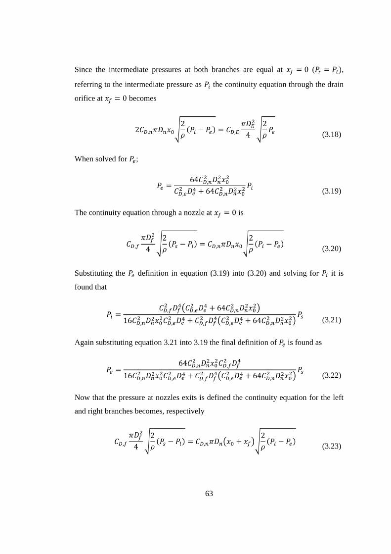
63

Since the intermediate pressures at both branches are equal at 𝑥𝑓 = 0 (𝑃𝑟 = 𝑃𝑙),

referring to the intermediate pressure as 𝑃𝑖 the continuity equation through the drain

orifice at 𝑥𝑓 = 0 becomes

2𝐶𝐷,𝑛𝜋𝐷𝑛𝑥0√

2

𝜌(𝑃𝑖 − 𝑃𝑒) = 𝐶𝐷,𝐸

𝜋𝐷𝐸2

4√2

𝜌𝑃𝑒

(3.18)

When solved for 𝑃𝑒;

𝑃𝑒 =

64𝐶𝐷,𝑛2 𝐷𝑛

2𝑥02

𝐶𝐷,𝑒2 𝐷𝑒4 + 64𝐶𝐷,𝑛

2 𝐷𝑛2𝑥02 𝑃𝑖 (3.19)

The continuity equation through a nozzle at 𝑥𝑓 = 0 is

𝐶𝐷,𝑓

𝜋𝐷𝑓2

4√2

𝜌(𝑃𝑠 − 𝑃𝑖) = 𝐶𝐷,𝑛𝜋𝐷𝑛𝑥0√

2

𝜌(𝑃𝑖 − 𝑃𝑒) (3.20)

Substituting the 𝑃𝑒 definition in equation (3.19) into (3.20) and solving for 𝑃𝑖 it is

found that

𝑃𝑖 =

𝐶𝐷,𝑓2 𝐷𝑓

4(𝐶𝐷,𝑒2 𝐷𝑒

4 + 64𝐶𝐷,𝑛2 𝐷𝑛

2𝑥02)

16𝐶𝐷,𝑛2 𝐷𝑛2𝑥0

2𝐶𝐷,𝑒2 𝐷𝑒4 + 𝐶𝐷,𝑓

2 𝐷𝑓4(𝐶𝐷,𝑒

2 𝐷𝑒4 + 64𝐶𝐷,𝑛2 𝐷𝑛2𝑥0

2)𝑃𝑠

(3.21)

Again substituting equation 3.21 into 3.19 the final definition of 𝑃𝑒 is found as

𝑃𝑒 =

64𝐶𝐷,𝑛2 𝐷𝑛

2𝑥02𝐶𝐷,𝑓

2 𝐷𝑓4

16𝐶𝐷,𝑛2 𝐷𝑛2𝑥0

2𝐶𝐷,𝑒2 𝐷𝑒4 + 𝐶𝐷,𝑓

2 𝐷𝑓4(𝐶𝐷,𝑒

2 𝐷𝑒4 + 64𝐶𝐷,𝑛2 𝐷𝑛2𝑥0

2)𝑃𝑠

(3.22)

Now that the pressure at nozzles exits is defined the continuity equation for the left

and right branches becomes, respectively

𝐶𝐷,𝑓

𝜋𝐷𝑓2

4√2

𝜌(𝑃𝑠 − 𝑃𝑙) = 𝐶𝐷,𝑛𝜋𝐷𝑛(𝑥0 + 𝑥𝑓)√

2

𝜌(𝑃𝑙 − 𝑃𝑒) (3.23)

64

𝐶𝐷,𝑓

𝜋𝐷𝑓2

4√2

𝜌(𝑃𝑠 − 𝑃𝑟) = 𝐶𝐷,𝑛𝜋𝐷𝑛(𝑥0 − 𝑥𝑓)√

2

𝜌(𝑃𝑟 − 𝑃𝑒) (3.24)

The rest of the procedure is the same as it is for Model 1. By substituting the 𝑃𝑒

definition given in equation (3.22) into (3.23) and (3.24) and solving for 𝑃𝑙 and 𝑃𝑟,

the intermediate pressure definitions for both branches are found and control

pressure can be defined as it is given in equation (3.10). Then equations (3.11) and

(3.16) are evaluated to find the curtain length that yields the maximum pressure

sensitivity as

�̃�0 =√2𝐶𝐷,𝑓

2 𝐷𝑓4√𝐶𝐷,𝑒

4 𝐷𝑒8 + 4𝐶𝐷,𝑓

2 𝐷𝑓4𝐶𝐷,𝑒

2 𝐷𝑒4 + 𝐶𝐷,𝑓

4 𝐷𝑓8 − 2𝐶𝐷,𝑓

4 𝐷𝑓8 − 𝐶𝐷,𝑓

2 𝐷𝑓4𝐶𝐷,𝑒

2 𝐷𝑒4

48𝐶𝐷,𝑛2 𝐷𝑛

2(𝐶𝐷,𝑒2 𝐷𝑒

4 + 4𝐶𝐷,𝑓2 𝐷𝑓

4) (3.25)

Evaluation of Model 3 is very similar to Model 2’s except for the definition of flow

rate through nozzle, which is this time given as

𝑄 = 𝐶𝐷,𝑣𝐶𝐷,𝑛𝜋𝐷𝑛

2(𝑥0 ± 𝑥𝑓)

√16𝐶𝐷,𝑣2 (𝑥0 ± 𝑥𝑓)2 + 𝐶𝐷,𝑛

2 𝐷𝑛2√2

𝜌(𝑃𝑖 − 𝑃𝑒)

(3.26)

To define the exit pressure 𝑃𝑒 first, the continuity equation through the drain orifice

is written in the same way as equation (3.18);

2

𝐶𝐷,𝑣𝐶𝐷,𝑛𝜋𝐷𝑛2𝑥0

√16𝐶𝐷,𝑣2 𝑥0 + 𝐶𝐷,𝑛

2 𝐷𝑛2√2

𝜌(𝑃𝑖 − 𝑃𝑒) = 𝐶𝐷,𝑒

𝜋𝐷𝑒2

4√2

𝜌𝑃𝑒

(3.27)

Solving for 𝑃𝑒 it is found that

𝑃𝑒 =

64𝐶𝐷,𝑛2 𝐶𝐷,𝑣

2 𝐷𝑛2𝑥0

2

𝜆𝑃𝑖 (3.28)

where

65

𝜆 = 64𝐶𝐷,𝑛

2 𝐶𝐷,𝑣2 𝐷𝑛

2𝑥02 + 𝐶𝐷,𝑒

2 𝐷𝑒4(16𝐶𝐷,𝑣

2 𝑥02 + 𝐶𝐷,𝑛

2 𝐷𝑛2)

(3.29)

The continuity equation through a nozzle at 𝑥𝑓 = 0 is

𝐶𝐷,𝑓

𝜋𝐷𝑓2

4√2

𝜌(𝑃𝑠 − 𝑃𝑖) =

𝐶𝐷,𝑣𝐶𝐷,𝑛𝜋𝐷𝑛2𝑥0

√16𝐶𝐷,𝑣2 𝑥0 + 𝐶𝐷,𝑛

2 𝐷𝑛2√2

𝜌(𝑃𝑖 − 𝑃𝑒)

(3.30)

Substituting the 𝑃𝑒 definition in equation (3.28) into (3.30) and solving for 𝑃𝑖 it is

found that

𝑃𝑖 =

𝐶𝐷,𝑓2 𝐷𝑓

4𝜆

𝐶𝐷,𝑓2 𝐷𝑓

4𝜆 + 16𝐶𝐷,𝑛2 𝐶𝐷,𝑣

2 𝐶𝐷,𝑒2 𝐷𝑛4𝐷𝑒4𝑥0

2 𝑃𝑠 (3.31)

Again substituting equation (3.28) into (3.31) the final definition of 𝑃𝑒 is found as

𝑃𝑒 =

64𝐶𝐷,𝑛2 𝐶𝐷,𝑣

2 𝐶𝐷,𝑓2 𝐷𝑛

2𝐷𝑓4𝑥0

2

𝐶𝐷,𝑓2 𝐷𝑓

4𝜆 + 16𝐶𝐷,𝑛2 𝐶𝐷,𝑣

2 𝐶𝐷,𝑒2 𝐷𝑛4𝐷𝑒4𝑥0

2 𝑃𝑠 (3.32)

Now that the pressure at nozzles exits is defined the continuity equation for the left

and right branches becomes, respectively

𝐶𝐷,𝑓𝜋𝐷𝑓

2

4√2

𝜌(𝑃𝑠 − 𝑃𝑙)

=𝐶𝐷,𝑣𝐶𝐷,𝑛𝜋𝐷𝑛

2(𝑥0 + 𝑥𝑓)

√16𝐶𝐷,𝑣2 (𝑥0 + 𝑥𝑓)2 + 𝐶𝐷,𝑛

2 𝐷𝑛2√2

𝜌(𝑃𝑙 − 𝑃𝑒)

(3.33)

𝐶𝐷,𝑓𝜋𝐷𝑓

2

4√2

𝜌(𝑃𝑠 − 𝑃𝑟)

=𝐶𝐷,𝑣𝐶𝐷,𝑛𝜋𝐷𝑛

2(𝑥0 − 𝑥𝑓)

√16𝐶𝐷,𝑣2 (𝑥0 − 𝑥𝑓)2 + 𝐶𝐷,𝑛

2 𝐷𝑛2√2

𝜌(𝑃𝑟 − 𝑃𝑒)

(3.34)

66

The rest of the procedure is the same as the previous models. By substituting the 𝑃𝑒

definition given in equation (3.32) into (3.33) and (3.24) and solving for 𝑃𝑙 and 𝑃𝑟,

the intermediate pressure definitions for both branches are found and control

pressure can be defined as it is given in equation (3.10). Then equations (3.11) and

(3.16) are evaluated to find �̃�0, but the definition will not be given here explicitly

since this time it is a little overcrowded. One could use an equation manipulator such

as MATLAB’s Symbolic Math Toolbox® to obtain the definition. MATLAB code

for this purpose is given in Appendix A for reference.

Numerical values of discharge coefficients used in the models are given Table 3.11.

Table 3.11 – Discharge coefficients used with the models

Variable Value Notes

CD,f 0.733 Table 3.10

CD,n 0.816 For Model 3 (Table 3.10)

0.600 For Model 1 and 2 [7]

CD,v 0.900 Table 3.10

CD,e 0.700 [7]

And for the diameters, it is assumed that fixed orifice diameter is equal to nozzle

diameter while the exit orifice diameter is twice of it. With these values �̃�0

estimations of three models are given in Table 3.12.

Table 3.12 – �̃�𝟎 estimations of the models

Model �̃�𝟎

1 0.1763𝐷𝑛

2 0.1657𝐷𝑛

3 0.0844𝐷𝑛

CFD analyses are conducted using the same configuration with the models, at �̃�0

values given in Table 3.12, with a similar set up given in Table 3.9. 𝑥0 values of

0.0625𝐷𝑛 and 0.125𝐷𝑛 are also included in the analyses to expand the data for

easier interpretation. Pressure sensitivity values are calculated for three 𝑥𝑓 values,

67

namely 0.005𝐷𝑛, 0.015𝐷𝑛 and 0.025𝐷𝑛, to also see the change in the pressure

sensitivity with respect to flapper position. Results are given in Figure 3.22.

Figure 3.22 – First stage pressure sensitivity analysis results

Figure 3.22 shows that Model 3 yields much better results than 1 and 2. But spline

interpolation curves indicates that the maximum pressure sensitivity actually occurs

around 𝑥0 = 0.1𝐷𝑛 for 𝑥𝑓 = 0. To make the model more accurate compared to CFD

results, 𝐶𝐷,𝑣 value found previously as 0.9 is updated since it is actually a function of

𝑥𝑓. From the CFD analysis it found that at 𝑥0 = 0.1𝐷𝑛, 𝐶𝐷,𝑣 ≈ 0.75. So, when the

𝐶𝐷,𝑣 used with Model is updated to 0.75, �̃�0 is calculated as 0.1012𝐷𝑛.

Pressure sensitivity at this �̃�0 value is also calculated with CFD and it is found to be

0.0352𝑃𝑠, 0.0340𝑃𝑠 and 0.0322𝑃𝑠 at the 𝑥𝑓 values of 0.005𝐷𝑛, 0.015𝐷𝑛 and

0.025𝐷𝑛, respectively. These values are consistent with the prediction of spline

interpolation.

0.06 0.08 0.1 0.12 0.14 0.16 0.180.01

0.015

0.02

0.025

0.03

0.035

X: 0.1Y: 0.0333

x0 (D

n)

Kp

s (P

s)

[m

-1]

X: 0.15Y: 0.02273

xf = 0.005D

n

xf = 0.015D

n

xf = 0.025D

n

Model 1

Model 2

Model 3

Kps

= Pc/x

f

68

The value of 0.75 for 𝐶𝐷,𝑣 also makes more sense than 0.9 since it is more consistent

with the common knowledge that the discharge coefficients of sharp edged orifices

range from 0.6 to 0.8. So the value of 0.75 will be used for 𝐶𝐷,𝑣 in the final model.

Final set of discharge coefficients are given in Table 3.11.

Table 3.15.

Table 3.13 – Final set of discharge coefficients

Variable Value

CD,f 0.733

CD,n 0.816

CD,v 0.750

CD,e 0.700

𝐶𝐷,𝑣 is updated to increase the �̃�0 estimation accuracy of Model 3 so it is now even

superior than models 1 and 2. But one could question this approach since 𝐶𝐷,𝑛 of

models 1 and 2 can be updated as well so they could match the performance of

Model 1. The �̃�0 definition found with Model 1 in equation (3.17) can be equated to

0.1𝐷𝑛 and solved for 𝐶𝐷,𝑛 to find the 𝐶𝐷,𝑛 value that makes the Model 1 to lead to

the same result as the CFD analysis yields, which actually is found as 1.06. This

value is beyond the physical limits for a discharge coefficient which cannot be

greater than 1. The same thing can be done with equation (3.25) of Model 2 to find

that 𝐶𝐷,𝑛 should be 0.994 this time which is just as unreasonable. Even if the

physical meaning is disregarded, such a drastic change in 𝐶𝐷,𝑛 would lead to other

calculation errors such as flow rate estimation.

Another point arises from Figure 3.22 that should be taken into consideration is that

pressure sensitivity changes as the flapper moves when 𝑥0 is around 0.1𝐷𝑛, but it

seems insensitive to flapper position when 𝑥0 is around 0.15𝐷𝑛. This indicates that

when the pressure sensitivity at 𝑥𝑓 = 0 is maximized the linearity of the output with

respect to flapper motion is adversely affected. By increasing 𝑥0 towards 0.15𝐷𝑛 the

69

pressure sensitivity could be compromised in favour of linearity. So, there is a trade-

off between the pressure sensitivity and linearity and for some cases the first stage

design may need to be made carefully.

One could also question the necessity of the inclusion of the exit pressure into the

model, which complicates things incredibly. To clarify this issue, definition of �̃�0 is

found for Model 3 with 𝑃𝑒 = 0 in equations (3.33) and (3.24) using the MATLAB

code given in Appendix A. Result is found as;

�̃�0 =𝐶𝐷,𝑓𝐶𝐷,𝑛𝐷𝑓

2𝐷𝑛

4𝐶𝐷,𝑣√3(𝐶𝐷,𝑓2 𝐷𝑓

4 + 𝐶𝐷,𝑛2 𝐷𝑛4)

(3.35)

Substituting discharge coefficients with their respective values given in Table 3.13,

equation (3.35) is reevaluated for different 𝐷𝑓 values and results are given in Table

3.14.

Table 3.14 – �̃�𝟎 values calculated with equation (3.35)

𝑫𝒇 (× 𝑫𝒏) �̃�𝟎 (× 𝑫𝒏)

0,5 0,0344

0,75 0,0708

1 0,105

On the other hand �̃�0 values for Model 3 with respect to 𝐷𝑒 is plotted in comparison

to the results in Table 3.14 in Figure 3.23. The figure shows that although the error

rate increases as the fixed orifice diameter increases, equation (3.35) estimates �̃�0

pretty close to Model 3 if 𝐷𝑒 ≥ 2𝐷𝑛. Since a practical servovalve is likely to have

𝐷𝑒 ≥ 2𝐷𝑛, first stage model can be simplified by omitting exit pressure with a little

loss in accuracy.

70

Figure 3.23 – Comparison of �̃�𝟎 values found with or without 𝑷𝒆

Spool Valve Model

Overlap and underlap conditions in a spool valve imply two different geometrical

conditions; therefore, at least two different functions should be used to define the

flow rates in these conditions. In order these two functions to form a continuous flow

curve throughout the entire spool position range to overcome the non-smooth

transition problem mentioned in Section 2.4, they must abide by the following

constraints:

𝑄𝑈𝐿|𝐿=0 = 𝑄𝑂𝐿|𝐿=0

(3.36)

1 1.5 2 2.5 3 3.5 4 4.5 50

0.01

0.02

0.03

0.04

0.05

0.06

0.07

0.08

0.09

0.1

De (D

n)

x0 (

Dn)

Model 3 w/ Pe

Model 3 w/o Pe

Df = 0.75D

n

Df = 0.5D

n

Df = D

n

71

𝜕𝑄𝑈𝐿𝜕𝐿

|𝐿=0

=𝜕𝑄𝑂𝐿𝜕𝐿

|𝐿=0

(3.37)

In equations (3.36) and (3.37), 𝑄𝑈𝐿 and 𝑄𝑂𝐿 are the flow rate functions for underlap

and overlap conditions, respectively. Equation (3.36) implies that at the transition

point (𝐿 = 0) two functions must yield the same result. Similarly, equation (3.37)

implies that the slopes of both functions must be the same at this transition point. As

the starting point, standard form of the well-known orifice equation that defines the

flow rate through a spool valve in underlap condition is revisited;

𝑄𝑈𝐿 = 𝐶𝐷,𝑠𝐴√2

𝜌∆𝑃

(3.38)

To increase the accuracy, the orifice area “𝐴” in equation (3.38) is defined as the

truncated conical area between the spool and sleeve as shown in Figure 3.24.

Figure 3.24 – The truncated conical area between the spool and the sleeve

The area of this truncated cone is given by

𝐴 = 𝜋(𝑅 + 𝑟)√𝐵2 + 𝐿2

(3.39)

Since 𝑅 ≈ 𝑟, this area can be approximately written as follows:

𝐴 = 2𝜋𝑅√𝐵2 + 𝐿2

(3.40)

SLEEVE

SLEEVE

L

SPOOL

LR

72

Substituting this area expression into equation (3.38), 𝑄𝑈𝐿 becomes

𝑄𝑈𝐿 = 2𝐶𝐷,𝑠𝜋𝑅√𝐵2 + 𝐿2√2

𝜌∆𝑃

(3.41)

The function defining the flow rate in overlap condition is developed based on

equation (1). The problem with equation (1) is the term with L being alone in the

denominator. In order to prevent singularity as L approaches to zero, another term

(𝑀) is added to the denominator

𝑄𝑂𝐿 =

𝜋𝑅𝐵3

6𝜇𝐿 +𝑀∆𝑃

(3.42)

Note that in equation (2.28) the effect of eccentricity between the spool and sleeve is

taken into account. According to equation (2.28) when the spool is 100% eccentric,

the flow rate is 2.5 times more than it would be if it was concentric with the sleeve.

But the effect of eccentricity becomes important only when 𝐿 ≫ 𝐵. As 𝐿 approaches

zero, the effect of eccentricity diminishes, becoming totally ineffective at zero-

lapped condition. That is because the pressure drop is caused by the sudden decrease

in the area through which the fluid passes, rather than the shear forces between the

fluid and walls as it was if the fluid flowed through an annulus. When the spool

comes to zero-lapped position, the eccentricity does not affect the amount of

reduction in area. So the term representing eccentricity in equation (2.28) is

neglected in equation (3.42), since the port lappings of a spool valve are assumed to

deviate around zero with a small amount.

The definition of “𝑀” in equation (3.42) is found by evaluating equation (3.43).

2𝐶𝐷,𝑠𝜋𝑅𝐵√2

𝜌∆𝑃 =

𝜋𝑅𝐵3

𝑀∆𝑃

(3.43)

Solving for 𝑀 yields

73

𝑀 =

𝐵2√2𝜌∆𝑃

4𝐶𝐷,𝑠

(3.44)

Now that equation (3.36) is satisfied, equation (3.37) can be worked on to complete

the model. The slope of equation (3.42) at 𝐿 = 0 is found as

𝜕𝑄𝑂𝐿𝜕𝐿

|𝐿=0

=6𝜇𝜋𝑅𝐵3∆𝑃

(6𝜇𝐿 +𝐵2√2𝜌∆𝑃4𝐶𝐷,𝑠

)

2|

|

𝐿=0

= −48𝐶𝐷,𝑠

2 𝜇𝜋𝑅

𝜌𝐵

(3.45)

while the slope of equation (3.41) at 𝐿 = 0 becomes

𝜕𝑄𝑈𝐿𝜕𝐿

|𝐿=0

=2𝐶𝐷,𝑠𝜋𝑅√

2𝜌∆𝑃

√𝐵2 + 𝐿2||

𝐿=0

= 0

(3.46)

It is obvious that slopes of equations (3.41) and (3.42) when 𝐿 = 0 cannot be equal

in their current forms. But if the discharge coefficient 𝐶𝐷,𝑠 is treated as a function of

𝐿 rather than treating it as a constant this problem can be resolved. The importance

of treating the discharge coefficient as a variable was already underlined in the

literature [42]. Using variable𝐶𝐷,𝑠, the slope of equation (3.41) at 𝐿 = 0 becomes

𝜕𝑄𝑈𝐿𝜕𝐿

|𝐿=0

=

(

𝜕𝐶𝐷,𝑠

𝜕𝐿2𝜋𝑅√𝐵2 + 𝐿2√

2

𝜌∆𝑃 +

2𝐶𝐷,𝑠𝜋𝑅√2𝜌 ∆𝑃

√𝐵2 + 𝐿2

)

𝐿=0

=𝜕𝐶𝐷,𝑠

𝜕𝐿|𝐿=0

2𝜋𝑅𝐵√2

𝜌∆𝑃

(3.47)

By using the slope matching condition dictated by equation (3.37) one gets

𝜕𝐶𝐷,𝑠

𝜕𝐿|𝐿=0

=24𝐶𝐷,0

2 𝜇

𝐵2√2𝜌∆𝑃

(3.48)

74

Equation (3.48) is the rate of change of the discharge coefficient at 𝐿 = 0 for a spool

valve control port. A discharge coefficient definition satisfying equation (3.48)

provides a continuous flow curve at all spool positions. But since equation (3.48)

cannot be solved analytically, the function defining the discharge coefficient is found

by fitting a function on the data from CFD analyses.

It is reported in the literature that the discharge coefficient is a function of Reynolds

number and the orifice geometry [7]. The Reynolds number is defined as

𝑅𝑒 =

𝜌𝑉𝐿

𝜇

(3.49)

where 𝐿 is the characteristic length of the subject geometry. The characteristic length

of the annular orifice investigated here is the radial clearance 𝐵 shown in Figure 2.7.

Furthermore, the velocity definition √2∆𝑃/𝜌 of standard orifice equation can be

used to estimate the velocity 𝑉 before the flow takes place. After these modifications

the Reynolds number estimation becomes

𝑅𝑒∗ =

𝐵√2𝜌∆𝑃

𝜇

(3.50)

Computational fluid dynamics analyses for 200 different design points are conducted

in order to characterize 𝐶𝐷,𝑠. Design points are obtained by varying 𝐵, 𝜌, ∆𝑃, and 𝜇

of equation (3.50), to calculate flow rates for each case. The results are substituted

into equation (3.41) at 𝐿 = 0 and equation (3.41) is solved for 𝐶𝐷,𝑠. This process is

repeated using different turbulence models and wall functions in the CFD solver to

determine which model demonstrates best performance by comparing 𝐶𝐷,𝑠 versus

𝑅𝑒∗ graphs.

All analyses are carried out in 2D axisymmetric domains shown in Figure 3.25 using

Fluent’s parametric analysis capability. Figure 3.26 shows the details around the

radial clearance of a sample grid that has 6217 cells with minimum orthogonal

quality of 82.8% and maximum aspect ratio of 1.66. Grids with similar quality are

75

used in all CFD analyses conducted in the analyses. Some details about mesh

generation and solution are given in Table 3.11.

Table 3.15 – Calculation details for spool valve discharge coefficient analyses

Minimum num. of cells across any gap 14

Growth rate 1.04

Maximum face size 200 μm

Convergence criteria Residuals to drop below 10-5

Pressure-Velocity coupling scheme Coupled

Discretization scheme Second order upwind for all equations

Maximum iteration 1000

Mesh adaption Every 50th iteration

Max. level of refinement for adaption 2

Adaption method Cells with at least 10% of max. velocity gradient

Figure 3.25 – Details of analysis domain

BPre

ssu

re I

nle

t

1 mmAxis of symmetry

15 mm

4 mm

Pressure Inlet

3 mm

4 m

m

Pre

ssu

re O

utl

et

76

Figure 3.26 – Details around the radial clearance in a sample grid

Each turbulence model-wall function combination yields a unique discharge

coefficient curve as given Figure 3.27. As shown in Figure 3.27, the laminar solution

is also obtained for low Reynolds numbers for comparison. It is known in the

literature that the use of scalable wall functions at low Reynolds numbers is likely to

yield inaccurate results [54]. It is apparent that solutions with scalable wall function

resulted in lower flow rate estimations comparing to laminar solution. So, it is

decided that the use of scalable wall function is inappropriate for the purposes of our

study.

On the other hand, the 𝐶𝐷,0 curve obtained using RNG k–ε + Enhanced Wall

Treatment combination is physically unrealistic because of the two local maxima it

possesses. Therefore, from the two k–ω solutions which showed very similar

performance to each other, the discharge coefficient curve of shear stress transport

(SST) k–ω solution is used as a reference to develop a mathematical model.

77

Figure 3.27 – Comparison of discharge coefficient versus Reynolds number estimation curves obtained using

different turbulence model and wall function combinations

Similar works in the literature studying the discharge coefficient on spool valves are

examined to check the degree of agreement. Posa et al. conducted numerical

analyses on 2D axisymmetric spool valve geometry, very similar to the analyses in

this work [41]. They provided a very detailed report on their work in terms of the

geometric dimensions, fluid properties, and boundary conditions that were used.

Using the same parameters with theirs, a set of CFD analyses are conducted using

SST k–ω turbulence model as opposed to their direct numerical solution approach.

The comparison of the results is given in Figure 3.28.

100

101

102

103

104

0

0.1

0.2

0.3

0.4

0.5

0.6

0.7

0.8

0.9

Reynolds number estimation (Re*)

Dis

charg

e c

oeff

icie

nt

@ L

=0 (

CD

,0)

Standard k-, Scalable Wall Func.

Realizable k-, Scalable Wall Func.

RNG k-, Scalable Wall Func.

RNG k-, Enhanced Wall Treatment

Standard k-, Low Re

+ Shear Stress Correction

SST k-, Low Re Correction

Laminar

78

Figure 3.28 – Comparison of discharge coefficient data in the paper of Posa et al. to the ones obtained by SST k–

ω turbulence model. Different discharge coefficients for same port openings are obtained by using different flow

rates.

Figure 3.28 shows the discharge coefficients found using SST k–ω are consistently

higher than the ones found in [41]. In another work by Pan et al. [40], even lower

discharge coefficients are reported. So it can be said that there is no common

agreement on the discharge characteristics of spool valves in the literature yet. One

should consider this fact before using the models provided in such works.

A mathematical function is fitted to the 𝐶𝐷,0 curve obtained from SST k–ω solution

and given in Figure 3.27. This function is given in equation (3.51), and its

performance is illustrated in Figure 3.29 comparing to CFD data.

𝐶𝐷,0 =

0.77(𝑅�̃�4 + 𝑅�̃�) exp(−0.09𝑅�̃�−0.3)

𝑅�̃�4 − 3.6𝑅�̃� + 7.2

(3.51)

where

𝑅�̃� = log(𝑅𝑒∗ + 1) (3.52)

0 0.5 1 1.5 20.5

0.55

0.6

0.65

0.7

0.75

0.8

0.85

Port opening [mm]

Dis

charg

e c

oeff

icie

nt

CFD data from Posa's work

CFD data from present work

79

Figure 3.29 – Comparison of discharge coefficient data obtained by SST k–ω turbulence model and output of

the fitted function

It should be noted that CFD analysis presented here is only conducted for 𝐿 = 0.

Therefore, discharge coefficient estimations here are named as 𝐶𝐷,0. If the spool is

moved so the orifice is underlapped, then the geometry changes. Since 𝐶𝐷,𝑠 is a

function of geometry too, there should be a term in the 𝐶𝐷,𝑠 expression to reflect the

changes in the geometry.

The general shape of the orifice between the spool and sleeve for 𝐿 < 0 with the

parameters defining it is shown in Figure 3.30.

In order to study the effects of 𝜃 in Figure 3.30 on 𝐶𝐷,𝑠, a separate set of CFD

analyses are conducted again using SST k–ω turbulence model. The graph of the

resulting data is shown in Fig. 12.

100

101

102

103

104

0

0.2

0.4

0.6

0.8

1

Reynolds number estimation (Re*)

Dis

charg

e c

oeff

icie

nt

(CD

,0)

CFD data

Output of

developed function

80

Figure 3.30 – Parameters which are used to define the underlap condition

Figure 3.31 – 𝑪𝜽 curves obtained from CFD analyses

𝐶𝜃 in Figure 3.31 is the ratio of the discharge coefficient at a certain 𝐿 value to the

𝐶𝐷,𝑠 estimation if 𝐿 = 0 with the other parameters fixed;

𝐶𝜃 = 𝑓(𝜃, 𝑅�̃�) =

𝐶𝐷,𝑠𝐶𝐷,0

(3.53)

In the analyses, 𝜃 is varied with constant 𝐿𝑒 and the Reynolds number estimation

given in equation (3.50) is updated as 𝐿𝑒√2𝜌∆𝑃/𝜇 so that the Reynolds number

estimation is kept constant as 𝜃 changes. A function is developed that would reflect

SLEEVE

SPOOLL

B

θ

100

101

102

103

104

1

1.05

1.1

1.15

1.2

1.25

1.3

1.35

1.4

Reynolds number estimation (Re*)

Dis

charg

e c

oeff

icie

nt

multip

lier

(C)

= 15o

= 30o

= 45o

81

the effect of the changes in 𝜃 on 𝐶𝜃 based on the data for 𝑅𝑒∗ < 10 and given in the

following equation:

𝐶𝜃 = 1 + (𝐶𝜃|𝜃=45° − 1)

sin 𝜃 + cos 𝜃 − 1

√2 − 1

(3.54)

Comparison of the results of equation (22) to CFD data is given in Figure 3.32.

Figure 3.32 – Change in 𝑪𝜽 with respect to 𝜽 for 𝑹𝒆∗ < 𝟏𝟎

Note that to be able to use equation (22), 𝐶𝜃 at 𝜃 = 45° must be known. So, one

final function to calculate 𝐶𝜃|𝜃=45° is developed based on the data shown in Figure

3.31;

𝐶𝜃|𝜃=45° = 1.34 − 0.31 tanh

𝑅�̃�5

20

(3.55)

Thus, the 𝐶𝜃 function takes its final form as follows

𝐶𝜃 = 1 +(0.34 − 0.31 tanh

𝑅�̃�5

20 )(sin 𝜃 + cos 𝜃 − 1)

√2 − 1

(3.56)

A comparison of the results of equation (3.56) and data in Figure 3.31 is given in

Fig. 14.

0 15 30 45 60 75 901

1.05

1.1

1.15

1.2

1.25

1.3

1.35

1.4

[o]

Dis

charg

e c

oeff

icie

nt

multip

lier

(C)

CFD data

Output of developed function

82

Figure 3.33 – Comparison of developed 𝑪𝜽 function to CFD data

At this point, the model for the calculation of flow rate at the orifices of a spool

valve is completed and given as equation (3.57).

𝑄 =

{

𝜋𝑅𝑠𝐵3

6𝜇𝐿 +𝐵2√2𝜌∆𝑃4𝐶𝐷,0

Δ𝑃 𝑖𝑓 𝐿 ≥ 0

2𝐶𝐷,𝑠𝜋𝑅𝑠√𝐵2 + 𝐿2√

2

𝜌∆𝑃 𝑖𝑓 𝐿 < 0

(3.57)

where

𝐶𝐷,𝑠 = 𝐶𝐷,0𝐶𝜃

𝐶𝐷,0 = 0.77(𝑅�̃�4 + 𝑅�̃�) exp(−0.09𝑅�̃�−0.3)

𝑅�̃�4 − 3.6𝑅�̃� + 7.2

100

101

102

103

104

1

1.05

1.1

1.15

1.2

1.25

1.3

1.35

1.4

Reynolds number estimation (Re*)

Dis

charg

e c

oeff

icie

nt

multip

lier

(C)

= 15o CFD data

= 15o Output of

developed function

= 30o CFD data

= 30o Output of

developed function

= 45o CFD data

= 45o Output of

developed function

83

𝐶𝜃 = 1 +

(0.34 − 0.31 tanh𝑅�̃�5

20 )(sin 𝜃 + cos 𝜃 − 1)

√2 − 1

𝑅�̃� = log(𝑅𝑒∗ + 1)

𝑅𝑒∗ = √𝐵2 + [min(𝐿, 0)]2√2𝜌∆𝑃

𝜇

The model is evaluated on a four-way spool valve with dimensions given in Figure

3.34 to demonstrate its performance.

Figure 3.34 – The valve geometry which is used to test final model

Calculations are carried out with 100 bar inlet pressure, 1000 kg/m3 fluid density,

and 0.02 Pa·s dynamic viscosity. The position range of the spool is assumed to be

±100 μm. A CFD analysis is conducted for the same case using SST k–ω turbulence

model, and the results are compared in Figure 3.35.

84

Figure 3.35 – Flow rate estimations of developed model and CFD analysis

It is seen in Figure 3.35 that the model yields consistent results with CFD data

especially around null position. As the spool deviates from null position, the model

suggested yields a lower flow rate estimation than the CFD analysis. This is due to

the addition of an artificial term (𝑀) to the denominator of equation (2.28).

Apparently, this term makes the resistance of the annular orifice at overlap condition

be calculated higher than it is in CFD analyses. A percentage error map between

CFD data and model’s result across the entire spool position range of Figure 3.35 is

given in Figure 3.36. It is seen in Figure 3.36 that the maximum error of the model in

this case is 13.3%. Since each port of the valve is modeled as a separate orifice, and

these orifices are connected in serial to form the overall valve simulation, the model

would work with a similar performance for any imaginable port configuration.

-100 -50 0 50 1000.1

0.2

0.3

0.4

0.5

0.6

0.7

0.8

0.9

Spool position [m]

Flo

w r

ate

fro

m P

to T

[L/m

in]

Output of

the model

CFD data

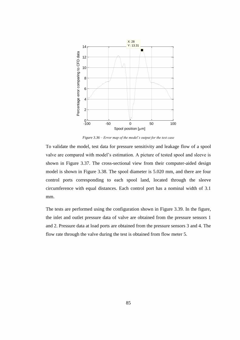
85

Figure 3.36 – Error map of the model’s output for the test case

To validate the model, test data for pressure sensitivity and leakage flow of a spool

valve are compared with model’s estimation. A picture of tested spool and sleeve is

shown in Figure 3.37. The cross-sectional view from their computer-aided design

model is shown in Figure 3.38. The spool diameter is 5.020 mm, and there are four

control ports corresponding to each spool land, located through the sleeve

circumference with equal distances. Each control port has a nominal width of 3.1

mm.

The tests are performed using the configuration shown in Figure 3.39. In the figure,

the inlet and outlet pressure data of valve are obtained from the pressure sensors 1

and 2. Pressure data at load ports are obtained from the pressure sensors 3 and 4. The

flow rate through the valve during the test is obtained from flow meter 5.

-100 -50 0 50 1000

2

4

6

8

10

12

14

X: 28

Y: 13.31

Spool position [m]

Perc

enta

ge e

rror

com

paring t

o C

FD

data

86

Figure 3.37 – A picture of the spool and the sleeve used in the tests

Figure 3.38 – Cross-sectional view of tested spool valve’s computer aided design model

87

Figure 3.39 – Hydraulic scheme of test configuration

A series of tests are performed at 165 bar of source pressure while MIL-H-5606

hydraulic oil is used. The equipment used in the test system are given in Table 3.16.

Table 3.16 – Equipment used in spool valve test system

Equipment Company Model Details

Pump Parker PV080 Variable Displacement, 80cc

Flowmeter VSE VSI 0.1 10000 pulse/L resolution, 10 L/min maximum flow rate

Pressure sensor

Trafag NAH 8254 0-60 bar measurement range, accuracy ≤ ±%0.125 FS

LVDT Applied Measurements

AML/M < ±%1.0 FS Non-Linearity < ±%0.1 FS Repeatability

Data acquisition system

National Instruments

9219 universal input module on cRIO-9064 chassis

50 Hz noise rejection mode: 130 ms conversion time

Working fluid Belgin Oil MIL-H-5606 @20 °C

88

During the tests, the spool is driven from one end to change its position, and an

linearly variable differential transformer is used to measure the position at the other

end. The valve is tested with the configuration suggested in [55], i.e., load ports are

blocked, the pressure at valve chambers and the flow rate from valve to reservoir are

measured. Under these conditions, the valve has a maximum leakage flow rate of

0.487 L/min and pressure sensitivity (i.e., slope of load pressure curve at null

position) of 29.96 bar/μm. The model’s prediction of radial clearance and port

lappings of the valve are given in Table 3.17.

Table 3.17 – Model’s prediction of valve dimensions

B (μm) LPA (μm) LAT (μm) LPB (μm) LBT (μm)

3 -4 -5 6 6

With these dimensions, model calculates a maximum leakage flow rate of 0.485

L/min and pressure sensitivity of 29.96 bar/μm. Since there are no available

measurement results for the distances between sleeve ports and spool lands, model’s

prediction for these dimensions are presented but not verified. Nevertheless, the

model estimates the leakage flow rate and pressure sensitivity with very high

accuracy capturing the shape of related curves on Figure 3.40 and Figure 3.41 very

well at the same time. Therefore, the developed model shows promise for utilization

in geometric tolerance determination of spool valves.

89

Figure 3.40 – Comparison of model’s leakage flow rate estimation to test data

Figure 3.41 – Comparison of model’s load pressure estimation to test data

-50 -40 -30 -20 -10 0 10 20 30 40 500

0.1

0.2

0.3

0.4

0.5

0.6

Spool position [m]

Leakage f

low

rate

[L/m

in]

Model's estimation

Test data

-50 -40 -30 -20 -10 0 10 20 30 40 50-200

-150

-100

-50

0

50

100

150

200

Spool position [m]

Load p

ressure

[bar]

Model's estimation

Test data

90

91

CHAPTER 4

4. COMPLETE DYNAMICAL MODEL OF A DOUBLE STAGE NOZZLE-FLAPPER

SERVOVALVE

A nonlinear model in Simulink® environment using SimScape® blocks reflecting

all the nonlinearities that are observed in a is developed in this chapter.

Ouline of the nonlinear model created in SimScape is shown in Figure 4.1.

Figure 4.1 – Outline of the SimScape Model

As seen in the figure, valve is split into three main components: Armature Assembly,

First Stage and Second Stage. Torque input to the armature assembly is calculated by

multiplying the input current by a torque constant 𝑘𝑇, while the supply pressure 𝑃𝑠 is

supplied to the system using a “Pressure Source” block which supplies constant

pressure during the simulation.

92

In what follows the three main components are explained in detail.

SimScape Model

Armature Assembly

Armature assembly component takes the torque produced by the torque motor (𝑇𝑚),

the torque produced by the fluid jets ejected from the nozzles (𝑇𝑛) and spool position

information to calculate the force applied by the feedback spring as its inputs.

Outputs of it are the flapper speed/position and the force from the feedback spring

applied to the spool in the second stage. Details of the component are shown in

Figure 4.2.

Figure 4.2 – Details of Armature Assembly Component

1

2

3

4

6

7

5

93

What is done in Armature Assembly component is basically the solution of equation

(2.1) which is given below for reference.

𝑇𝑡𝑚 + 𝑇𝑛 = 𝐽𝐹𝑆�̈� + 𝑐𝐹𝑆�̇� + 𝑘𝑓𝑏𝐿𝑓(𝑥𝑠 + 𝑥𝑓) + 𝑘𝑓𝑡𝜃 (2.1)

Referring to Figure 4.2, the torque summation “𝑇𝑡𝑚 + 𝑇𝑛” is carried out and supplied

to an “Ideal Torque Source” block at (1). At (3), the flexure tube stiffness (𝑘𝑓𝑡) and

armature damping (𝑐𝐹𝑆) are introduced to the system, and a hard stop is used to

simulate the case in which the flapper hits against the nozzles. The motion sensor at

(2) extracts the position and velocity information of the inertia defined at (5) to

supply to the first stage and for monitoring. At (4) the rotational position of flapper

is converted to translational position at the nozzle axis (refer to Figure 2.3) to be

supplied to First Stage component. At (6) rotational properties of the armature

assembly is converted translational properties via a “Rack & Pinion” block to couple

its information with spool’s so the force exerted by the feedback spring on both the

armature and spool can be calculated. At (7) this information is supplied to a

“Translational Spring” block to simulate the feedback spring. The torque sensors

seen in the figure are used for monitoring purposes.

First Stage

First Stage component takes the flapper position information from Armature

Assembly, calculates spool control pressures and the torque caused by the fluid jets

from the nozzles on the flapper for a given supply pressure. The details of the

component are shown in Figure 4.3.

Referring to Figure 4.3, the flapper position information is taken in and curtain areas

for each nozzle branch is calculated at (1). At (2), supply pressure information is

taken in and fed to the fixed orifices at each branch. At (3), pressure information

between the fixed orifices and nozzles are fed to second stage. At (4) the nozzles are

simulated as shown in Figure 3.11. At (5) the equations (2.2) to (2.6) are carried out

94

to calculated 𝑇𝑛, and the information is supplied to Armature Assembly component.

At (6) the flow rate from the nozzles to the servovalve outlet port measured and

monitored, which is the “tare flow” of the servovalve [55]. Finally, the drain orifice

of the servovalve (refer to Figure 3.21) is simulated at (7) using a Fixed Orifice

block.

Figure 4.3 – Details of First Stage Component

Second Stage

Second Stage component takes control pressures and feedback spring force as its

inputs and calculates simulates spool motion and flow through the spool ports. Its

details are shown in Figure 4.4.

1

5

23

4

76

95

Figure 4.4 – Details of Second Stage Component

In Figure 4.4, the pressures information from both branches of the first stage in

imported and used for calculation of the driving force of the spool at (1). Here the

spool is modeled using a “Double-Acting Hydraulic Cylinder” block which lets the

information of spool area, maximum stroke and dead volumes at the ends so it can

account for the compressibility of the fluid. The mass, damping and friction on the

spool are defined at (3). The damping coefficient is defined as it is given in equation

(2.25). Also, the Bernoulli force is defined at (3) as a spring having a stiffness

coefficient given in equation (4.5). A custom block is created to simulate the

Bernoulli force with the source code given in Appendix C. If equation (2.24) was

1

5

2

3

4

96

used directly to define the Bernoulli force it would cause convergence problems at

𝑥𝑠 = 0 since 𝑥𝑠 is in the denominator.

Figure 4.5 – Relation between the control pressure and no-load flow rate

The test data given in Figure 4.5 shows the relation between the control pressure and

no-load flow rate of a double stage servovalve. The hysteresis in the test data is

caused by the hysteresis of the sensors, and orientation difference of the spool when

moving in different directions. Since control pressure creates the force on the spool

which balances the Bernoulli force, and there is a linear relation between the flow

rate and the spool position, the data in Figure 4.5 can be used to interpret the relation

between the spool position and Bernoulli force. According to the data, Bernoulli

force can be modeled as a spring force;

𝐹𝐵 = 𝑘𝐵𝑥𝑠 (4.1)

-20 -15 -10 -5 0 5 10 15 20-15

-10

-5

0

5

10

15

No-Load Flow Rate [L/min]

Contr

ol P

ressure

[bar]

data1

linear

97

One may prefer to model the Bernoulli force as a linear spring force accepting a

small amount of error. If the control pressure and spool position data is available 𝑘𝐵

can be defined as a constant;

𝑘𝐵 =

𝑃𝑐,𝑚𝑎𝑥𝐴𝑠𝑥𝑠,𝑚𝑎𝑥

(4.2)

where 𝑥𝑠,𝑚𝑎𝑥 is the maximum spool position and 𝑃𝑐,𝑚𝑎𝑥 is the control pressure at

𝑥𝑠,𝑚𝑎𝑥. Alternatively, it can be estimated as it is done in equation (2.39);

𝑘𝐵 = 0.77𝐶𝐷,𝑠

2 𝑤(𝑃𝑠 − 𝑃𝐿) (4.3)

Equation (4.3) can be further simplified substituting 𝐶𝐷,𝑠 with its asymptotical value

0.77 as found in equation (3.51). Also, since servovalves’ performance tests are

conducted theoretically in no-load flow condition (see Section 4.1.3 for more detail),

load pressure 𝑃𝐿 can also be neglected to finally get;

𝑘𝐵 = 0.46𝑤𝑃𝑠 (4.4)

The 0.46 constant in the formula can be named as Bernoulli force constant (𝐾𝐵) and

can be tuned for different valves if the test data is available. Also, one should be

aware of the fact that the pressure drop across the second stage can actually never be

equal to supply pressure 𝑃𝑆 on the entire working range since there will be a certain

amount of resistance to flow at the entry, the exit and the line connecting the load

ports of the servovalve in reality. This effect is the reason that the slope of the curve

in Figure 4.5 decreases as the flow rate increases. So, in reality, equation (4.4)

should be expressed in terms of pressure drop across the second stage instead of

supply pressure;

𝑘𝐵 = 𝐾𝐵𝑤∆𝑃𝑆𝑆 (4.5)

Turning back to Figure 4.4, at (2) spool motion information is shared with First

Stage component to be used for the calculation of feedback spring force. At (4) spool

position and velocity is exported for monitoring purposes.

98

At (5), the spool ports are simulated to calculate the flow rate during the simulation.

Each “Spool Port” component here simulates one of the four ports of the 4-way

valve used in the second stage of double-stage servovalve. Name convention for the

ports is as shown in Figure 1.1. The Spool Port component is compiled as a custom

SimScape block using the model derived in Section 3.2.1 with the source code given

in Appendix D. The user interface of the block is shown in Figure 4.6, where the

user must enter the spool radius, radial clearance, the ratio of sleeve perimeter which

is used as port (see Figure 3.37) and the lapping of the port at null position. The

block has three connection ports as seen in Figure 4.4, where U and D are the ports

for upstream and downstream flow lines and S is the position signal. Positive

position signal closes the port while negative one opens it.

Figure 4.6 – Custom spool port block user interface

Although both stages of a servovalve is supplied from the same pressure source (i.e.,

pump), a separate “Pressure Source” block is used in the simulation for Second

Stage since the numerical stability could not be sustained when the same pressure

source with the First Stage is used.

The ports are connected in the “No-Load Flow Test” configuration in Figure 4.4 as

per SAE ARP 490 [55]. Hydraulic scheme of this configuration is also showed in

Figure 4.7.

99

Figure 4.7 – No-Load Flow test configuration hydraulic scheme

In this configuration the output characteristics of the servovalve such as maximum

no-load flow rate, linearity or null region can be quantified. The other test

configuration is “Leakage Flow Test Configuration”, the hydraulic scheme of which

is shown in Figure 3.39. A servovalves pressure sensitivity (or pressure gain) and

maximum internal leakage is measured using that configuration. The model shown

in Figure 4.4 can easily be changed to leakage flow configuration by simply

changing the flow rate sensor with a pressure sensor. Full list of performance metrics

of a servovalve and their definitions are given in detail in SAE ARP 490 [55].

Also note that in Figure 4.4 there is a fixed orifice at the upstream of the spool ports

used to account for the flow resistances of the inlet and the outlet of the servovalve

manifold. It is possible to use separate fixed orifices for inlet and oulet but a single

100

orifice is preferred here combining the effects of both to keep the number of

components low. A servovalve must be so designed that pressure drop is kept as low

as possible between the inlet port and spool ports, or the spool ports and the return

port. Otherwise the pressure drop across the second stage cannot be kept constant

throughout the working range and this affects the output linearity adversely.

Simulation of Moog 31 Series Servovalve

To test the created model, parameter set of a commercial valve, namely Moog Series

31 Nozzle-Flapper Servovalve is used. Parameters and output performance of this

valve are made available by the manufacturer in [5] and given in Appendix E.

Despite the parameters are originally given in imperial units, they are converted to SI

units and given in Table C.1. Note that armature related stiffness, damping and

inertia parameters are given 𝑁𝑚 𝑚⁄ , 𝑁𝑚 (𝑚/𝑠 )⁄ and 𝑁𝑚 (𝑚/𝑠2 )⁄ to be used in

direct calculation of the flapper states 𝑥𝑓, 𝑥�̇� and 𝑥�̈�. But the equations of motion of

the model which is constructed for this study are based on armature rotation, not the

flapper translation. Since the relation between the armature rotation and flapper

position is given by 𝑥𝑓 = 𝐿𝑓𝜃, 𝐿𝑓 must be determined in order to make the

parameters compatible with the present model. 𝐿𝑓 is not provided in the datasheet,

but the external dimensions (Figure C.1) and a cross sectional view of the servovalve

are given (Figure 4.8). Using the given information, 𝐿𝑓 and 𝐿𝑠 of the valve is

approximated by determining the distances in pixels on Figure 4.8 and mapping

them on a known dimension. This dimension is chosen to be the middle axis of

torque motor connector and the lower end of the valve manifold, which is given as

34.8 mm in Figure C.1.

101

Figure 4.8 – Cross sectional view of Moog Series 31 Servovalve [4]

The related distances are found using the program WebPlotDigitizer [56]. The image

that is imported to the program is given in Figure 4.9.

The distances measured are namely the connector middle line (which approximately

coincides with armature middle line) to flexure tube base, to nozzle axis (see Figure

2.3), to spool axis and to manifold lower end. Since connector middle line to

manifold lower end distance is known as 34.8 mm the other are interpolated

according to that distance. The results are given in clearer view in Figure 4.10. Since

Figure 4.10 is a schematic view the dimensions are not in correct scale on with the

figure.

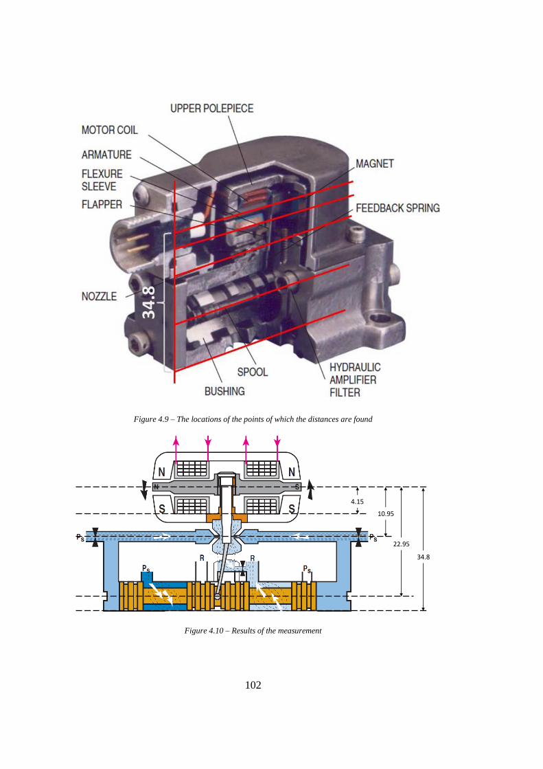
102

Figure 4.9 – The locations of the points of which the distances are found

Figure 4.10 – Results of the measurement

4.15

10.95

22.95

34.8

103

Since the pivot point of the flapper should lie somewhere in the middle of the 4.15

mm dimension (see Appendix B), half of this dimension is subtracted from 10.95

and 22.95 to estimate 𝐿𝑓 and 𝐿𝑠, which are found as 8.87 and 20.87 mm,

respectively.

Now that 𝐿𝑓 and 𝐿𝑠 is known, armature related parameters can be transformed as

given in Table 4.1.

Table 4.1 – Converted parameters

Parameter Originally Relation Value

𝑘𝐴 𝑘𝑓 𝑘𝐴 = 𝑘𝑓𝐿𝑓 4.53 N.m/rad

𝑘𝑓𝑏 𝑘𝑤 𝑘𝑓𝑏 = 𝑘𝑤/𝐿𝑠 3560 N/m

𝑏𝐴 𝑏𝑓 𝑏𝐴 = 𝑏𝑓𝐿𝑓 6.3·10-4 N.m/(rad/s)

𝐽𝐴 𝐽𝑓 𝐽𝐴 = 𝐽𝑓𝐿𝑓 1.74·10-7 N.m/(rad/s2)

The sleeve in Figure 3.37 is actually the sleeve of a Moog Series 31 Servovalve. Its

rectangular ports’ total width on one section, i.e., the port gradient 𝑤 is measured as

12 mm. Spool weight is measured as 3 gr. The fixed orifice measured in Section 3.1

is also from a Moog Series 31 Servovalve, so assuming same diameter for nozzle

exit and fixed orifice 200 μm is used for both dimensions. Also assuming 40 μm for

𝑥0, 2 μm for 𝐵 [57] and completely neglecting the spool damping as suggested in

Section 2.3. The only parameter that is left undetermined is the area of the orifice

which is used to simulate the resistance to low in the second stage apart from the

metering ports. Since it is known that the valve provides 15.1 L/min control flow at

𝑥𝑠 = 381 μm, the pressure drop can be found using equation (2.34);

15.1𝐿𝑚𝑖𝑛

1000𝐿𝑚3 ∙ 60

𝑠𝑚𝑖𝑛

= .77(12 ∙ 10−3𝑚)(381 ∙ 10−6𝑚)√∆𝑃

860𝑘𝑔𝑚3

→ ∆𝑃 = 44 𝑏𝑎𝑟

104

It is also given that this flow rate is obtained at 70 bar supply pressure, so the flow

resistance of the valve manifold must cause a 26 bar pressure drop at 15.1 L/min

flow rate. Therefore using standard orifice formula;

15.1𝐿𝑚𝑖𝑛

1000𝐿𝑚3 ∙ 60

𝑠𝑚𝑖𝑛

= 𝐶𝐷𝐴√2

860𝑘𝑔𝑚3

(26 ∙ 105 𝑃𝑎) → 𝐶𝐷𝐴 = 3.24 𝑚𝑚2

In the Fixed Orifice block used to account for manifold resistance in the simulation

model, discharge coefficient 𝐶𝐷 can simply be defined as unity and area 𝐴 can be

defined as 3.24 mm2. With the area defining the entry resistance is determined, the

complete set of parameters used in the simulation is become as given in Appendix F.

With these parameters spool position and control flow graphs are given in Figure

4.11.

Figure 4.11 – Spool position and control flow rate graphs with initial parameter set

0 5 10 15 20 25 30 35 40 45 500

100

200

300

400 X: 50

Y: 316.4

Time [ms]

Spool positio

n [

m]

0 5 10 15 20 25 30 35 40 45 500

5

10

15

X: 50

Y: 13.47

Time [ms]

Contr

ol flow

[L/m

in]

105

The simulation has underestimated the control flow by ~10% than the datasheet

value 15.1 L/min. But note that the parameters given in datasheet are given for a

much simpler linear model shown in Figure 4.12.

Figure 4.12 – The model suggested in Moog Type 30 Servovales catalogue [5]

The model shown in Figure 4.12 doesn’t take many effects into consideration such

as the torque applied by the nozzle jets on the flapper or the feedback springs effect

on spool. These effects may not be significant when singled out, but their absence

together can explain the 10% underestimation of the flow rate. It should also be

considered that the parameters given in the datasheet are probably tuned for the

model in Figure 4.12. Also, the parameters 𝐿𝑓 and 𝐿𝑠 are extracted from the picture

of the valve (Figure 4.8), while 𝐷𝑛 and 𝑥0 are guessed based on assumptions. So,

these parameters can be tuned with the constants of the present model to fit the

available data. For this purpose, the parameters given in Table 4.2 are updated to the

given values.

Table 4.2 – Updated parameters

Parameter New value

𝐷𝑛 235 μm

𝑥0 35 μm

𝐿𝑓 9,85 mm

𝐿𝑠 19,87 mm

𝑘𝑓𝑏 3300 N/m

𝐾𝐵 0.45

106

With the updated parameters results becomes as shown in Figure 4.13.

Figure 4.13 - Spool position and control flow rate graphs with updated parameter set

As shown in the figure, static spool position and control flow performance meets the

datasheet values now. Bode plot of the valve is predicted as shown in Figure 4.14

with 210 bar supply pressure and ±25% of the full input (2.5 mA). It is seen that the

-3 dB magnitude frequency is 77.4 Hz and -90° phase lag is at 337 Hz, which is

given as >200 Hz in the data sheet.

0 5 10 15 20 25 30 35 40 45 500

100

200

300

400

X: 50

Y: 385.3

Time [ms]

Spool positio

n [

m]

0 5 10 15 20 25 30 35 40 45 500

5

10

15

20

X: 50

Y: 15.32

Time [ms]

Contr

ol flow

[L/m

in]

107

Figure 4.14 – Bode plot prediction with the updated parameters

The control flow curve with the new parameters is given in Figure 4.15. Maximum

nonlinearity is calculated as 7% explained in SAE ARP 490. This value also is given

in the datasheet as ≤7%. By switching to leakage flow test configuration as

explained in Section 4.1.3, valves load pressure and spool leakage curves are also

obtained and given in the figures Figure 4.16 and Figure 4.17. As seen in Figure

4.16, the load pressure increases to 40% of supply pressure in 0.2% of the rated

current and the maximum spool leakage is 0.35 L/min which should be <1.2% and

<1 L/min, respectively according to the datasheet. Note that all metering ports on the

second stage are critically lapped in the simulation which is very hard to manage in

reality. The tare flow of the valve is also obtained as 0.37 L/min which should be

lower than 0.45 L/min again according to the datasheet. By changing all the

parameters one can see the variations in the servovalve performance and this is the

power of the developed simulation model. For example if all the metering ports were

5 μm overlapped, these graphs would become as shown in figures Figure 4.18 to

Bode Diagram

100

101

102

103

-135

-90

-45

0

System: estsys8

I/O: Step to Control Flow Rate

Frequency (Hz): 337

Phase (deg): -90

Phase (

deg)

-15

-10

-5

0From: Step To: Control Flow Rate

Magnitude (

dB

)

System: estsys8

I/O: Step to Control Flow Rate

Frequency (Hz): 77.4

Magnitude (dB): -3

108

Figure 4.20. Note that overlapping the valve decreases its pressure sensitivity and

creates a dead zone around null position in the no-load flow curve.

Figure 4.15 – Predicted no-load flow curve of Moog Series 31 Servovalve

Figure 4.16 – Predicted load pressure curve of Moog Series 31 Servovalve

-10 -8 -6 -4 -2 0 2 4 6 8 10-20

-15

-10

-5

0

5

10

15

20

Input current [mA]

Contr

ol flow

rate

[L/m

in]

Flow gain line

Max. nonlinearity

-1 -0.8 -0.6 -0.4 -0.2 0 0.2 0.4 0.6 0.8 1-250

-200

-150

-100

-50

0

50

100

150

200

250

X: 0.03325

Y: 84

X: 0.01158

Y: -8.882e-16

Input current [mA]

Load p

ressure

[bar]

109

Figure 4.17 - Predicted spool leakage curve of Moog Series 31 Servovalve

Figure 4.18 – No-load flow curve with 5 μm overlapped metering ports

-1 -0.8 -0.6 -0.4 -0.2 0 0.2 0.4 0.6 0.8 10.05

0.1

0.15

0.2

0.25

0.3

0.35

0.4X: 0

Y: 0.3527

Input current [mA]

Spool le

akage [

L/m

in]

-10 -8 -6 -4 -2 0 2 4 6 8 10-20

-15

-10

-5

0

5

10

15

20X: 10

Y: 15.21

Input current [mA]

No-load f

low

rate

[L/m

in]

110

Figure 4.19 – Load pressure curve with 5 μm overlapped metering ports

Figure 4.20 – Spool leakage curve with 5 μm overlapped metering ports

If all the ports were underlapped by 5 μm, a higher flow gain region would be

created around the null position of the no-load flow curve as shown in Figure 4.21.

-1 -0.8 -0.6 -0.4 -0.2 0 0.2 0.4 0.6 0.8 1-250

-200

-150

-100

-50

0

50

100

150

200

250

X: 0.01158

Y: 4.08e-06

X: 0.08932

Y: 84

-1 -0.8 -0.6 -0.4 -0.2 0 0.2 0.4 0.6 0.8 10.04

0.06

0.08

0.1

0.12

0.14

0.16

X: 0.002198

Y: 0.1425

Input current [mA]

Spool le

akage [

L/m

in]

111

Its load pressure and spool leakage curves would become as shown in Figure 4.22

and Figure 4.23. As seen the spool leakage greatly increases by underlapping the

ports exceeding maximum leakage of 1 L/min given in the datasheet.

As shown in the examples, little deviations in the geometric dimensions of a

servovalve ccan cause drastic changes in the performance. With the developed

model, effects of all the parameters on a servovalves performance can be examined.

This could be helpful in many ways, such as determining geometric tolerances or

diagnosing a servovalve if the performance data is available.

Figure 4.21 – No-load flow curve with 5 μm underlapped metering ports

-10 -8 -6 -4 -2 0 2 4 6 8 10-20

-15

-10

-5

0

5

10

15

20X: 10

Y: 15.47

Input current [mA]

No-load f

low

rate

[L/m

in]

112

Figure 4.22 – Load pressure curve with 5 μm underlapped metering ports

Figure 4.23 – Spool leakage curve with 5 μm underlapped metering ports

-1 -0.8 -0.6 -0.4 -0.2 0 0.2 0.4 0.6 0.8 1-250

-200

-150

-100

-50

0

50

100

150

200

250

X: 0.02298

Y: 1.268e-06

X: 0.05325

Y: 84

-1 -0.8 -0.6 -0.4 -0.2 0 0.2 0.4 0.6 0.8 10

0.2

0.4

0.6

0.8

1

1.2

1.4 X: -0.02328

Y: 1.248

Input current [mA]

Spool le

akage [

L/m

in]

113

CHAPTER 5

5. SUMMARY AND CONCLUSIONS

Summary

In the present study, a simulation model for double stage nozzle-flapper type

electrohydraulic servovalves is developed. Motivation behind this attempt is to

create a complete servovalve model that simulates the effects of all the geometric

dimensions on its performance so it can be used as a geometric tolerance analysis

tool. The model simulates the effects of several critical parameters of a servovalve

on its performance, such as port lappings, first stage geometric dimensions, manifold

resistance, fluid properties, etc.

The development process begins with summarizing the existing relations defining

servovalve hydraulics and underlining their deficiencies. Then more accurate

analytical models are developed, starting with a nozzle-flapper valve model, which

is used as the first stage of a double stage servovalve combined with a pair of fixed

orifices. For model development, most accurate turbulence models and wall

functions are determined by comparing fixed orifice experimental pressure drop vs.

flow rate data with the ones found using numerical analyses. After that, a more

accurate analytical model for nozzle-flapper valve is suggested. The model treats the

nozzle as a combination of a fixed and a variable orifice connected in serial, as

opposed to the common approach of modeling it as just a variable orifice. The

suggested first stage model needs three discharge coefficients to be determined, one

for the fixed orifice of the first stage and two for the nozzle. By the help of CFD

again, discharge coefficients related to fixed orifice and nozzles are determined

numerically.

114

Another model is developed for the second stage of the servovalve, i.e., the spool

valve. The problem of invalidity of the equation that defines the relation between the

pressure drop and flow rate for an annular gap (i.e., the overlapped case) around zero

lap length is solved by modifying the existing expression. This modification is

carried out by introducing a new constant to the denominator to prevent it to go to

zero as lap length approaches to zero. The definition of this constant is found by

imposing the constraint that implies the equations defining the flow rates for

underlapped and overlapped cases should yield the same result at zero lap length. To

ensure that the transition between these equations is smooth, another constraint is

imposed equating the slopes of the equations at zero lap length. This second

constraint led to the result that the discharge coefficient for a spool valve port must

be modeled as a variable to make the smooth transition possible. Then, the discharge

coefficient is determined by the help of CFD as a function of Reynolds’ number and

geometry, and the model is completed.

By combining the developed models in the SimScape® environment, a complete

servovalve model is created as the result.

Conclusions

Performance of the model is tested using the parameters provided by the Moog, Inc.

for their Series 31 Servovalve [4]. Many parameters, which are missing in the

datasheet, are predicted to use them with the model. Despite this prediction probably

has errors, the model is able to yield accurate results. So, it is concluded that the

model is promising, and by further tuning with more reliable datasets it could be

used as a geometric tolerance analysis or a diagnosis tool with a high accuracy.

Lastly, the effects of changing the port lappings on the servovalve static performance

metrics no-load flow, pressure sensitivity and spool leakage are examined using the

model and the results are discussed. Such analyses can be made for all the other

115

parameters by the help of the developed model to aid the designers with finding the

best dimensions to meet the performance requirements, determination of the

tolerances for these dimensions and understand the servovalve behavior under

different conditions.

Recommendations for Future Work

Since a full set of parameters is not available for the servovalve modeled and

investigated in this study, only a partial validation of the model is carried out in this

thesis. So, there is still room for a much reliable validation and update to increase the

accuracy if a complete and correct set of parameters and performance data could be

obtained.

Moreover, the present model is developed for the hydraulics of a servovalve, but the

torque motor component is not modeled in detail. Efforts should be made towards

building a detailed torque motor model and integrate it into the present model.

116

117

REFERENCES

[1] The McGraw-Hill Companies, Inc., Dictionary of Engineering, 2. Ed.,

McGraw-Hill, 2003.

[2] Moog GmbH, «D634-P Series Direct Drive Proportional Valve».

[3] J. Blackburn, G. Reethof ve J. Shearer, Fluid Power Control, Massachusetts:

The MIT Press, 1960.

[4] Moog Inc., «Type 30 Nozzle-Flapper Flow Control Servovalves».

[5] A. Plummer, «Electrohydraulic servovalves – past, present, and future,» 10th

International Fluid Power Conference, Dresden, 2016.

[6] Parker Hannifin Corporation, «Parker Abex Jet-Pipe® Servovalves - Model

425».

[7] MTS Systems Corporation, «Series 256 Servovalves».

[8] H. E. Merritt, Hydraulic Control Systems, NY: John Wiley & Sons Inc., 1967.

[9] J. Watton, Fundamentals of Fluid Power Control, Cambridge: Cambridge

University Press, 2009.

[10] D. Gall ve F. Steghart (Tinsley Industrial Instruments Ltd), «Improvements in

or relating to Servo Systems». Patent: GB620688, March 1949.

[11] H. B. Kolm-Jr., «Flow Control Servo Valve with Dynamic Load Pressure

Feedback». ABD Patent: 3,095,906, 2 June 1963.

[12] W. B. Lloyd, «Pressure Feedback Servo Valve». ABD Patent: 2,889,815, 9 June

1959.

[13] J. W. Blanton, «Servo Valve with Flow Rate Feedback». ABD Patent:

3,054,388, 18 September 1962.

[14] A. C. Lancaster Jr. ve D. I. H. Tonawanda (Moog Servocontrols), «Mechanical

Feedback Flow Control Servo Valve». East Aurora, N.Y. Patent: 3,023,782, 6

118

March 1962.

[15] S. Karunanidhi ve M. Singaperumal, «Mathematical modelling and

experimental characterization of a high dynamic servo valve integrated with

piezoelectric actuator,» J. Systems and Control Engineering, vol. 224, pp. 419-

432, 2010.

[16] S. Karunanidhi ve M. Singaperumal, «Design, analysis and simulation of

magnetostrictive actuator and its application to high dynamic servo valve,»

Sensors and Actuators A, vol. 157, pp. 185-197, 2010.

[17] Alibaba Group, «Jack Ma on the China Opportunity at Gateway '17,» 21 June

2017. [Online]. Available: https://www.youtube.com/watch?v=B0vkX-CzKTY.

[Accessed: 11 November 2017].

[18] M. Ivantysynova, «Technologies and Innovations for Hydraulic Pumps,» 10th

International Fluid Power Conference, Dresden, 2016.

[19] W. Anderson, Controlling Electrohydraulic Systems, New York: Marcel

Dekker, Inc., 1988.

[20] M. G. Rabie, Fluid Power Engineering, McGraw Hill, 2009.

[21] S. J. Lin ve A. Akers, «The Predicted Performance of a Flapper-Nozzle Valve:

Comparison with Expretiment,» American Control Conference, Atlanta, USA,

1988.

[22] D. McCloy ve H. R. Martin, Control of Fluid Power, Analysis and Design,

Halsted Press, 1980.

[23] S. J. Lin ve A. Akers, «A Dynamic Model of the Flapper-Nozzle Component of

an Electrohydraulic Servovalve,» Journal of Dynamic Systems Measurement

and Control, no. 111, pp. 105-109, 1989.

[24] S. J. Lin ve A. Akers, «A Nonlinear Model of a Flapper-Nozzle Valve,»

American Control Conference, Pittsburgh, USA, 1989.

[25] N. Z. Aung, Q. Yang, M. Chen ve S. Li, «CFD analysis of flow forces and

energy loss characteristics in a flapper–nozzle pilot valve with different null

clearances,» Energy Conversion and Management, no. 83, p. 284–295, 2014.

119

[26] Y. Zhu ve S. Fei, «Design criterion involving comprehensive performance

characteristics of nozzle–flapper valves,» J Systems and Control Engineering,

vol. 5, no. 230, pp. 452-466, 2016.

[27] L. Li, H. Yan, H. Zhang ve J. Li, «Numerical simulation and experimental

research of the flow force and forced vibration in the nozzle-flapper valve,»

Mechanical Systems and Signal Processing, no. 99, p. 550–566, 2017.

[28] A. Kılıç, S. Kapucu, S. Bayseç ve J. R. Jones, «İki kademeli elektro hidrolik

valfin kanatçık valf modeli ve kanatçık nozul boşluğu basıncının incelenmesi,»

VIII. Ulusal Hidrolik Pnömatik Kongresi, İzmir, 2017.

[29] J. Watton, «The Effect of Drain Orifice Damping on the Performance

Characteristics of a Servovalve Flapper/Nozzle Stage,» Journal of Dynamic

Systems, Measurement, and Control, vol. 109, no. 1, pp. 19-23, 1987.

[30] A. Ellman, K. Koskinen ve M. Vilenius, «Through-Flow in Short Annulus of

Fine Clearance,» International Mechanical Engineering Congress and

Exposition, San Francisco, CA, 1995.

[31] A. Ellman, «Leakage Behaviour of Four-Way Servovalve,» Fluid Power

Systems and Technology, vol. 5, pp. 163-167, 1998.

[32] A. Ellman ve T. Virvalo, «Formation of Pressure Gain in Hydraulic

Servovalves and its Significance in System Behavior,» International

Mechanical Engineering Congress and Exposition, Atlanta, GA, 1996.

[33] B. Eryılmaz ve B. H. Wilson, «Combining Leakage and Orifice Flows in a

Hydraulic Servovalve Model,» Journal of Dynamic Systems, Measurement and

Control, vol. 122, pp. 576-579, 1999.

[34] M. Feki ve E. Richard, «Including Leakage Flow in the Servovalve Static

Model,» International Journal of Modelling and Simulation, vol. 25, no. 1, pp.

51-56, 2005.

[35] S. Mookherjee, S. Acharyya, K. Majumdar ve D. Sanyal, «Static-performance

based computer-aided design of a DDV and its sensistivity analysis,»

International Journal of Fluid Power, vol. 2, no. 2, pp. 47-63, 2001.

120

[36] D. Gordić, M. Babić ve N. Jovičić, «Modelling of Spool Position Feedback

Servovalves,,» International Journal of Fluid Power, vol. 5, no. 1, pp. 37-51,

2004.

[37] D. Gordić, M. Babić, D. Milanovic ve S. Savic, «Spool Valve Leakage

Behaviour,» Arch Civil Mech Eng, pp. 859-866, 2011.

[38] T. Nakada ve Y. Ikebe, «Measurement of unsteady axial flow force on a spool

valve,» IFAC Pneumatic & Hydraulic Components, pp. 193-198, 1980.

[39] Y. Ikebe ve H. Ohuchi, «Generalized formulation of momentum theory,»

Fluidic Quarterly, no. 10, pp. 27-46, 1978.

[40] A. C. Afatsun ve T. Balkan, «(In Turkish) Orifis Akışı Çözümlemelerinde

Türbülans Modellerinin Başarımlarının Karşılaştırılması,» HPKON 2017, İzmir,

2017.

[41] X. Pan, G. Wang ve Z. Lu, «Flow field simulation and a flow model of servo-

valve spool valve orifice,» Energy Conversion and Management, no. 52, p.

3249–56, 2011.

[42] A. Posa, P. Oresta ve A. Lippolis, «Analysis of a directional hydraulic valve by

a Direct Numerical Simulation using an immersed-boundary method,» Energy

Conversion and Management, no. 65, p. 497–506, 2013.

[43] J. R. Valdes, J. M. Rodriguez, J. Saumell ve T. Pütz, «A methodology for the

parametric modelling of the flow coefficients and flow rate in hydraulic

valves,» Energy Conversation and Management, no. 33, pp. 598-611, 2014.

[44] J. R. Valdes, M. J. Miana, J. L. Nunez ve T. Pütz, «Reduced order model for

estimation of fluid flow and flow forces in hydraulic proportional valves,»

Energy Conversation and Management, no. 49, pp. 1517-29, 2008.

[45] M. K. Mondal, N. K. Manna ve R. Saha, «Study of leakage flow through a

spool valve under blocked-actuator port condition - Simulation and

experiment,» J Mechanical Engineering Science, vol. 8, no. 228, p. 1405–17,

2014.

[46] K. O. Eyyüpoglu, «Development of a novel surface damping treatment (M.Sc.

121

Thesis),» Middle East Technical University, Ankara, 2016.

[47] ANSYS, Inc., ANSYS Fluent Theory Guide, Canonsburg, PA: ANSYS, Inc.,

2017.

[48] P. Promvonge ve K. Silapabanleng, «Simulation of Turbulent Flow through a

Circular Orifice,» 13th National Mechanical Engineering Conference, South

Pattaya, Cholburi, 1999.

[49] MATLAB R2013b Simscape Hydraulic Fluid Database.

[50] K. W. Linfield, «A study of the discharge coefficient of jets from angled slots

and conical orifices (Ph.D. Thesis),» University of Toronto, 2000.

[51] J. H. L. V ve J. H. L. (IV), «Velocity Coefficients For Free Jets From Sharp-

Edged Orifices,» Journal of Fluids Engineering, vol. 106, pp. 13-17, 1984.

[52] C. L. Hollingshead, «Discharge Coefficient Performance of Venturi, Standard

Concentric Orifice Plate, V-Cone, and Wedge Flow (M.Sc. Teshis),» Utah State

University, 2011.

[53] H. D. Burghardt, Machine Tool Operation - Part II: Drilling Machine, Shaper

and Planer, Milling and Grinding Machines, Spur Gears and Bevel Gears, NY:

McGraw-Hill Book Company, 1922.

[54] F. Moukalled, L. Mangani ve M. The Finite Volume Method Darwish, The

Finite Volume Method in Computational Fluid Dynamics, Cham, Switzerland:

Springer International Publishing, 2015.

[55] SAE, «ARP 490: Electrohydraulic Servovalves,» SAE International,

Warrendale, PA, 1993.

[56] «WebPlotDigitizer,» [Online]. Available: https://automeris.io/WebPlotDigitizer.

[Accessed: 30 03 2019].

[57] R. Park, «Contamination Control - A Hydraulic OEM Perspective,» Moog

Australia Pty Ltd, Melbourne, 1997.

[58] F. Beer, E. Johnston, J. DeWolf ve D. Mazurek, Mechanics of Materials (5th

Ed.), Singapore: McGraw-Hill, 2009.

122

123

APPENDICES

A. MATLAB Codes

Linearization of the definitions of torque applied on the flapper by the fluid jets

exiting the nozzles and the control force on the spool (i.e., 𝑇𝑛 and 𝐹𝑐);

syms Ps Pl Pr Cdf Cdn rho xf Dn Df x0 Lf Ds xsd theta

An = pi*Dn^2/4;

As = pi*Ds^2/4;

xf = Lf*theta

Qfl = Cdf*pi*Df^2/4*sqrt(2/rho*(Ps-Pl));

Qnl = Cdn*pi*Dn*(x0+xf)*sqrt(2/rho*Pl);

Pl = solve(Qfl == Qnl - As*xsd, Pl);

Pl = Pl(2);

Qnl = Cdn*pi*Dn*(x0+xf)*sqrt(2/rho*Pl);

ul = Qnl/An;

Fnl = An*(Pl + 1/2*rho*ul^2);

Qfr = Cdf*pi*Df^2/4*sqrt(2/rho*(Ps-Pr));

Qnr = Cdn*pi*Dn*(x0-xf)*sqrt(2/rho*Pr);

Pr = solve(Qfr == Qnr + As*xsd, Pr);

Pr = Pr(2);

Qnr = Cdn*pi*Dn*(x0-xf)*sqrt(2/rho*Pr);

ur = Qnr/An;

Fnr = An*(Pr + 1/2*rho*ur^2);

Tn = Lf*(Fnl-Fnr);

D_Tn = subs(diff(Tn,theta),[theta xsd],[0 0])* theta +

subs(diff(Tn,xsd),[ theta xsd],[0 0])*xsd;

Fc = As*(Pr-Pl);

D_Fc = subs(diff(Fc,theta),[theta xsd],[0 0])* theta +

subs(diff(Fc,xsd),[ theta xsd],[0 0])*xsd;

124

Symbolic manipulation to find �̃�0 definition for Model 3;

syms Cdf Cdv Cdn Cde Df De Dn x0 xf rho Ps Pr Pl Pe

Cd1=Cdv*Cdn*Cde; %For simplification

Cd2=Cdv*Cdn*Cdf; %For simplification

L = Cde^2*De^4*(16*Cdv^2*x0^2+Cdn^2*Dn^2)+64*Cdv^2*Cdn^2*Dn^4*x0^2; %Lambda

Qfr = Cdf*pi*Df^2/4*sqrt(2/rho*(Ps-Pr)); %Fixed orifice flow rate (right)

Qnr = Cdv*Cdn*pi*Dn^2*(x0-xf)/sqrt(16*Cdv^2*(x0-xf)^2+Cdn^2*Dn^2)...

*sqrt(2/rho*(Pr-Pe)); %Nozzle flow rate (right)

Qfl = Cdf*pi*Df^2/4*sqrt(2/rho*(Ps-Pl)); %Fixed orifice flow rate (left)

Qnl = Cdv*Cdn*pi*Dn^2*(x0+xf)/sqrt(16*Cdv^2*(x0+xf)^2+Cdn^2*Dn^2)...

*sqrt(2/rho*(Pl-Pe)); %Nozzle flow rate (left)

Pr = solve(Qfr == Qnr,Pr); %Pressure at right branch

Pl = solve(Qfl == Qnl,Pl); %Pressure at left branch

Pc = Pr-Pl; %Control pressure

Pe_d = 64*Cd2^2*Df^4*Dn^4*x0^2*Ps/(16*Cd1^2*Dn^4*De^4*x0^2+Cdf^2*Df^4*L;

%Exit pressure definition

DPc = subs(diff(Pc,xf),[xf Pe],[0 Pe_d)]); %Control pressure sensitivity at

xf=0

x0_max = solve(diff(DPc,x0),x0); %Curtain length for max. control pressure

sensistivity (2 roots obtained)

x0_max = x0_max(2); %Second root is the positive one

Symbolic manipulation to find �̃�0 definition for Model 3 with 𝑃𝑒 = 0;

syms Cdf Cdv Cdn Cde Df De Dn x0 xf rho Ps Pr Pl

Cd1=Cdv*Cdn*Cde; %For simplification

Cd2=Cdv*Cdn*Cdf; %For simplification

L = Cde^2*De^4*(16*Cdv^2*x0^2+Cdn^2*Dn^2)+64*Cdv^2*Cdn^2*Dn^4*x0^2; %Lambda

Qfr = Cdf*pi*Df^2/4*sqrt(2/rho*(Ps-Pr)); %Fixed orifice flow rate (right)

Qnr = Cdv*Cdn*pi*Dn^2*(x0-xf)/sqrt(16*Cdv^2*(x0-xf)^2+Cdn^2*Dn^2)...

*sqrt(2/rho*Pr); %Nozzle flow rate (right)

Qfl = Cdf*pi*Df^2/4*sqrt(2/rho*(Ps-Pl)); %Fixed orifice flow rate (left)

Qnl = Cdv*Cdn*pi*Dn^2*(x0+xf)/sqrt(16*Cdv^2*(x0+xf)^2+Cdn^2*Dn^2)...

*sqrt(2/rho*Pl); %Nozzle flow rate (left)

Pr = solve(Qfr == Qnr,Pr); %Pressure at right branch

Pl = solve(Qfl == Qnl,Pl); %Pressure at left branch

Pc = Pr-Pl; %Control pressure

DPc = subs(diff(Pc,xf),xf,0); %Control pressure sensitivity at xf=0

x0_max = solve(diff(DPc,x0),x0); %Curtain length for max. control pressure

sensistivity (2 roots obtained)

x0_max = x0_max(1) %First root is the positive one

125

B. Bending of flexure tube and determination of Lf and Ls

Flexure tube and flapper are two beams fixed together from one end (upper end).

The other end of the flexure tube is fixed to the valve manifold, while the other end

of the flapper is free to move.

Figure A.1 – Flexure tube and flapper

The upper end of the flexure tube is subjected to a torque from the torque motor. For

a beam which is fixed on the one end and subjected to a torque from the other,

deflection of the moving end (maximum deflection) is calculated by [58];

𝑦 = −

𝑇𝐿2

2𝐸𝐼 (A.1)

and the slope of the moving end is calculated by [58];

𝑑𝑦

𝑑𝑥= −

𝑇𝐿

𝐸𝐼 (A.2)

where 𝑇 is the torque applied, 𝐿 is the length of beam which is the length of the

thinnest section of the flexure tube, 𝐸 is the elastic modulus of the material and 𝐼 is

the bending moment of inertia of the geometry. When the torque is applied flexure

Flexure tube

FlapperValve manifold

y

x

126

tube bends and flapper rotates with it since it is free on the lower end. Center of this

rotation can be found by calculating the point a line cuts the x axis, which passes

through the point (𝑥, 𝑦) = (𝐿,−𝑇𝐿2

2𝐸𝐼) and has the slope given in equation (A.2).

A line is defined by;

𝑦 = 𝑎𝑥 + 𝑏 (A.3)

Since 𝑎 is the slope it is known that 𝑎 = −𝑇𝐿

𝐸𝐼. 𝑏 can be found by imposing the end

point constraint;

−𝑇𝐿2

2𝐸𝐼= −

𝑇𝐿

𝐸𝐼𝐿 + 𝑏 → 𝑏 =

𝑇𝐿2

2𝐸𝐼 (A.4)

So, the point this line cuts the x axis can be found by;

0 = −

𝑇𝐿

𝐸𝐼𝑥 +

𝑇𝐿2

2𝐸𝐼→ 𝑥 =

𝐿

2 (A.5)

So, the pivot point of the flapper will always be the middle point of the thinnest

section of flexure tube. 𝐿𝑓 is equal to the distance from this point to the nozzle axis,

and 𝐿𝑠 is equal to the distance from this point to the point where the feedback spring

touches the spool.

127

C. Bernoulli Force SimScape Block Source Code

component berno < foundation.mechanical.translational.branch % Bernoulli force

inputs P = { 0, 'Pa' }; % P:left end

parameters grad = { 10, 'mm' }; % Port gradient K_B = { .46, '1' }; % Bernoulli force constant end

variables x = { 0, 'm'}; end

function setup if grad <= 0 pm_error('simscape:GreaterThanZero','Spring rate' ) end end

equations v == x.der; f == K_B*grad*P*x; end

end

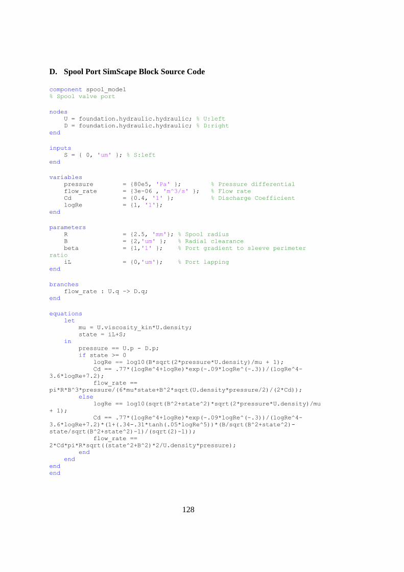
128

D. Spool Port SimScape Block Source Code

component spool_model % Spool valve port

nodes U = foundation.hydraulic.hydraulic; % U:left D = foundation.hydraulic.hydraulic; % D:right end

inputs S = { 0, 'um' }; % S:left end

variables pressure = {80e5, 'Pa' }; % Pressure differential flow_rate = {3e-06 , 'm^3/s' }; % Flow rate Cd = {0.4, '1' }; % Discharge Coefficient logRe = {1, '1'}; end

parameters R = {2.5, 'mm'}; % Spool radius B = {2,'um' }; % Radial clearance beta = {1,'1' }; % Port gradient to sleeve perimeter

ratio iL = {0,'um'}; % Port lapping end

branches flow_rate : U.q -> D.q; end

equations let mu = U.viscosity_kin*U.density; state = iL+S; in pressure == U.p - D.p; if state >= 0 logRe == log10(B*sqrt(2*pressure*U.density)/mu + 1); Cd == .77*(logRe^4+logRe)*exp(-.09*logRe^(-.3))/(logRe^4-

3.6*logRe+7.2); flow_rate ==

pi*R*B^3*pressure/(6*mu*state+B^2*sqrt(U.density*pressure/2)/(2*Cd)); else logRe == log10(sqrt(B^2+state^2)*sqrt(2*pressure*U.density)/mu

+ 1); Cd == .77*(logRe^4+logRe)*exp(-.09*logRe^(-.3))/(logRe^4-

3.6*logRe+7.2)*(1+(.34-.31*tanh(.05*logRe^5))*(B/sqrt(B^2+state^2)-

state/sqrt(B^2+state^2)-1)/(sqrt(2)-1)); flow_rate ==

2*Cd*pi*R*sqrt((state^2+B^2)*2/U.density*pressure); end end end end

129

E. Typical Parameters for Moog Series 31 Servovalve

Table C.1 – Typical parameters for Moog Series 31 Servovalve in SI units

Parameter Definition Value

𝑖 Torque motor current ±10 mA

𝑥𝑠 Spool displacement 381 μm max

𝑄𝑚𝑎𝑥 Servovalve control flow 15.1 L/min (@70 bar)

𝐾1 Torque motor gain 0.00282 N·m/mA

𝐾2 Hydraulic amplifier flow gain 0.0059 (L/min)/μm

𝐾3 Flow gain of spool 0.0405 (L/min)/μm

𝐴 Spool end area 16.8 mm2

𝑘𝑓 Net stiffness on armature/flapper 511 N·m/m

𝑘𝑤 Feedback spring stiffness 74.3 N·m/m

𝑏𝑓 Net damping on armature/flapper 0.071 N·m/(m/s)

𝐽𝑓 Rotational mass of armature/flapper 1.96e-5 N·m/(m/s2)

𝜔𝑛 Natural frequency of first stage 814 Hz

𝜁 Damping ratio of first stage 0.4

Figure C.1 – Dimension of Moog Series 31 Servovalve [4]

130

F. Parameter set used in Moog Series 31 Servovalve simulation

P_s = 70e5; %[Pa] Source pressure

rho = 860; %[kg/m^3] Mass density of MIL-H-5606 @20 oC

mu = .018; %[Pa*s] Dynamic viscosity of MIL-H-5606 @20 oC

beta = 1.556e9; %[Pa] Bulk modulus

k_T = 2.82; %[Nm/A] Torque motor gain

k_A = 4.53; %[Nm/rad] Armature stiffness

k_fb = 3560; %[N/m] Feedback spring stiffness

J_A = 1.74e-7; %[kg*m^2/rad] Armature intertia

b_T = 6.3e-4; %[Nm/(rad/s)] First stage damping coefficient

L_f = 8.87e-3; %[m] Pivot point to nozzle axis length

L_s = 20.87e-3; %[m] Pivot point to feedback-spring-ball-center length

C_dv = .75; %[] Discharge coef. of nozzle variable part

C_dn = .82; %[] Discharge coef. of nozzle fixed part

C_df = .73; %[] Discharge coef. of fixed orifice

C_dE = .70; %[] Discharge coef. of exit orifice

D_f = 200e-6; %[m] Fixed orifice diameter

D_n = 200e-6; %[m] Nozzle diameter

x_0 = 40e-6; %[m] Initial nozzle opening (Right)

A_entry = 3.24e-6; %[m^2] Entry orifice area

m_s = 3e-3; %[kg] Spool mass

D_s = 4.625e-3; %[m] Spool diameter

w = 12e-3; %[m] Port gradient

wr = w/pi/D_s; %[] Spool gradient (w) to perimeter (pi*D_s) ratio

B = 2e-6; %[m] Radial clearance between spool and sleeve

F_stiction = 1; %[N] Breakaway friction on the spool

F_coulomb = .8; %[N] Coulomb friction on the spool

131