University of Massachusetts Amherst University of Massachusetts Amherst ScholarWorks@UMass Amherst ScholarWorks@UMass Amherst Open Access Dissertations 2-2010 Modeling of Thermal Non-Equilibrium in Superheated Injector Modeling of Thermal Non-Equilibrium in Superheated Injector Flows Flows Shivasubramanian Gopalakrishnan University of Massachusetts Amherst Follow this and additional works at: https://scholarworks.umass.edu/open_access_dissertations Part of the Mechanical Engineering Commons Recommended Citation Recommended Citation Gopalakrishnan, Shivasubramanian, "Modeling of Thermal Non-Equilibrium in Superheated Injector Flows" (2010). Open Access Dissertations. 185. https://scholarworks.umass.edu/open_access_dissertations/185 This Open Access Dissertation is brought to you for free and open access by ScholarWorks@UMass Amherst. It has been accepted for inclusion in Open Access Dissertations by an authorized administrator of ScholarWorks@UMass Amherst. For more information, please contact [email protected].

Welcome message from author
This document is posted to help you gain knowledge. Please leave a comment to let me know what you think about it! Share it to your friends and learn new things together.
Transcript
University of Massachusetts Amherst University of Massachusetts Amherst
ScholarWorks@UMass Amherst ScholarWorks@UMass Amherst
Open Access Dissertations
2-2010
Modeling of Thermal Non-Equilibrium in Superheated Injector Modeling of Thermal Non-Equilibrium in Superheated Injector
Flows Flows
Shivasubramanian Gopalakrishnan University of Massachusetts Amherst
Follow this and additional works at: https://scholarworks.umass.edu/open_access_dissertations
Part of the Mechanical Engineering Commons
Recommended Citation Recommended Citation Gopalakrishnan, Shivasubramanian, "Modeling of Thermal Non-Equilibrium in Superheated Injector Flows" (2010). Open Access Dissertations. 185. https://scholarworks.umass.edu/open_access_dissertations/185
This Open Access Dissertation is brought to you for free and open access by ScholarWorks@UMass Amherst. It has been accepted for inclusion in Open Access Dissertations by an authorized administrator of ScholarWorks@UMass Amherst. For more information, please contact [email protected].
MODELING OF THERMAL NON-EQUILIBRIUM IN
SUPERHEATED INJECTOR FLOWS
A Dissertation Presented
by
SHIVASUBRAMANIAN GOPALAKRISHNAN
Submitted to the Graduate School of theUniversity of Massachusetts Amherst in partial fulfillment
of the requirements for the degree of
DOCTOR OF PHILOSOPHY
February 2010
Mechanical and Industrial Engineering
c© Copyright by Shivasubramanian Gopalakrishnan 2010
All Rights Reserved

MODELING OF THERMAL NON-EQUILIBRIUM IN
SUPERHEATED INJECTOR FLOWS
A Dissertation Presented
by
SHIVASUBRAMANIAN GOPALAKRISHNAN
Approved as to style and content by:
David P. Schmidt, Chair
J. Blair Perot, Member
Dimitrios Maroudas, Member
Donald Fisher, Department HeadMechanical and Industrial Engineering

To my beloved parents.
EPIGRAPH
Asato maa sadgamaya
Tamaso maa jyotirgamaya
Mrityor maa amritamgamaya
− Brihadaranyaka Upanishad 1.3.28.
From the untruth to the truth
From darkness to light
From death to immortality
ACKNOWLEDGMENTS
Though the Phd. degree is conferred on a single individual, the effort, at various
levels, to obtain this degree is almost always put in by several people. This dissertation
has a similar story and is an outcome of the support of many people without whom
this would not have been possible.
At the outset I would like to thank my advisor, Prof. David P. Schmidt. The past
6 years under his guidance has been a fantastic learning experience, one which I will
cherish for life. His openness to new ideas and willingness to try experimenting with
them is remarkable. I also thank Prof. Blair Perot for giving great support and con-
stant fresh ideas. I appreciate him being a part of my dissertation committee. I also
acknowledge the computational resources provided by him. I thank Prof. Dimitrois
Maroudas for serving on my dissertation committee and providing an extra dimension
to it.
I acknowledge the technical contributions and criticisms provided by Dr. Ron
Grover of GM and Dr. Jerry Lee of UTRC. I also acknowledge the support provided
by Dr. Hrvoje Jasak of Wikki ltd. This work was done with the financial support of
NASA under Contract No.NNC07CB05C.
I would like to thank my parents and my brother, Hari. They have been an
amazing source of constant support and encouragement. I am eternally indebted to
my parents, who sacrificed so much for the education that me and my brother received
and also for supporting every decision I took in my career.
During the past 6 years at the CFD lab, I was fortunate to interact with several
bright minds. The list of people I got know as colleagues and friends is just way too
vi

long for this section. I would like acknowledge each and every one for a wonderful
time and sharing their brilliant ideas.
I would also like to express gratitude to all my close friends, both near and far,
who have given me encouragement, been with me through rough times and shared
good times. You all know who you are and how much you mean to me. Finally, I
would like to thank my landlords, Merle and Billie Howes, who not only provided an
apartment but also a home to live in. You have been more than family to me.
vii
ABSTRACT
MODELING OF THERMAL NON-EQUILIBRIUM IN
SUPERHEATED INJECTOR FLOWS
FEBRUARY 2010
SHIVASUBRAMANIAN GOPALAKRISHNAN
B.E., UNIVERSITY OF MUMBAI, BOMBAY
Ph.D., UNIVERSITY OF MASSACHUSETTS AMHERST
Directed by: Professor David P. Schmidt
Among the many factors that effect the atomization of a fuel spray in a com-
bustion chamber, the flow characteristics of the fuel inside the injector nozzle play
significant roles. The enthalpy of the entering fuel can be elevated such that it is
higher than the local or downstream saturation enthalpy, which will result in the
flash-boiling of the liquid. The phase change process dramatically effects the flow
rate and has the potential to cause subsonic two-phase choking. The timescale over
which this occurs is comparable to the flow-through time of the nozzle and hence
any attempt to model this phenomenon needs to be done as a finite rate process. In
the past the Homogeneous Relaxation Model (HRM) has been successfully employed
to model the vaporization in one dimension. Here a full three dimensional imple-
mentation of the HRM model is presented. Validations have been presented with
experiments using water as working fluid.
For the external spray modeling, where the fuel is said to be flash boiling, the
phase change process plays a role alongside the aerodynamic breakup of the liquid
viii

and must be considered for obtaining the fuel spray characteristics. In this study the
HRM model is coupled with Linearized Sheet Instability Analysis (LISA) model, for
primary atomization, and with Taylor Analogy Breakup (TAB) model for secondary
breakup. The aerodynamic breakup model and phase change based breakup model
are designed as competing processes. The mechanism which satisfies its breakup
criterion first during time integration is used to predict resulting drop sizes.
ix
TABLE OF CONTENTS
Page
ACKNOWLEDGMENTS . . . . . . . . . . . . . . . . . . . . . . . . . . . . . . . . . . . . . . . . . . . . . vi
ABSTRACT . . . . . . . . . . . . . . . . . . . . . . . . . . . . . . . . . . . . . . . . . . . . . . . . . . . . . . . . .viii
LIST OF TABLES . . . . . . . . . . . . . . . . . . . . . . . . . . . . . . . . . . . . . . . . . . . . . . . . . . . xii
LIST OF FIGURES . . . . . . . . . . . . . . . . . . . . . . . . . . . . . . . . . . . . . . . . . . . . . . . . . .xiii
CHAPTER
1. INTRODUCTION . . . . . . . . . . . . . . . . . . . . . . . . . . . . . . . . . . . . . . . . . . . . . . . . . 1
2. INTERNAL FLOW MODELING . . . . . . . . . . . . . . . . . . . . . . . . . . . . . . . . . . 7
2.1 Modeling Approaches . . . . . . . . . . . . . . . . . . . . . . . . . . . . . . . . . . . . . . . . . . . . . 8
3. GOVERNING EQUATIONS . . . . . . . . . . . . . . . . . . . . . . . . . . . . . . . . . . . . . . 12
3.1 Homogeneous Relaxation Model . . . . . . . . . . . . . . . . . . . . . . . . . . . . . . . . . . . 13
4. NUMERICAL APPROACH . . . . . . . . . . . . . . . . . . . . . . . . . . . . . . . . . . . . . . 16
5. SOFTWARE FRAMEWORK . . . . . . . . . . . . . . . . . . . . . . . . . . . . . . . . . . . . . 21
5.1 Polyhedral Finite Volume Method . . . . . . . . . . . . . . . . . . . . . . . . . . . . . . . . . 215.2 Discretisation Operators . . . . . . . . . . . . . . . . . . . . . . . . . . . . . . . . . . . . . . . . . . 22
5.2.1 Convection Term . . . . . . . . . . . . . . . . . . . . . . . . . . . . . . . . . . . . . . . . . . 235.2.2 Gradient Term . . . . . . . . . . . . . . . . . . . . . . . . . . . . . . . . . . . . . . . . . . . . 235.2.3 Laplacian . . . . . . . . . . . . . . . . . . . . . . . . . . . . . . . . . . . . . . . . . . . . . . . . 245.2.4 Time Derivative . . . . . . . . . . . . . . . . . . . . . . . . . . . . . . . . . . . . . . . . . . . 24
5.3 Boundary Conditions . . . . . . . . . . . . . . . . . . . . . . . . . . . . . . . . . . . . . . . . . . . . 25
x

6. ATOMIZATION AND BREAKUP MODELS . . . . . . . . . . . . . . . . . . . . . 27
6.1 Linearized Instability Sheet Analysis . . . . . . . . . . . . . . . . . . . . . . . . . . . . . . . 28
6.1.1 Derivation of Sheet Thickness . . . . . . . . . . . . . . . . . . . . . . . . . . . . . . . 326.1.2 Cylindrical Jet . . . . . . . . . . . . . . . . . . . . . . . . . . . . . . . . . . . . . . . . . . . . 34
6.2 Homogenous Relaxation Model . . . . . . . . . . . . . . . . . . . . . . . . . . . . . . . . . . . . 386.3 Taylor Analogy Breakup . . . . . . . . . . . . . . . . . . . . . . . . . . . . . . . . . . . . . . . . . . 39
7. INTERNAL NOZZLE FLOW - RESULTS AND
VALIDATION . . . . . . . . . . . . . . . . . . . . . . . . . . . . . . . . . . . . . . . . . . . . . . . . . 41
7.1 Reitz Experiment . . . . . . . . . . . . . . . . . . . . . . . . . . . . . . . . . . . . . . . . . . . . . . . . 427.2 Tikhonenko Experiment . . . . . . . . . . . . . . . . . . . . . . . . . . . . . . . . . . . . . . . . . . 497.3 Fauske Experiment . . . . . . . . . . . . . . . . . . . . . . . . . . . . . . . . . . . . . . . . . . . . . . 557.4 Three Dimensional Nozzle . . . . . . . . . . . . . . . . . . . . . . . . . . . . . . . . . . . . . . . . 607.5 Conclusions . . . . . . . . . . . . . . . . . . . . . . . . . . . . . . . . . . . . . . . . . . . . . . . . . . . . . 69
8. INTERNAL FLASHING FLOW OF JP8 . . . . . . . . . . . . . . . . . . . . . . . . . 70
8.1 Multi-component Superheated JP8 Model . . . . . . . . . . . . . . . . . . . . . . . . . . . 708.2 Nozzle Results . . . . . . . . . . . . . . . . . . . . . . . . . . . . . . . . . . . . . . . . . . . . . . . . . . 74
9. SPRAY ATOMIZATION RESULTS . . . . . . . . . . . . . . . . . . . . . . . . . . . . . . 79
9.1 Drop Size Variation . . . . . . . . . . . . . . . . . . . . . . . . . . . . . . . . . . . . . . . . . . . . . . 849.2 Lagrangian Spray Calculation . . . . . . . . . . . . . . . . . . . . . . . . . . . . . . . . . . . . . 89
10.SUMMARY . . . . . . . . . . . . . . . . . . . . . . . . . . . . . . . . . . . . . . . . . . . . . . . . . . . . . . 94
10.1 Future Work . . . . . . . . . . . . . . . . . . . . . . . . . . . . . . . . . . . . . . . . . . . . . . . . . . . . 94
10.1.1 Fuel properties . . . . . . . . . . . . . . . . . . . . . . . . . . . . . . . . . . . . . . . . . . . . 9410.1.2 Validation and Adjustments of Coefficients . . . . . . . . . . . . . . . . . . . 9510.1.3 Nucleation Model . . . . . . . . . . . . . . . . . . . . . . . . . . . . . . . . . . . . . . . . . 95
BIBLIOGRAPHY . . . . . . . . . . . . . . . . . . . . . . . . . . . . . . . . . . . . . . . . . . . . . . . . . . . 96
xi

LIST OF TABLES
Table Page
7.1 Table. 1 Boundary conditions used for three dimensional injectorcase . . . . . . . . . . . . . . . . . . . . . . . . . . . . . . . . . . . . . . . . . . . . . . . . . . . . . . . . 62
xii

LIST OF FIGURES
Figure Page
5.1 Structure of OpenFOAM [38] . . . . . . . . . . . . . . . . . . . . . . . . . . . . . . . . . . . . . 21
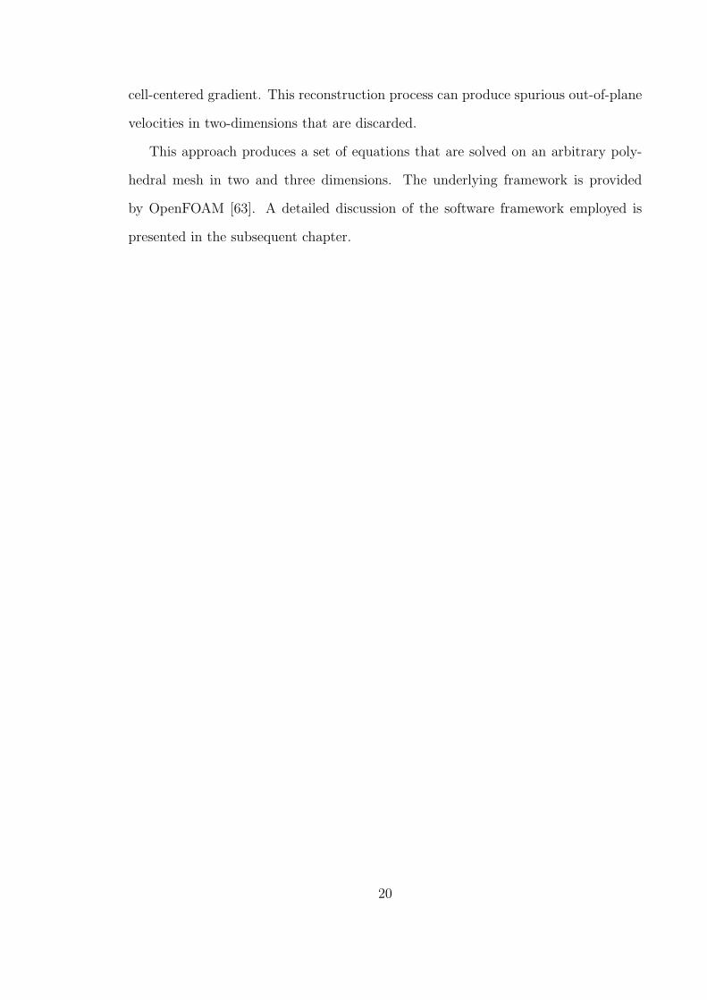
5.2 Finite Volume Discretisation [38] . . . . . . . . . . . . . . . . . . . . . . . . . . . . . . . . . . 22
6.1 Atomization of a superheated jet is brought about by two distinctbut coupled phenomena: instability at the jet/air interface andthe rapid evaporation of the superheated liquid. . . . . . . . . . . . . . . . . . . 28
6.2 Non−dimensional growth rate versus non−dimensional wave numberWe = 0.5 . . . . . . . . . . . . . . . . . . . . . . . . . . . . . . . . . . . . . . . . . . . . . . . . . . . . 30
6.3 Non−dimensional growth rate versus non−dimensional wave numberWe = 5.0 . . . . . . . . . . . . . . . . . . . . . . . . . . . . . . . . . . . . . . . . . . . . . . . . . . . . 31
6.4 Conical sheet at an angle θ . . . . . . . . . . . . . . . . . . . . . . . . . . . . . . . . . . . . . . . 33
6.5 Flowchart for coupled HRMLISA . . . . . . . . . . . . . . . . . . . . . . . . . . . . . . . . . . 36
6.6 Bubble growth and subsequent breakup into droplets . . . . . . . . . . . . . . . . . 38
6.7 Flowchart for coupled HRMTAB . . . . . . . . . . . . . . . . . . . . . . . . . . . . . . . . . . 40
7.1 A typical two-dimensional computational domain. . . . . . . . . . . . . . . . . . . . . 41
7.2 Nozzle design used by Reitz[43]. All dimensions are in centimeters. . . . . . 42
7.3 Velocity contours for inlet temperature = 404 K . . . . . . . . . . . . . . . . . . . . . 43
7.4 Density contours for inlet temperature = 404 K. . . . . . . . . . . . . . . . . . . . . . 43
7.5 Velocity contours for inlet temperature = 415 K . . . . . . . . . . . . . . . . . . . . . 44
7.6 Density contours for inlet temperature = 415 K. . . . . . . . . . . . . . . . . . . . . . 45
7.7 Velocity contours for inlet temperature = 427 K . . . . . . . . . . . . . . . . . . . . . 45
xiii

7.8 Density contours for inlet temperature = 427 K. . . . . . . . . . . . . . . . . . . . . . 46
7.9 Velocity contours for inlet temperature = 438 K . . . . . . . . . . . . . . . . . . . . . 47
7.10 Density contours for inlet temperature = 438 K. . . . . . . . . . . . . . . . . . . . . . 47
7.11 Comparison of mass flow rates between experiments andsimulations . . . . . . . . . . . . . . . . . . . . . . . . . . . . . . . . . . . . . . . . . . . . . . . . . . 49
7.12 Static pressure versus position at the wall for saturated water at 4MPa discharging through a 25 mm tube with L/D=10 . . . . . . . . . . . . . 51
7.13 Predicted vapor mass fraction and volume fraction in the 4 MPasaturated water experiment of Tikhonenko. The domain has beenreflected around the axis of symmetry so that two fields can beshown simultaneously. . . . . . . . . . . . . . . . . . . . . . . . . . . . . . . . . . . . . . . . . . 52
7.14 Predicted pressure and equilibrium mass fraction x in the 4 MPasaturated water experiment of Tikhonenko. . . . . . . . . . . . . . . . . . . . . . . 53
7.15 Predicted velocity magnitude and the common log of the phasechange timescale Θ for the 4 MPa saturated water experiment ofTikhonenko. . . . . . . . . . . . . . . . . . . . . . . . . . . . . . . . . . . . . . . . . . . . . . . . . . 54
7.16 Measured [17] mass flow rates for a nozzle with L/D=4 comparedwith the present calculations. . . . . . . . . . . . . . . . . . . . . . . . . . . . . . . . . . . 56
7.17 Simulation of Fauske’s experiment with 1.38 MPa saturated liquiddischarge. This figure shows volume fraction of vapor andapproximate streamlines. . . . . . . . . . . . . . . . . . . . . . . . . . . . . . . . . . . . . . . 57
7.18 Simulation of Fauske’s experiment with 1.38 MPa saturated liquiddischarge. This figure shows velocity magnitude and the commonlogarithm of the timescale of phase change. . . . . . . . . . . . . . . . . . . . . . . 58
7.19 Comparison of the volumetric vapor fraction with 1.38 MPa saturatedliquid discharge (upper half) and 6.89 MPa (lower half). . . . . . . . . . . . 59
7.20 Orthographic projection of the injector design obtained from BoschGmbH. . . . . . . . . . . . . . . . . . . . . . . . . . . . . . . . . . . . . . . . . . . . . . . . . . . . . . . 60
7.21 Computational domain with mesh . . . . . . . . . . . . . . . . . . . . . . . . . . . . . . . . . 61
7.22 Hexahedral mesh in nozzle . . . . . . . . . . . . . . . . . . . . . . . . . . . . . . . . . . . . . . . . 61
xiv
7.23 Orientation of the cut plane . . . . . . . . . . . . . . . . . . . . . . . . . . . . . . . . . . . . . . . 62
7.24 Velocity contours for baseline case . . . . . . . . . . . . . . . . . . . . . . . . . . . . . . . . . 63
7.25 Density contours for baseline case . . . . . . . . . . . . . . . . . . . . . . . . . . . . . . . . . . 63
7.26 Velocity contours for low flow case . . . . . . . . . . . . . . . . . . . . . . . . . . . . . . . . . 64
7.27 Density contours for low flow case . . . . . . . . . . . . . . . . . . . . . . . . . . . . . . . . . 65
7.28 Velocity contours for high flow case . . . . . . . . . . . . . . . . . . . . . . . . . . . . . . . . 65
7.29 Density contours for high flow case . . . . . . . . . . . . . . . . . . . . . . . . . . . . . . . . . 66
7.30 Velocity contours for low temperature case . . . . . . . . . . . . . . . . . . . . . . . . . . 66
7.31 Density contours for low temperature case . . . . . . . . . . . . . . . . . . . . . . . . . . 67
7.32 Velocity contours for high temperature case . . . . . . . . . . . . . . . . . . . . . . . . . 67
7.33 Density contours for high temperature case . . . . . . . . . . . . . . . . . . . . . . . . . 68
8.1 Distillation curve of surrogate fuel for JP8. Given by Lee et. al.[29] . . . . . . . . . . . . . . . . . . . . . . . . . . . . . . . . . . . . . . . . . . . . . . . . . . . . . . . . . 71
8.2 Loci of bubble and dew points for JP8. Given by Lee et. al. [29] . . . . . . . 72
8.3 Pressure and density contours for cases with back pressure of a) 9 barand b) 4bar . . . . . . . . . . . . . . . . . . . . . . . . . . . . . . . . . . . . . . . . . . . . . . . . . 76
8.4 Pressure drop along the length of the channel . . . . . . . . . . . . . . . . . . . . . . . 77
8.5 Variation of mass flow rate with inlet and back pressure . . . . . . . . . . . . . . 77
8.6 Radial variation of void fraction at injector exit . . . . . . . . . . . . . . . . . . . . . . 78
9.1 Shear instability induced breakup of a liquid jet. The liquid core canclearly be seen prior to its breakup (atomization) [30]. . . . . . . . . . . . . 80
9.2 Flash vaporization induced breakup of a superheated jet. The liquidcore disappeared and the atomization process occurs near the exitof the nozzle orifice. [30] . . . . . . . . . . . . . . . . . . . . . . . . . . . . . . . . . . . . . . 81
xv
9.3 Curves that mark the boundary in the T-P space separating theregion were atomization is effected either by the shear atomizationor flash atomization mode. Experimentally determined value of Tat 1 atmospheric pressure in the current work for this transition isshown for comparison. Additionally, a value reported at 2atmospheric pressure [56] is included as well. Plots of the loci ofthe bubble and dew points are included for comparison. . . . . . . . . . . . . 82
9.4 Variation of primary drop size, relative jet velocity = 12 m/s . . . . . . . . . . 84
9.5 Variation of secondary drop size, relative jet velocity = 12 m/s . . . . . . . . 86
9.6 Variation of primary drop size, relative jet velocity = 30 m/s . . . . . . . . . . 86
9.7 Variation of secondary drop size, relative jet velocity = 30 m/s . . . . . . . . 87
9.8 Variation of primary drop size, relative jet velocity = 50 m/s . . . . . . . . . . 88
9.9 Variation of secondary drop size, relative jet velocity = 50 m/s . . . . . . . . 89
9.10 Velocity contours, Boundary layer = 10 mm . . . . . . . . . . . . . . . . . . . . . . . . . 91
9.11 Pressure contours, Boundary layer = 10 mm . . . . . . . . . . . . . . . . . . . . . . . . 92
9.12 Particle Tracks, Boundary layer = 10 mm . . . . . . . . . . . . . . . . . . . . . . . . . . . 93
xvi
CHAPTER 1
INTRODUCTION
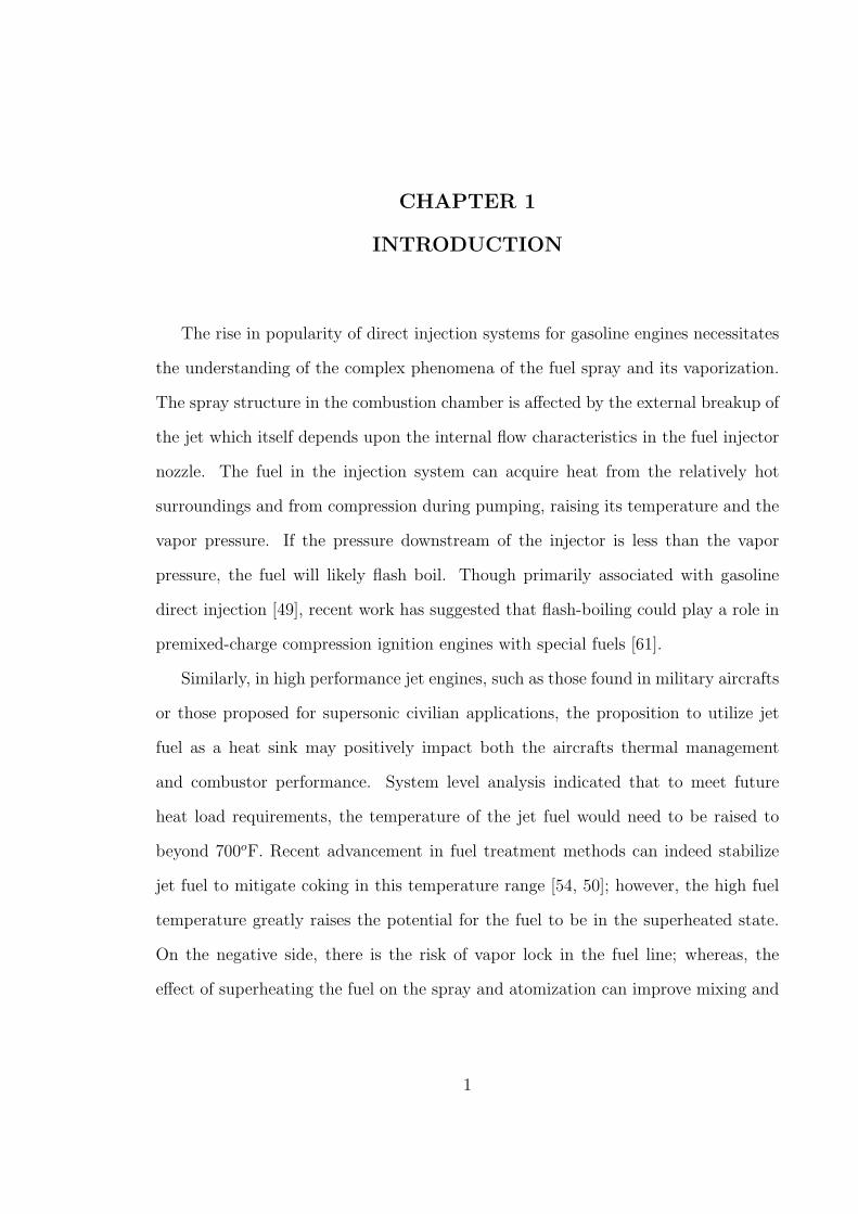
The rise in popularity of direct injection systems for gasoline engines necessitates
the understanding of the complex phenomena of the fuel spray and its vaporization.
The spray structure in the combustion chamber is affected by the external breakup of
the jet which itself depends upon the internal flow characteristics in the fuel injector
nozzle. The fuel in the injection system can acquire heat from the relatively hot
surroundings and from compression during pumping, raising its temperature and the
vapor pressure. If the pressure downstream of the injector is less than the vapor
pressure, the fuel will likely flash boil. Though primarily associated with gasoline
direct injection [49], recent work has suggested that flash-boiling could play a role in
premixed-charge compression ignition engines with special fuels [61].
Similarly, in high performance jet engines, such as those found in military aircrafts
or those proposed for supersonic civilian applications, the proposition to utilize jet
fuel as a heat sink may positively impact both the aircrafts thermal management
and combustor performance. System level analysis indicated that to meet future
heat load requirements, the temperature of the jet fuel would need to be raised to
beyond 700oF. Recent advancement in fuel treatment methods can indeed stabilize
jet fuel to mitigate coking in this temperature range [54, 50]; however, the high fuel
temperature greatly raises the potential for the fuel to be in the superheated state.
On the negative side, there is the risk of vapor lock in the fuel line; whereas, the
effect of superheating the fuel on the spray and atomization can improve mixing and
1
thus combustor performance and emissions as has been shown in experiments and
theoretical analysis performed with gasoline direction injection systems [51, 67, 64].
Flash boiling is a phenomenon similar to cavitation, which is also known to occur
in gasoline injectors [35]. Both are a transition from liquid to vapor due to a drop in
pressure. In contrast to nucleate boiling, the enthalpy for vaporization is not provided
at walls during the phase change process, but is instead provided by inter-phase heat
transfer. A gross distinction between cavitating and flash-boiling nozzle flow is simply
that the enthalpy of the cavitating flow is below the saturated liquid enthalpy at
the downstream pressure, while the enthalpy of the flash-boiling flow exceeds the
saturated liquid enthalpy at the downstream pressure. A detailed discussion of the
differences must be deferred until after some review of phase change physics.
An experimental study by Oza and Sinnamon [40] found that flashing occurred in
two modes, namely the “external flashing mode” and the “internal flashing mode.”
Park and Lee [41] performed investigations using transparent nozzles and reported
the flashing modes in the internal and the external flow. Apart from the degree of
superheat it was found that the factors affecting flash boiling included the nozzle
geometry, surface roughness, turbulence and physical properties of the fuel. The
external spray characteristics as result of flash boiling of superheated fuel have been
studied experimentally by several researchers [58, 66, 1].
Even though only a very small fraction of the liquid mass changes phase while
still in the nozzle, this small amount of mass can occupy a large volume and greatly
affect the nozzle flow. However, there are many investigations of external sprays un-
der flash-boiling conditions and relatively few studies of the internal flashing flow. As
noted by Park and Lee [41], the phase change process definitely begins within the noz-
zle. Experimental studies of flashing nozzle flow have primarily been conducted with
water, such as Reitz [43] and Fauske [17]. Fauske noted that the flow through nozzles
2
will choke under saturated conditions (with respect to the upstream conditions) and
low downstream pressure.
There have been a few attempts to model the internal flashing flow, almost all
limited to one-dimensional flow. For a recent example of one-dimensional modeling,
the reader may consult Barret et al. [2]. Such models are often not satisfactory for
the low length-to-diameter ratios used in most fuel injector nozzles, where the nozzle
flow is separated and displays two and three-dimensional features. Schmidt et al. [47]
reported the development of a two-dimensional flashing simulation for simple nozzle
shapes, which offers some insights into short flashing-nozzle flow. However, Schmidt
et al. were limited to simple, two-dimensional block-structured meshes. This initial
effort produced a code that was not terribly robust or efficient. Fortunately, the
numerical techniques available and the understanding of the special requirements of
modeling flashing flow have progressed.
Any numerical investigation in the physics of the atomization consists of two dis-
tinct sections,the external jet break up and the internal nozzle flow. The calculations
of the nozzle flow calculations serve as inputs to external jet break up models. The
external modeling of flash boiling sprays has been presented in the past by Zeng et
al. [68], Zuo et al [69], and Kawano et al. [25].
These external spray models have been developed with the best information avail-
able, but the open literature has very little to offer about the details of the internal
flashing flow. Important questions remain about the velocity of the fluid leaving the
nozzle and the fraction of vapor present at the nozzle exit. Further, we wish to know
more about how nozzle geometry and injection pressure affect the internal flow.
When a hot fluid has a vapor pressure that falls between the upstream and down-
stream pressure in a nozzle, the discharge of the nozzle may be sensitive to the effects
of inter-phase heat transfer. This heat transfer will take place on small length scales
and will be affected by interfacial and turbulent dynamics. Neither the details of the
3
small-scale temperature fluctuations, the amount of interfacial area, nor the small
scale velocity features are known. Despite these complexities, the limits of thermal
equilibrium and frozen flow have been useful for very long and very short nozzles,
respectively. An intermediate closure that addresses the finite rate of heat transfer
between phases would provide wider applicability to nozzle geometries. If the anal-
yses could further be extended to multiple dimensions, then multi-dimensional CFD
techniques could be applied to studying flash-boiling nozzles.
The rate of heat transfer and its role as a limiting factor in phase change depends
largely upon the temperature of the fluid. Pressure-driven phase change can be viewed
as a spectrum with cavitation at the cold end of the spectrum and flash-boiling at
the hot end. In some cavitating flows, the time scales of heat transfer can be assumed
to be much faster than the time scales governing acceleration due to pressure [28].
Consequently, for small, high-speed cavitating flows, thermal equilibrium assumptions
have produced successful cavitation models [48]. Under such conditions, the vapor
density of the cold fluid is very small and is not significant when compared to the
liquid density. Thus little energy transfer is required to produce vapor.
In contrast, for hot liquid the phase change is more like a boiling process. The
difference between the saturated vapor density and saturated liquid density decreases
at higher temperature. Consequently, the liquid must provide more energy per unit
volume of vapor. Thus flashing nozzle simulations require additional modeling of
finite-rate heat-transfer processes. Further distinctions are provided by Sher et al.
[15], who reviewed and categorized typical modeling approaches. Classic studies by
Wallis [62], Fauske [17], Henry and Fauske [19], and Moody [34] have explored the
role of thermal non-equilibrium in a variety of channel geometries. In an interesting
bridge between the two regimes, Vortmann et al have modeled cavitation with a
return-to-equilibrium approach [60].
4
Kato et al. [24] presented an analysis that indicates when thermal effects limit
bubble growth. Kato et al. numerically integrated the Rayleigh-Plesset equation
and the energy equation. For a boundary condition at the phase interface, Kato
calculated the rate of energy transferred out of the liquid by conduction, as the
interface produced vapor. The vapor production gave the growth rate of the bubble,
and thus the wall velocity. One of their main observations was the significance of
Jakob number and the change in governing phenomena over the lifetime of a growing
bubble.
Mach number effects are another phenomenon thought to play an important role
in the flashing of superheated fluids. Simoes-Moreira and Bullard [37] modeled high-
speed jets emanating from short nozzles, where expansion waves formed downstream
of a liquid core. They applied the solution of a Chapman-Jouguet wave to the process
of flash-boiling and predicted choked flow downstream of the wave.
Empirical observations are also essential. In experiments such as Reitz [43], the
mass flow rate through a short nozzle was clearly a function of upstream liquid tem-
perature. As the temperature of the upstream liquid approached the vapor tempera-
ture at the upstream conditions, mass flow rate decreased. When heated to a point
just below the upstream vapor temperature, the flow rate dropped abruptly. Kim
and O’Neal [27] made observations of refrigerants flashing in short tubes. Another
phenomena that can occur in slightly subcooled flows are condensation shocks, as
observed in experiments by Mironov and Razina [65].
However, the complex physics are only the first obstacle to creating CFD simula-
tions of phase change. Depending on the speed and size of the channel flow, the rate
of heat transfer can range from slow, e.g. the thermal equilibrium limit, to very fast,
namely the frozen-flow limit. When the rate of phase change is extremely fast, numer-
ical stiffness problems can occur. Unless an implicit model of heat transfer is closely
coupled to conservation of mass and momentum equations, the resulting scheme may
5
be limited to very small time steps. For application to transient, three-dimensional
flow, severe stability constraints would render an explicit model prohibitively expen-
sive.
This work deals with the construction of new fully three dimensional CFD solver
which models the thermal non-equilibrium in the phase change process as a finite rate
process and the Homogeneous Relaxation Model (HRM) is used for this purpose.
For the external spray atomization and breakup, the HRM model is coupled with
Linearized Sheet Instability Analysis (LISA) model, for primary atomization, and
with Taylor Analogy Breakup (TAB) model for secondary breaku. The aerodynamic
breakup model and phase change based breakup model are qdesigned as competing
p rocesses. The mechanism which satisfies its breakup criterion first during time
integration is used to predict resulting drop sizes.
6
CHAPTER 2
INTERNAL FLOW MODELING
The foremost question in a CFD simulation of flash boiling is how to model the
heat transfer between the two phases. The rate of heat transfer between the two
phases can limit the phase change and is invariably dependent on the temperature
of the liquid. This role of heat transfer may be contrasted to cavitating flow. For
cavitating flows [28] the temperature of the entering fluid is generally quite low and
the energy transfer from the liquid phase to the vapor is consequently lower. The
timescale of the heat transfer is several orders of magnitude lower than that of the
flow-through time. Thus, assumptions of thermal equilibrium in cavitation models
were quite successful in repeated modeling efforts [36] [48] [46].
If the enthalpy of the fluid is high, then the phase change is akin to a boiling
process. The majority of the enthalpy needed for vaporization in the flash boiling
mechanism is given by way of inter−phase heat transfer. With the increase in tem-
perature, the density of saturated vapor increases. Similarly the rise in temperature
corresponds to a decrease in the saturated liquid density. As a result of this trend,
the amount energy to be provided by the liquid per unit volume of vapor generated
is much higher than in typical cavitating flow despite the decrease in the enthalpy
of vaporization. The dimensional analysis of Kato et al.[24] can help identify the
relative magnitude of inertial versus thermal rates in phase change.
Kato et al. [24] analytically studied similar thermal effects which limited the
growth rate of bubbles in liquids. They calculated rate of formation of vapor as a
function of the energy transfer at the interface. Kato et al. found that two non-
7

dimensional parameters, the Jakob number, Ja, and non-dimensional time t∗ played
an important role in the vaporization. The Jakob number is defined as,
Ja =ρlcp∆T
ρvhfg
(2.1)
where ∆T is the degree of superheat and hfg is latent heat of vaporization. The
Jakob number is ratio of the amount sensible heat available to the amount of en-
ergy required for vaporization. The non-dimensional time is given by the following
expression, where k is the thermal diffusivity of the liquid.
t∗ =t∆P
kρl
(2.2)
The study revealed that for large Jakob number and non-dimensional time, the
inertial effects dominate and vice versa when they are small, the physics are mainly
guided by thermal effects. In processes where cavitation occurs the Ja and t∗ are quite
large, whereas in problems with flash boiling involved they are significantly smaller
such that thermal effects need to be considered. This necessitates the use of a finite
rate heat transfer process where the system is not in thermodynamic equilibrium but
rather relaxes to it over a fixed time.
2.1 Modeling Approaches
Once it is decided to pursue modeling of thermal non-equilibrium, one must next
decide whether to employ a full two-phase solution with separate transport equations
or a pseudo-fluid approach where the mixture of phases is represented by a continuous
density variable. The former approach offers complete generality, including separate
velocities for each phase, while the latter approach offers relative simplicity and ex-
pediency. For an example of one-dimensional modeling using separate conservation
equations for each phase, see Boure et al. [16].
8
For the current investigation, the pseudo-fluid approach was employed. Though
the inclusion of slip has been shown to be important by Moody [34] and by Henry
and Fauske [19] in one-dimensional analyses, the pseudo-fluid approach still allows
relative velocity between the phases on the resolved scales in multi-dimensional CFD.
For this reason, a no-slip model is less restrictive in higher dimensions than in one
dimension. For example, an annular flow might have low speed vapor surrounding a
high speed liquid core, which can be resolved with a no-slip model in two dimensions.
Some of the limitations of this sub-grid no-slip assumption will be investigated in the
results.
A benefit of the pseudo-fluid approach without assumption of slip is that no ex-
plicit model for interphase drag is required. By taking the limit of infinitely fast
momentum exchange, one avoids the numerical problems of very high-drag rates and
tight coupling between phase velocities, such as high computational cost and prob-
lems with numerical instability. The main risk of using the pseudo-fluid approach is
that that interphase momentum transfer will be over-predicted.
Given the assumption of no sub-grid slip, the emphasis then shifts to the thermal
non-equilibrium modeling. A successful example of such an approach is the work of
Valero and Parra [57], who employed an ”Equal Velocity Unequal Temperature” for
modeling one-dimensional critical two-phase flow. They closed the basic conservation
equations using a model of heat and mass transfer from spherical bubbles. They
investigated their model predictions for short nozzles and found that a modification
to include the effects of bubble nuclei was necessary. Their modified model was able
to reliably match mass flow rate measurements in nozzles with length-to-diameter
ratios from 0.3 to 3.6.
In the current work, detailed models of interfacial area, convection coefficient, and
temperature field in the turbulent, two-phase heat transfer process are not employed.
Given the nearly intractable complexity of the detailed heat transfer process, it is
9
pragmatic to rely on an empirical model that encapsulates the physics in simple cor-
relation. The initial nuclei size and number density are not usually available, nor is
the assumption of spherical bubbles always justifiable. As an alternative means of
closure, the Homogenous Relaxation model [11] is employed. Like most proposed clo-
sures for two-phase channel flow, this model was originally developed for flow in one
dimension and has been mostly explored only for one-dimensional scenarios. Duan
et al. [12] employed the Homogenous Relaxation model in simulating the evolution
of external multidimensional flow in a Lagrangian particle simulation. However, the
correlation used by Duan et al. is several orders of magnitude slower than the orig-
inal correlation of Downar-Zapolski et al. The present work explores the flashing
nozzle behavior in multiple dimensional channel flow by constructing an Eulerian
computational fluid dynamics code around the Homogenous Relaxation model.
There is some reason to believe that such an extension of a one-dimensional clo-
sure to multiple dimensions could be possible. Minato et al. [33] used a simple
one-dimensional non-equilibrium two-phase flow analysis to close a two-fluid, two-
dimensional, model of flashing flow. Their approach was quite computationally ex-
pensive, limiting their investigation to extremely coarse meshes. This initial study has
garnered no attention from other researchers (as measured by subsequent citations)
and has not prompted any further studies in this area in the fourteen intervening
years since its publication. Given the limited computational resources of the time,
the ability to calculate two-dimensional flashing flow, even on their very coarse mesh,
is most remarkable.
The present work investigates the potential of extending the one-dimensional HRM
approach to multiple dimensions, for use as closure of a multi-dimensional CFD code.
In contrast to Minato, this model neglects interphase slip on the sub-grid scale and
uses a pseudo-fluid approach, saving the computational cost of solving separate mo-
mentum equations. The success of this approach will offer new possibilities for multi-
10

dimensional simulation of flash-boiling flow. The challenge will be constructing a
stable coupling between the HRM closure and the basic conservation equations.
11

CHAPTER 3
GOVERNING EQUATIONS
The flash-boiling internal flow model presented here relies on basic conservation
laws. Given the assumption of no slip within a cell, the the pseudo-fluid approach
produces the same basic conservation laws as for a single fluid. These are given below
for conservation of mass, momentum, and energy. In the following equations, the
variable φ represents the mass flux and τ is the stress tensor. In the present study,
only laminar flow is considered, but the stress tensor does include Stokes’ hypothesis
for treating the second coefficient of viscosity.
∂ρ
∂t+ ∇ · φ = 0 (3.1)
∂ρU
∂t+ ∇ · (φU) = −∇p+ ∇ · −→−→τ (3.2)
The energy equation is included, even though it is of little significance in the
current work. All the simulations in the current study were run under adiabatic con-
ditions and simulations proceed until a steady-state is reached. Hence, total enthalpy
will be constant in these limits. However, in order to guarantee time–accuracy, an
equation for energy or enthalpy is required. The following form is used, neglecting
the kinetic energy of the fluid, viscous energy dissipation, and conduction.
(∂ρh)
∂t+ ∇ · (φh) =
∂p
∂t+
→
U ·∇p (3.3)
Equations 3.1, 3.2, 3.3 are not a closed system. In single-phase flow, an equation of
state would be required. However, where non-equilibrium heat transfer governs much
12

of the flow dynamics, there is no equation of state that would suffice. The two-phase
mixture represented by the pseudo-fluid assumption is not in thermodynamic equi-
librium. As explained above, our hypothesis is that a relaxation to equilibrium would
be an appropriate model for closing the equations. For this purpose,the Homogenous
Relaxation Model is employed.
3.1 Homogeneous Relaxation Model
The Homogenous Relaxation Model is based on a linearized expansion proposed by
Bilicki and Kestin [3]. The general model form originates with refrigeration modeling
by Einstein [14]. It has been used by numerous others for one-dimensional two-phase
flow. The model represents the enormously complex process by which the two phases
exchange heat and mass. The model form determines the total derivative of quality,
the mass fraction of vapor.
Dx
Dt=x− x
Θ(3.4)
Equation 3.4 describes the exponential relaxation of the quality, x, to the equi-
librium quality, x , over a timescale, Θ. The equilibrium quality is a function of the
enthalpy and the saturation enthalpies at the local pressure, as given by Eq. 3.5 with
bounds at zero and unity.
x =h− hl
hv − hl
(3.5)
The quality, the mass fraction of vapor, is calculated from each cell’s void fraction,
α for densities falling inside the saturation dome.
x =αρv
ρ(3.6)
The void fraction in the two-phase region is, in turn, a function of the local density
as well as the saturated vapor and liquid densities at the local pressure.
13

α =ρl − ρ
ρl − ρv
(3.7)
The timescale in Eqn. 3.4 is empirically fit to data describing flashing flow of
water in long, straight pipes. The work of Downar-Zapolski et al. [11] provides
two correlations, one recommended for relatively high pressures, above 10 bar, and
a different correlation for lower pressures. In the low-pressure form, for upstream
pressures below 10 bar, the best-fit values suggested by Downar-Zapolski et al. for
for flashing water appear in Eqn. 3.8. The empirical parameters include Θ0 and the
two exponents . These values are Θ0 = 6.51 · 10−4 [s], a = −0.257, and b = −2.24.
Θ = Θ0αaψb (3.8)
The variable α represents the volume fraction of vapor and ψ is a dimensionless
pressure difference between the local static pressure and the vapor pressure, as defined
in Eqn. 3.9. The absolute value is used in the present work since the pressure in the
domain can fall below the saturation pressure.
ψ =
∣
∣
∣
∣
∣
psat − p
psat
∣
∣
∣
∣
∣
(3.9)
A slightly different fit is suggested for upstream pressures above 10 bar, as given
by Eqn. 3.10.
Θ = Θ0αaφb (3.10)
The dimensionless pressure φ, defined in Eqn. 3.11, differs from the definition
in Eqn. 3.9 by including the critical pressure pc. The coefficient values in the high-
pressure correlation, Eqn. 3.10 are Θ0 = 3.84·10−7 [s], a = −0.54, and b = −1.76. An-
other correlation that was explored was one with a mixed character. In this mode the
indices for void fraction and non-dimensional presssure were from the high-pressure
14
correlation while Θ0 was of the low pressure correlation. The effects of use of different
correlations are presented in the numerical results chapter of this document.
φ =
∣
∣
∣
∣
∣
psat − p
pc − psat
∣
∣
∣
∣
∣
(3.11)
In the present study, the flow at the channel inlets were pure liquid. With no
vapor present, the phase change timescale would be unbounded and vaporization
would never begin. To avoid numerical overflow and to provide a means of treating
boiling incipiency, a very small lower bound of 10−15 was applied. In all likelihood,
dissolved gasses could provide an incipient void fraction in excess of this value.
The correlations presented by Downar-Zapolski et al. are based on data obtained
for water. The empirical constants for other fluids such as hydrocarbons will vary
and the ones presented are used only as an initial guess. Currently experimental data
for hydrocarbons is unavailable in literature, but the framework developed allows for
tuning of these constants as and when such data becomes available.
If the continuity equation is used for solving for mixture density and conservation
of momentum is used for velocity, then Eqn. 3.4 is primarily responsible for determin-
ing the pressure. In contrast to incompressible or low-Mach number Navier-Stokes
solvers, the current model does not seek a pressure that projects velocity into consis-
tency with the continuity equation. Instead, we solve for the pressure that satisfies
the chain rule and employs the continuity equation indirectly. Through the chain
rule, the pressure responds to both compressibility and density change due to phase
change. The behavior of pressure is seen to be both hyperbolic and parabolic, while
the phase change model appears as a source term. The description of the numerical
technique used to solve this set of fundamental equations is presented in the next
chapter.
15
CHAPTER 4
NUMERICAL APPROACH
In order to provide close coupling with velocity, the momentum equations and
continuity equation are combined with Eqn. 3.4 to provide a pressure equation. The
procedure starts with conservation of mass and momentum, Eqns. 3.1 and 3.2, respec-
tively. The next step is to discretize the momentum equation. This discretization can
take many forms, but they can all be represented generally using the form of Eqn.4.1.
apUp = H(U) −∇p (4.1)
This represents the discrete equation applied to each cell in the domain. The
subscript p refers to the point of interest using the notation of Peric and Ferziger
[18]. The H operator represents convection and diffusion as discretized equation
coefficients multiplied by neighboring velocities plus source terms. The coefficient ap
is the coefficient term of the matrix of velocity equations.
The chain rule can also be used to express the total derivative of density, as in
Eqn. 4.2. The chain rule stands in place of the typical equation of state, since this is
a simulation of non-equilibrium fluid. Note that for thermodynamic non-equilibrium,
density is a function of three variables: pressure, quality, and enthalpy [3].
Dρ
Dt=∂ρ
∂p
∣
∣
∣
x,h
Dp
Dt+∂ρ
∂x
∣
∣
∣
p,h
Dx
Dt+∂ρ
∂h
∣
∣
∣
p,x
Dh
Dt(4.2)
Currently, the last term in Eqn. 4.2 is neglected due to the near-isenthalpic nature
of the adiabatic channel flows currently considered. The first term on the right side,
16
represents a contribution to the density change due to two-phase compressibility.
This two-phase compressibility is calculated as a mass average of the two single-phase
compressibilities. This term could be significant in transonic flow. In cases where the
two-phase compressibility is not significant, this term can be omitted, which offers
the advantage of producing a symmetric matrix for the discretized pressure equations.
Calculations where the compressibility was neglected are explicitly mentioned later.
If the conservation of mass, Eqn. 3.1, is subtracted from Eqn. 4.2 then the left
side gives an expression for velocity divergence at the new time step.
−ρ∇ · U =∂ρ
∂p
∣
∣
∣
x,h
Dp
Dt+∂ρ
∂x
∣
∣
∣
p,h
Dx
Dt(4.3)
Using Eqn. 4.1 and Up in place of U , the momentum equation can be coupled
with the chain rule to produce an equation for pressure.
∂ρ
∂p
∣
∣
∣
x,h
∂p
∂t+∂ρ
∂p
∣
∣
∣
x,h(U · ∇p) + ρ∇ ·
(
H
ap
)
− ρ∇ 1
ap
∇p+∂ρ
∂x
∣
∣
∣
p,h
Dx
Dt= 0 (4.4)
This is a mixed-character transient convection/diffusion equation. The trans-
mission of pressure waves which is essential for any compressible flow calculation is
allowed by the transient and convective terms in the equation while the pressure is
kept in range and is damped by the Laplacian term. For low Mach number flows the
terms containing ∂ρ∂p
∣
∣
∣
x,hcan be dropped. The terms were retained for some calcula-
tions but dropped for other calculations since they change mass flow rate very little
but slow the rate of solver convergence. Without the compressibility terms, the linear
system is symmetric and can be solved with approximately half the cost of the full
system of equations.
The attractive features of this pressure equation is that most of the terms are linear
in p plus the model in Eqn. (1) can be inserted directly into the last term. In the limit
17
of constant density, an incompressible formulation is recovered. Schmidt et al. [47]
used a similar idea (but neglecting the derivative of density with respect to pressure) in
a two-step projection method on a staggered mesh approach. The implementation on
a staggered mesh was well-suited for their two-dimensional structured grid solver. In
order to facilitate the application of the current model to three-dimensional solutions
with unstructured, polyhedral mesh support, the current implementation will use a
collocated variable approach.
The first step in each time step is the solution of conservation of mass, Eqn. 4.5.
This is done implicitly.
∂ρ
∂t+ ∇ · (φvρ) = 0 (4.5)
Here, the volumetric flux, φv, is based on the velocity field from the previous time
step, interpolated to cell faces. The new value of density from Eqn. 4.5 is interpolated
to cell faces and a new mass flux φ is calculated. Next, the thermodynamic variables
such as void fraction, quality, and compressibility are updated using the new value
for density.
As in the PISO algorithm [21], the velocity field is predicted using a lagged pres-
sure, indicated by the superscript n. The equation for this predicted velocity, U0, is
given in Eqn. 4.6. Later, when pressure is updated, the additional contribution from
the change in pressure will be used as a corrector to the velocity field.
(∂ρU0)
∂t+ ∇ ·
(
φU0)
= −∇pn + ∇ ·(
µ∇U0)
(4.6)
Equation 4.6 represents three linear systems of equations, one for each component
of velocity, and is solved implicitly with the pressure gradient acting as an explicit
source term, in the form of Eqn. 4.1.
18
The ratio of the off-diagonal terms to diagonal terms that appear in Eqn. 4.1
have dimensions of velocity and can be thought of as a velocity field prior to pressure
projection, as indicated in Eqn. 4.7.
U∗ =H
ap
(4.7)
This velocity is interpolated to face centers to produce a flux field, φ∗, that is used in
Eqn. 4.4.
With multiple PISO iterations, the non-linearity of the momentum equation can be
accommodated. However, the phase change model presents an additional challenge:
the last term in Eqn. 4.4, representing the effects of the phase-change model is
highly non-linear and strongly dependent on pressure. As a shorthand, we define
this term as M in Eqn. 4.8. Using linearization, the PISO iterations also provide
secant method iterations for semi-implicitly including the pressure, as shown in Eqn.
4.4. The superscripts k and k + 1 indicate the previous and current PISO iteration,
respectively.
M ≡ ∂ρ
∂x
∣
∣
∣
p,h
(
x− x
Θ
)
(4.8)
Typically, two to five PISO/secant iterations were employed, each requiring solu-
tion of the pressure equation. Without the compressibility terms, the linear system
for pressure is symmetric, and is solved using a diagonal incomplete Cholesky pre-
conditioned conjugate-gradient method. With the full pressure equation, a diagonal
incomplete LU preconditioned bi-conjugate gradient is used. The non-orthogonal
parts of the Laplacian are handled with a deferred correction approach that also ben-
efits from the multiple iterations if the computational mesh is highly skewed [22].
Once Eqn. 4.4 has been solved, the pressure field is used to correct the fluxes and
the time step is completed. The pressure must also be updated in the momentum
equation. This is done by reconstructing the face-based pressure gradients into a
19
cell-centered gradient. This reconstruction process can produce spurious out-of-plane
velocities in two-dimensions that are discarded.
This approach produces a set of equations that are solved on an arbitrary poly-
hedral mesh in two and three dimensions. The underlying framework is provided
by OpenFOAM [63]. A detailed discussion of the software framework employed is
presented in the subsequent chapter.
20

CHAPTER 5
SOFTWARE FRAMEWORK
The numerical model described in the preceding chapter is implemented in a frame-
work called OpenFOAM [63]. OpenFOAM is an open source toolkit for continuum
mechanics. It is developed in an object oriented framewrok using C++ and provides
fundamentals classes for discretisation operators, linear algebra solvers, mesh han-
dling capability etc. An overview of the structure of OpenFOAM is given in Fig.5.1.
Figure 5.1. Structure of OpenFOAM [38]
The fundamental classes provided by OpenFOAM allows the rapid construction
of numerical solvers for continuum mechanics solver.
5.1 Polyhedral Finite Volume Method
The computational domain is divided into several computational cells which form
control volumes over which the governing PDE’s are discretised. The control volumes
can be aribitrary polyhedra in three dimensional space. A computational cell (control
volume) can have any number of faces. This offers a lot of geometric freedom during
the mesh generation phase of any CFD calculation and enables the resolution of
complex geometries.
21
Figure 5.2. Finite Volume Discretisation [38]
Fig.5.2 describes a generic cell with its cell centroid at the point P . The neigboring
cell centroid is denoted by the point N . Typically the dependant variables for the
calculation are stored at cell centers, but they also can be stored on faces. The
face between the two cells is denoted as f with Sf being the surface area vector of
the face. All internal faces will be connected to two cells designated as owner and
neighbor. Boundary faces are part of the boundary of the computational domain and
are connected only to one cell.
5.2 Discretisation Operators
The spatial derivative terms in any PDE are converted to an integral form using
Gauss’s theorem. The modified form is then discretised on the computational mesh.
∫
V∇ · φdV =
∫
SdS · φ (5.1)
where φ is any tensor field and S is the surface area vector.
For simplicity’s sake we will consider the terms in the momentum equation referred
in equation 4.6.
22
5.2.1 Convection Term
∫
V∇ · (φU)dV =
∫
SdS · (φU) =
∑
f
Sf · (U)fφf =∑
f
Fφf (5.2)
The face flux field φf has the following methods of evaluation.
Central differencing scheme (CDS) which is second order accurate.
φf = fxφP + (1 − fx)φN (5.3)
where fx = FN/PN where FN is distance between face center of f and the cell
center N . Similarly the PN is the distance between the cell centers P and N . The
central difference scheme is unbounded in nature which can lead to stability issues.
An Upwind Scheme (UDS) which depends only on the direction of the flow is first
order accurate but will be bounded and hence offer better stability. For the upwind
scheme φf takes the following form,
φf = φP , for F > 0 (5.4)
φf = φN , for F < 0 (5.5)
A Blended Difference Scheme (BDS) combines both the CDS and UDS to provided
stability with reasonable accuracy.
φf = (1 − γ)(φf )UDS + γ(φf )CDS (5.6)
where γ is the blending coefficient.
5.2.2 Gradient Term
The explicit gradient term can be evaluated in a couple of different ways. A simple
approach will be to employ Gauss’s theorem.
23

∫
V∇pdV =
∫
SdS · p =
∑
S
Sfpf (5.7)
This method interpolates the pressure from the cell centers to the faces and then
evaluates the gradient based on the face values. This technique is prone to numerical
errors when employed highly non–orthogonal grids.
To alleviate this, a least squares approach is quite useful. The basic idea of the
least square approach is minimise the error at every neighboring cell if the variable
of interest was to be extrapolated on the basis of the gradient at cell center P
Initally a tensor G is computed on the basis of,
G =∑
N
w2N dd (5.8)
where d is the vector from P to N and wn is a weighting function which is typically
chosen as 1/∣
∣
∣d∣
∣
∣. The gradient is then given as,
(∇p)P =∑
N
w2nG
−1 · d(Pn − PP ) (5.9)
5.2.3 Laplacian
The laplacian term is integrated over the control volume as follows,
∫
V∇ · (µ∇U)dV =
∫
SdS · (µ∇U) =
∑
f
µfSf · (∇U)f (5.10)
where Sf is the surface area vector and,
∑
f
Sf · (∇U)f = |Sf |Un − Up∣
∣
∣d∣
∣
∣
(5.11)
5.2.4 Time Derivative
The time derivative term is given as, ∂∂t
∫
V ρU
24
A Euler implicit scheme which is first order accurate in time is provided as follows,
∂
∂t
∫
VρU =
(ρPUPV )n − (ρpUpV )o
δt(5.12)
where the subscript n stands for the current timestep and the subscript o is the
previous timestep.
5.3 Boundary Conditions
Mathematically, boundary conditions can be fundamentally described as two types,
• Dirichlet boundary condition - This provides a fixed value for the scalar variable
of interest at the boundary. It can be directly applied to the boundary faces. If
the gradient of the variable is needed, then a gradient based of on the boundary
face value and cell centre value is computed.
Sf · (∇φ)f = |Sf |φP − φf∣
∣
∣d∣
∣
∣
(5.13)
where φ is the variable of interest.
• Neumann boundary condition - Here the boundary condition is specified in
terms of a gradient. If the boundary condition is required in terms of the
gradient, then it can be directly substituted. If a value is required at the
boundary face then it is calculated based on the gradient and the cell centre
value.
φf = φP + d · gB (5.14)
where gB is gradient specified at the boundary condition.
Once the discrete set of equations are formed and the associated boundary con-
ditions are applied, they can be expressed as a system in the matrix form.
25
[A] [x] = [b] (5.15)
where [x] is a vector of the dependant variable of interest. [A] is square matrix with
the coefficients for the linear algebra system and [b] is the source vector. The system
of equations can be solved using any solver of simultaneous equations. OpenFOAM
provides a variety of linear algebra solvers and associated preconditioners, such as
Preconditioned Conjugate Gradient, Biconjugate Gradient, Geometric Multigrid etc.
The software framework is also fully parallelized in three dimensions using the
Message Passing Interface (MPI). Sophisticated decomposition tools employing graph
partitioning routines such as METIS [23] are provided to ensure proper load balancing.
26

CHAPTER 6
ATOMIZATION AND BREAKUP MODELS
The internal flow model discussed in the previous chapter successfully models the
thermal non-equlibrium of the superheated fluid flowing through the injector nozzle.
If the degree of superheat is high enough then it is possible that at the injector exit
the liquid is still in themal non-equilibrium. This chapter deals with atomization and
secondary breakup of superheated fluid.
The methodology used in both the primary atomization and the secondary breakup
models is thus: two simultaneous competing processes are coupled and which ever
reaches its respective critical condition first dictates the mode of atomization. In
the case of primary atomization, the surface instability mode competes with the
non-equilibrium vaporization of the core (which is modeled with HRM). Both dy-
namic systems are integrated in a coupled manner, and the process which satisfies
its breakup criterion first is the one used to predict the properties of the daughter
droplets. Similarly, for the secondary breakup, the TAB model competes with HRM
to predict breakup and final drop sizes.
Fig.6.1 visualizes the concepts of the dual model atomization model. It combines
the phenomena of aerodynamic instability and flashing. Once again, the use of the
term instabilty atomization to refers to the atomization mechanism that is driven by
the aerodynamic instability occurring between the liquid core and the air; and flash
atomization to refer to the atomization mechanism driven by the relaxation of the
superheated liquid core. In the current application, for the primary and secondary
atomization, the Linearized Instability Sheet Atomization (LISA) model [52, 45] and
27
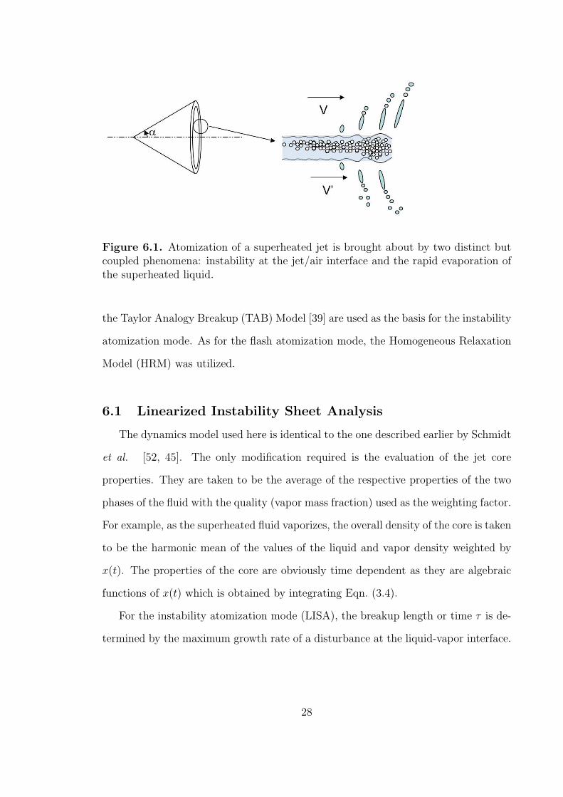
Figure 6.1. Atomization of a superheated jet is brought about by two distinct butcoupled phenomena: instability at the jet/air interface and the rapid evaporation ofthe superheated liquid.
the Taylor Analogy Breakup (TAB) Model [39] are used as the basis for the instability
atomization mode. As for the flash atomization mode, the Homogeneous Relaxation
Model (HRM) was utilized.
6.1 Linearized Instability Sheet Analysis
The dynamics model used here is identical to the one described earlier by Schmidt
et al. [52, 45]. The only modification required is the evaluation of the jet core
properties. They are taken to be the average of the respective properties of the two
phases of the fluid with the quality (vapor mass fraction) used as the weighting factor.
For example, as the superheated fluid vaporizes, the overall density of the core is taken
to be the harmonic mean of the values of the liquid and vapor density weighted by
x(t). The properties of the core are obviously time dependent as they are algebraic
functions of x(t) which is obtained by integrating Eqn. (3.4).
For the instability atomization mode (LISA), the breakup length or time τ is de-
termined by the maximum growth rate of a disturbance at the liquid-vapor interface.
28
Aerodynamic instability will atomize the core when this disturbance on the interface
grows to a critical value.
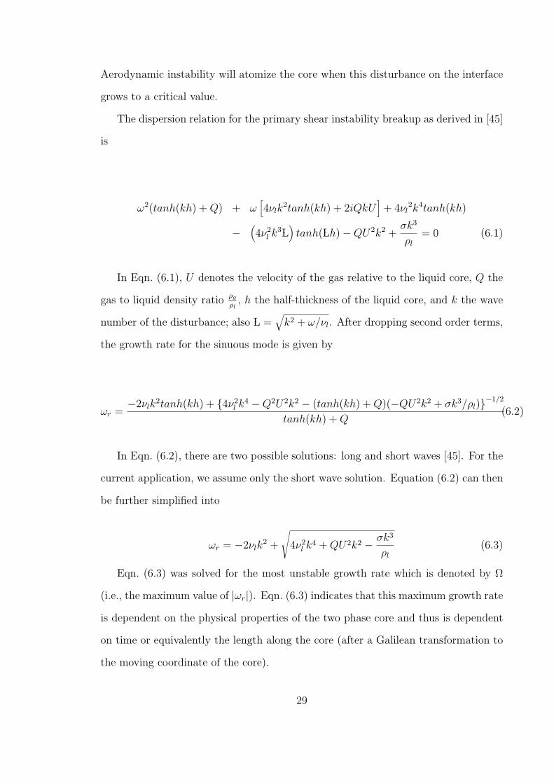
The dispersion relation for the primary shear instability breakup as derived in [45]
is
ω2(tanh(kh) +Q) + ω[
4νlk2tanh(kh) + 2iQkU
]
+ 4νl2k4tanh(kh)
−(
4ν2l k
3 L)
tanh( Lh) −QU2k2 +σk3
ρl
= 0 (6.1)
In Eqn. (6.1), U denotes the velocity of the gas relative to the liquid core, Q the
gas to liquid density ratio ρg
ρl, h the half-thickness of the liquid core, and k the wave
number of the disturbance; also L =√
k2 + ω/νl. After dropping second order terms,
the growth rate for the sinuous mode is given by
ωr =−2νlk
2tanh(kh) + 4ν2l k
4 −Q2U2k2 − (tanh(kh) +Q)(−QU2k2 + σk3/ρl)−1/2
tanh(kh) +Q(6.2)
In Eqn. (6.2), there are two possible solutions: long and short waves [45]. For the
current application, we assume only the short wave solution. Equation (6.2) can then
be further simplified into
ωr = −2νlk2 +
√
4ν2l k
4 +QU2k2 − σk3
ρl
(6.3)
Eqn. (6.3) was solved for the most unstable growth rate which is denoted by Ω
(i.e., the maximum value of |ωr|). Eqn. (6.3) indicates that this maximum growth rate
is dependent on the physical properties of the two phase core and thus is dependent
on time or equivalently the length along the core (after a Galilean transformation to
the moving coordinate of the core).
29
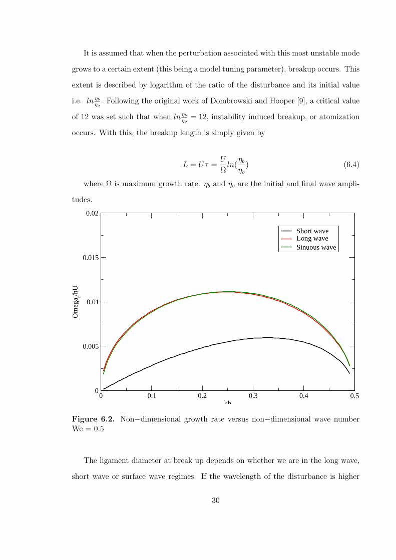
It is assumed that when the perturbation associated with this most unstable mode
grows to a certain extent (this being a model tuning parameter), breakup occurs. This
extent is described by logarithm of the ratio of the disturbance and its initial value
i.e. ln ηb
ηo. Following the original work of Dombrowski and Hooper [9], a critical value
of 12 was set such that when ln ηb
ηo= 12, instability induced breakup, or atomization
occurs. With this, the breakup length is simply given by
L = Uτ =U
Ωln(
ηb
ηo
) (6.4)
where Ω is maximum growth rate. ηb and ηo are the initial and final wave ampli-
tudes.
0 0.1 0.2 0.3 0.4 0.5kh
0
0.005
0.01
0.015
0.02
Om
ega r/h
U
Short waveLong waveSinuous wave
Figure 6.2. Non−dimensional growth rate versus non−dimensional wave numberWe = 0.5
The ligament diameter at break up depends on whether we are in the long wave,
short wave or surface wave regimes. If the wavelength of the disturbance is higher
30
0 1 2 3 4 5kh
0
0.02
0.04
0.06
0.08
0.1
Om
ega r/h
U
Short waveLong waveSinuous wave
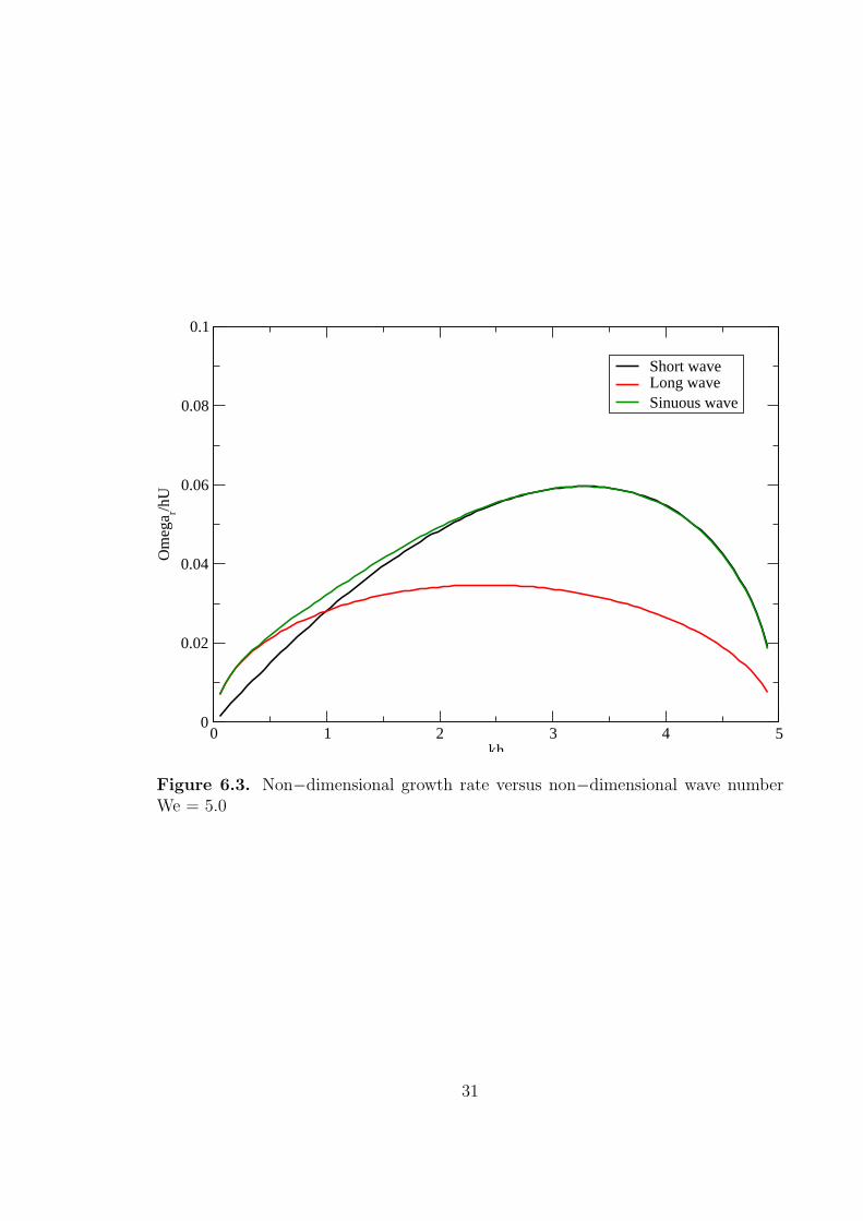
Figure 6.3. Non−dimensional growth rate versus non−dimensional wave numberWe = 5.0
31
than the half sheet thickness, it is assumed that long wave growth exists. Otherwise
short wave solution is imposed. The ligament diameter for long waves is calculated
as,
dL =
√
8h
Ks
(6.5)
where h is the half sheet thickness at breakup, Ks is the wave number of maximum
wave growth. For short waves the the ligament diameter is,
dL =
√
16h
Ks
(6.6)
If the Weber number is sufficiently high, then only surface waves exist which are
independent of the sheet thickness. The transition to surface waves in this study is
assumed to occur at a Weber number of 50. The ligament diameter of the surface
wave is assumed to be half the wavelength.
dL =π
Ks
(6.7)
The drop diameter is obtained from the ligament diameter via the following rela-
tion which is obtained by a mass balance,
d3D =
3πd2L
KL
(6.8)
Where KL is given as ,
KLdL =
(
1
2+
3µl
2√ρlσdL
)
−0.5
(6.9)
6.1.1 Derivation of Sheet Thickness
The instantaneous sinuous wave growth rate is based on the the current thickness
of the conical liquid sheet. Additionally, at breakup, the ligament diameter depends
32
upon the sheet thickness at the instance of breakup. This necessitates the computa-
tion and tracking of the sheet thickness and is done using conservation of mass. The
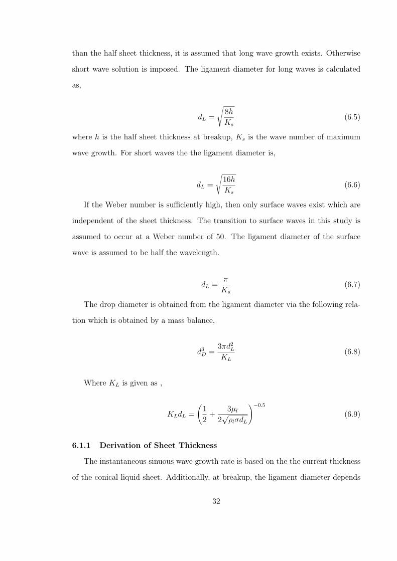
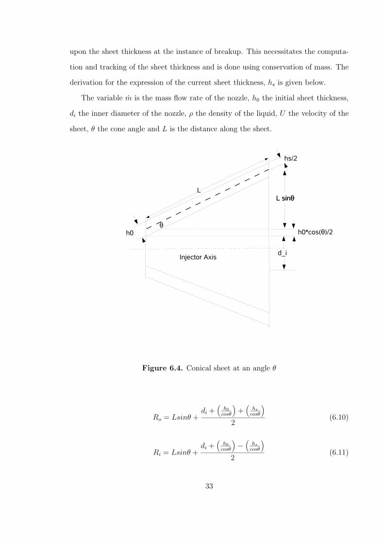
derivation for the expression of the current sheet thickness, hs is given below.
The variable m is the mass flow rate of the nozzle, h0 the initial sheet thickness,
di the inner diameter of the nozzle, ρ the density of the liquid, U the velocity of the
sheet, θ the cone angle and L is the distance along the sheet.
Figure 6.4. Conical sheet at an angle θ
Ro = Lsinθ +di +
(
h0
cosθ
)
+(
hs
cosθ
)
2(6.10)
Ri = Lsinθ +di +
(
h0
cosθ
)
−(
hs
cosθ
)
2(6.11)
33
m = ρUliqcos(θ)π((Ro)2 − (Ri)
2) (6.12)
m
ρUliqcos(θ)π= (Lsinθ +
di +(
h0
cosθ
)
+(
hs
cosθ
)
2)2 − (Lsinθ +
di +(
h0
cosθ
)
−(
hs
cosθ
)
2)2
(6.13)
m
ρUliqcos(θ)π= 2
(
hs
cosθ
)
Lsinθ +
(
h0
cosθ
)(
hs
cosθ
)
+ di
(
hs
cosθ
)
(6.14)
(
hs
cosθ
)
=m
ρUliqcos(θ)π(2Lsinθ +(
h0
cosθ
)
+ di)(6.15)
hs =m
ρUliqπ(2Lsinθ +(
h0
cosθ
)
+ di)(6.16)
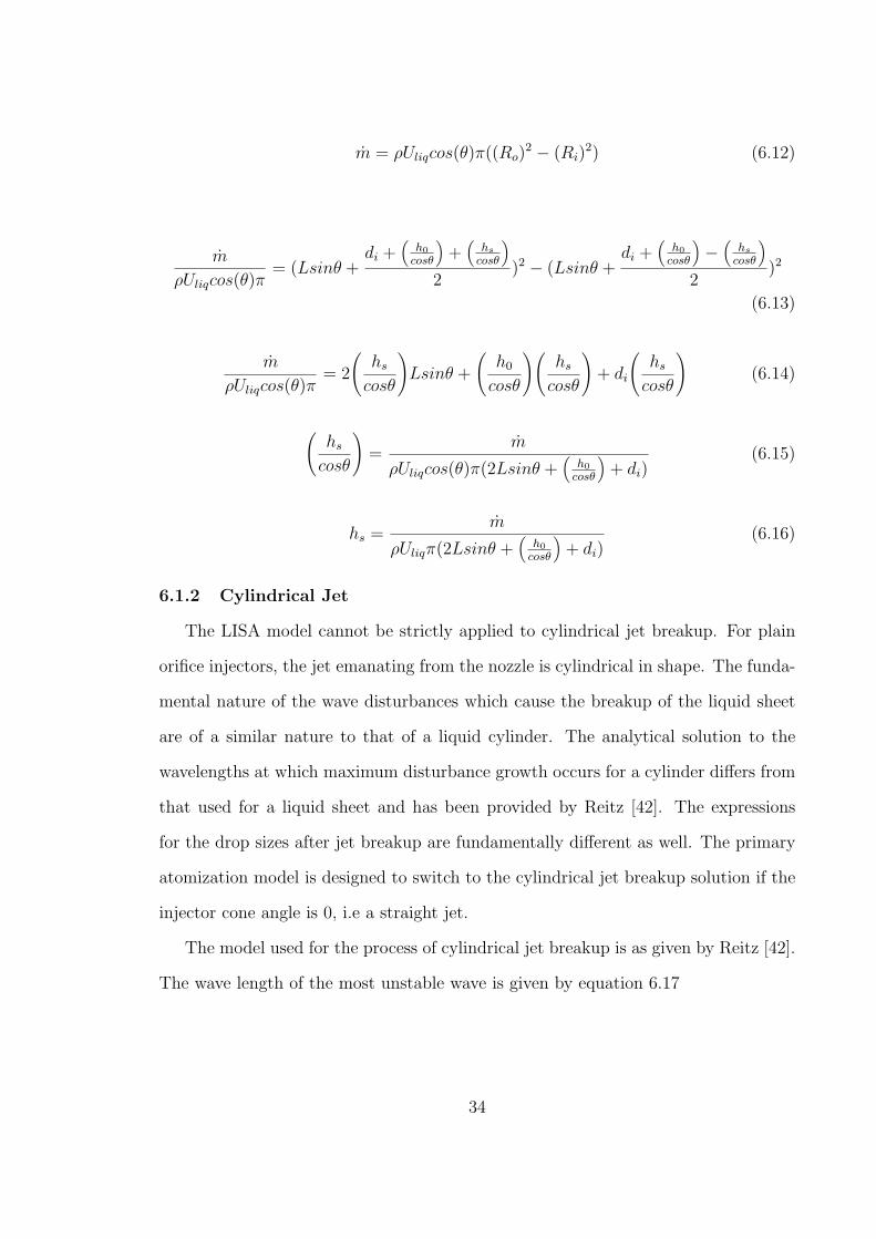
6.1.2 Cylindrical Jet
The LISA model cannot be strictly applied to cylindrical jet breakup. For plain
orifice injectors, the jet emanating from the nozzle is cylindrical in shape. The funda-
mental nature of the wave disturbances which cause the breakup of the liquid sheet
are of a similar nature to that of a liquid cylinder. The analytical solution to the
wavelengths at which maximum disturbance growth occurs for a cylinder differs from
that used for a liquid sheet and has been provided by Reitz [42]. The expressions
for the drop sizes after jet breakup are fundamentally different as well. The primary
atomization model is designed to switch to the cylindrical jet breakup solution if the
injector cone angle is 0, i.e a straight jet.
The model used for the process of cylindrical jet breakup is as given by Reitz [42].
The wave length of the most unstable wave is given by equation 6.17
34

Λ
a= 9.02
(1 + 0.45Z0.5)(1 + 0.4T 0.7)
(1 + 0.87We1.672 )0.6
(6.17)
The growth rate of the most unstable wave is equation 6.18.
Ω[ρ1a
3
σ]0.5 =
0.34 + 0.38We1.52
(1 + Z)(1 + 1.4T 0.6)(6.18)
where,
Z =We0.5
1
Re1
, T = ZWe0.52 (6.19)
We1 and Re1 are the liquid phase Weber and Reynolds number respectively. We2
is the gas phase weber number.
The breakup criterion for the jet was the same as the LISA model. The drop
radius predicted the by the model are given by equations 6.20 and 6.21. The criteria
for the switch is based on B0Λ and a. B0 is a constant assumed to be 0.61 and a is
the initial blob radius.
r = B0Λ (B0Λ ≤ a) (6.20)
r = min
(3πa2U2Ω
)0.33
(3a2Λ4
)0.33
(B0Λ > a) (6.21)
For the primary atomization model, the Homogeneous Relaxation Model (HRM)
is coupled with the sheet atomization model (LISA) and the cylindrical jet breakup
model (Reitz). The thermodynamic relaxation process competes with instability
growth model in a race to achieve the breakup criterion.
35
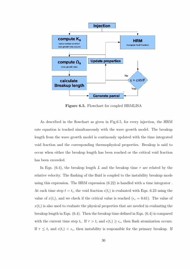
Figure 6.5. Flowchart for coupled HRMLISA
As described in the flowchart as given in Fig.6.5, for every injection, the HRM
rate equation is tracked simultaneously with the wave growth model. The breakup
length from the wave growth model is continously updated with the time integrated
void fraction and the corresponding thermophysical properties. Breakup is said to
occur when either the breakup length has been reached or the critical void fraction
has been exceeded.
In Eqn. (6.4), the breakup length L and the breakup time τ are related by the
relative velocity. The flashing of the fluid is coupled to the instability breakup mode
using this expression. The HRM expression (6.22) is handled with a time integrator .
At each time step t = ti, the void fraction ǫ(ti) is evaluated with Eqn. 6.23 using the
value of x(ti), and we check if the critical value is reached (ǫc = 0.61). The value of
x(ti) is also used to evaluate the physical properties that are needed in evaluating the
breakup length in Eqn. (6.4). Then the breakup time defined in Eqn. (6.4) is compared
with the current time step ti. If τ > ti and ǫ(ti) ≥ ǫc, then flash atomization occurs.
If τ ≤ ti and ǫ(ti) < ǫc, then instability is responsible for the primary breakup. If
36
none of these two conditions are met, the time integration continues. Depending on
which physical phenomenon is responsible for the primary breakup, the appropriate
submodel that describes the droplet number density will be used.
When this breakup time is shorter then the time required for the superheated
liquid to reach the critical void fraction, the instability breakup mode takes over the
atomization process. If flashing reaches its critical condition sooner, then, it becomes
the atomization mechanism. For the flash atomization mode, the breakup criteria is
the critical void fraction. Senda et al. [51] and Kawano et al. [26], in their work on
superheated gasoline, discovered that the primary core flash atomization occurs when
the void fraction (vapor volume fraction) reaches a value of 0.61 ca. In a related work
of Zeng and Lee [67], a more elaborate model for an isolated superheated droplet also
yielded a similar criticality condition for a wide range of conditions. Sher and Elata
[53], who worked on aerosols, concluded that this critical void fraction is related to
the packing limit of spheres in a volume i.e. the maximum number of identical spheres
that can be packed in a given volume [5]. There are many theories on the evaluation
of this packing limit, but in three dimensions they all predict a volume ratio of
approximately in the range of 0.6 to 0.7. The physical reasoning of this criticality
is obvious: when the core cannot accommodate any more bubbles, it shatters - the
geometry changes from “bubbles-in-liquid” to “droplets-in-vapor”.
The dual mode model as described, mathematically, is formulated in the following
way. First we construct the model that describes the time variation of the void
fraction using the HRM by combining equations (3.4) and (6.23). These, together
with the critical void fraction as the break up criteria, complete the main part of the
flash atomization component. What remains is the model that describes the droplet
number density subsequent to the flash atomization process which is discussed in the
next section. Note that the same flash atomization model is used in both the primary
and the secondary breakup processes.
37

6.2 Homogenous Relaxation Model
The non−equilibrium phase change process is tracked by the Homogenous Relax-
ation Model [10] . The rate of vapor formation is given by,
dx
dt=xeq − x
Θ; Θ = Θoǫ
αφβ; α = −0.54; β = −1.76; Θo = 6.51e−4[s] (6.22)
where in xeq(p, h) denotes the equilibrium quality; α, β, and Θo are model con-
stants. ǫ and φ denote, respectively, the void fraction and the degree of superheat of
the system.
ǫ =ρl − ρ
ρl − ρv
; φ =Pb(h) − P
Pc − Pb(h)(6.23)
Pc is the critical pressure of the fluid. Pb(h) is the bubble point pressure of the
system for the particular enthalpy. The void fraction is tracked along with the HRM
rate equation. The sheet is assumed to breakup when the void fraction reaches a
critical value of 0.6.
Figure 6.6. Bubble growth and subsequent breakup into droplets
38
The number of nucleation sites for bubbles is obtained from a relation provided
by Senda et al [51]. The nucleation density is a function of the degree of superheat
of the fluid which is denoted as δθ.
N = C · e−5.279d0/δθ (6.24)
The constant C is assumed to have a value of 5.757 ∗ 1012 as reported by Senda
et al [51]. The droplet diameter for flash induced breakup is purely based on thermo-
dynamic quantities and is given as,
D = 2 · (1 − ǫ83πN
)1/3 (6.25)
where ǫ is the void fraction. It is assumed that for every bubble two daughter
droplets will be formed as given by Senda et al[51].
6.3 Taylor Analogy Breakup
The secondary breakup model was constructed similarly to the primary atom-
ization model. The Taylor Analogy Breakup (TAB) model [39] and the HRM were
combined. The TAB model describes the perturbation of a droplet from its initial
spherical shape using a single parameter y, which denotes the deformation of the
single droplet.
ρlR3y = CF/CbρgU
2R− CKσy − CdµlyR (6.26)
In Eqn. (6.26), U denotes the droplet velocity relative to the ambient, R the
droplet radius, y the normalized droplet shape perturbation, σ the surface tension,
µl the viscosity of the two-phase fluid within the droplet, ρl the density of the two-
phase fluid within the droplet, and ρg the density of the ambient gas. CF , Cb, CK ,
and Cd are modeling parameters with values of 1/3, 1/2, 8, and 5 respectively, as
39

given by O’rourke [39]. Equation (6.26) is then integrated in time simultaneously
with the HRM model i.e., equations (6.22) and (6.23). The breakup criteria for
the TAB model was taken to be y = 1 [39] and the same criticality criteria for the
flash atomization mode as described before was utilized for the secondary breakup
model. Again, the physical process that reaches its critical condition first will be the
controlling mechanism. The flowchart for the coupled secondary breakup process is
given in Fig.6.7.
Figure 6.7. Flowchart for coupled HRMTAB
If flash atomization occurs, the same procedure used in the primary breakup
model to obtain the droplet number density was implemented here. If TAB is the
breakup mechanism, the expression developed in [39] for the mean droplet radius was
implemented.
rs =rinit
1 + 43∗ y2 +
ρr3
init
8σ(y)2
(6.27)
40

CHAPTER 7
INTERNAL NOZZLE FLOW - RESULTS AND
VALIDATION
All the test cases used for validation were channel flows containing water. Though
the simulation is transient, the experiments were always steady state, so all calcula-
tions were run until both the inflow and outflow had stabilized. The typical flash-
boiling experiment is a straight channel with a sharp inlet. The sharp corner creates
the potential for a separated flow with strong two-dimensional flow features. For con-
venience, these kinds of flows were simulated as axisymmetric flow. To avoid imposing
boundary conditions where sharp gradients would be present, a plenum was added to
both the inlet and outlet side of the channel, as shown in Fig. 7.1. The addition of the
plenum provides some separation distance between the imposed boundary conditions
and the region of interest. An unstructured quadrilateral mesh was used throughout
the whole domain.
Figure 7.1. A typical two-dimensional computational domain.
41

7.1 Reitz Experiment
An experimental investigation using an axisymmetric nozzle and water as the
working fluid was done by Reitz [43]. The downstream pressure was kept at 101
kPa and the inlet pressure was fixed at 787 kPa. He varied the inlet temperature
and noted the effect on mass flow rate. The mass flow rate gradually decreased
until an upstream temperature of about 430K was reached, whereupon the mass flow
discontinuously dropped. Reitz reported that the mass flow rate dropped below the
measurement range of his flow meter.
This experiment was simulated for validation and to provide new knowledge not
obtainable in the original measurements. In the simulation, the axisymmetry of the
nozzle was exploited to achieve quicker results. Fig.7.2 shows the geometry of the
nozzle used in both the experiment and in the simulations.
Figure 7.2. Nozzle design used by Reitz[43]. All dimensions are in centimeters.
42
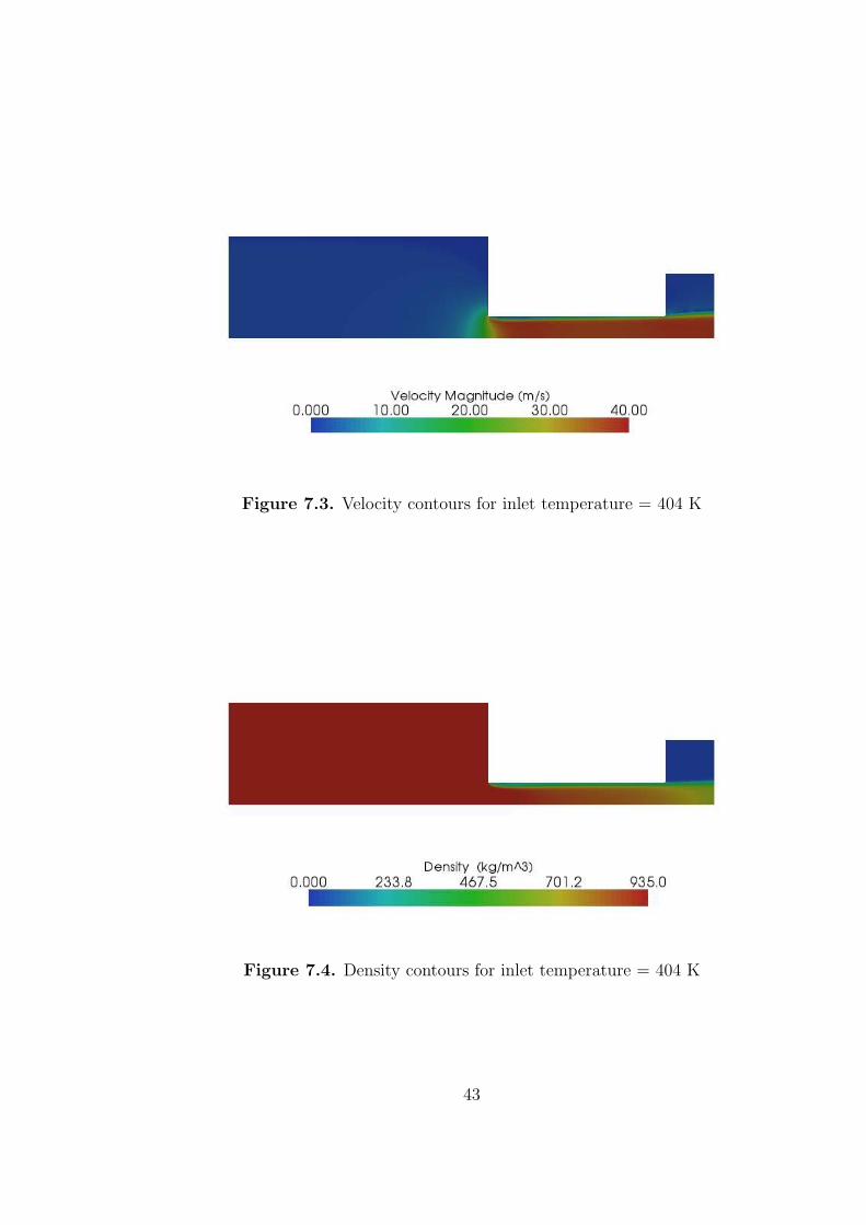
Figure 7.3. Velocity contours for inlet temperature = 404 K
Figure 7.4. Density contours for inlet temperature = 404 K
43
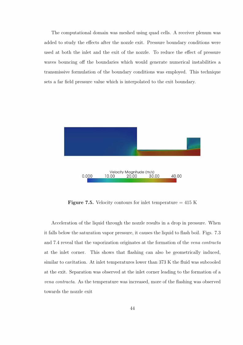
The computational domain was meshed using quad cells. A receiver plenum was
added to study the effects after the nozzle exit. Pressure boundary conditions were
used at both the inlet and the exit of the nozzle. To reduce the effect of pressure
waves bouncing off the boundaries which would generate numerical instabilities a
transmissive formulation of the boundary conditions was employed. This technique
sets a far field pressure value which is interpolated to the exit boundary.
Figure 7.5. Velocity contours for inlet temperature = 415 K
Acceleration of the liquid through the nozzle results in a drop in pressure. When
it falls below the saturation vapor pressure, it causes the liquid to flash boil. Figs. 7.3
and 7.4 reveal that the vaporization originates at the formation of the vena contracta
at the inlet corner. This shows that flashing can also be geometrically induced,
similar to cavitation. At inlet temperatures lower than 373 K the fluid was subcooled
at the exit. Separation was observed at the inlet corner leading to the formation of a
vena contracta. As the temperature was increased, more of the flashing was observed
towards the nozzle exit
44
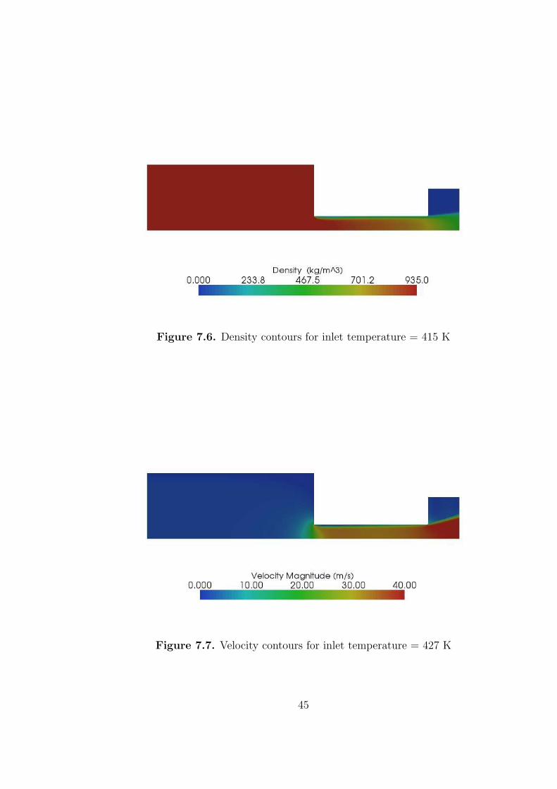
Figure 7.6. Density contours for inlet temperature = 415 K
Figure 7.7. Velocity contours for inlet temperature = 427 K
45

Figure 7.8. Density contours for inlet temperature = 427 K
With increased inlet temperature, the rate of flashing increases within the nozzle.
This is is noted by the reduction in density in the contour plots, Figs. 7.4, 7.6, 7.8
and 7.10. The higher quantity of vapor in the interior of the nozzle causes a decrease
in the overall mass flow rate of the fluid. Also, as the jet exits the nozzle, rapid
expansion takes place as the vapor is no longer constrained by the nozzle wall.
Experiments with sprays undergoing flash atomization [66, 1] have observed an
increase in the spray cone angle with the rise in the temperature of the working fluid.
The contour plots of velocity in Figs. 7.3, 7.5, 7.7, and 7.9 show that fluid ejects
at wider angles successively as the inlet enthalpy increases while the vena contracta
undergoes little change..
The further increase in the temperature of the fluid promotes vaporization to such
an extent that the liquid completely vaporizes inside the nozzle resulting in a dramatic
decrease of the mass flow rate and a condition of “vapor lock.” Though the exper-
imental data show the approximate temperature where this discontinuous reduction
46

Figure 7.9. Velocity contours for inlet temperature = 438 K
Figure 7.10. Density contours for inlet temperature = 438 K
47
of mass flow occurred, the actual mass flow rate dropped below the resolution of the
flow meter at about 430K. A comparison of the computed and measured mass flow
rates is given in Fig. 7.11. An analytical calculation based on Bernoulli’s equation
will grossly overpredict the mass flow rate. Even frozen flow models will under pre-
dict vapor formation thus leading to erroneous results. The frozen flow calculations
reported are achieved by setting the timescale of vaporization to a sufficiently high
value compared to the characteristic time of the system. For practical purposes the
phase change time can be considered infinite in the frozen flow calculations. On the
other end of the spectrum, an equation of state approach is achieved by setting the
timescale of vaporization to a value smaller than the timestep size of the computation.
This method results in excessive vapor generation and hence a much lower prediction
of mass flow rates.
An equilibrium type calculation at higher temperatures poses additional numerical
challenges as well. For example, consider the case for which the inlet temperature of
the incoming fluid is 438 K. The equilibrium vapor density at this temperature is
0.5 kg/m3. Assuming a nozzle discharge coefficient of 0.6, an analytical calculation
gives that the predicted velocity of the vapor at the exit is 993.9 m/s. This value of
exit velocity is not only unrealistic but will also be a large source of numerical error
in any computation.
The finite rate process modeled by HRM is shown to obtain results very close to
that experimentally observed. Though there is slight disagreement about the exact
temperature at which the drop-off in flow occurs, the model succeeds in predicting the
mass flow rate in the flashing nozzle over a range of temperature. In the simulations,
the critical temperature for vapor lock corresponds closely to the temperature at which
the vapor pressure equals the upstream static pressure. At the upstream pressure of
787 kPa, the saturation temperature of water is 443 K. Under superheated conditions,
48
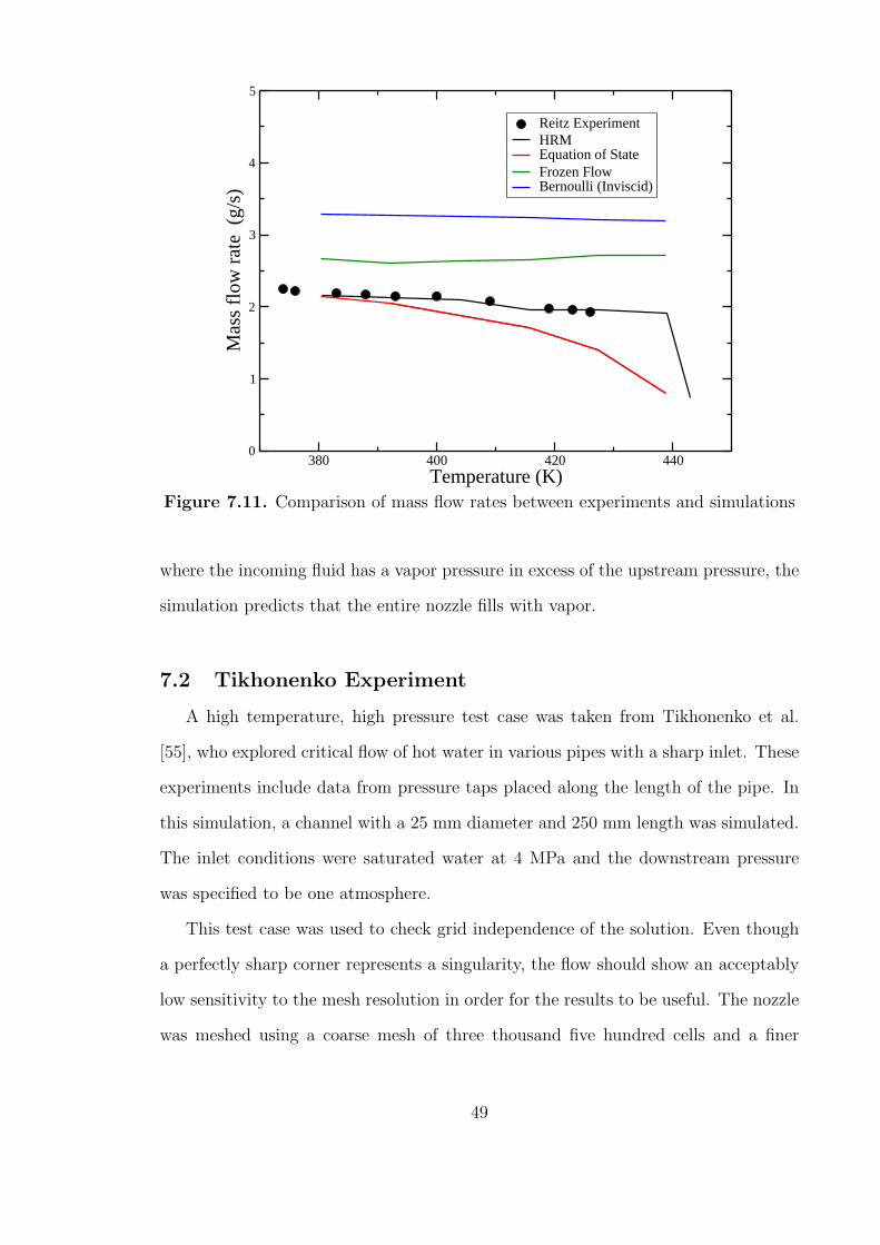
380 400 420 440Temperature (K)
0
1
2
3
4
5
Mas
s fl
ow r
ate
(g/
s)
Reitz ExperimentHRMEquation of StateFrozen FlowBernoulli (Inviscid)
Figure 7.11. Comparison of mass flow rates between experiments and simulations
where the incoming fluid has a vapor pressure in excess of the upstream pressure, the
simulation predicts that the entire nozzle fills with vapor.
7.2 Tikhonenko Experiment
A high temperature, high pressure test case was taken from Tikhonenko et al.
[55], who explored critical flow of hot water in various pipes with a sharp inlet. These
experiments include data from pressure taps placed along the length of the pipe. In
this simulation, a channel with a 25 mm diameter and 250 mm length was simulated.
The inlet conditions were saturated water at 4 MPa and the downstream pressure
was specified to be one atmosphere.
This test case was used to check grid independence of the solution. Even though
a perfectly sharp corner represents a singularity, the flow should show an acceptably
low sensitivity to the mesh resolution in order for the results to be useful. The nozzle
was meshed using a coarse mesh of three thousand five hundred cells and a finer
49

mesh with fifteen thousand cells. A comparison of predicted wall pressures from the
several calculations, exploring both the high pressure and low pressure correlations
(see Eqns. 3.8 and 3.10) and mesh sensitivity, can be seen in Fig. 7.12. The coarser
mesh is sufficiently close to the fine mesh result, such that the modeling assumptions
are a larger source of error than the discretization error.
The results for static pressure along the pipe wall in Fig. 7.12 also permit a
comparison of the two correlations, as well as revealing some of the internal flow
features. The experimentally-measured pressure shows a slight local minimum near
the inlet corner due to the separated flow. As the computational results will show, the
liquid forms a vena contracta downstream of the inlet. Once past the vena contracta,
the pressure partially recovers and then drops precipitously at the exit.
The computational results follow the expected trend. There is a local pressure
minimum on the wall just downstream of the inlet corner in the simulations. The
pressure recovers slightly and then remains nearly constant along the nozzle length
until just upstream of the nozzle exit. The pressure at the nozzle exit decreases
dramatically due to rapid flashing near the exit plane. However, both correlations
under-predict the rate of flash boiling, though the low pressure correlation is especially
far off. The high pressure correlation produces pressures that are much closer to the
experimental measurements.
In addition to predicting pressure, the computational results show other features
of interest, such as pressure, velocity, density, and the rate of change of quality. These
results can be used to explain the nozzle behavior under these flow conditions.
As in both single-phase and cavitating nozzles, the flow separates off of the sharp
inlet corner [44]. In an incompressible flow, the pressure would be expected to be
extremely low downstream of this corner, due to the separated flow and the constraint
of a divergence-free velocity field. However, with flashing flow, the decrease in pressure
creates an increase in the rate of phase change. The flashing of the liquid creates a
50

0 2 4 6 8 10x/D
0
0.1
0.2
0.3
0.4
0.5
0.6
0.7
0.8
0.9
1
p/p 0
ExperimentCoarse Mesh - incompressible -High pressure correlationFine Mesh - incompressible -High pressure correlationCoarse mesh - incompressible - Low pressure correlationFine Mesh - incompressible - Low pressure correlationCompressible - Low pressure correlation
Figure 7.12. Static pressure versus position at the wall for saturated water at 4MPa discharging through a 25 mm tube with L/D=10
51
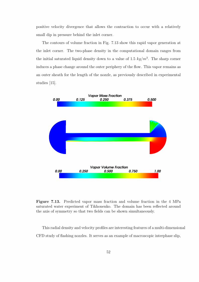
positive velocity divergence that allows the contraction to occur with a relatively
small dip in pressure behind the inlet corner.
The contours of volume fraction in Fig. 7.13 show this rapid vapor generation at
the inlet corner. The two-phase density in the computational domain ranges from
the initial saturated liquid density down to a value of 1.5 kg/m3. The sharp corner
induces a phase change around the outer periphery of the flow. This vapor remains as
an outer sheath for the length of the nozzle, as previously described in experimental
studies [15].
Figure 7.13. Predicted vapor mass fraction and volume fraction in the 4 MPasaturated water experiment of Tikhonenko. The domain has been reflected aroundthe axis of symmetry so that two fields can be shown simultaneously.
This radial density and velocity profiles are interesting features of a multi-dimensional
CFD study of flashing nozzles. It serves as an example of macroscopic interphase slip,
52
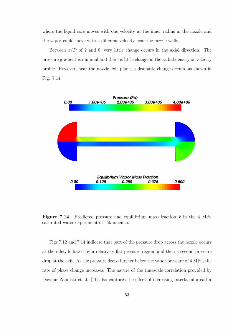
where the liquid core moves with one velocity at the inner radius in the nozzle and
the vapor could move with a different velocity near the nozzle walls.
Between x/D of 2 and 8, very little change occurs in the axial direction. The
pressure gradient is minimal and there is little change in the radial density or velocity
profile. However, near the nozzle exit plane, a dramatic change occurs, as shown in
Fig. 7.14.
Figure 7.14. Predicted pressure and equilibrium mass fraction x in the 4 MPasaturated water experiment of Tikhonenko.
Figs.7.12 and 7.14 indicate that part of the pressure drop across the nozzle occurs
at the inlet, followed by a relatively flat pressure region, and then a second pressure
drop at the exit. As the pressure drops further below the vapor pressure of 4 MPa, the
rate of phase change increases. The nature of the timescale correlation provided by
Downar-Zapolski et al. [11] also captures the effect of increasing interfacial area for
53

phase change, due to the dependence on vapor volume fraction. So, with the creation
of vapor, the rate of phase change is further increased. Note how the timescale shown
in Fig. 7.15 correlates with the creation of vapor. By conservation of mass, the drop
in density is accompanied by an increase in axial velocity. Conservation of momentum
then indicates that pressure drops further. This pressure drop, in turn, feeds back
into the flashing process. The pressure finally reaches the downstream value just
outside of the nozzle.
Figure 7.15. Predicted velocity magnitude and the common log of the phase changetimescale Θ for the 4 MPa saturated water experiment of Tikhonenko.
The anticipation that the flashing flow process would continue just beyond the
nozzle motivated the decision to place the computational boundary downstream of
the nozzle. However, the model does not account for the presence of non-condensible
gases, such as air. Fortunately for this case, it appears from the velocity field that air
54
is not entrained into the internal nozzle flow. The strong favorable pressure gradient
near the nozzle exit discourages the counter-flow of air and produces no recirculating
flow in the exit plenum of the computational domain.
The ability of the model to predict choking was also investigated. The high liquid
temperature and low downstream pressure suggests that the flow should be choked
[17]. Computationally, this is indeed the case. The above simulation was re-run with
the downstream pressure set to two atmospheres, which reduces the pressure drop
across the nozzle by 2.6 percent. The computed mass flow rate changed by less than
0.03 percent.
7.3 Fauske Experiment
The second test case was chosen to emphasize two-dimensional effects. In these
experiments Fauske [17] studied saturated water discharge through short tubes. He
noted the maximum discharge rates as a function of L/D and upstream stagnation
pressure. Of the various nozzles that Fauske tested, a relatively short nozzle was
chosen for validation, with L/D = 4, in the next test case. It is expected that the
inlet corners will cause large variations of void fraction and velocity in the radial
direction. These two-dimensional effects are likely to be more pronounced than in
the longer nozzle discussed above.
First, the mass flow rates were compared for 6.35 mm diameter tubes at stagnation
pressures of 1.37 MPa, 4.13 MPa, and 6.89 MPa. The calculated mass flow rates using
the low-pressure correlation, Eq. 3.8 are compared to Fauske’s measurements in Fig.
7.16. The agreement of the data is excellent, with the computed results lying within
the scatter of the experimental data. The good agreement produced by the low-
pressure correlation is somewhat surprising and much better than the high-pressure
correlation, Eq. 3.10, which under-predicted mass flow rate by a factor of two.
55
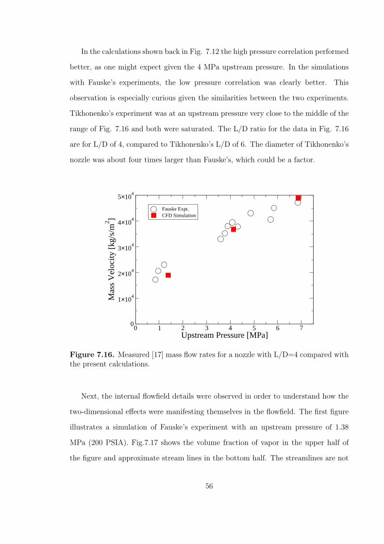
In the calculations shown back in Fig. 7.12 the high pressure correlation performed
better, as one might expect given the 4 MPa upstream pressure. In the simulations
with Fauske’s experiments, the low pressure correlation was clearly better. This
observation is especially curious given the similarities between the two experiments.
Tikhonenko’s experiment was at an upstream pressure very close to the middle of the
range of Fig. 7.16 and both were saturated. The L/D ratio for the data in Fig. 7.16
are for L/D of 4, compared to Tikhonenko’s L/D of 6. The diameter of Tikhonenko’s
nozzle was about four times larger than Fauske’s, which could be a factor.
0 1 2 3 4 5 6 7Upstream Pressure [MPa]
0
1×10⁴
2×10⁴
3×10⁴
4×10⁴
5×10⁴
Mas
s V
eloc
ity [
kg/s
/m2 ]
Fauske Expt.CFD Simulation
Figure 7.16. Measured [17] mass flow rates for a nozzle with L/D=4 compared withthe present calculations.
Next, the internal flowfield details were observed in order to understand how the
two-dimensional effects were manifesting themselves in the flowfield. The first figure
illustrates a simulation of Fauske’s experiment with an upstream pressure of 1.38
MPa (200 PSIA). Fig.7.17 shows the volume fraction of vapor in the upper half of
the figure and approximate stream lines in the bottom half. The streamlines are not
56
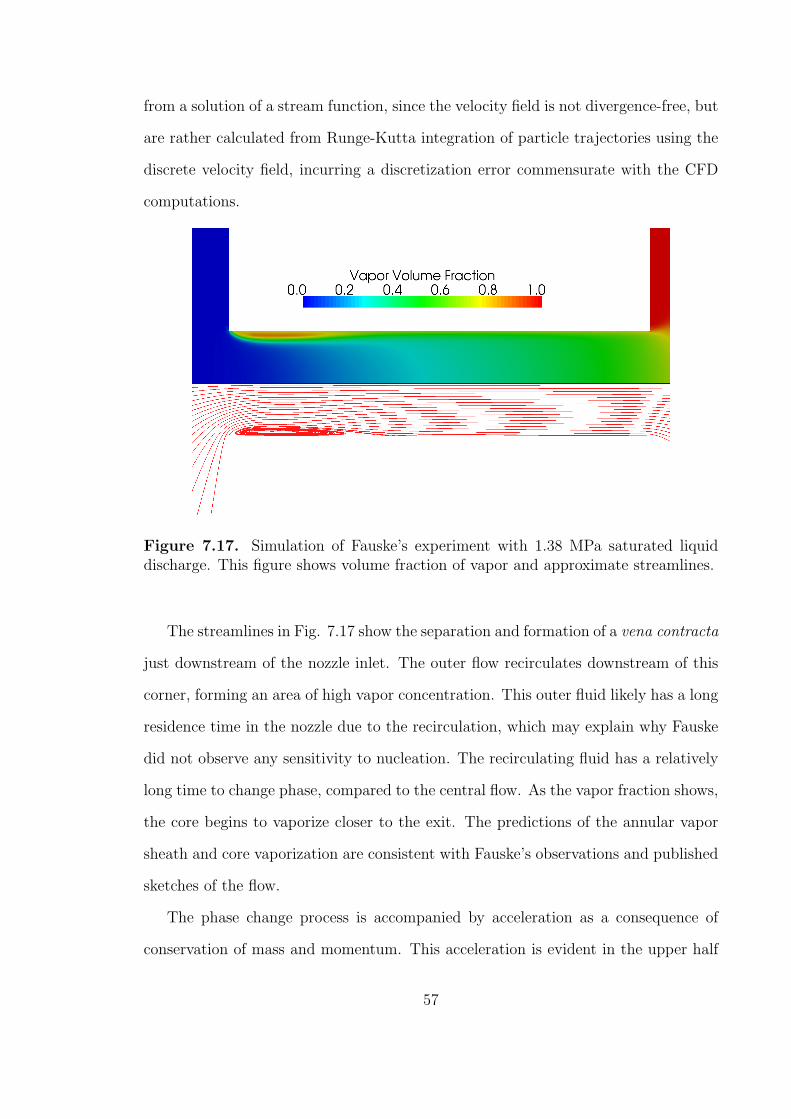
from a solution of a stream function, since the velocity field is not divergence-free, but
are rather calculated from Runge-Kutta integration of particle trajectories using the
discrete velocity field, incurring a discretization error commensurate with the CFD
computations.
Figure 7.17. Simulation of Fauske’s experiment with 1.38 MPa saturated liquiddischarge. This figure shows volume fraction of vapor and approximate streamlines.
The streamlines in Fig. 7.17 show the separation and formation of a vena contracta
just downstream of the nozzle inlet. The outer flow recirculates downstream of this
corner, forming an area of high vapor concentration. This outer fluid likely has a long
residence time in the nozzle due to the recirculation, which may explain why Fauske
did not observe any sensitivity to nucleation. The recirculating fluid has a relatively
long time to change phase, compared to the central flow. As the vapor fraction shows,
the core begins to vaporize closer to the exit. The predictions of the annular vapor
sheath and core vaporization are consistent with Fauske’s observations and published
sketches of the flow.
The phase change process is accompanied by acceleration as a consequence of
conservation of mass and momentum. This acceleration is evident in the upper half
57

Figure 7.18. Simulation of Fauske’s experiment with 1.38 MPa saturated liquiddischarge. This figure shows velocity magnitude and the common logarithm of thetimescale of phase change.
of Fig. 7.18. The initial contraction near the throat of the vena contracta produces
an acceleration as the core flow passes through a reduced cross-sectional area in the
nozzle. A second acceleration occurs near the exit, where vapor is formed.
As vapor is formed, more interfacial area is available for heat transfer, which feeds
back into the phase change process by shortening the timescale. The feedback of
between interfacial area and the timescale can be seen in the lower half of 7.18, where
the lowest values of the timescale represent regions where the fluid will move more
quickly towards the equilibrium quality.
The above figures were only considering the lower end of the range of upstream
pressures. However, the general character of the nozzle flow in these saturated dis-
charge calculations is relatively insensitive to variations in the upstream pressure.
Though velocities increase with increasing upstream pressure, the vena contracta re-
mains a relatively constant feature. The amount of vapor does not change much with
a factor of five increase in upstream saturation pressure, as shown in Fig. 7.19. The
58
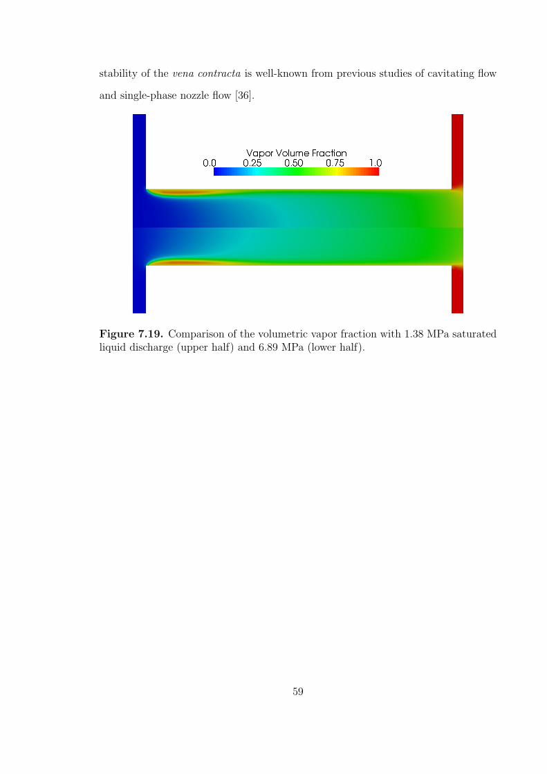
stability of the vena contracta is well-known from previous studies of cavitating flow
and single-phase nozzle flow [36].
Figure 7.19. Comparison of the volumetric vapor fraction with 1.38 MPa saturatedliquid discharge (upper half) and 6.89 MPa (lower half).
59

7.4 Three Dimensional Nozzle
Simulations were performed on a three dimensional, single-hole, asymmetric fuel
injector shown in Fig. 7.21. The design for the fuel injector obtained from Bosch
GmbH is shown in Fig.7.20. This particular design is intended for research only and
not for production purposes. The single nozzle is offset at an angle such that the
entry of the fuel was non−orthogonal. A receiver plenum has been added for this
case as well to capture physics downstream of the nozzle exit.
Figure 7.20. Orthographic projection of the injector design obtained from BoschGmbH.
A hybrid mesh is employed with hexahedral cells in the nozzle interior (see Fig.
7.22) and tetrahedral cells in the rest of the injector volume, for a total cell count of
two-hundred thirty-eight thousand. A Dirichlet pressure condition was specified at
the exit of the nozzle and it was set to 1 bar for all the cases. A time-varying velocity
condition was specified at the inlet in which the velocity was ramped up to a final
steady-state velocity over a time 0.1 ms. Table 1 provides the boundary conditions
60
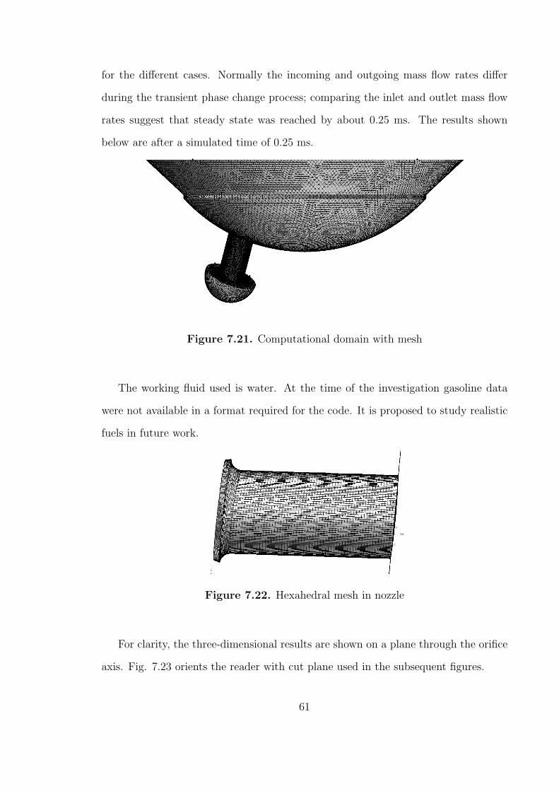
for the different cases. Normally the incoming and outgoing mass flow rates differ
during the transient phase change process; comparing the inlet and outlet mass flow
rates suggest that steady state was reached by about 0.25 ms. The results shown
below are after a simulated time of 0.25 ms.
Figure 7.21. Computational domain with mesh
The working fluid used is water. At the time of the investigation gasoline data
were not available in a format required for the code. It is proposed to study realistic
fuels in future work.
Figure 7.22. Hexahedral mesh in nozzle
For clarity, the three-dimensional results are shown on a plane through the orifice
axis. Fig. 7.23 orients the reader with cut plane used in the subsequent figures.
61
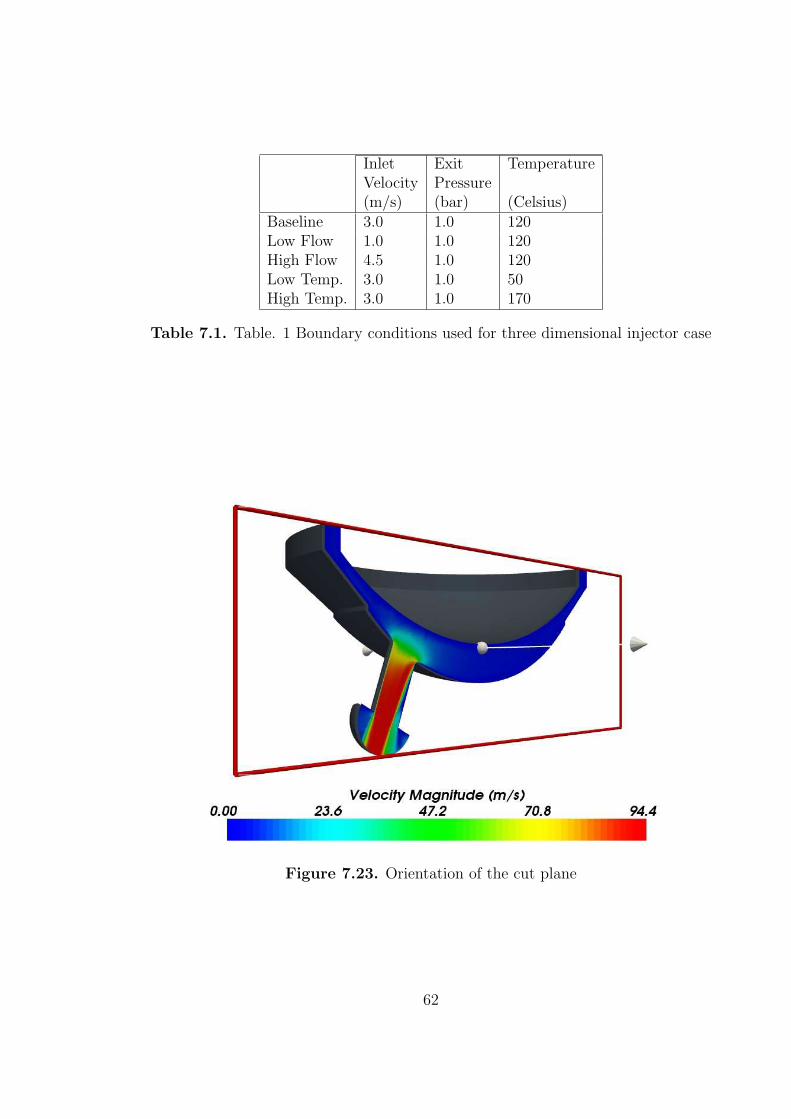
Inlet Exit TemperatureVelocity Pressure(m/s) (bar) (Celsius)
Baseline 3.0 1.0 120Low Flow 1.0 1.0 120High Flow 4.5 1.0 120Low Temp. 3.0 1.0 50High Temp. 3.0 1.0 170
Table 7.1. Table. 1 Boundary conditions used for three dimensional injector case
Figure 7.23. Orientation of the cut plane
62
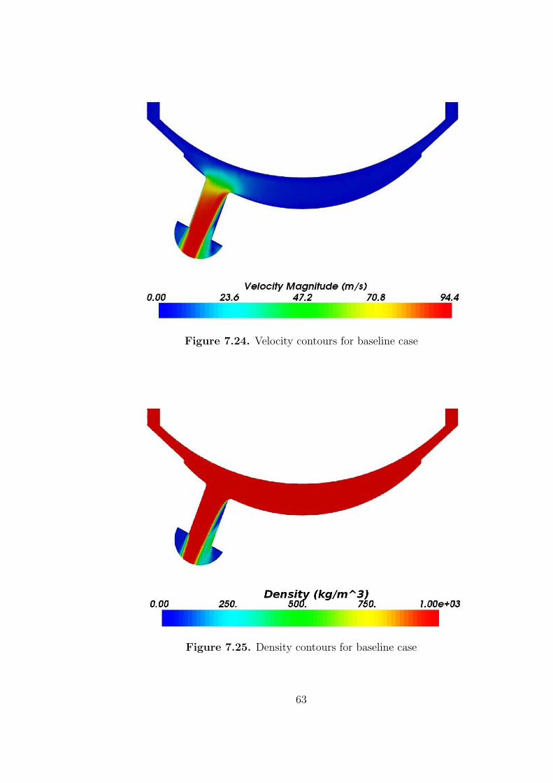
Figure 7.24. Velocity contours for baseline case
Figure 7.25. Density contours for baseline case
63

Similar to the axisymmetric nozzle, it is noted that flashing begins at the inlet
corner. The asymmetry of the nozzle design induces vapor formation at the corner
which is closer to the central axis of the injector, as is depicted in Figs. 7.24 and 7.25.
This also forces the jet exiting the nozzle to be non-uniform and the liquid core to be
shifted outward.
Figure 7.26. Velocity contours for low flow case
For the low flow case, it is observed that vaporization is diminished and the liquid
core is more prominent, as can been seen in Figs. 7.26 and 7.27. The high flow case,
shown in Figs.7.28 and 7.29, has significantly more vapor formation as compared to
the baseline and low flow cases. The expansion of the jet as it exits the nozzle is also
at a much wider angle in comparison to the previous two cases.
Lowering the temperature changes the pattern of the vapor formation as seen
in Fig. 7.31. The spread of the vapor compared to baseline case is narrower with
vapor at the widest part having a lower density. On the other hand, increasing the
64

Figure 7.27. Density contours for low flow case
Figure 7.28. Velocity contours for high flow case
65

Figure 7.29. Density contours for high flow case
Figure 7.30. Velocity contours for low temperature case
66
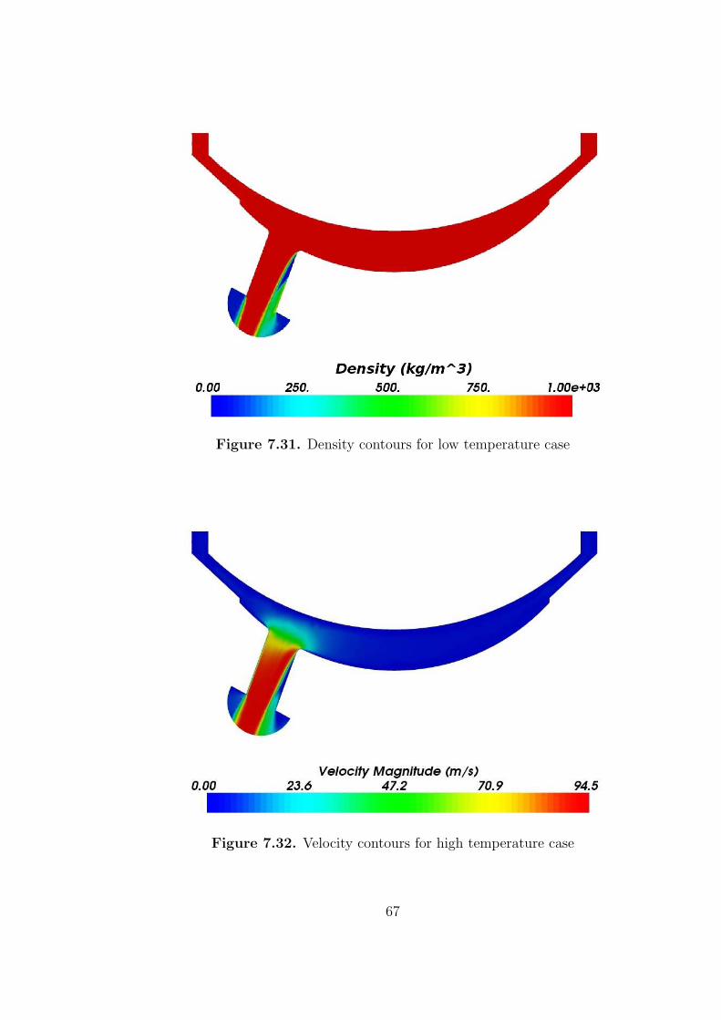
Figure 7.31. Density contours for low temperature case
Figure 7.32. Velocity contours for high temperature case
67
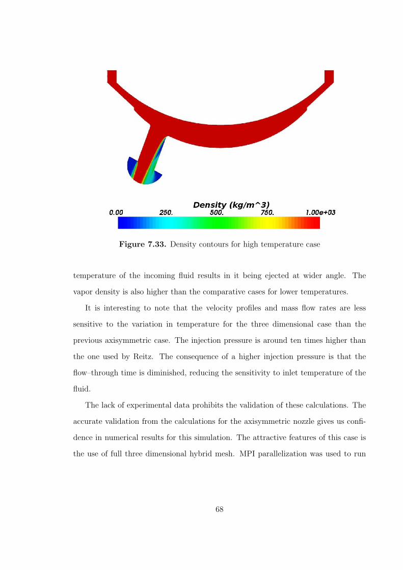
Figure 7.33. Density contours for high temperature case
temperature of the incoming fluid results in it being ejected at wider angle. The
vapor density is also higher than the comparative cases for lower temperatures.
It is interesting to note that the velocity profiles and mass flow rates are less
sensitive to the variation in temperature for the three dimensional case than the
previous axisymmetric case. The injection pressure is around ten times higher than
the one used by Reitz. The consequence of a higher injection pressure is that the
flow–through time is diminished, reducing the sensitivity to inlet temperature of the
fluid.
The lack of experimental data prohibits the validation of these calculations. The
accurate validation from the calculations for the axisymmetric nozzle gives us confi-
dence in numerical results for this simulation. The attractive features of this case is
the use of full three dimensional hybrid mesh. MPI parallelization was used to run
68

the case on multiple processors. Speedup tests indicated super-linear performance
enhancement using up to six processors on a cluster of dual-CPU Itaniums.
7.5 Conclusions
The first major finding of this work is that the flashing begins well inside the
nozzle, typically near the inlet corner. The phase change process is usually geometri-
cally induced, similar to cavitation. Unlike cavitation, the vapor region continues to
expand as the flow proceeds towards the exit.
The second finding is that at high temperatures the phase change process begins
to manifest itself strongly across the breadth of the nozzle exit. The outer sheath
of vapor is supplemented by vapor created across the entire exit plane. Further,
at the highest temperatures a strong radial expansion of the flow is evident in the
computational results, which is consistent with expectations that the flashing flow
should produce a wider spray angle.
The final observations are from the three-dimensional calculations. These cal-
culations show asymmetric vapor generation due to the angle between the nozzle
and the tip volume. The simulations were performed with higher injection pressures
than those used in the two-dimensional experimental validation cases. Because of the
shorter flow-through time and the stronger inertia of the flow, there is less sensitivity
of the internal nozzle flow to the fluid temperature. This observation of the internal
flow should not lead the reader to assume that the exterior spray will be less sensitive
to temperature.
69

CHAPTER 8
INTERNAL FLASHING FLOW OF JP8
The internal flow model was coupled to a fuel property database for jet fuel (JP8).
Simulations were perfomed to demonstrate the ability to handle multicomponent
hydrocarbons as a working fluid. The lack of experimental data for JP8 prevented
the validation of these calculations. A typical injector for aerospace applications with
a diameter of 2mm and L/D ratio of 30 was modeled as a straight channel. Numerical
simulations were performed using JP8 with varying the inlet and back pressures. The
temperature of the entering fluid was 620 [K] (h=-6×10⁴ [J·mol−1]). The presented
results were obtained under the adiabatic assumption.
8.1 Multi-component Superheated JP8 Model
A fluid is in a superheated state when its vapor to liquid mass ratio (the quality x)
is below its equilibrium value xeq. A superheated fluid is in a state of non-equilibrium
and thus will relax towards the equilibrium state via the mechanism of nucleation
site formation and bubble growth. In this state, for a multi-component system, one
needs three variables to define a state. Lee et al [31] used the coordinates of enthalpy,
pressure, and quality < p, h, x > to define the state and the techniques used by them
to evaluate thermophysical propertied is described in this section. A surrogate model
was constructed by Lee et al. to describe the multi-component nature of JP8; in par-
ticular, a six component model termed “surrogate #2” or “sur2” reported in [59, 8].
The composition of this surrogate model as stated in [59] is incorrect; the correct
composition was obtained from the authors and is thus: para-xylene 8.5%, Naptha-
70
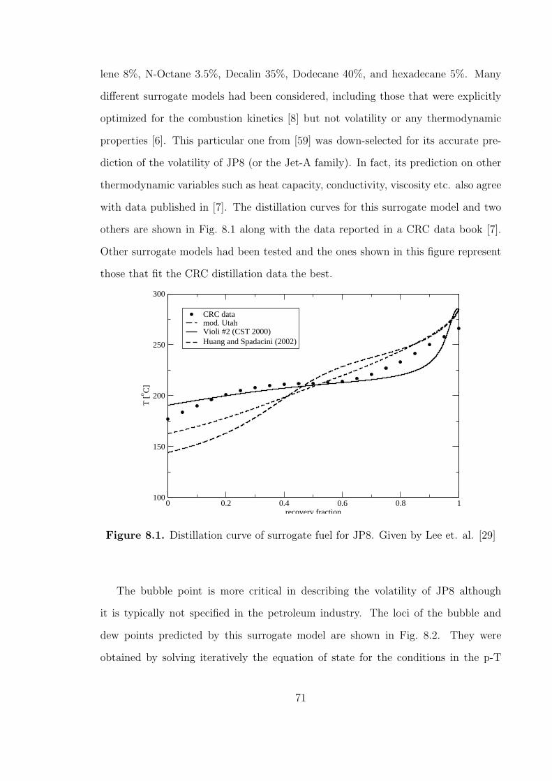
lene 8%, N-Octane 3.5%, Decalin 35%, Dodecane 40%, and hexadecane 5%. Many
different surrogate models had been considered, including those that were explicitly
optimized for the combustion kinetics [8] but not volatility or any thermodynamic
properties [6]. This particular one from [59] was down-selected for its accurate pre-
diction of the volatility of JP8 (or the Jet-A family). In fact, its prediction on other
thermodynamic variables such as heat capacity, conductivity, viscosity etc. also agree
with data published in [7]. The distillation curves for this surrogate model and two
others are shown in Fig. 8.1 along with the data reported in a CRC data book [7].
Other surrogate models had been tested and the ones shown in this figure represent
those that fit the CRC distillation data the best.
0 0.2 0.4 0.6 0.8 1recovery fraction
100
150
200
250
300
T [
o C]
CRC datamod. UtahVioli #2 (CST 2000)Huang and Spadacini (2002)
Figure 8.1. Distillation curve of surrogate fuel for JP8. Given by Lee et. al. [29]
The bubble point is more critical in describing the volatility of JP8 although
it is typically not specified in the petroleum industry. The loci of the bubble and
dew points predicted by this surrogate model are shown in Fig. 8.2. They were
obtained by solving iteratively the equation of state for the conditions in the p-T
71
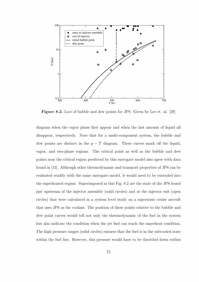
300 400 500 600 700T [K]
0.1
1
10
100
P [b
ar]
entry to injector assemblyexit of injectorinitial bubble pointdew point
Figure 8.2. Loci of bubble and dew points for JP8. Given by Lee et. al. [29]
diagram when the vapor phase first appear and when the last amount of liquid all
disappear, respectively. Note that for a multi-component system, the bubble and
dew points are distinct in the p − T diagram. These curves mark off the liquid,
vapor, and two-phase regions. The critical point as well as the bubble and dew
points near the critical region predicted by this surrogate model also agree with data
found in [13]. Although other thermodynamic and transport properties of JP8 can be
evaluated readily with the same surrogate model, it would need to be extended into
the superheated regime. Superimposed in this Fig. 8.2 are the state of the JP8 found
just upstream of the injector assembly (solid circles) and at the injector exit (open
circles) that were calculated in a system level study on a supersonic cruise aircraft
that uses JP8 as the coolant. The position of these points relative to the bubble and
dew point curves would tell not only the thermodynamic of the fuel in the system
but also indicate the condition when the jet fuel can reach the superheat condition.
The high pressure ranges (solid circles) ensures that the fuel is in the subcooled state
within the fuel line. However, this pressure would have to be throttled down within
72

the injector assembly and eventually, the fuel would exit the injector and “sees” the
combustor pressure (open circles). One can readily see that some of the open circles
lie in the two-phase and in the vapor regions. If during this transit within the injector
assembly, the flow time is shorter than the vaporization time, then, the jet fuel may
reach the superheated state.
The system level analysis provided the fuel flow rate information and thus the
characteristic flow time of the injector assembly. A comparison with the character-
istic time for the relaxation of the superheated jet fuel indicated that the two are
comparable. Thus the relaxation of the superheated fuel would have to be modeled
as a finite rate process and the Homogeneous Relaxation Model (HRM) was utilized
to describe it.
Since properties in the superheated regime cannot be measured directly (being an
unstable state), an extrapolation method was employed to calculate their values. For
a given set of variables < p, h, x > that defines a state (superheated or otherwise),
if the value of instantaneous mass fraction, x corresponds to the equilibrium value
xeq for the given < p, h > i.e. x = xeq(p, h), then the system is in the equilibrium
state. In this case, the liquid and vapor properties can be readily calculated for the
given surrogate model by the standard properties code such as SUPERTRAPP [20].
If x < xeq(p, h) then the fluid is superheated, and the liquid properties at p were
calculated by extrapolating their values from the closest regions in the pressure space
where the liquid is in the subcooled state. Note that this extrapolation scheme must
conserve the enthalpy of the two-phase fluid. To do so, first the reference pressure
p′ > p is found such that x = xeq(p′, h). This pressure p′ takes on the role of the
saturation pressure for single component systems. The liquid and vapor components
at this pressure p′ are imagined to be isolated with their respective enthalpy and
composition held fixed. Then the properties of this liquid are evaluated at several
values of pressure ≥ p′ in the subcooled state. This allowed the calculation of the
73

coefficients in a Taylor’s expansion which was used in an extrapolation step from p′
to p to get the liquid state properties at p. The properties of the vapor, on the other
hand, pose no problem as they all can be evaluated readily at p since p < p′ and
vapor would remain in the vapor state. The fluid properties for the two-phase system
are evaluated by combining the liquid and the vapor values as follows:
φ = (ν ∗ φn + (1 − ν) ∗ φn)n, n = ±1 (8.1)
Equation 8.1 represent the weighted and the weighted harmonic means. Here, φ
denotes any fluid property averaged over the two phases such as density ρ, conductiv-
ity λ, and viscosity µ; and ν denotes the weighting factor which is either the quality x
or the void fraction α. For viscosity, (8.1) was used with ν = α and n = 1. Similarly,
for thermal conductivity and density (8.1) was used with ν = x and n = 1. The mul-
ticomponent JP8 property evaluation is highly accurate in metastable region of the
two−phase system. For the single component simulations described in the previous
chapter, the REFPROP [32] suite from NIST is employed for property evaluation.
The property evaluation in the metastable region using REFPROP follows a simpler
approach where physical properties are based on their equilibrium values. Though
not exactly accurate, this is deviance in viscosity and thermal conductivity does not
cause any significant error due to the high Reynolds number of these flows.
8.2 Nozzle Results
First consider two cases both with upstream pressure fixed at 15 [bar] and the
back pressure set to 9 and 4 [bar], respectively. Fig.8.3 depicts the isocontours of
the density and the void fraction for these two cases. In both cases, vapor formation
originated at the inlet corner and developed along the length of the nozzle resulting
in the configuration of a high density core surrounded by a low density region near
the wall. The initiation of vaporization at the sharp corner is due to the sensitivity
74

of the nucleation rate to pressure and the sensitivity of the bubble growth rate to the
nucleation number density. Overall evaporation rate increases rapidly in a non-linear
fashion with the concentration of vapor bubbles because their existence dramatically
lower the energy the superheated liquid needs to overcome in order to vaporize [4].
This phenomenon is captured in the HRM model incorporated. Although the density
variation in the radial direction was significant, the fluid remained in the superheated
state throughout as the quality of the jet fuel remained low within the nozzle (a small
change in x resulted in a large change in density due to the large difference in densities
of the two phases). At the exit of the nozzle, the fluid was still in the superheated
condition. This would have significant impact on breakup of the jet core downstream
of the nozzle.
It is also evident in Fig. 8.3 that when the back pressure dropped, vaporization
became more prominent. Fig.8.6 shows the radial variation of void fraction at the exit
plane at different back pressures. The ejection angle of the fluid was also observed
to increase with decreasing back pressure which is a consequence of the increase
in vaporization. A continuous drop of back pressure however, did not result in a
corresponding linear increase in the mass flow rate. As vaporization occurs along the
nozzle, the local pressure is pushed up towards p′ (analogous to saturation pressure
for a single component system) thus attenuating the effect of a lower back pressure
in raising the mass flow rate. In the limiting case, this would result in a choking
behavior. Fig.8.4 depicts plots of the pressure along the centerline of the nozzle as
the back pressure is dropped which illustrate this phenomenon.
To further investigate the effects of choking and its mitigation strategy, simulations
were performed with the inflow pressure kept constant at 15 [bar] and dropped the
exit pressure from 14.5 [bar] to 1 [bar]. The plot depicted in Fig. 8.5 demonstrated
the phenomenon of choking as the mass flow rate plateaued at 9 [bar]. Choking
differs from the unity Mach number critical flow phenomenon in that it is due to
75
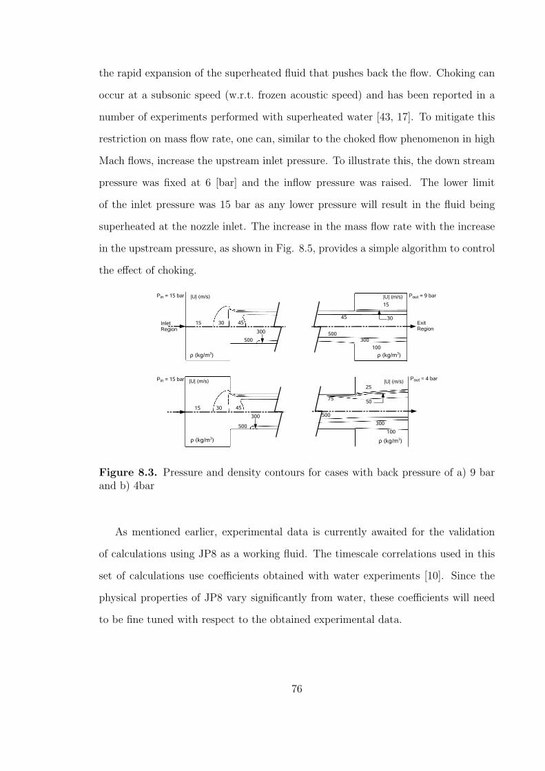
the rapid expansion of the superheated fluid that pushes back the flow. Choking can
occur at a subsonic speed (w.r.t. frozen acoustic speed) and has been reported in a
number of experiments performed with superheated water [43, 17]. To mitigate this
restriction on mass flow rate, one can, similar to the choked flow phenomenon in high
Mach flows, increase the upstream inlet pressure. To illustrate this, the down stream
pressure was fixed at 6 [bar] and the inflow pressure was raised. The lower limit
of the inlet pressure was 15 bar as any lower pressure will result in the fluid being
superheated at the nozzle inlet. The increase in the mass flow rate with the increase
in the upstream pressure, as shown in Fig. 8.5, provides a simple algorithm to control
the effect of choking.
Figure 8.3. Pressure and density contours for cases with back pressure of a) 9 barand b) 4bar
As mentioned earlier, experimental data is currently awaited for the validation
of calculations using JP8 as a working fluid. The timescale correlations used in this
set of calculations use coefficients obtained with water experiments [10]. Since the
physical properties of JP8 vary significantly from water, these coefficients will need
to be fine tuned with respect to the obtained experimental data.
76
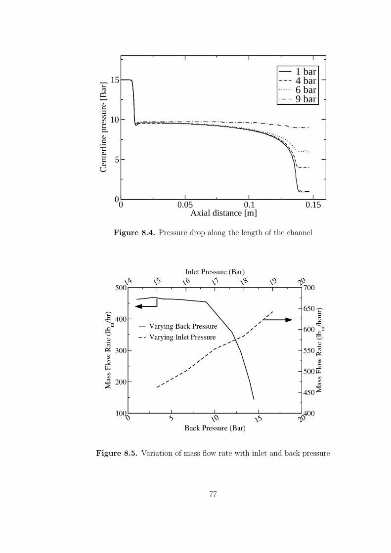
0 0.05 0.1 0.15Axial distance [m]
0
5
10
15
Cen
terl
ine
pres
sure
[B
ar]
1 bar4 bar6 bar9 bar
Figure 8.4. Pressure drop along the length of the channel
Figure 8.5. Variation of mass flow rate with inlet and back pressure
77
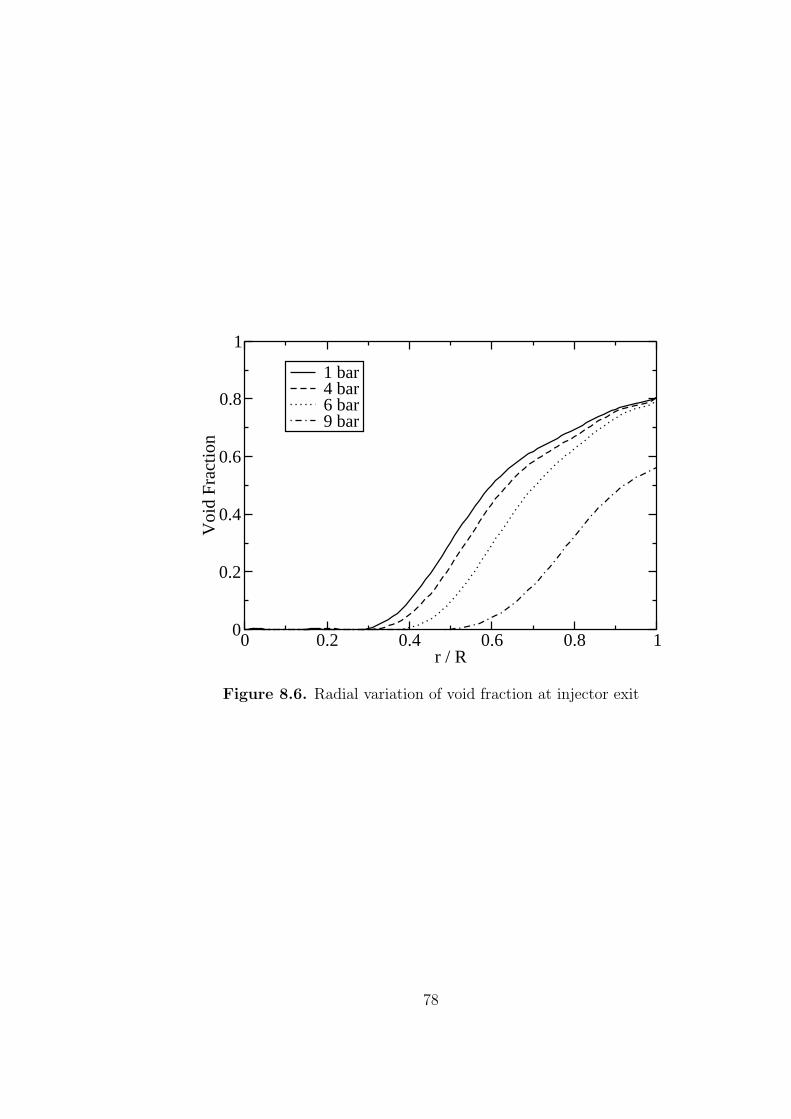
0 0.2 0.4 0.6 0.8 1r / R
0
0.2
0.4
0.6
0.8
1
Voi
d Fr
actio
n
1 bar4 bar6 bar9 bar
Figure 8.6. Radial variation of void fraction at injector exit
78
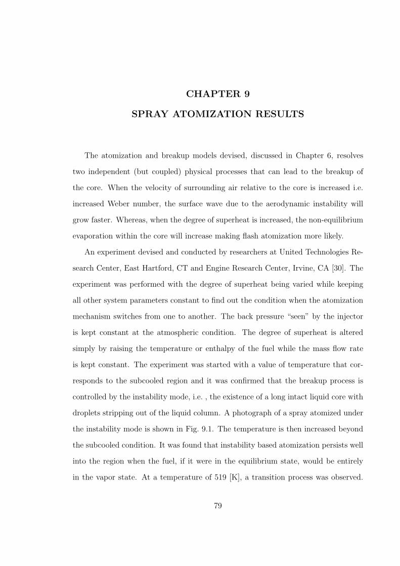
CHAPTER 9
SPRAY ATOMIZATION RESULTS
The atomization and breakup models devised, discussed in Chapter 6, resolves
two independent (but coupled) physical processes that can lead to the breakup of
the core. When the velocity of surrounding air relative to the core is increased i.e.
increased Weber number, the surface wave due to the aerodynamic instability will
grow faster. Whereas, when the degree of superheat is increased, the non-equilibrium
evaporation within the core will increase making flash atomization more likely.
An experiment devised and conducted by researchers at United Technologies Re-
search Center, East Hartford, CT and Engine Research Center, Irvine, CA [30]. The
experiment was performed with the degree of superheat being varied while keeping
all other system parameters constant to find out the condition when the atomization
mechanism switches from one to another. The back pressure “seen” by the injector
is kept constant at the atmospheric condition. The degree of superheat is altered
simply by raising the temperature or enthalpy of the fuel while the mass flow rate
is kept constant. The experiment was started with a value of temperature that cor-
responds to the subcooled region and it was confirmed that the breakup process is
controlled by the instability mode, i.e. , the existence of a long intact liquid core with
droplets stripping out of the liquid column. A photograph of a spray atomized under
the instability mode is shown in Fig. 9.1. The temperature is then increased beyond
the subcooled condition. It was found that instability based atomization persists well
into the region when the fuel, if it were in the equilibrium state, would be entirely
in the vapor state. At a temperature of 519 [K], a transition process was observed.
79
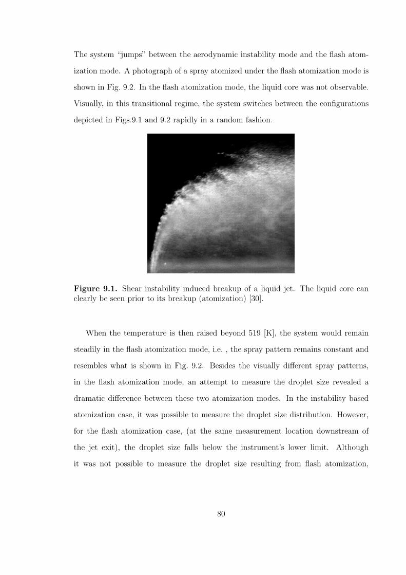
The system “jumps” between the aerodynamic instability mode and the flash atom-
ization mode. A photograph of a spray atomized under the flash atomization mode is
shown in Fig. 9.2. In the flash atomization mode, the liquid core was not observable.
Visually, in this transitional regime, the system switches between the configurations
depicted in Figs.9.1 and 9.2 rapidly in a random fashion.
Figure 9.1. Shear instability induced breakup of a liquid jet. The liquid core canclearly be seen prior to its breakup (atomization) [30].
When the temperature is then raised beyond 519 [K], the system would remain
steadily in the flash atomization mode, i.e. , the spray pattern remains constant and
resembles what is shown in Fig. 9.2. Besides the visually different spray patterns,
in the flash atomization mode, an attempt to measure the droplet size revealed a
dramatic difference between these two atomization modes. In the instability based
atomization case, it was possible to measure the droplet size distribution. However,
for the flash atomization case, (at the same measurement location downstream of
the jet exit), the droplet size falls below the instrument’s lower limit. Although
it was not possible to measure the droplet size resulting from flash atomization,
80

Figure 9.2. Flash vaporization induced breakup of a superheated jet. The liquidcore disappeared and the atomization process occurs near the exit of the nozzle orifice.[30]
visual confirmation was achieved that there were fine droplets resulting from the
flash atomization process.
The atomization model can be exercised at any point in the subcritical region of
the P-T space (excluding the solid regime). The models then can be utilized to find
out in the P-T space, the regions where atomization is effected either by the shear or
the flashing mode. A binary cut algorithm was coupled to the atomization model in
the following way. For each value of P , a search is initialized by setting two values
of T i.e. Tmin and Tmax such that the primary breakup is caused by shear instability
at T = Tmin and by flashing at T = Tmax. These two values always exist since one
can put simply Tmin = Tbub − 1 and Tmax = Tsuperheat limit + 1. This is followed by
the standard binary cut algorithm to locate the transition value of T for the given
value of P i.e. T = T (P ) such that when T < T , instability based atomization occurs;
when T > T , flash atomization takes place. The locus of T (P ) is dependent on the
air velocity relative to the liquid core at the exit of the nozzle. High values of this
relative velocity favors the shear instability breakup mode.
81
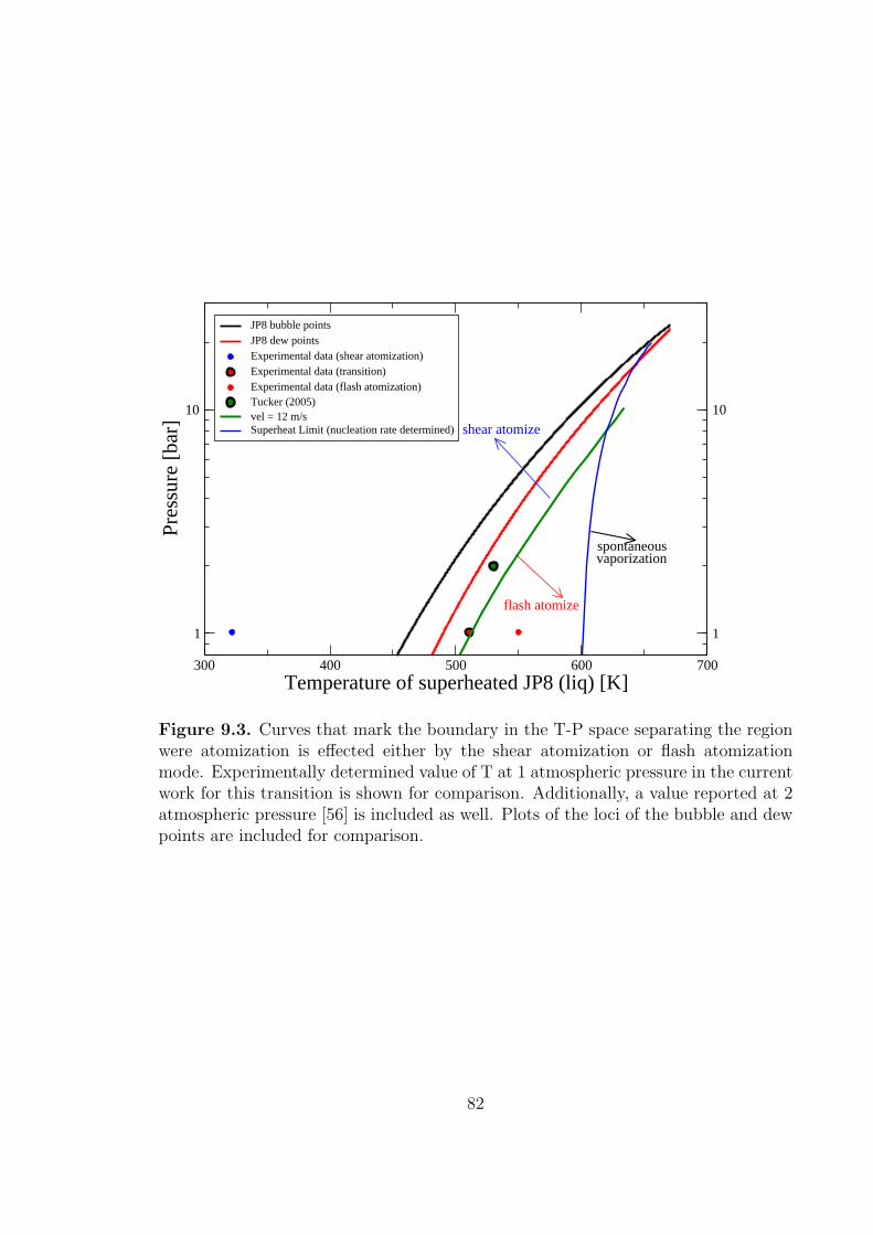
300 400 500 600 700Temperature of superheated JP8 (liq) [K]
1 1
10 10
Pres
sure
[ba
r]
JP8 bubble pointsJP8 dew pointsExperimental data (shear atomization)Experimental data (transition)Experimental data (flash atomization)Tucker (2005)vel = 12 m/sSuperheat Limit (nucleation rate determined)
flash atomize
shear atomize
spontaneousvaporization
Figure 9.3. Curves that mark the boundary in the T-P space separating the regionwere atomization is effected either by the shear atomization or flash atomizationmode. Experimentally determined value of T at 1 atmospheric pressure in the currentwork for this transition is shown for comparison. Additionally, a value reported at 2atmospheric pressure [56] is included as well. Plots of the loci of the bubble and dewpoints are included for comparison.
82

The loci of the transitional points T (P ) are plotted as the green curve in Fig.
9.3 using the value of the relative air velocity employed in the experiment. The
corresponding transitional point at P = 1.01325 [bar] measured experimentally is
depicted as the black circle with a red core in Fig. 9.3. One can see that the theoretical
prediction agrees with the experimental datum. In Tucker et al. [56], a transitional
point at 2 atmospheric pressure was estimated theoretically and later on verified
experimentally. This point is also reported in Fig. 9.3 as the black circle with a green
core at 2.265 [bar].
The green curve in Fig. 9.3 shows the transition temperature for different values
of pressure. As can be expected, higher values of pressure requires a higher degree
of superheat to induce flash atomization. A designer can simply use the green curve
to figure out the temperature required, for given values of pressure and jet relative
velocity, to take advantage of flash atomization. Although not shown, when the
relative jet velocity is increased, the green curve moves to the right. This is so
because an increase in the relative jet velocity would raise the Weber number which in
turns would make the shear layer more unstable. Consequently, the flash atomization
would have to occur at a higher degree of superheat. The nucleation rate imposed
superheat limit is also depicted in Fig. 9.3. This curve intersects the shear-flash
atomization transition curve. Thus, for a given value of the relative jet velocity and at
a sufficiently high ambient pressure, as one increases the fluid temperature, one would
cross the superheat limit curve first. In this case, as the temperature is increased,
the superheated fluid will never undergo the finite rate vaporization (controlled by
nucleation and bubble growth), but instead, will undergo spontaneous vaporization
when this limit curve is crossed - the atomization step is bypassed entirely. Thus, Fig.
9.3 describes all the vaporization modes exhibited by a supheated jet: atomization
due to shear instability, atomization due to the finite rate relaxation of a superheated
fluid, and the spontaneous vaporization of the fluid.
83
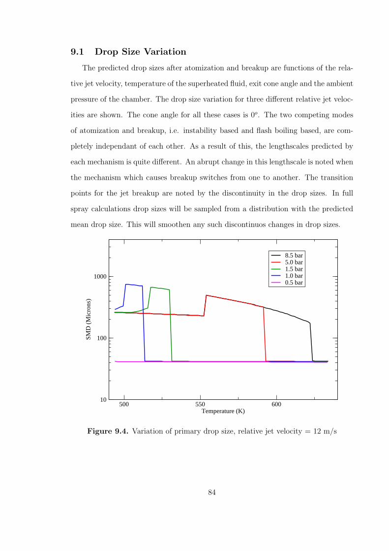
9.1 Drop Size Variation
The predicted drop sizes after atomization and breakup are functions of the rela-
tive jet velocity, temperature of the superheated fluid, exit cone angle and the ambient
pressure of the chamber. The drop size variation for three different relative jet veloc-
ities are shown. The cone angle for all these cases is 0o. The two competing modes
of atomization and breakup, i.e. instability based and flash boiling based, are com-
pletely independant of each other. As a result of this, the lengthscales predicted by
each mechanism is quite different. An abrupt change in this lengthscale is noted when
the mechanism which causes breakup switches from one to another. The transition
points for the jet breakup are noted by the discontinuity in the drop sizes. In full
spray calculations drop sizes will be sampled from a distribution with the predicted
mean drop size. This will smoothen any such discontinuos changes in drop sizes.
500 550 600Temperature (K)
10
100
1000
SMD
(M
icro
ns)
8.5 bar5.0 bar1.5 bar1.0 bar0.5 bar
Figure 9.4. Variation of primary drop size, relative jet velocity = 12 m/s
84
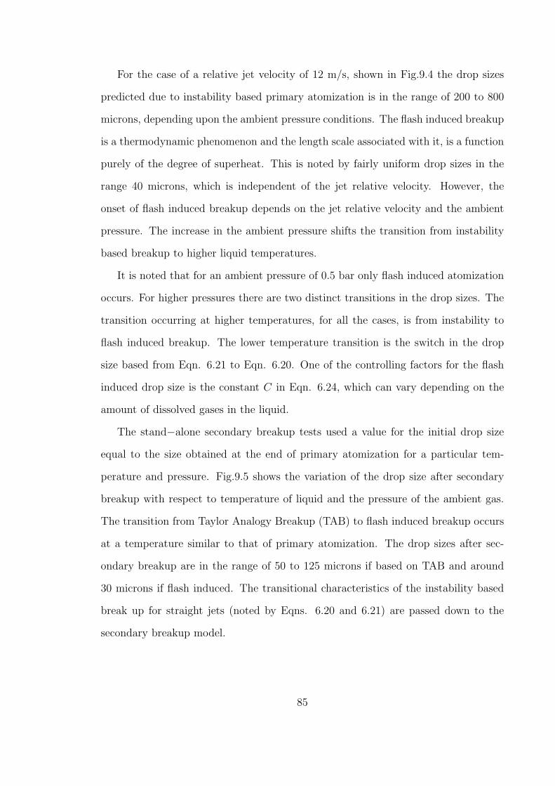
For the case of a relative jet velocity of 12 m/s, shown in Fig.9.4 the drop sizes
predicted due to instability based primary atomization is in the range of 200 to 800
microns, depending upon the ambient pressure conditions. The flash induced breakup
is a thermodynamic phenomenon and the length scale associated with it, is a function
purely of the degree of superheat. This is noted by fairly uniform drop sizes in the
range 40 microns, which is independent of the jet relative velocity. However, the
onset of flash induced breakup depends on the jet relative velocity and the ambient
pressure. The increase in the ambient pressure shifts the transition from instability
based breakup to higher liquid temperatures.
It is noted that for an ambient pressure of 0.5 bar only flash induced atomization
occurs. For higher pressures there are two distinct transitions in the drop sizes. The
transition occurring at higher temperatures, for all the cases, is from instability to
flash induced breakup. The lower temperature transition is the switch in the drop
size based from Eqn. 6.21 to Eqn. 6.20. One of the controlling factors for the flash
induced drop size is the constant C in Eqn. 6.24, which can vary depending on the
amount of dissolved gases in the liquid.
The stand−alone secondary breakup tests used a value for the initial drop size
equal to the size obtained at the end of primary atomization for a particular tem-
perature and pressure. Fig.9.5 shows the variation of the drop size after secondary
breakup with respect to temperature of liquid and the pressure of the ambient gas.
The transition from Taylor Analogy Breakup (TAB) to flash induced breakup occurs
at a temperature similar to that of primary atomization. The drop sizes after sec-
ondary breakup are in the range of 50 to 125 microns if based on TAB and around
30 microns if flash induced. The transitional characteristics of the instability based
break up for straight jets (noted by Eqns. 6.20 and 6.21) are passed down to the
secondary breakup model.
85
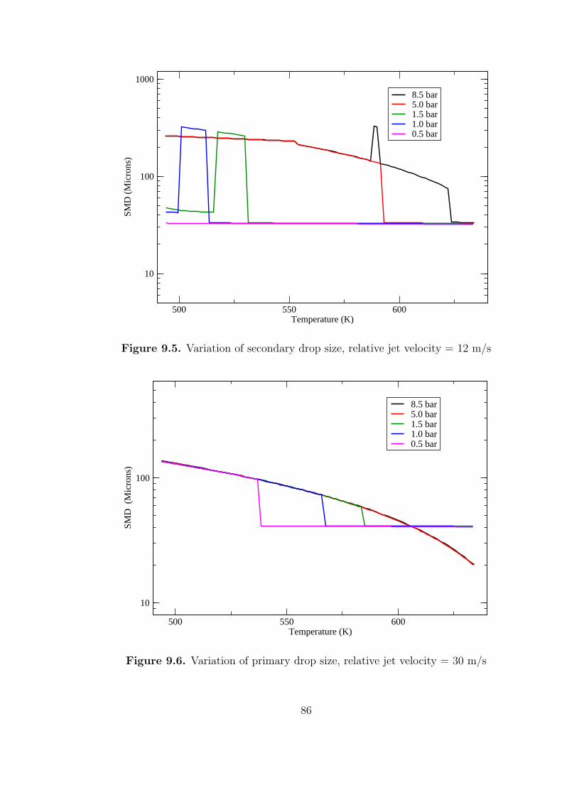
500 550 600Temperature (K)
10
100
1000
SMD
(M
icro
ns)
8.5 bar5.0 bar1.5 bar1.0 bar0.5 bar
Figure 9.5. Variation of secondary drop size, relative jet velocity = 12 m/s
500 550 600Temperature (K)
10
100
SMD
(M
icro
ns)
8.5 bar5.0 bar1.5 bar1.0 bar0.5 bar
Figure 9.6. Variation of primary drop size, relative jet velocity = 30 m/s
86

500 550 600Temperature (K)
1
10
100SM
D (
Mic
rons
)
8.5 bar5.0 bar1.5 bar1.0 bar0.5 bar
Figure 9.7. Variation of secondary drop size, relative jet velocity = 30 m/s
At higher relative jet velocities, a strong prominence of instability based atomiza-
tion and breakup is expected and observed in the calculations. For sufficiently high
pressures such as 5 bar and 8.5 bar, the transition to flash induced breakup does not
take place in the investigated temperature range. The drop sizes obtained at higher
relative jet velocities are significantly smaller as well as shown in Figs.9.6,9.7,9.8 and
9.9. For the instability based primary atomization, the breakup characteristic of the
straight jet always follows Eqn. 6.20. Hence for each case there is only one transition
point for primary atomization.
87
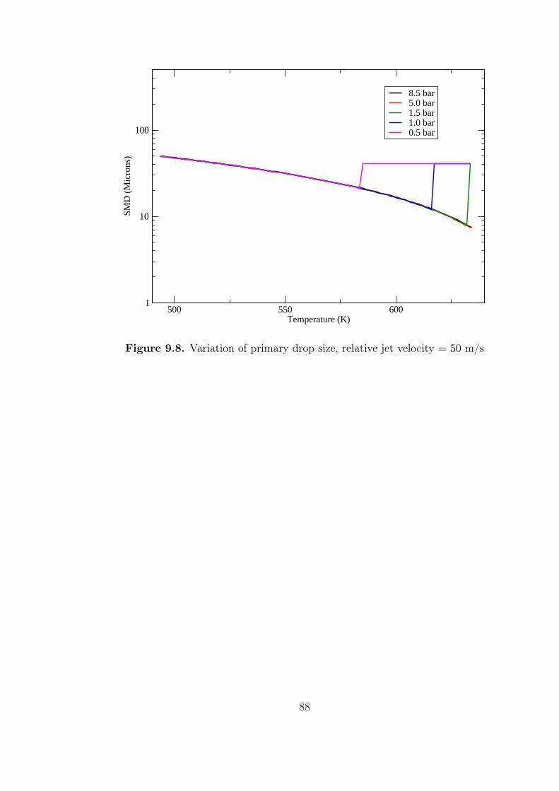
500 550 600Temperature (K)
1
10
100SM
D (
Mic
rons
)
8.5 bar5.0 bar1.5 bar1.0 bar0.5 bar
Figure 9.8. Variation of primary drop size, relative jet velocity = 50 m/s
88
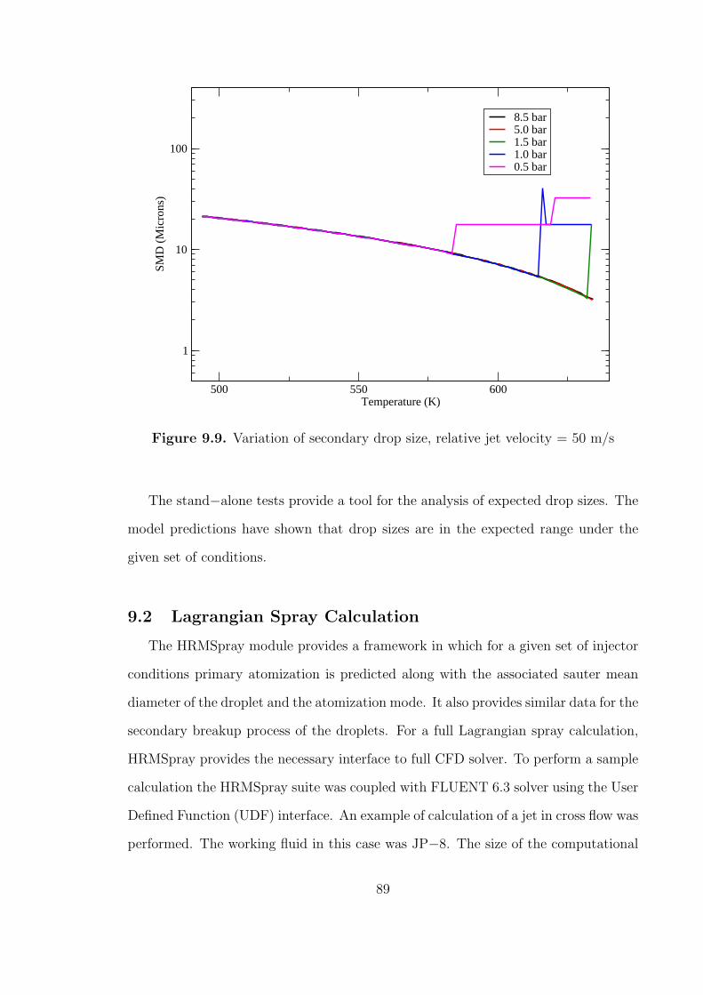
500 550 600Temperature (K)
1
10
100SM
D (
Mic
rons
)
8.5 bar5.0 bar1.5 bar1.0 bar0.5 bar
Figure 9.9. Variation of secondary drop size, relative jet velocity = 50 m/s
The stand−alone tests provide a tool for the analysis of expected drop sizes. The
model predictions have shown that drop sizes are in the expected range under the
given set of conditions.
9.2 Lagrangian Spray Calculation
The HRMSpray module provides a framework in which for a given set of injector
conditions primary atomization is predicted along with the associated sauter mean
diameter of the droplet and the atomization mode. It also provides similar data for the
secondary breakup process of the droplets. For a full Lagrangian spray calculation,
HRMSpray provides the necessary interface to full CFD solver. To perform a sample
calculation the HRMSpray suite was coupled with FLUENT 6.3 solver using the User
Defined Function (UDF) interface. An example of calculation of a jet in cross flow was
performed. The working fluid in this case was JP−8. The size of the computational
89

domain was set 0.05mx0.05mx0.1m. The injector was located at the coordinate [-
0.02499 0.0 0.025]. A steady state solver has been used to resolve the flow in the gas
phase. A finite number of unsteady Lagrangian particles were injected in the time it
took the steady state solver to reach convergence.
The particle tracking was set to be unsteady, with 500 particles being injected
every time step, which was set to 5e-6 s. The injector diameter was 0.508 mm and
the injection velocity was 40.85 m/s. The liquid temperature for this case was 540 K.
The exit cone angle for the jet was 30o and the critical void fraction at which breakup
occurs for flash based atomization was assumed to be 0.6.
A cross flow velocity of 120 m/s was set in the z−direction. The boundary layer
thickness was assumed to be 10mm based on discussions with Energy Research Con-
sultants. This sample calculation was used to illustrate the usage of the atomization
model to predict the breakup length and the path of the droplet. The vaporization
model for the particle injections was not used in this calculation as mass transport
equation was not solved in this demonstration.
Figs.9.10 and 9.11 show the velocity and pressure contours at a plane [y=0]. The
velocity plot clearly shows the developed boundary layer and the effect of the jet.
The particle tracks shown in Fig.9.12, which is a close−up image, reveals the
divergence of the jet as it exits the nozzle. The cross flow velocity causes a strong
asymmetry, blowing the jet downstream in the direction of the cross flow velocity.
As the jet exits the boundary layer and reaches the zone of the free stream gas
phase velocity the effect of being pushed downstream becomes more pronounced.
The predicted sauter mean diameter for the entire spray is calculated as 33 microns.
90

Contours of Velocity Magnitude (m/s)FLUENT 6.3 (3d, dp, pbns, ske)
Dec 08, 2009
1.20e+021.14e+021.08e+021.02e+029.64e+019.03e+018.43e+017.83e+017.23e+016.62e+016.02e+015.42e+014.82e+014.22e+013.61e+013.01e+012.41e+011.81e+011.20e+016.02e+000.00e+00
Z
Y
X
Figure 9.10. Velocity contours, Boundary layer = 10 mm
91
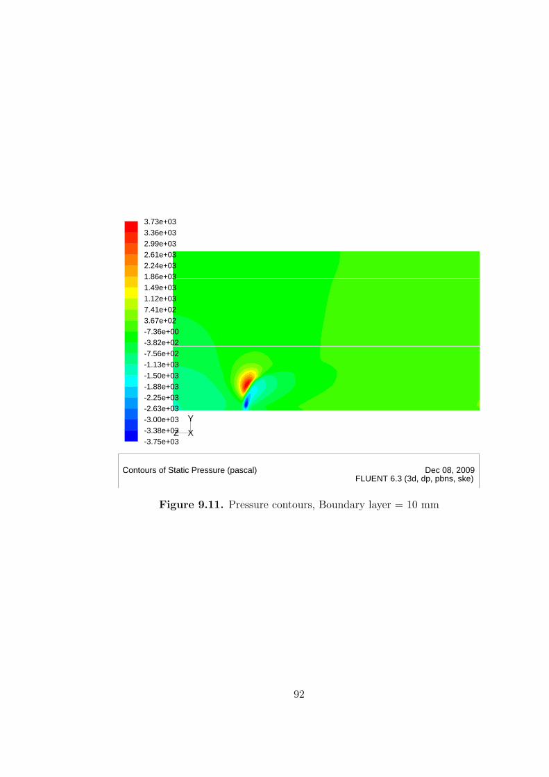
Contours of Static Pressure (pascal)FLUENT 6.3 (3d, dp, pbns, ske)
Dec 08, 2009
3.73e+033.36e+032.99e+032.61e+032.24e+031.86e+031.49e+031.12e+037.41e+023.67e+02-7.36e+00-3.82e+02-7.56e+02-1.13e+03-1.50e+03-1.88e+03-2.25e+03-2.63e+03-3.00e+03-3.38e+03-3.75e+03
Z
Y
X
Figure 9.11. Pressure contours, Boundary layer = 10 mm
92
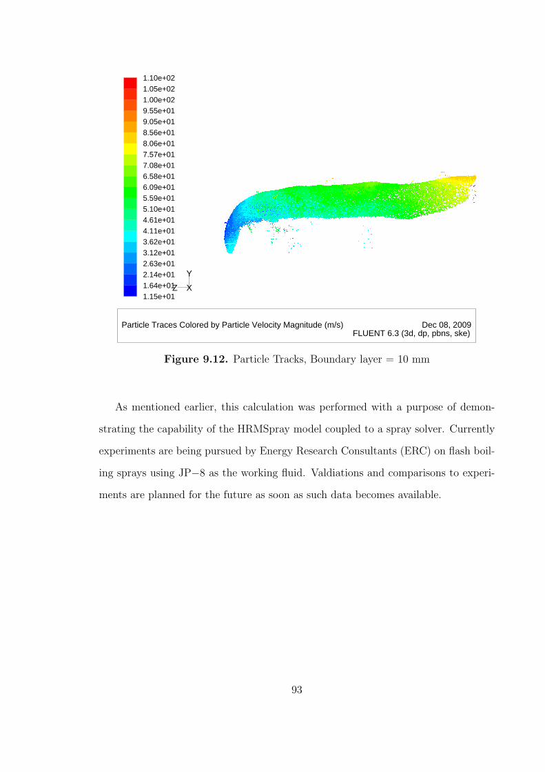
Particle Traces Colored by Particle Velocity Magnitude (m/s)FLUENT 6.3 (3d, dp, pbns, ske)
Dec 08, 2009
1.10e+021.05e+021.00e+029.55e+019.05e+018.56e+018.06e+017.57e+017.08e+016.58e+016.09e+015.59e+015.10e+014.61e+014.11e+013.62e+013.12e+012.63e+012.14e+011.64e+011.15e+01
Z
Y
X
Figure 9.12. Particle Tracks, Boundary layer = 10 mm
As mentioned earlier, this calculation was performed with a purpose of demon-
strating the capability of the HRMSpray model coupled to a spray solver. Currently
experiments are being pursued by Energy Research Consultants (ERC) on flash boil-
ing sprays using JP−8 as the working fluid. Valdiations and comparisons to experi-
ments are planned for the future as soon as such data becomes available.
93
CHAPTER 10
SUMMARY
At elevated temperatures the interphase heat transfer is the main mechanism
which provides enthalpy for phase change. This causes the fluid to be in thermody-
namic nonequilibrium when the flow–through time is comparable to the relaxation
time. The thermal nonequilibrium has been modeled and tested as a finite rate heat
process. The Homogenous Relaxation Model (HRM) has been successfully demon-
strated as a model for the phase change process in flash–boiling flows.
A new solver for internal nozzle flows was constructed using OpenFOAM, an
object-oriented framework that supports a variety of discretization schemes and poly-
hedral meshes and is parallelized using MPI. The model was validated with several
experiments from literature. Phenomena such as “vapor lock” and “two-phase sub-
sonic choking” observed in experiments were reproduced numerically in simulations.
External spray atomization and breakup models were constructed in conjuction
with phase change model. These models provide dual mode breakup mechanisms
which rely on aerodynamic instabilities and internal phase change processes. An
identification of regimes in thermodynamic state space was carried out to reveal the
dominant process of droplet formation.
10.1 Future Work
10.1.1 Fuel properties
The fuel property database is currently can provide data for single component
fluids and one multicomponent fuel, namely JP8 (jet fuel). Extensions to fuel prop-
94
erty database to incorporate several multicomponent fuels such as gasoline, gasoline–
ethanol blends etc., are at present underway. This will enable further investigations of
realistic fuel properties, including the effects of transport properties such as viscosity.
10.1.2 Validation and Adjustments of Coefficients
The lack of experimental data for validation is a concern; experimental data for
internal flows using realistic fuels are not available at present. It is anticipated that,
due to the importance of flash-boiling, more experimental investigations of internal
nozzle flow with fuels will soon be published. At that time, further validation of this
model will be possible.
The finite rate phase change model is based on an empirical timescale relationship.
The coefficients for this equation are based on experimental data obtained for water.
Though these provide a good starting point for calculations using hydrocarbons as
working fluids, it is expected that these will need to be fine tuned once experimental
data using such fluids becomes available.
10.1.3 Nucleation Model
Dissolved gases and impurities in the working fluid start as nucleations sites for
phase change process. The number of these germination sites can vary with the qual-
ity of the fluid used and physical parameters such as pressure and temperature. A
rudimentary constant nucleation model was implemented in this study which uses a
fixed value. A sophisticated nucleation model which considers thermophysical vari-
ables is expected to improve the fidelity of the CFD calculations.
95

BIBLIOGRAPHY
[1] Aquino, C., Plensdorf, W., Lavoie, G., and Curtis, E. The occurence of FlashBoiling in Port Injected Gasoline Engines. SAE Paper 982522 (1998).
[2] Barret, Michel, Faucher, Eric, and Herard, Jean-Marc. Schemes to computeunsteady flashing flows. AIAA Journal 40, 5 (2002).
[3] Bilicki, Z., and Kestin, J. Physical aspects of the relaxation model in two-phaseflow. Proc. Roy. Soc. London A. 428 (1990), 379–397.
[4] Blander, M., and Katz, J. L. Bubble nucleation in liquids. ALCHE J. 21 (1975),833–848.
[5] Conway, John Horton, and Sloane, Neil J. A. Sphere Packings, Lattices andGroups (Grundlehren Der Mathematischen Wissenschaften) ISBN: 0387979123,2nd ed. Spinger, Nov 1992.
[6] Cooke, J. A., Bellucci, M., Smooke, M. D., Gomez, A., Violi, A., Faravelli, T.,and Ranzi, E. Computational and experimental study of jp-8, a surrogate, andits components in counterflow diffusion flames. Proc. Comb. Inst. 30 (2005),439–446.
[7] Coordinating Research Council Inc. Ed. Handbok of Aviation Fuel Properties,Third Edition CRC report No. 530. 1983, 2004.
[8] Dagaut, P., and Cathonnet, M. The ignition, oxidation, and combustion ofkerosene: A review of experimental and kinetic modeling. Prog. in Energy andCombustion Science 32 (2006), 48–92.
[9] Dombrowski, N., and Hooper, P.C. The effect of ambient density on drop for-mation in sprays. Chem. Eng. Sci. 17 (1962), 291–305.
[10] Downar-Zapolski, P., Bilicki, Z., Bolle, L., and Franco, J. The Non-equilibriumRelaxation Mokdel for One-Dimensional Flashing Liquid Flow. Int. J. MultiphasePhase Flow 22-3 (1996), 473–483.
[11] Downar-Zapolski, P., Bilicki, Z., Bolle, L., and Franco, J. The Non-EquilibriumRelaxation Model for One-Dimensional Flashing Liquid Flow. IJMF 22, 3 (1996),473–483.
[12] Duan, Ri-Qiang, Jiang, Sheng-Yao, Koshizuka, Seiichi, Oka, Yoshiaki, and Ya-maguchi, Akira. Direct simulation of flashing liquid jets using the mps method.Intl. J. of Heat and Mass Trans. 49 (2006), 402–405.
96
[13] Edwards, Tim, and Maurice, Lourdes Q. Surrogate Mixtures to Represent Com-plex Aviation and Rocket Fuels. J. Prop. Power 17-2 (2001), 461–466.
[14] Einstein, A. Uber Schallschwingungen in teilweise dissocierten Gasen. SitzungBerl. Akad. Physik Chemie (1920), 380–385.
[15] et al., E. Sher. Flash-boiling atomization. Progress Energy Combust Sci. in press(2007).
[16] et al., J.A. Boure. Highlights of two-phase flow: on the links between maximumflow rates, sonic velocities, propogation and transfer phenomena in single andtwo-phase flows. Int. J. Multiphase Flow 3 (1976), 1–22.
[17] Fauske, H. K. The discharge of saturated water through tubes. Chem. Eng.Prog. Symp. Ser. 6 (1965), 210–216.
[18] Ferziger, Joel H., and Peric, Milovan. Computational Methods for Fluid Dynam-ics, 3rd ed. Springer, 2002.
[19] Henry, R.E., and Fauske, H.K. The two-phase critical flow of one-componentmixtures in nozzles, orifices, and short tubes. Heat Transfer 93, 2 (1971), 179–187.
[20] Huber, M. L. SUPERTRAPP: Thermophysical properties of Hydrocarbon Mix-tures Database. U.S. Department of Commerce, NIST, Gaithersburg MD 20899(Feb. 2003).
[21] Issa, R. I. Solution of the implicitly discretised fluid flow equations by operator-splitting. J. Comput. Phys. 62, 1 (1986), 40–65.
[22] Jasak, H. Error Analysis and Estimation for the Finite Volume Method withApplications to Fluid Flows. PhD thesis, Imperial College, 1996.
[23] Karypis, George, and Kumar, Vipin. MeTis: Unstrctured Graph Partitioningand Sparse Matrix Ordering System, Version 2.0, 1995.
[24] Kato, H., Kayano, H., and Kageyama, Y. A Consideration of Thermal Effects onCavitation Bubble Growth. In Cavitation and Multiphase Flow (1994), vol. 194of FED, ASME.
[25] Kawano, Daisuke, Goto, Yuichi, Odaka, Matsuo, and Senda, Jiro. Modellingatomization and vaporization processes of flash-boiling spray. SAE 2004-01-0534(2004).
[26] Kawano, Daisuke, Ishii, hajime, Suzuki, Hisakazu, Goto, Yuichi, Odaka, Matsuo,and Senda, Jiro. Numerical study on flashin-boiling spray of multicomponentfuel. Heat Transfer-Asian Research (Wiley Periodicals, Inc.) 35(5) (2006), 369–385.
97

[27] Kim, Y., and O’Neal, D. L. An experimental study of two-phase flow of hfc-134a through short tube orifices. Heat Pump and Refrigeration Systems Design,Analysis, and Applications 29 (1993), 1–8.
[28] Knapp, Robert T., Daily, James W., and Hammitt, Fredrick G. Cavitation.McGraw-Hill, 1970.
[29] Lee, J., Madabhushi, R., Fotache, C. Gopalakrishnan, S., and Schmidt, D. Flash-ing flow of superheated jet fuel. Proc. Comb. Inst. In Press, Obtainable at:http:dx.doi.org (2008), doi:10.1016j.proci.2008.06.153.
[30] Lee, J. C., M., Corn, C., Fotache, S., Gopalakrishnan, and P., Schmidt D. At-omization of superheated jet fuel. In preparation.
[31] Lee, J. C., R., Madabushi, C., Fotache, S., Gopalakrishnan, and P, Schmidt D.Flashing flow of superheated jet fuel. Proceedings of Combustion Institute 32, 2(2008), 3215 –3222.
[32] Lemmon, E.W., Huber, M.L., and McLinden, M.O. NIST Standard Refer-ence Database 23: Reference Fluid Thermodynamic and Transport Properties-REFPROP, version 8.0 standard reference data program ed. National Instituteof Standards and Technology, Gaithersburg, 2007.
[33] Minato, Akihiko, Takamori, Kazuhide, and Susuki, Akira. Numerical study oftwo-dimensional structure in critical steam-water two-phase flow. Journal ofNuclaear Science and Technology 35, 5 (May 1995), 464–475.
[34] Moody, F.J. Maximum flow rate of a single component, two-phase mixture. J.Heat Transfer 87, 1 (1965), 134–142.
[35] Nouri, J.M., Mitroglou, N., Yan, Y., and Arcoumanis, C. Internal Flow andCavitation in a Multi-Hole Injector for Gasoline Direct-Injection Engines. SAEPaper 2007-01-1405 (2007).
[36] Nurick, W.H. Orifice cavitation and its effect on spray mixing. Journal of FuidsEgineering-Transactions of the ASME 98, 4 (1976), 681–687.
[37] oes Moreira, J. R. Sim and Bullard, C. W. Pressure drop and flashing mecha-nisms in refrigerant expansion devices. Int. J. of Refrigeration 26 (2003), 840–848.
[38] OpenCFD. OpenFOAM - The Open Source CFD Toolbox - Programmers Guide,1.4.1 ed. OpenCFD Ltd., United Kingdom, 11 Apr. 2007.
[39] O’Rourke, P. J., and A., Amsden A. The tab method for numerical calculationof spray droplet breakup. SAE 872089 (Nov 1987).
[40] Oza, R.D., and Sinnamon, J.F. An Experimental and Analytical Study of Flash-Boiling Fuel Injection. SAE Paper 830590 (1983).
98

[41] Park, B.S., and Lee, S. Y. An Experimental Investigation of the Flash Atomiza-tion Mechanism. Atomization and Sprays 4 (1994), 159–179.
[42] Reitz, R. D. Modeling atomization processes in high-pressure vaporizing sprays.Atomization and Spray Technology 3 (1987), 309–337.
[43] Reitz, Rolf D. A Photographic Study of Flash-Boiling Atomization. AerosolScience and Technology 12 (1998), 561–569.
[44] Schmidt, David P. Cavitation in Diesel Fuel Injector Nozzles. PhD thesis, Uni-versity of Wisconsin Madison, December 1997.
[45] Schmidt, David P., Chiappeta, Louis M., Goldin, Graham M., and Madabbushi,Rabi K. Transient multidimensional modeling of air-blast atomizers. Atomizationand Sprays 13 (2003), 357–377.
[46] Schmidt, David P., Rutland, C. J., Corradini, M. L., Roosen, P., and Genge, O.Cavitation in asymmetric two-dimensional nozzles. Journal of Engines 108, 3(1999), 613–629.
[47] Schmidt, D.P., Corradini, M.L., and Rutland, C.J. A Two-Dimensional, Non-Equilibrium Model of Flashing Nozzle Flow. In Proc. of 3rd ASME/JSME JointFluids Engineering Conference (1999), FEDSM.
[48] Schmidt, D.P., Rutland, C.J., and Corradini, M.L. A Fully Compressible Modelof Cavitating Flow. Atomization and Sprays 9 (1999), 255–276.
[49] Schmitz, Ingo, Ipp, Wolfgang, and Leipertz, Alfred. Flash Boiling Effects on theDevelopment of Gasoline Direct - Injection Engine Sprays. SAE Paper 2002-01-2661 (2002).
[50] Schulz, W. D. Oxidation Products of s Surrogate JP-8 Fuel. Symposium onStructure of Jet Fuels III (April 5-10 1991), 383–391.
[51] Senda, J., Yoshiyuki, H., and Hajime, F. Modeling on atomization adn aporiza-tion process in flash boiling spray. JSAE Review 15 (1994), 291–296.
[52] Senecal, P. K., Schmidt, D. P., Nouar, I., Rutland, C. J., Reitz, Rl. D., andCorradini, M. L. Modeling high-speed viscous liquid sheet atomization. Int. J.Multiphase Flow 25 (1999), 1073–1097.
[53] Sher, Eran, and Chalm, Elata. Spray formation from pressure cans by flashing.Ind. Eng. Chem., Process Des. Dev. 16(2) (1977), 237–242.
[54] Spadaccini, L. J., and Huang, H. On-Line Fuel Deoxygenation for Coke Sup-pression. Transactions of the ASME 125 (2003), 686–692.
[55] Tikhonenko, L.K., Kevorkov, L.P., and Lutovinov, S.Z. An investigation of thelocal paramters of critical flow of hot water in straight pipes with a sharp inletedge. Teploenergetika 25, 2 (1978), 41–44.
99
[56] Tucker, Kelly Colin. A Flash Vaporization System for Detonation of HydrocarbonFuels in a Pulse Detonation Engine, afitdseny05-03 ed. Dept. US Air Force, AirUniversity, 2005.
[57] Valero, E., and Parra, I.E. The role of thermal diseqilibrium in critical two-phaseflow. Multiphase Flow 28 (2002), 21–50.
[58] VanDerWege, B. A. The effect of fuel volatility and operating conditions on sprayfrom pressure swirl fuel injectors. PhD thesis, M.I.T., 1999.
[59] Violi, A, Yan, S., Eddings, E. G., Sarofim, F., Franata, S., Faravelli, T., andRanzi, E. Experimental formulation adn kinetic model for jp-8 surrogate mix-tures. Combust. Science and Tech. 174(11-2) (2002), 399–417.
[60] Vortmann, C., Schnerr, G.H., and Seelecke, S. Thermodynamic modeling andsimulation of cavitating nozzle flow. Int. J. of Heat and Fluid Flow 24 (2003),774–783.
[61] Wada, Yoshimitsu, Nishimura, Yuji, Yamaguchi, Akihiro, Magara, Noriyuki,Senda, Jiro, and Fujimoto, Hajime. Controlling PCCI Combustion with MixedFuel - Application of Flashing Spray to Early Injection. SAE Paper 2007-01-0624(2007).
[62] Wallis, G.B. Critical two-phase flow. Multiphase Flow 6 (1980), 97–112.
[63] Weller, Henry G., G.Tabor, Jasak, Hrvoje, and Fureby, C. A Tensorial Ap-proach to Computational Continuum Mechanics Using Object–Oriented Tech-niques. Computers in Physics 12, 6 (1998), 620–63.
[64] Wu, P-K, Shahnam, M., Kirkendall, K., A., C., Carter, and A., Nejad. Expan-sion and Mixing Processes of Underexpanded Supercritical Fuel Jets Injectedinto Superheated Conditions 9. 33rd AIAA/ASME/SAE/ASEE Joint Propul-sion Conference and Exhibit July 6-9 Seattle, WA AIAA 97-2852 (1997).
[65] Yu, H., Mironov, V., and Razina, N. S. Supersonic Effects with SubcooledWater Flowing Through Cylindrical Nozzles with a Sharp Inlet Edge. ThermalEngineering 34, 10 (1987), 587–595.
[66] Zeigerson-Katz, M., and Sher, E. Fuel Atomization by Flashing of a VolatileLiquid in a Liquid Jet. SAE Paper 960111 (1996).
[67] Zeng, Y., and Lee, C. An Atomization Momdel for Flash Boliling Sprays. Com-bust. Sci. Tech. 169 (2001), 45–67.
[68] Zeng, Y., and Lee, C.F. An Atomization Model for Flash Boiling Flow. Com-bustion Science and Technology 169 (2001), 45–67.
[69] Zuo, B., Gomes, A. M., and Rutland, C. J. Modelling Superheated Fuel Spraysand Vaporization. Int. Journal of Engine Research 1 (2000), 321–336.
100
Related Documents