MODELING OF ACID FRACTURING IN CARBONATE RESERVOIRS A Thesis by MURTADA SALEH H AL JAWAD Submitted to the Office of Graduate and Professional Studies of Texas A&M University in partial fulfillment of the requirements for the degree of MASTER OF SCIENCE Chair of Committee, Ding Zhu Committee Members, Alfred Daniel Hill Marcelo Sanchez Head of Department, Alfred Daniel Hill August 2014 Major Subject: Petroleum Engineering Copyright 2014 Murtada Saleh H Al Jawad

Welcome message from author
This document is posted to help you gain knowledge. Please leave a comment to let me know what you think about it! Share it to your friends and learn new things together.
Transcript

MODELING OF ACID FRACTURING IN CARBONATE RESERVOIRS
A Thesis
by
MURTADA SALEH H AL JAWAD
Submitted to the Office of Graduate and Professional Studies of Texas A&M University
in partial fulfillment of the requirements for the degree of
MASTER OF SCIENCE
Chair of Committee, Ding Zhu
Committee Members, Alfred Daniel Hill Marcelo Sanchez Head of Department, Alfred Daniel Hill
August 2014
Major Subject: Petroleum Engineering
Copyright 2014 Murtada Saleh H Al Jawad
ii
ABSTRACT
The acid fracturing process is a thermal, hydraulic, mechanical, and geochemical
(THMG)-coupled phenomena in which the behavior of these variables are interrelated.
To model the flow behavior of an acid into a fracture, mass and momentum balance
equations are used to draw 3D velocity and pressure profiles. Part of the fluid diffuses or
leaks off into the fracture walls and dissolves part of the fracture face according to the
chemical reaction below.
( ) ( ) ( ) ( )
An acid balance equation is used to draw the concentration profile of the acid and
to account for the quantity of rock dissolved. An algorithm is developed for this process
to generate the final conductivity distribution after fracture closure. The objective of
modeling acid fracturing is to determine the optimum condition that results in a
petroleum production rate increase.
The conductivity value and acid penetration distance both affect the final
production rate from a fracture. Treatment parameters are simulated to draw a
conclusion about the effect of each on the conductivity and acid penetration distance.
The conductivity distribution file from an acid fracturing simulator is imported into the
ECLIPSE reservoir simulator to estimate the production rate. Reservoir permeability is
the determining factor when choosing between a high- conductivity value and a long
penetration distance.

iii
For the model to be more accurate, it needs to be coupled with heat transfer and
geomechanical models. Many simulation cases cannot be completed because of
numerical errors resulting from the hydraulic model (Navier-Stokes equations). The
greatest challenge for the simulator before coupling it with any other phenomena is
building a more stable hydraulic solution.

iv
DEDICATION
To my family

v
ACKNOWLEDGEMENTS
I would like to thank my advisors Dr. Ding Zhu and Dr. Dan Dill for their
support and guidance during the course of this study. Also, I am grateful to Dr. Marcelo
Sanchez for serving as committee member. I would like to take the chance to thank the
following acid fracturing team members: Cassandra Oeth and Ali Almomen.
vi
NOMENCLATURE
Fracture face area
Average acid concentration
Constants in equation 1.1
Acid concentration
Reservoir fluid viscosity / compressibility coefficient
Equilibrium concentration
Dimensionless fracture conductivity
Hydrochloric acid concentration
Overall leakoff coefficient
Total compressibility
Effluent viscosity and relative permeability coefficient
Effluent viscosity coefficient with wormhole
Wall building coefficient
Acid diffusion coefficient
Dissolved rock equivalent conductivity, md-ft
Young Modulus
Reaction rate constant
Reaction rate constant at reference temperature

vii
Fraction of acid leakoff to react with fracture surface
Percentage of calcite in the formation
Ratio of filter cake to filtrate volume
Fracture height
Productivity index
Acid diffusion flux in width direction
Consistency index
Reservoir permeability
Relative permeability of formation to effluent fluid
Formation permeability relative to mobile reservoir fluid
Acid penetration distance
Molecular weight
Power law index
Peclet number
Pressure inside fracture
Fracture inlet pressure
Fracture outlet pressure
Number of pore volume injected at wormhole breakthrough time
Injection rate
Universal gas constant
Rock embedment strength
Closure stress
viii
Reservoir temperature
Time
Average x-direction velocity inside the fracture
Average leakoff velocity
Stoichiometric coefficient
Leakoff velocity
x-direction velocity component
y-direction velocity component
z-direction velocity component
Average fracture width
Ideal fracture width
Fracture conductivity, md-ft
( ) Fracture conductivity at zero closure stress
Direction parallel to fracture length
Fracture half length
Direction parallel to fracture width
Position on fracture face
Direction parallel to fracture height
𝛼 Order of reaction
𝛽 Gravimetric dissolving power
∆ Activation energy
ix
ῆ Dimensionless width number
Normalized correlation length
Eigenvalues
Normalized standard deviation
Formation porosity
Density
Fluid viscosity
Viscosity of effluent fluid
Viscosity of mobile formation fluid
Apparent viscosity for power law fluid
Dissolving power

x
TABLE OF CONTENTS
Page
ABSTRACT ..................................................................................................................... ii
DEDICATION ................................................................................................................ iv
ACKNOWLEDGEMENTS ............................................................................................. v
NOMENCLATURE ........................................................................................................ vi
TABLE OF CONTENTS ................................................................................................. x
LIST OF FIGURES ....................................................................................................... xii
LIST OF TABLES ......................................................................................................... xv
CHAPTER I INTRODUCTION ...................................................................................... 1
1.1 Introduction ......................................................................................... 1 1.2 Literature Review ................................................................................ 2 1.3 Research Objectives .......................................................................... 13
CHAPTER II MODEL THEORETICAL APPROACH.................................................. 14
2.1 Model Algorithm ............................................................................... 14 2.2 Model Equations ............................................................................... 19
CHAPTER III PARAMETRIC STUDY ......................................................................... 33
3.1 Acid Type .......................................................................................... 34 3.2 Multistage Acid Injection .................................................................. 53 3.3 Diffusion Coefficient ......................................................................... 54 3.4 Injection Rate and Formation Type ................................................... 56 3.5 Fracture Width ................................................................................... 58 3.6 Formation Permeability and Porosity ................................................ 59 3.7 Perforation Interval ........................................................................... 61
CHAPTER IV MODEL LIMITATIONS ...................................................................... 63
xi
4.1 Limitations Due to Model Assumptions ........................................... 63 4.2 Limitations Due to Numerical Errors ................................................ 65
CHAPTER V CONCLUSION AND RECOMMENDATIONS .................................... 68
5.1 Conclusion ......................................................................................... 68 5.2 Recommendations ............................................................................. 70
REFERENCES ............................................................................................................... 72
APPENDIX A ................................................................................................................ 76
APPENDIX B ................................................................................................................ 79

xii
LIST OF FIGURES
Page
Figure 1.1: Acid penetration distance as function of Peclet number and acid concentration (Williams and Nierode, 1972) ................................................ 7
Figure 1.2: Acid penetration distance as function of concentration and Peclet number (Schecter, 1992) ............................................................................. 10
Figure 1.3: Fluid leakoff zones in a fracture face (Hill and Zhu, 1995) ......................... 12
Figure 2.1: Simulator step one algorithm that is performed only one time..................... 14
Figure 2.2: The second portion of the simulator algorithm (main loop) ......................... 18
Figure 2.3: Leakoff parameters as it appears in a fracture wall ...................................... 25
Figure 2.4: Fracture physical domain .............................................................................. 28
Figure 3.1: A PKN geometry domain ............................................................................. 33
Figure 3.2: Conductivity distribution for straight acid in the fracture (previous simulator version) ......................................................................... 36
Figure 3.3: Velocity profile (vx) in x-direction for straight acid .................................... 37
Figure 3.4: Velocity profile (vy) in y-direction for straight acid ..................................... 39
Figure 3.5: Straight acid concentration profile ................................................................ 39
Figure 3.6: Straight acid etched width profile ................................................................. 40
Figure 3.7: Straight acid conductivity profile ................................................................. 41
Figure 3.8: Velocity profile (vx) in x-direction for gelled acid ...................................... 43
Figure 3.9: Conductivity profile for gelled acid ............................................................. 44
Figure 3.10: Velocity profile (vx) in x-direction for emulsified acid ............................ 45
Figure 3.11: Conductivity profile for gelled acid ........................................................... 46

xiii
Figure 3.12: Conductivity versus distance for straight, emulsified and gelled acids ........................................................................................................... 47
Figure 3.13: Visualization of the reservoir geometry and the well and fracture locations .................................................................................................... 49
Figure 3.14: Oil production rate from a fracture treated with gelled acid ..................... 50
Figure 3.15: Cumulative oil production from a fracture treated with gelled acid ........... 51
Figure 3.16: The cumulative oil production as function of reservoir permeability for the three acid systems. .......................................................................... 52
Figure 3.17: Conductivity profile for emulsified acid in the left and conductivity profile for gelled acid used as second stage in the right ............................. 54
Figure 3.18: Conductivity along fracture length for different diffusion coefficient of straight acid .......................................................................... 56
Figure 3.19: Injection rate versus penetration distance for a calcite and dolomite formations ................................................................................... 57
Figure 3.20: Conductivity versus distance for a calcite and dolomite formations .......... 58
Figure 3.21: Conductivity versus distance for different values of fracture width ........... 59
Figure 3.22: Penetration distance for different reservoir permeability values ................ 60
Figure 3.23: Conductivity versus distance for different reservoir permeability values .......................................................................................................... 61
Figure 3.24: Conductivity profile for emulsified acid that has 40 ft perforation interval at the fracture entrance .................................................................. 62
Figure 3.25: Conductivity vs distance for different perforation intervals ....................... 62
Figure 4.1: A sudden increase in conductivity value in the middle of the fracture......... 66
Figure 4.2: Excessive fracture conductivity at upper and lower points at the fracture entrance ......................................................................................... 67
Figure A.1: Main input file for the acid fracturing simulator ......................................... 76
Figure A.2: Geometry imported to the acid fracturing simulator ................................... 77
xiv
Figure A.3: Permeability distribution in the fracture, one value per layer ...................... 77
Figure A.4: Mineralogy distribution in the fracture, one value per layer where 1.0 refers to calcite, 0 refers to dolomite .................................................... 78
Figure B.1: Main input file for the ECLIPSE reservoir simulator .................................. 82
Figure B.2: Well specification file for the ECLIPSE reservoir simulator....................... 83
Figure B.3: Permeability distribution in the reservoir, including conductivity distribution for the fracture face ................................................................. 84
xv
LIST OF TABLES
Page
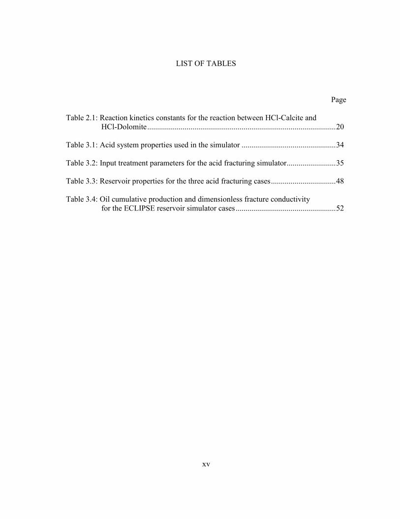
Table 2.1: Reaction kinetics constants for the reaction between HCl-Calcite and HCl-Dolomite ................................................................................................ 20
Table 3.1: Acid system properties used in the simulator ................................................ 34
Table 3.2: Input treatment parameters for the acid fracturing simulator......................... 35
Table 3.3: Reservoir properties for the three acid fracturing cases ................................. 48
Table 3.4: Oil cumulative production and dimensionless fracture conductivity for the ECLIPSE reservoir simulator cases ................................................... 52
1
CHAPTER I
INTRODUCTION
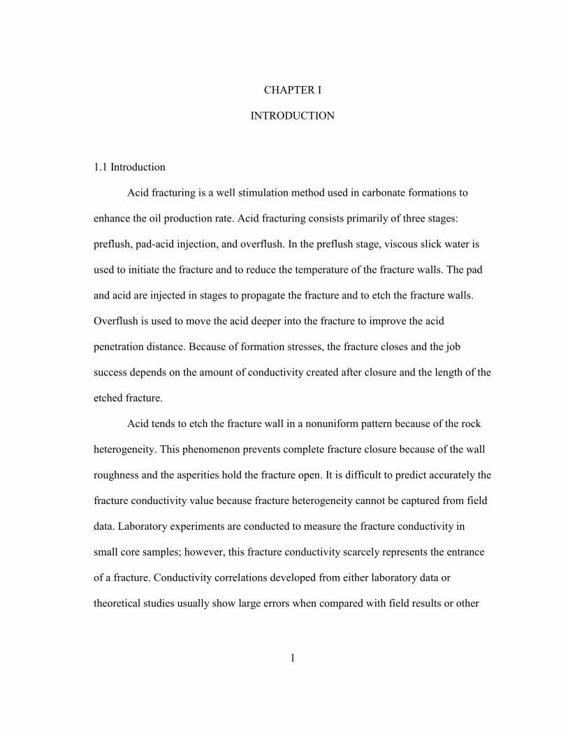
1.1 Introduction
Acid fracturing is a well stimulation method used in carbonate formations to
enhance the oil production rate. Acid fracturing consists primarily of three stages:
preflush, pad-acid injection, and overflush. In the preflush stage, viscous slick water is
used to initiate the fracture and to reduce the temperature of the fracture walls. The pad
and acid are injected in stages to propagate the fracture and to etch the fracture walls.
Overflush is used to move the acid deeper into the fracture to improve the acid
penetration distance. Because of formation stresses, the fracture closes and the job
success depends on the amount of conductivity created after closure and the length of the
etched fracture.
Acid tends to etch the fracture wall in a nonuniform pattern because of the rock
heterogeneity. This phenomenon prevents complete fracture closure because of the wall
roughness and the asperities hold the fracture open. It is difficult to predict accurately the
fracture conductivity value because fracture heterogeneity cannot be captured from field
data. Laboratory experiments are conducted to measure the fracture conductivity in
small core samples; however, this fracture conductivity scarcely represents the entrance
of a fracture. Conductivity correlations developed from either laboratory data or
theoretical studies usually show large errors when compared with field results or other
2
experimental data. In such stochastic processes, it is not unusual to find discrepancies in
terms of stimulation ratio between field results and acid design calculations.
The design of an acid fracturing treatment is accomplished by estimating the
optimum conductivity and acid penetration distance that results in maximum benefit of
the treatment. Design parameters include selecting the fluid types, number of stages,
pumping rate, and injection time. Changing these parameters results in different fracture
geometry, etching patterns, and acid-penetration distance. A complete study of formation
fluid properties, mineralogy and permeability distributions, and formation temperature
should be conducted prior to the stimulation operation. Simulators are usually used to
estimate how these design parameters affect the stimulation job.
1.2 Literature Review
Using acid to stimulate a carbonate formation is not a recent practice. In 1895,
Standard Oil Company used concentrated hydrochloric acid as a stimulation fluid to
enhance oil production from the Lima formation in Ohio. The first observation of the
effects of acid fracturing occurred in 1935. At that time, Schlumberger stimulated a
reservoir by acid injection where the formation was determined to be fractured when the
pressure reached “lifting pressure”. Acid fracturing became an accepted stimulation
method for carbonate reservoirs to improve production not achievable by matrix
treatment alone (Kalfayan, 2007).
Propped fracturing is another stimulation method used in carbonate formations.
In many cases, propped fracturing is preferred over acid fracturing because conductivity

3
is preserved longer. Designing propped fracturing is more convenient and predictable
than acid fracturing because reactive fluids are not used in the process, which makes it
easy to predict the formation conductivity. Many researchers have provided an
application window for each technique but there are no strict guidelines. Acid fracturing
is usually preferred when the formation is shallow and very heterogeneous to maintain
conductivity after fracture closure. One advantage of acid fracturing is the low
probability of job failure because early screenout is not possible in this case.
One of the first acid-fracturing conductivity calculations was performed by
Nierode and Kruk (1973). They stated that conductivity is difficult to predict because of
rock heterogeneity due to the fact that laboratory experiments represent only the
entrance of the fracture. In correlating the calculations and laboratory experimental
results, Nierode and Kruk concluded that conductivity is function of the amount of
dissolved rock (DREC), rock embedment strength (RES), and formation closure stress
(s). The correlation was based on 25 laboratory experiments with small cores that were
cut under tension to produce rough surfaces. The Nierode and Kruk conductivity
correlation is shown in Eqs. 1.1-1.3:
( )…………………………………………...…………………… (1.1)
( ) ………………………………………………...…………. (1.2)
{ ( )
( ) } …………...……. (1.3)
This correlation represents the lower bound of conductivity when compared with
field values as suggested by Nierode and Kruk. Numerous commercial software
4
programs use this correlation where parameters can be easily obtained from field data or
core analysis. Since 1973, several correlations were developed based on theoretical or
empirical background (Gangi, 1978; Walsh, 1981; Gong et al., 1999; Pounik, 2008).
Even though the Nierode and Kruk work is the standard in the oil industry, it fails to
capture the significant impact of formation heterogeneity on fracture conductivity. Deng
et al. (2012) attempted to include the effect of formation heterogeneity in their
theoretical correlation. They stated that permeability and mineralogy distribution are the
reasons for differential etching in carbonate rocks. Three parameters are used to
characterize permeability distribution: the correlation lengths in horizontal (𝞴D,x) and
vertical (𝞴D,z) directions and the normalized standard deviation of permeability (σD). The
correlation length in the x direction has higher value because of the natural bedding in
that direction. The higher the 𝞴D,x , the higher the conductivity because of the fracture
channels that are difficult to close. A high 𝞴D,z results in low conductivity because
fracture-isolated openings contribute less to the flow in the fracture. A high σD means
better width distribution, resulting in harder to close channels, which means better
fracture conductivity. Mineralogy distribution depends on the percentage of calcite and
dolomite in the rock. The higher the percentages of calcite, the more opening are the
channels when the fracture closes, which means higher conductivity. The optimum
percentage for calcite is 50%; however, conductivity decreases for higher calcite
percentages. Rock mechanical properties have an impact on conductivity, especially
Young’s modulus, where higher values result in higher conductivity. Variation in
Poisson’s ratio does not have a significant impact on conductivity; therefore, a typical
5
value of 0.3 is used. The correlations developed are divided into three cases:
permeability distribution, mineralogy distribution, and a competing case between the
two.
To estimate the well productivity improvement, two parameters should be
provided: 1) the ratio of fracture length to drainage radius; and 2) the ratio of fracture
conductivity to the formation permeability (McGuir and Sikora, 1960). Acid penetration
distance in reactive formations ranges from a maximum penetration distance case where
the pad fluid is assumed to control the leakoff rate (reaction rate limit) and a minimum
penetration distance where acid viscosity is assumed to control acid leakoff (fluid loss
limit). Because the reaction rate between hydrochloric acid (HCl) and a carbonate
formation occurs so quickly, the process of rock etching is controlled by the acid mass
transfer to the fracture wall, which is the slower step. Fluid loss additives and acid
retarders are usually added to an acid system to enhance etching performance and acid
penetration distance.
Designing an acid-fracturing job nowadays is performed by using simulators.
Before simulators, analytical solutions of velocity and concentration profiles in 1D or 2D
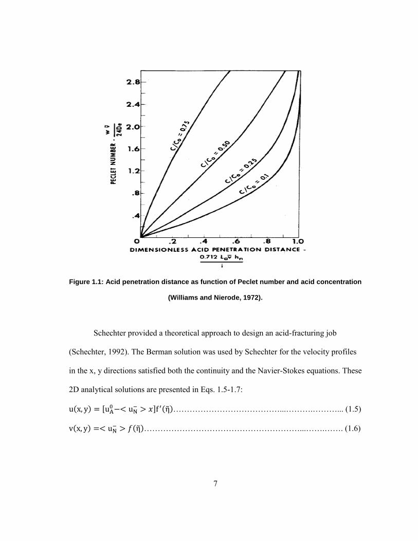
were used and a simple procedure was implemented. Nierode and Williams (1972)
suggested a design procedure to predict stimulation ratio. The procedure began by
calculating acid penetration distance from a chart (Fig.1.1) using Peclet number and a
specific acid concentration value to read the dimensionless acid penetration number. The
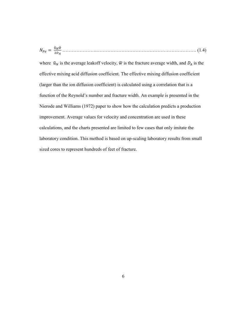
Peclet number, NPe, is given in the equation below:
6
………………….………………………………………………………. (1.4)
where is the average leakoff velocity, is the fracture average width, and is the
effective mixing acid diffusion coefficient. The effective mixing diffusion coefficient
(larger than the ion diffusion coefficient) is calculated using a correlation that is a
function of the Reynold’s number and fracture width. An example is presented in the
Nierode and Williams (1972) paper to show how the calculation predicts a production
improvement. Average values for velocity and concentration are used in these
calculations, and the charts presented are limited to few cases that only imitate the
laboratory condition. This method is based on up-scaling laboratory results from small
sized cores to represent hundreds of feet of fracture.
7
Figure 1.1: Acid penetration distance as function of Peclet number and acid concentration
(Williams and Nierode, 1972).
Schechter provided a theoretical approach to design an acid-fracturing job
(Schechter, 1992). The Berman solution was used by Schechter for the velocity profiles
in the x, y directions satisfied both the continuity and the Navier-Stokes equations. These
2D analytical solutions are presented in Eqs. 1.5-1.7:
u( ) [
] ( )…………………………………...……….………... (1.5)
( ) ( )…………………………………………………...…….……. (1.6)

8
…………………………………..…………..….…………… (1.7)
where u, v are velocities in the x, y directions, is the average velocity inside the
fracture, is the acid injection rate, is the fracture height, and is a dimensionless
number for acid position in a fracture width direction. The acid mass balance equation is
used to calculate concentration as function of the x- direction where the y-direction
concentration values are averaged. The acid mass balance equation and the analytical
solutions are shown in Eqs.1.7-1.8:
( )
( )
……………………………………………....……. (1.8)
∑ (
)
………………………………………....…………...… (1.9)
where are eigenvalues, is the acid concentration, is the average acid
concentration, is the initial acid concentration, and L is the acid penetration distance.
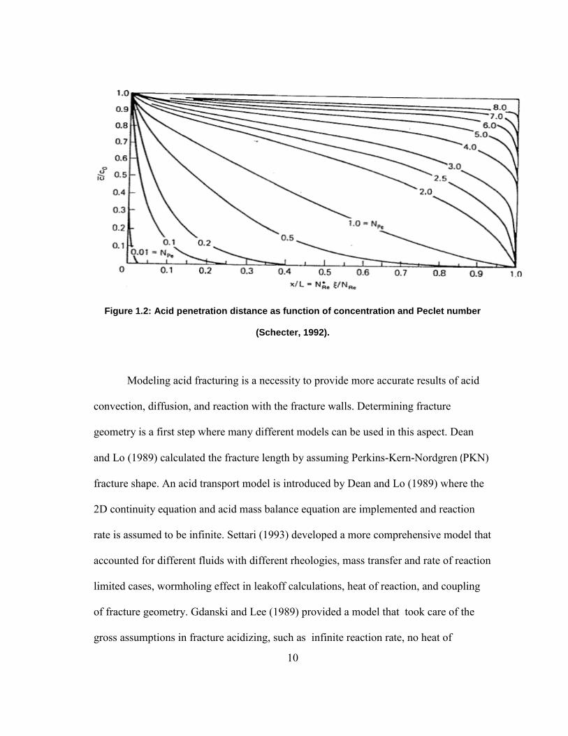
From the solution presented in Figure 1.2 for a Peclet number greater than one, the case
is the fluid loss limit where the fluid completely leaks off before the acid is exhausted.
When the Peclet number is less than one, it is reaction-limit controlled and the acid is
consumed before the fluid leaks off. This analytical solution has a limitation in terms of
Peclet values and Reynolds numbers. In general, the solution assumptions are: laminar
flow and infinite reaction rate while wall roughness and secondary flow effects are
neglected. The length (L) in this case may not be the actual fracture half-length but is the
acid-penetration length that will satisfy the volume balance equation (injection rate =
fluid loss rate). The ideal fracture width is calculated as a function of fracture length (x)

9
where the Terrill (1964) acid solution is used for width calculations. It is found that the
higher the Peclet number, the more distributed is the etching along the fracture. Width
distribution as a function of distance is shown in Eq. 1.10:
( )
[(
)
]…………...……………….………………………. (1.10)
where is the ideal fracture width, is the fluid density, is the formation porosity,
is the total time of acid injection, and is the gravimetric dissolving power. An
equation for an optimum penetration distance is suggested assuming the fracture is
equally etched along its length. The equation used is an analogue to that of the prop
fracture case. Selecting acid viscosity can determine the acid leakoff coefficient; hence,
the acid injection rate and the penetration distance. An issue with acid fracturing design
is the Peclet number that gives optimum penetration distance may not give optimum
uniform etching.
10
Figure 1.2: Acid penetration distance as function of concentration and Peclet number
(Schecter, 1992).
Modeling acid fracturing is a necessity to provide more accurate results of acid
convection, diffusion, and reaction with the fracture walls. Determining fracture
geometry is a first step where many different models can be used in this aspect. Dean
and Lo (1989) calculated the fracture length by assuming Perkins-Kern-Nordgren (PKN)
fracture shape. An acid transport model is introduced by Dean and Lo (1989) where the
2D continuity equation and acid mass balance equation are implemented and reaction
rate is assumed to be infinite. Settari (1993) developed a more comprehensive model that
accounted for different fluids with different rheologies, mass transfer and rate of reaction
limited cases, wormholing effect in leakoff calculations, heat of reaction, and coupling
of fracture geometry. Gdanski and Lee (1989) provided a model that took care of the
gross assumptions in fracture acidizing, such as infinite reaction rate, no heat of
11
reaction, constant average fracture temperature, no convection effect, and single stage
geometry.
The number of pore volumes (PV) to breakthrough is very important in
determining the effect of wormholing. Normally, carbonate formations have small PVs
while dolomite has higher PVs to breakthrough; hence, the effect of wormholing is
significant in carbonate reservoirs, especially in gas fields. Leakoff parameters are
important in the solution of acid penetration distance and acid fracturing conductivity. A
volumetric method introduced by Economides et al. (1994) is used where flow is linear
and wormholes are short. For short wormholes, the wormhole growth is almost linear
with fluid flux. Parameters are varied in experimental work to account for wormholing,
including acid concentration, injection rates, and temperature. Pressure drop is
measured against PV and found to be almost linear, which means that wormhole growth
is almost linear in the case of carbonates. In dolomite, the growth is not linear and the
PV value can be as high as 50. Experiments showed that there is an optimum value for
injection rate where PV is at minimum. It is safe to increase the injection rate because
the increase in PV is gradual and small. Assuming a constant injection rate and constant
growth velocity of wormholes, the length of the wormhole is correlated with the
injection rate. Formation zones are divided into filter cake, Cw, wormhole and invaded
zone, Cv, and compressed reservoir zone, Cc, as shown in Figure 1.3. Wormholes will
affect only the fluid loss in the invaded zones and pressure drop is assumed to be
negligible in wormholes when compared with the matrix. For those reasons, the only
change that accounts for including wormholing is in the viscous fluid loss coefficient
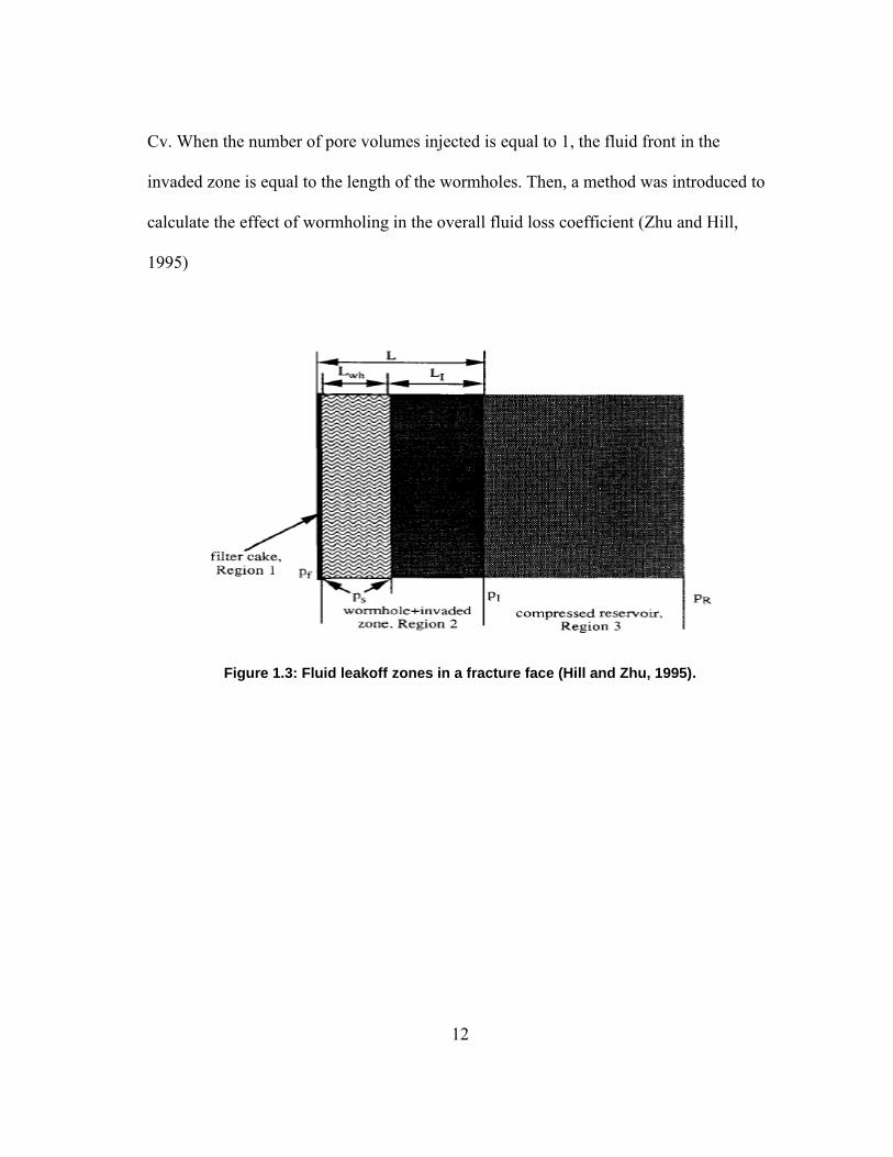
12
Cv. When the number of pore volumes injected is equal to 1, the fluid front in the
invaded zone is equal to the length of the wormholes. Then, a method was introduced to
calculate the effect of wormholing in the overall fluid loss coefficient (Zhu and Hill,
1995)
Figure 1.3: Fluid leakoff zones in a fracture face (Hill and Zhu, 1995).
13
1.3 Research Objectives
An acid fracturing simulator that uses a 3D solution of velocity, pressure, and
concentration profiles has already been developed. The approach and algorithm of this
simulator is illustrated by Mou (2010) and an analytical validation and some
development of the model has been presented by Oeth (2013). The correlation used to
evaluate acid fracture conductivity was theoretically developed by Deng et al. (2012).
The main objectives of my research are as follows:
1- Provide a detailed study of the algorithm and equations used in the simulator to
make it convenient for other researchers to further develop the simulator.
2- Use the simulator to perform parametric studies to evaluate the effect of fluids
and formation properties on fracture conductivity and acid penetration distance.
The simulator output is imported to the ECLIPSE ™ reservoir simulator to
evaluate production enhancement for different cases and to be able to draw a
solid conclusion about fracture treatment performance.
3- Provide a summary of simulator limitations and identify other hydraulic,
mechanical, thermal, and geochemical phenomena that should be included to
improve the model’s accuracy. Some input data cause the simulator to
prematurely terminate without completing the run. This issue is further
investigated in this research.
14
CHAPTER II
MODEL THEORETICAL APPROACH
2.1 Model Algorithm
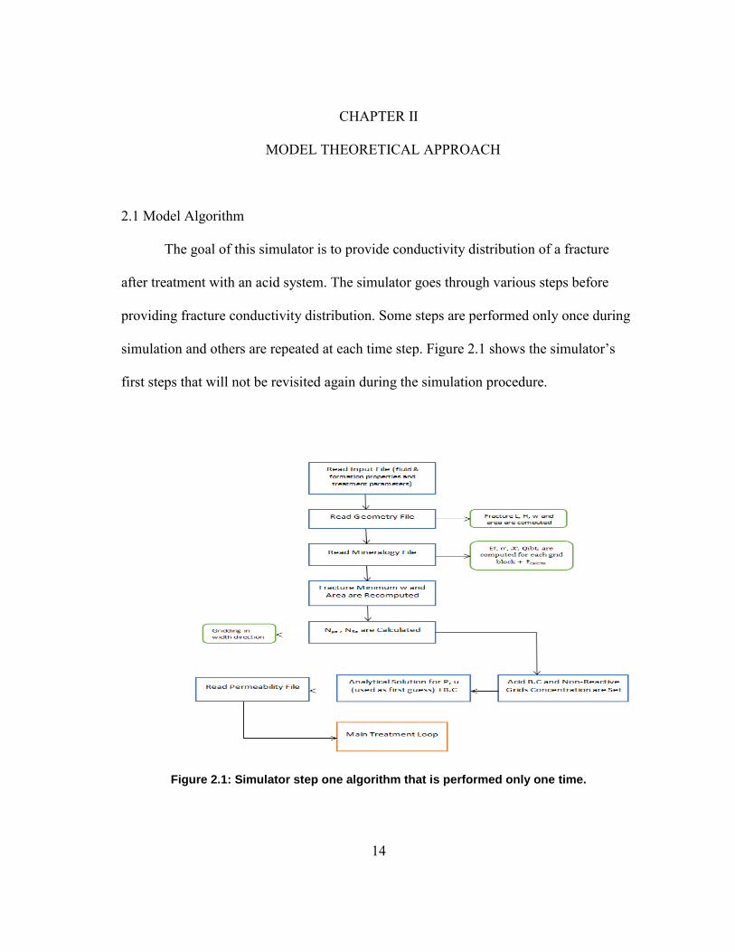
The goal of this simulator is to provide conductivity distribution of a fracture
after treatment with an acid system. The simulator goes through various steps before
providing fracture conductivity distribution. Some steps are performed only once during
simulation and others are repeated at each time step. Figure 2.1 shows the simulator’s
first steps that will not be revisited again during the simulation procedure.
Figure 2.1: Simulator step one algorithm that is performed only one time.

15
The user has to provide input data that includes fluid and formation properties in
addition to treatment parameters. The simulator then reads the fracture width distribution
(geometry), which has to be provided by other hydraulic propagation models. The
number of grids in the fracture height and fracture length depends on the precision of
width distribution provided by the gridding system of the fracture propagation model.
Fracture height and length are considered to be constant while fracture width will change
during the acid injection. Formations can consist of calcite, dolomite, and nonreactive
minerals. The simulator reads mineralogy distribution and computes the reaction rate
constant, order of reaction, volume dissolving power, and the pore volume to
breakthrough value for each grid cell. The percentage of calcite in a fracture is evaluated
and used in the Mou-Deng (2012) conductivity correlation. Fracture average width and
area are calculated again where nonreactive grids are excluded this time. Gridding in the
width direction is performed by calculating the Peclet number (Npe) and based on that
value, the number of grids are determined. The simulator imposes the restriction that the
concentration at the fracture inlet and at the nonreactive grid cells is equal to the initial
concentration and will not change during treatment. Before moving to the Navier-Stokes
and continuity equations, an analytical solution for velocity in the length direction (ux)
and pressure is provided as a first-guess solution. Before moving to main treatment loop,
the simulator reads permeability distribution, which affects the fracture leakoff
properties.
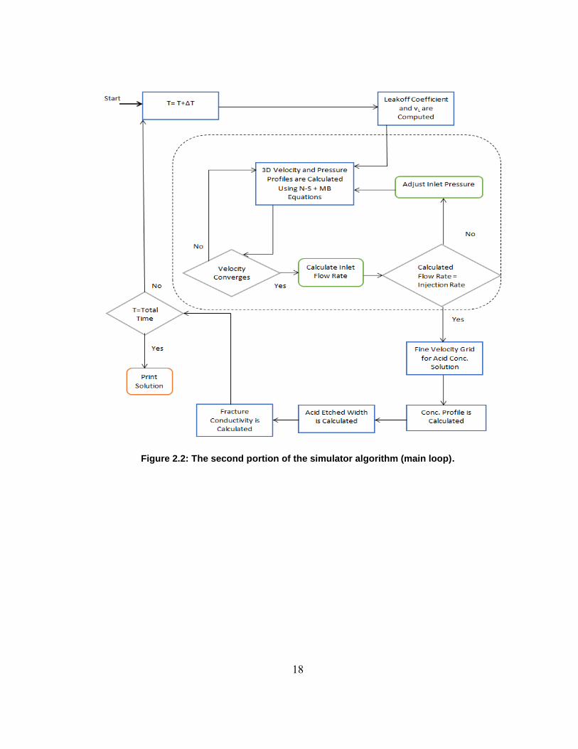
The main treatment loop is performed at each time step until reaching the end of
treatment time (Fig. 2.2). The leakoff coefficient for each gird cell at the fracture face is
16
calculated by using the two models. As long as the acid front is beyond the grid blocks
in the fracture face, the leakoff coefficient without the wormhole effect is considered;
otherwise, the wormhole effect should be included. Leakoff velocity through the fracture
walls can be estimated and penetration distance afterward can be easily determined. The
leakoff velocity is considered as a velocity boundary condition in the width direction (vy)
and can change at each time step. Subsequently, the simulator moves to the continuity
and momentum balance equations (Navier-Stokes) to solve for velocity and pressure in
3D. The following steps are performed when the simulator reaches this point (Oeth,
2013):
1) Begin with a guessed velocity profile.
2) Calculate the pressure coefficient matrix based on continuity and the momentum
balance equations, and solve for pressure by inverting this matrix.
3) Use the three momentum equations to calculate the velocity profile using
pressure values in Step 2.
4) Compare the calculated velocity with the guessed velocity, and if the velocity
converges, then terminate the solution; otherwise, restart the algorithm with the
new velocity profile.
After completing these steps, a 3D pressure and velocity profile inside of the fracture
are obtained. The velocity profile at the entrance is used to calculate the inlet injection
rate and if it is within 10% of the user-specified injection rate, then the simulator moves
to the acid concentration profile; otherwise, inlet pressure values will be adjusted and the
continuity and momentum balance equations will be evaluated again to obtain a velocity
17
profile that satisfies the inlet injection rate. The velocity profile is used for 3D
calculations of the concentration profile inside of the fracture. The concentration profile
is used to calculate the amount of acid that diffuses through the fracture wall and the
concentration of leaked off fluid. An etching profile for each grid cell at the fracture
faces is calculated where diffusion and leakoff are considered to be the only methods to
reach the fracture wall. These etching profile and fracture statistical parameters are
imported into the Mou-Deng correlation file to evaluate the conductivity distribution.
The water flushing effect after acid injection is also included in the simulator where the
acid concentration in the flushed zone is assumed to be zero. The results are printed in
one minute intervals to show how the solutions change with time. The Tecplot Focus ™
program is used to view the results in 2D and 3D. Figure 2.2 shows the flow chart of the
approach.
18
Figure 2.2: The second portion of the simulator algorithm (main loop).
19
2.2 Model Equations
Some of the equations used in this model are fundamental and based on physics
laws such as conservation of mass and momentum. These equations are differential
equations and can be solved numerically or analytically. Most of analytical solutions are
based on many assumptions and simplifications, which limit the model and cause it to be
less representative of the real world. In this model, a numerical solution using SIMPLE
(Semi-Implicit Method for Pressure Linked Equations) is implemented where averaging
in 1D is no longer needed. This section introduces most of the equations used in the
model. For model validation and comparison with analytical solutions, the reader may
refer to the Oeth (2013) dissertation.
2.2.1 Reaction Equations
The reaction between an acid and a fracture is heterogeneous where acid has to
diffuse to the rock surface to react with the minerals. The diffusion flux ( ) depends on
the acid concentration gradient (
) and the diffusion coefficient ( ) as expressed by
Fick’s law (Eq.2.1).
………………………...……..……………………………………… (2.1)
If diffusion is slow when compared with the reaction rate, it becomes the rate
determining step and the reaction is called diffusion limited. If the diffusion is faster than
the reaction rate, then reaction becomes the rate determining step and the reaction is
called reaction limited. Because HCl reactions are so fast, once the molecules collide
20
with each other, a product will form; hence, an acid reaction, which in this case is
diffusion limited.
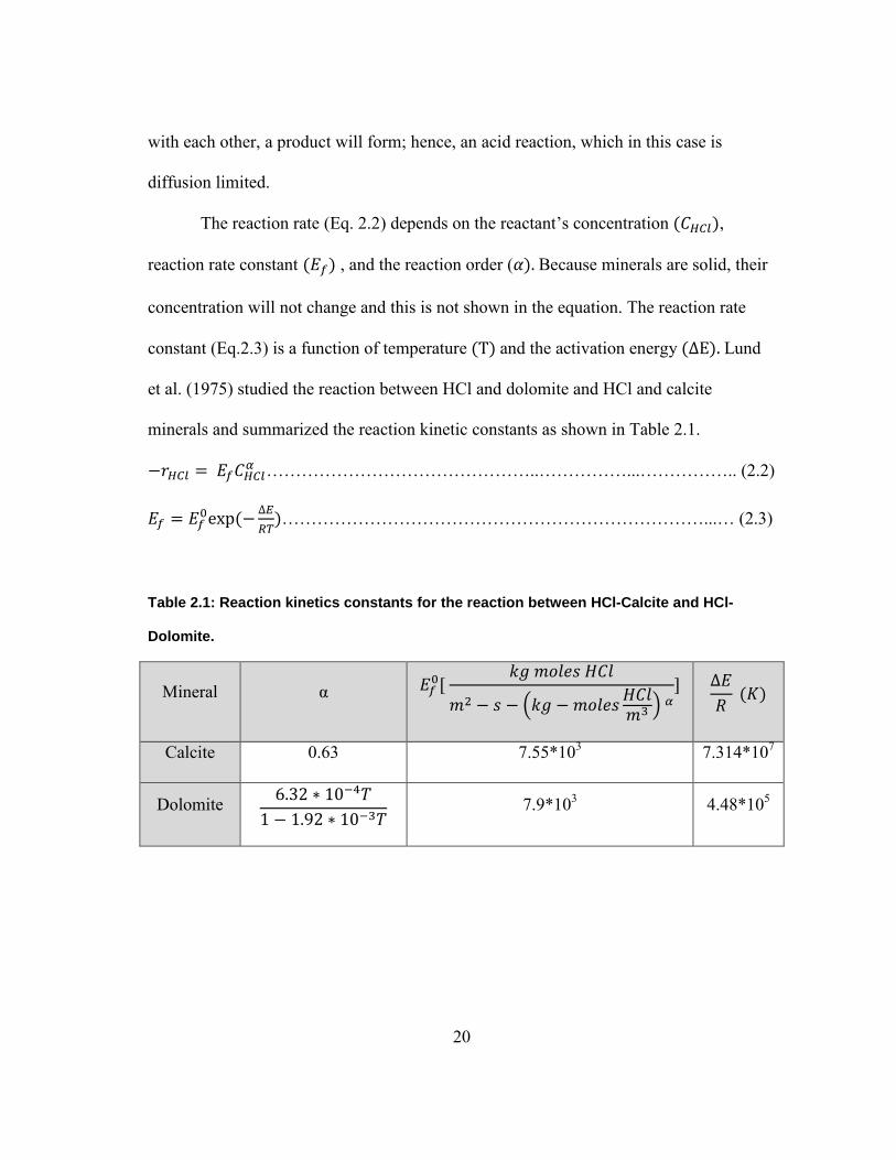
The reaction rate (Eq. 2.2) depends on the reactant’s concentration ( ),
reaction rate constant ( ) , and the reaction order (𝛼). Because minerals are solid, their
concentration will not change and this is not shown in the equation. The reaction rate
constant (Eq.2.3) is a function of temperature (T) and the activation energy (∆E) Lund
et al. (1975) studied the reaction between HCl and dolomite and HCl and calcite
minerals and summarized the reaction kinetic constants as shown in Table 2.1.
………………………………………..……………...…………….. (2.2)
(
∆
)………………………………………………………………...… (2.3)
Table 2.1: Reaction kinetics constants for the reaction between HCl-Calcite and HCl-
Dolomite.
Mineral α [
( )
] ∆
( )
Calcite 0.63 7.55*103 7.314*107
Dolomite
7.9*103 4.48*105

21
A less complicated way to calculate the amount of etching is by calculating the
dissolving power ( ) introduced by Williams, Gidley, and Schechter (1979). This
calculation is based on the assumption that the reaction between an acid and a mineral is
complete. Gravimetric dissolving power (𝛽) should be calculated first (Eq. 2.4), which
depends on the stoichiometric coefficient (𝜈) and molecular weight (MW) of the
reactants. The stoichiometric coefficients in this case can be computed by balancing the
reaction between the HCl and the minerals (Eq. 2.6-2.7). When the acid concentration is
less than 100%, then this concentration should be multiplied by 𝛽. By calculating the
dissolving power, computing the volume of acid needed to dissolve a certain amount or
volume of minerals becomes easy. Weak acids are treated differently because they do
not react completely; hence, knowledge of equilibrium composition is inevitable.
𝛽
……………………………...…………………………...…… (2.4)
𝛽(
)………………………………………………...………….….…..… (2.5)
……………………………………………. (2.6)
( ) ………………………. (2.7)
2.2.2 Analytical Solutions for Pressure and Velocity inside the Fracture
Before numerically solving for velocity and pressure in 3D, a first- supposition
analytical solution is used. This solution (Eq.2.8) is obtained by simplifying momentum
and continuity equations into a 1D solution for velocity. This solution is applied for both
Newtonian fluids and non-Newtonian fluids that follow the power low model (Eq.2.11),
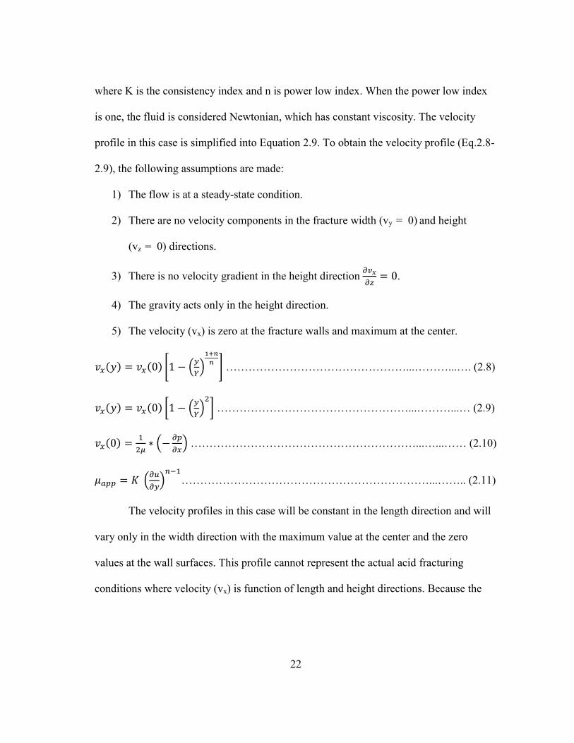
22
where K is the consistency index and n is power low index. When the power low index
is one, the fluid is considered Newtonian, which has constant viscosity. The velocity
profile in this case is simplified into Equation 2.9. To obtain the velocity profile (Eq.2.8-
2.9), the following assumptions are made:
1) The flow is at a steady-state condition.
2) There are no velocity components in the fracture width (vy = 0) and height
(vz = 0) directions.
3) There is no velocity gradient in the height direction
.
4) The gravity acts only in the height direction.
5) The velocity (vx) is zero at the fracture walls and maximum at the center.
( ) ( ) [ (
)
] …………………………………………...………...…. (2.8)
( ) ( ) [ (
)
] ……………………………………………...………...… (2.9)
( )
(
) ……………………………………………………...…...…… (2.10)
(
)
…………………………………………………………...…….. (2.11)
The velocity profiles in this case will be constant in the length direction and will
vary only in the width direction with the maximum value at the center and the zero
values at the wall surfaces. This profile cannot represent the actual acid fracturing
conditions where velocity (vx) is function of length and height directions. Because the
23
fracture walls are porous, the velocity component in the width direction (vy) cannot be
ignored; however, this solution can be useful as first deduction and input into the Navier-
Stokes equations.
A first conjecture as a solution for pressure is provided by assuming that the
pressure gradient is constant along the length direction and there is no pressure gradient
in other directions (Eq.2.12). The pressure value at the fracture entrance Pin is calculated
by using Equation 2.13. This calculated value is then populated to all direction as a first
deduction and input into the Navier-Stokes equations.
(
∆
) ∆
……………………………...…………….….. (2.12)
[
( )
]
…………………………………………………...…..…… (2.13)
2.2.3 Leakoff Coefficient
The leakoff coefficient calculation is very important in designing hydraulic and
acid fracturing processes (Ben-Naceur et al., 1989). The shape of the fracture and the
penetration distance are both affected by this value. Also, this value can determine the
efficiency of a fracturing job, which is the ratio of the pumped fluids volume to the
fracture volume. A high-leakoff coefficient can cause premature job failure because the
pressure cannot build up to the fracture pressure. The leakoff coefficient consists of three
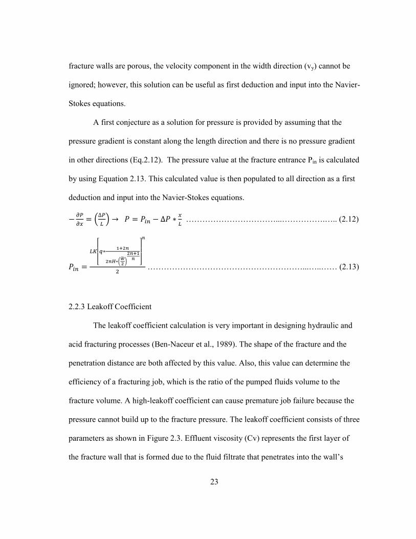
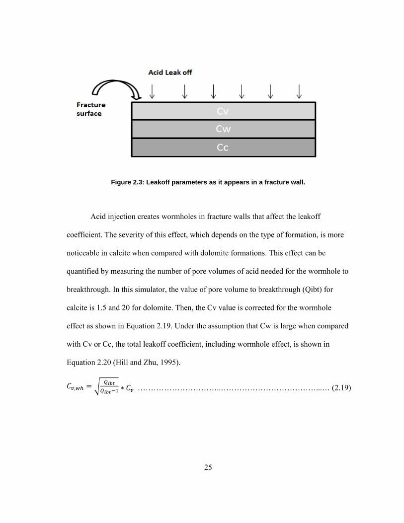
parameters as shown in Figure 2.3. Effluent viscosity (Cv) represents the first layer of
the fracture wall that is formed due to the fluid filtrate that penetrates into the wall’s

24
pores. The second layer exists because of the wall building (Cw) due to the accumulation
of fluid filtrate during injection. The third layer represents the reservoir fluid viscosity
and compressibility (Cc). The effluent and reservoir fluid coefficients can be calculated
from the reservoir and fluid properties (Eq. 2.14-2.15) while the wall buildup coefficient
can be determined experimentally (Eq. 2.16). There are several methods available to
combine the three coefficients into one leakoff coefficient. One method combines Cv
and Cc as shown in Equation 2.17 and compares the value with Cw and the lesser
coefficient is used as total coefficient. Another method combines the total pressure drop
contribution of each coefficient that leads to Equation 2.18. (Recent Advances in
Hydraulic Fracturing, 1989)
( ∆
)
…………………………………………….…………….. (2.14)
∆ (
)
…………………………………………………..……. (2.15)
∆
………………………………………………………….……. (2.16)
(
) ………………………………………………………….…… (2.17)
[
(
)]
…………………………………………………….. (2.18)
25
Figure 2.3: Leakoff parameters as it appears in a fracture wall.
Acid injection creates wormholes in fracture walls that affect the leakoff
coefficient. The severity of this effect, which depends on the type of formation, is more
noticeable in calcite when compared with dolomite formations. This effect can be
quantified by measuring the number of pore volumes of acid needed for the wormhole to
breakthrough. In this simulator, the value of pore volume to breakthrough (Qibt) for
calcite is 1.5 and 20 for dolomite. Then, the Cv value is corrected for the wormhole
effect as shown in Equation 2.19. Under the assumption that Cw is large when compared
with Cv or Cc, the total leakoff coefficient, including wormhole effect, is shown in
Equation 2.20 (Hill and Zhu, 1995).
√
…………………………..………………………………...… (2.19)
26
√
(
)
………………………………………………………….…….. (2.20)
The leakoff velocity at the fracture wall is calculated (Eq.2.21) and used as a
boundary condition later in Navier-Stokes equations. By volume balance (volume
injected = leakoff volume), the penetration distance can be determined using Equation
2.22. After this distance, there is no acid convection or diffusion, which means this part,
will have zero conductivity after fracture closure.
√ ……………………………………………………………………….…… (2.21)
……………………………………………………………………...……. (2.22)
2.2.4 Navier Stokes Equations
To solve for three velocity components (vx, vy, vz) and pressure (P) inside the
fracture, four equations are need. These equations are three momentum balances in each
coordinate (Eqs. 2.24-2.26) and one continuity equation (Eq.2.23). These equations are
further simplified by making the following assumptions:
1) A steady-state condition exists, which means no property change will occur with
time ( )
.
2) Newtonian fluids are assumed for these equations, but the model can handle non-
Newtonian fluids as well (Oeth, 2013).
3) Gravity effect is neglected ( ).
27
4) Density is constant (incompressible fluid).
( )
( )
( )
………………………………………….……..... (2.23)
(
)
(
) ......…. (2.24)
(
)
(
) ......… (2.25)
(
)
(
) …........ (2.26)
Boundary conditions are needed to solve the differential equations, and these
boundary conditions are as follows:
1) At the inlet, the injection rate must be equal to the summation of volumetric flux
across the fracture inlet area.
∫ | ………………………………………………......…….. (2.27)
2) At the outlet, the pressure at the end of fracture is equal to outlet pressure.
| ………………………………………………………......…… (2.28)
3) On the fracture surfaces, the velocity component in the fracture length and height
directions are zero but the velocity in the width direction is equal to leakoff
velocity.
| ………………………………………………………......…. (2.29)
| …………………………………………………...…...……. (2.30)
| ………………………………………………...………...... (2.31)
28
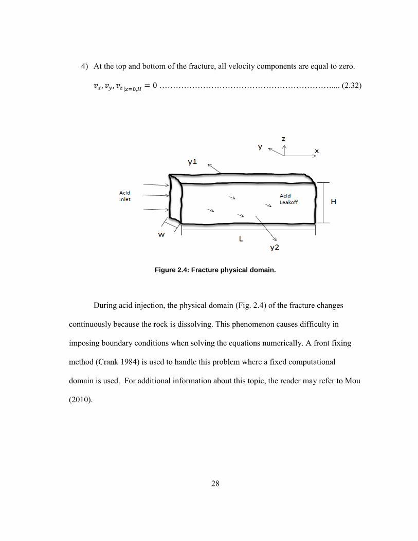
4) At the top and bottom of the fracture, all velocity components are equal to zero.
| ……………………………………………………….... (2.32)
Figure 2.4: Fracture physical domain.
During acid injection, the physical domain (Fig. 2.4) of the fracture changes
continuously because the rock is dissolving. This phenomenon causes difficulty in
imposing boundary conditions when solving the equations numerically. A front fixing
method (Crank 1984) is used to handle this problem where a fixed computational
domain is used. For additional information about this topic, the reader may refer to Mou
(2010).

29
2.2.5 Acid Balance Equation and Etched Width Calculation
Solving the mass balance equation (Eq. 2.33) for acid will provide the
concentration profile in 3D when convection in all directions is assumed. The velocity
profile from the Navier-Stokes equations is used as input into the acid balance equation.
Diffusion is assumed to be only in the width direction where diffusion in other directions
is neglected. In this case, the acid concentration is a function of time and space.
(
)………………………………….. (2.33)
The following boundary conditions are implemented to solve for acid mass
balance numerically:
1) Initial condition, at t = 0, there is no acid inside the fracture.
( ) …………………………………………………....…. (2.34)
2) At the inlet, the acid is live and no reaction has begun.
( ) …………………………………………………...… (2.35)
3) At the top and bottom, no acid concentration gradient is assumed.
| …………………………………………………...……… (2.36)
4) At the fracture surfaces, the rate of acid diffusion is equal to the rate of the
acid reaction.
( )
( )| ……………………..…...... (2.37)
Solving the concentration profile will provide the acid concentration that will
react with fracture minerals. There are two methods for transporting the acid to the
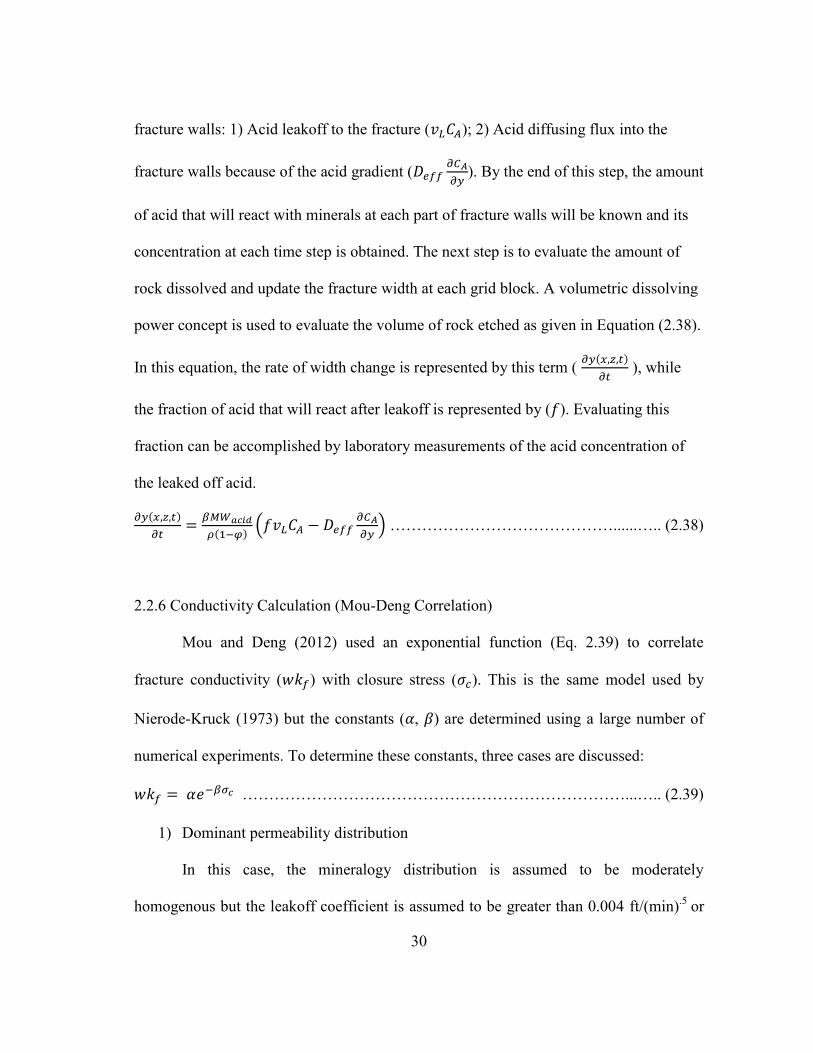
30
fracture walls: 1) Acid leakoff to the fracture ( ); 2) Acid diffusing flux into the
fracture walls because of the acid gradient (
). By the end of this step, the amount
of acid that will react with minerals at each part of fracture walls will be known and its
concentration at each time step is obtained. The next step is to evaluate the amount of
rock dissolved and update the fracture width at each grid block. A volumetric dissolving
power concept is used to evaluate the volume of rock etched as given in Equation (2.38).
In this equation, the rate of width change is represented by this term ( ( )
), while
the fraction of acid that will react after leakoff is represented by ( ). Evaluating this
fraction can be accomplished by laboratory measurements of the acid concentration of
the leaked off acid.
( )
( )(
) ……………………………………......….. (2.38)
2.2.6 Conductivity Calculation (Mou-Deng Correlation)
Mou and Deng (2012) used an exponential function (Eq. 2.39) to correlate
fracture conductivity ( ) with closure stress ( ). This is the same model used by
Nierode-Kruck (1973) but the constants (𝛼, 𝛽) are determined using a large number of
numerical experiments. To determine these constants, three cases are discussed:
𝛼 ………………………………………………………………...….. (2.39)
1) Dominant permeability distribution
In this case, the mineralogy distribution is assumed to be moderately
homogenous but the leakoff coefficient is assumed to be greater than 0.004 ft/(min).5 or

31
approximately 0.001 ft/(min).5. Because the leakoff is high and the minerals are either
100% calcite or 100% dolomite, the permeability effect will prevail. In their correlations,
they used the average fracture width (Eq.2.40-2.41) instead of the ideal width (rock
dissolved volume over fracture area).
( ) ( ) ………………….....……… (2.40)
( ) ( ) …………..………………… (2.41)
To begin with, the conductivity at zero closure stress ( ) should be evaluated (Eq.
2.42). This value is incorporated into 𝛼 with other statistical parameters for the
permeability distribution ( ), while Young’s modulus (E) is incorporated
into 𝛽 (Eqs. 2.43-2.44).
( ) [ ( ( ( )) ( (
)))√ ]
…...…...…. (2.42)
𝛼 ( ) [ ( )
(( ) )
]
……………………. (2.43)
𝛽 [ ( ) ( )] ……………………………...…….. (2.44)
2) Dominant mineralogy distribution
In this case, the leakoff coefficient is assumed to be less than 0.004 ft/(min).5 and
both the dolomite and calcite minerals exist in the formation. The percentage of calcite is
needed in the correlation while the permeability distribution statistical parameters are no
longer used in the correlations (Eqs. 2.45-2.47).

32
( ) [ ( ) ][
]
……..….... (2.45)
𝛼 ( ) ( ) ……………………………………………. (2.46)
𝛽 [ ] …………………………………….. (2.47)
3) Competing between mineralogy and permeability distributions
In this case, the leakoff coefficient is medium; approximately 0.001 ft/(min).5,
and both minerals exist in the formation. The conductivity correlations for this case are
shown in Equations 2.48–2.50:
( ) [ ( ( ( )) ( (
)))√ ] [ ]
…………………………………………...….. (2.48)
𝛼 ( ) [ ( )
] ……………………......…. (2.49)
𝛽 [ ( ) ( )] …………………………………... (2.50)

33
CHAPTER III
PARAMETRIC STUDY
The acid fracturing model is constructed to be able to predict the actual behavior
of reactive fluids inside of a fracture. Conductivity and penetration distance for various
treatment conditions can be obtained from the simulator. The conductivity and
penetration distance have a large impact on the production improvement of a fractured
well. In this section, different parameters will be tested to detect the effect of each
parameter on conductivity and penetration distance. To run the simulator, a fracture
domain should be created. In this case, a PKN geometry model is generated and will be
used for the majority of the cases. This geometry has an elliptical shape at the wellbore
entrance with maximum width at the centerline and zero width at the top and bottom
(Fig. 3.1)
Figure 3.1: A PKN geometry domain.
34
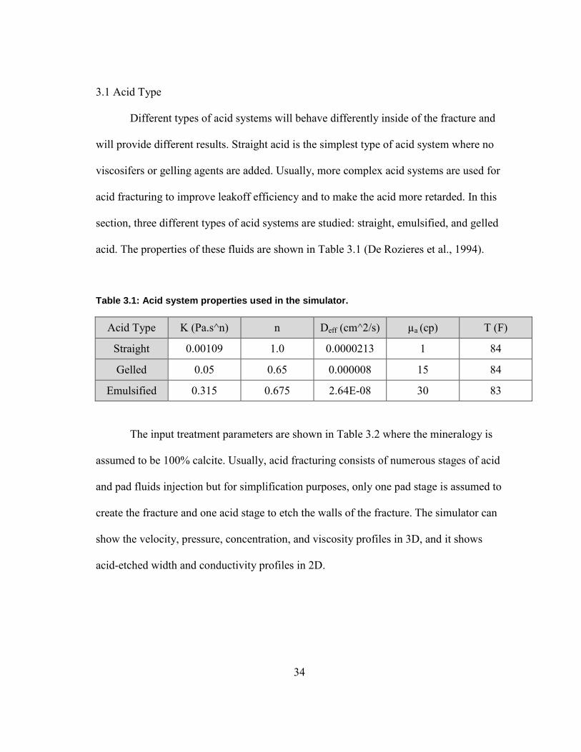
3.1 Acid Type
Different types of acid systems will behave differently inside of the fracture and
will provide different results. Straight acid is the simplest type of acid system where no
viscosifers or gelling agents are added. Usually, more complex acid systems are used for
acid fracturing to improve leakoff efficiency and to make the acid more retarded. In this
section, three different types of acid systems are studied: straight, emulsified, and gelled
acid. The properties of these fluids are shown in Table 3.1 (De Rozieres et al., 1994).
Table 3.1: Acid system properties used in the simulator.
Acid Type K (Pa.s^n) n Deff (cm^2/s) µa (cp) T (F)
Straight 0.00109 1.0 0.0000213 1 84
Gelled 0.05 0.65 0.000008 15 84
Emulsified 0.315 0.675 2.64E-08 30 83
The input treatment parameters are shown in Table 3.2 where the mineralogy is
assumed to be 100% calcite. Usually, acid fracturing consists of numerous stages of acid
and pad fluids injection but for simplification purposes, only one pad stage is assumed to
create the fracture and one acid stage to etch the walls of the fracture. The simulator can
show the velocity, pressure, concentration, and viscosity profiles in 3D, and it shows
acid-etched width and conductivity profiles in 2D.
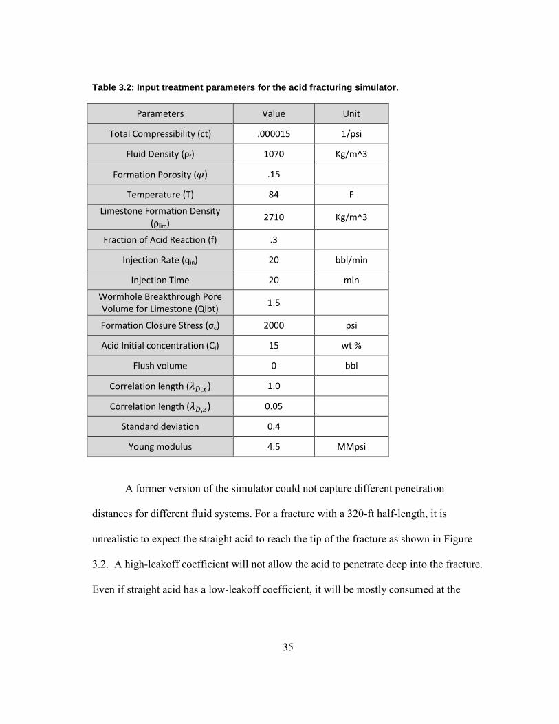
35
Table 3.2: Input treatment parameters for the acid fracturing simulator.
Parameters Value Unit
Total Compressibility (ct) .000015 1/psi
Fluid Density (ρf) 1070 Kg/m^3
Formation Porosity ( ) .15
Temperature (T) 84 F
Limestone Formation Density (ρlim)
2710 Kg/m^3
Fraction of Acid Reaction (f) .3
Injection Rate (qin) 20 bbl/min
Injection Time 20 min
Wormhole Breakthrough Pore Volume for Limestone (Qibt)
1.5
Formation Closure Stress (σc) 2000 psi
Acid Initial concentration (Ci) 15 wt %
Flush volume 0 bbl
Correlation length ( ) 1.0
Correlation length ( ) 0.05
Standard deviation 0.4
Young modulus 4.5 MMpsi
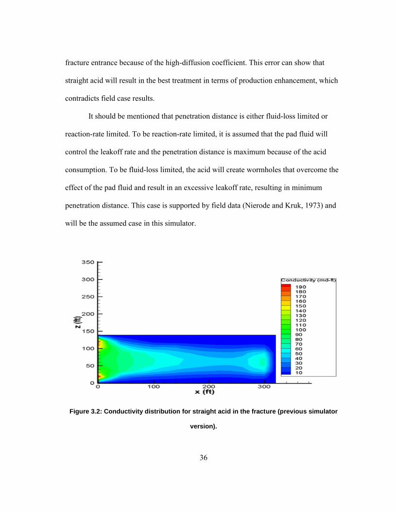
A former version of the simulator could not capture different penetration
distances for different fluid systems. For a fracture with a 320-ft half-length, it is
unrealistic to expect the straight acid to reach the tip of the fracture as shown in Figure
3.2. A high-leakoff coefficient will not allow the acid to penetrate deep into the fracture.
Even if straight acid has a low-leakoff coefficient, it will be mostly consumed at the
36
fracture entrance because of the high-diffusion coefficient. This error can show that
straight acid will result in the best treatment in terms of production enhancement, which
contradicts field case results.
It should be mentioned that penetration distance is either fluid-loss limited or
reaction-rate limited. To be reaction-rate limited, it is assumed that the pad fluid will
control the leakoff rate and the penetration distance is maximum because of the acid
consumption. To be fluid-loss limited, the acid will create wormholes that overcome the
effect of the pad fluid and result in an excessive leakoff rate, resulting in minimum
penetration distance. This case is supported by field data (Nierode and Kruk, 1973) and
will be the assumed case in this simulator.
Figure 3.2: Conductivity distribution for straight acid in the fracture (previous simulator
version).
37
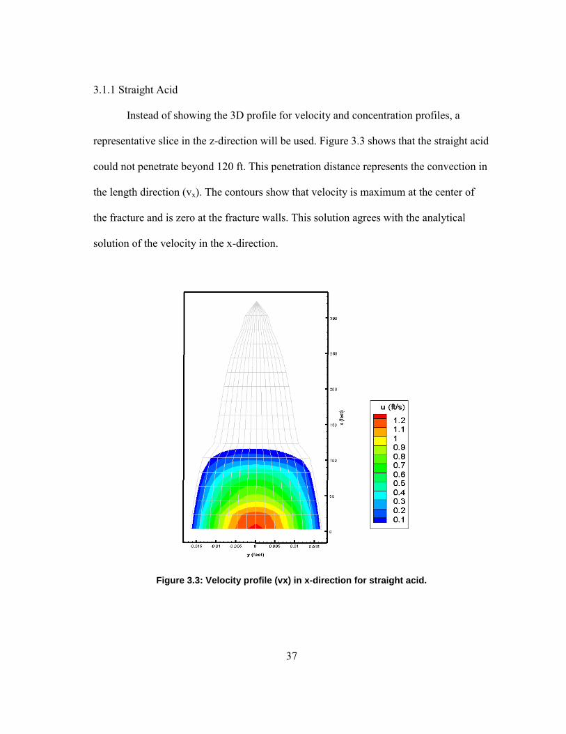
3.1.1 Straight Acid
Instead of showing the 3D profile for velocity and concentration profiles, a
representative slice in the z-direction will be used. Figure 3.3 shows that the straight acid
could not penetrate beyond 120 ft. This penetration distance represents the convection in
the length direction (vx). The contours show that velocity is maximum at the center of
the fracture and is zero at the fracture walls. This solution agrees with the analytical
solution of the velocity in the x-direction.
Figure 3.3: Velocity profile (vx) in x-direction for straight acid.

38
Figure 3.4 shows the velocity profile in the fracture width direction (vy). Velocity
is zero at the center of the fracture and reaches maximum at the fracture walls because of
acid leakoff. An analytical solution of velocity in the y-direction with a leaky channel
supports this numerical solution. Because of the leakoff effect, the profile reaches up to
120 ft and there is no convection beyond that distance.
Figure 3.5 shows the concentration profile for straight acid where concentration
at the inlet and middle of fracture is almost the same as the initial concentration. Toward
the fracture walls and at the end of the profile, the concentration decreases but never
reaches zero. All of the cases run in the simulator have a Peclet number greater than
one, which means that the acid will leakoff before it is consumed completely (fluid loss
limit cases).

39
Figure 3.4: Velocity profile (vy) in y-direction for straight acid.
Figure 3.5: Straight acid concentration profile.

40
Rock etching volume is expected to decrease as the acid travel further into the
fracture as presented in Figure 3.6. Straight acid has higher etching potential when
compared with other fluid systems because of the extremely high diffusion coefficient.
However, straight acid is expected to travel less distance inside of the fracture because of
the low effluent viscosity, resulting in a higher overall leakoff coefficient; and hence, a
higher leakoff rate.
Figure 3.6: Straight acid etched width profile.
41
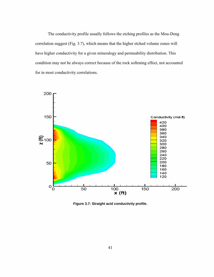
The conductivity profile usually follows the etching profiles as the Mou-Deng
correlation suggest (Fig. 3.7), which means that the higher etched volume zones will
have higher conductivity for a given mineralogy and permeability distribution. This
condition may not be always correct because of the rock softening effect, not accounted
for in most conductivity correlations.
Figure 3.7: Straight acid conductivity profile.
42
3.1.2 Gelled Acid
Gelled acid is simulated in this case where the gelling agent is added to the HCl.
Gelled acid has been used in the industry and proved to be more effective for acid
fracturing. Crowe et al. (1981) investigated different gelling agents in terms of stability,
efficiency, and condition after spending. The study provided the concentration and
temperature at which some gelling agents will be more stable. Also, the potential of
various gelling agents was tested in their study where xanthan polymers showed the
greatest overall potential. The viscosity of gelled acid is several times greater than the
viscosity of straight acid; however, the diffusion coefficient of gelled acid is less than the
straight acid diffusion coefficient, which decreases the amount of acid flux to the
fracture walls. Laboratory experiments with a gelled acid show a lower etching potential
when compared with straight acid etching.. Simulating the gelled acid case showed that
the acid convection can reach up to 240 ft inside of the fracture (Fig. 3.8). This
penetration distance is almost double the penetration distance of a straight acid,
indicating an efficiency improvement in leakoff behavior.
43
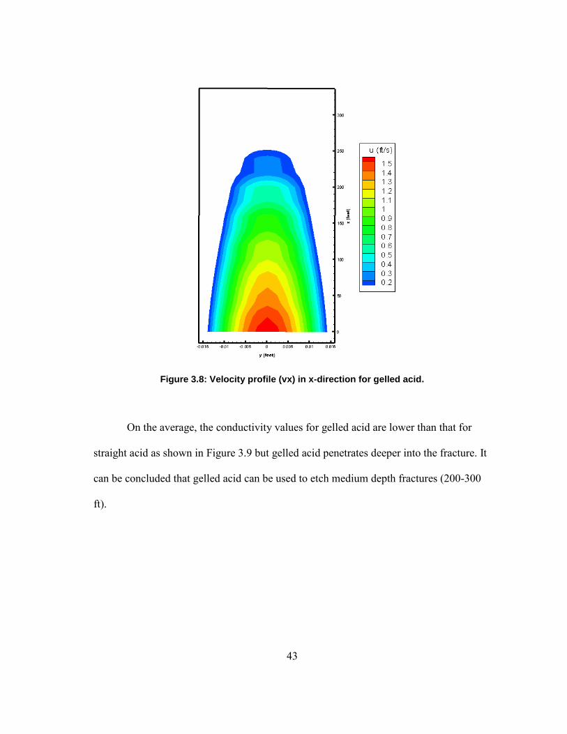
Figure 3.8: Velocity profile (vx) in x-direction for gelled acid.
On the average, the conductivity values for gelled acid are lower than that for
straight acid as shown in Figure 3.9 but gelled acid penetrates deeper into the fracture. It
can be concluded that gelled acid can be used to etch medium depth fractures (200-300
ft).
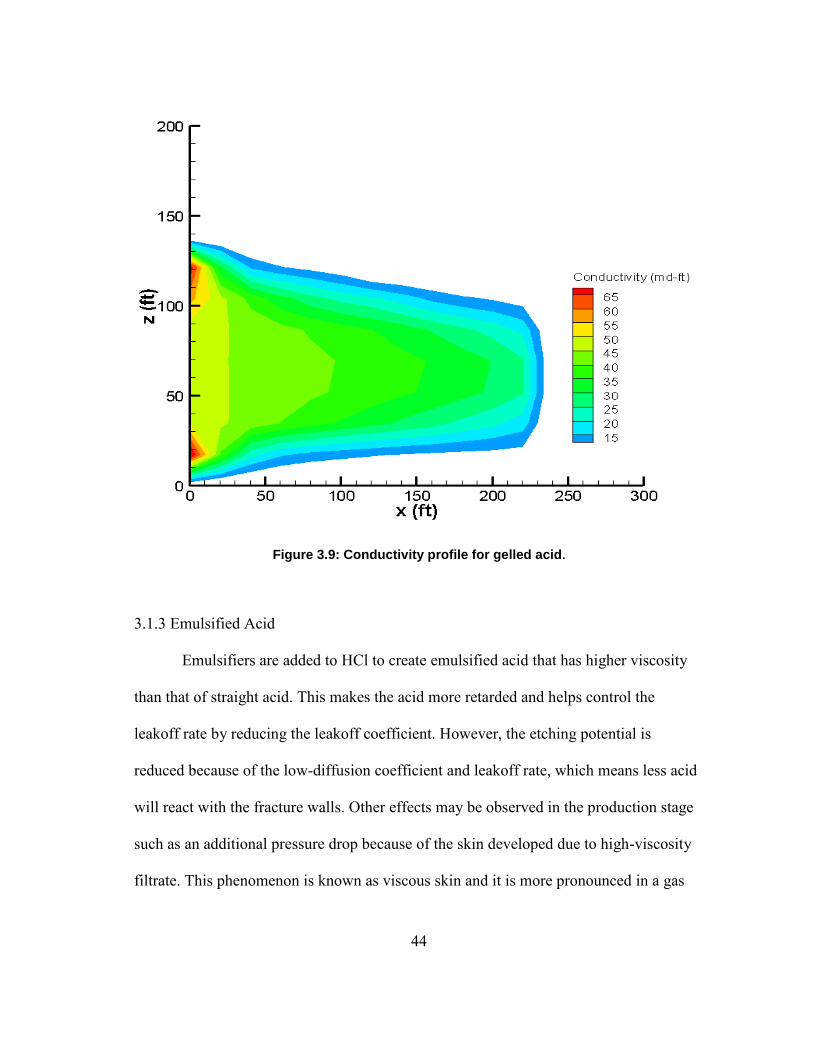
44
Figure 3.9: Conductivity profile for gelled acid.
3.1.3 Emulsified Acid
Emulsifiers are added to HCl to create emulsified acid that has higher viscosity
than that of straight acid. This makes the acid more retarded and helps control the
leakoff rate by reducing the leakoff coefficient. However, the etching potential is
reduced because of the low-diffusion coefficient and leakoff rate, which means less acid
will react with the fracture walls. Other effects may be observed in the production stage
such as an additional pressure drop because of the skin developed due to high-viscosity
filtrate. This phenomenon is known as viscous skin and it is more pronounced in a gas

45
reservoir. Simulating emulsified acid shows that acid can reach up to the tip of the
fracture (320 ft) as shown in Figure 3.10.
Figure 3.10: Velocity profile (vx) in x-direction for emulsified acid.

46
Figure 3.11: Conductivity profile for gelled acid.
The conductivity profile shows an enhanced homogenous conductivity
distribution when compared with straight or gelled acids (Fig. 3.11). This effect is
evident in acids with low-diffusion coefficients. It is observed that emulsified acid can
reach lengthy distances inside of fractures, which makes it a good candidate for very
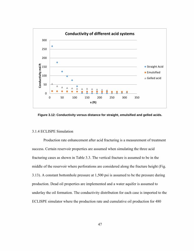
long fractures. Figure 3.12 shows conductivity along the fracture length for the three
acid systems. The straight acid has a very high conductivity at the fracture entrance, but
it drops to zero very quickly. Gelled acid has lower conductivity than straight acid but it
penetrates deeper into the fracture. Emulsified acid has the lowest conductivity but has
the greatest penetration. To measure the effect of these three treatments on the
production, files are imported into the ECLIPSE reservoir simulator.
47
Figure 3.12: Conductivity versus distance for straight, emulsified and gelled acids.
3.1.4 ECLISPE Simulation
Production rate enhancement after acid fracturing is a measurement of treatment
success. Certain reservoir properties are assumed when simulating the three acid
fracturing cases as shown in Table 3.3. The vertical fracture is assumed to be in the
middle of the reservoir where perforations are considered along the fracture height (Fig.
3.13). A constant bottomhole pressure at 1,500 psi is assumed to be the pressure during
production. Dead oil properties are implemented and a water aquifer is assumed to
underlay the oil formation. The conductivity distribution for each case is imported to the
ECLISPE simulator where the production rate and cumulative oil production for 480
0
50
100
150
200
250
300
0 50 100 150 200 250 300 350
Co
nd
uct
ivit
y m
d.f
t
x (ft)
Conductivity of different acid systems
Straight Acid
Emulsified
Gelled acid
48
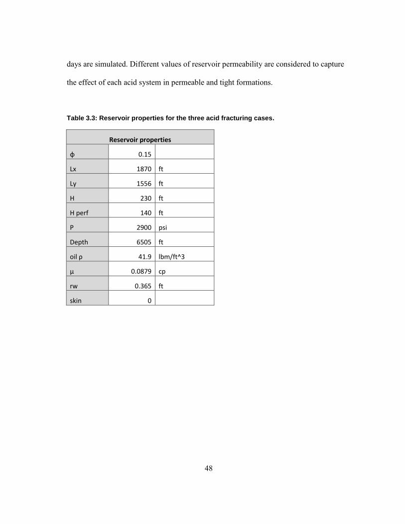
days are simulated. Different values of reservoir permeability are considered to capture
the effect of each acid system in permeable and tight formations.
Table 3.3: Reservoir properties for the three acid fracturing cases.
Reservoir properties
φ 0.15
Lx 1870 ft
Ly 1556 ft
H 230 ft
H perf 140 ft
P 2900 psi
Depth 6505 ft
oil ρ 41.9 lbm/ft^3
µ 0.0879 cp
rw 0.365 ft
skin 0
49
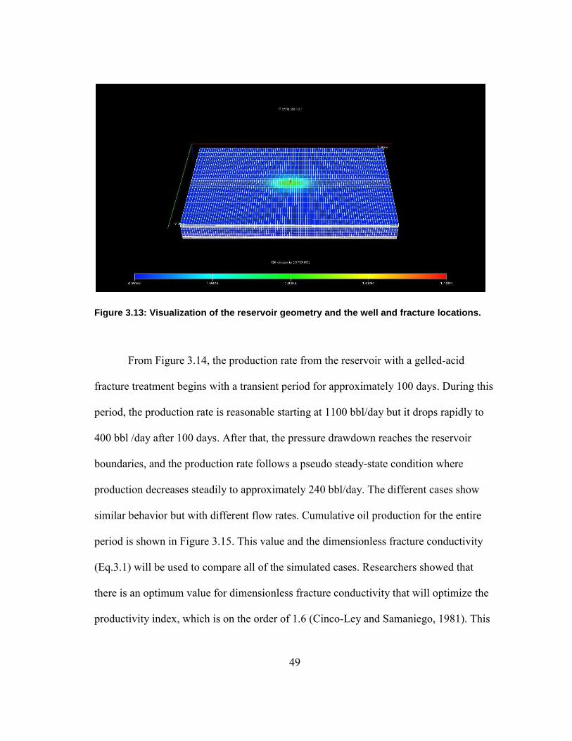
Figure 3.13: Visualization of the reservoir geometry and the well and fracture locations.
From Figure 3.14, the production rate from the reservoir with a gelled-acid
fracture treatment begins with a transient period for approximately 100 days. During this
period, the production rate is reasonable starting at 1100 bbl/day but it drops rapidly to
400 bbl /day after 100 days. After that, the pressure drawdown reaches the reservoir
boundaries, and the production rate follows a pseudo steady-state condition where
production decreases steadily to approximately 240 bbl/day. The different cases show
similar behavior but with different flow rates. Cumulative oil production for the entire
period is shown in Figure 3.15. This value and the dimensionless fracture conductivity
(Eq.3.1) will be used to compare all of the simulated cases. Researchers showed that
there is an optimum value for dimensionless fracture conductivity that will optimize the
productivity index, which is on the order of 1.6 (Cinco-Ley and Samaniego, 1981). This
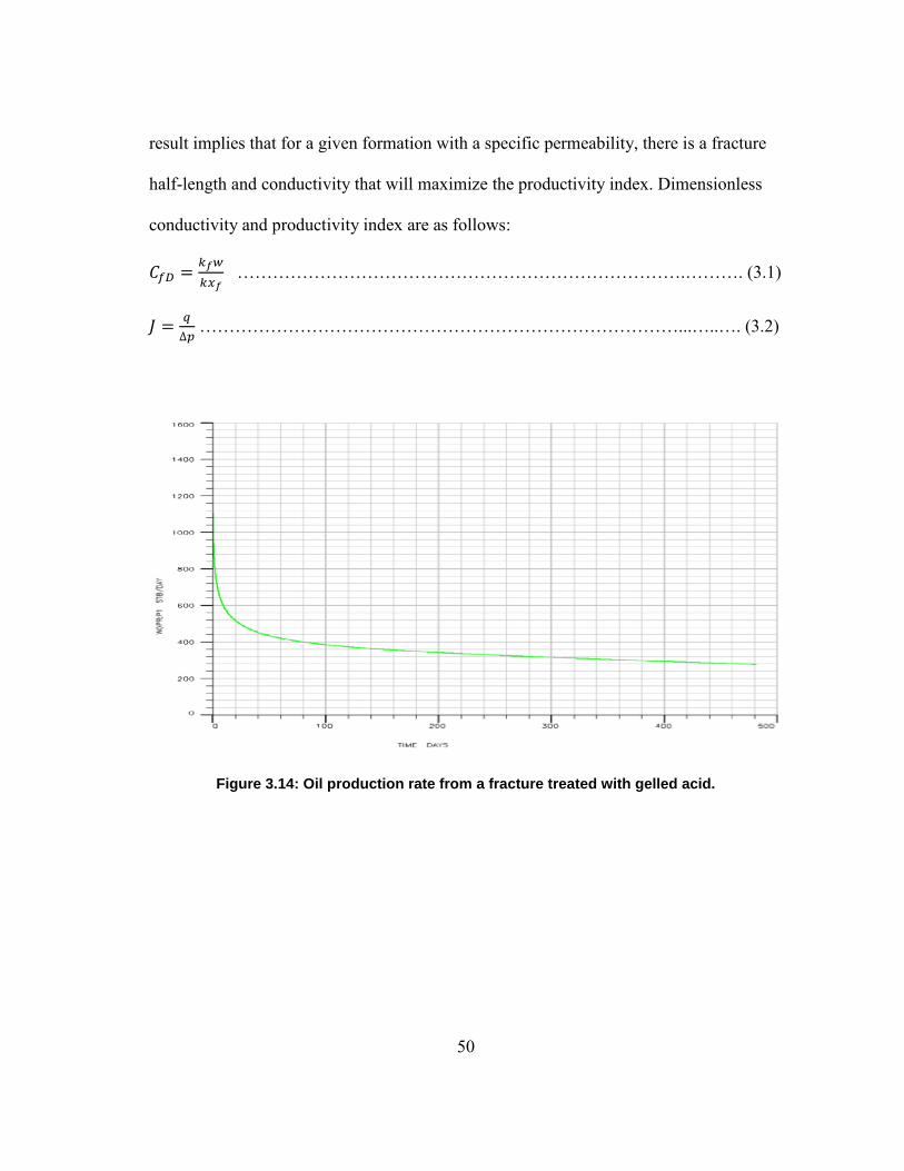
50
result implies that for a given formation with a specific permeability, there is a fracture
half-length and conductivity that will maximize the productivity index. Dimensionless
conductivity and productivity index are as follows:
………………………………………………………………….………. (3.1)
∆ ………………………………………………………………………...…..…. (3.2)
Figure 3.14: Oil production rate from a fracture treated with gelled acid.
51
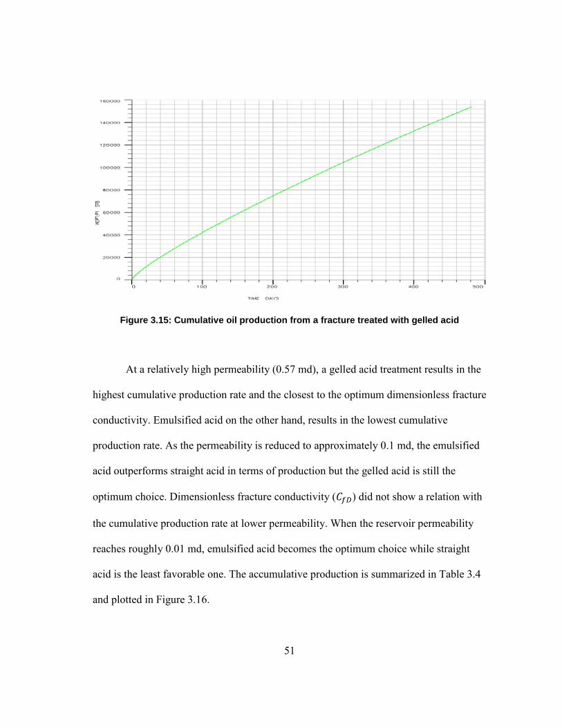
Figure 3.15: Cumulative oil production from a fracture treated with gelled acid
At a relatively high permeability (0.57 md), a gelled acid treatment results in the
highest cumulative production rate and the closest to the optimum dimensionless fracture
conductivity. Emulsified acid on the other hand, results in the lowest cumulative
production rate. As the permeability is reduced to approximately 0.1 md, the emulsified
acid outperforms straight acid in terms of production but the gelled acid is still the
optimum choice. Dimensionless fracture conductivity ( ) did not show a relation with
the cumulative production rate at lower permeability. When the reservoir permeability
reaches roughly 0.01 md, emulsified acid becomes the optimum choice while straight
acid is the least favorable one. The accumulative production is summarized in Table 3.4
and plotted in Figure 3.16.
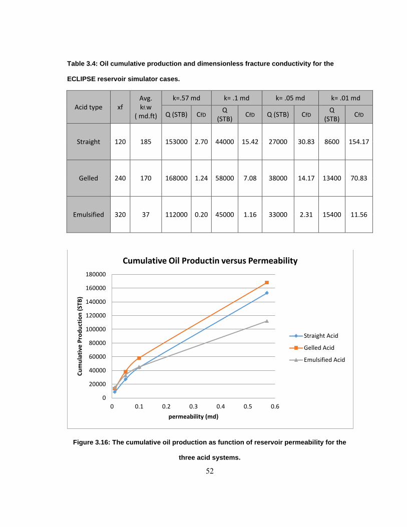
52
Table 3.4: Oil cumulative production and dimensionless fracture conductivity for the
ECLIPSE reservoir simulator cases.
Acid type xf Avg. kf.w
( md.ft)
k=.57 md k= .1 md k= .05 md k= .01 md
Q (STB) CfD Q
(STB) CfD Q (STB) CfD
Q (STB)
CfD
Straight 120 185 153000 2.70 44000 15.42 27000 30.83 8600 154.17
Gelled 240 170 168000 1.24 58000 7.08 38000 14.17 13400 70.83
Emulsified 320 37 112000 0.20 45000 1.16 33000 2.31 15400 11.56
Figure 3.16: The cumulative oil production as function of reservoir permeability for the
three acid systems.
0
20000
40000
60000
80000
100000
120000
140000
160000
180000
0 0.1 0.2 0.3 0.4 0.5 0.6
Cu
mu
lati
ve P
rod
uct
ion
(ST
B)
permeability (md)
Cumulative Oil Productin versus Permeability
Straight Acid
Gelled Acid
Emulsified Acid
53
It can be concluded that at relatively high permeability formations, creating short
and highly conductive fracture is better option than creating long and low conductivity
one. Hence, gelled acid and sometimes straight acid should be the optimum choices
since they have great etching potential but can’t reach very long distances in the fracture.
As the formation becomes tighter, the fracture will mostly act like an infinite conductive
fracture, even at low-conductivity values. This conclusion is based on the dimensionless
fracture conductivity values ( ) that are higher than 100 for the three acid systems
with roughly 0.01 md permeabilities. In this case, maximizing the acid-penetration
distance is the key factor for higher production rates that can be achieved by using an
emulsified acid or any high-viscosity fluid. In fact, increased etching volume does not
add to a production improvement in this case. This conclusion is supported by field data
from more than 70 wells in the Khuff formation within the Saudi Arabia Ghawar field.
Straight acid, emulsified acid, and in-situ gelled acid are used where emulsified acid
proved to be more suitable in low-permeability zones (Bartko et al., 2003)
3.2 Multistage Acid Injection
Acid fracturing consists of many steps where acid and pad fluids are injected in a
stage- wise procedure. The assumption of the model is that pad fluid will be injected first
and that will determine fracture height, length, and width. Then, acid is injected to etch
the wall of the fracture without changing fracture geometry. Multiple fluid systems are
used in field operations to obtain the benefit of each fluid system. Gelled acid could be
injected together with emulsified acid or crosslinked acid to achieve additional etching

54
and greater penetration distances. The simulator has the option to run more than one acid
system. In this case, an emulsified acid is injected for 20 minutes to reach the tip of
fracture followed by gelled acid for roughly 10 minutes to increase the fracture
conductivity. The result of this treatment is better than treating a fracture with 30
minutes of emulsified acid alone (Fig. 3.17). Many combinations of acid systems can be
simulated to achieve an optimum fracture conductivity and penetration distance.
Figure 3.17: Conductivity profile for emulsified acid in the left and conductivity profile for
gelled acid used as second stage in the right.
3.3 Diffusion Coefficient
Because the reaction rate is so fast, the diffusion step is the controlling step for
the reaction between HCl and the carbonate minerals. Modeling the acid diffusion lacks
diffusion coefficient data of acid systems as function of fracture width, roughness, fluid
loss rate, and Reynolds number. Therefore, the diffusion coefficient is assumed to be a

55
function of the fluid system and temperature only. This assumption causes diffusion
modeling to be inaccurate and an imprecise representative of fluid diffusion behavior in
field conditions. At a high-Peclet number, acid fracturing is fluid loss control, which
means acid spending through diffusion will have no impact on the penetration distance.
All of the cases run in the simulator have high-Peclet numbers (1 and above); hence, the
expectation is that when the diffusion coefficient is changed, penetration distance will
not be affected.
Straight acid is simulated in this case with different diffusion coefficients to
demonstrate that the fluid-loss limit will dominate the result of the treatment in this case.
All input parameters are held constant except for the diffusion coefficient. Figure 3.18
shows that penetration distance for straight acid is approximately 110 ft regardless of the
diffusion coefficient value. In terms of conductivity, a higher diffusion coefficient leads
to higher etching potential, which results in higher conductivity based on the Mou-Deng
correlation. When the Peclet number falls below 1.0, acid spending through diffusion
will control the penetration distance; however, the simulator fails to capture this
phenomena because the simulator terminates at very high diffusion values.

56
Figure 3.18: Conductivity along fracture length for different diffusion coefficient of
straight acid.
3.4 Injection Rate and Formation Type
Because the injection rate has to be equal to the leakoff rate, and because the
leakoff velocity does not change with injection rate, the leakoff distance will increase
with an increase in injection rate. The correlation between injection rate and penetration
distance is almost linear as shown in Figure 3.19. Increasing the injection rate will
increase the amount of acid reacting with the fracture walls, which results in additional
etched volume and high conductivity according to the Mou-Deng correlation. Formation
type also has an impact on the penetration distance. A dolomite formation is far less
reactive than a calcite formation; therefore, an increase in pore volume to break through
10
100
1000
10000
0 50 100 150
Co
nd
uct
ivit
y (m
d-f
t)
distance (ft)
Coductivity vs Distance for different Diffusion coefficients
De= 2.13*10^-5cm^2/sDe= 2.13*10^-6
De= 2.13*10^-7
De = 2.13*10^-4
57
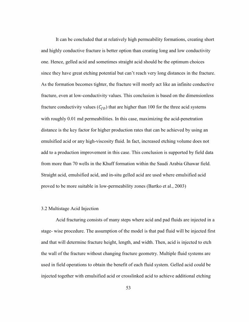
the formation is needed for dolomite ( 20) than for calcite ( = 1.5). This result
means that a dolomite formation will have a lower leakoff coefficient and therefore, acid
will be able to travel a longer distance in the fracture. This conclusion is also shown in
Figure 3.19 where a dolomite formation results in a higher penetration distance at any
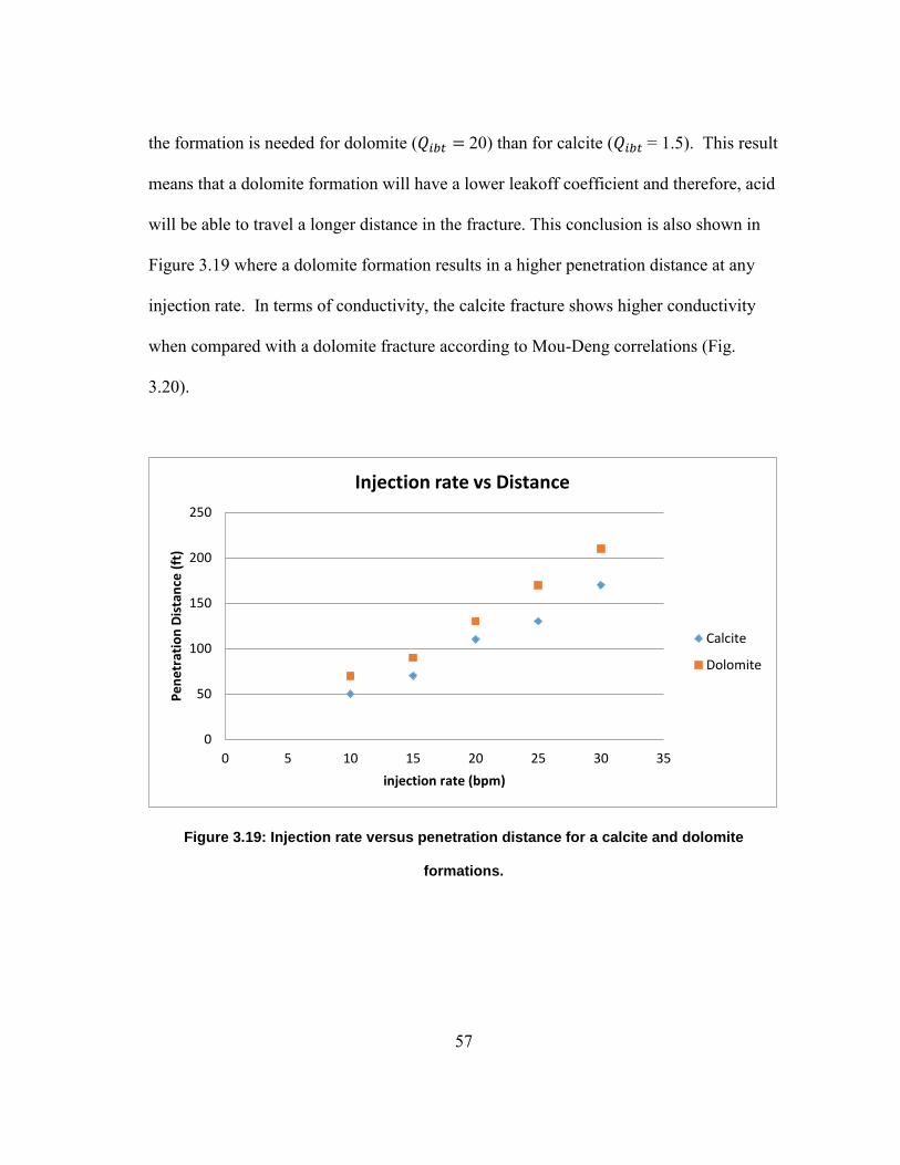
injection rate. In terms of conductivity, the calcite fracture shows higher conductivity
when compared with a dolomite fracture according to Mou-Deng correlations (Fig.
3.20).
Figure 3.19: Injection rate versus penetration distance for a calcite and dolomite
formations.
0
50
100
150
200
250
0 5 10 15 20 25 30 35
Pe
ne
trat
ion
Dis
tan
ce (
ft)
injection rate (bpm)
Injection rate vs Distance
Calcite
Dolomite
58
Figure 3.20: Conductivity versus distance for a calcite and dolomite formations.
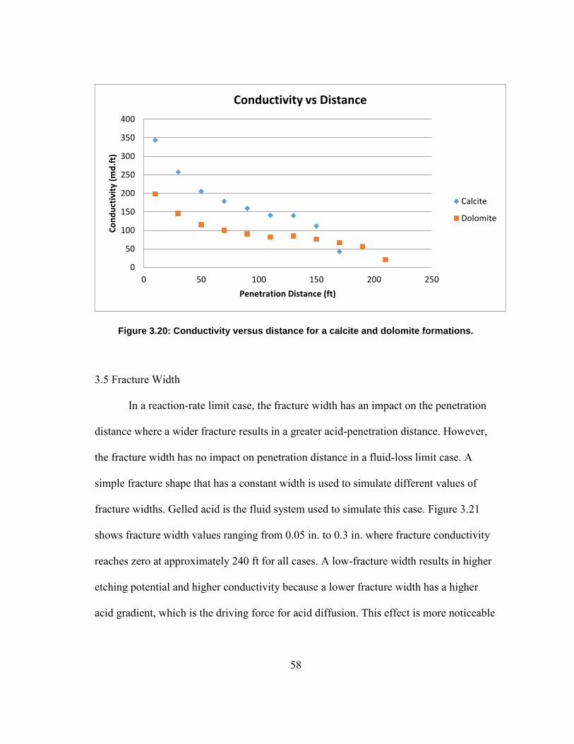
3.5 Fracture Width
In a reaction-rate limit case, the fracture width has an impact on the penetration
distance where a wider fracture results in a greater acid-penetration distance. However,
the fracture width has no impact on penetration distance in a fluid-loss limit case. A
simple fracture shape that has a constant width is used to simulate different values of
fracture widths. Gelled acid is the fluid system used to simulate this case. Figure 3.21
shows fracture width values ranging from 0.05 in. to 0.3 in. where fracture conductivity
reaches zero at approximately 240 ft for all cases. A low-fracture width results in higher
etching potential and higher conductivity because a lower fracture width has a higher
acid gradient, which is the driving force for acid diffusion. This effect is more noticeable
0
50
100
150
200
250
300
350
400
0 50 100 150 200 250
Co
nd
uct
ivit
y (m
d.f
t)
Penetration Distance (ft)
Conductivity vs Distance
Calcite
Dolomite
59
at the fracture entrance and diminishes as the acid travels deeper into the fracture. It is
necessary to mention that the conductivity is function of the acid etched width which is
different from the width created because of the hydraulic effect.
Figure 3.21: Conductivity versus distance for different values of fracture width.
3.6 Formation Permeability and Porosity
Both the effluent viscosity coefficient (Cv) and the reservoir fluid viscosity
coefficient (Cc) are linearly increasing with the square root of reservoir permeability.
Therefore, highly permeable formations result in a low-penetration distance because of
the excessive leakoff rate. This relation is shown clearly in Figure 3.22 where the
0
50
100
150
200
250
0 50 100 150 200 250 300 350
con
du
ctiv
ity
md
.ft
Distance (ft)
Conductivity vs Distance for different fracture width
w=.05 in
w=0.1 in
w=0.15 in
w= 0.2 in
w = 0.3 in
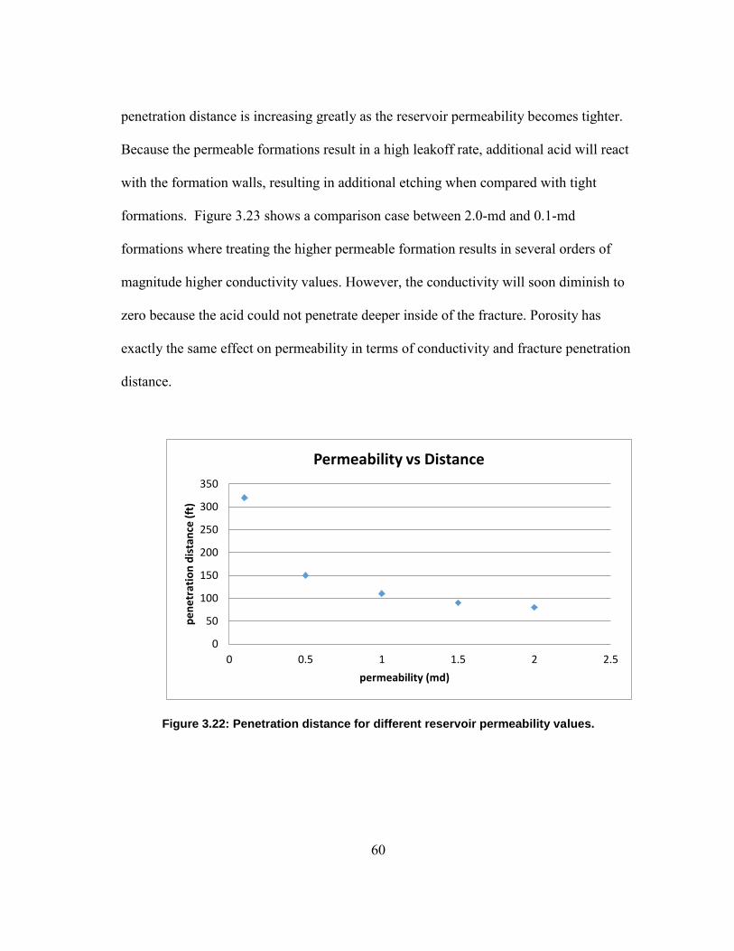
60
penetration distance is increasing greatly as the reservoir permeability becomes tighter.
Because the permeable formations result in a high leakoff rate, additional acid will react
with the formation walls, resulting in additional etching when compared with tight
formations. Figure 3.23 shows a comparison case between 2.0-md and 0.1-md
formations where treating the higher permeable formation results in several orders of
magnitude higher conductivity values. However, the conductivity will soon diminish to
zero because the acid could not penetrate deeper inside of the fracture. Porosity has
exactly the same effect on permeability in terms of conductivity and fracture penetration
distance.
Figure 3.22: Penetration distance for different reservoir permeability values.
0
50
100
150
200
250
300
350
0 0.5 1 1.5 2 2.5
pe
ne
trat
ion
dis
tan
ce (
ft)
permeability (md)
Permeability vs Distance
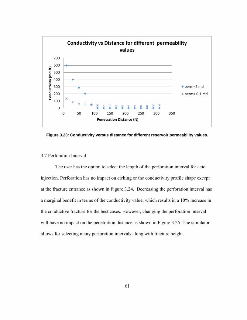
61
Figure 3.23: Conductivity versus distance for different reservoir permeability values.
3.7 Perforation Interval
The user has the option to select the length of the perforation interval for acid
injection. Perforation has no impact on etching or the conductivity profile shape except
at the fracture entrance as shown in Figure 3.24. Decreasing the perforation interval has
a marginal benefit in terms of the conductivity value, which results in a 10% increase in
the conductive fracture for the best cases. However, changing the perforation interval
will have no impact on the penetration distance as shown in Figure 3.25. The simulator
allows for selecting many perforation intervals along with fracture height.
0
100
200
300
400
500
600
700
0 50 100 150 200 250 300 350
Co
nd
uct
ivit
y (m
d.f
t)
Penetration Distance (ft)
Conductivity vs Distance for different permeability values
perm=2 md
perm= 0.1 md

62
Figure3.24: Conductivity profile for emulsified acid that has 40 ft perforation interval at
the fracture entrance.
Figure 3.25: Conductivity vs distance for different perforation intervals.
0
2
4
6
8
10
12
14
16
0 50 100 150 200 250 300 350
con
du
ctiv
ity
md
.ft
Penetration Distance (ft)
Different perforations interval
total interval
perf (40 ft)
perf (20 ft)
perf (60 ft)

63
CHAPTER IV
MODEL LIMITATIONS
4.1 Limitations Due to Model Assumptions
To solve the governing equations in this model, many assumptions are
considered (discussed in Chapter 2). These assumptions can be a source of imprecision,
but in such a stochastic process, these errors can be negligible when compared with
errors caused by formation heterogeneity. The ability to quantify the amount of
inaccuracy due to these assumptions will enable us to validate or reject these
assumptions.
When acid reacts with the fracture wall, the heat from the reaction is released and
transferred by convection due to fluid movement and conduction through the fracture
walls. Temperature will continuously change during acid injection because this
phenomenon has an impact on the rate of acid reaction and the amount of rock dissolved.
To account for these effects, energy balance equations and the heat transfer equation
should be considered, both of which will add complexity to the model. This model does
not account for heat transfer and assumes an isothermal temperature.
Gravity has an impact on the fluid flow behavior that may add complexity to the
flow in the fracture height direction. Also, gravity will allow the fluid to concentrate
more in the bottom of the fracture. This condition will affect the acid etching profile;
hence, the conductivity profile inside of the fracture. Many fracturing models do not

64
account for gravity and assume that it has negligible effect. This model excludes
gravity, assuming the effect will be insignificant.
The model can simulate multistage processes of different acid systems but does
not couple it with the mechanical behavior of the fracture. All pad fluid is assumed to be
pumped as one stage to create a fixed fracture geometry that will not change during acid
injection. Fracture geometry is imported from other commercial simulators; however,
only acid injection will be simulated in our simulator. In field cases, acid and pad fluids
are injected in a stage-wise process, which means acid injection will impact fracture
geometry. Failure to couple acid injection with the geometry model can result in
significant error and is considered the major limitation of the model. In the coupled case,
fracture length, width, and height will keep changing during most of the stages.
The reservoir is assumed to be layered, which means the simulator will allow for
entering properties of each layer instead of properties of each grid block; thus, the user
has to specify each layer permeability and mineralogy. This procedure is valid for short
fractures, but could be an invalid assumption for very long fractures.
65
4.2 Limitations Due to Numerical Errors
The SIMPLE algorithm is used to solve the Navier- Stokes equations. The
consistency index (k) and the power low exponent (n) values have a large impact on the
solution stability of the simulator. Some values will result in numerical errors that cause
the simulator to terminate without completing the run. Pressure inside of the fracture
should be maintained at an almost constant value during injection time; however, an
unstable solution makes the pressure drop quickly at each time step until the pressure
reaches zero, and hence, the simulation terminates. A high-diffusion coefficient also can
cause a decrease of pressure inside of the fracture to zero, which imposes an upper limit
on the diffusion coefficient value. Changing the number of grid blocks or the size of
each grid block causes the solution to terminate if not changed proportionally. These
numerical errors place a limit on the various simulation cases that can be run in this
simulator.
For the PKN geometry model, the width of the fracture is assumed to decrease
gradually until reaching the tip of the fracture. The geometry used in most of the cases
shows a sharp decrease in fracture height at the middle of the fracture. As Figure 4.1
shows, conductivity suddenly increased at that location because the fluid has to converge
to the smaller fracture opening.
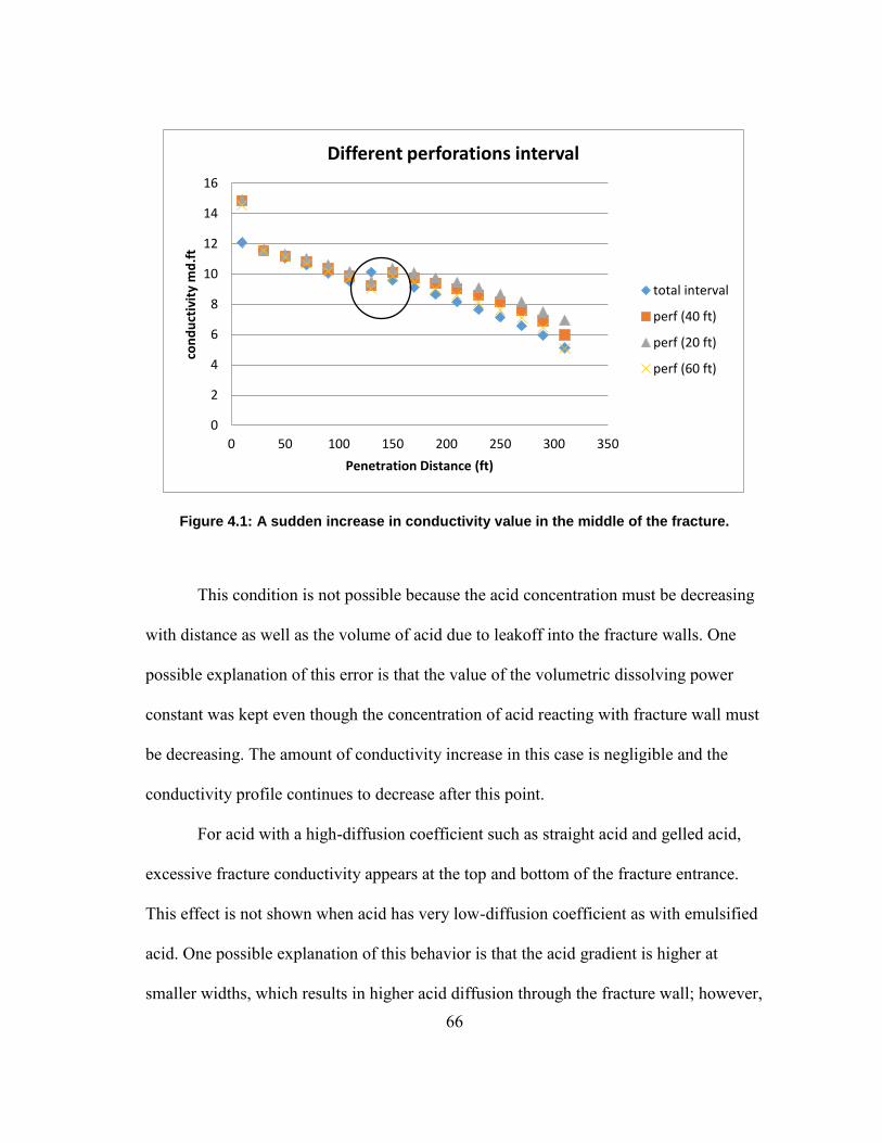
66
Figure 4.1: A sudden increase in conductivity value in the middle of the fracture.
This condition is not possible because the acid concentration must be decreasing
with distance as well as the volume of acid due to leakoff into the fracture walls. One
possible explanation of this error is that the value of the volumetric dissolving power
constant was kept even though the concentration of acid reacting with fracture wall must
be decreasing. The amount of conductivity increase in this case is negligible and the
conductivity profile continues to decrease after this point.
For acid with a high-diffusion coefficient such as straight acid and gelled acid,
excessive fracture conductivity appears at the top and bottom of the fracture entrance.
This effect is not shown when acid has very low-diffusion coefficient as with emulsified
acid. One possible explanation of this behavior is that the acid gradient is higher at
smaller widths, which results in higher acid diffusion through the fracture wall; however,
0
2
4
6
8
10
12
14
16
0 50 100 150 200 250 300 350
con
du
ctiv
ity
md
.ft
Penetration Distance (ft)
Different perforations interval
total interval
perf (40 ft)
perf (20 ft)
perf (60 ft)
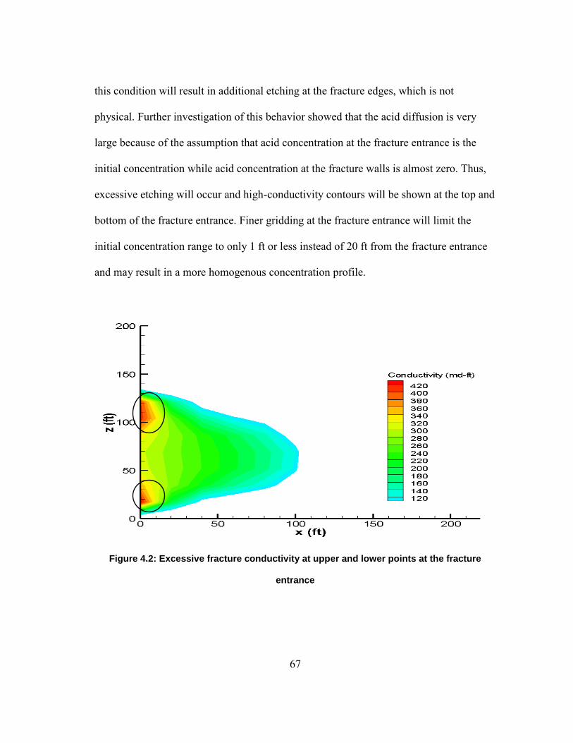
67
this condition will result in additional etching at the fracture edges, which is not
physical. Further investigation of this behavior showed that the acid diffusion is very
large because of the assumption that acid concentration at the fracture entrance is the
initial concentration while acid concentration at the fracture walls is almost zero. Thus,
excessive etching will occur and high-conductivity contours will be shown at the top and
bottom of the fracture entrance. Finer gridding at the fracture entrance will limit the
initial concentration range to only 1 ft or less instead of 20 ft from the fracture entrance
and may result in a more homogenous concentration profile.
Figure 4.2: Excessive fracture conductivity at upper and lower points at the fracture
entrance
68
CHAPTER V
CONCLUSION AND RECOMMENDATIONS
5.1 Conclusion
Acid fracturing is a well stimulation technique used in carbonate reservoirs.
Developing a theortical model can help to optimize the treatment parameters for acid
fracturing. The model developed uses other commercial software to import the initial
fracture geometry. The Navier-Stokes (momentum balance) and continuity (mass
balance) equations are solved for pressure and velocity profiles. Once the velocity
profile is computed, the acid balance equation can be solved for the acid concentration
profile. Obtaining a concentration profile helps in calculating the amount of rock etched
through diffusion and convection (leaking through fracture walls). Conductivity
distribution is calculated using the Deng-Mou correlation where statistical parameters
are used to account for fracture heterogeneity. This conductivity distribution can be
imported to other reservoir simulators such as the ECLIPSE simulator to compute the
production rate after completing the treatment.
Two important parameters will determine a production increase from a fractured
well; these are fracture conductivity and acid penetration distance. Straight acid, gelled
acid, and emulsified acid are simulated to observe the effect of these fluids on the two
parameters. Straight acid shows strong etching potential, resulting in high conductivity
but it leaks off completely near the fracture entrance. Gelled acid has a medium etching
strength and can reach greater distances than with straight acid. Emulsified acid has the
69
lowest etching potential, resulting in the lowest conductivity but it reaches greater
distances than the other acid systems. Conductivity distributions along the fracture are
imported into the ECLIPSE Simulator to simulate production rates for each case. In
high-permeability formations, gelled acid results in the highest production rate because
high conductivity is more favorable than low conductivity and a long penetration
distance. In low-permeability formations, emulsified acid yields the best results because
the acid penetration distance is more favorable in this case than creating short and high-
conductivity fractures. A combination of the different acid systems can result in the
optimum production case where the simulator allows for using more than one stage of an
acid system.
The fluid loss limit case is assumed in this simulator, which means nothing will
alter the acid penetration distance except for the parameters that affect the leakoff
coefficient. Hence, the diffusion coefficient will have no impact on the acid penetration
distance but it will affect the fracture conductivity value. A higher injection rate will
result in a greater penetration distance and increased conductivity because a higher
volume of acid is pumped. Acid tends to travel a greater distance in fractures in dolomite
than in calcite. The reason for this result is that dolomite is far more resistible to
wormholing than is calcite. Nevertheless, acid will create more etching in calcite,
resulting in better conductivity when assuming the Deng-Mou correlation. The fracture
width impacts the penetration distance in the reaction rate limit case where a wider
fracture will allow fluid to travel a greater distance in the fracture. However, in the fluid
loss limit case, the fracture width will not affect the acid penetration distance but it will
70
have an impact on the conductivity value where a lower width gives better conductivity.
Formation permeability and porosity will have similar effects. A more porous and
permeable formation usually results in a lower penetration distance because of higher
leakoff rate. On the other hand, more etching will result from acid leaking through the
fracture wall. A simulator allows the user to specify the perforation interval, where a
smaller perforation range results in a marginal increase in the average conductivity
value; however, changing the length of perforation interval will not have any impact on
the penetration distance.
5.2 Recommendations
Coupling an acid fracturing model with a geomechanical model to simulate
fracture propagation as fluid is injected should be considered. This model will allow for
making more accurate fracture geometry predictions in terms of height, length, and
width. Also, including a heat transfer model makes the fracture model more powerful
because temperature has a strong impact on the reaction rate between an acid and
carbonate minerals. Including a temperature profile makes the simulator more
representatives of filed applications. However, before including heat transfer and
geomechanical models, numerical errors resulting from Navier-Stokes equations should
be solved to make the simulator more stable. Changing fracture geometry or other
treatment parameters can result in a rapid decrease in pressure inside of the fracture,

71
which causes the simulator to stop early in the process. Solving this problem is the first
priority before coupling the model.

72
REFERENCES
Bartko, K.M., Nasr-El-Din, H.A., Rahim, Z., and Al-Muntasheri, G.A. 2003. Acid
Fracturing of a Gas Carbonate Reservoir: The Impact of Acid Type and Lithology on
Fracture Half Length and Width. Paper SPE 84130 presented at the SPE Annual
Technical Conference and Exhibition, Denver, Colorado, 5-8 October.
Ben-Naceur, K. and Economides, M.J. 1989. Design and Evaluation of Acid Fracturing
Treatments. Paper SPE 18978 presented at the SPE Joint Rocky Mountain Regional/Low
Permeability Reservoirs Symposium and Exhibition, Denver, Colorado, 6-8 March.
Crowe, C.W., Martin, R.C., and Michaelis, A.M. 1981. Evaluation of Acid-Gelling
Agents for Use in Well Stimulation. SPEJ 21(2): 415-424.
De Rozieres, J. 1994. Measuring Diffusion Coefficients in Acid Fracturing Fluids and
Their Application to Gelled and Emulsified Acids. Paper SPE 28552 presented at the
SPE Annual Technical Conference and Exhibition, New Orleans, Louisiana, 25-28
September.
Deng, J., Mou, J., Hill, A.D., and Zhu, D. 2012. A New Correlation of Acid-Fracture
Conductivity Subject to Closure Stress. SPE Prod. & Oper. 27(2): 158-169.
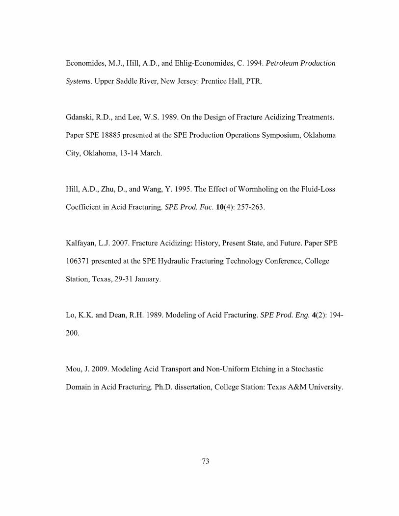
73
Economides, M.J., Hill, A.D., and Ehlig-Economides, C. 1994. Petroleum Production
Systems. Upper Saddle River, New Jersey: Prentice Hall, PTR.
Gdanski, R.D., and Lee, W.S. 1989. On the Design of Fracture Acidizing Treatments.
Paper SPE 18885 presented at the SPE Production Operations Symposium, Oklahoma
City, Oklahoma, 13-14 March.
Hill, A.D., Zhu, D., and Wang, Y. 1995. The Effect of Wormholing on the Fluid-Loss
Coefficient in Acid Fracturing. SPE Prod. Fac. 10(4): 257-263.
Kalfayan, L.J. 2007. Fracture Acidizing: History, Present State, and Future. Paper SPE
106371 presented at the SPE Hydraulic Fracturing Technology Conference, College
Station, Texas, 29-31 January.
Lo, K.K. and Dean, R.H. 1989. Modeling of Acid Fracturing. SPE Prod. Eng. 4(2): 194-
200.
Mou, J. 2009. Modeling Acid Transport and Non-Uniform Etching in a Stochastic
Domain in Acid Fracturing. Ph.D. dissertation, College Station: Texas A&M University.

74
Mou, J., Zhu, D., and Hill, A.D. 2010. Acid-Etched Channels in Heterogeneous
Carbonates–A Newly Discovered Mechanism for Creating Acid-Fracture Conductivity.
SPEJ 15(2): 404-416.
Nierode, D.E., Williams, B.R., and Bombardieri, C.C. 1972. Prediction of Stimulation
from Acid Fracturing Treatments. JCPT 11(4): 31-41
Nierode, D.E. and Kruk, K.F. 1973. An Evaluation of Acid Fluid Loss Additives,
Retarded Acids, and Acidized Fracture Conductivity. Paper SPE 4549 presented at the
SPE Annual Fall Meeting, Las Vegas, Nevada, 30 September – 3 October.
Nierode, D.E. and Williams, B.B. 1971. Characteristics of Acid Reaction in Limestone
Formations. SPEJ 11(4): 406-418.
Nieto, C.M., Pournik, M., and Hill, A.D. 2008. The Texture of Acidized Fracture
Surfaces: Implications for Acid Fracture Conductivity. SPE Prod. & Oper. 23(3): 343-
352.
Oeth, C. 2013. Three Dimensional Modeling of Acid Transport and Etching in a
Fracture. Ph.D. dissertation, College Station: Texas A&M University.

75
Oeth, C.V., Hill, A.D., and Zhu, D. 2014. Acid Fracture Treatment Design with Three-
Dimensional Simulation. Paper SPE 168602 presented at the SPE Hydraulic Fracturing
Technology Conference, The Woodlands, Texas, 4-6 February.
Penny, G.S. and Conway, M.W. 1989. Chapter 8, Fluid Leakoff. In Recent Advances in
Hydraulic Fracturing, eds. J.L. Gidley, S.A. Holditch, D.E. Nierode, and R.W. Veatch,
Jr., 388-393. Richardson, Texas: Society of Petroleum Engineers.
Schechter, Robert S. 1992. Oil Well Stimulation. Englewood Cliffs, New Jersey:
Prentice-Hall, Inc.
Settari, A. 1993. Modeling of Acid-Fracturing Treatments. SPE Prod. & Fac. 8(1): 30-
38.
Settari, A., Sullivan, R.B., and Hansen, C. 2001. A New Two-Dimensional Model for
Acid-Fracturing Design. SPE Prod. & Fac. 16(4): 200-209.
Williams, B.B. and Nierode, D.E. 1972. Design of Acid Fracturing Treatments. JPT
24(7): 849-859.
Williams, B.B., Gidley, J.L., and Schechter, R.S. 1979. Acidizing Fundamentals. Dallas,
Texas: Society of Petroleum Engineers of AIME.
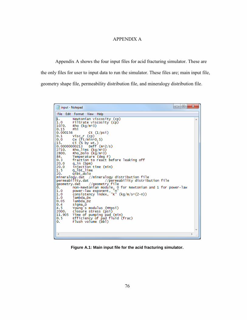
76
APPENDIX A
Appendix A shows the four input files for acid fracturing simulator. These are
the only files for user to input data to run the simulator. These files are; main input file,
geometry shape file, permeability distribution file, and mineralogy distribution file.
Figure A.1: Main input file for the acid fracturing simulator.
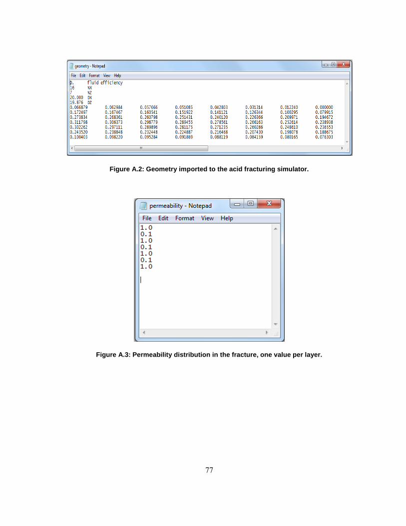
77
Figure A.2: Geometry imported to the acid fracturing simulator.
Figure A.3: Permeability distribution in the fracture, one value per layer.
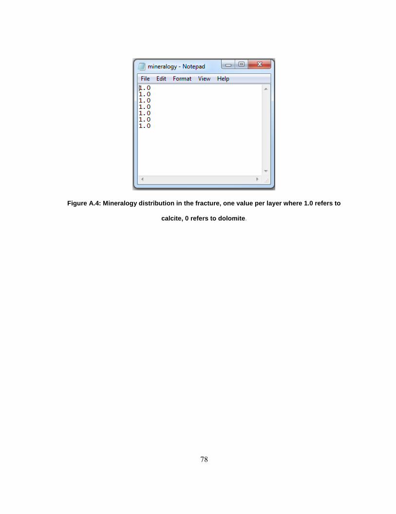
78
Figure A.4: Mineralogy distribution in the fracture, one value per layer where 1.0 refers to
calcite, 0 refers to dolomite.

79
APPENDIX B
Appendix B shows the three input files for the ECLIPSE reservoir simulator. The
main input file is to create the reservoir and fluid properties and to specify the gridding
pattern for the reservoir. The well specification file is used to specify the perforation
interval for production, well location and the production mode of the well (constant rate
or constant pressure). The permeability distribution file is used to specify the
permeability of the reservoir and the fracture after converting conductivity into
permeability assuming constant fracture width of 0.1 inch.
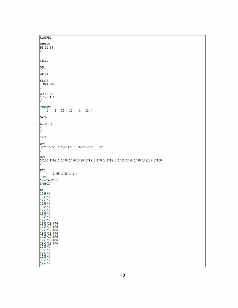
80
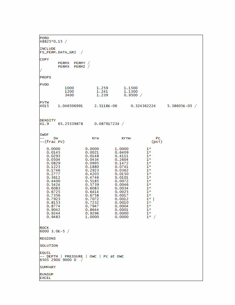
81
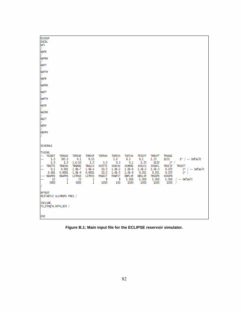
82
Figure B.1: Main input file for the ECLIPSE reservoir simulator.
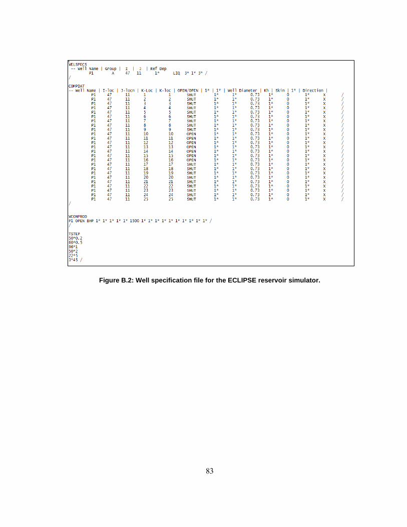
83
Figure B.2: Well specification file for the ECLIPSE reservoir simulator.
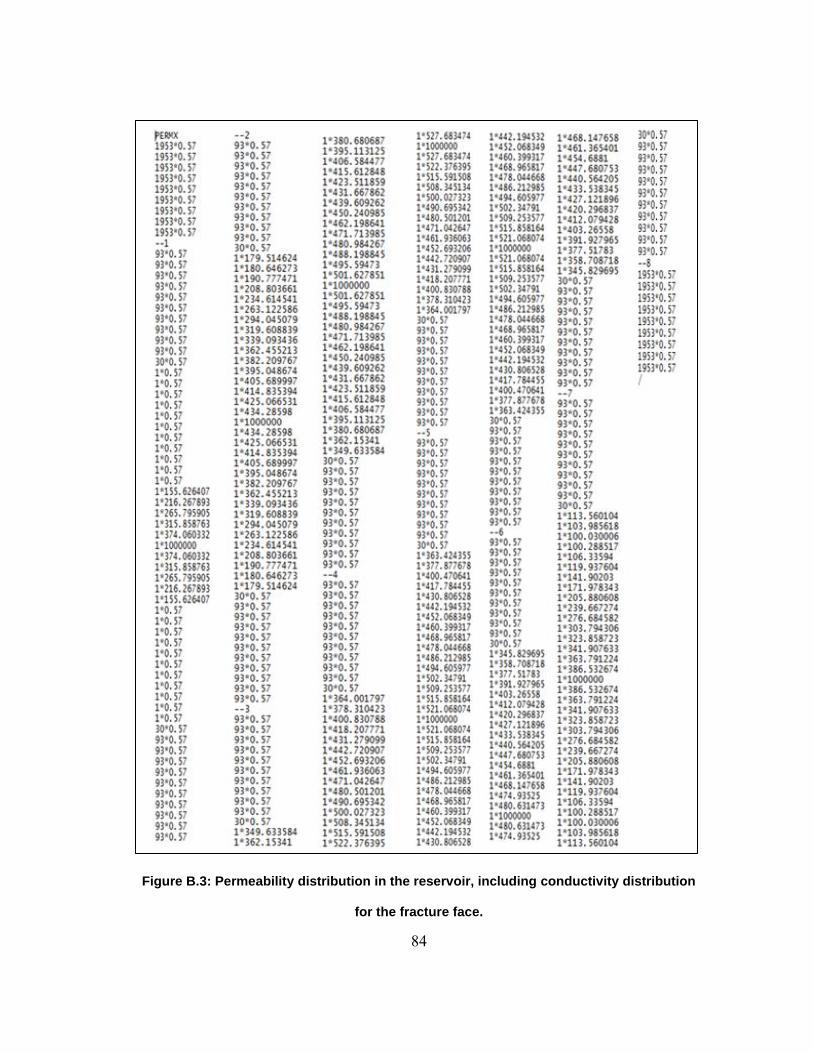
84
Figure B.3: Permeability distribution in the reservoir, including conductivity distribution
for the fracture face.
Related Documents