Welcome message from author
This document is posted to help you gain knowledge. Please leave a comment to let me know what you think about it! Share it to your friends and learn new things together.
Transcript
modeling multiphase flow in heterogeneous
media using streamtubes
a dissertation
submitted to the department of petroleum engineering
and the committee on graduate studies
of stanford university
in partial fulfillment of the requirements
for the degree of
doctor of philosophy
By
Marco Roberto Thiele
December 1994
Nothing enters the mind more readily than geometric �gures.
Descartes, 1596{1650
Dedicated with love to
Nicola and Valentina.
c Copyright by Marco Roberto Thiele 1994
All Rights Reserved
ii
I certify that I have read this dissertation and that in my opinion
it is fully adequate, in scope and quality, as a dissertation for the
degree of Doctor of Philosophy.
Dr. Franklin M. Orr (Principal Adviser)
I certify that I have read this dissertation and that in my opinion
it is fully adequate, in scope and quality, as a dissertation for the
degree of Doctor of Philosophy.
Dr. Martin Blunt (co-Adviser)
I certify that I have read this dissertation and that in my opinion
it is fully adequate, in scope and quality, as a dissertation for the
degree of Doctor of Philosophy.
Dr. Thomas A. Hewett
I certify that I have read this dissertation and that in my opinion
it is fully adequate, in scope and quality, as a dissertation for the
degree of Doctor of Philosophy.
Dr. Khalid Aziz
Approved for the University Committee on Graduate Studies:
iii
Abstract
Streamtubes are used to determine fast and accurate solutions to multiphase, multi-
component displacements through heterogeneous, cross-sectional systems. Solutions
are constructed by treating each streamtube as a one-dimensional system along which
mass conservations equations are solved, either analytically or numerically. The non-
linearity of the underlying ow �eld is resolved by periodically updating the stream-
tubes and remapping the one-dimensional solution(s) as an integration from tD = 0
to tD = tD + �tD. Examples for (1) tracer ow, (2) two-phase immiscible ow, (3)
�rst contact miscible ow, and (4) two-phase, compositional ow demonstrate that
recoveries and large-scale displacements characteristics dictated by reservoir hetero-
geneity can be predicted accurately using two to �ve orders of magnitude less com-
putation time than traditional simulation approaches. Mapping analytical solutions
along streamtubes allows di�usion-free, two-dimensional solutions to be found. By
comparing streamtube solutions to traditional �nite di�erence solutions, numerical
di�usion is shown to reduce substantially and in some cases even to eliminate com-
pletely the mobility contrast in compositional displacements. The coupling of phase
behavior and numerical di�usion is found to be so dominant as to force only very
slow convergence of the solution by progressive grid re�nement. The speed of the
streamtube method is used to quantify the uncertainty in recovery arising from the
statistical description of reservoir heterogeneity interacting with the inherent nonlin-
earity of the problem formulation. The uncertainty is shown to be signi�cant and
characterized by a large spread in overall recovery.
iv
Acknowledgments
My years at Stanford as a PhD student have been wonderful ones. I owe this to many
people who, in their own way, have helped me complete this work successfully and
have made my stay on the Farm so rewarding.
I am deeply indebted to my supervisor, Lynn Orr, for taking me into his research
group and for supporting me all these years. I am grateful for the freedom he has
allowed me in exploring the vast academic resources available at Stanford and for the
opportunity to teach PE251 { Thermodynamics of Phase Equilibria. My co-advisor,
Martin Blunt, has been a source of enthusiasm and support for this work, and his
untiring push and criticism were determining factors in shaping this dissertation. I
thank Tom Hewett and Khalid Aziz for their careful reading and constructive sug-
gestions. I must acknowledge Roland Horne for his incredible stamina in computer
matters, which has aided this research signi�cantly, and Christina and Yolanda for
helping me �nd my way through Stanford's administrative maze. John and Rafael
have been a formidable duo to share an o�ce with, and Chick's GPS program has
been invaluable for presenting my work. An encompassing thank you to all who have
contributed in making the department such an enjoyable and productive environment
to work in. The �nancial support of all SUPRI-C a�liates and DOE is also gratefully
acknowledged.
I thank the Bourke family for a memorable �rst year and warm embrace, and
Paula and Phillip Kirkeby for their sincere friendship. Although far away, the loving
support of my parents, Maria-Gloria and Roberto, my sister, Alessandra, and my
grandmother, Valentina, could not have been felt closer. Finally, I thank Nicola
for riding with me on the inevitable rollercoaster of euphoria and depression that is
inherent in getting a PhD, and paralleled in life and love.
v
Contents
Abstract iv
Acknowledgments v
1 Introduction 1
1.1 Streamtubes and The Riemann Approach : : : : : : : : : : : : : : : : 2
1.2 Nonlinearity : : : : : : : : : : : : : : : : : : : : : : : : : : : : : : : : 3
1.3 Class of Problems : : : : : : : : : : : : : : : : : : : : : : : : : : : : : 3
1.4 Outline : : : : : : : : : : : : : : : : : : : : : : : : : : : : : : : : : : : 4
2 Literature Review 7
2.1 Introduction : : : : : : : : : : : : : : : : : : : : : : : : : : : : : : : : 7
2.2 Petroleum Literature : : : : : : : : : : : : : : : : : : : : : : : : : : : 8
2.3 Groundwater Literature : : : : : : : : : : : : : : : : : : : : : : : : : 14
2.4 Boundary Element Methods : : : : : : : : : : : : : : : : : : : : : : : 15
2.5 Front Tracking : : : : : : : : : : : : : : : : : : : : : : : : : : : : : : 17
2.6 Concluding Remarks : : : : : : : : : : : : : : : : : : : : : : : : : : : 17
3 Mathematical Model 19
3.1 Introduction : : : : : : : : : : : : : : : : : : : : : : : : : : : : : : : : 19
3.2 The Streamfunction - Constant Coe�cients : : : : : : : : : : : : : : 20
3.3 The Streamfunction - Variable Coe�cients : : : : : : : : : : : : : : : 22
3.4 Boundary Conditions : : : : : : : : : : : : : : : : : : : : : : : : : : : 24
3.5 Numerical Solution : : : : : : : : : : : : : : : : : : : : : : : : : : : : 26
vi
3.6 Streamtubes : : : : : : : : : : : : : : : : : : : : : : : : : : : : : : : : 27
3.7 Streamtubes as 1D Systems : : : : : : : : : : : : : : : : : : : : : : : 30
3.7.1 Mapping of a 1D Solution - Method A : : : : : : : : : : : : : 32
3.7.2 Mapping of a 1D Solution - Method B : : : : : : : : : : : : : 33
3.7.3 Mapping 1D Solutions Onto a 2D Cartesian Grid : : : : : : : 34
4 Unit Mobility Displacements 36
4.1 Introduction : : : : : : : : : : : : : : : : : : : : : : : : : : : : : : : : 36
4.2 Streamtubes : : : : : : : : : : : : : : : : : : : : : : : : : : : : : : : : 37
4.3 2D Displacements - No Physical Di�usion : : : : : : : : : : : : : : : 39
4.3.1 The 1D Solution : : : : : : : : : : : : : : : : : : : : : : : : : 39
4.3.2 The 2D Solution : : : : : : : : : : : : : : : : : : : : : : : : : 42
4.3.3 Sensitivity of 2D Solution : : : : : : : : : : : : : : : : : : : : 44
4.4 2D Displacements - Physical Di�usion : : : : : : : : : : : : : : : : : 46
4.4.1 The 1D Solution : : : : : : : : : : : : : : : : : : : : : : : : : 46
4.4.2 The 2D Solution : : : : : : : : : : : : : : : : : : : : : : : : : 48
4.5 Quantifying Numerical Di�usion : : : : : : : : : : : : : : : : : : : : : 53
4.6 Concluding Remarks : : : : : : : : : : : : : : : : : : : : : : : : : : : 53
5 Immiscible Displacements 56
5.1 Introduction : : : : : : : : : : : : : : : : : : : : : : : : : : : : : : : : 56
5.1.1 The Riemann Approach : : : : : : : : : : : : : : : : : : : : : 57
5.1.2 Reasons for the Riemann Approach : : : : : : : : : : : : : : : 58
5.2 The 1D Buckley{Leverett Solution : : : : : : : : : : : : : : : : : : : 59
5.3 Validation of the Riemann Approach : : : : : : : : : : : : : : : : : : 60
5.4 Convergence of the Riemann Approach : : : : : : : : : : : : : : : : : 65
5.5 Other Immiscible Solutions : : : : : : : : : : : : : : : : : : : : : : : : 66
5.5.1 End-Point Mobility Ratio : : : : : : : : : : : : : : : : : : : : 66
5.5.2 Reservoir Heterogeneity : : : : : : : : : : : : : : : : : : : : : 67
5.6 The Higgins and Leighton Method : : : : : : : : : : : : : : : : : : : 80
5.7 Concluding Remarks : : : : : : : : : : : : : : : : : : : : : : : : : : : 83
vii
6 First-Contact Miscible Displacements 84
6.1 Introduction : : : : : : : : : : : : : : : : : : : : : : : : : : : : : : : : 84
6.2 The Assumptions in FCM Flow : : : : : : : : : : : : : : : : : : : : : 85
6.3 The One-Dimensional Solution(s) : : : : : : : : : : : : : : : : : : : : 87
6.3.1 Scale of 1D Solutions : : : : : : : : : : : : : : : : : : : : : : : 89
6.4 2D Solutions With No Di�usion : : : : : : : : : : : : : : : : : : : : : 91
6.5 2D Solutions Using the CD-Equation : : : : : : : : : : : : : : : : : : 98
6.6 2D Solutions Using Viscous Fingering Model : : : : : : : : : : : : : : 108
6.7 Convergence : : : : : : : : : : : : : : : : : : : : : : : : : : : : : : : : 119
6.7.1 The Higgins and Leighton Approach : : : : : : : : : : : : : : 122
6.8 Applications : : : : : : : : : : : : : : : : : : : : : : : : : : : : : : : : 125
6.9 Concluding Remarks : : : : : : : : : : : : : : : : : : : : : : : : : : : 127
7 Compositional Displacements 130
7.1 Introduction : : : : : : : : : : : : : : : : : : : : : : : : : : : : : : : : 130
7.2 One-Dimensional Solutions : : : : : : : : : : : : : : : : : : : : : : : : 133
7.3 Reservoir Heterogeneity and Phase Behavior : : : : : : : : : : : : : : 135
7.4 UTCOMP - A Finite Di�erence Simulator : : : : : : : : : : : : : : : 138
7.5 Three-Component Solution : : : : : : : : : : : : : : : : : : : : : : : : 138
7.6 Four-Component Solution : : : : : : : : : : : : : : : : : : : : : : : : 153
7.7 Numerical Di�usion vs. Cross ow : : : : : : : : : : : : : : : : : : : : 164
7.8 Concluding Remarks : : : : : : : : : : : : : : : : : : : : : : : : : : : 171
8 Summary and Conclusions 172
8.1 Summary : : : : : : : : : : : : : : : : : : : : : : : : : : : : : : : : : 172
8.2 Limitations of the Streamtube Approach : : : : : : : : : : : : : : : : 175
8.3 Conclusions : : : : : : : : : : : : : : : : : : : : : : : : : : : : : : : : 175
Nomenclature 179
Bibliography 182
A Generating Permeability Fields 195
viii
B Summaries of Relevant Papers 198
ix
List of Tables
7.1 Component properties for the three-component model. : : : : : : : : 139
7.2 Component properties for the four-component model. : : : : : : : : : 155
7.3 Component properties for the pseudo four-component model. : : : : : 166
x
List of Figures
3.1 Possible boundary conditions of the streamfunction . : : : : : : : : 25
3.2 Numerical grid for the streamfunction. : : : : : : : : : : : : : : : : : 27
3.3 Streamtube geometry as a function of permeability correlation. : : : : 28
3.4 Interpolation algorithm to determine streamtubes. : : : : : : : : : : : 29
3.5 Integration along streamtube by method A. : : : : : : : : : : : : : : 33
3.6 Comparison of integration methods A & B. : : : : : : : : : : : : : : : 34
3.7 Mapping of 1D solution onto a 2D grid. : : : : : : : : : : : : : : : : : 35
4.1 Example 250x100 permeability map. : : : : : : : : : : : : : : : : : : 38
4.2 Streamlines for permeability �eld shown in Fig. 4.1. : : : : : : : : : : 38
4.3 Analytical solution for M=1 with no physical di�usion. : : : : : : : : 41
4.4 Example 2D tracer solution at tD = 0:3. : : : : : : : : : : : : : : : : 42
4.5 Displacement history at �tD = 0:05 intervals for K-map of Fig. 4.1. : 43
4.6 Sensitivity of 2D solution on the number of streamtubes/mapping nodes. 45
4.7 1D analytical solutions to the CD-equation for three values of NPe. : 48
4.8 2D solutions with physical di�usion NPe = 100; 1000; !1. : : : : : 50
4.9 Maps showing extent of numerical di�usion in FD simulators. : : : : 54
4.10 Spatial distribution of the error caused by numerical di�usion. : : : : 55
5.1 1D, two{phase solution for M=10. : : : : : : : : : : : : : : : : : : : : 61
5.2 Permeability map with logarithmic scaling { (125x50 Grid). : : : : : 62
5.3 Validation of Riemann approach { saturation maps. : : : : : : : : : : 63
5.4 Validation of Riemann approach { recovery curves. : : : : : : : : : : 63
5.5 Comparison of two{phase displacement history. : : : : : : : : : : : : 64
xi
5.6 Convergence of the Riemann approach. : : : : : : : : : : : : : : : : : 66
5.7 Two-phase recovery curves for for M=1, 3, 5, and 10. : : : : : : : : : 68
5.8 Summary of converged recovery curves. : : : : : : : : : : : : : : : : : 69
5.9 Input data for the M=40 case. : : : : : : : : : : : : : : : : : : : : : : 70
5.10 Recovery curves for the M=40 case. : : : : : : : : : : : : : : : : : : : 71
5.11 Permeability �elds having HI=0.04, 0.1, and 0.6. : : : : : : : : : : : : 72
5.12 Recoveries for permeability �elds having HI=0.04, 0.1, and 0.6. : : : : 73
5.13 12 permeability �elds with �c = 0:2 and HI = 0:2. : : : : : : : : : : : 75
5.14 Saturation maps at tD = 0:3 for permeability �elds in Fig. 5.13 . : : : 76
5.15 12 permeability �elds with �c = 0:4 and HI = 0:88. : : : : : : : : : : 77
5.16 Saturation maps at tD = 0:3 for permeability �elds in Fig. 5.15 . : : : 78
5.17 Range of recovery curves for 60 permeability �elds. : : : : : : : : : : 79
5.18 Summary of recoveries. : : : : : : : : : : : : : : : : : : : : : : : : : : 79
5.19 The Riemann approach versus the Higgins and Leighton method. : : 82
6.1 Todd{Longsta� model for Mend = 10. : : : : : : : : : : : : : : : : : : 90
6.2 Displacement history for unstable 2D, no-di�usion solution. : : : : : : 92
6.3 Displacement history for unstable 2D, no-di�usion solution. : : : : : : 93
6.4 Displacement history for unstable 2D, no-di�usion solution. : : : : : : 94
6.5 Displacement history for unstable 2D, no-di�usion solution. : : : : : : 95
6.6 Recovery curves for displacements shown in Fig. 6.2 - Fig. 6.4 . : : : : 97
6.7 Comparison of concentration maps for di�erent values of Pe. : : : : : 99
6.8 Recovery curves for di�erent values of Pe. : : : : : : : : : : : : : : : 100
6.9 2D solution for Pe = 50 vs. no-di�usion Mistress solution. : : : : : : 102
6.10 2D Solution for Pe = 200 vs. no-di�usion Mistress solution. : : : : : 103
6.11 Displacement history for M = 10, Pe = 200, and HI = 0:0625. : : : : 104
6.12 Displacement history for M = 10, Pe = 200, and HI = 0:0:25. : : : : 105
6.13 Displacement history for M = 10, Pe = 200, and HI = 0:0:25. : : : : 106
6.14 Recovery curves for displacements shown in Fig. 6.9 - Fig. 6.13 . : : : 107
6.15 Example concentration maps for di�erent values of the !. : : : : : : : 109
6.16 Recovery curves for ! = 0 to ! = 1. : : : : : : : : : : : : : : : : : : : 110
xii
6.17 Displacement history for M=10 and Koval's model { HI=0.0025. : : : 112
6.18 Displacement history for M=10 and Koval's model { HI = 0:3. : : : : 113
6.19 Displacement history for M=10 and Koval's model { HI = 0:0625. : : 114
6.20 Displacement history for M=10 and Koval's model { HI = 0:25. : : : 115
6.21 Displacement history for M=10 and Koval's model { HI = 0:25. : : : 116
6.22 Displacement history for M=10 and Koval's model { HI = 0:64. : : : 117
6.23 Recovery curves for displacements shown in Fig. 6.17 - Fig. 6.20 . : : 118
6.24 Convergence of the 2D solution for M=5 and M=10. : : : : : : : : : 120
6.25 Number of streamtube updates as a function of correlation length. : : 121
6.26 Riemann approach versus Higgins and Leighton method. : : : : : : : 124
6.27 Investigation of the M -HI parameter space : : : : : : : : : : : : : : 126
6.28 Using the streamtube solution as a �lter for FD simulations. : : : : : 128
7.1 1D numerical solution for the CH4=CO2=C10-system. : : : : : : : : : 140
7.2 2D streamtube solution for the CH4=CO2=C10-system. : : : : : : : : : 142
7.3 2D streamtube solution vs. UTCOMP (TVD) at tD = 0:4. : : : : : : 143
7.4 2D streamtube saturations vs. UTCOMP (TVD) : : : : : : : : : : : 144
7.5 2D streamtube saturations vs. UTCOMP (1 pt. upstream). : : : : : 147
7.6 1D solution using 100 grid blocks and 1 pt. upstream weighting. : : : 148
7.7 2D streamtube solution (100 blocks) vs. UTCOMP (TVD). : : : : : : 150
7.8 Summary of gas saturation maps at tD = 0:5. : : : : : : : : : : : : : 151
7.9 Recovery curves for 3 component system. : : : : : : : : : : : : : : : : 152
7.10 Convergence for 3 component system. : : : : : : : : : : : : : : : : : : 153
7.11 CH4=CO2=C10 displacement in a mildly heterogeneous system. : : : : 154
7.12 1D numerical solution for the CH4=C3=C6=C16-system. : : : : : : : : 156
7.13 2D streamtube solution for the CH4=C3=C6=C16 system. : : : : : : : : 157
7.14 2D streamtube solution vs. UTCOMP for CH4=C3=C6=C16. : : : : : : 159
7.15 2D streamtube saturations vs. UTCOMP for CH4=C3=C6=C16 : : : : 160
7.16 UTCOMP saturation maps for CH4=C3=C6=C16 (1 pt. vs. TVD). : : 161
7.17 2D streamtube saturations vs. UTCOMP for CH4=C3=C6=C16. : : : : 163
7.18 Recovery curves for the CH4=C3=C6=C16 system. : : : : : : : : : : : : 164
xiii
7.19 1D numerical solution for the pseudo four-component system. : : : : 167
7.20 2D streamtube saturations vs. UTCOMP for CH4N2=C2+=C5+=C30+. 168
7.21 Progressive grid re�nement for CH4N2=C2+=C5+=C30+. : : : : : : : : 170
xiv
Chapter 1
Introduction
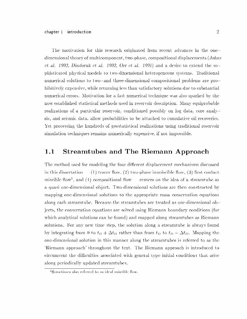
This chapter presents the main objective of the streamtube approach and the mo-
tivations that led to this research. The principal idea of using streamtubes as one-
dimensional systems, the Riemann approach for mapping solutions along streamtubes,
and the issue of nonlinearity in the problem formulation are brie y reviewed. The
class of problems for which the streamtube technique is applicable and its limitations
are discussed, and a brief overview of each chapter is given.
The primary objective of the streamtube approach is to enable fast and accurate
numerical solutions to displacements through strongly heterogeneous systems while
retaining the details of the underlying physical models seen in one-dimensional solu-
tions. The fundamental assumption in using the streamtube approach rests on the
belief that �eld scale displacements are dominated by reservoir heterogeneity: by cap-
turing ow paths and their relative importance as one-dimensional transport conduits
between wells while honoring the physical displacement mechanism along these con-
duits allows di�cult enhanced oil recovery displacements to be modeled successfully.
Fast and slow ow regions in the reservoir can be represented using quasi one-
dimensional streamtubes. Streamtubes can be visualized as an array of pipes, having
variable geometries and connecting the injector and producer wells. The shape of
each pipe (streamtube) is dictated by the reservoir geology and, most importantly,
each pipe is assumed to conserve mass: what goes in a pipe must come out.
1
chapter 1 introduction 2
The motivation for this research originated from recent advances in the one-
dimensional theory of multicomponent, two-phase, compositional displacements (Johns
et al. 1992, Dindoruk et al. 1992, Orr et al. 1991) and a desire to extend the so-
phisticated physical models to two-dimensional heterogeneous systems. Traditional
numerical solutions to two- and three-dimensional compositional problems are pro-
hibitively expensive, while returning less than satisfactory solutions due to substantial
numerical errors. Motivation for a fast numerical technique was also sparked by the
now established statistical methods used in reservoir description. Many equiprobable
realizations of a particular reservoir, conditioned possibly on log data, core analy-
sis, and seismic data, allow probabilities to be attached to cumulative oil recoveries.
Yet processing the hundreds of geostatistical realizations using traditional reservoir
simulation techniques remains numerically expensive, if not impossible.
1.1 Streamtubes and The Riemann Approach
The method used for modeling the four di�erent displacement mechanisms discussed
in this dissertation | (1) tracer ow, (2) two-phase immiscible ow, (3) �rst contact
miscible ow1, and (4) compositional ow | centers on the idea of a streamtube as
a quasi one-dimensional object. Two-dimensional solutions are then constructed by
mapping one-dimensional solutions to the appropriate mass conservation equations
along each streamtube. Because the streamtubes are treated as one-dimensional ob-
jects, the conservation equations are solved using Riemann boundary conditions (for
which analytical solutions can be found) and mapped along streamtubes as Riemann
solutions. For any new time step, the solution along a streamtube is always found
by integrating from 0 to tD + �tD rather than from tD to tD + �tD. Mapping the
one-dimensional solution in this manner along the streamtubes is referred to as the
`Riemann approach' throughout the text. The Riemann approach is introduced to
circumvent the di�culties associated with general type initial conditions that arise
along periodically updated streamtubes.
1Sometimes also referred to as ideal miscible ow.
chapter 1 introduction 3
1.2 Nonlinearity
The fundamental di�culty in solving the partial di�erential equations (PDE's) gov-
erning the ow through porous media is their nonlinear formulation. In other words,
in order to account for the relevant physics of uid ow, the coe�cients that appear
in the governing equations (relative permeabilities, viscosities, densities, etc...) be-
come functions of the independent variables of the problem, usually phase saturations
and/or overall compositions. A special case occurs when the coe�cients are assumed
constant with respect to the independent variables2, as is done in unit mobility ratio
(M=1) ow. In that case the streamtubes are �xed with time and the ow is said to
be linear.
To account for the inherent nonlinearity of all other displacements, the stream-
tube approach periodically updates the streamtubes (i.e. solves the elliptic PDE for
the streamfunction) and maps the one-dimensional solution to the particular trans-
port problem onto the new streamtubes using the Riemann approach. Thus, the
term `nonlinearity' is used in this dissertation to describe the changing velocity �eld
with time, as re ected by the dependence of the total mobility on saturation and/or
compositions in the elliptic PDE for the streamfunction.
1.3 Class of Problems
The streamtube approach is meant to solve problems that are dominated by reservoir
heterogeneity and convective forces. Only cross-sectional problems are discussed here,
although there are no dimensional limitations and the method can be used in areal,
multiwell con�gurations as well as in three dimensions3. Solutions by the stream-
tube approach discussed in this dissertation are restricted to problems with constant
initial and injected conditions (Riemann boundary conditions) and no gravity-driven
2Although the coe�cients (like permeability) may still vary spatially.3Although not as easily derived as in two-dimensions, three dimensional streamtubes arise by con-
sidering the intersection of stream surfaces (Bear 1972, p.226). Once a three-dimensional streamtubeis de�ned, all the arguments with regard to mapping one-dimensional solutions along a streamtubein two dimensions can be applied directly to a streamtube in three dimensions.
chapter 1 introduction 4
ow. Finally, the one-dimensional nature of the streamtubes requires transverse ow
mechanisms (normal to the streamtube boundaries) to be of negligible importance.
1.4 Outline
Chapter 2 outlines the relevant literature on streamlines and streamtubes. The pri-
mary emphasis is on the petroleum literature, which has seen repeated applications
of streamline and streamtube methods, beginning with Muskat and Wycko� (1934)
who were among the �rst to use streamlines to study how well patterns would af-
fect oil recovery. The groundwater literature is brie y reviewed as well, although
a comprehensive coverage is traded for key publications that may serve as anchor
points to the vast body of literature dealing with the subject. The boundary element
method is reviewed as an alternative and e�cient method to generate streamlines,
and front tracking is presented as a related method to the streamtube approach in
moving discontinuous solutions along streamlines.
Chapter 3 introduces the mathematical model for simulating uid ow through
porous media using streamtubes. The governing PDE for the streamfunction in het-
erogeneous media is discussed, and the resulting streamtubes are presented as pseudo
one-dimensional systems. The key issue of mapping one-dimensional solutions along
streamtubes is discussed.
Chapter 4 applies the streamtube approach to unit mobility (tracer) displace-
ments. A piston-like, one-dimensional solution is mapped along streamtubes to give a
numerical-di�usion-free, two-dimensional solution for a heterogeneous domain. Phys-
ical longitudinal di�usion is added to the solution by mapping the convection-di�usion
equation along streamtubes. The error caused by numerical di�usion in traditional
�nite di�erence approaches is quanti�ed using the di�usion-free streamtube solution
as reference solution.
Chapter 5 solves the two-phase immiscible problem by mapping the well-known
Buckley-Leverett solution along streamtubes. The issue of the inherent nonlinearity
in the velocity �eld is solved by periodically updating the streamtubes and remapping
the Buckley-Leverett solution using the Riemann approach. The Riemann approach
chapter 1 introduction 5
is validated and shown to introduce smaller errors than numerical di�usion in tradi-
tional �nite di�erence simulators. It is also compared to the Higgins and Leighton
method in which the streamtubes are �xed throughout the displacement and rates
are allocated according to the total ow resistance of each streamtube. The key result
of this chapter is the demonstration that two-phase immiscible displacements can be
successfully modeled using two-orders of magnitude fewer matrix inversions than tra-
ditional �nite di�erence simulators. The superior speed is then put to use to assess
the interaction of nonlinearity and reservoir heterogeneity in de�ning the uncertainty
in cumulative recovery.
Chapter 6 looks at solving �rst contact miscible displacements (FCM) by mapping
three possible one-dimensional solutions along streamtubes: (1) a piston-like solution,
(2) a convection-di�usion solution, and (3) a viscous �ngering solution. The important
issue of scale is discussed given that viscous �ngering cannot be represented explic-
itly and is captured at the sub-streamtube scale by using a Todd{Longsta� model.
Streamtubes are assumed to be on a �eld scale, attaining a Fickian limit within each
streamtube for M = 1 ow while giving rise to viscous �ngering for M > 1. The
streamtube approach is shown to match overall recoveries obtained using Mistress, a
�nite di�erence code with a ux-corrected-transport formulation (Christie and Bond
1985), with a speed-up by two to three orders of magnitude. Ninety geostatistical real-
izations with di�erent heterogeneity indices (HI = 0:077; 0:18; 0:86 |30 realizations
per HI) are used in 180 displacements (M = 5 and M = 10) to demonstrate that
increasing heterogeneity and increasing nonlinearity combine to increase substantially
the uncertainty in recovery.
Chapter 7 applies the streamtube approach to compositional displacements through
heterogeneous systems. One-dimensional as well as two-dimensional reference solu-
tions are found numerically using a �nite di�erence compositional simulator (UT-
COMP ). By comparing the di�usion-free streamtube solutions to the UTCOMP solu-
tions, numerical di�usion is shown to reduce substantially the original instability of
the displacement. Streamtube solutions are made to match the UTCOMP solutions
by completely eliminating the mobility contrast, i.e. setting M = 1. The result-
ing speed-up is by four to �ve orders of magnitude. Cross ow is not found to be a
chapter 1 introduction 6
dominant factor in mitigating the displacements for the heterogeneous systems inves-
tigated here, and the e�ect of cross ow is argued to be on the order of transverse
di�usion.
Finally, Chapter 8 gives a brief summary of the dissertation, points out the limita-
tions of the streamtube approach, and identi�es the main conclusions of this research.
Chapter 2
Literature Review
This chapter reviews the relevant literature on streamlines and streamtubes, with
particular emphasis on the petroleum literature. Brief reviews of the groundwater
literature, the boundary element method (an alternative approach for generating
streamlines), and the front-tracking method are presented as well.
2.1 Introduction
Streamlines and streamtubes are well established in computational uid dynamics
and have given rise to a very large body of literature. This chapter reviews ideas
and concepts in the published literature involving streamlines/streamtubes which are
directly related to modeling of subsurface uid ow.
Unfortunately, the groundwater and petroleum literatures have evolved quite inde-
pendently from each other and little cross referencing has taken place on the general
subject of streamlines and streamtubes. In part, this is due to the di�erence in
the fundamental problem the two �elds are concerned with: regional, single-phase
ow with emphasis on aquatic chemistry in groundwater mechanics versus con�ned,
multiphase, multicomponent ow in petroleum engineering. This chapter is biased
towards the petroleum literature, although it is fair to say that the concepts of
streamlines/streamtubes are probably better established in the groundwater liter-
ature. Textbooks on groundwater ow (e.g. Bear 1972, Strack 1989) usually include
a discussion on streamlines and streamtubes as a modeling technique, whereas it is
7
chapter 2 literature review 8
rare to �nd these ideas discussed in petroleum engineering text books1.
Two main issues arise in modeling multiphase displacements in porous media
streamtubes: (1) generating streamlines/streamtubes for a particular geometry and
reservoir heterogeneity and (2) accounting for the inherent nonlinearity in the ow
�eld. Streamtubes are generally found by solving for the pressure �eld and then
tracing streamlines using the derived velocity �eld. An alternative is given by the
boundary element method (BEM), which has a high degree of accuracy and leads
to a smaller system of algebraic equations, although it has di�culties in handling
heterogeneous domains. The nonlinearity in the velocity �eld is usually accounted
for by �xing the streamtubes in time (i.e. solving the velocity �eld only once) and
then modifying the ow rate associated with each streamtube according to the total
resistance of the system as a function of time. A more rigorous, but somewhat involved
approach, is the front-tracking method; the velocity �eld is recalculated periodically
and the saturation/concentration fronts are moved according to their characteristic
velocities.
In reviewing the relevant literature, a chronological order is used to highlight
original contributions by the authors as well as to maintain the natural succession
of ideas. Brief summaries of some of the papers discussed here can be found in
Appendix B.
2.2 Petroleum Literature
As with many subjects in reservoir engineering, Muskat was one of the �rst to apply
streamlines to study how well patterns would a�ect recovery (Muskat and Wycko�,
1934). Using electrical conduction models, Muskat and Wycko� compare the recovery
e�ciency of a staggered line drive, a direct line drive, a �ve-spot pattern, and a seven-
spot pattern, �nding the staggered line drive as having `the most favorable physical
features'. They discuss their results in terms of two-phase ow, although tracer- ow
assumptions are used for all calculations. Thus, the streamlines are assumed �xed in
time. An interesting note is that Muskat and Wycko� conclude their discussion by
1An exception is the book by Muskat (1937): The Flow of Homogeneous Fluids.
chapter 2 literature review 9
suggesting that, all things considered, well spacing and arrangement may be of minor
importance compared to the channeling caused by `high permeability zones within
the main body of sand', an idea that is clearly in line with current beliefs on the
importance of reservoir heterogeneity in determining recovery.
Muskat devotes an entire chapter in his famous textbook, Flow of Homogeneous
Fluids (Muskat 1937), to two-dimensional problems that can be analyzed using po-
tential-theory methods. These methods rely on the analogy between the equations
describing steady state current ow in an electrolytic medium and the equations de-
scribing steady-state uid ow in porous media and are used to capture the stream-
lines resulting from the geometrical constraints imposed by the boundaries and wells
(Lee 1948). Muskat (Muskat 1948) extends the potentiometric approach to account
for reservoir heterogeneity by demonstrating that varying the electrolyte layer thick-
ness is equivalent to specifying a spatial kh distribution.
Higgins and Leighton are credited with being the �rst to apply the streamtube
technique to model nonlinear displacements in homogeneous, areal domains for sev-
eral regular well patterns. Their work is discussed in three publications: Higgins and
Leighton (1962a) discusses two-phase ow, Higgins and Leighton (1962b) considers
three-phase ow, and Higgins et al. (1964) studies the in uence of several di�erent
well patterns. In their �rst paper, Higgins and Leighton consider a homogeneous
quarter �ve-spot pattern in which ten streamtubes are divided into `sand elements' of
equal volume. By determining the average mobility (actually referred to as average
permeability in the paper) and a `geometric shape factor' for each sand element at the
end of each time step, Higgins and Leighton �nd the total resistance of each stream-
tube (`channel'). The amount of uid injected into each streamtube is then allocated
proportionally to the ratio of the resistance of each streamtube to the total resistance
of the system. Although the streamtubes are �xed throughout the displacement,
Higgins and Leighton show excellent agreement with laboratory water ood data re-
ported by Douglas et al. (1959) for end-point viscosity ratios ranging from 0.083 to
754. It is important to note however, that in all cases the relative permeability curves
(`permeability-saturation curves') used by Higgins and Leighton in their simulations
give rise to rarefaction waves only. In other words, although the end-point mobility
chapter 2 literature review 10
ratio is very high, the instability is mitigated across a very long rarefaction wave. Hig-
gins and Leighton (9/1962b) then extend their approach to three-phase ow by using
the water-oil fractional ow to �nd the two-phase mixed-wave solution and assuming
that the gas has in�nite mobility such that it will always travel ahead of the water-oil
region. Although the one-dimensional three-phase ow assumptions are questionable,
Higgins and Leighton show a good match with a layered system. Finally, Higgins et
al. (1964) extend the Higgins and Leighton method to several production patterns,
including a seven-spot, a direct line-drive, and a staggered line-drive and provide the
reader with a table of shape factors for the various cases.
Hauber (1964) derives analytical expressions for calculating injectivity, time, and
cumulative water injected when the water-oil interface has moved a given distance
along a streamtube and introduces a distortion factor for non-unit mobility ratio dis-
placements to account for changing streamtube geometries as the ood progresses.
Hauber applies his method to a �ve spot and direct line drive. He then compares
his results to experimental data obtained from an electrolytic model and X-ray shad-
owgraph model, as well as a moving interface algorithm proposed by Sheldon and
Dougherty (1964). Reasonable agreement with experimental data and the moving
interface algorithm is shown.
An important extension to the Higgins and Leighton method is presented byDoyle
and Wurl (1971). Doyle and Wurl apply the streamtube approach to �elds that have
asymmetrical well patterns and irregular boundaries. They use superposition to �nd
the streamlines and proceed to �nd the geometrical shape factors for each streamtube
allowing them to apply the Higgins and Leighton method. Unfortunately, Doyle and
Wurl never actually discuss the algorithm they use to introduce the �eld boundaries
in their streamline generation. The contribution by Doyle and Wurl is to extend
the streamtube method to real �eld geometries and to set the stage for a number of
papers to follow by other authors, which use streamtubes to model real �eld cases.
LeBlanc and Caudle (1971) also use superposition of line sources and sinks to
generate streamlines for a homogeneous domain, but do away with the geometrical
shape factors necessary in the Higgins and Leighton method by noting that the total
uid velocity along the dividing streamline is known if each streamtube is assumed
chapter 2 literature review 11
to carry the same injection rate. Instead of using a geometrical approach, LeBlanc
and Caudle integrate along each streamline to capture the variation in total velocity.
Parsons (1972) was the �rst to consider permeability anisotropy. He shows how
ow patterns can be substantially altered leading to much lower recoveries than in the
isotropic cases. It is interesting to note that Parsons uses a time-of- ight coordinate
along streamlines, thereby de�ning a ood front as points having an equal time-of-
ight value. In fact, a similar variable was used by Muskat (Muskat 1948) to de�ne
`constant time surfaces'.
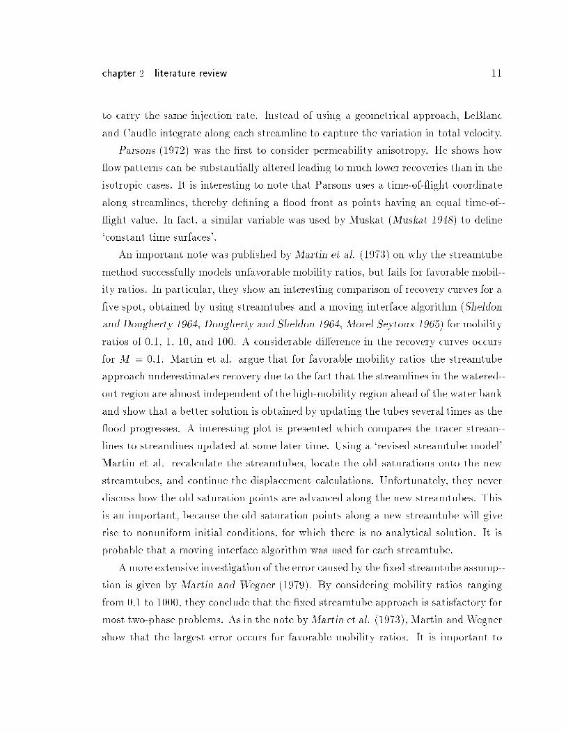
An important note was published by Martin et al. (1973) on why the streamtube
method successfully models unfavorable mobility ratios, but fails for favorable mobil-
ity ratios. In particular, they show an interesting comparison of recovery curves for a
�ve spot, obtained by using streamtubes and a moving interface algorithm (Sheldon
and Dougherty 1964, Dougherty and Sheldon 1964, Morel-Seytoux 1965) for mobility
ratios of 0.1, 1, 10, and 100. A considerable di�erence in the recovery curves occurs
for M = 0:1. Martin et al. argue that for favorable mobility ratios the streamtube
approach underestimates recovery due to the fact that the streamlines in the watered-
out region are almost independent of the high-mobility region ahead of the water bank
and show that a better solution is obtained by updating the tubes several times as the
ood progresses. A interesting plot is presented which compares the tracer stream-
lines to streamlines updated at some later time. Using a `revised streamtube model'
Martin et al. recalculate the streamtubes, locate the old saturations onto the new
streamtubes, and continue the displacement calculations. Unfortunately, they never
discuss how the old saturation points are advanced along the new streamtubes. This
is an important, because the old saturation points along a new streamtube will give
rise to nonuniform initial conditions, for which there is no analytical solution. It is
probable that a moving interface algorithm was used for each streamtube.
A more extensive investigation of the error caused by the �xed streamtube assump-
tion is given by Martin and Wegner (1979). By considering mobility ratios ranging
from 0:1 to 1000, they conclude that the �xed streamtube approach is satisfactory for
most two-phase problems. As in the note byMartin et al. (1973), Martin and Wegner
show that the largest error occurs for favorable mobility ratios. It is important to
chapter 2 literature review 12
mention that in all unfavorable mobility ratio cases, the relative permeability curves
used by Martin and Wegner give rise to rarefaction waves only (as in the case for Hig-
gins and Leighton), which also explains why their M = 1000 comparison on p. 314
shows such good agreement. Martin and Wegner also mention how the problem of
numerical di�usion is overcome by using streamtubes, but do not attempt to quantify
this advantage.
An interesting application of streamtubes to modeling in-situ uranium leaching is
presented byBommer and Schechter (1979). For this particular case, the unit mobility
displacement involved justi�es the constant streamtube assumption. The original
contribution by Bommer and Schechter is to solve the conservation equations using
a one-dimensional �nite di�erence formulation along each streamtube. Using this
approach, they are able to account for chemical reactions and physical di�usion in the
main direction of ow, thereby modeling the relevant physics of the leaching process.
The streamlines are found analytically using superposition, with the no- ow �eld
boundary de�ned by image wells placed accordingly. A very similar application for
a micellar/polymer ood is presented by Wang et al. (1981). A streamline generator
sets up the ow �eld and then the concentration balance is solved by �nite di�erence
along each �xed streamline.
An important step forward in the attempt to include heterogeneity in the displace-
ment calculations is due to Lake et al. (1981). Using physical data from laboratory
experiments along with a layered geological model, Lake et al. generate a detailed,
vertical cross-sectional �nite di�erence solution for a polymer ood, which is then col-
lapsed into an average one-dimensional solution and mapped onto areal streamtubes
to obtain a three-dimensional �eld response. The importance of this paper lies in
the novel idea of introducing the interaction of heterogeneity with the physics of the
surfactant/polymer displacement by decoupling the vertical response from the areal
one. The main assumption in the method proposed by Lake et al. is that the areal
ow �eld is primarily in uenced by well placement, whereas the vertical response is
a strong function of geology and type of displacement. Lake et al. assume constant
streamtube injectivities in their calculations.
Abbaszadeh-Dehghani (1982) applies the streamtube approach to solve the inverse
chapter 2 literature review 13
problem. From breakthrough curves of tracer slug injections, Abbaszadeh-Dehghani
is able to reconstruct layered kh models that will honor the �eld data. He maps a
convection-di�usion solution onto the pattern of streamtubes and uses a nonlinear
optimization technique to converge onto the best layered model.
Emanuel et al. (1989) apply the powerful, hybrid streamtube technique proposed
by Lake et al. (1981) to determine the �eld performance of three CO2 oods and one
mature water ood. The cross-sectional response function is found by detailed �nite-
di�erence simulation using a fractal description of the porosity/permeability distri-
bution and core ood data. In determining the areal solution, Emanuel et al. account
for nonunit mobility ratios, permeability/thickness values, and no- ow boundaries.
For all cases, Emanuel et al. show excellent agreement with total �eld response data.
Other examples of the hybrid streamtube technique are given by Mathews et al.
(1989) (miscible-hydrocarbon WAG ood) and Tang et al. (1989) (a water ood and
a CO2 ood). The examples by Tang et al. are particularly interesting because in
determining the average cross-sectional response function, they varied the width of
the cross-section in the �nite di�erence simulation in order to capture the transition
from radial ow near the wells to linear ow away from the wells, thus including
gravity e�ects. Furthermore, Tang et al. generate ten di�erent fractional ow curves
to account for varying CO2 slug sizes, which results from updating the ow rates for
each streamtube as the ood progresses.
Motivated by the success of the hybrid streamtube approach, Hewett and Behrens
(1991) give a detailed discussion on scaling properties of hyperbolic conservation
problems and on determining average response functions (pseudofunctions) for het-
erogeneous cross sections. In particular, Hewett and Behrens show that for single
slug injections the solution is scalable by xD=tDs and tD=tDs, where tDs is the di-
mensionless slug volume. Since the hybrid streamtube method requires an averaged
cross-sectional response, Hewett and Behrens study the in uence of heterogeneity on
the scaling properties of a pseudo one-dimensional solution. They conclude that, in
general, heterogeneity does not allow a two-dimensional solution to be collapsed into
a one-dimensional solution that can be scaled by xD=tD, although in some special
cases the permeability correlation length may be used as an additional parameter to
chapter 2 literature review 14
give reasonably scaled solutions.
Renard (1990) departs from the assumption of constant streamtubes and allo-
cation of rates according to total resistance. Instead, he periodically updates the
streamtubes and maps the old saturations/concentrations onto the new streamtubes.
Renard presents a micellar/polymer example in which he compares �eld data with
�xed and updated streamtube solutions. The solution with updated streamtubes is
closer to the �eld data than the one using �xed streamtubes. Unfortunataly Renard
does not indicate how he actually moves the old saturations/concentrations along the
new streamtubes.
King et al. (1993) present a modi�ed streamline approach as a rapid technique
to evaluate the impact of heterogeneity on miscible displacements. A time-of- ight
coordinate is used to map the Todd{Longsta� model along each streamline, much
in the same way as Parsons (1972) does to locate the position of a tracer front. To
account for unfavorable mobility ratios, King et al. use a `boost' factor by integrating
Darcy's law along each streamline up to the isobar coinciding with the fastest �nger,
a slightly di�erent approach than that used by previous authors, who integrate over
the entire streamline.
2.3 Groundwater Literature
It is fair to say that the concepts of streamlines and streamtubes for modeling subsur-
face uid ow are well established in the groundwater literature. A testimony to this
fact is the considerable number of publications that deal directly or indirectly with
the streamfunction as well as the many textbooks that give a complete presentation of
the method (Bear 1972, Strack 1989). It would therefore be di�cult to give a formal
review of the subject without the danger of not citing many important contributions.
This section is principally an acknowledgment of the vast body of literature dealing
with streamlines and streamtubes in the groundwater literature. Its purpose is to
identify some key publications that will serve as a reference for a more comprehensive
coverage.
Streamlines and streamtubes are particularly suitable as a modeling technique for
chapter 2 literature review 15
groundwater ow given the steady state nature of many problems of concern to the
hydrogeologists. For example, the transport of contaminants by a regional ow �eld
is a steady-state problem that is probably best captured by a streamtube approach
as demonstrated by Nelson (1978) and Frind et al. (1985). A nice review of the
theory related to the streamtube approach is presented by Frind and Matanga (1985).
Frind et al. (1988) use the streamtube approach (`dual potential-streamfunction
formulation') to capture dispersive processes at di�erent scales that can in uence
the evolution of a plume as it migrates downstream in heterogeneous media. Local
scale di�usive processes are captured by using a local Peclet number in the convection-
di�usion equation, while larger-scale di�usion is represented through the resolution of
the ow �eld (streamtubes) and di�usive exchange between streamtubes. A variable
density formulation of the streamfunction is presented by Evans and Ra�ensperger
(1992), which they use to model ow near a salt dome. They show that in the case
of gravity driven, single-phase ow the streamfunction should be derived in terms of
mass ux rather than volume ux. Finally, several authors present extension of the
streamtube method to three-dimensions (Matanga 1993, Zijl 1986, Bear 1972, and
Yih 1957).
2.4 Boundary Element Methods
The use of streamtubes to generate solutions for particular displacement processes
rests on the ability to generate streamlines for a particular reservoir geometry and
con�guration of wells. Streamlines can be found by either solving for the pressure
distribution and then using Darcy's law to �nd the ow �eld and the resulting stream-
lines by tracing a particle from a source to sink, or by solving for the streamfunction
directly. If the reservoir is homogeneous and the well pattern is symmetric and re-
peatable to in�nity, superposition can be used to �nd explicit expressions for the
velocity vector anywhere in the reservoir (Muskat 1937, LeBlanc and Caudle 1971,
Wang et al. 1981). On the other hand, if the reservoir has an irregular boundary
placing image wells so as to honor the reservoir boundary becomes di�cult and a
trial-and-error solution is necessary (Lin 1972).
chapter 2 literature review 16
An interesting and e�cient alternative to generate streamlines, particularly for
domains with an arbitrary boundary, is provided by the boundary element method
(BEM). The BEM rests on Green's second identity and features a number of advan-
tages over the conventional �nite di�erence method (Masukawa and Horne, 1988): (a)
discretization errors occur on the boundary only, thereby reducing numerical di�usion
and grid orientation e�ects, (b) there are few restrictions on �eld geometries, (c) a
reduction of the problem dimensionality by one (3D problems are reduced to 2D, 2D
problems to 1D), and (d) the ow potential and velocity can be determined for any
point in the domain. A number of authors have presented applications of the BEM
method to solve subsurface uid ow problems. Liu et al. (1981) solves a moving
interface problem and present numerical and experimental results for the tilting of
a vertical interface in a Hele-Shaw cell. Lafe et al. (1981) extend the BEM method
to solve nonlinear equations and equations that have nonconstant coe�cients. Both,
Cheng (1984) and Lafe and Cheng (1987) develop the BEM method for heterogeneous
domains.
Applications of the BEM to reservoir engineering are also presented byMasukawa
and Horne (1988) who apply it to immiscible displacement problems. Numbere and
Tiab (1988) present the BEM methods as an improved streamline generating tech-
nique, while Sato (1992), and Sato and Horne (1993) use a perturbation approach to
solve steady-state and transient ow problems in heterogeneous domains. An elegant
application of the BEM to track streamlines across fractures is presented by Sato and
Abbaszadeh (1994).
Although powerful, the BEMmethod has been slow to gain acceptance in petroleum
engineering research, probably due to its involved mathematical formulation and its
limitations in handling heterogeneous domains. Sato and Horne (1993) use regular
perturbation methods to decompose the underlying equations for the heterogeneous
case and are able to obtain streamlines. Nevertheless, they caution against slow
convergence and divergence of the perturbation series as the magnitude of spatial
variability increases.
chapter 2 literature review 17
2.5 Front Tracking
A related method to the streamtube approach is the front tracking method. The
central idea of the front tracking method is to move fronts with their characteristic
velocities along streamlines, thereby retaining saturation discontinuities (shocks) that
arise in the solutions of hyperbolic conservation equations.
Sheldon and Dougherty (1964), Dougherty and Sheldon (1964), andMorel-Seytoux
(1965) introduced the idea of front-tracking (sometimes referred to as moving inter-
face method) to the petroleum literature. Sheldon and Dougherty discuss the general
idea of moving a single uid interface with time and Dougherty and Sheldon then
apply these ideas to a water ood in which the 1D saturation pro�le is treated as a
series of fronts. Morel-Seytoux introduces an `analytical-numerical' method in which
the streamlines are found analytically for the unit mobility ratio case and then used
to �nd a scale-factor in the frontal advance equations.
More recent applications of the front tracking approach are due to Glimm et al.
(1983), Ewing et al. (1983), and Bratvedt et al. (1989). The approach presented
by Bratvedt et al. is particularly interesting because it directly relates to the idea
of updating streamtubes in nonlinear displacements (Martin et al. 1973, Renard
1990) and moving saturation along new streamtubes. In particular, Bratvedt et
al. use a piecewise linear approximation of the fractional ow function, which leads
to a saturation pro�le that is piecewise constant, in the same manner as assumed
by Dougherty and Sheldon (1964). Each saturation front is then considered as a
local Riemann problem and can be moved forward in time by using its characteristic
velocity. Bratvedt et al. are able to account for colliding fronts and apply their
method to �eld scale problems with good results.
2.6 Concluding Remarks
A substantial amount of work has been done in trying to use streamlines and stream-
tubes as a predictive tool for �eld scale displacements. Nevertheless, much room for
improvement remains, particularly in trying to account for reservoir heterogeneity
chapter 2 literature review 18
and the inherent nonlinearity in the velocity �eld for unstable displacements. This
work extends the streamtube method to consider these issues. Cross-sectional do-
mains are used emphasizing reservoir heterogeneity, and streamtubes are updated
periodically to account for nonlinear behavior. Solutions for various displacement
mechanisms are then constructed by treating streamtubes as true one-dimensional
systems along which mass conservation solution(s) can be mapped, thus retaining
the essential physics of ow. A `Riemann approach' is used to map one-dimensional
solutions along periodically updated streamtubes; this is di�erent from any previous
streamtube/streamline methods and is introduced to allow the use of one-dimensional
Riemann solutions along changing streamtubes. As a result, the streamtube method
becomes particularly powerful in the case of compositional solutions, where one-
dimensional solutions containing all the relevant physics are combined with stream-
tubes to produce very fast and accurate displacement predictions for heterogeneous
systems.
Chapter 3
Mathematical Model
This chapter introduces the mathematical model for simulating uid ow through
porous media using streamtubes. The streamfunction for two-dimensional, heteroge-
neous media is derived and the appropriate boundary conditions presented. The con-
cept of a streamtube as a pseudo one-dimensional system is introduced, and the map-
ping of a one-dimensional solution onto streamtubes to construct a two-dimensional
solution is discussed.
3.1 Introduction
The streamtube approach rests on two key ideas: (a) generating streamlines and
streamtubes for the particular domain of interest and (b) mapping of a one-dimensional
solution along each streamtube. These central ideas, and the key assumptions asso-
ciated with them, are developed in this chapter.
The streamfunction is discussed in several textbooks (Muskat 1937, Bear 1972,
Strack 1989), and for a general discussion the reader is referred to these sources. In
this chapter, the governing partial di�erential equation for the streamfunction and
the appropriate boundary conditions are derived for a cross-sectional heterogeneous
domain. Injection is assumed to occur over the entire left face of the domain and
production over the entire right face. The top and bottom boundaries are treated as
no- ow boundaries.
The choice of a cross-sectional domain is motivated by the interest to understand
19
chapter 3 mathematical model 20
the e�ects of heterogeneity on nonlinear displacement processes. Furthermore, in a
cross-sectional domain the streamlines can be solved for directly and very easily. In
the case of areal problems with multiple wells, the streamfunction can still be used
although it becomes multivalued and branch cuts (bounding streamlines) must be
found (Emmanuel et al. 1989). For these cases it may be easier to determine the
pressure distribution and combine it with Darcy's Law to �nd the underlying total
velocity �eld and trace streamlines by launching particles.
3.2 The Streamfunction - Constant Coe�cients
By de�nition, a streamline is a line everywhere tangent to the velocity vector (Muskat
1937, Bear 1972, Strack 1989) at any instant in time. In parametric form, a streamline
can be written as
x = x(s) ; y = y(s) :1 (3:1)
The slope of a velocity vector anywhere along a streamline is given by
dy=ds
dx=ds=
uy
ux;
which can be rearranged as
uydx
ds� ux
dy
ds= 0 : (3:2)
ux and uy are the Darcy velocity components in the x and y direction respectively.
Consider now a function , called the streamfunction. If the streamfunction is
required to be constant along a streamline, then it must hold that
d =@
@x
dx
ds+@
@y
dy
ds= 0 : (3:3)
1Streamlines, of course, exist in unsteady ow as well: x = x(s; t) ; y = y(s; t). In this caseone distinguishes between pathlines, streamlines, and streaklines. The pathline is the locus of aparticle in space as time passes; a streamline is a line everywhere tangent to the velocity vector;and a streakline is the locus of all points seen by a uid particle that passed through a �xed pointspace at some earlier time (Bear 1972). In steady state ow pathlines, streamlines, and streaklinescoincide, whereas in unsteady state ow they do not.
chapter 3 mathematical model 21
Comparisons of terms with Eq. 3.2 gives
@
@x= uy ;
@
@y= �ux ; (3:4)
and substituting for ux and uy using Darcy's law returns
@
@x= �
@P
@y;
@
@y= ��@P
@x;
where � is the mobility of the uid. Assuming that � is spatially constant (homo-
geneous uid and rock properties) it can be taken into the partial derivatives such
that@
@x=@(�P )
@y;
@
@y= �@(�P )
@x
and setting � = �P gives
@
@x=@�
@y;
@
@y= �@�
@x: (3:5)
Equations 3.5 are the well known Cauchy-Riemann equations2 that arise in the study
of functions of a complex variable (Churchill and Brown 1990).
In particular, if a function f(z) = u(x; y)+iv(x; y) of a complex variable z = x+iy
is said to be analytic, then the Cauchy-Riemann equations will hold for the functions
u and v:3 ux = vy and uy = �vx. The function f(z) is analytic if its derivative,
f 0(z), exists everywhere in the domain D. The importance of analytic functions for
modeling uid ow hinges on the fact that if f (z) is analytic inD, then its component
functions u and v are harmonic in D. Harmonic functions are functions that satisfy
Laplace's equation. Thus, if f (z) = u(x; y) + iv(x; y) is analytic, then u and v will
satisfy the Cauchy-Riemann equations as well as
uxx + uyy = 0 ; vxx + vyy = 0:
In uid ow through porous media an analytic function is referred to as the complex
2The Cauchy-Riemann equations are named after the French mathematician A.L. Cauchy (1789-1857) who discovered and used them, and after the German mathematician G.F.B. Riemann (1826-1866), who used them in the development of the theory of functions of a complex variable.
3Here u is simply used as a function name and is not to be confused with the Darcy's velocity.

chapter 3 mathematical model 22
potential (Muskat 1937, Bear 1972, Strack 1989) and written as
(x; y) = �(x; y) + i(x; y) ; (3:6)
where � is the potential function and is the streamfunction. Thus, a complex
potential that is analytic in D will give the governing partial di�erential equation
for the streamfunction as simply
@2
@x2+@2
@y2= 0 : (3:7)
For some homogeneous domains can be found analytically using conformal mapping.
� and , of course, give rise to the well known orthogonal ow nets that are widely
used in hydrology.
3.3 The Streamfunction - Variable Coe�cients
For this work, the interest lies in deriving the governing partial di�erential equation for
the streamfunction which accounts for reservoir heterogeneity and spatially varying
uid properties (relative permeabilities and viscosities). Substituting for Darcy's law
in Eq. 3.4, gives@
@x= ��y
@P
@y;
@
@y= �x
@P
@x; (3:8)
where �x and �y now are the total uid mobilities in the x and y direction and given
by
�x =NpXj=1
kxkrj
�j; �y =
NpXj=1
kykrj
�j: (3:9)
j is the phase index, Np is the total number of phases present, kx and ky are the abso-
lute permeabilities in the x and y direction respectively, krj is the relative permeability
of phase j, and �j is the viscosity of phase j. The phase relative permeabilities krj
and phase viscosities �j are indirect functions of x and y since they depend on phase
saturations/compositions which in turn are functions of x and y.
Eqs. 3.8 are still Cauchy-Riemann equations and can be expressed as
1
�y
@
@x= �@P
@y;
1
�x
@
@y=@P
@x: (3:10)
chapter 3 mathematical model 23
It is important to note that the Cauchy-Riemann equations alone are not a su�-
cient condition for the existence of an analytical function. Rather,a function f(z) =
u(x; y) + iv(x; y) is analytic in a domain D if and only if v is a harmonic conjugate
of u in D. In other words, to �nd the complex potential = P + i�, where the bar
indicates that � is now related to by
@ �
@x=
1
�y
@
@x;
@ �
@y=
1
�x
@
@y:
it must hold that@
@x
1
�y
@
@x
!+
@
@y
1
�x
@
@y
!= 0 : (3:11)
and � must be a harmonic conjugate of P (Bear 1972).
Eq. 3.11 is the governing pde for the streamfunction and accounts for reservoir
heterogeneity through its nonconstant spatial coe�cients. In practice the complex
potential is never found and usually only one of the component functions is used
for displacement calculations4. In this work, the streamfunction is the function of
interest and solved by applying Eq. 3.11 to a particular domain D.
A second, very simple derivation leading to Eq. 3.11 as well, begins by stating
that P is a single-valued function in D (Martin and Wegner 1979). Then the mixed
partials of P must be equal leading to
@
@x
@P
@y
!=
@
@y
@P
@x
!; (3:12)
and substituting for the pressure gradients from the Cauchy-Riemann equations
(Eqs. 3.8) gives@
@x
� 1
�y
@
@x
!=
@
@y
1
�x
@
@y
!; (3:13)
4The same argument used to �nd can be used to �nd P . In this case, the Cauchy-Riemannequations are written as
@
@x= ��y
@P
@y;
@
@y= �x
@P
@x;
the complex potential is given by = �P + i and the governing pde for P is
@
@x
��x
@P
@x
�+
@
@y
��y
@P
@y
�= 0 :

chapter 3 mathematical model 24
which returns the same governing equation for the streamfunction as Eq. 3.11
@
@x
1
�y
@
@x
!+
@
@y
1
�x
@
@y
!= 0 :
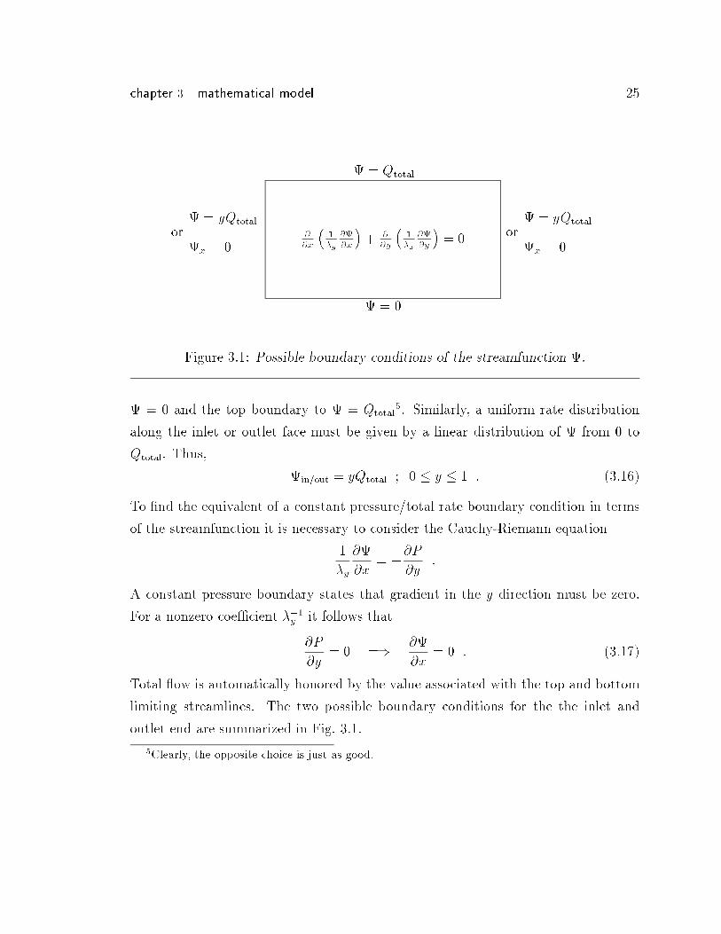
3.4 Boundary Conditions
Equation 3.11 is an elliptic partial di�erential equation, which requires either Neu-
mann or Dirichlet type boundary conditions. Only cross-sectional domains are con-
sidered in this work, and therefore the boundary conditions to be considered are
no- ow at the top and bottom of the domain and constant pressure or uniform rate
at either end. The boundary conditions for the streamfunction are particularly easy
to formulate, once a physical interpretation is given to the streamfunction .
The volumetric owrate at any point in the domain can be written in di�erential
form as
dQ = ~u � d ~A ; (3:14)
where d ~A is an arbitrary area between two adjacent streamlines de�ned as d ~A =
~ez�d~s. ~ez is the unit vector perpendicular to the xy plane and ds is the length of d ~A.The total volumetric ow rate across an arbitrary area A, between two streamlines
A and B, is then simply given by (Bear 1972, p.226)ZB
A
~u � d ~A = �QAB =ZB
A
~u � (~ez � d~s)
=ZB
A
uxdy � uydx
=ZB
A
d = B �A (3.15)
In other words, the total ow rate between two streamlines is simply given by the
di�erence in value of the streamfunction associated with each streamline.
Using this fact, the boundary conditions for the cross sectional domain are in-
deed easy to �nd. Since the top and bottom no ow boundaries and are themselves
streamlines, the di�erence in the value of the streamfunction between the two must
equal to the total owrate. An obvious choice then is to set the bottom boundary to
chapter 3 mathematical model 25
@
@x
�1
�y
@
@x
�+ @
@y
�1
�x
@
@y
�= 0
= Qtotal
= 0
= yQtotal = yQtotal
orx = 0 x = 0
or
Figure 3.1: Possible boundary conditions of the streamfunction .
= 0 and the top boundary to = Qtotal5. Similarly, a uniform rate distribution
along the inlet or outlet face must be given by a linear distribution of from 0 to
Qtotal. Thus,
in=out = yQtotal ; 0 � y � 1 : (3:16)
To �nd the equivalent of a constant pressure/total rate boundary condition in terms
of the streamfunction it is necessary to consider the Cauchy-Riemann equation
1
�y
@
@x= �@P
@y:
A constant pressure boundary states that gradient in the y direction must be zero.
For a nonzero coe�cient ��1y
it follows that
@P
@y= 0 =) @
@x= 0 : (3:17)
Total ow is automatically honored by the value associated with the top and bottom
limiting streamlines. The two possible boundary conditions for the the inlet and
outlet end are summarized in Fig. 3.1.
5Clearly, the opposite choice is just as good.
chapter 3 mathematical model 26
3.5 Numerical Solution
The numerical solution of Eq. 3.11 in a heterogeneous domain with any of the bound-
ary conditions speci�ed in Fig. 3.1 is straightforward and well documented in the
literature (Aziz and Settari 1979). A standard �ve-point �nite di�erence formulation
is used to discretize Eq. 3.11 resulting in
Ai+1;j +Bi�1;j + Ci;j+1 +Di;j�1 � (A+B + C +D)i+1;j = 0 ; (3:18)
where the coe�cients A,B,C, and D are given by
A =1
�x2
1
�y
!i+1=2;j
; (3.19)
B =1
�x2
1
�y
!i�1=2;j
; (3.20)
C =1
�y2
�1
�x
�i;j+1=2
; (3.21)
D =1
�y2
�1
�x
�i;j+1=2
: (3.22)
In solving for the streamfunction using Eq. 3.18, it is important to notice that the
gradient of in the x-direction is associated with the reciprocal of the mobility in the
y-direction. This is di�erent, of course, from solving for pressure, where the gradient
of P in the x-direction is associated with the mobility in the x-direction. � in Eq. 3.19
- 3.22 is the total mobility and can never be equal to zero unless the block absolute
permeability is zero. The harmonic average is used to �nd the value at the internodal
points (i� 1=2; j � 1=2). As an example, the coe�cient A would be given by
A =1
�x2
�yi;j + �yi+1;j
2�yi;j�yi+1;j
!: (3:23)
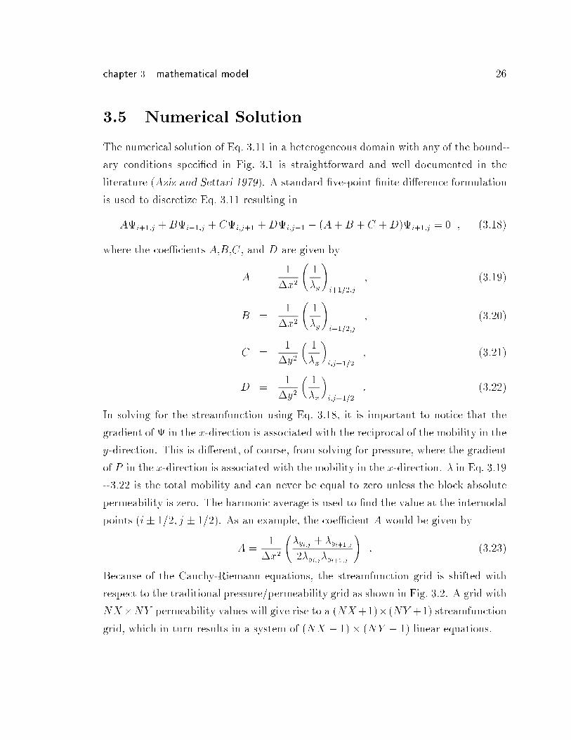
Because of the Cauchy-Riemann equations, the streamfunction grid is shifted with
respect to the traditional pressure/permeability grid as shown in Fig. 3.2. A grid with
NX�NY permeability values will give rise to a (NX+1)� (NY +1) streamfunction
grid, which in turn results in a system of (NX � 1)� (NY � 1) linear equations.
chapter 3 mathematical model 27
AA
Streamfunction Grid
Pressure/Permeability GridCauchy-Riemann Relations
In
Ψ = 0
Ψx = 0
Figure 3.2: Numerical grid for streamfunction in relation to the traditional block-centered pressure/permeability grid.
3.6 Streamtubes
Once the streamfunction has been solved for the particular heterogeneous domain of
interest, streamtubes are de�ned by considering two adjacent streamlines: N stream-
lines will de�ne N � 1 streamtubes.
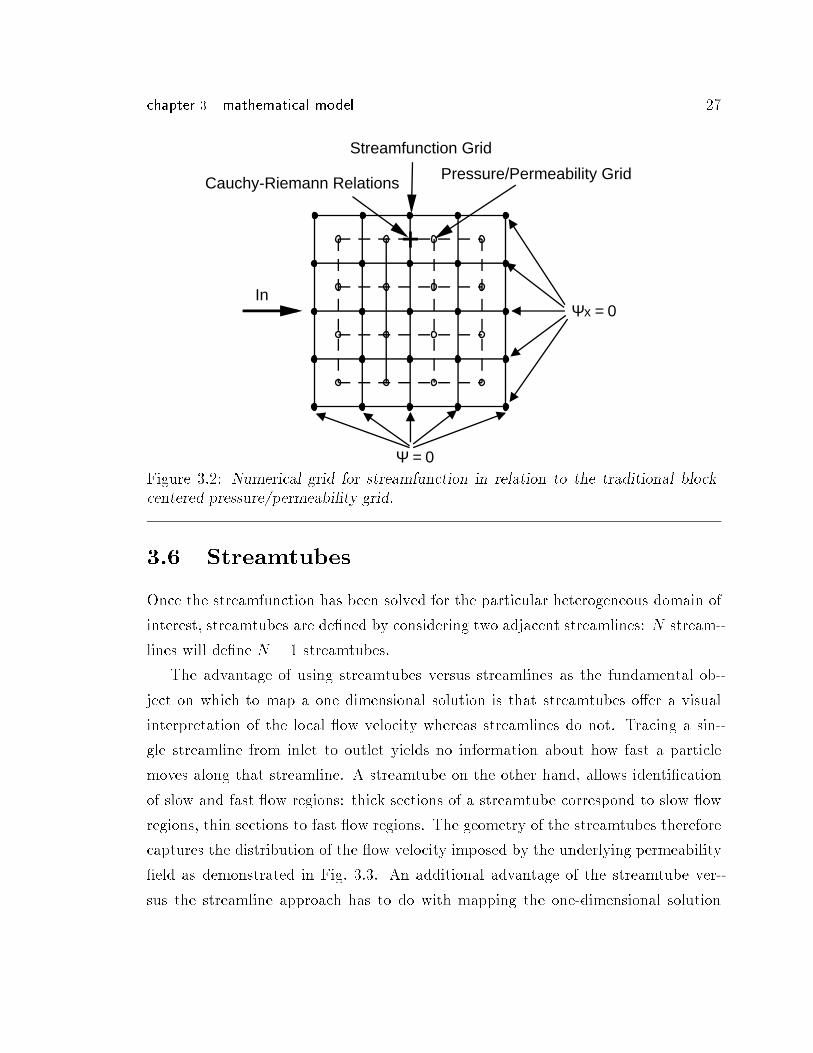
The advantage of using streamtubes versus streamlines as the fundamental ob-
ject on which to map a one dimensional solution is that streamtubes o�er a visual
interpretation of the local ow velocity whereas streamlines do not. Tracing a sin-
gle streamline from inlet to outlet yields no information about how fast a particle
moves along that streamline. A streamtube on the other hand, allows identi�cation
of slow and fast ow regions: thick sections of a streamtube correspond to slow ow
regions, thin sections to fast ow regions. The geometry of the streamtubes therefore
captures the distribution of the ow velocity imposed by the underlying permeability
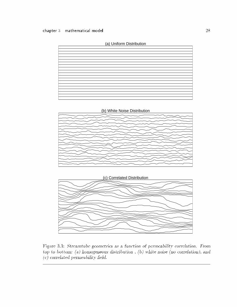
�eld as demonstrated in Fig. 3.3. An additional advantage of the streamtube ver-
sus the streamline approach has to do with mapping the one-dimensional solution
chapter 3 mathematical model 28
(a) Uniform Distribution
(b) White Noise Distribution
(c) Correlated Distribution
Figure 3.3: Streamtube geometries as a function of permeability correlation. From
top to bottom: (a) homogeneous distribution , (b) white noise (no correlation), and(c) correlated permeability �eld.
chapter 3 mathematical model 29
Ψ = 0
Ψ = 1
Streamline
NX+1 Interpolation Planes
Ψ = 0.5
Ψ = 0.6
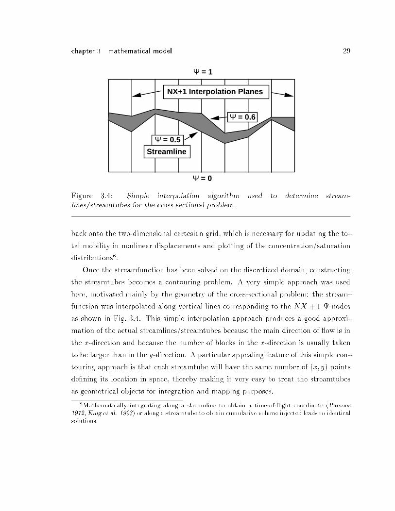
Figure 3.4: Simple interpolation algorithm used to determine stream-lines/streamtubes for the cross-sectional problem.
back onto the two-dimensional cartesian grid, which is necessary for updating the to-
tal mobility in nonlinear displacements and plotting of the concentration/saturation
distributions6.
Once the streamfunction has been solved on the discretized domain, constructing
the streamtubes becomes a contouring problem. A very simple approach was used
here, motivated mainly by the geometry of the cross-sectional problem: the stream-
function was interpolated along vertical lines corresponding to the NX + 1 -nodes
as shown in Fig. 3.4. This simple interpolation approach produces a good approxi-
mation of the actual streamlines/streamtubes because the main direction of ow is in
the x-direction and because the number of blocks in the x-direction is usually taken
to be larger than in the y-direction. A particular appealing feature of this simple con-
touring approach is that each streamtube will have the same number of (x; y) points
de�ning its location in space, thereby making it very easy to treat the streamtubes
as geometrical objects for integration and mapping purposes.
6Mathematically integrating along a streamline to obtain a time-of- ight coordinate (Parsons1972, King et al. 1993) or along a streamtube to obtain cumulative volume injected leads to identicalsolutions.
chapter 3 mathematical model 30
3.7 Streamtubes as 1D Systems
The key idea in using streamtubes to model two-dimensional displacements is to
treat each streamtube as a one-dimensional system. Higgins and Leighton (1962a,
1962b) showed that in order to map a one-dimensional solution along streamtubes,
the solution must scale volumetrically. Hewett and Behrens (1991) present a nice
review on scaling of one-dimensional, hyperbolic solutions along streamtubes.
Treating each streamtube as a one-dimensional system automatically associates
a pore volume with it, which must be a fraction of the total pore volume of the
system. By de�nition, a streamtube will see a volumetric owrate which is given
by the di�erence of the streamfunction associated with the bounding streamlines
(Eq. 3.15). Therefore, for each streamtube it is possible to use the common form of
dimensionless time given by
tDi =
Rqidt
V P
; (3:24)
where qi is the owrate of streamtube i given by B�A, with the subscripts A and
B referring to the bounding streamlines, and V P is an arbitrary pore volume used
for scaling. If all streamtubes see the same � (i.e, the streamlines are found by
interpolating using a constant �), then
Q =NXi
qi = qNXi
= qN ; (3:25)
where N is the number of streamtubes, and the dimensionless time for each stream-
tube can be written as
tDi =
Rqidt
V P
=
Rqdt
V P
=
RQdt
N V P
: (3:26)
Similarly, a dimensionless length can be associated with each streamtube given by
xDi =
R�Ai(�)d�
V P
; (3:27)
where Ai is the area of the streamtube as a function of a one-dimensional coordinate,
�, along a streamtube. The `best' choice for V P is clearly
V P =VPTN
; (3:28)
chapter 3 mathematical model 31
where VPT is the total system pore volume and N is the number of streamtubes. In
the limit of a homogeneous system each streamtube will have a dimensionless `length'
of xD = 1.
With dimensionless time and dimensionless distance de�ned for each streamtube
any one-dimensional solutions to conservation equations that scale volumetrically
can be mapped onto a streamtube. For example, the conservation equation along a
general, one-dimensional path � for a tracer with no di�usion is given by
�@(AC)
@t+ q
@C
@�= 0 : (3:29)
If the system has a constant cross section, then � = x, A = constant, and the well
known expression
�@C
@t+ u
@C
@x= 0 (3:30)
results, where u = q=A is the Darcy ow velocity. On the other hand, if the system is
along some general coordinate �, and the area is a function of � such that A = A(�),
then Eq. 3.29 can be written as
1
q
@C
@t+
1
�A(�)
@C
@�= 0 : (3:31)
Multiplying by the pore volume, V P , gives
@C
(q@t)=V P
+@C
(�A(�)@�)=V P
= 0 ; (3:32)
which de�nes the dimensionless variables
tD =
Rqdt
V P
; xD =
R�A(�)d�
V P
:
With dimensionless time and distance de�ned along each streamtube, it is also pos-
sible to de�ne a dimensionless velocity as
vDi =xDi
tDi
=
R�Ai(�)d�
V P
! N V PRQdt
!=NR�Ai(�)d�RQdt
: (3:33)
The importance of Eq. 3.33 lies in the fact that solutions that scale as xD=tD can
now be mapped directly onto a streamtube by simply evaluating Eq. 3.33. It is
worth noting that the V P cancels out in Eq. 3.33, which says that the dimensionless
velocity does not depend on the choice of V P , as Hewett and Behrens (1991) point
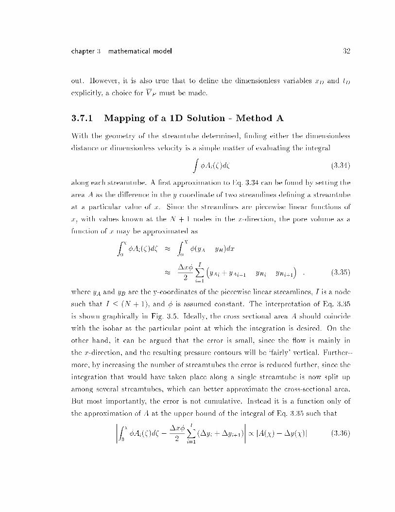
chapter 3 mathematical model 32
out. However, it is also true that to de�ne the dimensionless variables xD and tD
explicitly, a choice for V P must be made.
3.7.1 Mapping of a 1D Solution - Method A
With the geometry of the streamtube determined, �nding either the dimensionless
distance or dimensionless velocity is a simple matter of evaluating the integralZ�Ai(�)d� (3:34)
along each streamtube. A �rst approximation to Eq. 3.34 can be found by setting the
area A as the di�erence in the y coordinate of two streamlines de�ning a streamtube
at a particular value of x. Since the streamlines are piecewise linear functions of
x, with values known at the N + 1 nodes in the x-direction, the pore volume as a
function of x may be approximated asZ�
0
�Ai(�)d� �Z
X
0
�(yA � yB)dx
� �x�
2
IXi=1
�yAi + yAi+1 � yBi
� yBi+1
�: (3.35)
where yA and yB are the y-coordinates of the piecewise linear streamlines, I is a node
such that I � (N + 1), and � is assumed constant. The interpretation of Eq. 3.35
is shown graphically in Fig. 3.5. Ideally, the cross sectional area A should coincide
with the isobar at the particular point at which the integration is desired. On the
other hand, it can be argued that the error is small, since the ow is mainly in
the x-direction, and the resulting pressure contours will be `fairly' vertical. Further-
more, by increasing the number of streamtubes the error is reduced further, since the
integration that would have taken place along a single streamtube is now split up
among several streamtubes, which can better approximate the cross-sectional area.
But most importantly, the error is not cumulative. Instead it is a function only of
the approximation of A at the upper bound of the integral of Eq. 3.35 such that�����Z
�
0
�Ai(�)d� ��x�
2
IXi=1
(�yi +�yi+1)
����� / jA(�)��y(�)j (3:36)
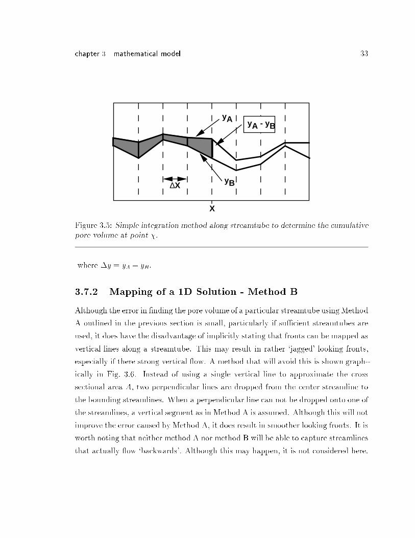
chapter 3 mathematical model 33
yA
yB
yA - yB
∆X
X
Figure 3.5: Simple integration method along streamtube to determine the cumulativepore volume at point �.
where �y = yA � yB.
3.7.2 Mapping of a 1D Solution - Method B
Although the error in �nding the pore volume of a particular streamtube usingMethod
A outlined in the previous section is small, particularly if su�cient streamtubes are
used, it does have the disadvantage of implicitly stating that fronts can be mapped as
vertical lines along a streamtube. This may result in rather `jagged' looking fronts,
especially if there strong vertical ow. A method that will avoid this is shown graph-
ically in Fig. 3.6. Instead of using a single vertical line to approximate the cross
sectional area A, two perpendicular lines are dropped from the center streamline to
the bounding streamlines. When a perpendicular line can not be dropped onto one of
the streamlines, a vertical segment as in Method A is assumed. Although this will not
improve the error caused by Method A, it does result in smoother looking fronts. It is
worth noting that neither method A nor method B will be able to capture streamlines
that actually ow `backwards'. Although this may happen, it is not considered here.
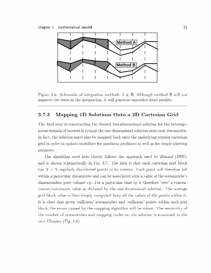
chapter 3 mathematical model 34
AAAAAAMethod A
AAAAAAAAMethod B
Figure 3.6: Schematic of integration methods A & B. Although method B will not
improve the error in the integration, it will generate smoother front pro�les.
3.7.3 Mapping 1D Solutions Onto a 2D Cartesian Grid
The �nal step in constructing the desired two-dimensional solution for the heteroge-
neous domain of interest is to map the one-dimensional solution onto each streamtube.
In fact, the solution must also be mapped back onto the underlying regular cartesian
grid in order to update mobilities for nonlinear problems as well as for simple plotting
purposes.
The algorithm used here closely follows the approach used by Renard (1990),
and is shown schematically in Fig. 3.7. The idea is that each cartesian grid block
has N � N regularly distributed points in its interior. Each point will therefore fall
within a particular streamtube and can be associated with a value of the streamtube's
dimensionless pore volume xD. For a particular time tD it therefore `sees' a concen-
tration/saturation value as dictated by the one-dimensional solution. The average
grid block value is then simply computed from all the values of the points within it.
It is clear that given `su�cient' streamtubes and `su�cient' points within each grid
block, the errors caused by the mapping algorithm will be minor. The sensitivity of
the number of streamtubes and mapping nodes on the solution is examined in the
next Chapter (Fig. 4.6).
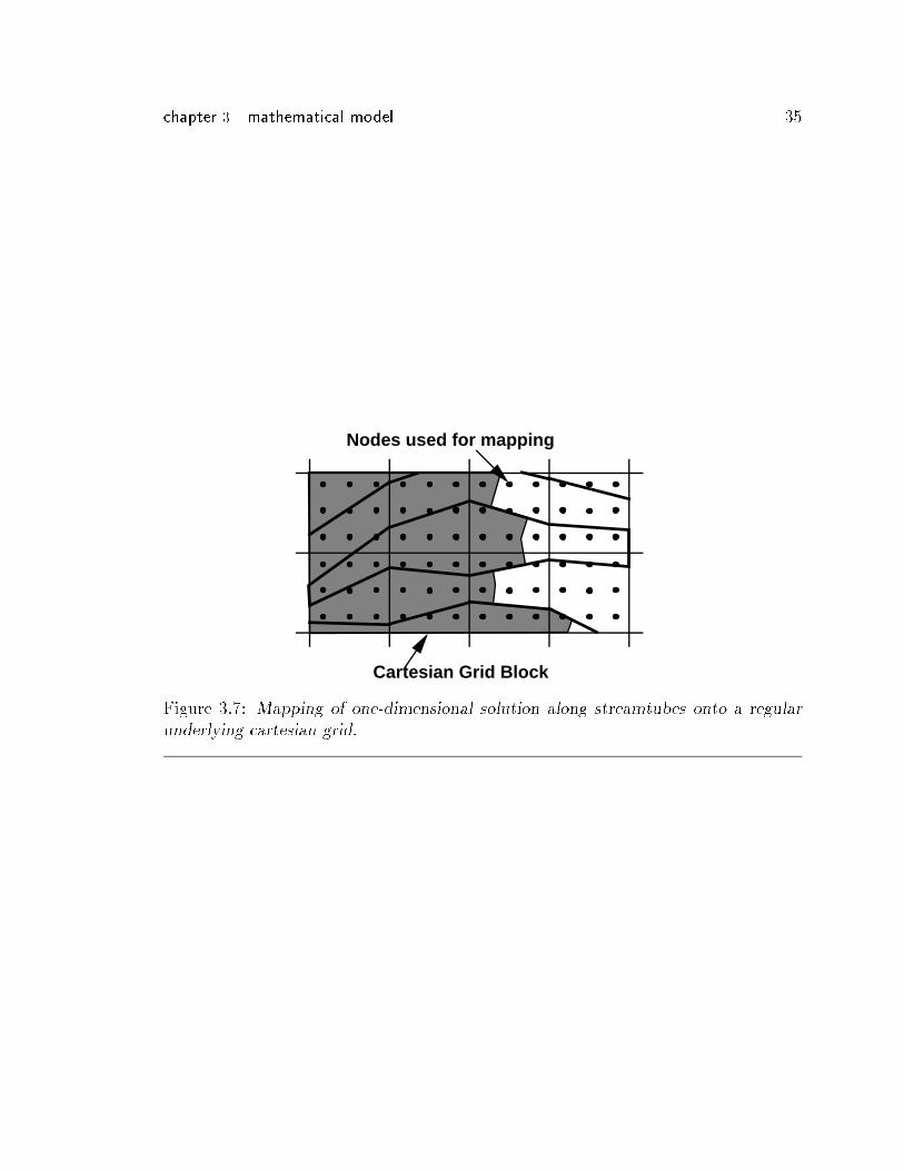
chapter 3 mathematical model 35
Cartesian Grid Block
Nodes used for mapping
Figure 3.7: Mapping of one-dimensional solution along streamtubes onto a regular
underlying cartesian grid.
Chapter 4
Unit Mobility Displacements
This chapter discusses modeling of unit mobility (tracer) displacements using stream-
tubes. Two-dimensional solutions devoid of numerical di�usion are found by map-
ping a one-dimensional, piston-like solution along streamtubes. Longitudinal physical
di�usion is added to the two-dimensional solution by using a convection-di�usion so-
lution along the streamtubes. Under unit mobility assumptions, the two-dimensional
streamtube solution is shown to approach the exact solution in the limit of in�nite
streamtubes.
4.1 Introduction
Unit mobility displacements have been researched extensively in the past. They serve
as a �rst stepping stone to understand the interaction of more complicated, non-
linear multiphase, multicomponent displacements with reservoir heterogeneity. The
numerical advantage of tracer displacements is that the elliptic equation governing
the potential ow �eld is decoupled from the mass conservation equations. The prob-
lem becomes linear in pressure/ ow potential, and the numerically expensive pressure
equation has to be solved only once to model the displacement over any desired time
span, tD. Tracer displacements have found widespread use in two major areas of
petroleum research: to study numerical di�usion and to quantify the e�ects reservoir
heterogeneities (Abbaszadeh-Dehghani 1982, Wattenbarger 1993).
The tracer assumption has also been used extensively in streamtube modeling
36
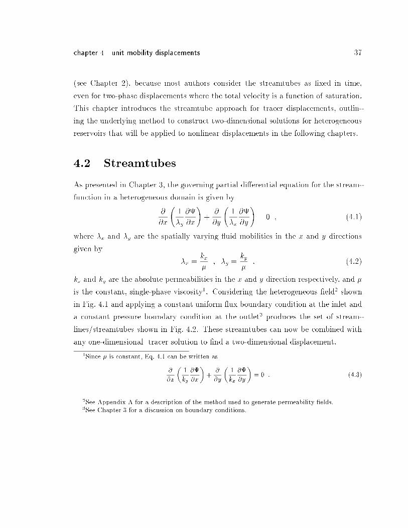
chapter 4 unit mobility displacements 37
(see Chapter 2), because most authors consider the streamtubes as �xed in time,
even for two-phase displacements where the total velocity is a function of saturation.
This chapter introduces the streamtube approach for tracer displacements, outlin-
ing the underlying method to construct two-dimensional solutions for heterogeneous
reservoirs that will be applied to nonlinear displacements in the following chapters.
4.2 Streamtubes
As presented in Chapter 3, the governing partial di�erential equation for the stream-
function in a heterogeneous domain is given by
@
@x
1
�y
@
@x
!+
@
@y
1
�x
@
@y
!= 0 ; (4:1)
where �x and �y are the spatially varying uid mobilities in the x and y directions
given by
�x =kx
�; �y =
ky
�: (4:2)
kx and ky are the absolute permeabilities in the x and y direction respectively, and �
is the constant, single-phase viscosity1. Considering the heterogeneous �eld2 shown
in Fig. 4.1 and applying a constant uniform ux boundary condition at the inlet and
a constant pressure boundary condition at the outlet3 produces the set of stream-
lines/streamtubes shown in Fig. 4.2. These streamtubes can now be combined with
any one-dimensional tracer solution to �nd a two-dimensional displacement.
1Since � is constant, Eq. 4.1 can be written as
@
@x
�1
ky
@
@x
�+
@
@y
�1
kx
@
@y
�= 0 : (4:3)
2See Appendix A for a description of the method used to generate permeability �elds.3See Chapter 3 for a discussion on boundary conditions.
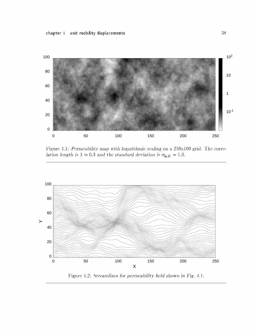
chapter 4 unit mobility displacements 38
0
20
40
60
80
100
0 50 100 150 200 250
10-1
1
10
102
Figure 4.1: Permeability map with logarithmic scaling on a 250x100 grid. The corre-lation length is � � 0:3 and the standard deviation is �lnK = 1:0.
0
20
40
60
80
100
Y
0 50 100 150 200 250X
Figure 4.2: Streamlines for permeability �eld shown in Fig. 4.1.
chapter 4 unit mobility displacements 39
4.3 2D Displacements - No Physical Di�usion
4.3.1 The 1D Solution
The general material balance for the isothermal ow of component i, assuming no
chemical reactions and no adsorption/desorption, is given by (Lake 1989, p.29)
@
@t
0@� NPX
j=1
�jSj!ij
1A +r �
0@NPXj=1
�j!ij~uj � �Sj�j~~Kij � r!ij
1A = 0 ; (4:4)
where
�j = molar density of phase j ,
Sj = saturation of phase j ,
!ij = mole fraction of component i in phase j ,
uj = Darcy velocity of phase j ,
Kij= dispersion of component i in phase j,
Np = number of phases present .
The Darcy velocity for phase j is given by
~uj = �krj
~~k
�j��~rPj + �j~g
�; (4:5)
where
krj = relative permeability of phase j ,
�j = viscosity of phase j ,~~k = absolute permeability tensor ,
P = pressure,
~g = gravity .
Assuming (1) single-phase ow4, (2) horizontal, one-dimensional ow5, (3) no di�usion6,
(4) incompressible uid and rock properties7, (6) ideal mixing8, (7) constant phase
4NP = 1 ; S1 = 1 ; P1 = P ; u1 = u
5~g = 0 ;~~Ki1 = Ki1 ;
~~k = k6Ki1 = 07�1 = � 6= � (P ) ; � 6= �(P )8� =
PNc
i=1 ��
i!i1
chapter 4 unit mobility displacements 40
viscosity9, and (8) homogeneous domain10 the conservation equation for species i
becomes
�@(�wi)
@t+ u
@(�wi)
@x= 0 i = 1; � � � ; Nc : (4:6)
�wi = Ci is the volumetric concentration of component i. Introducing the dimension-
less variables
tD =1
�L
Zt
0
udt =ut
�L(4.7)
xD =x
L(4.8)
CDi =Ci
C�
i
; (4.9)
gives@CDi
@xD+@CDi
@tD= 0 i = 1; � � � ; Nc : (4:10)
Restricting ow to two components only (Nc = 2) gives a single independent conser-
vation equation, where the component subscript is dropped for convenience, as
@CD
@xD+@CD
@tD= 0 : (4:11)
Eq. 4.11 is a linear hyperbolic conservation equation. For constant initial data of the
type
CD(xD; 0)
8<: CDl for xD � 0
CDr for xD � 0; (4:12)
Eq. 4.11 is easily solved by the method of characteristics (Zauderer 1989, LeVeque
1992). The initial data of Eq. 4.12 has a discontinuity at xD = 0. Problems with
this type of initial data are called Riemann problems, where the subscript r refers to
the state to the right of the discontinuity and l refers to the state to the left of the
discontinuity.
9�1 = �10k = constant
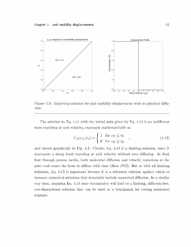
chapter 4 unit mobility displacements 41
0.0
0.2
0.4
0.6
0.8
1.0
Con
cent
ratio
n, C
D
0.0 0.2 0.4 0.6 0.8 1.0 1.2 1.4 1.6 1.8 2.0
Wave Velocity, xD/tD
Concentration Profile
0.0
0.2
0.4
0.6
0.8
1.0
t D
0.0 0.2 0.4 0.6 0.8 1.0xD
tD-xD Diagram for Unit Mobility Displacements
CD = 1.0
CD = 0.0
Figure 4.3: Analytical solution for unit mobility displacement with no physical di�u-sion.
The solution to Eq. 4.11 with the initial data given by Eq. 4.12 is an indi�erent
wave traveling at unit velocity, expressed mathematically as
CD(xD; tD) =
8<: 1 for xD � tD
0 for xD � tD; (4:13)
and shown graphically in Fig. 4.3. Clearly, Eq. 4.13 is a limiting solution, since it
represents a sharp front traveling at unit velocity without ever di�using. In uid
ow through porous media, both molecular di�usion and velocity variations at the
pore scale cause the front to di�use with time (Bear 1972). But as with all limiting
solutions, Eq. 4.13 is important because it is a reference solution against which to
measure numerical solutions that invariably include numerical di�usion. In a similar
way then, mapping Eq. 4.13 onto streamtubes will lead to a limiting, di�usion-free,
two-dimensional solution that can be used as a benchmark for testing numerical
schemes.
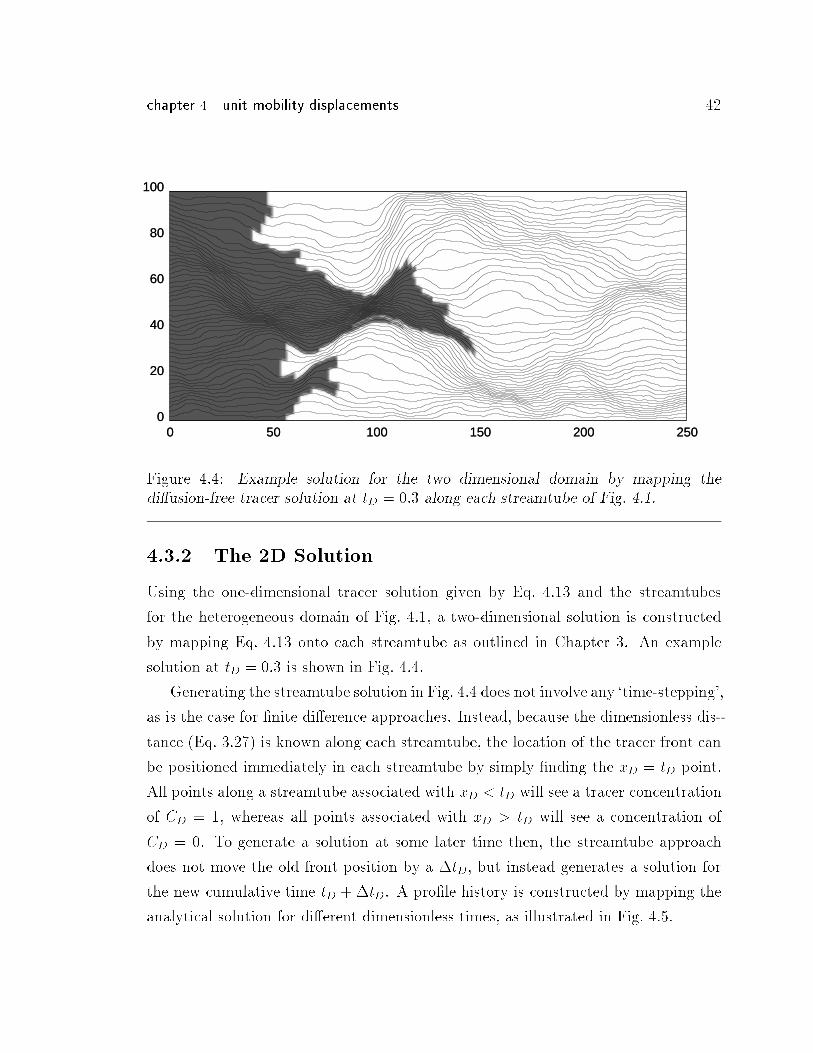
chapter 4 unit mobility displacements 42
0
20
40
60
80
100
0 50 100 150 200 250
0
20
40
60
80
100
0 50 100 150 200 250
Figure 4.4: Example solution for the two dimensional domain by mapping thedi�usion-free tracer solution at tD = 0:3 along each streamtube of Fig. 4.1.
4.3.2 The 2D Solution
Using the one-dimensional tracer solution given by Eq. 4.13 and the streamtubes
for the heterogeneous domain of Fig. 4.1, a two-dimensional solution is constructed
by mapping Eq. 4.13 onto each streamtube as outlined in Chapter 3. An example
solution at tD = 0:3 is shown in Fig. 4.4.
Generating the streamtube solution in Fig. 4.4 does not involve any `time-stepping',
as is the case for �nite di�erence approaches. Instead, because the dimensionless dis-
tance (Eq. 3.27) is known along each streamtube, the location of the tracer front can
be positioned immediately in each streamtube by simply �nding the xD = tD point.
All points along a streamtube associated with xD < tD will see a tracer concentration
of CD = 1, whereas all points associated with xD > tD will see a concentration of
CD = 0. To generate a solution at some later time then, the streamtube approach
does not move the old front position by a �tD, but instead generates a solution for
the new cumulative time tD + �tD. A pro�le history is constructed by mapping the
analytical solution for di�erent dimensionless times, as illustrated in Fig. 4.5.
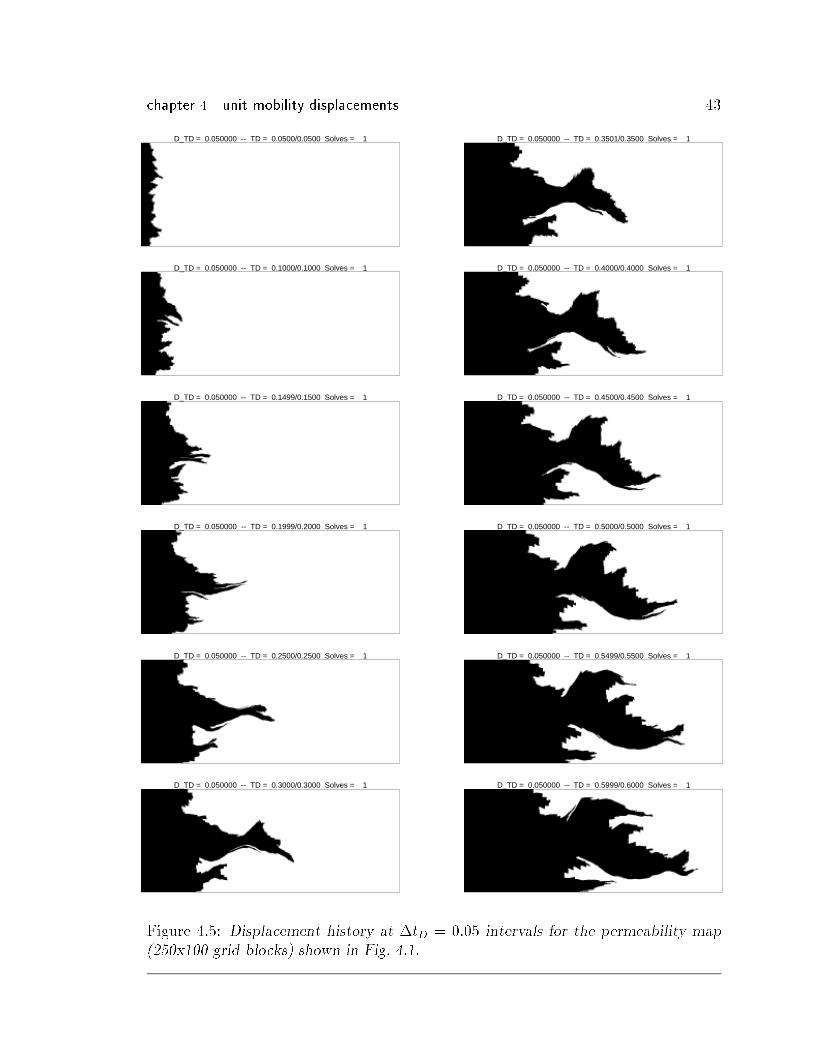
chapter 4 unit mobility displacements 43
D_TD = 0.050000 -- TD = 0.0500/0.0500 Solves = 1
D_TD = 0.050000 -- TD = 0.1000/0.1000 Solves = 1
D_TD = 0.050000 -- TD = 0.1499/0.1500 Solves = 1
D_TD = 0.050000 -- TD = 0.1999/0.2000 Solves = 1
D_TD = 0.050000 -- TD = 0.2500/0.2500 Solves = 1
D_TD = 0.050000 -- TD = 0.3000/0.3000 Solves = 1
D_TD = 0.050000 -- TD = 0.3501/0.3500 Solves = 1
D_TD = 0.050000 -- TD = 0.4000/0.4000 Solves = 1
D_TD = 0.050000 -- TD = 0.4500/0.4500 Solves = 1
D_TD = 0.050000 -- TD = 0.5000/0.5000 Solves = 1
D_TD = 0.050000 -- TD = 0.5499/0.5500 Solves = 1
D_TD = 0.050000 -- TD = 0.5999/0.6000 Solves = 1
Figure 4.5: Displacement history at �tD = 0:05 intervals for the permeability map
(250x100 grid blocks) shown in Fig. 4.1.
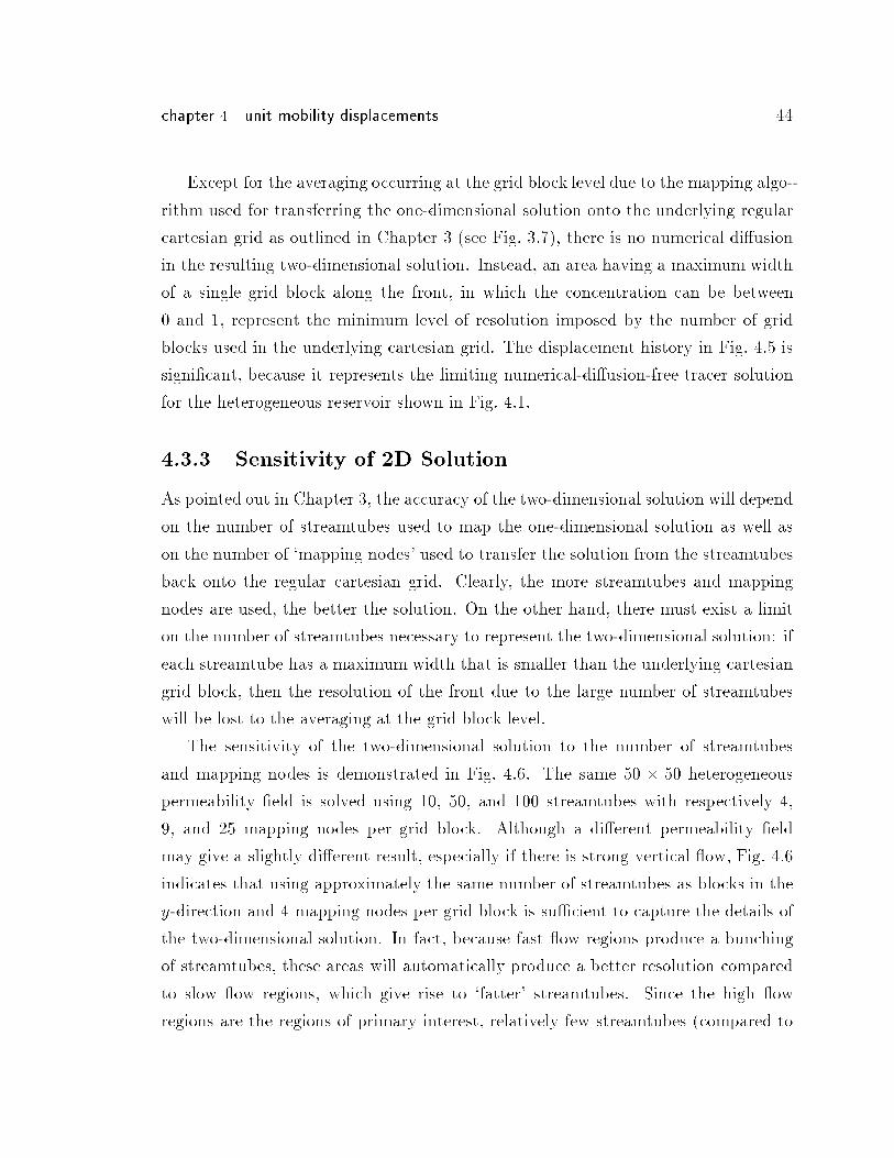
chapter 4 unit mobility displacements 44
Except for the averaging occurring at the grid block level due to the mapping algo-
rithm used for transferring the one-dimensional solution onto the underlying regular
cartesian grid as outlined in Chapter 3 (see Fig. 3.7), there is no numerical di�usion
in the resulting two-dimensional solution. Instead, an area having a maximum width
of a single grid block along the front, in which the concentration can be between
0 and 1, represent the minimum level of resolution imposed by the number of grid
blocks used in the underlying cartesian grid. The displacement history in Fig. 4.5 is
signi�cant, because it represents the limiting numerical-di�usion-free tracer solution
for the heterogeneous reservoir shown in Fig. 4.1.
4.3.3 Sensitivity of 2D Solution
As pointed out in Chapter 3, the accuracy of the two-dimensional solution will depend
on the number of streamtubes used to map the one-dimensional solution as well as
on the number of `mapping nodes' used to transfer the solution from the streamtubes
back onto the regular cartesian grid. Clearly, the more streamtubes and mapping
nodes are used, the better the solution. On the other hand, there must exist a limit
on the number of streamtubes necessary to represent the two-dimensional solution: if
each streamtube has a maximum width that is smaller than the underlying cartesian
grid block, then the resolution of the front due to the large number of streamtubes
will be lost to the averaging at the grid block level.
The sensitivity of the two-dimensional solution to the number of streamtubes
and mapping nodes is demonstrated in Fig. 4.6. The same 50 � 50 heterogeneous
permeability �eld is solved using 10, 50, and 100 streamtubes with respectively 4,
9, and 25 mapping nodes per grid block. Although a di�erent permeability �eld
may give a slightly di�erent result, especially if there is strong vertical ow, Fig. 4.6
indicates that using approximately the same number of streamtubes as blocks in the
y-direction and 4 mapping nodes per grid block is su�cient to capture the details of
the two-dimensional solution. In fact, because fast ow regions produce a bunching
of streamtubes, these areas will automatically produce a better resolution compared
to slow ow regions, which give rise to `fatter' streamtubes. Since the high ow
regions are the regions of primary interest, relatively few streamtubes (compared to
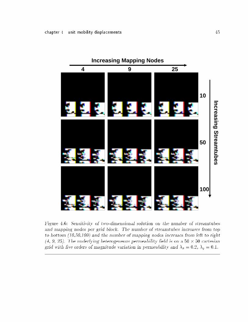
chapter 4 unit mobility displacements 45
Increasing Mapping Nodes
Increasin
g S
treamtu
bes
4 9 25
10
50
100
Figure 4.6: Sensitivity of two-dimensional solution on the number of streamtubesand mapping nodes per grid block. The number of streamtubes increases from top
to bottom (10,50,100) and the number of mapping nodes increases from left to right
(4, 9, 25). The underlying heterogeneous permeability �eld is on a 50 � 50 cartesiangrid with �ve orders of magnitude variation in permeability and �x = 0:2, �y = 0:1.
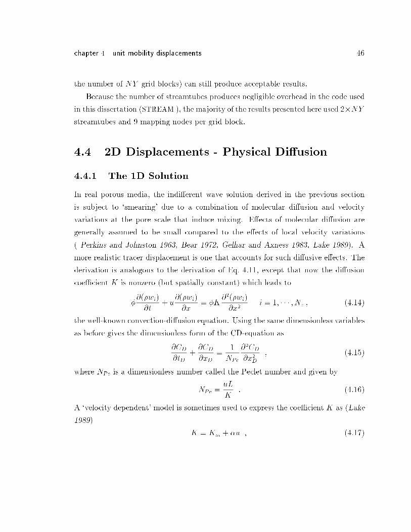
chapter 4 unit mobility displacements 46
the number of NY grid blocks) can still produce acceptable results.
Because the number of streamtubes produces negligible overhead in the code used
in this dissertation (STREAM ), the majority of the results presented here used 2�NY
streamtubes and 9 mapping nodes per grid block.
4.4 2D Displacements - Physical Di�usion
4.4.1 The 1D Solution
In real porous media, the indi�erent wave solution derived in the previous section
is subject to `smearing' due to a combination of molecular di�usion and velocity
variations at the pore scale that induce mixing. E�ects of molecular di�usion are
generally assumed to be small compared to the e�ects of local velocity variations
( Perkins and Johnston 1963, Bear 1972, Gelhar and Axness 1983, Lake 1989). A
more realistic tracer displacement is one that accounts for such di�usive e�ects. The
derivation is analogous to the derivation of Eq. 4.11, except that now the di�usion
coe�cient K is nonzero (but spatially constant) which leads to
�@(�wi)
@t+ u
@(�wi)
@x= �K
@2(�wi)
@x2i = 1; � � � ; Nc ; (4:14)
the well-known convection-di�usion equation. Using the same dimensionless variables
as before gives the dimensionless form of the CD-equation as
@CD
@tD+@CD
@xD=
1
NPe
@2CD
@x2D
; (4:15)
where NPe is a dimensionless number called the Peclet number and given by
NPe =uL
K: (4:16)
A `velocity dependent' model is sometimes used to express the coe�cient K as (Lake
1989)
K = Km + �u ; (4:17)
chapter 4 unit mobility displacements 47
where Km is the molecular di�usion coe�cient and � is the dispersivity of the perme-
able medium11. If the molecular di�usion coe�cient is assumed to be small compared
to the product �u then the Peclet number may be written as
NPe =L
�: (4:18)
Although Eq. 4.18 is very appealing because it gives a `velocity independent' expres-
sion for the Peclet number, it must be used with caution. In general, � is not a
fundamental property of the medium and has been shown to increase with travel dis-
tance in observed �eld data12 (Neuman 1990, Arya et al.1988). On the other hand,
for a completely uncorrelated log-permeability �eld, � is indeed constant and can be
approximated from the covariance of the permeability �eld (Gelhar and Axness 1983,
Dagan 1988). Although Eq. 4.16 and Eq. 4.18 are di�erent, both equations must give
rise to the same constant value of NPe in order to honor the assumption (a spatially
constant coe�cient K) used in deriving the CD-equation.
Eq. 4.15 is now of parabolic form and thus requires an additional boundary condi-
tion compared to its hyperbolic, di�usion-free counterpart. An approximate solution
to Eq. 4.15 using the following initial and boundary conditions (Lake 1989),
CD(xD; tD = 0) = 0 (4.19)
CD(xD = 0; tD) = 1 (4.20)
CD(xD !1; tD) = 0 (4.21)
11The use of the dispersivity � is the reason why the convection-di�usion equation is often referredto as the convection-dispersion equation. In the published literature, di�usion is used to indicatemixing due to molecular di�usion whereas dispersion is used to indicate mixing due to local velocityvariations.
12The fact that � is found to increase with distance traveled in �eld data results from the at-tempt to use a one-dimensional di�usive/dispersive model to capture three-dimensional, convectivedominated ow. E�ects due to heterogeneities across various scales are lumped into a single pa-rameter, leading to a dependence of � on distance traveled. In the streamtube method, however, atleast two heterogeneity scales are being separated explicitly: �eld scale heterogeneities are de�nedby the streamtube geometries, while sub-streamtube heterogeneities may be captured using �. SeeSection 4.4.2 for a discussion on the subject.
chapter 4 unit mobility displacements 48
0.0
0.2
0.4
0.6
0.8
1.0
Con
cent
ratio
n/S
atur
atio
n
0.0 0.2 0.4 0.6 0.8 1.0Dimensionless Porevolume, XD
NPe = infinityNPe = 1000NPe = 100
Figure 4.7: One-dimensional analytical solutions for the convection-di�usion equationat tD = 0:3 and three values of NPe.
is given by13
CD(xD; tD) =1
2erfc
0@xD � tD
2q
tD
NPe
1A : (4:22)
Adding physical di�usion to a two-dimensional displacements therefore amounts to
mapping Eq. (4.22) onto each streamtube for a given value of NPe. Example solutions
at tD = 0:3 and three values of NPe are shown in Fig. 4.7.
4.4.2 The 2D Solution
Mapping Eq. 4.22 onto streamtubes is slightly di�erent from mapping the no-di�usion
solution, since Eq. 4.22 is clearly not scalable by xD=tD. To �nd the solution for a
particular time tD, Eq. 4.22 must be evaluated explicitly for that time. Nevertheless,
it is important to realize that as in the no-di�usion case, there is no time-stepping
13The exact solution is
CD(xD; tD) =1
2erfc
0@xD � tD
2q
tDNPe
1A+
1
2exDNPeerfc
0@xD + tD
2q
tDNPe
1A ;
but the second term goes to zero exponentially as tD, xD, and NPe grow.
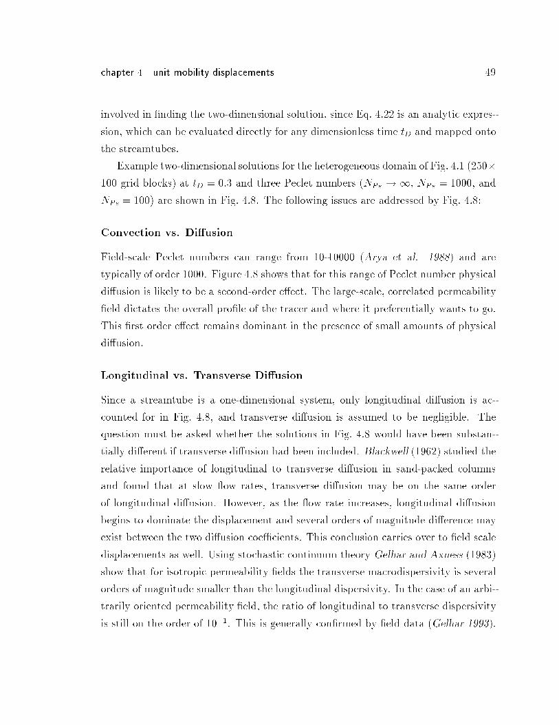
chapter 4 unit mobility displacements 49
involved in �nding the two-dimensional solution, since Eq. 4.22 is an analytic expres-
sion, which can be evaluated directly for any dimensionless time tD and mapped onto
the streamtubes.
Example two-dimensional solutions for the heterogeneous domain of Fig. 4.1 (250�100 grid blocks) at tD = 0:3 and three Peclet numbers (NPe !1, NPe = 1000, and
NPe = 100) are shown in Fig. 4.8. The following issues are addressed by Fig. 4.8:
Convection vs. Di�usion
Field-scale Peclet numbers can range from 10-10000 (Arya et al. 1988) and are
typically of order 1000. Figure 4.8 shows that for this range of Peclet number physical
di�usion is likely to be a second-order e�ect. The large-scale, correlated permeability
�eld dictates the overall pro�le of the tracer and where it preferentially wants to go.
This �rst order e�ect remains dominant in the presence of small amounts of physical
di�usion.
Longitudinal vs. Transverse Di�usion
Since a streamtube is a one-dimensional system, only longitudinal di�usion is ac-
counted for in Fig. 4.8, and transverse di�usion is assumed to be negligible. The
question must be asked whether the solutions in Fig. 4.8 would have been substan-
tially di�erent if transverse di�usion had been included. Blackwell (1962) studied the
relative importance of longitudinal to transverse di�usion in sand-packed columns
and found that at slow ow rates, transverse di�usion may be on the same order
of longitudinal di�usion. However, as the ow rate increases, longitudinal di�usion
begins to dominate the displacement and several orders of magnitude di�erence may
exist between the two di�usion coe�cients. This conclusion carries over to �eld scale
displacements as well. Using stochastic continuum theory Gelhar and Axness (1983)
show that for isotropic permeability �elds the transverse macrodispersivity is several
orders of magnitude smaller than the longitudinal dispersivity. In the case of an arbi-
trarily oriented permeability �eld, the ratio of longitudinal to transverse dispersivity
is still on the order of 10�1. This is generally con�rmed by �eld data (Gelhar 1993).
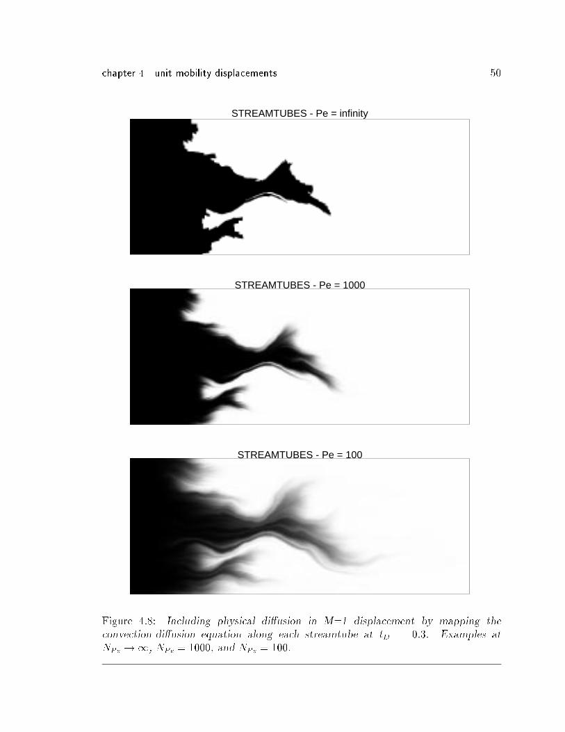
chapter 4 unit mobility displacements 50
STREAMTUBES - Pe = infinity
STREAMTUBES - Pe = 1000
STREAMTUBES - Pe = 100
Figure 4.8: Including physical di�usion in M=1 displacement by mapping the
convection-di�usion equation along each streamtube at tD = 0:3. Examples at
NPe !1, NPe = 1000, and NPe = 100.
chapter 4 unit mobility displacements 51
Thus, it is fair to say that if the solutions in Fig. 4.8 are assumed on a �eld scale,
transverse di�usion would not change them signi�cantly.
Scale of the 2D Solution
Mapping a convection-di�usion solution onto the streamtubes automatically attaches
a length scale to the system. The asymptotic behavior of the longitudinal dispersivity
through a low variance, second-order stationary, permeability �eld may be expressed
as (Gelhar and Axness 1983, Dagan 1988, Neumann 1990)
� =Z1
0
C(h)dh �ZLrep
0
C(h)dh � B�2Lrep (4:23)
where Lrep is a representative length scale beyond which the system looks `di�usive'
(or Fickian), C(h) is the covariance as a function of separation length h, and B is a
constant. For example, if the C(h) is linear between 0 and Lrep then B = 0:5 and
using Eq. 4.23, the Peclet number can be expressed as
NPe =2
�2L
Lrep
: (4:24)
By choosing a Peclet number then, a representative length scale (Lrep) is automatically
introduced beyond which the systems is said to be di�usive. What order of magnitude
Lrep can have though, is a matter of heated debate. If the porous medium is modeled
as a series of well{stirred `tanks' (Aris and Amundson 1957), then in the limit of a
large number of pores a Fickian di�usion model is indeed valid. In this case, Lrep
is on the order of the representative element volume (REV) used in the continuum
approach to porous media. Laboratory displacements through `homogeneous' cores
have generally con�rmed this (Brigham et al. 1961, Blackwell 1962). If Lrep is on the
order of the REV, then the two{dimensional streamtube scale could be several orders
of magnitude larger, maybe on a O(1m) or possibly even O(10m) scale.
For �eld scales, however, there exists considerable uncertainty what Lrep should
be, or even if a such number has a meaning at all. Ample experimental data from
�eld tracer tests demonstrate convincingly the inadequacy of the convection{di�usion
model in matching the integrated concentration response at the production wells
(Arya et al. 1988). Nevertheless, considerable e�ort has gone into showing under
chapter 4 unit mobility displacements 52
what conditions the convection{di�usion equation may be applicable to �eld scale
displacements and when not (Matheron and de Marsily 1980, Gelhar and Axeness
1983, Dagan 1983;1984;1988, Arya et al. 1988, Neumann 1990). Numerical exper-
iments (Smith and Schwartz 1980, Desbartes 1990, Wattenbarger 1993) have also
shown that a di�usive limit is reached only for Lrep << �c << L and �2ln k small,
where Lrep is the di�usive length scale at the pore level, �c is the correlation length
scale of the permeability �eld, and L is the domain dimension in the main direction
of ow. Others (Waggoner et al. 1992), on the other hand, have reported relatively
large `dispersive' regions in �{�2ln k parameter space.
The real question in applying in the CD{model to �eld{scale streamtubes though,
is whether a sub{�eld scale Lrep exists that allows the CD{solution to hold along
�eld{scale streamtubes. A numerical example of this idea is given by Wattenbarger
(1993) In essence, the idea is that each streamtube can be treated as a system having
the necessary characteristics (Lrep << �c << L and �2ln k small) so as to allow a Fick-
ian limit to be reached within each streamtube. Considering that the streamtubes, by
de�nition, will conform to the ow units (heterogeneity) of the system, the assumption
of treating each streamtube as a pseudo homogeneous unit that reaches a di�usive
limit is not unreasonable. In other words, a small Lrep does not necessarily preclude
the streamtubes to be on a �eld scale. For example, successful matching of �eld tracer
data using this approach has been demonstrated by Abbaszadeh{Dehghani (1982).
In summary, mapping the CD-model along �eld-scale streamtubes is an attempt to
capture sub-tube heterogeneities, which are represented numerically by specifying an
appropriate Peclet number. It represents a `nested' approach to modeling hetero-
geneities that dominate at di�erent scales: the streamtubes capture the large-scale
heterogeneities of the reservoir while the CD-solution models sub-grid block/sub-
streamtube features.
Limiting Two-Dimensional Solution
The NPe !1 solution is the limiting no-di�usion solution and serves as the reference
point to quantify any di�usive behavior. The no-di�usion solution is an important
ingredient in quantifying numerical di�usion, as will be discussed in the next section.
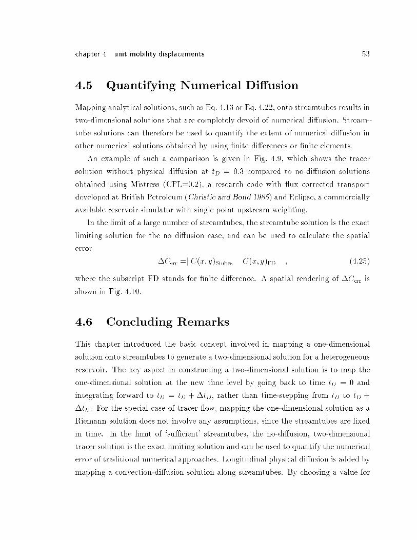
chapter 4 unit mobility displacements 53
4.5 Quantifying Numerical Di�usion
Mapping analytical solutions, such as Eq. 4.13 or Eq. 4.22, onto streamtubes results in
two-dimensional solutions that are completely devoid of numerical di�usion. Stream-
tube solutions can therefore be used to quantify the extent of numerical di�usion in
other numerical solutions obtained by using �nite di�erences or �nite elements.
An example of such a comparison is given in Fig. 4.9, which shows the tracer
solution without physical di�usion at tD = 0:3 compared to no-di�usion solutions
obtained using Mistress (CFL=0.2), a research code with ux corrected transport
developed at British Petroleum (Christie and Bond 1985) and Eclipse, a commercially
available reservoir simulator with single point upstream weighting.
In the limit of a large number of streamtubes, the streamtube solution is the exact
limiting solution for the no di�usion case, and can be used to calculate the spatial
error
�Cerr =j C(x; y)Stubes � C(x; y)FD j ; (4:25)
where the subscript FD stands for �nite di�erence. A spatial rendering of �Cerr is
shown in Fig. 4.10.
4.6 Concluding Remarks
This chapter introduced the basic concept involved in mapping a one-dimensional
solution onto streamtubes to generate a two-dimensional solution for a heterogeneous
reservoir. The key aspect in constructing a two-dimensional solution is to map the
one-dimensional solution at the new time level by going back to time tD = 0 and
integrating forward to tD = tD + �tD, rather than time-stepping from tD to tD +
�tD. For the special case of tracer ow, mapping the one-dimensional solution as a
Riemann solution does not involve any assumptions, since the streamtubes are �xed
in time. In the limit of `su�cient' streamtubes, the no-di�usion, two-dimensional
tracer solution is the exact limiting solution and can be used to quantify the numerical
error of traditional numerical approaches. Longitudinal physical di�usion is added by
mapping a convection-di�usion solution along streamtubes. By choosing a value for
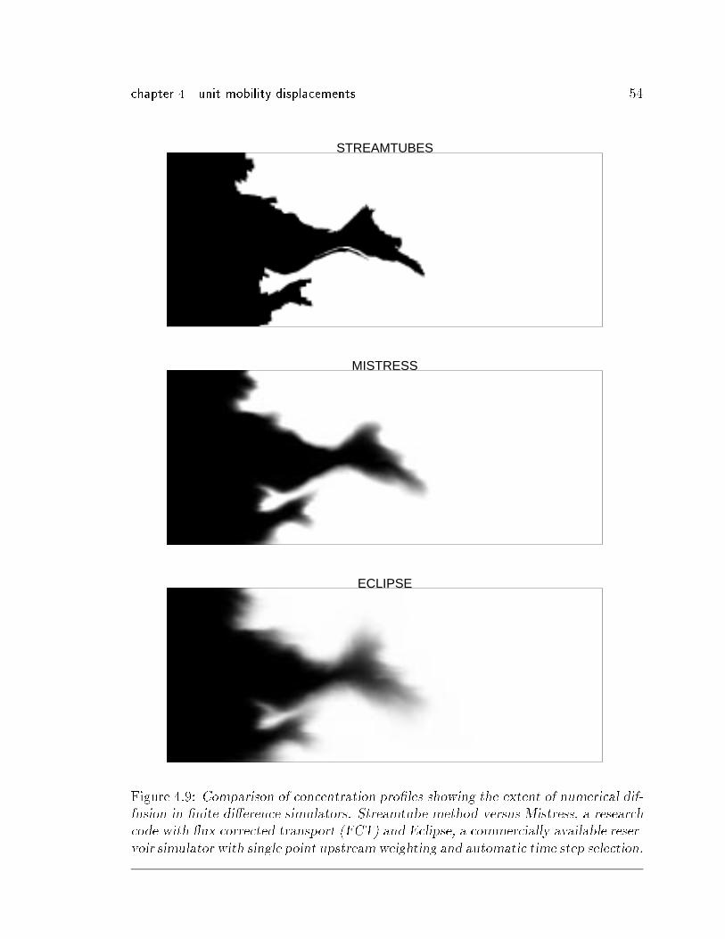
chapter 4 unit mobility displacements 54
STREAMTUBES
MISTRESS
ECLIPSE
Figure 4.9: Comparison of concentration pro�les showing the extent of numerical dif-
fusion in �nite di�erence simulators. Streamtube method versus Mistress, a research
code with ux corrected transport (FCT) and Eclipse, a commercially available reser-
voir simulator with single point upstream weighting and automatic time step selection.
chapter 4 unit mobility displacements 55
Error - Mistress
Error - Eclipse
0.0
0.2
0.4
0.6
0.8
1.0
Figure 4.10: Spatial distribution of the error caused by numerical di�usion in theMistress and Eclipse simulations shown in Fig. 4.9.
the Peclet number in the convection-di�usion model, an implicit assumption about
the scale of the two-dimensional solutions is made. In particular, sub-streamtube
heterogeneities are assumed to lead to a Fickian limit. Thus, the streamtube approach
is an example of how physical phenomena that take place at di�erent scales can be
nested into a single model: the geometries of the streamtube explicitly model large
scale heterogeneities that give rise to fast and slow ow regions, while the convection-
di�usion solution implicitly models sub-streamtube heterogeneities that cause local
mixing.
Chapter 5
Immiscible Displacements
This chapter discusses modeling of two-phase, immiscible displacements using stream-
tubes. The concept of mapping one{dimensional Riemann solutions along stream-
tubes is developed further, and the resulting two{dimensional solutions are shown to
match solutions obtained using a conventional �nite di�erence approach.The immisci-
ble problem is found to be only weakly nonlinear resulting in converged solutions using
two orders of magnitude fewer matrix inversions than in traditional �nite di�erence
simulation. The speed of the streamtube approach is used to study the interaction of
nonlinearity and reservoir heterogeneity in immiscible displacements, demonstrating
an increasing uncertainty in recovery with increasing reservoir heterogeneity.
5.1 Introduction
When Higgins and Leighton (1962) introduced the streamtube approach as a fast
method to predict two{phase ow in a �ve{spot pattern, they reported excellent
agreement with experimental data for mobility ratios ranging from 0:083 to 754.
Other authors (Higgins et al. 1964, Doyle and Wurl 1971, LeBlanc and Caudle 1971,
Martin and Wegner 1979) also reported good matches with either �eld or labora-
tory data for similar values of mobility ratios. All authors were able to account for
the nonlinearity inherent in the total velocity �eld by keeping the streamtubes �xed
and adjusting the owrates instead. The only published note on the failure of the
streamtube approach is by Martin et al. (1973) and, surprisingly, it is for a favorable
56
chapter 5 immiscible displacements 57
mobility ratio case. Intuitively, high unfavorable mobility ratio displacements are
expected to have a `stronger' nonlinearity and thus be more di�cult to model nu-
merically, whereas the favorable mobility ratio displacements are by de�nition stable.
The answer is that while the end{point mobility ratios reported by many authors
are very high, the resulting 1D solutions exhibit a very long rarefaction wave lead-
ing to smooth changes in the velocity �elds. Favorable mobility ratios, on the other
hand, have self-sharpening shocks, across which properties vary abruptly leading to
much sharper changes in the velocity �elds. Two{phase immiscible displacements
with unfavorable mobility ratios and reasonable rock curves will therefore either have
shock{front mobility ratios close to 1 or just long rarefaction waves.
It is this weak nonlinearity in the velocity �eld that allows for the assump-
tion of constant streamtube geometries, which are almost universally applied in the
petroleum literature1. The assumption of �xed streamtubes is also reinforced by the
areal geometry used by all authors since, by continuity, a streamline must start and
end at a source point, leaving little room for the streamtubes to change their shape
during the displacement. Adjusting the ow rates for each streamtube according to
the total resistance of the system is su�cient to capture the nonlinear allocation of
uids that would result from changing streamtubes. Although the approaches dif-
fer slightly from author to author, all show convincingly that constant streamtubes
can successfully and inexpensively predict recovery for most two-dimensional, areal
water ood problems.
5.1.1 The Riemann Approach
In this chapter, the water ood problem is approached di�erently and used principally
to demonstrate the applicability of the Riemann approach proposed in this work and
to be used for multiphase, multicomponent displacements in later chapters. As in
the tracer case, the domain is considered to be heterogeneous and the geometry to
be cross-sectional. Compared to the areal domain, the streamlines are now no longer
pinned down by two (or more) singularities, making them `freer' to move and to re ect
1A notable exception is Renard (1990)
chapter 5 immiscible displacements 58
the nonlinearity in the ow �eld.
The principal di�erence to work done by previous authors lies is in the mapping
of the one-dimensional solution along streamtubes which are periodically updated to
model the nonlinearity of the displacement. In the Riemann approach used here, the
one-dimensional solution is treated as a solution to a Riemann problem, although the
streamtubes are updated periodically. Thus, the solution along a new streamtube
for the time level tD + �tD is not given by an integration from tD to tD + �tD,
as in conventional time-stepping algorithms, but rather as an integration from 0 to
tD+�tD, where the initial conditions are assumed to be constant right and left states.
The Riemann approach centers on treating each periodically updated streamtube as
a true one-dimensional system on which the Buckley-Leverett solution is mapped
repeatedly for di�erent times. The underlying assumption in the Riemann approach
is that the uid entering a streamtube remains in the streamtube and exits only at
the outlet end, even if the streamtube changes location and geometry as a function
of time. The validity of this approach is considered in the sections that follow.
5.1.2 Reasons for the Riemann Approach
A legitimate question is to ask what motivates the Riemann approach. The answer
centers on the attempt to capture the nonlinearities that exist in multiphase ow.
Only three authors (Martin et al. 1973, Martin and Wegner 1979, Renard 1990)
address the idea of updating the streamtubes, rather than using total ow resistance
to capture the nonlinear behavior of the displacement. Mathematically, updating the
streamtubes is an appealing approach because the local ow velocities are updated,
and the original de�nition of a streamtube as carrying a volumetric rate equal to the
di�erence in the value of its bounding streamlines is maintained. However, updating
the streamtubes poses one problem related to the initial conditions associated with
each streamtube: each time a streamtube is updated it must be initialized so that the
conservation equation(s) can be solved. The only reasonable possibility to assign new
initial conditions along an updated streamtube is to use the old, two{dimensional sat-
uration distribution on the underlying cartesian grid. Because updating a streamtube
literally means changing its position in x{y space, it is easy to see that the new initial
chapter 5 immiscible displacements 59
conditions will not correspond to the old saturation distribution along the stream-
tube. The resulting hyperbolic problem that must be solved will be one with general,
nonconstant initial conditions. No analytical solutions exist for such problems and
the saturation distribution along the new streamtube can be moved forward in time
either (1) numerically by using a standard one{dimensional �nite{di�erence solution
along each streamtube (Bommer and Schechter 1979), or (2) by using a moving in-
terface, front{tracking algorithm (Sheldon and Dougherty 1964, Glimm et al. 1983,
Bratvedt et al. 1989). The Riemann approach, on the other hand, completely cir-
cumvents the problem of initial conditions that arises with streamtube updating: the
two{dimensional solution is approximated by N one{dimensional Riemann solutions
along changing streamtubes.
5.2 The 1D Buckley{Leverett Solution
The one-dimensional Buckley{Leverett solution is well known and well documented in
the petroleum literature (Buckley and Leverett 1941, Dake 1978, Lake 1989). Starting
from the general material balance for component i (Lake 1989, p.29)
@
@t
0@� NPX
j=1
�jSj!ij
1A +r �
0@NPXj=1
�j!ij~uj � �Sj�j~~Kij � r!ij
1A = 0 ; (5:1)
and assuming (1) two component, two{phase, immiscible ow2, (2) no di�usion3,
(3) constant and equal phase densities4, and (4) one{dimensional ow gives the well
known equation
�@Sw
@t+@uw
@x= 0 ; (5:2)
where the subscript for component i = 1 has been replaced with w, to keep with
the traditional application to oil{water systems. Eq. 5.2 is generally used in its
dimensionless form@Sw
@tD+@fw
@xD= 0 ; (5:3)
2!11 = !22 = 1; !12 = !21 = 0
3 ~~Kij = 04�1 = �2
chapter 5 immiscible displacements 60
where tD = tut=L and xD = �x=L are usual de�nitions of dimensionless time and
distance respectively, ut is the total (constant) Darcy velocity given by ut = uw + uo,
and fw is the fractional ow of water given by
fw =uw
uw + uo=
1
1 + kro�w
krw�o
: (5:4)
kro, krw, �o, and �w are the relative permeabilities and viscosities of oil and water as
indicated by the subscript5. The solution to Eq. 5.3 subject to Riemann conditions
of the form
Sw(xD; 0)
8<: Swl for xD � 0
Swr for xD � 0; (5:5)
where, as in the tracer case (Eq. 4.12), the subscripts l and r refer to the left and
right constant states of the discontinuity at xD = 0, can be found easily using the
method of characteristics (Zauderer 1989, LeVeque 1992). Depending on the shape of
the fractional ow curve, fw, the solution can contain rarefaction waves and shocks,
which are found using the velocity constraint and the entropy condition (Johns 1992).
A rarefaction wave is composed of saturations having characteristic velocities given
bydxD
dtD=
dfw
dSw; (5:6)
whereas a shock travels with a characteristic velocity given by
dxD
dtD=
fUw� fD
w
SUw� SD
w
: (5:7)
The superscripts U and D stand for upstream and downstream respectively. An
example solution for a two{phase problem with an end{point mobility ratio of 10 is
shown in Fig. 5.1.
5.3 Validation of the Riemann Approach
The Riemann approach was tested by the following numerical experiment. Using
a standard �nite di�erence simulator (Eclipse), the velocity �elds were stored for
5Eq. 5.4 assumes that the one{dimensional reservoir is homogeneous.
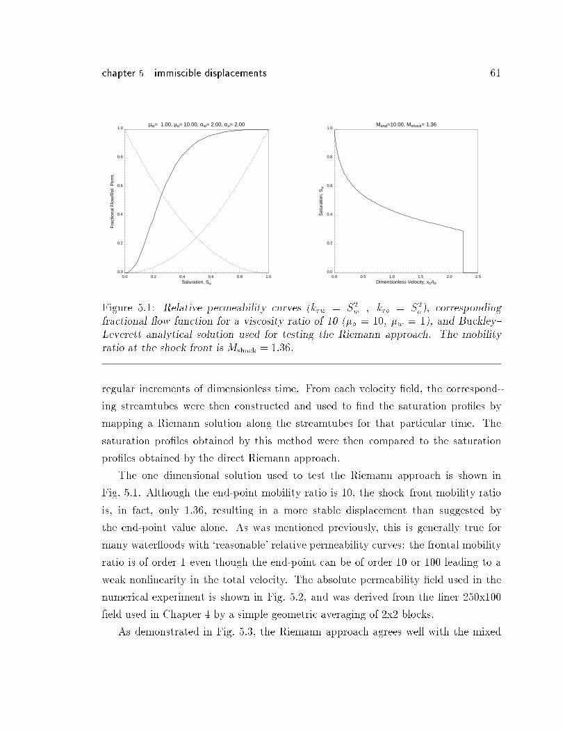
chapter 5 immiscible displacements 61
0.0
0.2
0.4
0.6
0.8
1.0
Sat
urat
ion,
Sw
0.0 0.5 1.0 1.5 2.0 2.5Dimensionless Velocity, xD/tD
Mend=10.00, Mshock= 1.36
0.0
0.2
0.4
0.6
0.8
1.0
Fra
ctio
nal F
low
/Rel
. Per
m.
0.0 0.2 0.4 0.6 0.8 1.0Saturation, Sw
µw= 1.00, µo= 10.00, αw= 2.00, αo= 2.00
Figure 5.1: Relative permeability curves (krw = S2w; kro = S2
o), corresponding
fractional ow function for a viscosity ratio of 10 (�o = 10, �w = 1), and Buckley{Leverett analytical solution used for testing the Riemann approach. The mobilityratio at the shock front is Mshock = 1:36.
regular increments of dimensionless time. From each velocity �eld, the correspond-
ing streamtubes were then constructed and used to �nd the saturation pro�les by
mapping a Riemann solution along the streamtubes for that particular time. The
saturation pro�les obtained by this method were then compared to the saturation
pro�les obtained by the direct Riemann approach.
The one{dimensional solution used to test the Riemann approach is shown in
Fig. 5.1. Although the end-point mobility ratio is 10, the shock{front mobility ratio
is, in fact, only 1.36, resulting in a more stable displacement than suggested by
the end-point value alone. As was mentioned previously, this is generally true for
many water oods with `reasonable' relative permeability curves: the frontal mobility
ratio is of order 1 even though the end-point can be of order 10 or 100 leading to a
weak nonlinearity in the total velocity. The absolute permeability �eld used in the
numerical experiment is shown in Fig. 5.2, and was derived from the �ner 250x100
�eld used in Chapter 4 by a simple geometric averaging of 2x2 blocks.
As demonstrated in Fig. 5.3, the Riemann approach agrees well with the mixed
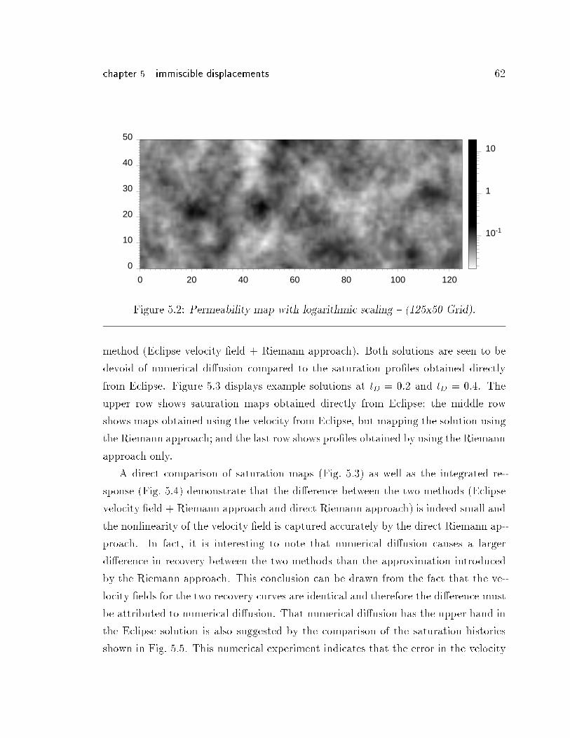
chapter 5 immiscible displacements 62
0
10
20
30
40
50
0 20 40 60 80 100 120
10-1
1
10
Figure 5.2: Permeability map with logarithmic scaling { (125x50 Grid).
method (Eclipse velocity �eld + Riemann approach). Both solutions are seen to be
devoid of numerical di�usion compared to the saturation pro�les obtained directly
from Eclipse. Figure 5.3 displays example solutions at tD = 0:2 and tD = 0:4. The
upper row shows saturation maps obtained directly from Eclipse; the middle row
shows maps obtained using the velocity from Eclipse, but mapping the solution using
the Riemann approach; and the last row shows pro�les obtained by using the Riemann
approach only.
A direct comparison of saturation maps (Fig. 5.3) as well as the integrated re-
sponse (Fig. 5.4) demonstrate that the di�erence between the two methods (Eclipse
velocity �eld + Riemann approach and direct Riemann approach) is indeed small and
the nonlinearity of the velocity �eld is captured accurately by the direct Riemann ap-
proach. In fact, it is interesting to note that numerical di�usion causes a larger
di�erence in recovery between the two methods than the approximation introduced
by the Riemann approach. This conclusion can be drawn from the fact that the ve-
locity �elds for the two recovery curves are identical and therefore the di�erence must
be attributed to numerical di�usion. That numerical di�usion has the upper hand in
the Eclipse solution is also suggested by the comparison of the saturation histories
shown in Fig. 5.5. This numerical experiment indicates that the error in the velocity
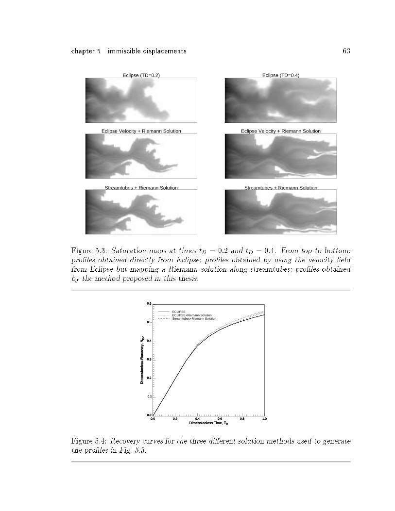
chapter 5 immiscible displacements 63
Streamtubes + Riemann Solution
Eclipse Velocity + Riemann Solution
Eclipse (TD=0.2)
Streamtubes + Riemann Solution
Eclipse Velocity + Riemann Solution
Eclipse (TD=0.4)
Figure 5.3: Saturation maps at times tD = 0:2 and tD = 0:4. From top to bottom:pro�les obtained directly from Eclipse; pro�les obtained by using the velocity �eldfrom Eclipse but mapping a Riemann solution along streamtubes; pro�les obtainedby the method proposed in this thesis.
0.0
0.1
0.2
0.3
0.4
0.5
0.6
Dim
ensi
onle
ss R
ecov
ery,
NpD
0.0 0.2 0.4 0.6 0.8 1.0Dimensionless Time, TD
0.0
0.1
0.2
0.3
0.4
0.5
0.6
Dim
ensi
onle
ss R
ecov
ery,
NpD
0.0 0.2 0.4 0.6 0.8 1.0Dimensionless Time, TD
0.0
0.1
0.2
0.3
0.4
0.5
0.6
Dim
ensi
onle
ss R
ecov
ery,
NpD
0.0 0.2 0.4 0.6 0.8 1.0Dimensionless Time, TD
ECLIPSEECLIPSE+Riemann SolutionStreamtubes+Riemann Solution
Figure 5.4: Recovery curves for the three di�erent solution methods used to generate
the pro�les in Fig. 5.3.
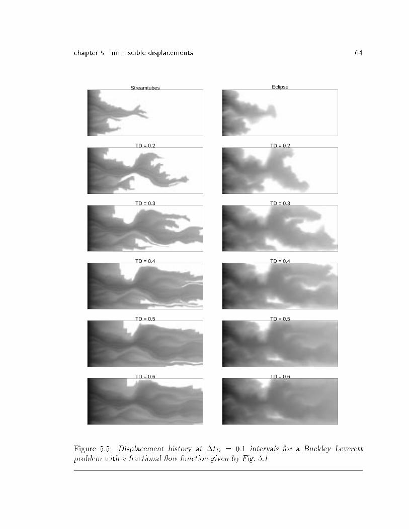
chapter 5 immiscible displacements 64
Streamtubes
TD = 0.2
TD = 0.3
TD = 0.4
TD = 0.5
TD = 0.6
Eclipse
TD = 0.2
TD = 0.3
TD = 0.4
TD = 0.5
TD = 0.6
Figure 5.5: Displacement history at �tD = 0:1 intervals for a Buckley{Leverett
problem with a fractional ow function given by Fig. 5.1
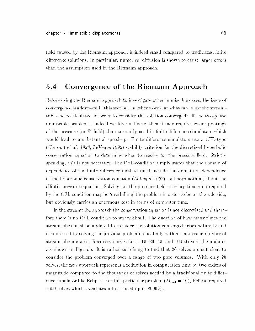
chapter 5 immiscible displacements 65
�eld caused by the Riemann approach is indeed small compared to traditional �nite
di�erence solutions. In particular, numerical di�usion is shown to cause larger errors
than the assumption used in the Riemann approach.
5.4 Convergence of the Riemann Approach
Before using the Riemann approach to investigate other immiscible cases, the issue of
convergence is addressed in this section. In other words, at what rate must the stream-
tubes be recalculated in order to consider the solution converged? If the two-phase
immiscible problem is indeed weakly nonlinear, then it may require fewer updatings
of the pressure (or {�eld) than currently used in �nite di�erence simulators which
would lead to a substantial speed-up. Finite di�erence simulators use a CFL-type
(Courant et al. 1928, LeVeque 1992) stability criterion for the discretized hyperbolic
conservation equation to determine when to resolve for the pressure �eld. Strictly
speaking, this is not necessary. The CFL-condition simply states that the domain of
dependence of the �nite di�erence method must include the domain of dependence
of the hyperbolic conservation equation (LeVeque 1992), but says nothing about the
elliptic pressure equation. Solving for the pressure �eld at every time step required
by the CFL condition may be `overkilling' the problem in order to be on the safe side,
but obviously carries an enormous cost in terms of computer time.
In the streamtube approach the conservation equation is not discretized and there-
fore there is no CFL condition to worry about. The question of how many times the
streamtubes must be updated to consider the solution converged arises naturally and
is addressed by solving the previous problem repeatedly with an increasing number of
streamtube updates. Recovery curves for 1, 10, 20, 40, and 100 streamtube updates
are shown in Fig. 5.6. It is rather surprising to �nd that 20 solves are su�cient to
consider the problem converged over a range of two pore volumes. With only 20
solves, the new approach represents a reduction in computation time by two orders of
magnitude compared to the thousands of solves needed by a traditional �nite di�er-
ence simulator like Eclipse. For this particular problem (Mend = 10), Eclipse required
1600 solves which translates into a speed-up of 8000% .
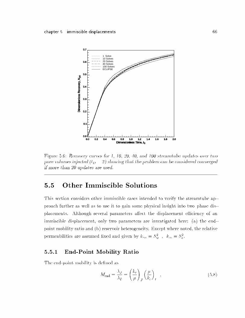
chapter 5 immiscible displacements 66
0.0
0.1
0.2
0.3
0.4
0.5
0.6
0.7
Dim
ensi
onle
ss R
ecov
ery,
NpD
0.0 0.2 0.4 0.6 0.8 1.0 1.2 1.4 1.6 1.8 2.0Dimensionless Time, tD
0.0
0.1
0.2
0.3
0.4
0.5
0.6
0.7
Dim
ensi
onle
ss R
ecov
ery,
NpD
0.0 0.2 0.4 0.6 0.8 1.0 1.2 1.4 1.6 1.8 2.0Dimensionless Time, tD
0.0
0.1
0.2
0.3
0.4
0.5
0.6
0.7
Dim
ensi
onle
ss R
ecov
ery,
NpD
0.0 0.2 0.4 0.6 0.8 1.0 1.2 1.4 1.6 1.8 2.0Dimensionless Time, tD
0.0
0.1
0.2
0.3
0.4
0.5
0.6
0.7
Dim
ensi
onle
ss R
ecov
ery,
NpD
0.0 0.2 0.4 0.6 0.8 1.0 1.2 1.4 1.6 1.8 2.0Dimensionless Time, tD
0.0
0.1
0.2
0.3
0.4
0.5
0.6
0.7
Dim
ensi
onle
ss R
ecov
ery,
NpD
0.0 0.2 0.4 0.6 0.8 1.0 1.2 1.4 1.6 1.8 2.0Dimensionless Time, tD
0.0
0.1
0.2
0.3
0.4
0.5
0.6
0.7
Dim
ensi
onle
ss R
ecov
ery,
NpD
0.0 0.2 0.4 0.6 0.8 1.0 1.2 1.4 1.6 1.8 2.0Dimensionless Time, tD
1 Solve10 Solves20 Solves40 Solves100 SolvesECLIPSE
Figure 5.6: Recovery curves for 1, 10, 20, 40, and 100 streamtube updates over twopore volumes injected (tD = 2) showing that the problem can be considered convergedif more than 20 updates are used.
5.5 Other Immiscible Solutions
This section considers other immiscible cases intended to verify the streamtube ap-
proach further as well as to use it to gain some physical insight into two{phase dis-
placements. Although several parameters a�ect the displacement e�ciency of an
immiscible displacement, only two parameters are investigated here: (a) the end-
point mobility ratio and (b) reservoir heterogeneity. Except where noted, the relative
permeabilities are assumed �xed and given by krw = S2w; kro = S2
o.
5.5.1 End-Point Mobility Ratio
The end-point mobility is de�ned as
Mend =�J
�I=
kr
�
!J
��
kr
�I
; (5:8)
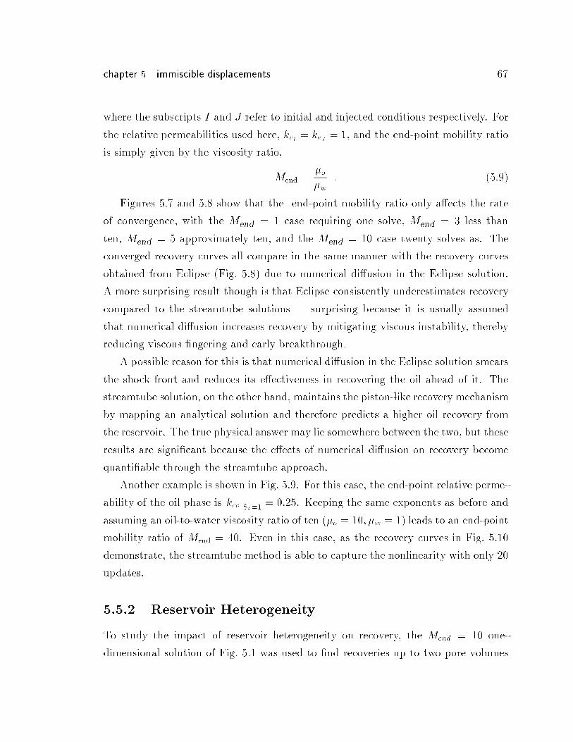
chapter 5 immiscible displacements 67
where the subscripts I and J refer to initial and injected conditions respectively. For
the relative permeabilities used here, krI = krJ = 1, and the end-point mobility ratio
is simply given by the viscosity ratio,
Mend =�o
�w: (5:9)
Figures 5.7 and 5.8 show that the end-point mobility ratio only a�ects the rate
of convergence, with the Mend = 1 case requiring one solve, Mend = 3 less than
ten, Mend = 5 approximately ten, and the Mend = 10 case twenty solves as. The
converged recovery curves all compare in the same manner with the recovery curves
obtained from Eclipse (Fig. 5.8) due to numerical di�usion in the Eclipse solution.
A more surprising result though is that Eclipse consistently underestimates recovery
compared to the streamtube solutions | surprising because it is usually assumed
that numerical di�usion increases recovery by mitigating viscous instability, thereby
reducing viscous �ngering and early breakthrough.
A possible reason for this is that numerical di�usion in the Eclipse solution smears
the shock front and reduces its e�ectiveness in recovering the oil ahead of it. The
streamtube solution, on the other hand, maintains the piston-like recovery mechanism
by mapping an analytical solution and therefore predicts a higher oil recovery from
the reservoir. The true physical answer may lie somewhere between the two, but these
results are signi�cant because the e�ects of numerical di�usion on recovery become
quanti�able through the streamtube approach.
Another example is shown in Fig. 5.9. For this case, the end-point relative perme-
ability of the oil phase is krojSo=1 = 0:25. Keeping the same exponents as before and
assuming an oil-to-water viscosity ratio of ten (�o = 10; �w = 1) leads to an end-point
mobility ratio of Mend = 40. Even in this case, as the recovery curves in Fig. 5.10
demonstrate, the streamtube method is able to capture the nonlinearity with only 20
updates.
5.5.2 Reservoir Heterogeneity
To study the impact of reservoir heterogeneity on recovery, the Mend = 10 one-
dimensional solution of Fig. 5.1 was used to �nd recoveries up to two pore volumes
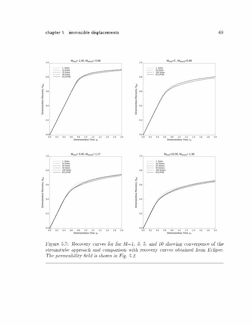
chapter 5 immiscible displacements 68
0.0
0.2
0.4
0.6
0.8
1.0
Dim
ensi
onle
ss R
ecov
ery,
NpD
0.0 0.2 0.4 0.6 0.8 1.0 1.2 1.4 1.6 1.8 2.0Dimensionless Time, tD
Mend= 1.00, Mshock= 0.58
1 Solve10 Solve20 Solve40 SolveECLIPSE
0.0
0.2
0.4
0.6
0.8
1.0
Dim
ensi
onle
ss R
ecov
ery,
NpD
0.0 0.2 0.4 0.6 0.8 1.0 1.2 1.4 1.6 1.8 2.0Dimensionless Time, tD
Mend=3 , Mshock=0.99
1 Solve10 Solve100 SolveECLIPSE
0.0
0.2
0.4
0.6
0.8
1.0
Dim
ensi
onle
ss R
ecov
ery,
NpD
0.0 0.2 0.4 0.6 0.8 1.0 1.2 1.4 1.6 1.8 2.0Dimensionless Time, tD
Mend= 5.00, Mshock= 1.17
1 Solve10 Solve20 Solve40 Solve100 SolveECLIPSE
0.0
0.2
0.4
0.6
0.8
1.0
Dim
ensi
onle
ss R
ecov
ery,
NpD
0.0 0.2 0.4 0.6 0.8 1.0 1.2 1.4 1.6 1.8 2.0Dimensionless Time, tD
Mend=10.00, Mshock= 1.36
1 Solve10 Solves20 Solves40 Solves100 SolvesECLIPSE
Figure 5.7: Recovery curves for for M=1, 3, 5, and 10 showing convergence of thestreamtube approach and comparison with recovery curves obtained from Eclipse.
The permeability �eld is shown in Fig. 5.2.
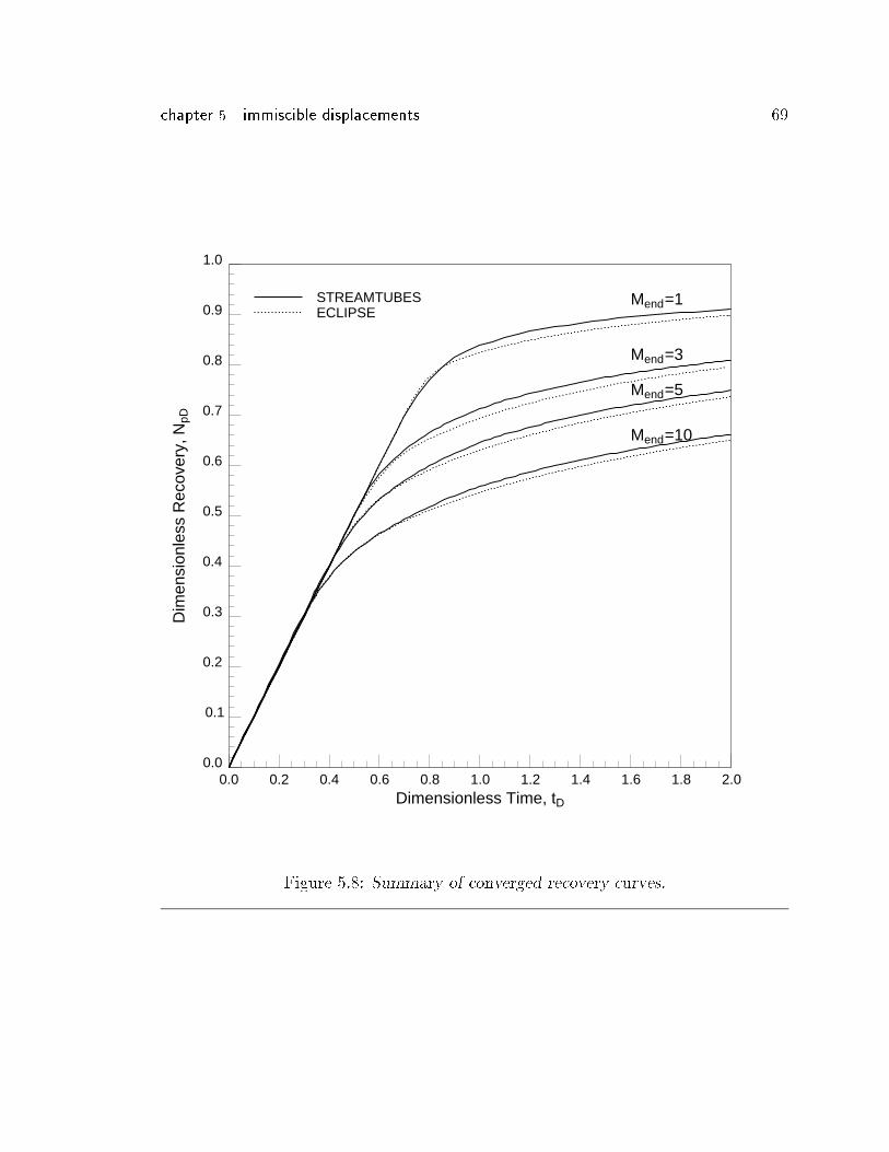
chapter 5 immiscible displacements 69
0.0
0.1
0.2
0.3
0.4
0.5
0.6
0.7
0.8
0.9
1.0
Dim
ensi
onle
ss R
ecov
ery,
NpD
0.0 0.2 0.4 0.6 0.8 1.0 1.2 1.4 1.6 1.8 2.0Dimensionless Time, tD
STREAMTUBESECLIPSE
Mend=1
Mend=3
Mend=5
Mend=10
Figure 5.8: Summary of converged recovery curves.
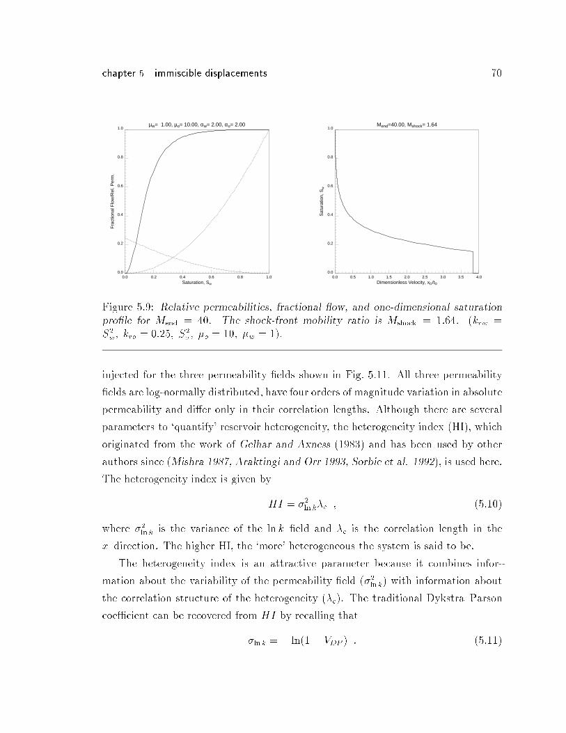
chapter 5 immiscible displacements 70
0.0
0.2
0.4
0.6
0.8
1.0
Sat
urat
ion,
Sw
0.0 0.5 1.0 1.5 2.0 2.5 3.0 3.5 4.0Dimensionless Velocity, xD/tD
Mend=40.00, Mshock= 1.64
0.0
0.2
0.4
0.6
0.8
1.0
Fra
ctio
nal F
low
/Rel
. Per
m.
0.0 0.2 0.4 0.6 0.8 1.0Saturation, Sw
µw= 1.00, µo= 10.00, αw= 2.00, αo= 2.00
Figure 5.9: Relative permeabilities, fractional ow, and one-dimensional saturationpro�le for Mend = 40. The shock-front mobility ratio is Mshock = 1:64. (krw =S2w; kro = 0:25; S2
o; �o = 10; �w = 1).
injected for the three permeability �elds shown in Fig. 5.11. All three permeability
�elds are log-normally distributed, have four orders of magnitude variation in absolute
permeability and di�er only in their correlation lengths. Although there are several
parameters to `quantify' reservoir heterogeneity, the heterogeneity index (HI), which
originated from the work of Gelhar and Axness (1983) and has been used by other
authors since (Mishra 1987, Araktingi and Orr 1993, Sorbie et al. 1992), is used here.
The heterogeneity index is given by
HI = �2ln k�c ; (5:10)
where �2ln k is the variance of the ln k{�eld and �c is the correlation length in the
x{direction. The higher HI, the `more' heterogeneous the system is said to be.
The heterogeneity index is an attractive parameter because it combines infor-
mation about the variability of the permeability �eld (�2ln k) with information about
the correlation structure of the heterogeneity (�c). The traditional Dykstra{Parson
coe�cient can be recovered from HI by recalling that
�ln k = � ln(1� VDP ) : (5:11)
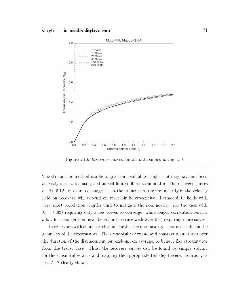
chapter 5 immiscible displacements 71
0.0
0.2
0.4
0.6
0.8
1.0
Dim
ensi
onle
ss R
ecov
ery,
NpD
0.0 0.2 0.4 0.6 0.8 1.0 1.2 1.4 1.6 1.8 2.0Dimensionless Time, tD
Mend=40, Mshock=1.64
1 Solve10 Solve20 Solve40 Solve100 SolveECLIPSE
Figure 5.10: Recovery curves for the data shown in Fig. 5.9.
The streamtube method is able to give some valuable insight that may have not been
as easily observable using a standard �nite di�erence simulator. The recovery curves
of Fig. 5.12, for example, suggest that the in uence of the nonlinearity in the velocity
�eld on recovery will depend on reservoir heterogeneity. Permeability �elds with
very short correlation lengths tend to mitigate the nonlinearity (see the case with
�c = 0:02) requiring only a few solves to converge, while longer correlation lengths
allow for stronger nonlinear behavior (see case with �c = 0:6) requiring more solves.
In reservoirs with short correlation lengths, the nonlinearity is not noticeable in the
geometry of the streamtubes. The streamtubes expand and contract many times over
the duration of the displacement but end{up, on average, to behave like streamtubes
from the tracer case. Thus, the recovery curves can be found by simply solving
for the streamtubes once and mapping the appropriate Buckley-Leverett solution, as
Fig. 5.12 clearly shows.
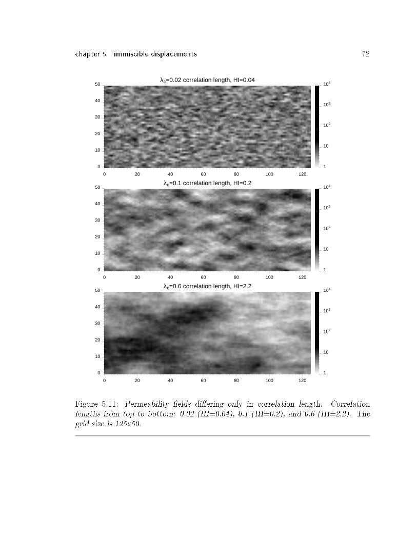
chapter 5 immiscible displacements 72
0
10
20
30
40
50
0 20 40 60 80 100 120
λc=0.02 correlation length, HI=0.04
1
10
102
103
104
0
10
20
30
40
50
0 20 40 60 80 100 120
λc=0.1 correlation length, HI=0.2
1
10
102
103
104
0
10
20
30
40
50
0 20 40 60 80 100 120
λc=0.6 correlation length, HI=2.2
1
10
102
103
104
Figure 5.11: Permeability �elds di�ering only in correlation length. Correlationlengths from top to bottom: 0.02 (HI=0.04), 0.1 (HI=0.2), and 0.6 (HI=2.2). The
grid size is 125x50.
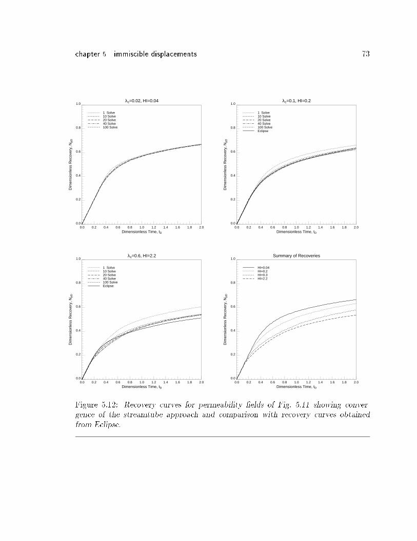
chapter 5 immiscible displacements 73
0.0
0.2
0.4
0.6
0.8
1.0
Dim
ensi
onle
ss R
ecov
ery,
NpD
0.0 0.2 0.4 0.6 0.8 1.0 1.2 1.4 1.6 1.8 2.0Dimensionless Time, tD
λc=0.02, HI=0.04
1 Solve10 Solve20 Solve40 Solve100 Solve
0.0
0.2
0.4
0.6
0.8
1.0
Dim
ensi
onle
ss R
ecov
ery,
NpD
0.0 0.2 0.4 0.6 0.8 1.0 1.2 1.4 1.6 1.8 2.0Dimensionless Time, tD
λc=0.1, HI=0.2
1 Solve10 Solve20 Solve40 Solve100 SolveEclipse
0.0
0.2
0.4
0.6
0.8
1.0
Dim
ensi
onle
ss R
ecov
ery,
NpD
0.0 0.2 0.4 0.6 0.8 1.0 1.2 1.4 1.6 1.8 2.0Dimensionless Time, tD
λc=0.6, HI=2.2
1 Solve10 Solve20 Solve40 Solve100 SolveEclipse
0.0
0.2
0.4
0.6
0.8
1.0
Dim
ensi
onle
ss R
ecov
ery,
NpD
0.0 0.2 0.4 0.6 0.8 1.0 1.2 1.4 1.6 1.8 2.0Dimensionless Time, tD
Summary of Recoveries
HI=0.04HI=0.2HI=0.3HI=2.2
Figure 5.12: Recovery curves for permeability �elds of Fig. 5.11 showing conver-gence of the streamtube approach and comparison with recovery curves obtained
from Eclipse.
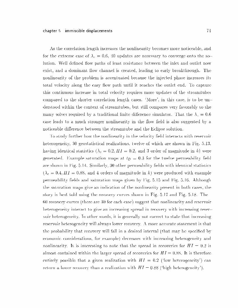
chapter 5 immiscible displacements 74
As the correlation length increases the nonlinearity becomes more noticeable, and
for the extreme case of �c = 0:6, 40 updates are necessary to converge onto the so-
lution. Well de�ned ow paths of least resistance between the inlet and outlet now
exist, and a dominant ow channel is created, leading to early breakthrough. The
nonlinearity of the problem is accentuated because the injected phase increases its
total velocity along the easy ow path until it reaches the outlet end. To capture
this continuous increase in total velocity requires more updates of the streamtubes
compared to the shorter correlation length cases. `More', in this case, is to be un-
derstood within the context of streamtubes, but still compares very favorably to the
many solves required by a traditional �nite di�erence simulator. That the �c = 0:6
case leads to a much stronger nonlinearity in the ow �eld is also suggested by a
noticeable di�erence between the streamtube and the Eclipse solution.
To study further how the nonlinearity in the velocity �eld interacts with reservoir
heterogeneity, 30 geostatistical realizations, twelve of which are shown in Fig. 5.13,
having identical statistics (�c = 0:2;HI = 0:2, and 3 order of magnitude in k) were
generated. Example saturation maps at tD = 0:3 for the twelve permeability �eld
are shown in Fig. 5.14. Similarly, 30 other permeability �elds with identical statistics
(�c = 0:4;HI = 0:88, and 4 orders of magnitude in k) were produced with example
permeability �elds and saturation maps given by Fig. 5.15 and Fig. 5.16. Although
the saturation maps give an indication of the nonlinearity present in both cases, the
story is best told using the recovery curves shown in Fig. 5.17 and Fig. 5.18. The
60 recovery curves (there are 30 for each case) suggest that nonlinearity and reservoir
heterogeneity interact to give an increasing spread in recovery with increasing reser-
voir heterogeneity. In other words, it is generally not correct to state that increasing
reservoir heterogeneity will always lower recovery. A more accurate statement is that
the probability that recovery will fall in a desired interval (that may be speci�ed by
economic considerations, for example) decreases with increasing heterogeneity and
nonlinearity. It is interesting to note that the spread in recoveries for HI = 0:2 is
almost contained within the larger spread of recoveries for HI = 0:88. It is therefore
entirely possible that a given realization with HI = 0:2 (`low heterogeneity') can
return a lower recovery than a realization with HI = 0:88 (`high heterogeneity').
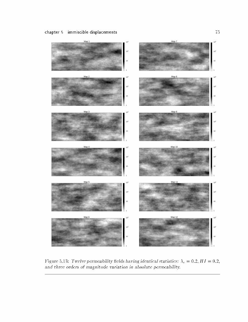
chapter 5 immiscible displacements 75
Map 1
1
10
102
103
Map 2
1
10
102
103
Map 3
1
10
102
103
Map 4
1
10
102
103
Map 5
1
10
102
103
Map 6
1
10
102
103
Map 7
1
10
102
103
Map 8
1
10
102
103
Map 9
1
10
102
103
Map 10
1
10
102
103
Map 11
1
10
102
103
Map 12
1
10
102
103
Figure 5.13: Twelve permeability �elds having identical statistics: �c = 0:2;HI = 0:2,and three orders of magnitude variation in absolute permeability.
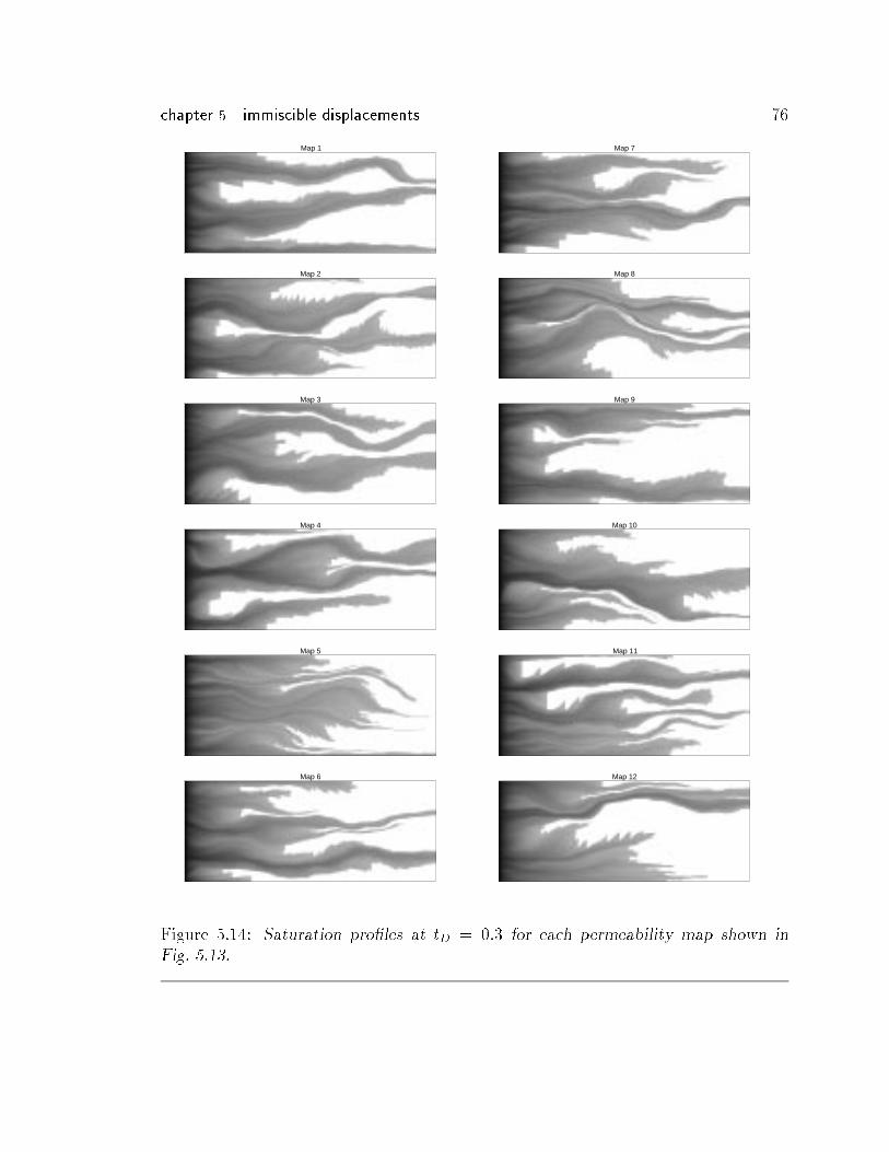
chapter 5 immiscible displacements 76
Map 1
Map 2
Map 3
Map 4
Map 5
Map 6
Map 7
Map 8
Map 9
Map 10
Map 11
Map 12
Figure 5.14: Saturation pro�les at tD = 0:3 for each permeability map shown inFig. 5.13.
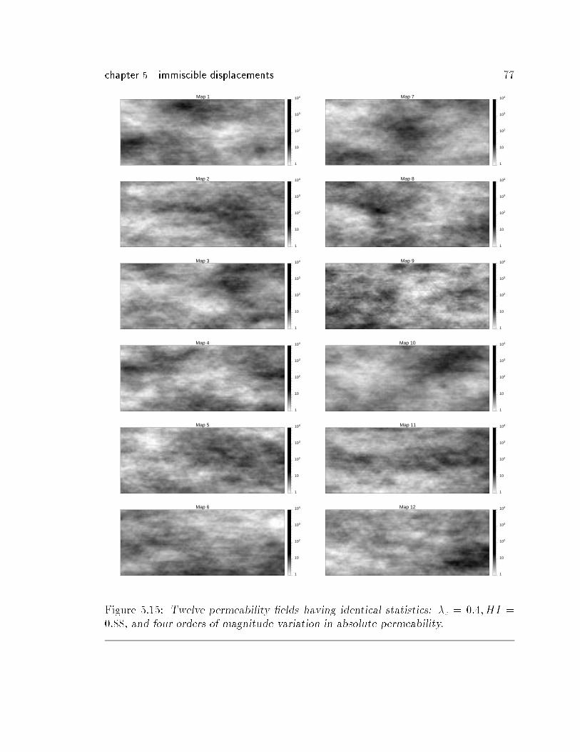
chapter 5 immiscible displacements 77
Map 1
1
10
102
103
104
Map 2
1
10
102
103
104
Map 3
1
10
102
103
104
Map 4
1
10
102
103
104
Map 5
1
10
102
103
104
Map 6
1
10
102
103
104
Map 7
1
10
102
103
104
Map 8
1
10
102
103
104
Map 9
1
10
102
103
104
Map 10
1
10
102
103
104
Map 11
1
10
102
103
104
Map 12
1
10
102
103
104
Figure 5.15: Twelve permeability �elds having identical statistics: �c = 0:4;HI =0:88, and four orders of magnitude variation in absolute permeability.
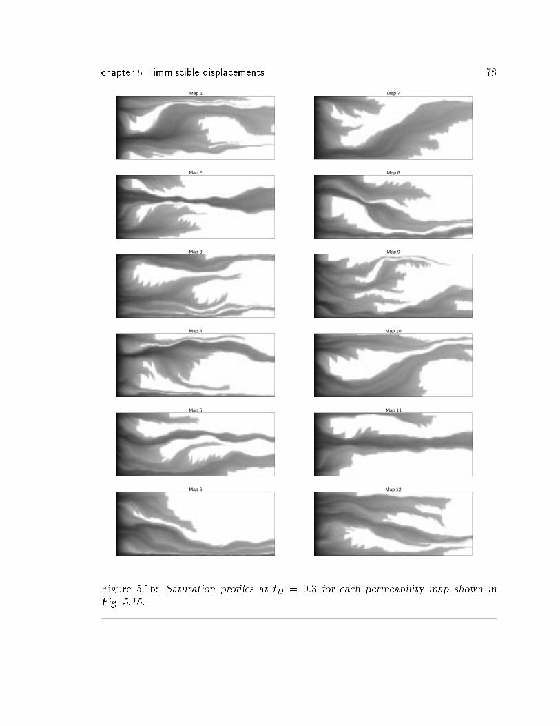
chapter 5 immiscible displacements 78
Map 1
Map 2
Map 3
Map 4
Map 5
Map 6
Map 7
Map 8
Map 9
Map 10
Map 11
Map 12
Figure 5.16: Saturation pro�les at tD = 0:3 for each permeability map shown inFig. 5.15.
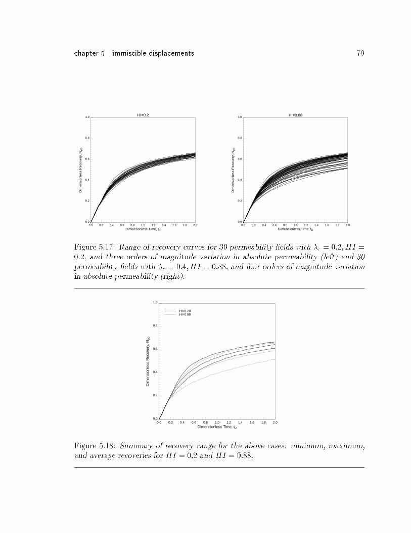
chapter 5 immiscible displacements 79
0.0
0.2
0.4
0.6
0.8
1.0
Dim
ensi
onle
ss R
ecov
ery,
NpD
0.0 0.2 0.4 0.6 0.8 1.0 1.2 1.4 1.6 1.8 2.0Dimensionless Time, tD
HI=0.2
0.0
0.2
0.4
0.6
0.8
1.0
Dim
ensi
onle
ss R
ecov
ery,
NpD
0.0 0.2 0.4 0.6 0.8 1.0 1.2 1.4 1.6 1.8 2.0Dimensionless Time, tD
HI=0.88
Figure 5.17: Range of recovery curves for 30 permeability �elds with �c = 0:2; HI =0:2, and three orders of magnitude variation in absolute permeability (left) and 30permeability �elds with �c = 0:4;HI = 0:88, and four orders of magnitude variationin absolute permeability (right).
0.0
0.2
0.4
0.6
0.8
1.0
Dim
ensi
onle
ss R
ecov
ery,
NpD
0.0 0.2 0.4 0.6 0.8 1.0 1.2 1.4 1.6 1.8 2.0Dimensionless Time, tD
HI=0.20HI=0.88
Figure 5.18: Summary of recovery range for the above cases: minimum, maximum,
and average recoveries for HI = 0:2 and HI = 0:88.
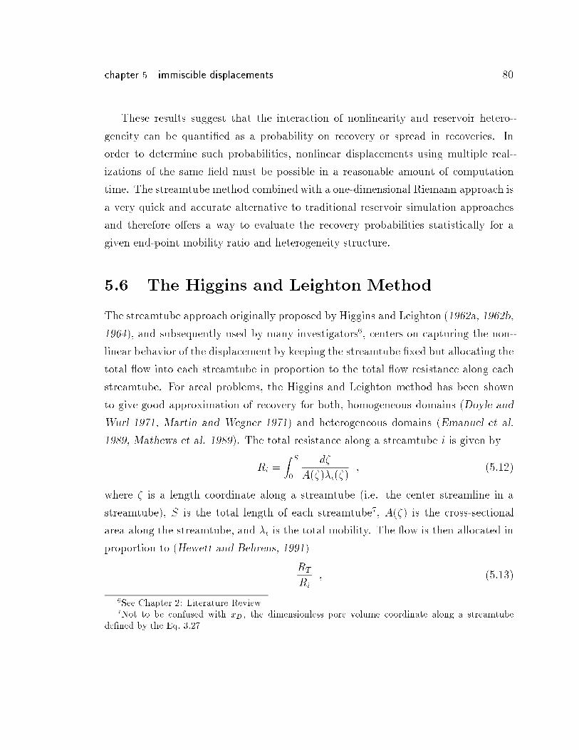
chapter 5 immiscible displacements 80
These results suggest that the interaction of nonlinearity and reservoir hetero-
geneity can be quanti�ed as a probability on recovery or spread in recoveries. In
order to determine such probabilities, nonlinear displacements using multiple real-
izations of the same �eld must be possible in a reasonable amount of computation
time. The streamtube method combined with a one-dimensional Riemann approach is
a very quick and accurate alternative to traditional reservoir simulation approaches
and therefore o�ers a way to evaluate the recovery probabilities statistically for a
given end-point mobility ratio and heterogeneity structure.
5.6 The Higgins and Leighton Method
The streamtube approach originally proposed by Higgins and Leighton (1962a, 1962b,
1964), and subsequently used by many investigators6, centers on capturing the non-
linear behavior of the displacement by keeping the streamtube �xed but allocating the
total ow into each streamtube in proportion to the total ow resistance along each
streamtube. For areal problems, the Higgins and Leighton method has been shown
to give good approximation of recovery for both, homogeneous domains (Doyle and
Wurl 1971, Martin and Wegner 1971) and heterogeneous domains (Emanuel et al.
1989, Mathews et al. 1989). The total resistance along a streamtube i is given by
Ri =Z
S
0
d�
A(�)�t(�); (5:12)
where � is a length coordinate along a streamtube (i.e. the center streamline in a
streamtube), S is the total length of each streamtube7, A(�) is the cross-sectional
area along the streamtube, and �t is the total mobility. The ow is then allocated in
proportion to (Hewett and Behrens, 1991)
RT
Ri
; (5:13)
6See Chapter 2: Literature Review7Not to be confused with xD, the dimensionless pore volume coordinate along a streamtube
de�ned by the Eq. 3.27
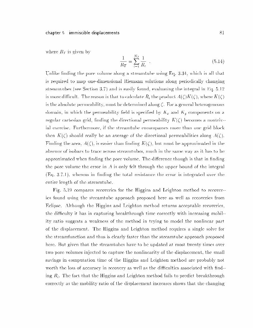
chapter 5 immiscible displacements 81
where RT is given by
1
RT
=NSXi=1
1
Ri
: (5:14)
Unlike �nding the pore volume along a streamtube using Eq. 3.34, which is all that
is required to map one-dimensional Riemann solutions along periodically changing
streamtubes (see Section 3.7) and is easily found, evaluating the integral in Eq. 5.12
is more di�cult. The reason is that to calculate Ri the product A(�)K(�), whereK(�)
is the absolute permeability, must be determined along �. For a general heterogeneous
domain, in which the permeability �eld is speci�ed by Kx and Ky components on a
regular cartesian grid, �nding the directional permeability K(�) becomes a nontriv-
ial exercise. Furthermore, if the streamtube encompasses more than one grid block
then K(�) should really be an average of the directional permeabilities along A(�).
Finding the area, A(�), is easier than �nding K(�), but must be approximated in the
absence of isobars to trace across streamtubes, much in the same way as it has to be
approximated when �nding the pore volume. The di�erence though is that in �nding
the pore volume the error in A is only felt through the upper bound of the integral
(Eq. 3.7.1), whereas in �nding the total resistance the error is integrated over the
entire length of the streamtube.
Fig. 5.19 compares recoveries for the Higgins and Leighton method to recover-
ies found using the streamtube approach proposed here as well as recoveries from
Eclipse. Although the Higgins and Leighton method returns acceptable recoveries,
the di�culty it has in capturing breakthrough time correctly with increasing mobil-
ity ratio suggests a weakness of the method in trying to model the nonlinear part
of the displacement. The Higgins and Leighton method requires a single solve for
the streamfunction and thus is clearly faster than the streamtube approach proposed
here. But given that the streamtubes have to be updated at most twenty times over
two pore volumes injected to capture the nonlinearity of the displacement, the small
savings in computation time of the Higgins and Leighton method are probably not
worth the loss of accuracy in recovery as well as the di�culties associated with �nd-
ing Ri. The fact that the Higgins and Leighton method fails to predict breakthrough
correctly as the mobility ratio of the displacement increases shows that the changing
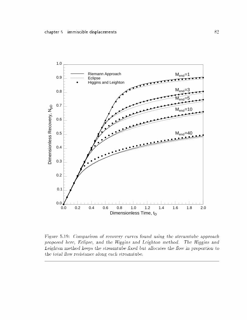
chapter 5 immiscible displacements 82
0.0
0.1
0.2
0.3
0.4
0.5
0.6
0.7
0.8
0.9
1.0
Dim
ensi
onle
ss R
ecov
ery,
NpD
0.0 0.2 0.4 0.6 0.8 1.0 1.2 1.4 1.6 1.8 2.0Dimensionless Time, tD
a
a
a
a
a
a
a
a
a
a
a
a
a
a
a
a
a
aaaa a a a a a a a a a a a a a a a a a a a a
a
a
a
a
a
a
a
a
a
a
a
a
a
a
aaaaaaaa a a a a a a a a a a a a a a a a a a a
a
a
a
a
a
a
a
a
a
a
a
a
aaaaaaaaa a a a a a a a a a a a a a a a a a a a a
a
a
a
a
a
a
a
a
a
a
aaaaaaaaa a a a a a a a a a a a a a a a a a a a a a a
a
a
a
a
a
a
aaaaaaaa a a a a a a a a a a a a a a a a a a a a a a a a a a a
a
Riemann ApproachEclipseHiggins and Leighton
Mend=1
Mend=3
Mend=5
Mend=10
Mend=40
Figure 5.19: Comparison of recovery curves found using the streamtube approachproposed here, Eclipse, and the Higgins and Leighton method. The Higgins and
Leighton method keeps the streamtube �xed but allocates the ow in proportion to
the total ow resistance along each streamtube.
chapter 5 immiscible displacements 83
velocity can only roughly be approximated using a �xed streamtube/total resistance
approach.
5.7 Concluding Remarks
In this chapter, the streamtube approach was extended to model two{phase, immis-
cible displacements. To account for the changing total velocity �eld, the streamtubes
were updated periodically. The one{dimensional Buckley{Leverett solution was then
mapped along the new streamtubes as a true Riemann solution. The key result of this
chapter is to demonstrate that the error caused by the Riemann approach used for
mapping a one{dimensional solution along periodically updated streamtubes is small
and, in fact, is less signi�cant than the error introduced by numerical di�usion in �-
nite di�erence solutions. Another key result is that the weak nonlinearity of the total
velocity �eld allows for converged solutions using at most 20 streamtube updates over
two pore volumes. As a result, speed{ups by two orders of magnitude with respect
to traditional �nite di�erence solutions are achieved. The speed of the streamtube
method is put to use in a statistical approach to reservoir forecasting, demonstrating
that the spread in recovery due to equiprobable permeability �elds can be substantial.
The spread in recovery is particularly important, because it suggests that the error
caused by the numerical scheme itself may be small compared to the uncertainty intro-
duced by the statistics of the reservoir description. Finally, the streamtube approach
proposed here was also compared to the Higgins and Leighton method, demonstrating
that the nonlinear part of the ow problem cannot be accounted for by using a �xed
streamtube/total resistance approach. In the next chapter, the streamtube approach
is extended to ideal miscible displacements.
Chapter 6
First-Contact Miscible
Displacements
This chapter applies the streamtube approach to modeling �rst contact miscible
(FCM) displacements through heterogeneous reservoirs. Three one-dimensional so-
lutions are presented that may be combined with streamtubes to construct two-
dimensional solutions for heterogeneous systems: (1) a piston-like, unit wave velocity
solution, (2) a convection-di�usion solution, and (3) a viscous �ngering solution. The
displacement scale implied by each of these three one-dimensional solutions is dis-
cussed. The resulting two-dimensional streamtube solutions are shown to capture
overall recovery and �rst-order displacement features seen in traditional �nite dif-
ference solutions. The superior speed of the streamtube solution is put to use in
a statistical approach to reservoir forecasting: recovery curves for 180 permeability
�elds are used to demonstrate how nonlinearity in the total velocity �eld and hetero-
geneity interact to determine overall recovery.
6.1 Introduction
First-contact miscible (FCM) displacements1 in heterogeneous systems have been
studied by several authors (Araktingi and Orr, 1993, Gorell 1992, Sorbie et al. 1992,
1Sometimes also referred to as ideal miscible displacements.
84
chapter 6 �rst-contact miscible displacements 85
Waggoner et al. 1992, Christie 1989). An extensive treatment of the subject was
recently given by Tchelepi (1994). The strong interest in �rst-contact miscible dis-
placements is motivated principally by the possibility of learning more about dis-
placements which are near-miscible, such as gas and carbon-dioxide ooding. The
assumptions used in �rst-contact miscible ow isolate the convective part of the dis-
placement problem from any phase behavior considerations and allow a study of the
interaction of reservoir heterogeneity and the nonlinearity of the total velocity �eld in
determining sweep e�ciency. But the absence of any phase behavior and multiphase
ow aspects enhances the nonlinearity of the problem. Di�usive mechanisms, such as
molecular di�usion and pore scale mixing, are the only physical mechanisms available
to mitigate the original mobility contrast. As a result, �rst-contact miscible displace-
ments are very challenging to simulate numerically and are far more di�cult than the
two-phase immiscible problem discussed in Chapter 5. High mobility contrasts lead
to extreme velocity variations and su�cient grid blocks must be used to ensure that
numerical di�usion is as close as possible to representing true physical di�usion at the
grid block scale. To �nd physically meaningful simulations of �rst-contact miscible
displacements require substantial computer resources (Tchelepi 1994, Christie and
Bond 1987).
6.2 The Assumptions in FCM Flow
The assumptions for �rst-contact miscible ow are analogous to the assumptions used
to derive the tracer solution presented in Chapter 4. The general material balance
formulation for a component i with no chemical reactions and adsorption/desorption
given by (Lake 1989, p. 29) is
@
@t
0@� NPX
j=1
�jSj!ij
1A +r �
0@NPXj=1
�j!ij~uj � �Sj�j~~Kij � r!ij
1A = 0; (6:1)
and assuming (a) single-phase ow, (b) incompressible uid and rock properties, (c)
constant phase density, and (d) ideal mixing gives
�@Ci
@t+r �
�Ci~u� �
~~Ki � rCi
�= 0 : (6:2)
chapter 6 �rst-contact miscible displacements 86
Expanding the divergence term in Eq. 6.2 and applying continuity (r � ~u = 0) gives
the governing equation for miscible displacements as
�@Ci
@t+ ~u � rCi � �r �
�~~Ki � rCi
�= 0 : (6:3)
Eq. 6.3 is identical to the tracer formulation. The di�erence is hidden in the Darcy
velocity ~u which is now given by
~u =~~k
�(C)� rP ; (6:4)
where the viscosity � is assumed a function of concentration C. A quarter power
mixing rule, given by
�(C) =
C
�1=4s
+1� C
�1=4o
!�4
; (6:5)
is usually used as a functional relationship between � and C. �s is the `solvent'
viscosity and �o is the `oil' viscosity, which are simply the viscosities at C = 1 and
C = 0 respectively, and also de�ne the end-point mobility ratio as
M =�o
�s: (6:6)
Eq. 6.3 is the starting PDE for all �rst-contact miscible unstable displacements. The
`strength' of the nonlinearity in the ow �eld will depend on the coupling between
Eq. 6.3 and Eq. 6.4 through the mixture viscosity, �(C), and the relative magnitude
of the convective term (~u � rCi) to the di�usive term (r � ~~Ki � rCi). If the di�usive
term is large compared the convective term (small Peclet numbers), then instabilities
will tend to be mitigated. Conversely, if the convective term dominates, then the
displacement will see the growth of viscous �ngers and/or strong channeling. It is
therefore important to use a numerical scheme that will ensure a numerical di�usion
term (which behaves much in the same way as physical di�usion) that is small |
preferably on the order of the physical di�usion that is expected at the local grid
block level| so as not to mask the true physics of the displacement.
chapter 6 �rst-contact miscible displacements 87
6.3 The One-Dimensional Solution(s)
The use of streamtubes to model �rst-contact miscible displacements in heteroge-
neous systems requires a one-dimensional solution. For �rst-contact miscible ow,
the governing one-dimensional PDE is easily derived from Eq. 6.3 as
�@Ci
@t+ u
@Ci
@x� �
@
@xKi
@Ci
@x= 0 : (6:7)
Using the usual de�nitions of dimensionless time, distance, and concentration assum-
ing two components only, and a spatially constant Ki gives the familiar convection-
di�usion equation@CD
@tD+@CD
@xD=
1
NPe
@2CD
@x2D
: (6:8)
Eq. 6.8 is linear. The nonlinearity of the problem is accounted for by the coe�cients in
the governing PDE for the streamfunction that include the concentration-dependent
viscosity@
@x
�(CD)
ky
@
@x
!+
@
@y
�(CD)
kx
@
@y
!= 0 : (6:9)
Thus, as the spatial concentration distribution changes, the coe�cients of Eq. 6.9
change resulting in new streamtubes.
Unlike the two-phase immiscible problem, the �rst-contact miscible case has a
subtle one-dimensional solution. For example, the no-di�usion form of Eq. 6.8 is
given by@CD
@tD+@CD
@xD= 0 : (6:10)
Eq. 6.10 is of hyperbolic type (Zauderer 1989) and can be solved using initial data of
the type (Riemann conditions)
CD(xD; 0)
8<: CDl for xD � 0
CDr for xD � 0; (6:11)
giving the well-known indi�erent wave solution traveling at unit velocity (see Fig. 4.3).
For favorable mobility ratios, the `physical' solution is indeed a wave traveling at
unit velocity, although the wave is no longer indi�erent but self-sharpening. For
unfavorable mobility ratios, on the other hand, the solution to Eq. 6.10 is misleading
chapter 6 �rst-contact miscible displacements 88
because it still gives a piston-like displacement, when the system is in fact unstable.
The problem, of course, is that the displacement model given by Eq. 6.10 is unable to
distinguish between stable and unstable displacements since it is linear; by not having
concentration dependent coe�cients, the solution cannot account for any viscosity
induced mobility contrast as a function of xD and tD. Furthermore, Eq. 6.10 has no
characteristic length scale, resulting in a sharp, but unstable front at all length scales
and for all times. A physically meaningful solution, on the other hand, would require
some cut-o� length scale across which the frontal instability is mitigated.
Adding a cut-o� length scale can be done mathematically by retaining the second
order di�usion term in Eq. 6.8. That implies that the cut-o� length scale is now
given by the di�usive length scale associated with NPe. It is important to note
that Eq. 6.7, by its very derivation, has no way of modeling any other instability
mitigation phenomena. In particular, there is no convective induced mixing beyond
the pore scale that can be accounted for.
It is unlikely that at the �eld scale molecular di�usion and pore level mixing are
�rst-order type physical processes that a�ect recovery. Convective mixing at the
macroscale, such as viscous �ngering and channeling are probably more important.
To account for such phenomena in an averaged, one-dimensional sense, an analogy to
two-phase ow was �rst proposed by Koval (1963). In the Koval model, straight line
relative permeabilities and a quarter-power mixing rule are combined to de�ne a ux
function f(CD) that models convective mixing of the uids. The governing PDE for
Koval's model is2
@CD
@tD+@f (CD)
@xD= 0 ; (6:12)
where f (CD) is given by
f (CD) =1
1 + 1�CDCD
1
Me�
: (6:13)
Me� is the e�ective mobility ratio de�ned as
Me� =�0:78 + 0:22M 1=4
�4; (6:14)
2Koval's original model also includes a heterogeneity factor H. This factor is set to H = 1(homogeneous) for all Koval solutions presented in this dissertation, since the model is used only tocapture viscous �ngering in an averaged one-dimensional sense along streamtubes.
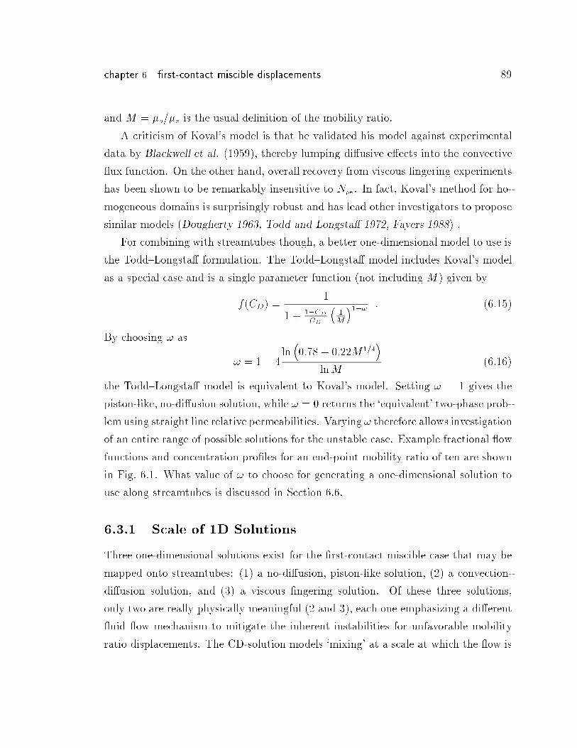
chapter 6 �rst-contact miscible displacements 89
and M = �o=�s is the usual de�nition of the mobility ratio.
A criticism of Koval's model is that he validated his model against experimental
data by Blackwell et al. (1959), thereby lumping di�usive e�ects into the convective
ux function. On the other hand, overall recovery from viscous �ngering experiments
has been shown to be remarkably insensitive to Npe. In fact, Koval's method for ho-
mogeneous domains is surprisingly robust and has lead other investigators to propose
similar models (Dougherty 1963, Todd and Longsta� 1972, Fayers 1988) .
For combining with streamtubes though, a better one-dimensional model to use is
the Todd{Longsta� formulation. The Todd{Longsta� model includes Koval's model
as a special case and is a single parameter function (not including M ) given by
f(CD) =1
1 + 1�CDCD
�1
M
�1�! : (6:15)
By choosing ! as
! = 1� 4ln�0:78 + 0:22M 1=4
�lnM
(6:16)
the Todd{Longsta� model is equivalent to Koval's model. Setting ! = 1 gives the
piston-like, no-di�usion solution, while ! = 0 returns the `equivalent' two-phase prob-
lem using straight line relative permeabilities. Varying ! therefore allows investigation
of an entire range of possible solutions for the unstable case. Example fractional ow
functions and concentration pro�les for an end-point mobility ratio of ten are shown
in Fig. 6.1. What value of ! to choose for generating a one-dimensional solution to
use along streamtubes is discussed in Section 6.6.
6.3.1 Scale of 1D Solutions
Three one-dimensional solutions exist for the �rst-contact miscible case that may be
mapped onto streamtubes: (1) a no-di�usion, piston-like solution, (2) a convection-
di�usion solution, and (3) a viscous �ngering solution. Of these three solutions,
only two are really physically meaningful (2 and 3), each one emphasizing a di�erent
uid ow mechanism to mitigate the inherent instabilities for unfavorable mobility
ratio displacements. The CD-solution models `mixing' at a scale at which the ow is
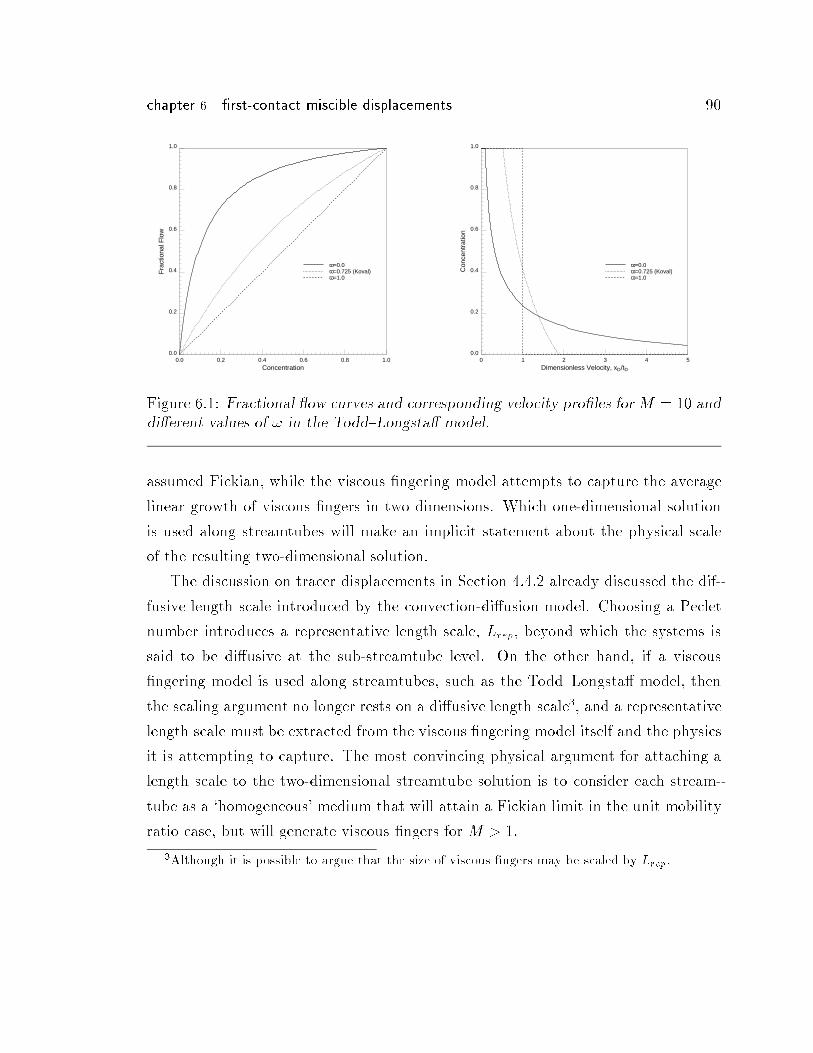
chapter 6 �rst-contact miscible displacements 90
0.0
0.2
0.4
0.6
0.8
1.0
Con
cent
ratio
n
0 1 2 3 4 5Dimensionless Velocity, xD/tD
ω=0.0ω=0.725 (Koval)ω=1.0
0.0
0.2
0.4
0.6
0.8
1.0
Fra
ctio
nal F
low
0.0 0.2 0.4 0.6 0.8 1.0Concentration
ω=0.0ω=0.725 (Koval)ω=1.0
Figure 6.1: Fractional ow curves and corresponding velocity pro�les forM = 10 anddi�erent values of ! in the Todd{Longsta� model.
assumed Fickian, while the viscous �ngering model attempts to capture the average
linear growth of viscous �ngers in two dimensions. Which one-dimensional solution
is used along streamtubes will make an implicit statement about the physical scale
of the resulting two-dimensional solution.
The discussion on tracer displacements in Section 4.4.2 already discussed the dif-
fusive length scale introduced by the convection-di�usion model. Choosing a Peclet
number introduces a representative length scale, Lrep, beyond which the systems is
said to be di�usive at the sub-streamtube level. On the other hand, if a viscous
�ngering model is used along streamtubes, such as the Todd{Longsta� model, then
the scaling argument no longer rests on a di�usive length scale3, and a representative
length scale must be extracted from the viscous �ngering model itself and the physics
it is attempting to capture. The most convincing physical argument for attaching a
length scale to the two-dimensional streamtube solution is to consider each stream-
tube as a `homogeneous' medium that will attain a Fickian limit in the unit mobility
ratio case, but will generate viscous �ngers for M > 1.
3Although it is possible to argue that the size of viscous �ngers may be scaled by Lrep.
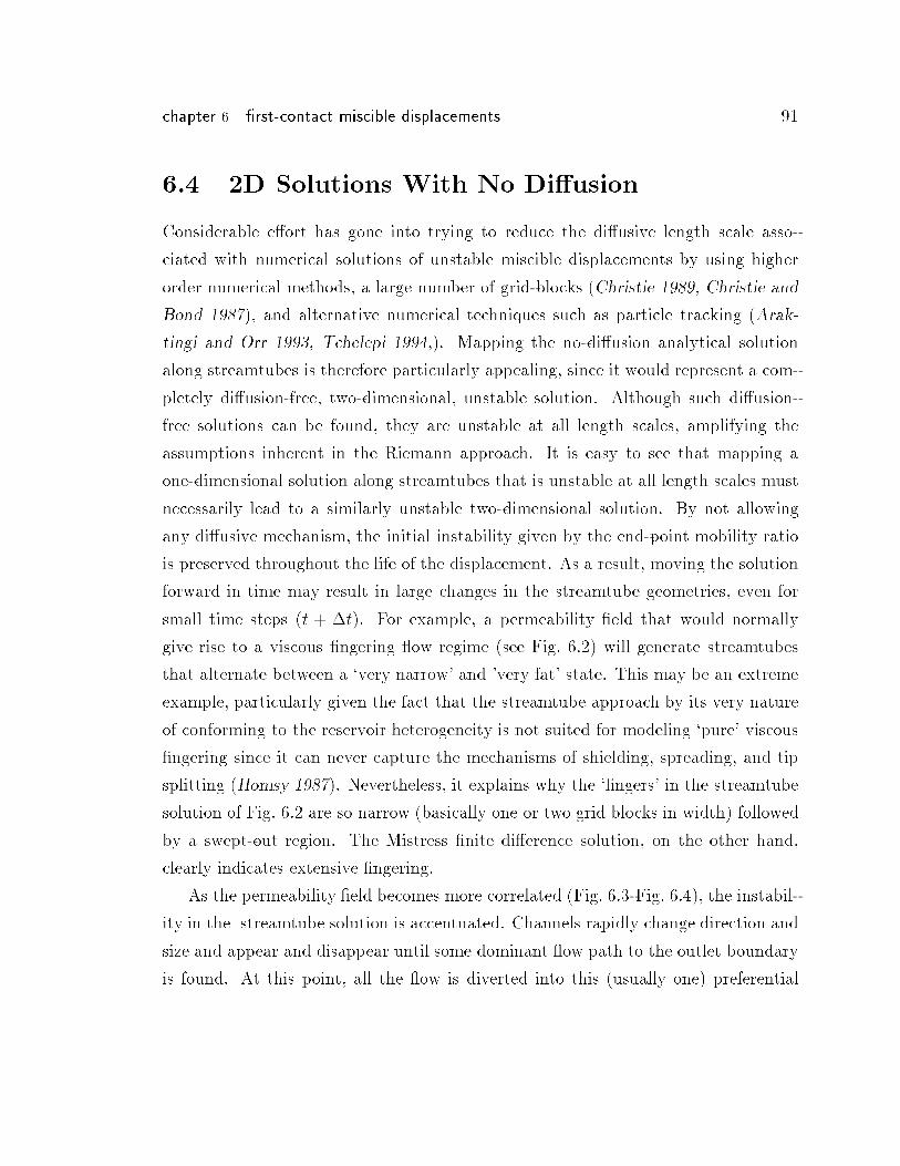
chapter 6 �rst-contact miscible displacements 91
6.4 2D Solutions With No Di�usion
Considerable e�ort has gone into trying to reduce the di�usive length scale asso-
ciated with numerical solutions of unstable miscible displacements by using higher
order numerical methods, a large number of grid-blocks (Christie 1989, Christie and
Bond 1987), and alternative numerical techniques such as particle tracking (Arak-
tingi and Orr 1993, Tchelepi 1994,). Mapping the no-di�usion analytical solution
along streamtubes is therefore particularly appealing, since it would represent a com-
pletely di�usion-free, two-dimensional, unstable solution. Although such di�usion-
free solutions can be found, they are unstable at all length scales, amplifying the
assumptions inherent in the Riemann approach. It is easy to see that mapping a
one-dimensional solution along streamtubes that is unstable at all length scales must
necessarily lead to a similarly unstable two-dimensional solution. By not allowing
any di�usive mechanism, the initial instability given by the end-point mobility ratio
is preserved throughout the life of the displacement. As a result, moving the solution
forward in time may result in large changes in the streamtube geometries, even for
small time steps (t + �t). For example, a permeability �eld that would normally
give rise to a viscous �ngering ow regime (see Fig. 6.2) will generate streamtubes
that alternate between a `very narrow' and 'very fat' state. This may be an extreme
example, particularly given the fact that the streamtube approach by its very nature
of conforming to the reservoir heterogeneity is not suited for modeling `pure' viscous
�ngering since it can never capture the mechanisms of shielding, spreading, and tip
splitting (Homsy 1987). Nevertheless, it explains why the `�ngers' in the streamtube
solution of Fig. 6.2 are so narrow (basically one or two grid blocks in width) followed
by a swept-out region. The Mistress �nite di�erence solution, on the other hand,
clearly indicates extensive �ngering.
As the permeability �eld becomes more correlated (Fig. 6.3-Fig. 6.4), the instabil-
ity in the streamtube solution is accentuated. Channels rapidly change direction and
size and appear and disappear until some dominant ow path to the outlet boundary
is found. At this point, all the ow is diverted into this (usually one) preferential
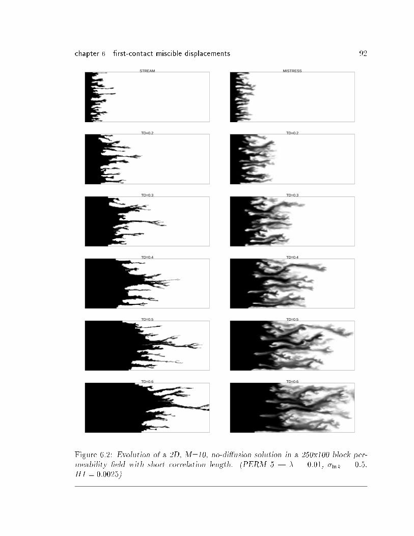
chapter 6 �rst-contact miscible displacements 92
STREAM
TD=0.2
TD=0.3
TD=0.4
TD=0.5
TD=0.6
MISTRESS
TD=0.2
TD=0.3
TD=0.4
TD=0.5
TD=0.6
Figure 6.2: Evolution of a 2D, M=10, no-di�usion solution in a 250x100 block per-
meability �eld with short correlation length. (PERM 5 | � = 0:01, �lnk = 0:5,HI = 0:0025)
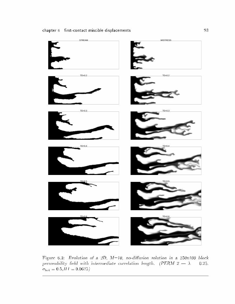
chapter 6 �rst-contact miscible displacements 93
STREAM
TD=0.2
TD=0.3
TD=0.4
TD=0.5
TD=0.6
MISTRESS
TD=0.2
TD=0.3
TD=0.4
TD=0.5
TD=0.6
Figure 6.3: Evolution of a 2D, M=10, no-di�usion solution in a 250x100 block
permeability �eld with intermediate correlation length. (PERM 2 | � = 0:25,�ln k = 0:5,HI = 0:0625)
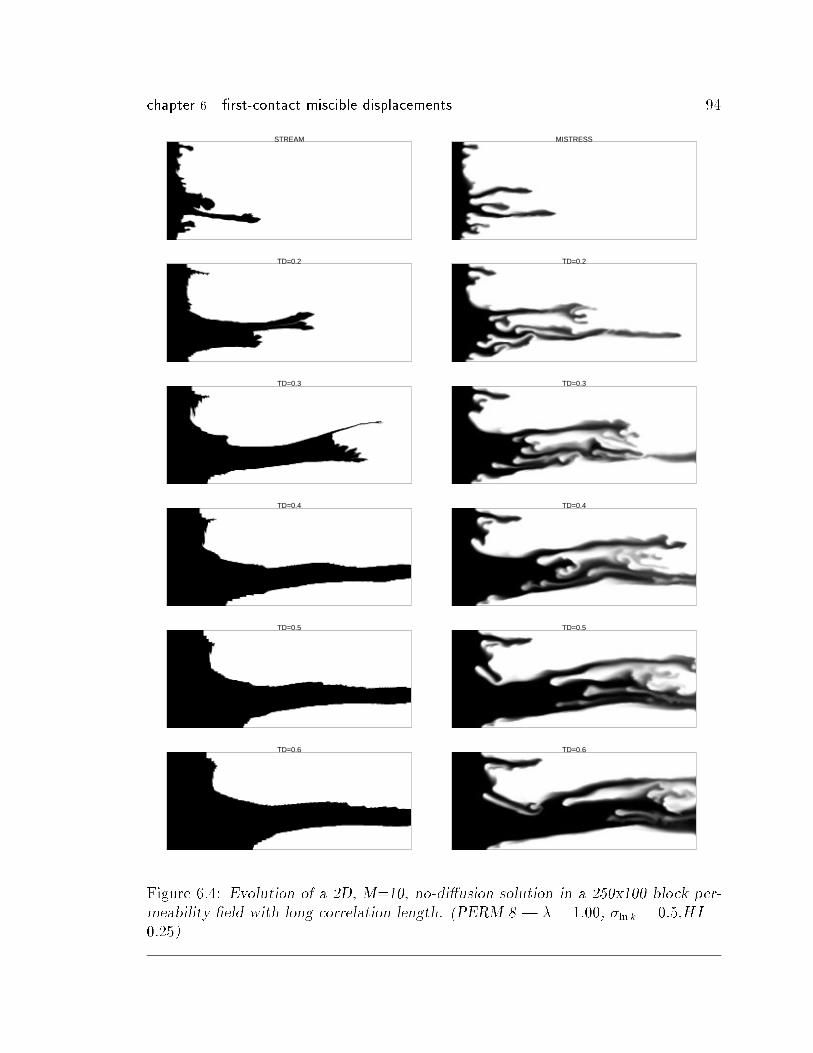
chapter 6 �rst-contact miscible displacements 94
STREAM
TD=0.2
TD=0.3
TD=0.4
TD=0.5
TD=0.6
MISTRESS
TD=0.2
TD=0.3
TD=0.4
TD=0.5
TD=0.6
Figure 6.4: Evolution of a 2D, M=10, no-di�usion solution in a 250x100 block per-
meability �eld with long correlation length. (PERM 8 | � = 1:00, �ln k = 0:5,HI =0:25)
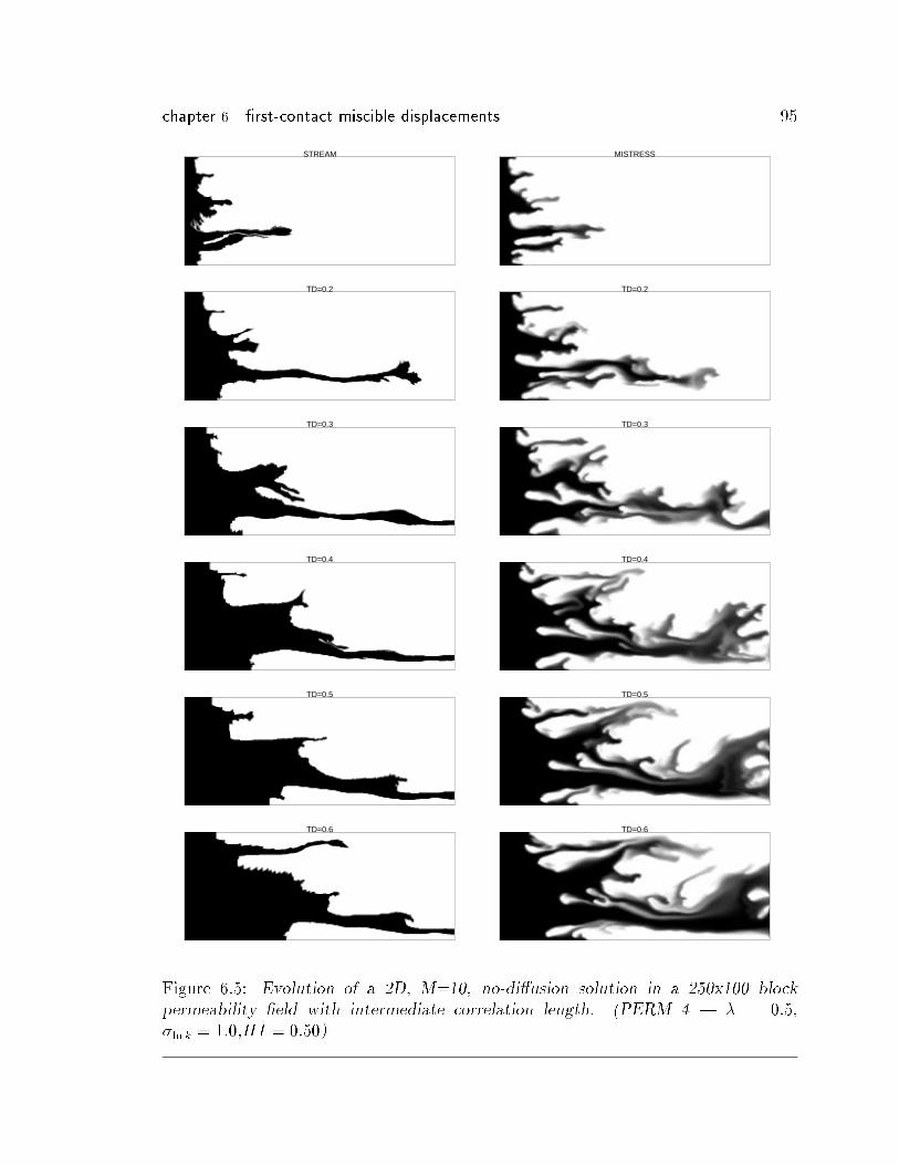
chapter 6 �rst-contact miscible displacements 95
STREAM
TD=0.2
TD=0.3
TD=0.4
TD=0.5
TD=0.6
MISTRESS
TD=0.2
TD=0.3
TD=0.4
TD=0.5
TD=0.6
Figure 6.5: Evolution of a 2D, M=10, no-di�usion solution in a 250x100 block
permeability �eld with intermediate correlation length. (PERM 4 | � = 0:5,�ln k = 1:0,HI = 0:50)
chapter 6 �rst-contact miscible displacements 96
ow path, causing the fronts to retract in many of the other channels, giving the im-
pression of `backwards' ow. Although visible to a certain extent in Fig. 6.2-Fig. 6.4,
the instability of the solution is best demonstrated in an animated version of the dis-
placement. The recovery curves for the di�erent displacements, shown in Fig. 6.6, are
particularly interesting. Given the completely unstable nature of the displacements,
overall recoveries are remarkably good and breakthrough is predicted correctly in all
cases. The reason for this must be that the �rst-order e�ect due to the underlying
heterogeneity structure is still captured by the streamtubes.
Possibly the `best' solution in the no-di�usion case can be obtained for systems
in which the correlation length is on the same order, or greater, of the system length
(�c > L); the least resistant ow path is found immediately and the competition
between several streamtubes never materializes. The problem with systems of this
type is that the large channel(s) could now be considered homogeneous systems in
their own right, giving rise to a viscous �ngering dominated ow regime within them.
Fig. 6.4 shows just that. The streamtube solution correctly identi�es the preferential
ow path, but the �nite di�erence solution does display viscous �ngering within the
channel.
The examples in this section demonstrate that mapping a piston-like, M > 1
solution along the streamtubes results in unstable two-dimensional solutions. All the
solutions were for an end-point mobility ratio of ten (M = 10). Choosing M < 10
would certainly give better behaved solution (in the limit of M = 1 the no-di�usion
tracer solution is obtained), whereas choosing M > 10 would make things worse. As
with the one-dimensional solution, the problem is that there is no characteristic length
scale on which to mitigate the instability, causing streamtubes to abruptly change in
size and direction. Streamtubes are able to �nd dominant ow channels, if they exist,
and are even able to return a particularly good match of breakthrough. Nevertheless,
it is evident that, in general, the solutions will be unstable and nonphysical.
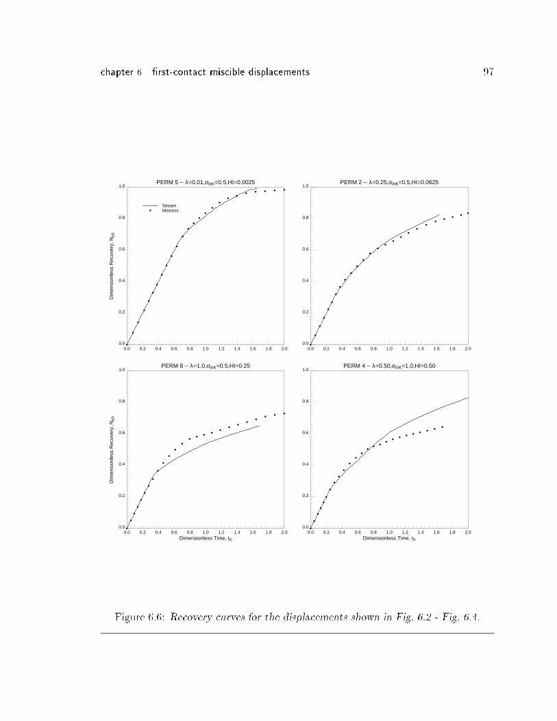
chapter 6 �rst-contact miscible displacements 97
0.0
0.2
0.4
0.6
0.8
1.0
Dim
ensi
onle
ss R
ecov
ery,
NpD
0.0 0.2 0.4 0.6 0.8 1.0 1.2 1.4 1.6 1.8 2.0
PERM 5 -- λ=0.01,σlnK=0.5,HI=0.0025
a
a
a
a
a
a
a
a
a
a
a
a
a
a
a
a
a
a
aa
aa a a a
aStreamMistress
0.0
0.2
0.4
0.6
0.8
1.0
0.0 0.2 0.4 0.6 0.8 1.0 1.2 1.4 1.6 1.8 2.0
PERM 2 -- λ=0.25,σlnK=0.5,HI=0.0625
a
a
a
a
a
a
a
a
a
a
a
a
a
a
a
a
a
a
a
aa
aa
aa
0.0
0.2
0.4
0.6
0.8
1.0
Dim
ensi
onle
ss R
ecov
ery,
NpD
0.0 0.2 0.4 0.6 0.8 1.0 1.2 1.4 1.6 1.8 2.0Dimensionless Time, tD
PERM 8 -- λ=1.0,σlnK=0.5,HI=0.25
a
a
a
a
a
a
a
a
a
a
a
a
a
aa
aa
aa
aa
aa
a a
0.0
0.2
0.4
0.6
0.8
1.0
0.0 0.2 0.4 0.6 0.8 1.0 1.2 1.4 1.6 1.8 2.0Dimensionless Time, tD
PERM 4 -- λ=0.50,σlnK=1.0,HI=0.50
a
a
a
a
a
a
a
a
a
a
a
a
a
aa
aa
aa
aa
aa
aa
Figure 6.6: Recovery curves for the displacements shown in Fig. 6.2 - Fig. 6.4.
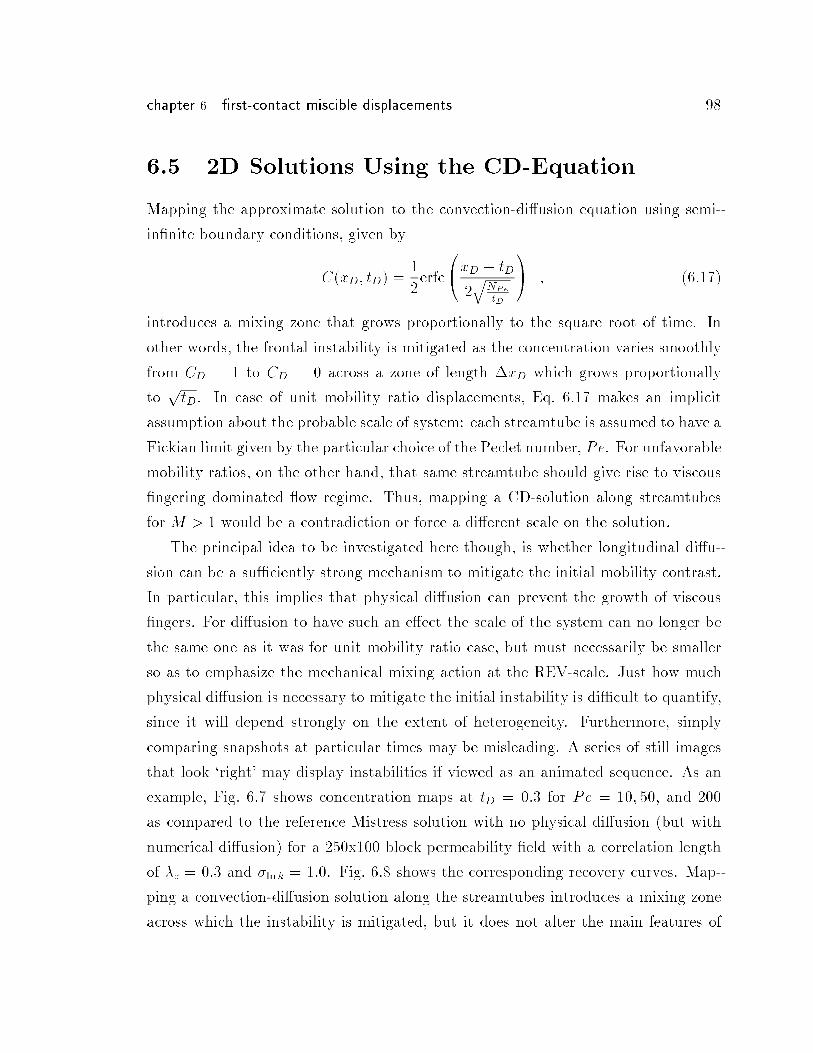
chapter 6 �rst-contact miscible displacements 98
6.5 2D Solutions Using the CD-Equation
Mapping the approximate solution to the convection-di�usion equation using semi-
in�nite boundary conditions, given by
C(xD; tD) =1
2erfc
0@xD � tD
2q
NPe
tD
1A ; (6:17)
introduces a mixing zone that grows proportionally to the square root of time. In
other words, the frontal instability is mitigated as the concentration varies smoothly
from CD = 1 to CD = 0 across a zone of length �xD which grows proportionally
toptD. In case of unit mobility ratio displacements, Eq. 6.17 makes an implicit
assumption about the probable scale of system: each streamtube is assumed to have a
Fickian limit given by the particular choice of the Peclet number, Pe. For unfavorable
mobility ratios, on the other hand, that same streamtube should give rise to viscous
�ngering dominated ow regime. Thus, mapping a CD-solution along streamtubes
for M > 1 would be a contradiction or force a di�erent scale on the solution.
The principal idea to be investigated here though, is whether longitudinal di�u-
sion can be a su�ciently strong mechanism to mitigate the initial mobility contrast.
In particular, this implies that physical di�usion can prevent the growth of viscous
�ngers. For di�usion to have such an e�ect the scale of the system can no longer be
the same one as it was for unit mobility ratio case, but must necessarily be smaller
so as to emphasize the mechanical mixing action at the REV-scale. Just how much
physical di�usion is necessary to mitigate the initial instability is di�cult to quantify,
since it will depend strongly on the extent of heterogeneity. Furthermore, simply
comparing snapshots at particular times may be misleading. A series of still images
that look `right' may display instabilities if viewed as an animated sequence. As an
example, Fig. 6.7 shows concentration maps at tD = 0:3 for Pe = 10; 50, and 200
as compared to the reference Mistress solution with no physical di�usion (but with
numerical di�usion) for a 250x100 block permeability �eld with a correlation length
of �c = 0:3 and �ln k = 1:0. Fig. 6.8 shows the corresponding recovery curves. Map-
ping a convection-di�usion solution along the streamtubes introduces a mixing zone
across which the instability is mitigated, but it does not alter the main features of
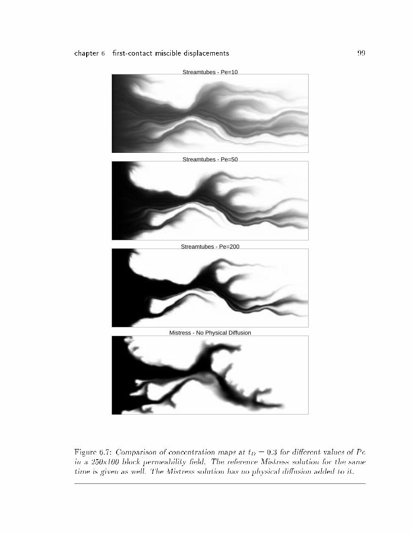
chapter 6 �rst-contact miscible displacements 99
Streamtubes - Pe=10
Streamtubes - Pe=50
Streamtubes - Pe=200
Mistress - No Physical Diffusion
Figure 6.7: Comparison of concentration maps at tD = 0:3 for di�erent values of Pein a 250x100 block permeability �eld. The reference Mistress solution for the same
time is given as well. The Mistress solution has no physical di�usion added to it.
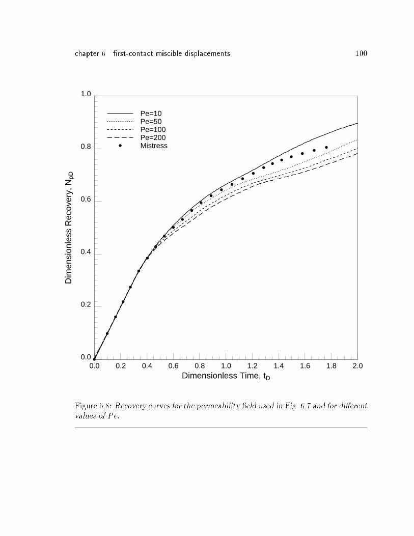
chapter 6 �rst-contact miscible displacements 100
0.0
0.2
0.4
0.6
0.8
1.0
Dim
ensi
onle
ss R
ecov
ery,
NpD
0.0 0.2 0.4 0.6 0.8 1.0 1.2 1.4 1.6 1.8 2.0Dimensionless Time, tD
a
a
a
a
a
a
a
a
a
a
a
a
a
a
aa
aa
aa
aa
aa
aa
Pe=10Pe=50Pe=100Pe=200Mistress
Figure 6.8: Recovery curves for the permeability �eld used in Fig. 6.7 and for di�erentvalues of Pe.
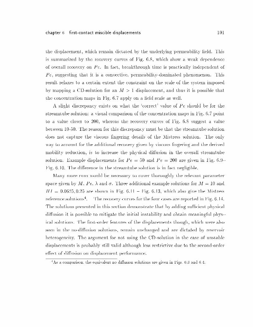
chapter 6 �rst-contact miscible displacements 101
the displacement, which remain dictated by the underlying permeability �eld. This
is summarized by the recovery curves of Fig. 6.8, which show a weak dependence
of overall recovery on Pe. In fact, breakthrough time is practically independent of
Pe, suggesting that it is a convective, permeability-dominated phenomenon. This
result relaxes to a certain extent the constraint on the scale of the system imposed
by mapping a CD-solution for an M > 1 displacement, and thus it is possible that
the concentration maps in Fig. 6.7 apply on a �eld scale as well.
A slight discrepancy exists on what the `correct' value of Pe should be for the
streamtube solution: a visual comparison of the concentration maps in Fig. 6.7 point
to a value closer to 200, whereas the recovery curves of Fig. 6.8 suggest a value
between 10-50. The reason for this discrepancy must be that the streamtube solution
does not capture the viscous �ngering details of the Mistress solution. The only
way to account for the additional recovery given by viscous �ngering and the derived
mobility reduction, is to increase the physical di�usion in the overall streamtube
solution. Example displacements for Pe = 50 and Pe = 200 are given in Fig. 6.9-
Fig. 6.10. The di�erence in the streamtube solution is in fact negligible.
Many more runs would be necessary to cover thoroughly the relevant parameter
space given by M , Pe, � and �. Three additional example solutions for M = 10 and
HI = 0:0625; 0:25 are shown in Fig. 6.11 { Fig. 6.13, which also give the Mistress
reference solutions4. The recovery curves for the four cases are reported in Fig. 6.14.
The solutions presented in this section demonstrate that by adding su�cient physical
di�usion it is possible to mitigate the initial instability and obtain meaningful phys-
ical solutions. The �rst-order features of the displacements though, which were also
seen in the no-di�usion solutions, remain unchanged and are dictated by reservoir
heterogeneity. The argument for not using the CD-solution in the case of unstable
displacements is probably still valid although less restrictive due to the second-order
e�ect of di�usion on displacement performance.
4As a comparison, the equivalent no-di�usion solutions are given in Figs. 6.3 and 6.4.
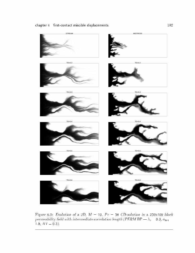
chapter 6 �rst-contact miscible displacements 102
STREAM
TD=0.2
TD=0.3
TD=0.4
TD=0.5
TD=0.6
MISTRESS
TD=0.2
TD=0.3
TD=0.4
TD=0.5
TD=0.6
Figure 6.9: Evolution of a 2D, M = 10, Pe = 50 CD-solution in a 250x100 block
permeability �eld with intermediate correlation length (PERM BP| �c = 0.3, �lnk =1:0, HI = 0:3).
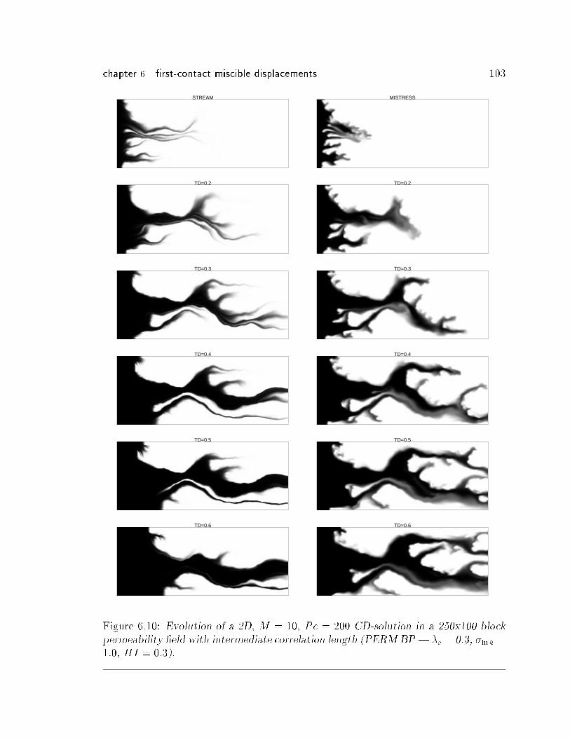
chapter 6 �rst-contact miscible displacements 103
STREAM
TD=0.2
TD=0.3
TD=0.4
TD=0.5
TD=0.6
MISTRESS
TD=0.2
TD=0.3
TD=0.4
TD=0.5
TD=0.6
Figure 6.10: Evolution of a 2D, M = 10, Pe = 200 CD-solution in a 250x100 block
permeability �eld with intermediate correlation length (PERM BP| �c = 0.3, �lnk =1:0, HI = 0:3).
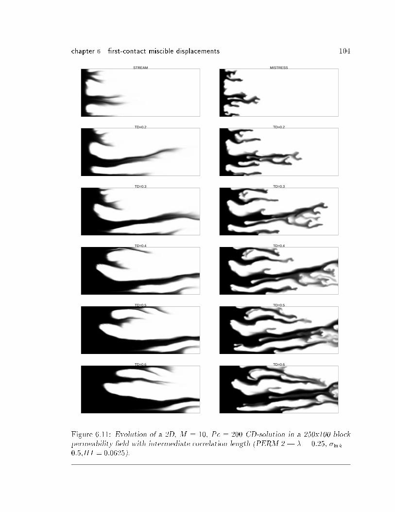
chapter 6 �rst-contact miscible displacements 104
STREAM
TD=0.2
TD=0.3
TD=0.4
TD=0.5
TD=0.6
MISTRESS
TD=0.2
TD=0.3
TD=0.4
TD=0.5
TD=0.6
Figure 6.11: Evolution of a 2D, M = 10, Pe = 200 CD-solution in a 250x100 block
permeability �eld with intermediate correlation length (PERM 2 | � = 0:25, �lnk =0:5,HI = 0:0625).
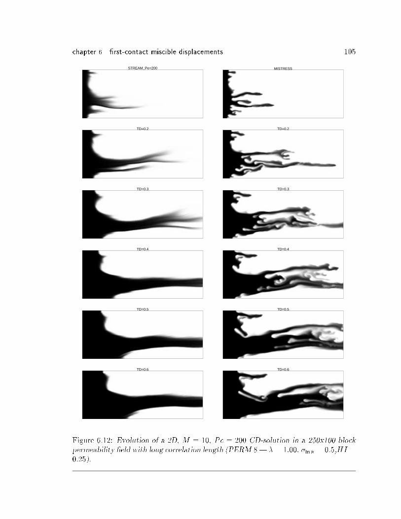
chapter 6 �rst-contact miscible displacements 105
STREAM_Pe=200
TD=0.2
TD=0.3
TD=0.4
TD=0.5
TD=0.6
MISTRESS
TD=0.2
TD=0.3
TD=0.4
TD=0.5
TD=0.6
Figure 6.12: Evolution of a 2D, M = 10, Pe = 200 CD-solution in a 250x100 block
permeability �eld with long correlation length (PERM 8| � = 1:00, �ln k = 0:5,HI =0:25).
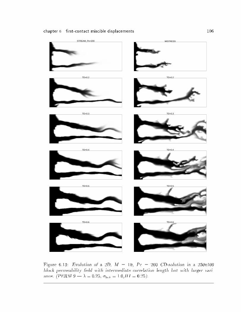
chapter 6 �rst-contact miscible displacements 106
STREAM_Pe=200
TD=0.2
TD=0.3
TD=0.4
TD=0.5
TD=0.6
MISTRESS
TD=0.2
TD=0.3
TD=0.4
TD=0.5
TD=0.6
Figure 6.13: Evolution of a 2D, M = 10, Pe = 200 CD-solution in a 250x100
block permeability �eld with intermediate correlation length but with larger vari-
ance. (PERM 9 | � = 0:25, �ln k = 1:0,HI = 0:25).
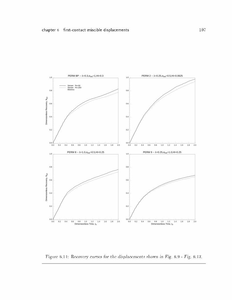
chapter 6 �rst-contact miscible displacements 107
0.0
0.2
0.4
0.6
0.8
1.0
Dim
ensi
onle
ss R
ecov
ery,
NpD
0.0 0.2 0.4 0.6 0.8 1.0 1.2 1.4 1.6 1.8 2.0
PERM BP -- λ=0.3,σlnK=1,HI=0.3
Stream Pe=50Stream Pe=200Mistress
0.0
0.2
0.4
0.6
0.8
1.0
0.0 0.2 0.4 0.6 0.8 1.0 1.2 1.4 1.6 1.8 2.0
PERM 2 -- λ=0.25,σlnK=0.5,HI=0.0625
0.0
0.2
0.4
0.6
0.8
1.0
Dim
ensi
onle
ss R
ecov
ery,
NpD
0.0 0.2 0.4 0.6 0.8 1.0 1.2 1.4 1.6 1.8 2.0Dimensionless Time, tD
PERM 8 -- λ=1.0,σlnK=0.5,HI=0.25
0.0
0.2
0.4
0.6
0.8
1.0
0.0 0.2 0.4 0.6 0.8 1.0 1.2 1.4 1.6 1.8 2.0Dimensionless Time, tD
PERM 9 -- λ=0.25,σlnK=1.0,HI=0.25
Figure 6.14: Recovery curves for the displacements shown in Fig. 6.9 - Fig. 6.13.
chapter 6 �rst-contact miscible displacements 108
6.6 2D Solutions Using Viscous Fingering Model
If the streamtubes are considered to be on a �eld scale, then a one-dimensional viscous
�ngering solution is probably more appropriate than the convection-di�usion solution
to capture the �rst contact miscible displacement of the resident oil. In other words,
each streamtube is considered large enough and homogeneous enough to reach a
Fickian limit for M = 1 and to generate a viscous �ngering ow regime for M > 1.
The e�ective `mixing' zone now grows linearly with time, allowing the instability to
be mitigated even more than in the convection-di�usion approach.
In generating a two-dimensional solutions using the Todd{Longsta� model, a value
for ! must be chosen. An ! � 2=3 is widely used and has been found to match both,
experimental and numerical displacements through homogeneous media (Todd and
Longsta� 1972, Fayers et al. 1992). If the Todd{Longsta� model is made to match
Koval's model then ! becomes a (weak) function of end-point mobility ratio as given
by Eq. 6.16, since Koval's model assumes a �xed solvent concentration of 0.22 to �nd
the mixture viscosity using the quarter power mixing rule. It is unreasonable to be-
lieve that a constant value for ! is able to match all secondary miscible displacements
in homogeneous media, and therefore some functional dependence on M is probably
desired. On the other hand, given the physical limits of ! = 1 (no mixing) and ! = 0
(complete mixing), the large uncertainties in the input data, and the general nonlin-
earity of the problem, it is unlikely that a dependence of ! on M can actually be
detected with the desired degree of accuracy by numerical or laboratory experiments.
To quantify the sensitivity of the streamtube solution on !, the same M = 10
displacement through a 125x50 block heterogeneous system was simulated using in-
cremental values of !, starting from ! = 0 up to ! = 1, with �! = 0:1. Example
concentration maps at tD = 0:3 are shown in Fig. 6.15 and the recovery curves are
shown in Fig. 6.16. The particularly interesting feature of the recovery curves is that
they are not monotonic as a function of !. Recovery increases starting from ! = 0,
reaches a maximum at around ! = 0:6 - 0:7, and then decreases again as it tends to
! = 1:0. It is di�cult to make any general statements about why recovery reaches a
maximum in the range of ! = 0:6 - 0:7, and particularly if it is simply a coincidence
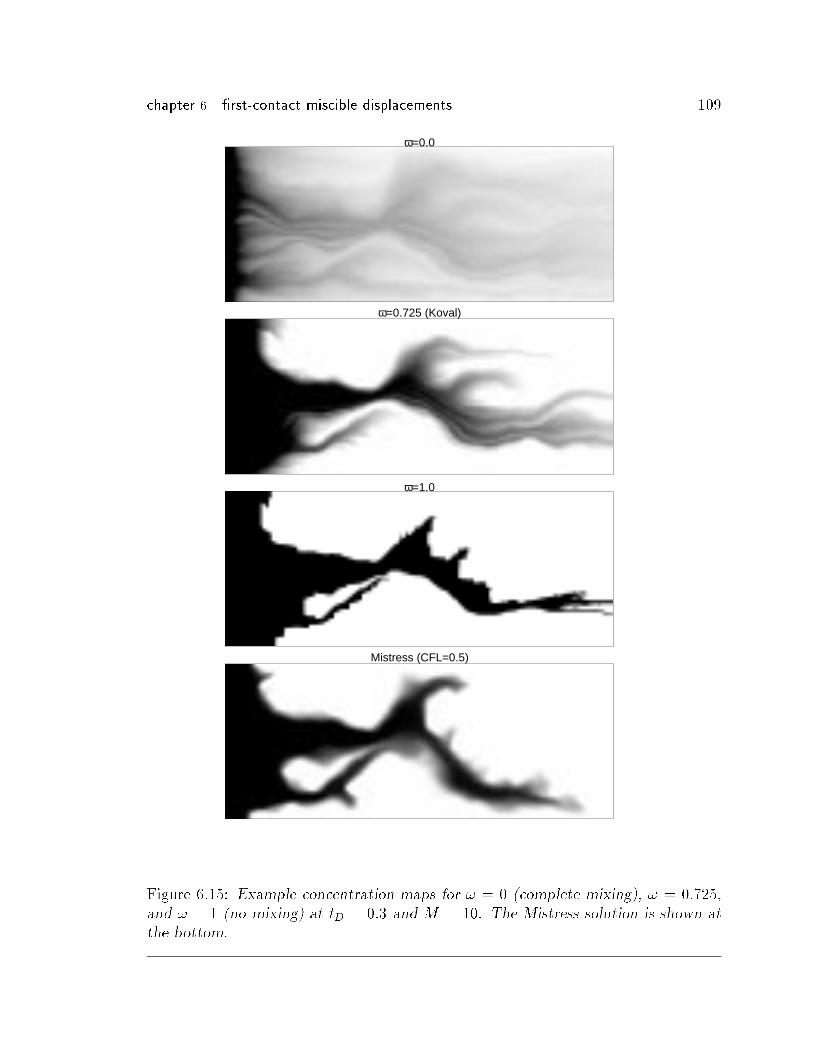
chapter 6 �rst-contact miscible displacements 109
ω=0.0
ω=0.725 (Koval)
ω=1.0
Mistress (CFL=0.5)
Figure 6.15: Example concentration maps for ! = 0 (complete mixing), ! = 0:725,and ! = 1 (no mixing) at tD = 0:3 and M = 10. The Mistress solution is shown at
the bottom.
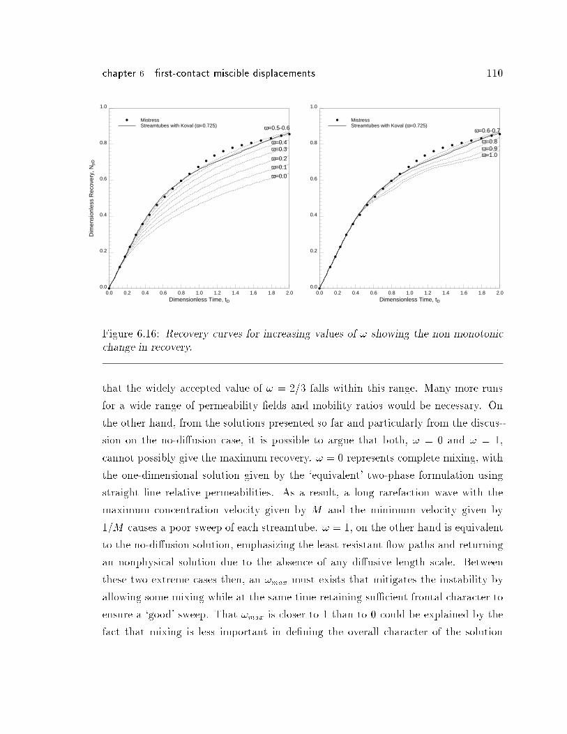
chapter 6 �rst-contact miscible displacements 110
0.0
0.2
0.4
0.6
0.8
1.0
Dim
ensi
onle
ss R
ecov
ery,
NpD
0.0 0.2 0.4 0.6 0.8 1.0 1.2 1.4 1.6 1.8 2.0Dimensionless Time, tD
a
a
a
a
a
a
a
a
a
a
a
a
a
a
aa
aa
aa
aa a
a MistressStreamtubes with Koval (ω=0.725)
ω=0.0
ω=0.1
ω=0.2
ω=0.3ω=0.4
ω=0.5-0.6
0.0
0.2
0.4
0.6
0.8
1.0
0.0 0.2 0.4 0.6 0.8 1.0 1.2 1.4 1.6 1.8 2.0Dimensionless Time, tD
a
a
a
a
a
a
a
a
a
a
a
a
a
a
aa
aa
aa
aa a
a MistressStreamtubes with Koval (ω=0.725)
ω=0.6-0.7
ω=1.0ω=0.9ω=0.8
Figure 6.16: Recovery curves for increasing values of ! showing the non-monotonicchange in recovery.
that the widely accepted value of ! = 2=3 falls within this range. Many more runs
for a wide range of permeability �elds and mobility ratios would be necessary. On
the other hand, from the solutions presented so far and particularly from the discus-
sion on the no-di�usion case, it is possible to argue that both, ! = 0 and ! = 1,
cannot possibly give the maximum recovery. ! = 0 represents complete mixing, with
the one-dimensional solution given by the `equivalent' two-phase formulation using
straight line relative permeabilities. As a result, a long rarefaction wave with the
maximum concentration velocity given by M and the minimum velocity given by
1=M causes a poor sweep of each streamtube. ! = 1, on the other hand is equivalent
to the no-di�usion solution, emphasizing the least resistant ow paths and returning
an nonphysical solution due to the absence of any di�usive length scale. Between
these two extreme cases then, an !max must exists that mitigates the instability by
allowing some mixing while at the same time retaining su�cient frontal character to
ensure a `good' sweep. That !max is closer to 1 than to 0 could be explained by the
fact that mixing is less important in de�ning the overall character of the solution
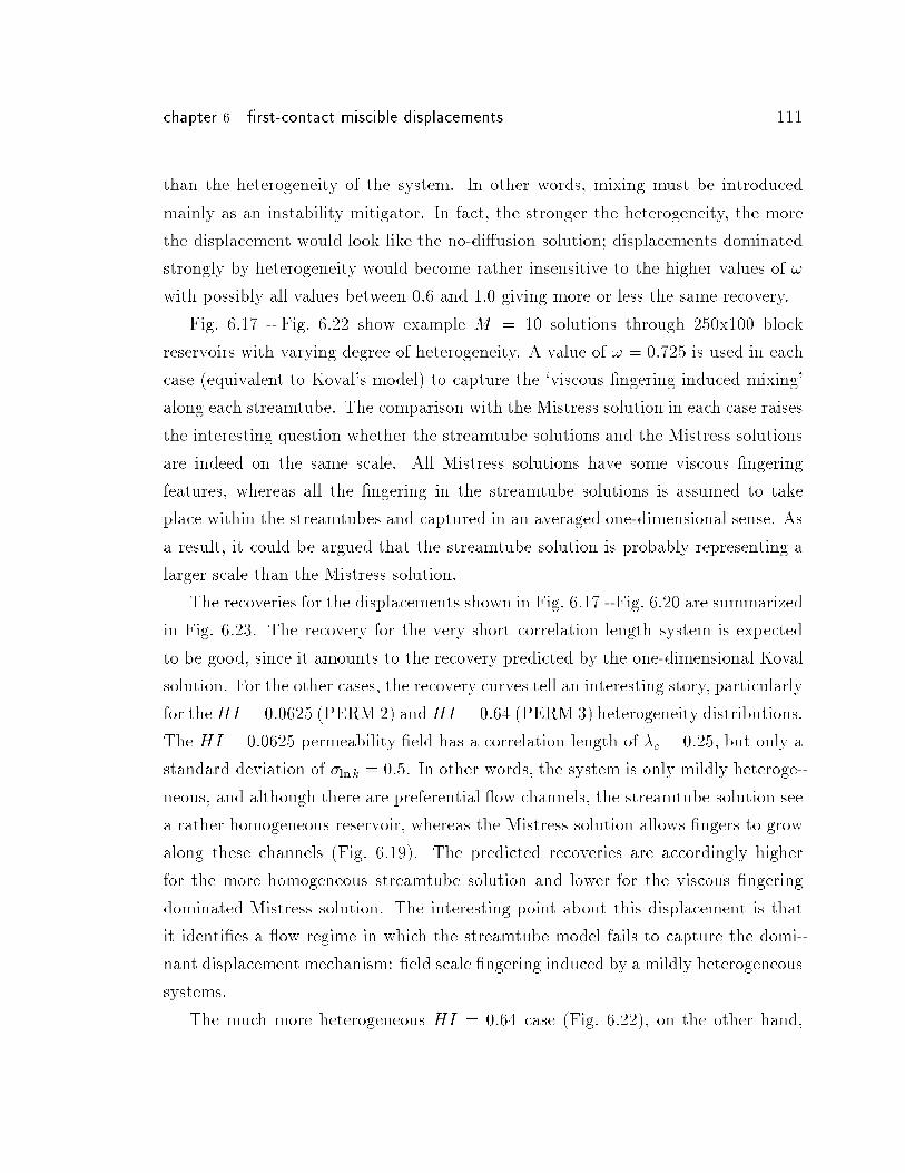
chapter 6 �rst-contact miscible displacements 111
than the heterogeneity of the system. In other words, mixing must be introduced
mainly as an instability mitigator. In fact, the stronger the heterogeneity, the more
the displacement would look like the no-di�usion solution; displacements dominated
strongly by heterogeneity would become rather insensitive to the higher values of !
with possibly all values between 0:6 and 1:0 giving more or less the same recovery.
Fig. 6.17 - Fig. 6.22 show example M = 10 solutions through 250x100 block
reservoirs with varying degree of heterogeneity. A value of ! = 0:725 is used in each
case (equivalent to Koval's model) to capture the `viscous �ngering induced mixing'
along each streamtube. The comparison with the Mistress solution in each case raises
the interesting question whether the streamtube solutions and the Mistress solutions
are indeed on the same scale. All Mistress solutions have some viscous �ngering
features, whereas all the �ngering in the streamtube solutions is assumed to take
place within the streamtubes and captured in an averaged one-dimensional sense. As
a result, it could be argued that the streamtube solution is probably representing a
larger scale than the Mistress solution.
The recoveries for the displacements shown in Fig. 6.17 - Fig. 6.20 are summarized
in Fig. 6.23. The recovery for the very short correlation length system is expected
to be good, since it amounts to the recovery predicted by the one-dimensional Koval
solution. For the other cases, the recovery curves tell an interesting story, particularly
for theHI = 0:0625 (PERM 2) andHI = 0:64 (PERM 3) heterogeneity distributions.
The HI = 0:0625 permeability �eld has a correlation length of �c = 0:25, but only a
standard deviation of �ln k = 0:5. In other words, the system is only mildly heteroge-
neous, and although there are preferential ow channels, the streamtube solution see
a rather homogeneous reservoir, whereas the Mistress solution allows �ngers to grow
along these channels (Fig. 6.19). The predicted recoveries are accordingly higher
for the more homogeneous streamtube solution and lower for the viscous �ngering
dominated Mistress solution. The interesting point about this displacement is that
it identi�es a ow regime in which the streamtube model fails to capture the domi-
nant displacement mechanism: �eld scale �ngering induced by a mildly heterogeneous
systems.
The much more heterogeneous HI = 0:64 case (Fig. 6.22), on the other hand,
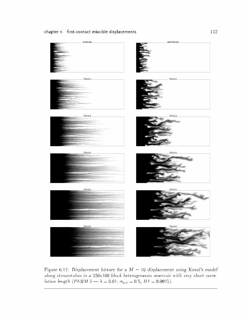
chapter 6 �rst-contact miscible displacements 112
STREAM
TD=0.2
TD=0.3
TD=0.4
TD=0.5
TD=0.6
MISTRESS
TD=0.2
TD=0.3
TD=0.4
TD=0.5
TD=0.6
Figure 6.17: Displacement history for a M = 10 displacement using Koval's model
along streamtubes in a 250x100 block heterogeneous reservoir with very short corre-
lation length (PERM 5 | � = 0:01, �ln k = 0:5, HI = 0:0025).
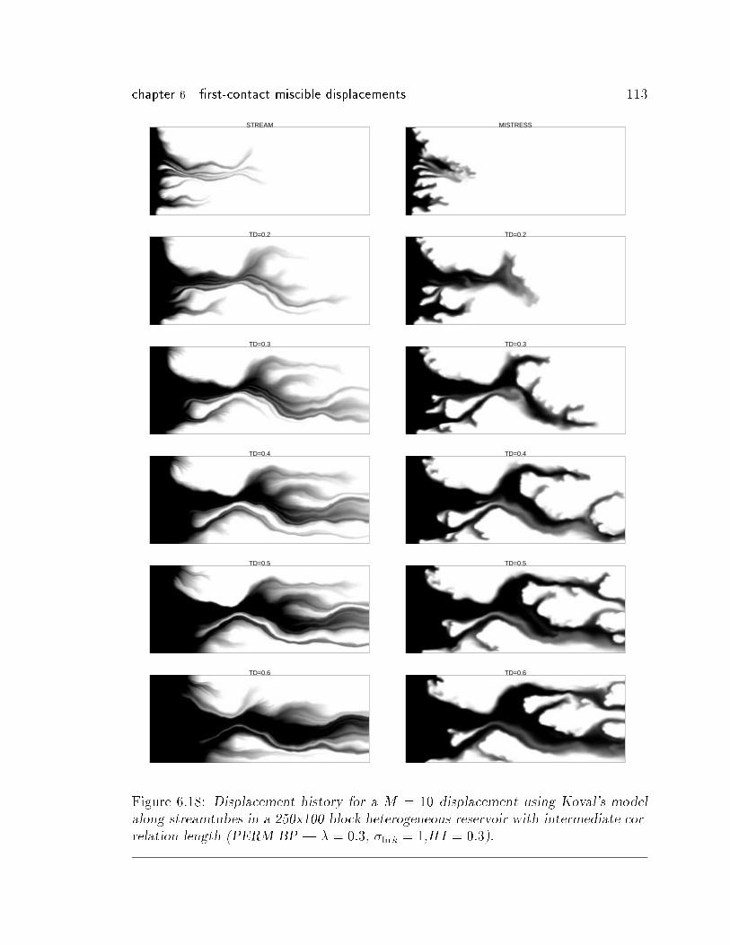
chapter 6 �rst-contact miscible displacements 113
STREAM
TD=0.2
TD=0.3
TD=0.4
TD=0.5
TD=0.6
MISTRESS
TD=0.2
TD=0.3
TD=0.4
TD=0.5
TD=0.6
Figure 6.18: Displacement history for a M = 10 displacement using Koval's model
along streamtubes in a 250x100 block heterogeneous reservoir with intermediate cor-
relation length (PERM BP | � = 0:3, �ln k = 1,HI = 0:3).
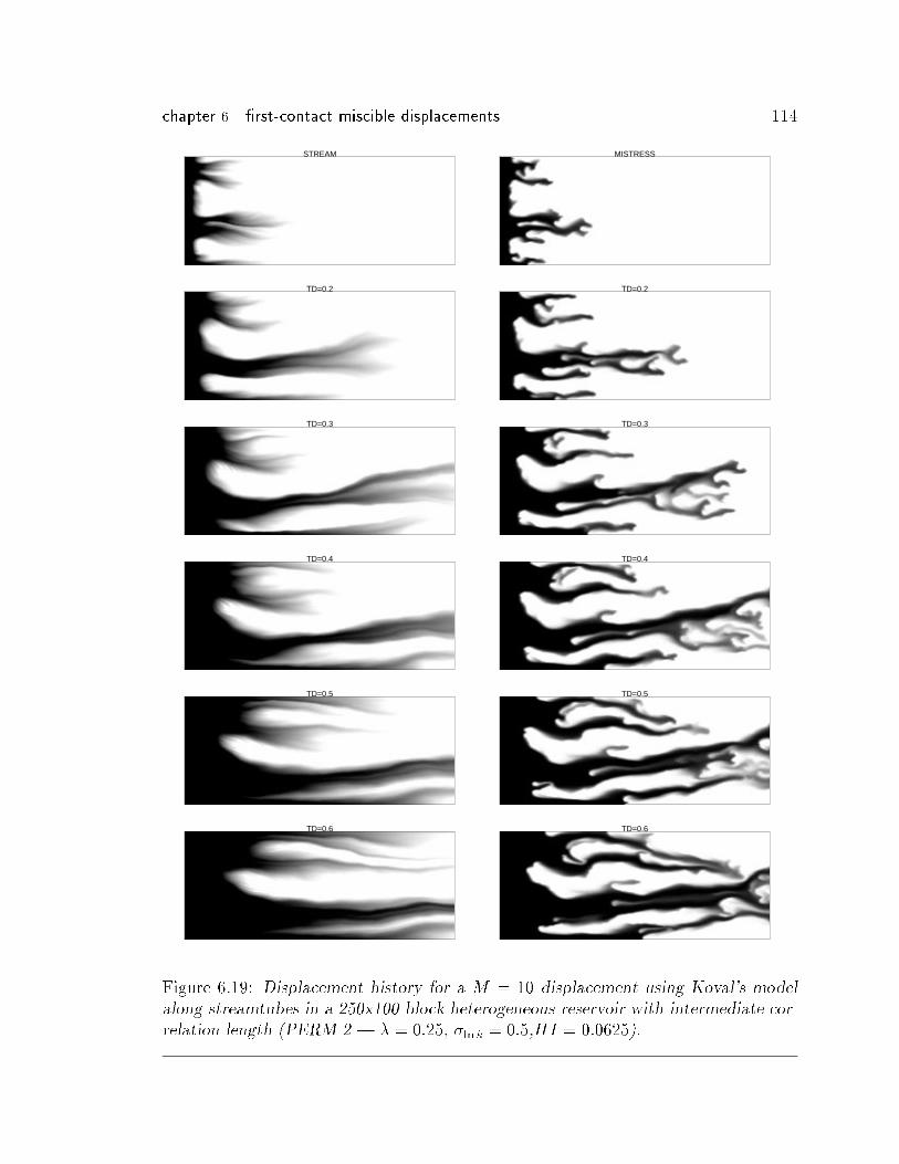
chapter 6 �rst-contact miscible displacements 114
STREAM
TD=0.2
TD=0.3
TD=0.4
TD=0.5
TD=0.6
MISTRESS
TD=0.2
TD=0.3
TD=0.4
TD=0.5
TD=0.6
Figure 6.19: Displacement history for a M = 10 displacement using Koval's model
along streamtubes in a 250x100 block heterogeneous reservoir with intermediate cor-
relation length (PERM 2 | � = 0:25, �ln k = 0:5,HI = 0:0625).
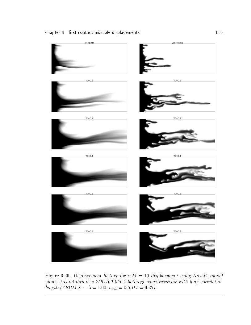
chapter 6 �rst-contact miscible displacements 115
STREAM
TD=0.2
TD=0.3
TD=0.4
TD=0.5
TD=0.6
MISTRESS
TD=0.2
TD=0.3
TD=0.4
TD=0.5
TD=0.6
Figure 6.20: Displacement history for a M = 10 displacement using Koval's model
along streamtubes in a 250x100 block heterogeneous reservoir with long correlation
length (PERM 8 | � = 1:00, �ln k = 0:5,HI = 0:25).
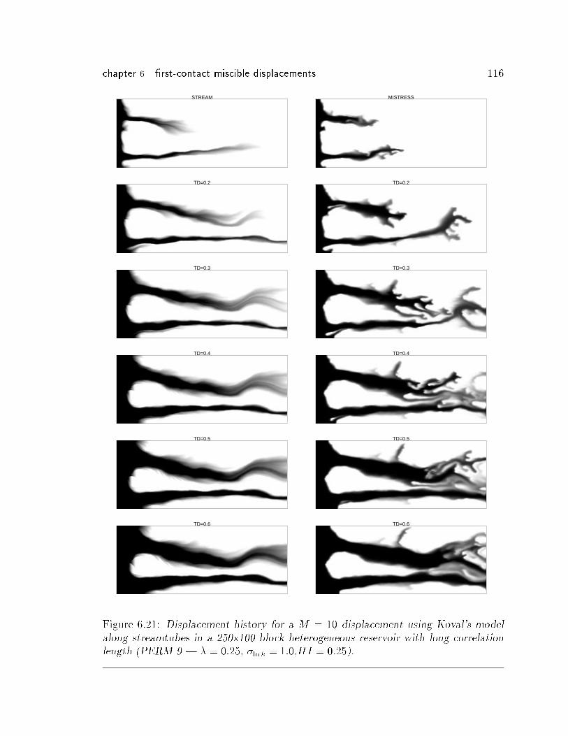
chapter 6 �rst-contact miscible displacements 116
STREAM
TD=0.2
TD=0.3
TD=0.4
TD=0.5
TD=0.6
MISTRESS
TD=0.2
TD=0.3
TD=0.4
TD=0.5
TD=0.6
Figure 6.21: Displacement history for a M = 10 displacement using Koval's model
along streamtubes in a 250x100 block heterogeneous reservoir with long correlation
length (PERM 9 | � = 0:25, �ln k = 1:0,HI = 0:25).
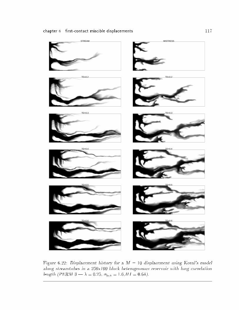
chapter 6 �rst-contact miscible displacements 117
STREAM
TD=0.2
TD=0.3
TD=0.4
TD=0.5
TD=0.6
MISTRESS
TD=0.2
TD=0.3
TD=0.4
TD=0.5
TD=0.6
Figure 6.22: Displacement history for a M = 10 displacement using Koval's model
along streamtubes in a 250x100 block heterogeneous reservoir with long correlation
length (PERM 3 | � = 0:25, �ln k = 1:6,HI = 0:64).
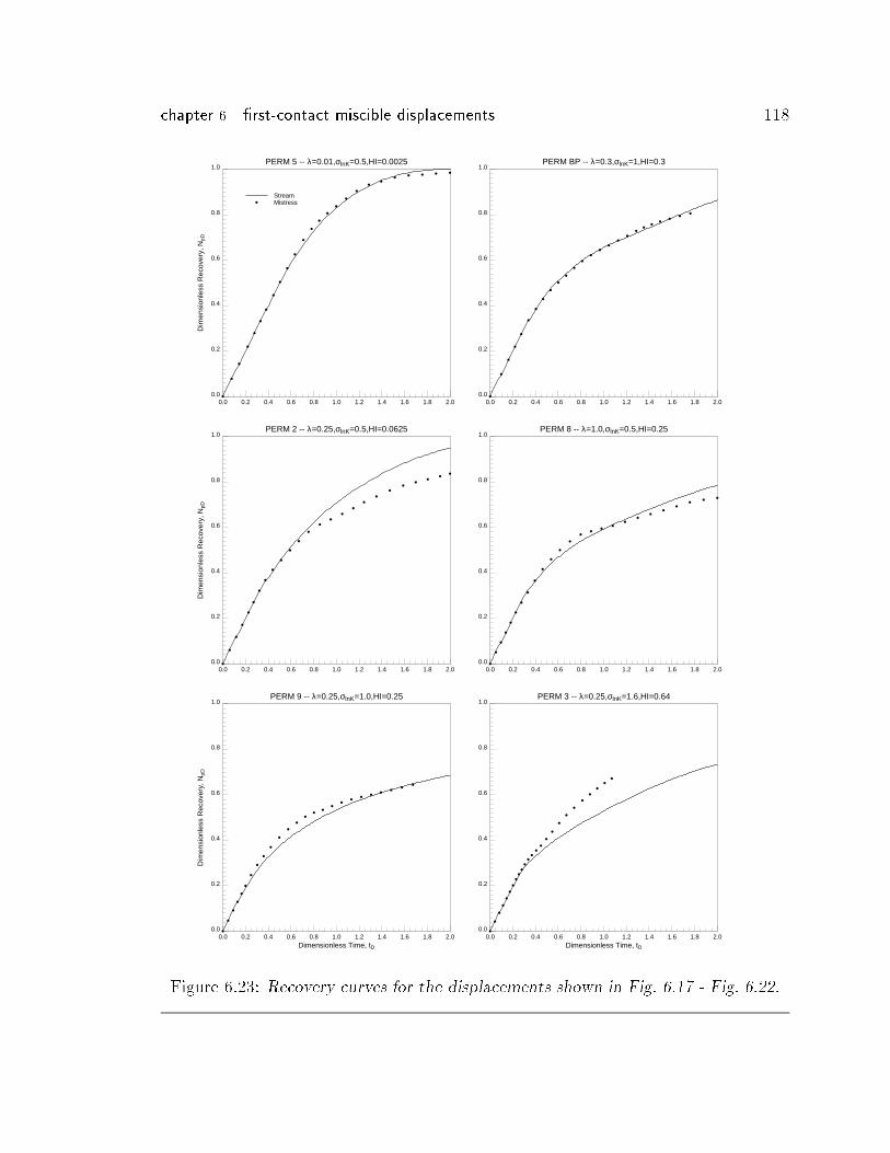
chapter 6 �rst-contact miscible displacements 118
0.0
0.2
0.4
0.6
0.8
1.0
Dim
ensi
onle
ss R
ecov
ery,
NpD
0.0 0.2 0.4 0.6 0.8 1.0 1.2 1.4 1.6 1.8 2.0
PERM 5 -- λ=0.01,σlnK=0.5,HI=0.0025
a
a
a
a
a
a
a
a
a
a
a
a
a
a
a
a
a
a
aa
aa a a a
aStreamMistress
0.0
0.2
0.4
0.6
0.8
1.0
0.0 0.2 0.4 0.6 0.8 1.0 1.2 1.4 1.6 1.8 2.0
PERM BP -- λ=0.3,σlnK=1,HI=0.3
a
a
a
a
a
a
a
a
a
a
a
a
a
a
aa
aa
aa
aa
aa
a
0.0
0.2
0.4
0.6
0.8
1.0
Dim
ensi
onle
ss R
ecov
ery,
NpD
0.0 0.2 0.4 0.6 0.8 1.0 1.2 1.4 1.6 1.8 2.0
PERM 2 -- λ=0.25,σlnK=0.5,HI=0.0625
a
a
a
a
a
a
a
a
a
a
a
a
a
a
a
a
a
a
a
aa
aa
aa
0.0
0.2
0.4
0.6
0.8
1.0
0.0 0.2 0.4 0.6 0.8 1.0 1.2 1.4 1.6 1.8 2.0
PERM 8 -- λ=1.0,σlnK=0.5,HI=0.25
a
a
a
a
a
a
a
a
a
a
a
a
a
aa
aa
aa
aa
aa
a a
0.0
0.2
0.4
0.6
0.8
1.0
Dim
ensi
onle
ss R
ecov
ery,
NpD
0.0 0.2 0.4 0.6 0.8 1.0 1.2 1.4 1.6 1.8 2.0Dimensionless Time, tD
PERM 9 -- λ=0.25,σlnK=1.0,HI=0.25
a
a
a
a
a
a
a
a
a
a
a
a
a
aa
aa
aa
aa
aa
aa
0.0
0.2
0.4
0.6
0.8
1.0
0.0 0.2 0.4 0.6 0.8 1.0 1.2 1.4 1.6 1.8 2.0Dimensionless Time, tD
PERM 3 -- λ=0.25,σlnK=1.6,HI=0.64
a
a
a
a
a
a
a
a
aa
a
aaaa
a
a
a
a
a
a
a
a
aa
Figure 6.23: Recovery curves for the displacements shown in Fig. 6.17 - Fig. 6.22.
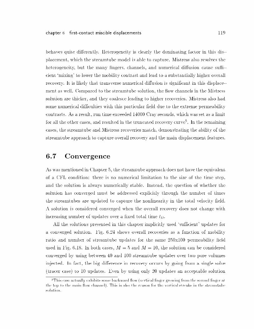
chapter 6 �rst-contact miscible displacements 119
behaves quite di�erently. Heterogeneity is clearly the dominating factor in this dis-
placement, which the streamtube model is able to capture. Mistress also resolves the
heterogeneity, but the many �ngers, channels, and numerical di�usion cause su�-
cient `mixing' to lower the mobility contrast and lead to a substantially higher overall
recovery. It is likely that transverse numerical di�usion is signi�cant in this displace-
ment as well. Compared to the streamtube solution, the ow channels in the Mistress
solution are thicker, and they coalesce leading to higher recoveries. Mistress also had
some numerical di�culties with this particular �eld due to the extreme permeability
contrasts. As a result, run time exceeded 14000 Cray seconds, which was set as a limit
for all the other cases, and resulted in the truncated recovery curve5. In the remaining
cases, the streamtube and Mistress recoveries match, demonstrating the ability of the
streamtube approach to capture overall recovery and the main displacement features.
6.7 Convergence
As was mentioned in Chapter 5, the streamtube approach does not have the equivalent
of a CFL condition: there is no numerical limitation to the size of the time step,
and the solution is always numerically stable. Instead, the question of whether the
solution has converged must be addressed explicitly through the number of times
the streamtubes are updated to capture the nonlinearity in the total velocity �eld.
A solution is considered converged when the overall recovery does not change with
increasing number of updates over a �xed total time tD.
All the solutions presented in this chapter implicitly used `su�cient' updates for
a converged solution. Fig. 6.24 shows overall recoveries as a function of mobility
ratio and number of streamtube updates for the same 250x100 permeability �eld
used in Fig. 6.18. In both cases, M = 5 and M = 10, the solution can be considered
converged by using between 40 and 100 streamtube updates over two pore volumes
injected. In fact, the big di�erence in recovery occurs by going from a single solve
(tracer case) to 10 updates. Even by using only 20 updates an acceptable solution
5This case actually exhibits some backward ow (vertical �nger growing from the second �nger atthe top to the main ow channel). This is also the reason for the vertical streaks in the streamtubesolution.
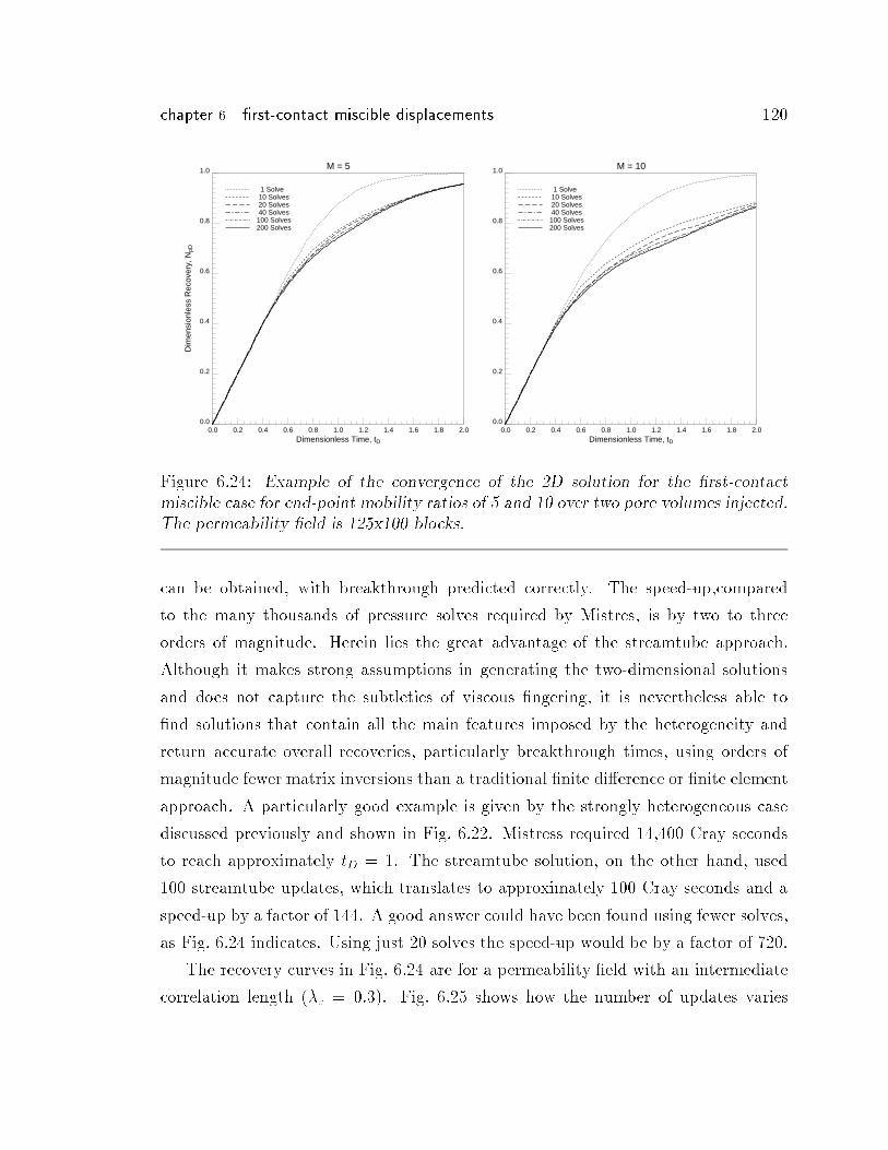
chapter 6 �rst-contact miscible displacements 120
0.0
0.2
0.4
0.6
0.8
1.0
Dim
ensi
onle
ss R
ecov
ery,
NpD
0.0 0.2 0.4 0.6 0.8 1.0 1.2 1.4 1.6 1.8 2.0Dimensionless Time, tD
M = 5
1 Solve 10 Solves 20 Solves 40 Solves100 Solves200 Solves
0.0
0.2
0.4
0.6
0.8
1.0
0.0 0.2 0.4 0.6 0.8 1.0 1.2 1.4 1.6 1.8 2.0Dimensionless Time, tD
M = 10
1 Solve 10 Solves 20 Solves 40 Solves100 Solves200 Solves
Figure 6.24: Example of the convergence of the 2D solution for the �rst-contactmiscible case for end-point mobility ratios of 5 and 10 over two pore volumes injected.The permeability �eld is 125x100 blocks.
can be obtained, with breakthrough predicted correctly. The speed-up,compared
to the many thousands of pressure solves required by Mistres, is by two to three
orders of magnitude. Herein lies the great advantage of the streamtube approach.
Although it makes strong assumptions in generating the two-dimensional solutions
and does not capture the subtleties of viscous �ngering, it is nevertheless able to
�nd solutions that contain all the main features imposed by the heterogeneity and
return accurate overall recoveries, particularly breakthrough times, using orders of
magnitude fewer matrix inversions than a traditional �nite di�erence or �nite element
approach. A particularly good example is given by the strongly heterogeneous case
discussed previously and shown in Fig. 6.22. Mistress required 14,400 Cray seconds
to reach approximately tD = 1. The streamtube solution, on the other hand, used
100 streamtube updates, which translates to approximately 100 Cray seconds and a
speed-up by a factor of 144. A good answer could have been found using fewer solves,
as Fig. 6.24 indicates. Using just 20 solves the speed-up would be by a factor of 720.
The recovery curves in Fig. 6.24 are for a permeability �eld with an intermediate
correlation length (�c = 0:3). Fig. 6.25 shows how the number of updates varies
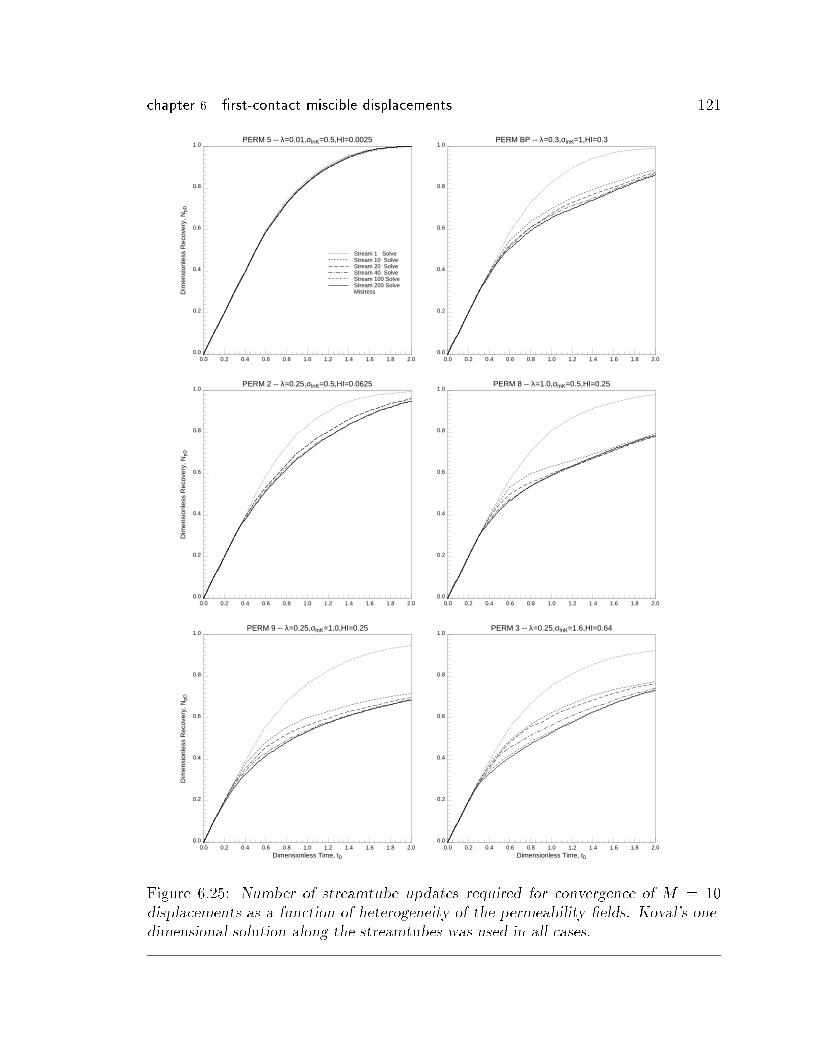
chapter 6 �rst-contact miscible displacements 121
0.0
0.2
0.4
0.6
0.8
1.0
Dim
ensi
onle
ss R
ecov
ery,
NpD
0.0 0.2 0.4 0.6 0.8 1.0 1.2 1.4 1.6 1.8 2.0
PERM 5 -- λ=0.01,σlnK=0.5,HI=0.0025
Stream 1 SolveStream 10 SolveStream 20 SolveStream 40 SolveStream 100 SolveStream 200 SolveMistress
0.0
0.2
0.4
0.6
0.8
1.0
0.0 0.2 0.4 0.6 0.8 1.0 1.2 1.4 1.6 1.8 2.0
PERM BP -- λ=0.3,σlnK=1,HI=0.3
0.0
0.2
0.4
0.6
0.8
1.0
Dim
ensi
onle
ss R
ecov
ery,
NpD
0.0 0.2 0.4 0.6 0.8 1.0 1.2 1.4 1.6 1.8 2.0
PERM 2 -- λ=0.25,σlnK=0.5,HI=0.0625
0.0
0.2
0.4
0.6
0.8
1.0
0.0 0.2 0.4 0.6 0.8 1.0 1.2 1.4 1.6 1.8 2.0
PERM 8 -- λ=1.0,σlnK=0.5,HI=0.25
0.0
0.2
0.4
0.6
0.8
1.0
Dim
ensi
onle
ss R
ecov
ery,
NpD
0.0 0.2 0.4 0.6 0.8 1.0 1.2 1.4 1.6 1.8 2.0Dimensionless Time, tD
PERM 9 -- λ=0.25,σlnK=1.0,HI=0.25
0.0
0.2
0.4
0.6
0.8
1.0
0.0 0.2 0.4 0.6 0.8 1.0 1.2 1.4 1.6 1.8 2.0Dimensionless Time, tD
PERM 3 -- λ=0.25,σlnK=1.6,HI=0.64
Figure 6.25: Number of streamtube updates required for convergence of M = 10displacements as a function of heterogeneity of the permeability �elds. Koval's one-
dimensional solution along the streamtubes was used in all cases.
chapter 6 �rst-contact miscible displacements 122
with correlation length and the variability of the permeability �eld. The correla-
tion length is the more important parameter in setting the number of updates to
reach a converged solution. For short correlation lengths, there are no particular ow
paths for the streamtubes to identify. On average, the streamtubes will not see a
major change in their geometry or direction and the recovery is matched because of
the one-dimensional viscous �ngering model along each streamtube. As the correla-
tion length increases, ow paths are created leading to more dramatic changes in the
streamtube geometries. Streamtubes in the high permeability zones will progressively
become thinner whereas streamtubes in the low permeability zones progressively be-
come thicker. In order to capture this progressive change in streamtube geometries,
the streamtubes must be updated more frequently. Nevertheless, in all cases, the
streamtube approach is able to capture overall recoveries requiring approximately
100 solves (or fewer) which represent a speed-up of at least two orders of magnitude
compared to the reference �nite-di�erence solutions presented in this chapter.
6.7.1 The Higgins and Leighton Approach
As in the two-phase immiscible case, an alternative to updating the streamtubes to
capture the nonlinearity of the displacement is to keep the streamtubes �xed and
allocate the ow according to the total ow resistance of each streamtube. Although
the Higgins and Leighton approach gave reasonably good recovery curves in the im-
miscible case, the error in breakthrough time is expected to be more pronounced for
�rst-contact miscible ow due to the stronger nonlinearity of the formulation.
King et al. (1993) modi�ed the Higgins and Leighton's approach and found `boost'
factors for each streamline by calculating the total ow resistance as an integration
from the inlet to the isobar located at the tip of the leading �nger, rather than
using the total length of the streamline from inlet to outlet as required in Eq. 5.12.
King et al. realized that at early times the resistance, Ri, would be dominated by
the unswept part of the streamtube, thus underestimating the nonlinearity of the
displacement. The placement of an isobar at the leading �nger is a clever way to
reduce the in uence of the unswept region on ow resistance, but is also an indication
that the approach of Higgins and Leighton will likely fail for displacements that are
chapter 6 �rst-contact miscible displacements 123
strongly nonlinear. Using the isobar modi�cation may be an alternative though it
clearly has some problems as well. For example, it may be di�cult to pick the `leading'
�nger at early times |in fact, choosing the wrong �nger will cause convergence onto
a wrong solution, because it will force the smallest ow resistance on that particular
�nger and allow it to grow the fastest. The problem might be corrected by using an
isobar that is removed from the leading �nger by some appropriate length (although
that in turn raises the question of how much to remove the isobar from the leading
�nger). It is worth noting that the di�culties found by King et al. were anticipated
by Martin et al. (1973), who found that immiscible displacement with favorable
mobility ratios (i.e. piston-like displacements with a mobility di�erence across the
front) could not be predicted as well unfavorable mobility ratio displacement using
�xed streamtubes.
Fig. 6.26 compares recoveries for six di�erent permeability �elds. Except for the
uncorrelated permeability case, the Higgins and Leighton approach falls between the
single-solve and the converged streamtube solution, underestimating the nonlinear-
ity of the displacement, particularly breakthrough. By how much the Higgins and
Leighton approach will, in general, underestimate the nonlinearity of the displacement
though is hard to quantify, because it will depend strongly on the type of correlated
permeability structure. Furthermore, the Higgins and Leighton method must be used
with caution in light of the inevitable error that is introduced when evaluating the
ow resistances using Eq. 5.12, which is likely to become more signi�cant the stronger
the system heterogeneity. A case in point is the recovery curves for strongly hetero-
geneous permeability �eld (PERM 3) in Fig. 6.26. It is likely that that Higgins and
Leighton solution is seeing a substantial error due to the strong heterogeneity of the
system (see Fig. 6.22). Thus, the conclusion drawn for the immiscible case applies
here as well: given that 40 streamtube updates will generally result in a converged
streamtube solution, the small gain in speed o�ered by the Higgins and Leighton
method does not o�set the error in recovery that may result.
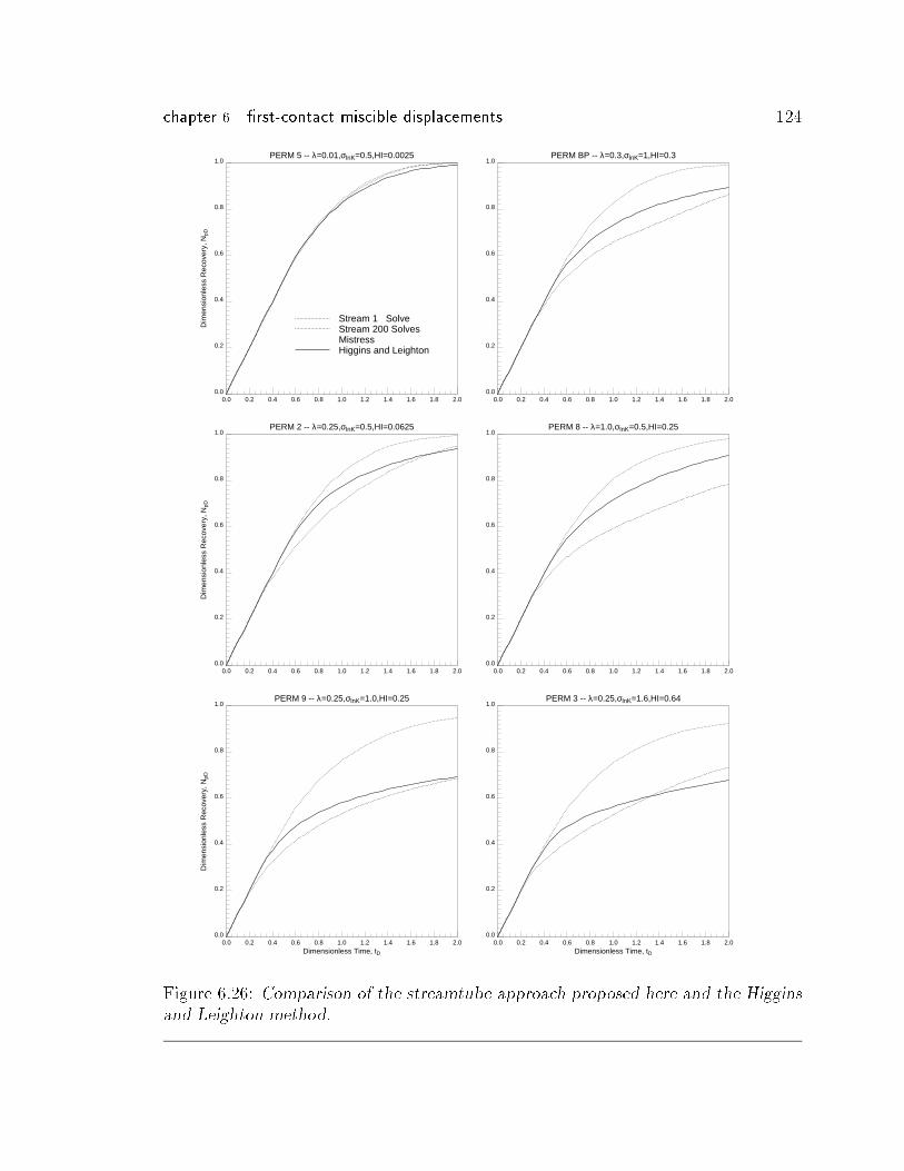
chapter 6 �rst-contact miscible displacements 124
0.0
0.2
0.4
0.6
0.8
1.0
Dim
ensi
onle
ss R
ecov
ery,
NpD
0.0 0.2 0.4 0.6 0.8 1.0 1.2 1.4 1.6 1.8 2.0
PERM 5 -- λ=0.01,σlnK=0.5,HI=0.0025
Stream 1 SolveStream 200 SolvesMistressHiggins and Leighton
0.0
0.2
0.4
0.6
0.8
1.0
0.0 0.2 0.4 0.6 0.8 1.0 1.2 1.4 1.6 1.8 2.0
PERM BP -- λ=0.3,σlnK=1,HI=0.3
0.0
0.2
0.4
0.6
0.8
1.0
Dim
ensi
onle
ss R
ecov
ery,
NpD
0.0 0.2 0.4 0.6 0.8 1.0 1.2 1.4 1.6 1.8 2.0
PERM 2 -- λ=0.25,σlnK=0.5,HI=0.0625
0.0
0.2
0.4
0.6
0.8
1.0
0.0 0.2 0.4 0.6 0.8 1.0 1.2 1.4 1.6 1.8 2.0
PERM 8 -- λ=1.0,σlnK=0.5,HI=0.25
0.0
0.2
0.4
0.6
0.8
1.0
Dim
ensi
onle
ss R
ecov
ery,
NpD
0.0 0.2 0.4 0.6 0.8 1.0 1.2 1.4 1.6 1.8 2.0Dimensionless Time, tD
PERM 9 -- λ=0.25,σlnK=1.0,HI=0.25
0.0
0.2
0.4
0.6
0.8
1.0
0.0 0.2 0.4 0.6 0.8 1.0 1.2 1.4 1.6 1.8 2.0Dimensionless Time, tD
PERM 3 -- λ=0.25,σlnK=1.6,HI=0.64
Figure 6.26: Comparison of the streamtube approach proposed here and the Higgins
and Leighton method.
chapter 6 �rst-contact miscible displacements 125
6.8 Applications
The real power of the streamtube approach lies in its ability to produce solutions
that capture the main features imposed by the underlying permeability �eld while
using orders of magnitude less CPU time than traditional simulation techniques. Its
strength is not in resolving the details of the displacements, although the control on
numerical di�usion may suggest it, but in being able to produce reasonably accurate
recoveries very quickly. As such, it is ideally suited for a statistical approach to reser-
voir forecasting. A large number of statistically identical permeability realizations can
be processed to generate a spread in recovery for a particular combination of reservoir
geology and displacement mechanism. The streamtube approach may also be used as
a �lter: the permeability �elds that returned the maximum and minimum recoveries
can be singled out and used in a much more expensive �nite-di�erence simulation to
con�rm the uncertainty.
The speed of the streamtube approach can be used in many ways, but becomes
particularly appealing when a parameter space of interest includes reservoir hetero-
geneity, in which case many simulations are required to obtain a statistically meaning-
ful answer. An example of a parameter space that has received considerable attention
recently (Tchelepi 1994, Araktingi and Orr 1993, Waggoner et. al 1992, Sorbie et. al
1992) has been in the area of unstable displacements through heterogeneous systems.
In its most simple representation, the parameter space is given by the end-point mo-
bility ratio (instability) and heterogeneity index HI (heterogeneity), although HI is
clearly an incomplete parameter for quantifying the complex geologic structure of a
real reservoir. Nevertheless, HI can give some indication of the degree of heterogene-
ity of the reservoir, particularly if it is used in a statistical sense. A partial sweep
of the parameter space is shown in Fig. 6.27. There are 30 recovery curves for each
of the six M -HI pairs. Mobility ratio increases from left to right and heterogeneity
increases from top to bottom. All underlying permeability �elds have 125x50 grid
blocks.
Fig. 6.27 quanti�es how nonlinearity in the velocity �eld and heterogeneity inter-
act, but does so statistically, rather than using a single recovery for each case. As
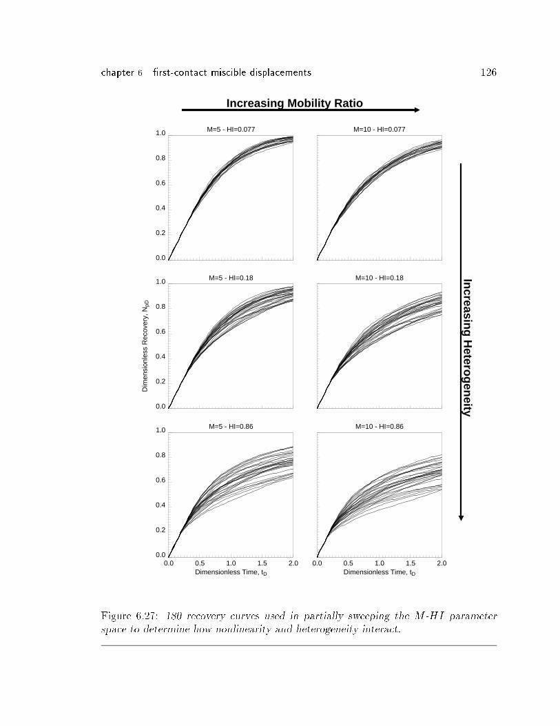
chapter 6 �rst-contact miscible displacements 126
0.0
0.2
0.4
0.6
0.8
1.0
M=5 - HI=0.077
M=10 - HI=0.077
0.0
0.2
0.4
0.6
0.8
1.0
Dim
ensi
onle
ss R
ecov
ery,
NpD
M=5 - HI=0.18
M=10 - HI=0.18
0.0
0.2
0.4
0.6
0.8
1.0
0.0 0.5 1.0 1.5 2.0Dimensionless Time, tD
M=5 - HI=0.86
0.0 0.5 1.0 1.5 2.0Dimensionless Time, tD
M=10 - HI=0.86
Increasing Mobility RatioIn
creasing
Hetero
gen
eity
Figure 6.27: 180 recovery curves used in partially sweeping the M -HI parameter
space to determine how nonlinearity and heterogeneity interact.
chapter 6 �rst-contact miscible displacements 127
a result, the weakness of HI as a parameter is traded for a more convincing spread
in recovery given by the 30 curves for each case. Some interesting observations may
be made from Fig. 6.27: (1) nonlinearity and reservoir heterogeneity interact to cre-
ate a spread in recovery that increases with increasing mobility ratio and increasing
heterogeneity; (2) of the two parameters, heterogeneity is clearly the dominant fac-
tor in establishing recovery, although an increasing mobility ratio causes the spread
between minimum and maximum recovery to increase slightly; (3) the most impor-
tant conclusion to be drawn comes from realizing that the recovery areas partially
overlap from one case to the next. A higher heterogeneity index or mobility ratio
does not automatically lead to lower recoveries compared to a system with lower
heterogeneity or mobility ratio, although on average this conclusion does hold. For
example, an M = 5-HI = 0:86 pair exists that will return a higher recovery then an
M = 10-HI = 0:86 pair.
The 180 recoveries of Fig. 6.28 would have taken a prohibitively long time using
a traditional �nite di�erence approach. Instead, if the streamtube approach is used
as a �lter for the 180 images, the number of solutions required to establish �rmly the
spread in recoveries is just six | two per case | as shown in Fig. 6.28.
6.9 Concluding Remarks
This section demonstrated that the streamtube approach is able to model �rst-contact
miscible displacements in heterogeneous systems using several orders of magnitude
fewer matrix inversions than traditional �nite di�erence solutions. Reservoir hetero-
geneity emerged as the dominant factor in establishing sweep and recovery e�ciency.
Although di�usion or a viscous �ngering model improve on the instabilities inherent
in the Riemann approach, they do not change the �rst-order displacement features
imposed by the underlying permeability �eld. This also holds for all the Mistress
solutions presented as comparisons. Thus, the main conclusion to be drawn from this
chapter is that it may be su�cient to capture the �eld scale reservoir heterogeneity
structure to obtain a good �rst order estimate of recovery, even in strongly nonlin-
ear displacements. The variation in recovery due to a speci�c choice of permeability
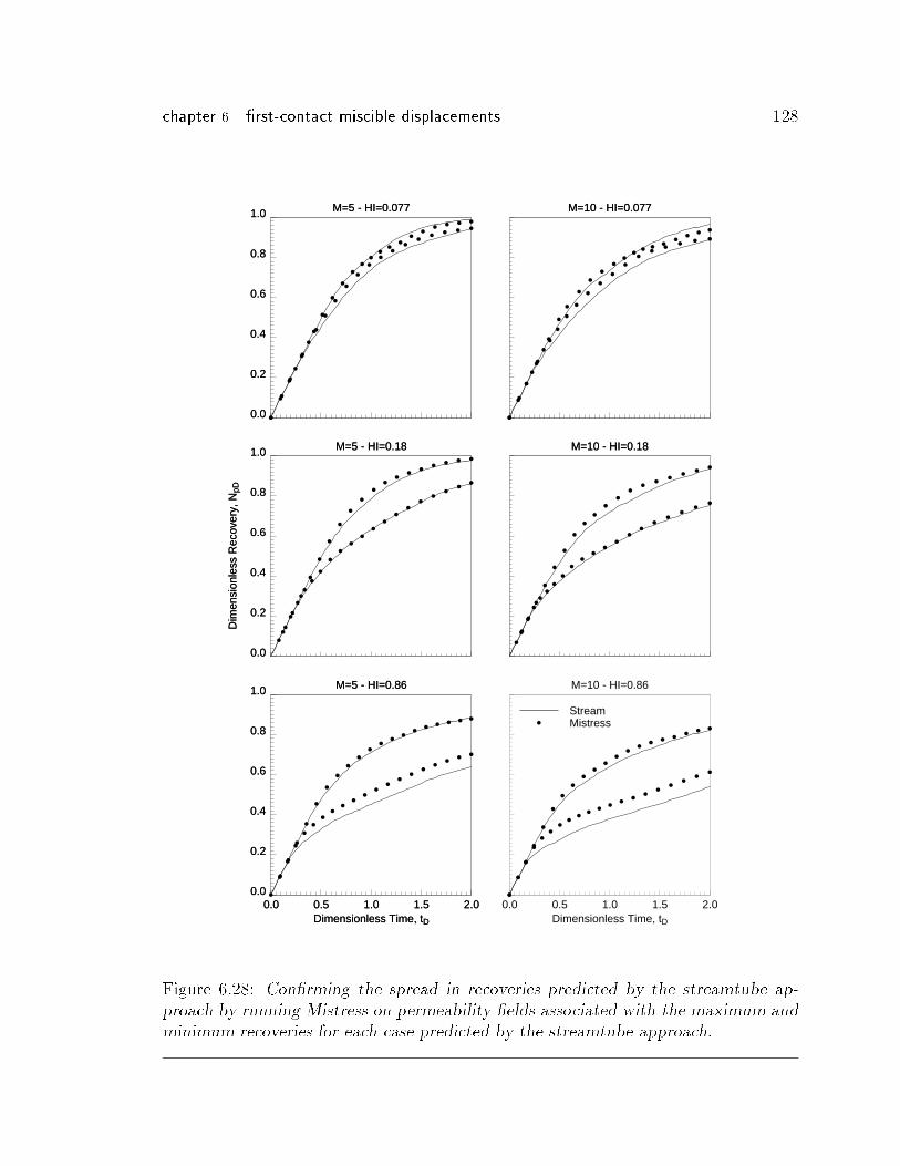
chapter 6 �rst-contact miscible displacements 128
0.0
0.2
0.4
0.6
0.8
1.0
M=5 - HI=0.077
0.0
0.2
0.4
0.6
0.8
1.0
M=5 - HI=0.077
a
a
a
a
a
a
a
a
aaaaaaa
aa a a a
a
a
a
a
a
a
a
a
a
a
a
aa
aa
aa a a a
M=10 - HI=0.077
M=10 - HI=0.077
a
a
a
a
a
a
a
a
a
aaaaa a a
aa a a
a
a
a
a
a
a
a
a
a
a
a
a
a
a
aa
aa a a
0.0
0.2
0.4
0.6
0.8
1.0
Dim
ensi
onle
ss R
ecov
ery,
NpD
M=5 - HI=0.18
0.0
0.2
0.4
0.6
0.8
1.0
Dim
ensi
onle
ss R
ecov
ery,
NpD
M=5 - HI=0.18
a
a
a
a
a
a
a
a
a
a
aa
aa
aa a a a
a
a
a
a
a
a
a
aaa
aa
aa
aa
aa
a
M=10 - HI=0.18
M=10 - HI=0.18
a
a
a
aaa
a
aa
aa
aa
aa
aa
aa
a
a
a
a
a
a
a
a
a
a
aa
aa
aa
aa
a
0.0
0.2
0.4
0.6
0.8
1.0
0.0 0.5 1.0 1.5 2.0Dimensionless Time, tD
M=5 - HI=0.86
0.0
0.2
0.4
0.6
0.8
1.0
0.0 0.5 1.0 1.5 2.0Dimensionless Time, tD
M=5 - HI=0.86
a
a
a
a
a
a
a
a
aaa
aa
aa a a a a
a
a
a
a
a
aaaaa
aa
aa
aa
aa
a a
0.0 0.5 1.0 1.5 2.0Dimensionless Time, tD
M=10 - HI=0.86
a
a
a
a
a
a
a
a
aaa
aa
aa a a
a a a
a
a
a
a
aaaaaaaa
aa
aa
aa
aa
a
StreamMistress
Figure 6.28: Con�rming the spread in recoveries predicted by the streamtube ap-
proach by running Mistress on permeability �elds associated with the maximum and
minimum recoveries for each case predicted by the streamtube approach.
chapter 6 �rst-contact miscible displacements 129
realization is shown to be substantially larger than the error due to approximations
in the streamtube approach. For �eld scale displacements then, it is preferable to
have the capability of processing many geostatistical images to capture the impact of
reservoir heterogeneity by a method like the streamtube approach, rather than the
capability of accounting for all possible physical phenomena at various scales for a
single reservoir image.
Chapter 7
Compositional Displacements
This chapter applies the streamtube approach to compositional displacements through
heterogeneous reservoirs. One-dimensional compositional solutions are mapped along
streamtubes to model condensing/vaporizing gas displacements. By comparing the
di�usion-free streamtube solutions to �nite di�erence solutions, numerical di�usion
is shown to mitigate substantially and to eliminate completely any mobility contrast.
The streamtube approach is shown to be many orders of magnitude faster than tra-
ditional numerical simulation approaches, while still capturing the �rst order e�ects
on displacement due to reservoir heterogeneity and phase behavior.
7.1 Introduction
Phase equilibrium considerations add a substantial degree of complexity to compo-
sitional displacements compared to two-phase immiscible and �rst-contact miscible
displacements. The local equilibrium assumption requires a ash calculation for each
grid block at every time step, while the traditional di�culties associated with nu-
merical di�usion and frontal instabilities remain. Simulations become enormously
expensive and yet may yield less than satisfactory solutions. Compared to the `sim-
ple' physics described by two-phase relative permeabilities in immiscible displace-
ments or the quarter power mixing rule in �rst-contact miscible displacements, phase
equilibrium and its coupling to multiphase ow poses daunting numerical di�culties.
Because of the large computation times involved, compositional simulations are often
130
chapter 7 compositional displacements 131
run on coarse grids and therefore have substantial amounts of numerical di�usion.
It can be di�cult to distinguish whether a particular feature is genuinely part of
the solution and the physics of the problem or whether it is simply an artifact of
the numerical scheme. The problem of numerical di�usion is particularly subtle in
compositional simulation because it interacts with the phase behavior to alter dis-
placement performance, sometimes substantially (Johns et al. 1994, Walsh and Orr
1990, Pande and Orr 1989).
The streamtube approach is a powerful tool for investigating compositional dis-
placements. With a one-dimensional solution known, the two-dimensional solution for
a heterogeneous system can be constructed with the same ease as the tracer, immisci-
ble, or �rst-contact miscible case. Furthermore, because the one-dimensional solution
may be calculated numerically using a large number of grid blocks, or analytically
for some special cases (Johns et al. 1993, Dindoruk et al. 1992, Orr et al. 1993),
numerical di�usion is minimized or even completely absent. Computation times are
reduced dramatically, since beyond the savings resulting from the comparably small
number of streamtube updates required to capture the nonlinear convective part of
the displacement, all the phase behavior is contained within the one-dimensional so-
lution that is mapped along the streamtubes. In other words, the phase behavior is
completely decoupled from the underlying cartesian grid used to solve for the local
ow velocity, and ash calculations are no longer necessary for each grid block. The
streamtube approach also has the substantial advantage of being always numerically
stable. Its simple formulation, particularly the decoupling of the phase behavior from
the ow �eld, makes for very robust simulations. The only issue, as in in the dis-
placements described in the previous chapters, is the number of times the streamtubes
must be updated to capture the change in the total mobility �eld. The simplicity of
the streamtube approach is in stark contrast to traditional compositional simulation,
which faces signi�cant numerical di�culties, particularly in strongly heterogeneous
systems, where extreme di�erences in local ow velocities impose very small time
steps and convergence problems.
The interest in multiphase, compositional displacements is spurred principally
by enhanced oil recovery methods, such as miscible or near miscible gas injection
chapter 7 compositional displacements 132
processes that can achieve high displacement e�ciencies. For modeling purposes,
the phase behavior of real hydrocarbon systems is simpli�ed by introducing pseudo
components. Pseudo components are created by lumping together components with
`similar' properties in a way that the original phase behavior of the system can be
reproduced. For example, Newley and Merrill (1991) suggest lumping components
with similar K-values at some `appropriate' feed composition. Using this technique,
Johns et al. (1993) are able to match successfully a 12-component model using only
four pseudo-components. Reducing the number of components to a manageable size
is important in numerical simulation, since it impacts directly on the time spent per
grid block and time step by the ash routine in calculating equilibrium compositions
of the phases. On the other hand, as with all pseudo properties, undesired numerical
artifacts may arise, particularly at conditions further away from the ones used to
calibrate the model.
The key mechanism to achieve better oil recoveries exploited in high pressure
gas injection methods is mass transfer between the highly mobile gas phase and the
resident oil phase1. If the main recovery mechanism is the partitioning of the oil com-
ponents into the gas phase, the displacement is said to be vaporizing. Conversely,
if the gas components partition into the oil phase, the displacement is said to be
condensing (Stalkup 1983). Both, vaporizing and condensing mechanisms, lead to
better sweep e�ciencies by moving towards miscibility, although the gain in recovery
is partly o�set by increased viscous instability that can lead to �ngering and chan-
neling. A vaporizing mechanism can also increase oil recovery by transporting oil
components through the more mobile gas phase to the production well. Displace-
ments that are vaporizing and/or condensing can lead to multicontact miscibility
(MCM) by repeated mass transfer between the phases. Although the injected gas
phase and the resident oil phase may not be miscible at �rst, as the displacement
takes place, repeated vaporization of the volatile oil components into the gas phase
or condensation of injected components into the oil phase can lead to a miscible
1In real reservoirs, particularly reservoirs that have been previously water ooded, a third, aqueousphase is generally present as well, thereby considerably complicating the ow aspect since three-phaserelative permeabilities are required. All the work presented here assumes only two, non-aqueous owing phases to be present.
chapter 7 compositional displacements 133
displacement. Multicontact miscibility is usually illustrated using a pseudoternary
system (Stalkup 1983). The key condition for achieving multicontact miscibility is
that the initial oil composition and the injected gas composition lie on opposite sides
of the critical tie-line extension. In a ternary system, a MCM displacement can be
classi�ed as vaporizing or condensing depending on the position of the initial and
injected compositions: if the injected gas composition is in the area of tie-line exten-
sions, the displacement will be vaporizing. However, if the oil composition is in the
area of tie line extensions then the displacement will be condensing.
Ternary representations allow explanation of vaporizing or condensing gas drives
only. Yet experimental observations of enriched gas oods (Stalkup 1965) show that
displacements may be both condensing and vaporizing at the same time (Zick 1986,
Stalkup 1987, Lee et al. 1988). The leading edge of the displacement may show
condensation of components into the oil phase, while the trailing edge may show
vaporization of components into the gas phase. Depending on initial and injected
compositions of the oil and gas phase as well as pressure and temperature of the
reservoir, a displacement may therefore be purely vaporizing, purely condensing, or
both. If the displacement has vaporizing as well as condensing characteristics, a
pseudoternary system is no longer able to capture this type of behavior. In order to
model a combined vaporizing/ condensing displacement a minimum of four pseudo
components is necessary (Zick 1986, Johns et. al. 1992).
7.2 One-Dimensional Solutions
As for all displacement mechanisms discussed in the preceding chapters, applying the
streamtube technique to model compositional displacements in heterogeneous systems
centers on the availability of a one-dimensional solution. Substantial progress on
analytical solutions has been reported recently (Johns et al. 1993, Dindoruk et al.
1992, Orr et al. 1993, Johns 1992, Dindoruk 1992, Monroe et al. 1990, Monroe 1986),
and analytical solutions have been presented for multicomponent problems that have
constant initial and injected conditions (Riemann conditions) with either no volume
change on mixing (Johns et al. 1993, Johns 1992) or volume change on mixing
chapter 7 compositional displacements 134
(Dindoruk et al. 1992, Dindoruk 1992). For an extensive treatment on the subject
the reader is referred to the dissertations of Johns (1992) and Dindoruk (1992). The
key results presented by Johns, Dindoruk, and Orr include a method to construct two-
phase, multicomponent solutions without having to resort to a systematic elimination
technique, the existence of nc � 1 key tie lines (nc � 3 of which are called crossover
tie lines), and the classi�cation of the displacement according to the volatility of its
individual components (K-values).
The starting point for the analytical solutions is the i = 1; � � � ; nc one-dimensional,mass balance equations given by (Lake 1989, p.29)
@
@t
0@� NPX
j=1
�jSj!ij
1A +
@
@x
0@NPXj=1
�j!ijuj � �Sj�jKij
@!ij
@x
1A = 0 : (7:1)
Assuming (1) no di�usion/dispersion and (2) de�ning the fractional ow of phase j
as
fj =uj
ut; (7:2)
where ut is simply the total Darcy velocity, gives the governing material balance
equations as
@
@t
0@NPXj=1
�jSj!ij
1A +
@
@x
0@ut�
NPXj=1
�j!ijfj
1A = 0 ; i = 1; nc : (7:3)
Eq. 7.3 are nc coupled, �rst order hyperbolic equations. In fact, only nc � 1 need to
be solved since the normalized overall compositions zi
zi =
PNP
j=1 �jSj!ijPNP
j=1 �jSj(7:4)
add-up to one, i.e.ncXi
zi = 1 : (7:5)
If there is no volume change on mixing, then the phase density �j is a function of the
phase composition and the pure component (constant) densities �ci and given by
�j =1Pnc
i
xij
�ci
: (7:6)
In this case, the total velocity ut is constant and the equations can be simpli�ed by
chapter 7 compositional displacements 135
expressing them in terms of volumetric concentrations. If there is volume change on
mixing, then the volume of the mixture is no longer a linear function of the phase
compositions; the phase density �j must be found through an equation of state model
and ut will no longer be constant (Dindoruk 1992).
The solution to Eq. 7.3 subject to Riemann boundary conditions will be composed
of shocks, constant states, and rarefaction waves. Shocks are introduced when the
continuous solution to Eq. 7.3 is nonphysical, as in the case of multivaluedness, for
example. Constant states are necessary to connect shocks and rarefaction waves into
a continuous solution and occur when a path switching point in composition space has
two velocities associated with it. Finally, rarefaction waves are simply genuine smooth
continuous solutions to Eq. 7.3. The key in constructing the unique solution for a
particular set of Riemann conditions centers on imposing (1) the velocity constraint
and (2) the entropy condition on the multiple, mathematically possible solutions
(Johns 1992, Dindoruk 1992).
Analytical solutions are invaluable. They are the reference solutions against which
to compare numerical solutions, and allow a rigorous analysis of the physics at play,
as the extensive discussions on vaporizing and condensing gas drives by Johns et al.
(1993), Dindoruk et al. (1992), and Orr el al. (1992) demonstrate. Nevertheless, all
one-dimensional solutions used here were obtained numerically. The reason for this
was to guarantee consistency in the phase behavior representation between the one-
dimensional solutions used along the streamtubes and the two-dimensional `reference'
solutions found using the same compositional simulator in 2D. In other words, the
two-dimensional compositional solutions used for comparing the streamtube solutions
were obtained by simply increasing the number of blocks in the second dimension and
specifying the heterogeneous permeability �eld, while leaving the PVT data section
untouched.
7.3 Reservoir Heterogeneity and Phase Behavior
A key issue in multiphase, multicomponent ow through heterogeneous porous me-
dia revolves around the question of how phase behavior and reservoir heterogeneity
chapter 7 compositional displacements 136
interact to de�ne the displacement of resident hydrocarbons. Although several inves-
tigators have studied the problem, many questions remain, particularly with regard
to conclusions drawn from numerical simulations due to the insu�cient number of
grid blocks generally used in the published studies.
The most convincing results on how phase behavior and heterogeneity interact,
albeit on a microscopic scale, come from ow-visualization experiments (Campbell
and Orr 1985, Bahralolom et al. 1988). Bahralolom et al. (1988) show the existence
of a relatively high residual oil saturation in preferential ow paths of a CO2/crude-oil
displacements. They point out that although three di�erent mechanisms {transverse
dispersion, viscous cross ow, and capillary cross ow{ may have contributed to creat-
ing this type of residual saturation, capillary cross ow is the most likely mechanism
responsible for their observations. They are also quick to point out that their exper-
iments are not to scale: pores are an order of magnitude larger than those in actual
rocks and the ow velocity is also larger than what would be observed on a �eld scale.
Nevertheless, the results are substantial in that they directly link higher residual oil
saturations to the heterogeneity of the system. Thus, preferential ow paths not only
cause early breakthrough, but may also cause an increased residual saturation.
Similar behavior was predicted by Gardner and Ypma (1984) by numerical sim-
ulations of CO2 core oods. They noticed that residual oil saturations increased in
zones where pure CO2 �ngers had �rst displaced the resident oil and attributed this
phenomenon to the combined action of transverse dispersion and viscous cross ow.
The numerical simulations of Gardner and Ypma were for mildly heterogeneous sys-
tems on 100x10 and 40x10 grids, and all permeability �elds were uncorrelated. The
phase behavior of a CO2/Wasson crude system was represented using two pseudo
components, and the phase viscosities were computed using a quarter-power mixing
rule. The results by Gardner and Ypma are important, but are also symptomatic of
the di�culties associated with extracting information from numerical simulations of
compositional displacements. The small number of blocks in the vertical direction,
the uncorrelated permeability �eld, the two pseudo-component phase behavior, and
the quarter-power mixing rule for the phase viscosities introduce errors and assump-
tions that may substantially `contaminate' the �nal answer. As a result, it becomes
chapter 7 compositional displacements 137
extremely di�cult to give any conclusive answer as to how phase behavior and hetero-
geneity may interact, and to what extent their results were due to numerical artifacts.
A more recent attempt to numerically study CO2 displacements, this time on
a �eld scale, has been by Chang et al. (1994). Chang et al. simulated the dis-
placement of a three-component characterization of a Maljamar separator oil by pure
CO2 at 1200 psi and 90�F through a variety of di�erent heterogeneous systems.
With their simulator's third-order �nite di�erence scheme as justi�cation, Chang et
al. used a relatively coarse 80x20 mesh for their simulations. In light of this, their
main conclusion |that viscous �ngering is not a dominant ow pattern in �eld-scale
CO2 displacements| is questionable. The study by Chang et al. again underlines
the inherent di�culties in extracting meaningful physical insight from compositional
simulations; although channeling and gravity override may in fact be dominant dis-
placement mechanisms on a �eld scale (as Chang et al. suggest) the large number of
degrees of freedom introduced by the phase behavior description (number of pseudo
components, equation of state model, viscosity correlations, etc...) and reservoir het-
erogeneity, coupled with the well-known di�culties introduced by numerical di�usion
and uncertainties in the relative two and three-phase ow properties combine to give
a highly nonlinear, uncertain problem formulation from which it is almost impossible
to conclude that viscous �ngering is not important on a �eld scale.
Given the di�culties associated with compositional simulations, one of the cen-
tral issues of this chapter is to try to understand how `good' �nite di�erence solu-
tions really are, and what they may be expressing about the interaction of phase
behavior and reservoir heterogeneity. The strategy is to combine the accurate one-
dimensional, multiphase, multicomponent solutions with the simple streamtube for-
mulation and compare the resulting two-dimensional solution to full, two-dimensional
�nite-di�erence solutions. In particular, because the streamtube solutions do not ac-
count for transverse mixing mechanisms, have no numerical di�usion, and emphasize
the system heterogeneity, the hope is that by comparing them to �nite di�erence so-
lutions something can be inferred about the relative importance of these mechanisms.
chapter 7 compositional displacements 138
7.4 UTCOMP - A Finite Di�erence Simulator
UTCOMP (Version 3.2, 1993) is an IMPES-type, isothermal, three-dimensional, com-
positional simulator developed at the University of Texas at Austin. The formulation
of UTCOMP is described by Chang (1990) and Chang et al. (1990). A rigorous
Gibbs stability test is done before all ash calculations to determine the number of
phases. Nonaqueous uid properties can be modeled using either the Peng-Robinson
or Redlich-Kwong equation of state. Phase viscosities are found using the Lohrenz-
Bray-Clark correlation (Lohrenz et al. 1964). A particularly nice feature of UTCOMP
is the possibility of controlling numerical di�usion by specifying the numerical scheme
for generating the system of linear equations. Single-point upstream weighting and
a third order, total variation diminishing (TVD) scheme were used here to study the
impact of numerical di�usion on the solutions.
7.5 Three-Component Solution
An example of a high volatility intermediate (HVI) ternary system is given by CH4
/CO2/C10 at 1600 psia and 160�F (Johns 1992, p. 122). The name `high volatility
intermediate' refers to the strict ordering of the K-values for all compositions and
the fact that the intermediate component K-value is greater than one (KCO2 > 1)2.
This means that CO2 will preferentially reside in the more mobile gas phase. A
HVI-system can give rise to either a condensing or vaporizing drive depending on the
initial and injected compositions. The displacement of a 30/70 CH4=C10 oil by pure
CO2, for example, is a condensing gas drive.
The CH4=CO2=C10 system shown will not develop MCM since the injection and
initial compositions are both in the region of tie line extensions.
The one-dimensional solution shown was found by Johns (1992) using the Peng-
Robinson equation of state (Peng and Robinson 1976), the Lohrenz-Bray-Clark cor-
relation for the phase viscosities (Lohrenz et al. 1964), and Corey-type relative
2In other words, KCH4> KCO2
> 1 while KC10< 1. If all K-values were greater than one,
KCH4> KCO2
> KC10> 1, the system would be �rst-contact miscible.
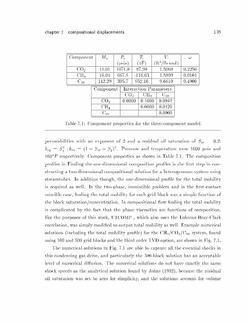
chapter 7 compositional displacements 139
Component Mw Pc Tc Vc !
(psia) (�F) (ft3=lb-mol)CO2 44.01 1071.0 87.90 1.5060 0.2250CH4 16.04 667.8 -116.63 1.5899 0.0104C10 142.29 305.7 652.10 9.6610 0.4900
Component Interaction ParametersCO2 CH4 C10
CO2 0.0000 0.1000 0.0942CH4 | 0.0000 0.0420C10 | | 0.0000
Table 7.1: Component properties for the three-component model.
permeabilities with an exponent of 2 and a residual oil saturation of Sor = 0:2:
krg = S2g; kro = (1 � Sor � Sg)
2. Pressure and temperature were 1600 psia and
160�F respectively. Component properties as shown in Table 7.1. The composition
pro�les in Finding the one-dimensional composition pro�les is the �rst step in con-
structing a two-dimensional compositional solution for a heterogeneous system using
streamtubes. In addition though, the one-dimensional pro�le for the total mobility
is required as well. In the two-phase, immiscible problem and in the �rst-contact
miscible case, �nding the total mobility for each grid block was a simple function of
the block saturation/concentration. In compositional ow �nding the total mobility
is complicated by the fact that the phase viscosities are functions of composition.
For the purposes of this work, UTCOMP , which also uses the Lohrenz-Bray-Clark
correlation, was simply modi�ed to output total mobility as well. Example numerical
solutions (including the total mobility pro�le) for the CH4=CO2=C10 system, found
using 100 and 500 grid blocks and the third order TVD-option, are shown in Fig. 7.1.
The numerical solutions in Fig. 7.1 are able to capture all the essential shocks in
this condensing gas drive, and particularly the 500-block solution has an acceptable
level of numerical di�usion. The numerical solutions do not have exactly the same
shock speeds as the analytical solution found by Johns (1992), because the residual
oil saturation was set to zero for simplicity, and the solutions account for volume
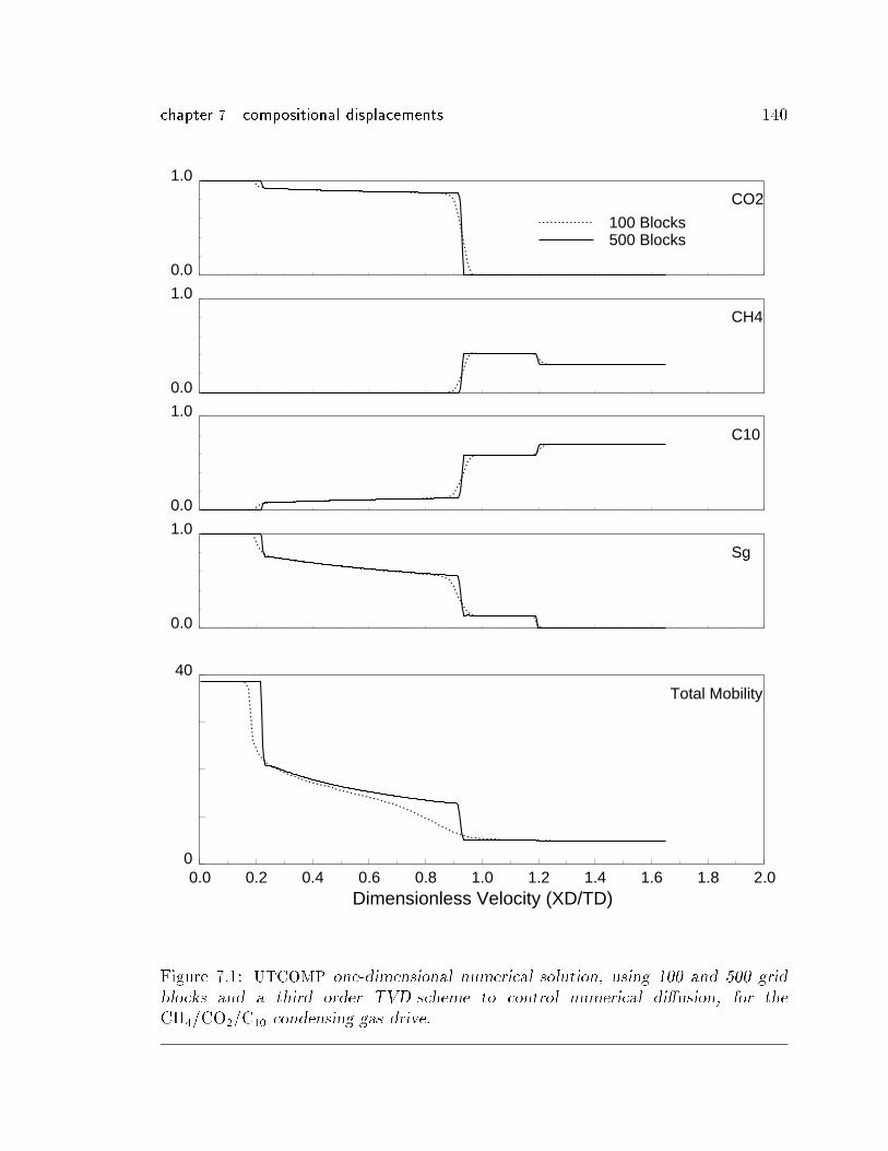
chapter 7 compositional displacements 140
CO2
CH4
C10
Sg
Total Mobility
100 Blocks500 Blocks
0.0
1.0
0.0
1.0
0.0
1.0
0.0
1.0
0
40
0.0 0.2 0.4 0.6 0.8 1.0 1.2 1.4 1.6 1.8 2.0Dimensionless Velocity (XD/TD)
Figure 7.1: UTCOMP one-dimensional numerical solution, using 100 and 500 grid
blocks and a third order TVD-scheme to control numerical di�usion, for the
CH4=CO2=C10 condensing gas drive.
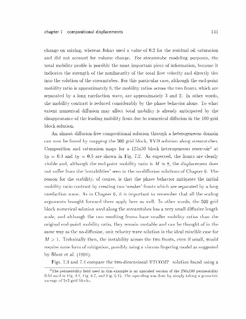
chapter 7 compositional displacements 141
change on mixing, whereas Johns used a value of 0.2 for the residual oil saturation
and did not account for volume change. For streamtube modeling purposes, the
total mobility pro�le is possibly the most important piece of information, because it
indicates the strength of the nonlinearity of the total ow velocity and directly ties
into the solution of the streamtubes. For this particular case, although the end-point
mobility ratio is approximately 8, the mobility ratios across the two fronts, which are
separated by a long rarefaction wave, are approximately 3 and 2. In other words,
the mobility contrast is reduced considerably by the phase behavior alone. To what
extent numerical di�usion may a�ect total mobility is already anticipated by the
disappearance of the leading mobility front due to numerical di�usion in the 100 grid
block solution.
An almost di�usion-free compositional solution through a heterogeneous domain
can now be found by mapping the 500 grid block, TVD solution along streamtubes.
Composition and saturation maps for a 125x50 block heterogeneous reservoir3 at
tD = 0:3 and tD = 0:5 are shown in Fig. 7.2. As expected, the fronts are clearly
visible and, although the end-point mobility ratio is M � 8, the displacement does
not su�er from the `instabilities' seen in the no-di�usion solutions of Chapter 6. The
reason for the stability, of course, is that the phase behavior mitigates the initial
mobility ratio contrast by creating two `weaker' fronts which are separated by a long
rarefaction wave. As in Chapter 6, it is important to remember that all the scaling
arguments brought forward there apply here as well. In other words, the 500 grid
block numerical solution used along the streamtubes has a very small di�usive length
scale, and although the two resulting fronts have smaller mobility ratios than the
original end-point mobility ratio, they remain unstable and can be thought of in the
same way as the no-di�usion, unit velocity wave solution in the ideal miscible case for
M > 1. Technically then, the instability across the two fronts, even if small, would
require some form of mitigation, possibly using a viscous �ngering model as suggested
by Blunt et al. (1994).
Figs. 7.3 and 7.4 compare the two-dimensional UTCOMP solution found using a
3The permeability �eld used in this example is an upscaled version of the 250x100 permeability�eld used in Fig. 4.1, Fig. 6.7, and Fig. 6.15. The upscaling was done by simply taking a geometricaverage of 2x2 grid blocks.
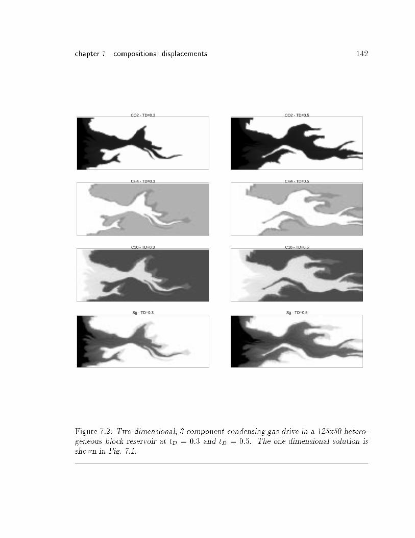
chapter 7 compositional displacements 142
CO2 - TD=0.3
CH4 - TD=0.3
C10 - TD=0.3
Sg - TD=0.3
CO2 - TD=0.5
CH4 - TD=0.5
C10 - TD=0.5
Sg - TD=0.5
Figure 7.2: Two-dimensional, 3 component condensing gas drive in a 125x50 hetero-
geneous block reservoir at tD = 0:3 and tD = 0:5. The one-dimensional solution isshown in Fig. 7.1.
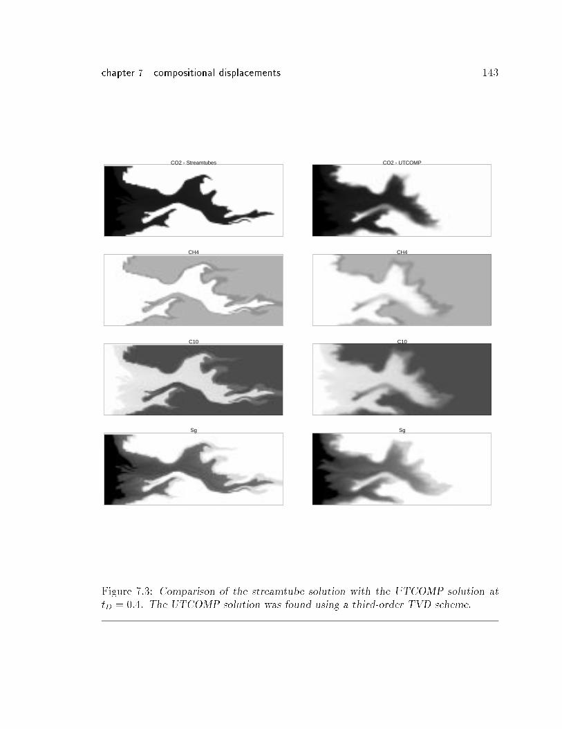
chapter 7 compositional displacements 143
CO2 - Streamtubes
CH4
C10
Sg
CO2 - UTCOMP
CH4
C10
Sg
Figure 7.3: Comparison of the streamtube solution with the UTCOMP solution attD = 0:4. The UTCOMP solution was found using a third-order TVD scheme.
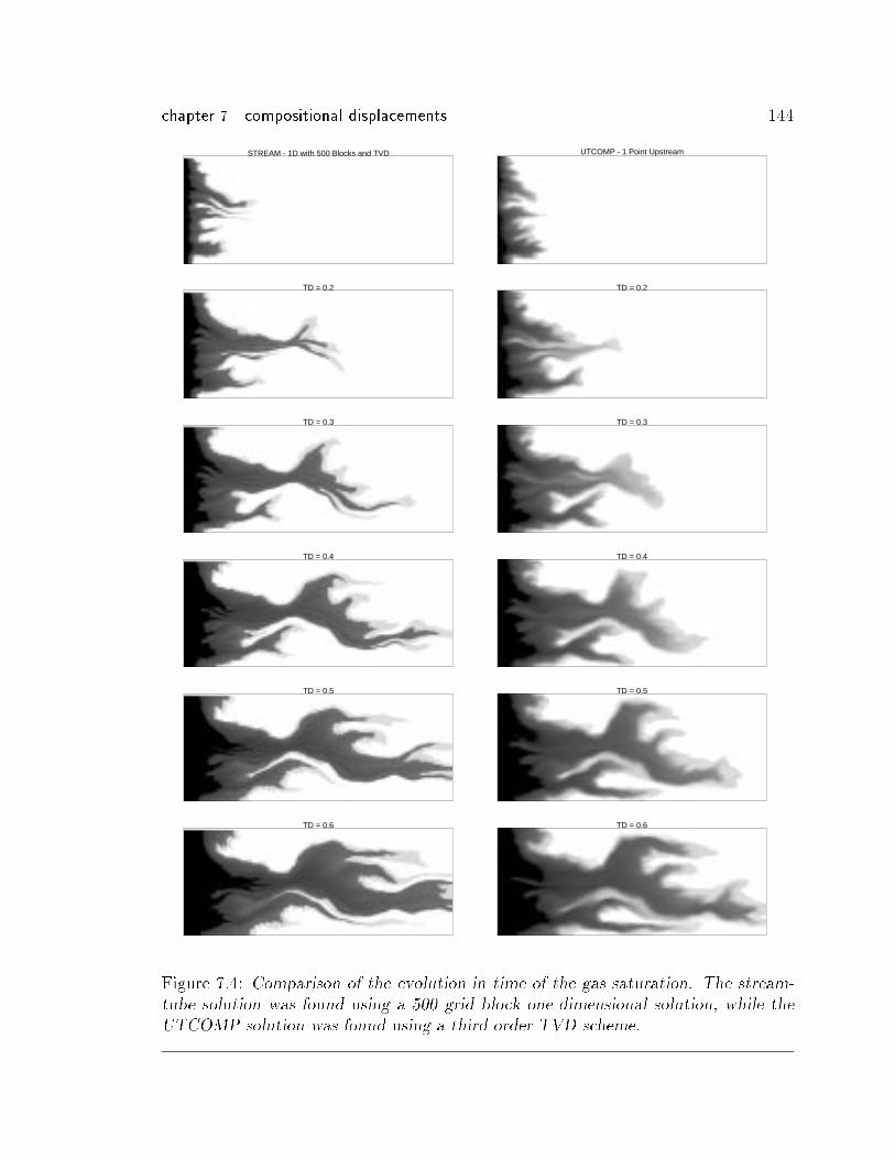
chapter 7 compositional displacements 144
STREAM - 1D with 500 Blocks and TVD
TD = 0.2
TD = 0.3
TD = 0.4
TD = 0.5
TD = 0.6
UTCOMP - 1 Point Upstream
TD = 0.2
TD = 0.3
TD = 0.4
TD = 0.5
TD = 0.6
Figure 7.4: Comparison of the evolution in time of the gas saturation. The stream-
tube solution was found using a 500 grid block one-dimensional solution, while the
UTCOMP solution was found using a third-order TVD scheme.
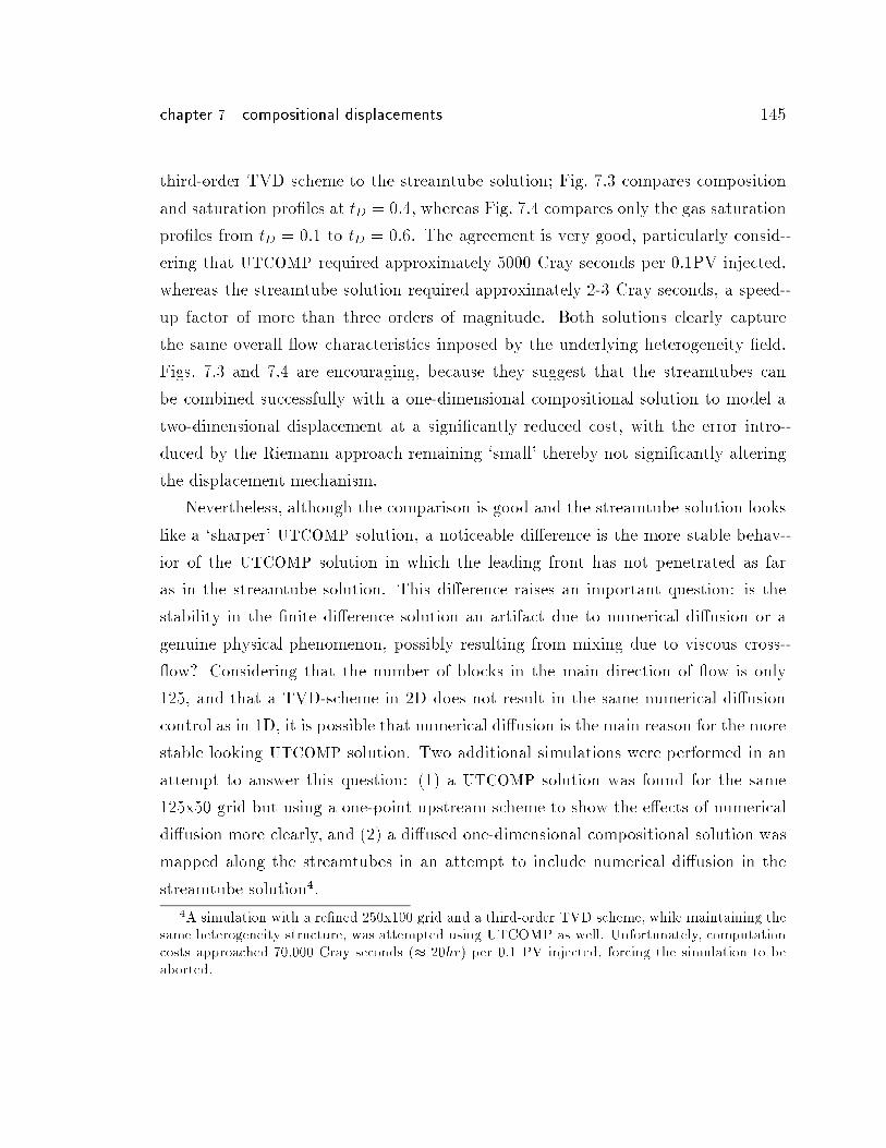
chapter 7 compositional displacements 145
third-order TVD scheme to the streamtube solution; Fig. 7.3 compares composition
and saturation pro�les at tD = 0:4, whereas Fig. 7.4 compares only the gas saturation
pro�les from tD = 0:1 to tD = 0:6. The agreement is very good, particularly consid-
ering that UTCOMP required approximately 5000 Cray seconds per 0.1PV injected,
whereas the streamtube solution required approximately 2-3 Cray seconds, a speed-
up factor of more than three orders of magnitude. Both solutions clearly capture
the same overall ow characteristics imposed by the underlying heterogeneity �eld.
Figs. 7.3 and 7.4 are encouraging, because they suggest that the streamtubes can
be combined successfully with a one-dimensional compositional solution to model a
two-dimensional displacement at a signi�cantly reduced cost, with the error intro-
duced by the Riemann approach remaining `small' thereby not signi�cantly altering
the displacement mechanism.
Nevertheless, although the comparison is good and the streamtube solution looks
like a `sharper' UTCOMP solution, a noticeable di�erence is the more stable behav-
ior of the UTCOMP solution in which the leading front has not penetrated as far
as in the streamtube solution. This di�erence raises an important question: is the
stability in the �nite di�erence solution an artifact due to numerical di�usion or a
genuine physical phenomenon, possibly resulting from mixing due to viscous cross-
ow? Considering that the number of blocks in the main direction of ow is only
125, and that a TVD-scheme in 2D does not result in the same numerical di�usion
control as in 1D, it is possible that numerical di�usion is the main reason for the more
stable looking UTCOMP solution. Two additional simulations were performed in an
attempt to answer this question: (1) a UTCOMP solution was found for the same
125x50 grid but using a one-point upstream scheme to show the e�ects of numerical
di�usion more clearly, and (2) a di�used one-dimensional compositional solution was
mapped along the streamtubes in an attempt to include numerical di�usion in the
streamtube solution4.
4A simulation with a re�ned 250x100 grid and a third-order TVD scheme, while maintaining thesame heterogeneity structure, was attempted using UTCOMP as well. Unfortunately, computationcosts approached 70,000 Cray seconds (� 20hr) per 0.1 PV injected, forcing the simulation to beaborted.
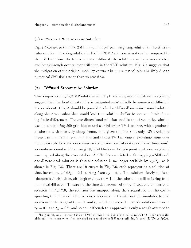
chapter 7 compositional displacements 146
(1) - 125x50 1Pt Upstream Solution
Fig. 7.5 compares the UTCOMP one-point upstream weighting solution to the stream-
tube solution. The degradation in the UTCOMP solution is noticeable compared to
the TVD solution: the fronts are more di�used, the solution now looks more stable,
and breakthrough occurs later still than in the TVD solution. Fig. 7.5 suggests that
the mitigation of the original mobility contrast in UTCOMP solutions is likely due to
numerical di�usion rather than to cross ow.
(2) - Di�used Streamtube Solution
The comparison of UTCOMP solutions with TVD and single-point upstream weighting
suggest that the frontal instability is mitigated substantially by numerical di�usion.
To corroborate this, it should be possible to �nd a `di�used' one-dimensional solution
along the streamtubes that would lead to a solution similar to the one obtained us-
ing �nite di�erences. The one-dimensional solution used in the streamtube solution
was obtained using 500 grid blocks and a third-order TVD scheme, which produced
a solution with relatively sharp fronts. But given the fact that only 125 blocks are
present in the main direction of ow and that a TVD scheme in two-dimensions does
not necessarily have the same numerical di�usion control as it does in one dimension5,
a one-dimensional solution using 100 grid blocks and single point upstream weighting
was mapped along the streamtubes. A di�culty associated with mapping a `di�used'
one-dimensional solution is that the solution is no longer scalable by xD=tD, as is
shown in Fig. 7.6. There are 10 curves in Fig. 7.6, each representing a solution at
time increments of �tD = 0:1 starting from tD = 0:1. The solution clearly tends to
`sharpen-up' with time, although even at tD = 1:0, the solution is still su�ering from
numerical di�usion. To capture the time dependence of the di�used, one-dimensional
solution in Fig. 7.6, the solution was mapped along the streamtube for the corre-
sponding time interval: the �rst curve was used in the streamtube simulator to �nd
solutions in the range of tD = 0:0 and tD = 0:1, the second curve for solutions between
tD = 0:1 and tD = 0:2, and so on. Although this approach is only a rough attempt to
5In general, any method that is TVD in two dimensions will be at most �rst order accurate,although the accuracy can be increased to second order if Strang splitting is used (LeVeque 1992).
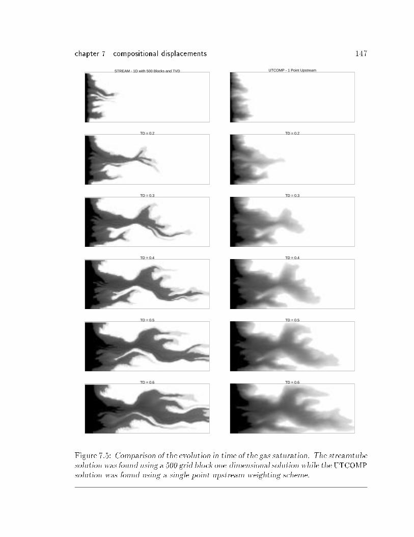
chapter 7 compositional displacements 147
STREAM - 1D with 500 Blocks and TVD
TD = 0.2
TD = 0.3
TD = 0.4
TD = 0.5
TD = 0.6
UTCOMP - 1 Point Upstream
TD = 0.2
TD = 0.3
TD = 0.4
TD = 0.5
TD = 0.6
Figure 7.5: Comparison of the evolution in time of the gas saturation. The streamtubesolution was found using a 500 grid block one-dimensional solution while the UTCOMP
solution was found using a single-point upstream weighting scheme.
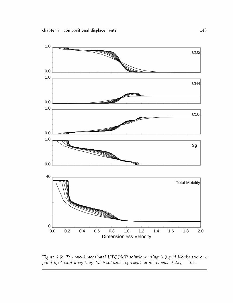
chapter 7 compositional displacements 148
CO2
CH4
C10
Sg
Total Mobility
0.0
1.0
0.0
1.0
0.0
1.0
0.0
1.0
0
40
0.0 0.2 0.4 0.6 0.8 1.0 1.2 1.4 1.6 1.8 2.0Dimensionless Velocity
Figure 7.6: Ten one-dimensional UTCOMP solutions using 100 grid blocks and one
point upstream weighting. Each solution represent an increment of �tD = 0:1.
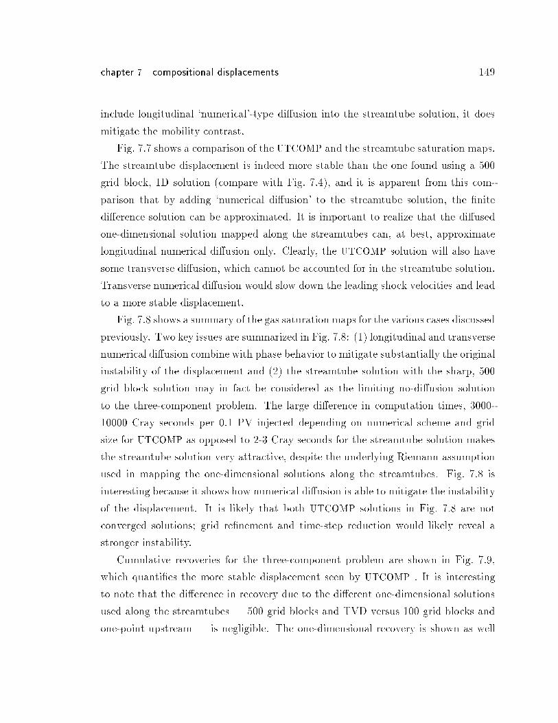
chapter 7 compositional displacements 149
include longitudinal `numerical'-type di�usion into the streamtube solution, it does
mitigate the mobility contrast.
Fig. 7.7 shows a comparison of the UTCOMP and the streamtube saturation maps.
The streamtube displacement is indeed more stable than the one found using a 500
grid block, 1D solution (compare with Fig. 7.4), and it is apparent from this com-
parison that by adding `numerical di�usion' to the streamtube solution, the �nite
di�erence solution can be approximated. It is important to realize that the di�used
one-dimensional solution mapped along the streamtubes can, at best, approximate
longitudinal numerical di�usion only. Clearly, the UTCOMP solution will also have
some transverse di�usion, which cannot be accounted for in the streamtube solution.
Transverse numerical di�usion would slow down the leading shock velocities and lead
to a more stable displacement.
Fig. 7.8 shows a summary of the gas saturation maps for the various cases discussed
previously. Two key issues are summarized in Fig. 7.8: (1) longitudinal and transverse
numerical di�usion combine with phase behavior to mitigate substantially the original
instability of the displacement and (2) the streamtube solution with the sharp, 500
grid block solution may in fact be considered as the limiting no-di�usion solution
to the three-component problem. The large di�erence in computation times, 3000-
10000 Cray seconds per 0.1 PV injected depending on numerical scheme and grid
size for UTCOMP as opposed to 2-3 Cray seconds for the streamtube solution makes
the streamtube solution very attractive, despite the underlying Riemann assumption
used in mapping the one-dimensional solutions along the streamtubes. Fig. 7.8 is
interesting because it shows how numerical di�usion is able to mitigate the instability
of the displacement. It is likely that both UTCOMP solutions in Fig. 7.8 are not
converged solutions; grid re�nement and time-step reduction would likely reveal a
stronger instability.
Cumulative recoveries for the three-component problem are shown in Fig. 7.9,
which quanti�es the more stable displacement seen by UTCOMP . It is interesting
to note that the di�erence in recovery due to the di�erent one-dimensional solutions
used along the streamtubes | 500 grid blocks and TVD versus 100 grid blocks and
one-point upstream | is negligible. The one-dimensional recovery is shown as well
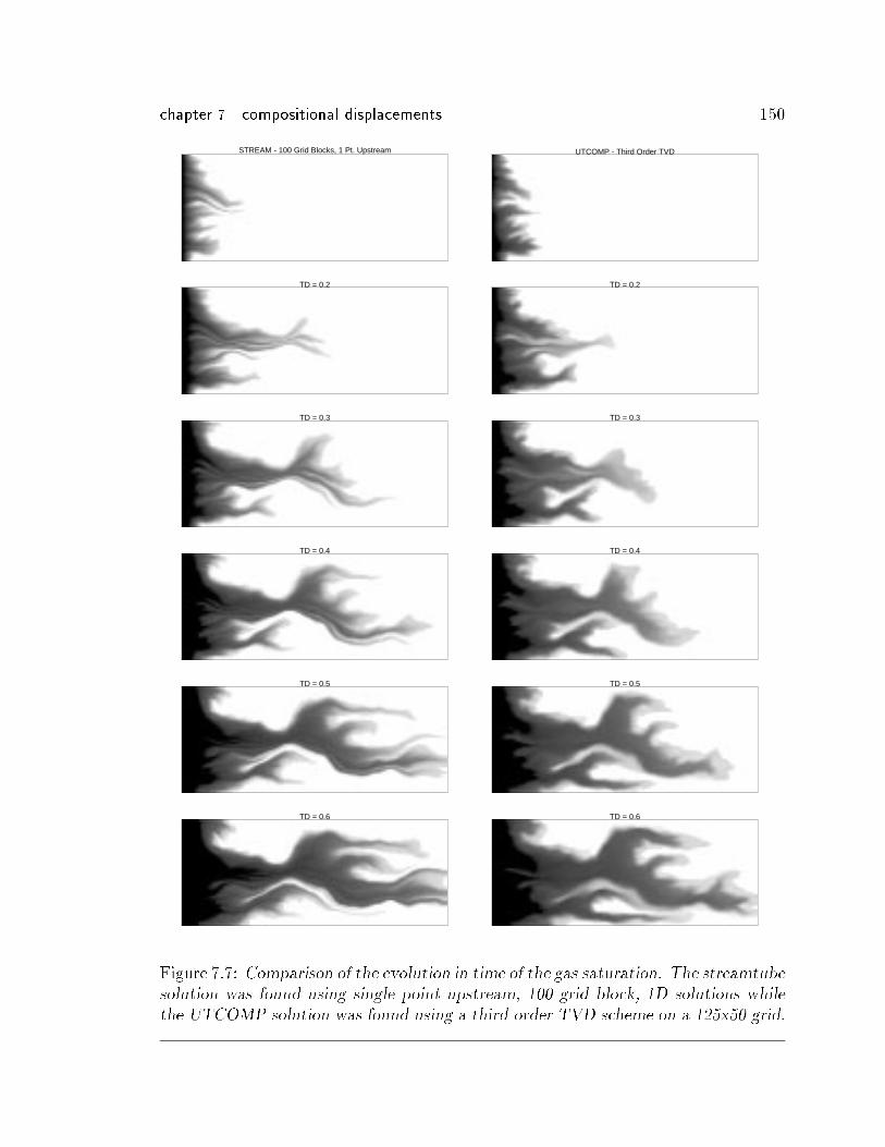
chapter 7 compositional displacements 150
STREAM - 100 Grid Blocks, 1 Pt. Upstream
TD = 0.2
TD = 0.3
TD = 0.4
TD = 0.5
TD = 0.6
UTCOMP - Third Order TVD
TD = 0.2
TD = 0.3
TD = 0.4
TD = 0.5
TD = 0.6
Figure 7.7: Comparison of the evolution in time of the gas saturation. The streamtubesolution was found using single point upstream, 100 grid block, 1D solutions while
the UTCOMP solution was found using a third-order TVD scheme on a 125x50 grid.
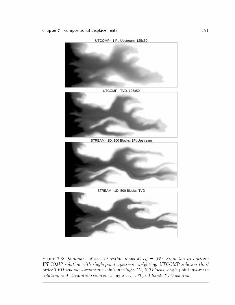
chapter 7 compositional displacements 151
UTCOMP - 1 Pt. Upstream, 125x50
UTCOMP - TVD, 125x50
STREAM - 1D, 100 Blocks, 1Pt Upstream
STREAM - 1D, 500 Blocks, TVD
Figure 7.8: Summary of gas saturation maps at tD = 0:5: From top to bottom:
UTCOMP solution with single-point upstream weighting, UTCOMP solution third
order TVD scheme, streamtube solution using a 1D, 100 blocks, single-point upstream
solution, and streamtube solution using a 1D, 500 grid block-TVD solution.
chapter 7 compositional displacements 152
0.0
0.2
0.4
0.6
0.8
1.0
Fra
ctio
n of
Initi
al O
il in
Pla
ce, N
pD
0.0 0.2 0.4 0.6 0.8 1.0 1.2 1.4 1.6 1.8 2.0Dimensionless Time, tD
aa
a
a
aaaaaaaaaaaaa
a
a
a
a
a
a
a
a
a
a
a
aaa
a
a
aa
aa
a a
a
1DStream - 1Pt (100 Blocks)Stream - TVD (500 Blocks)UTCOMP
Figure 7.9: Recovery curves for the CO2=CH4=C10 system.
as a way to quantify the impact on recovery due to heterogeneity and a nonlinear
velocity �eld. Fig. 7.10 shows the convergence of the streamtube solution. Forty
streamtubes updates are su�cient to capture the �rst order e�ect imposed by reservoir
heterogeneity on recovery, and, as expected, the UTCOMP recovery falls between the
streamtube solutions using a single solve and ten solves.
Fig. 7.11 shows the same three-component, two-phase displacement through a
less heterogeneous system. The permeability �eld is an upscaled version (125x50) of
the same permeability �eld used for the displacements shown in Fig. 6.20 (� = 1:00,
�ln k = 0:5,HI = 0:25). The interesting feature of Fig. 7.11 is that while the UTCOMP
single-point upstream solution shows no viscous �ngering whatsoever, the same solu-
tion using a third-order TVD scheme is able to retain su�cient mobility contrast to
result in some �ngering in the channel demonstrating again that numerical di�usion
can have a substantial impact on ow behavior and supress �ngering. The streamtube
solution, of course, is not able to reproduce any viscous �ngering, but captures the
main ow path and the �rst order e�ect of heterogeneity on the displacement at a
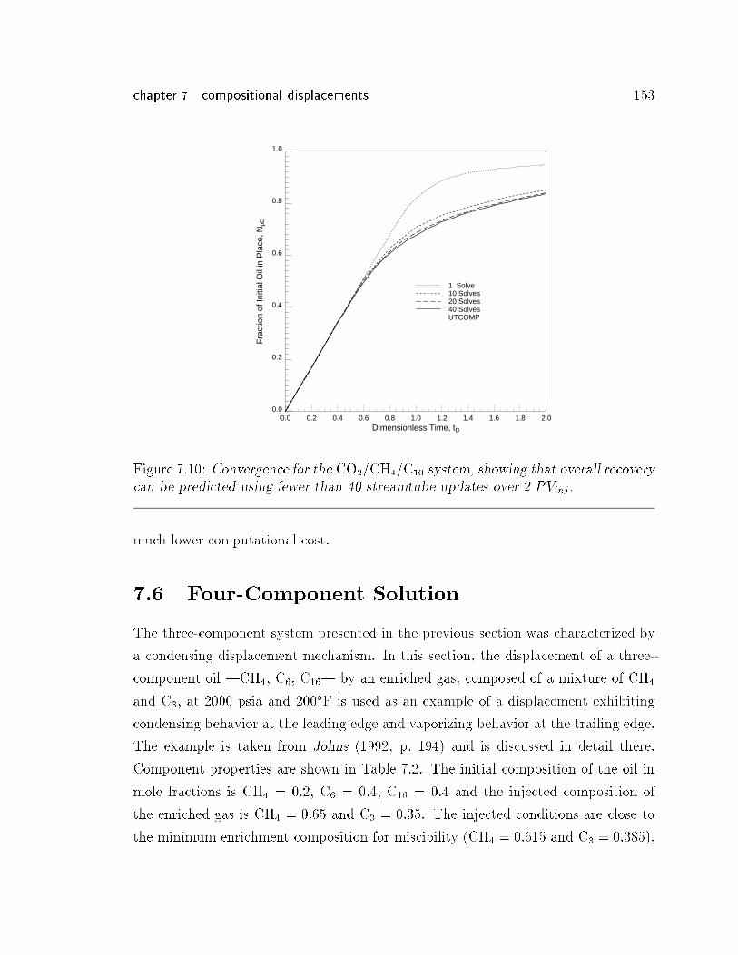
chapter 7 compositional displacements 153
0.0
0.2
0.4
0.6
0.8
1.0
Fra
ctio
n of
Initi
al O
il in
Pla
ce, N
pD
0.0 0.2 0.4 0.6 0.8 1.0 1.2 1.4 1.6 1.8 2.0Dimensionless Time, tD
1 Solve10 Solves20 Solves40 SolvesUTCOMP
Figure 7.10: Convergence for the CO2=CH4=C10 system, showing that overall recoverycan be predicted using fewer than 40 streamtube updates over 2 PVinj .
much lower computational cost.
7.6 Four-Component Solution
The three-component system presented in the previous section was characterized by
a condensing displacement mechanism. In this section, the displacement of a three-
component oil |CH4, C6, C16| by an enriched gas, composed of a mixture of CH4
and C3, at 2000 psia and 200�F is used as an example of a displacement exhibiting
condensing behavior at the leading edge and vaporizing behavior at the trailing edge.
The example is taken from Johns (1992, p. 194) and is discussed in detail there.
Component properties are shown in Table 7.2. The initial composition of the oil in
mole fractions is CH4 = 0:2, C6 = 0:4, C16 = 0:4 and the injected composition of
the enriched gas is CH4 = 0:65 and C3 = 0:35. The injected conditions are close to
the minimum enrichment composition for miscibility (CH4 = 0:615 and C3 = 0:385),
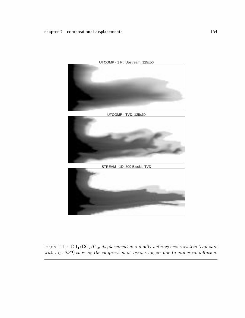
chapter 7 compositional displacements 154
UTCOMP - 1 Pt. Upstream, 125x50
UTCOMP - TVD, 125x50
STREAM - 1D, 500 Blocks, TVD
Figure 7.11: CH4=CO2=C10 displacement in a mildly heterogeneous system (compare
with Fig. 6.20) showing the suppression of viscous �ngers due to numerical di�usion.
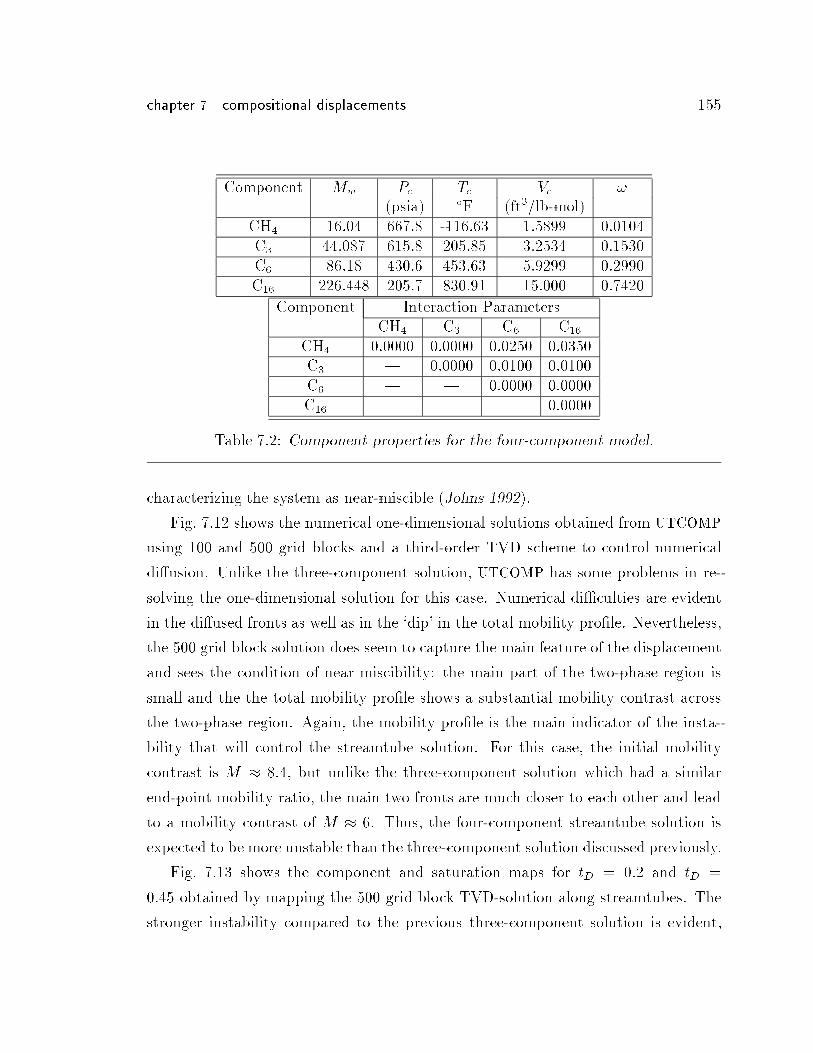
chapter 7 compositional displacements 155
Component Mw Pc Tc Vc !
(psia) �F (ft3=lb-mol)CH4 16.04 667.8 -116.63 1.5899 0.0104C3 44.087 615.8 205.85 3.2534 0.1530C6 86.18 430.6 453.63 5.9299 0.2990C16 226.448 205.7 830.91 15.000 0.7420
Component Interaction ParametersCH4 C3 C6 C16
CH4 0.0000 0.0000 0.0250 0.0350C3 | 0.0000 0.0100 0.0100C6 | | 0.0000 0.0000C16 | | | 0.0000
Table 7.2: Component properties for the four-component model.
characterizing the system as near-miscible (Johns 1992).
Fig. 7.12 shows the numerical one-dimensional solutions obtained from UTCOMP
using 100 and 500 grid blocks and a third-order TVD scheme to control numerical
di�usion. Unlike the three-component solution, UTCOMP has some problems in re-
solving the one-dimensional solution for this case. Numerical di�culties are evident
in the di�used fronts as well as in the `dip' in the total mobility pro�le. Nevertheless,
the 500 grid block solution does seem to capture the main feature of the displacement
and sees the condition of near miscibility: the main part of the two-phase region is
small and the the total mobility pro�le shows a substantial mobility contrast across
the two-phase region. Again, the mobility pro�le is the main indicator of the insta-
bility that will control the streamtube solution. For this case, the initial mobility
contrast is M � 8:4, but unlike the three-component solution which had a similar
end-point mobility ratio, the main two fronts are much closer to each other and lead
to a mobility contrast of M � 6. Thus, the four-component streamtube solution is
expected to be more unstable than the three-component solution discussed previously.
Fig. 7.13 shows the component and saturation maps for tD = 0:2 and tD =
0:45 obtained by mapping the 500 grid block TVD-solution along streamtubes. The
stronger instability compared to the previous three-component solution is evident,
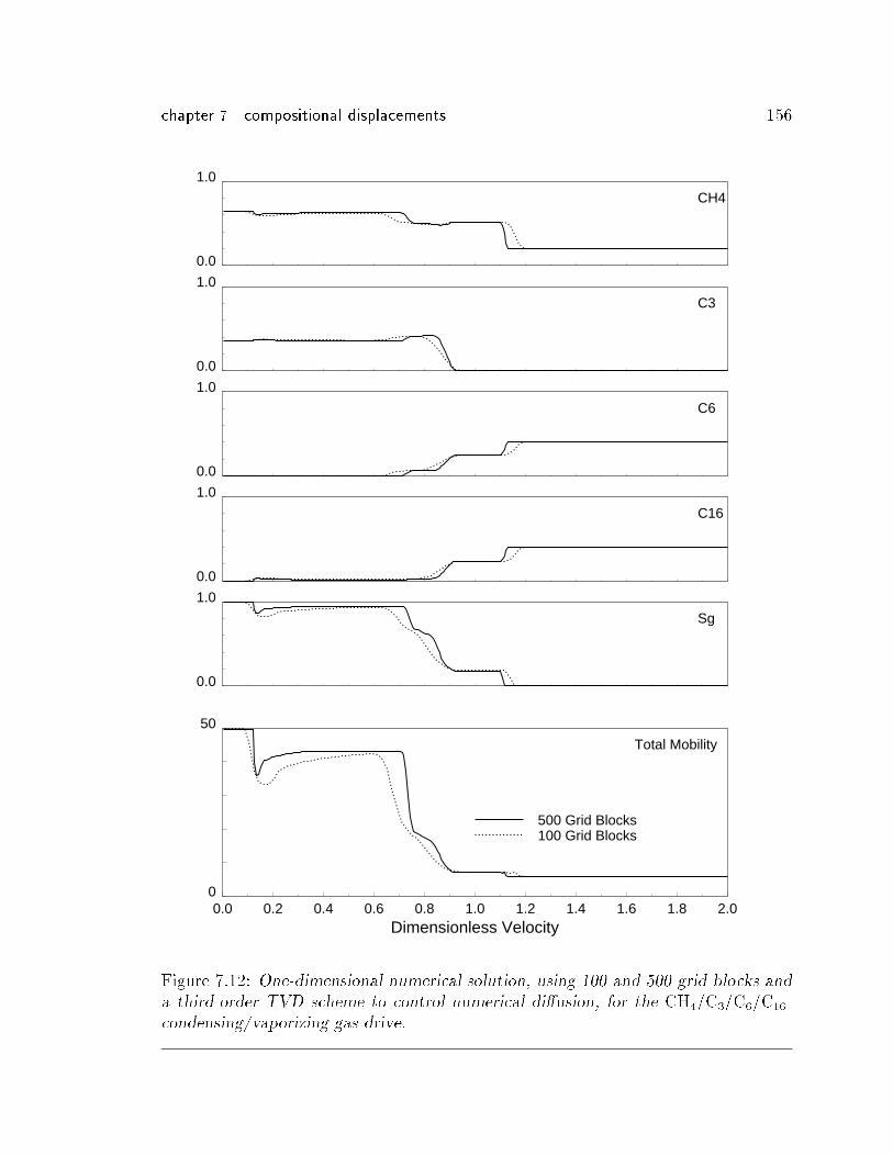
chapter 7 compositional displacements 156
0.0
1.0
0.0
1.0
0.0
1.0
0.0
1.0
0.0
1.0
0
50
0.0 0.2 0.4 0.6 0.8 1.0 1.2 1.4 1.6 1.8 2.0Dimensionless Velocity
500 Grid Blocks100 Grid Blocks
CH4
C3
C6
C16
Sg
Total Mobility
Figure 7.12: One-dimensional numerical solution, using 100 and 500 grid blocks and
a third-order TVD scheme to control numerical di�usion, for the CH4=C3=C6=C16-
condensing/vaporizing gas drive.
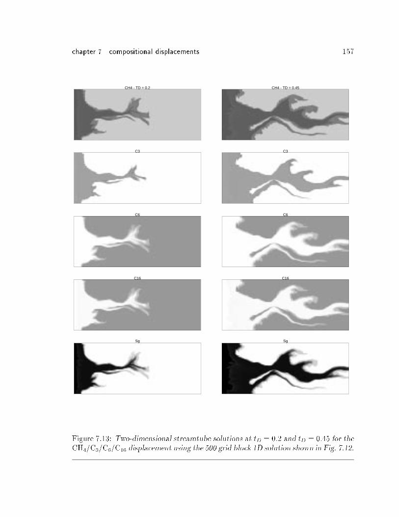
chapter 7 compositional displacements 157
CH4 - TD = 0.2
C3
C6
C16
Sg
CH4 - TD = 0.45
C3
C6
C16
Sg
Figure 7.13: Two-dimensional streamtube solutions at tD = 0:2 and tD = 0:45 for theCH4=C3=C6=C16 displacement using the 500 grid block 1D solution shown in Fig. 7.12.
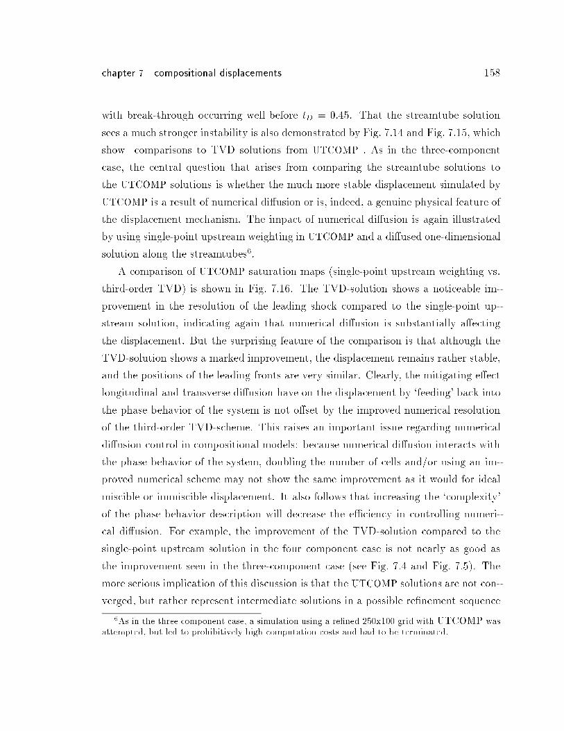
chapter 7 compositional displacements 158
with break-through occurring well before tD = 0:45. That the streamtube solution
sees a much stronger instability is also demonstrated by Fig. 7.14 and Fig. 7.15, which
show comparisons to TVD solutions from UTCOMP . As in the three-component
case, the central question that arises from comparing the streamtube solutions to
the UTCOMP solutions is whether the much more stable displacement simulated by
UTCOMP is a result of numerical di�usion or is, indeed, a genuine physical feature of
the displacement mechanism. The impact of numerical di�usion is again illustrated
by using single-point upstream weighting in UTCOMP and a di�used one-dimensional
solution along the streamtubes6.
A comparison of UTCOMP saturation maps (single-point upstream weighting vs.
third-order TVD) is shown in Fig. 7.16. The TVD-solution shows a noticeable im-
provement in the resolution of the leading shock compared to the single-point up-
stream solution, indicating again that numerical di�usion is substantially a�ecting
the displacement. But the surprising feature of the comparison is that although the
TVD-solution shows a marked improvement, the displacement remains rather stable,
and the positions of the leading fronts are very similar. Clearly, the mitigating e�ect
longitudinal and transverse di�usion have on the displacement by `feeding' back into
the phase behavior of the system is not o�set by the improved numerical resolution
of the third-order TVD-scheme. This raises an important issue regarding numerical
di�usion control in compositional models: because numerical di�usion interacts with
the phase behavior of the system, doubling the number of cells and/or using an im-
proved numerical scheme may not show the same improvement as it would for ideal
miscible or immiscible displacement. It also follows that increasing the `complexity'
of the phase behavior description will decrease the e�ciency in controlling numeri-
cal di�usion. For example, the improvement of the TVD-solution compared to the
single-point upstream solution in the four component case is not nearly as good as
the improvement seen in the three-component case (see Fig. 7.4 and Fig. 7.5). The
more serious implication of this discussion is that the UTCOMP solutions are not con-
verged, but rather represent intermediate solutions in a possible re�nement sequence
6As in the three component case, a simulation using a re�ned 250x100 grid with UTCOMP wasattempted, but led to prohibitively high computation costs and had to be terminated.
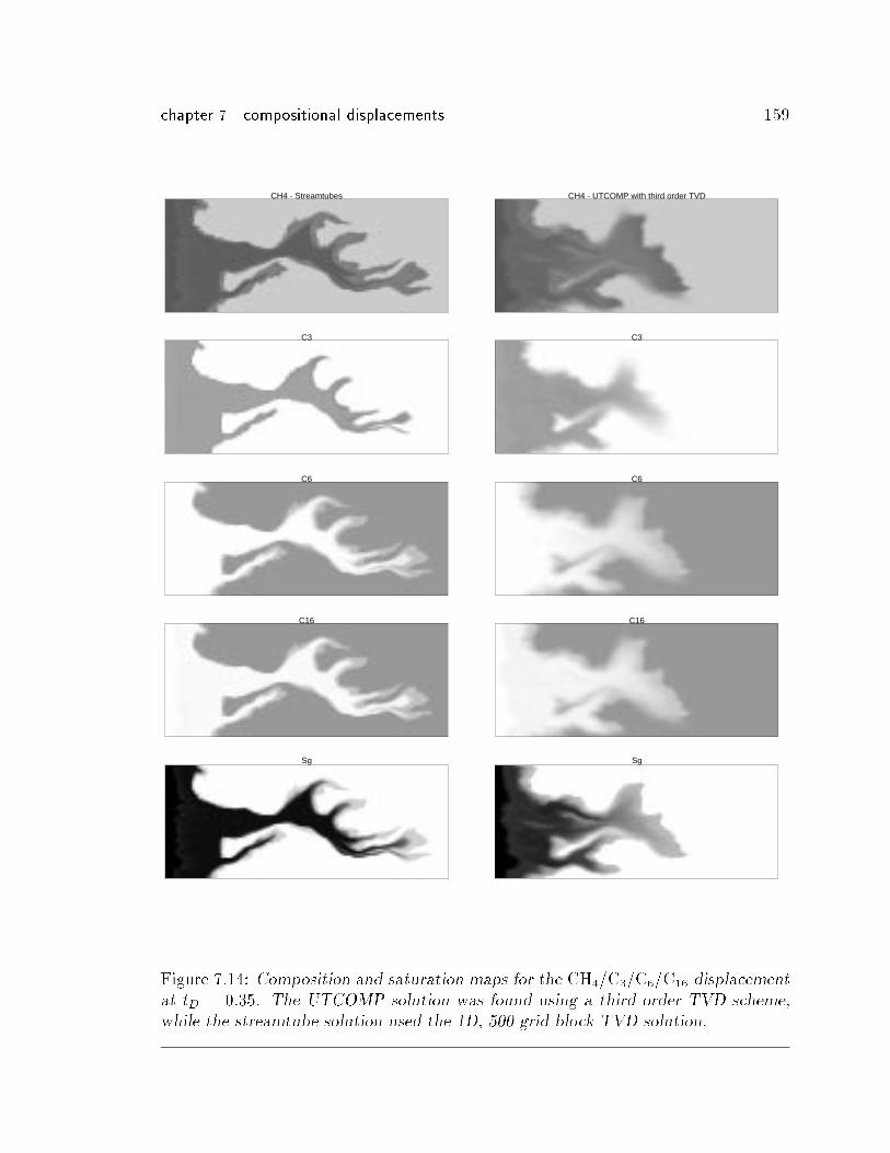
chapter 7 compositional displacements 159
CH4 - Streamtubes
C3
C6
C16
Sg
CH4 - UTCOMP with third order TVD
C3
C6
C16
Sg
Figure 7.14: Composition and saturation maps for the CH4=C3=C6=C16 displacementat tD = 0:35. The UTCOMP solution was found using a third order TVD scheme,
while the streamtube solution used the 1D, 500 grid block TVD solution.
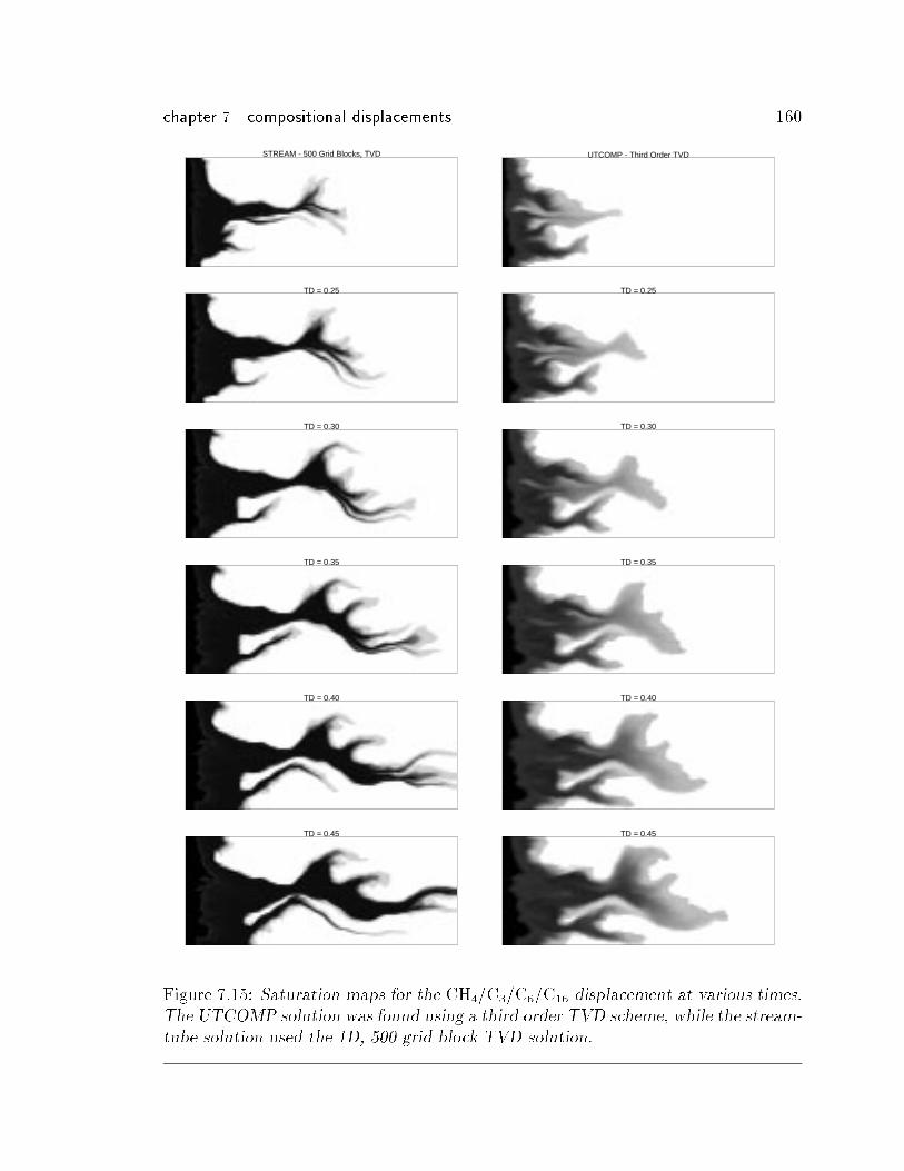
chapter 7 compositional displacements 160
STREAM - 500 Grid Blocks, TVD
TD = 0.25
TD = 0.30
TD = 0.35
TD = 0.40
TD = 0.45
UTCOMP - Third Order TVD
TD = 0.25
TD = 0.30
TD = 0.35
TD = 0.40
TD = 0.45
Figure 7.15: Saturation maps for the CH4=C3=C6=C16 displacement at various times.The UTCOMP solution was found using a third order TVD scheme, while the stream-
tube solution used the 1D, 500 grid block TVD solution.
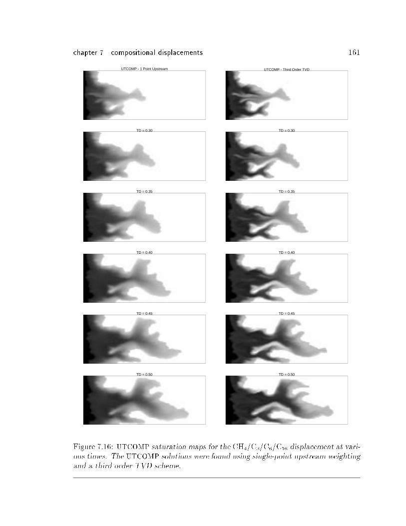
chapter 7 compositional displacements 161
UTCOMP - 1 Point Upstream
TD = 0.30
TD = 0.35
TD = 0.40
TD = 0.45
TD = 0.50
UTCOMP - Third Order TVD
TD = 0.30
TD = 0.35
TD = 0.40
TD = 0.45
TD = 0.50
Figure 7.16: UTCOMP saturation maps for the CH4=C3=C6=C16 displacement at vari-ous times. The UTCOMP solutions were found using single-point upstream weighting
and a third order TVD scheme.
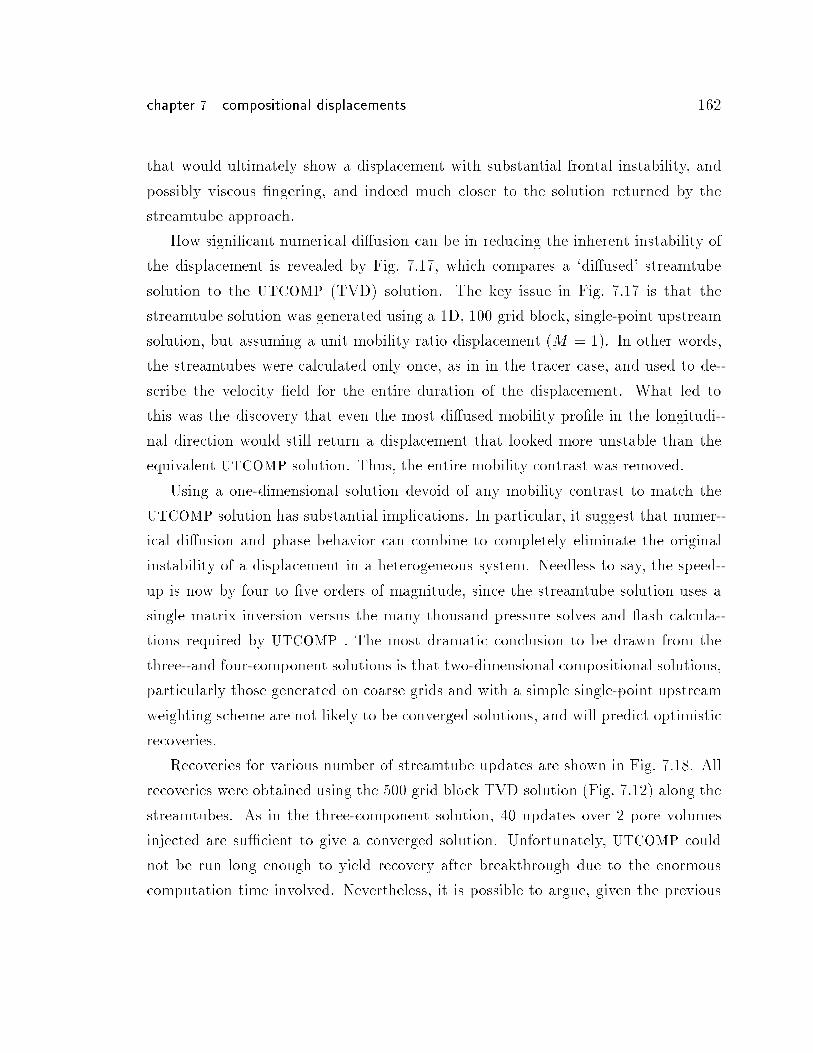
chapter 7 compositional displacements 162
that would ultimately show a displacement with substantial frontal instability, and
possibly viscous �ngering, and indeed much closer to the solution returned by the
streamtube approach.
How signi�cant numerical di�usion can be in reducing the inherent instability of
the displacement is revealed by Fig. 7.17, which compares a `di�used' streamtube
solution to the UTCOMP (TVD) solution. The key issue in Fig. 7.17 is that the
streamtube solution was generated using a 1D, 100 grid block, single-point upstream
solution, but assuming a unit mobility ratio displacement (M = 1). In other words,
the streamtubes were calculated only once, as in in the tracer case, and used to de-
scribe the velocity �eld for the entire duration of the displacement. What led to
this was the discovery that even the most di�used mobility pro�le in the longitudi-
nal direction would still return a displacement that looked more unstable than the
equivalent UTCOMP solution. Thus, the entire mobility contrast was removed.
Using a one-dimensional solution devoid of any mobility contrast to match the
UTCOMP solution has substantial implications. In particular, it suggest that numer-
ical di�usion and phase behavior can combine to completely eliminate the original
instability of a displacement in a heterogeneous system. Needless to say, the speed-
up is now by four to �ve orders of magnitude, since the streamtube solution uses a
single matrix inversion versus the many thousand pressure solves and ash calcula-
tions required by UTCOMP . The most dramatic conclusion to be drawn from the
three- and four-component solutions is that two-dimensional compositional solutions,
particularly those generated on coarse grids and with a simple single-point upstream
weighting scheme are not likely to be converged solutions, and will predict optimistic
recoveries.
Recoveries for various number of streamtube updates are shown in Fig. 7.18. All
recoveries were obtained using the 500 grid block TVD solution (Fig. 7.12) along the
streamtubes. As in the three-component solution, 40 updates over 2 pore volumes
injected are su�cient to give a converged solution. Unfortunately, UTCOMP could
not be run long enough to yield recovery after breakthrough due to the enormous
computation time involved. Nevertheless, it is possible to argue, given the previous
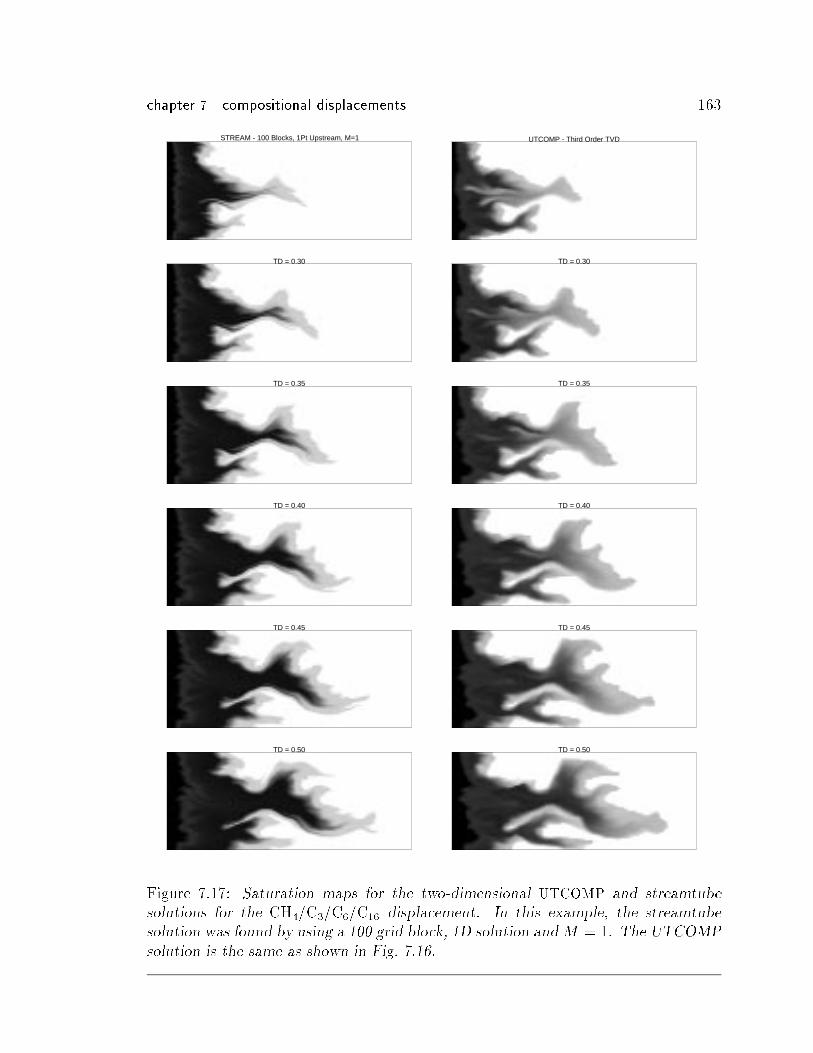
chapter 7 compositional displacements 163
STREAM - 100 Blocks, 1Pt Upstream, M=1
TD = 0.30
TD = 0.35
TD = 0.40
TD = 0.45
TD = 0.50
UTCOMP - Third Order TVD
TD = 0.30
TD = 0.35
TD = 0.40
TD = 0.45
TD = 0.50
Figure 7.17: Saturation maps for the two-dimensional UTCOMP and streamtube
solutions for the CH4=C3=C6=C16 displacement. In this example, the streamtube
solution was found by using a 100 grid block, 1D solution andM = 1. The UTCOMP
solution is the same as shown in Fig. 7.16.
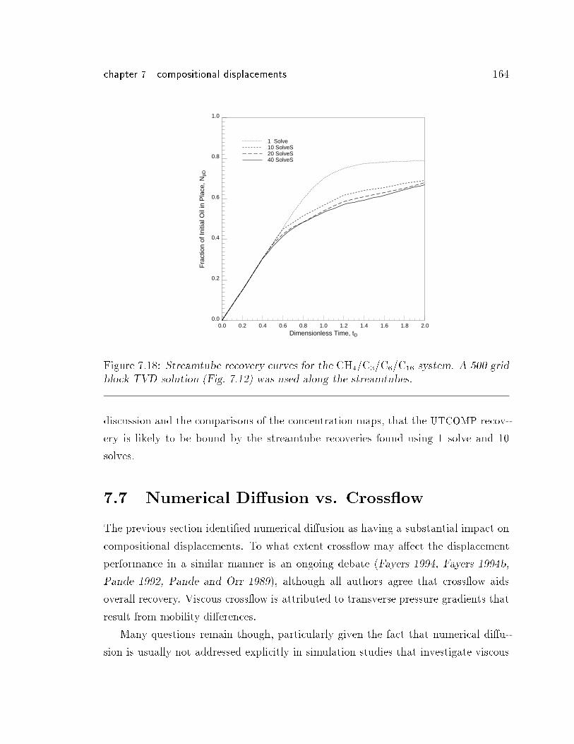
chapter 7 compositional displacements 164
0.0
0.2
0.4
0.6
0.8
1.0
Fra
ctio
n of
Initi
al O
il in
Pla
ce, N
pD
0.0 0.2 0.4 0.6 0.8 1.0 1.2 1.4 1.6 1.8 2.0Dimensionless Time, tD
1 Solve10 SolveS20 SolveS40 SolveS
Figure 7.18: Streamtube recovery curves for the CH4=C3=C6=C16 system. A 500 gridblock TVD solution (Fig. 7.12) was used along the streamtubes.
discussion and the comparisons of the concentration maps, that the UTCOMP recov-
ery is likely to be bound by the streamtube recoveries found using 1 solve and 10
solves.
7.7 Numerical Di�usion vs. Cross ow
The previous section identi�ed numerical di�usion as having a substantial impact on
compositional displacements. To what extent cross ow may a�ect the displacement
performance in a similar manner is an ongoing debate (Fayers 1994, Fayers 1994b,
Pande 1992, Pande and Orr 1989), although all authors agree that cross ow aids
overall recovery. Viscous cross ow is attributed to transverse pressure gradients that
result from mobility di�erences.
Many questions remain though, particularly given the fact that numerical di�u-
sion is usually not addressed explicitly in simulation studies that investigate viscous
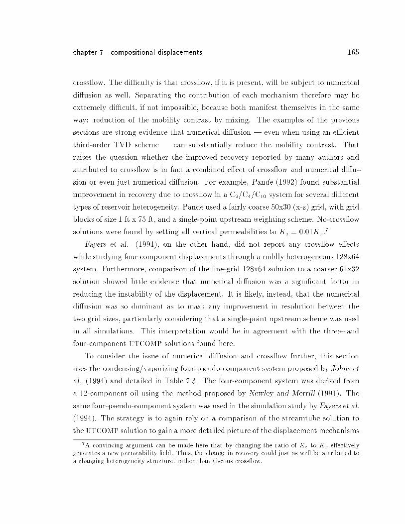
chapter 7 compositional displacements 165
cross ow. The di�culty is that cross ow, if it is present, will be subject to numerical
di�usion as well. Separating the contribution of each mechanism therefore may be
extremely di�cult, if not impossible, because both manifest themselves in the same
way: reduction of the mobility contrast by mixing. The examples of the previous
sections are strong evidence that numerical di�usion | even when using an e�cient
third-order TVD scheme | can substantially reduce the mobility contrast. That
raises the question whether the improved recovery reported by many authors and
attributed to cross ow is in fact a combined e�ect of cross ow and numerical di�u-
sion or even just numerical di�usion. For example, Pande (1992) found substantial
improvement in recovery due to cross ow in a C2=C4=C10 system for several di�erent
types of reservoir heterogeneity. Pande used a fairly coarse 50x30 (x-z) grid, with grid
blocks of size 1 ft x 75 ft, and a single-point upstream weighting scheme. No-cross ow
solutions were found by setting all vertical permeabilities to Kz = 0:01Kx.7
Fayers et al. (1994), on the other hand, did not report any cross ow e�ects
while studying four component displacements through a mildly heterogeneous 128x64
system. Furthermore, comparison of the �ne-grid 128x64 solution to a coarser 64x32
solution showed little evidence that numerical di�usion was a signi�cant factor in
reducing the instability of the displacement. It is likely, instead, that the numerical
di�usion was so dominant as to mask any improvement in resolution between the
two grid sizes, particularly considering that a single-point upstream scheme was used
in all simulations. This interpretation would be in agreement with the three- and
four-component UTCOMP solutions found here.
To consider the issue of numerical di�usion and cross ow further, this section
uses the condensing/vaporizing four-pseudo-component system proposed by Johns et
al. (1994) and detailed in Table 7.3. The four-component system was derived from
a 12-component oil using the method proposed by Newley and Merrill (1991). The
same four-pseudo-component system was used in the simulation study by Fayers et al.
(1994). The strategy is to again rely on a comparison of the streamtube solution to
the UTCOMP solution to gain a more detailed picture of the displacement mechanisms
7A convincing argument can be made here that by changing the ratio of Kz to Kx e�ectivelygenerates a new permeability �eld. Thus, the change in recovery could just as well be attributed toa changing heterogeneity structure, rather than viscous cross ow.
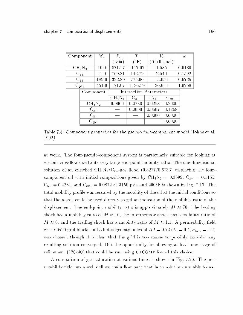
chapter 7 compositional displacements 166
Component Mw Pc Tc Vc !
(psia) (�F) (ft3=lb-mol)CH4N2 16.0 671.17 -117.07 1.585 0.0130C2+ 41.0 769.81 142.79 2.540 0.1592C5+ 189.0 322.89 775.00 13.054 0.6736C30+ 451.0 171.07 1136.59 30.644 1.0259
Component Interaction ParametersCH4N2 C2+ C5+ C30+
CH4N2 0.0000 0.0286 0.0258 0.2000C2+ | 0.0000 0.0607 0.1268C5+ | | 0.0000 0.0000C30+ | | | 0.0000
Table 7.3: Component properties for the pseudo four-component model (Johns et al.1992).
at work. The four-pseudo-component system is particularly suitable for looking at
viscous cross ow due to its very large end-point mobility ratio. The one-dimensional
solution of an enriched CH4N2=C2+-gas ood (0.3277/0.6733) displacing the four-
component oil with initial compositions given by CH4N2 = 0:3692, C2+ = 0:1155,
C5+ = 0:4281, and C30+ = 0:0872 at 3150 psia and 200�F is shown in Fig. 7.19. The
total mobility pro�le was rescaled by the mobility of the oil at the initial conditions so
that the y-axis could be used directly to get an indication of the mobility ratio of the
displacement. The end-point mobility ratio is approximately M � 70. The leading
shock has a mobility ratio of M � 10, the intermediate shock has a mobility ratio of
M � 6, and the trailing shock has a mobility ratio of M � 1:1. A permeability �eld
with 60x20 grid blocks and a heterogeneity index of HI = 0:72 (�c = 0:5, �lnK = 1:2)
was chosen, though it is clear that the grid is too coarse to possibly consider any
resulting solution converged. But the opportunity for allowing at least one stage of
re�nement (120x40) that could be run using UTCOMP forced this choice.
A comparison of gas saturation at various times is shown in Fig. 7.20. The per-
meability �eld has a well de�ned main ow path that both solutions are able to see,
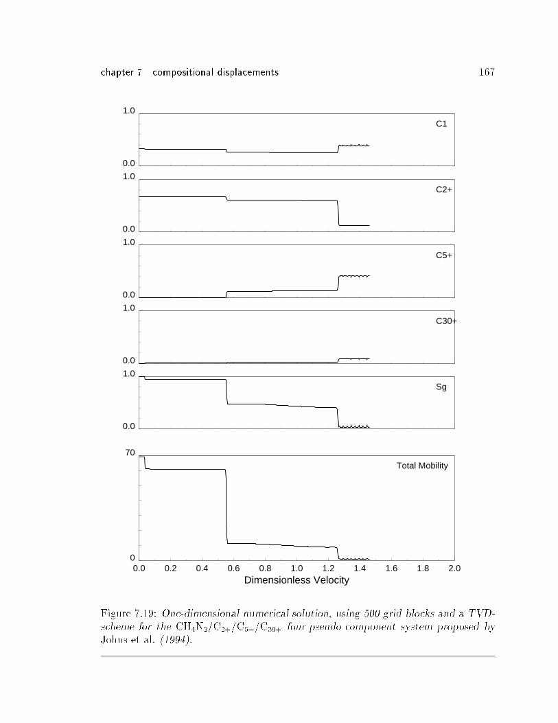
chapter 7 compositional displacements 167
0.0
1.0
0.0
1.0
0.0
1.0
0.0
1.0
0.0
1.0
0
70
0.0 0.2 0.4 0.6 0.8 1.0 1.2 1.4 1.6 1.8 2.0Dimensionless Velocity
C1
C2+
C5+
C30+
Sg
Total Mobility
Figure 7.19: One-dimensional numerical solution, using 500 grid blocks and a TVD-
scheme for the CH4N2=C2+=C5+=C30+ four-pseudo-component system proposed by
Johns et al. (1994).
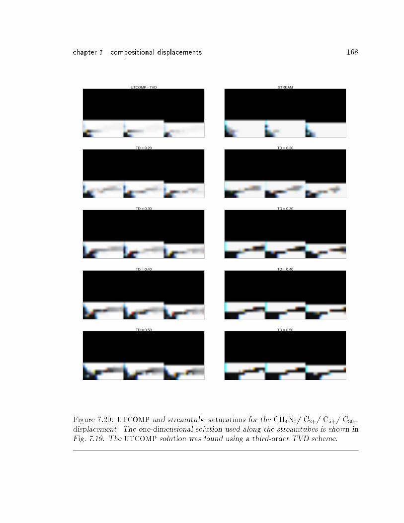
chapter 7 compositional displacements 168
UTCOMP - TVD
TD = 0.20
TD = 0.30
TD = 0.40
TD = 0.50
STREAM
TD = 0.20
TD = 0.30
TD = 0.40
TD = 0.50
Figure 7.20: UTCOMP and streamtube saturations for the CH4N2/ C2+/ C5+/ C30+
displacement. The one-dimensional solution used along the streamtubes is shown inFig. 7.19. The UTCOMP solution was found using a third-order TVD scheme.
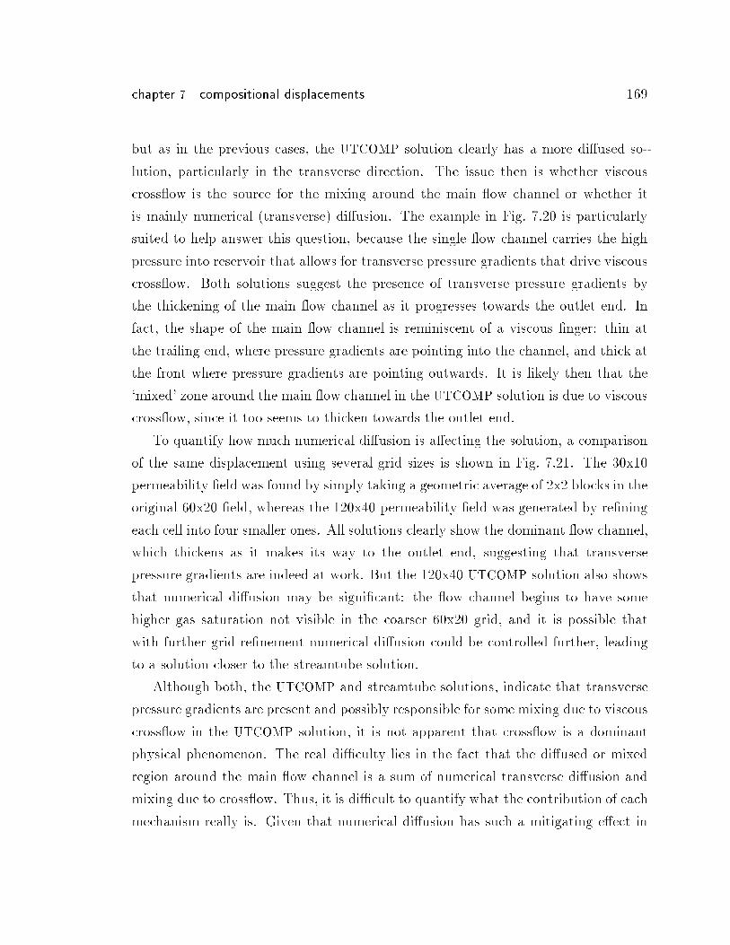
chapter 7 compositional displacements 169
but as in the previous cases, the UTCOMP solution clearly has a more di�used so-
lution, particularly in the transverse direction. The issue then is whether viscous
cross ow is the source for the mixing around the main ow channel or whether it
is mainly numerical (transverse) di�usion. The example in Fig. 7.20 is particularly
suited to help answer this question, because the single ow channel carries the high
pressure into reservoir that allows for transverse pressure gradients that drive viscous
cross ow. Both solutions suggest the presence of transverse pressure gradients by
the thickening of the main ow channel as it progresses towards the outlet end. In
fact, the shape of the main ow channel is reminiscent of a viscous �nger: thin at
the trailing end, where pressure gradients are pointing into the channel, and thick at
the front where pressure gradients are pointing outwards. It is likely then that the
`mixed' zone around the main ow channel in the UTCOMP solution is due to viscous
cross ow, since it too seems to thicken towards the outlet end.
To quantify how much numerical di�usion is a�ecting the solution, a comparison
of the same displacement using several grid sizes is shown in Fig. 7.21. The 30x10
permeability �eld was found by simply taking a geometric average of 2x2 blocks in the
original 60x20 �eld, whereas the 120x40 permeability �eld was generated by re�ning
each cell into four smaller ones. All solutions clearly show the dominant ow channel,
which thickens as it makes its way to the outlet end, suggesting that transverse
pressure gradients are indeed at work. But the 120x40 UTCOMP solution also shows
that numerical di�usion may be signi�cant: the ow channel begins to have some
higher gas saturation not visible in the coarser 60x20 grid, and it is possible that
with further grid re�nement numerical di�usion could be controlled further, leading
to a solution closer to the streamtube solution.
Although both, the UTCOMP and streamtube solutions, indicate that transverse
pressure gradients are present and possibly responsible for some mixing due to viscous
cross ow in the UTCOMP solution, it is not apparent that cross ow is a dominant
physical phenomenon. The real di�culty lies in the fact that the di�used or mixed
region around the main ow channel is a sum of numerical transverse di�usion and
mixing due to cross ow. Thus, it is di�cult to quantify what the contribution of each
mechanism really is. Given that numerical di�usion has such a mitigating e�ect in
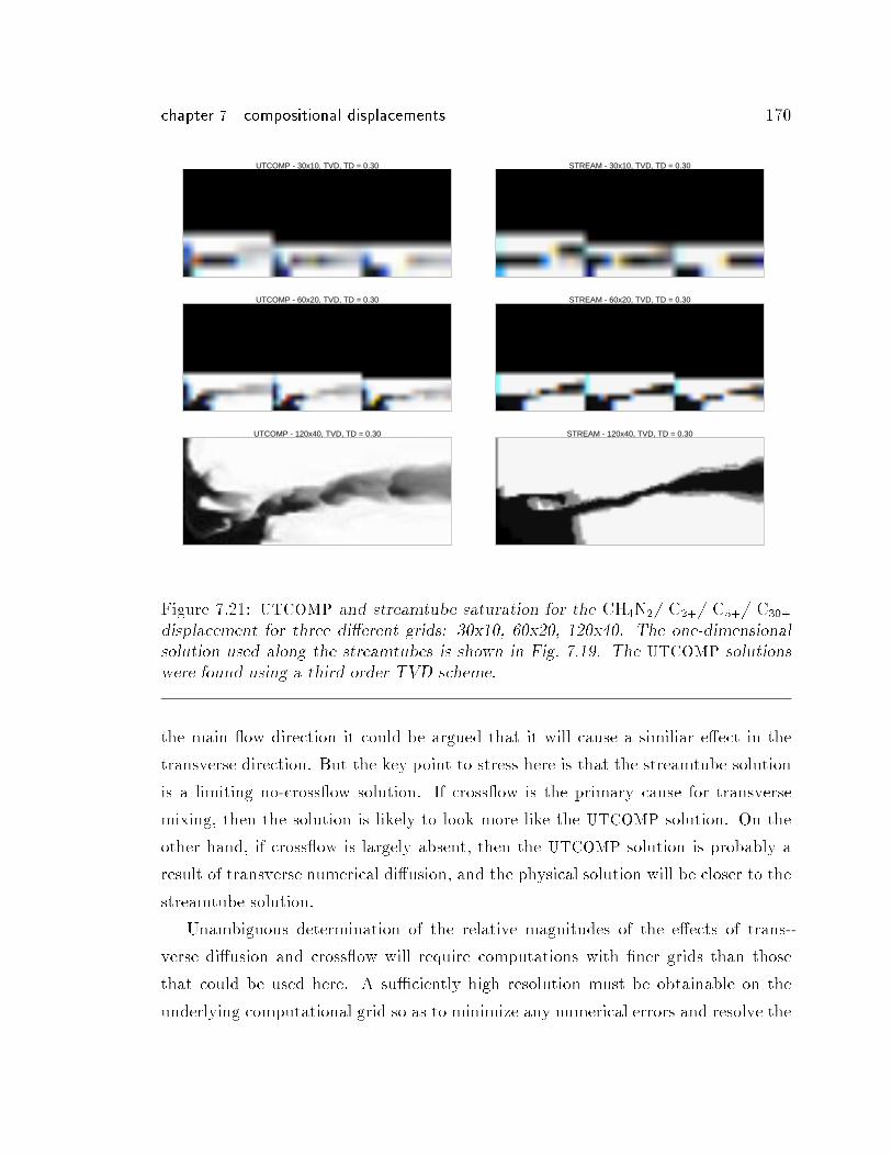
chapter 7 compositional displacements 170
UTCOMP - 30x10, TVD, TD = 0.30
UTCOMP - 60x20, TVD, TD = 0.30
UTCOMP - 120x40, TVD, TD = 0.30
STREAM - 30x10, TVD, TD = 0.30
STREAM - 60x20, TVD, TD = 0.30
STREAM - 120x40, TVD, TD = 0.30
Figure 7.21: UTCOMP and streamtube saturation for the CH4N2/ C2+/ C5+/ C30+
displacement for three di�erent grids: 30x10, 60x20, 120x40. The one-dimensionalsolution used along the streamtubes is shown in Fig. 7.19. The UTCOMP solutionswere found using a third order TVD scheme.
the main ow direction it could be argued that it will cause a similiar e�ect in the
transverse direction. But the key point to stress here is that the streamtube solution
is a limiting no-cross ow solution. If cross ow is the primary cause for transverse
mixing, then the solution is likely to look more like the UTCOMP solution. On the
other hand, if cross ow is largely absent, then the UTCOMP solution is probably a
result of transverse numerical di�usion, and the physical solution will be closer to the
streamtube solution.
Unambiguous determination of the relative magnitudes of the e�ects of trans-
verse di�usion and cross ow will require computations with �ner grids than those
that could be used here. A su�ciently high resolution must be obtainable on the
underlying computational grid so as to minimize any numerical errors and resolve the
chapter 7 compositional displacements 171
cross ow adequately. In that case, the impact of mixing due to cross ow could be
assessed by direct comparison with the streamtube solutions presented here. Thus,
the streamtube technique provides a basis for improved understanding of the e�ects
of cross ow, given that the current computational cost limits of compositional simu-
lations can be overcome.
7.8 Concluding Remarks
Unlike the previous chapters, the main issue raised here is not whether the stream-
tube approach can model compositional displacements, but rather how good tradi-
tional �nite di�erence solutions to compositional problems really are. The simple
and straightforward streamtube formulation is used to quantify numerical di�usion
and demonstrates that its continuous feed-back into the phase behavior computation
can substantially reduce the mobility contrast in a traditional �nite di�erence for-
mulation. In fact, the combination of numerical di�usion and phase behavior may
be so strong that doubling the number of grid blocks or using third-order numerical
schemes may simply not show substantial improvement in the solution, particularly
in retaining the unstable characteristic of the displacement | in other words, the
same numerical di�usion control that is achieved by doubling the grid blocks in a
�rst-contact miscible displacement may require tripling or quadrupling the number of
grid blocks for a compositional simulation. This type of numerical di�usion control,
while retaining an acceptable level of reservoir description, is currently not possible
with available computational resources. The streamtube approach is a simple and
robust alternative that can solve very large problems without losing the underlying
physics of the displacement to numerical di�usion and return a good approximation
of overall recovery in four to �ve orders of magnitude less time than traditional simu-
lation approaches. The streamtube solution cannot, by de�nition, model mixing due
to viscous cross ow, and thus represents a no-cross ow limit. If mixing due to viscous
cross ow is assumed to be a second-order e�ect, then the streamtube solution is a
reasonable approximation to the true solution of a compositional displacement.
Chapter 8
Summary and Conclusions
The main ideas and conclusions discussed in this dissertation are summarized, and
the limitations of the streamtube approach are reviewed.
8.1 Summary
The underlying assumption in applying the streamtube method to describe multi-
phase, multicomponent ow in heterogeneous porous media is that �eld scale dis-
placements are dominated by reservoir heterogeneity and convective forces. Flow
paths are captured by streamtubes, the geometry of which re ects the distribution
of high and low ow regions in the reservoir. Each streamtube is treated as a one-
dimensional system along which solutions to mass conservation equations for di�er-
ent displacement mechanisms can be mapped. The streamtube approach e�ectively
decouples the `channeling' imposed by the reservoir heterogeneity from the actual
displacement mechanism taking place. In other words, regardless of the displacement
type, the assumption is that there are prede�ned ow paths that will dominate the
two-dimensional solution. The uid velocity along these ow paths is re ected by the
geometry of the streamtubes, and the inherent nonlinearity in the underlying velocity
�eld is captured by periodically updating the streamtubes.
One-dimensional solutions are mapped along the streamtubes using a `Riemann
approach' | each streamtube is treated as a true one-dimensional system with con-
stant initial and injected conditions, allowing to time-step by integrating from tD = 0
172
chapter 8 summary and conclusions 173
to tD = tD + �tD. This approach allows analytical and numerical solutions to hy-
perbolic conservation equations (found using Riemann boundary conditions) to be
mapped along periodically updated streamtubes. The reason for using the Riemann
approach is to avoid di�culties associated with general-type initial conditions along
streamtubes, in which case solutions could be found only numerically for each time
step by either using a �nite-di�erence approach or a front-tracking type approach.
General-type initial conditions along streamtubes arise by updating the streamtubes
while keeping the spatial saturation/concentration/composition distribution �xed.
Initializing each new streamtube in this way produces initial conditions that are
problem speci�c and of general-type.
Solutions for (1) tracer ow, (2) two-phase immiscible ow, (3) �rst-contact misci-
ble ow, and (4) two-phase, multicomponent ow are found for a multitude of hetero-
geneous systems. For tracer ow the streamtubes are �xed in time and the Riemann
approach is equivalent to time stepping from tD to tD+�tD. The only assumption in
�nding two-dimensional solutions involves neglecting transverse di�usion/dispersion
mechanisms. In the limit of a piston-like front, a di�usion-free two-dimensional solu-
tion is found that can be used to quantify the error introduced by numerical di�usion
in traditional simulation methods. Longitudinal physical di�usion can be added ex-
plicitly by mapping a CD-solution for a given Peclet number along streamtubes. Using
the CD-solution is also an example of representing two di�erent scales of reservoir
heterogeneity: the large-scale heterogeneity captured by the geometry of the stream-
tubes and a smaller scale heterogeneity within each streamtube quanti�ed indirectly
by the Peclet number. The di�usive length scale associated with the choice of the
Peclet number also allows scaling of the two-dimensional solution.
In the two-phase immiscible case the velocity �eld becomes a function of satu-
ration and the streamtubes are updated periodically as the ood progresses. The
Riemann approach is used to map the Buckley-Leverett solution along streamtubes.
Evidence is presented to show that the error due to the Riemann approach is less than
the error introduced by numerical di�usion in a traditional �nite di�erence solution.
The key result, though, is the convergence of the streamtube approach with orders of
magnitude fewer matrix inversions (velocity �eld updates) than traditional solutions.
chapter 8 summary and conclusions 174
Only a few streamtube updates (less than 20 over 2 pore volumes injected) are nec-
essary to predict overall recovery correctly. The speed of the streamtube approach is
put to use by processing 60 geostatistical images to demonstrate the interaction of
nonlinearity and reservoir heterogeneity.
Applying the streamtube approach to �rst-contact miscible ow raises the chal-
lenging question of the `correct' one-dimensional solution to be used. Scaling ar-
guments are used to suggest that streamtubes that gave rise to a Fickian limit for
M = 1 displacements (tracer ow) should now see a viscous �ngering ow regime for
unstable M > 1 �rst-contact displacements. Thus, a Todd{Longsta� model is used
to capture the sub-streamtube viscous �ngering regime. Solutions are found using
a piston-like one-dimensional solution and a CD-solution along streamtubes as well,
although these solutions cannot be reconciled with the scale of the M = 1 solution.
The streamtube method is again able to predict recoveries using orders (2-3) of mag-
nitude less computation time than traditional simulation approaches. To demonstrate
the power of this approach, 180 recoveries are found to show how nonlinearity and
reservoir heterogeneity interact to de�ne the uncertainty in overall recovery, and the
usefulness of the streamtube approach as a fast �lter is pointed out. Only perme-
ability �elds returning maximum and minimum overall recoveries in the streamtube
approach need to be used to con�rm the spread in recovery using an expensive �nite
di�erence/�nite element simulation.
For compositional displacements the streamtube approach is shown to be partic-
ularly powerful due to its simplicity, robustness, and speed. The streamtube method
is used to assess how good traditional numerical solutions to compositional displace-
ments really are, particularly in view of interactions of numerical di�usion interacting
with phase behavior calculations. The key result is the demonstration that numerical
di�usion can substantially if not completely eliminate any mobility contrast in �nite
di�erence solutions. Streamtube solutions can be made to match �nite di�erence so-
lutions by simply using a unit mobility ratio calculation: mapping one-dimensional
composition pro�les along constant streamtubes. The resulting speed-up can range
from 3 to 5 order of magnitude. In traditional �nite di�erence simulation, convergence
of the solution by progressive grid re�nement is very slow, possibly requiring several
chapter 8 summary and conclusions 175
times (2-4) the number of grid re�nements used in FCM displacements to demon-
strate convergence. Finally, because mixing due to viscous cross ow and transverse
numerical di�usion result in the same e�ect, their individual contribution can not be
quanti�ed readily. The streamtube solution is, by de�nition, a solution that cannot
account for mixing due to viscous cross ow or transverse di�usion, and thus it repre-
sents a limiting solution where these mechanisms are assumed to have a second-order
e�ect.
8.2 Limitations of the Streamtube Approach
As with all numerical techniques, the streamtube approach discussed in this disser-
tation clearly has its limitations. In part, the limitations are connected to the one-
dimensional solutions used along the streamtube. The Riemann approach to mapping
one-dimensional solutions along periodically updated streamtubes centers on the as-
sumption of constant boundary conditions. If the boundary conditions change with
time, as may happen in an areal domain where wells are shut-in, new wells are in-
troduced, and ow rates vary, the Riemann approach may not work. Another key
assumption in the streamtube method is the dominance of the heterogeneity in de-
termining the ow response. If the reservoir is only mildly heterogeneous, though,
viscous �ngers, which the streamtube solution would fail to recognize, may actually
dominate the displacement mechanism. The streamtube approach is not able to rep-
resent any transverse ow mechanism that leads to mixing explicitly. Thus, transverse
di�usion and mixing due to viscous forces cannot be accounted for. Finally, account-
ing for gravity may not be as straightforward as modeling viscous forces, particularly
in multiphase ow, because now the velocity vectors for each phase do not point in
the direction of the total velocity.
8.3 Conclusions
The following main conclusions, in order of importance, are drawn from applying the
streamtube approach to modeling multiphase, multicomponent ow:
chapter 8 summary and conclusions 176
Fast, accurate, and robust solutions. The streamtube approach produces fast,
accurate, and robust solutions for displacements that are dominated by reser-
voir heterogeneity. Streamtube geometries capture the impact of heterogeneity
on the ow �eld, while the one-dimensional solutions mapped along them re-
tain the essential physics of the displacement mechanism. Speed-up is by two
to three orders of magnitude for two-phase immiscible and �rst-contact miscible
displacements and four to �ve orders for two-phase compositional displacements.
The absence of any convergence criteria and the ability to capture all the es-
sential physics of the displacement (like phase behavior) in the one-dimensional
solution leads to particularly robust solutions.
Statistical reservoir forecasting. The speed of the streamtube approach makes
it an ideal tool for statistical reservoir forecasting: hundreds of geostatistical
images can be processed in a fraction of the time required by traditional reser-
voir simulators. Applications to two-phase immiscible and �rst-contact misci-
ble displacements show a substantial uncertainty in overall recovery due to the
combined e�ects of reservoir heterogeneity and the inherent nonlinearity of the
displacements. As reservoir heterogeneity and nonlinearity increase so does the
uncertainty in overall recovery. The streamtube approach can be used to quan-
tify this uncertainty, which in turn can then be con�rmed by a more expensive
traditional approach using only the two geostatistical images that produces the
maximum and minimum recoveries. Although the streamtube method makes
strong assumptions in generating the two-dimensional solutions, the uncertainty
in recovery due to heterogeneity is shown to be substantially larger than the
error introduced by the Riemann approach.
Weak nonlinearity of . For all displacements, the necessary updates of the stream-
tubes to converge onto a solution are shown to be many orders of magnitude less
than the equivalent number of pressure solves in traditional numerical simula-
tion approaches. As a result, updating the streamtubes only periodically (20-40
times per 2 pore volumes injected) and using a one-dimensional solutions that
captures the essential physics of the displacement is su�cient to give accurate
chapter 8 summary and conclusions 177
overall recoveries.
Impact of numerical di�usion on compositional displacements. Numerical dif-
fusion is found to have a signi�cant role in reducing the mobility contrast in
traditional �nite di�erence solutions of compositional displacements. Compar-
ison of streamtube solutions to �nite di�erence solutions it is found that the
original mobility contrast is substantially reduced and even completely elimi-
nated by the presence of numerical di�usion. Streamtube solutions can be made
to match �nite di�erence solutions by simply using a unit mobility ratio pro�le.
Reservoir heterogeneity, phase behavior, and numerical di�usion are found to
be so dominant in compositional displacements that convergence due to pro-
gressive grid re�nement is very slow. Two to four times the re�nement used in
�rst-contact miscible displacements may be necessary in compositional displace-
ments, particularly if a single-point upstream weighting scheme is being used,
to see the equivalent improvement in the solution. As a result, compositional
displacements on coarse grids obtained using a single-point upstream weighting
scheme are not likely to result in converged solutions.
Decoupling of phase behavior from 2D grid. The streamtube approach is par-
ticularly powerful for multiphase compositional displacement. All the phase
behavior is now contained in the one-dimensional solution that is mapped along
the streamtubes, completely decoupling the underlying cartesian grid used to
specify reservoir heterogeneity from phase behavior considerations. This ap-
proach di�ers from traditional approaches to reservoir simulation, which per-
form a ash calculation for each grid block at each time step. As a result, the
streamtube approach makes for very robust solutions, particularly in the case
of compositional displacements.
Cross ow. Because mixing due to viscous cross ow and transverse numerical di�u-
sion result in the same e�ect, their individual contributions cannot be quanti�ed
readily. The streamtube solution is, by de�nition, a solution that cannot ac-
count for mixing due to viscous cross ow or transverse di�usion, and thus it
represents a limiting solution where these mechanisms are assumed to have a
chapter 8 summary and conclusions 178
second-order e�ect. The streamtube solutions provide a useful limiting case
against which the impact of cross ow can be measured.
Di�usion-free solutions. One-dimensional analytical solutions can be mapped along
streamtubes to obtain numerical-di�usion-free solutions. For tracer ow, the so-
lution is shown to be exact in the limit of in�nite streamtubes and benchmark
solutions can be generated in two dimensions, which can be used to test numer-
ical schemes.
Scale of 2D solutions. By mapping a convection-di�usion model or a viscous �n-
gering model an implicit assumption about the scale of the two-dimensional
solutions is made in �rst-contact miscible displacements. Sub-streamtube het-
erogeneities are assumed to lead to a Fickian limit for M = 1 displacements,
while giving rise to viscous �ngering ow regime for unstable M > 1 displace-
ments. Thus, the streamtube approach is an example of how physical phenom-
ena that take place at di�erent scales can be nested into a single model.
NOMENCLATURE
A area, or coe�cient
Ai cross section of ith streamtube
B coe�cient
C concentration, or coe�cient
CD dimensionless concentration
fw water fractional ow
HI heterogeneity index
h separation length of permeability values
i index, x-direction or streamtube; orp�1
j index, y-direction~~Kij di�usion/dispersion of component i in phase j, tensor
K di�usion/dispersion, constant
Km molecular di�usion~~k absolute permeability, tensor
kx absolute permeability in x-direction
ky absolute permeability in y-direction
krj relative permeability of phase j
L system length
Lrep representative di�usive length scale
M mobility ratio
Me� e�ective mobility ratio
Mend end-point mobility ratio
Mshock shock front mobility ratio
179
nomenclature 180
Mw molecular weight
N number of streamtubes
NX number of grid blocks in x-direction
NY number of grid blocks in y-direction
Np number of phases
NPe Peclet number
P pressure
Pc critical pressure
qi ow rate of ith streamtube
Q ow rate
Qtotal total ow rate
Sj saturation of phase j
Sw water saturation
s coordinate along a streamline
Tc critical temperature
TVD total variation diminishing
t time
tD dimensionless time
tDi dimensionless time of ith streamtube
uw;o water, oil Darcy velocity
uj Darcy velocity of phase j
ux Darcy velocity in the x-direction
uy Darcy velocity in the y-direction
Vc critical volume
VDP Dykstra{Parson coe�cient
VPi porevolume of ith streamtube
�VP porevolume used for scaling
vDi dimensionless velocity along ith streamtube
x Cartesian direction
xD dimensionless distance
xDidimensionless distance along ith streamtube
nomenclature 181
y Cartesian direction
yA y-coordinate of streamline A
yB y-coordinate of streamline B
Greek and symbols
�L,�T longitudinal and transverse dispersivity
�tD dimensionless time intervall
�x size of grid block in x-direction
�y size of grid block in y-direction,
or di�erence in y-coordinate of streamlines at a �xed x
� coordinate along streamtube/streamline
� mobility
�c correlation length of permeability �eld
�x mobility in the x-direction
�y mobility in the y-direction
�j viscosity of phase j
�w;o;s water, oil, solvent viscosity
�j density of phase j
� standard deviation
�lnK standard deviation of log-permeability distribution
� porosity
� potential function
streamfunction
complex potential
! Todd $ Longsta� parameter,
or acentric factor
!i mole fraction of component i
!ij mole fraction of component i in phase j
Bibliography
[1] Abbaszadeh-Dehghani, M.: Analysis of Unit Mobility Ratio Well-to-Well
Tracer Flow to Determine Reservoir Heterogeneity, PhD dissertation, Stan-
ford University (December 1982).
[2] Abramowitz, M. and Stegun, I.A.: Handbook of Mathematical Functions,
Dover (1970).
[3] Araktingi, U.G. and Orr, F.M., Jr.: \Viscous Fingering in Heterogeneous
Porous Media," Advanced Technology Series (October 1993) Vol.1, No.1,
71{80.
[4] Aris, R. and Amundson, N.: \Some Remarks on Longitudinal Mixing or Di�u-
sion in Fixed Beds," AIChe Journal (1957) 280.
[5] Arya, A., Hewett, T.A., Larson, R.G., and Lake, L.W.: \Dispersion and Reser-
voir Heterogeneity," SPE Reservoir Engineering (February 1988) 139{148.
[6] Aziz, K. and Settari, A.: Petroleum Reservoir Simulation, Applied Science
Publishers, Essex, England (1979).
[7] Bahralolom, I., Bretz, R.E. and Orr, F.M., Jr.: \Experimental Investigation
of the Interaction of Phase Behavior With Microscopic Heterogeneity in a CO2
Flood," Soc. Pet. Eng. J. (May 1988) 3, No. 2, 662{672.
[8] Bear, J.: Dynamics of Fluids in Porous Media, American Elsevier, New York
(1972).
182
BIBLIOGRAPHY 183
[9] Blackwell, R.: \Laboratory Studies of Microdispersion Phenomena," Society
of Petroleum Engineers Journal (March 1962) No. 1{8.
[10] Blackwell, R.J., Rayne, J.R. and Terry, W.M.: \Factors In uencing the E�-
ciency of Miscible Displacement," Trans., AIME (1959) 216, 1{8.
[11] Blunt, M.J. et al.: \Predictive Theory for Viscous Fingering in Compositional
Displacement," SPE Reservoir Engineering (February 1994) 9, No. 1, pp. 73{
80.
[12] Bommer, M.P. and Schechter, R.S.: \Mathematical Modeling of In-Situ Ura-
nium Leaching," Society of Petroleum Engineers Journal (December 1979)
393{400.
[13] Bratvedt, F., Bratvedt, K., Buchholz, C.F. et al.: \A New Front-Tracking
Method for Reservoir Simulation," paper SPE 19805 presented at the 1989 64th
SPE Annual Technical Conference and Exhibition, San Antonio, TX, October.
[14] Brigham, W.E., Reed, P.W., and Dew, J.N.: \Experiments on Mixing Dur-
ing Miscible Displacements in Porous Media," Society of Petroleum Engineers
Journal (March 1961) 1{8.
[15] Buckley, S.E. and Leverett, M.C.: \Mechanism of Fluid Displacement in
Sands," Trans., AIME (1941) 249, 107{116.
[16] Campbell, B. and Orr, F. J.: \Flow Visualization for CO2/Crude{Oil Displace-
ments," Society of Petroleum Engineers Journal (October 1985) 665{78.
[17] Chang, Y.-B.: Development of Three{Dimensional, Equation{of{State Com-
positional Reservoir Simulator for Miscible Gas Flooding, PhD dissertation,
The University of Texas at Austin (1990).
[18] Chang, Y.-B., Lim, M.T., Pope, G.A., and Sepehrnoori, K.: \CO2 Flow Pat-
terns Under Multiphase Flow: Heterogeneous Field Scale Conditions," SPE
Reservoir Engineering (August 1994) 208{216.
BIBLIOGRAPHY 184
[19] Chang, Y.-B., Pope, G.A., and Sepehrnoori, K.: \A Higher{Order Finite Dif-
ference Compositional Simulator," J. Phys. Sci. and Eng. (November 1990).
[20] Cheng, A.-D.: \Darcy's FlowWith Variable Permeability: A Boundary Integral
Solution," Water Resources Research (July 1984) 20, No. 7, 980{984.
[21] Christie, M.: \High Resolution Simulation of Unstable Flows in Porous Media,"
SPE Reservoir Engineering (1989) 4, No. 3, 297{303.
[22] Christie, M. and Bond, D.: \Multidimensional Flux{Corrected Transport for
Reservoir Simulation," paper SPE SPE 13505 presented at the 1985 Reservoir
Simulation Symposium, Dallas.
[23] Christie, M.A. and Bond, D.J.: \Detailed Simulation of Unstable Processes
in Miscible Flooding," Soc. Pet. Eng. Res. Eng. (November 1987) 2, No. 4,
514{522.
[24] Churchill, R. and Brown, J.: Complex Variables and Applications, �fth edition
edition, McGraw-Hill Publishing Company (1990).
[25] Courant, R., Friedrichs, K.O., and H. Lewy: \Ueber die partiellen Di�erenz-
gleichungen der mathematischen Physik," Math. Ann. (1928) 100, pp. 32{74.
[26] Dagan, G.: \Time{Dependent Macrodispersion for Solute Transport in
Anisotropic Heterogeneous Aquifers," Water Resources Research (September
1988) 24, No. 9, 1491{1500.
[27] Dake, L.P.: Fundamentals of Reservoir Engineering, Elsevier Scienti�c Pub-
lishing Company (1978).
[28] Deutsch, C.V. and Journel, A.G.: GSLIB Geostatistical Software Library and
User's Guide, Oxford University Press (1992).
[29] Dindoruk, B.: Analytical Theory of Multiphase, Multicomponent Displacement
in Porous Media, PhD dissertation, Stanford University, Stanford, CA (1992).
BIBLIOGRAPHY 185
[30] Dindoruk, B., Johns, R.T. and Orr, F.M., Jr.: \Analytical Solution for Four
Component Gas Displacements with Volume Change on Mixing," (June 1992)
Third European Conference on the Mathematics of Oil Recovery, Delft, Holland.
[31] Dougherty, E. and Sheldon, J.: \The Use of Fluid-Fluid Interfaces to Pre-
dict the Behavior of Oil Recovery Processes," Society of Petroleum Engineers
Journal (June 1964) 171{182.
[32] Dougherty, E.L.: \Mathematical Model of an Unstable Miscible Displacement,"
Soc. Pet. Eng. J. (June 1963) 155{163.
[33] Douglas, J., Peaceman, D.W., and Rachford, H.H.: \A Method for Calculating
Multi-Dimensional Immiscible Displacement," Trans. AIME (1959) 216.
[34] Doyle, R.E. and Wurl, T.M.: \Stream Channel Concept Applied to Water ood
Performance Calculations For Multiwell, Multizone, Three-Component Cases,"
Journal of Petroleum Technology (March 1971) 373{380.
[35] Emanuel, A.S., Alameda, G.K., Behrens, R.A., and Hewett, T.A.: \Reser-
voir Performance Prediction Methods on Fractal Geostatistics," SPE Reservoir
Engineering (August 1989) 311{318.
[36] Evans, D. and Ra�ensperger, J.: \On the Stream Function for Variable-Density
Groundwater Flow," Water Resources Research (August 1992) 28, No. 8, 2141{
2145.
[37] Ewing, R.E, Russell, T.F., and Wheeler, M.F.: \Simulation of Miscible Dis-
placement Using Mixed Methods and a Modi�ed Method of Characteristics,"
paper SPE 12241 presented at the 1983 Reservoir Simulation Symposium, San
Francisco, CA, November.
[38] Fayers, F. and Lee, S.: \Cross ow Mechanisms In Oil Displacements By Gas
Drive In Heterogeneous Reservoirs," In Situ (1994) 18, No. 4.
BIBLIOGRAPHY 186
[39] Fayers, F.J.: \An Approximate Model with Physically Interpretable Parame-
ters for Representing Miscible Viscous Fingering," SPE Reservoir Engineering
(May 1988) 3, 551{558.
[40] Fayers, F.J., Al�eonard, B., and Jouaux, F.: \Progress with Compositional
Studies in Heterogeneous Systems for Slightly Submiscible Gas Displacements,"
paper SPE SPE 27832 presented at the 1994 DOE/SPE Improved Oil Recovery
Symposium, Tulsa, Oklahoma, April 17{20.
[41] Fayers, F.J., Blunt, M.J. and Christie, M.A.: \Comparison of Empirical Vis-
cous Fingering Models and Their Calibration for Heterogeneous Problems,"
SPE Reservoir Engineering (May 1992) 195{202.
[42] Frind, E. and Matanga, G.: \The Dual Formulation of Flow for Contami-
nant Transport Modeling 1. Review of Theory and Accuracy Aspects," Water
Resources Research (February 1985) 21, No. 2, 159{169.
[43] Frind, E.O., Matanga, G.B., and Cherry, J.A.: \The Dual Formulation of Flow
for Contaminant Transport Modeling 2. The Borden Aquifer," Water Resources
Research (February 1985) 21, No. 2, 170{182.
[44] Gardner, J.W. and Ypma, J.G.J.: \An Investigation of Phase-
Behavior/Macroscopic-Bypassing Interaction in CO2 Flooding," Soc. Pet. Eng.
Journal (October 1984) 508{520.
[45] Gelhar, L.: Stochastic Subsurface Hydrology, Prentice Hall (1993).
[46] Gelhar, L.W. and Axness, C.L.: \Three-Dimensional Stochastic Analysis of
Macrodispersion in Aquifers," Water Resources Research (1983) 19, No. 1,
161{180.
[47] Glimm, J., Lindquist, B., McBryan, O.A., Plohr, B., and Yaniv, S.: \Front
Tracking for Petroleum Simulation," paper SPE 12238 presented at the 1983
Reservoir Simulation Symposium, San Francisco, CA, November.
BIBLIOGRAPHY 187
[48] Gorell, S.: \Outlook for Calibration of Large Grid{Block Models for Miscible
Flooding Applications," paper SPE 24186 presented at the 1992 1992 SPE/DOE
Eight Symposium on Enhanced Oil Recovery, Tulsa, OK, April.
[49] Hauber, W.C.: \Prediction of Water ood Performance for Arbitrary Well Pat-
terns and Mobility Ratios," Journal of Petroleum Technology (January 1964)
94{103.
[50] Hewett, T. and Behrens, R.: \Scaling Laws in Reservoir Simulation and Their
Use in a Hybrid Finite Di�erence/Streamtube Approach to Simulation the Ef-
fects of Permeability Heterogeneity," Reservoir Characterization, II, L. Lake
and J. Carroll, H.B. (eds.), Academic Press, Inc., London (1991).
[51] Higgins R.V. and Leighton, A.J.: \A Computer Method to Calculate Two{
Phase Flow in Any Irregularly Bounded Porous Medium," Journal of Petroleum
Technology (June 1962) 679{683.
[52] Higgins R.V. and Leighton, A.J.: \Computer Prediction of Water Drive of Oil
and Gas Mixtures Through Irregularly Bounded Pororus Media | Three-Phase
Flow," Journal of Petroleum Technology (September 1962) 1048{1054.
[53] Higgins, R.V., Boley, D.W., and A.J. Leighton: \Aids to Forecasting The
Performance of Water Floods," Journal of Petroleum Technology (September
1964) 1076{1082.
[54] Johns, R.T.: Analytical Theory of Multicomponent Gas Drives With Two-
Phase Mass Transfer, PhD dissertation, Stanford University, Stanford, CA
(1992).
[55] Johns, R.T., B. Dindoruk, and Orr, F.M. Jr.: \Analytical Theory of Combined
Condensing/Vaporizing Gas Drives," paper SPE 24112 presented at the 1992
SPE/DOE Eighth Symposium on Enhanced Oil Recovery, Tulsa, OK, April.
[56] Johns, R.T., B. Dindoruk, and Orr, F.M. Jr.: \Analytical Theory of Combined
Condensing/Vaporizing Gas Drives," SPE Advanced Technology Series (May
1993) 1, No. 2, 7{16.
BIBLIOGRAPHY 188
[57] Johns, R.T., Fayers, F.J. and Orr, F.M., Jr.: \E�ect of Gas Enrichment
and Dispersion on Nearly Miscible Displacements in Condensing/Vaporizing
Drives," SPE Advanced Technology Series (1994) 2, No. 2, 173{180.
[58] King, M.J., Blunt, M.J., Mans�eld, M., and Christie, M.A.: \Rapid Evaluation
of the Impact of Heterogeneity on Miscible Gas Injection," paper SPE 26079
presented at the 1993 Western Regional Meeting, Anchorage.
[59] Koval, E.J.: \A Method for Predicting the Performance of Unstable Miscible
Displacements in Heterogeneous Media," Soc. Pet. Eng. J. (June 1963) 145{
154.
[60] Lafe, O. and Cheng, A.-D.: \A Perturbation Boundary Element Code for
Steady State Groundwater Flow in Heterogeneous Aquifers," Water Resources
Research (June 1987) 23, No. 6, 1079{1084.
[61] Lafe, O.E., Ligget, J.A., and Liu, P.L-F.: \BIEM Solutions to Combinations
of Leaky, Layered, Con�ned, Uncon�ned, Nonisotropic Aquifers," Water Re-
sources Research (October 1981) 17, No. 5, 1431{1444.
[62] Lake, L.W., Johnston, J.R., and Stegemeier, G.L.: \Simulation and Perfor-
mance Prediction of a Large-Scale Surfactant/Polymer Project," Society of
Petroleum Engineers Journal (December 1981) 731{739.
[63] Lake, W.L.: Enhanced Oil Recovery, �rst edition, Prentice Hall, Engelwood
Cli�s, NJ 07632 (1989).
[64] LeBlanc, J.L. and Caudle, B.H.: \A Streamline Model for Secondary Recovery,"
Society of Petroleum Journal (March 1971) 7{12.
[65] Lee, B.: \Potentiometric-model Studies of Fluid Flow in PetroleumReservoirs,"
Trans. AIME (1948) 174, 41.
[66] Lee, S-T, Lo, H. and Dharmawardhana, B.T.: \Analysis of Mass Transfer
Mechanisms Occurring in Rich Gas Displacement Process," paper SPE 18062
BIBLIOGRAPHY 189
presented at the 1988 SPE Annual Technical Conference and Exhibition, Hous-
ton, TX, October 2-5.
[67] LeVeque, R. J.: Numerical Methods for Conservation Laws, Birkhaeuser Verlag
(1992).
[68] Lin, J.: An Image Well Method for Bounding Arbitrary Reservoir Shapes in
the Streamline Model, PhD dissertation, U. of Texas , Austin (December 1972).
[69] Liu, P.L-F., Cheng A.H-D., Ligget J.A., and Lee, J.H.: \Boundary Integral
Equation Solutions to Moving Interface Between Two Fluids in Porous Media,"
Water Resources Research (October 1981) 17, No. 5, 1445{1452.
[70] Martin, J.C. and Wegner, R.E.: \Numerical Solution of Multiphase, Two-
Dimensional Incompressible Flow Using Streamtube Relationships," Society of
Petroleum Engineers Journal (October 1979) 313{323.
[71] Martin, J.C., Woo, P.T., and Wegner, R.E.: \Failure of Stream Tube Meth-
ods To Predict Water ood Performance of an Isolated Inverted Five-Spot at
Favorable Mobility Ratios," Journal of Petroleum Technology (February 1973)
151{153.
[72] Masukawa J. and Horne, R.N.: \Application of the Boundary Integral Method
to Immiscible Displacement Problems," SPE Reservoir Engineering (August
1988) 1069{1077.
[73] Matanga, G.: \Stream Functions in Three-Dimensional Groundwater Flow,"
Water Resources Research (September 1993) 29, No. 9, 3125{3133.
[74] Matheron, G. and de Marsily, G.: \Is Transport in Porous Media Always
Di�usive? A Counterexample.," Water Resources Research (1980) 16, No. 5,
901{9177.
[75] Mathews, J.L., Emanuel, A.S., and Edwards, K.A.: \Fractal Methods Improve
Mitsue Miscible Predictions," Journal of Petroleum Technology (November
1989) 1136{1989.
BIBLIOGRAPHY 190
[76] Mishra, S.: On the Use of Pressure and Tracer Test Data for Reservoir De-
scription, PhD dissertation, Stanford University, Stanford, CA (1987).
[77] Monroe, W.W.: \The E�ects of Dissolved Methane on Composition Paths in
Quaternary CO2-Hydrocarbon Systems," Master's thesis, Stanford University,
Stanford, CA (August 1986).
[78] Monroe, W.W., Silva, M.K., Larsen, L.L. and Orr, F.M. Jr.: \Composition
Paths in Four-Component Systems: E�ect of Dissolved Methane on 1D CO2
Flood Performance," Soc. Pet. Eng. Res. Eng. (August 1990) 423{432.
[79] Morel-Seytoux, H.: \Analytical-Numerical Method in Water ooding Predic-
tions," Society of Petroleum Engineers Journal (September 1965) 247{258.
[80] Muskat, M.: Flow of Homogeneous Fluids, International Human Resources
Development Corporation, 137 Newbury Street, Boston MA 02116 (1937, 1982).
[81] Muskat, M.: \The Theory of Potentiometric Models," Trans. AIME (1948)
179, 216{221.
[82] Muskat, M. and Wycko�, R.: \A Theoretical Analysis of Water ooding Net-
works," Trans. AIME (1934) 107, 62{77.
[83] Nelson, R.: \Evaluating the Environmental Consequences of Groundwater Con-
tamination 2. Obtaining Location/Arrival Time and Location/Out ow Quan-
tity Distributions for Steady Flow Systems," Water Resources Research (March
1978) 14, 416{428.
[84] Neuman, S.: \Universal Scaling of Hydraulic Conductivities and Dispersivities
in Geologic Media," Water Resources Research (August 1990) 26, No. 8, 1749{
1758.
[85] Newley, T.M.J. and Merrill R.C. Jr.: \Pseudocomponent Selection for Com-
positional Simulation," Soc. Pet. Eng. Res. Eng. (November 1991) 6, No. 4,
490{496.
BIBLIOGRAPHY 191
[86] Numbere, D. and Tiab, D.: \An Improved Streamline-Generating Technique
That Uses the Boundary (Integral) Element Method," SPE Reservoir Engi-
neering (August 1988) 1061{1068.
[87] Orr, F.M., Jr., Johns, R.T. and Dindoruk, B.: \Miscibility in Four-Component
Vaporizing Gas Drives," paper SPE 22637 presented at the 1991 SPE Annual
Technical Conference and Exhibition, Dallas, TX, October 6{9.
[88] Orr, F.M., Jr., Johns, R.T. and Dindoruk, B.: \Miscibility in Four-Component
Vaporizing Gas Drives," Soc. Pet. Eng. Res. Eng. (1993) 8, No. 28, 135{142.
[89] Pande, K.: \E�ects of Gravity and Viscous Cross ow on Hydrocarbon Mis-
cible Flood Performance in Heterogeneous Reservoirs," paper SPE SPE 24935
presented at the 1992 67th Annual Technical Conference and Exhibition, Wash-
ington, DC, October 4{7.
[90] Pande, K.K. and Orr, F.M., Jr.: \Interaction of Phase Behavior, Reservoir
Heterogeneity and and Cross ow in CO2 Floods," paper SPE 19668 presented
at the 1989 SPE Annual Technical Conference and Exhibition, San Antonio,
TX, October 8{11.
[91] Parsons, R.W.: \Directional Permeability E�ects in Developed and Uncon�ned
Five-Spots," Journal of Petroleum Technology (April 1972) 487{494.
[92] Peng, D.Y. and Robinson, D.B.: \A New Two-Constant Equation of State,"
Ind. Eng. Chem. Fund. (1976) 15, 59{64.
[93] Perkins, T. and Johnston, O.: \A Review of Di�usion and Dispersion in Porous
Media," SPEJ (March 1963) No. 3, 70{80.
[94] Renard, G.: \A 2D Reservoir Streamtube EOR Model with Periodical Auto-
matic Regeneration of Streamlines," In Situ (1990) 14, No. 2, 175{200.
[95] Sato, K.: Accelerated Perturbation Boundary Element Model for Flow Prob-
lems in Heterogeneous Reservoirs, PhD dissertation, Stanford University
(1992).
BIBLIOGRAPHY 192
[96] Sato, K. and Horne, R.: \Perturbation Boundary Element Method for Hetero-
geneous Reservoirs: Partt 1 | Steady-State Flow Problems," SPE Formation
Evaluation (December 1993) 306{314.
[97] Sato, K. and Horne, R.: \Perturbation Boundary Element Method for Het-
erogeneous Reservoirs: Part 1 | Transient-Flow Problems," SPE Formation
Evaluation (December 1993) 315{322.
[98] Sato, K. and Abbaszadeh, M.: \Complex Variable Boundary Element Method
fo Tracking Streamlines across Fractures," Proc. of the 4th European Con-
ference on the Mathematics of Oil Recovery, Roros, Norway (June 7{10 1994)
Topic D.
[99] Sheldon, J. and Dougherty, E.: \A Numerical Method for Computing the
Dynamical Behavior of Fluid-Fluid Interfaces in Permeable Media," Society of
Petroleum Engineers Journal (June 1964) 158{170.
[100] Sorbie, K.S., Feghi, F., Pickup, G.E., Ringrose, P.S., and Jensen J.L.:
\Flow Regimes in Miscible Displacement in Heterogeneous Correlated Random
Fields," paper SPE 24140 presented at the 1992 SPE/DOE Eighth Symposium
on Enhanced Oil Recovery, Tulsa, OK, April.
[101] Stalkup, F.I.: \Miscible Displacement," Monograph 8, Soc. Pet. Eng. of AIME,
New York (1983).
[102] Stalkup, F.I.: \Displacement Behavior of the Condensing/Vaporizing Gas
Drive Process," paper SPE 16715 presented at the 1987 SPE Annual Technical
Conference and Exhibition, Dallas, TX, September.
[103] Strack, O.: Groundwater Mechanics, Prentice Hall, Englewood Cli�s (1989).
[104] Tang, R.W., Behrens, R.A., Emanuel, A.S.: \Reservoir Studies Using Geo-
statistics To Forecast Performance," paper SPE 18432 presented at the 1989
SPE Symposium on Reservoir Simulation, Houston, TX.
BIBLIOGRAPHY 193
[105] Tchelepi, H.: Viscous Fingering, Gravity Segregation, and Permeability Hetero-
geneity in Two-Dimensional and Three-Dimensional Flows, PhD dissertation,
Stanford University (March 1994).
[106] Todd, M.R. and Longsta�, W.J.: \The Development, Testing and Application
of a Numerical Simulator for Predicting Miscible Flood Performance," Trans.,
AIME, 253 (1972) 874{882.
[107] UTCOMP{3.2: An Equation of State Compositional Simulator, Center for
Petroleum and Geosystems Engineering, University of Texas at Austin, TX
78712 (May 1993).
[108] Waggoner, J.R., Castillo, J.L., and Lake, L.W.: \Simulation of EOR Processes
in Stochastically Generated Permeable Media," Soc. Pet. Eng. Formation Eval.
(June 1992) 173{180.
[109] Walsh, B.W. and Orr, F.M. Jr.: \Prediction of Miscible Flood Performance:
The E�ect Of Dispersion on Composition Paths in Ternary Systems.," IN SITU
(1990) 14, No. 1, 19{47.
[110] Wang, B., Lake, L.W., and Pope, G.A.: \Development and Application of a
Streamline Micellar/Polymer Simulator," paper SPE 10290 presented at the
1981 56th Annual Fall Technical Conference and Exhibition, San Antonio, TX.
[111] Wattenbarger, R.: Simulation of Tracer Flow Through Heterogeneous Porous
Media, PhD dissertation, Stanford University (1993).
[112] Yih, C.: \Stream Functions in Three-Dimensional Flow," La Houille Blanche
(1957) 3, 445{450.
[113] Zauderer, E.: Partial Di�erential Equations of Applied Mathematics, second
edition, Wiley-Interscience, New York, NY (1989).
[114] Zick, A.A.: \A Combined Condensing/Vaporizing Mechanism in the Displace-
ment of Oil by Enriched Gas," paper SPE 15493 presented at the 1986 SPE
Annual Technical Conference and Exhibition, New Orleans, LA, October.
BIBLIOGRAPHY 194
[115] Zijl, W.: \Numerical Simulations Based on Stream Functions and Velocities in
Three-Dimensional Groundwater Flow," J. Hydrol. (1986) 85, 349{365.
Appendix A
Generating Permeability Fields
Although many sophisticated techniques exist to generate correlated permeability
�elds (Deutsch and Journel, 1992), a moving window method is used in this thesis
because of its simplicity and robustness. The underlying assumption is that the
permeability k is log-normally distributed. Thus, the probability that ln k is less
than or equal to some values x is given by
P (x) =1
�p2�
Zx
�1
e�(t��)2
2�2 dt ; (A:1)
where � and �2 are the average and variance respectively of the random variable
x = ln k. The algorithm is as follows.
1. Setting up the grid. If the desired reservoir is to have NX by NY grid blocks,
then the actual grid used to �nd the correlated �eld must have (NX + IX) by
(NY + IY ) blocks, where (IX ��x) and (IY ��y) are greater than or equal
to the radii in the x- and y-directions of the moving window. �x is and �y
specify the size of each grid block. This will assure that all (NX �NY ) blocks
will be assigned an average value calculated from the same number of points.
2. Generating a spatially random uniform distribution. The easiest way to
accomplish this is to simply draw (NX+IX)� (NY +IY ) random values from
the closed interval [0; 1] and assign them sequentially to each grid block. In fact,
it is better to generate a uniform distribution by picking (NX+IX)�(NY +IY )
195
appendix a generating permeability �elds 196
equally spaced values from the open interval (0; 1) and assigning them randomly
to the grid blocks. The advantage is that the underlying distribution will always
be symmetrical and independent from the random number generator. The ran-
dom number is only used to pick a random location in space, but the numerical
value of the random number is discarded.
3. Normal transformation. This step is not strictly necessary, but it does add
clarity to the method and is therefore presented here. With all blocks having
been assigned a value between zero and one, the underlying uniform distribution
is transformed to a standardized normal distribution (� = 0; � = 1) by using
the inverse of the cumulative distribution function. Recall that the standardized
cumulative distribution function is de�ned as
�(u) =1p2�
Zu
�1
e�t2
2 dt : (A:2)
Thus, for each point xi from the uniform distribution a point ui is found from
ui = ��1(xi) : (A:3)
The inversion, of course, is done numerically. A good source for expressions
approximating � and ��1 is Abramovitz and Stegun (1970).
4. Moving window. With the underlying distribution now being normal, but ran-
domly distributed, an ellipse is used as a moving window to �nd the correlated
�eld. The value for each block (�ui) is found by simply centering the ellipse on
the grid block and averaging all values (ui) that fall within the ellipse. The
resulting spatial correlation will then have a range equal to the diameters of
the ellipse. The resulting �eld is still normally distributed but with a standard
deviation less then one (�0 < 1) and a mean very close to zero (�0 � 0).
5. Transforming to absolute permeability. Finally, the averaged �eld is scaled
such that it has the desired standard deviation, or order of magnitude variation,
and average. If the average �eld values of part 4 are denoted by �ui and have
an average and standard deviation given by �� and �� then the transformation is
appendix a generating permeability �elds 197
given byln ki � �lnk
�ln k=
�ui � ��
��; (A:4)
where �ln k and �ln k and the desired values for the permeability �eld. The actual
permeability values are therefore found using
ki = exp��ln k
��(�ui � ��)
�+ �ln k : (A:5)
Appendix B
Summaries of Relevant Papers
Muskat and Wycko�, 1932: A Theoretical Analysis of Water ooding Networks
In this paper Muskat and Wycko� investigate the recovery e�ciency of well patterns using stream-lines. Using an electrical conduction model, they consider a staggered line drive, a direct line drive,a �ve-spot, and a seven-spot. The reservoir is considered homogeneous and tracer- ow assumptionsare used for all calculations (although they discuss their results in terms of multi-phase ow). Theyconclude that the staggered line drive has `the most favorable physical features'. It is interesting tonote though, that Muskat and Wycko� conclude their discussion by suggesting that well spacing andarrangement may be of minor importance compared to the channeling caused by `high permeabilityzones within the main body of sand'.Contribution: Quantifying ood e�ciencies of four di�erent well patterns using streamtubes.
Higgins and Leighton, 1962 (11/61)1: A Computer Method to Calculate Two-Phase Flow in Any
Irregularly Bounded Porous Medium
This paper is generally considered as being the �rst to introduce streamtubes to model two-phase ow in porous media. Higgins and Leighton acknowledge that complex well spacing have beenstudied using `potentiometric' models before, but point out that these considered single phase owonly. They test their two-phase approach for a �ve-spot against laboratory water oods reported byDouglas et al. (1959) as well as their `long method' for end-point viscosity ratios ranging from 0.083to 754. They report good matches, though it is important to note that the relative permeabilitycurves they used (`permeability-saturation curves') give rise to rarefaction waves only. The Higginsand Leighton method divides streamtubes into `sand elements' of equal volume. At the end of eachtime step, the average mobility (actually referred to as average permeability in the paper) and geo-metric shape factor are calculated for each sand element. The total resistance along each streamtube(`channel') is then used to �nd the instantaneous ow rate. The streamtubes are calculated onlyones using a single phase formulation and the reservoir is assumed homogeneous.Contribution: Two-phase ow solution accounting for changing mobility distribution along stream-tubes.
Higgins and Leighton, 1962 (4/62): Computer Predictions of Water Drive of Oil and Gas Mixtures
Through Irregularly Bounded Media{Three Phase Flow
1The date in parentheses indicates when the work was �rst presented.
198
appendix b summaries of relevant papers 199
In this paper, Higgins and Leighton extend their streamtube method to three phase ow. The one-dimensional, three-phase ow solution is constructed by using the water-oil fractional ow to �ndthe two-phase mixed-wave solution and having the displaced oil and gas move ahead of the front byassuming that no oil is displaced by the mobile gas. By considering several non-communicating layersolutions, each of which can have di�erent petrophysical properties, Higgins and Leighton show agood match for a particular �eld case.Contribution:Three-phase ow solution along streamtubes.
Hauber, 1964: Prediction of Water ood Performance for Arbitrary Well Patterns and Mobility Ra-
tios
Hauber presents general expressions for determining injectivity, time, and cumulative water injectedwhen the water-oil interface has moved a given distance along a streamtube. He introduces a distor-tion factor for non-unit mobility ratio displacements to account for changing streamtube geometriesas the ood progresses. Although the title of this paper is promising and Hauber indeed presents arather `mathematical' approach, it is di�cult to follow his derivations, in part due to the confusingnotation.Contribution: Analytical expressions to calculate injectivity, time, and cumulative water injectedfor an arbitrary streamtube.
Higgins, Boley, and Leighton, 1964 (5/64): Aids to Forecasting the Performance of Water Floods
In this paper Higgins et al. extend their method presented in 1962 to a seven-spot, a direct line-drive, and a staggered line-drive. The �ve-spot results �rst presented in 1962 are given as well. Inall cases the reservoir is considered homogeneous and streamtubes are calculated only once using thesingle phase assumption. Five streamtubes with 40 cells each were used for each symmetry elementin the patterns investigated. In this paper Higgins et al. conclude that phase mobilities (Higginset al. call them permeabilities) have a greater in uence on oil recovery than well spacing patterns.Although never mentioned explicitly, it appears that they used straight line relative permeabilitycurves leading, as in their 1962 paper, to rarefaction waves only. It is interesting to note that theyalso brie y touch on how an unfavorable vertical permeability pro�le can be a dominating factor onrecovery but do not elaborate.Contribution: Extension of streamtube approach to di�erent well patterns.
Doyle and Wurl, 1971 (10/69): Stream Channel Concept Applied to Water ood Performance Cal-
culations For Multiwell, Multizone, Three-Component Cases
In this paper Doyle and Wurl extend the Higgins and Leighton streamtube approach to �elds thathave a non-regular well pattern. Streamtubes (`channels') are generated for the entire �eld and allnecessary information stored for each channel to allow displacement calculations. An example �eldapplication is presented. Although Doyle and Wurl do not present any substantially new idea, thepaper conveys the simple and straightforward ideas of the streamtube approach though its clearexposition.Contribution: Application of streamtube solution to non-symmetrical well patterns.
LeBlanc and Caudle, 1971 (5/70): A Streamline Model for Secondary Recovery
This paper is, in essence, a rewrite of the original 1962 Higgins and Leighton paper, but improves onthe mathematical formulation of the problem. LeBlanc and Caudle generate the streamlines usingsuperposition and explicitly write-out the expressions for the x and y velocity components, somethingHiggins and Leighton in fact never did. They also mention that each streamtube will see an equalinjected volume for the unit mobility case, thus eliminating any need of geometrical information
appendix b summaries of relevant papers 200
about the streamtube. LeBlanc and Caudle use the center streamline for all their calculations. Buttheir claim of not having to know the entire streamlines is unsubstantiated . Although true for thelimiting unit mobility case, in all other cases they rely on the unit mobility streamlines (and thuson knowledge about the entire ow �eld) to �nd the total resistance down each tube.Contribution: Eliminating Higgins and Leighton geometrical shape factors.
Martin, Woo, and Wegner, 1973 (2/73): Failure of Stream Tube Methods to Predict Water ood
Performance of an Isolated Five-Spot at Favorable Mobility Ratios
In this letter to JPT, Martin et al. argue that for favorable mobility ratios the streamtube approachunderestimates recovery due the fact that the streamlines in the watered-out region are almostindependent of the high-mobility region ahead of the water bank. They show that a better solutionis obtained by updating the tubes several times as the ood progresses. A nice graph is presentedshowing the constant streamlines compared to the streamlines recalculated at some later time. Theidea is to recalculate the streamtubes, locate the old saturations onto the new streamtubes, andcontinue the displacement calculations.Contribution: Quantifying the error due to the constant streamtube assumption. Show improvedrecovery prediction by updating streamtube periodically.
Parsons, 1972 (10/71): Directional Permeability E�ects in Developed and Uncon�ned Five-Spots
In this paper Parsons investigates the e�ect of directional permeability on unit mobility displace-ments using streamlines. Contrary to previous authors, Parsons accumulates a `time-of- ight' alongstreamlines, with equal time-of- ight points on di�erent streamlines delineating a ood front. Par-sons presents a number of streamline maps for di�erent maximum permeability directions andanisotropy ratios and clearly shows that anisotropy can substantially a�ect the displacement process.This is particularly true for uncon�ned patterns.Contribution: Investigation of the e�ect of areal anisotropy in permeability on recovery for unitmobility displacements. Use of a time-of- ight coordinate.
Martin and Wegner, 1979 (4/78): Numerical Solution of Multiphase, Two-Dimensional Incompress-
ible Flow Using Stream-Tube Relationships
In this paper Martin and Wegner quantify the error caused by the assumption of �xed streamtubes.Although their title contains the word multi-phase, they only consider the two-phase immisciblewater ood problem. By investigating mobility ratios ranging from 0:1 to 1000, they demonstratethat the largest error occurs for favorable mobility ratios. They correctly attribute this to the largemobility decrease across the water bank in the M = 0:1 case. It should be noted though, that therelative permeabilities used by Martin and Wegner give rise to pure rarefaction waves in all unfa-vorable mobility ratio cases. Finally, it is interesting to note that they mention how the problem ofnumerical di�usion can be overcome using streamtubes. Unfortunately, they never actually quantifythis advantage of the streamtube approach.Contribution: Investigation of the error caused by the �xed streamtube assumption.
Bommer and Schechter, 1979 (10/78): Mathematical Modeling of In-Situ Uranium Leaching
This paper is an interesting application of the streamtube method to uranium leaching. In particular,the single phase, unit mobility type displacement involved in this application justi�es the constantstreamtube assumption. A component balance accounting for chemical reactions and physical dif-fusion is then solved by �nite-di�erences along each streamtube. The area of interest is boundedthrough the use of image wells which are placed using an algorithm developed by (Lin)1972. Thisalgorithm is not discussed in the paper. A homogeneous areal domain is assumed in this work.
appendix b summaries of relevant papers 201
Contribution: One-dimensional �nite-di�erence solution along streamtubes. Application to ura-nium leaching.
Lake, Johnston, and Stegemeier, 1981 (10/78): Simulation and Performance Prediction of a Large-
Scale Surfactant/Polymer Project
In this paper Lake et al. apply the streamtube method to surfactant/polymer ooding. Physicaldata from laboratory experiments along with a layered geological model are used in a cross-sectional�nite di�erence simulation to derive response functions for the displacement. These response func-tions are then mapped onto streamtubes to capture the areal pattern of the ood as dictated bywell positions and rates. In this way the detailed physics describing the surfactant/polymer processare kept intact for a �eld-scale simulation. Because the mobility is near unity for most cases, thestreamtubes are kept constant throughout the study. A homogeneous areal domain is assumed inthis work.Contribution: Mapping of response functions obtained from representative cross-sections by de-tailed �nite-di�erence simulation onto streamtubes.
Wang, Lake, and Pope, 1981 (10/81): Development and Application of a Streamline Micellar/Polymer
Simulator
In this paper, Wang et al. solve the concentration equations for a Micellar/Polymer by �nite di�er-ences along streamlines. This is analogous to the approach used by (Bommer and Schechter)1979to model a uranium leaching process. No vertical e�ects are included and the streamlines are con-sidered �xed. Wang et al. include areal anisotropy and show that it can have a substantial impacton recovery.Contribution: Finite-di�erence solution of a Micellar/Polymer ood along streamlines.
Emanuel, Alameda, Behrens, and Hewett, 1989 (9/87): Reservoir Performance Prediction Methods
Based on Fractal Geostatistics
In this paper Emanuel et al. show four example applications (three CO2 oods and one maturewater ood) of the hybrid streamtube technique proposed by Lake et al. (1981). The cross-sectionalresponse function is found by detail �nite-di�erence simulation with a fractal description of theporosity/permeability distribution and core ood data. The areal streamtube solution accounts fornon-unit mobility ratios by updating the ow rates according to the total ow resistence, arealpermeability trends, and no- ow boundaries. In all cases, Emanuel et al. show excellent agreementwith total �eld response. They include areal distributions of permeability/thickness values to �ndareal streamtubes in order to improve speci�c well matches, but point out that the method is bestin predicting total �eld performance.Contribution: Accounting for areal heterogeneity in the streamtube geometry. Example solutionsfor four �eld cases.
Mathews, Emanuel, and Edwards, 1988 (10/88): A Modeling Study of the Mitsue Stage 1 Miscible
Flood Using Fractal Geostatistics; 1989 (10/88) Fractal Methods Improve Mitsue Miscible Predic-
tions
In these papers Mathews et al. present a study of the Mitsue Stage 1 miscible ood using stream-tubes. This work follows very closely that of Emanuel et al. (1989). Mathews et al. show acomparison of projections based on �nite-di�erence models (areal) and the streamtube method.These projections are also compared to available �eld performance data.Contribution: Comparison of �nite-di�erence pattern predictions with hybrid streamtube ap-proach.
appendix b summaries of relevant papers 202
Tang, Behrens, and Emanuel, 1989 (2/89): Reservoir Studies Using Geostatistics To Forecast Per-
formance
This paper presents two �eld scale examples (a water ood and a CO2 ood) of the streamtubeapproach. The approach is the same as presented by Emanuel et al. (1989). Again, excellent agree-ment with �eld data is demonstrated. In determining the cross-sectional response function, Tang etal. varied the width of the cross-section in the �nite di�erence simulation in order to capture thetransition from radial ow near the wells to linear ow further away. In the presence of gravity, thismay be an important consideration. Furthermore, ten di�erent fractional ow curves where gener-ated in order to account for varying CO2 slug sizes each streamtube sees because of the nonlinearityof the problem.Contribution: Multiple fractional ow functions to account for varying slug sizes in unfavorablemobility cases.
Hewett and Behrens, 1991 (6/89): Scaling Laws in Reservoir Simulation and Their Use in a Hybrid
Finite Di�erence/Streamtube Approach to Simulating the E�ects of Permeability Heterogeneity
In this paper Hewett and Behrens present a detailed discussion on the scaling properties of hy-perbolic conservation problems. Their work is clearly motivated by the opportunity of mappingone-dimensional solutions along streamtubes. In particular, Hewett and Behrens show that for sin-gle slug injections the solution is scalable by tD=tDs and xD=tDs, where tDs is the slug volume.They also discuss alternating slug injections. Since the streamtube method traditionally requiresan averaged cross-sectional response, Hewett and Behrens discuss the in uence of heterogeneityon scaling laws. They show that, in general, heterogeneity causes scaling laws to fail, though insome cases the permeability correlation length may be used as an additional scaling parameter togive reasonably scaled solutions. Finally, they compare solutions obtained using streamtubes withupscaled cross-sectional response functions and traditional �nite di�erence formulations with pseud-ofunctions. Unfortunately they show no quantitative data for this comparison.Contribution: Scaling of slug injections. Upscaling of cross-sections. Review of hyperbolic scalinglaws.
Renard, 1990 (2/90): A 2D Reservoir Streamtube EOR Model with Periodical Automatic Regener-
ation of Streamlines
In this paper Renard departs from the assumption of constant streamtubes. Instead, he period-ically updates the streamtubes and redistributes the uids accordingly. Renard presents a micel-lar/polymer example in which he compares �eld data with �xed and updated streamtube solutions.The solution with updated streamtubes is closer to the �eld data then the one using �xed stream-tubes. Unfortunately the paper is rather short and many question remain unanswered. For example,it is unclear if the �xed streamtube solution accounts for the changing mobility ratio by distribut-ing the total ow accordingly. By redistributing the uids, the initial conditions for the next timestep are clearly not going to be uniform anymore. Renard never speci�es how he determines theone-dimensional solution along the streamtubes. Finally, the areal reservoir is composed of 9 homo-geneous zones{an unlikely description for a real reservoir.Contribution: Solution with periodic updating of streamtubes.
King, Blunt, Mans�eld, and Christie, 1993 (2/90): Rapid Evaluation of the Impact of Heterogeneityon Miscible Gas Injection
In this paper King et al. use a modi�ed streamline approach to evaluate the impact of heterogeneityon miscible displacements. They introduce a time-of- ight coordinate to map the Todd & Longsta�
appendix b summaries of relevant papers 203
model along each streamline, much in the same way as Parsons (1972) does to locate the positionof a tracer front. To account for the changing mobility �eld though, King et al. introduce a boostfactor which they determine by integrating from the inlet to the isobar of the the fastest �nger tip.The streamlines though, are calculated only once. King et al. apply their technique to estimate theuncertainty in recovery.Contribution: Combining time-of- ight idea with boost factor. Application to assessing uncer-tainty due to reservoir heterogeneity.
Related Documents