Modeling Macro-Fiscal Interlinkages: Case of Georgia

Central European Journal of Economic Modelling and Econometrics

Modeling Macro-Fiscal Interlinkages:Case of Georgia

Shalva Mkhatrishvili∗, Zviad Zedginidze†

Submitted: 10.10.2014, Accepted: 7.02.2015

Abstract

The global financial and European debt crises exposed the need for a newapproach to fiscal modeling to support decision making analytically. Withthis purpose, in the following paper we present a macro-fiscal model. Bycapturing macro-fiscal interlinkages, especially those between fiscal variables andexchange rates, the model enables to analyze various fiscal scenarios with thefocus of its impact on debt sustainability and real sector, as well as to conductforecasting exercises, for small open economies with potentially large share offoreign currency denominated debt in the overall public debt. Finally, the modelis applied to Georgian economy to interpret its’ historical data, provide anoptimal policy path for future and analyze debt sustainability under severalstress scenarios.

Keywords: fiscal policy, macro-fiscal interlinkages, new-Keynesian modeling,Bayesian estimation

JEL Classification: E62, E37, C11

∗National Bank of Georgia; e-mail: [email protected]†National Bank of Georgia

15 S. Mkhatrishvili, Z. ZedginidzeCEJEME 7: 15-41 (2015)

Shalva Mkhatrishvili, Zviad Zedginidze

1 IntroductionRecently, the viewpoints of global policymakers regarding the role of fiscal policy,as a countercyclical macroeconomic policy instrument, have changed substantially(see e.g. Blanchard et al. 2010). Additionally, the global financial and Europeansovereign debt crises exposed the need for a more comprehensive analysis of fiscalconsolidation and debt-related issues. The crisis revealed that the existing approachesof analyzing debt, which did not include dynamic interrelationships between the fiscalsector and macroeconomic variables, could not provide a comprehensive depiction ofthe economy. Without these linkages it may lead to incomplete assessment of thereality, as not only macroeconomic factors influence fiscal policy, but fiscal policydetermines the macroeconomic environment as well (feedback loops). Hence, thedevelopment of an optimal fiscal policy strategy requires the acknowledgement ofmacro-fiscal interlinkages. Furthermore, previously existing traditional approachesneglected the forward-looking nature of the variables. In order to address these issues,it is necessary to incorporate them into one framework and model them while takingtheir endogeneity into account. The development of an approach appropriate to theseissues has been relatively sluggish for fiscal policy and its development fell behind themodels for monetary policy. The following paper aims to create such a framework forcountries like Georgia (small open economies where dollarization could be an issue),including the above-mentioned components.Even though some papers do evaluate debt-sustainability using multivariate statisticalmodels (e.g. Garcia and Rigobon, 2004), they do not provide sufficient tools forfiscal policy scenario analyses, as they are not structural. Also, while there aresome studies using structural models for assessing fiscal scenarios, they usually donot take into account important channels for fiscal policy that go through exchangerates. For example, Coenen and Straub (2004), among others, develop a dynamicstochastic general equilibrium (DSGE) model for fiscal policy analysis, however mostof their analyses exclude balance sheet effects due to dollarization or use of importedproduction factors. Also, Konopczyński (2014) presents a general equilibrium modelto evaluate fiscal policy that maximizes welfare. His main result is that lower budgetdeficit and higher share of foreign debt in the overall debt lead to higher welfare.This starkly contradicts with our results and the exchange rate channel is mostlyresponsible for this.The impacts of stress scenarios such as economic recessions, monetary and fiscalshocks and exchange rate depreciations, are important components of the analysis.The goal of the stress scenario analysis is to evaluate debt sustainability, the optimalresponse of fiscal policy and the short, as well as, long-term effects on the economy.The model is based on DSGE modelling approach and belongs to the class of new-Keynesian models for small and open economies. Even though the model borrowssome elements of general equilibrium approach, it is not a theoretical DSGE modelitself, as it contains some ad-hoc shortcuts, on top of the microfounded structuralequations, for non-Ricardian features, such as crowding-out effect, dependence of risk

S. Mkhatrishvili, Z. ZedginidzeCEJEME 7: 15-41 (2015)

16

Modeling Macro-Fiscal Interlinkages . . .

premium on debt level, etc. Therefore, it is semi-structural, which is characteristicof models intended for practical policy analysis. In order to portray the preferencesof policymakers realistically the model also contains non-linear relationships. Modelsfor monetary policy analysis resemble the macro-fiscal model; however, the latter isfurther enriched with a fiscal block, which is presented endogenously using the pro-/counter-cyclical deficit rule.The model’s microeconomic structure is based on the New-Keynesian approachregarding nominal and real frictions. Additionally, it assumes that the Ricardianequivalence does not hold. This assumption is the key element of the model andimplies that the aggregate demand is not neutral with respect to budget deficit. Inthe case of Georgia, as well as, other developing or developed countries, the Ricardianequivalence may not hold up due to various reasons. The restrictions that exist onthe credit and capital markets fail to provide economic agents with the opportunityto react fully to changes in expected income. Hubbard (1997) investigates similartype of capital market imperfections. Also, having a portion of households thatfollow a rule-of-thumb for consumption decisions give rise to non-Ricardian features.For example, Gali et al. (2007) show that these types of consumers do give rise tonon-Ricardian effects. Moreover, even without the abovementioned restrictions, it isquestionable, whether economic agents would desire to fully react to the expectedchanges in budget and tax policies. As a rule, it is believed, that there is a significantportion of economic agents in all types of economies, which can be characterized bynon-Ricardian conducts. Consequently, we consider the model’s assumption regardingnon-Ricardian behavior relevant.The model-based analysis of Georgian economy presented in the paper focuses onthe forecasted dynamics of the budget deficit and debt, relative to GDP, consideringalternative macroeconomic assumptions. The main result of the analysis states thatin order to maintain the debt-to-GDP ratio at a reasonable level (around 35%), it isnecessary that the total deficit-to-GDP be reduced to 2.8% in the medium term and2.5% in the long-term. These results are largely dependent on the assumptions aboutthe potential output growth rate and the inflation target (for the assumptions usedfor these results see section 4). It is noteworthy, that resulting from a stable levelof debt, the reduced risk premiums lead to a drop in interest rates, which in turndecreases the portion of the total deficit spent on interest costs. Analysis also showsthat the existence of the transparent debt-to-GDP target ratio is indispensable fordebt sustainability, because it enables a synchronized movement of debt and deficit,while positively influencing investor sentiment. Finally, even though the frameworkcan be used to make inferences about aggregate fiscal variables, it does not take certaindetails of fiscal policy into account, such as, optimal tax rates, budget expenditureeffectiveness, optimal distribution among different sectors, etc.The paper is organized in the following way: Section 2 discusses the advantagesof the traditional simple approach for open economies and its limitations regardingthe debt sustainability analysis. Sections 3 and 4 present the main model and the



historical analysis, while sections 5 and 6 discuss the results of the macro-fiscalforecasts and influences of various macroeconomic stress-scenarios on budget deficitand debt sustainability. Finally, section 7 concludes.

2 Simple analysis and its limitationsAs mentioned in the introduction, macro-fiscal models have been developing relativelyslowly throughout the world. The amount of information on important fiscal variablesthat can be extracted using the simple analysis could be one of the reasons for thislag. To illustrate this point, let’s evaluate the following debt accumulation equationfor an open economy:

Ddt + StD

ft = (1 + idt )Dd

t−1 + St(1 + ift )Dft−1 + (Gt − Tt) (1)

where Ddt stands for domestic public debt in period t, Df

t – for foreign currencydenominated public debt, St – nominal exchange rate, idt and i

ft - domestic and foreign

interest rates, Gt – budget expenditures and Tt – taxes collected by the government.Let’s BDt = Gt − Tt denote the primary budget deficit, Dt = Dd

t + StDft – total

public debt,εt = St − St−1

St−1

nominal exchange rate depreciation rate and

µt = St Dft

Dt

share of foreign debt in total debt. Then, after simple manipulations, (1) can berewritten in the following form:

Dt = Dt−1 + εtµt−1Dt−1 +[(1− µt−1) idt + µt−1 (1 + εt) ift

]Dt−1 + (Gt − Tt) (2)

Hence, in an open economy, total debt is composed of the debt from the previousperiod, debt valuation effect due to exchange rate movements, interest costs (whichdepend on domestic and foreign rates, as well as, on the exchange rate) and budgetdeficit.Then, if we divide both sides of the equation by the nominal GDP, we have:Dt

YtPt=[1 + εtµt−1 + (1− µt−1) idt + µt−1 (1 + εt) ift

] Dt−1

Yt−1Pt−1

Yt−1Pt−1

YtPt+ BDt

YtPt(3)

where Yt is the real GDP and Pt is the GDP deflator. If we denote debt-to-GDP ratioby dt = Dt

YtPtand deficit-to-GDP ratio by bdt = BDt

YtPtand observe that

Yt−1Pt−1

YtPt= 1

(1 + πt) (1 + gt)


18


where πt is inflation (the growth rate of the GDP deflator) and gt is the growth rateof the real GDP, then (3) can be rewritten in its equivalent form:

dt = (1 + εtµt−1 + i∗t )(1 + πt) (1 + gt)

dt−1 + bdt (4)

where i∗t = (1− µt−1) idt + µt−1 (1 + εt) ift is the effective nominal interest rate.Therefore, (4) describes the evolution of the debt depending on the primary budgetdeficit, the real rate of growth of the economy, interest rates, inflation, exchange rateand the share of foreign debt. In order to determine the level of primary deficit thatmakes the debt stable, we must remove the time subscript from dt and assume, thatthere is no dynamic relationship between fiscal (dt, bdt, µt) and macro variables (gt,πt, i∗t , εt) and the latter is exogenously given. In this case, primary deficit that makesthe debt level stabilize at a given point d, considering (4), is the following:

bdt =(

1− (1 + εtµt−1 + i∗t )(1 + πt) (1 + gt)

)d (5)

As (5) shows, even in the case of constant primary deficits, it is possible to sustaindebt at a stable level, if the nominal rate of growth of the economy exceeds thenominal interest rate and valuation effect for the foreign debt.Such simple arithmetic analysis possesses many advantageous qualities, however, its’forecasting and fiscal policy analysis abilities are significantly limited. The omissionof the relationship between fiscal and macroeconomic factors is one of the mainlimitations. For example, a stark budget consolidation policy conducted in orderto reduce debt, as suggested by this simple analysis, may have an adverse effect oneconomic activity and change the way budget deficit influences debt. Inversely, if thedeficit rises significantly, in an attempt to stimulate total output, it could increasethe level of debt and consequently increased risk premiums may limit investment andhamper economic activity. This type of limitation becomes increasingly significant,as we digress from the standard macroeconomic conditions. During these periods,the interrelationships between fiscal and macroeconomic factors become particularlysensitive.

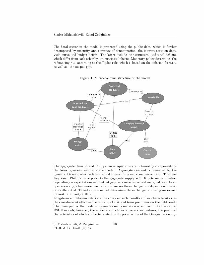
3 ModelThe fiscal forecasting and stress scenario analysis discussed in the following sectionsare based on the macro-fiscal model that is built using the approach developedby Kamenik et al. (2013). It is based on the new-Keynesian approach and takesthe non-Ricardian behavior of economic agents into consideration. Translating intomicrofoundations’ language the model structure represents households, intermediate-and final-goods producers, competitive financial markets, the foreign and fiscal sectorsand the central bank. The mechanism of their behavior is exhibited in the Figure 1.



The fiscal sector in the model is presented using the public debt, which is furtherdecomposed by maturity and currency of denomination, the interest costs on debt,yield curve and budget deficit. The latter includes the structural and total deficits,which differ from each other by automatic stabilizers. Monetary policy determines therefinancing rate according to the Taylor rule, which is based on the inflation forecast,as well as, the output gap.

Figure 1: Microeconomic structure of the model

The aggregate demand and Phillips curve equations are noteworthy components ofthe New-Keynesian nature of the model. Aggregate demand is presented by thedynamic IS curve, which relates the real interest rates and economic activity. The new-Keynesian Phillips curve presents the aggregate supply side. It determines inflationdepending on expectations and output gap, as a measure of real marginal cost. In anopen economy, a free movement of capital makes the exchange rate depend on interestrate differential. Therefore, the model determines the exchange rate using uncoveredinterest rate parity (UIP).Long-term equilibrium relationships consider such non-Ricardian characteristics asthe crowding-out effect and sensitivity of risk and term premiums on the debt level.The main part of the model’s microeconomic foundation is similar to the theoreticalDSGE models; however, the model also includes some ad-hoc features, the practicalcharacteristics of which are better suited to the peculiarities of the Georgian economy.


20


This provides the opportunity to increase the quality of forecasts. Therefore, due topractical reasons, we refrain from a lengthy discussion of the model’s microfoundationsand focus only on its reduced form and its applications.The main equations that are different from the original model by Kamenik et al.(2013) are discussed briefly in the following subsections.

3.1 Fiscal policyAccording to the model, fiscal policy determines 1) the structural deficit, which iscalculated using a specific rule, 2) debt-target, which is a given value of debt-to-GDPratio, and 3) decomposition of debt according to maturity and currency.The model is solved under the assumption of rational expectations among economicagents. Consequently, in order to ensure realistic results, it is important that thepublic’s trust in sustainability of debt around its target is high. Due to the factthat small and open economies are often significantly impacted by external shocksand market participant sentiments, it is not sufficient to merely meet the Maastrichtcriteria. In this case, in order to gain investor confidence, the level of debt-targetmust be significantly lower than the upper-bound of debt-to-GDP ratio given by theMaastricht treaty.In the model structural deficit is defined by the following equation:

sdt = αt (sdt−1 + f4yt) + (1− αt) sdtart + εsdt (6)

where sdt is the ratio of the (overall) structural deficit to GDP, yt is the output gap,f4 is a fiscal policy parameter, which defines the cyclicality of the fiscal rule, αt is apolicy preference parameter and εsdt is the discretionary shock of the structural deficit.sdtart defines the level of overall deficit, which is consistent with the debt target:

sdtart =(

1− 1 + εetµet

1 + nyet

)dtart (7)

nyet is the expected growth rate of the nominal GDP in the future time periods,εet – expected nominal exchange rate depreciation rate and µet – expected share offoreign debt, whereas dtart is the target debt-to-GDP level. On the other hand, debt-to-GDP accumulates according to the following law-of-motion:

dt = 1 + εtµt1 + nyt

dt−1 + odt (8)

where dt is the actual debt-to-GDP, odt – overall deficit-to-GDP and the rest arethe same as in the equation (7), but without e superscript, indicating actual valuesinstead of expected.One of the most important differences between our paper and Kamenik et al. (2013) isthe inclusion of terms εetµet and εtµt in the equations (7) and (8). These terms capture,



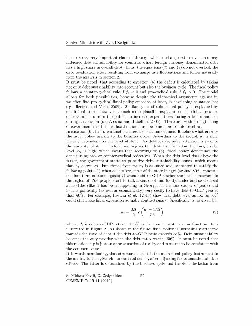
in our view, very important channel through which exchange rate movements mayinfluence debt-sustainability for countries where foreign currency denominated debthas a high share in overall debt. Thus, the equations (7) and (8) do not overlook thedebt revaluation effect resulting from exchange rate fluctuations and follow naturallyfrom the analysis in section 2.It must be noted, that according to equation (6) the deficit is calculated by takingnot only debt sustainability into account but also the business cycle. The fiscal policyfollows a counter-cyclical rule if f4 < 0 and pro-cyclical rule if f4 > 0. The modelallows for both possibilities, because despite the theoretical arguments against it,we often find pro-cyclical fiscal policy episodes, at least, in developing countries (seee.g. Ilzetzki and Vegh, 2008). Similar types of suboptimal policy is explained bycredit limitations, however a much more plausible explanation is political pressureon governments from the public, to increase expenditures during a boom and notduring a recession (see Alesina and Tabellini, 2005). Therefore, with strengtheningof government institutions, fiscal policy must become more counter-cyclical.In equation (6), the αt parameter carries a special importance. It defines what prioritythe fiscal policy assigns to the business cycle. According to the model, αt is non-linearly dependent on the level of debt. As debt grows, more attention is paid tothe stability of it. Therefore, as long as the debt level is below the target debtlevel, αt is high, which means that according to (6), fiscal policy determines thedeficit using pro- or counter-cyclical objectives. When the debt level rises above thetarget, the government starts to prioritize debt sustainability issues, which meansthat αt decreases. Functional form for αt is assumed and calibrated to satisfy thefollowing points: 1) when debt is low, most of the state budget (around 80%) concernsmedium-term economic goals; 2) when debt-to-GDP reaches the level somewhere inthe region of 35% people start to talk about debt and its dynamics and so do fiscalauthorities (like it has been happening in Georgia for the last couple of years) and3) it is politically (as well as economically) very costly to have debt-to-GDP greaterthan 60%. For example, Ilzetzki et al. (2013) show that debt level as low as 60%could still make fiscal expansion actually contractionary. Specifically, αt is given by:

αt = 0.82 e

(dt − 47.5

7.5

)(9)

where, dt is debt-to-GDP ratio and e (·) is the complementary error function. It isillustrated in Figure 2. As shown in the figure, fiscal policy is increasingly attentivetowards the issue of debt if the debt-to-GDP ratio exceeds 35%. Debt sustainabilitybecomes the only priority when the debt ratio reaches 60%. It must be noted thatthis relationship is just an approximation of reality and is meant to be consistent withthe common sense.It is worth mentioning, that structural deficit is the main fiscal policy instrument inthe model. It then gives rise to the total deficit, after adjusting for automatic stabilizereffects. The latter is determined by the business cycle and the debt deviation from


22


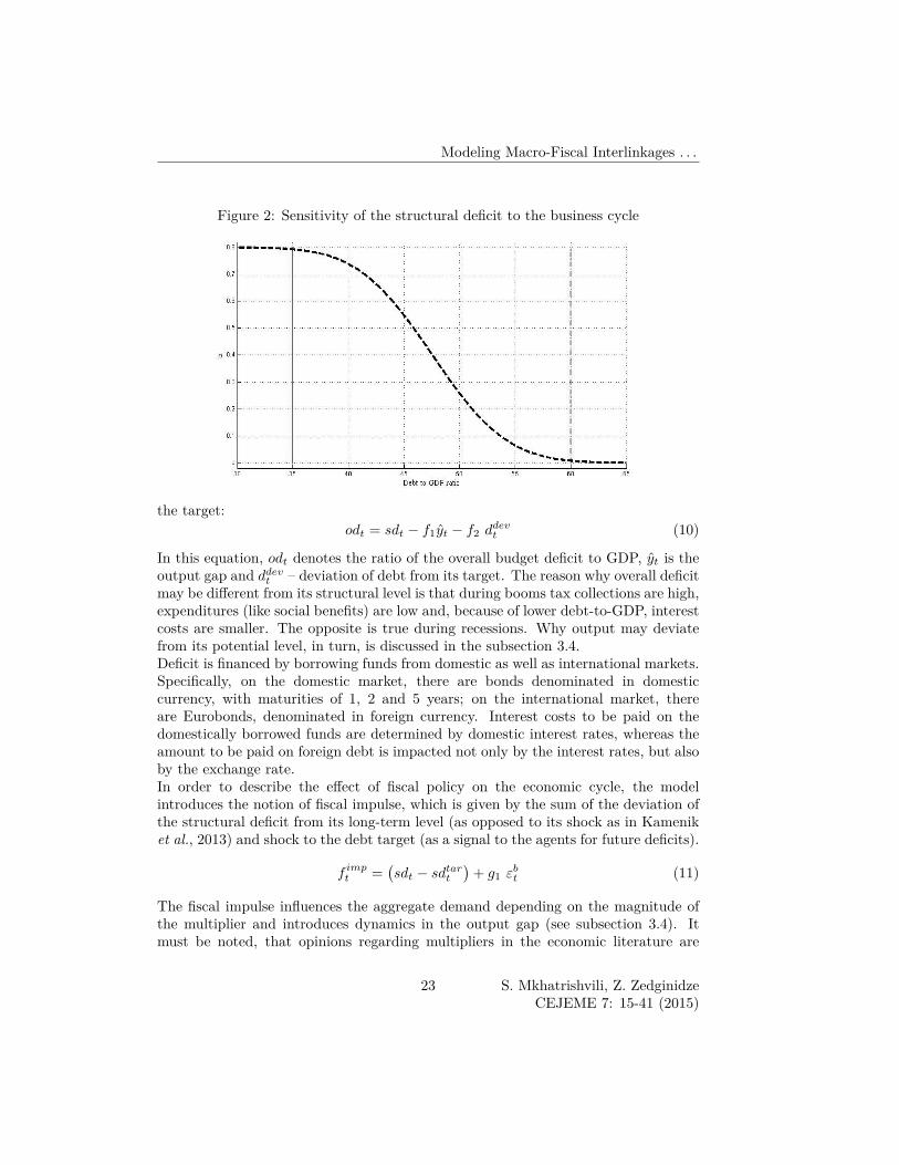
Figure 2: Sensitivity of the structural deficit to the business cycle

the target:odt = sdt − f1yt − f2 d

devt (10)

In this equation, odt denotes the ratio of the overall budget deficit to GDP, yt is theoutput gap and ddevt – deviation of debt from its target. The reason why overall deficitmay be different from its structural level is that during booms tax collections are high,expenditures (like social benefits) are low and, because of lower debt-to-GDP, interestcosts are smaller. The opposite is true during recessions. Why output may deviatefrom its potential level, in turn, is discussed in the subsection 3.4.Deficit is financed by borrowing funds from domestic as well as international markets.Specifically, on the domestic market, there are bonds denominated in domesticcurrency, with maturities of 1, 2 and 5 years; on the international market, thereare Eurobonds, denominated in foreign currency. Interest costs to be paid on thedomestically borrowed funds are determined by domestic interest rates, whereas theamount to be paid on foreign debt is impacted not only by the interest rates, but alsoby the exchange rate.In order to describe the effect of fiscal policy on the economic cycle, the modelintroduces the notion of fiscal impulse, which is given by the sum of the deviation ofthe structural deficit from its long-term level (as opposed to its shock as in Kameniket al., 2013) and shock to the debt target (as a signal to the agents for future deficits).

f impt =(sdt − sdtart

)+ g1 ε

bt (11)

The fiscal impulse influences the aggregate demand depending on the magnitude ofthe multiplier and introduces dynamics in the output gap (see subsection 3.4). Itmust be noted, that opinions regarding multipliers in the economic literature are



very heterogeneous. Its significance is highly dependent on the characteristics ofan economy, like the level of development and the size of the economy, as well as,the exchange rate regime and the level of debt. For example, Ilzetzki et al. (2013)document that long-run fiscal multipliers could be as low as -3 (for highly-indebtedcountries) and as high as 1.4 (in economies with fixed exchange rates). Additionally,the multiplier depends on the type of expenditure as government investments tendto have a higher multiplier than consumption. For example, Baxter and King (1993)show that public investment indeed has a very high multiplier. In the model, wedo not differentiate between the multipliers for investment or consumption, and theinterpretation of the value used here should be as an average figure consistent withthe structure of expenditures in Georgian economy throughout history.

3.2 Yield curveInterest rates, and generally, yield curves are one of the most important overlaps inmacroeconomic and fiscal policy. The model clearly defines the structure of debtmaturity. The interest rate on 1-year securities is i1t . It is the sum of the monetarypolicy rate and the time-varying spread. The 2-year interest rate i2t is determinedaccording to the current and expected 1-year interest rates, as well as, the termpremium (i.e. combining expectations hypothesis and liquidity premium theory):

i1t = it + spreadt (12)

i2t =i1t + Et

(i1t+1

)2 + tp2

t (13)

where, Et(i1t+1

)denotes the expected future 1-year interest rate, under rational

expectations based on information from the current period. tp2t is the term premium

for 2-year securities. The interest rate on 5-year securities is determined similarly.The interest rate on foreign securities is determined by risk premiums. Specifically,the interest rate on foreign debt is given by:

ifcyt = ift + pfcyt (14)

where ift is the foreign interest rate and pfcyt - a currency risk premium.The risk premium, in turn, depends on its long-term equilibrium value and deviationof debt from the level perceived by investors as stable.

3.3 Aggregate supplyOn the supply side, inflation is determined by the new-Keynesian Phillips curve. Forderiving it from microeconomic principles, one may start from profit maximizationproblem of the firms operating under monopolistic competition, taking such factors as


24


imported intermediate goods, price stickiness and indexation into account. Moreover,overall inflation includes domestic as well as imported prices:

πt = e1 Et (πt+1) + e2πimportt + (1− e1 − e2)πt−1 + e3yt + e4zt + επt + γπ,yε

yt (15)

Due to unit root in inflation, maintenance of it on its target is the result ofmonetary policy, which is achieved by satisfying the Taylor principle. Using importedintermediate goods in the production function introduces real exchange rate zt in thePhillips curve and in this regard the equation differs from the corresponding one inKamenik et al. (2013). Additionally, supply επt and technological progress εyt shocksalso affect inflation.

3.4 Aggregate demandIn the model, the demand side is presented by the dynamic IS curve, which relateseconomic activity and real interest rates. The relationship could be derived fromstandard microeconomic foundations. While Gali (2008) derives the basic dynamicIS equation, Gali and Monaccelli (2005) incorporate foreign economic activity andexchange rate in the equation and Smets and Wouters (2003) introduce sluggishness(i.e. lag) of demand in the equation. On top of that balance sheet effect, which maybe important if the economy is dollarized, and fiscal impulse are considered:

yt = k1Et (yt+1) + k2yt−1 − k3 (rt + pt) + k4zt + k5y∗t + k6f

impt + εyt + γy,gε

gt (16)

Thus, output depends on its expected future and past values, effective real interestrate rt, which combines domestic and foreign rates and risk premium pt, real exchangerate zt, foreign economic activity y∗

t and fiscal policy impulse f impt . On the shock side,there are demand εyt and expected economic activity εgt shocks. The latter describesthe wealth effect on current demand.It is worth emphasizing how we define potential output and, hence, output gap. Inthe literature to obtain output gap, usually it is either estimated with the Hodrick-Prescott filter (i.e. data is pre-filtered to exclude trends before going into structuralmodel) or it is defined as the difference between actual and potential output, wherethe latter is entirely model-implied (output level in no-frictions economy), which couldbe as volatile as the actual level itself, like in real business cycle frameworks. Ourapproach is to take somewhat balanced approach and we define potential output asfairly heavily depended on its past value but also determined by the long-term realinterest rates, as a proxy for crowding-out effect. It could also be hit by some shocks,like in times of crises, which change potential activity and have long-lasting effects.Finally, the equation for the potential output is fed into the Kalman filter along withthe rest of the structural equations. In this way potential level is estimated both as asmooth function of time, like in HP filter, and as a level consistent with the structureof the model economy, like in RBC literature. Therefore, actual output may deviatefrom its potential level because of short-term shocks, that affect actual values but not



potential, as well as long-term shocks, that first affect potential and only than actualactivity. Similar approach has been used by Cayen et al. (2009).In addition to the main equations discussed above, the model contains various otherequations, some of which are identities and some are other structural equations(e.g. imported inflation with the Balassa-Samuelson effect, Taylor rule for themonetary policy, UIP equations for nominal as well as real exchange rates). A partof the equations are exogenous by nature, but technically they are given by simpleautoregressive processes. This relates to the non-essential variables, which are not thefocus of the analysis and including them endogenously within the model will not haveany practical advantage. For the full list of these remaining equations see Kameniket al. (2013).

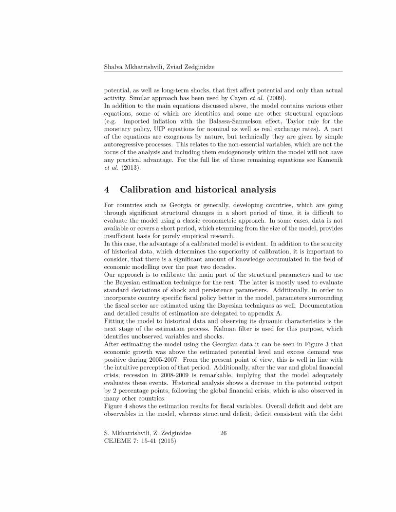
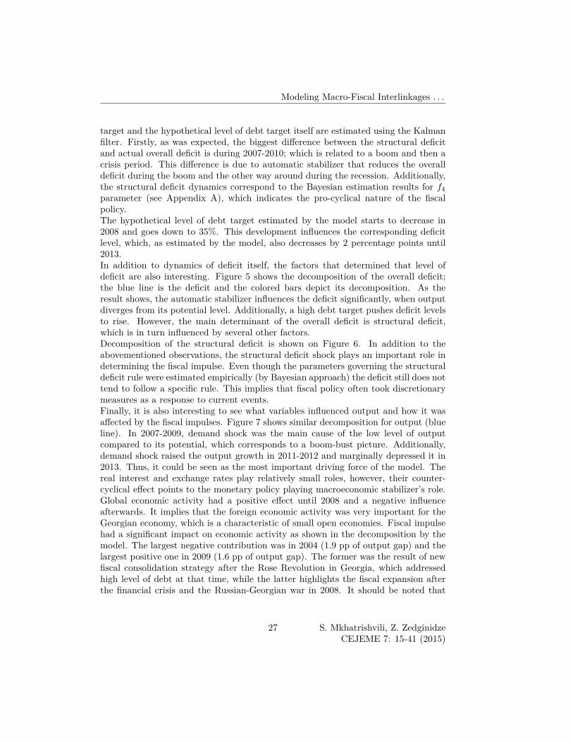
4 Calibration and historical analysisFor countries such as Georgia or generally, developing countries, which are goingthrough significant structural changes in a short period of time, it is difficult toevaluate the model using a classic econometric approach. In some cases, data is notavailable or covers a short period, which stemming from the size of the model, providesinsufficient basis for purely empirical research.In this case, the advantage of a calibrated model is evident. In addition to the scarcityof historical data, which determines the superiority of calibration, it is important toconsider, that there is a significant amount of knowledge accumulated in the field ofeconomic modelling over the past two decades.Our approach is to calibrate the main part of the structural parameters and to usethe Bayesian estimation technique for the rest. The latter is mostly used to evaluatestandard deviations of shock and persistence parameters. Additionally, in order toincorporate country specific fiscal policy better in the model, parameters surroundingthe fiscal sector are estimated using the Bayesian techniques as well. Documentationand detailed results of estimation are delegated to appendix A.Fitting the model to historical data and observing its dynamic characteristics is thenext stage of the estimation process. Kalman filter is used for this purpose, whichidentifies unobserved variables and shocks.After estimating the model using the Georgian data it can be seen in Figure 3 thateconomic growth was above the estimated potential level and excess demand waspositive during 2005-2007. From the present point of view, this is well in line withthe intuitive perception of that period. Additionally, after the war and global financialcrisis, recession in 2008-2009 is remarkable, implying that the model adequatelyevaluates these events. Historical analysis shows a decrease in the potential outputby 2 percentage points, following the global financial crisis, which is also observed inmany other countries.Figure 4 shows the estimation results for fiscal variables. Overall deficit and debt areobservables in the model, whereas structural deficit, deficit consistent with the debt


26


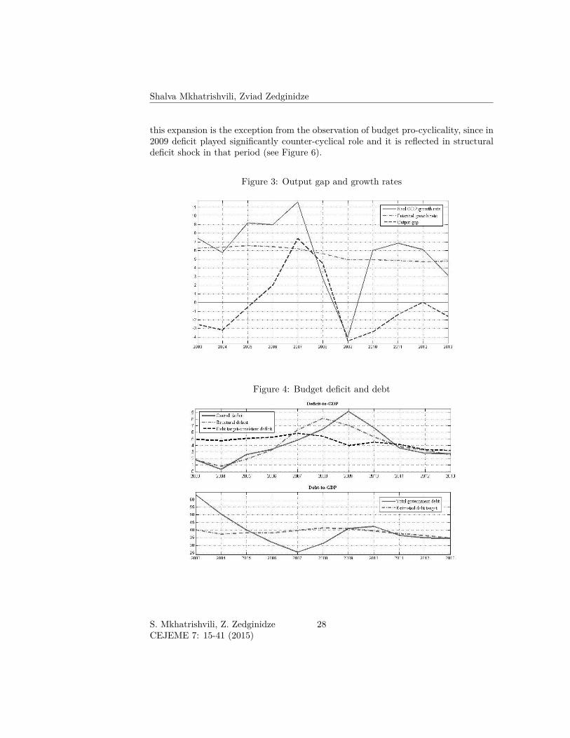
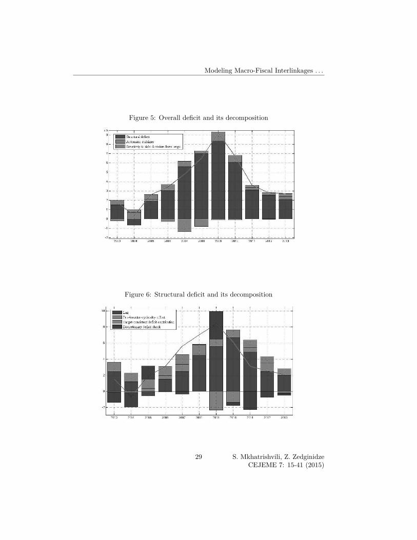
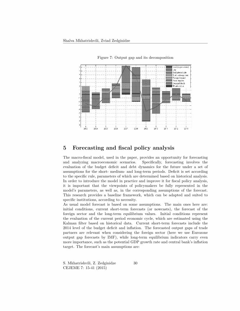
target and the hypothetical level of debt target itself are estimated using the Kalmanfilter. Firstly, as was expected, the biggest difference between the structural deficitand actual overall deficit is during 2007-2010; which is related to a boom and then acrisis period. This difference is due to automatic stabilizer that reduces the overalldeficit during the boom and the other way around during the recession. Additionally,the structural deficit dynamics correspond to the Bayesian estimation results for f4parameter (see Appendix A), which indicates the pro-cyclical nature of the fiscalpolicy.The hypothetical level of debt target estimated by the model starts to decrease in2008 and goes down to 35%. This development influences the corresponding deficitlevel, which, as estimated by the model, also decreases by 2 percentage points until2013.In addition to dynamics of deficit itself, the factors that determined that level ofdeficit are also interesting. Figure 5 shows the decomposition of the overall deficit;the blue line is the deficit and the colored bars depict its decomposition. As theresult shows, the automatic stabilizer influences the deficit significantly, when outputdiverges from its potential level. Additionally, a high debt target pushes deficit levelsto rise. However, the main determinant of the overall deficit is structural deficit,which is in turn influenced by several other factors.Decomposition of the structural deficit is shown on Figure 6. In addition to theabovementioned observations, the structural deficit shock plays an important role indetermining the fiscal impulse. Even though the parameters governing the structuraldeficit rule were estimated empirically (by Bayesian approach) the deficit still does nottend to follow a specific rule. This implies that fiscal policy often took discretionarymeasures as a response to current events.Finally, it is also interesting to see what variables influenced output and how it wasaffected by the fiscal impulses. Figure 7 shows similar decomposition for output (blueline). In 2007-2009, demand shock was the main cause of the low level of outputcompared to its potential, which corresponds to a boom-bust picture. Additionally,demand shock raised the output growth in 2011-2012 and marginally depressed it in2013. Thus, it could be seen as the most important driving force of the model. Thereal interest and exchange rates play relatively small roles, however, their counter-cyclical effect points to the monetary policy playing macroeconomic stabilizer’s role.Global economic activity had a positive effect until 2008 and a negative influenceafterwards. It implies that the foreign economic activity was very important for theGeorgian economy, which is a characteristic of small open economies. Fiscal impulsehad a significant impact on economic activity as shown in the decomposition by themodel. The largest negative contribution was in 2004 (1.9 pp of output gap) and thelargest positive one in 2009 (1.6 pp of output gap). The former was the result of newfiscal consolidation strategy after the Rose Revolution in Georgia, which addressedhigh level of debt at that time, while the latter highlights the fiscal expansion afterthe financial crisis and the Russian-Georgian war in 2008. It should be noted that



this expansion is the exception from the observation of budget pro-cyclicality, since in2009 deficit played significantly counter-cyclical role and it is reflected in structuraldeficit shock in that period (see Figure 6).

Figure 3: Output gap and growth rates

Figure 4: Budget deficit and debt


28


Figure 5: Overall deficit and its decomposition

Figure 6: Structural deficit and its decomposition



Figure 7: Output gap and its decomposition

5 Forecasting and fiscal policy analysisThe macro-fiscal model, used in the paper, provides an opportunity for forecastingand analyzing macroeconomic scenarios. Specifically, forecasting involves theevaluation of the budget deficit and debt dynamics for the future under a set ofassumptions for the short- medium- and long-term periods. Deficit is set accordingto the specific rule, parameters of which are determined based on historical analysis.In order to introduce the model in practice and improve it for fiscal policy analysis,it is important that the viewpoints of policymakers be fully represented in themodel’s parameters, as well as, in the corresponding assumptions of the forecast.This research provides a baseline framework, which can be adapted and suited tospecific institutions, according to necessity.As usual model forecast is based on some assumptions. The main ones here are:initial conditions, current short-term forecasts (or nowcasts), the forecast of theforeign sector and the long-term equilibrium values. Initial conditions representthe evaluation of the current period economic cycle, which are estimated using theKalman filter based on historical data. Current short-term forecasts include the2014 level of the budget deficit and inflation. The forecasted output gaps of tradepartners are relevant when considering the foreign sector (here we use Eurozoneoutput gap forecasts by IMF), while long-term equilibrium indicators carry evenmore importance, such as the potential GDP growth rate and central bank’s inflationtarget. The forecast’s main assumptions are:


30


1. Overall deficit-to-GDP in 2014 is 3.7%. This is in line (at the time of writing)with the planned budget deficit by the Georgian fiscal authority. Worth notingthat, since deficit is endogenous in the model, for fixing it to a particular valuethe following trick is used: the algorithm searches for the most likely valuesof shocks that will bring deficit-to-GDP to a given level (i.e. combination ofshocks that maximizes the log-likelihood subject to the deficit-to-GDP tune forthe year 2014).

2. Potential real GDP growth rate in the medium term is 5% and in the long-termit reduces to 4%, in line with convergence. Trend real exchange rate appreciationalso decreases from 3% to 1% as a result of convergence. These convergencesin steady state values are implemented in the model by applying the followingtrick: instead of treating steady states of potential growth and real exchangerate appreciation as parameters, they are modeled as random walks with smallstandard deviations for shocks. This means that whatever the starting valuesare for these processes, these values continue to be steady states until a one-timeshock hits them, which, then, permanently changes steady-states. For example,if we tell the Kalman filter to start with 5% steady state of potential growthand then apply a one-time shock of the magnitude of -1 to it in 10 years’ time, itwill reduce the potential growth to 4% after 10 years from the first period, butwill maintain 5% value until that time. Cayen et al. (2009) show that modelingtrend growth rates as random walks, clearly defining transitory and permanentshocks and, in general, estimating trends consistent with the model structurecan be more efficient than estimating them entirely independently.

3. Inflation target is 5% and in the long-term is gradually reduced to 3%. This isbased on the strategy of monetary policy developed by the Georgian monetaryauthority and published on their webpage. Technically, this is implemented inthe model like the previous assumptions.

4. Targeted debt-to-GDP ratio is 35%. This is in line with the “Strategy 2020”constructed by the Georgian government (available only in Georgian) referringto debt-to-GDP less than 40% as reasonable. Also, informal statements indicatethat the implicit debt-target of the government is somewhere 35%.

5. Foreign output in 2014-2015 is below the potential level by 2.2% and 1.4%,respectively, according to IMF forecasts (at the time of writing). After 2015 thegap closes gradually at an autoregressive coefficient of 0.5.

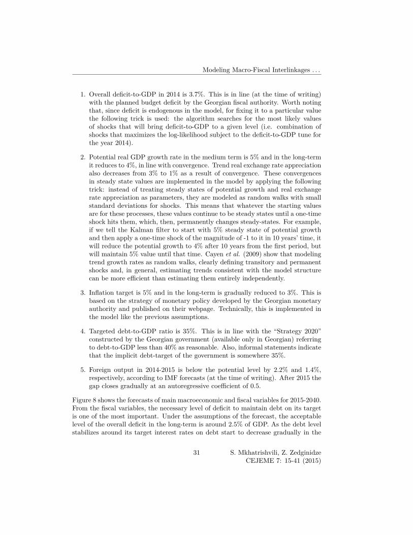
Figure 8 shows the forecasts of main macroeconomic and fiscal variables for 2015-2040.From the fiscal variables, the necessary level of deficit to maintain debt on its targetis one of the most important. Under the assumptions of the forecast, the acceptablelevel of the overall deficit in the long-term is around 2.5% of GDP. As the debt levelstabilizes around its target interest rates on debt start to decrease gradually in the



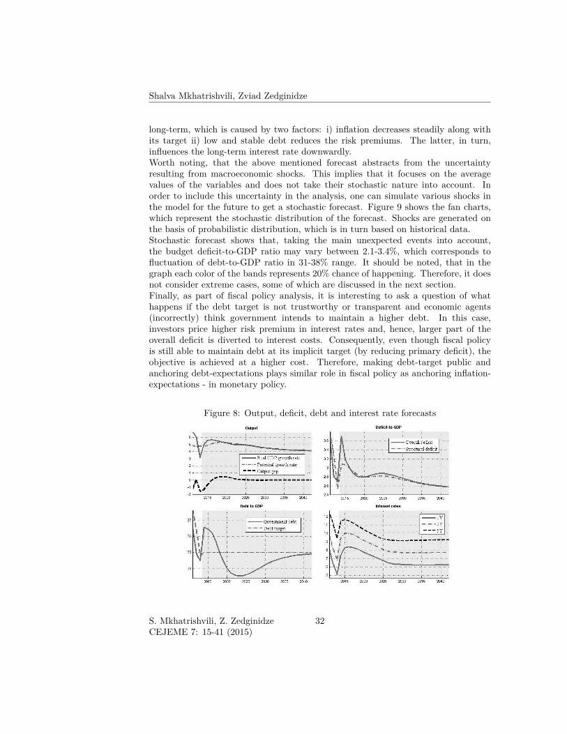
long-term, which is caused by two factors: i) inflation decreases steadily along withits target ii) low and stable debt reduces the risk premiums. The latter, in turn,influences the long-term interest rate downwardly.Worth noting, that the above mentioned forecast abstracts from the uncertaintyresulting from macroeconomic shocks. This implies that it focuses on the averagevalues of the variables and does not take their stochastic nature into account. Inorder to include this uncertainty in the analysis, one can simulate various shocks inthe model for the future to get a stochastic forecast. Figure 9 shows the fan charts,which represent the stochastic distribution of the forecast. Shocks are generated onthe basis of probabilistic distribution, which is in turn based on historical data.Stochastic forecast shows that, taking the main unexpected events into account,the budget deficit-to-GDP ratio may vary between 2.1-3.4%, which corresponds tofluctuation of debt-to-GDP ratio in 31-38% range. It should be noted, that in thegraph each color of the bands represents 20% chance of happening. Therefore, it doesnot consider extreme cases, some of which are discussed in the next section.Finally, as part of fiscal policy analysis, it is interesting to ask a question of whathappens if the debt target is not trustworthy or transparent and economic agents(incorrectly) think government intends to maintain a higher debt. In this case,investors price higher risk premium in interest rates and, hence, larger part of theoverall deficit is diverted to interest costs. Consequently, even though fiscal policyis still able to maintain debt at its implicit target (by reducing primary deficit), theobjective is achieved at a higher cost. Therefore, making debt-target public andanchoring debt-expectations plays similar role in fiscal policy as anchoring inflation-expectations - in monetary policy.

Figure 8: Output, deficit, debt and interest rate forecasts


32


Figure 9: Fan charts for deficit, debt, output and inflation

6 Stress scenario analysisIn addition to forecasts, the model gives an opportunity to study the influence ofmacroeconomic shocks on fiscal variables. This type of analysis is especially relevantfor debt sustainability analysis. Potential investors, as well as, policymakers maybenefit equally from evaluating the influence exogenous shocks may have on fiscalvariables and what the fiscal policy should look like, in order to minimize the negativeconsequences.The analysis uses hypothetical (and arbitrary) assumptions on external demand,country risk premium and exchange rate shocks. Specifically, stress scenarios are:

1. Reduction of the output growth rate in partner countries by 10 percentage points(demand shock). After the impact year growth rates in those countries revertback to normal at an autoregressive rate of 0.5, which means that the shockdies out in about 3 years.

2. Deterioration of a country’s (investment) risk premium by 10 percentage points(premium shock). The persistence of this shock is the same as in the demandshock scenario.

3. Depreciation of the currency by 25% (exchange rate shock). Unlike the previoustwo cases, this scenario is hit by a one-time nominal exchange rate depreciationshock.

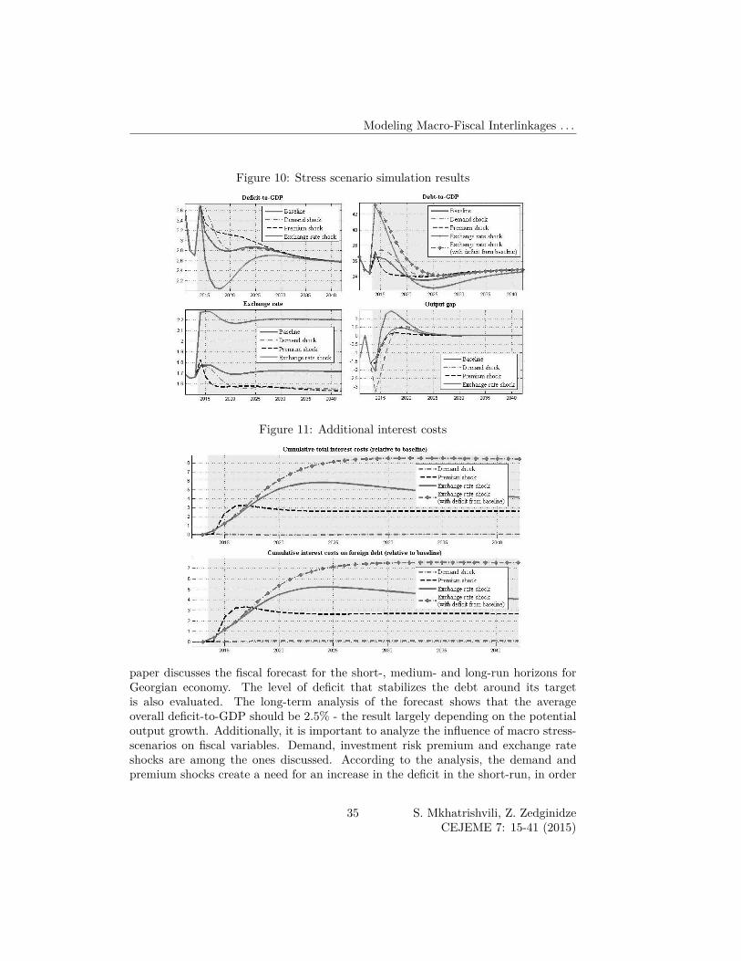
Figure 10 presents the results of the stress testing simulations for deficit, debt,exchange rate and output gap.Assuming that the model economy is a good approximation of reality implies that



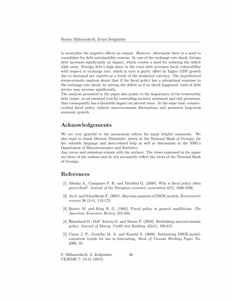
fiscal policy responses to different shocks suggested by the model are, by definition,optimal, given the objectives of fiscal authorities. Therefore, as the results show, thedemand and premium shocks lead to a temporary increase in deficit as part of theoptimal fiscal policy reaction, compared to the baseline scenario, which then createsa need for consolidation after the demand recovers. As a result the initially increaseddebt, which grew to 37-38%, returns to the target level in a few years. In the caseof such shocks, the negative output gap closes entirely by 2017. As for the exchangerate shock, in this case the optimal reaction of deficit is to maintain it at a lower levelthan the baseline scenario for a few years. There are two explanations for this: (I)because a large portion of the debt is denominated in foreign currency, depreciationof the domestic currency increases the debt-to-GDP ratio to 43% on impact and,consequently, there is a need for fiscal consolidation to ensure debt sustainability;(II) with a devaluation of the currency, there is an increase in foreign demand, whichinfluences the output gap positively and provides an opportunity to reduce the deficitmore painlessly. Finally, by combining the baseline and exchange rate scenarios, itcan be seen that even if fiscal policy does not reduce the deficit after the exchangerate shock (i.e. follows the path from the baseline scenario), the debt level still goesback to its target level. However, that takes an additional 4-5 years.As the analysis shows, despite the severe shocks, disciplined fiscal policy can fullycontrol the issue of debt sustainability. However, it must be noted, that defeatingthe shocks does not come without costs. Figure 11 shows the expenditures resultingfrom the above mentioned shocks, as measured by additional interest costs, relativeto GDP and compared to the baseline scenario, that are to be paid on debt.As can be seen, the largest cost comes from the exchange rate shock. Additionally,despite the fact that debt goes back to its target rate anyways, this type of shockcosts additional 4% of GDP spent on debt service, when fiscal policy is not conductedoptimally (i.e. when deficit follows the baseline path, even though exchange rate shockscenario was calling for tighter fiscal policy). Finally, during the demand shock, thereare no additional funds diverted to debt service, which is the result of eased monetarypolicy that reduces interest rates as a response to weak economic activity.

7 ConclusionsFiscal modelling is an important component of fiscal policy analysis. For thispurpose, the paper presents a new-Keynesian, DSGE approach-based, macro-fiscalmodel. Fiscal policy is endogenously presented in the model and its main instrument,the budget deficit, is set according to a certain rule. The approach takes intoaccount the dynamic and stochastic interrelationships between macro-fiscal variables.With the calibrated parameters, the model adequately interprets the historical data.In addition to calibration, Bayesian estimation technique is used, which providesadditional empirical ground for parameter values.In order to illustrate the applied features of the framework presented here, the


34


Figure 10: Stress scenario simulation results

Figure 11: Additional interest costs

paper discusses the fiscal forecast for the short-, medium- and long-run horizons forGeorgian economy. The level of deficit that stabilizes the debt around its targetis also evaluated. The long-term analysis of the forecast shows that the averageoverall deficit-to-GDP should be 2.5% - the result largely depending on the potentialoutput growth. Additionally, it is important to analyze the influence of macro stress-scenarios on fiscal variables. Demand, investment risk premium and exchange rateshocks are among the ones discussed. According to the analysis, the demand andpremium shocks create a need for an increase in the deficit in the short-run, in order



to neutralize the negative effects on output. However, afterwards there is a need toconsolidate for debt sustainability reasons. In case of the exchange rate shock, foreigndebt increases significantly on impact, which creates a need for reducing the deficitright away. Foreign debt’s high share in the total debt increases fiscal vulnerabilitywith respect to exchange rate, which in turn is partly offset by higher GDP growthdue to increased net exports as a result of the weakened currency. The hypotheticalstress-scenario analysis shows that if the fiscal policy has a suboptimal response tothe exchange rate shock, by setting the deficit as if no shock happened, costs of debtservice may increase significantly.The analysis presented in the paper also points to the importance of the trustworthydebt target, as an essential tool for controlling investor sentiment and risk premiums,that consequently has a favorable impact on interest rates. At the same time, counter-cyclical fiscal policy reduces macroeconomic fluctuations and promotes long-termeconomic growth.

AcknowledgementsWe are very grateful to the anonymous referee for many helpful comments. Wealso want to thank Mariam Tabatadze, intern at the National Bank of Georgia, forher valuable language and data-related help as well as discussants at the NBG’sDepartment of Macroeconomics and Statistics.Any errors and omissions remain with the authors. The views expressed in the paperare those of the authors and do not necessarily reflect the views of the National Bankof Georgia.

References[1] Alesina A., Campante F. R. and Tabellini G. (2008). Why is fiscal policy often

procyclical? Journal of the European economic association 6(5), 1006-1036.

[2] An S. and Schorfheide F. (2007). Bayesian analysis of DSGE models. Econometricreviews 26 (2-4), 113-172.

[3] Baxter M. and King R. G. (1993). Fiscal policy in general equilibrium. TheAmerican Economic Review, 315-334.

[4] Blanchard O., Dell’ Ariccia G. and Mauro P. (2010). Rethinking macroeconomicpolicy. Journal of Money, Credit and Banking, 42(s1), 199-215.

[5] Cayen J. P., Gosselin M. A. and Kozicki S. (2009). Estimating DSGE-model-consistent trends for use in forecasting. Bank of Canada Working Paper No.2009, 35.


36


[6] Coenen G. and Straub R. (2004). Non-Ricardian households and fiscal policy inan estimated DSGE model of the euro area. Manuscript, European Central Bank,2.

[7] Fernández-Villaverde J. and Rubio-Ramírez J. F. (2004). Estimating nonlineardynamic equilibrium economies: a likelihood approach. PIER Working PaperNo. 04-001.

[8] Fernández-Villaverde J. and Rubio-Ramírez J. F. (2005). Estimating dynamicequilibrium economies: linear versus nonlinear likelihood. Journal of AppliedEconometrics, 20(7), 891-910.

[9] Galí J. (2009). Monetary Policy, inflation, and the Business Cycle: Anintroduction to the new Keynesian Framework. Princeton University Press.

[10] Galí J., López-Salido J. D. and Vallés J. (2007). Understanding the effectsof government spending on consumption. Journal of the European EconomicAssociation, 5(1), 227-270.

[11] Galí J. and Monacelli T. (2005). Monetary policy and exchange rate volatility ina small open economy. The Review of Economic Studies, 72(3), 707-734.

[12] Garcia M. and Rigobon R. (2004). A risk management approach to emergingmarket’s sovereign debt sustainability with an application to Brazilian data.National Bureau of Economic Research (No. w10336).

[13] Guerrón-Quintana P. A. and Nason J. M. (2012). Bayesian estimation of DSGEmodels. Federal Reserve Bank of Philadelphia.

[14] Hubbard R. G. (1997). Capital-market imperfections and investment. NationalBureau of Economic Research (No. w5996).

[15] Konopczyński M. (2014). How Budget Deficit Impairs Long-Term Growth andWelfare under Perfect Capital Mobility. Central European Journal of EconomicModelling and Econometrics, 6(3), 129-152.

[16] Ilzetzki E., Mendoza E. G. and Végh C. A. (2013). How big (small?) are fiscalmultipliers? Journal of Monetary Economics, 60(2), 239-254.

[17] Ilzetzki E. and Végh C. A. (2008). Procyclical fiscal policy in developing countries:Truth or fiction?. National Bureau of Economic Research (No. w14191).

[18] International Monetary Fund (April 2014). World Economic Outlook (WEO).Available at: http://www.imf.org/external/pubs/ft/weo/2014/01/pdf/text.pdf


http://www.imf.org/external/pubs/ft/weo/2014/01/pdf/text.pdf

http://www.imf.org/external/pubs/ft/weo/2014/01/pdf/text.pdf


[19] Kamenik O., Tuma Z., Vavra D. and Smidova Z. (2013). A Simple Fiscal StressTesting Model: Case Studies of Austrian, Czech and German Economies, OECDEconomics Department Working Papers, No. 1074, OECD Publishing.

[20] Smets F., Wouters R. (2003). An estimated dynamic stochastic generalequilibrium model of the euro area. Journal of the European economicassociation, 1(5), 1123-1175.


38


A Bayesian Estimation ResultsIn the process of a Bayesian estimation, data is combined with the prior distribution,with the latter representing both economic theory and expert knowledge. As a result,we have a posterior distribution, the mode of which gives the point estimate of theparameter. Literature on Bayesian estimation has grown rapidly. For example,An and Schorfheide (2007) and Guerrón-Quintana and Nason (2012) provide verygood surveys of Bayesian estimation techniques for forward-looking economic models.Given this fact and that this paper uses Bayesian estimation only for a small subsetof model parameters, we do not discuss the estimation process into great details.Instead, we emphasize couple of important issues. First of all, Markov ChainMonte Carlo (MCMC) method is used to obtain an approximation to the exactposterior distribution, which is proportional to the product of data likelihood andprior distribution. More specifically:

f (θ|Y ) ∝ f (Y | θ)P (θ)

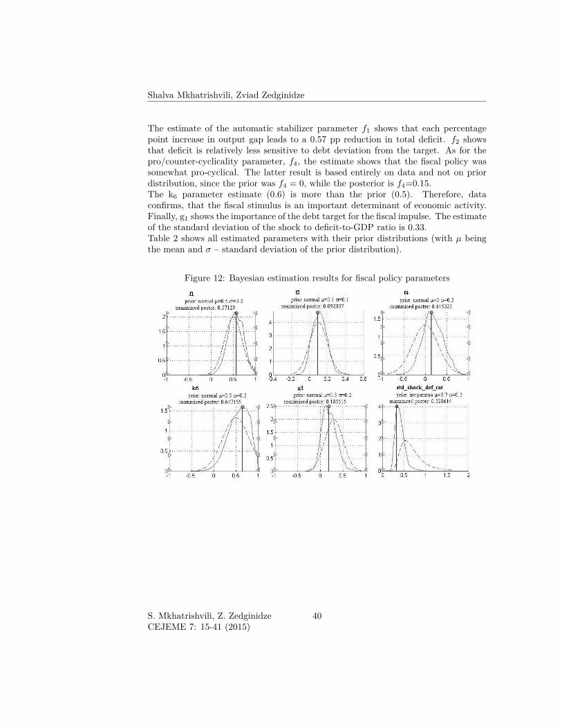
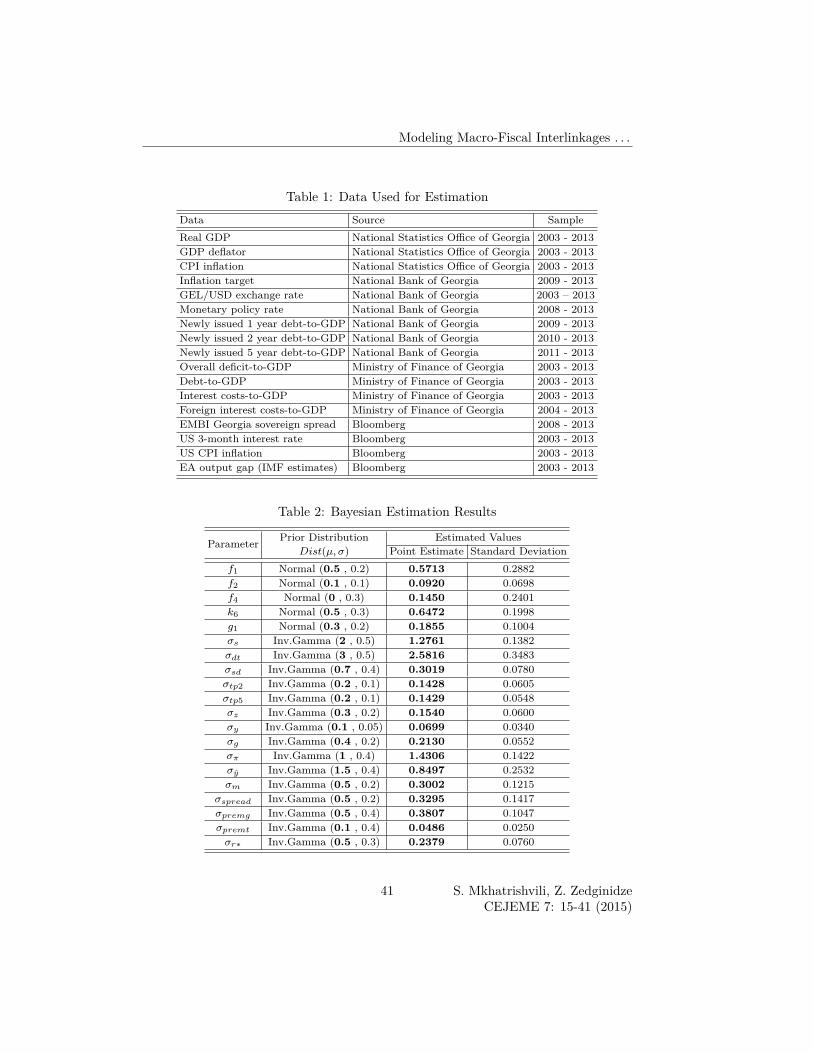
where f (θ|Y ) is the posterior distribution of the parameter vector θ, P (θ) is theprior distribution, specified by the modeler, and f (Y | θ) is the data likelihood forgiven parameter values. Secondly, data likelihood is obtained using Kalman filterwhere model equations are linearized and transformed into state-space representation.Thirdly, for a range of parameter values draws are made from the posteriordistribution, which enables us to maximize it with respect to parameter vectorand obtain final estimates. Finally, our approach indicates that we emphasize theimportance of non-linearities mainly when forecasting and simulating scenarios. Ifthe aim is to estimate parameters based on data that contain major non-linear events,like sovereign debt crisis, then non-linear filters have to be used. For example,Fernández-Villaverde and Rubio-Ramírez (2004) develop a Sequential Monte Carloalgorithm that delivers an estimate of the data likelihood in a non-linear model.Indeed, Fernández-Villaverde and Rubio-Ramírez (2005) show that this approach issuperior to standard Kalman filtering if the aim is to better suit the model to thedata. Fortunately, Georgian data does not contain the type of events when non-lineareffects would be especially active and, thus, our approach focuses on analyzing thesetypes of effects only for forecasting and stress-testing.As for the statistical data, Table 1 lists the series along with their sources and sampleperiods used for the estimation procedure. The data is yearly and fed into themodel without detrending, since the model estimates the trends with the rest ofthe structural equations (as described for GDP series in section 3.4).Figure 12 shows the results of estimating fiscal sector parameters using this approachfor f1, f2, f4, k6, g1 and the standard deviation of the deficit shock (however,technically the estimation is simultaneous for all parameters). The dashed blue lineshows the prior distribution, red line – posterior distribution and green – the pointestimate of the variable.



The estimate of the automatic stabilizer parameter f1 shows that each percentagepoint increase in output gap leads to a 0.57 pp reduction in total deficit. f2 showsthat deficit is relatively less sensitive to debt deviation from the target. As for thepro/counter-cyclicality parameter, f4, the estimate shows that the fiscal policy wassomewhat pro-cyclical. The latter result is based entirely on data and not on priordistribution, since the prior was f4 = 0, while the posterior is f4=0.15.The k6 parameter estimate (0.6) is more than the prior (0.5). Therefore, dataconfirms, that the fiscal stimulus is an important determinant of economic activity.Finally, g1 shows the importance of the debt target for the fiscal impulse. The estimateof the standard deviation of the shock to deficit-to-GDP ratio is 0.33.Table 2 shows all estimated parameters with their prior distributions (with µ beingthe mean and σ – standard deviation of the prior distribution).

Figure 12: Bayesian estimation results for fiscal policy parameters


40


Table 1: Data Used for EstimationData Source SampleReal GDP National Statistics Office of Georgia 2003 - 2013GDP deflator National Statistics Office of Georgia 2003 - 2013CPI inflation National Statistics Office of Georgia 2003 - 2013Inflation target National Bank of Georgia 2009 - 2013GEL/USD exchange rate National Bank of Georgia 2003 – 2013Monetary policy rate National Bank of Georgia 2008 - 2013Newly issued 1 year debt-to-GDP National Bank of Georgia 2009 - 2013Newly issued 2 year debt-to-GDP National Bank of Georgia 2010 - 2013Newly issued 5 year debt-to-GDP National Bank of Georgia 2011 - 2013Overall deficit-to-GDP Ministry of Finance of Georgia 2003 - 2013Debt-to-GDP Ministry of Finance of Georgia 2003 - 2013Interest costs-to-GDP Ministry of Finance of Georgia 2003 - 2013Foreign interest costs-to-GDP Ministry of Finance of Georgia 2004 - 2013EMBI Georgia sovereign spread Bloomberg 2008 - 2013US 3-month interest rate Bloomberg 2003 - 2013US CPI inflation Bloomberg 2003 - 2013EA output gap (IMF estimates) Bloomberg 2003 - 2013

Table 2: Bayesian Estimation Results

Parameter Prior Distribution Estimated ValuesDist(µ, σ) Point Estimate Standard Deviation

f1 Normal (0.5 , 0.2) 0.5713 0.2882f2 Normal (0.1 , 0.1) 0.0920 0.0698f4 Normal (0 , 0.3) 0.1450 0.2401k6 Normal (0.5 , 0.3) 0.6472 0.1998g1 Normal (0.3 , 0.2) 0.1855 0.1004σs Inv.Gamma (2 , 0.5) 1.2761 0.1382σdt Inv.Gamma (3 , 0.5) 2.5816 0.3483σsd Inv.Gamma (0.7 , 0.4) 0.3019 0.0780σtp2 Inv.Gamma (0.2 , 0.1) 0.1428 0.0605σtp5 Inv.Gamma (0.2 , 0.1) 0.1429 0.0548σz Inv.Gamma (0.3 , 0.2) 0.1540 0.0600σy Inv.Gamma (0.1 , 0.05) 0.0699 0.0340σg Inv.Gamma (0.4 , 0.2) 0.2130 0.0552σπ Inv.Gamma (1 , 0.4) 1.4306 0.1422σy Inv.Gamma (1.5 , 0.4) 0.8497 0.2532σm Inv.Gamma (0.5 , 0.2) 0.3002 0.1215

σspread Inv.Gamma (0.5 , 0.2) 0.3295 0.1417σpremg Inv.Gamma (0.5 , 0.4) 0.3807 0.1047σpremt Inv.Gamma (0.1 , 0.4) 0.0486 0.0250σr∗ Inv.Gamma (0.5 , 0.3) 0.2379 0.0760


Modeling Macro-Fiscal Interlinkages: Case of Georgia

Documents