Modeling lumber recovery in relation to selected tree characteristics in jack pine using sawing simulator Optitek

219Ann. For. Sci. 62 (2005) 219–228© INRA, EDP Sciences, 2005DOI: 10.1051/forest:2005013

Original article

Modeling lumber recovery in relation to selected tree characteristics in jack pine using sawing simulator Optitek

Shu-Yin ZHANG*, Que-Ju TONG

Forintek Canada Corp., 319 rue Franquet, Sainte-Foy, Québec, Canada G1P 4R4

(Received 26 May 2004; accepted 31 August 2004)

Abstract – End uses and product recovery are important considerations in forest management decision-making. This study intended to developgeneral tree-level lumber volume recovery models for jack pine. A sample of 154 jack pine trees collected from natural stands was scanned toobtain 3-D stem geometry for sawing simulation under two sawmill layouts, a stud mill and a random mill with optimized bucking, using sawingsimulator Optitek. Three model forms were chosen to describe the quantitative relationship between simulated lumber volume recovery andtree characteristics. It was found that lumber volume recovery of individual trees from both sawmills could be well estimated from DBH usinga second-order polynomial equation. Adding tree height into the model resulted in a small but significant improvement in the goodness of themodel. Adding tree taper into the model that already included DBH and tree height no longer improved the goodness significantly. The powerfunction form involving only DBH or both DBH and tree height as variables was also found to be suitable for the stud mill; exponential formswere least suitable. The second-order polynomial model with DBH alone was the most suitable model when inventory records DBH only, whilethe second-order polynomial model and the power model involving two variables (DBH and tree height) for the random mill and the stud mill,respectively, were better when both DBH and tree height are available.

tree characteristics / sawing simulation / Optitek / lumber recovery / general model

Résumé – Modélisation du rendement en sciages en relation avec certaines caractéristiques du pin baumier en utilisant le logiciel desimulation Optitek. L’utilisation finale et le rendement en produits sont des considérations importantes dans la prise de décision enaménagement forestier. Cette étude vise à développer des modèles généraux de rendement en volume au niveau de l’arbre du pin baumier. Unéchantillon de 154 arbres de sapin baumier récoltés dans des peuplements naturels a été scanné pour obtenir la géométrie 3-D des tiges poureffectuer la simulation selon deux configurations d’usine, soit une scierie de bois de colombage et une usine variable avec tronçonnage optimiséavec le simulateur de sciage Optitek. Trois formes de modèles ont été choisies pour décrire la relation quantitative entre le rendement en sciagesimulé et les caractéristiques de l’arbre. Il semble que le rendement en sciage d’arbres individuels provenant des deux scieries peut être bienestimé à partir du DHP en utilisant une équation polynomiale de deuxième ordre. L’ajout de la hauteur de l’arbre aux résultats du modèle estune petite amélioration, mais tout de même significative pour la validité du modèle. Toutefois, l’ajout du défilement de l’arbre à un modèleincluant déjà le DHP et la hauteur de l’arbre n’améliore pas significativement la validité. Les équations de fonction puissance impliquantseulement le DHP ou le DHP et la hauteur de l’arbre comme variables se sont avérées appropriées pour l’usine de colombage, alors que leséquations exponentielles l’étaient moins. Le modèle polynomial de deuxième ordre (modèle 2) avec DHP seulement est le modèle le plusapproprié lorsque l’inventaire enregistre seulement le DHP, alors que le modèle polynomial de second ordre et le modèle fonction puissanceimpliquant 2 variables (DHP et hauteur de l’arbre pour l’usine variable et l’usine de colombage, respectivement, sont meilleurs lorsque le DHPet la hauteur de l’arbre sont disponibles.

caractéristiques de l’arbre / simulation du sciage / Optitek / rendement en sciages / modèle général

1. INTRODUCTION

Forest management in eastern Canada has long been focusedon maximum stand yield (wood volume). It is known to bothforest managers and sawmills that each cubic meter of wooddoes not produce the same yield in terms of product recovery.

This means that a volume-oriented forest management strategydoes not necessarily lead to maximum product recovery andbest return, as several recent studies [22, 23] have reported. Asthe forest industry in eastern Canada has been moving towardboth intensive forest management and value-added products inrecent years, it is becoming important that end uses and product

* Corresponding author: [email protected]

Article published by EDP Sciences and available at http://www.edpsciences.org/forest or http://dx.doi.org/10.1051/forest:2005013

http://www.edpsciences.org/forest

http://dx.doi.org/10.1051/forest:2005013

220 S.-Y. Zhang, Q.-J. Tong

recovery be taken into consideration during forest managementdecision-making. To this end, it is necessary to develop tree-level models to predict product recovery based on tree charac-teristics collected for forest inventory.

It is well known that lumber recovery is closely related tosome tree characteristics [9, 13]. For decades, many studies [8,11, 14, 17–19, 25] have evaluated lumber recovery in relationto log characteristics such as log size, geometry and quality.Limited studies have assessed the effect of various treecharacteristics on lumber recovery, including lumber volume[13], grade yield [1, 5] and product value [3, 9, 21, 24]. Moststudies, however, were based on the product recovery from aspecific sawmill. As a result, the models developed were onlyapplicable to the specific layouts and conditions of the sawmillswhere the lumber conversions were carried out. The developmentof advanced sawing simulation packages in recent years (e.g.Optitek), however, has allowed researchers to define “standardsawmills” and thus simulate product recovery from thesestandard sawmills to develop general tree-level models.

The present study intended to develop general models topredict lumber recovery from individual trees using selectedtree characteristics that are easy to measure and are usuallycollected for forest inventory. Jack pine (Pinus banksianaLamb.), one of the most important commercial and reforestationspecies in Eastern Canada, was selected for this study. Thisspecies is highly valued for lumber and pulp production, andalso holds great potential for intensive silviculture [10].Optitek, a powerful sawing simulation package developed byForintek Canada Corp. [6], was used to simulate lumber recovery.The sawing simulator has been validated and has been usedintensively across Canada since 1994. It can be employed tosimulate various operations in a softwood conversion mill,from bucking to optimized log breakdown, curved sawing, andoptimized edging and trimming. Two state-of-the-art sawmills,a stud mill and an optimized random mill, were defined foreastern Canada to “process” the stems. A stud mill is a softwoodsawmill which saws 8 ft logs into studs, while a random mill(also called random length dimension mill) processes 8–16 ftlogs. Lumber recoveries from each type of sawmill in relationto key tree characteristics of diameter at breast height (DBH)and total tree height were examined to develop general tree-level lumber recovery models for jack pine. Based on thegeneral models, product recovery from jack pine trees andstands could be estimated from forest inventory data. Thus,forest management decisions could be made in the context ofproduct recovery to achieve specific objectives (e.g., maximum

product yield, quality and value). A better understanding of therelationship between tree characteristics and lumber volumerecovery will also help the sawmill industry to better plan forwood supply.

2. MATERIALS AND METHODS

2.1. Sample selection

A jack pine precommercial thinning (PCT) trial located at 47° 01’59’’ N, 65° 01’ 00’’ W on lower Miramichi, New Brunswick, Canadaprovided the sample trees for this study. The stands naturally regen-erated from a fire in 1941. In 1966, when the stands were 25-years old,PCT was carried out and plots of different thinning intensities (spac-ings) were established by the New Brunswick Department of NaturalResources and Energy. In 2001, sample trees were collected from plotsof 4 spacings (control, 4 × 4, 5 × 5, 7 × 7 ft). From each spacing,6 sample trees per DBH class were randomly selected to cover eachmerchantable DBH class at 2-cm intervals (e.g. 10, 12, 14, …). Treessmaller than 10 cm DBH class were not considered in this studybecause the minimum saw log diameter is 9 cm (able to produce a 2 by3 stud). There were, however, an insufficient number of trees availablein the largest DBH classes in each plot to reach the targeted 6 treesper DBH class. In total, 154 sample trees including 39 from the control,39 from 4 × 4, 40 from 5 × 5, and 36 from 7 × 7 spacing were collected.Table I presents the summary statistics for the 154 sample trees. Theaverage tree DBH (outside bark) of 16.4 cm indicates that trees col-lected for this study were quite small.

2.2. Tree measurements

For each sample tree, the following tree characteristics were meas-ured: outside bark DBH, total tree length, tree length up to a 7-cmdiameter top, crown width in two opposite directions (North-South andEast-West), crown length, clear log length, and diameters of the 5 larg-est branches on the trunk. Delimbed and debarked trees were scannedwith a portable scanner to collect stem geometric data (true stemshape) at intervals of 10 cm along the stem. Geometric data includedcoordinates of cross-sections in 3-D space and diameters at both X andY axes. The data were compatible with Optitek and were used forbucking and sawing simulations. The data were also used to determinestem taper, total stem volume and merchantable stem volume for eachstem.

2.3. Sawing simulation

Data from the 154 scanned sample trees served as input for theOptitek sawmill simulations. Optitek is a sawing simulator developedby Forintek to “saw” a “real” shape log in different sawmill layouts

Table I. Summary statistics of the 154 sample trees collected from a naturally regenerated jack pine precommercial thinning trial located inMiramichi, New Brunswick, Canada.

DBH*(cm)

Total height (m)

Length below live crown (m)

Taper (cm/m)

Stem volume up to 7 cm (m3)

Merchantable volume (m3)

Mean 16.4 15.3 10.1 1.0 0.1515 0.1367

S.D. 3.9 1.71 1.1 0.2 0.0808 0.0878

Max. 23.8 18.62 13.04 1.65 0.38117 0.37491

Min. 9.2 9.25 7.5 0.5 0.02879 0.00133

* Outside bark DBH.




Modeling lumber recovery 221

and product combinations. In this study, two state-of-the-art sawmills,a stud mill and an optimized random mill, were defined for easternCanada to separately “saw” the 154 sample trees. In the stud mill, thestems were first bucked into logs of 2.44 m (8 ft) in length, and thenlogs were sent to the mill to be “cut” into lumber with optimized lum-ber volume recovery. In the random mill, the stems were first optimallybucked, and the optimized bucking solution was treated as the inputof the sawmill where the logs were converted into lumber with thehighest volume recovery. Consequently, products from the stud millwere primarily 2.44 m (8 ft) long studs, while products from the ran-dom mill ranged from 1.22 to 4.88 m (4 to 16 ft) in length. Lumberdimensions and grades were defined in a grade file for both sawmills.

2.4. Simulation results

Following proper sawmill equipment configuration, log data loading,and definition of product dimensions and grades, the process programwas executed. Each tree was sawn into pre-defined product combina-tions. Then, Optitek generated a simulation report. In the report, prod-uct volume and value yields for each tree for both primary products (e.g.lumber) and by-products (e.g. chips) were given in the sections of vol-ume and value performances. Bucking solutions and product summa-ries were also listed. Table II summarizes the lumber recovery andvalue returns from the 154 sample trees.

2.5. Lumber conversion

Actual lumber conversion for the 154 sample trees was carried outat a modern stud sawmill that parallels the typical stud mill definedfor Optitek simulation. Each sample tree was bucked into 8-foot-longlogs. The logs were sawn at a much slower speed than usual so thateach piece of lumber and board from each log could be tracked. Lum-

ber volume recovered from each sample tree was used to validate themodels developed from the simulated sawing results.

3. MODEL DEVELOPMENT

To develop empirical models, it is necessary to select propervariables and model forms and to use good parameter estima-tion procedures and model validation techniques [7]. This studyassumed that lumber volume recovery from an individual treeis a function of tree size (DBH and tree height) and tree geom-etry (taper), namely:

(1)

where V represents lumber volume (fbm) from a tree, D denotesinside bark DBH (cm), H is total tree height (m), and T denotesstem taper (%) calculated based on tree height up to the 7-cmdiameter top.

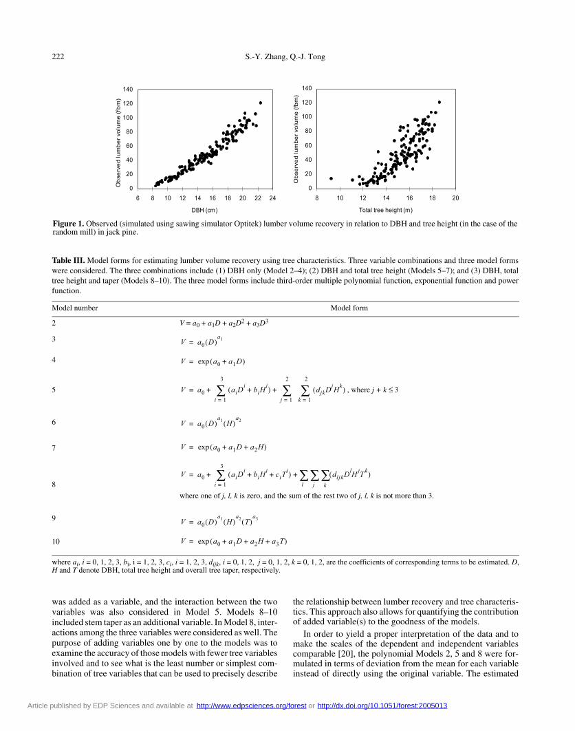
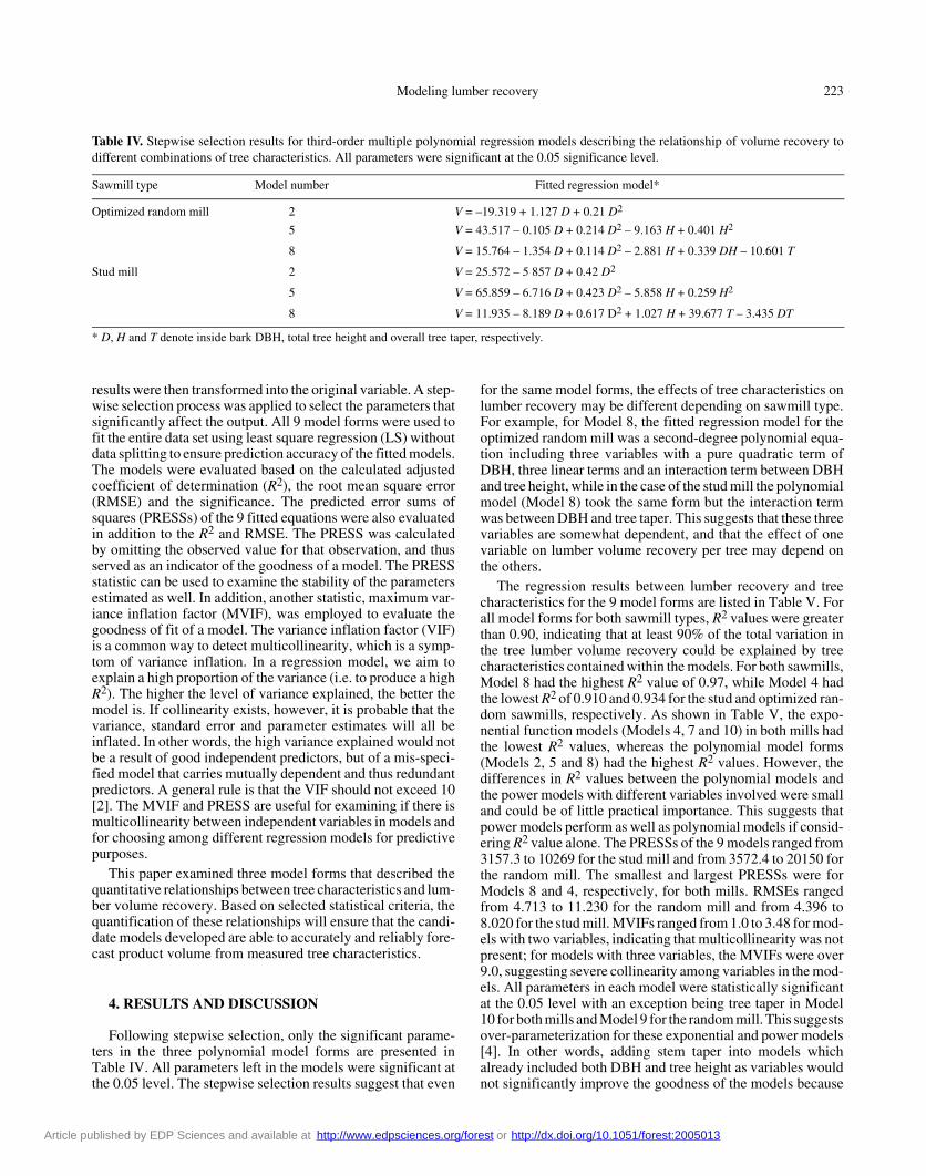
Equation (1) can be extended to many forms. The plots ofvolume recovery against both DBH and total tree height(Fig. 1) suggest a non-linear relationship between lumber vol-ume recovery and tree characteristics. This study consideredthree types of model forms: multiple polynomial function,exponential function and power function. Full third-order mod-els with one, two and three variables were chosen for multiplepolynomial models, respectively. Table III lists the differentmodel forms examined with different variables. Models 2–4considered the relationship of lumber volume recovery withDBH only, as many studies have reported that log diameter(DBH) contributes more to lumber volume recovery than otherparameters such as tree height [24]. In Models 5–7, tree height

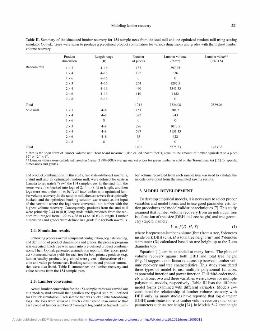
Table II. Summary of the simulated lumber recovery for 154 sample trees from the stud mill and the optimized random mill using sawingsimulator Optitek. Trees were sawn to produce a predefined product combination for various dimensions and grades with the highest lumbervolume recovery.

Product dimension

Length range(ft)

Number of pieces

Lumber volume(fbm*)

Lumber value** (CND $)

Random mill 1 × 3 4–16 187 397.25

1 × 4 4–16 192 636

1 × 6 8–16 0 0

2 × 3 4–16 264 1297.5

2 × 4 4–16 460 3543.33

2 × 6 4–16 110 1452

2 × 8 8–16 0 0

Total 1213 7326.08 2589.04

Stud mill 1 × 3 4–8 151 301.5

1 × 4 4–8 322 843

1 × 6 8 0 0

2 × 3 4–8 276 1077.5

2 × 4 4–8 597 3131.33

2 × 6 4–8 55 422

2 × 8 8 0 0

Total 1401 5775.33 1783.38

* fbm is the short form of lumber volume unit “foot board measure” (also called “board foot”), equal to the amount of timber equivalent to a piece12’’ × 12’’ × 1’’.** Lumber values were calculated based on 5-year (1998–2003) average market prices for green lumber as sold on the Toronto market [15] for specificdimensions and grades.

V f D, H, T( )=





was added as a variable, and the interaction between the twovariables was also considered in Model 5. Models 8–10included stem taper as an additional variable. In Model 8, inter-actions among the three variables were considered as well. Thepurpose of adding variables one by one to the models was toexamine the accuracy of those models with fewer tree variablesinvolved and to see what is the least number or simplest com-bination of tree variables that can be used to precisely describe

the relationship between lumber recovery and tree characteris-tics. This approach also allows for quantifying the contributionof added variable(s) to the goodness of the models.

In order to yield a proper interpretation of the data and tomake the scales of the dependent and independent variablescomparable [20], the polynomial Models 2, 5 and 8 were for-mulated in terms of deviation from the mean for each variableinstead of directly using the original variable. The estimated

Table III. Model forms for estimating lumber volume recovery using tree characteristics. Three variable combinations and three model formswere considered. The three combinations include (1) DBH only (Model 2–4); (2) DBH and total tree height (Models 5–7); and (3) DBH, totaltree height and taper (Models 8–10). The three model forms include third-order multiple polynomial function, exponential function and powerfunction.

Model number Model form

2 V = a0 + a1D + a2D2 + a3D3

3

4

5 , where j + k ≤ 3

6

7

8

where one of j, l, k is zero, and the sum of the rest two of j, l, k is not more than 3.

9

10

where ai, i = 0, 1, 2, 3, bi, i = 1, 2, 3, ci, i = 1, 2, 3, dijk, i = 0, 1, 2, j = 0, 1, 2, k = 0, 1, 2, are the coefficients of corresponding terms to be estimated. D,H and T denote DBH, total tree height and overall tree taper, respectively.

Figure 1. Observed (simulated using sawing simulator Optitek) lumber volume recovery in relation to DBH and tree height (in the case of therandom mill) in jack pine.

V a0 D( )a1=

V a0 a1D+( )exp=

V a0 aiDi biH

i+( ) djkD

jHk( )k 1=

2

∑j 1=

2

∑+i 1=

3

∑+=

V a0 D( )a1 H( )

a2=

V a0 a1D a2H+ +( )exp=

V a0 aiDi biH

i ciTi

+ +( ) j∑ dljkD

lH jTk( )k∑

l∑+

i 1=

3

∑+=

V a0 D( )a1 H( )

a2 T( )a3=

V a0 a1D a2H a3T+ + +( )exp=





results were then transformed into the original variable. A step-wise selection process was applied to select the parameters thatsignificantly affect the output. All 9 model forms were used tofit the entire data set using least square regression (LS) withoutdata splitting to ensure prediction accuracy of the fitted models.The models were evaluated based on the calculated adjustedcoefficient of determination (R2), the root mean square error(RMSE) and the significance. The predicted error sums ofsquares (PRESSs) of the 9 fitted equations were also evaluatedin addition to the R2 and RMSE. The PRESS was calculatedby omitting the observed value for that observation, and thusserved as an indicator of the goodness of a model. The PRESSstatistic can be used to examine the stability of the parametersestimated as well. In addition, another statistic, maximum var-iance inflation factor (MVIF), was employed to evaluate thegoodness of fit of a model. The variance inflation factor (VIF)is a common way to detect multicollinearity, which is a symp-tom of variance inflation. In a regression model, we aim toexplain a high proportion of the variance (i.e. to produce a highR2). The higher the level of variance explained, the better themodel is. If collinearity exists, however, it is probable that thevariance, standard error and parameter estimates will all beinflated. In other words, the high variance explained would notbe a result of good independent predictors, but of a mis-speci-fied model that carries mutually dependent and thus redundantpredictors. A general rule is that the VIF should not exceed 10[2]. The MVIF and PRESS are useful for examining if there ismulticollinearity between independent variables in models andfor choosing among different regression models for predictivepurposes.

This paper examined three model forms that described thequantitative relationships between tree characteristics and lum-ber volume recovery. Based on selected statistical criteria, thequantification of these relationships will ensure that the candi-date models developed are able to accurately and reliably fore-cast product volume from measured tree characteristics.

4. RESULTS AND DISCUSSION

Following stepwise selection, only the significant parame-ters in the three polynomial model forms are presented inTable IV. All parameters left in the models were significant atthe 0.05 level. The stepwise selection results suggest that even

for the same model forms, the effects of tree characteristics onlumber recovery may be different depending on sawmill type.For example, for Model 8, the fitted regression model for theoptimized random mill was a second-degree polynomial equa-tion including three variables with a pure quadratic term ofDBH, three linear terms and an interaction term between DBHand tree height, while in the case of the stud mill the polynomialmodel (Model 8) took the same form but the interaction termwas between DBH and tree taper. This suggests that these threevariables are somewhat dependent, and that the effect of onevariable on lumber volume recovery per tree may depend onthe others.

The regression results between lumber recovery and treecharacteristics for the 9 model forms are listed in Table V. Forall model forms for both sawmill types, R2 values were greaterthan 0.90, indicating that at least 90% of the total variation inthe tree lumber volume recovery could be explained by treecharacteristics contained within the models. For both sawmills,Model 8 had the highest R2 value of 0.97, while Model 4 hadthe lowest R2 of 0.910 and 0.934 for the stud and optimized ran-dom sawmills, respectively. As shown in Table V, the expo-nential function models (Models 4, 7 and 10) in both mills hadthe lowest R2 values, whereas the polynomial model forms(Models 2, 5 and 8) had the highest R2 values. However, thedifferences in R2 values between the polynomial models andthe power models with different variables involved were smalland could be of little practical importance. This suggests thatpower models perform as well as polynomial models if consid-ering R2 value alone. The PRESSs of the 9 models ranged from3157.3 to 10269 for the stud mill and from 3572.4 to 20150 forthe random mill. The smallest and largest PRESSs were forModels 8 and 4, respectively, for both mills. RMSEs rangedfrom 4.713 to 11.230 for the random mill and from 4.396 to8.020 for the stud mill. MVIFs ranged from 1.0 to 3.48 for mod-els with two variables, indicating that multicollinearity was notpresent; for models with three variables, the MVIFs were over9.0, suggesting severe collinearity among variables in the mod-els. All parameters in each model were statistically significantat the 0.05 level with an exception being tree taper in Model10 for both mills and Model 9 for the random mill. This suggestsover-parameterization for these exponential and power models[4]. In other words, adding stem taper into models whichalready included both DBH and tree height as variables wouldnot significantly improve the goodness of the models because

Table IV. Stepwise selection results for third-order multiple polynomial regression models describing the relationship of volume recovery todifferent combinations of tree characteristics. All parameters were significant at the 0.05 significance level.

Sawmill type Model number Fitted regression model*

Optimized random mill 2 V = –19.319 + 1.127 D + 0.21 D2

5 V = 43.517 – 0.105 D + 0.214 D2 – 9.163 H + 0.401 H2

8 V = 15.764 – 1.354 D + 0.114 D2 – 2.881 H + 0.339 DH – 10.601 T

Stud mill 2 V = 25.572 – 5 857 D + 0.42 D2

5 V = 65.859 – 6.716 D + 0.423 D2 – 5.858 H + 0.259 H2

8 V = 11.935 – 8.189 D + 0.617 D2 + 1.027 H + 39.677 T – 3.435 DT

* D, H and T denote inside bark DBH, total tree height and overall tree taper, respectively.





stem taper in jack pine has been reported to be very closelyrelated to DBH and tree height [16].

It must be noted that the developed models in this studyapply to jack pine trees of a DBH up to 24 cm. As shown inTables IV and V, the variables in either fitted polynomial orpower models were between second or fourth power. This sug-gests that the predicted lumber recovery using these modelsincrease dramatically with increasing tree size. Therefore, fur-ther research is needed to consider larger tree sizes. It shouldalso be noted that the models were developed based on the treediameter at exact breast height, namely, diameter at tree heightof 1.3 m from the ground. Therefore, any inaccurate DBH datamay result in inaccurate prediction of tree lumber volumerecovery.

4.1. Lumber recovery in relation to DBH

Diameter is the most commonly measured tree parameterbecause it is a very important tree characteristic and the easiestto measure. If a model is developed to accurately predict lumberrecovery using DBH only, product recovery could be estimatedbased on any DBH data inventory. Models 2–4 were the 3 forms

describing the relationship of lumber recovery with DBH forindividual trees. As shown in Table V, DBH alone was able toexplain 90.9–95.8% and 93.5–96.1% of the variation in lumbervolume recovery from the optimized random mill and stud mill,respectively.

4.1.1. Scenario 1 optimized random mill

As shown in Table V, the R2 value of the fitted second-degree polynomial model (Model 2) was as high as 0.958, whilethe power model (Model 3) and the exponential model(Model 4) had R2 values of 0.954 and 0.91, respectively. Thisindicates that the exponential model was less suitable fordescribing the relationship of interest. Moreover, the fittedexponential equation also had a much higher RMSE andPRESS than did Model 2. Model 3 performed better thanModel 4 in terms of R2, RMSE and PRESS. However, in spiteof having a R2 value similar to that of Model 2, Model 3 wasnot as good as Model 2 in terms of RMSE and PRESS. UsingR2 as a criterion for discriminating competitive models canbe very hazardous [12]. Besides criteria like R2 and PRESS,the plots of the predicted residuals should be examined as well.

Table V. Parameter estimates and statistical criteria for the 9 models using least square regression. Two types of sawmills were considered.Four criteria were used to evaluate models.

Type of sawmill

Model Parameters1 Criteria

a0 a1/b1/c1 2 a2/b2 a3/d1 R2 RMSE PRESS MVIF

Opt

imiz

ed r

ando

m m

ill

2 –19.319 1.127 0.21 0.958 5.592 4937.7 1.0

3 0.019 (0.00**)3) 2.851 (0.00**) 0.954 7.183 8079.1 1.0

4 0.721 (0.00**) 0.195 (0.00**) 0.910 11.230 20150 1.0

5 43.517 –0.105/–9.163 0.214/0.401 0.967 4.773 3645.8 3.48

6 0.003 (0.00**) 2.467 (0.00**) 0.998 (0.00**) 0.962 6.235 6123.1 3.14

7 –0.253 (0.1308) 0.154 (0.00**) 0.103 (0.00**) 0.929 9.943 15861 3.06

8 15.764 –1.354/–2.881/–10.601 0.114/0 0/0.339 (DH) 0.970 4.713 3572.4 11.05

9 0.003 (0.00**) 2.637 (0.00**) 0.880 (0.00**) –0.146 (0.182) 0.962 6.244 6145.4 10.79

10 –0.319 (0.101) 0.147 (0.00**) 0.109 (0.00**) 0.103 (0.502) 0.928 9.870 15646 9.93

Stu

d m

ill

2 25.572 –5.857 0.42 0.961 4.988 3978.6 1.0

3 0.006 (0.00**) 3.170 (0.00**) 0.960 5.049 3985.9 1.0

4 0.069 (0.347) 0.219 (0.00**) 0.934 8.020 10269 1.0

5 65.859 –6.716/–5.858 0.4233/0.259 0.967 4.614 3247.4 3.48

6 0.002 (0.00**) 2.855 (0.00**) 0.817 (0.00**) 0.964 4.687 3445.8 3.14

7 –0.761 (0.00**) 0.184 (0.00**) 0.088 (0.00**) 0.944 7.392 8746.1 3.06

8 11.935 –8.189/1.027/39.677 0.617/0 0/–3.435 (DT) 0.970 4.396 3157.3 11.05

9 0.001 (0.00**) 3.126 (0.00**) 0.629 (0.00**) –0.232 (0.047*) 0.965 4.529 3219.8 10.79

10 –0.753 (0.00**) 0.185 (0.00**) 0.087 (0.00**) –0.012 (0.934) 0.944 7.424 8829.5 9.92

1 Estimated polynomial model forms 2, 5 and 8 for both random mill and stud mill are presented in Table IV. 2 Slashes between values for Models 5 and 8 separate coefficients for the same order variables. 3 Figures in parentheses represent probability levels (* denotes significance at p < 0.05 and ** denotes significance at p < 0.01). Letters in parenthesesrepresent variables. The coefficient of these variables are presented to the right. For example, the coefficient for variable (DH) in Model 8 for the opti-mized random mill was 0.339. All parameters for Models 2, 5 and 8 were significant at p < 0.05.





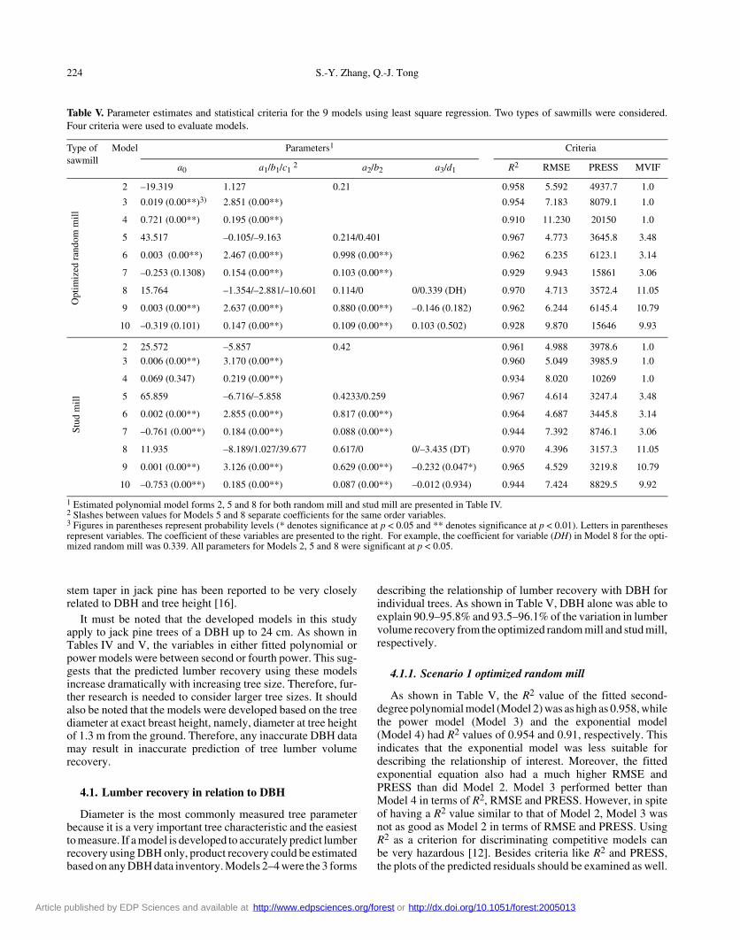
Figure 2 illustrates the predicted residuals against the fittedlumber recovery for the random mill for Models 2 and 3.Model 2 had a more evenly distributed residual plot over thefitted lumber volume than did Model 3. The residuals wereevenly and symmetrically spread on both sides of the zero linefor Model 2, while Model 3 showed a systematic residual dis-tribution pattern to some extent. Therefore, Model 2 was themost reliable in predicting lumber recovery from the optimizedrandom mill when only DBH was considered as a variable. Thepredicted residual plot for Model 2 appeared to have a widerresidual range in the right side than in the left side. Figure 1presents the plots of the measured DBH and tree height againstthe observed lumber volume recovery form the random mill.Lumber volume recoveries from trees of small DBH classesvaried within a relatively narrow range, while the volumerecoveries from trees of large DBH classes were scattered in awider range. A similar trend was noticed for lumber volumerecovery against tree height. This indicates that lumber volumerecovery from a larger tree was more variable than from asmaller tree. As a result, predicting lumber recovery for largertrees tended to be less accurate.

4.1.2. Scenario 2 stud mill

In the case of the stud mill, Model 2 also had the highestR2 value, followed by Model 3, whereas Model 4 had the lowest

R2 value (Tab. V). However, the difference in R2 values betweenModels 2 and 3 was very small and was likely inconsequential,particularly because differences in RMSE and PRESS betweenModels 2 and 3 were also very small. The predicted residualplots (Fig. 3) against the fitted lumber recovery also illustratedthat Models 2 and 3 had almost identical residual distributionpatterns and that the residuals were evenly distributed over therange of fitted lumber volumes. Despite having a R2 value ofas high as 0.93, Model 4 had much higher RMSE and PRESScompared to Models 2 and 3 (Tab. V), suggesting less accurateprediction by the exponential model. Therefore, statisticallyModels 2 and 3 were both adequate in estimating jack pine lum-ber volume recovery from the stud mill using DBH only.

4.2. Lumber recovery in relation to DBH and tree height

Tree height is another important tree characteristic affectinglumber recovery. It depends on site index and is often recordedfor forest inventory, although not as easily as DBH. Models 5–7in Tables IV and V described lumber volume recovery in rela-tion to both DBH and tree height.

4.2.1. Scenario 1 Optimized random mill

The estimated polynomial equation (Model 5) with the twovariables of DBH and total tree height is presented in Table IV.

Figure 2. Plots of residuals against fitted lumber volume recovery in the case of the random mill in jack pine. (a) Model 2 (second-order poly-nomial model with one variable “DBH”); (b) Model 3 (power model with one variable “DBH”).

Figure 3. Plots of residuals against fitted lumber volume recovery in the case of the stud mill in jack pine. (a) Model 2 (second-order polynomialmodel with one variable “DBH”); (b) Model 3 (power model with one variable “DBH”).





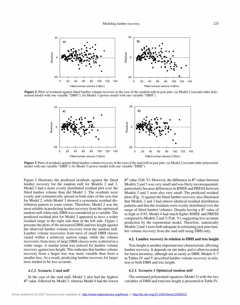
Estimated parameters for the pure quadratic terms of DBH andtree height were highly significant, while the parameters for thethird order terms and for the cross product of DBH and treeheight were not statistically significant at the 0.05 level. Thisimplies that tree height and DBH both have a quadratic effecton lumber volume recovery from the random mill. Model 5 hada R2 value of 0.97, higher than those of both Models 6 and 7,and its RMSE and PRESS were considerably lower. The expo-nential model (Model 7) may not be considered appropriate dueto its prominent RMSE and PRESS even though its R2 valuewas high at 0.929. Similarly to Model 3 for the random mill,the power model (Model 6) had a fairly comparable R2 valueand appreciably higher RMSE and PRESS than the polynomialmodel (Model 5), indicating less suitability as a predictor. Asshown in Figure 4, the plot of residuals against fitted lumbervolume recovery for Model 5 showed that the residuals wererandomly scattered on both sides of the zero line. Therefore,Model 5 was adequate for predicting jack pine lumber volumerecovery from the random mill using DBH and total tree height.

4.2.2. Scenario 2 stud mill

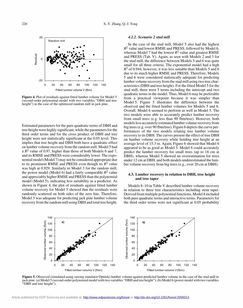
In the case of the stud mill, Model 5 also had the highestR2 value and lowest RMSE and PRESS, followed by Model 6,whereas Model 7 had the lowest R2 value and greatest RMSEand PRESS (Tab. V). Again, as seen with Models 2 and 3 forthe stud mill, the difference between Models 5 and 6 was quitesmall for all three criteria. The exponential model had a highR2 of 0.944, however, it was less suitable than Models 5 and 6due to its much higher RMSE and PRESS. Therefore, Models5 and 6 were considered statistically adequate for predictinglumber volume recovery from the stud mill using two tree char-acteristics (DBH and tree height). For the fitted Model 5 for thestud mill, there were 5 terms including the intercept and twoquadratic terms in the model. Thus, Model 6 may be preferablefrom a practical viewpoint because it was simpler thanModel 5. Figure 5 illustrates the difference between theobserved and the fitted lumber volumes for Models 5 and 6.Overall, Model 6 seemed to perform as well as Model 5. Thetwo models were able to accurately predict lumber recoveryfrom small trees (e.g. less than 90 fbm/tree). However, bothmodels less accurately estimated lumber volume recovery frombig trees (e.g. over 90 fbm/tree). Figure 6 depicts the curve per-formances of the two models relating tree lumber volumerecovery to its DBH. The curves present the effect of tree DBHon lumber volume recovery while holding tree height at anaverage level of 15.3 m. Again, Figure 6 showed that Model 6appeared to be as good as Model 5. Model 6 could accuratelypredict the lumber recovery for small trees (up to 18 cm atDBH), whereas Model 5 showed an overestimation for treesunder 12 cm at DBH, and both models underestimated the lum-ber volume recovery from big trees (e.g., over 20 cm at DBH).

4.3. Lumber recovery in relation to DBH, tree height and tree taper

Models 8–10 in Table V described lumber volume recoveryin relation to three tree characteristics including stem taper.Derived from multiple polynomial functions, Model 8 includedboth pure quadratic terms and interactive terms. Parameters forthe third order terms were not significant at 0.05 probability

Figure 4. Plot of residuals against fitted lumber volume for Model 5(second-order polynomial model with two variables “DBH and treeheight”) in the case of the optimized random mill in jack pine.

Figure 5. Observed (simulated using sawing simulator Optitek) lumber volume against predicted lumber volume in the case of the stud mill injack pine. (a) Model 5 (second-order polynomial model with two variables “DBH and tree height”); (b) Model 6 (power model with two variables“DBH and tree height”).





level following stepwise selection for both mills; for the ran-dom mill, the effect of tree DBH on lumber volume recoverywas dependent on the total tree height, while for the stud millthe DBH effect depended on tree taper, and vice versa. Com-pared with Model 5, Model 8 (including the additional variableof tree taper) did not seem to provide an appreciable improve-ment in either R2 value or RMSE and PRESS. In contrast, withthe additional variable tree taper, the MVIF increased from 3.48to 11.05 for both mills, which implies the presence of severemulticollinearity among the three variables in Model 8. A sim-ilar trend was observed in Model 9 for the stud mill. It thereforemade sense to omit the variable tree taper from the model spec-ification even though the variable appeared statistically signif-icant. On the other hand, the significance levels of the param-eters estimated for tree taper in Models 9 and 10 were 0.182and 0.502, respectively, in the case of the random mill, and0.047 and 0.934, respectively, in the case of the stud mill. Thisindicates that, statistically, tree taper should be excluded fromthe models as its impact on lumber volume recovery was notsignificant except for Model 9 for the stud mill, where tree tapercould be omitted due to the high variation inflation as statedabove. This seemed to be inconsistent with the common senseviewpoint that stem taper has a negative impact on tree productrecovery. It is well known that tree taper depends on DBH andtree height. As a matter of fact, a taper equation developed bySharma and Zhang [16] for jack pine using only DBH and totaltree height is able to accurately estimate diameter profile,explaining over 95% of the variation. Therefore, it was not sur-prising that adding tree taper to Models 9 and 10, which already

included both DBH and tree height, would not significantlyimprove the goodness of fit of the models. Overall, the threemodel forms with three variables including tree taper did notseem suitable for predicting the lumber volume recovery fromthe both sawmills.

4.4. Model validation

As discussed above, Models 2 and 5 for the random mill andModels 2, 3, 5 and 6 for the stud mill were considered to betterdescribe lumber volume recovery in relation to the selected treecharacteristics. Actual lumber volume recovery data of the154 sample trees sawn in a real stud sawmill were used to fur-ther validate the 4 models for the stud mill. The summary sta-tistics and paired T-test results for means for sawmill data andpredicted data using the 4 models are presented in Table VI.The significance levels (p values) for the differences betweenlumber volume recoveries from the real stud sawmill and fromthe 4 models were 0.554, 0.554, 0.591 and 0.537 for Model 2,3, 5 and 6, respectively. This suggests that there are no statis-tically significant differences between the predicted lumbervolume recovery and the actual volume recovery from the realstud sawmill, thus all 4 models are able to accurately predictlumber volume recovery. It appeared that all 4 models some-what overestimated the real lumber recovery from the largesttrees. This may happen as the largest trees usually come fromwider spacings where more jack pine trees contain severe stemdeformations. Overall, all 4 models slightly under-predictedlumber volume recovery. This might be due to the fact that the

Table VI. ANOVA analysis results for testing the fitness of candidate models for the stud mill using data from a real stud sawmill.

Max. (fbm) Min. (fbm) Mean (fbm) StDev T Stat. p value

Sawmill 99.58 3 38.77 22.18

Model 2 105.34 6.22 37.707 24.71 0.5933 0.5539

Model 3 108.88 6.39 37.701 24.79 0.6240 0.5536

Model 5 112.26 5.35 37.703 25.65 0.5383 0.5911

Model 6 115.66 5.29 37.671 25.43 0.6192 0.5367

Figure 6. Predicted lumber volume recovery of jack pine for the stud mill in relation to DBH while holding tree height at an average level of15.3 m. (a) Model 5 (second-order polynomial model with two variables “DBH and tree height”); (b) Model 6 (power model with two variables“DBH and tree height”).





actual size of green lumber produced in the real stud sawmillwas slightly smaller than that configured for the stud sawmillin the sawing simulator Optitek.

5. CONCLUSION

Using statistical methods, three model forms and their exten-sions with different variables involved in two types of sawmillswere studied for their ability to predict lumber volume recoveryfrom basic tree characteristics. The results demonstrated thatthe polynomial function form was the most suitable for predict-ing lumber volume recovery from the random mill, followedby the power function, while for the stud mill the power andpolynomial function forms were both good for describing lum-ber volume recovery from tree characteristics. The results alsoindicate that the exponential functions were the least suitable.For both sawmills, a second-order polynomial function withone variable, DBH, was able to explain as much as 95.83% ofthe total variation for the optimized random mill and 96.1% forthe stud mill. Adding tree height to the model led to a small butsignificant increase in the percentage of the variation explained.The power function form for the stud mill performed as wellas the polynomial function form. The power function may bepreferable for predicting lumber volume recovery from the studmill using DBH and tree height, as it was simpler. The studyalso indicates that adding tree taper to a model including DBHand tree height did not improve the goodness of fit of the modelas tree taper in jack pine can be well described by DBH and totaltree height. The second-order polynomial model (Model 2)with DBH alone could be used to accurately predict lumber vol-ume recovery from both stud and random mills when inventoryrecords DBH only, while the second-order polynomial model(Model 5) and the power model (Model 6) involving two var-iables (DBH and tree height) were better for the random milland the stud mill, respectively, when both DBH and tree heightare recorded for forest inventory.

REFERENCES

[1] Beauregard R.L., Gazo R., Ball R.D., Grade recovery, value, andreturn-to-log for the production of NZ visual grades (cuttings andframing) and Australian machine stress grades, Wood Fiber Sci. 34(2002) 485–502.

[2] Belsley D.A., Kuh E., Welsch R.E., Regression Diagnostics, JohnWiley and Sons, New York, NY, 1980.

[3] Briggs D.G., Tree value system: description and assumptions,General Technical Report Pacific Northwest Research Station,USDA Forest Service, No. PNW-GTR-239, 1989, 24 p.

[4] Draper N.R., Smith H., Applied regression analysis, 2nd ed., JohnWiley and Sons, New York, 1981.

[5] Fahey T.D., Grading second-growth Douglas-fir by basic treemeasurements, J. For. 4 (1980) 206–206.

[6] Forintek Canada Corp., Optitek: User’s guide, Forintek CanadaCorp., Sainte-Foy, Quebec, 1994, 185 p.

[7] Gujarati D.N., Basic econometrics, 3rd ed., McGraw-Hill, NewYork, 1995.

[8] Harless T.E.G., Wagner F.G., Steele P.H., Taylor F.W., YadamaV., McMillin C.W., Methodology for locating defects within hard-wood logs and determining their impacts on lumber-value yield,For. Prod. J. 41 (1991) 25–30.

[9] Kellogg R.M., Warren W.G., Evaluating western hemlock stemcharacteristics in terms of lumber value, Wood Fiber Sci. 16 (1984)583–597.

[10] Law K.N., Valade J.L., Status of the utilization of jack pine (Pinusbanksiana) in the pulp and paper industry, Can. J. For. Res. 24(1994) 2078–2084.

[11] Middleton G.R., Munro B.D., Log and lumber yields, in: KelloggR.M. (Ed.), Second-growth Douglas-fir: its management and con-version value, Special Publication, No. SP-32, Forintek CanadaCorp., Vancouver, BC, 1989.

[12] Myers R.H., Classical and modern regression with applications,PWS-KENT, Boston, Massachusetts, 1989.

[13] Oberg J.C., Impacts on lumber and panel products, Proceedings ofSouthern Plantation Wood Quality Workshop, June 6–7, 1989,Athens, Georgia.

[14] Pnevmaticos S.M., Flann I.B., Petro F.J., How log characteristicsrelate to sawing profit, Canadian Forest Service, Can. For. Indus-tries No. 1, 1971, 4 p.

[15] Quebec Forest Industry Council. 2002 – the yearbook, Economics& Markets Department, Quebec Forest Industry Council, Quebec,Canada, 2003.

[16] Sharma M., Zhang S.Y., Variable exponent taper equation for jackpine, black spruce and balsam fir in eastern Canada, For. Ecol.Manage. 198 (2004) 39–53.

[17] Shi R., Steele P.H., Wagner F.G., Influence of log length and taperon estimation of hardwood BOF position, Wood Fiber Sci. 22(1990) 142–148.

[18] Steele P.H., Factors determining lumber recovery in sawmilling,General Technical Report FPL-39, Forest Products Laboratory,Madison, Wisconsin, 1984.

[19] Wagner F.G., Taylor F.W., Lower lumber recovery at southern pinesawmills may be due to misshapen sawlogs, For. Prod. J. 43 (1993)53–55.

[20] Yu C.H., Centered-score Regression/SAS tips, [on-line] Available URL:http:/ /seamonkey.ed.asu.edu/~alex/computer/sas/s_regression.html,1998.

[21] Zhang S.Y., Chauret G., Ren H.Q., Desjardins R., Impact of plan-tation black spruce initial spacing on lumber grade yield, bendingproperties and MSR yield, Wood Fiber Sci. 34 (2002) 460–475.

[22] Zhang S.Y., Chauret G., Swift E., Maximizing the value of jackpine through intensive forest management, CFS Rep. No. 3171,Forintek Canada Corp., Sainte-Foy, Quebec, 2001.

[23] Zhang S.Y., Corneau Y., Chauret G., Impact of precommercialthinning on tree and wood characteristics, product quality and valuein balsam fir, Canadian Forest Service No. 39, Forintek CanadaCorp., Sainte-Foy, Quebec, 1998, 77 p.

[24] Zhang S.Y., Lei Y.C., Modeling the relationship of product valueof individual trees with tree characteristics in black spruce, ForestSci. (submitted).

[25] Zheng Y., Wagner F.G., Steele P.H., Ji Z.D., Two-dimensionalgeometric theory for maximizing lumber yield from logs, WoodFiber Sci. 21 (1989) 91–100.




Modeling lumber recovery in relation to selected tree characteristics in jack pine using sawing simulator Optitek

Documents