MODELING INFILTRATION CAPACITY OF MAJOR SOILS

MODELING INFILTRATION CAPACITY OF MAJOR SOILS: THE

CASE OF UPPER AWASH SUB-BASIN

BY

MEGERSA REGASA NIKUSE

A THESIS SUBMITTED TO THE DEPARTMENT OF WATER RESOURCES

ENGINEERING, SCHOOL OF CIVIL ENGINEERING AND

ARCHITECTURE

PRESENTED IN PARTIAL FULFILLMENT OF THE REQUIREMENT FOR

THE DEGREE OF MASTER‟S IN WATER RESOURCE ENGINEERING

(SPECIALIZATION IN IRRIGATION ENGINEERING)

OFFICE OF GRADUATE STUDIES

ADAMA SCIENCE AND TECHNOLOGY UNIVERSITY

Adama

June, 2020

ii

MODELING INFILTRATION CAPACITY OF MAJOR SOILS: THE

CASE OF UPPER AWASH BASIN

BY

MEGERSA REGASA NIKUSE

ADVISOR: ZELALEM BIRU (PhD)

CO-ADVISOR: ABDULKERIM BEDAWI (PhD)

A THESIS REPORT SUBMITTED TO THE DEPARTMENT OF WATER

RESOURCES ENGINEERING, SCHOOL OF CIVIL ENGINEERING AND

ARCHITECTURE

OFFICE OF GRADUATE STUDIES

ADAMA SCIENCE AND TECHNOLOGY UNIVERSITY

Adama

June, 2019

iii

Advisor’s Approval Sheet

To: Water Resource Engineering Department

Subject: Thesis Submission

This is to certify that the thesis entitled Modeling Infiltration Capacity of Major Soils: The

Case of Upper Awash Basin submitted in partial fulfillment of the requirements for the

degree of Master„s in Water Resource Engineering (Specialization in Irrigation

Engineering), the Graduate program of the department of Water Resource Engineering, and

has been carried out by Megersa Regasa Nikuse, Id. No A/PE 16399/10, under my advice.

Therefore, I recommend that the student has fulfilled the requirements and hence hereby he

can submit the thesis/dissertation to the department.

_____________________________ _____________________ ___________________

Name of Advisor Signature Date

iv

Approval of Board of Examiners

We, the undersigned, members of the Board of Examiners of the final open defense by

Megersa Regasa Nikuse have read and evaluated his thesis entitled Modeling Infiltration

Capacity of Major Soils: The Case of Upper Awash Basin and examined the candidate.

This is, therefore, to certify that the thesis has been accepted in partial fulfillment of the

requirement of the Degree of master‟s.

_____________________________ _____________________ ___________________

Advisor Signature Date

_____________________________ _____________________ ___________________

Chairperson Signature Date

_____________________________ _____________________ ___________________

Internal Examiner Signature Date

_____________________________ _____________________ ___________________

External Examiner Signature Date

v

DECLARATION

I hereby declare that this MSc Thesis is my original work and has not been presented for a

degree in any other university, and all sources of material used for this thesis have been duly

acknowledged.

Name: _____________________________________________________________________

Signature:___________________________________________________________________

This MSc Thesis has been submitted for examination with my approval as thesis advisor

Name: ____________________________________________________________________

Signature:__________________________________________________________________

Date of submission _____________________

vi

ACKNOWLDEGEMENT

For my previous, present and future success and strength, I would like to thank almighty God.

Next to God, I would like to express my special thank of gratitude to my Advisor, Zelalem

Biru (PhD) and also my co-advisor, Abdulkerim Bedawi (PhD) who had help me to be success

for my thesis titled as “Modeling Infiltration Capacity of Major Soils.” Finally, I would also

like to thank my parents and friends who helped me a lot to finalize this project.

vii

TABLE OF CONTENT

Chapters Pages

DECLARATION ................................................................................................................................ v

ACKNOWLDEGEMENT.................................................................................................................. vi

LISTS OF TABLES ........................................................................................................................... ix

LISTS OF FIGURES .......................................................................................................................... x

LISTS OF ABBREVIATIONS .......................................................................................................... xi

ABSTRACT ....................................................................................................................................... xii

1. INTRODUCTION....................................................................................................................... 1

1.1. Background of the Study...................................................................................................... 1

1.2. Statement of the Problem ..................................................................................................... 3

1.3. Significance of the Study ..................................................................................................... 4

1.4. Objective of the Study ......................................................................................................... 4

1.4.1. General objective ......................................................................................................... 4

1.4.2. Specific objectives ....................................................................................................... 4

1.5. Research Questions.............................................................................................................. 4

1.6. Delimitation/Scope .............................................................................................................. 5

2. LITERATURE REVIEW ............................................................................................................ 6

2.1. Theoretical Approaches of Infiltration and Infiltration Rates ................................................ 6

2.1.1. Water and Soil ............................................................................................................. 6

2.1.2. Infiltration and Infiltration Models ............................................................................... 7

2.2. Some Scientific Studies Related to Infiltration Rates ............................................................ 9

2.2.1. Horton Infiltration Model ............................................................................................. 9

2.2.2. Kostiakov Infiltration Model ...................................................................................... 10

2.2.3. Philip Infiltration Model............................................................................................. 10

2.3. Comparison of Different Infiltration Models ...................................................................... 11

2.1. Spatial and Temporal Variation of Infiltration Rate ............................................................ 16

2.2. Accuracy Test for Infiltration Models ................................................................................ 17

2.3. Soil Classification .............................................................................................................. 18

2.3.1. Vertisols .................................................................................................................... 20

2.3.2. Cambisols .................................................................................................................. 21

3. MATERIALS AND METHODS ............................................................................................... 23

viii

3.1. Description of the Study Area ............................................................................................ 23

3.1.1. Location and Description ........................................................................................... 23

3.2. Materials ........................................................................................................................... 25

3.3. Methods ............................................................................................................................ 26

3.3.1. Data Collection and Analysis ..................................................................................... 26

3.3.2. Identifying Initial Moisture of the Soil ....................................................................... 27

3.3.3. Estimating Infiltration Parameters of Cambisols and Vertisols .................................... 28

3.3.4. Comparing Infiltration rate of Different Infiltration Models ........................................ 30

3.3.5. Setting Equation for Both Cambisols and Vertisols .................................................... 32

3.3.6. Check for Accuracy of Model Infiltration Equations ................................................... 32

4. RESULTS AND DISCUSSIONS .............................................................................................. 34

4.1. Determination of Infiltration Parameters ............................................................................ 34

4.2. Comparing Performance of Different Infiltration Models ................................................... 53

4.3. Equations of Different Infiltration Models for Both Soil Types .......................................... 55

4.4. Accuracy Test for Model Equations ................................................................................... 57

5. CONCLUSION AND RECOMMENDATION .......................................................................... 60

5.1. Conclusion ........................................................................................................................ 60

5.2. Recommendation ............................................................................................................... 61

REFERENCES ................................................................................................................................. 62

ANNEXES ....................................................................................................................................... 66

1. Pictures of Field Infiltration Data Collection .......................................................................... 66

2. Lists of Infiltration Tables ..................................................................................................... 68

3. Field Infiltration Rate Data Collection Format ...................................................................... 72

ix

LISTS OF TABLES

Tables Pages

Table 1: All Reference Soil Groups of the World Reference Base assembled in 10 sets ......... 19

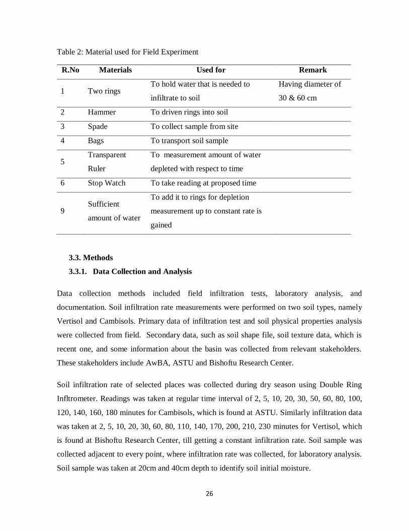
Table 2: Material used for Field Experiment ......................................................................... 26

Table 3: Research Site General Information .......................................................................... 34

Table 4: Calculated Infiltration Parameters of different infiltration models ............................ 51

Table 5: Comparison of Average Observed infiltration and Models Value for Cambisols ...... 54

Table 6: Comparison of Average Observed infiltration and Models Value for Vertisol .......... 55

Table 7: Model Equations for Cambisols and Vertisols ......................................................... 56

Table 8: Infiltration Rate and Cumulative Infiltration Capacity Formulas for Models ............ 57

Table 9: Accuracy Test using Field data Vs Model Values for Cambisols ............................. 58

Table 10: Accuracy Test using Field data Vs Model Values for Vertisol ............................... 59

x

LISTS OF FIGURES

Figures Pages

Fig 1: Typical (a) infiltration rate and (b) cumulative infiltration ............................................. 7

Fig 2: Location Map of Study Site......................................................................................... 25

Fig. 3: Infiltration Rate for Cambisols ................................................................................... 35

Fig 4: Cumulative Infiltration Capacity for Cambisols .......................................................... 36

Fig. 5: Infiltration Rate for Vertisol ....................................................................................... 37

Fig. 6: Cumulative Infiltration Capacity for Vertisol ............................................................. 38

Fig. 7: Average Infiltration Rate and Cumulative Infiltration Capacity for Cambisols ........... 39

Fig. 8: Average Infiltration Rate and Cumulative Infiltration Capacity for Vertisol ............... 40

Fig. 9: Average IR and CI for Cambisols and Vertisol ........................................................... 41

Fig. 10: Graph of Horton for Cambisols (C1, C2, C3, C4, C5 & Average)............................. 43

Fig. 11: Graph of Kostiakov for Cambisols (C1, C2, C3, C4, C5 & Average) ........................ 44

Fig. 12: Graph of Philip for Cambisols (C1, C2, C3, C4, C5 & Average) .............................. 45

Fig. 13: Graph of Green Ampt for Cambisols (C1, C2, C3, C4, C5 & Average) .................... 46

Fig. 14: Graph of Horton for Vertisols (V1, V2, V3, V4, V5 & Average) .............................. 47

Fig. 15: Graph of Kostiakov for Vertisols (V1, V2, V3, V4, V5 & Average) ......................... 48

Fig. 16: Graph of Philip for Vertisols (V1, V2, V3, V4, V5 & Average) ............................... 49

Fig. 17: Graph of Green Ampt for Vertisols (V1, V2, V3, V4, V5 & Average) ...................... 50

Fig. 18: Observed and Model Infiltration Rate for Cambisols ................................................ 52

Graph 19: Observed and Model Infiltration Rate for Vertisol ................................................ 53

xi

LISTS OF ABBREVIATIONS

ANOVA Analysis of Variance

ASTU Adama Science and Technology University

AwBA Awash Basin Authority

CI Cumulative Infiltration

cm Centimeters

DRI Double Ring Infiltrometer

FAO Food and Agriculture Organization

hr Hour

IMC Initial Moisture Content

IR Infiltration Rate

m.a.s.l Meter above Sea Level

MAE Maximum Absolute Error

min Minutes

ml Milliliters

NS Nut-Sutcliffe

NRCS Natural Resource Conservation Service

R2 Coefficient of Determination

RMSE Root Mean Squared Error

SCS Soil Conservation Service

UAB Upper Awash Basin

UN United Nation

UNESCO United Nation Educational, Scientific, and Cultural Organization

xii

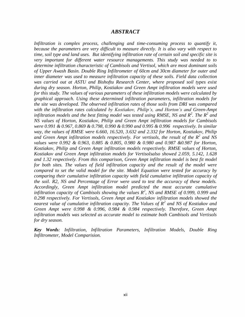
ABSTRACT

Infiltration is complex process, challenging and time-consuming process to quantify it,

because the parameters are very difficult to measure directly. It is also vary with respect to

time, soil type and land uses. But identifying infiltration rate of certain soil and specific site is

very important for different water resource managements. This study was needed to to

determine infiltration characteristic of Cambisols and Vertisol, which are most dominant soils

of Upper Awash Basin. Double Ring Infiltrometer of 60cm and 30cm diameter for outer and

inner diameter was used to measure infiltration capacity of these soils. Field data collection

was carried out at ASTU and Bishoftu Research Center, where proposed soil types exist

during dry season. Horton, Philip, Kostiakov and Green Ampt infiltration models were used

for this study. The values of various parameters of these infiltration models were calculated by

graphical approach. Using these determined infiltration parameters, infiltration models for

the site was developed. The observed infiltration rates of those soils from DRI was compared

with the infiltration rates calculated by Kostiakov, Philip’s, and Horton’s and Green-Ampt

infiltration models and the best fitting model was tested using RMSE, NS and R2. The R

2 and

NS values of Horton, Kostiakov, Philip and Green Ampt infiltration models for Cambisols

were 0.991 & 0.967, 0.869 & 0.798, 0.990 & 0.990 and 0.995 & 0.996 respectively. In similar

way, the values of RMSE were 6.660, 16.520, 3.632 and 2.332 for Horton, Kostiakov, Philip

and Green Ampt infiltration models respectively. For vertisols, the result of the R2 and NS

values were 0.992 & 0.963, 0.885 & 0.805, 0.980 & 0.980 and 0.987 &0.987 for Horton,

Kostiakov, Philip and Green Ampt infiltration models respectively. RMSE values of Horton,

Kostiakov and Green Ampt infiltration models for Vertisolsalso showed 2.059, 5.142, 1.628

and 1.32 respectively. From this comparison, Green Ampt infiltration model is best fit model

for both sites. The values of field infiltration capacity and the result of the model were

compared to set the valid model for the site. Model Equation were tested for accuracy by

comparing their cumulative infiltration capacity with field cumulative infiltration capacity of

the soil. R2, NS and Percentage of Error were used to test the accuracy of these models.

Accordingly, Green Ampt infiltration model predicted the most accurate cumulative

infiltration capacity of Cambisols showing the values R2, NS and RMSE of 0.999, 0.999 and

0.298 respectively. For Vertisols, Green Ampt and Kostiakov infiltration models showed the

nearest value of cumulative infiltration capacity. The Values of R2 and NS of Kostiakov and

Green Ampt were 0.998 & 0.996, 0.984 & 0.984 respectively. Therefore, Green Ampt

infiltration models was selected as accurate model to estimate both Cambisols and Vertisols

for dry season.

Key Words: Infiltration, Infiltration Parameters, Infiltration Models, Double Ring

Infiltrometer, Model Comparision.

1

1. INTRODUCTION

Background of the study, statement of the problem, significance of the study, general and

specific objectives, research questions and scope of the study are described under this part.

1.1. Background of the Study

Infiltration is one part of hydrologic cycle and it is the process by which water on the ground

surface enters the soil profile vertically. In general soil science, infiltration rate is the velocity

or speed at which (rainfall or irrigation) water enters into the soil. It is usually measured by the

depth (in mm or cm) of the water that can enter into the soil per hour (Ayu et al., 2013).

Haghaibi et al., (2011) also said that, infiltration is the process of water movement from the

ground surface into the soil and is an important component in the hydrological cycle.

Infiltration has received a great deal of attention from soil and water scientists because of its

fundamental role in land-surface and subsurface hydrology, irrigation and agriculture (Mishra

et al., 2003). Accurate determination of infiltration rates is an important factor in reliable

prediction of surface runoff (Jagdale et al., 2012).

Infiltration capacity varies in space and time due to soil heterogeneities, meteorological

characteristics, clogging processes and temperature fluctuations, as well as other processes

(Rashidi, et al., 2014). According to Antigha and Essien (2007), variations in the rate of

infiltration are caused by precipitation, land use type, and vegetation type. The characteristics

of the soil also affect the rate of infiltration (Dagadu and Nimbalkar, 2012). Additionally,

David et al., (2018) also stated that infiltration depends upon a large number of factors such as

characteristics of the soil, vegetative cover, condition of the soil surface, soil temperature,

water content of the soil, rainfall intensity, etc.

Infiltration characteristics of the soil are quantified when field infiltration data are fitted

mathematically to infiltration models (Oku and Aiyelari, 2011). According to Rahimi and

Byzedi (2012), infiltration differential equations are of nonlinear kind and they could be

solving as by computer. They concluded that, basic and physical equations of infiltration are

rarely used in designing irrigation systems and the focus is on empirical ones. Ogebe et al.,

(2011) stated that, several studies have been conducted to establish models parameters,

2

validate models or compare models efficiencies and applicability for different soil conditions.

And they investigated the capacity of Kostiakov, Modified Kostiakov, Philip and Horton

infiltration models for sandy soil in central Nigeria and recommend that, Horton‟s models

gave best fit to the measured cumulative infiltration. David et al., (2018) also investigated

infiltration rate capacity of sandy soil using Horton, Green Ampt and Kostiakov infiltration

models and proved that, Kostiakov models is best fit with field observed infiltration rate.

According to Rahimi and Byzedi (2012), Philip model is best fit than Kostiakov,

Kostiakov_Lewis and SCS for clay loam soil. Ramesh et al., (2008) proved that the Horton

Model gives the best representation on the level of infiltration and the time of infiltration on a

variety land use of vertisol soil.

In our country, Ethiopia, there are different soil types which will have different infiltration

capacity and infiltration model efficiencies. According to Upper Awash Sub Basin Integrated

Land Use Planning Study Report (2014), the identified eight FAO major soil groups of Upper

Awash Basin are Vertisols, Luvisols, Cambisols, Nitisols, Andosols, Fluvisols, Regosols, and

Leptosols, including its special distribution. Vertisols are the most extensive soils of the sub

basin; it covers about 40 % of the total area. The distribution of Vertisols is mainly in the

central highland plateaus, or surrounding Finfine zone. The area is known by intensive

cultivation of Teff, Wheat, etc. Nitisols, Luvisols, and Cambisols cover about 27%, their

distribution is mainly in the Northern part. The Fluvisols cover an area of about 2.6% of the

sub basin. Regosols and Leptosols in the sub basin occur mainly, in the eastern part of the sub

basin on steep hill side slopes. They are shallow soils with limited profile development and

they cover an area about 14% of the sub basin. Andosols are mainly occurring in volcanic

areas around Sodere and Metehara, they cover about 9.3%.

Even though there are many findings that are related to soil infiltration rate of different area,

yet, there is no scientific study that shows infiltration capacity of upper Awash Basin of

Ethiopia. Since competition of the available water resources from different use is very high in

upper awash basin, major soil infiltration rate of the basin is very important to plan and

manage the water resource of the basin.

3

1.2. Statement of the Problem

Applying infiltration equations in modeling of both surface and subsurface flows results in

easier surface irrigation systems designing and evaluating. Due to the correlation between the

coefficients of the equations and type of soil and surface conditions exacting field tests seems

to be really necessary. The infiltration rate into the soil in one of the important parameters in

designing and performing irrigation and drainage projects, hydrological studies, soil

conservation and water supply management, designing and performing green areas, soil pools

of fish farming etc (Rahimi and Byzedi, 2012). Arshad et al., (2015) and Ieke et al., (2013)

stated that, infiltration plays an important role in generation of runoff volume and modeling of

this surface runoff.

So, infiltration is the most important process in hydrologic processes. All flooding, erosion,

irrigation scheduling, identification of recharge area and pollutant transportation predictions

are depends on infiltration. But this important process, infiltration, is vary temporary and

spatially. Therefore, for accurate quantification of this process in-situ, the development of

models for specific time and space is paramount. Even though, infiltration process determines

these different hydrologic processes, yet, there is no study that shows infiltration rate of most

dominant soil of upper awash basin.

Regardless of this, there is the fact that, because of the rapid population growth and increased

water demand of different sectors in the last few years, the water resource in the basin has

become issues of concern and source of conflicts. Irrigation sector is one of the sectors

competing for water. To allocate water for irrigation, identifying soil infiltration capacity and

climate condition is mandatory. Over- and inefficient utilization triggered by no or limited

knowledge of the water resources availability regardless of the spatial and temporal

distribution is significantly facilitating competition and conflicts for water in the basin (Awash

Basin Water Allocation Plan, 2016). Despite of these facts, till today, no clear finding exist

that shows infiltration capacity Cambisols and Vertisols of the area.

And therefore this study was conducted to identify infiltration capacity of the soils and to

select best fit infiltration model for the site was done. Specially, this study has great role for

irrigation water management.

4

1.3. Significance of the Study

Soil and water are the vital natural resources used in the crop production system. Efficient

management of water requires a greater control of infiltration in the soil. Increased infiltration

control would help to solve such wide range of problems as upland flooding, pollution of

surface and groundwater, declining water tables, inefficient irrigation of agricultural lands, and

wastage of useful water (Rashidi et al., 2014). Soil infiltration rate is the most essential

process that affects the surface irrigation uniformity and efficiency because of its mechanism

of transfer and distributes water from surface to soil profile (Rashidi et al., 2014).

Adequate knowledge of infiltration rate of different soils is very essential for water resource

management. Moreover, prediction of cumulative infiltration is important for estimation of the

amount of water entering and its distribution in the soil. Design, operation, management, and

hydraulic evaluation of on-farm water applications have also rely on the infiltration properties

of the soil because infiltration behavior of the soil directly determines the essential variables

such as inflow rate, length of run, application time, depth of percolation, and tail water run-off

in irrigation systems (Sarmadian and Mehrjardi, 2014). Therefore, the result of the study has

vital role for irrigation water management, selection and design of irrigation type and

irrigation structures. It will be used for water harvest and runoff prediction too.

1.4.Objective of the Study

1.4.1. General objective

The main objective of this study was to determine infiltration capacity of Cambisols and

Vertisols.

1.4.2. Specific objectives

i. To quantify the values of different infiltration models parameters

ii. To compare the performance of different infiltration models

iii. To set infiltration equations for Cambisols and Vertisols

iv. To test accuracy of infiltration models

1.5. Research Questions

The study contains the following research questions

5

What are the values of different infiltration parameters for the site?

Which infiltration model has close relationship with field infiltration data?

Which infiltration model is accurate to predict infiltration capacity of the soil?

1.6. Delimitation/Scope

According to Upper Awash Basin Integrated Land Use Planning Study (2014), Vertisols,

Luvisols, Cambisols, Nitisols, Andosols, Fluvisols, Regosols, and Leptosols, are found to be

major soil groups of Upper Awash Basin. Even though different soil types result different

infiltration rates, this study is limited only to Vertisol and Cambislos, which are most

dominant, because of time and cost constraint. For this study, representative data were

collected from two selected sites of Upper Awash Basin, Adama Science and Technology

University and Bishoftu Research Center.

According to Upper Awash Basin Integrated Land Use Planning Study, the land

cover/vegetation cover types identified in the Upper Awash sub-basin includes Afro-Alpine

and Sub Afro-Alpine vegetation, Cultivated Land, Forest Land, Grass Land, Shrub Land,

Water body, Wood land, bare land. A large proportion of the sub basin is accounted as

cultivated land, Forest Land, Grass Land and Water body. From these land uses of Upper

Awash basin, only agricultural land was tested for soil infiltration rate using DRI since Upper

Awash basin, which has about 68% flat landscape to gently undulating, was selected for this

research. And also, from wet and dry seasons, only dry season was selected for this research

due to time and budget.

6

2. LITERATURE REVIEW

In this part, the review of different theoretical approaches and related studies by scholars that

have relation with infiltration and infiltration rates are described.

2.1. Theoretical Approaches of Infiltration and Infiltration Rates

2.1.1. Water and Soil

Lal and Shukla (2005), stated that, from the sum of all water bodies (oceans, rivers, lakes),

groundwater (renewable and fossil), and soil water, about 97.2% (volume basis) of the

world water is in oceans and seas. Fresh water accounts for merely 2.8% of the total

volume, of which groundwater is 0.6% and soil water accounts for less than 0.1% of the

total.

According to Miyazaki (2006), property of water in soils differs a little from that of ordinary

water. Even when pure water is added to a dry soil, absorbed materials on particle surfaces

may be dissolved in the penetrating water, and hence the water is no longer pure but will

behave as a solution. A solution that dissolves cations and anions is affected by the negative

charge on the surface of clay minerals, resulting in diffuse electrical double layers around the

clay minerals due to the attraction of cations and the repulsion of anions.

Freud and Rahardjo (1993), describe water movement in soil clearly. The slow movement of

water through soil is commonly referred to as seepage or percolation. Seepage analyses may

form an important part of studies related to slope stability, groundwater contamination control,

and earth dam design. Seepage analyses involve the computation of the rate and direction of

water flow and the pore-water pressure distributions within the flow regime.

The flow of water in the saturated zone has been the primary concern in conventional seepage

analyses. However, water flow in the unsaturated zone is of increasing interest to engineers. A

constant water flux across the surface boundary may develop a steady-state water flux through

the unsaturated zone of the slope. Water flow through unsaturated soils is governed by the

same law as flow through saturated soils (Le. Darcy's law). The main difference is that the

water coefficient of permeability is assumed to be a constant for saturated soils, while it must

be assumed to be a function of suction, water content, or some other variable for unsaturated

7

soils. Also, the pore-water pressure generally has a positive gauge value in a saturated soil and

a negative gauge value in an unsaturated soil. In spite of these differences, the formulation of

the partial differential flow equation is similar in both cases.

2.1.2. Infiltration and Infiltration Models

According to Lal and Shukla (2005), entry of water into the soil matrix through air-soil

interface is called infiltration. The water entry is generally referred to as vertical downward

infiltration. The rate of infiltration of water into soil matrix governs the amount of water

storage in soil, which is available for plants. It also influences the amount of runoff and

erosion. And the book recommended that the knowledge of water infiltration into soil is

essential for soil and water conservation, and minimizing the risk of nonpoint source pollution.

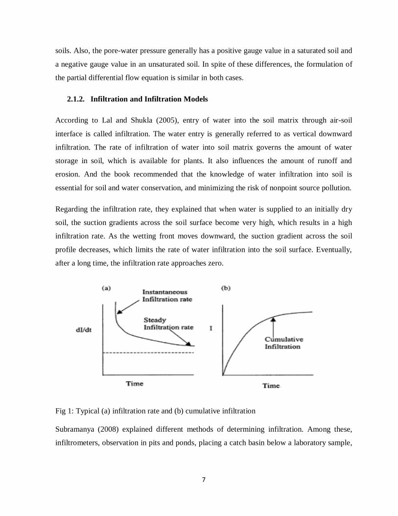
Regarding the infiltration rate, they explained that when water is supplied to an initially dry

soil, the suction gradients across the soil surface become very high, which results in a high

infiltration rate. As the wetting front moves downward, the suction gradient across the soil

profile decreases, which limits the rate of water infiltration into the soil surface. Eventually,

after a long time, the infiltration rate approaches zero.

Fig 1: Typical (a) infiltration rate and (b) cumulative infiltration

Subramanya (2008) explained different methods of determining infiltration. Among these,

infiltrometers, observation in pits and ponds, placing a catch basin below a laboratory sample,

8

artificial rain simulators and hydrograph analysis are common. Double ring infiltrometer is

most common method used for soil infiltration rate test in field.

2.1.3. Darc’s Law of Water Flow in Soil

Miyazaki (2006) explained Darc‟s law for liquid flow in soil as follows. Liquid water flows

through continuous and tortuous pores in soils. Darcy‟s law is a macroscopic law deduced by

the integration of the individual water flow in each pore, which has various shapes

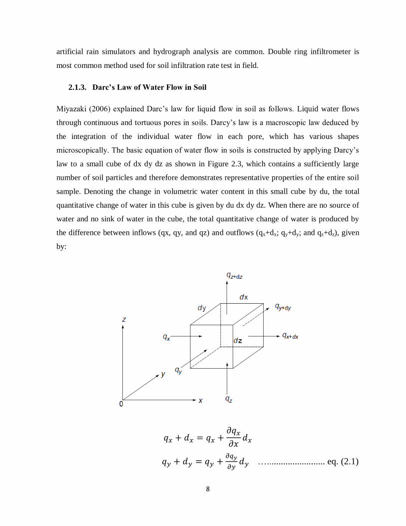
microscopically. The basic equation of water flow in soils is constructed by applying Darcy‟s

law to a small cube of dx dy dz as shown in Figure 2.3, which contains a sufficiently large

number of soil particles and therefore demonstrates representative properties of the entire soil

sample. Denoting the change in volumetric water content in this small cube by du, the total

quantitative change of water in this cube is given by du dx dy dz. When there are no source of

water and no sink of water in the cube, the total quantitative change of water is produced by

the difference between inflows (qx, qy, and qz) and outflows (qx+dx; qy+dy; and qz+dz), given

by:

…......................... eq. (2.1)

9

The continuity equation of water during a given time dt is then given by

…..… eq. (2.2)

Which results in

(

) ………………………………………………eq. (2.3)

Applying Darcy‟s law

(

)

(

)

(

) …………………...………eq. (2.4)

2.2.Some Scientific Studies Related to Infiltration Rates

2.2.1. Horton Infiltration Model

Ayu et al., (2013) studied infiltration capacity using Horton infiltration model. The scholars

used Double Ring Infltrometer and collected data using field observations, interviews, and

documentation. The simple random sampling was used to determine locations for infiltration

measurement. Soil sampling and measurement of infiltration were performed on three

different land uses with six replications in each location.

The researchers estimated the value of fc from plotting of the relationship between the

infiltration rate and time and the result showed that there are different infiltration rates for

different land uses. According to the researchers, soil properties affecting infiltration rate in

the research locations were sand and clay percentages, soil moisture content, bulk density,

particle density, soil organic matter, and soil porosity. Finally, the scholars concluded that

estimated value of soil infiltration using Horton Model was similar with the value of

infiltration measurement in the field.

Abdulkadir et al., (2011) also used Horton infiltration model to test 15 points of infiltration

by ponding water into a double ring infltrometer and readings was recorded at 1 minute

intervals for the first 5 minutes, 5 minutes intervals for the next 50 minutes, 10 minutes

intervals to 60 minutes then 20 minutes intervals for the next 60 minutes until a total elapsed

10

time of 120 minutes was reached. To determine infiltration parameters, Horton infiltration

model was used.

They concluded that calculated infiltration rates by Horton Model was similar to those from

field measurements and the Horton equation was best explained in the exponential curve

fitting technique. There was a good relationship between the measured and predicted

infiltration rates with mean R2 value of 0.811 for all 15 sample points.

2.2.2. Kostiakov Infiltration Model

Hasan et al., (2015) had done the research at dry season using Double Ring Infltrometer. The

modified Kostiakov method was tested if it suits the local soil condition and if it can be

represented for the accumulated infiltration and infiltration rate. The finding showed that very

good agreement between the actual and calculated values of accumulated infiltration. The

scholars agreed that, this will also be a good representative of the infiltration characteristic of

the site. Finally, they recommended that this information can be valued asset for irrigation

scheduling for any crop cultivated in that field to ensure the best water management practices.

Uloma et al., (2014) also made field infiltration measurements using double ring infiltrometer

during wet season. Repeated readings were taken at 5, 10, 15 and 30 minutes intervals in all

the locations and Kostiakov‟s equation was used. The scholars agreed that, infiltration rates

(IR) values were low and this is attributed to the high moisture content of the soil since the

experiments were conducted in rainy (wet) season.

2.2.3. Philip Infiltration Model

Singh et al., (2014) evaluated infiltration capacity of soil of nine different locations using

double ring infltrometer. The Infiltration rate mm/hr and measured data F(t) were plotted in

graph and the method of nonlinear regression is applied to find out unknown parameter K and

S of Philip infiltration model.

Scholars observed that there is a lot of variation in the infiltration rate from time to time. They

recommended that, it is mainly due to the meteorological properties also. And the result

showed that initial infiltration rate is very high and after 60 minutes the infiltration rate is low.

11

There was also large variation in infiltration parameter particularly saturated hydraulic

conductivity. The researchers concluded that it is noted that different infiltration rates are

observed for same soil due to the variation in water content.

2.3.Comparison of Different Infiltration Models

Ogbe et al., (2011) carried out field experiment at the College of Agriculture experimental

farm, Lafia. Three points at 30m interval the length was marked out and infiltration test

carried out at those points for each strip. Soil samples were also collected from the adjacent

area of the marked points at different depths for soil analysis. Infiltration measurement was

carried out using a double ring infltrometer. Readings were then taken at intervals to

determine the amount of water infiltrated during the time interval with an average infiltration

head of 5cm maintained. The infiltration rate and the cumulative infiltration were then

calculated. Moisture content was determined by gravimetric method. The soil texture of the

site was determined by mechanical analysis method.

Several models including Kostiakov, Modified Kostiakov, Philip and Horton models have

been developed for monitoring infiltration process. The cumulative infiltration values

predicted using the infiltration models and those measured were plotted against each other and

fitted with a linear equation with zero intercept to verify the validity of each prediction. The

slope of the line of best fit and its coefficient of determination (R2) for each model and strip

were given. Statistical results indicates that all the models used satisfactorily predicted the

cumulative infiltration given that the t-calculated values for all the models in each strip are

less than the t-table value. Therefore, it can be concluded that the field measured cumulative

infiltration do not differ from those predicted by the models since the observed difference can

be accounted for by experimental error.

They concluded that, from the four infiltration models evaluated, the Horton‟s models gave

best fit to the measured cumulative infiltration, although the other models provided good

overall agreement with the field measured cumulative infiltration depths and are therefore

capable of simulating infiltration under the field conditions encountered in the present study.

Consequently, the application of these equations under verified field conditions leads to the

12

determination of the appropriate infiltration characteristics for the equations that would

optimize infiltration simulation, irrigation performance and minimize water wastage.

Sreejani et al., (2017) also used Double ring infltrometer for measurement of infiltration rates

at all the sites and readings were taken at regular time interval of 2, 5, 10, 15, 30, 60 min. till

getting a constant infiltration rate. Then the values of various constants of the models were

calculated by graphical approach. To get best fitting model for a particular soil condition the

results obtained from various infiltration models were compared with observed field data and

graphs are drawn with correlation coefficient and standard error as tools.

The researchers got that the values of parameters of Infiltration models vary from soil to soil

and from place to place. From the analysis they concluded that, for all regions selected in the

study area, Kostiakov‟s Model was best fitting with high degree of Correlation Coefficient and

Minimum standard Error.

Arshad et al., (2016) conducted research to analyze the water transmission behavior for sandy

loam soil under different tillage operations of Raja MB Plough and its comparison with

different infiltration models. The results were found that the values of parameters regarding

infiltration rate and cumulative infiltration vary from unploughed soil to the ploughed soil

with different number of tillage operations of Raja MB plough. The statistical data and various

infiltration models results showed different results for each tillage operation.

From their analysis, they found that initially infiltration rates were high in all experiments and

decreased with time up to steady infiltration rate base flow acquired. And finally they

concluded that, there was a strong correlation of field data with Horton‟s model and hence, it

is concluded that Horton‟s model is appropriate model with high significant results of

correlation coefficient and minimum standard error.

David et al., (2018) used double ring Infiltrometer which consists of two cylinders which has

diameter of the inner ring is 30 cm and that of outer ring is 60 cm to collect field infiltration

rate. The researchers used three statistical parameters such as one way ANOVA test,

correlation coefficient and standard error for comparing the observed values of infiltration rate

with the Horton model, Green ampt model and Kostiakov model infiltration models. And they

13

concluded that Kostiakov‟s model is the best fit model with observed infiltration rate for the

site.

Rahimi and Byzedi (2012) calculated Kostiakov, Kostiakov - Lwies, SCS and Philip's

infiltration equations coefficients and integrated infiltration equations infiltration rate and

average infiltration rate by practicing the best empirical data graph. The researchers found

that, K coefficient in Kostiakov equation is its proximity to S or absorption coefficient in

Philip's equation which shows the dependency of K coefficient on physical characteristics of

soil. They concluded that, Philips model estimates integrated infiltration and infiltration rate

with high precise and the SCS model underestimated integrated infiltration and infiltration rate

in all condition so it is not recommended for the area.

So, they recommended that, the best model for estimating the integrated infiltration and

infiltration rate for agricultural fields of the area and similar fields is the Philips model and

therefore, obtained results of this model can be used for estimating the integrated infiltration

and infiltration rate in designing surface irrigation systems (except furrow irrigation method)

and other given objectives.

Sihag et al., (2017) used Double ring Infiltrometer for measurement of infiltration rates at all

selected locations. They proposed models such as Kostiakov, Kostiakov modified, SCS and

the novel for evaluation in the study. The researchers evaluated these infiltration models on

the basis of experimental data of the study area and to obtain numerical values for the

parameters of the models using XLSTAT software. To compare infiltration models, Maximum

Absolute Error (MAE), Bias and Root Mean Square Error (RMSE) statistical criteria was used

by researchers. According to these statistical criteria, they concluded that, the novel model is

performing better than other models and it may be used to assess the infiltration rate with

similar field characteristics of the site.

Dagadu and Nimbalkar (2012) compared infiltration models For black cotton soil, three

regions were selected in which first region was of compact soil type, second region was

ploughed, and third was of harrowed condition. Two regions were selected for clay soil, of

which first was unploughed condition and second was ploughed condition. For sandy soil one

region was selected. From the results, they found that, the values of parameters of infiltration

14

models vary from soil to soil and soil type. Also the correlation coefficients and standard

errors were different for different soils and different soil conditions.

Finally the researchers concluded that, from the correlation coefficient and standard error

calculations it was found that for all type of soils and their conditions Horton‟s model is best

fitting with high degree of correlation coefficient and minimum standard error except for

ploughed clay soil to which Green_Ampt model is best fitting. So from the study it is

concluded that Horton‟s model is best fitting with measured values of infiltration rates for all

types of soils and soil conditions except for ploughed clay soil in the region.

Nitin P Sonaje (2017) reviewed methods for estimation of water infiltration rate such as, In

situ measurement techniques, Empirical models, Green-Ampt models, Richard‟s equation

models.

The researcher stated that in situ measurement technique includes be measured or estimated

either by measurement on undisturbed samples in laboratory or in situ measurements. The DRI

is used for measuring cumulative infiltration, infiltration rate and field-saturated hydraulic

conductivity. And he concluded that in situ measurement techniques have some limitations

such as rate of infiltration decreases with increase in the depth and rate of infiltration increases

with increase in head of water, boundary condition of infiltrometer effect on rate of infil-

tration, the driving of tube or rings disturbs the soil structure; and raindrop-impact is not

simulated and Complex and less accurate

The Author agreed that, empirical models are usually in simple form of equations when

compared with in situ method and they provide estimates of cumulative infiltration and

infiltration rates quite accurately. However, they are unable to provide information regarding

water content distribution. The empirical models that reviewed by the Author includes

Kostiakov, Modified Kostiakov, Horton, Philip, Mezencev and Holtan models.

The researcher identified that, Kostiakov model describes the infiltration quite well at small

time but less accurate at large times. It was further modified as Modified Kostiakov‟s

Equation which is most commonly used in surface irrigation applications. Horton‟s Equation

is the theory proposed by Horton (1940) describes the basic behavior of infiltration but the

15

physical interpretation of exponential constant is poorly defined. The researcher identified

that, the striking drawback of this equation is inadequacy to represent the rapid decrease of „i‟

from very high values at „t‟ as shown by Philip. And he stated that Philip equation is valid in

the limiting condition of „t‟ not being too large. The limitations of Kostiakov‟s equation for

large times, was modified by Mezencev. NRCS (SCS) Equation assumes that for a single

storm, ratio of actual soil retention to potential maximum retention is equal to the ratio of

direct runoff to available rainfall. In case of lack of soil moisture data or insufficient definition

of boundary conditions, the NRCS model is suitable semi-empirical model. Holtan model

specifically takes into account the effects of vegetation and soil water condition in the form of

available pore space for moisture storage.

Being widely-accepted concepts of soil physics and easy to use, easily obtained hydraulic

parameters from literature and electronic databases, no need of site-specific measurements of

all parameters, easily incorporation of spatial variability of soil parameters can be more into

the mathematical models are some advantages of empirical models stated by the author.

The researcher stated that, Green Ampt model is the model which addresses surface ponding

and movement of wetting front. According to the researcher, the core importance in this

method is evaluation of soil moisture-pressure profile. Simplicity to use, Adaptability to

varying scenarios, Easily-measurable variables are advantages of Green Ampt Model.

Depending on the simplicity (or complexity) of input parameters, Richard‟s equation has been

solved exactly or partially. Limitations of Richard Equation includes colloidal swelling and

shrinking of soils may demand that the water movement be considered relative to the move-

ment of soil particles; this phenomenon may also cause significant changes in soil

permeability, two-phase flow involving air movement may be important when air pressures

differ significantly from atmospheric pressure, thermal effects may be important, especially

for evaporation during redistribution of infiltrated water, in which case the simultaneous

transfer of both heat and moisture needs to be considered and depending on the simplicity (or

complexity) of these input parameters, the Richards equation can be solved exactly or

numerically.

16

2.1. Spatial and Temporal Variation of Infiltration Rate

Balstad et al., (2018) investigated the design implications of seasonal variations in infiltration

capacity, simulations of a typical rain garden located in Trondheim. The results presented in

this paper indicated that, large seasonal variations in infiltration capacity. The infiltration

capacity changed from 1 cm/h in October too close to 0.05 cm/h in November- April and up to

3 cm/h in May.

Eze et al., (2011) computed mean infiltration rate for bare and crusted, sparsely vegetated with

50cm depth of litter cover. “Crust Factor” was calculated using the ratio of the steady state

infiltration rate of bare surface divided by the steady state infiltration rate of vegetated soils.

The result posited that infiltration rates for vegetated surface were higher than those of the

bare crusted and sparsely vegetated surfaces. It implies that the vegetated land use contributes

better to soil protection against surface runoff and erosion than bare crusted and sparsely

vegetated surface in the study area. The research also revealed that porosity is a measure of the

water bearing capacity of a soil and it plays a role in the determining the capability of the soil

to transmit water Calculating the “crust factor” which is the ratio of the infiltration rate of the

bare and crusted surface to that of vegetated surface it gave a value of 0.0530.

The research showed that vegetation cover is one of the most important factors that accelerates

infiltration rate and thus reduces overland flow which and ultimately in turns conserves the

soil. From the analysis, they concluded that, the area is unsuitable for surface irrigation due to

its high infiltration capacity. They also recommended that human activities in the form of

deforestation, bush burning and grazing by livestock should be discouraged, while in this area;

planting of trees on bare lands should be encouraged to reduce erosion.

Vianová et al., (2011) carried out evaluation of soil infiltration capacity at both sites of

interest on the basis of data acquired during the on-site infiltration tests and processed in

compliance with Kostiakov‟s method. 24 tests were carried out in total, each time three tests

took place at each site. Infiltration characteristics were assessed with regard to soil physical

properties, changing properties during the reference period. The finding showed that

infiltration capacity of the soil, at both sites, is low at rainy time and compaction places and

high at dry season. Depending on the time of measurement the result shows that soil

17

infiltration capacity was lower in spring and autumn and higher in summer (until harvest of

the grown crop-plant) due to higher initial moisture content of the soil. Finally, the scholars

concluded that Soil compaction is a problem that manifests itself not only by reduced

infiltration capacity of soils, but also causes many other phenomena having a negative

influence on the overall soil quality and fertility.

Patle et al., (2018) identified twenty five points at 10 m grid interval and field measurements

were performed using DRI. A soil sample was collected for estimating: Soil Moisture, Bulk

Density, Particle Density and Texture and organic carbon content. The coefficient of

determination was also determined to check reliability of the model.

The relationship between infiltration rate and each soil properties were analyzed and it is seen

that sand, particle density, and organic content had positive correlation with observed

infiltration rate which means increase in sand, particle density, and organic content will

increase the infiltration rate. Silt, clay, bulk density, and moisture content had a negative

correlation with infiltration rate which means that increasing silt, clay, bulk density, and

moisture content will decrease infiltration rate.

2.2. Accuracy Test for Infiltration Models

Arshad et al., (2015) investigated the effect of tillage intensity to the water transmission

behavior for sandy loam soil in terms of infiltration rates and cumulative infiltration and its

validation with different infiltration models. The scholar used to compare observed cumulative

infiltration and model cumulative infiltration for model validation. Standard Deviation,

Standard Error and Coefficient of determination was used for comparison. Finally, the scholar

concluded that Horton infiltration model is accurate model for the site.

The accuracy of the different equations for predicting the cumulative infiltration were

evaluated by comparing the observed values of measurement on the field and the predicted

values based on the fitted equation. The cumulative infiltration values predicted using the

infiltration models and those measured were plotted against each other and fitted with a linear

equation with zero intercept to verify the validity of each prediction. The slope of the line of

best fit and its coefficient of determination (R2) for each model. To check the discrepancies

18

between the predicted and the measured values, paired t-test and Root Mean Square Error

(RMSE) were used. Considering the four infiltration models evaluated, the Horton‟s models

gave best fit to the measured cumulative infiltration, although the other models provided good

overall agreement with the field measured cumulative infiltration depths (Ogbe et al., 2011)

2.3. Soil Classification

According to FAO (2001), Soil Map of the World was published 1974. Compilation of the

Soil Map of the World was a formidable task involving collection and correlation of soil

information from all over the world. Initially, the Legend to the Soil Map of the World

consisted of 26 („first level‟) “Major Soil Groupings” comprising a total of 106 („second

level‟) „Soil Units‟.

In 1990, a „Revised Legend‟ was published and a third hierarchical level of „Soil Subunits‟

was introduced to support soil inventory at larger scales. Soil Subunits were not defined as

such but guidelines for their identification and naming were given. In 1998, the International

Union of Soil Sciences officially adopted the World Reference Base for soil resources as the

union‟s system for soil correlation. The structure, concepts and definitions of the world

reference base are strongly influenced by the Food and Agriculture Organization -UNESCO

soil classification system. At the time of its inception, the world reference base proposed 30

„Soil Reference Groups‟ accommodating more than 200 („second level‟) Soil Units.

19

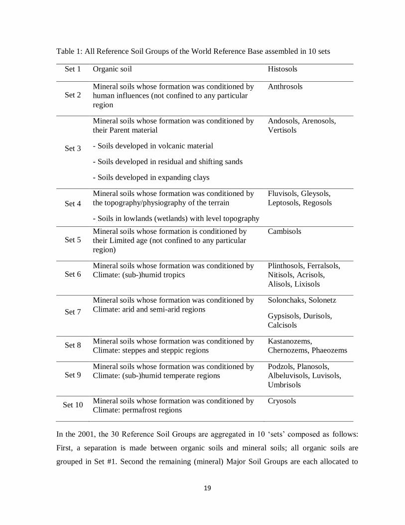
Table 1: All Reference Soil Groups of the World Reference Base assembled in 10 sets

Set 1 Organic soil Histosols

Set 2 Mineral soils whose formation was conditioned by

human influences (not confined to any particular

region

Anthrosols

Set 3

Mineral soils whose formation was conditioned by

their Parent material

- Soils developed in volcanic material

- Soils developed in residual and shifting sands

- Soils developed in expanding clays

Andosols, Arenosols,

Vertisols

Set 4


the topography/physiography of the terrain

- Soils in lowlands (wetlands) with level topography

- Soils in elevated regions with non-level

topography

Fluvisols, Gleysols,

Leptosols, Regosols

Set 5 Mineral soils whose formation is conditioned by

their Limited age (not confined to any particular

region)

Cambisols


Climate: (sub-)humid tropics

Plinthosols, Ferralsols,

Nitisols, Acrisols,

Alisols, Lixisols

Set 7


Climate: arid and semi-arid regions

Solonchaks, Solonetz

Gypsisols, Durisols,

Calcisols


Climate: steppes and steppic regions

Kastanozems,

Chernozems, Phaeozems


Climate: (sub-)humid temperate regions

Podzols, Planosols,

Albeluvisols, Luvisols,

Umbrisols


Climate: permafrost regions

Cryosols

In the 2001, the 30 Reference Soil Groups are aggregated in 10 „sets‟ composed as follows:

First, a separation is made between organic soils and mineral soils; all organic soils are

grouped in Set #1. Second the remaining (mineral) Major Soil Groups are each allocated to

20

one of nine sets on the basis of „dominant identifiers‟, i.e. those soil forming factor(s) which

most clearly conditioned soil formation.

From these sets, Food and Agriculture Organization describes vertisol and Cambisols, which

are major soils Upper Awash Basin, were selected for the evaluation of infiltration rate. And

infiltration models were developed for these two major soil types. The detail description of

these soil types are described below.

2.3.1. Vertisols

Vertisols are churning heavy clay soils with a high proportion of swelling 2:1 lattice clays.

These soils form deep wide cracks from the surface downward when they dry out, which

happens in most years. The name Vertisols (from L. vertere, to turn) refers to the constant

internal turnover of soil material. Some of the many local names became internationally

known, e.g. „black cotton soils‟ (USA), „regur‟ (India), „vlei soils‟ (South Africa), „margalites

(Indonesia), and „gilgai‟ (Australia).

According to Food and Agriculture Organization report, Vertisols cover 335 million hectares

world-wide. An estimated 150 million hectares is potential cropland. Vertisols in the tropics

cover some 200 million hectares; a quarter of this is considered to be „useful‟. Most Vertisols

occur in the semi-arid tropics, with an average annual rainfall sum between 500 and 1000 mm

but Vertisols are also found in the wet tropics, e.g. in Trinidad where the annual rainfall sum

amounts to 3000 mm. The largest Vertisol areas are on sediments that have a high content of

smectitic clays or produce such clays upon post-depositional weathering (e.g. in the Sudan)

and on extensive basalt plateaux (e.g. in India and Ethiopia). Vertisols are also prominent in

Australia, southwestern USA (Texas), Uruguay, Paraguay and Argentina.

Food and Agriculture Organization report indicate that, infiltration of water in dry (cracked)

Vertisols with surface mulch or a fine tilth is initially rapid. However, once the surface soil is

thoroughly wetted and cracks have closed, the rate of water infiltration becomes almost zero.

(The very process of swell/shrink implies that pores are discontinuous and non-permanent.) If,

at this stage, the rains continue (or irrigation is prolonged), Vertisols flood readily. The highest

infiltration rates are measured on Vertisols that have a considerable shrink/swell capacity, but

21

maintain a relatively fine class of structure. Not only the cracks transmit water from the (first)

rains but also the open spaces between slickensided ped surfaces that developed as the peds

shrunk.

According to Upper Awash Basin Integrated Land Use Planning Study Report (2014),

Vertisols are the most dominant and important soils of the Upper Awash sub basin and they

cover an area about 774,156 ha or 40%. The report stated that, the soils of this category are,

very deep and uniformly thick consisting of dark grey or very dark grayish brown color and

during the dry season these soils develop cracks.

2.3.2. Cambisols

The Reference Soil Group of the Cambisols holds soils with incipient soil formation.

Beginning transformation of soil material is evident from weak, mostly brownish

discolouration and/or structure formation below the surface horizon. Cambisols cover an

estimated 1.5 billion hectares worldwide. This Reference Soil Group is particularly well

represented in temperate and boreal regions that were under the influence of glaciation during

the Pleistocene, partly because the soil‟s parent material is still young but also because soil

formation is comparatively slow in the cool, northern regions. Erosion and deposition cycles

account for the widespread occurrence of Cambisols in mountain regions (FAO, 2001).

According to FAO (2001), Cambisols are also common in areas with active geologic erosion

where they may occur in association with mature tropical soils. FAO (2001) satated that

Cambisols make good agricultural land and are intensively used. The Eutric Cambisols of the

Temperate Zone are among the most productive soils on earth. The Dystric Cambisols, though

less fertile, are used for (mixed) arable farming and as grazing land. Cambisols on steep slopes

are best kept under forest; this is particularly true for Cambisols in highlands. Vertic and

Calcaric Cambisols in (irrigated) alluvial plains in the dry zone are intensively used for

production of food and oil crops. Eutric, Calcaric and Chromic Cambisols in undulating or

hilly (mainly colluvial) terrain are planted to a variety of annual and perennial crops or are

used as grazing land. Dystric and Ferralic Cambisols in the humid tropics are poor in nutrients

but still richer than associated Acrisols or Ferralsols and they have a greater cation exchange

capacity.

22

Upper Awash Basin Integrated Land Use Planning Study Report (2014) showed that, these

major soil units are well, to somewhat excessively drained, deep, and light to medium

textured, with variable colors. The soils are formed on a wide range of parent materials. The

soils have a moderately developed subsoil horizon, which is only at initial stage of

development. Structure is weak to strongly developed angular blocky, occasionally prismatic

in the topsoil over moderate angular blocky to massive in the subsoil. Consistence is hard

when dry, friable to firm when moist and slightly sticky and slightly plastic when wet. The

study identified that, Cambisols are the widely distributed soils in the sub basin; they cover

about 313,033 ha or 16% . These soils are sub classified as Chromic, Vertic, Calcaric, and

Eutric Cambisols.

23

3. MATERIALS AND METHODS

This part contains detail description of study area, material used for the study, methods

followed to collect and analysis soil infiltration data.

3.1. Description of the Study Area

3.1.1. Location and Description

The Awash basin is part of the Great Rift Valley in Ethiopia which is located from latitude

8.50 N to 12

0N and longitude: 38° to 41.8° E, altitude: 250-3927 m.a.s.l. It covers a total area

of 110,000 km2 of which 64,000 km

2 comprises the Western Catchment, drains to the main

river or its tributaries. The remaining 46,000 km2, most of which comprises the so called

Eastern Catchment, drains into a desert area and does not contribute to the main river course.

The river rises on the High plateau near Ginchi town west of Addis Ababa in Ethiopia and

flows along the rift valley into the Afar triangle, and terminates in salty Lake Abbe on the

border with Djibouti.

Based on physical and socio-economic factors, the Awash Basin is divided into Upper Awash,

Middle Awash, Lower Awash and Eastern Catchment. The Upper, Middle and Lower Valley

are part of the Great Rift Valleys systems (Awash Basin Water Allocation Plan, 2016).

According to Upper Awash Sub Basin Integrated Land Use Planning Study, Upper Awash

sub-basin is limited on the upper part of the Awash River basin, which extended from the head

up to Arba River within Fentale district and clipped by the boundary of Oromia Regional

State. The study showed that, the geographical extent of the Upper Awash Basin ranges from

7053‟44.55” N to 9

024‟05.36” N and 37

056'43

.24

”E to 40

010'50.74”E. And the study showed

that Vertisols are the most extensive soils of the sub basin; they cover about 40 % of the total

area while Nitisols, Luvisols, and Cambisols cover about 27%. Regosols and Leptosols in the

sub basin cover an area about 14% of the sub basin.

The land cover/vegetation cover types identified in the Upper Awash sub-basin includes Afro-

Alpine and Sub Afro-Alpine vegetation, Cultivated Land, Forest Land, Grass Land, Shrub

Land, Water body, Wood land, bare land. A large proportion of the sub basin is accounted as

24

cultivated land, Forest Land, Grass Land, Water body also consumable significant in the sub-

basin.

The experiments were carried out at Adama Science and Technology University and Bishoftu

Research Center. Adama Science and Technology University is located in Adama town where

Leptosols, Andosols and Cambisols exist. The land cover of Adama Science and Technonlogy

are grass land, forest, residential, agricultural land and paved land. From these land use land

covers, agricultural land was used for the research.

Bishoftu Research Center was established under Haramaya University in 1953 and transferred

to Ethiopian Agricultural Research Organization in 1984. It has total area of 147 hectares.

Vertisols, Leptosols and Cambisols are major soil types that exist in the research center.

Vertisols are most dominant soils that cover 127 hectares which is 86% from the total area.

25

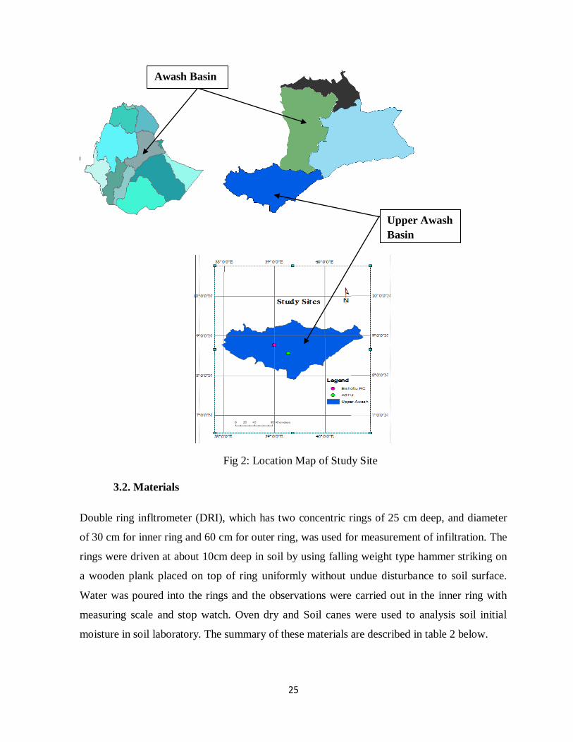
Fig 2: Location Map of Study Site

3.2. Materials

Double ring infltrometer (DRI), which has two concentric rings of 25 cm deep, and diameter

of 30 cm for inner ring and 60 cm for outer ring, was used for measurement of infiltration. The

rings were driven at about 10cm deep in soil by using falling weight type hammer striking on

a wooden plank placed on top of ring uniformly without undue disturbance to soil surface.

Water was poured into the rings and the observations were carried out in the inner ring with

measuring scale and stop watch. Oven dry and Soil canes were used to analysis soil initial

moisture in soil laboratory. The summary of these materials are described in table 2 below.

Awash Basin

Upper Awash

Basin

26

Table 2: Material used for Field Experiment

R.No Materials Used for Remark

1 Two rings To hold water that is needed to

infiltrate to soil

Having diameter of

30 & 60 cm

2 Hammer To driven rings into soil

3 Spade To collect sample from site

4 Bags To transport soil sample

5 Transparent

Ruler

To measurement amount of water

depleted with respect to time

6 Stop Watch To take reading at proposed time

9 Sufficient

amount of water

To add it to rings for depletion

measurement up to constant rate is

gained

3.3. Methods

3.3.1. Data Collection and Analysis

Data collection methods included field infiltration tests, laboratory analysis, and

documentation. Soil infiltration rate measurements were performed on two soil types, namely

Vertisol and Cambisols. Primary data of infiltration test and soil physical properties analysis

were collected from field. Secondary data, such as soil shape file, soil texture data, which is

recent one, and some information about the basin was collected from relevant stakeholders.

These stakeholders include AwBA, ASTU and Bishoftu Research Center.

Soil infiltration rate of selected places was collected during dry season using Double Ring

Infltrometer. Readings was taken at regular time interval of 2, 5, 10, 20, 30, 50, 60, 80, 100,

120, 140, 160, 180 minutes for Cambisols, which is found at ASTU. Similarly infiltration data

was taken at 2, 5, 10, 20, 30, 60, 80, 110, 140, 170, 200, 210, 230 minutes for Vertisol, which

is found at Bishoftu Research Center, till getting a constant infiltration rate. Soil sample was

collected adjacent to every point, where infiltration rate was collected, for laboratory analysis.

Soil sample was taken at 20cm and 40cm depth to identify soil initial moisture.

27

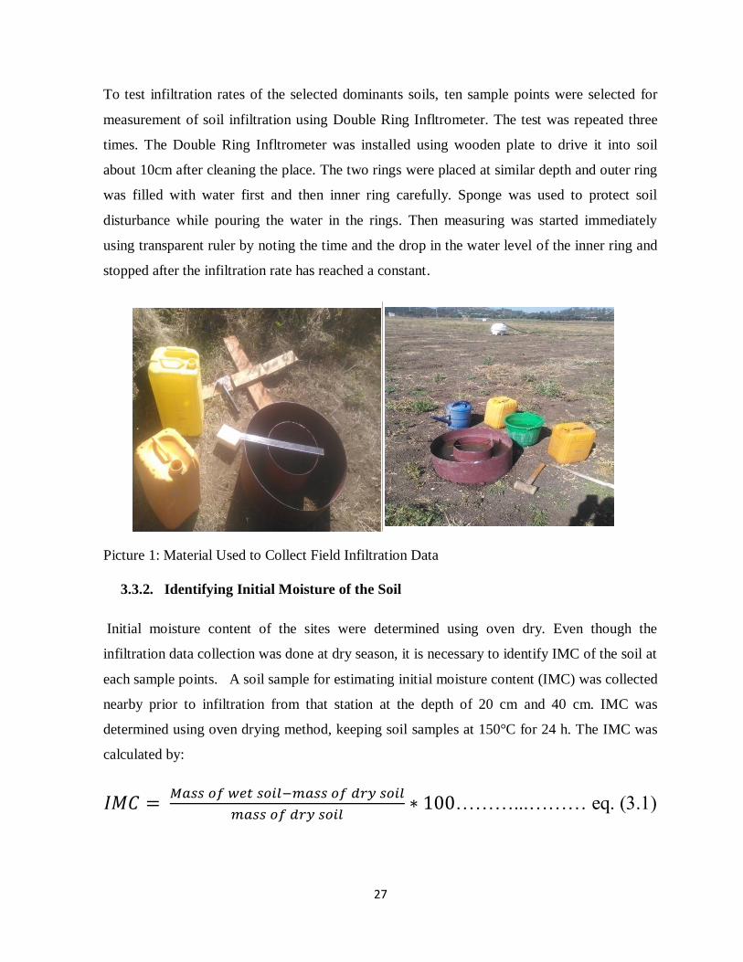
To test infiltration rates of the selected dominants soils, ten sample points were selected for

measurement of soil infiltration using Double Ring Infltrometer. The test was repeated three

times. The Double Ring Infltrometer was installed using wooden plate to drive it into soil

about 10cm after cleaning the place. The two rings were placed at similar depth and outer ring

was filled with water first and then inner ring carefully. Sponge was used to protect soil

disturbance while pouring the water in the rings. Then measuring was started immediately

using transparent ruler by noting the time and the drop in the water level of the inner ring and

stopped after the infiltration rate has reached a constant.

Picture 1: Material Used to Collect Field Infiltration Data

3.3.2. Identifying Initial Moisture of the Soil

Initial moisture content of the sites were determined using oven dry. Even though the

infiltration data collection was done at dry season, it is necessary to identify IMC of the soil at

each sample points. A soil sample for estimating initial moisture content (IMC) was collected

nearby prior to infiltration from that station at the depth of 20 cm and 40 cm. IMC was

determined using oven drying method, keeping soil samples at 150°C for 24 h. The IMC was

calculated by:

………...……… eq. (3.1)

28

3.3.3. Estimating Infiltration Parameters of Cambisols and Vertisols

To identify infiltration capacities of both Vertisol and Cambisols, field infiltration data was

collected from ASTU and Bishoftu Research Center. Four infiltration models, Horton, Philip,

Kostiakov and Green-Ampt were used. Using field infiltration data, the values of various

parameters of these models was determined. To determine these infiltration parameters, the

graphing method was used. This approach is stated by Subramanya (2008). Additionally,

Sreejani et al. (2017), Ibrahim et al. (2019), Abubakr and Byzedi (2012), Ayu et al. (2013),

Abdulkadir et al. (2011) were used graph approach to find infiltration parameters.

Accordingly, graph method used to determine infiltration parameters of the four infiltration

models is described below.

A. Horton’s Equation (1933): Horton expressed the decay of infiltration capacity with

time as an exponential decay given by

…………….…………………Eq. (3.2)

Where,

fp = infiltration capacity at any time t from the start of the rainfall.

f0= initial infiltration capacity at t = 0

fc = final steady state infiltration capacity occurring at t = tc. Also, fc is sometimes

known as constant rate or ultimate infiltration capacity

= Horton‟s decay coefficient which depends upon soil characteristics and Vegetation

cover.

By rearranging equation 1:

…………….……………..………………...…..….... Eq. (3.3)

Taking natural logarithm to both sides

……………………………………………………...Eq. (3.4)

Computing the values of the infiltration rates at different times and final steady-state

infiltration (fc), was plotted on graph, using excel sheet. So, the

values of fp and fc were identified from field infiltration rate data. Then arranging time and the

values of ( ) on the excel sheet and graphing it was used to find the value of

as intercept and k is taken as slope.

29

B. Philip’s Equation (1957) Philip‟s two term model relates Fp (t) as

…………………………………………....……………….Eq. (3.5)

Where

s = a function of soil suction potential and called as sorptivity.

K = Darcy‟s hydraulic Conductivity.

Fp = Cumulative infiltration capacity

To determine these infiltration parameters, graph approach was also used as described for

Horton Model.

⁄

⁄ …………………………………………………….……...…. Eq. (3.6)

Where: f = infiltration rate

From field observation data, infiltration rate data with its respect to time was arranged in excel

sheet and the time was arranged as t-1/2

. Then by plotting the graph of this infiltration rate with

this value of time t, the value of, S/2 and K were identified as slope and intercept respectively

from the graph as described earlier.

C. Kostiakov Equation (1932): it expresses cumulative infiltration capacity as

………………………….…………………………………….…..Eq. (3.7)

Where,

Fp is Cumulative infiltration capacity

a and b are local parameters with a > 0 and 0 < b< 1.

To determine a and b parameters, taking natural logarithm to both sides

:

…........................................................................................Eq. (3.8)

Different cumulative infiltration capacity at different time and lnt was arranged on excel and

then graph was used to find lna as intercept and b as slope.

D. Green – Ampt Equation (1911): Green and Ampt proposed a model for infiltration

capacity based on Darcy‟s law as

30

( (

))………………………………………………..……………Eq. (3.9)

Where

= Porosity of the soil.

= Capillary suction at the wetting front and

K = Darcy‟s Hydraulic Conductivity.

= infiltration capacity

= cumulative infiltration capacity

The above equation can be considered as,

(

)…………………………………………………………………Eq. (3.10)

Where m and n are Green – Ampt parameters of infiltration model

To determine these m and n parameters, the values of were plotted against

, using excel

sheet. Then the intercept and slope of the line are m and n respectively.

After the values of fo, fc and of Horton, S and K of Philip, a and b of Kostiakov and m and

n of Green Ampt infiltration models were collected from the graph, the models were used to

calculate infiltration capacity and infiltration rate of both Cambisols and Vertisols. Then the

models were compared using R2 and RMSE to select best fit model. The detail comparison

method was described below.

3.3.4. Comparing Performance of Different Infiltration Models

Using determined infiltration parameters, four infiltration models were compared with the

values of infiltration rates of field observed one and at any time t. The root mean square error

(RMSE), coefficient of determination (R2) and Nash-Sutcliffe (NS) were used for comparison.

Different scholars used different statistical tools to compare Infiltration Models. Ogbe et al.

(2011) used the RMSE and R2 to compare Kostiakov, modified Kostiakov, Philip and

Horton‟s Infiltration Models while Sreejani et al. (2017) used Correlation Coefficient and

Standard Error tools to compare Horton, Kostiakov, Philip and Green Ampt Infiltration

Models. On the other hand, David et al. (2018) used Correlation Coefficient, Standard Error

31

and coefficient of determination (R2) to compare Horton, Kostiakov and Green Ampt

Infiltration Models. And Abubakr and Byzedi (2012) also used coefficient of determination

and variation to compare Kostiakov, Kostiakov_Lowies, Philip and SCS.

The goodness of fit of each model was tested by both the R2 and the RMSE to evaluate how

closely each model describes the measured infiltration. The R2 values indicate the degree to

which data variations are explained by each model, while RMSE shows the amount of

divergence of the model values from the observed values. Therefore, a high R2 which is close

to 1 and a low RMSE value which is close to 0 both indicate a good agreement between the

predicted and observed infiltration curves.

The RMSE provides a measure of deviation of predicted values from measured data and has

frequently been used as means of evaluating the accuracy of hydrologic models. The RMSE is

calculated as follows:

√(∑

)

…………………….………………………………..Eq. (3.11)

Where:

Pi = Predicted Value

Oi = Measured/observed value

n = number of measurements

Predicted value of infiltration rate will be plotted versus observed values and coefficient of

determination (R2) will be calculated for each model according to the equation

………………………….………………………….………………Eq. (3.12)

Where,

SSE = Explained Sum of Square

SST = Total Sum of Square

The R2

values indicate the degree to which data variations are explained by each model.

RMSE shows the amount of divergence of the model values from the observed values.

Nash-Sutcliffe is the most frequently used to compare hydrological parameters. The equation

of Nash-Sutcliffe is:

32

∑ (

)

∑

………………………………………………….. Eq. (3.13)

Where,

n = number of observed data point

yti = observation values

ytim = model values

= average value of observation

3.3.5. Setting Equation for Both Cambisols and Vertisols

Infiltration rate and infiltration capacity of both Cambisols and Vertisols was collected from

field. These data were analyzed using Excel sheet to quantify infiltration parameters of the

four infiltration models, those selected for the analysis. Then using the values of different

infiltration parameters of these infiltration models, Horton, Kostiakov, Philip and Green Ampt,

the equations of these models were set.

The determined infiltration parameters of all ten sample points were inserted in infiltration

model equations to develop equation for the sites. Finally, from estimated infiltration

parameters, infiltration model for both Cambisols and Vertisols was developed by substituting

it into the model equation to obtain the specific infiltration equations for the soils of the study area.

These equations were also tested for accuracy by comparing cumulative infiltration capacity that

was measured at field and cumulative infiltration capacity the model estimate.

3.3.6. Check for Accuracy of Model Infiltration Equations

The developed infiltration models for each point was checked for validity by relating cumulative

infiltration rate of the soil that was measured at field and the cumulative infiltration value that is

calculated from the model. Integration of the developed infiltration model was used to compare

with cumulative infiltration rate of the model. The model was integrated by the time from the

infiltration start, zero, to the time required to get constant infiltration rate. And the model which

estimate the value of cumulative infiltration that is similar or nearly similar with field cumulative

infiltration was recommended as valid model for the site.

33

This method was used by different scholars. Arshad et al., (2015) investigated the effect of

tillage intensity to the water transmission behavior for sandy loam soil in terms of infiltration

rates and cumulative infiltration and its validation with different infiltration models. The

scholar used to compare observed cumulative infiltration and model cumulative infiltration for

model validation. Standard Deviation, Standard Error and Coefficient of determination was

used for comparison. Finally, the scholar concluded that Horton infiltration model is accurate

model for the site.

The accuracy of the different equations for predicting the cumulative infiltration were

evaluated by comparing the observed values of measurement on the field and the predicted

values based on the fitted equation. The cumulative infiltration values predicted using the

infiltration models and those measured were plotted against each other and fitted with a linear

equation with zero intercept to verify the validity of each prediction. The slope of the line of

best fit and its coefficient of determination (R2) for each model. To check the discrepancies

between the predicted and the measured values, paired t-test and Root Mean Square Error

(RMSE) were used. Considering the four infiltration models evaluated, the Horton‟s models

gave best fit to the measured cumulative infiltration, although the other models provided good

overall agreement with the field measured cumulative infiltration depths (Ogbe et al., 2011)

Based on this, accuracy of the models were tested by comparing field cumulative infiltration

capacity data and the model cumulative infiltration capacity. The infiltration equations of the

four infiltration models were integrated to calculate infiltration capacity using these models.

Then, the values of cumulative infiltration capacity were compared with values of the field

cumulative infiltration capacity with respect to time. Standard Error, Coefficient of

determination, percentage of error and Nash-Sutcliffe were used for comparison

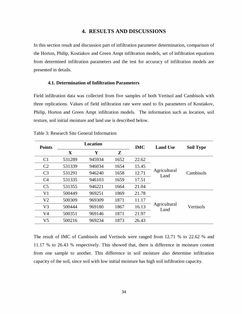
34

4. RESULTS AND DISCUSSIONS

In this section result and discussion part of infiltration parameter determination, comparison of

the Horton, Philip, Kostiakov and Green Ampt infiltration models, set of infiltration equations

from determined infiltration parameters and the test for accuracy of infiltration models are

presented in details.

4.1. Determination of Infiltration Parameters

Field infiltration data was collected from five samples of both Vertisol and Cambisols with

three replications. Values of field infiltration rate were used to fix parameters of Kostiakov,

Philip, Horton and Green Ampt infiltration models. The information such as location, soil

texture, soil initial moisture and land use is described below.

Table 3: Research Site General Information

Points Location

IMC Land Use Soil Type

X Y Z

C1 531289 945934 1652 22.62

Agricultural

Land Cambisols

C2 531339 946034 1654 15.45

C3 531291 946240 1658 12.71

C4 531335 946103 1659 17.51

C5 531355 946221 1664 21.04

V1 500449 969251 1869 21.78

Agricultural

Land Vertisols

V2 500309 969309 1871 11.17

V3 500444 969180 1867 16.13

V4 500351 969146 1871 21.97

V5 500216 969234 1873 26.43

The result of IMC of Cambisols and Vertisols were ranged from 12.71 % to 22.62 % and

11.17 % to 26.43 % respectively. This showed that, there is difference in moisture content

from one sample to another. This difference in soil moisture also determine infiltration

capacity of the soil, since soil with low initial moisture has high soil infiltration capacity.

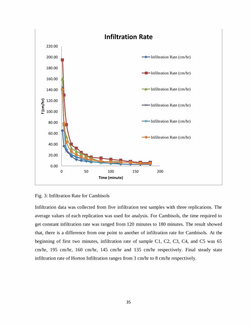
35

Fig. 3: Infiltration Rate for Cambisols

Infiltration data was collected from five infiltration test samples with three replications. The

average values of each replication was used for analysis. For Cambisols, the time required to

get constant infiltration rate was ranged from 120 minutes to 180 minutes. The result showed

that, there is a difference from one point to another of infiltration rate for Cambisols. At the

beginning of first two minutes, infiltration rate of sample C1, C2, C3, C4, and C5 was 65

cm/hr, 195 cm/hr, 160 cm/hr, 145 cm/hr and 135 cm/hr respectively. Final steady state

infiltration rate of Horton Infiltration ranges from 3 cm/hr to 8 cm/hr respectively.

0.00

20.00

40.00

60.00

80.00

100.00

120.00

140.00

160.00

180.00

200.00

220.00

0 50 100 150 200

f (c

m/h

r)

Time (minute)

Infiltration Rate

Infiltration Rate (cm/hr)






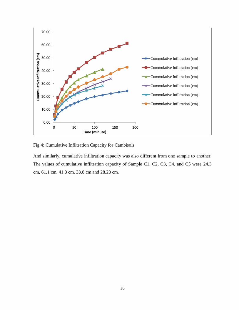
36

Fig 4: Cumulative Infiltration Capacity for Cambisols

And similarly, cumulative infiltration capacity was also different from one sample to another.

The values of cumulative infiltration capacity of Sample C1, C2, C3, C4, and C5 were 24.3

cm, 61.1 cm, 41.3 cm, 33.8 cm and 28.23 cm.

0.00

10.00

20.00

30.00

40.00

50.00

60.00

70.00

0 50 100 150 200

Cu

mm

ula

tive

Infi

ltra

tio

n (c

m)

Time (minute)

Cummulative Infiltration (cm)






37

Fig. 5: Infiltration Rate for Vertisol

Similarly, soil infiltration rate and cumulative infiltration of Vertisols were collected from five

different samples with three replications from agricultural land of Bishoftu Research Center.

The result of this site also showed that, there was different values of infiltration rate from one

sample to another. The values of infiltration rate for beginning of first two minutes were 12

cm/hr, 15 cm/hr, 68 cm/hr, 77 cm/hr and 42 cm/hr for sample V1, V2, V3, V4, and V5

respectively. Final steady state infiltration rate of Horton Infiltration ranges from 3 cm/hr to 8

cm/hr respectively. Similarly, there was different values of constant infiltration rate for each

sample. Accordingly, there were constant infiltration rate values of V1, V2, V3, V4, and V5 as

0.73 cm/hr, 0.3 cm/hr, 1.33 cm/hr, 1.87 cm/hr, and 1.73 cm/hr.

0.00

10.00

20.00

30.00

40.00

50.00

60.00

70.00

80.00

90.00

0 50 100 150 200 250

CI

(cm

)

Time (minute)

Cumulative infiltration Capacity






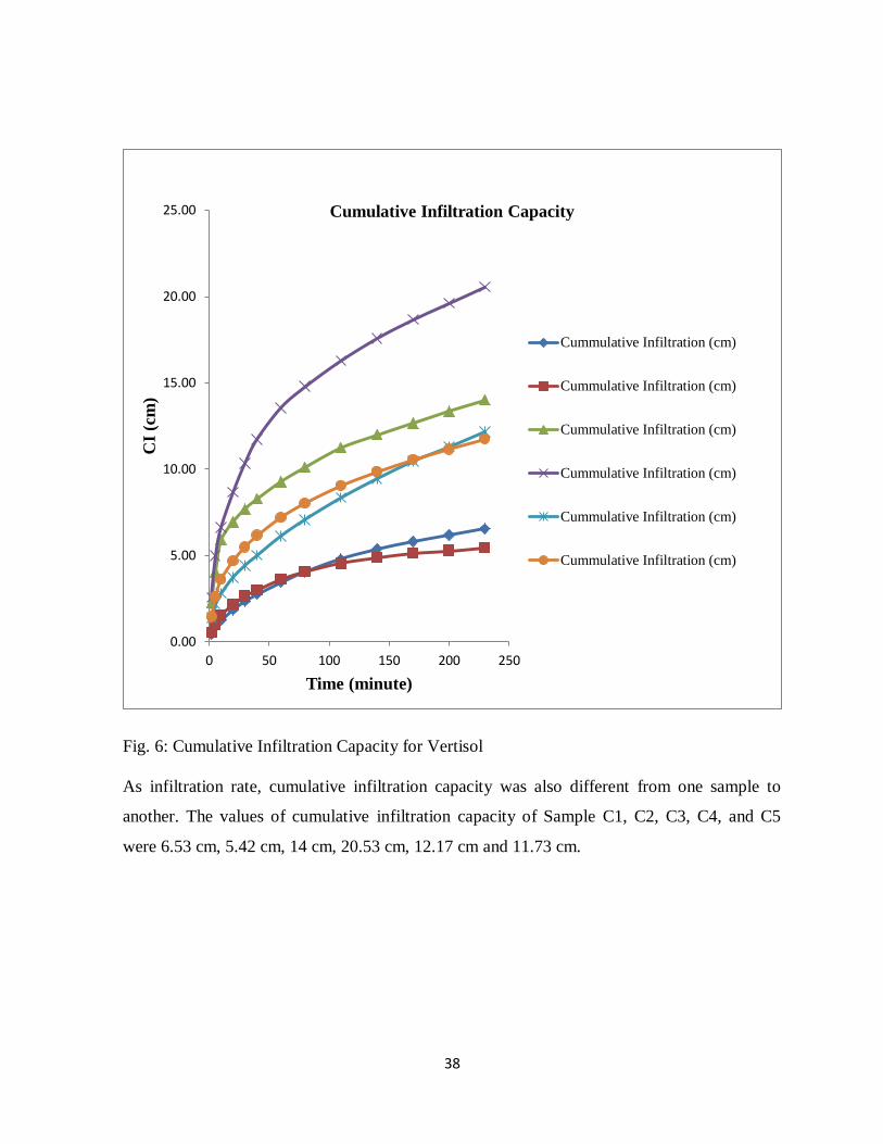
38

Fig. 6: Cumulative Infiltration Capacity for Vertisol

As infiltration rate, cumulative infiltration capacity was also different from one sample to

another. The values of cumulative infiltration capacity of Sample C1, C2, C3, C4, and C5

were 6.53 cm, 5.42 cm, 14 cm, 20.53 cm, 12.17 cm and 11.73 cm.

0.00

5.00

10.00

15.00

20.00

25.00

0 50 100 150 200 250

CI

(cm

)

Time (minute)

Cumulative Infiltration Capacity







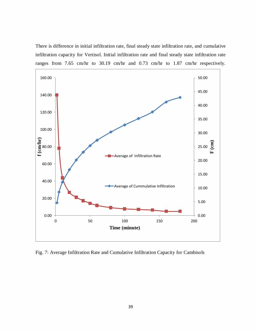
39

There is difference in initial infiltration rate, final steady state infiltration rate, and cumulative

infiltration capacity for Vertisol. Initial infiltration rate and final steady state infiltration rate

ranges from 7.65 cm/hr to 30.19 cm/hr and 0.73 cm/hr to 1.87 cm/hr respectively.

Fig. 7: Average Infiltration Rate and Cumulative Infiltration Capacity for Cambisols

0.00

5.00

10.00

15.00

20.00

25.00

30.00

35.00

40.00

45.00

50.00

0.00

20.00

40.00

60.00

80.00

100.00

120.00

140.00

160.00

0 50 100 150 200

F (

cm)

f (c

m/h

r)

Time (minute)

Average of Infiltration Rate

Average of Cummulative Infiltration

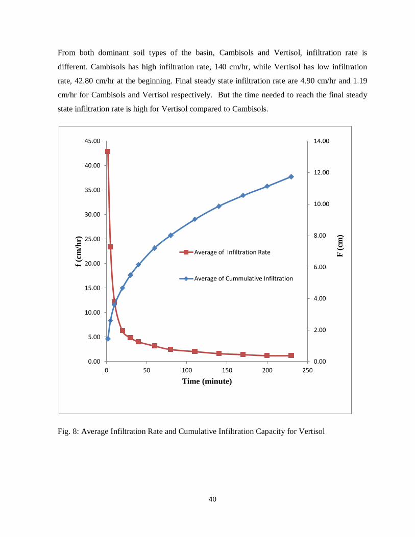
40

From both dominant soil types of the basin, Cambisols and Vertisol, infiltration rate is

different. Cambisols has high infiltration rate, 140 cm/hr, while Vertisol has low infiltration

rate, 42.80 cm/hr at the beginning. Final steady state infiltration rate are 4.90 cm/hr and 1.19

cm/hr for Cambisols and Vertisol respectively. But the time needed to reach the final steady

state infiltration rate is high for Vertisol compared to Cambisols.

Fig. 8: Average Infiltration Rate and Cumulative Infiltration Capacity for Vertisol

0.00

2.00

4.00

6.00

8.00

10.00

12.00

14.00

0.00

5.00

10.00

15.00

20.00

25.00

30.00

35.00

40.00

45.00

0 50 100 150 200 250

F (

cm)

f (c

m/h

r)

Time (minute)

Average of Infiltration Rate

Average of Cummulative Infiltration

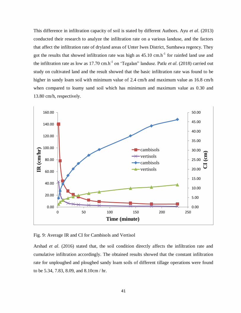
41

This difference in infiltration capacity of soil is stated by different Authors. Ayu et al. (2013)

conducted their research to analyze the infiltration rate on a various landuse, and the factors

that affect the infiltration rate of dryland areas of Unter Iwes District, Sumbawa regency. They

got the results that showed infiltration rate was high as 45.10 cm.h-1

for rainfed land use and

the infiltration rate as low as 17.70 cm.h-1

on „Tegalan” landuse. Patle et al. (2018) carried out

study on cultivated land and the result showed that the basic infiltration rate was found to be

higher in sandy loam soil with minimum value of 2.4 cm/h and maximum value as 16.8 cm/h

when compared to loamy sand soil which has minimum and maximum value as 0.30 and

13.80 cm/h, respectively.

Fig. 9: Average IR and CI for Cambisols and Vertisol

Arshad et al. (2016) stated that, the soil condition directly affects the infiltration rate and

cumulative infiltration accordingly. The obtained results showed that the constant infiltration

rate for unploughed and ploughed sandy loam soils of different tillage operations were found

to be 5.34, 7.83, 8.09, and 8.10cm / hr.

0.00

5.00

10.00

15.00

20.00

25.00

30.00

35.00

40.00

45.00

50.00

0.00

20.00

40.00

60.00

80.00

100.00

120.00

140.00

160.00

0 50 100 150 200 250

CI

(cm

)

IR (

cm

/hr)

Time (minute)

cambisols

vertisols

cambisols

vertisols

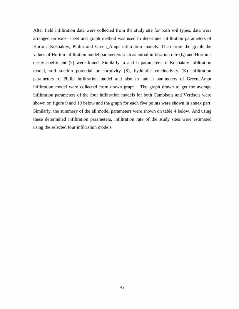
42

After field infiltration data were collected from the study site for both soil types, data were

arranged on excel sheet and graph method was used to determine infiltration parameters of

Horton, Kostiakov, Philip and Green_Ampt infiltration models. Then from the graph the

values of Horton infiltration model parameters such as initial infiltration rate (f0) and Horton‟s

decay coefficient (k) were found. Similarly, a and b parameters of Kostiakov infiltration

model, soil suction potential or sorptivity (S), hydraulic conductivity (K) infiltration

parameters of Philip infiltration model and also m and n parameters of Green_Ampt

infiltration model were collected from drawn graph. The graph drawn to get the average

infiltration parameters of the four infiltration models for both Cambisols and Vertisols were

shown on figure 9 and 10 below and the graph for each five points were shown in annex part.

Similarly, the summery of the all model parameters were shown on table 4 below. And using

these determined infiltration parameters, infiltration rate of the study sites were estimated

using the selected four infiltration models.

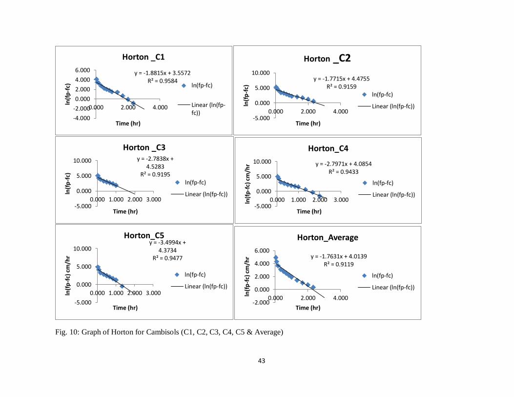
43

Fig. 10: Graph of Horton for Cambisols (C1, C2, C3, C4, C5 & Average)

y = -1.8815x + 3.5572 R² = 0.9584

-4.000

-2.000

0.000

2.000

4.000

6.000

0.000 2.000 4.000

ln(f

p-f

c)

Time (hr)

Horton _C1

ln(fp-fc)

Linear (ln(fp-fc))

y = -1.7715x + 4.4755 R² = 0.9159

-5.000

0.000

5.000

10.000

0.000 2.000 4.000

ln(f

p-f

c)

Time (hr)

Horton _C2

ln(fp-fc)

Linear (ln(fp-fc))

y = -2.7838x + 4.5283

R² = 0.9195

-5.000

0.000

5.000

10.000

0.000 1.000 2.000 3.000

ln(f

p-f

c)

Time (hr)

Horton _C3

ln(fp-fc)

Linear (ln(fp-fc))

y = -2.7971x + 4.0854 R² = 0.9433

-5.000

0.000

5.000

10.000

0.000 1.000 2.000 3.000ln(f

p-f

c) c

m/h

r

Time (hr)

Horton_C4

ln(fp-fc)

Linear (ln(fp-fc))

y = -3.4994x + 4.3734

R² = 0.9477

-5.000

0.000

5.000

10.000

0.000 1.000 2.000 3.000ln(f

p-f

c) c

m/h

r

Time (hr)

Horton_C5

ln(fp-fc)

Linear (ln(fp-fc))

y = -1.7631x + 4.0139 R² = 0.9119

-2.000

0.000

2.000

4.000

6.000

0.000 2.000 4.000

ln(f

p-f

c) c

m/h

r

Time (hr)

Horton_Average

ln(fp-fc)

Linear (ln(fp-fc))

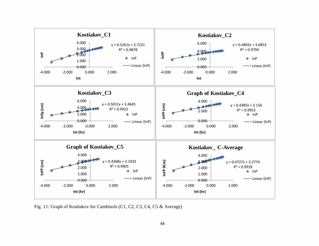
44

Fig. 11: Graph of Kostiakov for Cambisols (C1, C2, C3, C4, C5 & Average)

y = 0.5261x + 2.7231 R² = 0.9878

0.000

1.000

2.000

3.000

4.000

-4.000 -2.000 0.000 2.000

lnP

lnt

Kostiakov_C1

lnP

Linear (lnP)

y = 0.4802x + 3.6853 R² = 0.9794

0.000

2.000

4.000

6.000

-4.000 -2.000 0.000 2.000

lnFP

lnt

Kostiakov_C2

lnP

Linear (lnP)

y = 0.5011x + 3.4645 R² = 0.9922

0.000

2.000

4.000

6.000

-4.000 -2.000 0.000 2.000

lnFp

(cm

)

lnt (hr)

Kostiakov_C3

lnP

Linear (lnP)

y = 0.4385x + 3.156 R² = 0.9953

0.000

2.000

4.000

-4.000 -2.000 0.000 2.000

lnFP

(cm

)

lnt (hr)

Graph of Kostiakov_C4

lnP

Linear (lnP)

y = 0.4368x + 3.1033 R² = 0.9905

0.000

1.000

2.000

3.000

4.000

-4.000 -2.000 0.000 2.000

lnFP

(cm

)

lnt (hr)

Graph of Kostiakov_C5

lnP

Linear (lnP)

y = 0.4727x + 3.2774 R² = 0.9918

0.000

1.000

2.000

3.000

4.000

-4.000 -2.000 0.000 2.000

lnFP

9C

m)

lnt (hr)

Kostiakov_ C-Average

lnP

Linear (lnP)

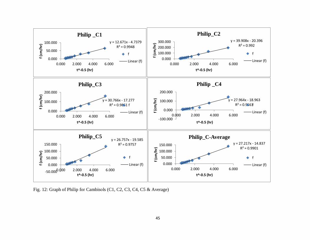
45

Fig. 12: Graph of Philip for Cambisols (C1, C2, C3, C4, C5 & Average)

y = 12.671x - 4.7379 R² = 0.9948

0.000

50.000

100.000

0.000 2.000 4.000 6.000

f (c

m/h

r)

t^-0.5 (hr)

Philip _C1

f

Linear (f)

y = 39.908x - 20.396 R² = 0.992

0.000

100.000

200.000

300.000

0.000 2.000 4.000 6.000

f (c

m/h

r)

t^-0.5 (hr)

Philip_C2

f

Linear (f)

y = 30.766x - 17.277 R² = 0.9861

0.000

100.000

200.000

0.000 2.000 4.000 6.000

f (c

m/h

r)

t^-0.5 (hr)

Philip_C3

f

Linear (f)

y = 27.964x - 18.963 R² = 0.9563

-100.000

0.000

100.000

200.000

0.000 2.000 4.000 6.000

f (c

m/h

r)

t^-0.5 (hr)

Philip _C4

f

Linear (f)

y = 26.757x - 19.585 R² = 0.9757

-50.000

0.000

50.000

100.000

150.000

0.000 2.000 4.000 6.000

f (c

m/h

r)

t^-0.5 (hr)

Philip_C5

f

Linear (f)

y = 27.217x - 14.837 R² = 0.9901

0.000

50.000

100.000

150.000

0.000 2.000 4.000 6.000

f (c

m/h

r)

t^-0.5 (hr)

Philip_C-Average

f

Linear (f)

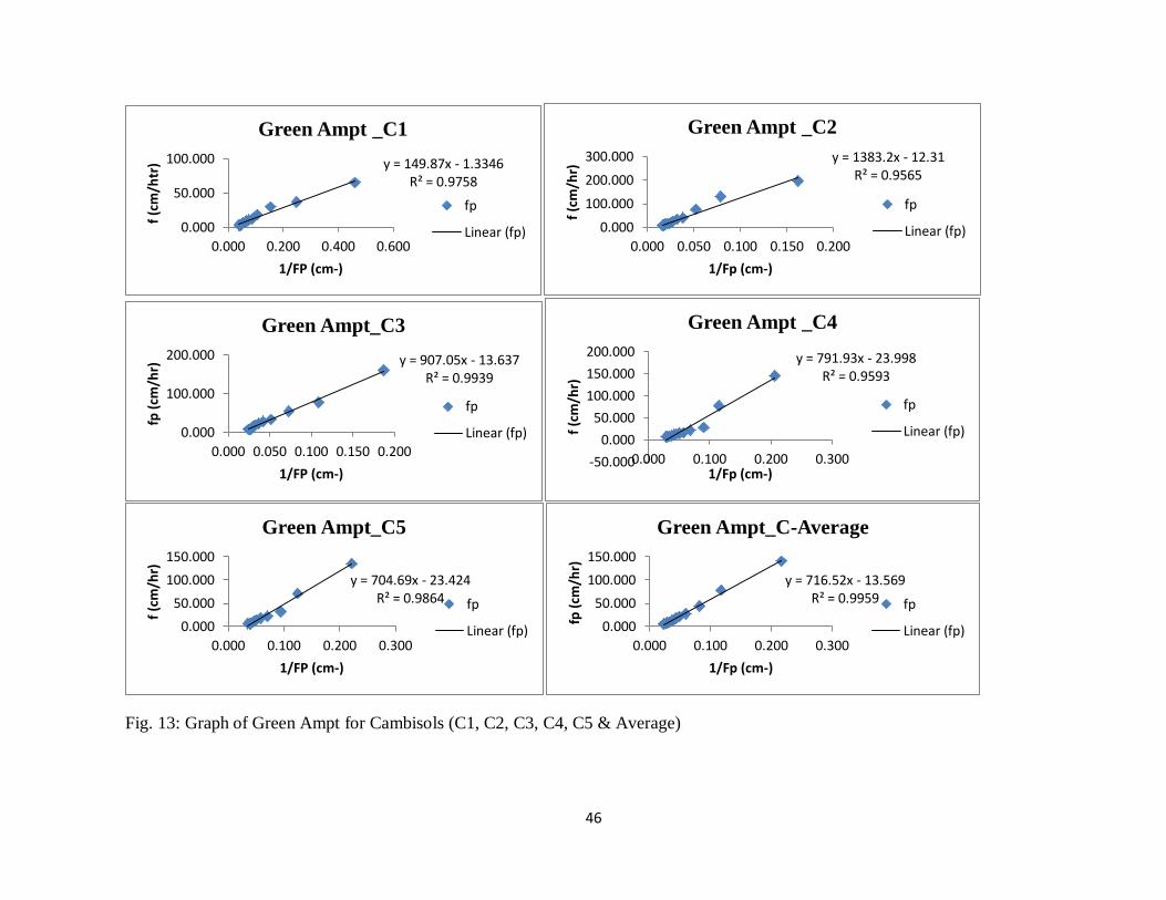
46

Fig. 13: Graph of Green Ampt for Cambisols (C1, C2, C3, C4, C5 & Average)

y = 149.87x - 1.3346 R² = 0.9758

0.000

50.000

100.000

0.000 0.200 0.400 0.600

f (c

m/h

tr)

1/FP (cm-)

Green Ampt _C1

fp

Linear (fp)

y = 1383.2x - 12.31 R² = 0.9565

0.000

100.000

200.000

300.000

0.000 0.050 0.100 0.150 0.200

f (c

m/h

r)

1/Fp (cm-)

Green Ampt _C2

fp

Linear (fp)

y = 907.05x - 13.637 R² = 0.9939

0.000

100.000

200.000

0.000 0.050 0.100 0.150 0.200

fp (

cm/h

r)

1/FP (cm-)

Green Ampt_C3

fp

Linear (fp)

y = 791.93x - 23.998 R² = 0.9593

-50.000

0.000

50.000

100.000

150.000

200.000

0.000 0.100 0.200 0.300

f (c

m/h

r)

1/Fp (cm-)

Green Ampt _C4

fp

Linear (fp)

y = 704.69x - 23.424 R² = 0.9864

0.000

50.000

100.000

150.000

0.000 0.100 0.200 0.300

f (c

m/h

r)

1/FP (cm-)

Green Ampt_C5

fp

Linear (fp)

y = 716.52x - 13.569 R² = 0.9959

0.000

50.000

100.000

150.000

0.000 0.100 0.200 0.300

fp (

cm/h

r)

1/Fp (cm-)

Green Ampt_C-Average

fp

Linear (fp)

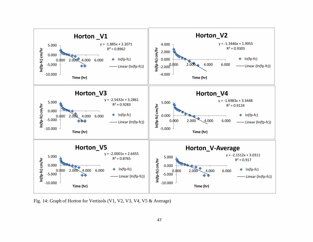
47

Fig. 14: Graph of Horton for Vertisols (V1, V2, V3, V4, V5 & Average)

y = -1.885x + 2.2071 R² = 0.8962

-10.000

-5.000

0.000

5.000

0.000 2.000 4.000 6.000

ln(f

p-f

c) c

m/h

r

Time (hr)

Horton _V1

ln(fp-fc)

Linear (ln(fp-fc))

y = -1.3446x + 1.9955 R² = 0.9303

-4.000

-2.000

0.000

2.000

4.000

0.000 2.000 4.000 6.000

ln(f

p-f

c) c

m/h

r

Time (hr)

Horton_V2

ln(fp-fc)

Linear (ln(fp-fc))

y = -2.5432x + 3.2861 R² = 0.9283

-10.000

-5.000

0.000

5.000

0.000 2.000 4.000 6.000

ln(f

p-f

c) c

m/h

r

Time (hr)

Horton_V3

ln(fp-fc)

Linear (ln(fp-fc))

y = -1.6983x + 3.3448 R² = 0.9124

-5.000

0.000

5.000

0.000 2.000 4.000 6.000

ln(f

p-f

c) c

m/h

r

Time (hr)

Horton_V4

ln(fp-fc)

Linear (ln(fp-fc))

y = -2.0001x + 2.6455 R² = 0.8765

-10.000

-5.000

0.000

5.000

0.000 2.000 4.000 6.000

ln(f

p-f

c) c

m/h

r

Time (hr)

Horton_V5

ln(fp-fc)

Linear (ln(fp-fc))

y = -2.1512x + 3.0311 R² = 0.917

-10.000

-5.000

0.000

5.000

0.000 2.000 4.000 6.000

ln(f

p-f

c) c

m/h

r

Time (hr)

Horton_V-Average

ln(fp-fc)

Linear (ln(fp-fc))

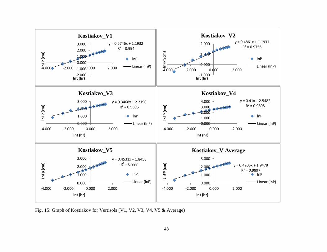
48

Fig. 15: Graph of Kostiakov for Vertisols (V1, V2, V3, V4, V5 & Average)

y = 0.5746x + 1.1932 R² = 0.994

-2.000

-1.000

0.000

1.000

2.000

3.000

-4.000 -2.000 0.000 2.000lnFP

(cm

)

lnt (hr)

Kostiakov_V1

lnP

Linear (lnP)

y = 0.4861x + 1.1931 R² = 0.9756

-1.000

0.000

1.000

2.000

-4.000 -2.000 0.000 2.000

lnFP

9cm

)

lnt (hr)

Kostiakov_V2

lnP

Linear (lnP)

y = 0.3468x + 2.2196 R² = 0.9696

0.000

1.000

2.000

3.000

-4.000 -2.000 0.000 2.000

lnFP

(cm

)

lnt (hr)

Kostiakvo_V3

lnP

Linear (lnP)

y = 0.41x + 2.5482 R² = 0.9808

0.000

1.000

2.000

3.000

4.000

-4.000 -2.000 0.000 2.000

lnFP

(cm

)

lnt (hr)

Kostiakov_V4

lnP

Linear (lnP)

y = 0.4531x + 1.8458 R² = 0.997

0.000

1.000

2.000

3.000

-4.000 -2.000 0.000 2.000

LnFp

(cm

)

lnt (hr)

Kostiakov_V5

lnP

Linear (lnP)

y = 0.4205x + 1.9479 R² = 0.9897

0.000

1.000

2.000

3.000

-4.000 -2.000 0.000 2.000

LnFP

(cm

)

lnt (hr)

Kostiakov_V-Average

lnP

Linear (lnP)

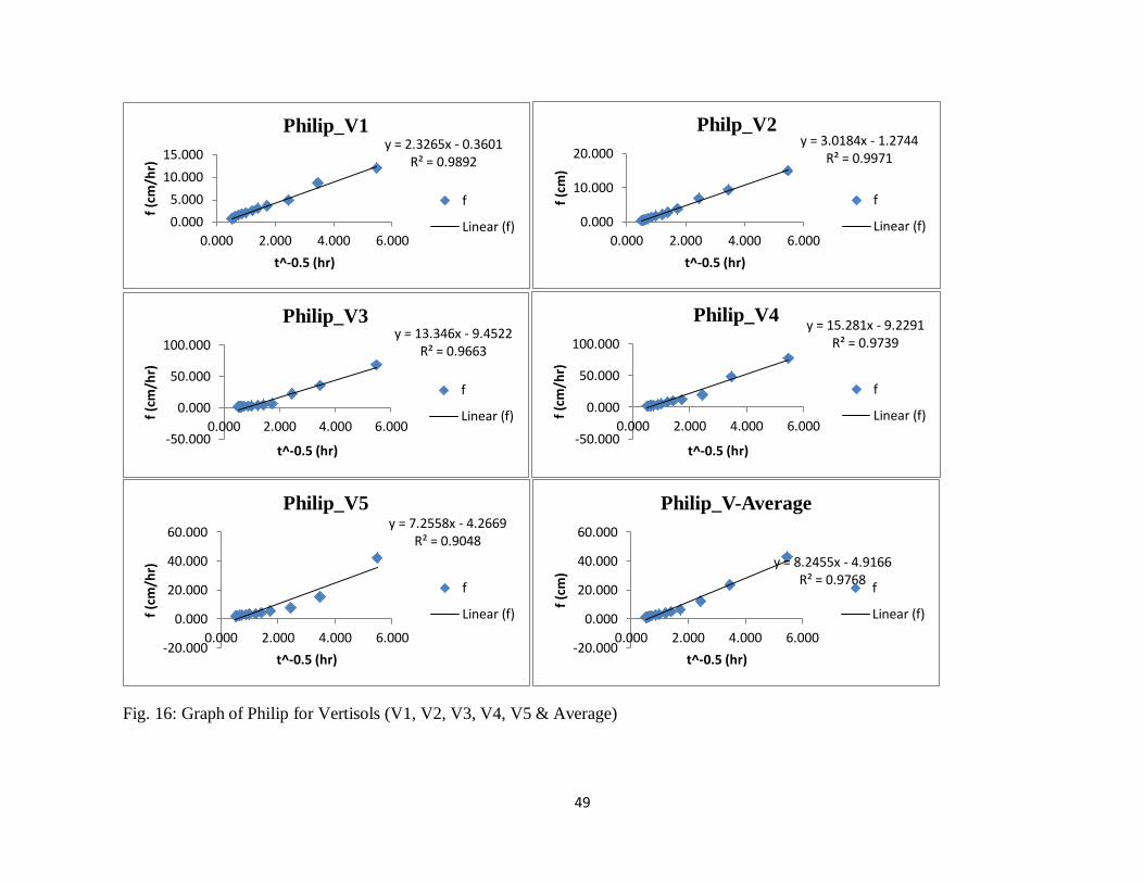
49

Fig. 16: Graph of Philip for Vertisols (V1, V2, V3, V4, V5 & Average)

y = 2.3265x - 0.3601 R² = 0.9892

0.000

5.000

10.000

15.000

0.000 2.000 4.000 6.000

f (c

m/h

r)

t^-0.5 (hr)

Philip_V1

f

Linear (f)

y = 3.0184x - 1.2744 R² = 0.9971

0.000

10.000

20.000

0.000 2.000 4.000 6.000

f (c

m)

t^-0.5 (hr)

Philp_V2

f

Linear (f)

y = 13.346x - 9.4522 R² = 0.9663

-50.000

0.000

50.000

100.000

0.000 2.000 4.000 6.000

f (c

m/h

r)

t^-0.5 (hr)

Philip_V3

f

Linear (f)

y = 15.281x - 9.2291 R² = 0.9739

-50.000

0.000

50.000

100.000

0.000 2.000 4.000 6.000

f (c

m/h

r)

t^-0.5 (hr)

Philip_V4

f

Linear (f)

y = 7.2558x - 4.2669 R² = 0.9048

-20.000

0.000

20.000

40.000

60.000

0.000 2.000 4.000 6.000

f (c

m/h

r)

t^-0.5 (hr)

Philip_V5

f

Linear (f)

y = 8.2455x - 4.9166 R² = 0.9768

-20.000

0.000

20.000

40.000

60.000

0.000 2.000 4.000 6.000

f (c

m)

t^-0.5 (hr)

Philip_V-Average

f

Linear (f)

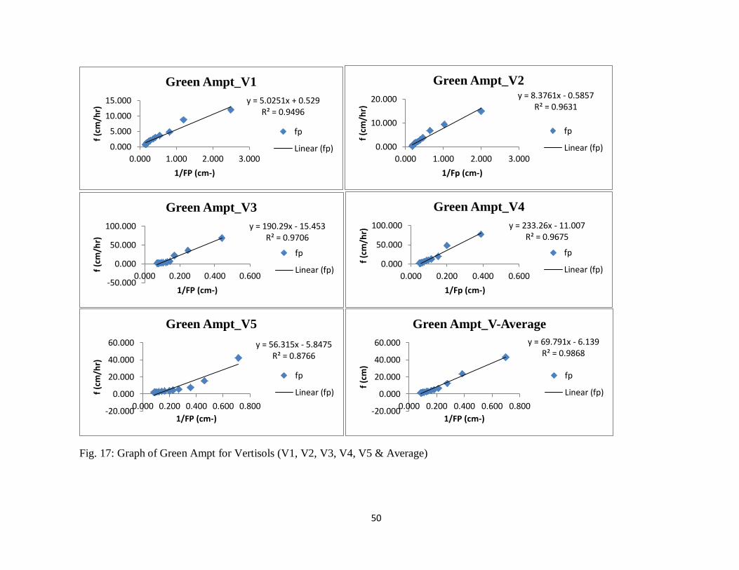
50

Fig. 17: Graph of Green Ampt for Vertisols (V1, V2, V3, V4, V5 & Average)

y = 5.0251x + 0.529 R² = 0.9496

0.000

5.000

10.000

15.000

0.000 1.000 2.000 3.000

f (c

m/h

r)

1/FP (cm-)

Green Ampt_V1

fp

Linear (fp)

y = 8.3761x - 0.5857 R² = 0.9631

0.000

10.000

20.000

0.000 1.000 2.000 3.000

f (c

m/h

r)

1/Fp (cm-)

Green Ampt_V2

fp

Linear (fp)

y = 190.29x - 15.453 R² = 0.9706

-50.000

0.000

50.000

100.000

0.000 0.200 0.400 0.600

f (c

m/h

r)

1/FP (cm-)

Green Ampt_V3

fp

Linear (fp)

y = 233.26x - 11.007 R² = 0.9675

0.000

50.000

100.000

0.000 0.200 0.400 0.600

f (c

m/h

r)

1/Fp (cm-)

Green Ampt_V4

fp

Linear (fp)

y = 56.315x - 5.8475 R² = 0.8766

-20.000

0.000

20.000

40.000

60.000

0.000 0.200 0.400 0.600 0.800

f (c

m/h

r)

1/FP (cm-)

Green Ampt_V5

fp

Linear (fp)

y = 69.791x - 6.139 R² = 0.9868

-20.000

0.000

20.000

40.000

60.000

0.000 0.200 0.400 0.600 0.800

f (c

m)

1/FP (cm-)

Green Ampt_V-Average

fp

Linear (fp)

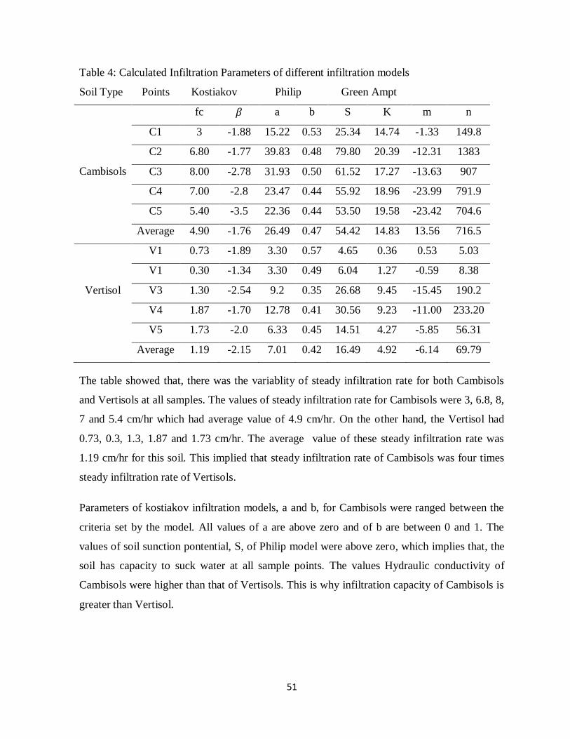
51

Table 4: Calculated Infiltration Parameters of different infiltration models

Soil Type Points Kostiakov Philip Green Ampt

Cambisols

fc a b S K m n

C1 3 -1.88 15.22 0.53 25.34 14.74 -1.33 149.8

C2 6.80 -1.77 39.83 0.48 79.80 20.39 -12.31 1383

C3 8.00 -2.78 31.93 0.50 61.52 17.27 -13.63 907

C4 7.00 -2.8 23.47 0.44 55.92 18.96 -23.99 791.9

C5 5.40 -3.5 22.36 0.44 53.50 19.58 -23.42 704.6

Average 4.90 -1.76 26.49 0.47 54.42 14.83 13.56 716.5

Vertisol

V1 0.73 -1.89 3.30 0.57 4.65 0.36 0.53 5.03

V1 0.30 -1.34 3.30 0.49 6.04 1.27 -0.59 8.38

V3 1.30 -2.54 9.2 0.35 26.68 9.45 -15.45 190.2

V4 1.87 -1.70 12.78 0.41 30.56 9.23 -11.00 233.20

V5 1.73 -2.0 6.33 0.45 14.51 4.27 -5.85 56.31

Average 1.19 -2.15 7.01 0.42 16.49 4.92 -6.14 69.79

The table showed that, there was the variablity of steady infiltration rate for both Cambisols

and Vertisols at all samples. The values of steady infiltration rate for Cambisols were 3, 6.8, 8,

7 and 5.4 cm/hr which had average value of 4.9 cm/hr. On the other hand, the Vertisol had

0.73, 0.3, 1.3, 1.87 and 1.73 cm/hr. The average value of these steady infiltration rate was

1.19 cm/hr for this soil. This implied that steady infiltration rate of Cambisols was four times

steady infiltration rate of Vertisols.

Parameters of kostiakov infiltration models, a and b, for Cambisols were ranged between the

criteria set by the model. All values of a are above zero and of b are between 0 and 1. The

values of soil sunction pontential, S, of Philip model were above zero, which implies that, the

soil has capacity to suck water at all sample points. The values Hydraulic conductivity of

Cambisols were higher than that of Vertisols. This is why infiltration capacity of Cambisols is

greater than Vertisol.

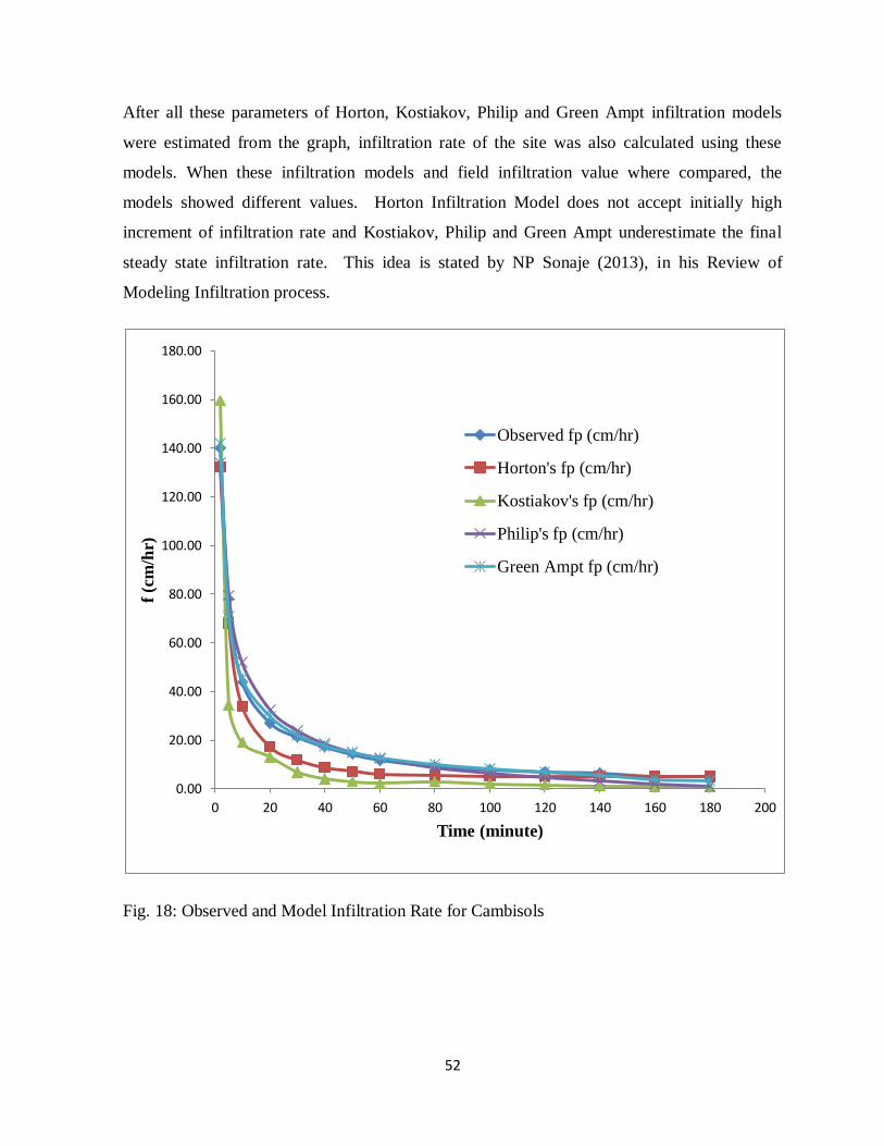
52

After all these parameters of Horton, Kostiakov, Philip and Green Ampt infiltration models

were estimated from the graph, infiltration rate of the site was also calculated using these

models. When these infiltration models and field infiltration value where compared, the

models showed different values. Horton Infiltration Model does not accept initially high

increment of infiltration rate and Kostiakov, Philip and Green Ampt underestimate the final

steady state infiltration rate. This idea is stated by NP Sonaje (2013), in his Review of

Modeling Infiltration process.

Fig. 18: Observed and Model Infiltration Rate for Cambisols

0.00

20.00

40.00

60.00

80.00

100.00

120.00

140.00

160.00

180.00

0 20 40 60 80 100 120 140 160 180 200

f (c

m/h

r)

Time (minute)

Observed fp (cm/hr)

Horton's fp (cm/hr)

Kostiakov's fp (cm/hr)

Philip's fp (cm/hr)

Green Ampt fp (cm/hr)

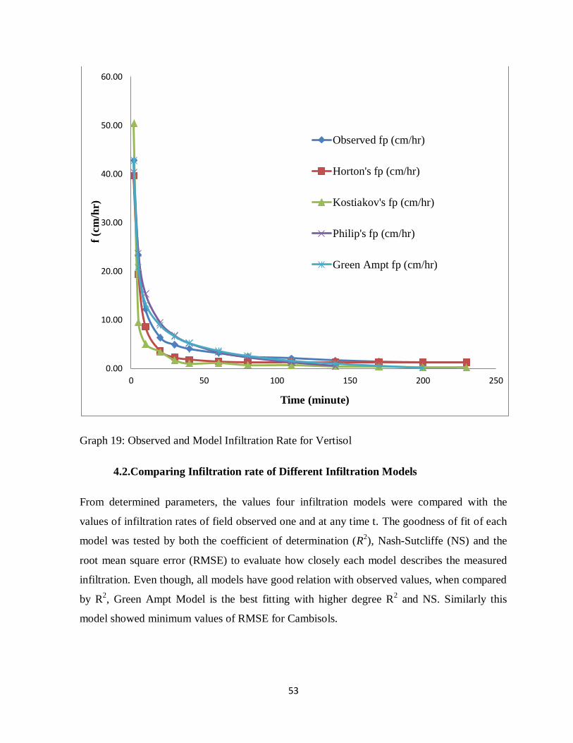
53

Graph 19: Observed and Model Infiltration Rate for Vertisol

4.2.Comparing Infiltration rate of Different Infiltration Models

From determined parameters, the values four infiltration models were compared with the

values of infiltration rates of field observed one and at any time t. The goodness of fit of each

model was tested by both the coefficient of determination (R2), Nash-Sutcliffe (NS) and the

root mean square error (RMSE) to evaluate how closely each model describes the measured

infiltration. Even though, all models have good relation with observed values, when compared

by R2, Green Ampt Model is the best fitting with higher degree R

2 and NS. Similarly this

model showed minimum values of RMSE for Cambisols.

0.00

10.00

20.00

30.00

40.00

50.00

60.00

0 50 100 150 200 250

f (c

m/h

r)

Time (minute)

Observed fp (cm/hr)

Horton's fp (cm/hr)

Kostiakov's fp (cm/hr)

Philip's fp (cm/hr)


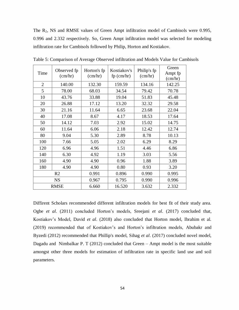
54

The R2, NS and RMSE values of Green Ampt infiltration model of Cambisols were 0.995,

0.996 and 2.332 respectively. So, Green Ampt infiltration model was selected for modeling

infiltration rate for Cambisols followed by Philip, Horton and Kostiakov.

Table 5: Comparison of Average Observed infiltration and Models Value for Cambisols

Time Observed fp

(cm/hr)

Horton's fp

(cm/hr)

Kostiakov's

fp (cm/hr)

Philip's fp

(cm/hr)

Green

Ampt fp

(cm/hr)

2 140.00 132.30 159.59 134.16 142.25

5 78.00 68.03 34.54 79.42 70.78

10 43.76 33.88 19.04 51.83 45.48

20 26.88 17.12 13.20 32.32 29.58

30 21.16 11.64 6.65 23.68 22.04

40 17.08 8.67 4.17 18.53 17.64

50 14.12 7.03 2.92 15.02 14.75

60 11.64 6.06 2.18 12.42 12.74

80 9.04 5.30 2.89 8.78 10.13

100 7.66 5.05 2.02 6.29 8.29

120 6.96 4.96 1.51 4.46 6.86

140 6.30 4.92 1.19 3.03 5.56

160 4.90 4.90 0.96 1.88 3.89

180 4.90 4.90 0.80 0.93 3.20

R2 0.991 0.896 0.990 0.995

NS 0.967 0.795 0.990 0.996

RMSE 6.660 16.520 3.632 2.332

Diffirent Scholars recommended different infiltration models for best fit of their study area.

Ogbe et al. (2011) concluded Horton‟s models, Sreejani et al. (2017) concluded that,

Kostiakov‟s Model, David et al. (2018) also concluded that Horton model, Ibrahim et al.

(2019) recommended that of Kostiakov‟s and Horton‟s infiltration models, Abubakr and

Byzedi (2012) recommended that Phillip's model, Sihag et al. (2017) concluded novel model,

Dagadu and Nimbalkar P. T (2012) concluded that Green – Ampt model is the most suitable

amongst other three models for estimation of infiltration rate in specific land use and soil

parameters.

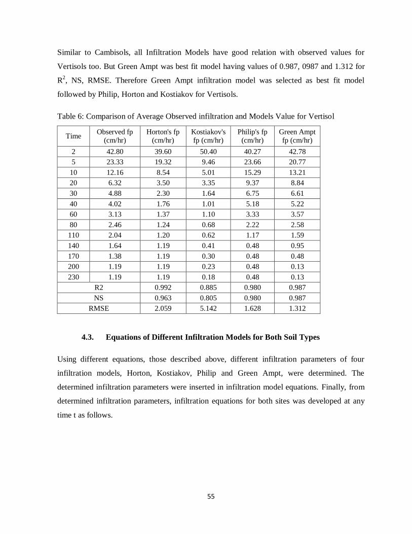
55

Similar to Cambisols, all Infiltration Models have good relation with observed values for

Vertisols too. But Green Ampt was best fit model having values of 0.987, 0987 and 1.312 for

R2, NS, RMSE. Therefore Green Ampt infiltration model was selected as best fit model

followed by Philip, Horton and Kostiakov for Vertisols.

Table 6: Comparison of Average Observed infiltration and Models Value for Vertisol

Time Observed fp

(cm/hr) Horton's fp

(cm/hr) Kostiakov's fp (cm/hr)

Philip's fp (cm/hr)


2 42.80 39.60 50.40 40.27 42.78

5 23.33 19.32 9.46 23.66 20.77

10 12.16 8.54 5.01 15.29 13.21

20 6.32 3.50 3.35 9.37 8.84

30 4.88 2.30 1.64 6.75 6.61

40 4.02 1.76 1.01 5.18 5.22

60 3.13 1.37 1.10 3.33 3.57

80 2.46 1.24 0.68 2.22 2.58

110 2.04 1.20 0.62 1.17 1.59

140 1.64 1.19 0.41 0.48 0.95

170 1.38 1.19 0.30 0.48 0.48

200 1.19 1.19 0.23 0.48 0.13

230 1.19 1.19 0.18 0.48 0.13

R2 0.992 0.885 0.980 0.987

NS 0.963 0.805 0.980 0.987

RMSE 2.059 5.142 1.628 1.312

4.3. Equations of Different Infiltration Models for Both Soil Types

Using different equations, those described above, different infiltration parameters of four

infiltration models, Horton, Kostiakov, Philip and Green Ampt, were determined. The

determined infiltration parameters were inserted in infiltration model equations. Finally, from

determined infiltration parameters, infiltration equations for both sites was developed at any

time t as follows.

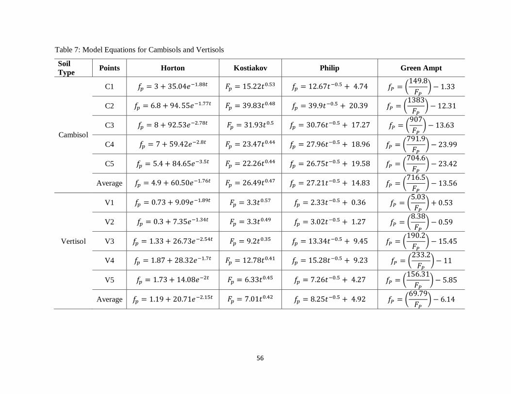
56

Table 7: Model Equations for Cambisols and Vertisols

Soil

Type Points Horton Kostiakov Philip Green Ampt

Cambisol

C1 (

)

C2 (

)

C3 (

)

C4 (

)

C5 (

)

Average (

)

Vertisol

V1 (

)

V2 (

)

V3 (

)

V4 (

)

V5 (

)

Average (

)

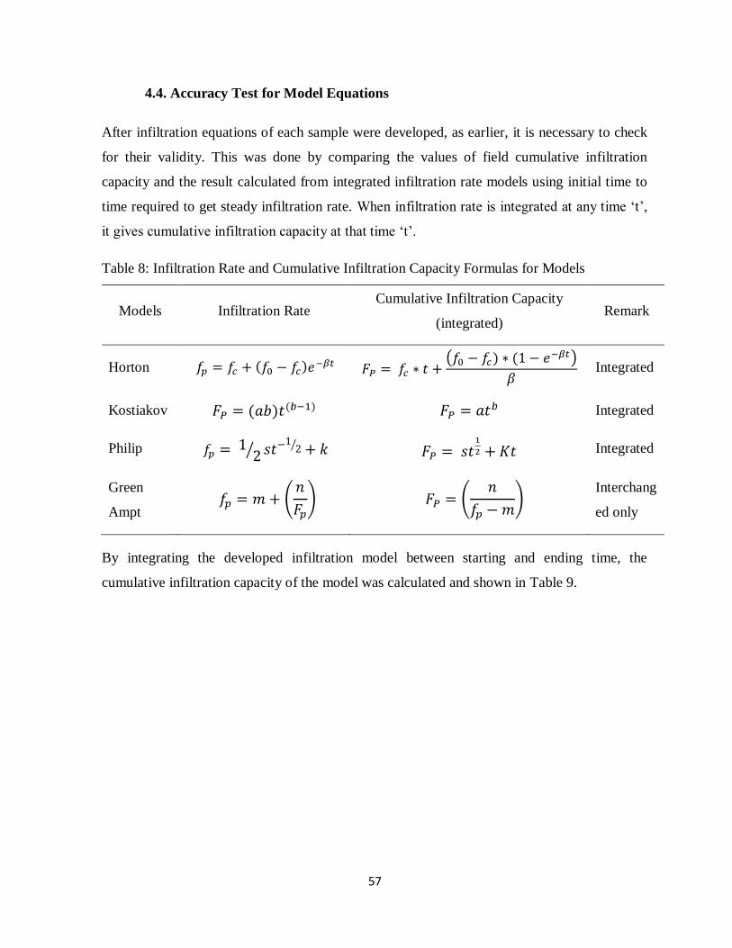
57

4.4. Accuracy Test for Model Equations

After infiltration equations of each sample were developed, as earlier, it is necessary to check

for their validity. This was done by comparing the values of field cumulative infiltration

capacity and the result calculated from integrated infiltration rate models using initial time to

time required to get steady infiltration rate. When infiltration rate is integrated at any time „t‟,

it gives cumulative infiltration capacity at that time „t‟.

Table 8: Infiltration Rate and Cumulative Infiltration Capacity Formulas for Models

Models Infiltration Rate Cumulative Infiltration Capacity

(integrated) Remark

Horton

( )

Integrated

Kostiakov Integrated

Philip ⁄

⁄

Integrated

Green

Ampt (

) (

)

Interchang

ed only

By integrating the developed infiltration model between starting and ending time, the

cumulative infiltration capacity of the model was calculated and shown in Table 9.

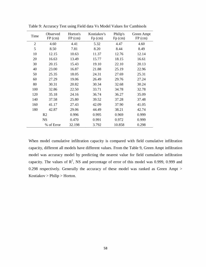
58

Table 9: Accuracy Test using Field data Vs Model Values for Cambisols

When model cumulative infiltration capacity is compared with field cumulative infiltration

capacity, different all models have different values. From the Table 9, Green Ampt infiltration

model was accuracy model by predicting the nearest value for field cumulative infiltration

capacity. The values of R2, NS and percentage of error of this model was 0.999, 0.999 and

0.298 respectively. Generally the accuracy of these model was ranked as Green Ampt >

Kostiakov > Philip > Horton.

Time Observed FP (cm)

Horton's FP (cm)

Kostiakov's Fp (cm)

Philip's Fp (cm)

Green Ampt FP (cm)

2 4.60 4.41 5.32 4.47 4.60

5 8.50 7.81 8.20 8.44 8.49

10 12.15 10.63 11.37 12.76 12.14

20 16.63 13.49 15.77 18.15 16.61

30 20.15 15.43 19.10 22.10 20.13

40 23.00 16.87 21.88 25.19 22.96

50 25.35 18.05 24.31 27.69 25.31

60 27.29 19.06 26.49 29.76 27.24

80 30.31 20.82 30.34 32.68 30.24

100 32.86 22.50 33.71 34.78 32.78

120 35.18 24.16 36.74 36.27 35.09

140 37.58 25.80 39.52 37.28 37.48

160 41.17 27.43 42.09 37.90 41.05

180 42.87 29.06 44.49 38.21 42.74

R2 0.996 0.995 0.969 0.999

NS 0.470 0.991 0.972 0.999

% of Error 32.198 3.792 10.858 0.298

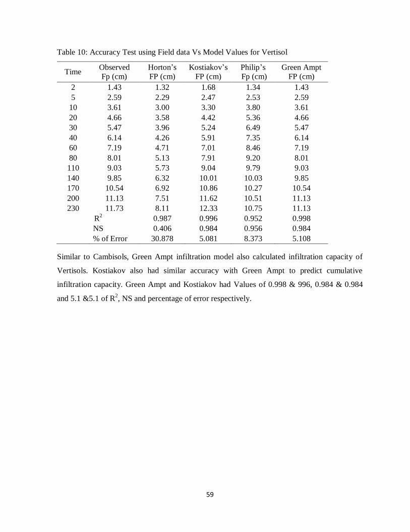
59

Table 10: Accuracy Test using Field data Vs Model Values for Vertisol

Time Observed

Fp (cm)

Horton‟s

FP (cm)

Kostiakov‟s

FP (cm)

Philip‟s

Fp (cm)

Green Ampt

FP (cm)

2 1.43 1.32 1.68 1.34 1.43

5 2.59 2.29 2.47 2.53 2.59

10 3.61 3.00 3.30 3.80 3.61

20 4.66 3.58 4.42 5.36 4.66

30 5.47 3.96 5.24 6.49 5.47

40 6.14 4.26 5.91 7.35 6.14

60 7.19 4.71 7.01 8.46 7.19

80 8.01 5.13 7.91 9.20 8.01

110 9.03 5.73 9.04 9.79 9.03

140 9.85 6.32 10.01 10.03 9.85

170 10.54 6.92 10.86 10.27 10.54

200 11.13 7.51 11.62 10.51 11.13

230 11.73 8.11 12.33 10.75 11.13

R2 0.987 0.996 0.952 0.998

NS 0.406 0.984 0.956 0.984

% of Error 30.878 5.081 8.373 5.108

Similar to Cambisols, Green Ampt infiltration model also calculated infiltration capacity of

Vertisols. Kostiakov also had similar accuracy with Green Ampt to predict cumulative

infiltration capacity. Green Ampt and Kostiakov had Values of 0.998 & 996, 0.984 & 0.984

and 5.1 &5.1 of R2, NS and percentage of error respectively.

60

5. CONCLUSION AND RECOMMENDATION

Under this section, the results of both Cambisols and Vertisol infiltration capacity, the values

of determined infiltration parameters of Horton, Kostiakov, Philip and Green Ampt infiltration

models, inter comparison of the models were concluded. The best fit infiltration, the valid

developed infiltration model and the use of this valid infiltration model for future use were

also recommended.

5.1. Conclusion

The result of the study was showed that, there is a difference in infiltration rate from one

point to another at both, Cambisols and vertisol. Constant infiltration rate of Cambisols are 3,

6.8, 8, 7, 5.4 cm/hr for sample C1, C2, C3, C4, and C5 respectively. Similarly, constant

infiltration rate for Vertisol are 0.73, 0.3, 1.33, 1.87, 1.73 cm/hr for point V1, V2, V3, V4, and

V5 respectively. This result showed that infiltration rate is higher in Cambisols than Vertisol.

Infiltration parameters of four infiltration models, Horton, Kostiakov, Philip and Green Ampt,

were determined from field infiltration rate and cumulative infiltration using graph. These

infiltration parameters were not similar for different infiltration points and soil types. This

result showed that, the highest initial infiltration rate of vertisol is near to the lowest initial

infiltration rate of Cambisols. From Kostiakov Infiltration Model, the values of local

parameter „b‟ are ranged from 0.41 to 0.57 which is above zero and below one at all points

and soil types. Similarly local parameter „a‟ are ranged from 3.3 to 39.83 which above zero for

two soil types. These two conditions satisfy infiltration rule of Kostiakov Model. The function

of soil suction potential (S) of Philip Infiltration Model is between 4.65 and 79.80 which is

greater than zero. This shows the soil at each point and soil type has potential to suck water.

And hydraulic conductivity of soil is different for all points. The lowest and highest hydraulic

conductivity is 0.36hr- and 20.39hr

-. Hydraulic conductivity of Cambisols, which is ranged

from 14.74 to 20.39 hr-, is greater than Vertisols which is ranged from 0.36 to 9.45 hr

-.

The inter comparison of, Horton, Kostiakov, Philip and Green Ampt infiltration models

related to field collected infiltration rate using both R2, NS and RMSE, showed that, Green

Ampt infiltration model is best fit models followed by Philip, Horton and Kostiakov for both

61

Cambisols and Vertisos. The Values of R2, NS and RMSE of Green Ampt were 0.995, 0.996

and 2.332 respectively for Cambisols. This finding implied that, there is strong relationship

between infiltration rate which was collected from the field and calculated values of the

models. In similar way, the values of RMSE are 2.332, 3.632, 6.660 and 16.520 for Green

Ampt, Philip, Horton and Kostiakov infiltration models respectively. And result of the R2, NS

and and RMSE values of Green Ampt infiltration model were 0.987, 0987 and 1.312 for

Vertisols, which also implied that, there is strong relationship between infiltration rate which

was collected from the field and calculated using this model.

Cumulative infiltration rate collected from field and developed models were compared for

validation of the developed infiltration model. From this, the result showed that Green Ampt

infiltration model gives the nearest value of field cumulative infiltration capacity of soil. The

values of R2, NS and percentage of error of this model was 0.999, 0.999 and 0.298

respectively. Similar to Cambisols, Green Ampt infiltration model also calculated infiltration

capacity of Vertisols. Kostiakov also had similar accuracy with Green Ampt to predict

cumulative infiltration capacity. Green Ampt and Kostiakov had Values of 0.998 & 996, 0.984

& 0.984 and 5.1 &5.1 of R2, NS and percentage of error respectively. Generally the accuracy

of these model was ranked as Green Ampt > Kostiakov > Philip > Horton. Therefore this

model can be used to calculate the infiltration capacity of both Cambisols and Vertisols, which

are the most dominant soil types of Upper Awash Basin.

5.2. Recommendation

Even though, all models have good relation with observed values, Green Ampt Model is the

best fitting model for both soils showing highest degree of R2 and NS and minimum RMSE.

Therefore, Green Ampt infiltration model is recommended that it is best model to calculate

infiltration rate of both Cambisols and Vertisols for dry season. Since infiltration behavior of

the soil directly determines the essential variables such as inflow rate, length of run,

application time, depth of percolation, and tail water run-off in irrigation systems, this model

is also useful to design, operation, management, and hydraulic evaluation of on-farm water

applications. But further study is necessary to identify other hydrologic processes by

addressing additional land use/coves, and both dry and wet season.

62

REFERENCES

Abdulkadir, M. N. Wuddivira, N. Abdu1 and O. J. Mudiare (2011). Use of Horton Infiltration

Model in Estimating Infiltration Characteristics of an Alfisol in the Northern Guinea

Savanna of Nigeria. Journal of Agricultural Science and Technology,

https://www.researchgate.net/publication/215531912. 926-931 PP.

Abubakr Rahimi and Motalleb Byzedi (2012): The Evaluation and Determining of Soil

Infiltration Models Coefficients. Australian Journal of Basic and Applied Sciences,

6(6): 94-98, 2012. ISSN 1991-8178

Adindu Ruth Uloma, Akoma Chigozie Samuel, Igbokwe Kelechi Kingsley (2014). Estimation

of Kostiakov’s Infiltration Model Parameters of Some Sandy Loam Soils of Ikwuano –

Umuahia, Nigeria. Open Transactions on Geosciences Volume 1, Number 1. Online

Publication. 34-38 PP.

Antigha, N. R. B. & Essien, I. E. (2007). The Relationship between Infiltration rate and

Hydraulic Conductivity of some soils of Akpabuyo Local Government Area of Cross

River State –Nigeria. Global Journal of Pure and Applied Science

www.ijastnet.com/journals/Vol_2.../10.pdf. Accessed 1-02-2013.

Av Sondre N. Balstad, Jardar Lohne, Tone M. Muthanna1 og Edvard Sivertsen. Seasonal

variations in infiltration in cold climate raingardens – a case study from Norway.

Department of Civil and Environmental Engineering, NTNU, 7491-Trondheim,

Norway. SINTEF Byggforsk, 7034-Trondheim, Norway. 1-13 PP.

Balraj Singh, Parveen Sihag, Diwan Singh (2014). Study of Infiltration Characteristics of

Locally Soils. Journal of Civil Engineering and Environmental Technology, Volume 1,

Number 5. Krishi Sanskriti Publications, http://www.krishisanskriti.org/jceet.html, 9 –

13 PP. Bayero University farm, Kano-Nigeria. IOP Conf. Series: Materials Science

and Engineering 527 (2019) 012013 doi:10.1088/1757-899X/527/1/012013

Dagadu, J.S. Nimbalkar P. T. (2012), Infiltration Studies Of Different Soils Under Different

Soil Conditions And Comparison Of Infiltration Models With Field Data.

https://www.researchgate.net/publication/215531912

http://www.ijastnet.com/journals/Vol_2.../10.pdf.%20Accessed%201-02-2013

http://www.krishisanskriti.org/jceet.html

63

IJAET/Vol.III/ Issue II/ EISSN 0976-3945, www.technicaljournalsonline.com/. 154-

157 PP.

Eze Bassey Eze, Devalsam Imoke Eni & Oko (2011). Evaluation of the Infiltration Capacity

of Soils in Akpabuyo Local Government Area of Cross River, Nigeria. Journal of

Geography and Geology Vol. 3, No. 1. Canadian Center of Science and Education, 1-

11 PP.

Freund and Rahardjo (1993). Soil mechanics for unsaturated soils. D. G. Fredlund and H.

Rahardjo. Librury of Congress Cataloging in Publication Data: Fredlund, D. G.

(Delwyn G.), 1940- 1993. New York.

Ghanshyam Tikaram Patle, Tatung Taka Sikar, Kishan Singh Rawat & Sudhir Kumar Singh

(2018). Estimation of infiltration rate from soil properties using regression model for

cultivated land. Geology, Ecology, and Landscapes, ISSN:

http://www.tandfonline.com/loi/tgel20, Informa UK Limited, trading as Taylor &

Francis Group on behalf of the International Water, Air & Soil Conservation Society

(INWASCON). 15 PP.

Haghiabi, A. H., A bedi-Koupai, J.,Heidarpour, M. and Mohammadzadeh-Habili, J. (2011). A

new method for estimating the parameters of Kostiakov and modified Kostiakov

infiltration equations. World Applied Sciences Journal. 15(1): 129 –135

Hsu, S. M., Ni, C. F. and Hung, P. F. (2002). Assessment of three infiltration formulas based

on model fitting on Richards equation. Journal of hydrologic Engineering. 7(5): 373 –

379

Ibrahim, S K Lary, M D Zakari, N M Nasidi and M N Yahya (2013): Performance evaluation

of some selected infiltration models at

Ieke Wulan Ayu, Sugeng Prijono, and Soemarno (2013). Assessment of Infiltration Rate under

Different Drylands Types in Unter-Iwes Subdistrict Sumbawa Besar, Indonesia.

Journal of Natural Sciences Research, www.iiste.org ISSN 2224-3186 (Paper) ISSN

2225-0921 (Online) Vol.3, No.10. 71-76 PP.

http://www.technicaljournalsonline.com/

http://www.tandfonline.com/loi/tgel20

http://www.iiste.org/

64

Imran Arshad, Asadullah Sarki, Zaheer Ahmed Khan (2015): Analysis of Water Transmission

Behaviour in Sandy Loam Soil under Different Tillage Operations of Mould Board

Plough applying /Using Different Infiltration Models.

https://www.researchgate.net/publication/304347155. Volume 3 Issue VII, July 2015:

13.98 ISSN: 2321-9653

Jagdale Satyawan Dagadu, Nimbalkar P. T., (2012). Infiltration Studies of Different Soils

under Different Soil Conditions and Comparison of Infiltration.

K Subramanya. Engineering Hydrology. Third reprint (2009). Tata McGraw-Hill, third

edition. pp: 80-91

Lal and Shukla (2005). Principle of Soil Physics. Published in the Taylor & Francis e-Library,

2005. ISBN: 0-8247-5324-0. New York

Mahbub Hasan, Tamara Chowdhury, Mebougna Drabo, Aschalew Kassu, Chance Glenn

(2015). Modeling of Infiltration Characteristics by Modified Kostiakov Method.

Journal of Water Resource and Protection, 7, 1309-1317.

http://dx.doi.org/10.4236/jwarp.2015.716106. 1310-1317 PP.

Martina Vicanová, František Toman, Tomáš Mašícek, Petra Oppeltová (2011). Comparative

study of soil infiltration capacity at selected sites. Commission of Technical Rural

Infrastructure, Polish Academy of Sciences, Cracow Branch, [online]

http://www.mapy.cz. 17-30 PP.

Mishra, S. K., Tyagi, J. V. and Singh, V. P. (2013). Comparison of infiltration models.

Journal of Hydrological Processes. 17: 2629 – 2652. International Journal of

Advanced Engineering Technology E-ISSN 0976-3945 IJAET/Vol.III/ Issue II/April-

June, 2012/154-157.

Musa, J. J. and Adeoye, P. A. (2010). Adaptability of infiltration equations to the soils of the

Permanent Site Farm of the Federal University of Technology, Minna, in the Guinea

Savannah Zone of Nigeria. Journal of Technology. 14(2): 147 – 155

https://www.researchgate.net/publication/304347155

http://dx.doi.org/10.4236/jwarp.2015.716106.%201310-1317

http://www.mapy.cz/

65

Nitin P Sonaje (2013): Modeling of Infiltration Process – A Review. Indian Journal of Applied

Research · October 2013 DOI: 10.15373/2249555X/SEPT2013/69

Ogbe, V. B., Jayeoba, O.J. and Ode, S. O (2011). Comparison of Four Soil Infiltration Models

on A Sandy Soil In Lafia, Southern Guinea Savanna Zone of Nigeria. ISSN: 0794-

5213. Online copy available at www.patnsukjournal.net/currentissue. 116-126 PP.

Oku, E. and Aiyelari, A. (2011). Predictability of Philip and Kostiakov infiltration model

under inceptisols in the Humid Forest Zone, Nigeria. Kasetsart Journal (Natural

Science), 45: 594 -602

ParveenSihag, N.K. Tiwari, SubodhRanjan(2017): Estimation and inter-comparison of

infiltration models. Journal of the International Water Association, Vol. 31, pp:34–43,

April 2017

Rashidi, M., Ahmadbeyki, A., & Hajiaghaei, A. (2014). Prediction of soil infiltration rate

based on some physical properties of soil. American-Eurasian Journal of Agricultural

and Environmental Science, 14(12), 1359–1367 PP.

Sarmadian, F., & Taaghizadeh-Mehrjardi, R. (2014). Estimation of infiltration rate and deep

percolation water using feed-forward neural networks in Gorgan province. Eurasian

Journal of Soil Science, 3(1), 1–6 PP.

Sreejani TP, Abhishek D, Srinivasa Rao GVR, Abbulu Y (2017). A Study on Infiltration

Characteristics of Soils at Andhra University Campus Visakhapatnam. International

Journal of Environmental Research and Development. ISSN 2249-3131 Volume 7.

Research India Publications http://www.ripublication.com. 29-44 PP.

Sunith John David, Akash Shaji, Ashmy M S, Neenu Raju, and Nimisha Sebastian. (2018). A

Novel Methodology for Infiltration Model Studies. International Journal of Engineering

Technologies and Management Research, 5(3), 190-199. DOI:

10.5281/zenodo.1218178.

Tsuyoshi Miyazaki (2006). Water flow in soils. 2nd

edition. Published in 2006 by CRC Press.

New York 2006

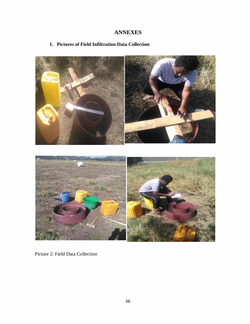
http://www.patnsukjournal.net/currentissue

http://www.ripublication.com/

66

ANNEXES

1. Pictures of Field Infiltration Data Collection

Picture 2: Field Data Collection

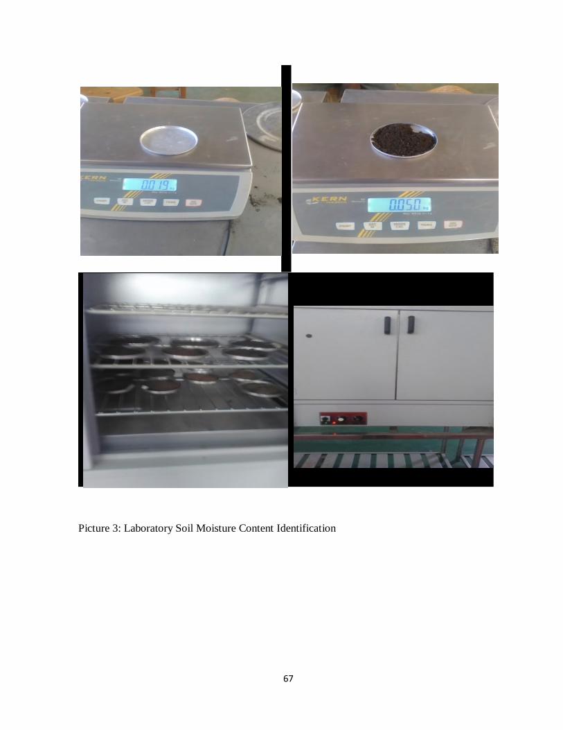
67

Picture 3: Laboratory Soil Moisture Content Identification

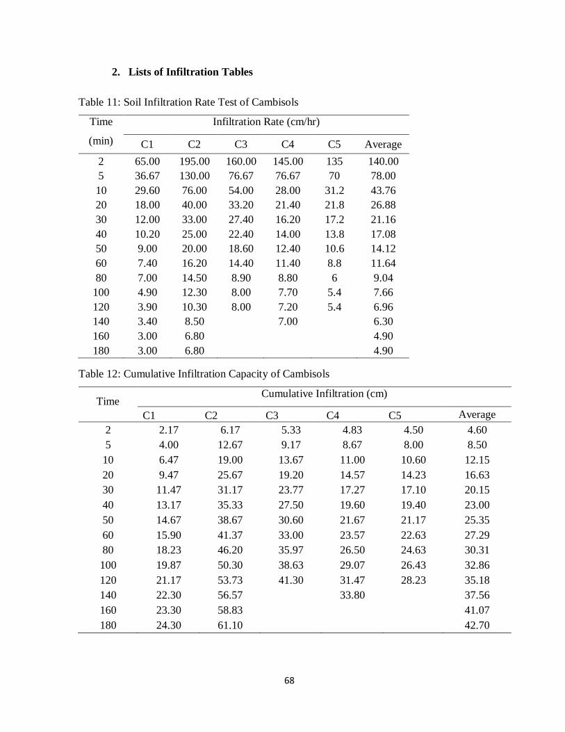
68

2. Lists of Infiltration Tables

Table 11: Soil Infiltration Rate Test of Cambisols

Time

(min)


C1 C2 C3 C4 C5 Average

2 65.00 195.00 160.00 145.00 135 140.00

5 36.67 130.00 76.67 76.67 70 78.00

10 29.60 76.00 54.00 28.00 31.2 43.76

20 18.00 40.00 33.20 21.40 21.8 26.88

30 12.00 33.00 27.40 16.20 17.2 21.16

40 10.20 25.00 22.40 14.00 13.8 17.08

50 9.00 20.00 18.60 12.40 10.6 14.12

60 7.40 16.20 14.40 11.40 8.8 11.64

80 7.00 14.50 8.90 8.80 6 9.04

100 4.90 12.30 8.00 7.70 5.4 7.66

120 3.90 10.30 8.00 7.20 5.4 6.96

140 3.40 8.50 7.00 6.30

160 3.00 6.80 4.90

180 3.00 6.80 4.90

Table 12: Cumulative Infiltration Capacity of Cambisols

Time Cumulative Infiltration (cm)

C1 C2 C3 C4 C5 Average

2 2.17 6.17 5.33 4.83 4.50 4.60

5 4.00 12.67 9.17 8.67 8.00 8.50

10 6.47 19.00 13.67 11.00 10.60 12.15

20 9.47 25.67 19.20 14.57 14.23 16.63

30 11.47 31.17 23.77 17.27 17.10 20.15

40 13.17 35.33 27.50 19.60 19.40 23.00

50 14.67 38.67 30.60 21.67 21.17 25.35

60 15.90 41.37 33.00 23.57 22.63 27.29

80 18.23 46.20 35.97 26.50 24.63 30.31

100 19.87 50.30 38.63 29.07 26.43 32.86

120 21.17 53.73 41.30 31.47 28.23 35.18

140 22.30 56.57 33.80 37.56

160 23.30 58.83 41.07

180 24.30 61.10 42.70

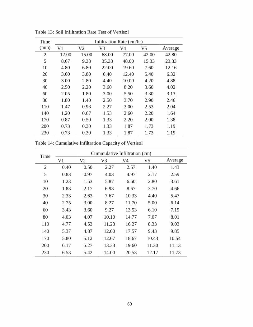
69

Table 13: Soil Infiltration Rate Test of Vertisol

Time

(min)


V1 V2 V3 V4 V5 Average

2 12.00 15.00 68.00 77.00 42.00 42.80

5 8.67 9.33 35.33 48.00 15.33 23.33

10 4.80 6.80 22.00 19.60 7.60 12.16

20 3.60 3.80 6.40 12.40 5.40 6.32

30 3.00 2.80 4.40 10.00 4.20 4.88

40 2.50 2.20 3.60 8.20 3.60 4.02

60 2.05 1.80 3.00 5.50 3.30 3.13

80 1.80 1.40 2.50 3.70 2.90 2.46

110 1.47 0.93 2.27 3.00 2.53 2.04

140 1.20 0.67 1.53 2.60 2.20 1.64

170 0.87 0.50 1.33 2.20 2.00 1.38

200 0.73 0.30 1.33 1.87 1.73 1.19

230 0.73 0.30 1.33 1.87 1.73 1.19

Table 14: Cumulative Infiltration Capacity of Vertisol

Time Cummulative Infiltration (cm)

V1 V2 V3 V4 V5 Average

2 0.40 0.50 2.27 2.57 1.40 1.43

5 0.83 0.97 4.03 4.97 2.17 2.59

10 1.23 1.53 5.87 6.60 2.80 3.61

20 1.83 2.17 6.93 8.67 3.70 4.66

30 2.33 2.63 7.67 10.33 4.40 5.47

40 2.75 3.00 8.27 11.70 5.00 6.14

60 3.43 3.60 9.27 13.53 6.10 7.19

80 4.03 4.07 10.10 14.77 7.07 8.01

110 4.77 4.53 11.23 16.27 8.33 9.03

140 5.37 4.87 12.00 17.57 9.43 9.85

170 5.80 5.12 12.67 18.67 10.43 10.54

200 6.17 5.27 13.33 19.60 11.30 11.13

230 6.53 5.42 14.00 20.53 12.17 11.73

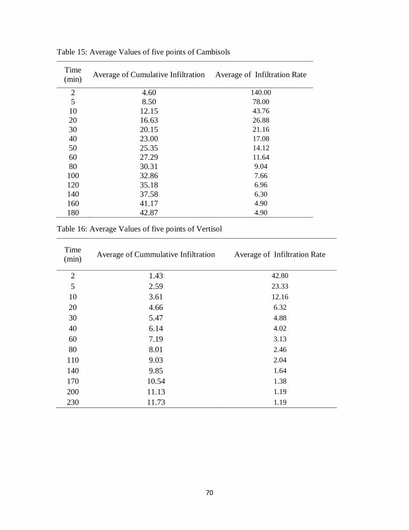
70

Table 15: Average Values of five points of Cambisols

Time

(min) Average of Cumulative Infiltration Average of Infiltration Rate

2 4.60 140.00

5 8.50 78.00

10 12.15 43.76

20 16.63 26.88

30 20.15 21.16

40 23.00 17.08

50 25.35 14.12

60 27.29 11.64

80 30.31 9.04

100 32.86 7.66

120 35.18 6.96

140 37.58 6.30

160 41.17 4.90

180 42.87 4.90

Table 16: Average Values of five points of Vertisol

Time

(min) Average of Cummulative Infiltration Average of Infiltration Rate

2 1.43 42.80

5 2.59 23.33

10 3.61 12.16

20 4.66 6.32

30 5.47 4.88

40 6.14 4.02

60 7.19 3.13

80 8.01 2.46

110 9.03 2.04

140 9.85 1.64

170 10.54 1.38

200 11.13 1.19

230 11.73 1.19

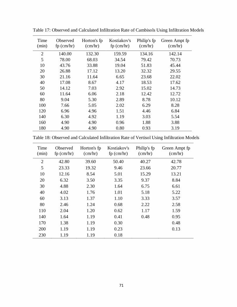
71

Table 17: Observed and Calculated Infiltration Rate of Cambisols Using Infiltration Models

Time

(min)

Observed

fp (cm/hr)

Horton's fp

(cm/hr)

Kostiakov's

fp (cm/hr)

Philip's fp

(cm/hr)

Green Ampt fp

(cm/hr)

2 140.00 132.30 159.59 134.16 142.14

5 78.00 68.03 34.54 79.42 70.73

10 43.76 33.88 19.04 51.83 45.44

20 26.88 17.12 13.20 32.32 29.55

30 21.16 11.64 6.65 23.68 22.02

40 17.08 8.67 4.17 18.53 17.62

50 14.12 7.03 2.92 15.02 14.73

60 11.64 6.06 2.18 12.42 12.72

80 9.04 5.30 2.89 8.78 10.12

100 7.66 5.05 2.02 6.29 8.28

120 6.96 4.96 1.51 4.46 6.84

140 6.30 4.92 1.19 3.03 5.54

160 4.90 4.90 0.96 1.88 3.88

180 4.90 4.90 0.80 0.93 3.19

Table 18: Observed and Calculated Infiltration Rate of Vertisol Using Infiltration Models

Time

(min)

Observed

fp (cm/hr)

Horton's fp

(cm/hr)

Kostiakov's

fp (cm/hr)

Philip's fp

(cm/hr)

Green Ampt fp

(cm/hr)

2 42.80 39.60 50.40 40.27 42.78

5 23.33 19.32 9.46 23.66 20.77

10 12.16 8.54 5.01 15.29 13.21

20 6.32 3.50 3.35 9.37 8.84

30 4.88 2.30 1.64 6.75 6.61

40 4.02 1.76 1.01 5.18 5.22

60 3.13 1.37 1.10 3.33 3.57

80 2.46 1.24 0.68 2.22 2.58

110 2.04 1.20 0.62 1.17 1.59

140 1.64 1.19 0.41 0.48 0.95

170 1.38 1.19 0.30 0.48

200 1.19 1.19 0.23 0.13

230 1.19 1.19 0.18

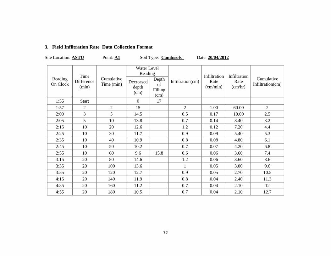
72

3. Field Infiltration Rate Data Collection Format

Site Location: ASTU Point: A1 Soil Type: Cambisols Date: 20/04/2012

Reading

On Clock

Time Difference

(min)

Cumulative

Time (min)

Water Level Reading

Infiltration(cm) Infiltration

Rate

(cm/min)

Infiltration Rate

(cm/hr)

Cumulative

Infiltration(cm) Decreased

depth

(cm)

Depth

of

Filling (cm)

1:55 Start 0 17

1:57 2 2 15 2 1.00 60.00 2

2:00 3 5 14.5 0.5 0.17 10.00 2.5

2:05 5 10 13.8 0.7 0.14 8.40 3.2

2:15 10 20 12.6 1.2 0.12 7.20 4.4

2:25 10 30 11.7 0.9 0.09 5.40 5.3

2:35 10 40 10.9 0.8 0.08 4.80 6.1

2:45 10 50 10.2 0.7 0.07 4.20 6.8

2:55 10 60 9.6 15.8 0.6 0.06 3.60 7.4

3:15 20 80 14.6 1.2 0.06 3.60 8.6

3:35 20 100 13.6 1 0.05 3.00 9.6

3:55 20 120 12.7 0.9 0.05 2.70 10.5

4:15 20 140 11.9 0.8 0.04 2.40 11.3

4:35 20 160 11.2 0.7 0.04 2.10 12

4:55 20 180 10.5 0.7 0.04 2.10 12.7

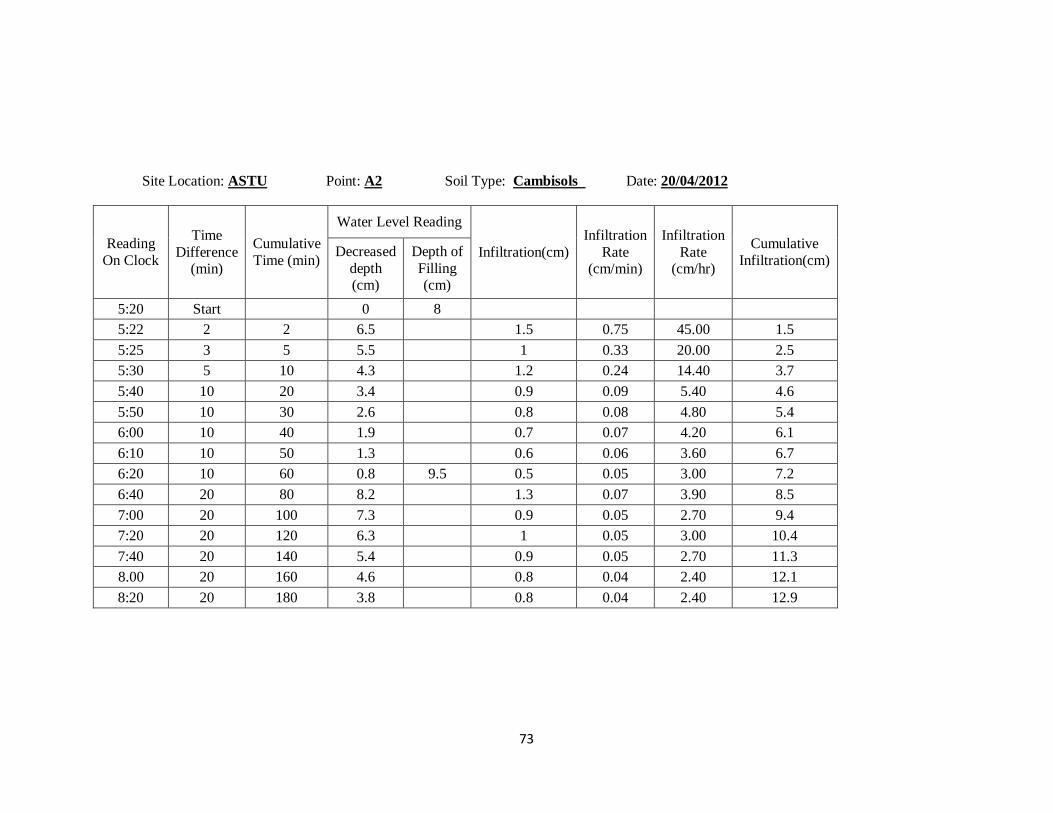
73


Reading

On Clock

Time

Difference (min)

Cumulative

Time (min)

Water Level Reading

Infiltration(cm)

Infiltration

Rate (cm/min)

Infiltration

Rate (cm/hr)

Cumulative


depth (cm)

Depth of

Filling (cm)

5:20 Start 0 8

5:22 2 2 6.5 1.5 0.75 45.00 1.5

5:25 3 5 5.5 1 0.33 20.00 2.5

5:30 5 10 4.3 1.2 0.24 14.40 3.7

5:40 10 20 3.4 0.9 0.09 5.40 4.6

5:50 10 30 2.6 0.8 0.08 4.80 5.4

6:00 10 40 1.9 0.7 0.07 4.20 6.1

6:10 10 50 1.3 0.6 0.06 3.60 6.7

6:20 10 60 0.8 9.5 0.5 0.05 3.00 7.2

6:40 20 80 8.2 1.3 0.07 3.90 8.5

7:00 20 100 7.3 0.9 0.05 2.70 9.4

7:20 20 120 6.3 1 0.05 3.00 10.4

7:40 20 140 5.4 0.9 0.05 2.70 11.3

8.00 20 160 4.6 0.8 0.04 2.40 12.1

8:20 20 180 3.8 0.8 0.04 2.40 12.9

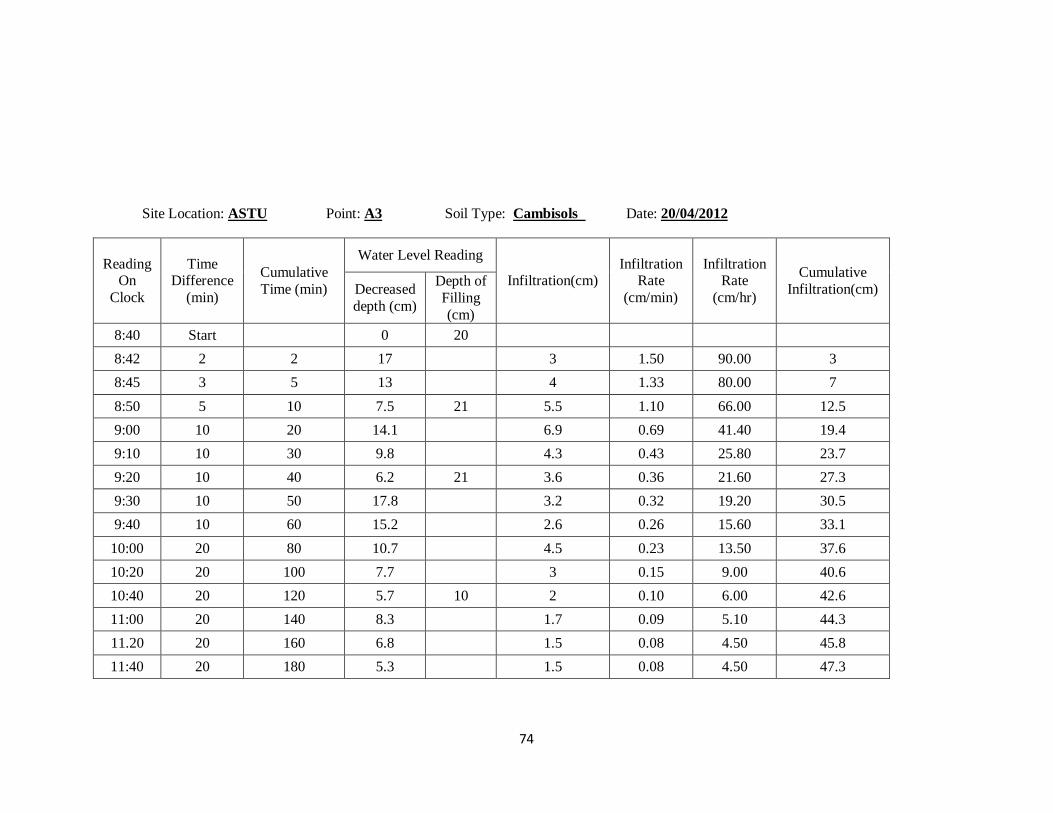
74


Reading On

Clock

Time Difference

(min)

Cumulative

Time (min)

Water Level Reading


Rate

(cm/min)

Infiltration Rate

(cm/hr)

Cumulative


depth (cm)

Depth of

Filling

(cm)

8:40 Start 0 20

8:42 2 2 17 3 1.50 90.00 3

8:45 3 5 13 4 1.33 80.00 7

8:50 5 10 7.5 21 5.5 1.10 66.00 12.5

9:00 10 20 14.1 6.9 0.69 41.40 19.4

9:10 10 30 9.8 4.3 0.43 25.80 23.7

9:20 10 40 6.2 21 3.6 0.36 21.60 27.3

9:30 10 50 17.8 3.2 0.32 19.20 30.5

9:40 10 60 15.2 2.6 0.26 15.60 33.1

10:00 20 80 10.7 4.5 0.23 13.50 37.6

10:20 20 100 7.7 3 0.15 9.00 40.6

10:40 20 120 5.7 10 2 0.10 6.00 42.6

11:00 20 140 8.3 1.7 0.09 5.10 44.3

11.20 20 160 6.8 1.5 0.08 4.50 45.8

11:40 20 180 5.3 1.5 0.08 4.50 47.3

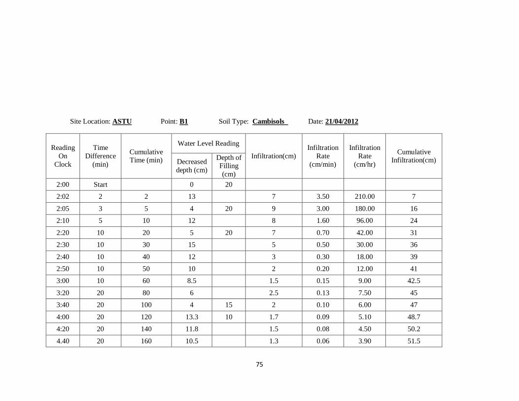
75

Site Location: ASTU Point: B1 Soil Type: Cambisols Date: 21/04/2012

Reading

On

Clock

Time

Difference

(min)

Cumulative Time (min)

Water Level Reading

Infiltration(cm)

Infiltration

Rate

(cm/min)

Infiltration

Rate

(cm/hr)

Cumulative Infiltration(cm) Decreased

depth (cm)

Depth of Filling

(cm)

2:00 Start 0 20

2:02 2 2 13 7 3.50 210.00 7

2:05 3 5 4 20 9 3.00 180.00 16

2:10 5 10 12 8 1.60 96.00 24

2:20 10 20 5 20 7 0.70 42.00 31

2:30 10 30 15 5 0.50 30.00 36

2:40 10 40 12 3 0.30 18.00 39

2:50 10 50 10 2 0.20 12.00 41

3:00 10 60 8.5 1.5 0.15 9.00 42.5

3:20 20 80 6 2.5 0.13 7.50 45

3:40 20 100 4 15 2 0.10 6.00 47

4:00 20 120 13.3 10 1.7 0.09 5.10 48.7

4:20 20 140 11.8 1.5 0.08 4.50 50.2

4.40 20 160 10.5 1.3 0.06 3.90 51.5

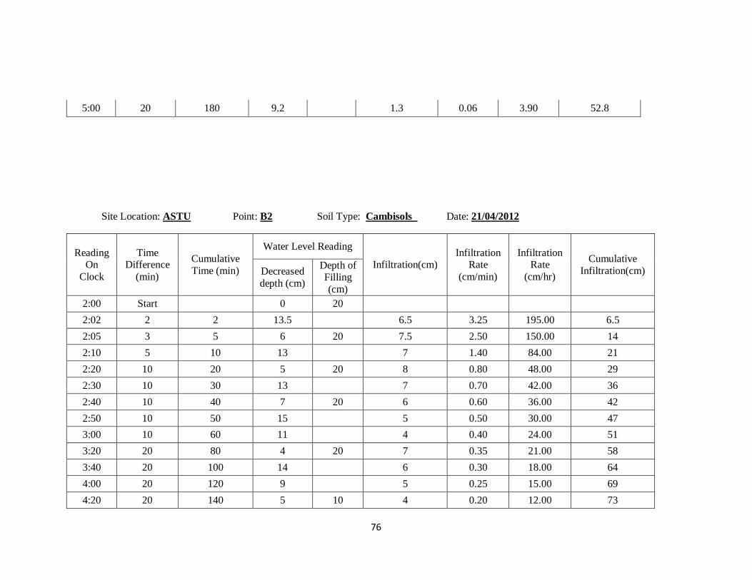
76

5:00 20 180 9.2 1.3 0.06 3.90 52.8


Reading On

Clock

Time Difference

(min)

Cumulative

Time (min)

Water Level Reading


Rate

(cm/min)

Infiltration Rate

(cm/hr)

Cumulative


depth (cm)

Depth of Filling

(cm)

2:00 Start 0 20

2:02 2 2 13.5 6.5 3.25 195.00 6.5

2:05 3 5 6 20 7.5 2.50 150.00 14

2:10 5 10 13 7 1.40 84.00 21

2:20 10 20 5 20 8 0.80 48.00 29

2:30 10 30 13 7 0.70 42.00 36

2:40 10 40 7 20 6 0.60 36.00 42

2:50 10 50 15 5 0.50 30.00 47

3:00 10 60 11 4 0.40 24.00 51

3:20 20 80 4 20 7 0.35 21.00 58

3:40 20 100 14 6 0.30 18.00 64

4:00 20 120 9 5 0.25 15.00 69

4:20 20 140 5 10 4 0.20 12.00 73

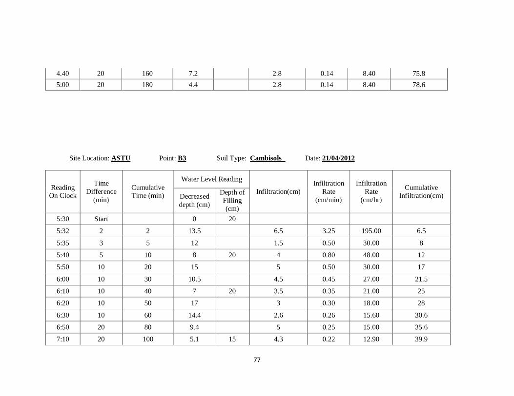
77

4.40 20 160 7.2 2.8 0.14 8.40 75.8

5:00 20 180 4.4 2.8 0.14 8.40 78.6


Reading On Clock

Time

Difference

(min)


Water Level Reading

Infiltration(cm)

Infiltration

Rate

(cm/min)

Infiltration

Rate

(cm/hr)


depth (cm)

Depth of Filling

(cm)

5:30 Start 0 20

5:32 2 2 13.5 6.5 3.25 195.00 6.5

5:35 3 5 12 1.5 0.50 30.00 8

5:40 5 10 8 20 4 0.80 48.00 12

5:50 10 20 15 5 0.50 30.00 17

6:00 10 30 10.5 4.5 0.45 27.00 21.5

6:10 10 40 7 20 3.5 0.35 21.00 25

6:20 10 50 17 3 0.30 18.00 28

6:30 10 60 14.4 2.6 0.26 15.60 30.6

6:50 20 80 9.4 5 0.25 15.00 35.6

7:10 20 100 5.1 15 4.3 0.22 12.90 39.9

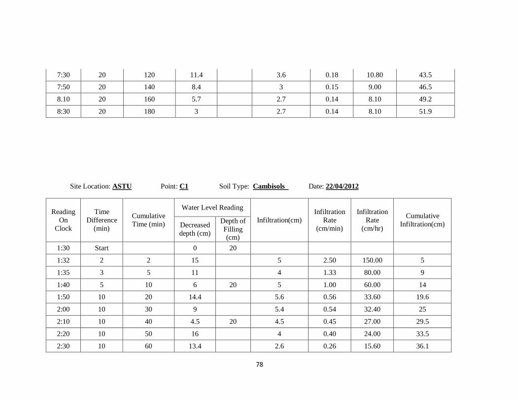
78

7:30 20 120 11.4 3.6 0.18 10.80 43.5

7:50 20 140 8.4 3 0.15 9.00 46.5

8.10 20 160 5.7 2.7 0.14 8.10 49.2

8:30 20 180 3 2.7 0.14 8.10 51.9

Site Location: ASTU Point: C1 Soil Type: Cambisols Date: 22/04/2012

Reading

On

Clock

Time

Difference

(min)

Cumulative

Time (min)

Water Level Reading

Infiltration(cm)

Infiltration

Rate

(cm/min)

Infiltration

Rate

(cm/hr)

Cumulative


depth (cm)

Depth of

Filling (cm)

1:30 Start 0 20

1:32 2 2 15 5 2.50 150.00 5

1:35 3 5 11 4 1.33 80.00 9

1:40 5 10 6 20 5 1.00 60.00 14

1:50 10 20 14.4 5.6 0.56 33.60 19.6

2:00 10 30 9 5.4 0.54 32.40 25

2:10 10 40 4.5 20 4.5 0.45 27.00 29.5

2:20 10 50 16 4 0.40 24.00 33.5

2:30 10 60 13.4 2.6 0.26 15.60 36.1

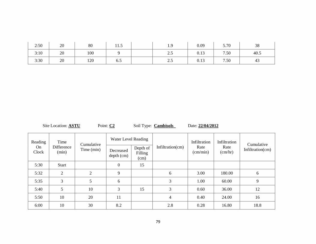
79

2:50 20 80 11.5 1.9 0.09 5.70 38

3:10 20 100 9 2.5 0.13 7.50 40.5

3:30 20 120 6.5 2.5 0.13 7.50 43


Reading

On Clock

Time

Difference (min)

Cumulative

Time (min)

Water Level Reading

Infiltration(cm)

Infiltration

Rate (cm/min)

Infiltration

Rate (cm/hr)

Cumulative


depth (cm)

Depth of Filling

(cm)

5:30 Start 0 15

5:32 2 2 9 6 3.00 180.00 6

5:35 3 5 6 3 1.00 60.00 9

5:40 5 10 3 15 3 0.60 36.00 12

5:50 10 20 11 4 0.40 24.00 16

6:00 10 30 8.2 2.8 0.28 16.80 18.8

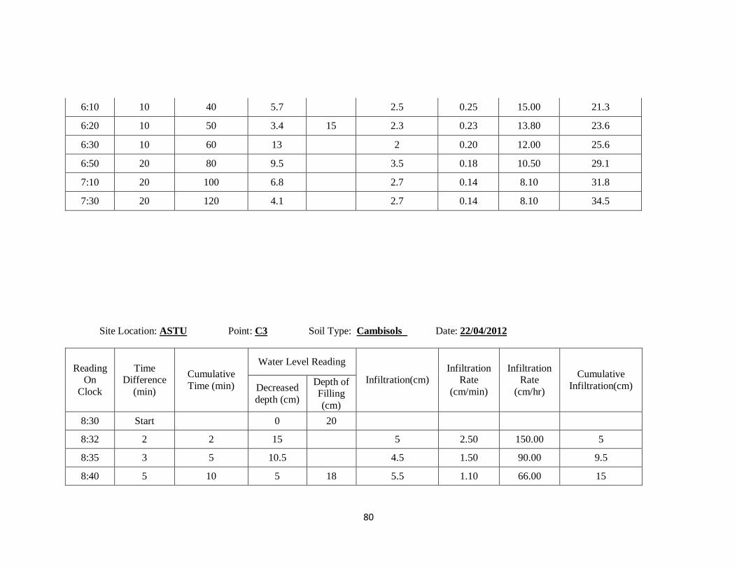
80

6:10 10 40 5.7 2.5 0.25 15.00 21.3

6:20 10 50 3.4 15 2.3 0.23 13.80 23.6

6:30 10 60 13 2 0.20 12.00 25.6

6:50 20 80 9.5 3.5 0.18 10.50 29.1

7:10 20 100 6.8 2.7 0.14 8.10 31.8

7:30 20 120 4.1 2.7 0.14 8.10 34.5


Reading On

Clock

Time Difference

(min)

Cumulative

Time (min)

Water Level Reading


Rate

(cm/min)

Infiltration Rate

(cm/hr)

Cumulative


depth (cm)

Depth of Filling

(cm)

8:30 Start 0 20

8:32 2 2 15 5 2.50 150.00 5

8:35 3 5 10.5 4.5 1.50 90.00 9.5

8:40 5 10 5 18 5.5 1.10 66.00 15

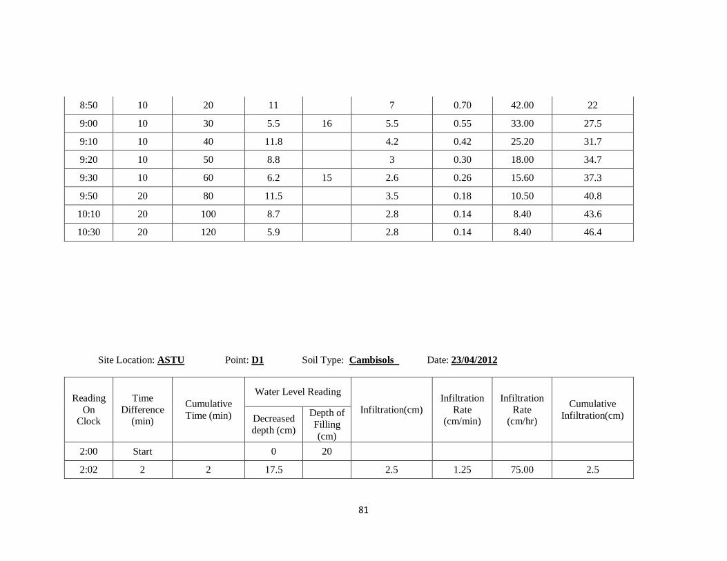
81

8:50 10 20 11 7 0.70 42.00 22

9:00 10 30 5.5 16 5.5 0.55 33.00 27.5

9:10 10 40 11.8 4.2 0.42 25.20 31.7

9:20 10 50 8.8 3 0.30 18.00 34.7

9:30 10 60 6.2 15 2.6 0.26 15.60 37.3

9:50 20 80 11.5 3.5 0.18 10.50 40.8

10:10 20 100 8.7 2.8 0.14 8.40 43.6

10:30 20 120 5.9 2.8 0.14 8.40 46.4

Site Location: ASTU Point: D1 Soil Type: Cambisols Date: 23/04/2012

Reading

On Clock

Time

Difference (min)

Cumulative

Time (min)

Water Level Reading

Infiltration(cm)

Infiltration

Rate (cm/min)

Infiltration

Rate (cm/hr)

Cumulative


depth (cm)

Depth of

Filling

(cm)

2:00 Start 0 20

2:02 2 2 17.5 2.5 1.25 75.00 2.5

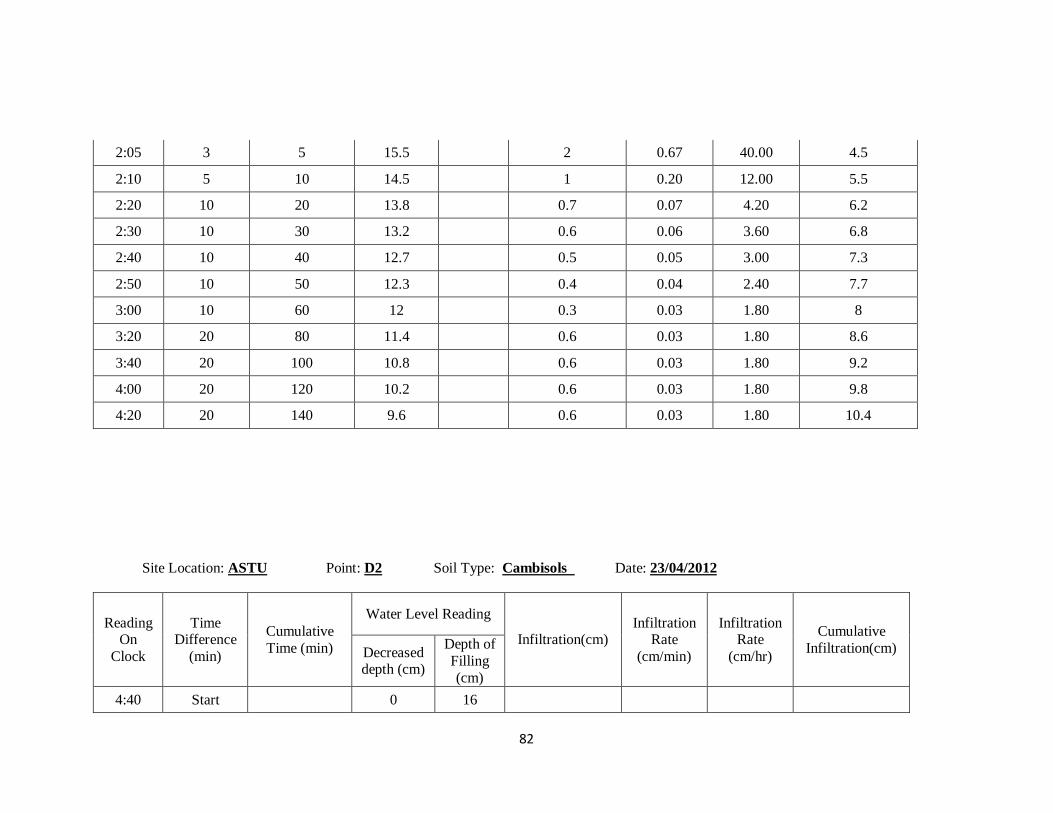
82

2:05 3 5 15.5 2 0.67 40.00 4.5

2:10 5 10 14.5 1 0.20 12.00 5.5

2:20 10 20 13.8 0.7 0.07 4.20 6.2

2:30 10 30 13.2 0.6 0.06 3.60 6.8

2:40 10 40 12.7 0.5 0.05 3.00 7.3

2:50 10 50 12.3 0.4 0.04 2.40 7.7

3:00 10 60 12 0.3 0.03 1.80 8

3:20 20 80 11.4 0.6 0.03 1.80 8.6

3:40 20 100 10.8 0.6 0.03 1.80 9.2

4:00 20 120 10.2 0.6 0.03 1.80 9.8

4:20 20 140 9.6 0.6 0.03 1.80 10.4


Reading On

Clock

Time Difference

(min)

Cumulative

Time (min)

Water Level Reading


Rate

(cm/min)

Infiltration Rate

(cm/hr)

Cumulative

Infiltration(cm) Decreased depth (cm)

Depth of

Filling

(cm)

4:40 Start 0 16

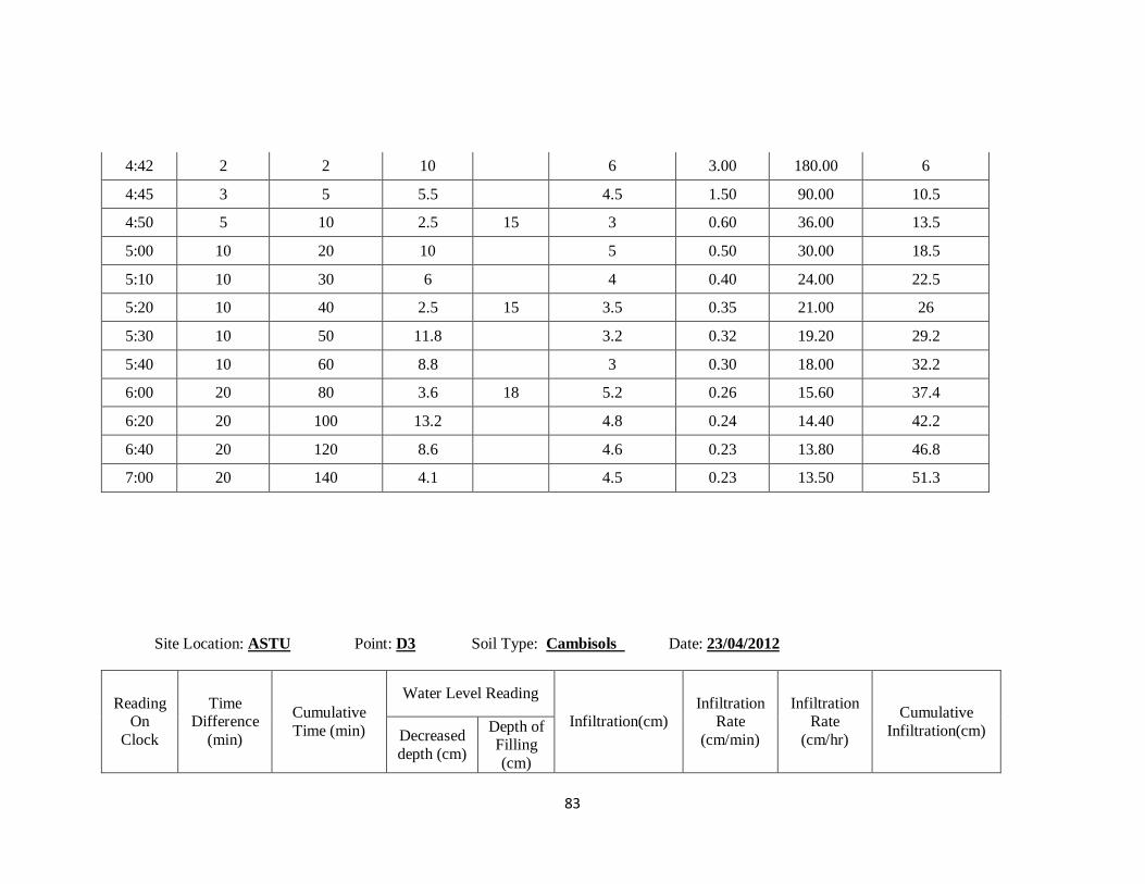
83

4:42 2 2 10 6 3.00 180.00 6

4:45 3 5 5.5 4.5 1.50 90.00 10.5

4:50 5 10 2.5 15 3 0.60 36.00 13.5

5:00 10 20 10 5 0.50 30.00 18.5

5:10 10 30 6 4 0.40 24.00 22.5

5:20 10 40 2.5 15 3.5 0.35 21.00 26

5:30 10 50 11.8 3.2 0.32 19.20 29.2

5:40 10 60 8.8 3 0.30 18.00 32.2

6:00 20 80 3.6 18 5.2 0.26 15.60 37.4

6:20 20 100 13.2 4.8 0.24 14.40 42.2

6:40 20 120 8.6 4.6 0.23 13.80 46.8

7:00 20 140 4.1 4.5 0.23 13.50 51.3


Reading On

Clock

Time Difference

(min)

Cumulative

Time (min)

Water Level Reading


Rate

(cm/min)

Infiltration Rate

(cm/hr)

Cumulative


depth (cm)

Depth of Filling

(cm)

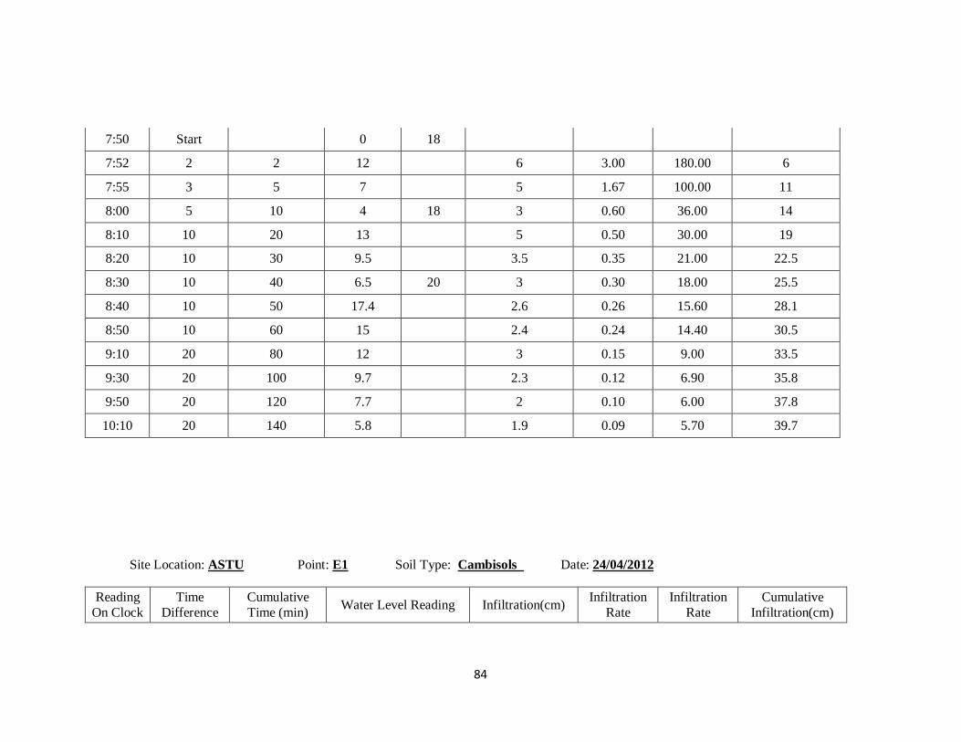
84

7:50 Start 0 18

7:52 2 2 12 6 3.00 180.00 6

7:55 3 5 7 5 1.67 100.00 11

8:00 5 10 4 18 3 0.60 36.00 14

8:10 10 20 13 5 0.50 30.00 19

8:20 10 30 9.5 3.5 0.35 21.00 22.5

8:30 10 40 6.5 20 3 0.30 18.00 25.5

8:40 10 50 17.4 2.6 0.26 15.60 28.1

8:50 10 60 15 2.4 0.24 14.40 30.5

9:10 20 80 12 3 0.15 9.00 33.5

9:30 20 100 9.7 2.3 0.12 6.90 35.8

9:50 20 120 7.7 2 0.10 6.00 37.8

10:10 20 140 5.8 1.9 0.09 5.70 39.7

Site Location: ASTU Point: E1 Soil Type: Cambisols Date: 24/04/2012

Reading

On Clock

Time

Difference

Cumulative

Time (min) Water Level Reading Infiltration(cm)

Infiltration

Rate

Infiltration

Rate

Cumulative

Infiltration(cm)

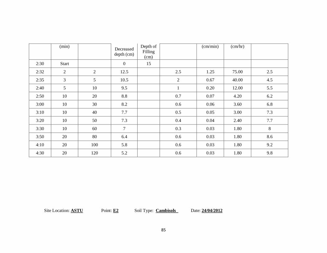
85

(min) Decreased depth (cm)

Depth of

Filling

(cm)

(cm/min) (cm/hr)

2:30 Start 0 15

2:32 2 2 12.5 2.5 1.25 75.00 2.5

2:35 3 5 10.5 2 0.67 40.00 4.5

2:40 5 10 9.5 1 0.20 12.00 5.5

2:50 10 20 8.8 0.7 0.07 4.20 6.2

3:00 10 30 8.2 0.6 0.06 3.60 6.8

3:10 10 40 7.7 0.5 0.05 3.00 7.3

3:20 10 50 7.3 0.4 0.04 2.40 7.7

3:30 10 60 7 0.3 0.03 1.80 8

3:50 20 80 6.4 0.6 0.03 1.80 8.6

4:10 20 100 5.8 0.6 0.03 1.80 9.2

4:30 20 120 5.2 0.6 0.03 1.80 9.8


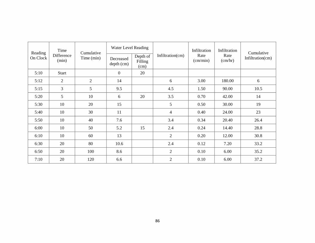
86

Reading

On Clock

Time

Difference (min)

Cumulative

Time (min)

Water Level Reading

Infiltration(cm)

Infiltration

Rate (cm/min)

Infiltration

Rate (cm/hr)

Cumulative


depth (cm)

Depth of

Filling (cm)

5:10 Start 0 20

5:12 2 2 14 6 3.00 180.00 6

5:15 3 5 9.5 4.5 1.50 90.00 10.5

5:20 5 10 6 20 3.5 0.70 42.00 14

5:30 10 20 15 5 0.50 30.00 19

5:40 10 30 11 4 0.40 24.00 23

5:50 10 40 7.6 3.4 0.34 20.40 26.4

6:00 10 50 5.2 15 2.4 0.24 14.40 28.8

6:10 10 60 13 2 0.20 12.00 30.8

6:30 20 80 10.6 2.4 0.12 7.20 33.2

6:50 20 100 8.6 2 0.10 6.00 35.2

7:10 20 120 6.6 2 0.10 6.00 37.2

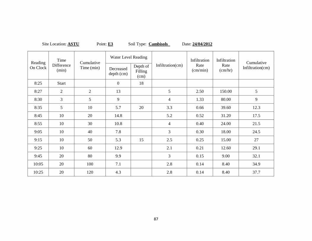
87


Reading

On Clock

Time

Difference (min)

Cumulative

Time (min)

Water Level Reading

Infiltration(cm)

Infiltration

Rate (cm/min)

Infiltration

Rate (cm/hr)

Cumulative


Depth of

Filling

(cm)

8:25 Start 0 18

8:27 2 2 13 5 2.50 150.00 5

8:30 3 5 9 4 1.33 80.00 9

8:35 5 10 5.7 20 3.3 0.66 39.60 12.3

8:45 10 20 14.8 5.2 0.52 31.20 17.5

8:55 10 30 10.8 4 0.40 24.00 21.5

9:05 10 40 7.8 3 0.30 18.00 24.5

9:15 10 50 5.3 15 2.5 0.25 15.00 27

9:25 10 60 12.9 2.1 0.21 12.60 29.1

9:45 20 80 9.9 3 0.15 9.00 32.1

10:05 20 100 7.1 2.8 0.14 8.40 34.9

10:25 20 120 4.3 2.8 0.14 8.40 37.7

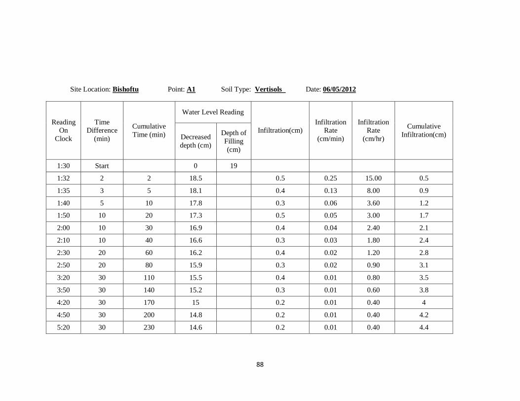
88

Site Location: Bishoftu Point: A1 Soil Type: Vertisols Date: 06/05/2012

Reading On

Clock

Time Difference

(min)

Cumulative

Time (min)

Water Level Reading


Rate

(cm/min)

Infiltration Rate

(cm/hr)

Cumulative


depth (cm)

Depth of

Filling

(cm)

1:30 Start 0 19

1:32 2 2 18.5 0.5 0.25 15.00 0.5

1:35 3 5 18.1 0.4 0.13 8.00 0.9

1:40 5 10 17.8 0.3 0.06 3.60 1.2

1:50 10 20 17.3 0.5 0.05 3.00 1.7

2:00 10 30 16.9 0.4 0.04 2.40 2.1

2:10 10 40 16.6 0.3 0.03 1.80 2.4

2:30 20 60 16.2 0.4 0.02 1.20 2.8

2:50 20 80 15.9 0.3 0.02 0.90 3.1

3:20 30 110 15.5 0.4 0.01 0.80 3.5

3:50 30 140 15.2 0.3 0.01 0.60 3.8

4:20 30 170 15 0.2 0.01 0.40 4

4:50 30 200 14.8 0.2 0.01 0.40 4.2

5:20 30 230 14.6 0.2 0.01 0.40 4.4

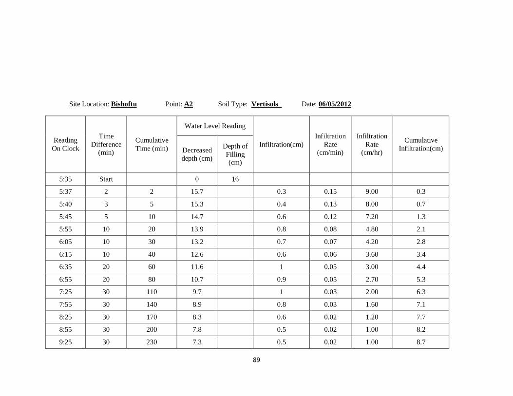
89


Reading

On Clock

Time

Difference (min)

Cumulative

Time (min)

Water Level Reading

Infiltration(cm)

Infiltration

Rate (cm/min)

Infiltration

Rate (cm/hr)

Cumulative


depth (cm)

Depth of

Filling (cm)

5:35 Start 0 16

5:37 2 2 15.7 0.3 0.15 9.00 0.3

5:40 3 5 15.3 0.4 0.13 8.00 0.7

5:45 5 10 14.7 0.6 0.12 7.20 1.3

5:55 10 20 13.9 0.8 0.08 4.80 2.1

6:05 10 30 13.2 0.7 0.07 4.20 2.8

6:15 10 40 12.6 0.6 0.06 3.60 3.4

6:35 20 60 11.6 1 0.05 3.00 4.4

6:55 20 80 10.7 0.9 0.05 2.70 5.3

7:25 30 110 9.7 1 0.03 2.00 6.3

7:55 30 140 8.9 0.8 0.03 1.60 7.1

8:25 30 170 8.3 0.6 0.02 1.20 7.7

8:55 30 200 7.8 0.5 0.02 1.00 8.2

9:25 30 230 7.3 0.5 0.02 1.00 8.7

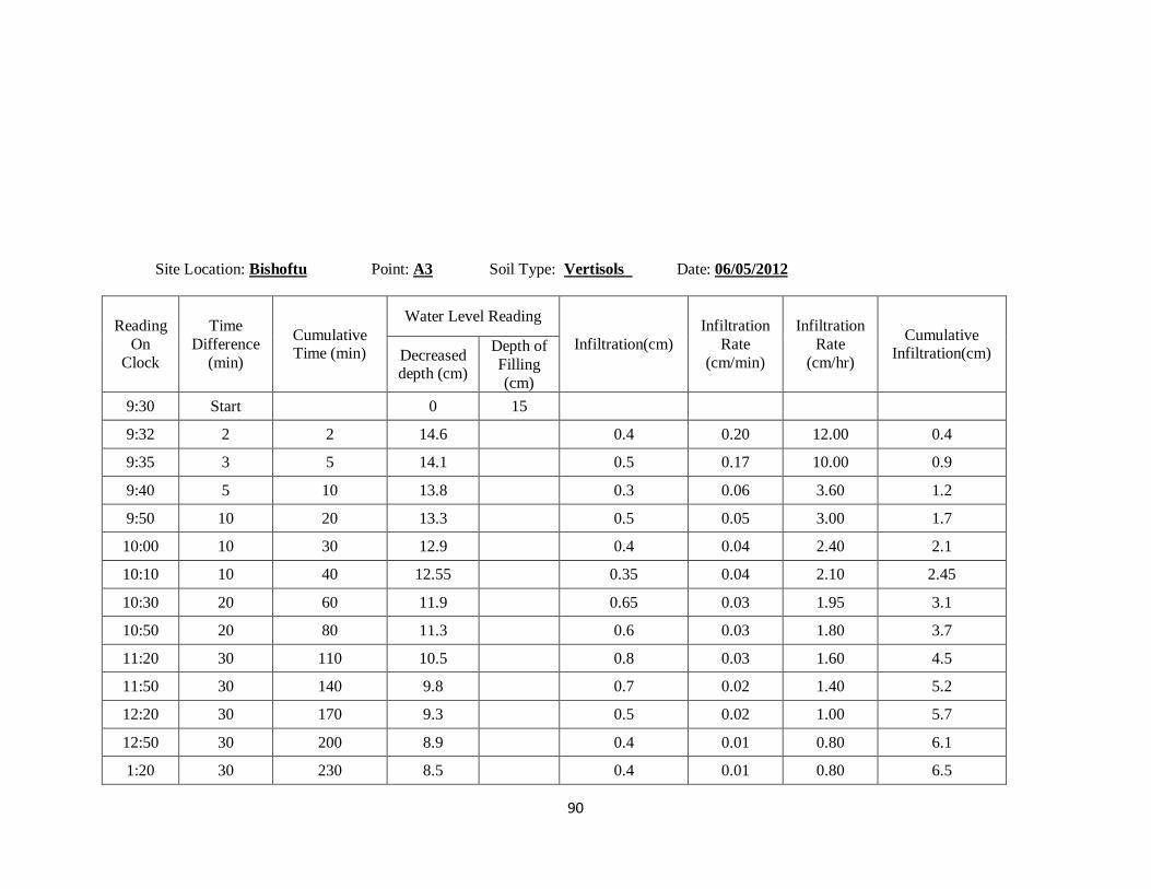
90


Reading

On

Clock

Time

Difference

(min)


Water Level Reading

Infiltration(cm)

Infiltration

Rate

(cm/min)

Infiltration

Rate

(cm/hr)


depth (cm)

Depth of

Filling

(cm)

9:30 Start 0 15

9:32 2 2 14.6 0.4 0.20 12.00 0.4

9:35 3 5 14.1 0.5 0.17 10.00 0.9

9:40 5 10 13.8 0.3 0.06 3.60 1.2

9:50 10 20 13.3 0.5 0.05 3.00 1.7

10:00 10 30 12.9 0.4 0.04 2.40 2.1

10:10 10 40 12.55 0.35 0.04 2.10 2.45

10:30 20 60 11.9 0.65 0.03 1.95 3.1

10:50 20 80 11.3 0.6 0.03 1.80 3.7

11:20 30 110 10.5 0.8 0.03 1.60 4.5

11:50 30 140 9.8 0.7 0.02 1.40 5.2

12:20 30 170 9.3 0.5 0.02 1.00 5.7

12:50 30 200 8.9 0.4 0.01 0.80 6.1

1:20 30 230 8.5 0.4 0.01 0.80 6.5

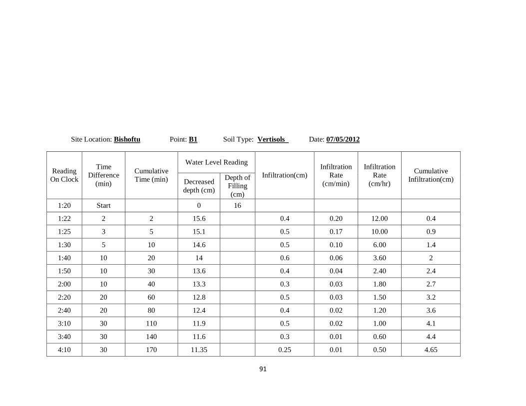
91

Site Location: Bishoftu Point: B1 Soil Type: Vertisols Date: 07/05/2012

Reading On Clock

Time

Difference

(min)


Water Level Reading

Infiltration(cm)

Infiltration

Rate

(cm/min)

Infiltration

Rate

(cm/hr)


depth (cm)

Depth of Filling

(cm)

1:20 Start 0 16

1:22 2 2 15.6 0.4 0.20 12.00 0.4

1:25 3 5 15.1 0.5 0.17 10.00 0.9

1:30 5 10 14.6 0.5 0.10 6.00 1.4

1:40 10 20 14 0.6 0.06 3.60 2

1:50 10 30 13.6 0.4 0.04 2.40 2.4

2:00 10 40 13.3 0.3 0.03 1.80 2.7

2:20 20 60 12.8 0.5 0.03 1.50 3.2

2:40 20 80 12.4 0.4 0.02 1.20 3.6

3:10 30 110 11.9 0.5 0.02 1.00 4.1

3:40 30 140 11.6 0.3 0.01 0.60 4.4

4:10 30 170 11.35 0.25 0.01 0.50 4.65

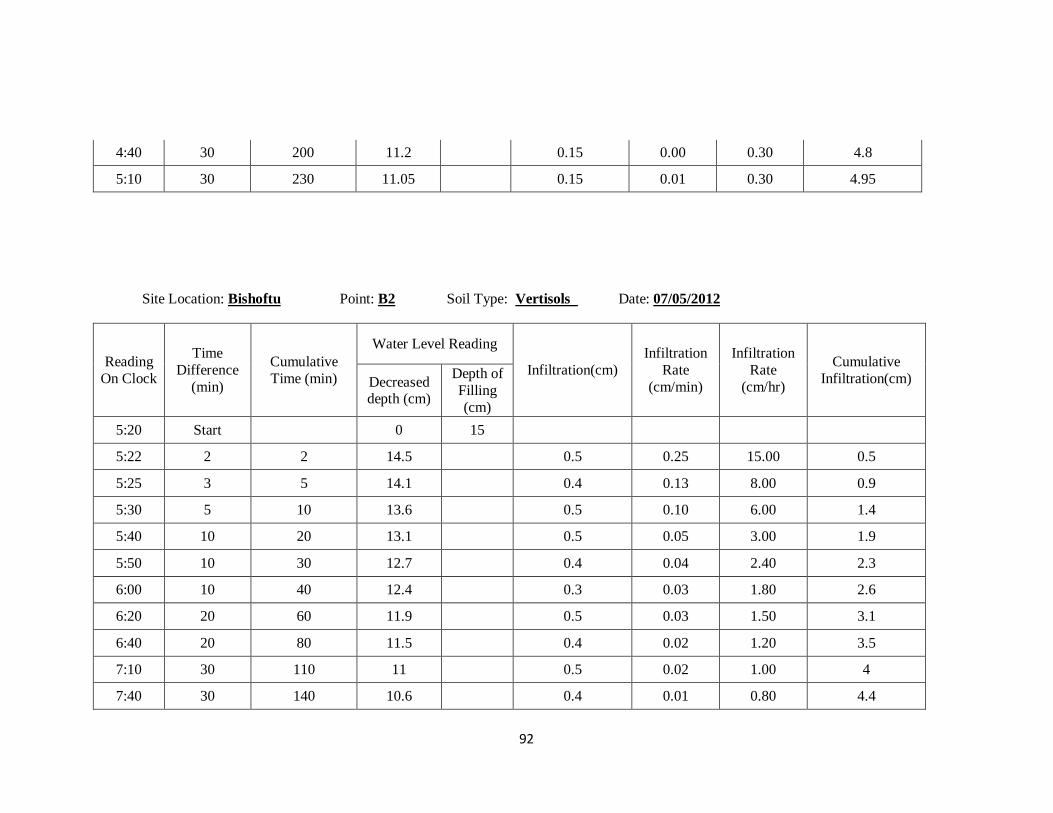
92

4:40 30 200 11.2 0.15 0.00 0.30 4.8

5:10 30 230 11.05 0.15 0.01 0.30 4.95


Reading

On Clock

Time

Difference

(min)

Cumulative

Time (min)

Water Level Reading

Infiltration(cm)

Infiltration

Rate

(cm/min)

Infiltration

Rate

(cm/hr)

Cumulative


Depth of

Filling

(cm)

5:20 Start 0 15

5:22 2 2 14.5 0.5 0.25 15.00 0.5

5:25 3 5 14.1 0.4 0.13 8.00 0.9

5:30 5 10 13.6 0.5 0.10 6.00 1.4

5:40 10 20 13.1 0.5 0.05 3.00 1.9

5:50 10 30 12.7 0.4 0.04 2.40 2.3

6:00 10 40 12.4 0.3 0.03 1.80 2.6

6:20 20 60 11.9 0.5 0.03 1.50 3.1

6:40 20 80 11.5 0.4 0.02 1.20 3.5

7:10 30 110 11 0.5 0.02 1.00 4

7:40 30 140 10.6 0.4 0.01 0.80 4.4

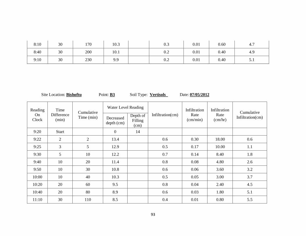
93

8:10 30 170 10.3 0.3 0.01 0.60 4.7

8:40 30 200 10.1 0.2 0.01 0.40 4.9

9:10 30 230 9.9 0.2 0.01 0.40 5.1


Reading On

Clock

Time Difference

(min)

Cumulative

Time (min)

Water Level Reading


Rate

(cm/min)

Infiltration Rate

(cm/hr)

Cumulative


Depth of

Filling

(cm)

9:20 Start 0 14

9:22 2 2 13.4 0.6 0.30 18.00 0.6

9:25 3 5 12.9 0.5 0.17 10.00 1.1

9:30 5 10 12.2 0.7 0.14 8.40 1.8

9:40 10 20 11.4 0.8 0.08 4.80 2.6

9:50 10 30 10.8 0.6 0.06 3.60 3.2

10:00 10 40 10.3 0.5 0.05 3.00 3.7

10:20 20 60 9.5 0.8 0.04 2.40 4.5

10:40 20 80 8.9 0.6 0.03 1.80 5.1

11:10 30 110 8.5 0.4 0.01 0.80 5.5

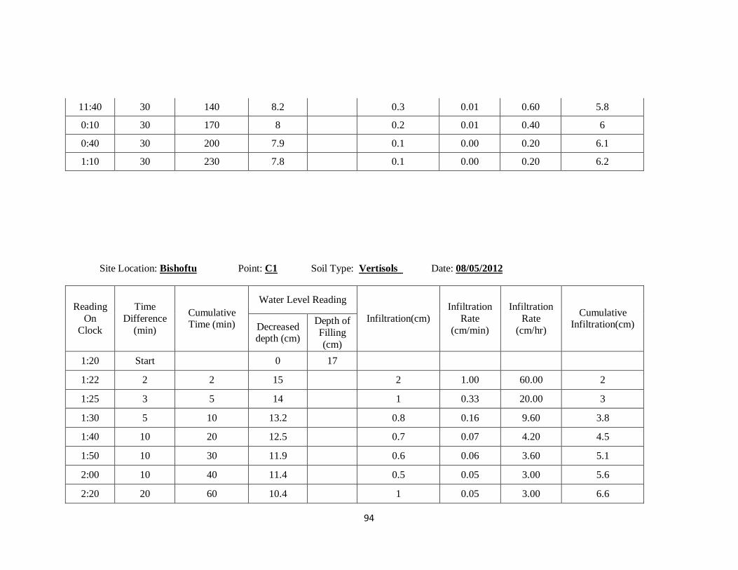
94

11:40 30 140 8.2 0.3 0.01 0.60 5.8

0:10 30 170 8 0.2 0.01 0.40 6

0:40 30 200 7.9 0.1 0.00 0.20 6.1

1:10 30 230 7.8 0.1 0.00 0.20 6.2

Site Location: Bishoftu Point: C1 Soil Type: Vertisols Date: 08/05/2012

Reading

On

Clock

Time

Difference

(min)


Water Level Reading

Infiltration(cm)

Infiltration

Rate

(cm/min)

Infiltration

Rate

(cm/hr)


depth (cm)

Depth of

Filling

(cm)

1:20 Start 0 17

1:22 2 2 15 2 1.00 60.00 2

1:25 3 5 14 1 0.33 20.00 3

1:30 5 10 13.2 0.8 0.16 9.60 3.8

1:40 10 20 12.5 0.7 0.07 4.20 4.5

1:50 10 30 11.9 0.6 0.06 3.60 5.1

2:00 10 40 11.4 0.5 0.05 3.00 5.6

2:20 20 60 10.4 1 0.05 3.00 6.6

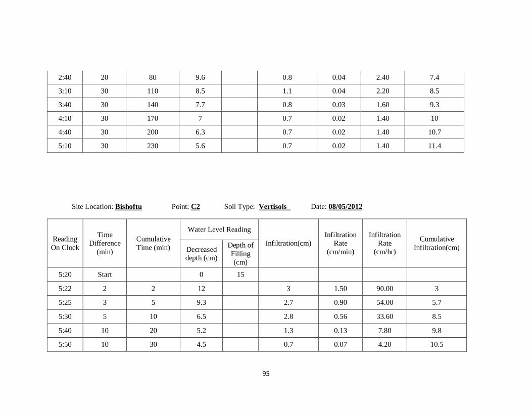
95

2:40 20 80 9.6 0.8 0.04 2.40 7.4

3:10 30 110 8.5 1.1 0.04 2.20 8.5

3:40 30 140 7.7 0.8 0.03 1.60 9.3

4:10 30 170 7 0.7 0.02 1.40 10

4:40 30 200 6.3 0.7 0.02 1.40 10.7

5:10 30 230 5.6 0.7 0.02 1.40 11.4


Reading

On Clock

Time Difference

(min)

Cumulative

Time (min)

Water Level Reading


Rate

(cm/min)

Infiltration Rate

(cm/hr)

Cumulative


Depth of

Filling

(cm)

5:20 Start 0 15

5:22 2 2 12 3 1.50 90.00 3

5:25 3 5 9.3 2.7 0.90 54.00 5.7

5:30 5 10 6.5 2.8 0.56 33.60 8.5

5:40 10 20 5.2 1.3 0.13 7.80 9.8

5:50 10 30 4.5 0.7 0.07 4.20 10.5

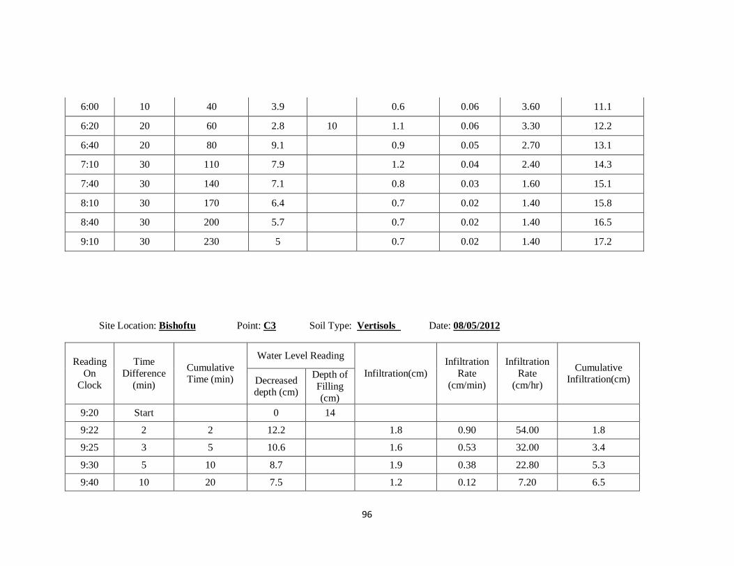
96

6:00 10 40 3.9 0.6 0.06 3.60 11.1

6:20 20 60 2.8 10 1.1 0.06 3.30 12.2

6:40 20 80 9.1 0.9 0.05 2.70 13.1

7:10 30 110 7.9 1.2 0.04 2.40 14.3

7:40 30 140 7.1 0.8 0.03 1.60 15.1

8:10 30 170 6.4 0.7 0.02 1.40 15.8

8:40 30 200 5.7 0.7 0.02 1.40 16.5

9:10 30 230 5 0.7 0.02 1.40 17.2


Reading

On

Clock

Time

Difference

(min)


Water Level Reading

Infiltration(cm)

Infiltration

Rate

(cm/min)

Infiltration

Rate

(cm/hr)


depth (cm)

Depth of

Filling

(cm)

9:20 Start 0 14

9:22 2 2 12.2 1.8 0.90 54.00 1.8

9:25 3 5 10.6 1.6 0.53 32.00 3.4

9:30 5 10 8.7 1.9 0.38 22.80 5.3

9:40 10 20 7.5 1.2 0.12 7.20 6.5

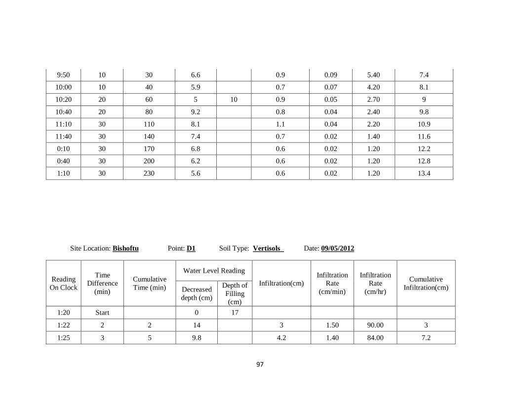
97

9:50 10 30 6.6 0.9 0.09 5.40 7.4

10:00 10 40 5.9 0.7 0.07 4.20 8.1

10:20 20 60 5 10 0.9 0.05 2.70 9

10:40 20 80 9.2 0.8 0.04 2.40 9.8

11:10 30 110 8.1 1.1 0.04 2.20 10.9

11:40 30 140 7.4 0.7 0.02 1.40 11.6

0:10 30 170 6.8 0.6 0.02 1.20 12.2

0:40 30 200 6.2 0.6 0.02 1.20 12.8

1:10 30 230 5.6 0.6 0.02 1.20 13.4

Site Location: Bishoftu Point: D1 Soil Type: Vertisols Date: 09/05/2012

Reading

On Clock

Time Difference

(min)

Cumulative

Time (min)

Water Level Reading


Rate

(cm/min)

Infiltration Rate

(cm/hr)

Cumulative


depth (cm)

Depth of

Filling (cm)

1:20 Start 0 17

1:22 2 2 14 3 1.50 90.00 3

1:25 3 5 9.8 4.2 1.40 84.00 7.2

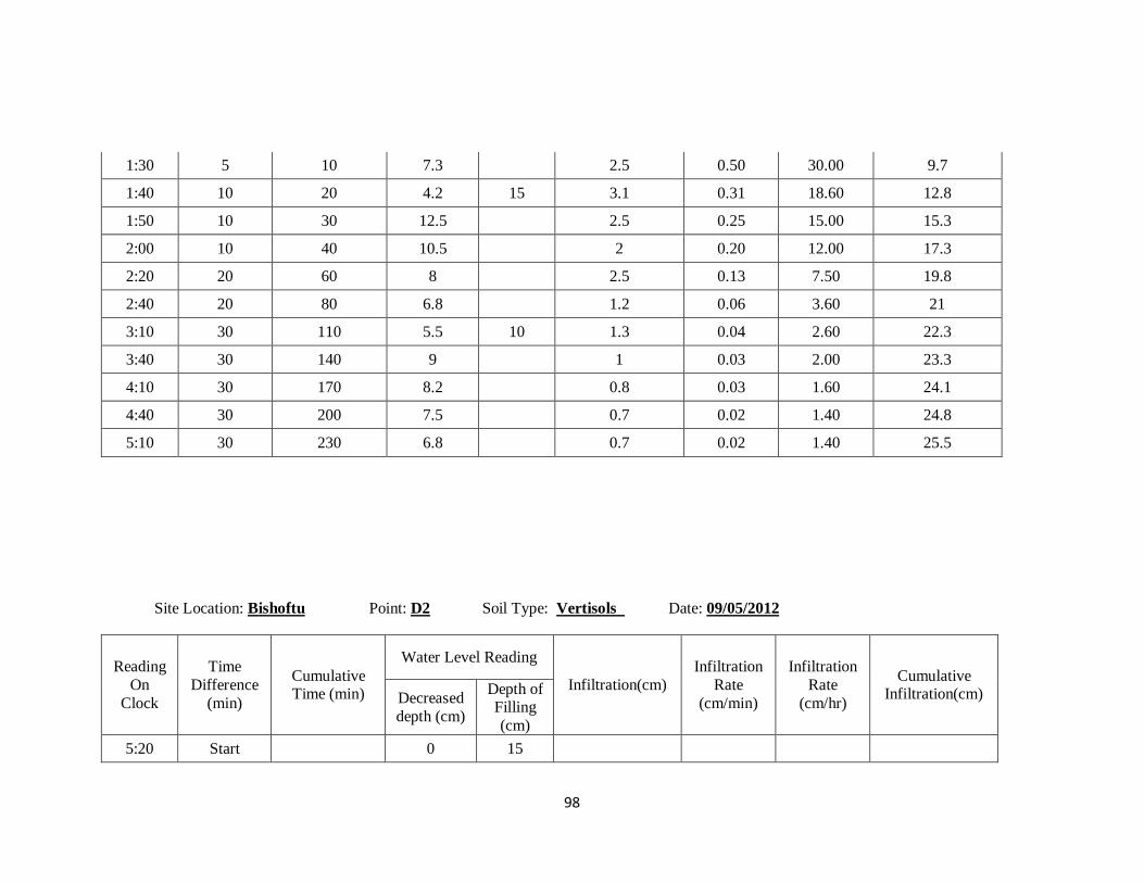
98

1:30 5 10 7.3 2.5 0.50 30.00 9.7

1:40 10 20 4.2 15 3.1 0.31 18.60 12.8

1:50 10 30 12.5 2.5 0.25 15.00 15.3

2:00 10 40 10.5 2 0.20 12.00 17.3

2:20 20 60 8 2.5 0.13 7.50 19.8

2:40 20 80 6.8 1.2 0.06 3.60 21

3:10 30 110 5.5 10 1.3 0.04 2.60 22.3

3:40 30 140 9 1 0.03 2.00 23.3

4:10 30 170 8.2 0.8 0.03 1.60 24.1

4:40 30 200 7.5 0.7 0.02 1.40 24.8

5:10 30 230 6.8 0.7 0.02 1.40 25.5


Reading

On

Clock

Time

Difference

(min)


Water Level Reading

Infiltration(cm)

Infiltration

Rate

(cm/min)

Infiltration

Rate

(cm/hr)


depth (cm)

Depth of Filling

(cm)

5:20 Start 0 15

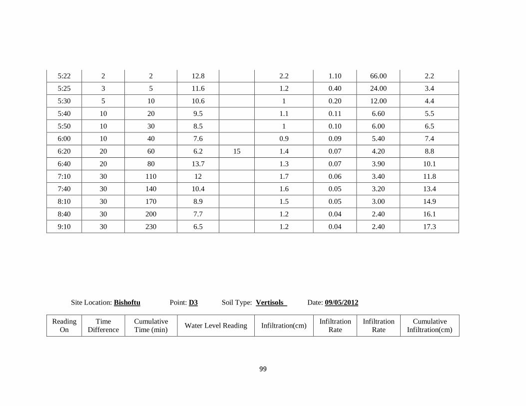
99

5:22 2 2 12.8 2.2 1.10 66.00 2.2

5:25 3 5 11.6 1.2 0.40 24.00 3.4

5:30 5 10 10.6 1 0.20 12.00 4.4

5:40 10 20 9.5 1.1 0.11 6.60 5.5

5:50 10 30 8.5 1 0.10 6.00 6.5

6:00 10 40 7.6 0.9 0.09 5.40 7.4

6:20 20 60 6.2 15 1.4 0.07 4.20 8.8

6:40 20 80 13.7 1.3 0.07 3.90 10.1

7:10 30 110 12 1.7 0.06 3.40 11.8

7:40 30 140 10.4 1.6 0.05 3.20 13.4

8:10 30 170 8.9 1.5 0.05 3.00 14.9

8:40 30 200 7.7 1.2 0.04 2.40 16.1

9:10 30 230 6.5 1.2 0.04 2.40 17.3


Reading On

Time Difference


Water Level Reading Infiltration(cm) Infiltration

Rate Infiltration

Rate Cumulative

Infiltration(cm)

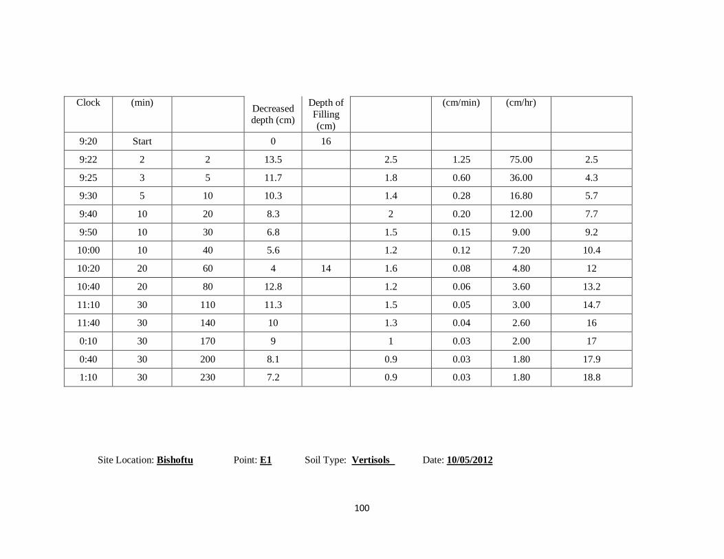
100

Clock (min) Decreased depth (cm)

Depth of

Filling

(cm)

(cm/min) (cm/hr)

9:20 Start 0 16

9:22 2 2 13.5 2.5 1.25 75.00 2.5

9:25 3 5 11.7 1.8 0.60 36.00 4.3

9:30 5 10 10.3 1.4 0.28 16.80 5.7

9:40 10 20 8.3 2 0.20 12.00 7.7

9:50 10 30 6.8 1.5 0.15 9.00 9.2

10:00 10 40 5.6 1.2 0.12 7.20 10.4

10:20 20 60 4 14 1.6 0.08 4.80 12

10:40 20 80 12.8 1.2 0.06 3.60 13.2

11:10 30 110 11.3 1.5 0.05 3.00 14.7

11:40 30 140 10 1.3 0.04 2.60 16

0:10 30 170 9 1 0.03 2.00 17

0:40 30 200 8.1 0.9 0.03 1.80 17.9

1:10 30 230 7.2 0.9 0.03 1.80 18.8

Site Location: Bishoftu Point: E1 Soil Type: Vertisols Date: 10/05/2012

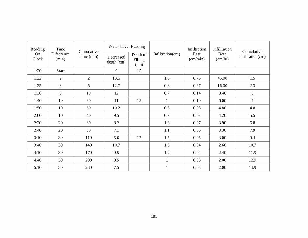
101

Reading On

Clock

Time Difference

(min)

Cumulative

Time (min)

Water Level Reading


Rate

(cm/min)

Infiltration Rate

(cm/hr)

Cumulative


depth (cm)

Depth of

Filling (cm)

1:20 Start 0 15

1:22 2 2 13.5 1.5 0.75 45.00 1.5

1:25 3 5 12.7 0.8 0.27 16.00 2.3

1:30 5 10 12 0.7 0.14 8.40 3

1:40 10 20 11 15 1 0.10 6.00 4

1:50 10 30 10.2 0.8 0.08 4.80 4.8

2:00 10 40 9.5 0.7 0.07 4.20 5.5

2:20 20 60 8.2 1.3 0.07 3.90 6.8

2:40 20 80 7.1 1.1 0.06 3.30 7.9

3:10 30 110 5.6 12 1.5 0.05 3.00 9.4

3:40 30 140 10.7 1.3 0.04 2.60 10.7

4:10 30 170 9.5 1.2 0.04 2.40 11.9

4:40 30 200 8.5 1 0.03 2.00 12.9

5:10 30 230 7.5 1 0.03 2.00 13.9

MODELING INFILTRATION CAPACITY OF MAJOR SOILS

Documents